g-Jitter effects on spherical diffusion flames

William E. Mell, Kevin B. McGrattan, Howard R. Baum: g-Jitter Effects on Spherical Diffusion Flames

William E. Mell, Kevin B. McGrattan, Howard R. Baum

g-Jitter Effects on Spherical Diffusion Flames

Acceleration disturbances or g-jitter exist in all reduced gravi-ty experimental platforms. These disturbances often have a fullythree-dimensional orientation and are transient. An importantelement in experimental design, therefore, is a determination ofhow sensitive the physical processes under investigation may beto the expected g-jitter. Very few experimental studies exist thatare focused on quantifying acceptable levels of g-jitter due totheir expense and the wide range of relevant parameters. Athree-dimensional fully transient computer simulation approachwas developed, validated, and used to assess the potential thata given acceleration disturbance will have an unacceptableinfluence on spherical diffusion flames. An emphasis was put oncomputational efficiency resulting in the use of a simple, mixturefraction based, combustion model. Given the limitations of thismodel the simulation provided accurate predictions of flamebehaviour in experiments conducted in NASAs drop tower andaircraft reduced gravity platforms. Spherical diffusion flames inacceleration environments characteristic of the InternationalSpace Station were also simulated. The results implied that apassive isolation system combined with appropriate schedulingof crew activity would provide a sufficiently disturbance freeenvironment for spherical diffusion flame experiments.

Mail address:

William MellBuilding and Fire Research Laboratory, National Institute of Standards andTechnology, 100 Bureau Drive, Stop 8663, Gaithersburg, MD [email protected], (201)975-4797; (301)975-4052 (fax)

Paper submitted: 23.09.03Submission of final revised version: 14.09.04Paper accepted: 13.10.04

12 © Z-Tec Publishing, Bremen Microgravity sci. technol. XV/4 (2004)

1. Introduction and Background

By conducting experiments in reduced gravity, scientists canoften isolate and study physical phenomena in ways not possi-ble on Earth. In the area of combustion, buoyancy generatedflow (often turbulent) influences the dynamics and structure ofa flame in a complex manner. As a result the combustionprocess is more difficult to control and the productive place-ment of diagnostic probes more problematic.

Ideally, in sufficiently reduced gravity, experiments can beconducted free from the confounding influences of buoyancy.An important question is, therefore, what is the character of asufficiently small acceleration disturbance? This issue is rele-vant to experiments in the areas of biotechnology, combustion,fluid physics, fundamental physics, and material science. Ineach of these areas guidelines regarding acceptable accelerationlimits have been proposed [1]. These guidelines were oftendeveloped based on experiments which suffered from theeffects of unexpected and undesired acceleration disturbancesor g-jitter (e.g., Struk et al. [2]). Because of the expense ofreduced gravity experiments there has been little effort to con-duct experiments solely for the purpose of assessing the effectsof acceleration disturbances on the combustion process. Anexception to this in the area of combustion is the work byFeikema [3] in which the effects of acceleration disturbances,present on the KC-135 aircraft, on spherical diffusion flameswas investigated. Theoretical investigations on the relevance ofg-jitter on natural convection and diffusion processes in thepresence of thermal gradients has been conducted by Ostrach[4, 5] and Kamotani et al.[6].

Using numerical simulations, Kaplan et al. [7] and Long etal. [8] considered g-jitter effects on axially-symmetric jets.Kaplan et al. [7] simulated a laminar ethylene/air noncoflowingjet diffusion flame to better understand the dynamics andbehavior of heavily sooting flames in a variety of gravity envi-

Microgravity sci. technol. XV/4 (2004) 13

ronments. The influence of g-jitter was investigated by applyinga sinusoidal acceleration in the axial direction of amplitude0.01ge and frequency 1 Hz. The flame height was found to oscil-late with the 1 Hz frequency. Long et al. [8] simulated a coflow-ing methane/air jet with g varying between ±0.01ge axial direc-tion. The flame structure was found to be insensitive to theselevels of acceleration. The differing results of these two studies,in regard to the influence of g-jitter, imply that the relevance ofg-jitter is problem dependent and should be assessed for eachcombustion system.

While the simulation approach can be applied to a variety ofcombustion problems the focus here will be on spherical diffu-sion flames. Results from spherical diffusion flame experimentsconducted in aircraft [3] and drop tower [9, 10] reduced gravityfacilities are available. Experiments on the International SpaceStation (ISS) are also planned. Because of the spherical sym-metry of these flames (in the absence of sufficiently large accel-eration disturbances) one-dimensional numerical simulationshave been used in theoretical investigations [9, 10]. Whenacceleration disturbances break the spherical symmetry a multi-dimensional numerical simulation is needed. Thus, because oftheir relatively simple geometry, the availability of experimen-tal results in a range of reduced gravity facilities, and their con-tinued use in experimental and numerical studies spherical dif-fusion flames are good first step in code validation and applica-tion. Combustion scenarios that involve more complex geome-try will be considered at a later date.

Acceleration disturbances exist in all the commonly usedreduced gravity facilities: drop towers, aircraft, sounding rock-ets, space shuttle, and the ISS. The quality and duration of thereduced gravity varies across these facilities. Ideally, the dura-tion and magnitude of reduced gravity is: drop towers (2 - 10s,10-5ge), aircraft (7 - 20 s, 10-3ge - 10-4ge), sounding rockets (min-utes, 10-5ge)> space shuttle (≈17 days, 10-5ge, with proper isola-tion from disturbance), ISS (up to years; 10-6ge with proper iso-lation from disturbance). This ordering is based on the durationeach facility operates in reduced gravity. The actual duration ofacceptable reduced gravity may be less and depends on theexperiment in question and environmental conditions. Forexample, routine and essential activities on the the space shuttleand ISS introduce acceleration disturbances (e.g., crew exer-cise, docking of the space shuttle to the ISS). Because of this,hardware systems have been developed to isolate an experi-mental rack from acceleration disturbances on the ISS.Depending on its level of sophistication the development,installation, maintenance, and operation of these systems can beexpensive in both a financial and crew commitment sense. Also,given the lack of a systematic study of g-jitter effects on a givenexperiment, it is often not certain what degree of isolation (orlimit on the acceleration disturbance) is required. A suitablyaccurate computer simulation tool could be used to easily andrelatively cheaply predict the potential that a given accelerationdisturbance would corrupt a planned experiment.

Thoroughly quantifying the impact of a given g-jitter distur-bance on a flame was not the aim of this work. That wouldrequire experimental data at a level of detail that does notpresently exist, especially at smaller magnitudes of accelerationdisturbances. Instead, the objective was to develop a reasonablyfast (computationally efficient) numerical model and then deter-mine if it provided qualitatively accurate but useful predictionsof the effect of three-dimensional time varying acceleration dis-turbances on a spherical diffusion flame. To do this a measureof the effect of g-jitter was required. For large enough accelera-tion disturbances the spherical flame will visually break sym-metry. For this reason in most experimental studies visualobservation of flame shape has been used as a measure of g-jit-ter affects [2, 3]. However, for smaller disturbances the flamemay be adversely affected but not in a visually obvious or aseasily measurable way. In this study the measure used for g-jit-ter effects (for small acceleration disturbances) is the differencein the temperature field between a simulation with a givenacceleration disturbance and one with no disturbance. Thismeasure was somewhat arbitrary but since an acceleration dis-turbance most directly affects a flame through buoyancy it is areasonable initial choice. The temperature field will also bepresent in any combustion model, unlike soot, products of sec-ondary reactions, etc. which depend on the type of combustionmodel and/or fuel used. The influence of acceleration distur-bance on specific combustion products, such as soot production,is outside the scope of the present paper.

In the following sections the model equations and anoverview of the numerical approach to solve them are present-ed. The simulation approach is then validated against a numberof experimental studies both without and with acceleration dis-turbances. Next the simulation approach is applied to test thevalidity of the integrated transient acceleration limit for a spher-ical diffusion flame. Finally, measured and predicted levels ofacceleration disturbances in the ISS are used in spherical diffu-sion flame simulations to investigate the need for a system toisolate combustion experiments from g-jitter.

2. Modeling Approach

2.1. Conservation EquationsThe governing equations for low Mach number flow with com-bustion were derived following Rehm and Baum [11] andMcGrattan et al. [12]. Ideal gases and Fickian diffusion wereassumed. The equation for conservation of total mass is

The equation for conservation of momentum is


.u utρ ρ ρ∂ + ⋅∇ = −∇ ⋅

∂(1)

( )1 ,u H u w gt

ρ ρ τρ ∞

∂ + ∇ − × = − + ∇ ⋅ ∂

(2)

2 21 1 1 1 ,2 2d du uρ ρ

ρ ρ∞

∇ ≡ ∇ + ∇ ≅ ∇ + ∇ (3)H

The vector identity (u · ∇) u = (l/2)∇|u|2 - u x ω has been used.The assumption made in Eq. (3) implies that (1/ρ — l/ρ∞)∇ρd isnegligible. Physically this amounts to assuming that the baro-clinic torque has a negligible contribution to vorticity genera-tion (relative to buoyancy). With this assumption a constantcoefficient PDE for the pressure can be formed by taking thedivergence of the momentum equation [Eq.(2)], see Sec. 4. Thispressure PDE was solved in a computationally efficient andaccurate manner using a direct solver. The baroclinic torque wasthen restored using the pressure from the previous time step[12]. The equation for the conservation of species is

Here the diffusion coefficient for species i into the gas mixture,Di,mix, was approximated by Di,mix ≈ DN2

the diffusion coefficientof species i into nitrogen. The equation of state is

The equation for conservation of energy in terms of the mixtureenthalpy, h, is

note that the energy release associated with chemical reactionsis not explicitly present but was accounted for by h [13], seeEq.(10). Here

are the enthalpy of the mixture and of species i, respectively.The temperature only dependence of the enthalpy of ideal gaseswas used. Note, cp =Σi Yi dhi/dT is the mixture specific heat. Thespectral radiation transport equation (RTE) for thermal radiationin an absorbing-emitting, non-scattering gas is:

This equation was solved numerically using the finite volumeapproach [14]. The details of the implementation of thisapproach are in [12]. The spectral dependence was approximat-ed by dividing the spectrum into a number of bands and solvingEq. (9) for each band. Absorption coefficients were determined

using a narrow-band model RadCal [15] and tabulated as afunction of the mixture fraction (see Sec. 3.3). The solution ofEq. (9) using 6 spectral bands required approximately 50% ofthe total cpu time. The molar heat of combustion for a givenchemical reaction is, for constant pressure,

The simplified stoichiometric relation of a chemical reactionwith a hydrocarbon fuel

CxHy + a (O2 + 3.76 N2) →xCO2 + (y/2) H2O + 3.76 a N2 (11)

(a = x + y/4; a, x, y ≥ 0) was assumed. The mass consumptionrate term for any species (except N2 which is chemically inac-tive) can be written in terms of one single specific species. Interms of the fuel mass consumption rate (note νreactant < 0; νproduct

> 0):

With this expression the heat release rate of the combustionprocess can be expressed in terms of the heat of combustion:

Here ∆hc = ∆h_

c / MF is the mass based heat of combustion andthe fact that νF = -1 has been used.

2.2 Divergence constraintA general divergence constraint on the velocity can be derivedby taking the material (or Lagrangian) derivative of the equationof state

and using Eqs. (1), (5), DT/Dt from Dh/Dt (eq. (7) where h isexpressed in Eq. (8):

Microgravity sci. technol. XV/4 (2004)14


2( ) ( ) .3

Tu u uτ µ ≡ ∇ + ∇ − ∇ ⋅ Ι (4)

''',( ) ( ) .i

i i i mix i iY u Y Y u D Y mt

∂ + ⋅∇ = − ∇ ⋅ + ∇ ⋅ ∇ +∂ρ ρ ρ ρ (5)

,ˆ ˆ ˆ( , ) ( )[ ( ) ( , )].bs I x s k x I x I x sλ λ λ λ⋅∇ = − (9)

0,( , ) ( , ) ( ), ( ) ( ') '

o

T

i i i i p iTi

h x t Y x t h T h T h c T dT= = +∑ ∫ (8)

( )

'',

oi i mix i R

i

h u h Tt

dph D Y qdt

∂ + ⋅∇ = ∇ ⋅ ∇ +∂ ∇ ⋅ − ∇ ⋅ + ∑

ρ ρ λ

ρ(7)

0 ( ) / / .i ii

p t R T Y M R T M= =∑ρ ρ (6)

( ) ( )

( )

'',

''',

1 1

1 1

po

p o

i mix i i Ri

ii mix i i

i ii i p

c Tu p t T

c T p

D Y h q

hM MD Y mM M c T

∇ ⋅ = − + ∇ ⋅ ∇ +

∇ ⋅∇ −∇ ⋅

+ ∇ ⋅ ∇ + − ⋅

∑

∑ ∑

ρλ

ρ

ρ

ρρ ρ

(15)

( ) ( ) .c i i i i ii i

h v h T v h T M∆ = − = −∑ ∑ (10)

2

2 2

''' ''' ( ), , 1,

( ), , / 2,H

ii i F i F o

F

co

vMm r m r v v

vMa v x v O y

= = = −

= − = =(12)

''' '''''' ''' ''' .

( ) ( )F F

i i i i i i c F ci iF F

m mQ h m v h M h m hvM vM

= − = − = − ∆ = − ∆∑ ∑(13)

10 i

i i

DYRT D R DTp R TM Dt M Dt M Dt

ρ ρ ρ= + + ∑ (14)


A similar expression for the divergence constraint has been usedin simulations by Bell et al. [16] of vortex flame interaction forthe case of an open domain (p·o = 0) and neglecting thermal radi-ation. Note that if the physical domain being simulated isenclosed then p·o (t) ≠ 0. In this case p·o (t) is determined using theequation derived from integrating the divergence constraintover the entire domain. Equation (15) can be simplified usingthe assumption that the ratio of specific heats γ for each speciesis equal to the value for diatomic gases, γi = 7/5. The basis forthis assumption is that nitrogen is the dominant species.

where the implication that the molar specific heats are constantfollows from c

_p,i - c

_v,i= R. With this assumption the divergence

constraint can be written

where the relation

has been used to combine the two diffusion terms in Eq. (15).Note that while the mass based specific heats, cp,i, have beenassumed to be independent of temperature they are dependenton the molecular weight of the species. It is especially impor-tant to include this dependence when the fuel and oxidantspecies have significantly different molecular weights, as theydo in the cases considered below (hydrogen based fuel in air).In each form of the divergence constraint the mass consumptionterms are, using Eqs. (12) and (13)

2.3 Mixture fraction based combustion modelModels of detailed chemical kinetics are too computationallyexpensive to implement in multidimensional simulations forengineering applications. Also, for the present purpose of thesimulation code - to simulate g-jitter effects - such sophisticat-ed models are not required. Instead, combustion models that are

less computationally expensive but proven in terms of predict-ing temperatures are suitable for a first step to simulating three-dimensional transient g-jitter effects. One such approach, thefast reaction or flame sheet model, is based on the assumptionthat when fuel and oxygen mix they immediately (over the mix-ing time scale) react to completion. Further development of theapproach would possibly include simple one-step finite ratereactions with Arrhenius kinetics. The major disadvantages ofthe flame sheet model are that the reaction rate is not tempera-ture dependent and the formation of products due to secondary,slower, reactions are not well predicted. Applying the flamesheet assumption, YFYO2

= 0 to the following definition of a mix-ture fraction, Z,

the dependence of YF and YO2on Z can be easily determined.

Here YF∞ is the fuel mass fraction in the fuel stream; Y ∞

02 is theoxygen mass fraction in the fresh oxidant; and rO2

was definedin Eq. (12). The conservation equation for Z is obtained fromcombining the conservation equations for YF and YO2

accordingto Eq. (20) and using Eq. (12) and the assumption that Di, mix =D (see Eq. (29)):

With this equation, Eq. (12), and zero boundary conditions (at Z= 0,1) the dependence of YCO2

and Yh2o on Z can be determined.The divergence constraint, Eq. (17), in the context of the flamesheet mixture fraction combustion model (∇Yi = Yi’ ∇Z, DYi / Dt= Yi’ (∇Z where Y' ≡ dYi / dZ) is

where

m·F’’’ = Y’F ∇ · (ρD∇Z) -∇ · (Y’F ρD∇Z). (23)

2.4 Transport coefficientsThe viscosity, thermal conductivity, and material diffusivity areapproximated from kinetic theory [13, 17]. The dynamic vis-cosity for species i is


, ,, ,

, ,

7,5 , constant,p i p ii p i p v i v

v i v i

c cc c c c

c cγ γ= = = = ⇒ = =

(16)

( ) ( )

( ) '', ,

'''

1 1

1 ,

po

p o

p i i mix i Ri

ii

i i p

c Tu p t T

c T p

c T D Y q

hM mM c T

ρλ

ρ

ρ

ρ

∇ ⋅ = − + ∇ ⋅ ∇ +

∇ ⋅ ∇ −∇ ⋅

+ −

∑

∑

(17)

, ,

,

constant, ,1 1p i p i p i

ii i

p i

i p

R Rc c Y cM M

cMM c

γ γγ γ

= = = =− −

⇒ =

∑(18)

''' '''1 1 .ii i ci F

i i p F F p

M vh hM m mM c T v M c Tρ ρ

∆− = −

∑∑ (19)

2 2 2

2 2

( ), 0 1,O F O O

O F O

r Y Y YZ z

r Y Y

∞

∞ ∞

− −≡ ≤ ≤

+(20)

( ) ( )Z u Z Z u D Zt

ρ ρ ρ ρ∂ + ⋅∇ = − ∇ ⋅ + ∇ ⋅ ∇∂

(21)

( ) ( )

( )' '',

'''

1 1

1 ,

po

p o

i p i Ri

ii c

FF F p

c Tu p t T

c T p

Y c T D Z q

M vh m

v M c T

∇ ⋅ = − + ∇ ⋅ ∇ −

∇ ⋅ ∇ −∇ ⋅

∆ − −

∑

∑

ρλ

ρ

ρ

ρ

(22)

7 1/ 2

2

26,69 10 ( )ii

i

M Tµ

σ

−×=

Ω(24)


where σi is the Lennard-Jones hard-sphere diameter and Ω is thecollision integral which is an empirical function of the temper-ature. The dynamic viscosity of the gaseous mixture is given by[13]:

The thermal conductivity of species i is based on the dynamicviscosity [13]:

The thermal conductivity of the gaseous mixture is [13]:

As mentioned above, the mass diffusivity of species i into thegaseous mixture is approximated by the mass diffusivity i intonitrogen, Di,mix ≈ Di,N2

. The binary mass diffusion coefficientsare [13, 17]:

where Mi,N2= 2(1/Mi + l/MN2

)-1, σi,N2= (σi + σN2

)/2, and ΩD isthe diffusion collision integral which is an empirical function of

the temperature. The mass diffusivity of the gaseous mixture is:Look-up tables of the transport coefficients, as functions of Zand T, are made before the simulation begins.

3. Numerical Approach

The equations which were solved numerically are Eq. (1), con-servation of total mass; Eq. (2), conservation of momentum; Eq.(21), conservation of mixture fraction; Eq. (22), divergenceconstraint; Eq. (6), equation of state. The pressure field, H, wasobtained by solving a constant coefficient Poisson equationobtained by taking the divergence of the momentum equation,Eq. (2), written in the form ∂u / ∂t = -∇H - F,

where F contains the convection, buoyancy, and viscous fluxterms. The temporal and spatial discretization approaches arediscussed in detail in McGrattan et al. [12]. For completeness anoverview is given here.

Explicit second order Runge-Kutta time stepping was used.

This was a two stage procedure in which first a predicted andthen a corrected value of dependent variable at next time leveltn+1 =tn + ∆t was found:

Here f is a dependent variable, f p, f c are its predicted and cor-rected values respectively, and f·n = (∂f/∂t)n was evaluated usingthe conservation equation for f. The time stepping procedureproceeded as follows. First the thermodynamic scalar variablesρp, (ρΖ)p were determined using Eq. (31) and their conservationequations, Eqs. (1), (21). In order to obtain the predicted veloc-ity field, up, the pressure field Hn was required in (∂f / ∂t)n fromEq. (2). Equation (30) was used to obtain Hn with, with the timederivative of the velocity divergence evaluated as

based on Eq. (31). The temperature, Tp, was determined fromthe equation of state, Eq. (6). At this point all predicted valuesof the variables an tn+1 were known. Next the corrected valueswere computed in a similar manner using Eq. (32).

Note that this approaches formally ensures that the diver-gence of up (or uc) equaled the divergence constraint using pre-dicted (or corrected) variables. For example, using Eq. (31) thedivergence of the predicted velocity is

Just how equal these two quantities are depends on errors inher-ent in the finite differencing and in the solution of the pressurePDE, Eq. (30). In the current approach second order spatial dif-ferencing on a rectilinear grid was used. The pressure PDE wassolved to machine accuracy through the use of a fast direct(non-iterative) solver [12]. Variables on the grid are staggeredwith cell-centered scalars and face-centered velocities and flux-es. Convective terms were written as upwind-biased differencesin the predictor step and downwind-biased differences in thecorrector step. Central differences were used for the thermal andmass diffusion terms.

All simulations began with ambient initial conditions.Boundary conditions for solid walls of a given temperature andtraction, a passive opening, or forced flow could be imposed.The boundary temperature on the solids comprising walls orobjects was determined by a user specified temperature or heat


i i ii

mixi i

M y

M y

µµ =

∑∑

(25)

,5 .4mix i p i

i

R cM

= +

λ µ (26)

1/3

1/3i

i

i ii

ii

M yM y

= ∑∑

λλ (27)

2

2 2

7 3/ 2

, 1/ 2 2, ,

2,66 10 ,i Ni N i N D

TDM σ

−×=Ω

(28)

2, .mix i i Ni

D D Y D= = ∑ (29)

2 ( )uH Ft

∂ ∇ ⋅∇ = − − ∇ ⋅∂

(30)

,p n nf f tf= + ∆ (31)

1 ( ).2

c n n n ptf f f f f+ ∆= = + + (32)

( ) ( ) ,n p nu u u

t t∂ ∇ ⋅ ∇ ⋅ − ∇ ⋅

= ∂ ∆ (33)

( )

( )

( ) .

p n n n

p nn n n

p

u u t F H

u uu t F t Ft

u

∇ ⋅ = ∇ ⋅ − ∆ + ∇

∇ ⋅ ∇ ⋅= ∇ ⋅ − ∆ ∇ ⋅ − ∆ − − ∇ ⋅ ∆ = ∇ ⋅


transfer following a thermally thin or thermally thick model.The computational cost of the spherical hydrogen flame simu-lations with a uniform grid resolution of ∆x = 0.78 mm and noradiation transfer using a single 1.7 GHz processor were 120cpu hours for 2.7 s of simulated real time (0.003 cpu s/s/gridcell). Simulations on grids of ∆x = 3.9 mm required 4.7 cpuhours for 10 s of simulated time (0.05 cpu s/s/grid cell).

4. Validation of Simulation Approach

Four separate spherical diffusion flame experiments were simu-lated. The reduced gravity NASA facilities used in these exper-iments were the 2.2 s drop tower, free-floating experimental rigson the KC-135 and DC-9 aircraft, and a bolted-down experi-mental rig on a DC-9 aircraft. These facilities ranked in order ofincreasing acceleration disturbance are: drop tower, free-float-ing aircraft rig, and bolted-down aircraft rig.

4.1 2.2 s Drop Tower ExperimentsTse et al. [9, 10] conducted spherical diffusion flame experi-ments with hydrogen/methane/nitrogen fuel mixtures inNASA's 2.2 s drop tower. Highly resolved one-dimensional(assuming spherical symmetry) transient simulations with ther-mal radiation, detailed chemistry and transport were also con-

ducted. The fuel gas mixture exited a 12.7 mm diameter poroussphere. Results with various mass flow rates and fuel composi-tions were reported. The radius of a flame was measured as thehorizontal distance from the center of the burner to the outeredge of the faint blue region of the flame. The flame was ignit-ed in 1 g and allowed to burn for 1 s before the drop. At 0.5 safter the drop the flame became nearly spherical based on visu-al observation, suggesting the influence of acceleration distur-bances on flame growth was negligible over the duration of theexperiment. The same experiment was conducted in bolted-down and free-floating rigs on NASA's KC-135 aircraft. Thereduced gravity was of longer duration in the aircraft, comparedto the 2.2 s drop tower. However, the level of acceleration dis-turbance in both the bolted-down and the free-floating rigs sig-nificantly affected the flame shape [18]. The top of the experi-mental chamber was open to the ambient atmosphere.

Three-dimensional numerical simulations with the flamesheet mixture fraction based combustion model were made ofan approximation to the drop tower experiments. Instead of the50%H2-10%CH4-40%N2 fuel mixture in the experiments of Tseet al. the simulations, which are limited to a single fuel, used afuel mixture of 60%H2-40%N2 (by mole fraction). However,simulations with and without thermal radiation were conductedin order to bound the possible simulated flame temperatures. In


Figure 2: Horizontal diameter (cm) of the hydrogen diffusion flamesversus time. Results from both 2.2 s drop tower experiments [9, 10](closed symbols) and simulations with the wide-band radiationmodel (open symbols connected by lines) are shown. Three fuelmass flow cases are plotted: m·

FM= 0.00496 g/s, 0.0081 g/s, 0.01303g/s. Fuel mixtures were 50%H2-10%CH4-40%N2 in the experimentsand 60%H2-40%N2 in the simulations (mole fractions). The simula-tion data at t < 0 are during the initial pre-drop stage of full gravity.

Figure 1: Sphericity and concentricity of the simulated 60%H2-40%N2 (mole fractions) diffusion flame for the fuel mixture massflow rate case of m·

FM= 0.0081 g/s. Sphericity is defined as the ratioof the horizontal over the vertical diameters of the flame, Dx=Dz;concentricity is the ratio of twice the vertical distance between thecenter of the burner to the bottom of the flame over the verticaldiameter of theflame, 2rz

_=Dz [20]


the simulated flames without thermal radiation transfer (adia-batic flame) all the heat released by combustion enters the localgas, resulting in higher peak temperatures and broader hightemperature regions. All else being equal, these adiabatic simu-lations will therefore provide the most pessimistic predictionsof the influence of g-jitter due to a greater potential for buoyan-cy effects. As will be seen below the adiabatic flames grow onlyslightly faster than those with thermal radiation transfer.

More sophisticated combustion models with soot evolutionand complex kinetics and species transport (i.e., differential dif-fusion) could be implemented but at an additional computation-al cost and physical complexity. As discussed in the introduc-tion this is a first step in assessing g-jitter effects for which themixture fraction combustion model is appropriate and reason-ably accurate (as shown below).

The hydrogen/nitrogen fuel mixture in the simulations wasejected into air from a cube approximately 1 2.7 mm in width;the velocity of the fuel mixture injection was such that the fuelmass flow rate matched the experimental values. The cube tem-perature was held fixed at 363K which was the average temper-ature measured by Tse et al. [18]. Three fuel mixture mass flowrate cases were considered: m·

FM = 0.00496 g/s, 0.0081 g/s,0.013 g/s. During the initial 0.5 s of the simulation the ambientacceleration vector was the same as in the pre-drop stage of theexperiment: g = (0,0, - ge). This orientation of g allowed sym-metry to be assumed across the x = 0, y = 0 planes, resulting ina computational volume that was a quarter of the complete vol-ume. The computational results reported in this section had adomain of 0 cm ≤ x, y ≤ 7.5 cm and -7.5 cm ≤ z ≤ 7.5 cm; 96grid points spanned the x and y directions and 192 in the z direc-tion; the grid was uniform in all three directions, ∆x = 0.78 mm;and the wide-band implementation of the radiation solver wasused. A number of runs were made in larger domains to ensurethat the results reported here were boundary independent. In testsimulations with twice the grid resolution, ∆x = 0.39 mm, theflame diameter differed by at most 5% from the ∆x = 0.78 mmresults to be discussed below. The radius of the simulated flamein each coordinate direction was determined from the positionof the peak chemical heat release rate.

After the initial 0.5 s period of full gravity in the simulationsthe ambient acceleration was assumed to linearly change from g= (0,0,-ge) to g = (0,0,0) over an interval of 0.1 s. This approxi-mated the transition from full gravity to near microgravity whenthe experimental rig is released in the drop tower. The time ori-gin in the figures and discussion below is defined to be at theinitiation of the "drop". If the time history of g was measuredexperimentally it could have been used in the simulation.However, these measurements are not routinely made in theNASA 2.2 s drop tower largely due to the prohibitive cost andthe calibration effort required [19].

Figure 1 shows the time history of the sphericity and con-centricity of the simulated flame (they were computed every 0.1s) for m·

FM = 0.081 g/s case. Tse et al. [9, 10] found for that thisfuel mass flow rate the flame had 1.0 sphericity and 0.94 con-

centricity at t = 0.5 s; values at other times were not given, norwere error estimates. Sphericity is defined as the ratio of thehorizontal over the vertical diameters of the flame, Dx/Dz; con-centricity is the ratio of twice the vertical distance between thecenter of the burner and the lower edge of the flame over thevertical diameter of the flame, 2r

_z / Dz [20]. Errors in the

sphericity and concentricity based on the grid cell size are ±0.05at t = 0.5 s; ±0.04 at t = 1.0, 1.5 s; and ±0.03 at t = 2.0 s. Boththe sphericity and concentricity of the simulated flame trend totheir limiting values. However, it is clear that the radius of theflame in the downward direction is larger than the radius in boththe upward or radial directions. One possible explanation forthis is that since heat transfer at the surface of the burner is notmodeled and, in any case, the reaction rate does not depend ontemperature, heat loss effects due to the burner are not account-ed for. As a result, expansion effects at the onset of reducedgravity in the area of the flame underneath the burner (which isheld closest to the burner by upward buoyant flow) are likely tobe larger (due to a larger heat release rate) than in other regionsof the simulated flame and in the experiment flame. Note, insimulations conducted with g = 0 (i.e., there was no initial peri-od of normal gravity) both the sphericity and concentricityequaled 1.0 (not shown) at all times.

Figure 2 shows the flame diameter versus time from both thedrop tower experiments (solid symbols) and the numerical sim-ulations (open symbols connected by lines) for the three differ-ent fuel mass flow rates considered. Diameters in both the sim-ulation and experiment were measured across the flame in thehorizontal direction (perpendicular to gravity). The simulatedflame diameters agree well with experimental flame diametersfor the two highest fuel mass flow rates, m·

FM =0.0081,0.013 g/s.In the case of the lowest mass fuel flow rate, m·

FM = 0.00496 g/s,simulated flame diameters are too large. The may partially bedue to the larger amount of hydrogen (which has a larger diffu-sion coefficient than methane) in the simulated flame. Alsoincluding the heat sink effect of the burner on gas-phase tem-peratures would decrease the flame radius at earlier times [10]by decreasing the reaction rates and, therefore, expansioneffects. However, the overall performance of the simulation wasvery good, even the m·

FM = 0.00496 g/s simulation agrees rea-sonably well with the experiment at later times. Much moredetailed spherically symmetric (i.e., one-dimensional) simula-tions [10] give comparable results (except for the m·

FM = 0.00496g/s where they provide better predictions at earlier times).

Results of adiabatic simulations (no radiative heat transfer)are shown in Fig. 3. These simulations had the same grid, initialand boundary conditions as the simulations with radiation trans-fer. The diameters of the simulated flames agree well withexperimental values for the two highest fuel mass flux cases, asoccurred in the simulations with radiation transfer. The diame-ter of the simulated flame is larger when it is adiabatic since thenet heat release and, therefore, expansion effects are larger. Thisis most obvious early in the m·

FM =0.0081 g/s, 0.013 g/s cases



and for the duration of the m·FM = 0.00496 g/s case. In detailed

spherically symmetric (one-dimensional) simulations of Tse etal. [10] flame diameters were also larger in the adiabatic case.The results in Figs 2 and 3 imply that the simulation is capableof providing quantitatively valid predictions of flame diametersin an ambient acceleration environment characteristic of droptowers, g ≅ 10-5ge.

Figure 4 shows vertical profiles of the temperature, chemicalheat release rate per unit volume (Q· c"'), and vertical velocityfrom simulations with (Fig. 4a) and without (Fig. 4b) radiationtransfer at time t = 2.2 s. Note that Q·c"' is approximately the samein both figures. The net heat release (not shown), however, issmaller in the case with radiation transfer (due to heat loss fromradiative emission) resulting in significantly lower temperatures(but not a smaller flame, see Tse et al. [10]). In the simulationswith radiation transfer, approximately 50% of the total chemicalheat release was lost through net radiative emission to the sur-roundings. Vertical velocities are also larger in magnitude forthe adiabatic case due to the larger net heat release. The flameis asymmetric across z = 0 in both figures, consistent with thenon-unity concentricity plotted earlier in Fig. 1. This asymme-try is not present in simulations with g = 0 (not shown). Thepeak temperatures and spatial dependence of the temperatureprofiles in both figures are in good agreement with the muchmore detailed 1-D, multi-step reaction mechanism (32 species,177 elementary steps), of Tse et al. [10] (see their Fig. 6 whichis at 2.5 s).


Figure 3: Horizontal diameter (cm) of hydrogen diffusion flamesversus time. Results from both 2.2 s drop tower experiments [9, 10](closed symbols) and adiabatic simulations with no radiation model(open symbols connected by lines) are shown. Three fuel mass flowcases are plotted: m·

FM= 0.00496 g/s, 0.0081 g/s, 0.01303 g/s. Fuelmixtures were 50%H2-10%CH4-40%N2 in the experiments and60%H2-40%N2 in the simulations (mole fractions). The simulationdata at t < 0 are during the initial pre-drop stage of full gravity.

Figure 4: Vertical profiles of temperature (K), chemical heat release per unit volume.

Q’’’c (kW/m3) [Eq.(13)] divided by 10, and vertical velocity

(cm/s) from simulations of a hydrogen diffusion flame in the 2.2 s drop tower. The intermediate fuel mass flow rate was used: m·FM= 0.0081

g/s. The fuel mixture was 60%H2-40%N2 by mole fraction. In Fig. (a) heat transfer via radiation transfer was modeled; in Fig. (b) the flamewas adiabatic. The time of the plotted data is t = 2.2 s for both figures. Note that although

.Q’’’

c is similar in the two figures the net heat releaseis significantly smaller in Fig. a due to net radiative emission, leading to lower temperatures.


In simulations with g = 0 for the duration of the computationflame diameters matched the experimental values as well assimulations with the initial 0.5 s of full gravity (not shown).However, differences in other quantities did exist between thetwo as shown in Fig. 5 which, on the left-hand side, shows colorcontours of the difference in temperatures between the droptower and g = 0 simulations with m·

FM =0.0081 g/s at t = 2 s.Color contours of temperature from the drop tower simulationare shown on the right-hand side. At this time the horizontalflame diameter was identical in both simulations. Note that thesimulated drop tower flame is in best agreement with the simu-lated g = 0 flame along z = 0 which is where the experimentalflame diameters were measured. This suggests that the physicalprocesses which control flame growth are much less influencedby the presence of an acceleration disturbance oriented perpen-dicular to the direction of flame growth which has been dis-cussed by Ostrach [5] in terms of the orientation of temperaturegradients relative to the acceleration disturbance. In the droptower experiments the acceleration disturbance is transient innature and oriented predominantly in the vertical direction.

In the following two sections, the hydrogen spherical diffu-sion flame case with the intermediate fuel mass flow ratem·

FM=0.0081 g/s was used predict the response of the flame toacceleration disturbances present in experiments conducted inthe KC-135 and DC-9 aircraft.

4.2 KC-135 free-floating experimentsFeikema [3] studied the effects of acceleration disturbances onthe stability of spherical diffusion flames in free-floating exper-iments on NASA's KC-135 aircraft. As in the free-floatingexperiments of Tse et al. [10] discussed above, Feikema foundthat the experimental flames were often not spherical due to g-jitter effects. The source of the disturbance was believed to bedue to aerodynamic drag which introduced a constant 5 milli-ge

disturbance. Vibratory levels in the KC-135 were of significant-ly smaller magnitude, 50 micro-ge. Results of a simulation of ahydrogen spherical diffusion flame with a constant g =(0,0,5)milli-ge acceleration vector are shown in Fig. 6. Both thetemperature (K) and Q· c"' (kW/m3) are plotted. As in the experi-ments, the 5 milli-ge disturbance disrupted the spherical flame.The flame is clearly elongated downward due to buoyancy (notethe acceleration vector points upward). This increased the mix-ture fraction gradients on the top side of the burner, leading tosignificantly larger chemical heat release values and highertemperatures in the top part of the flame.


Figure 5: Color contours of the difference, TDT-T0g, between the tem-perature in the drop tower simulation, TDT, and an identical simula-tion with g = 0, T0g. Radiation transfer was present in both

simulations. The full cross-section of the flame seen in the figurewas created by reflecting the x = 0 data across x = 0. The fuel massflow rate was m·

FM = 0.0081 g/s and the fuel mixture was 60%H2-40%N2 by mole fraction. The time of the plotted data is t = 2.0 s.

Figure 6: Color contours of the local chemical heat release per unitvolume

.Q’’’

c (kW/m3) (on the left) and temperature (K) (on the right)from simulations of a hydrogen diffusion flame in an accelerationenvironment that models that of a free floating experiment in theKC-135 aircraft,. Radiation transfer was included. FollowingFeikema [3] the acceleration is a constant g = (0, 0, 5 milli-ge). Thefuel mass flow rate is m·

FM= 0.0081 g/s and time of the plotted datais t = 1 s. The fuel mixture was 60%H2- 40%N2 by mole fraction.The cross-section of the cubed shaped burner is seen in the tempera-ture plot. The flame is clearly elongated downward due to the accel-eration disturbance.


4.3 DC-9 aircraft free-floating and bolted-down experimentsStruk et al. [2] measured variations in the ambient accelerationvector aboard NASA Lewis Research Center's DC-9 aircraft forexperimental rigs which were either attached to the frame of theaircraft or free-floating. Porous spheres of different diameters(3.7 mm -6.1 mm) issuing n-decane liquid fuel were used to cre-ate droplet flames of various diameters. The purpose of thestudy was to investigate the hypothesis of a large diameterextinction limit. For the free-floating experiments the averageacceleration level was less than 0.5 milli-ge in magnitude alongeach of the axes as shown in Fig. 7. Note that this is over anorder of magnitude smaller than the aerodynamic drag distur-bance in the KC-135 free-floating experiments of Feikema [3]discussed above. Free-floating reduced gravity levels lasted foronly a maximum of 7 s since time was spent positioning theexperimental rig. Results from a three-dimensional simulationof a hydrogen diffusion flame (the same flame that was simu-lated in the previous section) using the acceleration vector inFig. 7 (also in Fig. 7 of [2]) are shown in Fig. 8. This simulationwas on a coarser grid than the simulation results presentedabove: 64 x 64 x 64 grid points over a -7.5 cm ≤ x, y, z ≤ 7.5 cmdomain. As will be shown in Sec. 6 this grid resolution is suffi-cient to capture the g-jitter effects. The results in Fig. 8 are inthe y - z plane at t = 2 s. Color contours show the temperaturedifference between the simulated flame subjected to the accel-eration disturbance and the simulated flame with g = 0. Theacceleration disturbance causes deviations of up to 10% (e.g.,90 K / 900 K). Figure 8 shows that although the flame has been

shifted downward and to the left (as expected since gy, gz > 0) itsdiameters across y and z are nearly equal (i.e., the temperaturecontours are nearly circular). This is consistent with Struk et al.[2] who find that while the horizontal and vertical flame diam-eters were nearly equal (see their Fig. 8) the flame was not freeof buoyancy effects (as measured by a sphericity parameter).

For experiments attached to the airframe the measured com-ponents of the acceleration vector are shown in Fig. 9. Duringthe time interval t = 4 - 13 s reduced g levels oscillated between±20 milli-ge along the vertical axis (ceiling to floor, gz), 0.0 to -10 milli-ge along the lateral axis (wing-tip to wing-tip, gy) andremained steady at 10 milli-ge along the longitudinal axis (gx);total reduced gravity level duration was 18 s to 20 s.

Results from the experiment and 3-D transient simulations(using the measured (gx, gy, gz)/ge in Fig. 9) are shown in Fig. 10.Individual frames from a video recording of the experimentaldroplet flame using a 5 mm spherical burner are shown in theleft column; frames at the same times from animations of a sim-ulated diffusion hydrogen flame from a 6 mm cube are shownin the center column; the right column shows the results of sim-ulating isothermal helium issuing from a 6 mm cube. Both sim-ulations are on coarse grids with 3 mm wide grid cells. The sim-ulation tracked very closely the influence of acceleration distur-


Figure 7: Components of the measured acceleration disturbancevector versus time in the free-floating experiment of Struk et al. [2]in a DC-9 aircraft.

Figure 8: Results of a 3-D simulation with radiation transfer usingthe measured acceleration vector in the free-floating experimentshown in Fig. 7. The fuel mass flow rate is m·

FM = 0.0081 g/s and thefuel mixture was 60%H2-40%N2 by mole fraction. The results shownare at t = 2 s. Color contours display the temperature differencebetween the simulation with the measured g and with g = 0 in K.Black contour lines show the temperature field for the simulationwith measured g.

bances, including the lag in flame response to changes in theorientation of the disturbance. The simulated hydrogen flametracked more closely the response of the experiment flame tothe g-jitter (this is more easily seen in movies of the experimentand simulation). The simulations were on uniform grids with 50x 50 x 50 grid points over a 15 cm x 15 cm x 15 cm domain withopen boundary conditions. They required 3.8 cpu hours (hydro-gen flame) and 1.3 cpu hours (helium) on a single processor 1.7GHz processor. Note that the hydrogen diffusion flame simula-tion on a computational grid of ∆x = 0.78 mm resolution (as inthe drop tower simulations in Sec. 5.1) would have required aprohibitively expensive 21 cpu weeks. Such a highly resolvedsimulation was made (over a subinterval of time) but since theresponse of the simulated flame to the g-jitter was indistin-guishable from that shown in Fig. 10 (middle column) it was notshown in the figure. Clearly, g-jitter effects corrupted the exper-iments which were attached to the airframe. Both increased sootproduction and nonspherical flame shapes were observed in theexperiments.

The orientation and magnitude of the g-jitter in the DC-9experiments was such that numerical simulations of g-jittereffects needed to be three-dimensional (as opposed to axi-allysymmetric, for example). Acceleration disturbances can alsobe directionally dependent in sounding rockets [21]. The peakdisturbances in the sounding rocket and the experiments boltedto the airframe are similar in magnitude but are of much short-er duration (higher frequency) in the sounding rocket.

5. Assessing the transient acceleration limit for the ISS

Acceleration disturbances can be categorized into three groupsand recommendations of acceptable levels of each type of dis-turbance have been developed for combustion experiments inthe international space station [1, 3, 22]:

1.Quasi-steady accelerations can occur over the duration ofthe experiment at a frequency ofless than 0.01 Hz. The magni-tude of the disturbance should be g ≤ 1 micro-ge; and for the-component of g perpendicular to the orbital average accelerationvector, g ≤ 0.2 micro-ge.

2.Transient accelerations are nonperiodic and typically havea duration of less than one second.The limit for an individualdisturbance is g ≤ 1000 micro-ge for any component of g. The


Figure 9: Components of the measured acceleration disturbancevector versus time in the bolted-down experiment of Struk et al. [2]in a DC-9 aircraft. The four arrows at the base of the figure denotethe times at which snapshots of the experimental flame and simula-tion results are displayed in Fig. 10.

Figure 10: Video frames of n-decane experimental flame (x; z plane)in a bolted-down rig on NASA's DC9 aircraft ([2] in left column;simulated adiabatic hydrogen flame in center column (snap shots oftwo temperature isosurfaces, T = 1300 K, 700 K); simulated isother-mal helium on right column (color contours of density are shown).The measured acceleration components shown in Fig. 9 were usedin the simulations. The times listed in this figure are identified inFig. 9 by vertical pointing arrows along the time axis. Each dottedcircle in the left column figures denotes an acceleration magnitude:first circle = 0.01 ge, second circle = 0.02 ge , etc.; the line in theexperimental figures shows the direction of acceleration in the planeof the video frame (x-z plane). Row (a) Shortly after ignition. Flameis parallel with the acceleration vector. (b) Flame is no longer par-allel with the acceleration vector due to a delayed response to thechanging acceleration disturbance. (c) Flame is again parallel tothe acceleration vector which has grown in magnitude. (d) End ofreduced gravity in experiment.



integrated transient acceleration limit is g ≤ 10 micro-ge secondsper axis over any 10 sinterval.

3.Oscillatory accelerations are periodic with a characteristicfrequency f. Limits on oscillatory disturbances depend on theirfrequency: gRMS ≤ 1.6 micro-ge for 0.01 ≤ f ≤ 0.1 Hz; gRMS ≤ (f x16) micro-ge for 0.1 ≤ 100 Hz; and gRMS ≤ 1600 micro-ge for 100≤ 300 Hz.

In this section the recommended limit for transient accelerationdisturbances during combustion experiments aboard the ISS(see Sec. 2) is investigated. This was done using 3-D simula-tions of a 60%H2-40%N2 spherical diffusion flame with m·

FM =0.0081 g/s. The starting point was the disturbance level of g =(0,0, 5) milli-ge that was present in Feikema's [3] free-floatingKC-135 experiments (discussed in Sec. 5.2, see Fig. 6).Successive simulations were then made, each with the acceler-ation decreased by an order magnitude from the previous simu-lation.

The integrated limit of 10 micro-ge seconds implies that aconstant acceleration disturbance of magnitude gd and durationtd must be such that

gd ≤ (0.01/td) milli-ge seconds (34)

in order for the limit to be satisfied. For the case of Feikema's

free-floating experiment (g = (0,0, gd) with gd = 5 milli-ge) thelimit was exceeded in 2 ms. Simulations with gd = 0.5 milli-ge

also clearly displayed the effect of the acceleration disturbance,results were similar to Fig. 6 but after 2 s of simulation. For thecase of gd = 0.05 milli-ge Eq. 34 implies td = 0.2 s. At t = 0.3 stemperatures from simulations with gd = 0.05 milli-ge differ byat most 1 K from temperatures in simulations with gd = 0 (notshown). The temperature field at t = 2 s is shown in the right-hand side of Fig. 11 (a). There is no discernible influence of theimposed acceleration on the flame's spherical symmetry (e.g.,compare to the right-hand side of Fig. 6). If the temperaturefield is compared point by point over the computational grid tothe temperature field from a simulation with no acceleration dis-turbance, gd = 0, differences of up to 20 K in the temperaturefield (or less than 2%) are seen near the peak temperatures at thebottom and top of the flame. This is shown by color contours onthe left-hand side of Fig. 11 (a). In simulations with gd reduceda further order of magnitude to gd = 0.005 milli-gd, so that td = 2s, the temperatures deviate from simulations with gd = 0 by lessthan 3 K or 0.5% at t = 2 s.

The simulations discussed so far in this section have beenhighly resolved on uniform grids with cell dimension of ∆x =0.78 mm. Such highly resolved simulations are useful forresearch purposes but their turn around time on current singleprocessor workstations is prohibitively long for engineeringapplications (120 cpu hours). For this reason the ability of sim-


Figure 11: Results from fine grid (∆x = 0.78 mm) in (a) and coarse grid simulations (∆x = 2.34 mm) in (b) hydrogen diffusion flame simula-tions (60%H2-40%N2 by mole fraction) with m·

FM = 0.0081 g/s at t = 2 s. A constant g = (0, 0, 5 milli-ge) acceleration disturbance is present.In each figure the left-hand side shows the temperature difference between simulations with and without the acceleration disturbance: Tgd

-T0g

; the right-hand side shows the temperature field.

ulations to adequately predict g-jitter effects on a coarser grid(1/3 less grid cells in each direction, ∆x = 2.34 mm) was tested.These simulations with radiation transfer require only 30 cpuminutes. Results from the coarse grid simulation of the gd = 0.05milli-ge case is shown in Fig. 11 (b). The temperatures are lower,as expected, on the coarse grid. Deviations of the gd = 0.05 milli-ge coarse grid temperatures from the gd = 0 milli-ge coarse gridtemperatures were less than 25 K or 2.5% and are shown on theleft-side of Fig. 11(b) with the same scaling used in the fine gridcase. These coarse grid simulations with gd reduced a furtherorder of magnitude, to gd = 0.005 milli-ge, predicted temperaturedeviations of less than 5 K at 2 s. Thus the coarse grid simula-tions did adequately capture the temperature deviations causedby the acceleration disturbance. Note that larger disturbances(such as those in the KC-135 free-floating experiments) werealso well predicted (not shown).

These results imply that the suggested limit for transient sim-ulations are suitable and possibly overly cautious for sphericaldiffusion flames of the type simulated. For example, the tem-perature deviations due to the acceleration disturbance of gd =0.05 milli-ge case are less than 2.5% after 2 s of simulation. Thisis within the range of measurement error of thermocouples [23].However, the recommended acceleration limit for this case is anorder of magnitude smaller, gd = 0.005 milli-ge.

6. Simulations using measured acceleration disturbances on the ISS

The ambient acceleration environment is routinely measured onthe ISS. In this section results from simulations of spherical dif-fusion flames in an approximation to NASA's GravitationalInfluences on Flammability and Flame spread Test System(GIFFTS) with different measured acceleration histories arepresented. The objective of the simulations was to assess theinfluence of an acceleration disturbance on flame dynamics bycomparing the results from simulations with an acceleration dis-turbance to results with g = 0.

The GIFFTS rig is used to generate spherical diffusionflames. It contains a 21 liter cylindrical combustion chamber(25.4 cm [10 in] diameter, 53.34 cm [21 in] tall). In the simula-tions this cylindrical volume was approximated as a 25 cmwide, 25 cm deep, and 50 cm tall rectangular volume. Figure 12is an example of a simulation. The stoichiometric surface of theflame and color contours of radiative flux on the solid surfacesof the experimental enclosure at t = 10 s are shown. The exper-imental structure for supporting the 12 mm cubic burner can beseen (except for the fuel supply rod which had dimensionsbelow the grid resolution). The net radiative flux is largest ( 0.75kW/m2) on the rectangular support surface located 10 cm fromthe center of the burner. This example shows how experimentalapparatus can be included in the simulation.

The computer simulations discussed in this section were fully

three-dimensional (no symmetry planes) and transient. Uniformcomputational grids of ∆x = 3.9 mm resolution (64x64x128 gridpoints) covered the 25 cm by 25 cm wide by 50 cm high vol-ume. As in the previous simulations, the fuel gas mixture was60%H2-40%N2 (by mole fraction) and exited a cube shapedburner approximately 12 mm on a side with a mass flow rate ofm·

FM = 0.0081 g/s. The burner temperature was held fixed at 363K (average temperature of Tse et al. [10] spherical burner).Thermal radiation transfer was not implemented (the flame isadiabatic). The walls were thermally thick as were any experi-mental structures in the interior of the volume, such as the sup-port platform seen in Fig. 12.

Three different acceleration measurements were used and areshown in Fig. 13: with the Active Rack Isolation System (ARIS)in both active [Fig. 13(a)] and idle [Fig. 13(b) in which case itacted as a passive isolation system] modes and from a sensorhard mounted on the experimental rig support structure duringlight crew activity[Fig. 13(c)]. Note that the amplitude of theacceleration levels when ARIS was active is an order of magni-tude smaller than when ARIS was idle. Also there was a com-parative absence of low frequency components when ARIS wasactive, which are known to be more disruptive than higher fre-



Figure 12: Illustrative example of a simulation of a spherical diffu-sion flame in a rectangular approximation to the cylindricallyshaped GIFFTS apparatus. The experimental structure for support-ing the 12 mm cubic burner can also be seen (except for the fuelsupply rod which had dimensions below the grid resolution). Theisosurface of the stoichiometric value of the mixture fraction (i.e.,the flame sheet surface) is shown. Thermal radiation flux values onthe walls of the enclosure and on the experimental apparatus arealso shown by color contours with legend of flux values at right.

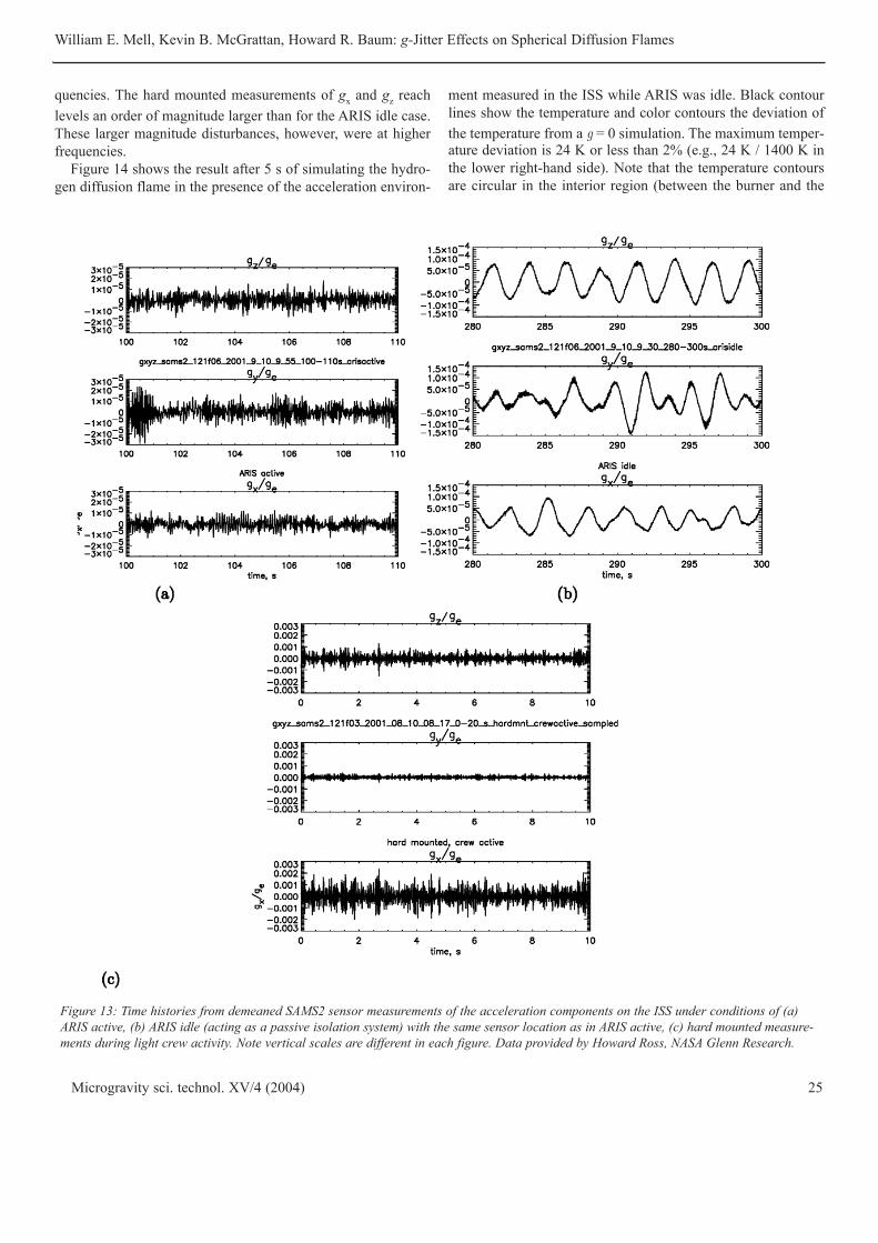
quencies. The hard mounted measurements of gx and gz reachlevels an order of magnitude larger than for the ARIS idle case.These larger magnitude disturbances, however, were at higherfrequencies.

Figure 14 shows the result after 5 s of simulating the hydro-gen diffusion flame in the presence of the acceleration environ-

ment measured in the ISS while ARIS was idle. Black contourlines show the temperature and color contours the deviation ofthe temperature from a g = 0 simulation. The maximum temper-ature deviation is 24 K or less than 2% (e.g., 24 K / 1400 K inthe lower right-hand side). Note that the temperature contoursare circular in the interior region (between the burner and the



Figure 13: Time histories from demeaned SAMS2 sensor measurements of the acceleration components on the ISS under conditions of (a)ARIS active, (b) ARIS idle (acting as a passive isolation system) with the same sensor location as in ARIS active, (c) hard mounted measure-ments during light crew activity. Note vertical scales are different in each figure. Data provided by Howard Ross, NASA Glenn Research.

flame) but elongated vertically in the outer region. This elonga-tion was due to the heating of the experimental support platformat the top of the figure (outlined by a 300 K contour line, alsosee Fig. 12). The platform was modeled as a thermally thicksolid. Since the platform was also present in the g = 0 simula-tions its affect on the temperature contours has been accountedfor when testing for the influence of g-jitter. The temperaturedeviations in this case were significantly smaller than those inthe previous experimental cases considered (e.g., free-floatingaircraft, Fig. 8). Simulations with g from Fig. 13(c) (no isolationsystem, light crew activity) had a similar magnitude of maxi-mum temperature deviation (not shown). Simulations with gfrom Fig. 13(a) (ARIS active) had maximum temperature devi-ations of 2 K.

7. Simulations using predicted acceleration disturbances on the ISS

Predictions of acceleration disturbances obtained from finiteelement simulations of the fully complete ISS structure operat-ing with all known sources of acceleration disturbance "turnedon" (e.g., control moment gyroscopes, ergometers, solar paneljoints) and without any isolation systems present are available.These acceleration disturbances are based on a Non IsolatedRack Assessment (NIRA) which is a prediction of the accelera-tion environment in Columbus Laboratory after completion ofthe ISS assembly and during the microgravity periods. The

NIRA sky line vibratory assessment includes the disturbancesources in the structural dynamic and vibro-acoustic range (0.01through 300 Hz) and results from Boeing/NASA-JSC models ofthe assembled ISS with the addition of forcing functions. Theanalysis assumes a 1% damping applied to the 100 second aver-aged, root-mean-square acceleration magnitude at the centerfrequencies of the one-third octave bands from 0.01 through300 Hz.

Figure 15 shows NIRA derived information of the accelera-tion environment in the ISS. Figure 15(a) is a spectral plot of theNIRA prediction of the magnitude of the acceleration. Figure15(b) is ten seconds of the acceleration time history obtained bya sum of sinusoids whose frequencies and amplitudes areobtained from a modification of the NIRA prediction in Fig.15(a). Note that the full range of frequencies covered by theNIRA prediction were not plotted in Fig. 15(a). Using higherfrequencies made little difference in the derived accelerationtime history since their amplitude was two orders of magnitudelower (not shown) than the 10-2 ge peak at approximately 3 Hzeasily seen in Fig. 15(a). Figure 15(c) shows (dotted line out to100 Hz) the portion of the original NIRA data in Fig. 15(a) thatwas actually used to compute the time series in Fig. 15(b). Thesolid line in Fig. 15(c) shows the result of using a Hanning fil-ter on the time history and then performing an FFT, computingthe power spectral density (PSD) and plotting its square root.The lower frequencies were lost due to the Hanning filter. At allother frequencies the square root of the PSD agree well with theoriginal NIRA data. The original NIRA data was damped for



Figure 14: Result three-dimensional adiabatic simulation of ahydrogen diffusion flame (60%H2-40%N2 by mole fraction,m·

FM=0.0081 g/s, 5 s into the simulation) in the GIFFTS apparatuswith a measured acceleration vector obtained when ARIS is idle onthe ISS (i.e., Fig. 13b the ARIS system was acting as a passive isola-tion system). Black contour lines show the temperature (K), colorcontours show the temperature deviation from a g = 0 simulation.The rectangular 300 K black contour at the top of the figure is dueto the experimental support platform (see Fig. 12).

Figure 15: Acceleration data derived from a NIRA prediction. (a) Aspectral plot of the NIRA prediction of the acceleration. (b) A 10 sacceleration time history derived from a modified form of the spec-tral data. (c) The portion of the original spectral data that was usedto compute the time series (dotted line out to 100 Hz). See the textfor more details. Data in Fig. (a) was provided by Marcus Just, ZinnTechnologies.

frequencies greater than 10 Hz because at the time of this runthe validity of the amplitudes at higher frequencies was in ques-tion. Also, frequencies higher than 100 Hz were cutoff. The rea-son for the 100 Hz cutoff is to avoid aliasing by the simulationcode which effectively samples the time history at 200 Hz. Notethat the 3 Hz peak, which was due to an ergometer, dominatesthe time history behavior in Fig. 15(b).

The level of peak acceleration disturbance (± 0.02ge at ≈ 3Hz) in Fig. 15(b) is comparable to bolted down experiments inthe DC-9 (see Fig. 9), and an order of magnitude larger than thehard mounted (light crew activity) case of Fig. 13. Note, how-ever, that the accelerations in the hard mounted case are at high-er frequencies. The peak disturbance also violates the limit foran oscillatory acceleration disturbance which is 48 micro-ge at 3Hz (see Sec. 2).

The time history in Fig. 15(b) was used to represent the gzcomponent of the acceleration vector, ge = (0, 0, gnira), in a sim-ulation of a spherical hydrogen diffusion flame (60%H2-40%N2

by mole fraction, m·FM =0.0081 g/s). The properties of the simu-

lation (i.e., grid resolution, etc.) were the same as the simula-tions conduction in Sec. 7 above. Note, however, that the simu-lations in Sec. 7 used measured acceleration data for all threecomponents of the acceleration vector. In Fig. 16 the results ofthe simulation using g = (0, 0,gnira) are plotted. The deviationfrom the g = 0 case is twice that of the other ISS cases consid-ered (ARIS idle, Fig. 14; hard mounted with light crew activity,not shown). In animations of the simulation the flame clearlyoscillated vertically as it spread outward from the burner.

In order to test whether the acceleration disturbance at 3 Hzwas the source of the flame's oscillatory behavior the peak wasremoved from the NIRA spectrum in Fig. 15(a) and a newacceleration time history was computed and used in the spheri-cal flame simulation. Figure 17(a) shows the original NIRA pre-diction and the dotted line in Fig. 17(c) shows its modified formwithout the peak at 3 Hz. This modified spectrum, out to 50 Hz,was used to obtain the acceleration time history shown in Fig.17(b). As before, this acceleration time history was used for thegz component of the the acceleration vector in a new simulation.No flame oscillation was observed in animations of the simula-tion. However, animations did clearly show the flame movingdownward. The source of this disturbance can be identified bychecking to see if the acceleration time history meets the crite-ria of a 10 micro-g seconds integrated disturbance. Figure 17(d)is a time history plot of the running sum:

As stated in Eq. (35) this running sum must be less than or equalto 1 0 micro-ge seconds over a time interval of 10 s or less. It is



Figure 16: Result three-dimensional adiabatic simulation of ahydrogen diffusion flame (60%H2-40%N2 by mole fraction, m·

FM=0.0081 g/s, 5 s into the simulation) in the GIFFTS apparatus withacceleration vector g = (0; 0; gNIRA) where gNIRA was obtained fromNIRA predictions and is plotted in Fig. 15. Black contour lines showthe temperature (K), color contours show the temperature deviationfrom a g = 0 simulation.

Figure 17: NIRA derived acceleration. (a) Original NIRA prediction.(b) Time series of acceleration derived from the modified NIRAspectrum of (c) using a sum of sines. (c) The original NIRA spec-trum in (a) with the ≈ 3 Hz peak is removed is shown as a dottedline. This spectrum out to 50 Hz was used to derive the time seriesin (b). (d) Running sum of the acceleration time series multiplied bydt in (b). This is a running check of whether or not the accelerationdisturbance meets the integrated transient disturbance limit. Notethat the vertical axis is in units of micro-ge.

010 micro seconds for 10 .

t NIRAe

e

gt g t s

g∆ ≤ − ≤∫ (35)

clear from Fig. 17(d) that the flame is subjected to a net accel-eration disturbance in the positive z direction. This disturbancedoes not meet the integrated transient limit requirement. Notethe vertical axis in Fig. 17(d) is in units of micro-ge. This unde-sirable integrated acceleration disturbance is the result of usinga sum of sines based on a spectrum which has a broad range offrequencies with amplitudes large enough to affect the flame. Inthe previous simulation case, because the 3 Hz peak in the mod-ified NIRA spectrum sufficiently dominated the accelerationtime history, this transient acceleration was not a relevant dis-turbance.

The results of this and the previous section suggest that a pas-sive isolation system and appropriate scheduling of crew andstation activity would provide a sufficiently "quiet" accelerationenvironment for spherical diffusion flame experiments.

8. Summary and Conclusions

A transient, three-dimensional, model for simulating laminarflames with a single hydrocarbon fuel was developed to assessthe influence of g-jitter. A requirement of the approach was thatit be computationally efficient so that it could be used by exper-imentalists as an aid to assessing g-jitter effects in a range ofexperimental scenarios. For this reason, and because it is a rea-sonable first step toward more sophisticated chemistry models(if needed), a mixture fraction based combustion model wasused. Based on the validation results of spherical diffusionflame simulations over a range of grid resolutions this modelperformed very well except under conditions in which differen-tial diffusion (which can not be accounted for by the mixturefraction based combustion model) was most relevant.

Numerical simulations of a spherical diffusion flame wereused to assess the validity of the recommended limit on inte-grated transient acceleration disturbances (see Sec. 2). Theresults suggested that the limit is valid (temperatures deviationsof less than 0.5% were caused by the disturbance) and couldeven be relaxed. A more thorough testing of all the recom-mended limits listed in Sec. 2 will be conducted in the future fora range of combustion problems including spherical diffusionflames, flame spread over a solid, and premixed flames.

Simulations were performed using g-jitter measured on theISS with an active, a passive, and no isolation system presentand as predicted by structural models of the fully complete ISS.Results from these simulations suggested that a passive isola-tion system with properly scheduled crew activity would pro-vide a suitably g-jitter free environment for spherical diffusionflames.

9. Acknowledgements

This work was funded by NASA under it's MicrogravityCombustion Research Program. The authors wish to thank Dr.Howard Ross, NASA Glenn Research Center, for providingvaluable guidance and acceleration data. Marcus Just of Zinn

Technologies provided the the original NIRA data in Figs. 15and 17. Collaborations with Drs. Peter Struk and DouglasFeikeman were also greatly appreciated.

10. Nonemclature

Variable Units Description

cp,mix kJ/kg·K specific heat of mixture at constant pressure

c_

p,mix kJ/kmole·K molar specific heat of mixture at constant pressure

cp,i kJ/kg·K specific heat of species i at constant pressure

cv,mix kJ/kg·K specific heat of mixture at constant volume

c_

v,i kJ/kmole·K molar specific heat of species i at constant volume

D = Dmix m/s2 mass diffusion coefficient of gaseous mixture

Di,mix m2/s mass diffusion coefficient of species iinto local mixture

f Hz frequency of g-jitter

g gram unit of mass

g = (gx, gy, gz) m/s2 ambient acceleration vector

gx, gy, gz m/s2 components of the ambient acceleration vector

ge = 9.8 m/s2 acceleration of gravity on Earth

gRMS m/s2 root-mean-square of acceleration vector

H - Heavyside function

H m2=s2 modified pressure term in momentum equation

hi kJ/kg specific enthalpy of species i

hoi kJ/kg specific enthalpy of formation species i

at reference temperature To

h = Σi Yi hi kJ/kg mixture enthalpy

h_

i = hiMi kJ/kmole molar specific enthalpy of species i

Iλ(χ,s) W·MHz/m2 · sr spectral radiation intensity

Ib,λ(χ,s) W·MHz/m2 · sr blackbody spectral radiation intensity

m· FM g/s mass flow rate of fuel mixture from burner

m· i’’’ kg=s · m3 chemical mass consumption of species i

Mi kg/kmole molecular weight of species i

M = (ΣiYi /Mi )-1 kg/kmole average molecular weight of gas mixture



Q· c’’’ kW/m³ heat release due to chemical reactions

Superscripts

’ derivative with respect to mixture fraction, ( )’ = d( ) / dZ

Variable Units Description

pd Pa dynamic pressure

po Pa thermodynamic pressure

R = 8.314 kJ/kmole·K universal gas constant·q”R,e kW/m2 thermal radiation flux

s - unit vector in direction of radiation intensity

u m/s velocity vector

χ m position vector

yi = MYi / Mi - mole fraction of species i

Yi = ρ i/ ρ - mass fraction of species i

Y∞F - mass fraction of fuel in fuel stream

Y∞O2 - mass fraction of oxygen in oxidant

Z - mixture fraction

Zst - stoichiometric value of the mixturefraction

γmix = (cp/ cv)mix - ratio of mixture specific heats

γi = cp,i = cv,,i - ration of species i specific heats

∆hc kJ/kmole molar based heat of combustion

η = Z/Zst - used as an argument for Heavyside function

∆hc kJ/kg mass based heat of combustion

∆χ mm grid cell size

λ µm wavelength of radiation, or

λ W/m·K thermal conductivity of the gaseous mixture

λi W/m·K thermal conductivity of species i

µ kg /m · s dynamic viscosity of the gaseous mixture

µi kg /m · s dynamic viscosity of species i

νi - stoichiometric coefficient of species i

ρ kg/m3 density of gaseous mixture

ρi kg/m3 density of species i

τ kg = m · s2 viscous stress tensor

Ω sr solid angle

Subscripts

F fuel species

O2 oxygen species

λ spectral dependence

11. References

[1] NASA SSP 410000 revision E, 1996. The Microgravity Plan, paragraph6.2.5.

[2] P.M. Struk, D.L. Dietrich, and J.S. T'ien. Large Droplet CombustionExperiment Using Porous Spheres Conducted in Reduced GravityAboard an Aircraft - Extinction and the Effects of g-jitter. MicrogravitySci. Technol., 9(2):106116, 1996.

[3] D. Feikema. Effects of Acceleration Environment on the Stability ofSpherical Diffusion Flames. In Second Joint Meeting of the U.S.Sections of the Combustion Institute. The Combustion Institute, March26-27, Oakland, CA 2001.

[4] S. Ostrach. Natural convection with combined driving forces.Pysiochemical Hydrodynamics, 1:233-247, 1980.

[5] S. Ostrach. Low-Gravity °uid °ows. Ann. Rev. Fluid Mech., 14:313-345,1982.

[6] Y. Kamotani, A. Prasad, and S. Ostrach. Thermal convection in an enclo-sure due to vibrations aboard a spacecraft. AIAA Journal, 19:511-516,1981.

[7] C.R. Kaplan, E.S. Oran, K. Kailasanath, and H.D. Ross. Gravitationaleffect on sooting diffusion flames. Proceedings of the CombustionInstitute, 26:1301-1309, 1996.

[8] M. Long, K. Walsh, and M. Smooke. Computational and ExperimentalStudy of Laminar Diffusion Flames in a Microgravity Environment.pages 123-128. Cleveland, OH, Proceedings of the Fourth InternationalMicrogravity Combustion Workshop, May 19-21 1997.

[9] S.D. Tse, D.L. Zhu, C.J. Sung, and C.K. Law. Microgravity Burner-Generated Spherical Diffusion Flames: Experiment and Computation.AIAA Aerospace Sciences Meeting and Exhibit, AIAA-99-0585, 1999.

[10] S.D. Tse, D.L. Zhu, C.J. Sung, and C.K. Law. Microgravity Burner-Generated Spherical Diffusion Flames: Experiment and Computation.Combustion and Flame, 125:1265-1278, 2001.

[11] R.G. Rehm and H.R. Baum. The Equations of Motion for ThermallyDriven, Buoyant Flows. Journal of Research of the NBS, 83:297-308,1978.

[12] K.B. McGrattan, H.R. Baum, R.G. Rehm, A. Hamins, G.P. Forney, J.E.Floyd, S. Hostikka, and K. Prasad. Fire Dynamics Simulator, TechnicalReference Guide. Technical Report NIS-TIR 6782, 2002 Ed., NationalInstitute of Standards and Technology, Gaithersburg, Maryland,November 2002. http://fire.nist.gov/bfrlpubs/.

[13] D.E. Rosner. Transport Processes in Chemically Reacting Flow Systems.Dover Publications, Inc., Mineola, New York, 2000.

[14] G.D. Raithby and E.H. Chui. A Finite-Volume Method for PredictingRadiant Heat Transfer in Enclosures with Participating Media. J. HeatTransfer, 112(2):415-423, 1990.

[15] W. Grosshandler. RadCal: A Narrow Band Model for RadiationCalculations in a Combustion Environment. Technical Report TN 1402,National Institute of Standards and Technology, 1993.

[16] J.B. Bell, N.J. Brown, M.S. Day, M. Frenklach, J.F. Grcar, and S.R Tonse.The Dependence of Chemistry on the Inlet Equivalence Ratio in Vortex-Flame Interactions. Proc. Combustion Inst., 28:1933-1939, 2000.

[17] B.E. Poling, J.M. Prausnitz, and O'Connel J.P. Properties of Gases andLiquids. McGraw-Hill, Inc., New York, 5th edition, 2001.

[18] S.D. Tse, Rutgers, State University of New Jersey, personal communica-tion, 2003.

[19] E. Baumann, NASA Glenn Research Center, personal communication,2003.

[20] K. Miyasak and C.K. Law. Combustion of strongly-interacting lineardroplet arrays. Proc. Combust. Inst., 18:282-292, 1981.

[21] H. Ross, B. Espinoza, NASA Glenn Research Center, personal communi-



cation 1999, and also see. “Flame spread across liquids" in theProceedings of the Fourth International Microgravity CombustionWorkshop, May 19-21, 1997, Cleveland, OH, pp. 375-380.

[22] R. Delombard. Compendeum of Information of Interpreting theMicrogravity Environment of the Orbiter Spacecraft. Technical report,NASA Lewis Research Center, Cleveland, OH, 1996. NASA TechnicalMemorandum 107032.

[23] L.G. Blevins. Behavior of bare and aspirated thermocouples in compart-ment fires. In Proceedings of the 33rd National Heat Transfer



g-Jitter effects on spherical diffusion flames

Documents

Transcript of g-Jitter effects on spherical diffusion flames