Generating Similar Graphs From Spherical Features

GENERATING SIMILAR GRAPHS FROM SPHERICALFEATURES

Dalton Lunga and Sergey Kirshner{dlunga,skirshne}@purdue.edu

Purdue University

Department of Statistics

West Lafayette, IN 47907-2035 USA

www.purdue.edu/stat

May 12 2011

Technical Report No 11-01

arX

iv:1

105.

2965

v2 [

cs.S

I] 1

9 M

ay 2

011

Summary

We propose a novel model for generating graphs similar to a given example graph.Unlike standard approaches that compute features of graphs in Euclidean space, ourapproach obtains features on a surface of a hypersphere. We then utilize a von Mises-Fisher distribution, an exponential family distribution on the surface of a hypersphere,to define a model over possible feature values. While our approach bears similarityto a popular exponential random graph model (ERGM), unlike ERGMs, it does notsuffer from degeneracy, a situation when a significant probability mass is placed onunrealistic graphs. We propose a parameter estimation approach for our model, anda procedure for drawing samples from the distribution. We evaluate the performanceof our approach both on the small domain of all 8-node graphs as well as largerreal-world social networks.

i

Contents

1 Introduction 1

2 ERGMs 22.1 ERGM Definition . . . . . . . . . . . . . . . . . . . . . . . . . . . . . 22.2 Degeneracy in ERGMs . . . . . . . . . . . . . . . . . . . . . . . . . . 42.3 Why Are Unrealistic Graphs Likely under ERGMs? . . . . . . . . . . 6

3 Exponential Locally Spherical Random Graph Model 103.1 Algorithm . . . . . . . . . . . . . . . . . . . . . . . . . . . . . . . . . 103.2 Sampling under ELSRGM . . . . . . . . . . . . . . . . . . . . . . . . 12

4 Experimental Evaluation 144.1 Small graphs . . . . . . . . . . . . . . . . . . . . . . . . . . . . . . . 164.2 Larger Graphs . . . . . . . . . . . . . . . . . . . . . . . . . . . . . . . 16

5 Conclusion and Future Work 17

6 Acknowledgements 19

ii

List of Figures

1 Simple typical subgraph configurations for undirected graphs. Fromleft to right : edge, triangle, two-star and three-star configurations. 3

2 left: Distribution of 8-node graphs. right: Distribution of cell diameter;where we consider each feature-pair as a cell and compute the graphedit distance between each pair of graphs with feature counts mappingto that cell (feature-pair). . . . . . . . . . . . . . . . . . . . . . . . . 5

3 A degenerate ERGM specified by edge-triangle pair for an 8-nodegraph(top figure). Colorcoded is the pmf over the edge-triangle spacefor an estimated MLE θMLE = (−0.992, 0.617). ”+” indicates the ob-served feature and its mean, while the ”�” shape indicates the ERGMmode. . . . . . . . . . . . . . . . . . . . . . . . . . . . . . . . . . . . 6

4 Solid points show mode placement on the edge-triangle feature pairsthat form the vertices of the extended hull as a result of Theorem 1.Overlayed on solid points are modes obtained from using the estimatedθmle of equation (3). . . . . . . . . . . . . . . . . . . . . . . . . . . . 7

5 View of mode placement on facets of the extended 3D convex hull.Each mode forms a vertex of a given triangle (denoted by black lines)for a facet of the convex hull. . . . . . . . . . . . . . . . . . . . . . . 8

6 An illustration of degeneracy of exponential models on non-graph data.Colorcoded is the pmf over 2D grid spaces for estimated MLEs (leftplot) θMLE = (−0.086, 0.086) & (right plot) θMLE = (0.120,−0.160).”+” sign indicates the observed feature and its mean, while the ”�”shape indicates ERGM mode. . . . . . . . . . . . . . . . . . . . . . . 9

7 Two 8-node synthetic test graphs. Left: 2-component graph Gtest1

falling inside the relative interior of the convex hull C of extendedfeatures. Right: Gtest2 falling on the relative boundary of the convexhull C for the extended feature space. . . . . . . . . . . . . . . . . . . 17

8 Sample KL-divergence KL(f ‖ f

)for ELSRGM as more graphs get

uncovered. The initial neighborhood B ⊂ Gn(n = 8) is built aroundGtest1. . . . . . . . . . . . . . . . . . . . . . . . . . . . . . . . . . . . 17

9 (a) Synthetic graph Gtest1 ; (b) Corresponding feature-pair: f(Gtest1) ∈rint

(C); (c) Simulations from models given Gtest1 . The observed statis-

tics are indicated by the solid lines; the box plots include the medianand interquartile range of simulated networks. ERGMs show low vari-ance and all 100 samples seem to be placed on the same network- signof degeneracy. . . . . . . . . . . . . . . . . . . . . . . . . . . . . . . . 18

10 (a) Synthetic graph Gtest2 ; (b) Corresponding feature-pair: f(Gtest2) ∈rbd

(C); (c) Simulations from models given Gtest2 . The observed statis-

tics are indicated by the solid lines; the box plots include the medianand interquartile range of simulated networks. Both models are non-degenerate. . . . . . . . . . . . . . . . . . . . . . . . . . . . . . . . . 19

iii

11 Dolphin 62-node network summaries. The observed statistics are in-dicated by the solid lines; the box plots include the median and in-terquartile range of simulated networks. ERGM plots shows signs ofdegeneracy effect. . . . . . . . . . . . . . . . . . . . . . . . . . . . . . 20

12 Faux-Mesa-High 205-node network summaries. The observed statisticsare indicated by the solid lines; box plots summarize the statistics forthe simulated networks. ERGM plots shows signs of degeneracy effect. 20

13 Kapferer’s 39-node network summaries. The observed statistics areindicated by the solid lines; box plots summarize the statistics for thesimulated networks using ELSRGM. . . . . . . . . . . . . . . . . . . . . 20

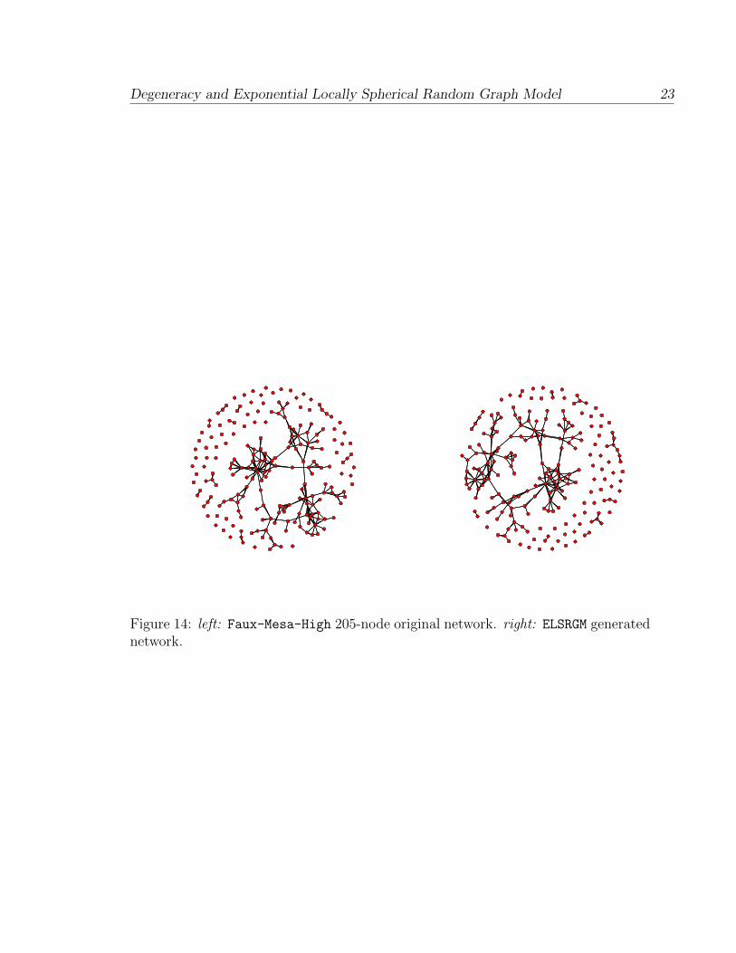
14 left: Faux-Mesa-High 205-node original network. right: ELSRGM gen-erated network. . . . . . . . . . . . . . . . . . . . . . . . . . . . . . . 23

iv

List of Tables

1 Complexity of graph spaces for fixed number of nodes. . . . . . . . . 4

v

Degeneracy and Exponential Locally Spherical Random Graph Model 1

1 Introduction

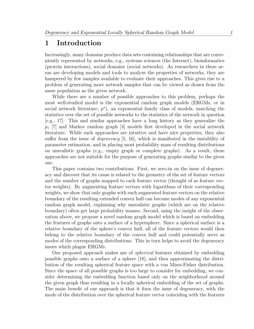
Increasingly, many domains produce data sets containing relationships that are conve-niently represented by networks, e.g., systems sciences (the Internet), bioinformatics(protein interactions), social domains (social networks). As researchers in these ar-eas are developing models and tools to analyze the properties of networks, they arehampered by few samples available to evaluate their approaches. This gives rise to aproblem of generating more network samples that can be viewed as drawn from thesame population as the given network.

While there are a number of possible approaches to this problem, perhaps themost well-studied model is the exponential random graph models (ERGMs, or insocial network literature, p?), an exponential family class of models, matching thestatistics over the set of possible networks to the statistics of the network in question[e.g., 17]. This and similar approaches have a long history as they generalize thep1 [7] and Markov random graph [4] models first developed in the social networkliterature. While such approaches are intuitive and have nice properties, they alsosuffer from the issue of degeneracy [5, 16], which is manifested in the instability ofparameter estimation, and in placing most probability mass of resulting distributionson unrealistic graphs (e.g., empty graph or complete graphs). As a result, theseapproaches are not suitable for the purpose of generating graphs similar to the givenone.

This paper contains two contributions. First, we zero-in on the issue of degener-acy and discover that its cause is related to the geometry of the set of feature vectorsand the number of graphs mapped to each feature vector (thought of as feature vec-tor weights). By augmenting feature vectors with logarithms of their correspondingweights, we show that only graphs with such augmented feature vectors on the relativeboundary of the resulting extended convex hull can become modes of any exponentialrandom graph model, explaining why unrealistic graphs (which are on the relativeboundary) often get large probability masses. Second, using the insight of the obser-vation above, we propose a novel random graph model which is based on embeddingthe features of graphs onto a surface of a hypersphere. Since a spherical surface is arelative boundary of the sphere’s convex hull, all of the feature vectors would thenbelong to the relative boundary of the convex hull and could potentially serve asmodes of the corresponding distributions. This in turn helps to avoid the degeneracyissues which plague ERGMs.

Our proposed approach makes use of spherical features obtained by embeddingpossible graphs onto a surface of a sphere [18], and then approximating the distri-bution of the resulting spherical feature space with a von Mises-Fisher distribution.Since the space of all possible graphs is too large to consider for embedding, we con-sider determining the embedding function based only on the neighborhood aroundthe given graph thus resulting in a locally spherical embedding of the set of graphs.The main benefit of our approach is that it fixes the issue of degeneracy, with themode of the distribution over the spherical feature vector coinciding with the features


of the given graph. An additional advantage of our approach is that its parameter es-timation procedure does not require cumbersome maximum entropy approaches usedwith ERGMs.

We start by revisiting the ERGM model and presenting insights on why this modeloften fails to generate realistic graphs (Section 2). We then propose our alternativeapproach, exponential locally spherical random graph model (ELSRGM, Section 3) andevaluate it on both synthetic and realistic graphs while comparing it to ERGMs(Section 4). We conclude the paper (Section 5) with ideas for future work.

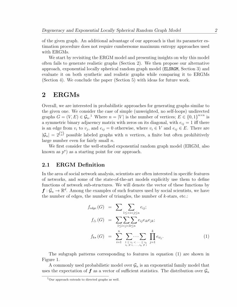
2 ERGMs

Overall, we are interested in probabilistic approaches for generating graphs similar tothe given one. We consider the case of simple (unweighted, no self-loops) undirectedgraphs G = (V,E) ∈ Gn.1 Where n = |V | is the number of vertices; E ∈ {0, 1}n×n isa symmetric binary adjacency matrix with zeros on its diagonal, with eij = 1 iff thereis an edge from vi to vj, and eij = 0 otherwise, where vi ∈ V and eij ∈ E. There are

|Gn| = 2(n2) possible labeled graphs with n vertices, a finite but often prohibitively

large number even for fairly small n.We first consider the well-studied exponential random graph model (ERGM, also

known as p?) as a starting point for our approach.

2.1 ERGM Definition

In the area of social network analysis, scientists are often interested in specific featuresof networks, and some of the state-of-the-art models explicitly use them to definefunctions of network sub-structures. We will denote the vector of these functions byf : Gn → Rd. Among the examples of such features used by social scientists, we havethe number of edges, the number of triangles, the number of k-stars, etc.:

fedge (G) =∑ ∑

1≤<i<j≤n

eij;

f4 (G) =∑∑∑1≤i<j<k≤n

eijeikejk;

fk? (G) =n∑i=1

∑· · ·∑

1 ≤ i1 < · · · ≤ iki1 6= i, . . . , ik 6= i

k∏j=1

eiij . (1)

The subgraph patterns corresponding to features in equation (1) are shown inFigure 1.

A commonly used probabilistic model over Gn is an exponential family model thatuses the expectation of f as a vector of sufficient statistics. The distribution over Gn

1Our approach extends to directed graphs as well.


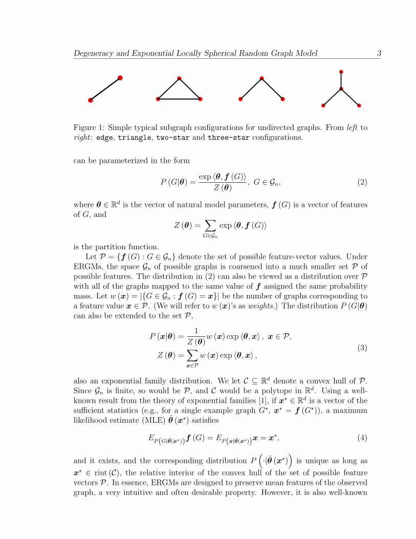
Figure 1: Simple typical subgraph configurations for undirected graphs. From left toright : edge, triangle, two-star and three-star configurations.

can be parameterized in the form

P (G|θ) =exp 〈θ,f (G)〉

Z (θ), G ∈ Gn, (2)

where θ ∈ Rd is the vector of natural model parameters, f (G) is a vector of featuresof G, and

Z (θ) =∑G∈Gn

exp 〈θ,f (G)〉

is the partition function.Let P = {f (G) : G ∈ Gn} denote the set of possible feature-vector values. Under

ERGMs, the space Gn of possible graphs is coarsened into a much smaller set P ofpossible features. The distribution in (2) can also be viewed as a distribution over Pwith all of the graphs mapped to the same value of f assigned the same probabilitymass. Let w (x) = |{G ∈ Gn : f (G) = x}| be the number of graphs corresponding toa feature value x ∈ P . (We will refer to w (x)’s as weights.) The distribution P (G|θ)can also be extended to the set P ,

P (x|θ) =1

Z (θ)w (x) exp 〈θ,x〉 , x ∈ P ,

Z (θ) =∑x∈P

w (x) exp 〈θ,x〉 ,(3)

also an exponential family distribution. We let C ⊆ Rd denote a convex hull of P .Since Gn is finite, so would be P , and C would be a polytope in Rd. Using a well-known result from the theory of exponential families [1], if x? ∈ Rd is a vector of thesufficient statistics (e.g., for a single example graph G?, x? = f (G?)), a maximumlikelihood estimate (MLE) θ (x?) satisfies

EP(G|θ(x?))f (G) = EP(x|θ(x?))x = x?, (4)

and it exists, and the corresponding distribution P(·|θ (x?)

)is unique as long as

x? ∈ rint (C), the relative interior of the convex hull of the set of possible featurevectors P . In essence, ERGMs are designed to preserve mean features of the observedgraph, a very intuitive and often desirable property. However, it is also well-known


that the estimation of θ (x?) is an extremely cumbersome task, complicated by thefact that the exact calculation of Z (θ) is intractable, and approximate approaches(e.g., pseudo-likelihood, MCMC) are employed instead [9].

2.2 Degeneracy in ERGMs

ERGMs often suffer from the problem of degeneracy [5]. There are two types ofdegeneracy usually considered. The first type occurs when the MLE estimate θ (x?)either does not exist, or the MLE estimation procedure does not converge due tonumerical instabilities [5, 16].

The second type of degeneracy happens when θ (x?) can be reliably estimated, butthe resulting probability distribution places significant probability mass (or virtuallyall of probability mass) on unrealistic graphs, e.g., empty or complete graphs. Thistype of degeneracy can be considered from another viewpoint; that is the mode ofERGM corresponding to the θ (x?) may be placed on x ∈ P very different fromx?. This is an undesirable property as there is little justification for placing largeprobability mass over a region away from observed feature vectors while placing littlemass over the observed example.

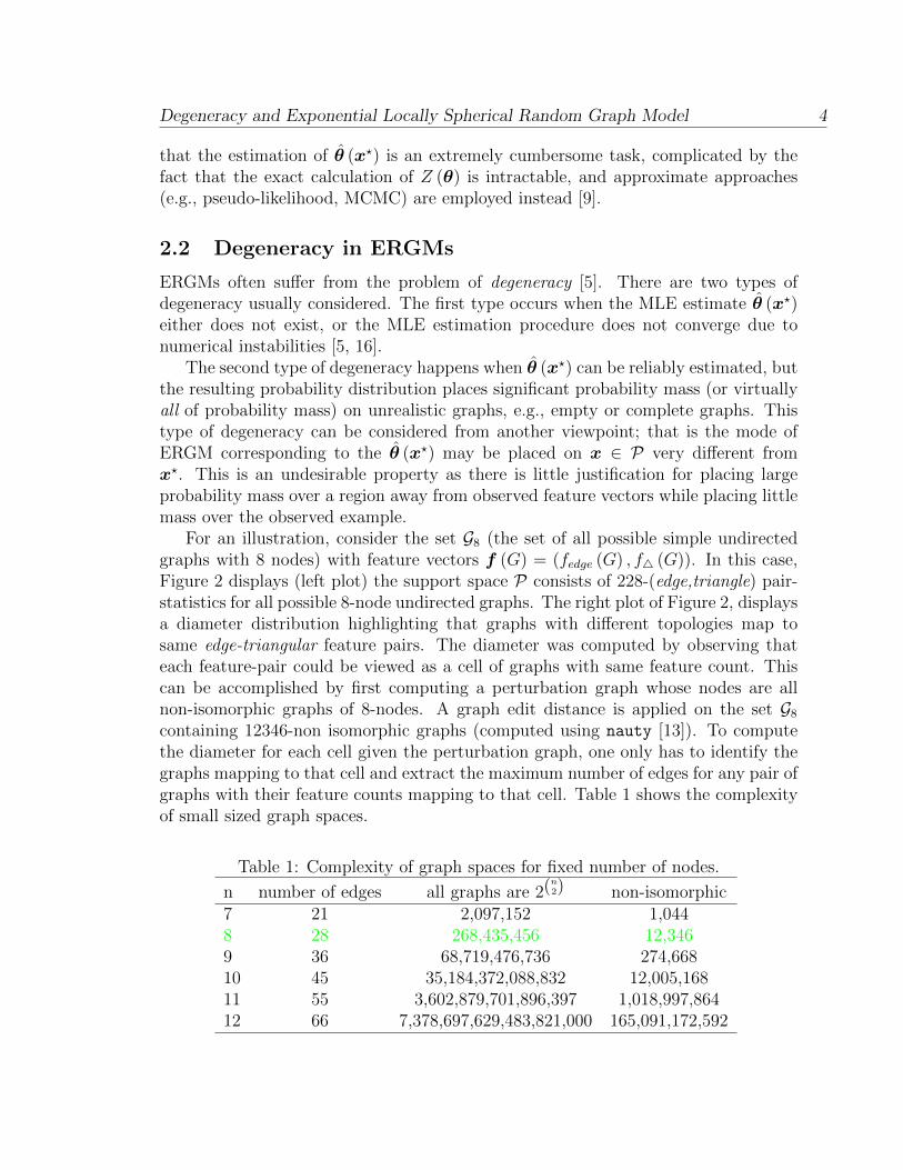
For an illustration, consider the set G8 (the set of all possible simple undirectedgraphs with 8 nodes) with feature vectors f (G) = (fedge (G) , f4 (G)). In this case,Figure 2 displays (left plot) the support space P consists of 228-(edge,triangle) pair-statistics for all possible 8-node undirected graphs. The right plot of Figure 2, displaysa diameter distribution highlighting that graphs with different topologies map tosame edge-triangular feature pairs. The diameter was computed by observing thateach feature-pair could be viewed as a cell of graphs with same feature count. Thiscan be accomplished by first computing a perturbation graph whose nodes are allnon-isomorphic graphs of 8-nodes. A graph edit distance is applied on the set G8containing 12346-non isomorphic graphs (computed using nauty [13]). To computethe diameter for each cell given the perturbation graph, one only has to identify thegraphs mapping to that cell and extract the maximum number of edges for any pair ofgraphs with their feature counts mapping to that cell. Table 1 shows the complexityof small sized graph spaces.

Table 1: Complexity of graph spaces for fixed number of nodes.

n number of edges all graphs are 2(n2) non-isomorphic

7 21 2,097,152 1,0448 28 268,435,456 12,3469 36 68,719,476,736 274,66810 45 35,184,372,088,832 12,005,16811 55 3,602,879,701,896,397 1,018,997,86412 66 7,378,697,629,483,821,000 165,091,172,592


0 5 10 15 20 25 300

10

20

30

40

50

60

number of edges

nu

mb

er o

f tr

ian

gle

s

6720

13440

20160

26880

33600

40320

0 5 10 15 20 25 300

10

20

30

40

50

60

number of edges

nu

mb

er o

f tr

ian

gle

s

0

2

4

6

8

10

12

Figure 2: left: Distribution of 8-node graphs. right: Distribution of cell diameter;where we consider each feature-pair as a cell and compute the graph edit distancebetween each pair of graphs with feature counts mapping to that cell (feature-pair).

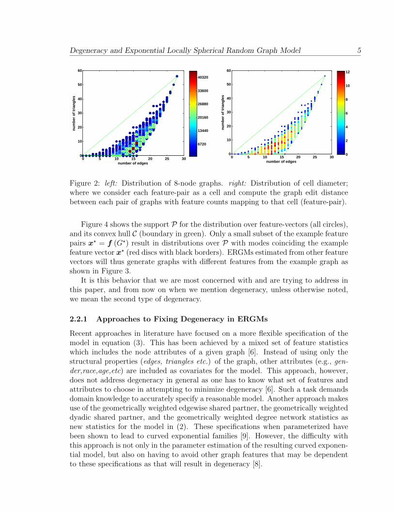
Figure 4 shows the support P for the distribution over feature-vectors (all circles),and its convex hull C (boundary in green). Only a small subset of the example featurepairs x? = f (G?) result in distributions over P with modes coinciding the examplefeature vector x? (red discs with black borders). ERGMs estimated from other featurevectors will thus generate graphs with different features from the example graph asshown in Figure 3.

It is this behavior that we are most concerned with and are trying to address inthis paper, and from now on when we mention degeneracy, unless otherwise noted,we mean the second type of degeneracy.

2.2.1 Approaches to Fixing Degeneracy in ERGMs

Recent approaches in literature have focused on a more flexible specification of themodel in equation (3). This has been achieved by a mixed set of feature statisticswhich includes the node attributes of a given graph [6]. Instead of using only thestructural properties (edges, triangles etc.) of the graph, other attributes (e.g., gen-der,race,age,etc) are included as covariates for the model. This approach, however,does not address degeneracy in general as one has to know what set of features andattributes to choose in attempting to minimize degeneracy [6]. Such a task demandsdomain knowledge to accurately specify a reasonable model. Another approach makesuse of the geometrically weighted edgewise shared partner, the geometrically weighteddyadic shared partner, and the geometrically weighted degree network statistics asnew statistics for the model in (2). These specifications when parameterized havebeen shown to lead to curved exponential families [9]. However, the difficulty withthis approach is not only in the parameter estimation of the resulting curved exponen-tial model, but also on having to avoid other graph features that may be dependentto these specifications as that will result in degeneracy [8].


0 10 20 300

10

20

30

40

50

60

number of edges

nu

mb

er o

f tr

ian

gle

s

0.000

0.005

0.010

0.015

0.019

0.024

0.029

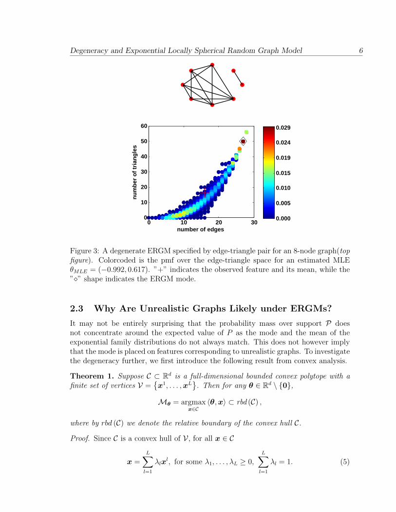
Figure 3: A degenerate ERGM specified by edge-triangle pair for an 8-node graph(topfigure). Colorcoded is the pmf over the edge-triangle space for an estimated MLEθMLE = (−0.992, 0.617). ”+” indicates the observed feature and its mean, while the”�” shape indicates the ERGM mode.

2.3 Why Are Unrealistic Graphs Likely under ERGMs?

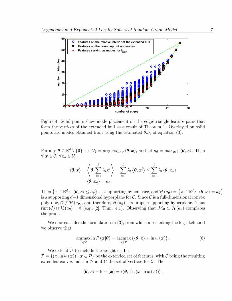
It may not be entirely surprising that the probability mass over support P doesnot concentrate around the expected value of P as the mode and the mean of theexponential family distributions do not always match. This does not however implythat the mode is placed on features corresponding to unrealistic graphs. To investigatethe degeneracy further, we first introduce the following result from convex analysis.

Theorem 1. Suppose C ⊂ Rd is a full-dimensional bounded convex polytope with afinite set of vertices V =

{x1, . . . ,xL

}. Then for any θ ∈ Rd \ {0},

Mθ = argmaxx∈C

〈θ,x〉 ⊂ rbd (C) ,

where by rbd (C) we denote the relative boundary of the convex hull C.

Proof. Since C is a convex hull of V , for all x ∈ C

x =L∑l=1

λlxl, for some λ1, . . . , λL ≥ 0,

L∑l=1

λl = 1. (5)


0 5 10 15 20 25 300

10

20

30

40

50

60

number of edges

nu

mb

er o

f tr

ian

gle

s

Features on the relative interior of the extended hullFeatures on the boundary but not modesFeatures serving as modes for θ

MLE

Figure 4: Solid points show mode placement on the edge-triangle feature pairs thatform the vertices of the extended hull as a result of Theorem 1. Overlayed on solidpoints are modes obtained from using the estimated θmle of equation (3).

For any θ ∈ Rd \ {0}, let Vθ = argmaxx∈V 〈θ,x〉, and let aθ = maxx∈V 〈θ,x〉. Then∀ x ∈ C, ∀xθ ∈ Vθ

〈θ,x〉 =

⟨θ,

L∑l=1

λlxl

⟩=

L∑l=1

λl⟨θ,xl

⟩≤

L∑l=1

λl 〈θ,xθ〉

= 〈θ,xθ〉 = aθ.

Then{x ∈ Rd : 〈θ,x〉 ≤ aθ

}is a supporting hyperspace, andH (aθ) =

{x ∈ Rd : 〈θ,x〉 = aθ

}is a supporting d−1 dimensional hyperplane for C. Since C is a full-dimensional convexpolytope, C 6⊂ H (aθ), and therefore, H (aθ) is a proper supporting hyperplane. Thusrint (C) ∩ H (aθ) = ∅ (e.g., [2], Thm. 4.1). Observing that Mθ ⊂ H (aθ) completesthe proof.

We now consider the formulation in (3), from which after taking the log-likelihoodwe observe that

argmaxx∈P

lnP (x|θ) = argmaxx∈P

{〈θ,x〉+ lnw (x)} . (6)

We extend P to include the weight w. LetP = {(x, lnw (x)) : x ∈ P} be the extended set of features, with C being the resultingextended convex hull for P and V the set of vertices for C. Then

〈θ,x〉+ lnw (x) = 〈(θ, 1) , (x, lnw (x))〉 .


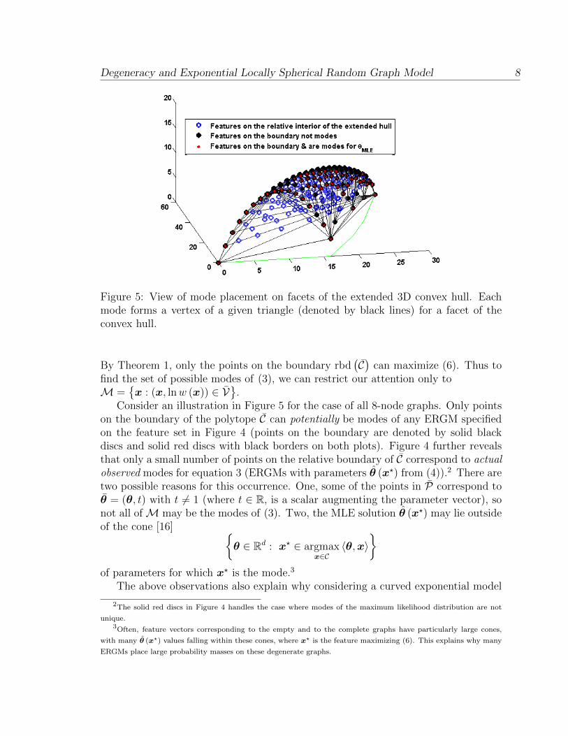
Figure 5: View of mode placement on facets of the extended 3D convex hull. Eachmode forms a vertex of a given triangle (denoted by black lines) for a facet of theconvex hull.

By Theorem 1, only the points on the boundary rbd(C)

can maximize (6). Thus tofind the set of possible modes of (3), we can restrict our attention only toM =

{x : (x, lnw (x)) ∈ V

}.

Consider an illustration in Figure 5 for the case of all 8-node graphs. Only pointson the boundary of the polytope C can potentially be modes of any ERGM specifiedon the feature set in Figure 4 (points on the boundary are denoted by solid blackdiscs and solid red discs with black borders on both plots). Figure 4 further revealsthat only a small number of points on the relative boundary of C correspond to actualobserved modes for equation 3 (ERGMs with parameters θ (x?) from (4)).2 There aretwo possible reasons for this occurrence. One, some of the points in P correspond toθ = (θ, t) with t 6= 1 (where t ∈ R, is a scalar augmenting the parameter vector), sonot all ofM may be the modes of (3). Two, the MLE solution θ (x?) may lie outsideof the cone [16] {

θ ∈ Rd : x? ∈ argmaxx∈C

〈θ,x〉}

of parameters for which x? is the mode.3

The above observations also explain why considering a curved exponential model

2The solid red discs in Figure 4 handles the case where modes of the maximum likelihood distribution are not

unique.3Often, feature vectors corresponding to the empty and to the complete graphs have particularly large cones,

with many θ (x?) values falling within these cones, where x? is the feature maximizing (6). This explains why many

ERGMs place large probability masses on these degenerate graphs.


[8]

P (x|θ) =1

Z (θ)w (x) exp 〈g (θ) ,x〉 , x ∈ P

does not rectify the issue of degeneracy as curving the space of parameters does notchange the geometry of the feature space.4

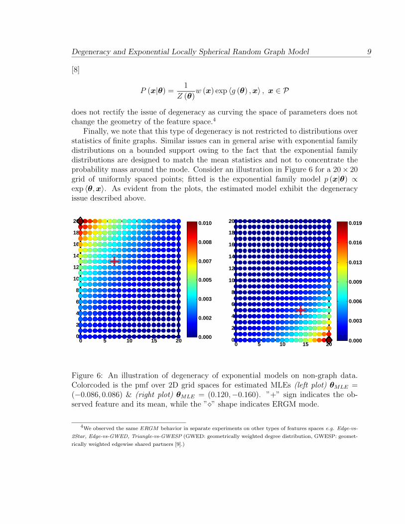
Finally, we note that this type of degeneracy is not restricted to distributions overstatistics of finite graphs. Similar issues can in general arise with exponential familydistributions on a bounded support owing to the fact that the exponential familydistributions are designed to match the mean statistics and not to concentrate theprobability mass around the mode. Consider an illustration in Figure 6 for a 20× 20grid of uniformly spaced points; fitted is the exponential family model p (x|θ) ∝exp 〈θ,x〉. As evident from the plots, the estimated model exhibit the degeneracyissue described above.

0 5 10 15 200

2

4

6

8

10

12

14

16

18

20

0.000

0.002

0.003

0.005

0.007

0.008

0.010

0 5 10 15 200

2

4

6

8

10

12

14

16

18

20

0.000

0.003

0.006

0.009

0.013

0.016

0.019

Figure 6: An illustration of degeneracy of exponential models on non-graph data.Colorcoded is the pmf over 2D grid spaces for estimated MLEs (left plot) θMLE =(−0.086, 0.086) & (right plot) θMLE = (0.120,−0.160). ”+” sign indicates the ob-served feature and its mean, while the ”�” shape indicates ERGM mode.

4We observed the same ERGM behavior in separate experiments on other types of features spaces e.g. Edge-vs-

2Star, Edge-vs-GWED, Triangle-vs-GWESP (GWED: geometrically weighted degree distribution, GWESP: geomet-

rically weighted edgewise shared partners [9].)


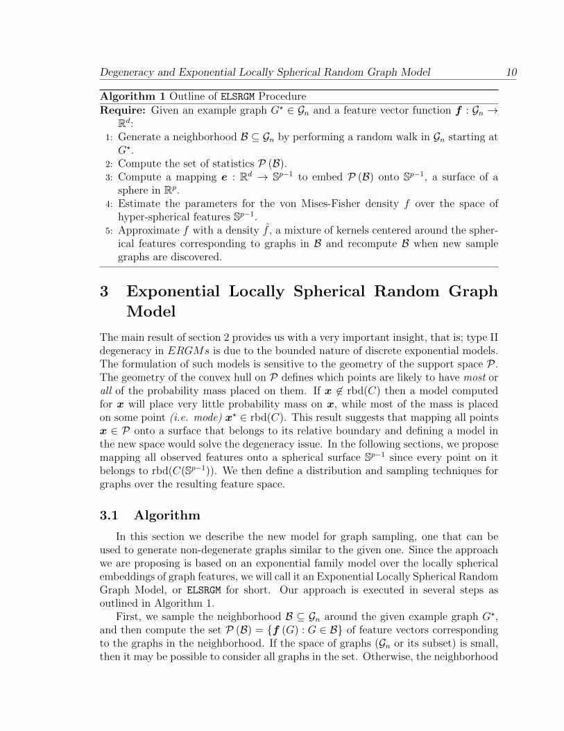
Algorithm 1 Outline of ELSRGM Procedure

Require: Given an example graph G? ∈ Gn and a feature vector function f : Gn →Rd:

1: Generate a neighborhood B ⊆ Gn by performing a random walk in Gn starting atG?.

2: Compute the set of statistics P (B).3: Compute a mapping e : Rd → Sp−1 to embed P (B) onto Sp−1, a surface of a

sphere in Rp.4: Estimate the parameters for the von Mises-Fisher density f over the space of

hyper-spherical features Sp−1.5: Approximate f with a density f , a mixture of kernels centered around the spher-

ical features corresponding to graphs in B and recompute B when new samplegraphs are discovered.

3 Exponential Locally Spherical Random Graph

Model

The main result of section 2 provides us with a very important insight, that is; type IIdegeneracy in ERGMs is due to the bounded nature of discrete exponential models.The formulation of such models is sensitive to the geometry of the support space P .The geometry of the convex hull on P defines which points are likely to have most orall of the probability mass placed on them. If x 6∈ rbd(C) then a model computedfor x will place very little probability mass on x, while most of the mass is placedon some point (i.e. mode) x? ∈ rbd(C). This result suggests that mapping all pointsx ∈ P onto a surface that belongs to its relative boundary and defining a model inthe new space would solve the degeneracy issue. In the following sections, we proposemapping all observed features onto a spherical surface Sp−1 since every point on itbelongs to rbd(C(Sp−1)). We then define a distribution and sampling techniques forgraphs over the resulting feature space.

3.1 Algorithm

In this section we describe the new model for graph sampling, one that can beused to generate non-degenerate graphs similar to the given one. Since the approachwe are proposing is based on an exponential family model over the locally sphericalembeddings of graph features, we will call it an Exponential Locally Spherical RandomGraph Model, or ELSRGM for short. Our approach is executed in several steps asoutlined in Algorithm 1.

First, we sample the neighborhood B ⊆ Gn around the given example graph G?,and then compute the set P (B) = {f (G) : G ∈ B} of feature vectors correspondingto the graphs in the neighborhood. If the space of graphs (Gn or its subset) is small,then it may be possible to consider all graphs in the set. Otherwise, the neighborhood


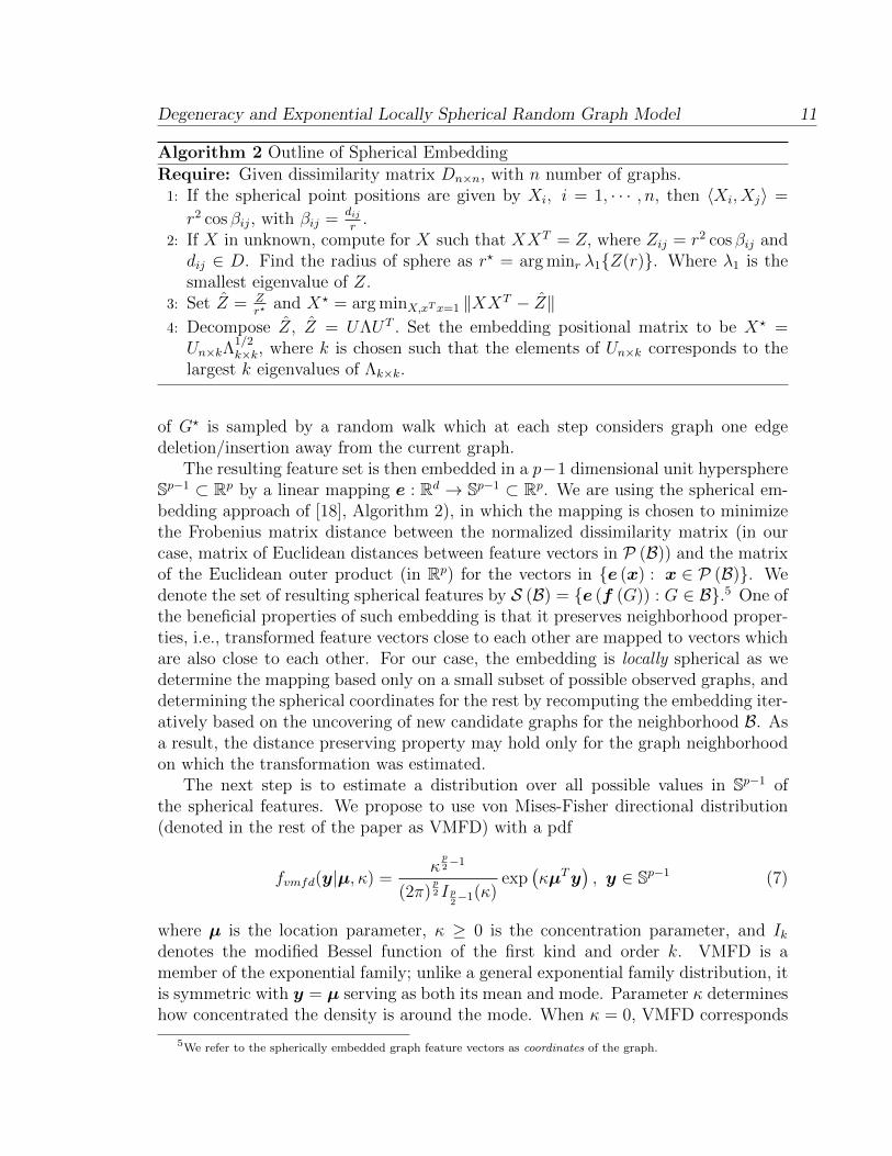
Algorithm 2 Outline of Spherical Embedding

Require: Given dissimilarity matrix Dn×n, with n number of graphs.1: If the spherical point positions are given by Xi, i = 1, · · · , n, then 〈Xi, Xj〉 =

r2 cos βij, with βij =dijr.

2: If X in unknown, compute for X such that XXT = Z, where Zij = r2 cos βij anddij ∈ D. Find the radius of sphere as r? = arg minr λ1{Z(r)}. Where λ1 is thesmallest eigenvalue of Z.

3: Set Z = Zr?

and X? = arg minX,xT x=1 ‖XXT − Z‖4: Decompose Z, Z = UΛUT . Set the embedding positional matrix to be X? =Un×kΛ

1/2k×k, where k is chosen such that the elements of Un×k corresponds to the

largest k eigenvalues of Λk×k.

of G? is sampled by a random walk which at each step considers graph one edgedeletion/insertion away from the current graph.

The resulting feature set is then embedded in a p−1 dimensional unit hypersphereSp−1 ⊂ Rp by a linear mapping e : Rd → Sp−1 ⊂ Rp. We are using the spherical em-bedding approach of [18], Algorithm 2), in which the mapping is chosen to minimizethe Frobenius matrix distance between the normalized dissimilarity matrix (in ourcase, matrix of Euclidean distances between feature vectors in P (B)) and the matrixof the Euclidean outer product (in Rp) for the vectors in {e (x) : x ∈ P (B)}. Wedenote the set of resulting spherical features by S (B) = {e (f (G)) : G ∈ B}.5 One ofthe beneficial properties of such embedding is that it preserves neighborhood proper-ties, i.e., transformed feature vectors close to each other are mapped to vectors whichare also close to each other. For our case, the embedding is locally spherical as wedetermine the mapping based only on a small subset of possible observed graphs, anddetermining the spherical coordinates for the rest by recomputing the embedding iter-atively based on the uncovering of new candidate graphs for the neighborhood B. Asa result, the distance preserving property may hold only for the graph neighborhoodon which the transformation was estimated.

The next step is to estimate a distribution over all possible values in Sp−1 ofthe spherical features. We propose to use von Mises-Fisher directional distribution(denoted in the rest of the paper as VMFD) with a pdf

fvmfd(y|µ, κ) =κ

p2−1

(2π)p2 I p

2−1(κ)

exp(κµTy

), y ∈ Sp−1 (7)

where µ is the location parameter, κ ≥ 0 is the concentration parameter, and Ikdenotes the modified Bessel function of the first kind and order k. VMFD is amember of the exponential family; unlike a general exponential family distribution, itis symmetric with y = µ serving as both its mean and mode. Parameter κ determineshow concentrated the density is around the mode. When κ = 0, VMFD corresponds

5We refer to the spherically embedded graph feature vectors as coordinates of the graph.


to the uniform distribution over the hyper-sphere Sp−1, while as κ → ∞, VMFD isconcentrated at the point µ. See [12] for more details on VMFD. As we wish theexample graph G? to be the mode for the distribution over possible graphs, we set themode of VMFD to µ = e (f (G?)). Using MLE, one can compute for κ from S (B)with already set location parameter µi.e. κmle = p−1

2(1−µT∑

G∈S(B) e(f(G))/|S(B)|) . Given

only a single example graph, the concentration parameter is undefined and also, κmlecan be observed to be a function of the random-walk-based sampling procedure, whichis arbitrary. An alternative is to treat κ as a user-defined parameter controlling howconcentrated the region around the example graph is. As a result, one obtains adistribution with density

f (y) ≡ fvmfd (y|µ, κ) (8)

over possible spherical feature vectors y ∈ Sp−1.We note that one can employ a different family of distributions other than VMDF

for the task of modeling spherical data. Other candidates provide more degrees offreedom, but also more difficult parameter estimation methods [12]. We leave theinvestigation of this aspect of our algorithm for future work.

3.2 Sampling under ELSRGM

Using the ideas and steps from the previous subsection, we estimate a probabilitydensity function over a unit sphere on the domain of possible spherical feature valuesfor graphs. Before proceeding further, however, we need to resolve several issues.First, we are interested in a discrete probability distribution over a very large butfinite set of possible features S (B). How would one obtain such a distribution Pfrom the VMFD density? Second, what portion of the mass of f is to be associatedwith each of the coordinates for possible graphs G ∈ Gn (or y ∈ S (B))? Third, it isinfeasible to enumerate all of the possible graphs in Gn, and it may be infeasible toconsider all possible spherical feature vectors. How can one perform sampling in Gnso that the resulting spherical features are distributed according to P? The followingsubsections will outline our approach to resolving these issues.

3.2.1 Density as an Approximation to the Smoothed Distribution

As a first step, consider a setting where all possible spherical feature vectors S (B)can be enumerated for a fixed number of nodes n. We propose to approximate VMFDusing a mixture of kernels with one mixture component for each graph’s spherical co-ordinates. (Alternatively, one can consider one mixture component for each possiblespherical feature vector in S (B).) Intuitively, we consider the density f to be a base-line approximation to the distribution obtained by smoothing a discrete distributionover spherical feature values S (B). More formally, for a set of graphs G, we will indexits elements G1, . . . , GK with K = |G|, and denote the spherical feature vector forgraph Gk by yk = e (f(Gk)) ∈ S (B) .


Assume f (y) is the estimated density in Equation (8). Let

f (y|π) =K∑k=1

πkhk (y) (9)

with hk (y) ≡ fvmfd (y|yk, κhk), where yk is the location for kernel hk, and all of thekernels share a user defined concentration (bandwidth) κhk chosen to assign moreweight to points closer to yk. The parameters π = {πk : k = 1, . . . , K}, πk ≥ 0,∑K

k=1 πk = 1 are probabilities associated with each yk.The estimation of the π’s is carried out by optimizing with respect to the Kullback-

Leibler (KL) information:

J (π) = KL(f (·|π) ‖ f

)− λ

(∑k=1

πk − 1

)(10)

where λ is the Lagrange multiplier. It can be shown that the objective functionJ (π) in (10) is convex, and it can be minimized efficiently using standard convexoptimization techniques.

3.2.2 Metropolis-Hastings Algorithm

The goal is to draw samples from Gn according to the probability mass {π1, . . . , πK},where K = |Gn|. If the number of nodes n is small (≤ 12), random graphs can beenumerated using nauty ([13]) and it is possible to identify all possible feature valuesto compute probability masses π1, . . . , πK associated with each graph. Graphs canthen be sampled directly according to the resulting multinomial distribution. Whenall possible graphs of n-nodes (for n ≤ 10) are observed, an alternative is to make useof the Metropolis-Hastings approach as outlined in Algorithm 3. However, in practice,the number of nodes is usually too large to explicitly consider all possible graphs, andthe initial neighborhood B would include only a small portion of all graphs. Wepropose an approach that will allow us to draw samples from the distribution overgraphs including the graphs in Gn \ B.

For better understanding, we first propose a graph generation approach assumingn is small, and all graphs G1, . . . , GK can be enumerated. We will draw a pointin the embedding space, and then employ Markov Chain Monte Carlo (MCMC)approach to draw a graph “corresponding” to this point by constructing a Markovchain in the space Gn of graphs. The pseudocode is presented in Algorithm 3. If wecould draw samples directly from f , this procedure would be equivalent to drawinga vector y? ∼ f , and then trying to identify out which of the K components wasused to generate y? by using MCMC in the posterior over k = {1, . . . , K}. Theonly approximation employed in this case is that instead of drawing y? ∼ f , we aredrawing y? ∼ f , but according to the KL-divergence measure (Figure 8), f and f arevery close.


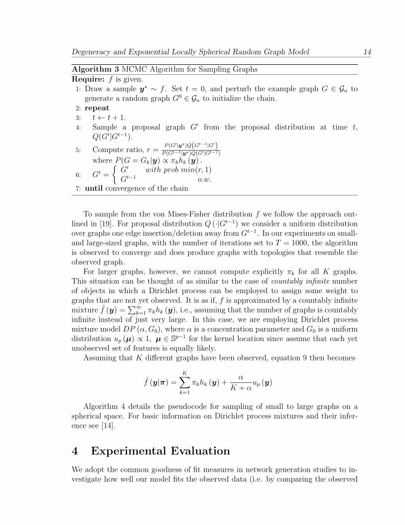
Algorithm 3 MCMC Algorithm for Sampling Graphs

Require: f is given.1: Draw a sample y? ∼ f . Set t = 0, and perturb the example graph G ∈ Gn to

generate a random graph G0 ∈ Gn to initialize the chain.2: repeat3: t← t+ 1.4: Sample a proposal graph G′ from the proposal distribution at time t,

Q(G′|Gt−1).

5: Compute ratio, r =P (G′|y?)Q(Gt−1|G′)P (Gt−1|y?)Q(G′|Gt−1)

where P (G = Gk|y) ∝ πkhk (y) .

6: Gt =

{G′ with prob min(r, 1)Gt−1 o.w.

7: until convergence of the chain

To sample from the von Mises-Fisher distribution f we follow the approach out-lined in [19]. For proposal distribution Q (·|Gt−1) we consider a uniform distributionover graphs one edge insertion/deletion away from Gt−1. In our experiments on small-and large-sized graphs, with the number of iterations set to T = 1000, the algorithmis observed to converge and does produce graphs with topologies that resemble theobserved graph.

For larger graphs, however, we cannot compute explicitly πk for all K graphs.This situation can be thought of as similar to the case of countably infinite numberof objects in which a Dirichlet process can be employed to assign some weight tographs that are not yet observed. It is as if, f is approximated by a countably infinitemixture f (y) =

∑∞k=1 πkhk (y), i.e., assuming that the number of graphs is countably

infinite instead of just very large. In this case, we are employing Dirichlet processmixture model DP (α,G0), where α is a concentration parameter and G0 is a uniformdistribution up (µ) ∝ 1, µ ∈ Sp−1 for the kernel location since assume that each yetunobserved set of features is equally likely.

Assuming that K different graphs have been observed, equation 9 then becomes

f (y|π) =K∑k=1

πkhk (y) +α

K + αup (y)

Algorithm 4 details the pseudocode for sampling of small to large graphs on aspherical space. For basic information on Dirichlet process mixtures and their infer-ence see [14].

4 Experimental Evaluation

We adopt the common goodness of fit measures in network generation studies to in-vestigate how well our model fits the observed data (i.e. by comparing the observed


Algorithm 4 MCMC-DP Algorithm for Sampling Graphs

Require: f is given. Graphs G1, . . . , GL initially observed. Set K = L. Estimate πby minimizing (10).

1: Draw a sample y? ∼ f . Set t = 0, and perturb6 the example graph G ∈ Gn togenerate a random graph G0 ∈ Gn to initialize the chain.

2: repeat3: t← t+ 1.4: Sample a proposal graph G′ from the proposal distribution at time t,

Q(G′|Gt−1).

5: Compute ratio, r = P (G′|y?)Q(Gt−1|G′)P (Gt−1|y?)Q(G′|Gt−1)

6: where

P (G = Gk|y) ∝

{πkhk (y) k = 1, . . . , K,α

K+αup (y) G = new.

7: Set Gt =

{G′ with prob min(r, 1)Gt−1 o.w.

8: If Gt is new, then set K = K + 1, GK = Gt.

• Compute f(GK), set B = B ∪ f(GK).

• Re-compute S (B) (to generalize to new samples) and re-estimateπ1, . . . , πK .

9: until convergence of the chain

statistics with a range of the same statistics obtained from simulating many networksusing the fitted model) [9]. If the observed network is not typical of the simulatednetworks for a particular measure then the model is either degenerate or simply amisfit. We first consider the degree distribution, which is defined as the statistics:D0, D1, · · · , Dn−1, with each Di representing the number of nodes with i edges con-nected to them, divided by n. Secondly, we compute the edgewise shared partnerdistribution, which is defined as the statistics: EP0, EP1, · · · , EPn−2, with each EPirepresenting the number of edges in the graph between two nodes that share exactlyi neighbors in common, divided by the total number of edges. Thirdly, we computethe triad census distribution, which is the proportion of 3 − node sets having 0, 1, 2,or 3 edges among them. Lastly, we compute the minimum geodesic distance distribu-tion; which is the proportion of pairs of nodes whose shortest connecting path is oflength k, for k = 1, 2, · · · . Also, pairs of nodes that are not connected are classifiedas k =∞.

In all our experiments, we define each feature vector to be,

f (G) =(fedge, f2?, · · · , f(11)?, f4

)TThese features have been observed to be among the set of subgraph patterns thatcapture social interactions and network formation in real processes [4].


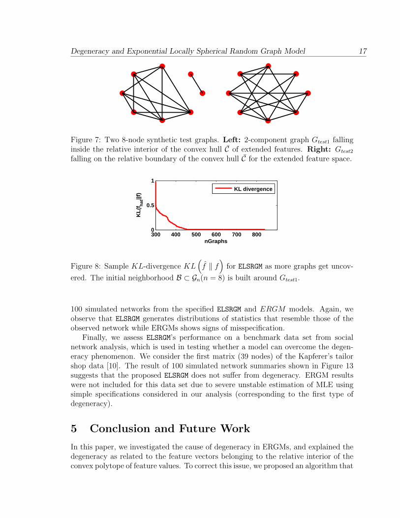
4.1 Small graphs

We first consider the experiments for Gn with n = 8 nodes. Figure 7 (left) shows a twocomponent 8-node synthetic graph, Gtest1 , while Figure 8 displays the KL-divergence

KL(f ‖ f

)computed by first observing 300 8-node graphs (graph-edit distance ≤ 3

of neighborhood around Gtest1), and allowing the MCMC-DP (Algorithm 4) to discoverand fill-in the neighborhood set B, with the baseline VMFD centered at the coor-dinates of Gtest1 . Gtest1 was chosen to test our hypothesis for the extended featurespace, that is if x? ∈ rint(C) e.g. x? = f (Gtest1) ∈ rint

(C), then the corresponding

ERGM will be degenerate in relation to the analysis of Theorem 1. Gtest2 is usedto test our second hypothesis, i.e. if x? ∈ rbd(C) then the ERGM specified by x?

is most likely to generate realistic graphs. In Figure 7 (right) we show an 8-nodesynthetic graph Gtest2 whose extended feature vector (x? = f (Gtest2) ∈ rbd

(C)).

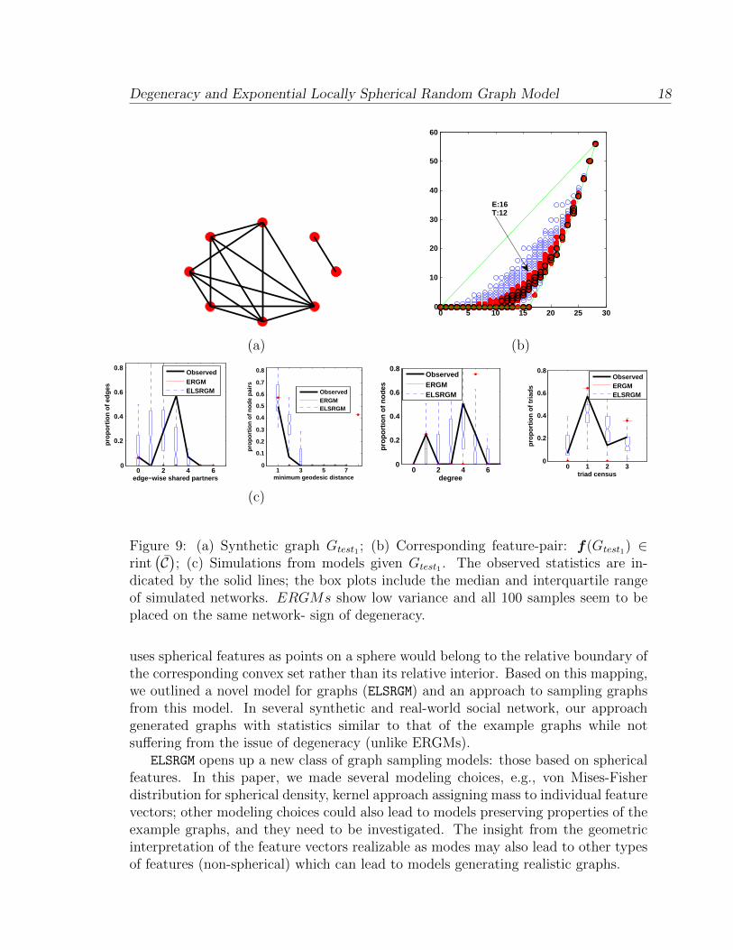
For the experimental set-up, the bandwidth for each kernel hk is treated as a userdefined parameter and is set to κhk = 400, while the DP prior parameter is set toα = 0.5. Parameters for the VMFD are set as discussed in section 3, with κ fixedat 140 to control the concentration of fVMFD. We compute the parameters for theERGM model P and simulations using the statnet package [6].

Figure 9, depicts 100 simulated summary results for f(Gtest1) ∈ rint(C). The

result obtained from our ELSRGM (in unshaded blue box plots), displays no sign ofdegeneracy while the ERGM result shows summary statistics that appear to relateto those of empty and complete graphs- a sign of degeneracy. Figure 10, showssummary statistics of simulated networks obtained for the ERGM and the ELSRGM

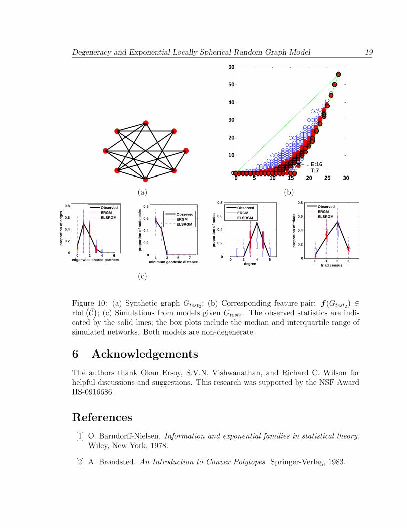
models when f(Gtest2) ∈ rbd(C). The results show no sign of degeneracy from both

the specified ERGM and the proposed ELSRGM . This confirms our second hypothesis,that is having extended feature vectors lie on the relative boundary of the convex hullenables the generation of realistic graphs from exponential family models.

4.2 Larger Graphs

For larger data sets, we first consider a undirected Dolphin social network with 62nodes [3, 11]. We apply the MCMCDP approach as outlined in Algorithm 4, by samplinggraphs via a random walk for 1000 steps starting from a random network G0 ∈ B.Figure 11 summarizes the results of 100 simulations for the Dolphin network fromthe two approaches. The proposed ELSRGM shows a relatively better performance ofcapturing the distribution of statistics of the Dolphin network. It is appears thatERGM model specified by simple statistics is incapable of generating the distributionof statistics that resembles those of the observed network. The lack of fit by an ERGMmodel in the degree distribution, geodesic distance, and shared partners distributionindicates the presence of degeneracy.

We next evaluate ELSRGM on 205-node Faux-Mesa-High social network [6, 15].We again apply the MCMC-DP algorithm by sampling graphs via a random walk for1000 steps starting from a random network G0 ∈ B. Figure 12 depicts the results of


Figure 7: Two 8-node synthetic test graphs. Left: 2-component graph Gtest1 fallinginside the relative interior of the convex hull C of extended features. Right: Gtest2

falling on the relative boundary of the convex hull C for the extended feature space.

300 400 500 600 700 8000

0.5

1

nGraphs

KL

(fh

at||f

)

KL divergence

Figure 8: Sample KL-divergence KL(f ‖ f

)for ELSRGM as more graphs get uncov-

ered. The initial neighborhood B ⊂ Gn(n = 8) is built around Gtest1.

100 simulated networks from the specified ELSRGM and ERGM models. Again, weobserve that ELSRGM generates distributions of statistics that resemble those of theobserved network while ERGMs shows signs of misspecification.

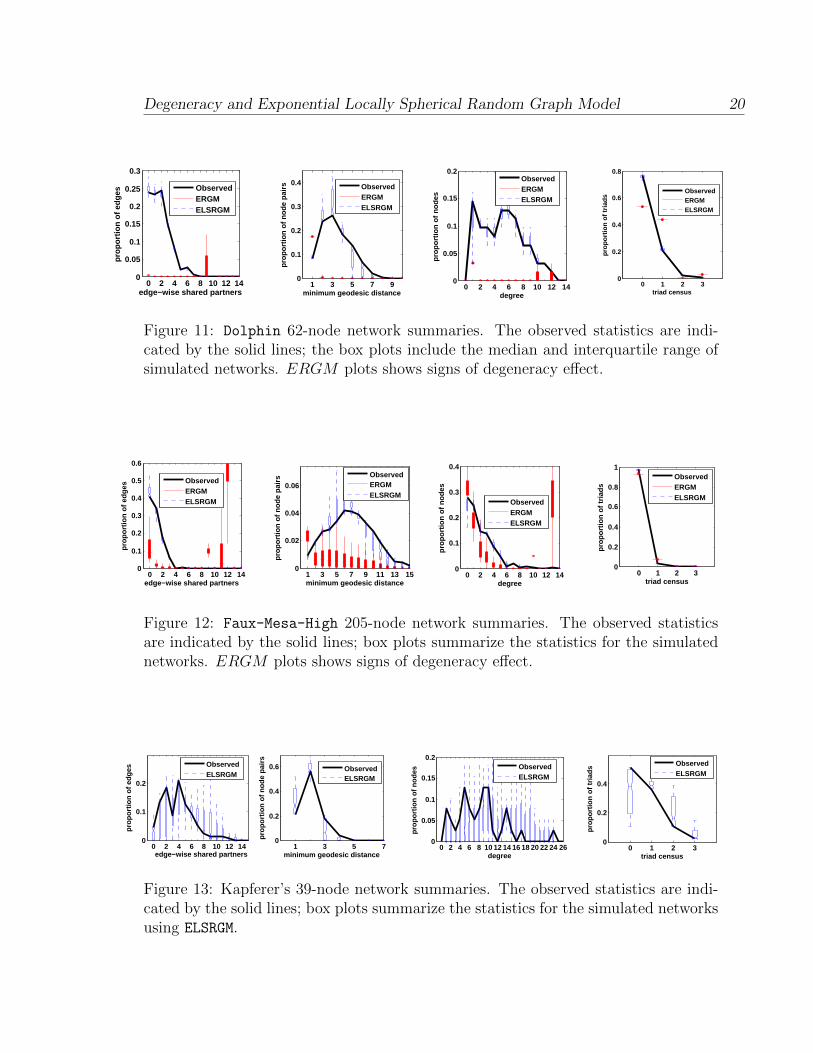
Finally, we assess ELSRGM’s performance on a benchmark data set from socialnetwork analysis, which is used in testing whether a model can overcome the degen-eracy phenomenon. We consider the first matrix (39 nodes) of the Kapferer’s tailorshop data [10]. The result of 100 simulated network summaries shown in Figure 13suggests that the proposed ELSRGM does not suffer from degeneracy. ERGM resultswere not included for this data set due to severe unstable estimation of MLE usingsimple specifications considered in our analysis (corresponding to the first type ofdegeneracy).

5 Conclusion and Future Work

In this paper, we investigated the cause of degeneracy in ERGMs, and explained thedegeneracy as related to the feature vectors belonging to the relative interior of theconvex polytope of feature values. To correct this issue, we proposed an algorithm that


(a)

0 5 10 15 20 25 300

10

20

30

40

50

60

E:16T:12

(b)

0 2 4 60

0.2

0.4

0.6

0.8

edge−wise shared partners

prop

ortio

n of

edg

es

ObservedERGMELSRGM

1 3 5 70

0.1

0.2

0.3

0.4

0.5

0.6

0.7

0.8

minimum geodesic distance

pro

po

rtio

n o

f n

od

e p

airs

ObservedERGMELSRGM

0 2 4 60

0.2

0.4

0.6

0.8

degree

pro

po

rtio

n o

f n

od

es

ObservedERGMELSRGM

0 1 2 30

0.2

0.4

0.6

0.8

triad census

pro

po

rtio

n o

f tr

iad

s

ObservedERGMELSRGM

(c)

Figure 9: (a) Synthetic graph Gtest1 ; (b) Corresponding feature-pair: f(Gtest1) ∈rint

(C); (c) Simulations from models given Gtest1 . The observed statistics are in-

dicated by the solid lines; the box plots include the median and interquartile rangeof simulated networks. ERGMs show low variance and all 100 samples seem to beplaced on the same network- sign of degeneracy.

uses spherical features as points on a sphere would belong to the relative boundary ofthe corresponding convex set rather than its relative interior. Based on this mapping,we outlined a novel model for graphs (ELSRGM) and an approach to sampling graphsfrom this model. In several synthetic and real-world social network, our approachgenerated graphs with statistics similar to that of the example graphs while notsuffering from the issue of degeneracy (unlike ERGMs).

ELSRGM opens up a new class of graph sampling models: those based on sphericalfeatures. In this paper, we made several modeling choices, e.g., von Mises-Fisherdistribution for spherical density, kernel approach assigning mass to individual featurevectors; other modeling choices could also lead to models preserving properties of theexample graphs, and they need to be investigated. The insight from the geometricinterpretation of the feature vectors realizable as modes may also lead to other typesof features (non-spherical) which can lead to models generating realistic graphs.


(a)

0 5 10 15 20 25 300

10

20

30

40

50

60

E:16T:7

(b)

0 2 4 60

0.2

0.4

0.6

0.8


prop

ortio

n of

edg

es

ObservedERGMELSRGM

1 3 5 70

0.2

0.4

0.6

0.8


pro

po

rtio

n o

f n

od

e p

airs

ObservedERGMELSRGM

0 2 4 60

0.2

0.4

0.6

0.8

degree

pro

po

rtio

n o

f n

od

es

Observed ERGMELSRGM

0 1 2 30

0.2

0.4

0.6

0.8

triad census

pro

po

rtio

n o

f tr

iad

s

ObservedERGMELSRGM

(c)

Figure 10: (a) Synthetic graph Gtest2 ; (b) Corresponding feature-pair: f(Gtest2) ∈rbd

(C); (c) Simulations from models given Gtest2 . The observed statistics are indi-

cated by the solid lines; the box plots include the median and interquartile range ofsimulated networks. Both models are non-degenerate.

6 Acknowledgements

The authors thank Okan Ersoy, S.V.N. Vishwanathan, and Richard C. Wilson forhelpful discussions and suggestions. This research was supported by the NSF AwardIIS-0916686.

References

[1] O. Barndorff-Nielsen. Information and exponential families in statistical theory.Wiley, New York, 1978.

[2] A. Brøndsted. An Introduction to Convex Polytopes. Springer-Verlag, 1983.


0 2 4 6 8 10 12 140

0.05

0.1

0.15

0.2

0.25

0.3


prop

ortio

n of

edg

es

ObservedERGMELSRGM

1 3 5 7 90

0.1

0.2

0.3

0.4

minimum geodesic distancep

rop

ort

ion

of

no

de

pai

rs

ObservedERGMELSRGM

0 2 4 6 8 10 12 140

0.05

0.1

0.15

0.2

degree

pro

po

rtio

n o

f n

od

es

ObservedERGMELSRGM

0 1 2 30

0.2

0.4

0.6

0.8

triad census

pro

po

rtio

n o

f tr

iad

s

Observed ERGM ELSRGM

Figure 11: Dolphin 62-node network summaries. The observed statistics are indi-cated by the solid lines; the box plots include the median and interquartile range ofsimulated networks. ERGM plots shows signs of degeneracy effect.

0 2 4 6 8 10 12 140

0.1

0.2

0.3

0.4

0.5

0.6


prop

ortio

n of

edg

es

ObservedERGM ELSRGM

1 3 5 7 9 11 13 150

0.02

0.04

0.06


pro

po

rtio

n o

f n

od

e p

airs

ObservedERGMELSRGM

0 2 4 6 8 10 12 140

0.1

0.2

0.3

0.4

degree

pro

po

rtio

n o

f n

od

es

ObservedERGM ELSRGM

0 1 2 30

0.2

0.4

0.6

0.8

1

triad census

pro

po

rtio

n o

f tr

iad

s

ObservedERGMELSRGM

Figure 12: Faux-Mesa-High 205-node network summaries. The observed statisticsare indicated by the solid lines; box plots summarize the statistics for the simulatednetworks. ERGM plots shows signs of degeneracy effect.

0 2 4 6 8 10 12 140

0.1

0.2


prop

ortio

n of

edg

es

ObservedELSRGM

1 3 5 70

0.2

0.4

0.6


pro

po

rtio

n o

f n

od

e p

airs

ObservedELSRGM

0 2 4 6 8 10 12 14 16 18 20 22 24 260

0.05

0.1

0.15

0.2

degree

pro

po

rtio

n o

f n

od

es

ObservedELSRGM

0 1 2 30

0.2

0.4

triad census

pro

po

rtio

n o

f tr

iad

s

ObservedELSRGM

Figure 13: Kapferer’s 39-node network summaries. The observed statistics are indi-cated by the solid lines; box plots summarize the statistics for the simulated networksusing ELSRGM.


[3] C. L. DuBois and P. Smyth. UCI network data repository, 2008.http://networkdata.ics.uci.edu.

[4] O. Frank and D. Strauss. Markov graphs. JASA, 81(395), September 1986.

[5] M. S. Handcock. Assessing degeneracy in statistical models of social networks.Technical Report 39, Center for Statistics and the Social Sciences, University ofWashington, 2003.

[6] M. S. Handcock, D. R. Hunter, C. T. Butts, S. M. Goodreau, and M. Mor-ris. statnet: Software tools for the representation, visualization, analysis andsimulation of network data. Journal of Statistical Software, 24(3), 2008.

[7] P. W. Holland and S. Leinhardt. An exponential family of probability distri-butions for directed graphs (with discussion). Journal of American StatisticalAssociation, 76(373), 1981.

[8] D. R. Hunter and M. Handcock. Inference in curved exponential family modelsfor networks. Journal of Computational and Graphical Statistics, 15(2), 2006.

[9] D. R. Hunter, M. S. Handcock, C. T. Butts, S. M. Goodreau, and M. Morris.ergm: A package to fit, simulate and diagnose exponential-family models fornetworks. Journal of Statistical Software, 24(3), 2008.

[10] B. Kapferer. Strategy and transaction in an African factory.Manchester: Manchester University Press., 1972. available fromhttp://www.casos.cs.cmu.edu/computational tools/datasets/external/kaptail/index2.html.

[11] D. Lusseau, K. Schneider, O. J. Boisseau, P. Haase, E. Slooten, and S. M. Daw-son. The bottlenose dolphin community of Doubtful Sound features a largeproportion of long-lasting associations. Behavioral Ecology and Sociobiology, 54,2003.

[12] K. V. Mardia and P. E. Jupp. Directional Statistics. Wiley, 2000.

[13] B. D. Mckay. Practical graph isomorphism. Congressus Numerantium, 30, 1981.

[14] R. M. Neal. Markov chain sampling methods for Dirichlet process mixture mod-els. Journal of Computational and Graphical Staitistics, 9(2):249–265, June 2000.

[15] M. D. Resnick and coauthors. Protecting adolescents from harm. findings fromthe national longitudinal study on adolescent health. Journal of American Med-ical Association, 278(8), 1997.

[16] A. Rinaldo, S. E. Fienberg, and Y. Zhou. On the geometry of discrete exponen-tial families with application to exponential random graph models. ElectronicJournal of Statistics, 3:446–484, 2009.


[17] S. Wasserman and P. Pattison. Logit models and logistic regression for socialnetworks: An introduction to Markov graphs and p? model. Psychometrii, 61(3),September 1996.

[18] R. C. Wilson, E. R. Hancock, E. Pekalska, and R. P. W. Duin. Spherical em-beddings for non-Euclidean dissimilarities. In CVPR-10, pages 1903–1910, June2010.

[19] A. T. Wood. Simulation of the von Mises-Fisher distribution. Communicationsin Statistics - Simulation and Computation, 23(1), 1994.


Figure 14: left: Faux-Mesa-High 205-node original network. right: ELSRGM generatednetwork.

Generating Similar Graphs From Spherical Features

Documents

Transcript of Generating Similar Graphs From Spherical Features