arX

iv:0

709.

0891

v2 [

gr-q

c] 4

Mar

200

8

Spherical symmetry in f(R)-gravity

S. Capozziello∗⋄, A. Stabile†, A. Troisi‡⋄⋄ Dipartimento di Scienze Fisiche and INFN,

Sez. di Napoli, Universita di Napoli ”Federico II”,Compl. Univ. di Monte S. Angelo,

Edificio G, Via Cinthia, I-80126 - Napoli, Italy and Dipartimento di Fisica ”E. R. Caianiello”,

Universita’ degli Studi di Salerno,Via S. Allende, I-84081 Baronissi (SA), Italy.

Spherical symmetry in f(R) gravity is discussed in details considering also the relations withthe weak field limit. Exact solutions are obtained for constant Ricci curvature scalar and for Ricciscalar depending on the radial coordinate. In particular, we discuss how to obtain results whichcan be consistently compared with General Relativity giving the well known post-Newtonian andpost-Minkowskian limits. Furthermore, we implement a perturbation approach to obtain solutionsup to the first order starting from spherically symmetric backgrounds. Exact solutions are given forseveral classes of f(R) theories in both R = constant and R = R(r).

PACS numbers: 04.50.+h; 04.25.Nx; 04.40.Nr

I. INTRODUCTION

The recent advent of new cosmological precision tests, capable of probing physics at very large redshifts, has changedthe modern view of cosmos ruling out the Cosmological Standard Model based on General Relativity (GR), radiationand baryonic matter. Beside the introduction of dark matter, needed to fit the astrophysical dynamics at galacticand cluster scales (i.e. to explain clustered structures), a new ingredient is requested in order to explain the observedaccelerated behavior of the Hubble flow: the dark energy.

In particular, the luminosity distance of Ia Type Supernovae [1], the Large Scale Structure [2] and the anisotropyof Cosmic Microwave Background [3] suggest that the widely accepted Cosmological Concordance Model (ΛCDM) isa spatially flat Universe, dominated by cold dark matter (CDM (∼ 0.25 ÷ 0.3%) which should explain the clusteredstructures) and dark energy (Λ ∼ 0.65÷ 0.7%), in the form of an “effective” cosmological constant, giving rise to theaccelerated behavior.

Although the cosmological constant [4, 5, 6] remains the most relevant candidate to interpret the accelerated behav-ior, several proposals have been suggested in the last few years: quintessence models, where the cosmic accelerationis generated by means of a scalar field, in a way similar to the early time inflation, acting at large scales and recentepochs [7]; models based on exotic fluids like the Chaplygin-gas [8], or non-perfect fluids [9]); phantom fields, basedon scalar fields with anomalous signature in the kinetic term [10], higher dimensional scenarios (braneworld) [11].Actually, all of these models, are based on the peculiar characteristic of introducing new sources into the cosmologicaldynamics, while it would be preferable to develop scenarios consistent with observations without invoking furtherparameters or components non-testable (up to now) at a fundamental level.

The resort to modified gravity theories, which extend in some way the GR, allows to pursue this different approach(no further unknown sources) giving rise to suitable cosmological models where a late time accelerated expansionnaturally arises.

The idea that the Einstein gravity should be extended or corrected at large scales (infrared limit) or at highenergies (ultraviolet limit) is suggested by several theoretical and observational issues. Quantum field theories incurved spacetimes, as well as the low energy limit of string theory, both imply semi - classical effective Lagrangianscontaining higher-order curvature invariants or scalar-tensor terms. In addition, GR has been tested only at solarsystem scales while it shows several shortcomings if checked at higher energies or larger scales.

Of course modifying the gravitational action asks for several fundamental challenges. These models can exhibitinstabilities [13] or ghost - like behaviors [14], while, on the other side, they should be matched with the low energylimit observations and experiments (solar system tests, PPN limit). Despite of all these issues, in the last years,

∗ e -mail address: capozziello@na.infn.it† e - mail address: stabile@sa.infn.it‡ e -mail address: antrois@gmail.com

2

several interesting results have been achieved in the framework of the so called f(R)- gravity at cosmological, galacticand solar system scales.

For example, models based on generic functions of the Ricci scalar R show cosmological solution with late timeaccelerating dynamics [16], in addition, it has been shown that some of them could agree with CMBR observationalprescriptions [17], nevertheless this matter is still argument of debate [18]. For a review of the models and theircosmological applications see, e.g.,[19, 20].

Moreover, considering f(R)-gravity in the low energy limit, it is possible to obtain corrected gravitational potentialscapable of explaining the flat rotation curves of spiral galaxies without considering huge amounts of dark matter[21, 22, 23, 24] and, furthermore, this seems the only self-consistent way to reproduce the universal rotation curve ofspiral galaxies [25]. On the other hand, several anomalies in solar system experiments could be framed and addressedin this picture [26].

In the last few years, several authors have dealt with this matter considering the Parameterized Post Newtonian(PPN) limit [27]. On the other hand, the investigation of spherically symmetric solutions for such kind of models hasbeen developed in several papers [28, 30, 31, 32]. Such an analysis deserves particular attention since it can allowto draw interesting conclusions on the effective modification of the gravitational potential induced by higher ordergravity at low energies and, in addition, it could shed new light on the PPN limit of such theories. However, in severalrecent papers, it has been shown that several classes of f(R) models fairly evade the Solar System constraints andagree with the limits of PPN-parameters, in particular with γ ∼ 1 probed by experiments [35, 36, 37, 38, 39]. This isnot the argument of the present paper, however it is important to stress that the spherical symmetry and the weakfiled limit have to be carefully considered in order to find out physically viable models.

In this paper, we are going to analyze, in a general way and without specifying a priori the form of the Lagrangian,the relation between the spherical symmetry and the weak field limit of f(R) gravity. Our aim is to develop asystematic approach considering the theoretical prescriptions to obtain a correct weak field limit in order to pointout the analogies and the differences with respect to GR. A fundamental issue is to recover the asymptotically flatsolution in absence of gravity and the well-known results related to the specific case f(R) = R, i.e. GR. Only in thissituation a correct comparison between GR and any extended gravity theory is possible from an experimental anda theoretical viewpoint. For example, as already shown in [34] and discussed in [40], the Birkhoff theorem is not ageneral result for fourth-order models also if it holds for several interesting classes of these theories as discussed, forexample, in [32, 41, 42].

The layout of the paper is the following. Sec.II is devoted to some general remarks on spherical symmetry in f(R)gravity. In particular, we derive the field equations in such a symmetry. In Sec.III, the expression of the Ricci scalarand the general form of metric components are derived in spherical symmetry discussing how recovering the correctMinkowski flat limit. Sec.IV is devoted to the discussion of spherically symmetric background solutions with constantscalar curvature considering, in particular Schwarzschild-like and Schwarzschild-de Sitter-like solutions with constantcurvature. Some remarkable f(R) models are worked out as example. In Sec. V, we discuss the cases in which thespherical symmetry is present also for the Ricci scalar depending on the radial coordinate r. This is an interestingsituation, not present in GR. In fact, as it is well known, in the Einstein theory, the Birkhoff theorem states thata spherically symmetric solution is always stationary and static [44] and the Ricci scalar is constant. In f(R) thesituation is more general and then the Ricci scalar, in principle, can evolve with radial and time coordinates. Sec.VIis devoted to the study of a perturbation approach starting from a spherically symmetric background considering thegeneral case in which the Ricci scalar is R = R(r). The motivation is due to the fact that, in GR, the Schwarzschildsolution and the weak field limit coincide under suitable conditions. This could be a good test bed to constructa well-posed weak field limit for any extended theory of gravity. Finally, we work out some f(R)-models findingspherically-symmetric solutions by the perturbation approach. Conclusions are drawn in Sec.VII.

II. SPHERICAL SYMMETRY

Let us consider an analytic function f(R) of the Ricci scalar R. The variational principle for this action is:

δ

∫

d4x√−g

[

f(R) + XLm

]

= 0 (1)

where X =16πG

c4, Lm is the standard matter Lagrangian and g is the determinant of the metric. By varying with

3

respect to the metric, we obtain the field equations 1

f ′(R)Rµν − 1

2f(R)gµν − f ′(R);µν + gµνf ′(R) =

X2

Tµν , (2)

where the trace equation read

3f ′(R) + f ′(R)R − 2f(R) =X2

T , (3)

and Tµν =−2√−g

δ(√−gLm)

δgµνis the energy momentum tensor of standard matter, T = T σ

σ is the related trace and

f ′(R) = df(R)dR

. Eqs.(2) can be rewritten in an Einstein-like form recasting the higher than second order contributionsunder the form of an effective stress - energy tensor of geometrical origin:

Gµν = Rµν − 1

2Rgµν = T (curv)

µν + T (m)µν . (4)

The effective curvature stress - energy tensor is [15] :

T (curv)µν =

1

f ′(R)gµν [f(R) − Rf ′(R)] + f ′(R);ρσ (gµρgνσ − gρσgµν) . (5)

The matter term enters Eqs.(4) through the modified stress - energy tensor :

T (m)µν =

XTµν

2f ′(R), (6)

where there is a non-minimal coupling between matter and geometric degrees of freedom. For the purposes of thispaper, we will refer to the field equations in the form (2) which reveal to be more useful for the following considerations.

The most general spherically symmetric metric can be written as follows :

ds2 = m1(t′, r′)dt′2 + m2(t

′, r′)dr′2 + m3(t′, r′)dt′dr′ + m4(t

′, r′)dΩ , (7)

where mi are functions of the radius r′ and of the time t′ (see also [32]). In GR, due to the freedom in the framechoice, we can consider a coordinate transformation t = U1(t

′, r′) , r = U2(t′, r′) which maps the metric (7) in a new

one where the off - diagonal term m3(t′, r′)dt′dr′ vanishes and m4(t

′, r′) = −r2, that is2 :

ds2 = A(t, r)dt2 − B(t, r)dr2 − r2dΩ . (8)

This expression can be considered without loss of generality as the most general definition of a spherically symmetricmetric compatible with a pseudo -Riemannian manifold without torsion. Actually, by inserting this metric into thefield equations (2) and (3), one obtains :

f ′(R)Rµν − 1

2f(R)gµν + Hµν =

X2

Tµν , (9)

gστHστ = f ′(R)R − 2f(R) + H =X2

T , (10)

1 It is possible to take into account also the Palatini approach in which the metric g and the connection Γ are considered independentvariables (see for example [45]). Here we will consider the Levi-Civita connection and will use the metric approach. See [19, 46] for adetailed comparison between the two pictures.

2 This condition allows to obtain the standard definition of the circumference with radius r.

4

where the two quantities Hµν and H read :

Hµν = −f ′′(R)

R,µν − ΓtµνR,t − Γr

µνR,r − gµν

[(

gtt,t + gtt ln

√−g,t

)

R,t +

(

grr,r + grr ln

√−g,r

)

R,r +

+gttR,tt + grrR,rr

]

− f ′′′(R)

[

R,µR,ν − gµν

(

gttR,t2 + grrR,r

2

)]

(11)

H = gστHστ = 3f ′′(R)

[(

gtt,t + gtt ln

√−g,t

)

R,t +

(

grr,r + grr ln

√−g,r

)

R,r + gttR,tt + grrR,rr

]

+

+3f ′′′(R)

[

gttR,t2 + grrR,r

2

]

, (12)

where Γαµν are the standard Christoffel’s symbols related to the metric gµν . These equations show the interesting

feature that the derivatives with respect to R of f(R) are very well distinct with respect to the time and spatialderivatives of R. This peculiarity will allow to better understand the dynamical behavior of solutions, as we shall seebelow.

III. THE RICCI CURVATURE SCALAR IN SPHERICAL SYMMETRY

As standard, the Ricci scalar can be written as

R = gµνRµν = gµν[

Γαµν,α − Γα

µα,ν + ΓβαβΓα

µν − ΓαβµΓβ

να

]

, (13)

where Γαµν is the Christoffel symbols defined as

Γαµν =

1

2gασ (gµσ,ν + gνσ,µ − gµν,σ) . (14)

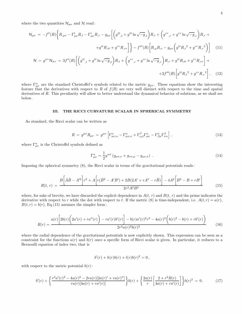
Imposing the spherical symmetry (8), the Ricci scalar in terms of the gravitational potentials reads :

R(t, r) =

B

[

AB − A′2

]

r2 + A

[

r(B2 − A′B′) + 2B(2A′ + rA′′ − rB)

]

− 4A2

[

B2 − B + rB′

]

2r2A2B2(15)

where, for sake of brevity, we have discarded the explicit dependence in A(t, r) and B(t, r) and the prime indicates thederivative with respect to r while the dot with respect to t. If the metric (8) is time-independent, i.e. A(t, r) = a(r),B(t, r) = b(r), Eq.(15) assumes the simpler form :

R(r) =

a(r)

[

2b(r)

(

2a′(r) + ra′′(r)

)

− ra′(r)b′(r)

]

− b(r)a′(r)2r2 − 4a(r)2(

b(r)2 − b(r) + rb′(r)

)

2r2a(r)2b(r)2(16)

where the radial dependence of the gravitational potentials is now explicitly shown. This expression can be seen as aconstraint for the functions a(r) and b(r) once a specific form of Ricci scalar is given. In particular, it reduces to aBernoulli equation of index two, that is

b′(r) + h(r)b(r) + l(r)b(r)2 = 0 ,

with respect to the metric potential b(r) :

b′(r) +

r2a′(r)2 − 4a(r)2 − 2ra(r)[2a(r)′ + ra(r)′′]

ra(r)[4a(r) + ra′(r)]

b(r) +

2a(r)

r

[

2 + r2R(r)

4a(r) + ra′(r)

]

b(r)2 = 0 . (17)

5

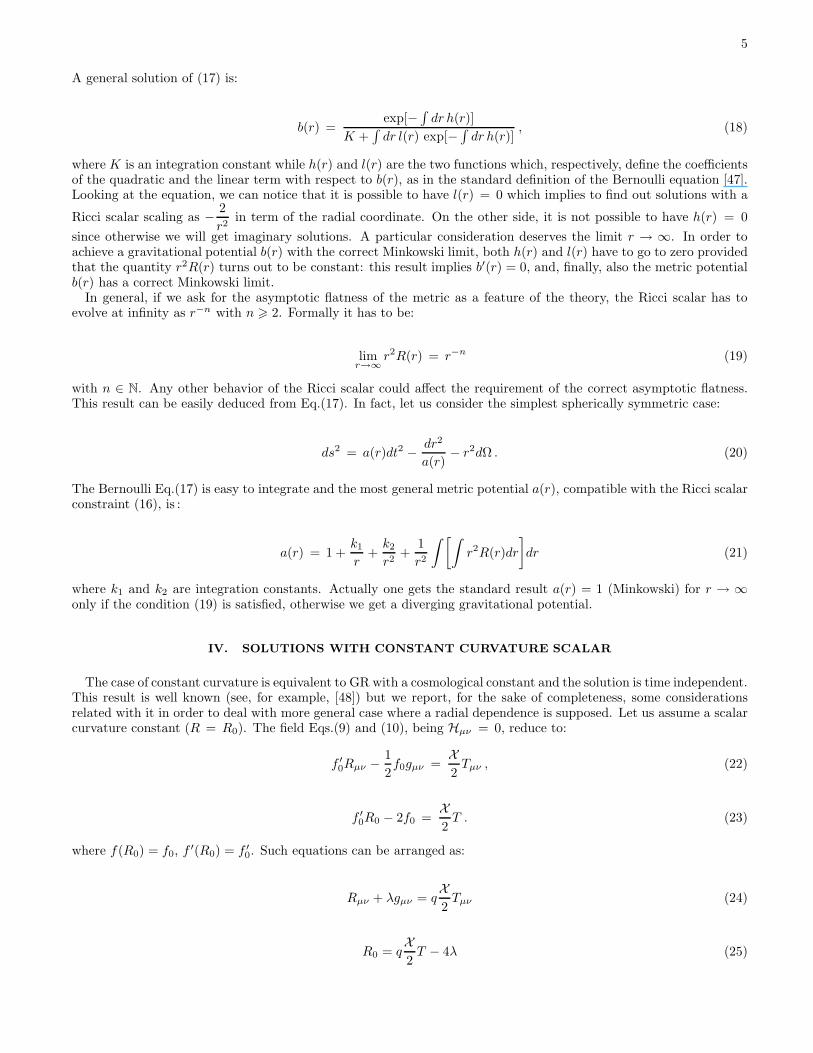
A general solution of (17) is:

b(r) =exp[−

∫

dr h(r)]

K +∫

dr l(r) exp[−∫

dr h(r)], (18)

where K is an integration constant while h(r) and l(r) are the two functions which, respectively, define the coefficientsof the quadratic and the linear term with respect to b(r), as in the standard definition of the Bernoulli equation [47].Looking at the equation, we can notice that it is possible to have l(r) = 0 which implies to find out solutions with a

Ricci scalar scaling as − 2

r2in term of the radial coordinate. On the other side, it is not possible to have h(r) = 0

since otherwise we will get imaginary solutions. A particular consideration deserves the limit r → ∞. In order toachieve a gravitational potential b(r) with the correct Minkowski limit, both h(r) and l(r) have to go to zero providedthat the quantity r2R(r) turns out to be constant: this result implies b′(r) = 0, and, finally, also the metric potentialb(r) has a correct Minkowski limit.

In general, if we ask for the asymptotic flatness of the metric as a feature of the theory, the Ricci scalar has toevolve at infinity as r−n with n > 2. Formally it has to be:

limr→∞

r2R(r) = r−n (19)

with n ∈ N. Any other behavior of the Ricci scalar could affect the requirement of the correct asymptotic flatness.This result can be easily deduced from Eq.(17). In fact, let us consider the simplest spherically symmetric case:

ds2 = a(r)dt2 − dr2

a(r)− r2dΩ . (20)

The Bernoulli Eq.(17) is easy to integrate and the most general metric potential a(r), compatible with the Ricci scalarconstraint (16), is :

a(r) = 1 +k1

r+

k2

r2+

1

r2

∫[∫

r2R(r)dr

]

dr (21)

where k1 and k2 are integration constants. Actually one gets the standard result a(r) = 1 (Minkowski) for r → ∞only if the condition (19) is satisfied, otherwise we get a diverging gravitational potential.

IV. SOLUTIONS WITH CONSTANT CURVATURE SCALAR

The case of constant curvature is equivalent to GR with a cosmological constant and the solution is time independent.This result is well known (see, for example, [48]) but we report, for the sake of completeness, some considerationsrelated with it in order to deal with more general case where a radial dependence is supposed. Let us assume a scalarcurvature constant (R = R0). The field Eqs.(9) and (10), being Hµν = 0, reduce to:

f ′0Rµν − 1

2f0gµν =

X2

Tµν , (22)

f ′0R0 − 2f0 =

X2

T . (23)

where f(R0) = f0, f ′(R0) = f ′0. Such equations can be arranged as:

Rµν + λgµν = qX2

Tµν (24)

R0 = qX2

T − 4λ (25)

6

where λ = − f0

2f ′0

and q−1 = f ′0. As standard, the stress-energy tensor of perfect-fluid matter is

Tµν = (ρ + p)uµuν − pgµν ; (26)

where ρ is the energy density, p is the pressure and uµ = dxµ/ds is the 4-velocity. A general solution of the above setof equations is achieved for p = −ρ and reads :

ds2 =

(

1 +k1

r+

qXρ − 2λ

6r2

)

dt2 − dr2

1 + k1

r+ qXρ−2λ

6 r2− r2dΩ . (27)

This result means that any f(R) - theory in the case of constant curvature scalar (R = R0) exhibits solutions withcosmological constant - like behavior (de Sitter). This is one of the reason why the dark energy issue can be addressedusing these theory [15, 16]. This fact is well known using the FRW metric [48]. As another remark we have to saythat this solution cannot describe stellar structures since this kind of equation of state does not work for stars so itcould be interesting only in cosmological contexts.

If f(R) is analytic, it is:

f(R) = Λ + Ψ0R + Ψ(R) . (28)

where Ψ0 is a coupling constant, Λ plays the role of the cosmological constant and Ψ(R) is a generic analytic functionof R satisfying the condition

limR→0

R−2Ψ(R) = Ψ1 (29)

where Ψ1 is a constant. If we neglect the cosmological constant Λ and Ψ0 is set to zero, we obtain a new class oftheories which, in the limit R → 0, does not reproduce GR (from Eq.(29), we have limR→0 f(R) ∼ R2). In such a caseanalyzing the whole set of Eqs.(22) and (23), one can observe that both zero and constant 6= 0 curvature solutions arepossible. In particular, if R = R0 = 0 field equations are solved for every form of gravitational potentials enteringthe spherically symmetric background, provided that the Bernoulli equation (17), relating these functions, is fulfilledfor the particular case R(r) = 0. The solutions are thus defined by the relation

b(r) =exp[−

∫

dr h(r)]

K + 4∫ dr a(r) exp[−

R

dr h(r)]r[a(r)+ra′(r)]

, (30)

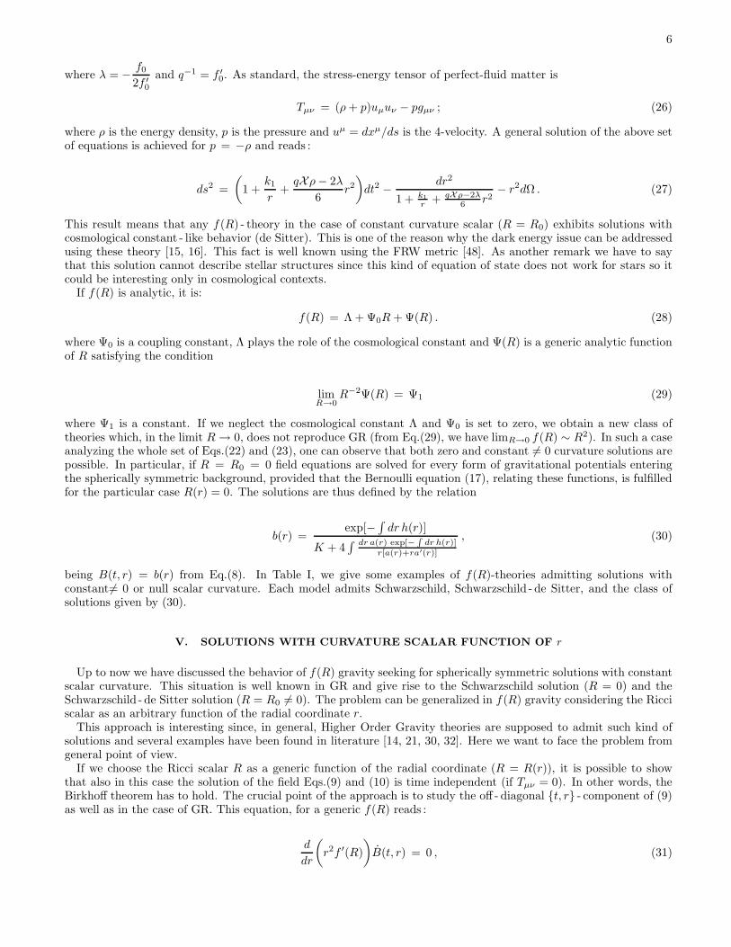
being B(t, r) = b(r) from Eq.(8). In Table I, we give some examples of f(R)-theories admitting solutions withconstant6= 0 or null scalar curvature. Each model admits Schwarzschild, Schwarzschild - de Sitter, and the class ofsolutions given by (30).

V. SOLUTIONS WITH CURVATURE SCALAR FUNCTION OF r

Up to now we have discussed the behavior of f(R) gravity seeking for spherically symmetric solutions with constantscalar curvature. This situation is well known in GR and give rise to the Schwarzschild solution (R = 0) and theSchwarzschild - de Sitter solution (R = R0 6= 0). The problem can be generalized in f(R) gravity considering the Ricciscalar as an arbitrary function of the radial coordinate r.

This approach is interesting since, in general, Higher Order Gravity theories are supposed to admit such kind ofsolutions and several examples have been found in literature [14, 21, 30, 32]. Here we want to face the problem fromgeneral point of view.

If we choose the Ricci scalar R as a generic function of the radial coordinate (R = R(r)), it is possible to showthat also in this case the solution of the field Eqs.(9) and (10) is time independent (if Tµν = 0). In other words, theBirkhoff theorem has to hold. The crucial point of the approach is to study the off - diagonal t, r - component of (9)as well as in the case of GR. This equation, for a generic f(R) reads :

d

dr

(

r2f ′(R)

)

B(t, r) = 0 , (31)

7

f(R) - theory: Field equations:

R −→ Rµν = 0, with R = 0

ξ1R + ξ2Rn −→

8

>

>

>

>

>

>

<

>

>

>

>

>

>

:

Rµν = 0 with R = 0, ξ1 6= 0

Rµν + λgµν = 0 with R =

»

ξ1(n−2)ξ2

– 1n−1

, ξ1 6= 0, n 6= 2

0 = 0 with R = 0, ξ1 = 0

Rµν + λgµν = 0 with R = R0, ξ1 = 0, n = 2

ξ1R + ξ2R−m −→ Rµν + λgµν = 0 with R =

»

−(m+2)ξ2

ξ1

– 1m+1

ξ1R + ξ2Rn + ξ3R

−m −→ Rµν + λgµν = 0, with R = R0 so that ξ1Rm+10 + (2 − n)ξ2R

n+m0 + (m + 2)ξ3 = 0

Rξ1+R

−→

(

Rµν = 0 with R = 0

Rµν + λgµν = 0 with R = − ξ12

1ξ1+R

−→ Rµν + λgµν = 0, with R = − 2ξ13

TABLE I: Emamples of f(R)-models admitting constant and zero scalar curvature solutions. In the right hand side, the fieldequations are given for each model. The power n, m are natural numbers while ξi are generic real constants.

and two possibilities are in order. Firstly, we can choose B(t, r) 6= 0. This choice implies that f ′(R) ∼ 1

r2. If this is

the case, the remaining field equation turn out to be not fulfilled and it can be easily recognized that the dynamicalsystem encounters a mathematical incompatibility.

The only possible solution is given by B(t, r) = 0 and then the gravitational potential has to be B(t, r) = b(r).Considering also the θ, θ - equation one can determine that the gravitational potential A(t, r) can be factorized withrespect to the time, so that we get solutions which can be recast in the stationary spherically symmetric form after asuitable coordinate transformation.

As a matter of fact, even the more general radial dependent case admit time - independent solutions. From thetrace equation and the θ, θ - component, we deduce a relation which links A(t, r) = a(r) and B(t, r) = b(r) :

a(r) =b(r)e

23

R (Rf′−2f)b(r)

R′f′′ dr

r4R′2f ′′2, (32)

(with f ′′ 6= 0) and one which relates b(r) and f(R) (see also [30] for a similar result) :

b(r) =6[f ′(rR′f ′′)′ − rR′2f ′′2]

rf(rR′f ′′ − 4f ′) + 2f ′(rR(f ′ − rR′f ′′) − 3R′f ′′). (33)

As above, three further equations has to be satisfied to completely solve the system (respectively the t, t andr, r components of the field equations and the Ricci scalar constraint) while the only unknown functions are f(R)and the Ricci scalar R(r).

If we now consider a fourth order model of the form f(R) = R+Φ(R), with Φ(R) ≪ R we are capable of satisfyingthe whole set of equations up to third order in Φ. In particular, we can solve the whole set of equations: the relations(32) and (33) will give the general solution depending only on the forms of Φ(R) and R = R(r), that is:

8

a(r) =b(r)e

−2

3

∫

[R + (2Φ − RΦ′)]b(r)

R′Φ′′dr

r4R′2Φ′′2(34)

b(r) = −3(rR′Φ′′),r

rR. (35)

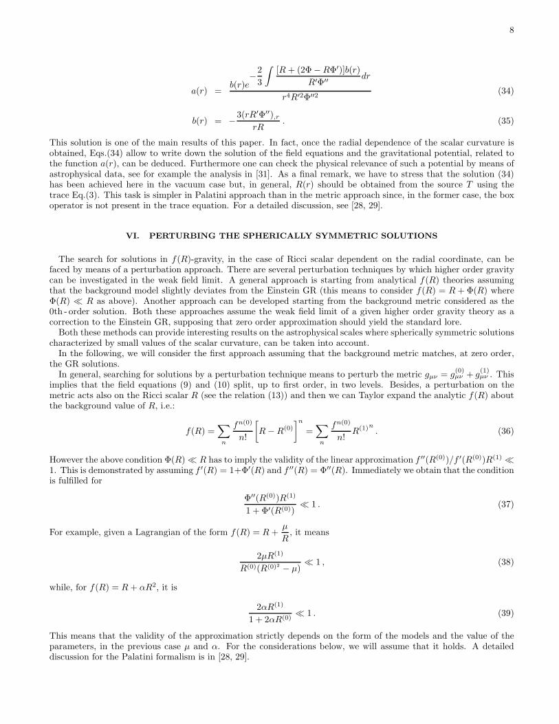
This solution is one of the main results of this paper. In fact, once the radial dependence of the scalar curvature isobtained, Eqs.(34) allow to write down the solution of the field equations and the gravitational potential, related tothe function a(r), can be deduced. Furthermore one can check the physical relevance of such a potential by means ofastrophysical data, see for example the analysis in [31]. As a final remark, we have to stress that the solution (34)has been achieved here in the vacuum case but, in general, R(r) should be obtained from the source T using thetrace Eq.(3). This task is simpler in Palatini approach than in the metric approach since, in the former case, the boxoperator is not present in the trace equation. For a detailed discussion, see [28, 29].

VI. PERTURBING THE SPHERICALLY SYMMETRIC SOLUTIONS

The search for solutions in f(R)-gravity, in the case of Ricci scalar dependent on the radial coordinate, can befaced by means of a perturbation approach. There are several perturbation techniques by which higher order gravitycan be investigated in the weak field limit. A general approach is starting from analytical f(R) theories assumingthat the background model slightly deviates from the Einstein GR (this means to consider f(R) = R + Φ(R) whereΦ(R) ≪ R as above). Another approach can be developed starting from the background metric considered as the0th - order solution. Both these approaches assume the weak field limit of a given higher order gravity theory as acorrection to the Einstein GR, supposing that zero order approximation should yield the standard lore.

Both these methods can provide interesting results on the astrophysical scales where spherically symmetric solutionscharacterized by small values of the scalar curvature, can be taken into account.

In the following, we will consider the first approach assuming that the background metric matches, at zero order,the GR solutions.

In general, searching for solutions by a perturbation technique means to perturb the metric gµν = g(0)µν + g

(1)µν . This

implies that the field equations (9) and (10) split, up to first order, in two levels. Besides, a perturbation on themetric acts also on the Ricci scalar R (see the relation (13)) and then we can Taylor expand the analytic f(R) aboutthe background value of R, i.e.:

f(R) =∑

n

fn(0)

n!

[

R − R(0)

]n

=∑

n

fn(0)

n!R(1)n

. (36)

However the above condition Φ(R) ≪ R has to imply the validity of the linear approximation f ′′(R(0))/f ′(R(0))R(1) ≪1. This is demonstrated by assuming f ′(R) = 1+Φ′(R) and f ′′(R) = Φ′′(R). Immediately we obtain that the conditionis fulfilled for

Φ′′(R(0))R(1)

1 + Φ′(R(0))≪ 1 . (37)

For example, given a Lagrangian of the form f(R) = R +µ

R, it means

2µR(1)

R(0)(R(0)2 − µ)≪ 1 , (38)

while, for f(R) = R + αR2, it is

2αR(1)

1 + 2αR(0)≪ 1 . (39)

This means that the validity of the approximation strictly depends on the form of the models and the value of theparameters, in the previous case µ and α. For the considerations below, we will assume that it holds. A detaileddiscussion for the Palatini formalism is in [28, 29].

9

The zero order field equations read :

f ′(0)R(0)µν − 1

2g(0)

µν f (0) + H(0)µν =

X2

T (0)µν (40)

where

H(0)µν = −f ′′(0)

R(0),µν − Γ(0)ρ

µνR(0),ρ − g(0)

µν

(

g(0)ρσ,ρR

(0),σ + g(0)ρσR(0)

,ρσ + g(0)ρσ ln√−g,ρR

(0),σ

)

+

−f ′′′(0)

R(0),µ R(0)

,ν − g(0)µν g(0)ρσR(0)

,ρ R(0),σ

. (41)

At first order one has :

f ′(0)

R(1)µν − 1

2g(0)

µν R(1)

+ f ′′(0)R(1)R(0)µν − 1

2f (0)g(1)

µν + H(1)µν =

X2

T (1)µν (42)

with

H(1)µν = −f ′′(0)

R(1),µν − Γ(0)ρ

µνR(1),ρ − Γ(1)ρ

µνR(0),ρ − g(0)

µν

[

g(0)ρσ,ρR

(1),σ + g(1)ρσ

,ρR(0),σ + g(0)ρσR(1)

,ρσ +

+g(1)ρσR(0),ρσ + g(0)ρσ

(

ln√−g

(0),ρ R(1)

,σ + ln√−g

(1),ρ R(0)

,σ

)

+g(1)ρσ ln√−g

(0),ρ R(0)

,σ

]

− g(1)µν

(

g(0)ρσ,ρR

(0),σ +

+g(0)ρσR(0),ρσ + g(0)ρσ ln

√−g

(0),ρ R(0)

,σ

)

− f ′′′(0)

R(0),µ R(1)

,ν + R(1),µ R(0)

,ν − g(0)µν g(0)ρσ

(

R(0),ρ R(1)

,σ + R(1),ρ R(0)

,σ

)

+

−g(0)µν g(1)ρσR(0)

,ρ R(0),σ − g(1)

µν g(0)ρσR(0),ρ R(0)

,σ

− f ′′′(0)R(1)

R(0),µν − Γ(0)ρ

µνR(0),ρ − g(0)

µν

(

g(0)ρσ,ρR

(0),σ +

+g(0)ρσR(0),ρσ + g(0)ρσ ln

√−g,ρR

(0),σ

)

−f IV (0)R(1)

R(0),µ R(0)

,ν − g(0)µν g(0)ρσR(0)

,ρ R(0),σ

. (43)

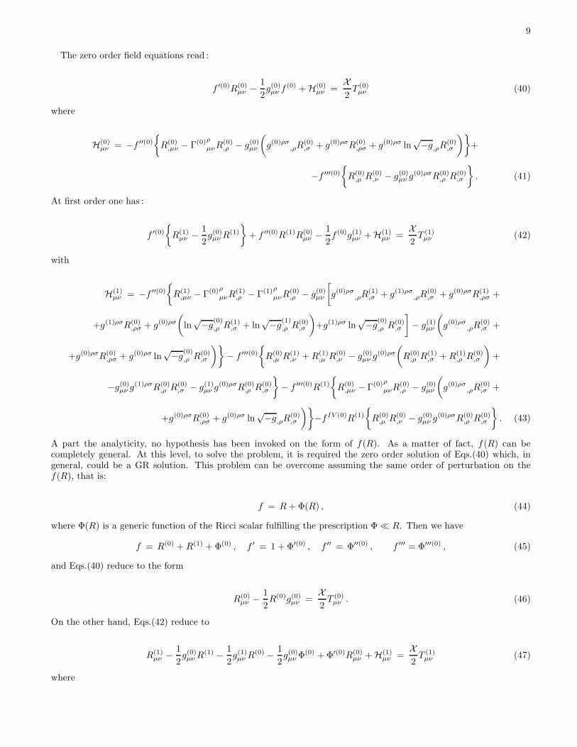
A part the analyticity, no hypothesis has been invoked on the form of f(R). As a matter of fact, f(R) can becompletely general. At this level, to solve the problem, it is required the zero order solution of Eqs.(40) which, ingeneral, could be a GR solution. This problem can be overcome assuming the same order of perturbation on thef(R), that is:

f = R + Φ(R) , (44)

where Φ(R) is a generic function of the Ricci scalar fulfilling the prescription Φ ≪ R. Then we have

f = R(0) + R(1) + Φ(0) , f ′ = 1 + Φ′(0) , f ′′ = Φ′′(0) , f ′′′ = Φ′′′(0) , (45)

and Eqs.(40) reduce to the form

R(0)µν − 1

2R(0)g(0)

µν =X2

T (0)µν . (46)

On the other hand, Eqs.(42) reduce to

R(1)µν − 1

2g(0)

µν R(1) − 1

2g(1)

µν R(0) − 1

2g(0)

µν Φ(0) + Φ′(0)R(0)µν + H(1)

µν =X2

T (1)µν (47)

where

10

H(1)µν = −Φ′′′(0)

R(0),µ R(0)

,ν − g(0)µν g(0)rrR(0)

,r R(0),r

− Φ′′(0)

R(0),µν − Γ(0)r

µν R(0),r − g(0)

µν

(

g(0)rr

,r R(0),r +

+g(0)rrR(0),rr + g(0)rr ln

√−g(0),r R(0)

,r

)

. (48)

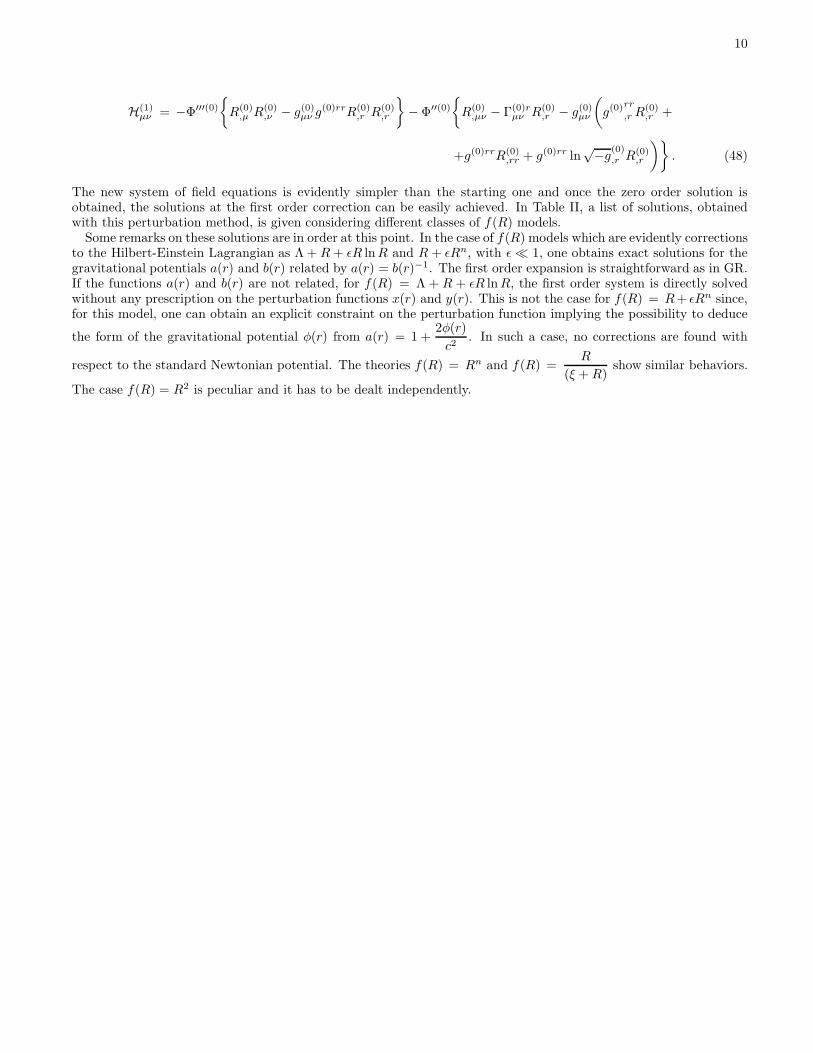
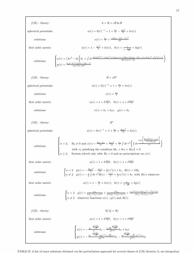
The new system of field equations is evidently simpler than the starting one and once the zero order solution isobtained, the solutions at the first order correction can be easily achieved. In Table II, a list of solutions, obtainedwith this perturbation method, is given considering different classes of f(R) models.

Some remarks on these solutions are in order at this point. In the case of f(R) models which are evidently correctionsto the Hilbert-Einstein Lagrangian as Λ + R + ǫR lnR and R + ǫRn, with ǫ ≪ 1, one obtains exact solutions for thegravitational potentials a(r) and b(r) related by a(r) = b(r)−1. The first order expansion is straightforward as in GR.If the functions a(r) and b(r) are not related, for f(R) = Λ + R + ǫR lnR, the first order system is directly solvedwithout any prescription on the perturbation functions x(r) and y(r). This is not the case for f(R) = R+ ǫRn since,for this model, one can obtain an explicit constraint on the perturbation function implying the possibility to deduce

the form of the gravitational potential φ(r) from a(r) = 1 +2φ(r)

c2. In such a case, no corrections are found with

respect to the standard Newtonian potential. The theories f(R) = Rn and f(R) =R

(ξ + R)show similar behaviors.

The case f(R) = R2 is peculiar and it has to be dealt independently.

11

f(R) - theory: Λ + R + ǫR lnR

spherical potentials: a(r) = b(r)−1 = 1 + k1r− Λr2

6+ δx(r)

solutions: x(r) = k2r

+ ǫΛ[ln(−2Λ)−1]r2

6δ

first order metric: a(r) = 1 − Λr2

6+ δx(r), b(r) = 1

1−Λr2

6

+ δy(r)

solutions:

8

>

<

>

:

x(r) = (Λr2 − 6)

k1 +R

dr 4δ(2Λ2r4−15Λr2+18)y(r)+r36rǫΛ[log(−2Λ)−1]+δ(Λr2−6)2y′(r)36rδ(Λr2−6)

ff

y(r) = k2δ−6r3ǫΛ[ln(−2Λ)−1]

rδ(r2Λ−6)2

f(R) - theory: R + ǫRn

spherical potentials: a(r) = b(r)−1 = 1 + k1r

+ δx(r)

solutions: x(r) = k2r

first order metric: a(r) = 1 + δ x(r)r

, b(r) = 1 + δ y(r)r

solutions: x(r) = k1 + k2r, y(r) = k3

f(R) - theory: Rn

spherical potentials: a(r) = b(r)−1 = 1 + k1r

+ R0r2

12+ δx(r)

solutions:

8

>

>

>

>

>

<

>

>

>

>

>

:

n = 2, R0 6= 0 and x(r) = 3k2−k33r

+ k3r2

12+ k4

r

R

dr r2

R

dr

exp

»

R0r20 ln(r−r0)

8+3R0r20

–

r5

ff

with r0 satisfying the condition 6k1 + 8r0 + R0r30 = 0

n ≥ 2, System solved only whit R0 = 0 and no prescriptions on x(r)

first order metric: a(r) = 1 + δ x(r)r

, b(r) = 1 + δ y(r)r

solutions:

(

n = 2 y(r) = −R0r3

6−

x(r)2

+ 12rx′(r) + k1, R(r) = δR0

n 6= 2 y(r) = − 12

R

dr r2R(r) − x(r)2

+ 12rx′(r) + k1 with R(r) whatever

first order metric: a(r) = 1 −rg

r+ δx(r), b(r) = 1

1− rgr

+ δy(r)

solutions:

8

<

:

n = 2 y(r) = rk13r2

g−7rgr+4r2 + r2k23(3r2

g−7rgr+4r2)+

rgr2x(r)+2(rgr3−r4)x′(r)

(3rg−4r)(rg−r)2

n 6= 2 whatever functions x(r) , y(r) and R(r)

f(R) - theory: R/(ξ + R)

first order metric: a(r) = 1 + δ x(r)r

, b(r) = 1 + δ y(r)r

solutions:

8

>

>

<

>

>

:

x(r) = − 4e− ξ1/2r√

6

ξk1 − 2

√6e

ξ1/2r√6

ξ3/2 k2 + k3r

y(r) = −2e

− ξ1/2r√6 (6ξ1/2+

√6ξ r)

3b3/2 k1 −2e

ξ1/2r√6 (

√6−ξ1/2r)

ξ3/2 k2

TABLE II: A list of exact solutions obtained via the perturbation approach for several classes of f(R) theories; ki are integration

12

VII. CONCLUSIONS

General Relativity has been consistently tested in physical situations implying, essentially, spherical symmetryand weak field limit [49]. One of the fundamental and obvious issue that any theory of gravity should satisfy isthe fact that, in absence of gravitational field or very far from a given distribution of sources, the spacetime hasto be asymptotically flat (Minkowski). Any alternative or modified gravitational theory (beside the diffeomorphisminvariance and the general covariance) should address these physical requirements to be consistently compared withGR. This is a crucial point which several times is not considered when people is constructing the weak field limit ofalternative theories of gravity.

In this paper, we have faced this problem discussing, in the most general way, what the meaning of sphericalsolutions is in f(R) theories of gravity and when the standard results of GR are recovered in the limits r → ∞ andf(R) → R. Essentially, spherical solutions can be classified, with respect to the Ricci curvature scalar R, as R = 0,R = R0 6= 0, and R = R(r), where R0 is a constant and R(r) is a function of the radial coordinate r. In these cases,the Birkhoff theorem holds; this means that stationary solutions are also static. However, as shown in the companionpaper [34], this theorem does not hold, in general, for every f(R) theory since time-dependent evolution can emergedepending on the order of perturbations.

In order to achieve exact spherical solutions, a crucial role is played by the relations existing between the metricpotentials and between them and the Ricci curvature scalar. In particular, the relations between the metric potentialsand the Ricci scalar can be used as a constraint: this gives a Bernoulli equation. Solving it, in principle, sphericallysymmetric solutions can be obtained for any analytic f(R) function, both for constant curvature scalar and forcurvature scalar depending on r.

Such spherically symmetric solutions can be used as background to test how generic f(R) theories of gravity deviatefrom GR. Particularly interesting are those theories that imply f(R) → R in the weak field limit. In such cases, theexperimental comparison is straightforward and also experimental results, evading GR constraints, can be framed ina self-consistent picture [26].

Finally, we have constructed a perturbation approach in which we search for spherically symmetric solutions atthe 0th-order and then we search for solutions at the first order. The scheme is iterative and could be, in principle,extended to any order in perturbations. The crucial request is to take into account f(R) theories which are Taylorexpandable about some value R = R0 of the curvature scalar.

A important remark is in order at this point. Considering interior and exterior solutions, the junction conditions arerelated to the integration constants of the problem and strictly depend on the source (e.g. the form of T ). We havenot considered this aspect here since we have, essentially, searched for vacuum solutions. However, such a problemhas to be carefully faced in order to deal with physically consistent solutions. For example, the Schwarzschild solutionR = 0, which is one of the exterior solutions which we have considered, always satisfies the junction conditions withphysically interesting interior metric. This is not the case for several spherically symmetric solutions which could giverise to unphysical junction conditions and not be in agreement with Newton’s law of gravitation, also asymptotically.In these cases, such solutions have to be discarded. A detailed analysis in this sense is in the paper [42] for sphericallysymmetric solutions obtained in the Palatini formalism and in [43] for the metric approach.

[1] A.G. Riess et al. Astron. J. 116, 1009 (1998); A.G. Riess et al. Astroph. Journ. 607, 665 (2004); S. Perlmutter et al.Astrophys. J 517, 565 (1999); Astron. Astrophys. 447, 31 (2006).

[2] S. Cole et al., Mon. Not. Roy. Astron. Soc. 362, 505 (2005).[3] D.N. Spergel et al. Astrophys. J. Suppl. 148, 175 (2003); D.N. Spergel et al. ApJS 170, 377 (2007).[4] T. Padmanabhan, Phys. Rept. 380, 235 (2003).[5] Peebles P.J.E., Rathra B. 2003, Rev. Mod. Phys., 75, 559.[6] E.J. Copeland, M. Sami, S. Tsujikawa, Int. J. Mod. Phys. D 15, 1753 (2006).[7] B. Rathra, P.J.E. Peebles, Phys. Rev. D 37 3406, (1988); R.R. Caldwell, R. Dave, P.J. Steinhardt, Phys. Rev. Lett. 80,

1582, (1998).[8] A.Y. Kamenshchik, U. Moshella, V. Pasquier, Phys. Lett. B 511, 265 (2001); N. Bilic, G.B. Tupper, R.D. Viollier, Phys.

Lett. B, 535, 17 (2002); M.C. Bento, O. Bertolami, A.A. Sen, Phys. Rev. D 67, 063003 (2003).[9] V.F. Cardone, C. Tortora, A. Troisi, S. Capozziello, Phys. Rev. D 73, 043508 (2006).

[10] R. R. Caldwell, Phys. Lett. B 545, 23 (2002); P. Singh, M. Sami, N. Dadhich, Phys. Rev. D 68, 023522 (2003); S. Nojiri,S. D. Odintsov and S. Tsujikawa, Phys. Rev. D 71, 063004 (2005); V. Faraoni, Class. Quant. Grav. 22, 3235 (2005).

[11] G.R. Dvali, G. Gabadadze, M. Porrati, Phys. Lett. B 485, 208 (2000); G.R. Dvali, G. Gabadadze, M. Kolanovic, F. Nitti,Phys. Rev. D 64, 084004 (2001); G.R. Dvali, G. Gabadadze, M. Kolanovic, F. Nitti, Phys. Rev. D 64, 024031 (2002);R. Maartens, Living Rev. Rel. 7, 7 (2004).

13

[12] Higuchi, Nucl. Phys. B 282, 397 (1986); D. Gorbunov, K. Koyama and S. Sibiryakov, Phys. Rev. D 73, 044016 (2006);K. Koyama, Phys. Rev. D 72, 123511 (2005).

[13] V. Faraoni, Phys. Rev. D 72, 124005 (2005); G. Cognola and S. Zerbini, J. Phys. A 39, 6245 (2006); G. Cognola, M.Gastaldi and S. Zerbini, arXiv: gr - qc/0701138.

[14] K. S. Stelle, Gen. Rel. Grav. 9, 353 (1978).[15] S. Capozziello, Int. J. Mod. Phys. D 11, 483, (2002); S. Capozziello, S. Carloni, A. Troisi, Rec. Res. Develop. Astron.

Astrophys. 1, 625 (2003), arXiv:astro - ph/0303041; S. Capozziello, V.F. Cardone, S. Carloni, A. Troisi, Int. J. Mod. Phys.D, 12, 1969 (2003).

[16] S. Nojiri, S.D. Odintsov, Phys. Lett. B 576, 5, (2003); S. Nojiri, S.D. Odintsov, Phys. Rev. bf D 68, 12352, (2003);S. M. Carroll, V. Duvvuri, M. Trodden and M. S. Turner, Phys. Rev. D 70, 043528 (2004); G. Allemandi, A. Borowiec,M. Francaviglia, Phys. Rev. D 70, 103503 (2004); S. Capozziello, V. F. Cardone and A. Troisi, Phys. Rev. D 71, 043503(2005); S. Carloni, P.K.S. Dunsby, S. Capozziello, A. Troisi, Class. Quant. Grav. 22, 4839 (2005).

[17] J. Li, J.D. Barrow, Phys. Rev. D 75, 084010 (2007); S. Carloni, P.K.S. Dunsby, A. Troisi arXiv:0707.0106 [gr-qc] (2007).[18] R. Bean, D. Bernat, L. Pogosian, A. Silvestri and M. Trodden, Phys. Rev. D 75, 064020 (2007); Y. S. Song, W. Hu and

I. Sawicki, Phys. Rev. D 75, 044004 (2007).[19] S. Capozziello and M. Francaviglia, Gen. Rel. Grav., Special issue in Dark Energy, 40, 357 (2008).[20] S.Nojiri and S.D. Odintsov, Int. J. Meth. Mod. Phys. 4, 115 (2007).[21] S. Capozziello, V.F. Cardone, A. Troisi, JCAP 0608, 001 (2006); S. Capozziello, V.F. Cardone, A. Troisi, Mon. Not. Roy.

Astron. Soc. 375, 1423 (2007).[22] C. Frgerio Martins and P. Salucci, to appear in Mon. Not. Roy. Astron. Soc., arXiv: astro - ph/0703243 (2007).[23] Y. Sobouti, A&A, 464, 921 (2007).[24] S. Mendoza and Y.M. Rosas-Guevara, A&A, 472, 367 (2007).[25] P. Salucci, A. Lapi, C. Tonini, G. Gentile, I. Yegorova and U. Klein, arXiv: astro - ph/0703115 (2007).[26] O. Bertolami, Ch.G. Boehmer, T. Harko, F.S.N. Lobo Phys.Rev. D 75, 104016 (2007).[27] G.J. Olmo, Phys. Rev. Lett. 95, 261102 (2005); S. Capozziello, A. Troisi, Phys. Rev. D 72, 044022 (2005); T. Chiba,

Phys. Lett. B 575, 1 (2005); V. Faraoni, Phys. Rev. D 74, 023529 (2006); G. Allemandi, M. Francaviglia, M. L. Ruggieroand A. Tartaglia, Gen. Rel. Grav. 37, 1891 (2005).

[28] T. P. Sotiriou, Gen. Rel. Grav. 38, 1407 (2006).[29] A.J. Bustelo and D. E. Barraco, Class. Quant.Grav. 24, 2333 (2007).[30] T. Multamaki, I. Vilja, Phys. Rev. D 74, 0640202 (2006).[31] K. Kainulainen, J. Piilonen, V. Reijonen, D. Sunhede, Phys. Rev. D 76, 024020 (2007).[32] S. Capozziello, A. Stabile, A. Troisi Class. Quant. Grav. 24, 2153 (2007).[33] S. Capozziello, A. Stabile, A. Troisi Mod. Phys. Lett. A 21, 2291 (2006).[34] S. Capozziello, A. Stabile, A. Troisi, Phys. Rev. D 76, 104019 (2007).[35] W. Hu and I. Sawicki, Phys. Rev. D 76, 064004 (2007).[36] A. A. Starobinsky, JETP Lett. 86, 157 (2007).[37] S. A. Appleby and R. A. Battye, Phys. Lett. B 654, 7 (2007).[38] S. Tsujikawa, Phys.Rev.D 77, 023507 (2008).[39] S. Nojiri and S. D. Odintsov, Phys. Lett. B 652, 343 (2007).[40] Clifton , PhD Thesis, arXiv: gr-qc/0610071.[41] B. Whitt, Phys. Rev. D 38, 3000 (1988).[42] D.E. Barraco and V.H. Hamity, Phys. Rev. D 62, 044027 (2000).[43] P. Havas, Gen. Rel. Grav. 8, 631 (1977).[44] Hawking S.W. and Ellis G.F.R., 1973 The large scale structure of space-yime, Cambridge Univ. Press, Cambridge, UK.[45] D.N. Vollick, Phys. Rev. D 68, 063510, (2003); X.H. Meng, P. Wang, Class. Quant. Grav., 20, 4949, (2003); E.E. Flanagan,

Phys. Rev. Lett. 92, 071101, (2004); E.E. Flanagan, Class. Quant. Grav., 21, 417, (2004); X.H. Meng, P. Wang, Class.Quant. Grav., 21, 951, (2004); G.M. Kremer, D.S.M. Alves, Phys.Rev. D 70, 023503 (2004) ; G. Allemandi, A. Borowiec,M. Francaviglia, Phys. Rev. D 70, 103503 (2004).

[46] G. Allemandi, M. Capone, S. Capozziello, M. Francaviglia, Gen. Rel. Grav. 38, 33 (2006).[47] E.L. Ince, Ordinary Differential Equations, Dover, New York (1956).[48] J.D. Barrow, A.C. Ottewill, J.Phys. A 16, 2757 (1983).[49] C.M Will, Theory and experiment in gravitational physics, (Cambridge University Press, Cambridge, U.K.; New York,

U.S.A., 1993), 2nd edition; C. M. Will, Living Rev. Rel. 4, 4 (2001).