arX

iv:1

009.

2138

v1 [

mat

h.A

P] 1

1 Se

p 20

10

Radial symmetry and symmetry breaking for some

interpolation inequalities

Jean Dolbeault · Maria J. Esteban ·

Gabriella Tarantello · Achilles Tertikas

December 23, 2013

Abstract We analyze the radial symmetry of extremals for a class of interpolation

inequalities known as Caffarelli-Kohn-Nirenberg inequalities, and for a class of weighted

logarithmic Hardy inequalities which appear as limiting cases of the first ones. In both

classes we show that there exists a continuous surface that splits the set of admissible

parameters into a region where extremals are symmetric and a region where symmetry

breaking occurs. In previous results, the symmetry breaking region was identified by

showing the linear instability of the radial extremals. Here we prove that symmetry can

be broken even within the set of parameters where radial extremals correspond to local

minima for the variational problem associated with the inequality. For interpolation

inequalities, such a symmetry breaking phenomenon is entirely new.

Keywords Sobolev spaces · interpolation · Hardy-Sobolev inequality · Caffarelli-

Kohn-Nirenberg inequality · logarithmic Hardy inequality · Gagliardo-Nirenberg

inequality · logarithmic Sobolev inequality · extremal functions · Kelvin transforma-

tion · scale invariance · Emden-Fowler transformation · radial symmetry · symmetry

breaking · linearization · existence · compactness

2000 Mathematics Subject Classification. 26D10; 46E35; 58E35; 49J40

J. DolbeaultCeremade, Univ. Paris-Dauphine, Pl. de Lattre de Tassigny, 75775 Paris Cedex 16, FranceE-mail: dolbeaul@ceremade.dauphine.fr

M.J. EstebanCeremade, Univ. Paris-Dauphine, Pl. de Lattre de Tassigny, 75775 Paris Cedex 16, FranceE-mail: esteban@ceremade.dauphine.fr

G. TarantelloDipartimento di Matematica. Univ. di Roma “Tor Vergata”, Via della Ricerca Scientifica,00133 Roma, Italy E-mail: tarantel@axp.mat.uniroma2.it

A. TertikasDepartment of Mathematics, Univ. of Crete, Knossos Avenue, 714 09 Heraklion & Instituteof Applied and Computational Mathematics, FORTH, 71110 Heraklion, Crete, Greece E-mail:tertikas@math.uoc.gr

2

1 Introduction and main results

In this paper we are interested in the symmetry properties of extremals for a family

of interpolation inequalities established by Caffarelli, Kohn and Nirenberg in [1]. We

also address the same issue for a class of weighted logarithmic Hardy inequalities which

appear as limiting cases of the first ones, see [4,5].

More precisely, let d ∈ N∗, θ ∈ (0, 1) and define

ϑ(d, p) := dp− 2

2 p, ac :=

d− 2

2, Λ(a) := (a− ac)

2 , p(a, b) :=2 d

d− 2 + 2 (b− a).

Notice that

0 ≤ ϑ(d, p) ≤ θ < 1 ⇐⇒ 2 ≤ p < p∗(d, θ) :=2 d

d− 2 θ≤ 2∗ ,

where, as usual, 2∗ = p∗(d, 1) = 2 dd−2 if d ≥ 3, while we set 2∗ = p∗(2, 1) = ∞ if d = 2.

If d = 1, θ is restricted to [0, 1/2) and we set 2∗ = p∗(1, 1/2) = ∞. In this paper, we

are concerned with the following interpolation inequalities:

Theorem 1 [1,4,5] Let d ≥ 1 and a < ac.

(i) Let b ∈ (a+1/2, a+1] when d = 1, b ∈ (a, a+1] when d = 2 and b ∈ [a, a+1] when

d ≥ 3. In addition, assume that p = p(a, b). For any θ ∈ [ϑ(d, p), 1], there exists a

finite positive constant CCKN(θ, p, Λ) with Λ = Λ(a) such that

(∫

Rd

|u|p|x|bp dx

)2p

≤ CCKN(θ, p,Λ)

(∫

Rd

|∇u|2|x|2a dx

)θ (∫

Rd

|u|2|x|2 (a+1)

dx

)1−θ

(1)

for any u ∈ D1,2a (Rd). Equality in (1) is attained for any p ∈ (2, 2∗) and θ ∈

(ϑ(p, d), 1) or θ = ϑ(p, d) and ac − a > 0 not too large. It is not attained if p = 2,

or a < 0, p = 2∗ and d ≥ 3, or d = 1 and θ = ϑ(p, d).

(ii) Let γ ≥ d/4 and γ > 1/2 if d = 2. There exists a positive constant CWLH(γ, Λ) with

Λ = Λ(a) such that, for any u ∈ D1,2a (Rd), normalized by

∫

Rd

|u|2|x|2 (a+1) dx = 1, we

have:∫

Rd

|u|2|x|2 (a+1)

log(

|x|d−2−2 a |u|2)

dx ≤ 2 γ log

[

CWLH(γ, Λ)

∫

Rd

|∇u|2|x|2 a

dx

]

(2)

and equality is attained if γ ≥ 1/4 and d = 1, or γ > 1/2 if d = 2, or for d ≥ 3

and either γ > d/4 or γ = d/4 and ac − a > 0 not too large.

Caffarelli-Kohn-Nirenberg interpolation inequalities (1) and the weighted logarithmic

Hardy inequality (2) are respectively the main results of [1] and [4]. Existence of ex-

tremals has been studied in [5]. We shall assume that all constants in the inequalities

are taken with their optimal values. For brevity, we shall call extremals the functions

which attain equality in (1) or in (2). Note that the set D1,2a (Rd) denotes the completion

with respect to the norm

u 7→ ‖ |x|−a ∇u ‖2 L2(Rd)

+ ‖ |x|−(a+1) u ‖2 L2(Rd)

of the set D(Rd \{0}) of smooth functions with compact support contained in Rd \{0}.

3

The parameters a < ac and Λ = Λ(a) > 0 are in one-to-one correspondence and it

could look more natural to ask the constants CCKN and CWLH to depend on a rather

than on Λ. As we shall see later, it turns out to be much more convenient to express

all quantities in terms of Λ, once the problem has been reformulated using the Emden-

Fowler transformation. Furthermore, we can notice that the restriction a < ac can be

removed using a transformation of Kelvin type: see [7] and Section 2.1 for details.

In the sequel we will denote by C∗CKN(θ, p, Λ) and C∗

WLH(γ, Λ) the optimal constants

in (1) and (2) respectively, when considered among radially symmetric functions. In

this case the corresponding extremals are known (see [4]) and the constants can be

explicitly computed:

C∗CKN(θ, p, Λ) :=

[

Λ (p−2)2

2+(2θ−1) p

]p−22 p[

2+(2θ−1) p2 p θ Λ

]θ [4

p+2

]6−p2 p

[

Γ(

2p−2+

12

)

√π Γ

(

2p−2

)

]

p−2p

,

C∗WLH(γ, Λ) = 1

4 γ[Γ( d

2 )]1

2 γ

(2 πd+1 e)1

4 γ

(

4 γ−1Λ

)

4 γ−14 γ

if γ > 14

and C∗WLH( 14 , Λ) =

[Γ( d2 )]2

2πd+1 e.

Notice that γ = 1/4 is compatible with the condition γ ≥ d/4 only if d = 1. The

constant C∗WLH(1/4, Λ) is then independent of Λ.

By definition, we know that

C∗CKN(θ, p, Λ) ≤ CCKN(θ, p, Λ) and C

∗WLH(γ, Λ) ≤ CWLH(γ, Λ) .

The main goal of this paper is to distinguish the set of parameters (θ, p,Λ) and (γ, Λ)

for which equality holds in the above inequalities from the set where the inequality is

strict.

To this purpose, we recall that when θ = 1 and d ≥ 2, symmetry breaking for

extremals of (1) has been proved in [2,9,7] when

a < 0 and p >2

ac − a

√

Λ(a) + d− 1 .

In other words, for θ = 1 and

a < A(p) := ac − 2

√

d− 1

(p + 2)(p− 2)< 0 ,

we have C∗CKN(θ, p,Λ) < CCKN(θ, p, Λ). This result has been extended to the case

θ ∈ [ϑ(p, d), 1] in [4]. Let

Θ(a, p, d) :=p− 2

32 (d− 1) p

[

(p + 2)2 (d2 + 4 a2 − 4 a (d− 2)) − 4 p (p + 4) (d− 1)]

and

a−(p) := ac − 2 (d− 1)

p + 2.

Proposition 1 [4] Let d ≥ 2, 2 < p < 2∗ and a < a−(p). Optimality for (1) is not

achieved among radial functions if

4

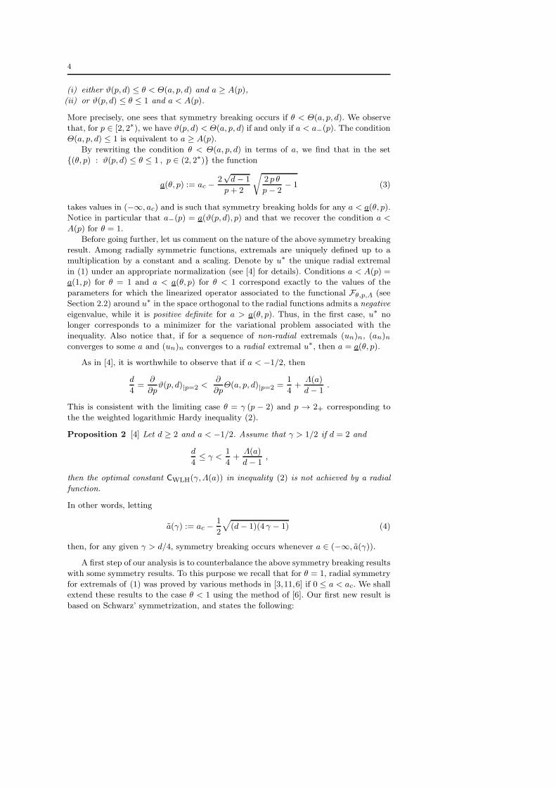
(i) either ϑ(p, d) ≤ θ < Θ(a, p, d) and a ≥ A(p),

(ii) or ϑ(p, d) ≤ θ ≤ 1 and a < A(p).

More precisely, one sees that symmetry breaking occurs if θ < Θ(a, p, d). We observe

that, for p ∈ [2, 2∗), we have ϑ(p, d) < Θ(a, p, d) if and only if a < a−(p). The condition

Θ(a, p, d) ≤ 1 is equivalent to a ≥ A(p).

By rewriting the condition θ < Θ(a, p, d) in terms of a, we find that in the set

{(θ, p) : ϑ(p, d) ≤ θ ≤ 1 , p ∈ (2, 2∗)} the function

a(θ, p) := ac −2√d− 1

p + 2

√

2 p θ

p− 2− 1 (3)

takes values in (−∞, ac) and is such that symmetry breaking holds for any a < a(θ, p).

Notice in particular that a−(p) = a(ϑ(p, d), p) and that we recover the condition a <

A(p) for θ = 1.

Before going further, let us comment on the nature of the above symmetry breaking

result. Among radially symmetric functions, extremals are uniquely defined up to a

multiplication by a constant and a scaling. Denote by u∗ the unique radial extremal

in (1) under an appropriate normalization (see [4] for details). Conditions a < A(p) =

a(1, p) for θ = 1 and a < a(θ, p) for θ < 1 correspond exactly to the values of the

parameters for which the linearized operator associated to the functional Fθ,p,Λ (see

Section 2.2) around u∗ in the space orthogonal to the radial functions admits a negative

eigenvalue, while it is positive definite for a > a(θ, p). Thus, in the first case, u∗ no

longer corresponds to a minimizer for the variational problem associated with the

inequality. Also notice that, if for a sequence of non-radial extremals (un)n, (an)nconverges to some a and (un)n converges to a radial extremal u∗, then a = a(θ, p).

As in [4], it is worthwhile to observe that if a < −1/2, then

d

4=

∂

∂pϑ(p, d)|p=2 <

∂

∂pΘ(a, p, d)|p=2 =

1

4+

Λ(a)

d− 1.

This is consistent with the limiting case θ = γ (p − 2) and p → 2+ corresponding to

the the weighted logarithmic Hardy inequality (2).

Proposition 2 [4] Let d ≥ 2 and a < −1/2. Assume that γ > 1/2 if d = 2 and

d

4≤ γ <

1

4+

Λ(a)

d− 1,

then the optimal constant CWLH(γ, Λ(a)) in inequality (2) is not achieved by a radial

function.

In other words, letting

a(γ) := ac −1

2

√

(d− 1)(4 γ − 1) (4)

then, for any given γ > d/4, symmetry breaking occurs whenever a ∈ (−∞, a(γ)).

A first step of our analysis is to counterbalance the above symmetry breaking results

with some symmetry results. To this purpose we recall that for θ = 1, radial symmetry

for extremals of (1) was proved by various methods in [3,11,6] if 0 ≤ a < ac. We shall

extend these results to the case θ < 1 using the method of [6]. Our first new result is

based on Schwarz’ symmetrization, and states the following:

5

Theorem 2 For any d ≥ 3, p ∈ (2, 2∗), there is a curve θ 7→ a(θ, p) such that, for any

a ∈ [a(θ, p), ac), CCKN(θ, p, Λ(a)) = C∗CKN(θ, p, Λ(a)). Moreover, limθ→1− a(θ, p) = 0,

and limθ→0+ a(θ, p) = ac.

At this point, d = 2 is not covered and we have no corresponding result for the weighted

logarithmic Hardy inequality. Actually, numerical computations (see Fig. 1) do not

indicate that our method, which is based on Schwarz’ symmetrization, could eventually

apply to the logarithmic Hardy inequality.

As for the case θ = 1, d ≥ 2, where symmetry is known to hold for (1) in a neigh-

borhood of a = 0−, for b > 0: see [12,13,14,7,6], the symmetry result of Theorem 2 is

far from sharp. Indeed, for θ = 1, it has recently been proved in [6] that symmetry also

holds for p in a neighborhood of 2+, and that there is a continuous curve p 7→ a(p)

such that symmetry holds for any a ∈ (a(p), ac), while extremals are not radially sym-

metric if a ∈ (−∞, a(p)). We shall extend this result to the more general interpolation

inequalities (1) and to (2).

Notice that establishing radial symmetry in the case 0 < θ < 1 in (1) poses a more

delicate problem than when θ = 1, because of the term ‖|x|−(a+1) u‖2 (1−θ)

L2(Rd)

. Nonethe-

less, by adapting the arguments of [6], we shall prove that a continuous surface splits

the set of parameters into two sets that identify respectively the symmetry and sym-

metry breaking regions. The case d = 2 is also covered, while it was not in Theorem 2.

Theorem 3 For all d ≥ 2, there exists a continuous function a∗ defined on the set

{(θ, p) ∈ (0, 1]×(2, 2∗) : θ > ϑ(p, d)} with values in (−∞, ac) such that limp→2+

a∗(θ, p) =

−∞ and

(i) If (a, p) ∈ (a∗(θ, p), ac) × (2, 2∗), (1) has only radially symmetric extremals.

(ii) If (a, p) ∈ (−∞, a∗(θ, p))× (2, 2∗), none of the extremals of (1) is radially symmet-

ric.

(iii) For every p ∈ (2, 2∗), a(θ, p) ≤ a∗(θ, p) ≤ a(θ, p) < ac.

Surprisingly, the symmetry in the regime a → ac appears as a consequence of the

asymptotic behavior of the extremals in (1) for θ = 1 as a → −∞, which has been

established in [2]. Symmetry holds as p → 2+ for reasons which are similar to the ones

found in [6].

Concerning the weighted logarithmic Hardy inequality (2), we observe that it can

be obtained as the limiting case of inequality (1) as p → 2+, provided θ = γ (p − 2).

Actually, in this limit, the inequality degenerates into an equality, so that (2) is obtained

by differentiating both sides of the inequality with respect to p at p = 2. It is therefore

remarkable that symmetry and symmetry breaking results can be extended to (2),

which is a kind of first order correction to Hardy’s inequality. Inequality (2) has been

established recently and so far no symmetry results were known for its extremals. Here

is our first main result:

Theorem 4 Let d ≥ 2, there exists a continuous function a∗∗ : (d/4,∞) → (−∞, ac)

such that for any γ > d/4 and a ∈ [a∗∗(γ), ac), there is a radially symmetric extremal

for (2), while for a < a∗∗(γ) no extremal of (2) is radially symmetric. Moreover,

a∗∗(γ) ≥ a(γ) for any γ ∈ (d/4,∞).

6

Theorems 3 and 4 do not allow to decide whether (θ, p) 7→ a∗(θ, p) and γ 7→ a∗∗(γ)

coincide with (θ, p) 7→ a(θ, p) and γ 7→ a(γ) given by (3) and (4) respectively. If the set

of non-radial extremals bifurcates from the set of radial extremals, then a∗ = a in case

of (1) and a∗∗ = a in case of (2). Moreover, most of the known symmetry breaking

results rely on linearization and the method developed in [6] for proving symmetry

and applied in Theorems 3 and 4 also relies on linearization. It would therefore be

tempting to conjecture that a∗ = a and a∗∗ = a. It turns out that this is not the case.

We are now going to establish a new symmetry breaking phenomenon, outside the zone

of instability of the radial extremal, i.e. when a > a, for some values of θ < 1 for (1)

and for some a > a(γ) in case of (2). These are striking results, as they clearly depart

from previous methods.

Theorem 5 Let d ≥ 2. There exists η > 0 such that for every p ∈ (2, 2+η) there exists

an ε > 0 with the property that for θ ∈ [ϑ(p, d), ϑ(p, d)+ε) and a ∈ [a(θ, p),a(θ, p)+ε),

no extremal for (1) corresponding to the parameters (θ, p, a) is radially symmetric.

Notice that there is always an extremal function for (1) if θ > ϑ(p, d), and also in some

cases if θ = ϑ(p, d). See [5] for details. The plots in Fig. 2 provide a value for η.

We have a similar statement for logarithmic Hardy inequalities, which is our third

main result. Let

ΛSB(γ, d) :=1

8(4 γ − 1) e

(

π4 γ−d−1

16

)1

4 γ−1(

dγ

)4 γ

4 γ−1 Γ(

d2

)

24 γ−1 . (5)

Theorem 6 Let d ≥ 2 and assume that γ > 1/2 if d = 2. If Λ(a) > ΛSB(γ, d),

then there is symmetry breaking: no extremal for (2) corresponding to the parameters

(γ, a) is radially symmetric. As a consequence, there exists an ε > 0 such that, if

a ∈ [a(γ), a(γ) + ε) and γ ∈ [d/4, d/4 + ε), with γ > 1/2 if d = 2, there is symmetry

breaking.

This result improves the one of Proposition 2, at least for γ in a neighborhood of

(d/4)+. Actually, the range of γ for which ΛSB(γ, d) < Λ(γ) can be deduced from

our estimates, although explicit expressions are hard to read. See Fig. 4 and further

comments at the end of Section 5.

This paper is organized as follows. Section 2 is devoted to preliminaries (Emden-

Fowler transform, symmetry breaking results based on the linear instability of radial

extremals) and to the proof of Theorem 2 using Schwarz’ symmetrisation. Sections 3

and 4 are devoted to the proofs of Theorems 3 and 4 respectively. Theorems 5 and 6

are established in Section 5.

2 Preliminaries

2.1 The Emden-Fowler transformation

Consider the Emden-Fowler transformation

u(x) = |x|−(d−2−2a)/2w(y) where y = (s, ω) ∈ R× Sd−1 =: C ,

x ∈ Rd, s = − log |x| ∈ R and ω = x/|x| ∈ S

d−1 .

7

The scaling invariance in Rd becomes a translation invariance in the cylinder C, in the

s-direction, and radial symmetry for a function in Rd becomes dependence on the s-

variable only. Also, invariance under a certain Kelvin transformation in Rd corresponds

to the symmetry s 7→ −s in C. More precisely, a radially symmetric function u on Rd,

invariant under the Kelvin transformation u(x) 7→ |x|2 (a−ac) u(x/|x|2), corresponds to

a function w on C which depends only on s and satisfies w(−s) = w(s). We shall call

such a function a s-symmetric function.

Under this transformation, (1) can be stated just as an interpolation inequality in

H1(C). Namely, for any w ∈ H1(C),

‖w‖2 Lp(C) ≤ CCKN(θ, p,Λ)

(

‖∇w‖2 L2(C) + Λ ‖w‖2 L2

(C)

)θ‖w‖2 (1−θ)

L2(C)

(6)

with Λ = Λ(a) = (ac − a)2. With these notations, recall that

Λ = 0 ⇐⇒ a = ac and Λ > 0 ⇐⇒ a < ac .

At this point it becomes clear that a < ac or a > ac plays no role and only the value

of Λ > 0 matters. Similarly, by the Emden-Fowler transformation, (2) becomes

∫

C|w|2 log |w|2 dy ≤ 2 γ log

[

CWLH(γ, Λ)(

‖∇w‖2 L2(C) + Λ

)]

, (7)

for any w ∈ H1(C) normalized by ‖w‖2 L2

(C) = 1, for any d ≥ 1, a < ac, γ ≥ d/4, and

γ > 1/2 if d = 2.

2.2 Linear instability of radial extremals

Symmetry breaking for extremals of (7) has been discussed in detail for θ = 1 in [2,9],

and by the same methods in [4], where symmetry breaking has been established also

when θ ∈ (0, 1). The method goes as follows. Consider an extremal w∗ for (6) among

s-symmetric functions. It realizes a minimum for the functional

Fθ,p,Λ[w] :=

(

‖∇w‖2 L2

(C) + Λ ‖w‖2 L2

(C)

)

‖w‖21−θθ

L2(C)

‖w‖2/θ Lp(C)

(8)

among functions depending only on s and Fθ,p,Λ[w∗] = C∗CKN(θ, p,Λ)−1/θ. Once the

maximum of w∗ is fixed at s = 0, since w∗ solves an autonomous ordinary differential

equation, by uniqueness, it automatically satisfies the symmetry w∗(−s) = w∗(s) for

any s ∈ R. Next, one linearizes Fθ,p,Λ around w∗. This gives rise to a linear operator,

whose kernel is generated by dw∗/ds and which admits a negative eigenvalue in H1(C)

if and only if a < a(θ, p), that is for

Λ > Λ(θ, p) := (ac − a(θ, p))2 ,

where the function a(θ, p) is defined in (3). Hence, if a < a(θ, p), it is clear that

Fθ,p,Λ − Fθ,p,Λ[w∗] takes negative values in a neighbourhood of w∗ in H1(C) and

extremals for (6) cannot be s-symmetric, even up to translations in the s-direction. By

the Emden-Fowler transformation, extremals for (1) cannot be radially symmetric.

8

Remark 1 Theorem 5 asserts that there are cases where a > a(θ, p), so that the ex-

tremal s-symmetric function w∗ is stable in H1(C), but for which symmetry is broken,

in the sense that we prove C∗CKN(θ, p, Λ) < CCKN(θ, p, Λ). This will be studied in

Section 5.

In the case of the weighted logarithmic Hardy inequality, symmetry breaking can

be investigated as in [4] by studying the linearization of the functional

Gγ,Λ[w] :=‖∇w‖2

L2(C) + Λ ‖w‖2

L2(C)

‖w‖2 L2

(C)exp

{

12 γ

∫

Cw2

‖w‖2

L2(C)

log

(

w2

‖w‖2

L2(C)

)

dy

} . (9)

around an s-symmetric extremal w∗. In this way one finds that extremals for inequal-

ity (7) are not s-symmetric whenever d ≥ 2,

Λ > Λ(γ) :=1

4(d− 1)(4 γ − 1) = Λ(a(γ)) .

2.3 Proof of Theorem 2

As in [6], we shall prove Theorem 2 by Schwarz’ symmetrization after rephrasing (1)

as follows. To u ∈ D1,2a (Rd), we may associate the function v ∈ D1,2

0 (Rd) by setting:

u(x) = |x|a v(x) ∀ x ∈ Rd .

Inequality (1) is then equivalent to

‖|x|a−b v‖2 Lp(Rd) ≤ CCKN(θ, p, Λ) (A− λB)θ B1−θ

with A := ‖∇v‖2 L2

(Rd), B := ‖|x|−1 v‖2

L2(Rd)

and λ := a (2 ac − a). We observe that

the function B 7→ h(B) := (A− λB)θ B1−θ satisfies

h′(B)

h(B)=

1 − θ

B − λ θ

A− λB .

By Hardy’s inequality, we know that

A− λB ≥ infa>0

(

A− a (2 ac − a)B)

= A− a2c B > 0

for any v ∈ D1,20 (Rd) \ {0}. As a consequence, h′(B) ≤ 0 if

(1 − θ)A < λB . (10)

If this is the case, Schwarz’ symmetrization applied to v decreases A, increases B, and

therefore decreases (A− λB)θ B1−θ, while it increases ‖|x|a−b v‖2 Lp(Rd)

. Optimality

in (1) is then reached among radial functions. Notice that λ > 0 is required by our

method and hence only the case ac > 0, i.e. d ≥ 3, is covered.

Let

t :=AB − a2c .

9

Condition (10) amounts to

t ≤ θ a2c − (ac − a)2

1 − θ. (11)

If u is a minimizer for (1), it has been established in [5, Lemma 3.4] that

(t + Λ)θ ≤ (CCKN(1, 2∗, a2c))ϑ(d,p)

C∗CKN(θ, p, 1)

(ac − a)2 θ− 2dϑ(p,d)

(

t+ a2c

)ϑ(d,p). (12)

For completeness, we shall briefly sketch the proof of (12) below in Remark 5. The

two conditions (11) and (12) determine two upper bounds for t, which are respectively

monotone decreasing and monotone increasing in terms of a. As a consequence, they

are simultaneously satisfied if and only if a ∈ [a0, ac), where a0 is determined by the

equality case in (11) and (12). See Fig. 1. This completes the proof of Theorem 2. ⊓⊔

0.2 0.4 0.6 0.8 1 1.2 1.4

0.2

0.4

0.6

0.8

1

Fig. 1 According to the proof of Theorem 2, symmetry holds if a ∈ [a0(θ, p), ac), θ ∈(ϑ(p, d), 1). The curves θ 7→ a0(θ, p) are parametrized by θ ∈ [ϑ(p, d), 1), with d = 5, ac = 1.5and p = 2.1, 2.2, . . . 3.2. Horizontal segments correspond to θ = ϑ(p, d), a0(θ, p) ≤ a < ac.

Remark 2 Although this is not needed for the proof of Theorem 2, to understand why

symmetry can be expected as a → ac, it is enlightening to consider the moving planes

method. With the above notations, if u is an extremal for (1), then v is a solution of

the Euler-Lagrange equation

− θ

A− λB ∆v +

(

1 − θ

B − θ λ

A− λB

)

v

|x|2 =vp−1

‖|x|−(b−a) v‖p Lp

(Rd)

.

If d = 2, then λ = −a2 < 0 and 1−θB − θ λ

A−λB is always positive. If d ≥ 3, 1−θB − θ λ

A−λBis negative if and only if (10) holds. Assume that this is the case. Using the Emden-

Fowler transformation defined in Section 2.1, we know that the corresponding solution

on the cylinder is smooth, so that v has no singularity except maybe at x = 0. We

10

can then use the moving planes technique and prove that v is radially symmetric by

adapting the results of [10,8].

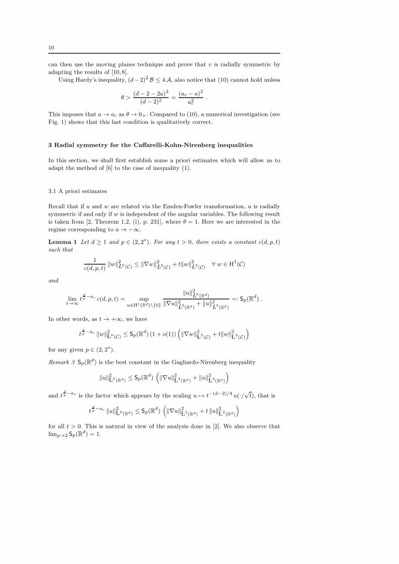
Using Hardy’s inequality, (d−2)2 B ≤ 4A, also notice that (10) cannot hold unless

θ >(d− 2 − 2a)2

(d− 2)2=

(ac − a)2

a2c.

This imposes that a → ac as θ → 0+. Compared to (10), a numerical investigation (see

Fig. 1) shows that this last condition is qualitatively correct.

3 Radial symmetry for the Caffarelli-Kohn-Nirenberg inequalities

In this section, we shall first establish some a priori estimates which will allow us to

adapt the method of [6] to the case of inequality (1).

3.1 A priori estimates

Recall that if u and w are related via the Emden-Fowler transformation, u is radially

symmetric if and only if w is independent of the angular variables. The following result

is taken from [2, Theorem 1.2, (i), p. 231], where θ = 1. Here we are interested in the

regime corresponding to a → −∞.

Lemma 1 Let d ≥ 1 and p ∈ (2, 2∗). For any t > 0, there exists a constant c(d, p, t)

such that

1

c(d, p, t)‖w‖2 Lp

(C) ≤ ‖∇w‖2 L2(C) + t‖w‖2 L2

(C) ∀ w ∈ H1(C)

and

limt→∞

tdp−ac c(d, p, t) = sup

u∈H1(Rd)\{0}

‖u‖2 Lp(Rd)

‖∇u‖2 L2

(Rd)+ ‖u‖2

L2(Rd)

=: Sp(Rd) .

In other words, as t → +∞, we have

tdp−ac ‖w‖2 Lp

(C) ≤ Sp(Rd) (1 + o(1))(

‖∇w‖2 L2(C) + t‖w‖2 L2

(C)

)

for any given p ∈ (2, 2∗).

Remark 3 Sp(Rd) is the best constant in the Gagliardo-Nirenberg inequality

‖u‖2 Lp(Rd) ≤ Sp(Rd)

(

‖∇u‖2 L2(Rd)

+ ‖u‖2 L2(Rd)

)

and tdp−ac is the factor which appears by the scaling u 7→ t−(d−2)/4 u(·/

√t), that is

tdp−ac ‖u‖2 Lp

(Rd) ≤ Sp(Rd)(

‖∇u‖2 L2(Rd)

+ t ‖u‖2 L2(Rd)

)

for all t > 0. This is natural in view of the analysis done in [2]. We also observe that

limp→2 Sp(Rd) = 1.

11

From Lemma 1, we can actually deduce that the asymptotic behavior of c(d, p, t) as

t → ∞ is uniform in the limit p → 2.

Corollary 1 Let d ≥ 1 and q ∈ (2, 2∗). For any p ∈ [2, q],

c(d, p, t) ≤ t−ζ [c(d, q, t)]1−ζ ∀ t > 0

with ζ =2 (q−p)p (q−2)

. As a consequence,

limt→∞

supp∈[2,q]

tdp−ac c(d, p, t) ≤

[

Sq(Rd)]

q (p−2)p (q−2)

.

Proof Using the trivial estimate

‖w‖2 L2(C) ≤

1

t

[

‖∇w‖2 L2(C) + t ‖w‖2 L2

(C)

]

,

the estimate of Lemma 1

‖w‖2 Lq(C) ≤ c(d, q, t)

[

‖∇w‖2 L2(C) + t ‖w‖2 L2

(C)

]

and Holder’s interpolation: ‖w‖ Lp(C) ≤ ‖w‖ζ

L2(C)

‖w‖1−ζ

Lq(C), we easily get the first

estimate. Sincedp − ac − ζ = (1 − ζ)

(

dq − ac

)

,

we find

tdp−ac c(d, p, t) ≤

(

tdq−ac c(d, q, t)

)1−ζ.

and the second estimate follows. ⊓⊔

Remark 4 Notice that for d ≥ 3, the second estimate in Corollary 1 also holds with

q = 2∗ and ζ = 1 − ϑ(p, d). In such a case, we can actually prove that

c(d, p, t) ≤ tac− dp (ϑ(p, d)S∗(d))ϑ(p,d) (1 − ϑ(p, d))1−ϑ(p,d)

where S∗(d) = CCKN(1, 2∗, a2c) is the optimal constant in Sobolev’s inequality: for any

u ∈ H1(Rd), ‖u‖2 L2∗

(Rd)≤ S∗(d)‖∇u‖2

L2(Rd)

.

Consider the functional Fθ,p,Λ defined by (8) on H1(C). A minimizer exists for any

p > 2 if d = 1 or d = 2, and p ∈ (2, 2∗) if d ≥ 3. See [2] for details if θ = 1 and [5,

Theorem 1.3 (ii)] if θ ∈ (ϑ(p, d), 1). The special, limiting case θ = ϑ(p, 1) is discussed

in [4] if d = 1 and in [5] if d ≥ 1. From now on, we denote by w = wθ,p,Λ an extremal

for (6), whenever it exists, that is, a minimizer for Fθ,p,Λ. It satisfies the following

Euler-Lagrange equations,

−θ∆w + ((1 − θ) t + Λ)w = (t + Λ)1−θ wp−1

with t := ‖∇w‖2 L2

(C)/‖w‖2 L2

(C), when we assume the normalization condition

(

‖∇w‖2 L2(C) + Λ ‖w‖2 L2

(C)

)θ‖w‖2 (1−θ)

L2(C)

= ‖w‖p Lp

(C) .

12

Such a condition can always be achieved by homogeneity and implies

‖w‖p−2

Lp(C) =

1

CCKN(θ, p, Λ). (13)

As a consequence of the Euler-Lagrange equations, we also have

‖∇w‖2 L2(C) + Λ ‖w‖2 L2

(C) = (t + Λ)1−θ ‖w‖p Lp

(C) . (14)

Remark 5 If w is a minimizer for Fθ,p,Λ, then we know that

(t + Λ)θ ‖w‖2 L2(C) =

‖w‖2 Lp(C)

CCKN(θ, p,Λ)≤

‖w‖2 Lp(C)

C∗CKN(θ, p, Λ)

=‖w‖2 Lp

(C)C∗CKN(θ, p, 1)

Λθ−p−22 p .

On the other hand, by Holder’s inequality: ‖w‖ Lp(C) ≤ ‖w‖ϑ(d,p)

L2∗(C)

‖w‖1−ϑ(d,p)

L2(C)

, and by

Sobolev’s inequality (cf. Remark 4) written on the cylinder, we know that

‖w‖2 Lp(C) ≤ (S∗(d))ϑ(p,d)‖w‖2ϑ(d,p)

L2∗(C)

‖w‖2 (1−ϑ(d,p))

L2(C)

= (S∗(d))ϑ(p,d)(

‖∇w‖2 L2(C) + a2c ‖w‖2 L2

(C)

)ϑ(p,d)‖w‖2 (1−ϑ(p,d))

L2(C)

= (S∗(d))ϑ(p,d)(

t + a2c

)ϑ(p,d)‖w‖2 L2

(C) .

Collecting the two estimates proves (12) for v(x) = |x|−ac w(s, ω), where s = − log |x|and ω = x/|x|, for any x ∈ R

d (Emden-Fowler transformation written for a = 0).

As in [2], we can assume that the extremal w = wθ,p,Λ depends only on s and on

an azimuthal angle φ ∈ (0, π) of the sphere, and thus satisfies

− θ(

∂ssw + Dφ (∂φw))

+ ((1 − θ) t + Λ)w = (t + Λ)1−θ wp−1 . (15)

Here we denote by ∂sw and ∂φw the partial derivatives with respect to s and φ re-

spectively, and by Dφ the derivative defined by: Dφw := (sinφ)2−d ∂φ((sinφ)d−2w).

Moreover, using the translation invariance of (6) in the s-variable, the invariance of the

functional Fθ,p,Λ under the transformation (s, ω) 7→ (−s, ω) and the sliding method,

we can also assume without restriction that w is such that

w(s, φ) = w(−s, φ) ∀ (s, φ) ∈ R× (0, π) ,

∂sw(s, φ) < 0 ∀ (s, φ) ∈ (0,+∞) × (0, π) ,

maxCw = w(0, φ0) ,

(16)

for some φ0 ∈ [0, π]. In particular notice that

‖∇w‖2 L2(C) = ωd−2

∫ +∞

0

∫ π

0

(

|∂sw|2 + |∂φw|2)

(sinφ)d−2 dφds

where ωd−2 is the area of Sd−2. From Lemma 1, we obtain the following estimate:

13

Corollary 2 Assume that d ≥ 2, Λ > 0, p ∈ (2, 2∗) and θ ∈ (ϑ(p, d), 1). Let t =

t(θ, p,Λ) be the maximal value of ‖∇w‖2 L2

(C)/‖w‖2 L2

(C) among all extremals of (6).

Then t(θ, p,Λ) is bounded from above and moreover

lim supp→2+

t(θ, p, Λ) < ∞ and lim supΛ→0+

t(θ, p, Λ) < ∞ ,

where the limits above are taken respectively for Λ > 0 and θ ∈ (0, 1) fixed, and for

p ∈ (2, 2∗) and θ ∈ (ϑ(p, d), 1) fixed.

Proof Let tn := ‖∇wn‖2 L2(C)/‖wn‖2 L2

(C), where wn are extremals of (6) with Λ =

Λn ∈ (0,+∞), p = pn ∈ (2, 2∗) and θ ∈ (0, 1]. We shall be concerned with one of the

following regimes:

(i) Λn = Λ and pn = p do not depend on n ∈ N, and θ ∈ (ϑ(p, d), 1),

(ii) Λn = Λ does not depend on n ∈ N, θ ∈ (0, 1] and limn→∞ pn = 2,

(iii) pn = p does not depend on n ∈ N, θ ∈ [ϑ(p, d), 1] and limn→∞ Λn = 0.

Assume that limn→∞ tn = ∞, consider (14) and apply Lemma 1 to get

tdpn

−ac

nmin{θ,1−θ}Spn (Rd)

(1 + o(1)) ≤ (tn + Λn)1−θ ‖wn‖pn−2

Lpn(C) =(tn + Λn)1−θ

CCKN(θ, pn, Λn)(17)

where we have used the assumption that 1 − ϑ(pn, d) = dpn

− ac > 1 − θ. This gives a

contradiction in case (i).

Using the fact that

CCKN(θ, p, Λ) ≥ C∗CKN(θ, p, Λ)

where C∗CKN(θ, p,Λ) is the best constant in (1) among radial functions given in Sec-

tion 1, and observing that

C∗CKN(θ, p, Λ) = C

∗CKN(θ, p, 1)Λ

p−22 p

−θ ,

we get

1/C∗CKN(θ, p,Λ) ∼ Λθ−p−2

2 p → 0 as Λ → 0 .

In case (iii), if we assume that tn → +∞, then this provides a contradiction with (17).

In case (ii), we know that

limp→2+

C∗CKN(θ, p,Λ) = Λ−θ

and, by (17) and Lemma 1,

td

pn−ac

nmin{θ, 1 − θ}

Spn(Rd)(1 + o(1)) ≤ (tn + Λ)1−θ

C∗CKN(θ, pn, Λ)

= Λθ t1−θn (1 + o(1))

as n → ∞. Again this provides a contradiction in case we assume limn→∞

tn = ∞. ⊓⊔

Let k(p,Λ) := C∗CKN(θ = 1, p, Λ) and recall that k(p,Λ) = Λ−(p+2)/(2 p) k(p, 1) and

limp→2+ k(p, 1) = 1. As a consequence of the symmetry result in [6], we have

14

Lemma 2 There exists a positive continuous function ε on (2, 2∗) with

limp→2

ε(p) = ∞ and limp→2∗

ε(p) = a−(p+2)/pc k(2∗, 1)

such that, for any p ∈ (2, 2∗),

‖w‖2 Lp(C) ≤ ε ‖∇w‖2 L2

(C) + Z(ε, p) ‖w‖2 L2(C) ∀ w ∈ H1(C)

holds for any ε ∈ (0, ε(p)) with Z(ε, p) := ε−p−2p+2 k(p, 1)

2 pp+2 .

Proof From [6], we know that there exists a continuous function λ : (2, 2∗) → (a2c ,∞)

such that limp→2 λ(p) = ∞, limp→2∗ λ(p) = a2c and, for any λ ∈ (0, λ(p)], the inequality

‖w‖2 Lp(C) ≤ k(p, λ)

(

‖∇w‖2 L2(C) + λ ‖w‖2 L2

(C)

)

∀ w ∈ H1(C)

holds true. Therefore, letting

ε(p) := k(p, λ(p)) = λ(p)−(p+2)/(2 p)k(p, 1) ,

our estimate holds with λ = λ(p), ε = λ−(p+2)/(2 p) k(p, 1) and Z(ε, p) = ε λ. ⊓⊔

Lemma 3 Assume that d ≥ 2, p ∈ (2, 2∗) and θ ∈ [ϑ(p, d), 1]. If w is an extremal

function of (6) and if w is not s-symmetric, then

θ (d− 1) + (1 − θ) t + Λ < (t + Λ)1−θ(p− 1) ‖w‖p−2

L∞(C) . (18)

Proof Let w be an extremal for (6), normalized so that (16) holds. We denote by

φ ∈ (0, π) the azimuthal coordinate on Sd−1. By the Poincare inequality in S

d−1, we

know that:∫

Sd−1

|Dφ(∂φw)|2 dω ≥ (d− 1)

∫

Sd−1

|(∂φw)|2 dω

while, by multiplying the equation in (15) by Dφ(∂φw), after obvious integration by

parts, we find:

θ

(∫

C

(

∣

∣∂s(

∂φw)∣

∣

2+∣

∣Dφ

(

∂φw)∣

∣

2)

dy

)

+ ((1 − θ) t + Λ)

∫

C

∣

∣∂φw∣

∣

2dy

= (t+Λ)1−θ (p−1)

∫

Cwp−2

∣

∣∂φw∣

∣

2dy ≤ (t+Λ)1−θ (p−1) ‖w‖p−2

L∞(C)

∫

C

∣

∣∂φw∣

∣

2dy .

By combining the two above estimates, the conclusion holds if ‖∂φw‖ L2(C) 6= 0. ⊓⊔

15

3.2 The critical regime: approaching a = ac

Proposition 3 Assume that d ≥ 2, p ∈ (2, 2∗) and θ ∈ [ϑ(p, d), 1]. Let (Λn)n be a

sequence converging to 0+ and let (wn)n be a sequence of extremals for (6), satisfy-

ing the normalization condition (13). Then both tn := ‖∇wn‖2 L2(C)/‖wn‖2 L2

(C) and

‖wn‖ L∞(C) converge to 0 as n → +∞.

Proof First of all notice that, under the given assumption, we can use the results in

[5, Theorem 1.3 (i)] in order to ensure the existence of an extremal for (6) even for

θ = ϑ(p, d). Moreover with the notations of Corollary 2, we know that (tn)n is bounded

and, by (13) and (14),

‖∇wn‖2 L2(C) + Λn ‖wn‖2 L2

(C) =(tn + Λn)1−θ

CCKN(θ, p,Λn)p/(p−2)

with CCKN(θ, p, Λn)−p/(p−2) ≤ C∗CKN(θ, p,Λn)−p/(p−2) ∼ Λ

θ pp−2− 1

2n → 0 as Λn → 0+,

where we have used the fact that θ pp−2 − 1

2 > 0 for θ ≥ ϑ(p, d). Thus, using (13) we have

limn→∞

‖∇wn‖ L2(C) = 0 and lim

n→∞‖wn‖ Lp

(C) = 0. Hence, (wn)n converges to w ≡ 0,

weakly in H1loc(C) and also in C1,α

loc for some α ∈ (0, 1). By (16), it follows

limn→∞

‖wn‖ L∞(C) = 0 .

Now, let t∞ := limn→∞ tn and assume by contradiction that t∞ > 0. The function

Wn = wn/‖wn‖H1(Rd) solves

−θ ∆Wn + ((1 − θ) tn + Λn)Wn = (tn + Λn)1−θ wp−2n Wn .

Multiply the above equation by Wn and integrate on C, to get

θ ‖∇Wn‖2 L2(C) + ((1 − θ) t∞(1 + o(1)) + Λn) ‖Wn‖2 L2

(C)

≤ (t∞(1 + o(1)) + Λn)1−θ ‖wn‖p−2

L∞(C) ‖Wn‖2 L2

(C) .

This is in contradiction with the fact that ‖Wn‖H1(Rd) = 1, for any n ∈ N. ⊓⊔

Corollary 3 Assume that d ≥ 2, p ∈ (2, 2∗) and θ ∈ [ϑ(p, d), 1]. There exists ε =

ε(θ, p) > 0 such that extremals of (6) are s-symmetric for every 0 < Λ < ε.

Proof Any sequence (wn)n as in Proposition 3 violates (18) for n large enough, unless

∂φwn ≡ 0. The conclusion readily follows. ⊓⊔

3.3 The Hardy regime: approaching p = 2

We proceed similarly as in Proposition 3 and Corollary 3.

Proposition 4 Assume that d ≥ 2, fix Λ > 0 and θ ∈ (0, 1]. There exists η ∈(0, 4 θ/(d− 2 θ)) such that all extremals of (6) are s-symmetric if p ∈ (2, 2 + η).

16

Proof The case θ = 1 is already established in [6]. So, for fixed Λ > 0 and 0 < θ < 1,

let wn be an extremal of (6) with p = pn → 2+. By Corollary 2, we know that (tn)nis bounded and

‖∇wn‖2 L2(C) + Λ ‖wn‖2 L2

(C) = (tn + Λ)1−θ ‖wn‖pn−2

Lpn (C) ‖wn‖2 Lpn(C) .

First we prove that tn converges to 0 as n → +∞. Assume by contradiction that

limn→∞ tn = t > 0 after extracting a subsequence if necessary, and choose ε ∈ (0, 1/Λ)

so that

(t + Λ)θ > Λθ (ε t + 1) . (19)

Recalling that C∗CKN(θ, p,Λ) ∼ Λ−θ as p → 2+, we find that

‖wn‖pn−2

Lpn(C) = 1/CCKN(θ, pn, Λ) ≤ 1/C∗CKN(θ, pn, Λ) → Λθ .

Using Lemma 2 to estimate ‖wn‖2 Lpn(C) by ε ‖∇w‖2 L2

(C)+Z(ε, p) ‖w‖2 L2

(C), for n large

enough, we get

(tn + Λ) ‖wn‖2 L2(C)

= ‖∇wn‖2 L2(C) + Λ ‖wn‖2 L2

(C) = (tn + Λ)1−θ ‖wn‖pn−2

Lpn(C) ‖wn‖2 Lpn (C)

≤ (tn + Λ)1−θ Λθ (1 + o(1)) (ε tn + Z(ε, pn, d)) ‖wn‖2 L2(C) .

Hence, by passing to the limit as n → ∞, and using the fact that

limn→∞

Z(ε, pn, d) = 1 ,

we deduce that

(t + Λ) ≤ (t + Λ)1−θ Λθ (ε t + 1)

in contradiction with (19). This proves that limn→+∞ tn = 0.

Summarizing, wn is a solution of

−θ∆wn + ((1 − θ) tn + Λ)wn = (tn + Λ)1−θ wpn−1n

such that tn = ‖∇wn‖2 L2(C)/‖wn‖2 L2

(C) → 0 as n → +∞. Let cn := ‖wn‖ Lpn(C) and

Wn := wn/cn. We know that

cpn−2n =

1

CCKN(θ, pn, Λ)≤ 1

C∗CKN(θ, pn, Λ)

→ Λθ

and

‖∇Wn‖2 L2(C) + Λ ‖Wn‖2 L2

(C) = (tn + Λ)1−θ cpn−2n ‖Wn‖pn

Lpn(C) = (tn + Λ)1−θ cpn−2n .

Hence we have

limn→∞

‖∇Wn‖2 L2(C) + Λ ‖Wn‖2 L2

(C) = limn→∞

(tn + Λ)1−θ cpn−2n ≤ Λ .

Furthermore, from limn→∞ tn = 0, we deduce that limn→∞ ‖∇Wn‖2 L2(C) = 0 and

lim supn→∞ ‖Wn‖2 L2(C) ≤ 1. This proves that (Wn)n is bounded in H1(C) and that,

17

up to subsequences, its weak limit is 0. By elliptic estimates and (16), we conclude that

lim supn→∞ ‖Wn‖ L∞(C) = 0. Therefore, lim supn→∞ ‖Wn‖pn−2

L∞(C) ≤ 1.

We can summarize the properties we have obtained so far for an extremal wn of (6)

with p = pn → 2+ as follows:

limn→∞

tn = 0 and lim supn→∞

‖wn‖pn−2

Lpn(C) ≤ Λθ .

Incidentally, by means of the maximum principle for (15), we also get that

‖wn‖pn−2

L∞(C) ≥

(1 − θ) tn + Λ

(tn + Λ)1−θ≥ Λθ ,

which establishes that

limn→∞

‖wn‖pn−2

L∞(C) = Λθ .

Inequality (18) is clearly violated for n large enough unless ∂φwn ≡ 0. This concludes

the proof. ⊓⊔

3.4 A reformulation of Theorem 3 on the cylinder. Scalings and consequences

As in [6], it is convenient to rewrite Theorem 3 using the Emden-Fowler transformation.

Theorem 7 For all d ≥ 2, there exists a continuous function Λ∗ defined on the set

{(θ, p) ∈ (0, 1]×(2, 2∗) : θ ≥ ϑ(p, d)} with values in (0,+∞) such that limp→2+

Λ∗(θ, p) =

+∞ and

(i) If (Λ, p) ∈ (0, Λ∗(θ, p)) × (2, 2∗), then (1) has only s-symmetric extremals.

(ii) If Λ = Λ∗(θ, p), then CCKN(θ, p,Λ) = C∗CKN(θ, p, Λ).

(iii) If (Λ, p) ∈ (Λ∗(θ, p),+∞) × (2, 2∗), none of the extremals of (1) is s-symmetric.

(iv) 0 < Λ∗(θ, p) ≤ Λ(θ, p).

Notice that s-symmetric and non s-symmetric extremals may coexist in case (ii). In (iv),

we use the notation Λ(θ, p) = (ac−a(θ, p))2, where the function a(θ, p) is defined in (3).

A key step for the proof of Theorem 7 relies on scalings in the s variable of the

cylinder. If w ∈ H1(C) \ {0}, let wσ(s, ω) := w(σ s, ω) for σ > 0. A simple calculation

shows that

Fθ,p,σ2Λ[wσ ] = σ2− 1θ+ 2

p θ Fθ,p,Λ[w]−σ2− 1θ+ 2

p θ (σ2−1)‖∇ωw‖2

L2(C) ‖w‖2

1−θθ

L2(C)

‖w‖2/θ Lp

(C)

. (20)

As a consequence, we observe that

C∗CKN(θ, p, σ2Λ)−

1θ = Fθ,p,σ2Λ[w∗

θ,p,σ2Λ]

= σ2− 1θ+ 2

p θ C∗CKN(θ, p, Λ)−

1θ = σ2− 1

θ+ 2

p θ Fθ,p,Λ[w∗θ,p,Λ] .

Lemma 4 If d ≥ 2, Λ > 0 and p ∈ (2, 2∗), then the following holds:

18

(i) If CCKN(θ, p, Λ) = C∗CKN(θ, p, Λ), then CCKN(θ, p, λ) = C∗

CKN(θ, p, λ) and, after a

proper normalization, wθ,p,λ = w∗θ,p,λ for any λ ∈ (0, Λ).

(ii) If there is an extremal wθ,p,Λ, which is not s-symmetric, even up to translations in

the s-direction, then CCKN(θ, p, λ) > C∗CKN(θ, p, λ) for all λ > Λ.

Recall that, according to [4], the extremal w∗θ,p,λ among s-symmetric functions is

uniquely defined up to translations in the s variable, multiplications by a constant

and scalings with respect to s. We assume that it is normalized in such a way that it

is uniquely defined. As for non s-symmetric minimizers, we have no uniqueness result.

With a slightly loose notation, we shall write wθ,p,λ for an extremal, but the reader

has to keep in mind that, eventually, we pick one extremal among several, which are

not necessarily related by one of the above transformations.

Proof To prove (i), apply (20) with wσ = wθ,p,λ, λ = σ2Λ, 0 < σ < 1 and w(s, ω) =

wθ,p,λ(s/σ, ω):

1

CCKN(θ, p, λ)1θ

= Fθ,p,λ[wθ,p,λ]

= σ2− 1θ+ 2

p θ Fθ,p,Λ[w] + σ− 1θ+ 2

p θ (1 − σ2)‖∇ωw‖2

L2(C) ‖w‖2

1−θθ

L2(C)

‖w‖2/θ Lp

(C)

≥ σ2− 1θ+ 2

p θ

C∗CKN(θ, p, Λ) 1θ

+ σ− 1θ+ 2

p θ (1 − σ2)‖∇ωw‖2

L2(C) ‖w‖2

1−θθ

L2(C)

‖w‖2/θ Lp

(C)

=1

C∗CKN(θ, p, λ)

1θ

+ σ− 1θ+ 2

p θ (1 − σ2)‖∇ωw‖2

L2(C) ‖w‖2

1−θθ

L2(C)

‖w‖2/θ Lp

(C)

.

By definition, CCKN(θ, p, λ) ≥ C∗CKN(θ, p, λ) and from the above inequality we find

that necessarily ∇ωw ≡ 0, and the first claim follows.

Assume that wθ,p,Λ is an extremal with explicit dependence in ω and apply (20)

with w = wθ,p,Λ, wσ(s, ω) := w(σ s, ω), λ = σ2Λ and σ > 1:

1

CCKN(θ, p, λ)1θ

≤ Fθ,p,σ2Λ[wσ ]

=σ2− 1

θ+ 2

p θ

CCKN(θ, p, λ)1θ

− σ− 1θ+ 2

p θ (σ2 − 1)‖∇ωwθ,p,Λ‖2 L2

(C)‖wθ,p,Λ‖2 1−θ

θ

L2(C)

‖wθ,p,Λ‖2/θ Lp(C)

≤ σ2− 1θ+ 2

p θ

C∗CKN(θ, p, Λ)

1θ

− σ− 1θ+ 2

p θ (σ2 − 1)‖∇ωwθ,p,Λ‖2 L2

(C)‖wθ,p,Λ‖2 1−θ

θ

L2(C)

‖wθ,p,Λ‖2/θ Lp(C)

< C∗CKN(θ, p, λ)−

1θ ,

since ∇ωwθ,p,Λ 6≡ 0. This proves the second claim. ⊓⊔

19

By virtue of Corollary 3, we know that, for p ∈ (2, 2∗) and ϑ(p, d) ≤ θ ≤ 1, the set

{Λ > 0 : Fθ,p,Λ has only s-symmetric minimizers} is not empty, and hence we can

define:

Λ∗(θ, p) := sup {Λ > 0 : Fθ,p,Λ has only s-symmetric minimizers} .

In particular, by Proposition 1 (also see Section 2.2), Lemma 4 and Proposition 4, we

have:

0 < Λ∗(θ, p) ≤ Λ(θ, p) and limp→2+

Λ∗(θ, p) = +∞ .

Corollary 4 With the above definition of Λ∗(θ, p), we have:

(i) if λ ∈ (0, Λ∗(θ, p)), then CCKN(θ, p, λ) = C∗CKN(θ, p, λ) and, after a proper normal-

ization, wθ,p,λ = w∗θ,p,λ,

(ii) if λ = Λ∗(θ, p), then CCKN(θ, p, λ) = C∗CKN(θ, p, λ),

(iii) if λ > Λ∗(θ, p) and θ > ϑ(p, d), then CCKN(θ, p, λ) > C∗CKN(θ, p, λ).

Proof (i) is a consequence of Lemma 4 (i). It is easy to check that CCKN(θ, p, λ) is

a non-increasing function of λ. By considering limλ→Λ+Fθ,p,Λ[w∗

θ,p,λ], we get (ii). If

p ∈ (2, 2∗) and θ ∈ (ϑ(p, d), 1], it has been shown in [5] that Fθ,p,Λ always attains its

minimum in H1(C) \ {0}, so that (iii) follows from Lemma 4 (ii). ⊓⊔

3.5 The proof of Theorem 7

In case θ = ϑ(p, d), extremals might not exist: see [5]. To complete the proof of Theorem

7, we have to prove that the property of Lemma 4 (iii) also holds if θ = ϑ(p, d) and to

establish the continuity of Λ∗.

Lemma 5 If λ > Λ∗(θ, p) and θ = ϑ(p, d), then CCKN(θ, p, λ) > C∗CKN(θ, p, λ).

Proof Consider the Gagliardo-Nirenberg inequality

‖u‖2 Lp(Rd) ≤ CGN(p) ‖∇u‖2ϑ(p,d)

L2(Rd)

‖u‖2 (1−ϑ(p,d))

L2(Rd)

∀ u ∈ H1(Rd) (21)

and assume that CGN(p) is the optimal constant. According to [5] (see Lemma 6 below

for more details), we know that

CGN(p) ≤ CCKN(ϑ(p, d), p, λ) .

According to [5, Theorem 1.4 (i)] there are extremals for (6) with θ = ϑ(p, d), p ∈(2, 2∗) and λ > 0, whenever the above inequality is strict. By Corollary 4 (ii) we know

that CGN(p) ≤ C∗CKN(ϑ(p, d), p, λ) if λ = Λ∗(ϑ(p, d), p).

Case 1: Assume that CGN(p) = C∗CKN(ϑ(p, d), p, Λ∗(ϑ(p, d), p)). Then for all λ >

Λ∗(ϑ(p, d), p),

C∗CKN(ϑ(p, d), p, λ) < CGN(p) ≤ CCKN(ϑ(p, d), p, λ)

because C∗CKN(θ, p, λ) is decreasing in λ, which proves the result.

20

Case 2: Assume that CGN(p) < C∗CKN(ϑ(p, d), p,Λ∗(ϑ(p, d), p)). We can always choose

λ > Λ∗(ϑ(p, d), p), sufficiently close to Λ∗(ϑ(p, d), p), so that

CGN(p) < C∗CKN(ϑ(p, d), p, λ) ≤ CCKN(ϑ(p, d), p, λ) .

Then [5, Theorem 1.4 (i)] ensures the existence of an extremal wθ,p,λ of (6) with

θ = ϑ(p, d). By the definition of Λ∗(ϑ(p, d), p), such an extremal is non s-symmetric.

The result follows from Lemma 4 (ii). ⊓⊔

To complete the proof of Theorem 7, we only need to establish the continuity of

Λ∗ with respect to the parameters (θ, p) with p ∈ (2, 2∗) and ϑ(p, d) ≤ θ < 1. The

argument is similar to the one used in [6] for the case θ = 1. First of all, by using the

definition of Λ∗(θ, p), Lemma 4 (i) and the s-symmetric extremals, it is easy to see

that, for any sequences (θn)n and (pn)n such that θn → θ and pn → p ∈ (2, 2∗),

lim supn→>+∞

Λ∗(θn, pn) ≤ Λ∗(θ, p) .

To see that equality actually holds, we argue by contradiction and assume that for a

given sequence θn ∈ [ϑ(pn, d), 1] and pn ∈ (2, 2∗), we have:

Λ∞ := limn→+∞

Λ∗(θn, pn) < Λ∗(θ, p) .

For n large, fix λ such that Λ∗(θn, pn) < λ < Λ∗(θ, p) ≤ Λ(θ, p).

If θ > ϑ(p, d), then θn > ϑ(pn, d) for n large, and we find a sequence of non

s-symmetric extremals wθn,pn,λ that, along a subsequence, must converge to an s-

symmetric extremal w∗θ,p,Λ, a contradiction with λ < Λ(θ, p) as already noted in the

introduction.

If θ = ϑ(p, d), then, by strict monotonicity of C∗CKN with respect to λ, we find:

CGN(p) ≤ C∗CKN(ϑ(p, d), p, Λ∗(p, d)) < C∗

CKN(ϑ(p, d), p, λ) and so, for n sufficiently

large: CGN(p) < C∗CKN(θn, pn, λ) ≤ CCKN(θn, pn, λ). Again by [5, Theorem 1.4 (i)],

there exist non s-symmetric extremals wθn,pn,λ of (6) relative to the parameters

(θn, pn, λ), that, along a subsequence, must converge to an extremal of (6) relative to

the parameters (θ, p,Λ). Since λ < Λ∗(θ, p), the limiting extremal must be s-symmetric

and we obtain a contradiction as above. This completes the proof of Theorem 7. ⊓⊔

Remark 6 As already noticed above, at Λ = Λ∗(θ, p), we have

CCKN(θ, p,Λ∗(θ, p)) = C∗CKN(θ, p, Λ∗(θ, p))

and, as long as there are extremal functions, either Λ∗(θ, p) = Λ(θ, p), or a s-symmetric

extremal and a non s-symmetric one may coexist. This is precisely what occurs in the

framework of Theorem 5, at least for θ > ϑ(p, d).

4 Radial symmetry for the weighted logarithmic Hardy inequalities

As in Section 3.4, we rephrase Theorem 4 on the cylinder.

Theorem 8 For all d ≥ 2, there exists a continuous function Λ∗∗ defined on the

set {γ > d/4} and with values in (0,+∞) such that for all Λ ∈ (0, Λ∗∗(γ)], there

is an s-symmetric extremal of (2), while for any Λ > Λ∗∗(γ), no extremal of (7) is

s-symmetric. Moreover, Λ∗∗(γ) ≤ 14 (4 γ − 1) (d− 1) = Λ(γ).

21

4.1 The critical regime: approaching Λ = 0

In order to prove the above theorem, we first start by showing that for γ > d/4 and Λ

close to 0, the extremals for (7) are s-symmetric. From [5, Theorem 1.3 (ii)], we know

that such extremals exist.

Proposition 5 Let γ > d/4 and d ≥ 2. Then, for Λ > 0 sufficiently small, any

extremal wγ,Λ of (7) is s-symmetric.

Proof Let us consider γ > d/4 and a sequence of positive numbers (Λn)n converging

to 0. Let us denote by (wn)n a sequence of extremals for (7) with parameter Λn.

For simplicity, let us normalize the functions wn so that ‖wn‖ L2(C) = 1. Moreover,

we can assume that wn = wn depends only on s and the azimuthal angle φ ∈ Sd−1

and maxC wn = wn(0, φ0) for some φ0 ∈ [0, π]. Finally, wn is a minimum for Gθ,p,Λ

defined in (9), and we have Gθ,p,Λ[wn] = 1/Cn with Cn := CWLH(γ, Λn) for any n ∈ N.

Therefore wn satisfies the Euler-Lagrange equation

−∆wn − C−1n wn (1 + log |wn|2) exp

(

1

2 γ

∫

C|wn|2 log |wn|2 dy

)

= µn wn (22)

for some µn ∈ R. Multiplying this equation by wn and integrating by parts we get

‖∇wn‖2 L2(C) − C

−1n exp

(

1

2 γ

∫

C|wn|2 log |wn|2 dy

)∫

Cw2n (1 + log |wn|2) dy = µn .

(23)

In addition, the condition Gθ,p,Λ[wn] = 1/Cn gives

‖∇wn‖2 L2(C) + Λn = C

−1n exp

(

1

2 γ

∫

C|wn|2 log |wn|2 dy

)

.

As in [5], consider Holder’s inequality, ‖w‖ Lq(C) ≤ ‖w‖ζ

L2(C)

‖w‖1−ζ

Lp(C) with ζ =

2 (p − q)/(q (p − 2)) for any q such that 2 ≤ q ≤ p ≤ 2∗. For q = 2, this inequality

becomes an equality, with ζ = 1, so that we can differentiate with respect to q at q = 2

and obtain

∫

C|w|2 log

(

|w|2‖w‖2

L2(C)

)

dy ≤ pp−2 ‖w‖2 L2

(C) log(‖w‖2

Lp(C)

‖w‖2

L2(C)

)

.

Let CGN(p) be the best constant in (21). Combining the two inequalities, we obtain

the following logarithmic Sobolev inequality on the cylinder: for all d ≥ 1,

∫

Cw2 log

w2

‖w‖2 L2

(C)

dy ≤ d

2‖w‖2 L2

(C) log

‖∇w‖2 L2

(C)‖w‖2

L2(C)

+K(d) ‖w‖2 L2(C) , (24)

where

K(d) := infp∈(2,2∗)

p

p− 2CGN(p) .

See [4, Lemma 5] for more details and a sharp version, but not in Weissler’s logarithmic

form as it is here, of the logarithmic Sobolev inequality on the cylinder.

22

Applying this inequality to wn, we obtain

‖∇wn‖2 L2(C) + Λn ≤ C

−1n e

K(d)2 γ

(

‖∇wn‖2 L2(C)

)d4 γ

.

Since γ > d/4, Λn → 0 and Cn → +∞ (see [4, Theorem B’]), we see that (∇wn)nconverges to 0 as n → +∞. On the other hand, ‖wn‖ L2

(C) = 1, so, up to subsequences,

(wn)n converges weakly and in C2,αloc to w ≡ 0.

Now, like in the proofs of Corollary 3 by using (22), we see that the function

χn := Dφwn satisfies:

∫

C(

|∂sχn|2 + |∂φχn|2)

dy

− C−1n exp

(

12 γ

∫

C |wn|2 log |wn|2 dy)

∫

C |χn|2 (3 + 2 log |wn|2) dy

= µn ‖χn‖2 L2(C) . (25)

Hence, by means of the Poincare inequality we derive

(d− 1 − µn) ‖χn‖2 L2(C)

≤ C−1n exp

(

12 γ

∫

C |wn|2 log |wn|2 dy)

∫

C |χn|2 (3 + 2 log wn) dy

≤ C−1n exp

(

12 γ

∫

C |wn|2 log |wn|2 dy)

‖χn‖2 L2(C) (3 + 2 log (‖wn‖ L∞

(C))) ≤ 0

for n large, since ‖wn‖ L∞(C) converges to 0 as n → +∞. Next observe that by the

strong convergence of (∇wn)n to 0 in L2(Rd) (23) and by the logarithmic Sobolev

inequality (24), we obtain limn→∞ µn = 0. So, necessarily χn ≡ 0 for n large and the

proof is complete. ⊓⊔

4.2 The proof of Theorem 8

Consider the functional Gγ,Λ defined in (9). If w ∈ H1(C)\{0}, let wσ(s, ω) := w(σ s, ω)

for any σ > 0. A simple calculation shows that for all σ > 0,

Gγ,σ2 Λ[wσ ] = σ2− 12 γ Gγ,Λ[w]−

(σ2 − 1) σ− 12 γ ‖∇ωw‖2

L2(C)

‖w‖2 L2

(C)exp

{

12 γ

∫

Cw2

‖w‖2

L2(C)

log

(

w2

‖w‖2

L2(C)

)

dy

} .

The above expression is the counterpart of (20) in the case of the weighted logarithmic

Hardy inequality and we can even observe that 2 − 12 γ = limp→2+(2 − 1

θ + 2p θ ) when

θ = γ (p − 2). We use it exactly as in Section 3.4 to prove that for any d ≥ 2, Λ > 0

and γ > d/4, the following properties hold:

(i) If CCKN(γ, Λ) = C∗WLH(γ,Λ), then CCKN(γ, λ) = C∗

WLH(γ, λ) and, after a proper

normalization, wγ,λ = w∗γ,λ, for any λ ∈ (0, Λ).

(ii) If there is there is an extremal wγ,Λ, which is not s-symmetric, even up to trans-

lations in the s-direction, then CWLH(γ, λ) > C∗WLH(γ, λ) for all λ > Λ.

23

At this point, in view of Proposition 5 and by recalling the role of the function a in

(4), we can argue as in Section 3.5 to prove the existence of a continuous function Λ∗∗

defined on (d/4,∞), such that

(i) 0 < Λ∗∗(γ) < Λ(γ),

(ii) if λ ∈ (0, Λ∗(γ)), then CWLH(γ, λ) = C∗WLH(γ, λ) and, after a proper normalization,

wγ,λ = w∗γ,λ,

(iii) if λ = Λ∗∗(γ), then CWLH(γ, λ) = C∗WLH(γ, λ),

(iv) if λ > Λ∗∗(γ), then CWLH(γ, λ) > C∗WLH(γ, λ).

This concludes the proof of Theorems 8. ⊓⊔

5 New symmetry breaking results

This section is devoted to the proof of Theorems 5 and 6. We prove symmetry breaking

in the range of parameters where the radial extremal is a strict, local minimum for

the variational problem associated to inequalities (1) and (2). Consider the optimal

constants in the limit cases given respectively by θ = ϑ(p, d) and γ = d/4. We recall

that

1

CCKN(ϑ(p, d), p, Λ)= inf

u∈D1,2a (Rd)\{0}

‖|x|−a ∇u‖2ϑ(p,d)

L2(Rd)

‖|x|−(a+1) u‖2 (1−ϑ(p,d))

L2(Rd)

‖|x|−b u‖2 Lp

(Rd)

and

1

CWLH(d/4, Λ)= inf ‖|x|−a ∇u‖2 L2

(Rd)exp

[

− 2d

∫

Rd

|u|2|x|2 (a+1) log

(

|x|2 (ac−a) |u|2)

dx

]

where the last infimum is taken on the set of the functions u ∈ D1,2a (Rd) such that

‖|x|− (a+1) u‖ L2(Rd)

= 1. We also define the best constants in Gagliardo-Nirenberg and

logaritmic Sobolev inequalities respectively by

1

CGN(p):= inf

u∈H1(Rd)\{0}

‖∇u‖2ϑ(p,d)

L2(Rd)

‖u‖2 (1−ϑ(p,d))

L2(Rd)

‖u‖2 Lp

(Rd)

and1

CLS:= inf

u∈H1(Rd)‖u‖ L2

(Rd)=1

∫

Rd

|∇u|2 dx exp

[

− 2d

∫

Rd

|u|2 log |u|2 dx

]

It is well known (see for instance [15]) that CLS = 2π d e .

Lemma 6 Let d ≥ 3 and p ∈ (2, 2∗). For all a < ac, we have

CGN(p) ≤ CCKN(ϑ(p, d), p,Λ) and CLS ≤ CWLH(d/4, Λ) .

If d = 2, the first inequality still holds while the second one is replaced by CLS ≤lim supγ→(1/2)+ CWLH(γ, Λ).

24

Proof Consider an extremal u for either the Gagliardo-Nirenberg or the logaritmic

Sobolev inequality. It is known that such a solution exists, is unique up to multiplication

by constants, translations and scalings (in case of the logaritmic Sobolev inequalities,

take for instance u(x) = (2π)−d/4 exp(−|x|2/4) for any x ∈ Rd). Let e ∈ S

d−1 and use

un(x) := u(x + n e), n ∈ N, as a sequence of test functions for the quotients defining

CCKN(ϑ(p, d), p, Λ) and CWLH(d/4, Λ) respectively. We first use the reformulation of

(1) used in Section 2.3 in terms of v(x) = |x|−a u(x), and observe that, for θ = ϑ(p, d) =

1 − (b− a), d ≥ 2, we have

1

CCKN(θ, p, Λ)

= infv∈H1(Rd)\{0}

(

‖∇v‖2 L2

(Rd)+ a (a− 2 ac) ‖|x|−1 v‖2

L2(Rd)

)θ‖|x|−1 v‖2 (1−θ)

L2(Rd)

‖|x|θ−1 v‖2 Lp

(Rd)

≤

(

‖∇un‖2 L2(Rd)

+ a (a− 2 ac) ‖|x|−1 un‖2 L2(Rd)

)θ‖|x|−1 un‖2 (1−θ)

L2(Rd)

‖|x|θ−1 un‖2 Lp(Rd)

=

(

‖∇u‖2 L2

(Rd)+

a (a−2 ac)n2 ‖| xn − e|−1 u‖2

L2(Rd)

)θ‖| xn − e|−1 u‖2 (1−θ)

L2(Rd)

‖| xn − e|1−θ u‖2 Lp

(Rd)

−→n→+∞

(

‖∇u‖2 L2

(Rd)

)θ‖u‖2 (1−θ)

L2(Rd)

‖u‖2 Lp

(Rd)

=1

CGN(p).

The inequality CLS ≤ CWLH(d/4, Λ) follows from a similar computation if d ≥ 3. If

d = 2, it is enough to repeat the computation for a well chosen sequence (γn)n such

that γn > 1/2 for any n ∈ N and limn→∞ γn = 1/2. ⊓⊔

Proof of Theorem 5. Let g(x) := (2π)−d/4 exp(−|x|2/4) for any x ∈ Rd and consider

the function

h(p, d) :=‖∇g‖2ϑ(p,d)

L2(Rd)

‖g‖2 (1−ϑ(p,d))

L2(Rd)

‖g‖2 Lp

(Rd)

.

A tedious but elementary computation provides an explicit value for h(p, d) in terms

of Γ functions, that can be used to get the estimate

1

CCKN(ϑ(p, d), p,Λ(a−(p)))≤ 1

CGN(p)≤ h(p, d)

where a−(p) = a(ϑ(p, d), p). Consider the function

L(p, d) := h(p, d)C∗CKN

(

ϑ(p, d), p, Λ(a−(p)))

.

Explicit computations show that limp→2+ L(p, d) = 1 and ℓ(d) := limp→2+∂ L

∂p (p, d)

is an increasing function of d such that limd→∞ ℓ(d) = − 14 log 2 < 0. Hence, for any

given d ≥ 2, there exists an η > 0 such that L(p, d) < 1 for any p ∈ (2, 2 + η). See

Fig. 2. As a consequence, we have

h(p, d) <1

C∗CKN(ϑ(p, d), p,Λ(a−(p)))

25

provided 0 < p − 2 < η, with η small enough, thus proving that C∗CKN(θ, p,Λ) <

CCKN(θ, p, Λ) if θ = ϑ(p, d) and a = a−(p). By continuity and according to Theorem 7

(ii), the strict inequality also holds for θ close to ϑ(p, d) and a close to a−(p), as

claimed. ⊓⊔

2.2 2.4 2.6 2.8 3 3.2

0.96

0.98

1.02

1.04

1.06

Fig. 2 Plots of L(p, d) as a function of p for d = 3, . . . 10.

Proof of Theorem 6. For the weighted logarithmic Hardy inequality (2), the same

method applies. From the explicit estimates of CLS and C∗WLH(γ, Λ), it is a tedious

but straightforward computation to check that C∗WLH(γ, Λ) < CLS if and only if

Λ(a) > ΛSB(γ, d), where ΛSB has been defined in (5). As a special case, notice that

C∗WLH(d/4, Λ(−1/2)) < CLS if d ≥ 3, while, for d = 2, we have:

limγ→(1/2)+

C∗WLH(γ, Λ(−1/2)) < CLS .

See Fig. 3. By continuity, the inequality C∗WLH(γ, Λ(γ)) < CLS remains valid for γ >

d/4, provided γ − d/4 > 0 is small enough. This completes the proof. ⊓⊔

Remark 7 The condition CLS < C∗WLH(d/4, Λ) amounts to a ∈ (a⋆, ac) for some ex-

plicit a⋆ and from [5, Theorem 1.4] we know that this is a sufficient condition for the

existence of an extremal function for (2). The symmetry breaking results of Theorem 6

hold for any a ∈ (−∞, a⋆). In that case, the existence of an extremal for (2) is not

known if γ = d/4, d ≥ 3, but it is granted by [5, Theorem 1.3] for any γ > d/4, d ≥ 2.

Compared with the result in Proposition 2, we see by numerical calculations that

Λ(a) > Λ(γ) is more restrictive than Λ(a) > ΛSB(γ, d) except if d = 2 and γ ∈[0.621414 . . . , 6.69625 . . .], d = 3 and γ ∈ [0.937725 . . . , 4.14851 . . .], or d = 4 and

γ ∈ [1.31303 . . . , 2.98835 . . .]. For d ≥ 5, we observe that ΛSB(γ, d) < Λ(γ). See Fig. 4.

As a concluding remark for the weighted logarithmic Hardy inequality, we em-

phasize the fact that, in many cases, the comparison with the logarithmic Sobolev

inequality gives better informations about the symmetry breaking properties of the

extremals than methods based on a linearization approach.

26

5 10 15 20 25 30 35

0.84

0.86

0.88

0.92

0.94

0.96

0.98

Fig. 3 Plot of C∗

WLH(d/4, Λ(−1/2))/CLS in terms of d ∈ N, d ≥ 3.

2 4 6 8 10

0.5

0.75

1.25

1.5

1.75

2

Fig. 4 Plot of ΛSB(γ, d)/Λ(γ) as a function of γ, for d = 2, 3, . . . 6.

Acknowledgements This work has been partially supported by the projects CBDif andEVOL of the French National Research Agency (ANR) and by the FIRB-ideas project “Anal-ysis and beyond”.

c© 2010 by the authors. This paper may be reproduced, in its entirety, for non-commercialpurposes.

References

1. L. Caffarelli, R. Kohn, and L. Nirenberg, First order interpolation inequalities withweights, Compositio Math., 53 (1984), pp. 259–275.

2. F. Catrina and Z.-Q. Wang, On the Caffarelli-Kohn-Nirenberg inequalities: sharp con-stants, existence (and nonexistence), and symmetry of extremal functions, Comm. PureAppl. Math., 54 (2001), pp. 229–258.

27

3. K. S. Chou and C. W. Chu, On the best constant for a weighted Sobolev-Hardy inequality,J. London Math. Soc. (2), 48 (1993), pp. 137–151.

4. M. Del Pino, J. Dolbeault, S. Filippas, and A. Tertikas, A logarithmic Hardy in-equality, Journal of Functional Analysis, 259 (2010), pp. 2045 – 2072.

5. J. Dolbeault and M. J. Esteban, Extremal functions for Caffarelli-Kohn-Nirenberg andlogarithmic Hardy inequalities. Preprint, 2010.

6. J. Dolbeault, M. J. Esteban, M. Loss, and G. Tarantello, On the symmetry ofextremals for the Caffarelli-Kohn-Nirenberg inequalities, Adv. Nonlinear Stud., 9 (2009),pp. 713–726.

7. J. Dolbeault, M. J. Esteban, and G. Tarantello, The role of Onofri type inequalitiesin the symmetry properties of extremals for Caffarelli-Kohn-Nirenberg inequalities, in twospace dimensions, Ann. Sc. Norm. Super. Pisa Cl. Sci. (5), 7 (2008), pp. 313–341.

8. M. J. Esteban and M. Ramaswamy, Nonexistence result for positive solutions of non-linear elliptic degenerate problems, Nonlinear Anal., 26 (1996), pp. 835–843.

9. V. Felli and M. Schneider, Perturbation results of critical elliptic equations ofCaffarelli-Kohn-Nirenberg type, J. Differential Equations, 191 (2003), pp. 121–142.

10. B. Gidas, W. M. Ni, and L. Nirenberg, Symmetry of positive solutions of nonlinearelliptic equations in Rn, in Mathematical analysis and applications, Part A, vol. 7 of Adv.in Math. Suppl. Stud., Academic Press, New York, 1981, pp. 369–402.

11. T. Horiuchi, Best constant in weighted Sobolev inequality with weights being powers ofdistance from the origin, J. Inequal. Appl., 1 (1997), pp. 275–292.

12. C.-S. Lin and Z.-Q. Wang, Erratum to: “Symmetry of extremal functions for theCaffarelli-Kohn-Nirenberg inequalities” [Proc. Amer. Math. Soc. 132 (2004), no. 6, 1685–1691], Proc. Amer. Math. Soc., 132 (2004), p. 2183 (electronic).

13. , Symmetry of extremal functions for the Caffarrelli-Kohn-Nirenberg inequalities,Proc. Amer. Math. Soc., 132 (2004), pp. 1685–1691 (electronic).

14. D. Smets and M. Willem, Partial symmetry and asymptotic behavior for some ellipticvariational problems, Calc. Var. Partial Differential Equations, 18 (2003), pp. 57–75.

15. F. B. Weissler, Logarithmic Sobolev inequalities for the heat-diffusion semigroup, Trans.Amer. Math. Soc., 237 (1978), pp. 255–269.