Convexity Preserving Interpolation
181
CONVEXITY PRESERVING INTERPOLATION – Stationary Nonlinear Subdivision and Splines
-
Upload
khangminh22 -
Category
Documents
-
view
0 -
download
0
Transcript of Convexity Preserving Interpolation

CONVEXITY PRESERVING
INTERPOLATION
–
Stationary Nonlinear Subdivision and Splines

Cover: M.C. Escher’s ”Convex en Concaaf” c© 1998 Cordon Art – Baarn – Holland.Alle rechten voorbehouden.
The research described in this thesis was part of the research program TWI44.3411of the Dutch Technology Foundation STW and was carried out at the University ofTwente, Enschede, The Netherlands.
Convexity Preserving Interpolation – Stationary Nonlinear Subdivision and Splines –/ Kuijt, Frans / 1998, 171 p. : ill. ; 25 cmThesis University of Twente, Enschede, The Netherlands.- With ref. - With summary in Dutch.ISBN 90-365-1201-8
Copyright c© 1998 by F. KuijtFaculty of Mathematical SciencesUniversity of TwenteP.O. Box 217NL-7500 AE EnschedeThe Netherlands

CONVEXITY PRESERVING
INTERPOLATION
–
Stationary Nonlinear Subdivision and Splines
PROEFSCHRIFT
ter verkrijging vande graad van doctor aan de Universiteit Twente,
op gezag van de rector magnificus,prof. dr. F.A. van Vught,
volgens besluit van het College voor Promotiesin het openbaar te verdedigen
op vrijdag 9 oktober 1998 te 15.00 uur
door
Frans Kuijt
geboren op 4 februari 1971te Epe

Dit proefschrift is goedgekeurd door de promotor en de assistent-promotor:
Prof. dr. C.R. TraasDr. R.M.J. van Damme

Toen zag ik al het werk Gods, dat de mens niet kanuitvinden, het werk, dat onder de zon geschiedt, om
hetwelk een mens arbeidt om te zoeken, maar hij zal hetniet uitvinden; ja, indien ook een wijze zeide, dat hij
het zou weten, zo zal hij het toch niet kunnen uitvinden.
(Prediker 8:17)


Contents
1 Introduction 1
2 Splines, Subdivision Schemes and Shape Preservation 9
2.1 Definitions . . . . . . . . . . . . . . . . . . . . . . . . . . . . . . . . . . . 92.1.1 Basic definitions . . . . . . . . . . . . . . . . . . . . . . . . . . . 92.1.2 Interpolation and approximation . . . . . . . . . . . . . . . . . . 112.1.3 Shape preservation . . . . . . . . . . . . . . . . . . . . . . . . . . 122.1.4 Shape preserving interpolation . . . . . . . . . . . . . . . . . . . 15
2.2 Splines . . . . . . . . . . . . . . . . . . . . . . . . . . . . . . . . . . . . . 152.2.1 Introduction to splines . . . . . . . . . . . . . . . . . . . . . . . . 152.2.2 Spline interpolation . . . . . . . . . . . . . . . . . . . . . . . . . 182.2.3 Splines and shape preservation . . . . . . . . . . . . . . . . . . . 20
2.3 Subdivision . . . . . . . . . . . . . . . . . . . . . . . . . . . . . . . . . . 252.3.1 From splines to subdivision . . . . . . . . . . . . . . . . . . . . . 262.3.2 Approximating subdivision schemes and shape preservation . . . 282.3.3 Interpolatory subdivision schemes . . . . . . . . . . . . . . . . . 282.3.4 Interpolatory subdivision and shape preservation . . . . . . . . . 292.3.5 Convexity preservation of the linear four-point scheme . . . . . . 30
2.4 Analysis of interpolatory subdivision schemes . . . . . . . . . . . . . . . 32
3 Convexity Preserving Interpolatory Subdivision Schemes 39
3.1 Introduction . . . . . . . . . . . . . . . . . . . . . . . . . . . . . . . . . . 393.2 Problem definition . . . . . . . . . . . . . . . . . . . . . . . . . . . . . . 403.3 Convexity preservation . . . . . . . . . . . . . . . . . . . . . . . . . . . . 423.4 Convergence to a continuously differentiable function . . . . . . . . . . . 443.5 Stability and Approximation order . . . . . . . . . . . . . . . . . . . . . 533.6 Generalisations . . . . . . . . . . . . . . . . . . . . . . . . . . . . . . . . 56

viii Contents
4 Monotonicity Preserving Interpolatory Subdivision Schemes 594.1 Introduction . . . . . . . . . . . . . . . . . . . . . . . . . . . . . . . . . . 594.2 Problem definition . . . . . . . . . . . . . . . . . . . . . . . . . . . . . . 604.3 Monotonicity preservation . . . . . . . . . . . . . . . . . . . . . . . . . . 634.4 Convergence to a continuous function . . . . . . . . . . . . . . . . . . . 644.5 Convergence to a continuously differentiable function . . . . . . . . . . . 654.6 Construction of rational subdivision schemes . . . . . . . . . . . . . . . 684.7 Ratios of first order differences . . . . . . . . . . . . . . . . . . . . . . . 704.8 Convergence of rational subdivision schemes . . . . . . . . . . . . . . . . 744.9 Stability and Approximation order . . . . . . . . . . . . . . . . . . . . . 774.10 Generalisations . . . . . . . . . . . . . . . . . . . . . . . . . . . . . . . . 79
5 Shape Preserving Interpolatory Subdivision Schemes for Nonuniform Data 835.1 Introduction . . . . . . . . . . . . . . . . . . . . . . . . . . . . . . . . . . 835.2 Nonuniform subdivision . . . . . . . . . . . . . . . . . . . . . . . . . . . 84
5.2.1 Problem definition . . . . . . . . . . . . . . . . . . . . . . . . . . 855.2.2 Monotonicity preservation . . . . . . . . . . . . . . . . . . . . . . 855.2.3 Nonuniform subdivision schemes . . . . . . . . . . . . . . . . . . 865.2.4 Example: A nonuniform linear four-point scheme . . . . . . . . . 88
5.3 Convexity preservation . . . . . . . . . . . . . . . . . . . . . . . . . . . . 895.4 Convergence to a continuously differentiable function . . . . . . . . . . . 915.5 Approximation order . . . . . . . . . . . . . . . . . . . . . . . . . . . . . 98
5.5.1 Approximation order of convex subdivision schemes . . . . . . . 985.5.2 Convexity preservation and approximation order four? . . . . . . 995.5.3 Connection with fourth order rational interpolation . . . . . . . . 101
5.6 Midpoint subdivision . . . . . . . . . . . . . . . . . . . . . . . . . . . . . 1015.7 Nonuniform linear subdivision schemes . . . . . . . . . . . . . . . . . . . 102
5.7.1 Introduction . . . . . . . . . . . . . . . . . . . . . . . . . . . . . 1025.7.2 Convergence to a continuously differentiable function . . . . . . . 1035.7.3 Approximation order . . . . . . . . . . . . . . . . . . . . . . . . . 104
5.8 Numerical examples . . . . . . . . . . . . . . . . . . . . . . . . . . . . . 105
6 Shape Preserving C2 Interpolatory Subdivision Schemes 1076.1 Introduction . . . . . . . . . . . . . . . . . . . . . . . . . . . . . . . . . . 1076.2 Problem definition . . . . . . . . . . . . . . . . . . . . . . . . . . . . . . 1086.3 Linear six-point interpolatory subdivision schemes . . . . . . . . . . . . 1106.4 A numerical approach for smoothness analysis . . . . . . . . . . . . . . . 1116.5 Six-point convexity preserving subdivision schemes . . . . . . . . . . . . 1146.6 Six-point monotonicity preserving subdivision schemes . . . . . . . . . . 116

Contents ix
6.6.1 Positivity preserving interpolatory subdivision schemes . . . . . . 1166.6.2 Construction of C2 monotonicity preserving subdivision schemes 118
7 Hermite-Interpolatory Subdivision Schemes 1217.1 Introduction . . . . . . . . . . . . . . . . . . . . . . . . . . . . . . . . . . 1217.2 Hermite-interpolatory subdivision schemes . . . . . . . . . . . . . . . . . 1227.3 Linear Hermite-interpolatory subdivision schemes . . . . . . . . . . . . . 1287.4 Convexity preserving Hermite-interpolatory subdivision schemes . . . . 134
8 A Linear Approach to Shape Preserving Spline Approximation 1418.1 Introduction . . . . . . . . . . . . . . . . . . . . . . . . . . . . . . . . . . 1418.2 Constrained `p-approximation methods . . . . . . . . . . . . . . . . . . 143
8.2.1 Constrained `2-approximation . . . . . . . . . . . . . . . . . . . . 1448.2.2 Constrained `∞-approximation . . . . . . . . . . . . . . . . . . . 1458.2.3 Constrained `1-approximation . . . . . . . . . . . . . . . . . . . . 1458.2.4 Comparison of constrained `p-approximation methods . . . . . . 147
8.3 Linear methods for constrained ’least squares’ . . . . . . . . . . . . . . . 1488.3.1 Constrained `
′p-approximation . . . . . . . . . . . . . . . . . . . . 148
8.3.2 Comparison of constrained `′
p- and `p-approximation . . . . . . . 1498.4 Linear constraints for shape preservation of univariate splines . . . . . . 1508.5 Linear constraints for shape preservation of bivariate splines . . . . . . . 152
8.5.1 Bivariate positivity constraints . . . . . . . . . . . . . . . . . . . 1528.5.2 Bivariate monotonicity constraints . . . . . . . . . . . . . . . . . 1528.5.3 Bivariate convexity constraints . . . . . . . . . . . . . . . . . . . 153
8.6 An iterative algorithm for shape preserving approximation . . . . . . . . 158
References 161
Summary 167
Samenvatting 169
Dankwoord 171

x Contents

Chapter 1
Introduction
Many subjects discussed in this thesis arise from Computer Aided Geometric Design.For example, when measurements are obtained by scanning a three-dimensional object,this often results in a collection of data points located on the surface of such an object.In other problems, measurements performed at a certain physical model supply a dataset. Such a data set is often known to satisfy some qualitative properties. Examplesof such properties are a specific curved behaviour or the knowledge that no oscillationscan occur. Additional conditions can also arise directly from physics: e.g., a quantitylike pressure may not become negative, and an object containing oscillations cannot bepolished in an efficient production process.The way of obtaining measurement data can be very laborious or at least expensive,so only a relatively small number of initial data points is provided in general. As aresult, such an initial data set is too coarse in order to perform accurate calculations orfor visualisation purposes. Therefore, additional data values in between the measuredoriginal values could then be required, i.e., the available data have to be interpolated.However, the interpolant is also required to satisfy the qualitative shape propertiespresent in the initial data.The problem of shape preserving interpolation is important in various problems occur-ring in industry, which is illustrated by practical examples. The first example dealswith the modelling of cars in automobile industry. Similar questions usually arise inaero-plane and ship design.
Car modelling. For modelling a car, its surface can naturally be subdivided into sev-eral parts, and a specific part often has to satisfy certain shape requirements. Someconditions are motivated by the air drag: the resistance of air has to be relativelylow. Other conditions are imposed by strength properties. Beside these technical andphysical conditions, aesthetic requirements play an important role. For example, an

2 1 Introduction
undesired property of a car is that its surface contains wiggles, and the reflection oflight by the sun-shine has to produce nicely shaped images. These visual conditions putsevere constraints on the shape, and the surface of the car is required to be smoothlyshaped without oscillations.
A mathematical way to express this problem is that the interpolating surface at leastis required to be convex. In addition, the surface must be smooth or even curvaturecontinuous. The required smoothness is determined by the application at hand: some-times C1 is sufficient for practical purposes (display of objects in computer graphics,computer vision, robot motion planning, aeroplane design), but sometimes it is not(car design, modelling of lenses). Although smoothness of a function is an attractiveproperty at first sight, one has to take care with this notion of smoothness. Indeed,any function that is only continuous can be approximated arbitrarily well by a functionthat is infinitely times continuously differentiable.Another example to show the requirement of constructing well-shaped surfaces arises indesigning TV-screens. The modelling concerns the shape of the mask that is located ina cathode tube just behind the screen. In this case, a convexity preserving interpolantsatisfying additional curvature constraints is required.
Construction of mask surfaces. The basic principle of a TV-screen is as follows. Forthe three different colours, electron sources shoot three beams in the direction of thescreen. A time-dependent magnetic field deflects these beams in such a way that thewhole screen is scanned. A phosphor dot at the inner-side of the screen will emit lightwhen an electron beam hits it. A mask, consisting of a thin metal plate/foil with smallholes, is placed between the electron sources and the screen, such that each electronbeam hits the right phosphor dot. The distribution of the mask holes slightly deviatesfrom a rectangular pattern. The geometric restrictions on the mask holes are basedon a brightness criterion, determined by optimising the light emission of the phosphordots. Thus, each mask hole is defined by a geometric relation between the electronsources and three phosphor dots.The mask surface modelling requires approximation of the given mask data. Althoughthe customer wants a screen that is as flat as possible, the surface must also satisfysome physical shape requirements: the production process requires the surface to beconvex. Furthermore to improve the strength of the screen and the stability of themask, both the screen and the mask are required to be curved. Flat parts in the masksurface also give rise to oscillations which cause a ’doming-effect’: an electron beamdoes not optimally hit the right phosphor dot, due to a small change in the locationof the mask hole. Taking both aspects into account, a compromise must be proposed.The glass screen must also satisfy some shape requirements. Optical reasons demandthat the screen is both convex and sufficiently smooth, as the screen must be polished.

1 Introduction 3
These examples of shape preserving interpolation problems suggest to formulate theproblem more mathematically as follows:
Given a data set with some characteristic properties.Construct a sufficiently smooth univariate or bivariate function that in-terpolates or approximates these data preserving the same characteristicfeatures.
Methods for data fitting often make use of approximations that can be formulatedas a linear combination of a set of basis functions. Probably the simplest method isobtained by using polynomials, and it is a well-known fact that any univariate data setcan be interpolated by a polynomial which degree is at most the number of data pointsminus one. Although polynomial interpolation generates functions of high smoothness,the interpolants in general oscillate, especially if the number of data points gets larger.These wiggles are not desired in many applications, as they often give rise to physicalincompatibilities, as argued before.Another well-known method suited for many problems concerning interpolation is pro-vided by splines. Splines can be defined as piecewise polynomials that are connected ina smooth way. More freedom for interpolation or approximation is obtained by reduc-ing the smoothness at the connections of neighbouring spline segments. An often-usedunivariate method is interpolation with cubic B-splines: splines of degree three whichare two times continuously differentiable. In practice, these splines appear to be suf-ficiently smooth. Compared to polynomial interpolation, spline interpolation methodsdiminish the occurrence of large oscillations, due to their relatively low degree.Even splines cannot completely avoid unwanted oscillations in some practical problems.Therefore, it is important to incorporate restrictions in the interpolation or approxi-mation method to enforce shape preservation. These restrictions should not reduce thesmoothness of the approximation, which is required to be ‘sufficiently smooth’, as hasbeen remarked earlier.
In this thesis, we examine constrained interpolation methods, and we further restrictto methods that guarantee the preservation of certain shape properties present in thedata, with an emphasis to convexity preservation. This means that the characteristicfeatures treated in this thesis are conditions on the shape of the resulting curve orsurface. The simplest conditions with respect to shape preservation deal with posi-tivity, monotonicity, or convexity preservation. These shape requirements appear asconditions on the derivatives of the interpolant. More general conditions are rangerestrictions, restricted growth, or conditions on the curvature behaviour: this yieldsconditions on derivatives of degree 0, 1, 2, respectively. Other kind of shape conditionsare e.g., curve interpolation with constrained length, but these types of conditions arenot treated in this thesis.

4 1 Introduction
For most applications, it is sufficient when a curve or surface is obtained that satisfiesthe shape constraints and that lies close enough to the given data, i.e., a solution of theconstrained approximation problem. The distance of the solution to the given data, i.e.,the error (in some norm), has to be restricted. The constrained interpolation problem isthen a special case of the approximation problem as the error is required to be zero (inany norm). This is the main reason why we restrict to methods suited for interpolation,or methods that are able to approximate the given data arbitrarily accurate.
Methods for (shape preserving) interpolation or approximation can be classified asfollows:
a. Global methods. A solution is being found on the basis of the solution of a (large)system of equations, often based on a minimisation problem.
b. Local methods. A solution is being found on the basis of information coming froma fixed, relatively small number of neighbouring data points.
The choice whether a global or a local method should be used depends on the applica-tion and the objectives, and, of course, there are important differences:
• Advantages of global interpolation. For many shape preserving interpolation prob-lems, an initial solution is constructed globally by performing a suitable optimi-sation. Another advantage of a global method is that it is often relatively simpleto add shape constraints. An optimisation algorithm can also be extended suchthat the solution satisfies global properties, and an example is minimisation of avariational property like the strain energy.
• Advantages of local interpolation. Locality of an interpolation method is attrac-tive, because a local change in the data, e.g., insertion of additional data, onlyinfluences the solution in a restricted area. As a result, most parts of the solutionbefore changing the data will not be changed. Since no optimisation procedurehas to be performed, local methods do not need large-scale computations or alarge amount of computing time to obtain a solution.
Methods dealing with shape preserving interpolation can also be distinguished in thefollowing classes:
• The usual way to achieve shape preservation is to apply an approximation methodwhich is not especially constructed for the purpose of shape preservation. Theshape is then enforced by additional constraints. A problem that must be treatedcarefully then is the way to introduce additional degrees of freedom, if the dataor the tolerance requires this. For convexity preserving spline interpolation this

1 Introduction 5
occurs in areas where curvature changes rapidly. The way to increase the dimen-sion of the spline space is to increase the degree, or to introduce additional knotsin regions where the data are ’difficult’.
• The second way to incorporate the shape requirements in the construction is touse a method in which the conditions are naturally build-in, i.e., no additionalshape constraints are needed. However, it is not possible to restrict to standardlinear methods like B-splines, since these methods do not preserve shape prop-erties, in general. Examples in this class of methods for the univariate case areshape preserving rational splines, see chapter 2.
Two different research approaches to the problem of shape preserving interpolation andapproximation are discussed in this thesis.The main part of this thesis concerns subdivision. We restrict to local, interpolatorysubdivision schemes for univariate data, which preserve certain shape properties andare necessarily nonlinear. In both classifications, these methods fit in the second class.The research on subdivision is described in the chapters 3-7, and in the papers [KvD97c,KvD98a,KvD97a,KvD97b,KvD98d,KvD98b].The second approach in the final chapter deals with spline methods. We considershape preserving approximation using polynomial splines, and the proposed methodsare global and based on the addition of constraints, see chapter 8 and [KvD98c].
Shape preserving spline approximation. The research contribution to splines dealswith shape preserving spline approximation. Although it is attractive to look for localmethods, note that in case of surfaces most methods from literature that are appli-cable for practical purposes and that preserve convexity are global, however. Theglobal spline approximation method proposed in this thesis deals with a given scat-tered univariate or bivariate data set which possesses certain shape properties, suchas convexity, monotonicity, or range restrictions. The data are approximated by forexample bivariate tensor-product B-splines preserving the shape characteristics presentin the data.Shape preservation of the spline approximant is obtained by additional constraints, andthe attractiveness of the algorithm lies in the linearity of the shape constraints. Thegeneral (necessary and sufficient) conditions for convexity or monotonicity, are nonlin-ear in the unknowns, and therefore hard to incorporate in an optimisation procedure.Sufficient shape constraints are constructed which are local linear sufficient conditionsin the unknowns.It is attractive if the objective function of the minimisation problem is also linear, asthis reduces the complexity of the problem. Linear objective functions lead to simpler

6 1 Introduction
linear programming problems which can be solved by efficient and accurate standardsolvers.
Figure 1.1: Spline approximation without additional shape constraints.
A spline close to an interpolant is obtained by calculating a sequence of shape pre-serving spline approximants using repeated knot insertion. A spline approximation iscompared with the given initial data, additional knots are inserted at locations wherethe approximation is not accurate enough, and an improved spline approximation basedon the extended knot set is then calculated. It is investigated which linear objectivefunctions are suited to obtain an efficient knot insertion method, for which the sequenceof approximants converges to an interpolant.
Shape preserving interpolatory subdivision schemes. The emphasis in this thesislies on subdivision schemes. A local interpolation method is obtained if the subdivisionscheme is interpolatory as well as local. The local behaviour of subdivision is attractive,as no optimisation process has to be performed and no global system of equations hasto be solved.The principle of subdivision is as follows. Let be given an initial data set. In every iter-ation of the subdivision process, a finer data set containing roughly twice as much datapoints (or four times in case of surfaces) is obtained by taking the old data values andnew points in between the old data. Every new point is calculated using the subdivisionscheme in a local way. The well-known linear four-point scheme [DGL87] performs thisby taking a linear combination of four neighbouring data points. Repeated applicationof the subdivision process leads to a data set that becomes denser and denser.Note that subdivision is a method that is fully discrete, and therefore there does notexist an explicit representation of the underlying curve or surface in terms of standard

1 Introduction 7
mathematical functions, e.g., polynomials. This should not necessarily be seen as adisadvantage, as such a continuous representation is not needed in many applications.In computer graphics for example, the final result often has to be visualised on thescreen, which implies that any detail smaller than the pixel size can be neglected.
Figure 1.2: Spline approximation using linear convexity conditions.
A major question is whether the subdivision process converges, and if so, what arethe smoothness properties of the limit function? The analysis of convergence andsmoothness of subdivision schemes is much more difficult than the smoothness analysisof spline approximations as the smoothness of splines is known in advance. However,application of a subdivision algorithm is much simpler than spline approximation. Inaddition, subdivision is more general than spline interpolation: every spline methodcan also be formulated as a subdivision scheme. There exist subdivision schemes thatdo not generate spline functions, but that generate smoother results.In this thesis, a contribution to shape preserving interpolatory subdivision schemes isgiven. The presented schemes are all local, rational as well as stationary. The lattermeans that there are no additional constraints in terms of tension parameters. Theschemes automatically obey the shape properties present in the data, in other words,the algorithm adapts itself to ’difficult’ areas. Figure 1.3 shows an example for which arelatively difficult data set with a curvature profile that changes rapidly is interpolatedusing subdivision. A rational interpolatory subdivision scheme, constructed in chapter3, generates a limit function that preserves convexity present in the data, whereas thewell-known linear four-point scheme [DGL87] does not.The contribution to subdivision in this thesis can be found in the following chapters: inchapter 2 an overview on subdivision is given, as well as some new theorems applied in

8 1 Introduction
the following chapters are proved. Subsequently, interpolatory subdivision schemes forpreservation of convexity respectively monotonicity of equidistant data are presentedand analysed in chapter 3 and 4. The convexity preserving scheme is extended tonon-equidistant data in chapter 5. It is known from literature that there exist rationalspline interpolation methods that have good shape preserving properties. The connec-tion of these rational splines with rational subdivision schemes is stressed and appliedthroughout the thesis.
Figure 1.3: The linear four-point scheme [DGL87] and a convexity preserving scheme.
From the existence of shape preserving rational spline methods, the question naturallyarises why not to use a spline method. It has been remarked before that subdivision ismore general that spline interpolation. Exploiting the strength of subdivision schemesleads to shape preserving interpolants that cannot be generated by a spline interpolationtechnique. Most of the C2 spline interpolation methods in literature are global andrequire the solution of a system of nonlinear equations. In chapter 6, a local six-point rational convexity preserving subdivision scheme is constructed that leads toC2 limit functions. Another scheme constructed in chapter 6 preserves monotonicityand generates C2 limit functions too. The smoothness of these six-point schemes isnot proved analytically, since the algebraic expressions are too involved. A numericalapproach is applied for determining the smoothness of these schemes.Chapter 7 concerns Hermite-interpolatory subdivision schemes for which also deriva-tive information is taken into account. Convergence to C2 limit functions is provedfor a class of linear schemes. In addition, convexity preserving Hermite-interpolatorysubdivision schemes are proposed, and their smoothness properties are examined.

Chapter 2
Splines, Subdivision Schemes andShape Preservation
The problem of shape preserving interpolation has been introduced in a general way,in the previous chapter. More mathematical definitions are given in this chapter. Sec-tion 2.1 introduces the definitions of the notions of shape, interpolation/approximationin a mathematical way. In section 2.2, an introduction to splines is given, and sec-tion 2.3 presents an introduction to subdivision. Section 2.4 treats the analysis ofinterpolatory subdivision schemes and it contains facts known from the literature andsome more general new results.The introduction to splines and subdivision given in this chapter is far from complete,and only focuses on issues relevant for the contents of this thesis. This chapter onlyprovides an introduction for a better understanding of the following chapters. Thereader is referred to e.g., [dB78, Sch82, Far90, DGL91], for a more complete treatmentof approximation theory, splines, and subdivision.
2.1 Definitions
In this section, preliminary definitions with respect to interpolation, approximation,shape preservation, and constrained interpolation are given.
2.1.1 Basic definitions
Some basic notations are introduced. Consider univariate data points (xi, fi) in IR2,where xi are strictly monotone, i.e., xi < xi+1. The difference operators d (forward)and d∗ (backward) are defined as:
dfi = fi+1 − fi, d∗fi = fi − fi−1 = dfi−1, (2.1.1)

10 2 Splines, Subdivision Schemes and Shape Preservation
and second differences as
di = d2fi = d∗dfi = dd∗fi = fi+1 − 2fi + fi−1. (2.1.2)
The short-hand notationhi = dxi = xi+1 − xi, (2.1.3)
is used for differences in xi. The following ratios ri turn out to be important foranalysing shape preserving subdivision:
ri :=hi−1
hi=xi − xi−1
xi+1 − xiand Ri :=
1ri. (2.1.4)
Divided differences ∆xi in the (equidistant and monotone) data (ti, xi) are defined as:
∆xi =xi+1 − xiti+1 − ti
. (2.1.5)
The divided differences ∆fi in the data (xi, fi) are given by
∆fi =fi+1 − fixi+1 − xi
=dfihi, (2.1.6)
and the second divided differences satisfy
∆2fi = ∆∗∆fi =∆fi −∆fi−1
xi+1 − xi−1=
∆fi −∆fi−1
hi−1 + hi. (2.1.7)
Second differences si are defined as differences of first divided differences:
si = d∗∆fi = ∆fi −∆fi−1. (2.1.8)
The second differences si and ∆2fi are therefore related by
si = (hi−1 + hi)∆2fi = hi(1 + ri)∆2fi, (2.1.9)
and it holds for equidistant data that si = 2h∆2fi.Ratios in second differences are introduced as
qi =sisi+1
=∆fi −∆fi−1
∆fi+1 −∆fiand Qi =
1qi, (2.1.10)
and it is easily checked that for equidistant data (xi, fi):
qi =didi+1
=sisi+1
.

2.1 Definitions 11
2.1.2 Interpolation and approximation
First, we introduce the interpolation problem examined in this thesis:
Definition 2.1.1 (Interpolation problem) Consider the data set (xi, fi), xi ∈ Ω ⊂IRd, d ∈ IN+, fi ∈ IRi. Find a function u : Ω → IR that interpolates the data, i.e.,u(xi) = fi, ∀xi ∈ Ω.
This problem is usually referred to as Lagrange interpolation, and the data (xi, fi)are then called Lagrange data. The case that also derivative information is taken intoaccount leads to the notion of Hermite interpolation. In this thesis, we only considerHermite methods that interpolate function values and first derivatives:
Definition 2.1.2 (Hermite interpolation) Consider the Hermite data set Φ defined byΦ = (xi, fi, gi), xi ∈ Ω ⊂ IRd, d ∈ IN+, fi ∈ IR, gi ∈ IRdi. A function u : Ω → IR issaid to interpolate the Hermite data Φ, if u(xi) = fi and ∇u(xi) = gi, ∀xi ∈ Ω.
In contrast with interpolation, the given data (xi, fi) can be approximated by a functionu(x). For this purpose, a suitable definition of a norm is needed. Commonly used arethe so-called `p-norms:
Definition 2.1.3 (`p-norm) The `p-norm of the difference u− f is defined as:εp := ‖u− f‖p =
∑i
|u(xi)− fi|p1/p
, 1 ≤ p <∞ and
ε∞:= ‖u− f‖∞ = maxi|u(xi)− fi| , p =∞,
(2.1.11)
and εp is called the error in the `p-norm of the approximation u to the data fi.
The `p-norm is used for approximation of data, which is defined in this thesis as follows:
Definition 2.1.4 (Approximation problem) Consider the data set (xi, fi), xi ∈ Ω ⊂IRd, d ∈ IN+, fi ∈ IRi. Find a function u : Ω→ IR that approximates the data in the`p-norm, i.e., minimise ‖u− f‖p.
This approximation problem is usually called Lagrange approximation. Similarly onecan introduce the concept of Hermite approximation.
Definition 2.1.5 (Hermite approximation) A function u is said to be a solution of theHermite approximation problem if it approximates the Hermite data (xi, fi, gi) in adiscrete Sobolev norm analogous to the `p-norm, i.e., minimise
‖u− f‖1,p =∑
i
(cf |u(xi)− fi|p + cg ‖∇u(xi)− gi‖p∞
)1/p, cf , cg > 0.

12 2 Splines, Subdivision Schemes and Shape Preservation
Furthermore, the definition of approximation order is introduced. The order of approx-imation becomes important when functions are approximated. The higher the order ofapproximation the better the method approximates the given function. Without lossof generality, the definition is given for univariate functions on the interval [0, 1]:
Definition 2.1.6 (Order of approximation) Consider the univariate data set (xi, fi) ∈IR2Ni=0, with x0 = 0, xN = 1, xi−1 < xi, i = 1, . . . , N , with maximum grid size h
defined as h = maxixi+1 − xi.
The data values fi are drawn from a function f ∈ Cp([0, 1]), such that fi = f(xi),i = 0, . . . , N . The function uh is defined as the solution of the approximation methodto the given data.Then, the approximation method has approximation order p, if
‖uh − f‖∞,[0,1] ≤ Chp,
for a constant C that does not depend on h.
2.1.3 Shape preservation
In this section, mathematical definitions for shape properties treated in this thesisare given. Subsequently, the notions of convexity, monotonicity and positivity areintroduced.
Definition 2.1.7 (Convex functions) A function f : Ω ⊂ IRd → IR, d ∈ IN+, is calledconvex, if for any two points x1, x2 ∈ Ω:
(1− t)x1 + tx2 ∈ Ω, t ∈ [0, 1] =⇒ f((1− t)x1 + tx2) ≤ (1− t)f(x1) + tf(x2).
For smooth functions, the definition can be made more specific.
Definition 2.1.8 (Hessian matrix) Let f : Ω ⊂ IRd → IR be twice differentiable on Ω.The elements Hi,j(x) of the d× d Hessian matrix H of f are defined as
Hi,j(x) =∂2f
∂xi∂xj(x). (2.1.12)
Theorem 2.1.9 (Smooth convex functions) Let f : Ω ⊂ IRd → IR be twice differ-entiable on a convex domain Ω. Then, f is convex if and only if H(x) is a positivesemi-definite matrix for all x ∈ Ω.
Theorem 2.1.10 The Hessian matrix H is positive semi-definite if and only if theeigenvalues of H are nonnegative or equivalently, all subminors are nonnegative.

2.1 Definitions 13
With respect to convexity of smooth bivariate functions, the following theorem is easilychecked to hold:
Theorem 2.1.11 (Convexity of smooth bivariate functions) A two times continuouslydifferentiable bivariate function f : Ω ⊂ IR2 → IR on a convex domain Ω is convex, ifand only if the following conditions hold for all (x, y) ∈ Ω:
fxx(x, y) ≥ 0, fyy(x, y) ≥ 0 and fxx(x, y)fyy(x, y)− f2xy(x, y) ≥ 0.
The definition of convex data is directly derived from the convexity of functions:
Definition 2.1.12 (Convex data) A data set (xi, fi), xi ∈ Ω ⊂ IRd, fi ∈ IRi is saidto be convex, if there exists a convex function that interpolates the data.
In the univariate case, it can easily be verified whether a data set is convex or not: thepiecewise linear function that interpolates the data must be convex. In [DM88], thisresult is generalised to the multivariate case:
Theorem 2.1.13 (Convex data) The data set (xi, fi), xi ∈ Ω ⊂ IRd, fi ∈ IRi isconvex if and only if there exists a convex piecewise linear interpolant to these data.
Similar to convexity, one can define the shape property monotonicity. However, thedefinition of monotonicity is not unique and more complicated, especially in the multi-variate case: it requires a suitable definition of ordering of data points. In the univariatecase, the natural ordering (using < and ≤) is unique (up to a sign). In the multivariatecase, the definition makes use of a symbol ≺ (and ), defined as follows:
Definition 2.1.14 (Ordering) Let γj ∈ IRd, j = 1, . . . , d, be d linearly independentvectors. Any two points x1, x2 ∈ Ω ⊂ IRd can be written as
x2 − x1 =d∑j=1
αjγj , αj ∈ IR.
The ordering notations , ≺, , and are defined as
x2 x1 ⇐⇒ αj > 0, j = 1, . . . , d,
x2 ≺ x1 ⇐⇒ αj < 0, j = 1, . . . , d,
x2 x1 ⇐⇒ αj ≥ 0, j = 1, . . . , d,
x2 x1 ⇐⇒ αj ≤ 0, j = 1, . . . , d.
Note that x1 ≺ x2 ⇐⇒ x2 x1.Suitable definitions for monotone functions and monotone data can now be given:

14 2 Splines, Subdivision Schemes and Shape Preservation
Definition 2.1.15 (Monotone functions) A function f : Ω ⊂ IRd → IR is said to bemonotone for a given ordering, if for any two points x1, x2 ∈ Ω: x1 x2 ⇒ f(x1) ≤f(x2).
Definition 2.1.16 (Monotone data) A data set (xi, fi), xi ∈ Ω ⊂ IRd, fi ∈ IRi issaid to be monotone, if for all x1, x2 ∈ Ω: x1 x2 ⇒ f1 ≤ f2.
For monotonicity in the univariate case (d = 1), the ordering is usually based onthe vector γ1 = e1 = 1, and then the notation (which equals ≤) means monotoneincreasing, and corresponding to ≥ stands for monotone decreasing. Without loss ofgenerality, in this thesis, we only examine the first case, which is usually referred to asmonotone.Again, if a function f is univariate and continuously differentiable, monotonicity meansthat the first derivative has to be nonnegative everywhere. In the multivariate case,the notion of monotonicity for a given ordering is determined by the vectors γ1, . . . , γdand the condition for a continuously differentiable function becomes:
γj · ∇f ≥ 0, j = 1, . . . , d. (2.1.13)
Example 2.1.17 An often-used ordering for monotonicity in the multivariate case isobtained by choosing the unit vectors ej for the vectors γj , i.e., γ1 = (1, 0, . . .), etc.Then, the condition x1 x2 means that all components of x1 and x2 satisfy x1,j ≤ x2,j ,j = 1, . . . , d. In case of a multivariate continuously differentiable function, this meansthat all partial derivatives are nonnegative. ♦
Finally, the relatively simple notion of positivity is introduced for functions and data:
Definition 2.1.18 (Positive functions) A function f : Ω ⊂ IRd → IR is said to bepositive (nonnegative), if for all x ∈ Ω: f(x) > 0 (f(x) ≥ 0).
Definition 2.1.19 (Positive data) A data set (xi, fi)i is said to be positive (nonneg-ative), if fi > 0 (fi ≥ 0), for all i.
For univariate functions and univariate data, the notion of k-convexity is usually definedas follows:
Definition 2.1.20 (k-convex functions) A k times continuously differentiable univari-ate function f : Ω ⊂ IR→ IR is said to be k-convex, if f (k)(x) ≥ 0, ∀x ∈ Ω.
Definition 2.1.21 (k-convex data) A univariate data set (xi, fi)i is said to be k-convex, if ∆kfi ≥ 0, ∀i.

2.2 Splines 15
The three conditions on the shape: positivity, monotonicity and convexity, can bereferred to as 0-convex, 1-convex and 2-convex, respectively.
Remark 2.1.22 (Strict convexity) A multivariate function f is called strictly convex,if all signs ≤ in definition 2.1.7 can be replaced by <.Similarly, definitions for strictly monotone functions, etc., can be given. ♦
2.1.4 Shape preserving interpolation
The notions of shape preservation and interpolation and approximation can be com-bined. Given certain constraints, the constrained interpolation/approximation problemis simply defined as the unconstrained problem completed with the constraints on boththe data and the solution:
Definition 2.1.23 (Constrained interpolation and approximation) Let be given a mul-tivariate data set (xi, fi), xi ∈ Ω ⊂ IRd, fi ∈ IRi, satisfying a given shape property.Construct a sufficiently smooth function, u : Ω ⊂ IRd → IR, that interpolates the datapreserving the same shape features. When some prescribed error tolerance ε is provided,an approximation u within that tolerance ε is sufficient.
In the next sections the methods used for shape preserving interpolation and approx-imation in this thesis are introduced. In section 2.2 splines are discussed, and anintroduction to subdivision schemes is given in section 2.3.
2.2 Splines
2.2.1 Introduction to splines
In this section, a short introduction to splines is presented. First, some frequently usedpolynomial representations are given. Then, splines are introduced and some of theirproperties are given. Some specific classes of splines which are used in this theses,e.g., (tensor-product) B-splines and rational splines, are discussed.
Polynomial representations. In order to define splines, a suitable polynomial repre-sentation is introduced. One can write a polynomial pn(x) of degree n as
pn(x) =n∑i=0
biφi(x),
with coefficients bi ∈ IR, and basispolynomials φi(x) of degree at most n.
16 2 Splines, Subdivision Schemes and Shape Preservation
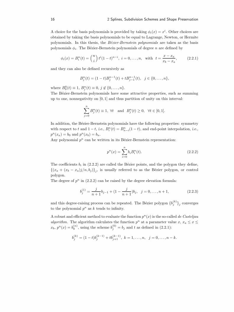
A choice for the basis polynomials is provided by taking φi(x) = xi. Other choices areobtained by taking the basis polynomials to be equal to Lagrange, Newton, or Hermitepolynomials. In this thesis, the Bezier-Bernstein polynomials are taken as the basispolynomials φi. The Bezier-Bernstein polynomials of degree n are defined by
φi(x) = Bni (t) =(ni
)ti(1− t)n−i, i = 0, . . . , n, with t =
x− xaxb − xa
, (2.2.1)
and they can also be defined recursively as
Bnj (t) = (1− t)Bn−1j (t) + tBn−1
j−1 (t), j ∈ 0, . . . , n,
where B00(t) ≡ 1, Bnj (t) ≡ 0, j 6∈ 0, . . . , n.
The Bezier-Bernstein polynomials have some attractive properties, such as summingup to one, nonnegativity on [0, 1] and thus partition of unity on this interval:
n∑j=0
Bnj (t) ≡ 1, ∀t and Bnj (t) ≥ 0, ∀t ∈ [0, 1].
In addition, the Bezier-Bernstein polynomials have the following properties: symmetrywith respect to t and 1− t, i.e., Bni (t) = Bnn−i(1− t), and end-point interpolation, i.e.,pn(xa) = b0 and pn(xb) = bn.Any polynomial pn can be written in its Bezier-Bernstein representation:
pn(x) =n∑i=0
biBni (t). (2.2.2)
The coefficients bi in (2.2.2) are called the Bezier points, and the polygon they define,(xa + (xb − xa)j/n, bj)j , is usually referred to as the Bezier polygon, or controlpolygon.The degree of pn in (2.2.2) can be raised by the degree elevation formula:
b(1)j =
j
n+ 1bj−1 + (1− j
n+ 1)bj , j = 0, . . . , n+ 1, (2.2.3)
and this degree-raising process can be repeated. The Bezier polygon b(k)j j converges
to the polynomial pn as k tends to infinity.
A robust and efficient method to evaluate the function pn(x) is the so-called de Casteljaualgorithm. The algorithm calculates the function pn at a parameter value x, xa ≤ x ≤xb, pn(x) = b
(n)0 , using the scheme b(0)
j = bj and t as defined in (2.2.1):
b(k)j = (1− t)b(k−1)
j + tb(k−1)j+1 , k = 1, . . . , n, j = 0, . . . , n− k.

2.2 Splines 17
The calculation scheme from de Casteljau takes repeated linear combinations of Bezierpoints, which finally produces the function value at the local parameter t: pn(t) = b
(n)0 .
Splines. A spline is defined by a collection of piecewise connected analytic functions,e.g., polynomials pni (x), on every subinterval separately instead of one single analyticfunction on the entire interval. The motivation to introduce a spline is to keep thesmoothness and to increase the flexibility. Another reason of using a spline insteadof e.g., polynomials, is to reduce oscillations, i.e., shape preservation. In case of poly-nomial basis functions, the collection of piecewise polynomials is called a polynomialspline, or briefly a spline.Consider the interval [xa, xb], which is partitioned in Nξ segments Ii := [ξi−1, ξi[,i = 1, . . . , Nξ − 1, INξ := [ξNξ−1, ξNξ ]. The knots ξj are strictly monotone increasing:ξj−1 < ξj , j = 1, . . . , Nξ, and the end-points satisfy ξ0 = xa and ξNξ = xb. On eachsubinterval Ii, one can define the polynomial pni (x) as (see (2.2.2))
pni (x) =n∑j=0
bni,jBnj (t), (2.2.4)
and the local parameter 0 ≤ t ≤ 1 is defined as
t =x− ξiξi+1 − ξi
, x ∈ [ξi, ξi+1]. (2.2.5)
The n-th degree spline u(x) is defined by a collection of polynomials:
u(x|x ∈ Ii) = pni (x), i = 1, . . . , Nξ.
Two neighbouring polynomials pni and pni+1 are not continuously differentiable at theknot ξi, in general. Smoothness at the knots can be achieved by requiring additionalconditions on the Bezier points bni,j . The condition on the spline u to be continuousat the knot ξi becomes: bni−1,n = bni,0. Similarly, conditions on bni,j that guarantee thespline to be Ck, k ≤ n, can be derived. When this process of constructing conditionswould be continued until the spline becomes Cn (the case k = n), the spline wouldreduce to a single polynomial of degree n on the whole interval [xa, xb].
B-splines. A very useful class of spline functions is provided by so-called B-splines.The n-th degree B-spline on the knot set ξi
Nξi=0 is defined as
u(x) =N−1∑i=−n
diNni (x).
The B-spline basis functions Nni (x) consist of piecewise polynomials of degree n with
local support and smoothness Cn−1, and are defined by N0i (x) = 1 if x ∈ [ξi, ξi+1] and

18 2 Splines, Subdivision Schemes and Shape Preservation
N0i (x) = 0 if x 6∈ [ξi, ξi+1], with the (numerically stable) recursion relation
Nk+1i (x) =
x− ξiξi+k − ξi
Nki (x) +
ξi+k+1 − xξi+k+1 − ξi+1
Nki+1(x), k = 0, . . . , n− 1.
Note that if adjacent knots do not coincide, i.e., ξi−1 < ξi, = 1, . . . , N , the B-spline isn− 1 times continuously differentiable.An alternative for evaluating a B-spline and its derivatives at a certain position isprovided by the de Boor-scheme, see [dB78], which can be seen as an analogue of thede Casteljau algorithm for B-splines. Besides, there exist simple algorithms for knotinsertion, calculation of derivatives and degree raising of B-splines. Furthermore, anyB-spline can be converted to its Bezier-Bernstein formulation.
Tensor-product splines. There exists a simple generalisation of univariate B-splines tothe multivariate case: tensor-product B-splines. A bivariate tensor-product B-splinefunction u is defined as follows:
u(x, y) =Nξ−1∑i=−nx
Nη−1∑j=−ny
di,jNnxi (x)Nny
j (y). (2.2.6)
The numbers nx and ny stand for the degree of the splines in the x-direction and they-direction, respectively. The quantities Nξ and Nη determine the number of knots inboth directions.
Rational splines. As they will appear to be attractive in case of preservation of shapeproperties, also rational splines are introduced in this thesis. A general way of defininga rational spline segment on the interval [ξi, ξi+1] is to introduce the basis functions
ui(x) =ci,0 + ci,1t+ ci,2t
2 + . . .+ ci,ntn
1 + ci,n+1t+ ci,n+2t2 + . . .+ ci,n+mtm, m ≥ 0,
where t is a local parameter, see (2.2.5), and n and m are the degrees of the polynomialsin the numerator and the denominator respectively. The restriction on the coefficientsci,j is that no singularities may occur in ui. The rational splines reduce to polynomialsplines if m = 0.
2.2.2 Spline interpolation
Splines have been introduced in the previous section, and we now discuss interpolationusing splines.First, we make some remarks concerning polynomial interpolation. It is well-known thatevery univariate data set containing n+1 points can be interpolated with a polynomialof degree n, and this is usually referred to as polynomial interpolation. This is a global

2.2 Splines 19
method, since a linear system of equations has to be solved. As the number of pointsincreases, the degree of the interpolating polynomial increases, which in general isaccompanied with oscillations. This unwanted behaviour yields that this method ishardly used for large n in practice.However, attractive variants are obtained when the method is adapted a little. Onelocal method is to determine an interpolating polynomial through a limited number ofpoints, e.g., a cubic polynomial function interpolating four successive data points. Themethod is to determine a polynomial ui(x) in the interval [xi, xi+1] which interpolatesthe four points (xj , fj)i+2
j=i−1. Although this defines a polynomial spline, it is easilyseen that this spline is not C1 in general.An example of a spline interpolation method that generates C1 functions is given byHermite interpolation using cubic splines:
Example 2.2.1 (Cubic Hermite spline interpolation) Consider a cubic polynomialfunction on the interval [xi, xi+1], and require that it interpolates the Hermite datapoints (xi, fi, gi) and (xi+1, fi+1, gi+1). Define the Bezier points as
b3i = fi, b3i+1 = fi +hi3gi, b3i+2 = fi+1 −
hi3gi+1, b3i+3 = fi+1, (2.2.7)
where hi = xi+1 − xi. This yields a class of C1 Hermite-interpolating cubic splines,and the spline segment ui on the interval [xi, xi+1] is explicitly given by:
ui(x) = (1− t)fi + tfi+1 − t(1− t)hi ((1− t)(∆fi − gi) + t(gi+1 −∆fi)) , (2.2.8)
where t = (x− xi)/(xi+1 − xi) is the local variable, and the forward divided difference∆fi is defined in (2.1.6).The derivatives gj can be estimated in case they are not explicitly provided. A suitablemethod for estimating the derivatives is
gj =fj+1 − fj−1
xj+1 − xj−1,
which is a central difference around xj . At the boundary points, the derivatives can beestimated by a forward or backward divided difference, see (2.1.6). ♦
It is clear that a method like this can easily be extended to higher degree basis functions:using quintic polynomials interpolating derivatives up to degree two leads to a splineinterpolation method that generates C2 functions.
B-spline interpolation. It is previously shown that spline methods for interpolationcan be constructed that possess attractive properties such as high smoothness of the

20 2 Splines, Subdivision Schemes and Shape Preservation
interpolant, and locality, see example 2.2.1. The class of B-splines provides splinesthat have the highest degree of smoothness: a B-spline of degree n is maximal Cn−1.However, a major disadvantage is that a B-spline interpolation method is not local,i.e., a set of linear equations has to be solved, and a modification in the data generallycauses global changes in the interpolating function.
Spline approximation. Instead of interpolation, approximating splines can be consid-ered. One can distinguish two different types: global methods and local methods.Global spline approximation methods are generally formulated as optimisation prob-lems. The goal of such an optimisation approach is to minimise a function that containssome measure of the distance between the spline and the given data, in order to achievea method that fits the data in a proper way. An example of such a method is least-squares approximation, where ε2, given in (2.1.11), is minimised.In contrast with B-spline interpolation which cannot be performed using a local method,several local B-spline approximation methods exist. An example is quasi-interpolation,for which linear combinations of the given data values serve as control points in thespline representation. Quasi-interpolation is not an approximation method in the clas-sical sense: the method does not minimise the error in a certain norm.An important drawback of most spline approximation methods is that there is nocontrol on the maximum error in general, i.e., it is not simple to approximate thedata within a prescribed error tolerance. In contrast with increasing the degree of thesplines, one approach to cope with this shortcoming is to introduce additional knots,see chapter 8.
2.2.3 Splines and shape preservation
In this section, we discuss several methods for shape preserving interpolation and ap-proximation. Subsequently we discuss shape conditions for Bezier polynomials andB-splines. In addition, some shape preserving rational interpolating splines are intro-duced.
Sufficient conditions for shape preservation. An interesting question arising fromspline interpolation concerns the connection between the shape of the Bezier-net andthe shape of the corresponding spline. The following theorem holds:
Theorem 2.2.2 Consider univariate splines, and let k ∈ 0, 1, 2, then:
The Bezier-net is k-convex =⇒ The spline is k-convex
This theorem only provides a sufficient condition for shape preservation of univariatesplines. The opposite of the theorem is not true. A counterexample for 2-convexity iseasily constructed using quartic splines.

2.2 Splines 21
The following question naturally arises: how do the results for shape preservationgeneralise to B-splines? In case of preservation of k-convexity for univariate B-splines,the k-th derivative of the B-spline, u(k), is determined. A sufficient condition for kconvexity of u is obtained by requiring nonnegativity of the B-spline control points ofthe B-spline u(k). Another weaker condition is obtained as follows On every interval,the B-spline u(k) can be written in the Bezier-Bernstein representation. The sufficientcondition for positivity in theorem 2.2.2 can be applied. Sufficient conditions for shapepreservation can therefore be obtained as linear inequalities in the Bezier points, whichcan be transformed into linear inequalities in the B-spline coefficients. The constructionof linear inequalities that are sufficient for shape preservation of bivariate splines isdiscussed in chapter 8.
The univariate sufficient shape conditions from theorem 2.2.2 are also valid for bivariatesplines. However, the bivariate conditions are more restrictive that the univariate are.For example, a convex Bezier-net only admits a so-called translational surface. Thecondition for positivity preservation turns out to be less restrictive, even in case oftensor-product splines. This sufficient condition is used in chapter 8, and methods forlinearisation of shape constraints for bivariate tensor-product B-splines are introduced,which lead to linear inequalities in the B-spline control points. The complexity ofe.g., convexity preservation for multivariate functions lies in the fact that the conditionsare nonlinear when d > 1.
Interpolating rational splines. Some classes of rational splines are known to be suitedfor shape-preserving interpolation. In [Sch73], basis functions are introduced that arequadratic in the numerator and linear in the denominator:
ui(t) =ci,0 + ci,1t+ ci,2t
2
1 + ci,3t. (2.2.9)
The smoothness properties of the interpolation problem with first or second derivativesat the end-points are examined. Although the class of interpolating splines is C2-continuous, the equations in the spline coefficients are nonlinear and therefore difficultto solve. However, the rational basis functions have good shape preserving properties,due to the simple form of the second derivative, see e.g., example 2.2.4 and 2.2.5.Rational splines are useful for shape preserving Hermite interpolation. First, we givean example of convexity preserving rational splines that are cubic in the numeratorand quadratic in the denominator.
Example 2.2.3 (Convex rational Hermite interpolation) Convexity preserving Her-mite interpolation using rational splines is discussed in [DG85b]. The basis functionshave degree three in the numerator and are quadratic in the denominator. The spline

22 2 Splines, Subdivision Schemes and Shape Preservation
segment ui on the interval [xi, xi+1] that interpolates function values and derivativesis written as [DG85b]:
ui(x) = (1− t)fi + tfi+1 − hi(1− t)(∆fi − gi) + t(gi+1 −∆fi)
(wi − 3) + 1/(t(1− t)) , (2.2.10)
where t is the local coordinate on the interval [xi, xi+1]: t = (xi − x)/(xi+1 − xi).It is necessary and sufficient for ui to be convex that the tension parameter wi satisfieswi ≥ 1 +Mi/mi, where Mi and mi are respectively defined by
Mi = max∆fi − gi, gi+1 −∆fi, and mi = min∆fi − gi, gi+1 −∆fi.
If the derivatives are not provided, two choices for estimating them in a monotonicitypreserving way are suggested in [DG85a]. The arithmetic mean is
gi =hi
hi−1 + hi∆fi−1 +
hi−1
hi−1 + hi∆fi, hi = xi+1 − xi, (2.2.11)
and the harmonic mean estimate, a generalisation of [But80,FB84], satisfies
1gi
=hi
hi−1 + hi
1∆fi−1
+hi−1
hi−1 + hi
1∆fi
, (2.2.12)
Both derivative estimates are easily shown to be second order accurate. The arithmeticmean can be interpreted as determining the interpolating quadratic polynomial to thedata fi−1, fi, and fi+1, and then evaluating the derivative of this polynomial at xi. ♦
A subclass of these splines has later been discussed separately in [Del89]. As in [Sch73],this class of convexity preserving splines is quadratic in the numerator and linear inthe denominator:
Example 2.2.4 (Convex rational Hermite splines) The rational function that has aquadratic numerator and a linear denominator, and that interpolates the Hermite data(xi, fi, gi) and (xi+1, fi+1, gi+1) is given in [Del89]:
ui(x) =(xi+1 − x)fi + (x− xi)fi+1
xi+1 − xi− 1
1(x−xi)(∆fi−gi) + 1
(xi+1−x)(gi+1−∆fi)
, (2.2.13)
where ∆fi is the divided difference in (2.1.6).Determination of the second derivative of this spline ui yields
u′′i (x) =2h2
i (∆fi − gi)2(gi+1 −∆fi)2
((x− xi)(∆fi − gi) + (xi+1 − x)(gi+1 −∆fi))3 ,

2.2 Splines 23
which is easily shown to be nonnegative for all x in the interval [xi, xi+1] providedthe data are convex (gi ≤ ∆fi ≤ gi+1). Hence this defines a class of C1 interpolatingrational splines that preserve convexity.This rational spline is connected to the general class in [DG85b] by taking the tensionparameter wi in (2.2.10) to be equal to
wi = 1 +Mi
mi+mi
Mi= 1 +
∆fi − gigi+1 −∆fi
+gi+1 −∆fi∆fi − gi
.
As has been observed in [Del89], this simplifies (2.2.10) to (2.2.13). ♦
The next example deals with monotonicity preserving rational splines.
Example 2.2.5 (Monotone rational Hermite splines) In [GD82], a class of C1 mono-tonicity preserving rational splines is proposed. The spline is a piecewise rationalfunction of degree two in the numerator and the denominator defined on an interval[xi, xi+1] as follows:
ui(x) =∆fifi+1t
2 + (figi+1 + fi+1gi) t(1− t) + ∆fifi(1− t)2
∆fit2 + (gi+1 + gi)t(1− t) + ∆fi(1− t)2 , (2.2.14)
where ∆fi is the divided difference in (2.1.6) and t is the local coordinate given byt = (x − xi)/(xi+1 − xi). The gj are derivatives at xj , and if the derivatives are notsupplied, they can be estimated, see [DG85a] or example 2.2.1.The derivative of the rational spline ui(x) is given by:
u′i(x) = (∆fi)2 gi + (gi+1 −∆fi)t2 + (∆fi − gi)t(2− t)(∆fi(1− t) + (gi+1 −∆i)t(1− t) + (∆fi − gi)t2 + tgi)
2 ,
and if the data are monotone (gi ≥ 0, ∆fi ≥ 0, gi+1 ≥ 0), this expression is easilyshown to be nonnegative, which means that this rational spline preserves monotonicity.In [DG83], it is shown that this class of splines is C2 when the derivatives gi are chosenas the solution of a specific (global) system of nonlinear equations. ♦
This section is finished with an example concerning convexity preserving interpolationusing polynomial splines. This example leads to a convexity preserving subdivisionscheme, which is further examined in chapter 3.
Existence of a convex interpolating cubic spline. Given is a univariate, convex dataset (xi, fi)i, which is equidistant, i.e., xi = ih. The goal is to determine conditionson the data such that convex interpolation is possible in a fixed spline space. For
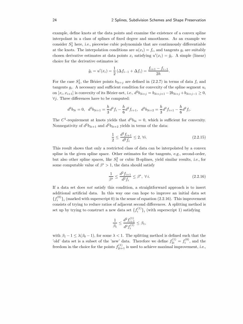
24 2 Splines, Subdivision Schemes and Shape Preservation
example, define knots at the data points and examine the existence of a convex splineinterpolant in a class of splines of fixed degree and smoothness. As an example weconsider S1
3 here, i.e., piecewise cubic polynomials that are continuously differentiableat the knots. The interpolation conditions are u(xi) = fi, and tangents gi are suitablychosen derivative estimates at data points xi satisfying u′(xi) = gi. A simple (linear)choice for the derivative estimates is:
gi = u′(xi) =12
(∆fi−1 + ∆fi) =fi+1 − fi−1
2h.
For the case S13 , the Bezier points b3i+j are defined in (2.2.7) in terms of data fi and
tangents gi. A necessary and sufficient condition for convexity of the spline segment uion [xi, xi+1] is convexity of its Bezier-net, i.e., d2b3i+j = b3i+j+1−2b3i+j+b3i+j−1 ≥ 0,∀j. Three differences have to be computed:
d2b3i = 0, d2b3i+1 =h
3d2fi −
h
6d2fi+1, d2b3i+2 =
h
3d2fi+1 −
h
6d2fi.
The C1-requirement at knots yields that d2b3i = 0, which is sufficient for convexity.Nonnegativity of d2b3i+1 and d2b3i+2 yields in terms of the data:
12≤ d2fi+1
d2fi≤ 2, ∀i. (2.2.15)
This result shows that only a restricted class of data can be interpolated by a convexspline in the given spline space. Other estimates for the tangents, e.g., second-order,but also other spline spaces, like S2
5 or cubic B-splines, yield similar results, i.e., forsome computable value of β∗ > 1, the data should satisfy
1β∗≤ d2fi+1
d2fi≤ β∗, ∀ i. (2.2.16)
If a data set does not satisfy this condition, a straightforward approach is to insertadditional artificial data. In this way one can hope to improve an initial data setf (0)i i (marked with superscript 0) in the sense of equation (2.2.16). This improvement
consists of trying to reduce ratios of adjacent second differences. A splitting method isset up by trying to construct a new data set f (1)
i i (with superscript 1) satisfying
1β1≤d2f
(1)i+1
d2f(1)i
≤ β1,
with β1− 1 ≤ λ(β0− 1), for some λ < 1. The splitting method is defined such that the’old’ data set is a subset of the ’new’ data. Therefore we define f (1)
2i = f(0)i , and the
freedom in the choice for the points f (1)2i+1 is used to achieve maximal improvement, i.e.,

2.3 Subdivision 25
try to get an β1 as small as possible. Such a splitting approach can then be repeateduntil βn < β∗, which means that convex interpolation of the data after n splitting stepsis adequate for improving the data.However, an improvement of data in the sense of ratios of adjacent second differencesis not always possible (at least in one step): take an initial data set f (0)
i i satisfying
d2f(0)2i =
√β0 and d2f
(0)2i+1 =
1√β0. (2.2.17)
This data set has the property that the ratios of adjacent second order differences aremaximal, i.e., β1 = β0, in every data point. Analytic calculations on data set (2.2.17)yield that
d2f(1)2i+1 =
12
√β0
β0 + 1=
12
1√β0 + 1√
β0
, and (2.2.18)
d2f(1)2i =
12
1√β0 (β0 + 1)
=12
1β0
1√β0 + 1√
β0
,
are optimal, and because d2f(1)2i+1/d
2f(1)2i = β0, this means that no improvement can be
achieved in one iteration, i.e., β1 = β0.The result of optimising the unknown split values f (1)
2i+1 for data set (2.2.17), whichhas been analytically derived, leads to an interesting nonlinear convexity preservingsubdivision scheme: from (2.2.18) it is easy to verify that the split points satisfy thenonlinear splitting algorithm
d2f(1)2i+1 =
12
11
d2f(0)i
+ 1d2f
(0)i+1
=⇒ f(1)2i+1 =
12
(f
(0)i + f
(0)i+1
)− 1
41
1d2f
(0)i
+ 1d2f
(0)i+1
,
It is derived in chapter 3 that this nonlinear splitting algorithm is a convexity preservingsubdivision scheme with good smoothness and approximation properties.
2.3 Subdivision
In the previous section, splines are introduced and their application to shape preser-vation is discussed. At the end of that section, a construction led to a subdivisionalgorithm. In this section, a more general treatment of subdivision schemes is pre-sented.
Given is a collection of data points f (k)i in IRd, d ≥ 1. A subdivision scheme S defines
new data f(k+1)i as f (k+1) = S(f (k)). Subdivision schemes are usually considered to
be local, i.e., they use a finite number of neighbouring points. If the scheme satisfiesf (k) = S(f (k−1)) = S(k)(f (0)), it is called stationary, which means that the same

26 2 Splines, Subdivision Schemes and Shape Preservation
subdivision rule is applied at any iteration level k, i.e., the scheme itself does notdepend on the data. Important subdivision schemes are binary schemes, which arediscrete algorithms that double the number of data in every iteration:
f(k+1)2i = F1(f (k)
i+jj),
f(k+1)2i+1 = F2(f (k)
i+jj).
A special subclass of binary schemes is obtained by looking at interpolatory subdivisionschemes, which have the property that all data at all subdivision levels remain in thedata, i.e., all data are located on the limit function:
f(k+1)2i = f
(k)i ,
f(k+1)2i+1 = F2(f (k)
i+jj).
The emphasis on subdivision schemes in this thesis is on the class (2.3), i.e., the schemesare local, binary, interpolatory, stationary and data-independent.
2.3.1 From splines to subdivision
In this section, we show a connection between splines and subdivision because splinescan also be generated in a different way, namely by subdivision. It is known thatsubdivision methods are an efficient and fast way to evaluate splines. A well-knownmethod is the De Casteljau algorithm, briefly introduced in section 2.2, which is oneof the simplest examples of an approximating subdivision scheme.
Example 2.3.1 (De Casteljau subdivision) The de Casteljau algorithm, see [dC59], istreated for the special case of quadratics, i.e., we examine a polynomial curve p2(t) ofdegree two.Let be given three points f (0)
0 , f(0)1 , f
(0)2 ∈ IR2 (the superscript (0) stands for initial
data), and define the polygon f (0) as the piecewise linear interpolant to these data.This polygon is parameterised linearly, such that f (0)(0) = f
(0)0 , f (0)(1/2) = f
(0)1 , and
f (0)(1) = f(0)2 . These three points serve as control points of the quadratic Bezier-
Bernstein polynomial p2(t) = f(0)0 (1− t)2 + 2f (0)
1 t(1− t) +f(0)2 t2, 0 ≤ t ≤ 1. This curve
p2(t) has the following properties: it is tangent to f (0) at f (0)0 and f
(0)2 . In addition,
p2(1/2) =14f
(0)0 +
12f
(0)1 +
14f
(0)2 =
12
(12
(f (0)0 + f
(0)1 ) +
12
(f (0)1 + f
(0)2 )),
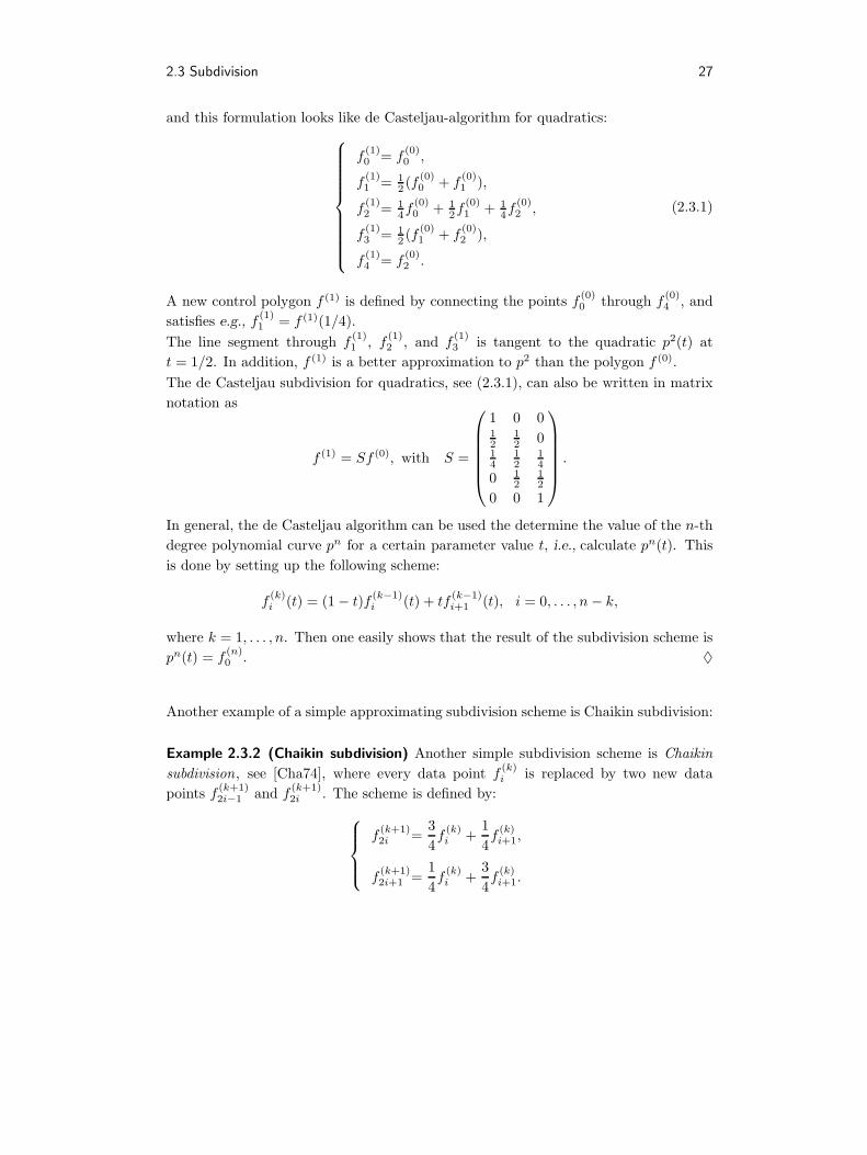
2.3 Subdivision 27
and this formulation looks like de Casteljau-algorithm for quadratics:
f(1)0 = f
(0)0 ,
f(1)1 = 1
2 (f (0)0 + f
(0)1 ),
f(1)2 = 1
4f(0)0 + 1
2f(0)1 + 1
4f(0)2 ,
f(1)3 = 1
2 (f (0)1 + f
(0)2 ),
f(1)4 = f
(0)2 .
(2.3.1)
A new control polygon f (1) is defined by connecting the points f (0)0 through f
(0)4 , and
satisfies e.g., f (1)1 = f (1)(1/4).
The line segment through f(1)1 , f (1)
2 , and f(1)3 is tangent to the quadratic p2(t) at
t = 1/2. In addition, f (1) is a better approximation to p2 than the polygon f (0).The de Casteljau subdivision for quadratics, see (2.3.1), can also be written in matrixnotation as
f (1) = Sf (0), with S =
1 0 012
12 0
14
12
14
0 12
12
0 0 1
.
In general, the de Casteljau algorithm can be used the determine the value of the n-thdegree polynomial curve pn for a certain parameter value t, i.e., calculate pn(t). Thisis done by setting up the following scheme:
f(k)i (t) = (1− t)f (k−1)
i (t) + tf(k−1)i+1 (t), i = 0, . . . , n− k,
where k = 1, . . . , n. Then one easily shows that the result of the subdivision scheme ispn(t) = f
(n)0 . ♦
Another example of a simple approximating subdivision scheme is Chaikin subdivision:
Example 2.3.2 (Chaikin subdivision) Another simple subdivision scheme is Chaikinsubdivision, see [Cha74], where every data point f (k)
i is replaced by two new datapoints f (k+1)
2i−1 and f (k+1)2i . The scheme is defined by:
f(k+1)2i =
34f
(k)i +
14f
(k)i+1,
f(k+1)2i+1 =
14f
(k)i +
34f
(k)i+1.

28 2 Splines, Subdivision Schemes and Shape Preservation
At all iterations k, a quadratic spline that interpolates the midpoints (f (k)i +f (k)
i+1)/2 canbe constructed. It is observed in [Rie75] that this approximating subdivision schemegenerates quadratic B-splines, and the subdivision matrix S reads
S =
14
34 0 0
0 34
14 0
0 14
34 0
0 0 34
14
.
The scheme is usually called a corner-cutting scheme, because of its behaviour. ♦
Similar to the Chaikin algorithm, a scheme exists that generates cubic B-splines. Thealgorithms for spline subdivision are generalised to splines of arbitrary degree overuniform knot partitions in the Lane-Riesenfeld algorithm [LR80], and for arbitraryknot sequences in the Oslo-algorithm [CLR80].
2.3.2 Approximating subdivision schemes and shape preservation
Many approximating subdivision schemes have good shape preserving properties. Anexample is e.g., the Chaikin corner cutting scheme, see section 2.3.1, which preservesconvexity. However, for many applications it is required that the error is restricted toa certain tolerance, and the approximating subdivision schemes shown above cannotguarantee this in general: e.g., the distance between the given data f (0)
i and the limitfunction f (∞) can become relatively large. This is the reason why we restrict ourselvesto interpolatory subdivision schemes in this thesis.
2.3.3 Interpolatory subdivision schemes
Probably the simplest interpolatory subdivision scheme is the two-point scheme:f
(k+1)2i = f
(k)i ,
f(k+1)2i+1 =
12
(f
(k)i + f
(k)i+1
).
(2.3.2)
This scheme is too trivial for our purposes: it generates the piecewise linear interpolantto the initial data, which is a limit function that is only C0, which is not smooth enoughfor practical applications.In [Dub86], a linear subdivision scheme based on local equidistant cubic interpolationis proposed. This scheme is extended in [DGL87] by including a tension parameter w

2.3 Subdivision 29
for shape design. This leads to the well-known linear four-point scheme:f
(k+1)2i = f
(k)i ,
f(k+1)2i+1 = −wf (k)
i−1 +(
12
+ w
)f
(k)i +
(12
+ w
)f
(k)i+1 − wf
(k)i+2,
(2.3.3)
The special case w = 1/16, for which the scheme reproduces cubic polynomials, yieldsthe scheme in [Dub86]. It is proved in [DGL87] that subdivision scheme (2.3.3) gener-ates a continuous function if the tension parameter w satisfies |w| < 1/4. The schemeconverges to C1 limit functions provided the tension parameter is restricted to therange 0 < w < 1/8. In more recent articles, convergence and smoothness is provedfor a wider range of the tension parameter, however. The approximation order of thelinear four-point scheme (2.3.3) is two, if |w| < 1/4. For w = 1/16, the scheme hasapproximation order four, see [DGL87].
Analysing the smoothness of a subdivision scheme is more difficult than determining thesmoothness of a spline. For linear subdivision schemes, however, the analysis has beenhighly developed, and some main results are summarised in section 2.4. Unfortunately,many results for linear subdivision schemes do not apply to nonlinear schemes.
2.3.4 Interpolatory subdivision and shape preservation
In this section, we discuss interpolatory subdivision schemes and their shape-preservingproperties.A simple shape-preserving subdivision scheme is the one that linearly interpolates theinitial data. This two-point scheme is defined in (2.3.2), and it is easily checked that thetwo-point scheme preserves convexity, monotonicity as well as positivity. Obviously,the two-point scheme produces a continuous curve which is not differentiable at theoriginal data points, however.The linear four-point scheme [DGL87], see (2.3.3), does not have shape-preservingproperties if it is restricted to be data-independent. For fixed values of w > 0, thescheme does not preserve convexity, monotonicity or positivity. When the tensionparameter is allowed to be data-dependent, a choice for w which only depends on theinitial data can be determined such that the shape is preserved. In [Cai95], conditionson the tension parameter w in terms of the initial data have been derived such thatmonotonicity is preserved. Although the tension parameter depends on the initial datain a nonlinear way, the construction generates a stationary interpolatory subdivisionscheme that converges to C1 limit functions which are monotone.Research in cooperation with Nira Dyn and David Levin has been done for the caseof convexity preservation of the four-point scheme, see section 2.3.5 and [D+98]. Con-ditions on the tension parameter guaranteeing preservation of convexity are derived.
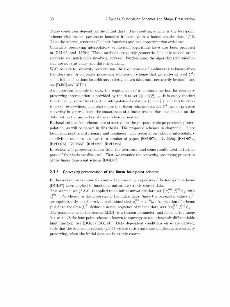
30 2 Splines, Subdivision Schemes and Shape Preservation
These conditions depend on the initial data. The resulting scheme is the four-pointscheme with tension parameter bounded from above by a bound smaller than 1/16.Thus the scheme generates C1 limit functions and has approximation order two.Convexity preserving interpolatory subdivision algorithms have also been proposedin [DLL92] and [LU94]. These methods are purely geometric, but only second orderaccurate and much more involved, however. Furthermore, the algorithms for subdivi-sion are not stationary and data-dependent.With respect to convexity preservation, the requirement of nonlinearity is known fromthe literature. A convexity preserving subdivision scheme that generates at least C1-smooth limit functions for arbitrary strictly convex data must necessarily be nonlinear,see [DJ87] and [CD94].An important example to show the requirement of a nonlinear method for convexitypreserving interpolation is provided by the data set (i, |i|)2i=−2. It is easily checkedthat the only convex function that interpolates the data is f(x) = |x|, and this functionis not C1 everywhere. This also shows that linear schemes that are C1 cannot preserveconvexity in general, since the smoothness of a linear scheme does not depend on thedata but on the properties of the subdivision matrix.Rational subdivision schemes are attractive for the purpose of shape preserving inter-polation, as will be shown in this thesis. The proposed schemes in chapter 3 – 7 arelocal, interpolatory, stationary and nonlinear. The research on rational interpolatorysubdivision schemes has lead to a number of paper: [KvD97c], [KvD98a], [KvD97a],[KvD97b], [KvD98d], [KvD98c], [KvD98b].In section 2.4, properties known from the literature, and some results used in furtherparts of the thesis are discussed. First, we examine the convexity preserving propertiesof the linear four-point scheme [DGL87].
2.3.5 Convexity preservation of the linear four-point scheme
In this section we examine the convexity preserving properties of the four-point scheme[DGL87] when applied to functional univariate strictly convex data.This scheme, see (2.3.3), is applied to an initial univariate data set (x(0)
i , f(0)i )i, with
x(0)i = ih, where h is the mesh size of the initial data. Since the parameter values x(0)
i
are equidistantly distributed, it is obtained that x(k)i = 2−kih. Application of scheme
(2.3.3) to the data f (k)i defines a nested sequence of refined data sets (x(k)
i , f(k)i )i.
The parameter w in the scheme (2.3.3) is a tension parameter, and for w in the range0 < w < 1/8 the four-point scheme is known to converge to a continuously differentiablelimit function, see [DGL87, DGL91]. Data dependent conditions on w are derived,such that the four-point scheme (2.3.3) with w satisfying these conditions, is convexitypreserving, when the initial data set is strictly convex:

2.3 Subdivision 31
Theorem 2.3.3 Given is a univariate equidistant data set (ih, f (0)i )i, which is strictly
convex. Define second order divided differences as D(k)j = 22k−1(f (k)
j−1 − 2f (k)j + f
(k)j+1),
and q(k)i and q(0) as
q(k)i =
12
D(k)i
D(k)i−1 + 2D(k)
i +D(k)i+1
, q(0) = miniq
(0)i .
Furthermore, let λ be an arbitrary real number with 1/2 < λ < 1. Then, the four pointscheme with
w = minλq(0),14λ(1− λ), λ− 1
2, (2.3.4)
preserves convexity and generates C1 limit functions.
Proof. The scheme for the second order divided differences D(k)j is given by [DGL87]:
D(k+1)2i+1 = 8w(D(k)
i +D(k)i+1),
D(k+1)2i = (2− 8w)D(k)
i − 4w(D(k)i−1 +D
(k)i+1).
It is necessary for preservation of strict convexity that D(k+1)2i+1 > 0 and D
(k+1)2i > 0,
provided D(k)i > 0. Observe that the choice of w, w > 0, shows that D(k+1)
2i+1 > 0. Next,we prove by induction that
λq(k)i ≥ w, ∀i, k, (2.3.5)
which is sufficient for convexity preservation, as λ < 1. Indeed,
D(k+1)2i = 2D(k)
i − 4w(D(k)i−1 + 2D(k)
i +D(k)i+1) = 2D(k)
i (1− w/q(k)i ) > 0.
By (2.3.4), (2.3.5) holds for k = 0. The following estimates are obtained using theinduction hypothesis and (2.3.4):
λq(k+1)2i = λ
12
D(k+1)2i
D(k+1)2i−1 + 2D(k+1)
2i +D(k+1)2i+1
=14λ− wλ
2D
(k)i−1 + 2D(k)
i +D(k)i+1
D(k)i
=14λ− λ
2λ
2w
λq(k)i
≥ 14λ− 1
4λ2 =
14λ(1− λ) ≥ w, and
λq(k+1)2i+1 = λ
2w(D(k)i +D
(k)i+1)
(1 + 2w)(D(k)i +D
(k)i+1)− 2w(D(k)
i−1 +D(k)i+2)
≥ λ2w(D(k)
i +D(k)i+1)
(1 + 2w)(D(k)i +D
(k)i+1)
= λ2w
1 + 2w≥ (w + 1/2)
2w1 + 2w
= w,
which shows that convexity is preserved.

32 2 Splines, Subdivision Schemes and Shape Preservation
The tension parameter w is bounded from above by (2.3.4), hence
14λ∗(1− λ∗) = λ∗ − 1
2=⇒ λ∗ =
12
√17− 3
2,
i.e.,
0 < w ≤ λ∗ − 12
=12
√17− 2 ≈ 0.06155 < 0.0625 =
116,
which shows that the scheme is C1 and has approximation order two, see [DGL87].
Remark 2.3.4 Depending on the initial data, the actual value of λ can easily be opti-mised such that the tension parameter w is as large as possible. Then w is closer to thevalue 1/16 for which the scheme is fourth order accurate and almost C2, see [Dub86].Furthermore, it is possible, using the above analysis, to construct non-stationary con-vexity preserving subdivision schemes by choosing w in (2.3.3) depending on k (w(k)).Indeed, it is proved in [Lev98] that the four-point scheme is C1 if w(k) is chosen ran-domly in the interval [ε, 1/8− ε] for any ε ∈]0, 1/16[. ♦
2.4 Analysis of interpolatory subdivision schemes
In this section, some definitions and fundamental results on subdivision are given. Manyresults known from the literature are based on linear subdivision schemes, and not allresults generalise to nonlinear subdivision. Overviews on subdivision can be found ine.g., [CM89, CDM91, DL90, DGL91, Dyn92, DD89, Mic95] and much of the theory andresults presented in this section has been taken from one of these papers.
Consider the initial univariate data set (x(0)i , f
(0)i )i, where x(k)
i = 2−kih, ∀k. Theschemes discussed in this thesis are restricted to the class of local, interpolatory, andstationary subdivision schemes. First a definition concerning the smoothness of subdi-vision schemes is given:
Definition 2.4.1 (Smoothness of subdivision) A stationary interpolatory subdivisionscheme is said to be C`, ` ≥ 0, if it generates limit functions f (∞) which are ` timescontinuously differentiable, and f (∞)(x(k)
i ) = f(k)i , ∀i, k.
Boundaries. A comment is made on the treatment of the boundaries. Since only localsubdivision schemes are considered, the treatment of the boundaries is not importantand does not influence the results when the following observation is taken into account:Every finite initial data set (x(0)
i , f(0)i )Ni=0 can be extended to (x(0)
i , f(0)i )N+2
i=−2, suchthat the limit function is defined everywhere inside the interval I = [x(0)
0 , x(0)N ]. For
2.4 Analysis of interpolatory subdivision schemes 33
shape preserving subdivision schemes, see the following chapters, it is assumed thatthis boundary extension is performed in some arbitrary, but shape preserving way. Bydoing so, all relevant properties on the k-th iterate in the coming chapters are easilyshown to hold for the index set Ik = 0, . . . , 2kN, or, in other words, everything willbe consistently proved on the original domain [x(0)
0 , x(0)N ] = [x(k)
0 , x(k)2kN ].
Analysis of smoothness. We briefly describe the analysis of smoothness for the subdi-vision schemes proposed in this thesis, as it has been done in the proofs of smoothnessfor the linear four-point scheme, see [DGL87]. We describe here the original approachfrom [DGL87], as it also applies to nonlinear subdivision schemes.The analysis of smoothness considers a sequence of data sets (x(k)
i , f(k)i )i. For any
iteration level k, the piecewise linear interpolating function, called f (k), is constructed.By construction, all these functions f (k) are continuous, and the only property to showfor convergence is that the sequence f (k)k converges. Then, the limit function f (∞)
exists and is C0.It is sufficient for convergence of the sequence of functions f (k) that ‖f (k+1)−f (k)‖∞ isa Cauchy sequence with limit zero. For many subdivision schemes, e.g., the linear four-point scheme, as well as many nonlinear schemes discussed in this thesis, the followingestimate can be obtained:
‖f (k+1) − f (k)‖∞ ≤ C0 maxi|f (k)i+1 − f
(k)i | = C0 max
i|df (k)
i |, C0 <∞.
The contractivity of the quantity maxi|df (k)
i | is therefore sufficient for ‖f (k+1)−f (k)‖∞to converge to zero. If e.g.,
maxi|df (k+1)
i | ≤ λ(1)df max
i|df (k)
i |, with λ(1)df < 1,
then maxi|df (k)
i | is contractive after a single iteration, which we call a single step strat-egy. However, in general contractivity cannot be proved using a single step strategy,and it is sufficient if there exists a n <∞ such that
maxi|df (k+n)
i | ≤ (λ(n)df )n max
i|df (k)
i |, with λ(n)df < 1,
which provides a n step estimate on the contractivity of the differences df (k)i .
For C1-convergence, the authors in [DGL87] consider divided differences ∆f (k)i . It
is more symmetric to attach these differences to the parameters x(k+1)2i+1 , i.e., the data
set becomes (x(k+1)2i+1 ,∆f
(k)i )i. Then at each level the piecewise linear function g(k)
that interpolates these data is determined. The subdivision scheme is then C1 if thissequence g(k) converges. Using the proper quantities of divided differences, the limit

34 2 Splines, Subdivision Schemes and Shape Preservation
function then automatically satisfies g(∞) = f (∞)′. Thus, it is shown in [DGL87] that
‖g(k+1) − g(k)‖∞ ≤ C1 maxi|∆f (k)
i+1 −∆f (k)i | = C1 max
i|s(k)i |, C1 <∞,
where s(k)i is defined in (2.1.8). Contractivity of max
i|s(k)i | is proved in [DGL87] using
a double step strategy, i.e.,
maxi|s(k+2)i | ≤ (λ(2)
s )2 maxi|s(k)i |.
This section is continued with the presentation of general results for subdivision schemes.However, note that the theory does not always hold for nonlinear schemes. For linearinterpolatory subdivision schemes, the following theorems hold, see e.g., [DGL91]:
Theorem 2.4.2 (Polynomial reproduction) A linear subdivision scheme is C`, only ifit exact for polynomials of degree `.
Theorem 2.4.3 (C0-convergence) A linear subdivision scheme for f (k)i is convergent
if and only if the scheme for the differences df (k)i = f
(k)i+1 − f
(k)i is contractive.
Theorem 2.4.4 (C`-convergence) A linear subdivision scheme is C`, ` ≥ 0, if andonly if the subdivision scheme for the differences ∆`f
(k)i exists and converges.
Theorem 2.4.5 (Difference schemes) If a linear interpolatory subdivision scheme forf
(k)i reproduces constants, then there exists a scheme for the first divided differences
∆f (k)i .
The last theorem, for example, does not generalise to nonlinear subdivision schemes.The convex scheme given in chapter 3 is a counterexample: the second difference schemeexists and reproduces constants, but there does not exist a scheme for the third differ-ences.Although theorem 2.4.5 does not generalise to nonlinear subdivision, one can requirethat a nonlinear subdivision schemes also satisfies this condition, i.e., there must exista subdivision scheme for the divided differences. This we often require for the rationalsubdivision schemes constructed in this thesis in order to reduce the number of possiblesubdivision schemes to be investigated.
Assumption 2.4.6 (Nonlinear subdivision) A stationary nonlinear interpolatory sub-division scheme can only be C`, if:
1. the scheme for the `-th differences ∆`f(k)i exists.

2.4 Analysis of interpolatory subdivision schemes 35
2. the scheme for the `-th differences ∆`f(k)i reproduces constants, i.e., the scheme
reproduces polynomials of degree `.
3. the scheme for the `-th differences d(∆`f(k)i ) exists and it is contractive.
The approximation order of subdivision schemes is also examined, and we first observethat any subdivision scheme that preserves convexity has approximation order two:
Theorem 2.4.7 (Approximation order two) Subdivision schemes for univariate data(x(k)i , f
(k)i ) that preserve convexity are second order accurate.
Proof. Consider data (x(0)i , f
(0)i ), with x
(0)i < x
(0)i+1, and f
(0)i drawn from a convex
function f ∈ C2([0, 1]). The upper envelope f(0)U is defined as the piecewise linear
interpolant to the data points (x(0)i , f
(0)i ). On the interval Ii = [x(0)
i , x(0)i+1], the lower
envelope f (0)L is defined by the maximum of the interpolating lines through (x(0)
i−1, f(0)i−1)
and (x(0)i , f
(0)i ), respectively (x(0)
i+1, f(0)i+1) and (x(0)
i+2, f(0)i+2). It is easily checked that the
intersection point x(0)i of the lower envelope lines in the interval Ii is at
x(0)i =
12
(x
(0)i + x
(0)i+1
)+
12h
(0)i
s(0)i+1 − s
(0)i
s(0)i + s
(0)i+1
.
As the function f is C2 and convex, f is located between the upper envelope f(0)U
and the lower envelope f (0)L of the initial data. Since the subdivision scheme preserves
convexity, the same holds for all linear interpolants f (k)h and also for their limit function
f(∞)h . The distance between f and f
(∞)h in Ii is therefore bounded by the difference
between f(0)L and f
(0)U at x(0), and the following estimate has been obtained:
‖f (∞)h − f‖Ii,∞ ≤ ‖f
(0)U − f (0)
L ‖Ii,∞ ≤ ‖f(0)U (x(0)
i )− f (0)L (x(0)
i )‖Ii,∞
≤ h(0)i
11s(0)i
+ 1s(0)i+1
≤ maxih
(0)i ·max
is
(0)i = O(h2),
as both h(0)i and s
(0)i are O(h). In fact, it has been used that f (0)
L is a lower bound ofthe monotone decreasing sequence of piecewise linear functions f (k)
h .
To formulate explicit statements on the approximation order of subdivision schemes,we use the notion of stability:
Definition 2.4.8 (Stability) A subdivision scheme is said to be stable, if for perturbeddata f (0)
i to f (0)i :
|f (0)i − f (0)
i | ≤ δ, ∀i =⇒ ‖f (k) − f (k)‖∞ ≤ Ckδ, with Ck < C <∞,∀k.

36 2 Splines, Subdivision Schemes and Shape Preservation
The next theorems provide sufficient conditions for the approximation order of a subdi-vision scheme. The theorems apply to linear as well as nonlinear subdivision schemes.
Theorem 2.4.9 (Approximation order) Let a subdivision scheme be stable and let itreproduce polynomials of degree p−1, with p ≥ 1. Then, this scheme has approximationorder p.
Proof. Without loss of generality, consider the interval Ii = [x(0)i , x
(0)i+1]. It is necessary
and sufficient for approximation order p that
‖f (∞)h − f‖Ii,∞ ≤ Chp, C <∞.
This can be achieved by defining f as the (p− 1)-th degree Taylor polynomial of f atx = x
(1)2i+1, which obviously satisfies
‖f − f ‖Ii,∞ ≤ C1hp, C1 <∞.
The subdivision scheme is applied to the (perturbed) data f(0)j drawn from f at the
parameters x(0)j , j = i− `, . . . , i+ 1 + `. The stability, see definition 2.4.8, implies that
the limit function f(∞)h satisfies
‖f (∞)h − f (∞)
h ‖Ii,∞ ≤ C2hp, C2 <∞,
and since the subdivision scheme reproduces polynomials of degree p, it also holds that
‖f (∞)h − f‖Ii,∞ = 0.
This yields
‖f (∞)h − f‖Ii,∞ = ‖f (∞)
h − f (∞)h + f
(∞)h − f + f − f‖Ii,∞
≤ ‖f (∞)h − f (∞)
h ‖Ii,∞ + ‖f (∞)h − f‖Ii,∞ + ‖f − f ‖Ii,∞
≤ C2hp + 0 + C1h
p = Chp,
which is valid for all i.
Theorem 2.4.10 (Approximation order) Let a subdivision scheme be stable, and letthe approximation order after one iteration be equal to p, i.e.,
‖f (1) − f‖∞ = maxi|f (1)
2i+1 − f((i+ 1/2)h)| ≤ Chp, C <∞.
Then this scheme has approximation order p, i.e.,
‖f (∞) − f‖∞ ≤ Dhp, D <∞.

2.4 Analysis of interpolatory subdivision schemes 37
Proof. In order to facilitate the proof, we use the following notations: the operator Sis used for the (nonlinear) subdivision scheme, i.e., S(k)(f (0)) := f (k). Furthermore wewrite f (k) as the unique piecewise linear function that interpolates f at the k-th levelof iteration, i.e., f (k)
i = f(x(k)i ), ∀i.
We prove thatlimk→∞
‖f (k) − f (k)‖∞ ≤ Dhp, D <∞.
The following estimate is easily obtained:
‖f (k) − f (k)‖ ≤ ‖S(1)(f (k−1))− S(1)(f (k−1))‖+ ‖S(1)(f (k−1))− f (k)‖.
The first term on the right-hand-side can be estimated as
‖S(1)(f (k−1))− S(1)(f (k−1))‖ = ‖S(2)(f (k−2))− S(1)(f (k−1))‖≤ ‖S(2)(f (k−2))− S(2)(f (k−2))‖+ ‖S(2)(f (k−2))− S(1)(f (k−1))‖,
and continuing this process, we arrive at:
‖f (k) − f (k)‖ ≤ ‖S(k)(f (0))− S(k)(f (0))‖+k∑`=1
‖S(`)(f (k−`))− S(`−1)(f (k−`+1))‖.
The first term being identically zero, the second part is further estimated using thestability of the scheme:
‖f (k) − f (k)‖ ≤k∑`=1
C`−1 · ‖S(1)(f (k−`))− f (k−`+1)‖
≤k∑`=1
C`−1 · C ·( h
2k−`)p≤ Chp ·
k∑`=1
2(`−k)p ≤ Dhp,
which completes the proof.
This theorem also justifies the approach in this thesis to construct subdivision schemes.The classes of nonlinear subdivision schemes are often restricted by considering datadrawn from a smooth function f ∈ Cp, and then requiring that the subdivision schemesatisfies ‖f (1) − f (0)‖ = ‖S(1)(f (0))− f (0)‖ ≤ Chp, C <∞.The approximation properties of linear subdivision schemes are examined by simplyapplying theorem 2.4.9. Therefore, we first discuss the stability properties of linearsubdivision schemes.
Theorem 2.4.11 (Stability of linear subdivision) Consider a linear subdivision schemethat satisfies the sufficient condition for convergence to a continuous limit function:
∃n ∈ IN, n <∞ : ‖f (k+n) − f (k)‖∞ ≤ Cλk‖f (0)‖∞, λ < 1, C <∞, (2.4.1)

38 2 Splines, Subdivision Schemes and Shape Preservation
Then, this scheme is stable.
Proof. If f (0)i are the perturbed data, define data f (0)
i := f(0)i −f
(0)i . Then, by assump-
tion, it holds that‖f (0)‖∞ ≤ δ.
The sufficient C0-condition (2.4.1) can be applied to the data f (0)i and f
(0)i , but also
to the data f (0)i , i.e.,
‖f (k+n) − f (k)‖∞ ≤ Cλk‖f (0)‖∞ ≤ Cλkδ, λ < 1,
which finally yields
‖f (∞) − f (0)‖ ≤ C
1− n√λδ =⇒ ‖f (∞)‖ = ‖f (∞) − f (∞)‖ ≤
(1 +
C
1− n√λ
)δ,
which proves stability.
In [DGL87], it has been shown that there exists a λ < 1 and a C < ∞, such that for|w| < 1/4 the linear four-point scheme (2.3.3) satisfies:
‖f (k+1) − f (k)‖∞ ≤ Cλk1‖f (0)‖∞.
Application of theorem 2.4.11 now leads to the following result:
Corollary 2.4.12 (Stability of the linear four-point scheme) The linear four-pointscheme (2.3.3) is stable if |w| < 1/4.
Many linear subdivision schemes, e.g., the four-point scheme (2.3.3), reproduce linearfunctions. Together with the stability of these schemes, see theorem 2.4.11, this prop-erty yields that these linear schemes are second order accurate. Hence, it is obtainedfor the linear four-point scheme:
Corollary 2.4.13 The linear four-point scheme (2.3.3) with |w| < 1/4 has at least ap-proximation order two.
As the linear four-point scheme with w = 1/16 is stable, and since it reproduces cubicpolynomials then, the following corollary can be formulated using theorem 2.4.9 andtheorem 2.4.11:
Corollary 2.4.14 The linear four-point scheme (2.3.3) with w = 1/16 has approxima-tion order four.
Compare the result from corollary 2.4.14 with the original proof in [DGL87].

Chapter 3
Convexity Preserving InterpolatorySubdivision Schemes
3.1 Introduction
Subdivision is now considered as a well-established technique for interpolation of data.The property of locality of subdivision schemes is attractive in many applications,e.g., computer aided design, computer graphics and vision. Several schemes for in-terpolation of data have been proposed, from which the four-point scheme [DGL87] isprobably the best-known. However, as most subdivision schemes are linear, they gener-ally do not preserve shape properties of the data, such as convexity. A characterisationof local interpolation methods that preserve strict convexity is given in [CD94].In this chapter, we examine subdivision schemes that generate limit functions thatare at least C1-smooth for arbitrary strictly convex data. If the data are convex butnot strictly convex, we require that the schemes generate convex and continuous limitfunctions. We also demand that the methods are stationary and completely local, i.e.,they do not contain any adjustable parameter depending on the initial data.A nonlinear C1-smooth convexity preserving subdivision scheme is proposed in [DLL92],which can be generalised to a honeycomb scheme for surfaces. The approach there ispurely geometric and much more involved than existing linear schemes. Another con-vexity preserving subdivision method including tension control is discussed by [LU94].The explicit formulation of the scheme that will be presented in this chapter, and isbriefly introduced in [KvD97c], meets the capabilities of [DLL92] and [LU94] with theelegance of the linear four-point scheme [DGL87].We briefly describe the outline of this chapter. Assuming certain general properties insection 3.2, a constructive approach is used in section 3.3 to derive subdivision schemesthat preserve convexity if the data are convex. The limit function generated by these

40 3 Convexity Preserving Interpolatory Subdivision Schemes
schemes is necessarily continuous now. Additionally if the data are strictly convex,a convexity preserving subdivision scheme generating continuously differentiable limitfunctions is constructed in section 3.4. The stability and approximation properties ofthis scheme are examined in section 3.5. In section 3.6, some extensions, such as tensioncontrol and piecewise convexity preservation, are briefly discussed.
3.2 Problem definition
First, we state the problem that is examined in this chapter.
Definition 3.2.1 (Problem definition) Given is a finite bounded data set (x(0)i , f
(0)i ) ∈
IR2Ni=0, which is equidistant. Without loss of generality we consider x(0)i = ih, where
h > 0 is the mesh size. Subdivision in x is defined as x(k)i = 2−kih. The first aim is
to characterise a class of subdivision schemes in f that are interpolatory and convexitypreserving. The second goal is to restrict this class of schemes to subdivision schemesthat generate continuously differentiable limit functions provided the data admit this.
A constructive approach is used to derive convexity preserving subdivision schemes.We restrict ourselves to the following class of subdivision schemes:
f(k+1)2i = f
(k)i ,
f(k+1)2i+1 =
12
(f
(k)i + f
(k)i+1
)−F1(f (k)
i−1, f(k)i , f
(k)i+1, f
(k)i+2),
(3.2.1)
for some F1. This implies that
1. The subdivision schemes are interpolatory,
2. The subdivision schemes are local, using four points.
Alternatively, this subdivision scheme can be rewritten in the following form:f
(k+1)2i = f
(k)i ,
f(k+1)2i+1 =
12
(f
(k)i + f
(k)i+1
)−F2
(12
(f (k)i + f
(k)i+1), df (k)
i , d(k)i , d
(k)i+1
),
(3.2.2)
where F2 is another function representing the same class of subdivision schemes. Thefirst and second order differences df (k)
i and d(k)i are defined in (2.1.1) and (2.1.2).
The third condition on the subdivision scheme deals with affine invariance:
3. The subdivision scheme is invariant under addition of affine functions, i.e., if thedata (x(0)
i , f(0)i ) generate subdivision points (x(k)
i , f(k)i ), then the data (x(0)
i , f(0)i +
ax(0)i + b), with a, b ∈ IR yield subdivision points (x(k)
i , f(k)i + ax
(k)i + b).
3.2 Problem definition 41
Imposing this condition yields
f(k+1)2i+1 + ax
(k+1)2i+1 + b =
12
(f
(k)i + f
(k)i+1
)+
12a(x(k)
i + x(k)i+1) + b
−F2
(12
(f
(k)i + f
(k)i+1
)+
12a(x(k)
i + x(k)i+1) + b, df
(k)i + a(x(k)
i+1 − x(k)i ), d(k)
i , d(k)i+1
).
Two conclusions can now be drawn. By taking a = 0, it follows that the term 12 (f (k)
i +f
(k)i+1) cannot explicitly occur in F2. The case b = 0 yields that df (k)
i is not presentin F2. Therefore, condition 3 yields that subdivision scheme (3.2.2) must be of thefollowing form
f(k+1)2i = f
(k)i ,
f(k+1)2i+1 =
12
(f
(k)i + f
(k)i+1
)−F(d(k)
i , d(k)i+1).
(3.2.3)
The function F is called the subdivision function and is analysed in this chapter.Next we add some natural requirements on the subdivision scheme:
4. The function F is continuous.
5. The subdivision scheme is homogeneous of degree 1, i.e., if initial data (x(0)i , f
(0)i )
give subdivision points (x(k)i , f
(k)i ), then initial data (x(0)
i , λf(0)i ) yield points
(x(k)i , λf
(k)i ).
A direct consequence of homogeneity of the method is then that F is homogeneous.
F(λx, λy) = λF(x, y), ∀λ. (3.2.4)
Furthermore, a subdivision scheme of type (3.2.3) then necessarily reproduces linearfunctions, i.e., if f (0)
i = ax(0)i + b, then f
(k)i = ax
(k)i + b (take λ = 0 in (3.2.4)).
The final general assumption on the subdivision scheme concerns with invariance underaffine transformations of the variable x:
6. The subdivision scheme is symmetric, i.e., if the initial data (x(0)i , f
(0)i ) yield
subdivision points (x(k)i , f
(k)i ), then the data (−x(0)
i , f(0)i ) yield subdivision points
(−x(k)i , f
(k)i ).
A direct result of this symmetry is that the function F is symmetric in its two argu-ments. Since F is assumed not to depend on the variables x(k)
j , condition 6 also implies
that the scheme is invariant under affine transformations of the variables x(0)i .
In this chapter, we examine the interpolation problem stated in definition 3.2.1 bysubdivision schemes of type (3.2.3) satisfying conditions 1 to 6. In the next section,we derive necessary and sufficient conditions on F for convexity preservation of suchschemes.

42 3 Convexity Preserving Interpolatory Subdivision Schemes
3.3 Convexity preservation
Consider the class of subdivision schemes (3.2.3), satisfying conditions 1 to 6 from theprevious section. Concerning the convexity preservation of these schemes, the followingtheorem holds:
Theorem 3.3.1 (Convexity) A subdivision scheme of type (3.2.3) satisfying conditions1 to 6 from section 3.2 is convexity preserving for all convex data if and only if thesubdivision function F satisfies
0 ≤ F(x, y) ≤ 14
minx, y, ∀x, y ≥ 0. (3.3.1)
Proof. For convexity preservation of subdivision scheme (3.2.3), the second differencesd
(k)i must be nonnegative for all k. Given that d(k)
i ≥ 0, ∀i, it has to be provedthat d(k+1)
i ≥ 0, ∀i. Two different second differences, d(k+1)2i+1 and d
(k+1)2i , have to be
examined:
d(k+1)2i+1 = f
(k+1)2i+2 − 2f (k+1)
2i+1 + f(k+1)2i = 2F(d(k)
i , d(k)i+1), (3.3.2)
d(k+1)2i =
12d
(k)i −F(d(k)
i−1, d(k)i )−F(d(k)
i , d(k)i+1). (3.3.3)
For non-negativity of d(k+1)2i+1 , it is necessary that the function F is nonnegative, i.e.,
F(d(k)i , d
(k)i+1) ≥ 0, (3.3.4)
whereas (3.3.3) yields
F(d(k)i−1, d
(k)i ) + F(d(k)
i , d(k)i+1) ≤ 1
2d
(k)i . (3.3.5)
As (3.3.5) must hold for any convex data, it must also hold for initial data that sat-isfy d
(0)j−1 = d
(0)j+1,∀j. Therefore, using the symmetry of F , a necessary condition on
F(d(0)i , d
(0)i+1) for convexity preservation is
F(d(0)i−1, d
(0)i ) + F(d(0)
i , d(0)i+1) = F(d(0)
i+1, d(0)i ) + F(d(0)
i , d(0)i+1) = 2F(d(0)
i , d(0)i+1) ≤ 1
2d
(0)i ,
which yields
F(d(0)i , d
(0)i+1) ≤ 1
4d
(0)i .
Again using the symmetry of F gives
F(d(0)i , d
(0)i+1) = F(d(0)
i+1, d(0)i ) ≤ 1
4d
(0)i+1.

3.3 Convexity preservation 43
Together with (3.3.4), we can conclude
0 ≤ F(d(0)i , d
(0)i+1) ≤ 1
4mind(0)
i , d(0)i+1,
and this condition is easily checked to be sufficient for convexity preservation.
Corollary 3.3.2 Convexity condition (3.3.1) directly yields the necessary condition onF that
F(x, y) = 0 if x = 0 or y = 0, (3.3.6)
which is consistent with the homogeneity condition 5 in section 2 with λ = 0.
Remark 3.3.3 Observe that the function F must be necessarily nonlinear for convex-ity preservation and C1-smoothness of subdivision scheme (3.2.3): the only (bi-)linearscheme that preserves convexity is given by F ≡ 0. However, the resulting two-pointsubdivision scheme generates the piecewise linear interpolant as limit function, whichis obviously only C0. ♦
Remark 3.3.4 A similar analysis is used to obtain the following necessary condition onthe function F for preservation of strict convexity:
0 < F(x, y) <14
minx, y 0 < x, y <∞. (3.3.7)
Convergence of subdivision scheme (3.2.3) to continuous limit functions is now a con-sequence of convexity preservation:
Theorem 3.3.5 (C0-convergence) Given is a convex data set (x(0)i , f
(0)i ) ∈ IR2i,
where x(0)i = ih. The k-th stage data (x(k)
i , f(k)i )i are defined at values x(k)
i = 2−kih.Repeated application of subdivision scheme (3.2.3) satisfying convexity condition (3.3.1)leads to a continuous function which is convex and interpolates the initial data points(x(0)i , f
(0)i ).
Proof. The interpolatory property of the subdivision scheme is a direct consequenceof the definition f
(k+1)2i = f
(k)i . The property of convexity preservation of the scheme
is proved in theorem 3.3.1. Hence, the continuous function f (k), defined as the linearinterpolant to the data (x(k)
i , f(k)i )i, is convex.
Convexity preservation of the subdivision scheme automatically guarantees that thelimit function f (∞) is continuous, when applying this scheme to arbitrary convex data:

44 3 Convexity Preserving Interpolatory Subdivision Schemes
the sequence f (k) is a monotone decreasing and bounded sequence of convex polygonsand therefore converges to a continuous convex function, see also [DLL92].
Remark 3.3.6 Following the same lines as in the proof in [DGL87], it can be easilyshown that ‖f (k+1) − f (k)‖∞ ≤ C2−k, where C <∞, since
‖f (k+1) − f (k)‖∞ = maxiF(d(k)
i , d(k)i+1) ≤ 1
4maxid
(k)i ,
and, also using the preservation of convexity, the second differences satisfy
d(k+1)2i+1 = 2F(d(k)
i , d(k)i+1) ≤ 2
14
mind(k)i , d
(k)i+1 ≤
12d
(k)i , and
d(k+1)2i =
12d
(k)i −F(d(k)
i−1, d(k)i )−F(d(k)
i , d(k)i+1) ≤ 1
2d
(k)i ,
which provides an alternative proof of convergence. ♦
The construction is continued in the next section by deriving conditions on F that aresufficient for convergence to C1 limit functions.
3.4 Convergence to a continuously differentiable function
In this section, it is investigated under what conditions subdivision schemes (3.2.3),satisfying conditions 1 to 6, and convexity condition (3.3.1) generate continuously dif-ferentiable limit functions. In the first part, we assume that the data are strictly convex.Later this restriction is relaxed.We first derive sufficient conditions on the function F . The construction presented herefollows the lines of the proof of smoothness of the limit curve generated by the linearfour-point subdivision scheme [DGL87], see section 2.4. For any strictly convex dataset (x(k)
i , f(k)i )i, first order differences ∆f (k)
i in the data are defined in (2.1.6), i.e.,
∆f (k)i :=
f(k)i+1 − f
(k)i
x(k)i+1 − x
(k)i
=2k
h
(f
(k)i+1 − f
(k)i
). (3.4.1)
The function g(k) is defined as the linear interpolant of the data points (x(k+1)2i+1 ,∆f
(k)i )
(which is a little more symmetric as in [DGL87]). The functions g(k) are thereforecontinuous by construction.We shall restrict the class of schemes such that the functions g(k) converge to a functiong(∞), which must be the derivative of f (∞), defined in the previous section.

3.4 Convergence to a continuously differentiable function 45
Sufficient for convergence of the sequence of functions g(k) is that they form a Cauchysequence in k. So it is sufficient that there exists a C1 < ∞ and µ < 1 (where µ maydepend on the initial data), such that
‖g(k+1) − g(k)‖∞ ≤ C1µk. (3.4.2)
By construction, the maximal distance between the functions g(k) and g(k+1) occursat a point x(k+2)
4i+1 = 2−k(i + 14 )h or x(k+2)
4i−1 = 2−k(i − 14 )h for some i. These distances
respectively satisfy
δ(k+1)4i+1 =
∣∣∣∣∆f (k+1)2i −
(14
∆f (k)i−1 +
34
∆f (k)i
)∣∣∣∣ =2k
h
∣∣∣∣14d(k)i − 2F(d(k)
i , d(k)i+1)
∣∣∣∣ ,δ
(k+1)4i−1 =
∣∣∣∣∆f (k+1)2i−1 −
(34
∆f (k)i−1 +
14
∆f (k)i
)∣∣∣∣ =2k
h
∣∣∣∣14d(k)i + 2F(d(k)
i , d(k)i+1)
∣∣∣∣ .Using convexity condition (3.3.1), this yields
‖g(k+1) − g(k)‖∞ = maxi
maxδ(k+1)4i+1 , δ
(k+1)4i−1 ≤
34
2k
hmaxid
(k)i . (3.4.3)
It follows from (3.4.2) and (3.4.3) that it is sufficient if maxid
(k)i can be bounded by
maxid
(k)i ≤ C2
(µ2
)k, where C2 <∞.
Note that µ may depend on the initial data.It is sufficient if we require
maxid
(k+1)i ≤ µ
2maxid
(k)i , (3.4.4)
for any strictly convex data. Therefore, using (3.3.2) and (3.3.3), it is must hold that
d(k+1)2i+1 = 2F(d(k)
i , d(k)i+1) ≤ µ
2maxjd
(k)j , (3.4.5)
d(k+1)2i =
12d
(k)i −F(d(k)
i−1, d(k)i )−F(d(k)
i , d(k)i+1) ≤ µ
2maxjd
(k)j . (3.4.6)
The construction is continued by deriving additional conditions on the function F . Thefirst additional condition is obtained by applying the sufficient condition (3.4.6) on datawith specific properties:
(i) Equation (3.4.6) must be valid for arbitrary strictly convex data. Therefore, thiscondition also holds for the class of initial data satisfying d(0)
j−1 = d(0)j+1 > 0,∀j,
which leads to the requirement
d(1)2i =
12d
(0)i − 2F(d(0)
i , d(0)i+1) ≤ µ
2maxd(0)
i , d(0)i+1, (3.4.7)

46 3 Convexity Preserving Interpolatory Subdivision Schemes
where the symmetry of F is used.
Now assume that d(0)i ≥ d
(0)i+1. The following equation must then hold:
12d
(0)i − 2F(d(0)
i , d(0)i+1) ≤ µ
2d
(0)i ,
which yields a lower bound on the function F :
F(d(0)i , d
(0)i+1) ≥ νd(0)
i , where ν =14
(1− µ) > 0.
Using the symmetry, F necessarily has to satisfy
F(d(0)i , d
(0)i+1) ≥ νmaxd(0)
i , d(0)i+1, =⇒ F(x, y) ≥ νmaxx, y, (3.4.8)
where ν > 0 depends on the initial data.
To continue the construction, we define ratios q(k)i and Q
(k)i of adjacent second order
differences in the data, as defined in (2.1.10).The homogeneity of F is then used to rewrite condition (3.4.8) as
F(d(k)i , d
(k)i+1) = d
(k)i F(1, Q(k)
i ) ≥ d(k)i νmax1, Q(k)
i .
In the case d(k)i+1 ≤ d
(k)i , it holds that 0 < Q
(k)i ≤ 1, and (3.4.8) reduces to
F(1, Q(k)i ) ≥ ν, 0 < Q
(k)i ≤ 1, ∀i, k. (3.4.9)
Our next assumption is that F should render ratios that are bounded as follows:
q(k+1) ≤ q(k), (3.4.10)
where q(k) is defined asq(k) := max
imaxq(k)
i , 1/q(k)i . (3.4.11)
Note that equation (3.4.9) is then automatically satisfied.Next, the consequences of assumption (3.4.10) for F are examined.
(ii) In this part of the construction, an upper bound on the function F is derived usingpreservation of strict convexity and condition (3.4.10). The necessary conditionfor preservation of strict convexity (3.3.7) can be rewritten as
F(d(k)i , d
(k)i+1) = d
(k)i F(1, Q(k)
i ) <14d
(k)i min1, Q(k)
i .
An additional condition on F is obtained for data with Q(k)i ≥ 1:
F(1, Q(k)i ) <
14.

3.4 Convergence to a continuously differentiable function 47
As the data are bounded and strictly convex, the ratios behave as Q(k)i ≤ q(k) ≤
q(0) <∞, and using the continuity of the function F , it must hold that
F(1, q(k)) ≤ ρ < 14,
for some ρ, which may depend on q(0). Equation (3.4.10) is used to obtain
F(d(k)j , d
(k)j+1) = d
(k)j F(1, q(k)
j ) ≤ d(k)j F(1, q(k)) ≤ ρd(k)
j ,
and the symmetry of F finally yields the condition
F(x, y) ≤ ρminx, y, ρ <14, (3.4.12)
which is an upper bound on the function F .
(iii) In the previous parts of the construction, it is assumed that the q(k) must remainbounded (condition (3.4.10) must hold). The function F is then restricted by alower bound (3.4.8) and an upper bound (3.4.12) as follows:
∀x, y > 0 : νmaxx, y ≤ F(x, y) ≤ ρminx, y, ν > 0, ρ <14. (3.4.13)
In this part bounds on ν and ρ are given. For this purpose, the ratios q(k+1)2i are
analysed (the ratios q(k+1)2i+1 give the same result).
Applying (3.3.2) and (3.3.3), the ratios q(k+1)2i become
q(k+1)2i =
d(k+1)2i
d(k+1)2i+1
=12d
(k)i −F(d(k)
i−1, d(k)i )−F(d(k)
i , d(k)i+1)
2F(d(k)i , d
(k)i+1)
=14d
(k)i − 2F(d(k)
i−1, d(k)i )
F(d(k)i , d
(k)i+1)
− 12.
Upper and lower bounds on q(k+1)2i are determined in terms of ν and ρ:
q(k+1)2i ≤ 1
4d
(k)i − 2νmaxd(k)
i−1, d(k)i
νmaxd(k)i , d
(k)i+1
− 12≤ 1
4d
(k)i − 2νd(k)
i
νd(k)i
− 12
=14ν− 1,
q(k+1)2i ≥ 1
4d
(k)i − 2ρmind(k)
i−1, d(k)i
ρmind(k)i , d
(k)i+1
− 12≥ 1
4d
(k)i − 2ρd(k)
i
ρd(k)i
− 12
=14ρ− 1.
The requirement q(k+1) ≤ q(k) from (3.4.10) yields
14ν− 1 ≤ q(k) and
14ρ− 1 ≥ 1
q(k) .
48 3 Convexity Preserving Interpolatory Subdivision Schemes
Hence, ν and ρ must satisfy
ν ≥ 14
11 + q(k) and ρ ≤ 1
41
1 + 1q(k)
=14
q(k)
1 + q(k) .
Since we assume that q(k+1) ≤ q(k), it also holds that
ν ≥ 14
11 + q(0) and ρ ≤ 1
4q(0)
1 + q(0) . (3.4.14)
Thus, the function F is necessarily restricted by
14
11 + q(0) maxx, y ≤ F(x, y) ≤ 1
4q(0)
1 + q(0) minx, y, (3.4.15)
where q(0) depends on the initial data. Note that it follows from (3.4.14) thatν > 0 and ρ < 1/4, which is consistent with (3.4.13).
(iv) It is derived in this part that the function F restricted by (3.4.15) is now deter-mined uniquely. Condition (3.4.15) must hold for the initial data:
14
11 + q(0) maxd(0)
i , d(0)i+1 ≤ F(d(0)
i , d(0)i+1) ≤ 1
4q(0)
1 + q(0) mind(0)i , d
(0)i+1.
It is known from the definition of q(k) in (3.4.10), that there exists a j for whichd
(0)j = q(0)d
(0)j+1. Substituting q(0) = d
(0)j /d
(0)j+1 in (3.4.15) then gives
14
11d
(0)j
+ 1d
(0)j+1
≤ F(d(0)j , d
(0)j+1) ≤ 1
41
1d
(0)j
+ 1d
(0)j+1
.
Therefore, F is uniquely determined and given by:
F(x, y) =14
11x + 1
y
. (3.4.16)
Remark 3.4.1 (Uniqueness) Under the restriction of adopting a single step strategy,see section 2.4, i.e., the quantity in (3.4.2) converges geometrically to zero and as-sumption (3.4.10) holds, this leads to a unique subdivision scheme. The reason of thisrestriction in the construction is the following: Since the function F is nonlinear and atwo step strategy to determine F becomes extremely difficult, it seems to be impossibleto construct all subdivision schemes that generate C1 limit functions. ♦
One unique subdivision scheme is constructed so far, which possibly generates C1-smooth limit functions if the initial data are strictly convex. We shall prove thatsubdivision scheme (3.2.3) with (3.4.16) satisfies conditions (3.4.5) and (3.4.6), i.e.,application of this scheme indeed leads to convex C1 limit functions.

3.4 Convergence to a continuously differentiable function 49
Theorem 3.4.2 (C1-convergence) Let the same conditions hold as in Theorem 3.3.5,and, in addition, let the data set (x(0)
i , f(0)i )i be strictly convex. Consider the subdi-
vision scheme of type (3.2.3) where F satisfies (3.4.16), i.e., the scheme given byf
(k+1)2i = f
(k)i ,
f(k+1)2i+1 =
12
(f
(k)i + f
(k)i+1
)− 1
41
1d
(k)i
+ 1d
(k)i+1
,(3.4.17)
with d(k)j = f
(k)j+1−2f (k)
j +f(k)j−1. Repeated application of this scheme leads to a continu-
ously differentiable function which is convex and interpolates the data points (x(0)i , f
(0)i ).
Proof. Repeating part (iii) of the construction with the specific F given in (3.4.16)immediately gives that q(k+1) ≤ q(k), where q(k) is defined in (3.4.11). Therefore
14
11 + q(0) maxd(k)
i , d(k)i+1 ≤ F(d(k)
i , d(k)i+1) ≤ 1
4q(0)
1 + q(0) mind(k)i , d
(k)i+1.
Then
d(k+1)2i+1 = 2F(d(k)
i , d(k)i+1) ≤ 2
14
q(0)
1 + q(0) mind(k)i , d
(k)i+1 ≤
12
q(0)
1 + q(0) maxjd
(k)j , and
d(k+1)2i =
12d
(k)i −F(d(k)
i−1, d(k)i )−F(d(k)
i , d(k)i+1),
≤ 12d
(k)i −
14
11 + q(0) maxd(k)
i−1, d(k)i −
14
11 + q(0) maxd(k)
i , d(k)i+1
≤ 12d
(k)i − 2
14
11 + q(0) d
(k)i =
12
q(0)
1 + q(0) d(k)i ≤ 1
2q(0)
1 + q(0) maxjd
(k)j ,
which gives
maxid
(k+1)i ≤ 1
2q(0)
1 + q(0) maxid
(k)i .
The result of (3.4.3) is
‖g(k+1) − g(k)‖∞ ≤34
2k maxid
(k)i ≤ 3
42k(
12
q(0)
1 + q(0)
)kmaxid
(0)i
=34
(q(0)
1 + q(0)
)kmaxid
(0)i ,
which proves convergence of the functions g(k) to a continuous function g(∞), as
q(0)
1 + q(0) < 1.

50 3 Convexity Preserving Interpolatory Subdivision Schemes
The remaining part of the proof is to show that also g(∞) = f (∞)′, i.e., g(k) convergesto the derivative of the limit function f (∞). This can be done by the standard ap-proach using the uniform convergence of Bernstein polynomials: the derivative of theBernstein polynomial determined by the data f (k)
i i on the interval [x(0)0 , x
(0)N ] is the
Bernstein polynomial of the data ∆f (k)i i on the same interval. This is completely
described in [DGL87]. The limit derivative g(∞) is C0, so the limit function f (∞) isC1, which completes the proof.
So far, the analysis for C1-convergence is only valid for strictly convex data. If thedata are convex but not strictly convex, it can simply be shown that the subdivisionscheme does not generate a C1 limit function if the initial data are defined by f (0)
i = |i|.Indeed, there does not even exist a convex C1-smooth interpolating function in thiscase. In the following theorem, we prove that this example represents the only classof data for which the subdivision scheme will not generate continuously differentiablelimit functions.
Theorem 3.4.3 Repeated application of subdivision scheme (3.4.17) to the convex ini-tial data set (x(0)
i , f(0)i )i generates a convex limit function which is continuously dif-
ferentiable if and only if the following condition on the initial data holds
@ j such that d(0)j > 0 and d
(0)j−1 = d
(0)j+1 = 0, (3.4.18)
where d(0)i = f
(0)i+1 − 2f (0)
i + f(0)i−1.
Proof. We first remark that a dataset for which (3.4.18) does not hold, does not admita convex and continuously differentiable interpolant. Now we show that if (3.4.18)holds, the subdivision scheme will render a C1-smooth limit function.Therefore, consider a dataset for which (3.4.18) holds. First, the smoothness of thesubdivision scheme is proved between two adjacent data points of the initial data set.In the second part of the proof the smoothness of the limit function in the initial datapoints is examined.
(i) Without loss of generality, consider the interval between x(0)0 and x
(0)1 . First
consider the case that d(0)0 = 0 or d(0)
1 = 0. This yields that the limit functionbecomes linear in the interval [x(0)
0 , x(0)1 ], and thus C1 in the interval ]x(0)
0 , x(0)1 [.
Next assume that both differences are strictly positive, i.e., d(0)0 , d
(0)1 > 0. This
yields that all second differences from d(k)0 to d
(k)2k are strictly positive for all
k. The limit function is then C1 in the interior of the interval, as shown intheorem 3.4.2.
3.4 Convergence to a continuously differentiable function 51
(ii) In this part the smoothness of the limit function is examined in the initial datapoints. Without loss of generality, consider the point (x(0)
0 , f(0)0 ) (this can be
achieved by a shift). At any subdivision level k, the limit function in the neigh-bourhood of x(0)
0 is determined by the data points f (k)−2 , f (k)
−1 , f (k)0 , f (k)
1 , and f (k)2 .
It is clear from section 3.2 that the three second differences d(k)−1 , d(k)
0 , and d(k)1
control the smoothness of the limit function in x(0)0 .
Without loss of generality, the non-trivial case is when d(0)−1 = 0 and d
(0)0 > 0,
and d(0)1 ≥ 0 holds. Therefore define the (convex) data set f (0)
−2 = 0, f (0)−1 = 0,
f(0)0 = 0, f (0)
1 = d(0)0 > 0 and f (0)
2 = f(0)0 + 2f (0)
1 +d(0)1 = 2d(0)
0 +d(0)1 . Application
of subdivision scheme (3.4.17) yields that f (k)−2 = f
(k)−1 = f
(k)0 = 0 for all k, and
that f (k)1 and f (k)
2 satisfyf
(k+1)2 = f
(k)1 = d
(k)0 ,
f(k+1)1 =
12
(f
(k)0 + f
(k)1
)−F(d(k)
0 , d(k)1 ) =
14d
(k)0
2d(k)0 + d
(k)1
d(k)0 + d
(k)1
,
from which it can be derived that
d(k+1)0 =
14d
(k)0
2d(k)0 + d
(k)1
d(k)0 + d
(k)1
and d(k+1)1 =
12
d(k)0 d
(k)1
d(k)0 + d
(k)1
.
The solution of these recursive equations is given byd
(k)0 = 2−k
d(0)0 (2d(0)
0 + d(0)1 )
2d(0)0 + (1 + k)d(0)
1
, and
d(k)1 = 2−k
d(0)1 (2d(0)
0 + d(0)1 )(
2d(0)0 + (1 + k)d(0)
1
)(d
(0)0 + 1
2kd(0)1
) .Necessary and sufficient for C1-smoothness in x(0)
0 is that the derivative from theright is equal to the derivative from the left, i.e.,
limk→∞
∆f (k)0 = lim
k→∞∆f (k)−1 , (3.4.19)
where ∆f (k)i are defined in (3.4.1). As ∆f (k)
−1 = 0,∀k, and
∆f (k)0 = 2kf (k)
1 = 2kd(k)0 =
d(0)0 (2d(0)
0 + d(0)1 )
2d(0)0 + (1 + k)d(0)
1
,
and this yields that if and only if d(0)1 > 0
limk→∞
∆f (k)0 = lim
k→∞
d(0)0 (2d(0)
0 + d(0)1 )
2d(0)0 + (1 + k)d(0)
1
= 0 = limk→∞
∆f (k)−1 ,

52 3 Convexity Preserving Interpolatory Subdivision Schemes
which proves (3.4.19).
The results of (i) and (ii) complete the proof of theorem 3.4.3.
Remark 3.4.4 Note that (3.4.18) is also the right characterisation for interpolation ofa convex data set by any convex C1 function. Any convex data admit a C1 convexlimit function if and only if condition (3.4.18) holds. ♦
A numerical example shows the performance of the subdivision scheme applied to theinitial data (x(0)
i , f(0)i )i, with x
(0)i = i and f (0)
i = |i− 1/2|.
−3 −2 −1 0 1 2 3 4−1.5
−1
−0.5
0
0.5
1
1.5
f (∞)
x −3 −2 −1 0 1 2 3 4−1.5
−1
−0.5
0
0.5
1
1.5
f (∞)
x
Figure 3.1: The first derivatives of the limit functions obtained by the linear four-pointscheme and the convex scheme for data f (0)
i = |i− 1/2|.
Figure 3.1 displays the first derivative of the limit function. The first plot is generatedby repeated application of the linear four-point scheme [DGL87] with w = 1/16, wherethe second plot is obtained by the convexity preserving scheme (3.4.17). Since bothschemes are local and reproduce linear functions, the limit functions only differ in theinterval [−2, 3]. Since the derivative in the left plot is not monotone increasing, thisexample shows that the linear four-point scheme does not preserve convexity in general.Convergence of the convexity preserving subdivision scheme to convex and continuouslydifferentiable limit functions is illustrated in the second figure by a derivative that iscontinuous and monotone increasing.
3.5 Stability and Approximation order 53
3.5 Stability and Approximation order
In this section we first examine stability properties of convexity preserving subdivi-sion schemes. It turns out that under weak conditions such schemes are always stable.Henceforth, due to theorem 2.4.10 the approximation properties of the convexity pre-serving subdivision scheme (3.4.17) can easily be obtained. A simple calculation showsthat the scheme reproduces quadratic polynomials, which suggests third order accuracy.However, the scheme has approximation order four.
Theorem 3.5.1 (Stability) Let F : IR+ × IR+ → IR be C1 and homogeneous of degree1 in its arguments. Then interpolatory subdivision schemes in the class (3.2.3) whichsatisfy condition (3.3.1) and the condition that there exist 0 < α ≤ β <∞ such that
α ≤ maxi
maxd(k)i /d
(k)i+1, d
(k)i+1/d
(k)i ≤ β, ∀k,
are stable.
Proof. Let the initial data satisfy
maxi|f (0)i − f (0)
i | ≤ δ. =⇒ maxi|d(0)i − d
(0)i | ≤ 4δ.
We have to prove that
maxi|f (k)i − f (k)
i | ≤ Ckδ, Ck <∞ and limk→∞
Ck <∞.
We give a proof by induction, and therefore we assume that
maxi|f (k)i − f (k)
i | ≤ Ckδ.
Consider the difference ‖f (k+1) − f (k+1)‖, which satisfies the estimate:
‖f (k+1) − f (k+1)‖∞ = ‖f (k+1) − f (k) + f (k) − f (k) + f (k) − f (k+1)‖∞≤ ‖f (k) − f (k)‖∞ + ‖f (k+1) − f (k) + f (k) − f (k+1)‖∞,
and substitution of the definitions yields
‖f (k+1) − f (k+1)‖∞ ≤ ‖f (k) − f (k)‖∞ + maxi|F(d(k)
i , d(k)i+1)−F(d(k)
i , d(k)i+1)|.
Making a Taylor series around (d(k)i , d
(k)i+1) yields
F(d(k)i , d
(k)i+1) = F(d(k)
i , d(k)i+1) + F1
(τd
(k)i + (1− τ)d(k)
i , τd(k)i+1 + (1− τ)d(k)
i+1
)· |d(k)
i − d(k)i |+ F2
(τd
(k)i + (1− τ)d(k)
i , τd(k)i+1 + (1− τ)d(k)
i+1
)· |d(k)
i+1 − d(k)i+1|
54 3 Convexity Preserving Interpolatory Subdivision Schemes
for some 0 ≤ τ ≤ 1, where Fj denotes the partial derivative of F with respect to itsj-th argument.Convexity preservation demands the inequality (3.3.1), but as ratios of second differ-ences are assumed to be bounded with a certain α and β (possibly depending on theinitial data) we can easily show that there must exist a ρ < 1 such that
F(x, y) ≤ ρ
4min(x, y).
By applying the identity of Euler for homogeneous functions of degree 1:
F(x, y) = F1(x, y)x+ F2(x, y)y,
we can get the following estimate. Assume x ≤ y, then
F1(x, y)x+ F2(x, y)x ≤ F1(x, y)x+ F2(x, y)y = F(x, y) ≤ ρ
4min(x, y) ≤ ρ
4x,
which proves 0 ≤ F1(x, y) + F2(x, y) ≤ ρ/4. The case x ≥ y can be treated similarly.This yields∣∣∣F(d(k)
i , d(k)i+1)−F(d(k)
i , d(k)i+1)
∣∣∣≤ max
i
∣∣∣d(k)i − d
(k)i
∣∣∣ · max0≤τ≤1
(F1
(τd
(k)i + (1− τ)d(k)
i , τd(k)i+1 + (1− τ)d(k)
i+1
)+ F2
(τd
(k)i + (1− τ)d(k)
i , τd(k)i+1 + (1− τ)d(k)
i+1
))≤ ρ
4maxi
∣∣∣d(k)i − d
(k)i
∣∣∣ .We continue with∣∣∣d(k+1)
2i+1 − d(k+1)2i+1
∣∣∣ = 2∣∣∣F(d(k)
i , d(k)i+1)−F(d(k)
i , d(k)i+1)
∣∣∣ ≤ ρ
2
∣∣∣d(k)i − d
(k)i
∣∣∣ and∣∣∣d(k+1)2i − d(k+1)
2i
∣∣∣ ≤ 12
∣∣∣d(k)i − d
(k)i
∣∣∣+∣∣∣F(d(k)
i−1, d(k)i )−F(d(k)
i−1, d(k)i )∣∣∣
+∣∣∣F(d(k)
i , d(k)i+1)−F(d(k)
i , d(k)i+1)
∣∣∣≤(
12
+ 2ρ
4
)maxi
∣∣∣d(k)i − d
(k)i
∣∣∣ =: µmaxi
∣∣∣d(k)i − d
(k)i
∣∣∣ , µ < 1.
This yields maxi|d(k)i − d
(k)i | ≤ 4δµk, and the conclusion is
‖f (k+1) − f (k+1)‖∞ ≤ ‖f (k) − f (k)‖∞ +Aµk.
Therefore Ck+1 ≤ Ck+Aµk, with µ < 1, which yields that Ck is a bounded sequence.
Remark 3.5.2 Note that the proof essentially uses the locality of four points. How-ever, if one considers less local methods which are C2, one can easily prove that suchsubdivision schemes are also stable. ♦
3.5 Stability and Approximation order 55
As any convexity preserving scheme must necessarily reproduce linear functions, thestability of the subdivision scheme (3.2.3) with (3.4.16) is sufficient for second orderaccuracy of convexity preserving interpolatory subdivision schemes, so the stabilityproof gives an alternative proof of theorem 2.4.7.Using Taylor’s theorem on initial data drawn from a sufficiently smooth strictly convexfunction, and application of theorem 2.4.10, one gets:
Corollary 3.5.3 The approximation order of subdivision scheme (3.4.16) equals four.
Remark 3.5.4 Observe that this result is only valid for strongly convex data, i.e., datadrawn from a function f with f ′′(x) > 0. Numerical experiments show that if thefunction f is C4 and convex but not strictly convex, the approximation order is alsoequal to 4. ♦
The approximation order can also be obtained by comparing the convex scheme (3.4.16)with the linear four-point scheme [DGL87] with w = 1/16, see (2.3.3). This is doneusing the following lemma (proofs can be found in [KvD98a]):
Lemma 3.5.5 Consider the data set (x(0)i , f
(0)i )Ni=0 drawn from a strongly convex
function f ∈ C4(I), where I = [x(0)0 , x
(0)N ], such that
f(0)i = f(x(0)
i ), where x(0)i = ih, and Nh = 1.
Furthermore let the functions F and F be defined as in (3.4.16) and
F(x, y) =18
(x+ y). (3.5.1)
The second differences d(k)j and d(k)
j are obtained by repeated application of subdivisionscheme (3.2.3) and (3.5.1), respectively.Then, the following statements hold:
maxi|F(d(k)
i , d(k)i+1)− F(d(k)
i , d(k)i+1)| ≤ B2−kh4,
maxi|F(d(k)
i , d(k)i+1)− F(d(k)
i , d(k)i+1)| ≤ 3
2B2−kh4,
where B is defined by
B =132
maxxf ′′(x) ·max
x
(f ′′′(x)f ′′(x)
)2.

56 3 Convexity Preserving Interpolatory Subdivision Schemes
Since the linear four point scheme is fourth order accurate, there exists a C <∞ suchthat ‖f (∞
h )− g‖ ≤ Ch4. Then, it can be obtained that
‖f (∞h )− f‖∞ ≤ ‖f (∞
h )− f (∞h ‖∞ + ‖f (∞
h − f‖∞ ≤ (5B + C)h4,
i.e., the convexity preserving subdivision scheme has approximation order four.
3.6 Generalisations
In this section, some generalisations are briefly discussed. First the subdivision schemeis extended with a tension parameter. Furthermore, the scheme is generalised to thecase of piecewise convex data, i.e., data with convex and concave intervals. It is shownthat such a piecewise convexity preserving subdivision scheme also generates contin-uously differentiable limit functions. A geometric interpretation of the subdivisionscheme is briefly given, and the relation with rational interpolation is discussed.
Shape control. Convexity preserving shape control seems to be impossible, since wehave constructed only one subdivision scheme in section 3.4. However, note that mostshape effects on the limit function are achieved by the first few subdivisions. A proce-dure to incorporate shape control can be as follows.
1. The first k∗ iterations, controlling the shape of the limit function, are performedby a subdivision scheme that only preserves strict convexity. Repeated applicationof such a scheme need not necessarily lead to C1 limit functions.
2. Smoothness of the limit function is achieved by application of subdivision scheme(3.4.17) for the final iterations, k∗ + 1 . . .∞. Since strict convexity is preservedduring the initial subdivisions, convergence to a C1 function is still guaranteed.
This process shows that it is useful to briefly examine subdivision schemes that donot generate C1 limit functions, but that do preserve strict convexity. For example,subdivision scheme (3.4.17) can be extended with a tension parameter w as follows
f(k+1)2i+1 =
12
(f
(k)i + f
(k)i+1
)− w
41
1d
(k)i
+ 1d
(k)i+1
. (3.6.1)
An admissible range on the tension parameter for preservation of strict convexity is0 < w ≤ 1. Note that this subdivision scheme coincides with (3.4.17) for w = 1, andthat the scheme converges to the piecewise linear interpolant as the tension parametertends to 0. The approximation order decreases to 2 if w 6= 1.Local shape control is obtained by replacing the tension parameter w in (3.6.1) by alocal tension parameter w(k)
i assigned to each data point individually.

3.6 Generalisations 57
Piecewise convexity. Subdivision scheme (3.4.17) can be generalised to a piecewiseconvexity preserving subdivision scheme that is capable of interpolating general (non-convex) data, such that the limit function is piecewise convex and concave and contin-uously differentiable. This is for example achieved by the scheme
f(k+1)2i+1 =
12
(f
(k)i + f
(k)i+1
)− 1
41
1d
(k)i
+ 1d
(k)i+1
, if d(k)i d
(k)i+1 > 0,
12
(f
(k)i + f
(k)i+1
), if d
(k)i d
(k)i+1 ≤ 0,
(3.6.2)
or, briefly, subdivision scheme (3.2.3) with FPC(x, y) = F(max0, x,max0, y),where F is given in (3.4.16). Note that this scheme can be applied to arbitrary data,and that it reduces to (3.4.17) if the data are convex (or concave).
The behaviour of subdivision scheme (3.6.2) differs in the inflection regions separatingconvex and concave parts in the data. An interval [x(0)
j , x(0)j+1] for some j is called
an inflection region if d(0)j d
(0)j+1 < 0. The limit function generated by the subdivision
scheme becomes linear in inflection regions.
The approximation order of the piecewise convexity preserving subdivision scheme willbe lower than four, because of the behaviour in the inflection regions where the dataare no longer strictly convex, see section 3.5. A straightforward analysis shows that thenumber of data points where the second differences change sign does not increase withthe subdivision level k. For this reason, the approximation order in L∞-norm reducesto 3 (and not to 2, since in the inflection regions g′′(x) = O(h)), the approximationorder in the L2-norm reduces to 3 1
2 .
Using the proof of theorem 3.4.3, it can be proved that subdivision scheme (3.6.2)generates continuously differentiable limit functions if and only if there does not exist aj such that d(0)
j 6= 0, d(0)j−1d
(0)j ≤ 0 and d(0)
j d(0)j+1 ≤ 0, i.e., the initial data do not contain
two adjacent inflection regions.
Smoother results are obtained if the linear four-point scheme is used instead of thetwo-point scheme when d
(k)i d
(k)i+1 < 0. However, the analysis of smoothness is then
more difficult, since the inflection point can move in the inflection interval and its limitlocation depends on the data.
A geometric interpretation. Subdivision scheme (3.4.17) has a relatively simple geo-metric interpretation in terms of reciprocals of second divided differences:
1
∆2f(k+1)2i+1
=12
(1
∆2f(k)i
+1
∆2f(k)i+1
). (3.6.3)
58 3 Convexity Preserving Interpolatory Subdivision Schemes
Compare this result with the geometric interpretation of the linear four-point schemewith w = 1/16, which satisfies:
∆2f(k+1)2i+1 =
12
(∆2f
(k)i + ∆2f
(k)i+1
),
i.e., the linear four-point scheme linearly weights second differences, whereas the con-vexity preserving scheme averages reciprocals of second differences.
Bivariate subdivision. Our research on bivariate shape preserving subdivision dealswith convexity preserving subdivision for triangulations. A butterfly-like scheme basedon six neighbouring triangles is proposed in [DLL92]. Second differences, based on fourpairs of adjacent triangles, are there weighted linearly, whereas we propose to weightthem harmonically, see (3.6.3). This leads to bivariate functions for which we canonly prove convergence. A combination of the numerical approach in chapter 6 maybeprovides a methodology to construct and to prove convergence to C1 functions in thebivariate case.
Connection with rational interpolation. It can easily be verified that subdivisionscheme (3.4.17) reproduces quadratic polynomials, and in [FM98] it is shown to repro-duce rational functions that are quadratic in the numerator and linear in the denomina-tor. This class of rational functions has been introduced in [Sch73] as a basis functionin a class of rational splines, see (2.2.9). Although that class of interpolating splinesis C2-continuous, the equations in the spline coefficients are nonlinear and thereforedifficult to solve.The rational function ui(x) of this form that interpolates the data (xj , fj)i+2
j=i−1, withxi = ih, can be written as
ui(t) = (1− t)fi + tfi+1 −32h
t(1− t)2−tsi
+ 1+tsi+1
, t =x
h, 0 ≤ t ≤ 1, (3.6.4)
where si are defined as differences of first divided differences, see (2.1.8).It is easily seen that the spline ui is (globally) convex, if the data are convex. Inaddition, the spline ui is continuously differentiable at the parameter values xi. Asis shown in chapter 5 however, these observations do not generalise to the case wherethe data xi are nonuniform.Evaluation of the function ui in (3.6.4) at t = 1/2 yields
ui (1/2) =12
(fi + fi+1)− 14h
11si
+ 1si+1
,
which defines the subdivision scheme introduced in this chapter.

Chapter 4
Monotonicity Preserving InterpolatorySubdivision Schemes
4.1 Introduction
A class of four-point nonlinear stationary subdivision schemes that preserve monotonic-ity is examined. These schemes are used for interpolation of univariate data that areequidistant and monotone increasing (or decreasing). Many schemes known from litera-ture however, fail to preserve monotonicity in the data in general. Linear monotonicitypreserving subdivision schemes are discussed in [YS93], but the schemes discussed thereare not interpolatory. Monotonicity preservation of the interpolatory linear four-pointscheme [DGL87] is discussed in [Cai95]. The author determines ranges on the tensionparameter such that the scheme is monotonicity preserving. Since the tension param-eter depends on the initial data, the resulting subdivision scheme is stationary, butdata-dependent, however.We restrict ourselves to subdivision schemes that guarantee the preservation of mono-tonicity in the data. It is stressed that there is an analogy with chapter 3, in whichconvexity preserving interpolatory subdivision schemes are examined. The same con-structive approach is used, and so there is a similarity in some of the proofs. Theremark in chapter 3 that convexity preserving interpolatory subdivision schemes gen-erating C1 limit functions must necessarily be nonlinear also holds for monotonicitypreserving schemes. The schemes examined in this chapter are stationary and they donot contain any data-dependent tension parameter.The overview of this chapter is as follows. Section 4.2 states the problem and theclass of schemes under investigation. The condition for preservation of monotonicity isderived in section 4.3, and in section 4.4 convergence to a limit function is examined.The analysis for convexity preservation in chapter 3 led to a scheme that is unique in

60 4 Monotonicity Preserving Interpolatory Subdivision Schemes
some sense, if convergence to a C1 function is required. Requiring convergence to aC1-smooth monotone function leads to a larger class of subdivision schemes however.Sufficient conditions for convergence to a C1 limit function are given in section 4.5, andsince these conditions are too complex for constructing explicit subdivision schemes,we restrict ourselves to rational subdivision schemes, see section 4.6. Section 4.7 showsthat these schemes have the property that ratios of adjacent first order differences tendto 1 as k tends to infinity. For any initial monotone data these schemes converge tocontinuously differentiable limit functions (see section 4.8). Moreover, the schemesare stable and they have approximation order four (section 4.9). Some generalisationsare briefly discussed in section 4.10: e.g., piecewise monotonicity and application tohomogeneous grid refinement which is a useful property for subdivision schemes forfunctional nonequidistant data, see chapter 5.
4.2 Problem definition
First, we state the problem that is examined in this chapter.
Definition 4.2.1 (Problem definition) Given is a data set (t(0)i , x
(0)i ) ∈ IR2Ni=0, where
the parameter values are equidistantly distributed, i.e., without loss of generality t(0)i =
i, The data are assumed to be monotone, i.e., x(0)i ≤ x
(0)i+1, ∀i, or x
(0)i ≥ x
(0)i+1, ∀i.
Subdivision in t is defined as t(k)i = 2−ki, i = 0, . . . , 2kN . The aim is to characterise a
class of subdivision schemes that are interpolatory and monotonicity preserving. Thesecond goal is to restrict this class of subdivision schemes to schemes that generatecontinuously differentiable limit functions and are fourth order accurate.
A constructive approach is used to derive monotonicity preserving subdivision schemes.Without loss of generality, we consider monotone increasing data, briefly denoted asmonotone data.We restrict ourselves to the following class of schemes:
x(k+1)2i = x
(k)i ,
x(k+1)2i+1 =
12
(x
(k)i + x
(k)i+1
)+ G1(x(k)
i−1, x(k)i , x
(k)i+1, x
(k)i+2),
(4.2.1)
for some function G1. This implies that
1. The subdivision schemes are interpolatory,
2. The subdivision schemes are local, using four points.

4.2 Problem definition 61
Subdivision scheme (4.2.1) can then be rewritten using the definition of differences h(k)i ,
see (2.1.3), in the following form:x
(k+1)2i = x
(k)i ,
x(k+1)2i+1 =
12
(x
(k)i + x
(k)i+1
)+ G2
(12
(x(k)i + x
(k)i+1), h(k)
i−1, h(k)i , h
(k)i+1
),
(4.2.2)
where G2 is another function representing the same class of subdivision schemes.The third condition on the subdivision schemes deals with invariance under additionof constants:
3. The subdivision scheme is invariant under addition of constant functions, i.e., ifdata (t(0)
i , x(0)i ) generate subdivision points (t(k)
i , x(k)i ), then data (t(0)
i , x(0)i + µ),
with µ ∈ IR yield subdivision points (t(k)i , x
(k)i + µ).
Imposing this condition yields
x(k+1)2i+1 + µ =
12
(x
(k)i + x
(k)i+1
)+ µ+ G2
(12
(x
(k)i + x
(k)i+1
)+ µ, h
(k)i−1, h
(k)i , h
(k)i+1
).
It follows that G2 cannot depend on its first argument. Condition 3 therefore yieldsthat subdivision scheme (4.2.2) must be of the following form:
x(k+1)2i = x
(k)i ,
x(k+1)2i+1 =
12
(x
(k)i + x
(k)i+1
)+ G3(h(k)
i−1, h(k)i , h
(k)i+1).
(4.2.3)
Next we add a natural requirement on the subdivision schemes:
4. The subdivision scheme is homogeneous, i.e., if initial data (t(0)i , x
(0)i ) give subdi-
vision points (t(k)i , x
(k)i ), then initial data (t(0)
i , λx(0)i ) yield points (t(k)
i , λx(k)i ).
A direct consequence of homogeneity of the subdivision schemes is that the functionG3 is homogeneous:
G3(λa, λb, λc) = λG3(a, b, c), ∀λ. (4.2.4)
Subdivision scheme (4.2.3) then necessarily reproduces constant functions, i.e., if x(0)i =
µ0, then x(k)i = µ0 (take λ = 0 in (4.2.4)).
Further simplification of the representation of subdivision scheme (4.2.3) is obtainedby using the homogeneity of G3 in (4.2.4) as follows:
G3(h(k)i−1, h
(k)i , h
(k)i+1) = h
(k)i G3(r(k)
i , 1, R(k)i+1) =
12h
(k)i G(r(k)
i , R(k)i+1),

62 4 Monotonicity Preserving Interpolatory Subdivision Schemes
where ratios of adjacent first differences r(k)i and R
(k)i are defined in (2.1.4), and the
function G is defined by G(r,R) := 2G3(r, 1, R).Since it follows in the next sections that G is a bounded function, this reformulation ofG does not cause problems in case h(k)
i = 0.The class of subdivision schemes (4.2.1) is rewritten in the form:
x(k+1)2i = x
(k)i ,
x(k+1)2i+1 =
12
(x
(k)i + x
(k)i+1
)+
12h
(k)i G(r(k)
i , R(k)i+1),
(4.2.5)
and it is this subdivision scheme that is examined in this chapter.
Remark 4.2.2 Note that the class of subdivision schemes (4.2.5) automatically satisfiesconditions 1 – 4. ♦
The next general assumption on the subdivision scheme concerns with invariance underaffine transformations of the variable t:
5. The subdivision scheme is invariant under affine transformations of the variablet, i.e., if the initial data (t(0)
i , x(0)i ) yield subdivision points (t(k)
i , x(k)i ), then the
data (λt(0)i + µ0, x
(0)i ), with µ0 ∈ IR yield subdivision points (λt(k)
i + µ0, x(k)i ) for
λ > 0, and (λt(k)i + µ0,−x(k)
i ) for λ < 0.
By taking λ = −1 and µ0 = 0 in condition 5, it follows that G is anti-symmetric underinterchanging its arguments, i.e., it is obtained that
G(r,R) = −G(R, r), ∀r,R, (4.2.6)
which directly implies G(r, r) = 0, ∀r.Under this condition on G, subdivision scheme (4.2.5) necessarily reproduces linearfunctions, i.e., if x(0)
i = λ1t(0)i +µ1, then x(k)
i = λ1t(k)i +µ1 (as h(k)
i = λ1, r(k)i = 1, ∀i).
Remark 4.2.3 Invariance under addition of linear functions is not a natural conditionin case of monotonicity preservation, in contrast with convexity preservation, see chap-ter 3. ♦
In the following sections, we discuss conditions for monotonicity preservation andsmoothness properties of subdivision scheme (4.2.5) satisfying (4.2.6), which requiresadditional conditions on the function G.

4.3 Monotonicity preservation 63
4.3 Monotonicity preservation
In this section, we examine monotonicity preservation of the class of four-point inter-polatory subdivision schemes (4.2.5) satisfying (4.2.6).
Theorem 4.3.1 (Monotonicity preservation) Subdivision scheme (4.2.5) satisfying con-dition (4.2.6) preserves monotonicity if and only if the subdivision function G satisfies
|G(r,R)| ≤ 1, ∀r,R ≥ 0. (4.3.1)
Proof. Monotonicity preservation is achieved if and only if the scheme generates dif-ferences that satisfy h(k)
i ≥ 0, ∀i, ∀k.Therefore assume that for some k, the data x
(k)i satisfy h
(k)i ≥ 0, ∀i. Necessary and
sufficient for monotonicity preservation is that the differences in the data at level (k+1)are also non-negative, i.e., h(k+1)
i ≥ 0, ∀i.Two differences, h(k+1)
2i and h(k+1)2i+1 , have to be analysed:
h(k+1)2i = x
(k+1)2i+1 − x
(k+1)2i =
12
(x
(k)i + x
(k)i+1
)+
12h
(k)i G(r(k)
i , R(k)i+1)− x(k)
i (4.3.2)
=12
(x
(k)i+1 − x
(k)i
)+
12h
(k)i G(r(k)
i , R(k)i+1) =
12h
(k)i
(1 + G(r(k)
i , R(k)i+1)
), and
h(k+1)2i+1 = x
(k+1)2i+2 − x
(k+1)2i+1 = x
(k)i+1 −
12
(x
(k)i + x
(k)i+1
)− 1
2h
(k)i G(r(k)
i , R(k)i+1) (4.3.3)
=12
(x
(k)i+1 − x
(k)i
)− 1
2h
(k)i G(r(k)
i , R(k)i+1) =
12h
(k)i
(1− G(r(k)
i , R(k)i+1)
).
Since h(k)i ≥ 0 it is necessary for monotonicity preservation that
1 + G(r(k)i , R
(k)i+1) ≥ 0 and 1− G(r(k)
i , R(k)i+1) ≥ 0,
which yields that condition (4.3.1) is sufficient for monotonicity preservation of subdi-vision scheme (4.2.5).Since we consider arbitrary monotone data, this condition is also necessary.
Remark 4.3.2 (Preservation of strict monotonicity) A sufficient condition for preser-vation of strict monotonicity is:
∃µ < 1 such that |G(r,R)| ≤ µ, ∀r,R > 0.
The two-point subdivision scheme (2.3.2), which is also called the midpoint scheme,clearly preserves monotonicity for any monotone data x(k)
i . However, it generates thepiecewise linear interpolant as limit function, which is obviously only C0.
64 4 Monotonicity Preserving Interpolatory Subdivision Schemes
Remark 4.3.3 (Nonlinearity) Observe that the function G is necessarily nonlinear formonotonicity preservation and C1-smoothness of subdivision scheme (4.2.5): the onlyscheme that is polynomial in its arguments and that satisfies (4.3.1) is given by G ≡ 0,i.e., the (C0) two-point scheme (2.3.2). ♦
Remark 4.3.4 (The linear four-point scheme) The linear four-point scheme [DGL87]with w = 1
16 is given by the function
G(r,R) =18
(r −R) . (4.3.4)
Since this function G is linear, it obviously cannot satisfy the monotonicity condi-tion (4.3.1). ♦
4.4 Convergence to a continuous function
In this section convergence of subdivision scheme (4.2.5) to continuous limit functionsis investigated. The proof follows the lines of the proof of existence and continuity ofthe limit curve generated by the linear four-point scheme in [DGL87].
Theorem 4.4.1 (C0-convergence) Given is a monotone data set (t(0)i , x
(0)i ) ∈ IR2i,
where t(0)i are equidistantly distributed, e.g., t(0)
i = i. The k-th stage data (t(k)i , x
(k)i )i
are defined at values t(k)i = 2−ki. Repeated application of subdivision scheme (4.2.5)
satisfying
∃µ < 1 such that |G(r,R)| ≤ µ, ∀r,R ≥ 0. (4.4.1)
leads to a continuous function which is monotone and interpolates the initial data points(t(0)i , x
(0)i ).
Proof. The interpolatory property of the subdivision scheme is a direct consequence ofthe definition x
(k+1)2i = x
(k)i . Preservation of monotonicity of the subdivision scheme
was shown in the previous section. Therefore, the continuous function x(k), defined asthe linear interpolant to the data (t(k)
i , x(k)i )i, is monotone.
Remains to prove that the sequence of functions x(k) converges, i.e., the limit function
x(∞) := limk→∞
x(k)
exists and is continuous.

4.5 Convergence to a continuously differentiable function 65
Sufficient for convergence is that x(k) is a Cauchy sequence in k with limit 0, i.e., itsuffices to show that
‖x(k+1) − x(k)‖∞ ≤ C0λk0 , where C0 <∞ and λ0 < 1.
The distance ‖x(k+1) − x(k)‖∞ is calculated by
‖x(k+1) − x(k)‖∞ = maxi
max∣∣∣x(k+1)
2i − x(k)i
∣∣∣ , ∣∣∣∣x(k+1)2i+1 −
12
(x
(k)i + x
(k)i+1
)∣∣∣∣ .The maximal distance between the functions x(k) and x(k+1) occurs at a point t(k+1)
2i+1 =2−k(i+ 1
2 ) for some i, which thus gives, using condition (4.3.1):
‖x(k+1) − x(k)‖∞ = maxi
∣∣∣∣x(k+1)2i+1 −
12
(x
(k)i + x
(k)i+1
)∣∣∣∣ =12
maxi
∣∣∣h(k)i G(r(k)
i , R(k)i+1)
∣∣∣≤ 1
2maxi
∣∣∣G(r(k)i , R
(k)i+1)
∣∣∣ ·maxi
∣∣∣h(k)i
∣∣∣ ≤ 12µmax
ih
(k)i . (4.4.2)
We now prove that maxih
(k)i converges to 0 as k tends to infinity. Using (4.3.2), (4.3.3)
and the monotonicity condition (4.3.1), it is obtained that
maxih
(k+1)i = max
imaxh(k+1)
2i , h(k+1)2i+1 =
12
maxi
h
(k)i
(1± G(r(k)
i , R(k)i+1)
)≤ 1
2(1 + µ) max
ih
(k)i .
Combining this result with (4.4.2) yields
‖x(k+1) − x(k)‖∞ ≤12µmax
ih
(0)i
(1 + µ
2
)k.
As µ < 1, this proves convergence of x(k), and since all functions x(k) are continuousby construction, the limit function x(∞) is continuous.
4.5 Convergence to a continuously differentiable function
In the previous sections, we derived sufficient conditions on the function G such that thesubdivision scheme preserves monotonicity and that a continuous limit function exists.An additional sufficient condition on the scheme such that it generates continuouslydifferentiable functions is presented in this section.
Theorem 4.5.1 (C1-convergence) Given is a strictly monotone data set (t(0)i , x
(0)i ) ∈
IR2i, where t(0)i = i. The k-th stage data (t(k)
i , x(k)i )i are defined at values t(k)
i =2−ki.

66 4 Monotonicity Preserving Interpolatory Subdivision Schemes
Let the function G satisfy (4.4.1) and the Lipschitz-condition
∃α > 0, ∀x, y : |G(x+ ε1, y + ε2)− G(x, y)| ≤ B1 ‖ε‖α , B1 <∞. (4.5.1)
Moreover, subdivision scheme (4.2.5) has the property that the ratios of adjacent firstorder differences, defined in (2.1.4), obey:
∃ρ < 1 : maxi
∣∣∣∣∣max
r
(k)i ,
1
r(k)i
− 1
∣∣∣∣∣ ≤ B2ρk, B2 <∞. (4.5.2)
Repeated application of such a subdivision scheme generates a continuously differen-tiable function which is monotone and interpolates the initial data points (t(0)
i , x(0)i ).
Proof. Starting from a strictly monotone data set (t(k)i , x
(k)i )i first order divided
differences ∆x(k)i in the data are defined in (2.1.5), i.e.,
∆x(k)i =
x(k)i+1 − x
(k)i
t(k)i+1 − t
(k)i
= 2kh(k)i . (4.5.3)
The function y(k) is defined as the linear interpolant of the data points (t(k+1)2i+1 ,∆x
(k)i ).
All functions y(k) are therefore continuous by construction.It has to be proved that the functions y(k) converge to a function y(∞) and then thisy(∞) will be the derivative of x(∞), defined in the previous section.Sufficient for convergence of the sequence of functions y(k) is that they form a Cauchysequence in k with limit 0, i.e., there must exist a λ1 < 1 and C1 ∈ IR such that
‖y(k+1) − y(k)‖∞ ≤ C1λ1k. (4.5.4)
By construction, the maximal distance between the functions y(k+1) and y(k) occurs ata point t(k+2)
4i+j = 2−k(i+ j4 ), for some i and j, and these distances δ(k+1)
4i+j satisfy
δ(k+1)4i+j =
∣∣∣y(k+1)(t(k+2)4i+j )− y(k)(t(k+2)
4i+j )∣∣∣ . (4.5.5)
Subsequent application of (4.5.5), (4.5.3) and the equations (4.3.2) and (4.3.3), forexample yields for the distance δ(k+1)
4i+1 :
δ(k+1)4i+1 =
∣∣∣∣∆x(k+1)2i −
(14
∆x(k)i−1 +
34
∆x(k)i
)∣∣∣∣ = 2k∣∣∣∣2h(k+1)
2i − 14h
(k)i−1 −
34h
(k)i
∣∣∣∣= 2k
∣∣∣∣14 (h(k)i − h
(k)i−1
)+ h
(k)i G(r(k)
i , R(k)i+1)
∣∣∣∣= 2kh(k)
i
∣∣∣∣14 (1− r(k)i
)+ G(r(k)
i , R(k)i+1)
∣∣∣∣

4.5 Convergence to a continuously differentiable function 67
and the other distances are determined similarly:
δ(k+1)4i = 2k
∣∣∣∣12h(k)i G(r(k)
i , R(k)i+1)− 1
2h
(k)i−1G(r(k)
i−1, R(k)i )∣∣∣∣ ,
δ(k+1)4i+1 = 2kh(k)
i
∣∣∣∣14 (1− r(k)i
)+ G(r(k)
i , R(k)i+1)
∣∣∣∣ ,δ
(k+1)4i+2 = 0,
δ(k+1)4i+3 = 2kh(k)
i
∣∣∣∣14 (1−R(k)i+1
)− G(r(k)
i , R(k)i+1)
∣∣∣∣ .The distance δ(k+1)
4i is easily estimated with
δ(k+1)4i ≤ 2k max
ih
(k)i ·max
i
∣∣∣G(r(k)i , R
(k)i+1)
∣∣∣and thus, it is obtained that
maxjδ
(k+1)j ≤ 2k max
ih
(k)i ·max
imax
∣∣∣G(r(k)i , R
(k)i+1)
∣∣∣ , ∣∣∣∣14 (1− r(k)i
)+ G(r(k)
i , R(k)i+1)
∣∣∣∣ ,∣∣∣∣14 (1−R(k)i+1
)− G(r(k)
i , R(k)i+1)
∣∣∣∣ . (4.5.6)
Subsequently, we apply assumptions (4.5.1) and (4.5.2), and also use the fact thatG(1, 1) = 0, see (4.2.6). The function G can now be estimated as follows:∣∣∣G(r(k)
i , R(k)i+1)
∣∣∣ =∣∣∣G(r(k)
i , R(k)i+1)− G(1, 1)
∣∣∣ ≤ B1
∥∥∥(r(k)i − 1, R(k)
i+1 − 1)∥∥∥α ≤ B3ρ
αk,
where B3 < ∞. According to (4.3.2) and (4.3.3), the first part of (4.5.6) can beestimated as
maxih
(k+1)i ≤ 1
2
(1 + max
i
∣∣∣G(r(k)i , R
(k)i+1)
∣∣∣)maxih
(k)i ≤ 1
2(1 +B3ρ
αk)
maxih
(k)i ,
which yields
maxih
(k)i ≤
(12
)kmaxih
(0)i
k−1∏`=0
(1 +B3ρ
α`).
Since 1 + x ≤ ex, we obtain
k−1∏`=0
(1 +B3ρ
α`)≤
k−1∏`=0
exp(B3ρ
α`)
= exp
(B3
k−1∑`=0
ρα`
)
= exp(B3
1− ραk1− ρα
)≤ exp
(B3
1− ρα)
=: B4 <∞,
and hence
maxih
(k)i ≤ B4
(12
)kmaxih
(0)i .

68 4 Monotonicity Preserving Interpolatory Subdivision Schemes
The second part of (4.5.6) is estimated as
maxi
max∣∣∣G(r(k)
i , R(k)i+1)
∣∣∣ , ∣∣∣∣14 (1− r(k)i
)+ G(r(k)
i , R(k)i+1)
∣∣∣∣ ,∣∣∣∣14 (1−R(k)i+1
)− G(r(k)
i , R(k)i+1)
∣∣∣∣ ≤ B5ρk,
where
ρ := maxρ, ρα < 1 and B5 := max
2B1,12B2, B3
.
We complete the proof of (4.5.4) with
‖y(k+1) − y(k)‖∞ = 2k(
12
)kB4B5 max
ih
(0)i ρk = B6ρ
k,
with B6 := B4B5 maxih
(0)i <∞, as ρ < 1.
4.6 Construction of rational subdivision schemes
In this section we restrict the class of subdivision schemes to schemes that generatecontinuously differentiable limit functions.Since G cannot be polynomial in its arguments, see remark 4.3.3, a relatively simplerestriction is achieved by choosing the function G of a specific nonlinear form: a rationalfunction. Observe that the convexity preserving subdivision scheme from chapter 3 isalso rational.
Theorem 4.6.1 Let the data x(0)i be drawn from a strictly monotone and four times
continuously differentiable function g, as follows
x(0)i = g(ih).
Assume that the function G is rational and bilinear in the numerator and the denomi-nator, and additionally require that G satisfies monotonicity condition (4.3.1).Then, subdivision scheme (4.2.5) can only have approximation order four if G is of theform
G(r,R) =r −R
`1 + (1 + `2)(r +R) + `3rR, (`1, `2, `3) ∈ Ω, (4.6.1)
where Ω is defined as
Ω = (`1, `2, `3) | `1, `2, `3 ≥ 0, `1 + 2`2 + `3 = 6. (4.6.2)

4.6 Construction of rational subdivision schemes 69
Proof. The class of rational functions G where the numerator and the denominator arebilinear functions in r and R is denoted by
G(r,R) =b1 + b2r + b3R+ b4rR
b5 + b6r + b7R+ b8rR, where bj ∈ IR. (4.6.3)
First, we impose conditions on the parameters bj that are necessary for fourth orderaccuracy of the subdivision scheme. Necessary conditions are achieved by applicationto initial data that by definition satisfy x(0)
i = x(0)i and therefore r(0)
i = r(0)i , using the
rational function G as in (4.6.3) compared with the linear function G as in (4.3.4). It iseasily checked that the following condition is necessary for fourth order accuracy (seealso section 4.9):
|x(1)2i+1 − x
(1)2i+1| =
12h
(0)i |G(r(0)
i , R(0)i+1)− G(r(0)
i , R(0)i+1)| = O(h4),
where
r(0)i =
g(ih)− g((i− 1)h)g((i+ 1)h)− g(ih)
and R(0)i+1 =
g((i+ 2)h)− g((i+ 1)h)g((i+ 1)h)− g(ih)
.
Since h(0)i = O(h), it must hold that G(r(0)
i , R(0)i+1)−G(r(0)
i , R(0)i+1) = O(h3). Combining
these constraints on the parameters bj with condition (4.2.6), one easily obtains thatthe function G can be written in the form
G(r,R) =r −R
`1 + `0(r +R) + rR(8− 2`0 − `1). (4.6.4)
Additional necessary conditions on the values of `0 and `1 in (4.6.4) are determined bycondition (4.3.1) and the requirement that G may not contain poles for positive valuesof r and R. A simple calculation shows that necessarily
`0 ≥ 1, `1 ≥ 0, 8− 2`0 − `1 ≥ 0.
Defining `2 = `0 − 1 and `3 = 6 − `1 − 2`2 yields that the function G can be writtenas (4.6.1).
Remark 4.6.2 A simple calculation shows that the subdivision scheme with G in (4.6.1)reproduces quadratic polynomials if `3 = 0, i.e., `1 + 2`2 = 6, `1, `2 ≥ 0. ♦
Remark 4.6.3 It is easily checked that G in (4.6.1) is invariant under affine transfor-mation of the variable t, i.e., it satisfies condition 5 from section 4.2.In addition, note that G in (4.6.1) automatically satisfies the following natural property:

70 4 Monotonicity Preserving Interpolatory Subdivision Schemes
• G(r,R∗) is strict monotone increasing in r, at fixed R∗ ≥ 0.
• G(r∗, R) is strict monotone decreasing in R, at fixed r∗ ≥ 0.
It also follows, see (4.2.6), that G satisfies the condition G(r,R) > 0, ∀r > R > 0. ♦
Remark 4.6.4 In the special case `1 = 2, `2 = 1 and `3 = 2, the function G in (4.6.1)reduces to
GC(r,R) =12
(1
1 +R− 1
1 + r
). (4.6.5)
In this case, the subdivision function (4.6.1) can be factorised as a difference of twounivariate functions in r and in R respectively. This factorisation is only possible forthis specific choice of the parameters `1, `2 and `3. ♦
In this section, we showed that the class of subdivision schemes (4.2.5) with (4.6.1)satisfies necessary conditions for approximation order four. It is proved in section 4.9that this class of rational monotonicity preserving interpolatory subdivision schemeshas indeed approximation order four.To be able to prove the smoothness properties and approximation order four, we usesome additional properties on subdivision scheme (4.2.5) with (4.6.1). These propertiesare discussed in the next section.
4.7 Ratios of first order differences
In this section we investigate the behaviour of ratios of first order differences obtainedafter application of subdivision scheme (4.2.5) with G as in (4.6.1).First we prove that the ratios of adjacent differences in iteration step k+1 are boundedby the maximum of the ratios of differences in iteration k.
Theorem 4.7.1 Define numbers r(k)i and r(k) by
r(k)i := max
r
(k)i ,
1
r(k)i
and r(k) := max
ir
(k)i . (4.7.1)
Then, application of subdivision scheme (4.2.5) with (4.6.1) yields
r(k+1) ≤ r(k). (4.7.2)

4.7 Ratios of first order differences 71
Proof. Let the data x(k)i be given and its ratios of differences r(k)
i as defined in (2.1.4).Since r(k+1)
2i+1 can be written as a function of r(k)i and r
(k)i+1, and r
(k+1)2i as a function of
r(k)i−1, r(k)
i and r(k)i+1, we prove here that ratios of first order differences at level k+ 1 are
bounded as follows:
max
r
(k+1)2i+1 ,
1
r(k+1)2i+1
≤ max
r
(k)i ,
1
r(k)i
, r(k)i+1,
1
r(k)i+1
and
max
r
(k+1)2i ,
1
r(k+1)2i
≤ max
r
(k)i−1,
1
r(k)i−1
, r(k)i ,
1
r(k)i
, r(k)i+1,
1
r(k)i+1
.
We illustrate the proof by the treatment of r(k+1)2i+1 . Since the properties that must
be proved contain maximum functions, the proof has to enumerate several situationsdepending on the size of the r(k)
j . We therefore order the ratios r(k)j in size. The proof
is based on treating all partitions separately.Consider the case that 1/r(k)
i+1 is maximal, i.e., one of the following two partitions isvalid:
r(k)i+1 ≤ r
(k)i ≤ 1 ≤ 1
rki≤ 1
r(k)i+1
or r(k)i+1 ≤
1
r(k)i
≤ 1 ≤ r(k)i ≤ 1
r(k)i+1
. (4.7.3)
Then it must be proved that
1
r(k)i+1
− r(k+1)2i+1 ≥ 0 and
1
r(k)i+1
− 1
r(k+1)2i+1
≥ 0. (4.7.4)
As an example we give the construction for the second partition (4.7.3). A convenienttransformation of variables,
r(k)i+1 =
11 + x
and r(k)i = 1 + x
11 + y
, with x, y ≥ 0,
is substituted in (4.7.4). The inequalities (4.7.4) then result in rational expressionsthat must hold for all x, y ≥ 0.By requiring that both the numerator and the denominator of such an expression ispositive (or negative), it is sufficient for positiveness of the rational expression that thecoefficients in both the numerator and the denominator have the same sign.The construction for the even ratios r(k+1)
2i requires a more sophisticated substitutionfor three variables (r(k)
i−1, r(k)i and r
(k)i+1) in each partition. As an example for the
partition
r(k)i+1 ≤
1
r(k)i−1
≤ r(k)i ≤ 1 ≤ 1
r(k)i
≤ r(k)i−1 ≤
1
r(k)i+1
,
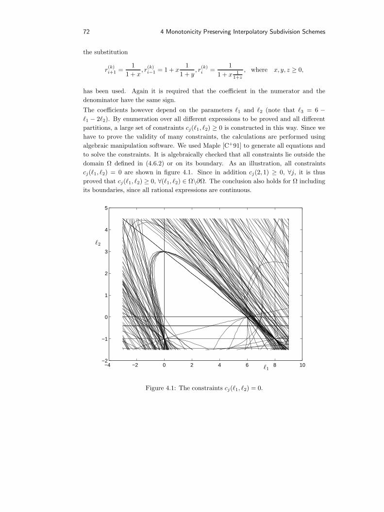
72 4 Monotonicity Preserving Interpolatory Subdivision Schemes
the substitution
r(k)i+1 =
11 + x
, r(k)i−1 = 1 + x
11 + y
, r(k)i =
11 + x 1
1+z
, where x, y, z ≥ 0,
has been used. Again it is required that the coefficient in the numerator and thedenominator have the same sign.
The coefficients however depend on the parameters `1 and `2 (note that `3 = 6 −`1 − 2`2). By enumeration over all different expressions to be proved and all differentpartitions, a large set of constraints cj(`1, `2) ≥ 0 is constructed in this way. Since wehave to prove the validity of many constraints, the calculations are performed usingalgebraic manipulation software. We used Maple [C+91] to generate all equations andto solve the constraints. It is algebraically checked that all constraints lie outside thedomain Ω defined in (4.6.2) or on its boundary. As an illustration, all constraintscj(`1, `2) = 0 are shown in figure 4.1. Since in addition cj(2, 1) ≥ 0, ∀j, it is thusproved that cj(`1, `2) ≥ 0, ∀(`1, `2) ∈ Ω\∂Ω. The conclusion also holds for Ω includingits boundaries, since all rational expressions are continuous.
−4 −2 0 2 4 6 8 10−2
−1
0
1
2
3
4
5
`1
`2
Figure 4.1: The constraints cj(`1, `2) = 0.
4.7 Ratios of first order differences 73
It is thus shown in this proof that
r(k+1)2i+1 ≤ max
r
(k)i , r
(k)i+1
, ∀i and
r(k+1)2i ≤ max
r
(k)i−1, r
(k)i , r
(k)i+1
, ∀i,
which completes the proof.
This result is also maximal in a single step relation between two subsequent subdivisioniterations:
Theorem 4.7.2 Let the numbers r(k) be defined as in theorem 4.7.1. Then, in general,there does not exist a ρ < 1 such that
r(k+1) − 1 ≤ ρ(r(k) − 1).
Proof. Consider the data x(0)i with differences h(0)
i satisfying
h(0)−1 = a, h
(0)0 = b, h
(0)1 = a and h
(0)2 = b, where a > b > 0.
The maximum ratio r(0) is equal to
r(0) =h
(0)1
h(0)0
=a
b> 1,
and because of the symmetry of the scheme, as G(r, r) = 0 (see (4.2.6)), one subdivisionyields
h(1)1 =
b
2, h
(1)2 =
a
2=⇒ r(1) =
h(1)2
h(1)1
=a
b= r(0).
This counterexample shows that the maximum ratio in general does not become smallerin a single subdivision iteration.
Theorem 4.7.2 indicates that we cannot establish convergence of the difference ratiosto 1 using a single step strategy. Next we prove, using a double step strategy, that theratios r(k)
i converge to 1.
Theorem 4.7.3 Let the numbers r(k) be defined as in theorem 4.7.1. Then
r(k+2) − 1 ≤ 34
(r(k) − 1
). (4.7.5)

74 4 Monotonicity Preserving Interpolatory Subdivision Schemes
Proof. It is proved that the r(k+2)j satisfy:
r(k+2)4i−1 − 1 ≤ 5
16
(maxr(k)
i−1, r(k)i , r
(k)i+1 − 1
),
r(k+2)4i − 1 ≤ 3
4
(maxr(k)
i−1, r(k)i , r
(k)i+1 − 1
),
r(k+2)4i+1 − 1 ≤ 5
16
(maxr(k)
i−1, r(k)i , r
(k)i+1 − 1
),
r(k+2)4i+2 − 1 ≤ 1
4
(maxr(k)
i−1, r(k)i , r
(k)i+1, r
(k)i+2 − 1
).
To illustrate the proof, we examine the first pair of inequalities:
516−
r(k+2)4i−1 − 1
maxr(k)i−1, r
(k)i , r
(k)i+1 − 1
≥ 0 and516
+r
(k+2)4i−1 − 1
maxr(k)i−1, r
(k)i , r
(k)i+1 − 1
≥ 0.
Using the same approach as in the proof of theorem 4.7.1, constraints on `1 and `2have been generated. Again, it is algebraically checked that all constraints lie outsidethe domain Ω, see (4.6.2), or on its boundary. This proves that the theorem holds forall (`1, `2) ∈ Ω.The result can be written as
maxj
r
(k+2)j ,
1
r(k+2)j
− 1 ≤ 3
4
(maxj
r
(k)j ,
1
r(k)j
− 1
),
which completes the proof.
Remark 4.7.4 The factors 5/16, 3/4 and 1/4 have at first been conjectured by anasymptotic analysis on arbitrarily chosen data x(0)
i with r(0)i = 1+δiε, where 0 < ε 1
and δi ∈ [−1, 1]. The proofs however, are given for general data.Furthermore, numerical experiments show that the factor 3/4 cannot be improved byoptimising the parameters `1 and `2: all parameter choices within the triangle Ω givethe same contraction factor. ♦
4.8 Convergence of rational subdivision schemes
It is proved in this section that subdivision scheme (4.2.5) with (4.6.1) preserves mono-tonicity and generates continuously differentiable limit functions.
Theorem 4.8.1 (Monotonicity preservation) Subdivision scheme (4.2.5) with G givenin (4.6.1) preserves monotonicity.

4.8 Convergence of rational subdivision schemes 75
Proof. The function G satisfies (4.3.1), which is a direct result from the constructionin section 4.6.
With respect to convergence, the following theorem holds:
Theorem 4.8.2 (C0-convergence) Let the same conditions hold as in theorem 4.4.1.Then, repeated application of subdivision scheme (4.2.5) with (4.6.1) leads to a contin-uous function which is monotone and interpolates the initial data points (t(0)
i , x(0)i ), if
`2 > 0 or the initial data are strictly monotone.
Proof. First, if `2 > 0, it is shown that G satisfies
|G(r,R)| =∣∣∣∣ r −R`1 + (1 + `2)(r +R) + `3rR
∣∣∣∣ ≤ r +R
`1 + (1 + `2)(r +R) + `3rR
≤ r +R
(1 + `2)(r +R)=
11 + `2
= µ < 1, (4.8.1)
i.e., G satisfies condition (4.4.1).If the initial data are strictly monotone, we remark that the ratios of first order differ-ences r(k)
i can be estimated using theorem 4.7.1:
1 ≤ maxi
max
r
(k)i ,
1
r(k)i
≤ r(0) <∞.
The function G defined in (4.6.1) is monotone in both arguments, see remark 4.6.3, andhence is maximal in the case r(k)
i = r(0) and R(k)i+1 = 1/r(0), which yields that G can be
estimated as
|G(r(k)i , R
(k)i+1)| ≤ (r(0))2 − 1
(`1 + `3)r(0) + (1 + `2)((r(0))2 + 1)= µ < 1, (4.8.2)
which proves (4.4.1) for all (`1, `2, `3) ∈ Ω, as r(0) <∞.
Concerning C1-convergence, we can formulate the following result:
Theorem 4.8.3 (C1-convergence) Let the same conditions hold as in theorem 4.5.1,and let the data be strictly monotone.Then repeated application of subdivision scheme (4.2.5) with (4.6.1) leads to a continu-ously differentiable function which is monotone and interpolates the initial data points(t(0)i , x
(0)i ).
Proof. As the function G is continuously differentiable in r and R, for all r,R ≥ 0,it satisfies Lipschitz-condition (4.5.1). It is shown in section 4.7 that this function

76 4 Monotonicity Preserving Interpolatory Subdivision Schemes
G yields that ratios of adjacent first order differences converge to 1, i.e., the C1-requirement (4.5.2) is satisfied.
The analysis of the subdivision scheme for monotone, but not strictly monotone datais more difficult to examine. At any dyadic point the left and right derivative canbe proved to be equal, but this is not sufficient for convergence to a continuouslydifferentiable limit function. Numerical experiments however show that the subdivisionscheme yields limit functions that are continuously differentiable even in such cases:
Conjecture 4.8.4 (Always C1) Let the same conditions hold as in theorem 4.5.1, butlet the data be monotone but not necessarily strictly monotone.Repeated application of subdivision scheme (4.2.5) with (4.6.1) leads to a continu-ously differentiable function which is monotone and interpolates the initial data points(t(0)i , x
(0)i ).
In the following example we show the graphical capabilities of the subdivision schemeand illustrate tension control that is provided by the parameters `1, `2 and `3.
Example 4.8.5 (Numerical example) Consider the equidistant data set defined in ta-ble 4.1. Some visual results are shown after repeated application of subdivision scheme(4.2.5) with G in (4.6.1).
t(0)i -2 -1 0 1 2 3 4 5 6 7 8
x(0)i -2 -1 0 1/2 1 6 6 7 8 9 10
Table 4.1: The data set used in the numerical example.
First, the limit function is shown in the interval [t(0)0 , t
(0)6 ] for the monotonicity pre-
serving scheme with the parameter choice `1 = 2, `2 = 1 and `3 = 2, see remark 4.6.4,which has proved to generate results that are visually pleasing. This result is comparedwith the graphical performance of the linear four-point scheme [DGL87], see (4.3.4), infigure 4.2, which clearly does not preserve monotonicity for this data set.In the next plots, see figure 4.3, we again display the limit function of the monotonicitypreserving subdivision scheme with `1 = 2, `2 = 1 and `3 = 2, together with itsderivative, which is nonnegative in the whole interval.Finally, it is shown in figure 4.4 that the parameters `j act as tension parameters. Twoextreme choices are compared: `1 = 0, `2 = 0, `3 = 6 and `1 = 3, `2 = 3/2, `3 = 0respectively. The first case leads to a limit function that is almost piecewise constant indifficult areas, whereas the second choice of the tension parameters leads to an almost

4.9 Stability and Approximation order 77
0 1 2 3 4 5 60
1
2
3
4
5
6
7
8
x(∞)
t0 1 2 3 4 5 6
0
1
2
3
4
5
6
7
8
x(∞)
t
Figure 4.2: The limit function obtained by the monotonicity preserving scheme (with`1 = 2, `2 = 1, `3 = 2) and the linear four-point scheme.
0 1 2 3 4 5 60
1
2
3
4
5
6
7
8
x(∞)
t0 1 2 3 4 5 6
−1
0
1
2
3
4
5
6
7
y(∞)
t
Figure 4.3: The limit function x(∞) and its derivative y(∞) obtained by the monotonic-ity preserving scheme (with `1 = 2, `2 = 1, `3 = 2).
piecewise linear function. ♦
4.9 Stability and Approximation order
In this section, the stability and the approximation properties of the monotonicity pre-serving subdivision schemes from the previous sections are examined. Although a sim-ple calculation shows that the scheme only reproduces linear functions (and quadratics

78 4 Monotonicity Preserving Interpolatory Subdivision Schemes
0 1 2 3 4 5 60
1
2
3
4
5
6
7
8
x(∞)
t0 1 2 3 4 5 6
0
1
2
3
4
5
6
7
8
x(∞)
t
Figure 4.4: Tension control illustrated by the limit function obtained by the mono-tonicity preserving scheme with `1 = 0, `2 = 0, `3 = 6 and `1 = 3, `2 = 3/2, `3 = 0respectively.
in the case `3 = 0), it can be proved that the scheme has approximation order four.
Theorem 4.9.1 (Stability) Let G : IR2 → IR be C1 and homogeneous of degree 0 in itsarguments. Then interpolatory subdivision schemes in the class (4.2.5) which preservestrict monotonicity and which satisfy (4.5.2), are stable.
Proof. The proof follows the same lines as the proof of theorem 3.5.1. For the sake ofsimplicity, we write
F(h(k)i−1, h
(k)i , h
(k)i+1) =
12h
(k)i G(r(k)
i , R(k)i+1).
The essential ingredients are that the sum over the three partial derivatives of F canbe bounded by ±ρ/2 for sufficiently large k. Secondly, Euler’s identity gives∣∣∣F(h(k)
i−1, h(k)i , h
(k)i+1)−F(h(k)
i−1, h(k)i , h
(k)i+1)
∣∣∣ ≤ |F1 + F2 + F3|maxi
∣∣∣h(k)i − h
(k)i
∣∣∣ ,where Fj denotes the partial derivative of F with respect to its j-th argument.Finally, one can prove that∣∣∣h(k+1)
2i+j − h(k+1)2i+j
∣∣∣ ≤ 12
∣∣∣h(k)i − h
(k)i
∣∣∣± ∣∣∣F(h(k)i−1, h
(k)i , h
(k)i+1) + F(h(k)
i−1, h(k)i , h
(k)i+1)
∣∣∣≤(
12
+ρ
2
)maxi
∣∣∣h(k)i − h
(k)i
∣∣∣ ,which shows stability, as ρ < 1.

4.10 Generalisations 79
Remark 4.9.2 Theorem 4.9.1 is also easily shown to be valid for monotone schemeswhich are less local, e.g., six-point schemes, provided the ratios r(k)
i converge suffi-ciently fast to 1. ♦
Using the results from section 4.6 and application of theorem 2.4.10, one gets:
Corollary 4.9.3 Subdivision scheme (4.2.5) with (4.6.1) has approximation order four.
An alternative proof can be found in [KvD97a].
Remark 4.9.4 Observe that this analysis is only valid for strictly monotone data, i.e.,data drawn from a function g with g′(τ) > 0, ∀τ ∈ I. Numerical experiments showthat if g′(τ) = 0 for some τ ∈ I, the approximation order in the max-norm decreasesto 3. ♦
4.10 Generalisations
In this section, we briefly describe an extension and look forward to generalisations ofthe monotonicity preserving subdivision scheme discussed in this chapter.
Piecewise monotonicity. The subdivision scheme discussed in this chapter can beextended to a piecewise monotonicity preserving subdivision scheme suited for inter-polation of piecewise monotone data.We first observe that any monotonicity preserving subdivision scheme of the form (4.2.5)is also directly applicable to monotone decreasing data. It is therefore only necessaryto examine regions in the initial data where the differences h(0)
i change sign and to splitthe domain in monotone increasing parts and monotone decreasing parts.If one of the differences in the initial data is zero, i.e., the case that the differences satisfyh
(0)0 = 0, h(0)
−1 < 0 and h(0)1 > 0, a simple and natural way to split the monotonicity
regions is provided by the data: the solution in the interval [t(0)0 , t
(0)1 ] becomes constant.
The monotonicity preserving subdivision scheme can be applied both on the left-hand-side of t(0)
0 and on the right-hand-side of t(0)1 . The limit function is then monotone
decreasing left to t(0)1 and monotone increasing right to t
(0)0 . In fact, the scheme is
piecewise monotonicity preserving for these data.The general case is characterised by data with differences satisfying h(0)
−2 < 0, h(0)−1 < 0,
h(0)0 > 0 and h
(0)1 > 0, since all other cases degenerate to this situation after one
iteration. We define the split point as the point where the differences change sign, i.e.,in this case t(0)
0 .

80 4 Monotonicity Preserving Interpolatory Subdivision Schemes
A simple method to adapt the subdivision scheme to piecewise monotonicity preserva-tion is as follows:
• Apply the monotonicity preserving subdivision scheme to determine x(k)j for j <
0, where h(0)0 is replaced by 0.
• Apply the monotonicity preserving subdivision scheme to determine x(k)j for j >
0, where h(0)−1 is replaced by 0.
The corresponding function GPM of this piecewise monotonicity preserving subdivisionscheme can be written as
GPM (r,R) = G (max0, r,max0, R) ,
with e.g., G defined as in (4.6.1).It is clear that the limit function is monotone decreasing for t ≤ t
(0)0 and monotone
increasing for t ≥ t(0)0 . The derivative of the limit function in t
(0)0 is equal to zero.
Convergence to a continuously differentiable limit function is achieved if conjecture 4.8.4is true.
Connection with monotone splines. An alternative way to derive subdivision scheme(4.2.5) with G as in (4.6.5) originates from Hermite interpolation using quadraticsplines, see [Sch83, Iqb92].Consider a strictly monotone data set (2−ki, x(k)
i )i and define Bezier points as follows
b(k)2i = x
(k)i , b
(k)2i+1 = x
(k)i +
2−k
4ξ
(k)i , b
(k)2i+3 = x
(k)i+1 −
2−k
4ξ
(k)i+1, and b
(k)2i+4 = x
(k)i+1,
where the ξ(k)i are suitable derivative estimates.
Define now the subdivision points x(k+1)2i+1 as follows
x(k+1)2i+1 = b
(k)2i+2 =
12
(b2i+1 + b2i+3) =12
(x
(k)i + x
(k)i+1
)+
2−k
8
(ξ
(k)i − ξ
(k)i+1
). (4.10.1)
If the derivatives are estimated as in [But80,FB84], i.e.,
ξ(k)j = 2
∆x(k)j−1∆x(k)
j
∆x(k)j−1 + ∆x(k)
j
, with ∆x(k)i = 2kh(k)
i ,
then subdivision scheme (4.10.1) preserves monotonicity and is written as
x(k+1)2i+1 =
12
(x
(k)i + x
(k)i+1
)+
14h
(k)i
(h
(k)i−1
h(k)i−1 + h
(k)i
−h
(k)i+1
h(k)i + h
(k)i+1
)
=12
(x
(k)i + x
(k)i+1
)+
12h
(k)i GB(r(k)
i , R(k)i+1),
4.10 Generalisations 81
with
GB(r(k)i , R
(k)i+1) =
12
(h
(k)i−1
h(k)i−1 + h
(k)i
−h
(k)i+1
h(k)i + h
(k)i+1
)
=12
(h
(k)i
h(k)i + h
(k)i+1
− h(k)i
h(k)i−1 + h
(k)i
)=
12
(1
1 +R(k)i+1
− 1
1 + r(k)i
),
which coincides with the special case GC in (4.6.5), see remark 4.6.4.In fact this approach does not only define a subdivision scheme, but the constructionusing Bezier points also provides an explicit interpolation method using monotonicitypreserving quadratic (B-)splines.
Remark 4.10.1 Note that the Butland-slope is the harmonic average of two adjacentfirst differences, whereas the convexity preserving subdivision scheme from chapter 3is a scheme that contains the harmonic average of two second order differences. ♦
A relation between rational interpolation and convexity preserving subdivision is ob-served in [FM98]. There exists also a connection between monotonicity preservingrational interpolation and subdivision scheme (4.2.5) with (4.6.1). In [GD82], a classof rational splines is defined on an interval [ti, ti+1] as follows
xi(t) =∆xixi+1θ
2 + (xiξi+1 + xi+1ξi) θ(1− θ) + ∆xixi(1− θ)2
∆xiθ2 + (ξi+1 + ξi)θ(1− θ) + ∆xi(1− θ)2 ,
whereθ =
t− titi+1 − ti
and ∆xi =xi+1 − xiti+1 − ti
,
and the ξj are suitable chosen derivative estimates at tj .The construction is restricted to equidistant data, and a subdivision scheme is obtainedby halfway evaluation of xi(t), i.e., at t(k+1)
2i+1 = 12 (t(k)
i + t(k)i+1). This results in the
subdivision scheme
x(k+1)2i+1 = x(t(k+1)
2i+1 ) =12
(x
(k)i + x
(k)i+1
)+
12h
(k)i
ξ(k)i+1 − ξ
(k)i
ξ(k)i + 2∆x(k)
i + ξ(k)i+1
,
Two choices for the derivative estimates ξ(k)j are presented: the arithmetic mean and
the harmonic mean.
ξ(k)j =
12
(∆x(k)
j−1 + ∆x(k)j
), or ξ
(k)j =
2∆x(k)j−1∆x(k)
j
∆x(k)j−1 + ∆x(k)
j
,

82 4 Monotonicity Preserving Interpolatory Subdivision Schemes
and both choices yield a subdivision scheme as in (4.2.5), and the functions GL and GBare respectively given by
GL(r,R) =r −R
6 + r +R, and GB(r,R) =
r −R1 + 2(r +R) + 3rR
,
Both functions are contained in the class (4.6.1), as (`1, `2, `3) = (6, 0, 0) ∈ Ω, and(`1, `2, `3) = (1, 1, 3) ∈ Ω.

Chapter 5
Shape Preserving InterpolatorySubdivision Schemes for NonuniformData
5.1 Introduction
This chapter deals with a class of shape preserving four-point subdivision schemeswhich are stationary and which interpolate nonuniform univariate data (xi, fi) ∈IR2, where the x-data are strictly monotone, i.e., xj < xj+1, ∀j. The basic ideain the construction is to distinguish between subdivision of the x-data and the f -data. First, a suitable scheme for the x-values is defined. Then a subdivision schemefor the f -values is constructed, which depends on the choice of x-subdivision. Thisleads to nonuniform interpolatory subdivision schemes, i.e., schemes for interpolationof nonuniform, or nonequidistant, data. We require that these schemes are stationaryand that they use (at most) four points, i.e., the schemes are local.The contents of this chapter is as follows. First, in section 5.2 the problem definition isgiven, some basic definitions are introduced, and the subdivision scheme for the x-datais discussed. As the data are univariate and nonequidistant, the x-values have to besubdivided in a monotonicity preserving way. This is discussed in section 5.2.2. Theclass of monotonicity preserving interpolatory subdivision schemes examined in chapter4 is attractive for this purpose, since it is capable of generating grids x(k)
i that, in thelimit, become locally uniform. Although it is only necessary for (C0-)convergence thatthe grid becomes dense, see e.g., [GQ96] and [DGS97], this stronger property turns outto be helpful for the C1-convergence analysis of the limit function.Having treated the subdivision scheme for the x-data, a class of nonuniform subdivisionschemes that possesses some natural requirements, see e.g., [CD94], is characterised.
84 5 Shape Preserving Interpolatory Subdivision Schemes for Nonuniform Data
This class of schemes is further restricted to a class of nonuniform subdivision schemesthat preserve convexity, but actually any shape e.g., monotonicity can be treated in asimilar way. A sufficient condition for preservation of convexity is given in section 5.3.All subdivision schemes that satisfy this condition automatically generate continuouslimit functions. In addition, in section 5.4, sufficient conditions for convergence to aconvex and continuously differentiable limit function are given, provided the data arestrictly convex. These conditions lead to an explicit class of subdivision schemes thatare rational in their arguments, and that generate continuously differentiable functions.The class of schemes is further restricted to schemes that reproduce quadratic polyno-mials, with which it is proved that they are third order accurate, see section 5.5. Forequidistant data, all schemes in this class reduce to the convexity preserving subdivisionscheme introduced in chapter 3. A connection with rational interpolation is discussed.
In section 5.6 a convexity preserving midpoint subdivision scheme is proved to gen-erate continuously differentiable limit functions, but this scheme is only second orderaccurate.
Apart from convexity preserving nonuniform subdivision schemes, we examine linearschemes for nonequidistant data in section 5.7. These schemes are linear in the f -databut are still nonlinear in the parameter values x(k)
i . A nonuniform extension of thewell-known linear four-point scheme [DGL87] is constructed. This generalised linearscheme does not loose accuracy in case of nonuniform data, i.e., the approximationorder is still equal to four. The important difference with other papers, e.g., [DGS97],is that subdivision for the x-values is performed by a simple stationary, rational subdi-vision scheme. The fact that the scheme for subdivision of the x-values is nonlinear isnot problematic as the scheme for the f -values is still linear. Smoothness of the limitfunction generated by these linear schemes is proved by using the well-known smooth-ness criteria of the uniform linear four-point scheme. In addition, the approximationorder of nonuniform linear schemes is examined.
Finally, some numerical examples illustrate nonuniform convexity preserving subdivi-sion.
5.2 Nonuniform subdivision
In this section, the problem definition is given and some basic definitions are introduced,see section 5.2.1. The method for x-subdivision is discussed in section 5.2.2, and aclass of nonuniform subdivision schemes with natural requirements is constructed insection 5.2.3.

5.2 Nonuniform subdivision 85
5.2.1 Problem definition
The problem examined in this chapter is stated. Given is a univariate initial dataset (x(0)
i , f(0)i ) ∈ IR2, where the x(0)
i are strictly monotone, i.e., x(0)i < x
(0)i+1, ∀i.
The uniformly distributed dyadic points t(k)i are defined by t
(k)i = 2−ki. The dataset
(t(k)i , x
(k)i )i is then uniform and strictly monotone.
A class of nonuniform interpolatory subdivision schemes for the data (x(0)i , f
(0)i ) must
be characterised. The aim is to construct nonuniform convexity preserving subdivisionschemes. This class of schemes has to be restricted to subdivision schemes that generateconvex and continuously differentiable limiting functions. The second goal is to obtainmaximal order of approximation for these schemes.The approach in this chapter is to subdivide the x-values by a monotonicity preservinginterpolatory subdivision scheme. The class of schemes examined in chapter 4 is usedfor this purpose. This choice is discussed in section 5.2.2, but first we introduce somebasic definitions.
5.2.2 Monotonicity preservation
In this section, the results from chapter 4 are applied for the purpose of nonuniformunivariate interpolatory subdivision schemes.The initial data x(0)
i are strictly monotone, and a simple linear scheme that pre-serves monotonicity is given by the two-point scheme (2.3.2). This scheme is calledthe midpoint scheme, and it satisfies the property that the grid becomes dense, seee.g., [GQ96] and [DGS97]. In [GQ96], the authors discuss nonuniform corner cuttingand the necessity that the grid becomes dense, but their results cannot directly be usedfor interpolatory subdivision.In chapter 4, we examined four-point interpolatory subdivision schemes for equidistantdata that preserve monotonicity. The class of schemes that was examined is charac-terised by (4.2.5), and G is a function that satisfies specific properties discussed inchapter 4. The first condition (4.3.1) ensures monotonicity preservation, and a second(stronger) condition on G is that subdivision scheme (4.2.5) has the property that itgenerates grids x(k)
i that become locally uniform in the following sense:
r(k) := maxi
maxr
(k)i , 1/r(k)
i
≤ 1 +A0ρ
k0 , ∀k, ρ0 < 1, A0 <∞. (5.2.1)
This property of generating locally uniform grids is attractive as it turns out to besuited for the C1-convergence analysis of nonuniform subdivision schemes. The initialdata are assumed to be strictly monotone, and condition (5.2.1) then yields that 1 ≤r(k) ≤ r(0) <∞.The class of functions G in theorem 4.6.1 provides explicit rational monotonicity pre-serving subdivision schemes that satisfy the demanded properties (4.3.1) and (5.2.1).

86 5 Shape Preserving Interpolatory Subdivision Schemes for Nonuniform Data
This class of monotonicity preserving subdivision schemes has approximation order fourwhen applied to equidistant data (t(0)
i , x(0)i ), see chapter 4. For this chapter, a more
important property, see chapter 4, is that the scheme with (4.6.1) satisfies (5.2.1), asthe scheme satisfies (4.7.2) and (4.7.5), i.e., A0 =
√4/3 and ρ0 =
√3/4 in (5.2.1), and
the grid becomes locally uniform.
5.2.3 Nonuniform subdivision schemes
In this section we construct a class of subdivision schemes for interpolation of nonuni-form functional data (x(k)
i , f(k)i ). The x-values are subdivided using (4.2.5) for gen-
eral G satisfying (4.3.1).The general class of nonuniform subdivision schemes is written as:
x(k+1)2i = x
(k)i ,
x(k+1)2i+1 =
12
(x
(k)i + x
(k)i+1
)+
12h
(k)i G(r(k)
i , R(k)i+1),
f(k+1)2i = f
(k)i ,
f(k+1)2i+1 = F1(f (k)
i−1, f(k)i , f
(k)i+1, f
(k)i+2, x
(k)i−1, x
(k)i , x
(k)i+1, x
(k)i+2).
(5.2.2)
This implies:
1. The subdivision schemes are interpolatory.
2. The subdivision schemes are local, using four points.
Define f (k+1)2i+1 as the linear interpolant to the data points (x(k)
i , f(k)i ) and (x(k)
i+1, f(k)i+1),
which is evaluated at the parameter x(k+1)2i+1 determined by scheme (4.2.5):
f(k+1)2i+1 =
(x(k)i+1 − x
(k+1)2i+1 )f (k)
i + (x(k+1)2i+1 − x
(k)i )f (k)
i+1
x(k)i+1 − x
(k)i
=h
(k+1)2i+1 f
(k)i + h
(k+1)2i f
(k)i+1
h(k)i
=12
(f
(k)i + f
(k)i+1
)+
12G(r(k)
i , R(k)i+1)
(f
(k)i+1 − f
(k)i
). (5.2.3)
Then, f (k+1)2i+1 can also be written as
f(k+1)2i+1 = f
(k+1)2i+1 −F2(f (k)
i−1, f(k)i , f
(k)i+1, f
(k)i+2, x
(k)i−1, x
(k)i , x
(k)i+1, x
(k)i+2).
Additional conditions on the correction function F2 are determined by the followingassumptions on the subdivision schemes:
5.2 Nonuniform subdivision 87
3. The subdivision schemes are invariant under addition of linear functions, i.e.,if the data (x(0)
i , f(0)i ) generate subdivision points (x(k)
i , f(k)i ), then the data
(x(0)i , f
(0)i +λx
(0)i +µ), with λ, µ ∈ IR yield subdivision points (x(k)
i , f(k)i +λx
(k)i +
µ).
4. The subdivision schemes are invariant under affine transformations of the vari-ables x(0)
i , i.e., if the initial data (x(0)i , f
(0)i ) yield subdivision points (x(k)
i , f(k)i ),
then the data (λx(0)i + µ, f
(0)i ), with λ, µ ∈ IR, λ 6= 0, yield subdivision points
(λx(k)i + µ, f
(k)i ).
Condition 4 with λ = 1, combined with condition 3, yields that the scheme can bewritten as
f(k+1)2i+1 = f
(k+1)2i+1 − F3(s(k)
i , s(k)i+1, h
(k)i−1, h
(k)i , h
(k)i+1).
The following assumption deals with homogeneity:
5. The subdivision schemes are homogeneous, i.e., if initial data (x(0)i , f
(0)i ) gen-
erate subdivision points (x(k)i , f
(k)i ), then initial data (x(0)
i , λf(0)i ) yield points
(x(k)i , λf
(k)i ).
A direct consequence of homogeneity of the subdivision scheme is then that the functionF3 is homogeneous:
F3(λx, λy, a, b, c) = λF3(x, y, a, b, c), ∀λ. (5.2.4)
The homogeneity of F3 combined with assumption 4 with µ = 0 yields
F3(1λx,
1λy, λa, λb, λc) = F3(x, y, a, b, c), ∀λ,
and this gives homogeneity in the last three arguments of F3:
F3(x, y, λa, λb, λc) = λF3(x, y, a, b, c), ∀λ.
Using the homogeneity, the function F is defined by
F3(s(k)i , s
(k)i+1, h
(k)i−1, h
(k)i , h
(k)i+1) = h
(k)i F(s(k)
i , s(k)i+1, r
(k)i , R
(k)i+1).
The final assumption is:
6. The function F is Lipα, α > 0, in all its arguments.

88 5 Shape Preserving Interpolatory Subdivision Schemes for Nonuniform Data
The class of nonuniform interpolatory subdivision schemes examined in this chapterbecomes:
x(k+1)2i = x
(k)i ,
x(k+1)2i+1 =
12
(x
(k)i + x
(k)i+1
)+
12h
(k)i G(r(k)
i , R(k)i+1),
f(k+1)2i = f
(k)i ,
f(k+1)2i+1 = f
(k+1)2i+1 − h
(k)i F(s(k)
i , s(k)i+1, r
(k)i , R
(k)i+1),
(5.2.5)
where f (k+1)2i+1 is the piecewise linear interpolant defined in (5.2.3).
Remark 5.2.1 (Symmetry) The invariance under affine transformations of the vari-ables necessarily yields (take λ = −1 and µ = 0 in assumption 4) that F obeys thefollowing symmetry:
F(x, y, r, R) = F(y, x,R, r). (5.2.6)
Remark 5.2.2 (Reproduction of linear functions) Homogeneity of F , see (5.2.4), yieldsthat
F(λx, λy, r, R) = λF(x, y, r, R),
and taking λ = 0 yields F(0, 0, r, R) = 0, i.e., subdivision scheme (5.2.5) automaticallyreproduces linear functions. ♦
5.2.4 Example: A nonuniform linear four-point scheme
As an example of nonuniform subdivision on a grid that becomes locally uniform, anonuniform linear scheme is constructed in this section.
Definition 5.2.3 (Linearity) We call a subdivision scheme of the class (5.2.5) linear,if the function F(x, y, r, R) is linear in the variables x and y, i.e., we can write F as
F(x, y, r, R) = K1(r,R)x+K2(r,R)y. (5.2.7)
A linear subdivision scheme for non-equidistant data will be constructed as a generalisa-tion of the uniform linear four-point scheme [DGL87] with w = 1/16. This scheme canbe interpreted as the interpolating cubic polynomial through four successive equidis-tant data points. We therefore determine the cubic polynomial that interpolates thefour non-equidistant data points (x(k)
i−1, f(k)i−1), (x(k)
i , f(k)i ), (x(k)
i+1, f(k)i+1) and (x(k)
i+2, f(k)i+2).
The value of f (k+1)2i+1 is defined as the evaluation of this cubic interpolating function at
x(k+1)2i+1 .

5.3 Convexity preservation 89
A straightforward calculation yields that the resulting linear subdivision scheme fornon-equidistant data is contained in the class (5.2.5) with FL given by (5.2.7), wherethe functions K1
L and K2L satisfy (subscripts L refer to linear)K1L(r,R)=
18
1− G2(r,R)1 + r +R
1− G(r,R) + 2R1 + r
,
K2L(r,R)=
18
1− G2(r,R)1 + r +R
1 + G(r,R) + 2r1 +R
.
(5.2.8)
where G is assumed to be chosen such that condition (5.2.1) is satisfied.Analogous to the linear four-point scheme [DGL87] for general w, a class of nonuniformlinear interpolatory four-point schemes is now:
f(k+1)2i = f
(k)i ,
f(k+1)2i+1 = f
(k)2i+1 − 16wh(k)
i
(K1L(r(k)
i , R(k)i+1)s(k)
i +K2L(r(k)
i , R(k)i+1)s(k)
i+1
).
(5.2.9)
When the tension parameter equals w = 1/16, the scheme reproduces cubic polynomi-als, and the functions K1
L and K2L are then given in (5.2.8).
In the limit k → ∞, the nonuniform linear scheme converges to the uniform linearscheme, as the ratios defined in (2.1.4) satisfy r
(k)i → 1, and the functions in (5.2.9)
satisfy G → 0, KjL → 1/16, i.e., the scheme for equidistant data becomes:
f(k+1)2i+1 =
12
(f
(k)i + f
(k)i+1
)− wh(k)
i (s(k)i + s
(k)i+1)
= − wf (k)i−1 +
(12
+ w
)f
(k)i +
(12
+ w
)f
(k)i+1 − wf
(k)i+2, (5.2.10)
and this is the linear four-point scheme in [DGL87]. It is proved in [DGL87], usinga double step estimate on jumps of divided differences s(k)
j , that it is sufficient forconvergence to C1 limit functions that 0 < w < 1/8, and this range on the tensionparameter can also be enlarged using more steps, see e.g., [DGL91].In section 5.7, properties of nonuniform linear subdivision schemes in the class (5.2.7)are discussed. In the next sections, we discuss convexity preserving subdivision schemesand analyse the smoothness properties of the limit function and its approximationorder.
5.3 Convexity preservation
In this section, we examine convexity preservation of the class of nonuniform subdivisionschemes (5.2.5). A sufficient condition for preservation of convexity is given in thefollowing theorem:

90 5 Shape Preserving Interpolatory Subdivision Schemes for Nonuniform Data
Theorem 5.3.1 (Sufficient convexity condition) Let β ∈ Lipα(IR+), α > 0, be afunction such that it holds for all r ∈ IR+ that
β(r) ≥ 0 and β(r) + β(1/r) ≤ 2. (5.3.1)
Then, subdivision scheme (5.2.5) satisfying (4.3.1) and
0 ≤ F(x, y, r, R) ≤ 14
min β(r) (1 + G(r,R)) x, β(R) (1− G(r,R)) y , (5.3.2)
preserves convexity.
Proof. Consider the data (x(k)i , f
(k)i ) ∈ IR2 generated by subdivision scheme (5.2.5)
where G satisfies (4.3.1). Convexity preserving properties of (5.2.5) are analysed byexamining second order differences s(k)
i : the jumps in the first order divided differencesmust be nonnegative. The first order divided differences satisfy
∆f (k+1)2i = ∆f (k)
i − 2F(s(k)
i , s(k)i+1, r
(k)i , R
(k)i+1)
1 + G(r(k)i , R
(k)i+1)
and similarly (5.3.3)
∆f (k+1)2i+1 = ∆f (k)
i + 2F(s(k)
i , s(k)i+1, r
(k)i , R
(k)i+1)
1− G(r(k)i , R
(k)i+1)
, (5.3.4)
and the second order differences s(k+1)2i+1 and s
(k+1)2i become:
s(k+1)2i+1 = ∆f (k+1)
2i+1 −∆f (k+1)2i = 4
F(s(k)i , s
(k)i+1, r
(k)i , R
(k)i+1)
1− G2(r(k)i , R
(k)i+1)
, (5.3.5)
s(k+1)2i = s
(k)i − 2
F(s(k)i , s
(k)i+1, r
(k)i , R
(k)i+1)
1 + G(r(k)i , R
(k)i+1)
− 2F(s(k)
i−1, s(k)i , r
(k)i−1, R
(k)i )
1− G(r(k)i−1, R
(k)i )
. (5.3.6)
It has to be proved for convexity that s(k+1)i ≥ 0, if s(k)
i ≥ 0.Since G satisfies (4.3.1), non-negativity of s(k+1)
2i+1 is equivalent to non-negativity of F :
F(x, y, r, R) ≥ 0, ∀x, y ≥ 0, ∀r,R > 0.
As (4.3.1) holds and β is nonnegative, this lower bound on F is necessary and sufficientfor s(k+1)
2i+1 ≥ 0.The second part, the non-negativity of s(k+1)
2i , is obtained as follows:
s(k+1)2i = s
(k)i −
2F(s(k)i , s
(k)i+1, r
(k)i , R
(k)i+1)
1 + G(r(k)i , R
(k)i+1)
−2F(s(k)
i−1, s(k)i , r
(k)i−1, R
(k)i )
1− G(r(k)i−1, R
(k)i )
≥ s(k)i −
2
1 + G(r(k)i , R
(k)i+1)
14
(1 + G(r(k)
i , R(k)i+1)
)β(r(k)
i )s(k)i

5.4 Convergence to a continuously differentiable function 91
− 2
1− G(r(k)i−1, R
(k)i )
14
(1− G(r(k)
i−1, R(k)i ))β(R(k)
i )s(k)i
= s(k)i
(1− 1
2β(r(k)
i )− 12β(R(k)
i ))≥ 0,
which completes the proof.
Example 5.3.2 An example of a function β that satisfies (5.3.1) is
β(r) = 21− α+ αr
1 + r, for 0 ≤ α ≤ 1,
as
β(r) ≥ 0 and β(r) + β(1/r) = 21− α+ αr
1 + r+ 2
(1− α)r + α
1 + r= 2.
The special case β(r) = 1 is obtained by the choice α = 1/2. ♦
Theorem 5.3.3 (Convergence) Given is a convex data set (x(0)i , f
(0)i ) ∈ IR2, where
x(0)i is strictly monotone. The k-th stage data (x(k)
i , f(k)i )i are defined by subdivi-
sion scheme (5.2.5) with (4.3.1) where F satisfies the convexity conditions (5.3.1) and(5.3.2).Repeated application of such a subdivision scheme generates a continuous functionwhich is convex and interpolates the initial data points (x(0)
i , f(0)i ).
Proof. Define the function f (k) as the piecewise linear interpolant to the data (x(k)i , f
(k)i ).
The sequence of functions f (k) is a bounded and monotone decreasing sequence of con-tinuous functions. In addition, condition (4.3.1) yields that the grid x(k)
i becomesdense. Therefore, the limit function f (∞) exists and is continuous.
5.4 Convergence to a continuously differentiable function
In this section, we first present a lemma dealing with a sufficient condition for con-vergence of subdivision schemes of the class (5.2.5) to continuously differentiable limitfunctions. This lemma is applied to subdivision schemes that preserve convexity.
Lemma 5.4.1 (Sufficient smoothness conditions) Given is a data set (x(0)i , f
(0)i ) ∈
IR2, where x(0)i is strictly monotone. The k-th stage data (x(k)
i , f(k)i ) are defined
by subdivision scheme (5.2.5) where G satisfies (4.3.1).

92 5 Shape Preserving Interpolatory Subdivision Schemes for Nonuniform Data
A sufficient condition for convergence of such a subdivision scheme to a continuouslydifferentiable limit function is that the quantities
maxi|s(k)i |
form a Cauchy sequence in k with limit 0.
Proof. The construction follows the lines of the proof of smoothness of the limit functiongenerated by the linear four-point scheme [DGL87], as we did in chapter 3. For anydata set (x(k)
i , f(k)i ), the function g(k) is defined as the linear interpolant of the data
points (x(k+1)2i+1 ,∆f
(k)i ), where ∆f (k)
i are first order divided differences, see (2.1.6).It is sufficient for convergence of this sequence g(k) that there exists a C1 ∈ IR andµ1 < 1 (where µ1 may depend on the initial data), such that
‖g(k+1) − g(k)‖∞ ≤ C1µk1. (5.4.1)
By construction, the maximal distance between the functions g(k) and g(k+1) occurs ata point x(k+2)
4i−1 or x(k+2)4i+1 for some i, i.e., it must hold that
‖g(k+1) − g(k)‖∞ = maxi
maxδ(k+1)2i−1 , δ
(k+1)2i ≤ C1µ
k1 ,
where the distances δ(k)j are given by
δ(k+1)2i−1 =
∣∣∣∣∣∆f (k+1)2i−1 −
(h(k+2)4i−1 + h
(k+1)2i )∆f (k)
i−1 + h(k+2)4i−2 ∆f (k)
i
h(k+1)2i−1 + h
(k+1)2i
∣∣∣∣∣ and
δ(k+1)2i =
∣∣∣∣∣∆f (k+1)2i −
h(k+2)4i+1 ∆f (k)
i−1 + (h(k+1)2i−1 + h
(k+2)4i )∆f (k)
i
h(k+1)2i−1 + h
(k+1)2i
∣∣∣∣∣ .Since ∆f (k+1)
2i satisfies (5.3.3) and similarly
∆f (k+1)2i−1 = ∆f (k)
i−1 + 2F(s(k)
i−1, s(k)i , r
(k)i−1, R
(k)i )
1− G(r(k)i−1, R
(k)i )
,
it is obtained after some straightforward calculations that
δ(k+1)2i =
∣∣∣∣∣12 h(k+1)2i
(1− G(r(k+1)
2i , R(k+1)2i+1 )
)h
(k+1)2i−1 + h
(k+1)2i
s(k)i − 2
F(s(k)i , s
(k)i+1, r
(k)i , R
(k)i+1)
1 + G(r(k)i , R
(k)i+1)
∣∣∣∣∣ ,which can be further bounded by
δ(k+1)2i ≤
∣∣∣∣∣12 h(k+1)2i
(1− G(r(k+1)
2i , R(k+1)2i+1 )
)h
(k+1)2i−1 + h
(k+1)2i
s(k)i
∣∣∣∣∣+
∣∣∣∣∣2F(s(k)i , s
(k)i+1, r
(k)i , R
(k)i+1)
1 + G(r(k)i , R
(k)i+1)
∣∣∣∣∣≤ 1
2· 2 · 1 · |s(k)
i |+2
1− µG
∣∣∣F(s(k)i , s
(k)i+1, r
(k)i , R
(k)i+1)
∣∣∣= |s(k)
i |+2
1− µG
∣∣∣F(s(k)i , s
(k)i+1, r
(k)i , R
(k)i+1)
∣∣∣ .

5.4 Convergence to a continuously differentiable function 93
As it is required that F is Lipα in its arguments, α > 0 (see condition 6 in section 5.2.3),and hence continuous, the homogeneity of F yields that, for s(k)
i+1/s(k)i ≤ 1,
|F(s(k)i , s
(k)i+1, r
(k)i , R
(k)i+1)| = |s(k)
i | · |F(1, s(k)i+1/s
(k)i , r
(k)i , R
(k)i+1)| ≤ C2 · |s(k)
i |, C2 <∞,
and by similarly examining the case s(k)i /s
(k)i+1 ≤ 1, it is finally obtained
|F(s(k)i , s
(k)i+1, r
(k)i , R
(k)i+1)| ≤ C2 max
|s(k)i |, |s
(k)i+1|
, C2 <∞.
The estimate on δ(k+1)2i is finished with
δ(k+1)2i ≤ |s(k)
i |+2
1− µG· C2 ·max|s(k)
i |, |s(k)i+1| ≤
(1 +
2C2
1− µG
)·max
j|s(k)j |,
and a similar result can be derived for δ(k+1)2i−1 .
The conclusion is that it is sufficient for convergence of the (continuous) functions g(k)
that maxi|s(k)i | is a Cauchy sequence in k with limit 0.
Lemma 5.4.1 holds for all subdivision schemes in the class (5.2.5). We continue this sec-tion with examination of C1-smoothness of convexity preserving subdivision schemes.For this, we need the following lemma:
Lemma 5.4.2 (Technical lemma) Let the function Ψ : IR+ → IR satisfy
Ψ ∈ Lipα(IR+), α > 0 and Ψ(1) = 1,
and the ratios r(k)i behave as (5.2.1). Then
maxi
∣∣∣Ψ(r(k)i )∣∣∣ ≤ 1 +A1ρ
k1 , with ρ1 < 1 and A1 <∞.
Proof. Since Ψ is Lipschitz continuous, we have that
∀ 0 < x <∞ ∃α > 0 : |Ψ(x+ y)−Ψ(x)| ≤ A2 ‖y‖α , A2 <∞.
Application of (5.2.1) yields
maxi
∣∣∣Ψ(r(k)i )∣∣∣ = max
i
∣∣∣Ψ(r(k)i )−Ψ(1) + 1
∣∣∣ ≤ 1 + maxi
∣∣∣Ψ(r(k)i )−Ψ(1)
∣∣∣≤ 1 +A2 max
i|r(k)i − 1|α ≤ 1 +A2(A0ρ
k0)α = 1 +A1ρ
k1 ,
where ρ1 = ρα0 < 1 and A1 = A2Aα0 <∞.
This section concerning C1-convergence of nonuniform subdivision schemes is continuedwith the treatment of schemes that preserve convexity:

94 5 Shape Preserving Interpolatory Subdivision Schemes for Nonuniform Data
Theorem 5.4.3 (Convexity and smoothness) Let the same conditions hold as in the-orem 5.3.3, and, in addition, let the data set (x(0)
i , f(0)i ) be strictly convex. Consider
the class of subdivision schemes (5.2.5) where G satisfies (4.3.1) and (5.2.1), and β
satisfies (5.3.1) and
β ∈ Lipα(IR+), β(1) = 1 and ∀r ≥ r > 0 ∃β > 0 : β(r) ≥ β. (5.4.2)
Let the function F satisfy the condition that there exists a ν > 0 and a µ < 1 such that∀0 < x, y <∞:
F(x, y, r, R) ≥ 14νmax β(r) (1 + G(r,R))x, β(R) (1− G(r,R)) y and (5.4.3)
F(x, y, r, R) ≤ 14µmin β(r) (1 + G(r,R)) x, β(R) (1− G(r,R)) y . (5.4.4)
Repeated application of such a subdivision scheme leads to a continuously differentiablefunction which is convex and interpolates the initial data (x(0)
i , f(0)i ).
Proof. It is sufficient to prove that maxis
(k)i is a Cauchy sequence in k with limit 0.
Using (5.3.5) and (5.3.6) from section 5.3, it is obtained for the differences s(k+1)2i+1 that
s(k+1)2i+1 = 4
F(s(k)i , s
(k)i+1, r
(k)i , R
(k)i+1)
1− G2(r(k)i , R
(k)i+1)
≤ 4
1− G2(r(k)i , R
(k)i+1)
·
14µmin
β(r(k)
i )(
1 + G(r(k)i , R
(k)i+1)
)s
(k)i , β(R(k)
i+1)(
1− G(r(k)i , R
(k)i+1)
)s
(k)i+1
= µmin
β(r(k)
i )s(k)i
1− G(r(k)i , R
(k)i+1)
,β(R(k)
i+1)s(k)i+1
1 + G(r(k)i , R
(k)i+1)
≤ µmin
1
1− G(r(k)i , R
(k)i+1)
,1
1 + G(r(k)i , R
(k)i+1)
·
maxβ(r(k)i ), β(R(k)
i+1) ·maxjs
(k)j
≤ µ · 1 ·maxβ(r(k)i ), β(R(k)
i+1)maxjs
(k)j ≤ µ
(1 + C1ρ
k1)
maxjs
(k)j ,
where lemma 5.4.2 is applied for the function β. As µ < 1, there exists a k∗ <∞ suchthat µ(1 + C1ρ
k1) < 1, ∀k ≥ k∗. Similarly, it is obtained for s(k+1)
2i that
s(k+1)2i = s
(k)i − 2
F(s(k)i , s
(k)i+1, r
(k)i , R
(k)i+1)
1 + G(r(k)i , R
(k)i+1)
− 2F(s(k)
i−1, s(k)i , r
(k)i−1, R
(k)i )
1− G(r(k)i−1, R
(k)i )
≤ s(k)i −
2
1 + G(r(k)i , R
(k)i+1)
14νβ(r(k)
i )(
1 + G(r(k)i , R
(k)i+1)
)s
(k)i
5.4 Convergence to a continuously differentiable function 95
− 2
1− G(r(k)i−1, R
(k)i )
14νβ(R(k)
i )(
1− G(r(k)i−1, R
(k)i ))s
(k)i
= s(k)i −
12νβ(r(k)
i )s(k)i −
12νβ(R(k)
i )s(k)i ≤
(1− 1
2νβ − 1
2νβ
)s
(k)i
≤ (1− νβ)s(k)i .
As the ratios are assumed to satisfy r(k)i ≥ r, see (5.2.1), it follows from (5.4.2) that
β(r(k)i ) ≥ β > 0. In addition, as also ν > 0 we obtain 1− νβ < 1.
The conditions (5.4.3) and (5.4.4) in theorem 5.4.3 are natural since we have to requirethat the data are strictly convex. As in the equidistant case, see chapter 3, theseconditions are only a little more restrictive than the convexity condition (5.3.2). Strictconvexity is required since in general the limit function cannot be C1 if the data areconvex but not strictly convex, see the counterexample in section 2.3.4.
Theorem 5.4.4 (A class of smooth convex schemes) Let the same conditions holdas in theorem 5.3.3, and, in addition, let the data set (x(0)
i , f(0)i ) be strictly convex.
Consider the class of subdivision schemes (5.2.5) with F given by
F(x, y, r, R) =14
11
β(r)(1+G(r,R))x + 1β(R)(1−G(r,R))y
, (5.4.5)
where the function β satisfies condition (5.4.2) and
β(r) + β(1/r) = 2, ∀r, (5.4.6)
and G satisfies conditions (4.3.1) and (5.2.1).Repeated application of such a subdivision scheme leads to a continuously differentiablefunction which is convex and interpolates the initial data points (x(0)
i , f(0)i ).
Proof. Define q(k)i as
q(k)i :=
β(r(k)i )(
1 + G(r(k)i , R
(k)i+1)
)s
(k)i
β(R(k)i+1)
(1− G(r(k)
i , R(k)i+1)
)s
(k)i+1
, (5.4.7)
and the sequence q(k) as
q(k) := maxi
maxq(k)i , 1/q(k)
i .
First we show that q(k) is a bounded sequence, i.e.,
∃q∗ <∞ such that q(k) ≤ q∗, ∀k.
96 5 Shape Preserving Interpolatory Subdivision Schemes for Nonuniform Data
Next, we show that F satisfies conditions (5.4.3) and (5.4.4).It is obtained using (5.3.5) and (5.3.6) that
q(k+1)2i =
s(k+1)2i
s(k+1)2i+1
=1− G2(r(k)
i , R(k)i+1)
F(s(k)i , s
(k)i+1, r
(k)i , R
(k)i+1)
(14s
(k)i −
12F(s(k)
i−1, s(k)i , r
(k)i−1, R
(k)i )
1− G(r(k)i−1, R
(k)i )
)
− 12
(1− G(r(k)
i , R(k)i+1)
). (5.4.8)
For the special choice (5.4.5), it is easily shown that
F(s(k)i , s
(k)i+1, r
(k)i , R
(k)i+1) =
14β(r(k)
i )(
1 + G(r(k)i , R
(k)i+1)
)s
(k)i
1
1 + q(k)i
, (5.4.9)
F(s(k)i , s
(k)i+1, r
(k)i , R
(k)i+1) =
14β(R(k)
i+1)(
1− G(r(k)i , R
(k)i+1)
)s
(k)i+1
q(k)i
1 + q(k)i
,
which is substituted in (5.4.8):
s(k+1)2i
s(k+1)2i+1
=(1 + q
(k)i )(1− G(r(k)
i , R(k)i+1))
β(r(k)i )
(1−
β(R(k)i )q(k)
i−1
2(1 + q(k)i−1)
)− 1
2
(1− G(r(k)
i , R(k)i+1)
)≤
(1 + q(k))(1− G(r(k)i , R
(k)i+1))
β(r(k)i )
(1− β(R(k)
i )2
11 + q(k)
)−
1− G(r(k)i , R
(k)i+1)
2
=1− G(r(k)
i , R(k)i+1)
β(r(k)i )
(1 + q(k) − β(R(k)
i ) + β(r(k)i )
2
)=
1− G(r(k)i , R
(k)i+1)
β(r(k)i )
q(k),
since β satisfies (5.4.6). Similarly, it is obtained that
q(k+1)2i =
s(k+1)2i
s(k+1)2i+1
≥1− G(r(k)
i , R(k)i+1)
β(r(k)i )
1q(k) .
These estimates on ratios of second order differences s(k)i are the crucial steps for giving
the bounds on q(k+1)2i . Similar estimates can be given for q(k+1)
2i+1 .
As β and G are assumed to be Lipschitz continuous and the ratios r(k)i satisfy (5.2.1),
there exists a k∗ <∞, which may depend on the initial data, such that
q(k+1) ≤(1 +A1ρ
k1)q(k), ∀k ≥ k∗, ρ1 < 1, A1 <∞. (5.4.10)
Sinceβ(r(k)
i )(
1 + G(r(k)i , R
(k)i+1)
)β(R(k)
i+1)(
1− G(r(k)i , R
(k)i+1)
) ≤ 2 · 2β(1− µG)
,

5.4 Convergence to a continuously differentiable function 97
the following bound is directly obtained:
q(k+1) ≤ 2 · 2β(1− µG)
1− G(r(k)i , R
(k)i+1)
β(r(k)i )
q(k) ≤ 2 · 2β(1− µG)
· 2βq(k) ≤ 8
β2(1− µG)q(k), ∀k.
Combining this equation for the first k∗ iterations with (5.4.10) for the final subdivisionsyields that there exists an A2 <∞ such that
q(k+1) ≤(1 +A2ρ
k1)q(k), ∀k,
which yields
q(k) ≤ q(0)k−1∏`=0
(1 +A2ρ
`1).
Since 1 + x ≤ ex, we obtain
k−1∏`=0
(1 +A2ρ
`1)≤
k−1∏`=0
exp(A2ρ
`1)
= exp
(A2
k−1∑`=0
ρ`1
)
= exp(A2
1− ρk11− ρ1
)≤ exp
(A2
1− ρ1
)=: A3 <∞,
and hence the sequence q(k) is bounded (in k), i.e., there exists q∗ < ∞ for which itholds that
q(k) ≤ A3q(0) =: q∗,∀k.
This yields that the proof of the theorem can be completed with this q∗: take
ν =1
1 + q∗> 0 and µ =
q∗
1 + q∗< 1,
and application of (5.4.9) results in
F(s(k)i , s
(k)i+1, r
(k)i , R
(k)i+1) =
14β(r(k)
i )(
1 + G(r(k)i , R
(k)i+1)
)s
(k)i
1
1 + q(k)i
≥ 14β(r(k)
i )(
1 + G(r(k)i , R
(k)i+1)
)s
(k)i
11 + q∗
=14νβ(r(k)
i )(
1 + G(r(k)i , R
(k)i+1)
)s
(k)i .
The other lower bound and two upper bounds can be estimated similarly, which showsthat F satisfies (5.4.3) and (5.4.4).
Note that theorem 5.4.4 shows that there exists a class of C1 convexity preservingsubdivision schemes. Firstly, G has to satisfy (4.3.1) and (5.2.1), which has a solution,see e.g., (4.6.1). Secondly, the choice of β in example 5.3.2 satisfies (5.4.6).

98 5 Shape Preserving Interpolatory Subdivision Schemes for Nonuniform Data
The proof of theorem 5.4.4 is quite complicated, due to the nonlinearity of the subdivi-sion scheme. For nonuniform linear subdivision schemes, see definition 5.2.3, the proofof convergence to a C1 limit function is much simpler, as will be shown in section 5.7.2.
5.5 Approximation order
In the previous sections, subdivision schemes in the class (5.2.5) satisfying convex-ity condition (5.3.2) have been constructed. The approximation properties of theseschemes are examined in this section. The approximation order of nonuniform convex-ity preserving subdivision schemes is investigated in section 5.5.1.The conditions for approximation order four, discussed in section 5.5.2, yield thatconvexity is preserved only if the data are equidistant. Nevertheless, the resultingscheme in this section leads to a relation between nonuniform convexity preservingsubdivision schemes and rational interpolation, which is shown in section 5.5.3.
5.5.1 Approximation order of convex subdivision schemes
In this section, we examine the approximation properties of nonuniform convexity pre-serving subdivision schemes (5.2.5) with (5.3.2).Convexity preservation of a subdivision scheme directly yields that the scheme is (atleast) second order accurate, see theorem 2.4.7. For proving higher order accuracyof subdivision schemes, we want to apply theorem 2.4.9. As a consequence, we haveto examine the stability properties of this class of convexity preserving subdivisionschemes.In this section, we will prove third order accuracy of the convexity preserving scheme(5.2.5) with (5.4.5). The proof of stability of nonuniform convexity preserving subdi-vision schemes is very involved, and is only briefly sketched here. It uses the fact thatthe grid becomes locally uniform, and that the subdivision scheme converges to theuniform scheme. The proof uses induction in the level of subdivision, and the followinginequality is easily shown to be valid:
‖f (k+1) − f (k+1)‖∞ = ‖f (k+1) − f (k) + f (k) − f (k) + f (k) − f (k+1)‖∞≤ ‖f (k) − f (k)‖∞ + ‖f (k+1) − f (k) + f (k) − f (k+1)‖∞≤ ‖f (k) − f (k)‖∞ + max
ih
(0)i ·
maxi|F(s(k)
i , s(k)i+1, r
(k)i , R
(k)i+1)−F(s(k)
i , s(k)i+1, r
(k)i , R
(k)i+1)|.
The differentiability in its first two arguments of F in (5.4.5) is used for making aTaylor series, as is used the fact that all data are strictly convex and that the ratios of

5.5 Approximation order 99
second order differences are bounded, and the ratios of first differences in the grid, i.e.,r
(k)i tend to one, see the proof of theorem 5.4.4. In this way, we can prove:
Theorem 5.5.1 The nonuniform convexity preserving subdivision scheme (5.2.5) with(5.4.5) is stable.
Convexity preserving subdivision schemes are always second order accurate, see theo-rem 2.4.7. Only for one special choice of β, a subdivision scheme in the class (5.2.5)with (5.4.5) has approximation order 3:
Theorem 5.5.2 (Approximation order three) Nonuniform convexity preserving subdi-vision schemes in the class (5.2.5) with (5.4.5) have approximation order 3, if and onlyif β satisfies
β(r) =2
1 + r. (5.5.1)
Proof. A simple Taylor expansion shows that it is necessary:
1− G(r,R)β(r)(1 + r)
+1 + G(r,R)β(R)(1 +R)
= 1, ∀r,R.
Taking R = 1 yields that necessarily (5.5.1) must hold as it is required that the schemeis third order accurate for all choices of G.
Summarising, theorem 5.5.2 shows that subdivision scheme (5.2.5) with F given by
F(x, y, r, R) =12
11+r
(1+G(r,R))x + 1+R(1−G(r,R))y
, (5.5.2)
preserves convexity, generates continuously differentiable limit functions, and it hasapproximation order 3. It is easily checked that this scheme reproduces quadraticpolynomials. A numerical example in section 5.8 will illustrate this third order accuracy.
Remark 5.5.3 Reproduction of polynomials of degree p is not necessary for approxi-mation order p + 1. The reader is referred to chapter 3, where a (uniform) rationalconvexity preserving subdivision scheme is constructed that does not reproduce cubicpolynomials, but does have approximation order four.
5.5.2 Convexity preservation and approximation order four?
In this section, we construct subdivision schemes which have approximation order 4.Then, in addition to (5.5.1), straightforward algebra shows that G must necessarilysatisfy
G(r,R) =r −Rr +R
, (5.5.3)

100 5 Shape Preserving Interpolatory Subdivision Schemes for Nonuniform Data
i.e., the subdivision scheme is uniquely determined.The resulting subdivision scheme preserves convexity, but although this scheme forsubdivision of the x-data is monotonicity preserving, the grid does not become locallyuniform. Therefore, theorem 5.4.3 cannot be applied, and it is not clear whether thelimit function is C1 or not. Moreover, as the technical conditions from theorem 5.5.1are not satisfied, we cannot prove the stability of this scheme. Numerical experimentshowever, show that the grid becomes dense and that the scheme is stable and fourthorder accurate and generates C1 limit functions.So far, we constructed a subdivision scheme that preserves convexity and that satisfiesnecessary conditions for approximation order four, but we did not prove convergenceproperties. Now we examine a more general class of schemes by replacing β(r) in (5.4.5)by β1(r,R) and β(R) by β2(r,R) respectively, i.e.,
F(x, y, r, R) =14
11
β1(r,R)(1+G(r,R))x + 1β2(r,R)(1−G(r,R))y
, (5.5.4)
where the condition that F is symmetric, see (5.2.6), yields that β2(r,R) = β1(R, r).By going through the proof of theorem 5.3.1, it is easily shown that
0 ≤ βj(r,R) ≤ 1 and βj(1, 1) = 1, j = 1, 2, (5.5.5)
are sufficient conditions for convexity preservation. Again, analogous to section 5.5.1,it can be derived that it is necessary for approximation order 3 that
1 + G(r,R)β2(r,R)(1 +R)
+1− G(r,R)
β1(r,R)(1 + r)= 1. (5.5.6)
By considering the special case r = R, it is obtained that
β1(r, r) = β2(r, r) =2
1 + r,
i.e., β1 and β2 do not satisfy the sufficient convexity condition (5.5.5), and it can alsobe derived that this scheme does not preserve convexity in general. We conclude thata subdivision scheme of the class (5.2.5) with (5.5.4) and (5.5.6) that is at least thirdorder accurate is not convexity preserving for all possible initial strictly convex data.Still, it is an interesting question what kind of subdivision schemes are obtained if wedemand that the schemes satisfy the necessary conditions for approximation order 4,even if they are not convexity preserving. The necessary condition for approximationorder four yields that β1 is given by
β1(r,R) = 2(1− G(r,R)) (1 + r +R)(1 + r) (1− G(r,R) + 2R)
, (5.5.7)

5.6 Midpoint subdivision 101
and β2(r,R) = β1(R, r). Numerical experiments show that the approximation order ofthis nonuniform rational subdivision scheme is indeed four.In the next subsection, we show a relation of convexity preserving subdivision withrational interpolation.
5.5.3 Connection with fourth order rational interpolation
The class of fourth order rational subdivision schemes, i.e., schemes of the form (5.2.5)with (5.5.4) and (5.5.7), has a connection with rational interpolation. As is pointedout in [FM98], the uniform convexity preserving subdivision scheme from chapter 3reproduces the class of rational polynomials that is quadratic in the numerator andlinear in the denominator, see (2.2.9).It can be easily shown that the connection with rational interpolation of the convexscheme, see section 3.6, does not hold for non-equidistant subdivision. The function ofthe form (2.2.9) that interpolates the four data points (xj , fj)i+2
j=i−1 is determined. Ifthe data are convex, the spline segment ui(x) is convex in the interval [xi, xi+1], butthe spline uj(x)j is not globally convex for any convex data, however. In particular,the rational spline is not continuously differentiable in the data points xi.This approach of making a rational fit and then evaluating it at the subdivision pointx
(k+1)2i+1 given by (4.2.5) results in the scheme (5.5.4) with (5.5.7). This scheme is fourth
order accurate, but it does not preserve convexity in general, as shown above. It can bederived that this scheme preserves convexity if β satisfies (5.5.1) and G satisfies (5.5.3),but then it is not clear whether the scheme is C1 or not, as is observed in section 5.5.2.In chapter 6, the connection with convexity preserving rational Hermite interpolation isdiscussed. This observation provides a simple interpretation of the nonuniform schemesin this chapter. Generalisations of this connection lead to classes of C2 shape preservingsubdivision schemes, see chapter 6.
5.6 Midpoint subdivision
In this section, we briefly examine midpoint convexity preserving subdivision schemes,i.e., the class of subdivision schemes (5.2.5) with (5.4.5) and G = 0.
Theorem 5.6.1 (Convex midpoint subdivision) The nonuniform convexity preservingsubdivision scheme of the form (5.2.5) with (5.4.5), G(r,R) = 0, and β(r) = 1 generatescontinuously differentiable limit functions.
Proof. Convexity is preserved, because (5.4.5) satisfies the conditions (5.3.1) and(5.3.2). As a result, the scheme converges to continuous limit functions. For C1-

102 5 Shape Preserving Interpolatory Subdivision Schemes for Nonuniform Data
convergence, without loss of generality consider the nonuniform grid
h(k)i = hR2−k, i ≥ 0, and h
(k)i = hL2−k, i < 0.
Then, we arrive at
f(k+1)1 =
12
(f
(k)0 + f
(k)1
)− 1
4hR2−k
11
β(r(k)0 )s(k)
0+ 1
s(k)1
, and
f(k+1)−1 =
12
(f
(k)−1 + f
(k)0
)− 1
4hL2−k
11s(k)−1
+ 1β(R(k)
0 )s(k)0
,
It is simply shown that the following properties hold if β(r) = 1:
q(k+1) ≤ q(k), ∀k and q(k)i ≤ q(k), ∀i,
where the q(k)i are defined in (5.4.7), and as a result
maxis
(k)i ≤
(q(k)
1 + q(k)
)kmaxis
(0)i ≤
(q(0)
1 + q(0)
)kmaxis
(0)i ,
i.e., the jumps in the divided differences are a Cauchy sequence in k with limit 0, whichis sufficient for convergence to a C1 limit function, see lemma 5.4.1.
Remark 5.6.2 (Approximation order three?) The proof for C1-convergence of theo-rem 5.6.1 is simple using single-step estimates like q(k+1) ≤ q(k), because of the choiceβ(r) = 1. However, this choice of β yields that the subdivision scheme does not repro-duce quadratic polynomials, as β does not satisfy (5.5.1) in theorem 5.5.2. In addition,it can be shown that the scheme is only second order accurate in general. ♦
5.7 Nonuniform linear subdivision schemes
A nonuniform linear subdivision scheme based on grids that become locally uniformhas been introduced in section 5.2.4, and is further examined in this section.
5.7.1 Introduction
The nonuniform linear scheme has been constructed by making a (nonuniform) cubicpolynomial fit to four adjacent data points and evaluating this polynomial at the newsubdivision point. This leads to subdivision scheme (5.2.5) with F given by (5.2.7) andthe functions K1
L and K2L satisfying (5.2.8).

5.7 Nonuniform linear subdivision schemes 103
Smoothness properties of stationary linear subdivision schemes for functional nonuni-form data (xi, fi) are also investigated in [War95]. The schemes discussed there arebased on midpoint subdivision for the x-values. Although we treated convexity pre-serving midpoint subdivision in section 5.6, these midpoint schemes do not fit in theclass investigated in this chapter, as the grid x(k)
i does not become locally uniform.
Remark 5.7.1 (Tensor-product scheme) The linear nonuniform four-point interpola-tory subdivision scheme (5.2.7) can naturally be generalised to a nonuniform subdivisionscheme for rectangular data in two dimensions for functional gridded data (xi, yj , fi,j)on a rectangular grid. The reader is referred to e.g., [DGL87] for the equidistant case,a nonuniform algorithm works as follows. First, apply a monotonicity preserving sub-division scheme in the class (4.2.5) which satisfies (5.2.1) for the xi-data and separatelyfor the yj-data, which refines the grid. Then define f (k+1)
2i,2j = f(k)i,j and calculate f (k+1)
2i+1,2j
by applying scheme (5.2.7) in the x-direction. Finally, the data f (k+1)i,2j+1 are set by ap-
plication of scheme (5.2.7) in the y-direction. It is easily checked that subdivision inthe x-direction commutes with subdivision in the y-direction. ♦
5.7.2 Convergence to a continuously differentiable function
In this section, we discuss sufficient conditions for smoothness of the limit functiongenerated by nonuniform linear subdivision schemes.
Theorem 5.7.2 (Nonuniform linear subdivision) Consider subdivision scheme (5.2.5),where the function G satisfies (5.2.1). Let F be a function that is Lipα in all itsarguments, and let it be linear according to definition 5.2.3.If on a uniform grid for some finite n ∈ IN , it holds that
maxi|s(k+n)i | ≤ λn max
i|s(k)i |, λ < 1,
(and hence the uniform scheme generates a continuously differentiable limit function),then the nonuniform linear subdivision scheme (5.2.5) generates C1 limit functions forany initial nonuniform data.
Proof. The proof is based on the fact that the grid becomes locally uniform. Sincen is finite, and the subdivision scheme is local and linear, s(k+n)
i is a finite linearcombination of s(k)
j , which contains K` in different arguments (ratios of grid points),i.e., we have
s(k+n)i =
∑j
Hi,j(K`(r,R), . . .)s(k)j

104 5 Shape Preserving Interpolatory Subdivision Schemes for Nonuniform Data
=∑j
(Hi,j(K`(r,R))−Hi,j(K`(1, 1)) +Hi,j(K`(1, 1)
)· s(k)j ,
where Hi,j is multivariate in K`(r,R). Since
|K`(r,R)−K`(1, 1)| ≤ |K`(1, 1)|(1 +A2ρk2),
it holds that
|s(k+n)i | ≤
(∑j
∣∣Hi,j(K`(1, 1))∣∣+∑j
∣∣Hi,j(K`(r,R))−Hi,j(K`(1, 1))∣∣) ·max
j|s(k)j |
≤ λ ·maxj|s(k)j |+ C1ρ
k1 max
j|s(k)j |,
as the estimate in the uniform case r = R = 1 yields that λ < 1. Hence, the limitfunction generated by the nonuniform scheme is C1, as max
i|s(k)i | is contractive.
Remark 5.7.3 (Nonlinear subdivision) This theorem does not apply for nonlinear sub-division schemes, since λ in the proof for uniform nonlinear schemes depends on thedata in general: the existence of a k∗ cannot be guaranteed. Consider e.g., the schemein theorem 5.4.4, perturbed with a term such that the resulting scheme does not neces-sarily preserve strict convexity. Then it is possible that q∗ is infinite, and hence λ = 1,whereas the scheme on a uniform grid, which preserves strict convexity, satisfies all theproperties of theorem 5.7.2. The essence is that for linear schemes λ does not dependon the data but only on the subdivision matrix, see e.g., [DGL91]. ♦
We now apply theorem 5.7.2 to the nonuniform linear scheme (5.2.9). As the ratios r(k)j
converge to 1 as k increases, this nonuniform scheme converges to the uniform linearfour-point scheme. As the uniform scheme has proved (in [DGL87]) to generate C1
limit functions for 0 < w < 1/8, the nonuniform linear four-point scheme (5.2.9) alsogenerates C1 functions for this range of the tension parameter (and this range can beextended). The leads to the following:
Corollary 5.7.4 The nonuniform linear four-point scheme (5.2.9) generates continu-ously differentiable limit functions if the tension parameter satisfies 0 < w < 1/8.
5.7.3 Approximation order
In this section, we examine the approximation properties of linear subdivision schemesfor non-equidistant data, i.e., schemes in the class (5.2.5) with (5.2.7).As theorem 2.4.9 and theorem 2.4.11 are also valid for nonuniform subdivision schemes,the following results can be formulated:

5.8 Numerical examples 105
Corollary 5.7.5 (Stability) The nonuniform linear four-point scheme (5.2.9) is stableif |w| < 1/4.
Corollary 5.7.6 (Approximation order 2) Subdivision scheme (5.2.9) has approxima-tion order 2, if |w| < 1/4.
Corollary 5.7.7 (Approximation order 4) Subdivision scheme (5.2.9) with w = 1/16has approximation order 4.
The proof of the last corollary can also be given by a generalisation of the proof in[DGL87] using nonuniform B-splines.
5.8 Numerical examples
In this section, nonuniform subdivision is graphically illustrated. We show applicationof convexity preserving subdivision scheme (5.2.5) with F given in (5.5.2). The first
i -2 -1 0 1 2 3 4 5 6
x(0)i -2 -1 0 1 1 1
2 7 8 10 11
Table 5.1: Initial highly nonuniform grid.
example deals with subdivision of data drawn from the function x2 + x4/1000 wherethe parameter values x(0)
i are given in table 5.1.
0 1 2 3 4 5 6 7 80
5
10
15
20
25
30
f (∞)
x 0 1 2 3 4 5 6 7 80
5
10
15
20
25
30
f (∞)
x
Figure 5.1: Nonuniform convex subdivision: midpoint subdivision and locally uniformsubdivision for the data from table 5.1.

106 5 Shape Preserving Interpolatory Subdivision Schemes for Nonuniform Data
In figure 5.1, we respectively take G = 0, and G as in (4.6.1) where `1 = 2, `2 = 1 and`3 = 2, and the limit function is plotted on the interval [0, 8].Application of the uniform linear four-point scheme (5.2.10) with w = 1/16 to the x-data of table 5.1 yields x(1)
3 < 1 = x(1)2 = x
(0)1 , i.e., monotonicity is not preserved. This
drawback that the grid can become unordered yields that this method is not suited forsubdivision of the x-data.
x(0)i -2 -1 0 1 4 5 7 9 11
f(0)i 8 5 1
2 4 3 1/4 1 3 5 12 8
Table 5.2: Initial convex data set.
The second example deals with the data defined in table 5.2. The function G is chosenas in (4.6.1), where `1 = 2, `2 = 1 and `3 = 2. The limit function and its derivativeare displayed on the interval [0, 7] in figure 5.2.
0 1 2 3 4 5 6 70
0.5
1
1.5
2
2.5
3
3.5
4
f (∞)
x 0 1 2 3 4 5 6 7−1.5
−1
−0.5
0
0.5
1
1.5
g(∞)
x
Figure 5.2: The limit function f (∞) and its derivative g(∞) obtained by the nonuniformconvexity preserving subdivision scheme for the data from table 5.2.
It is clearly seen for this example that the derivative is continuous, i.e., the limit functionis C1, as has been proved in section 5.4.
Chapter 6
Shape Preserving C2 InterpolatorySubdivision Schemes
6.1 Introduction
In the preceding chapters several shape preserving interpolatory subdivision schemeshave been presented that use four points and that generate limit functions that are onlyC1. In this chapter shape preserving interpolatory subdivision schemes are constructedthat generate limit functions that are at least C2. These schemes are less local thanthe subdivision schemes in the previous chapters: now six points are used. The mainfocus is on a class of six-point convexity preserving subdivision schemes that generateC2 limit functions. In addition, a class of six-point monotonicity preserving schemesis introduced that also leads to C2 limit functions. The smoothness properties of thesubdivision schemes are analysed numerically, as the algebra for an analytical proof ofsmoothness is far too complicated.Some shape preserving rational spline interpolation methods have been introducedin [GD82] (monotonicity preservation), and [DG85b], [Del89] (convexity preservation).Shape preserving subdivision algorithms have been examined in the literature, e.g., con-vexity preserving subdivision is examined in [LU94] and [DLL92]. However, the pro-posed methods generate results that are only C1 in general. Local spline methods thatgenerate convex C2 interpolants exist see e.g., [Cos88,Cos97,AG93], but they generallylack the necessary approximation properties.The goal of this chapter is to examine C2 interpolatory subdivision schemes. The newsubdivision point is defined by making use of a two-point Hermite interpolant. Thederivatives in this Hermite interpolating function however, are estimated by a four-pointscheme on suitable derivative data: divided differences in the function values.When the cubic two-point Hermite interpolant is taken, and the derivatives are esti-
108 Shape Preserving C2 Interpolatory Subdivision Schemes
mated using the linear four-point scheme [DGL87], a linear six-point scheme is obtained.This scheme is known to be C2 and its approximation order is four.
The same approach is performed for shape preserving subdivision schemes. First, thecase of convexity preservation is discussed. The Hermite interpolant is taken as therational Hermite interpolant, based on [Del89], which preserves convexity. The deriva-tives are estimated by using the class of four-point monotonicity preserving subdivisionschemes from chapter 4 to the (monotone) divided differences in the function values.This leads to rational interpolatory subdivision schemes that preserve convexity. As theexpressions arising in the smoothness analysis of the limit function become too compli-cated, these properties are analysed using a numerical approach. A simple methodologyis presented for this purpose, and the method is compared with known results. Basedon this numerical approach, the smoothness of the convex scheme turns out to be C2.Numerical experiments show that the approximation order is four.
The construction of C2 convexity preserving subdivision schemes is repeated in a sim-ilar way for monotonicity preserving subdivision. The rational Hermite spline inter-polant [GD82] defines the new subdivision point such that monotonicity is preserved.A suitable four-point interpolatory positivity preserving subdivision scheme is con-structed. This scheme, which turns out to be C1, is applied to the (positive) divideddifferences in the function values. The six-point monotonicity preserving subdivisionscheme that results from this process appears to be C2, and its approximation order isfour.
6.2 Problem definition
Consider a univariate initial data set (x(0)i , f
(0)i )i in IR2, where the x(0)
i are equidis-tantly distributed, i.e., x(k)
i = 2−kih. The differences h(k)i are defined in (2.1.3), and
they satisfy h(k)i = 2−kh =: h(k).
The goal of this chapter is to construct higher order subdivision schemes which generatelimit functions that are at least C2. We consider subdivision schemes that define thenew points f (k+1)
2i+1 depending on two old data values f (k)i and f (k)
i+1, and two derivativeestimates g(k)
i and g(k)i+1. Each derivative estimate g(k)
j is assumed to be determined by
at most five data points: f (k)j−2, f (k)
j−1, f (k)j , f (k)
j+1 and f(k)j+2.
For linear subdivision schemes, reproduction of linear functions is a necessary conditionfor C1. Since the subdivision schemes in this chapter are required to be at least C1,we restrict ourselves to subdivision schemes that are exact for linear functions, seeassumption 2.4.6. A simple calculation yields that we indeed examine the following

6.2 Problem definition 109
class of six-point interpolatory subdivision schemes:
f(k+1)2i = f
(k)i ,
f(k+1)2i+1 =
12
(f
(k)i + f
(k)i+1
)+ h(k)F1(∆f (k)
i , g(k)i , g
(k)i+1),
g(k)i = F2(∆f (k)
i−2,∆f(k)i−1,∆f
(k)i ,∆f (k)
i+1),
(6.2.1)
where the divided differences ∆f (k)i are defined in (2.1.6).
A scheme in this class is attractive, because it is a six-point scheme, whereas thederivatives are estimated by only a four-point scheme. Another reason to restrict tothis class of schemes is that it contains schemes that generate C2 limit functions andthat preserve shape properties like convexity or monotonicity.The choice for the functions F1 and F2 depends on the requirements, e.g., linearityof the scheme or the requirement of shape preserving properties. Suitable choices forthese functions are discussed in the next sections.
Motivation. As the schemes presented in this chapter are required to have a rel-atively simple generalisation to nonuniform data, the motivation uses a comparisonwith nonuniform subdivision schemes.In chapter 5, a class of convexity-preserving interpolatory subdivision schemes fornonuniform data has been constructed. One scheme, (5.2.5) combined with (5.5.2),turns out to have approximation order three, see theorem 5.5.2. This subdivisionscheme is compared with the nonuniform scheme that directly comes from the rationalHermite interpolant (2.2.13) by a simple evaluation at x(k+1)
2i+1 :
f(k+1)2i+1 =
12
(f
(k)i + f
(k)i+1
)+
12G(r(k)
i , R(k)i+1)
(f
(k)i+1 − f
(k)i
)(6.2.2)
− 12h
(k)i
11
(1+G(r(k)i ,R
(k)i+1))(∆f(k)
i −eg(k)i )
+ 1(1−G(r(k)
i ,R(k)i+1))(eg(k)
i+1−∆f(k)i )
,
The question that arises is the following: how should the derivatives in this schemebe chosen such that it reduces to the nonuniform subdivision scheme from chapter 5?A simple calculation shows that this scheme is obtained by estimating the derivativesusing (2.2.11), which is the nonuniform variant of estimating the derivatives by a two-point scheme on divided differences ∆f (k)
i . For equidistant data, this yields:
g(k)i =
12
(∆f (k)
i−1 + ∆f (k)i
). (6.2.3)
A useful interpretation of (6.2.3) is that the derivatives are estimated using a two-pointscheme that preserves monotonicity. This scheme operates on two successive divided

110 Shape Preserving C2 Interpolatory Subdivision Schemes
differences ∆f (k)j , and indeed, the divided differences form a monotone sequence for
any convex data. In order to preserve convexity, the derivatives have to be estimatedin a monotonicity preserving way: ∆f (k)
i−1 ≤ g(k)i ≤ ∆f (k)
i . Any monotone two-pointscheme for the derivative estimates can be written as
g(k)i =M(∆f (k)
i−1,∆f(k)i ).
The straightforward generalisation is to apply a four-point monotonicity preservingsubdivision scheme to successive divided differences, instead of the simple two-pointscheme. Taking the two-point scheme (which is only C0) for the divided differences,generates a convex limit function that is C1. This is the scheme from chapter 3.Therefore it is reasonable that convex C2 limit functions are obtained if a C1 mono-tonicity preserving subdivision scheme for the divided differences is used to determinethe derivative estimates. Derivative estimates in the class
g(k)i =M(∆f (k)
i−2,∆f(k)i−1,∆f
(k)i ,∆f (k)
i+1), (6.2.4)
are discussed and analysed in section 6.5.In the next section, we first discuss linear six-point subdivision schemes in the class(6.2.1). The smoothness properties of these linear schemes are known from the litera-ture and can be analysed using standard techniques, e.g., based on Laurent polynomials:no further smoothness analysis is required for these schemes.
6.3 Linear six-point interpolatory subdivision schemes
In this section six-point interpolatory subdivision schemes in the class (6.2.1) whichare linear in the data are examined.First, we state some known results for linear six-point schemes. A general class of linearsix-point interpolatory subdivision schemes is given in [DGL87]:
f(k+1)2i+1 =
(12
+ w + 2θ)(
f(k)i + f
(k)i+1
)− (w + 3θ)(f (k)
i−1 + f(k)i+2) + θ(f (k)
i−2 + f(k)i+3),
=12
(f
(k)i + f
(k)i+1
)− h(k)(w + θ)(s(k)
i + s(k)i+1) + h(k)θ(s(k)
i+2 + s(k)i−1), (6.3.1)
where the second differences s(k)i are defined in (2.1.8).
Subdivision scheme (6.3.1) reproduces quadratic (even cubic) polynomials if w = 1/16.As a linear subdivision scheme is required to reproduce quadratic polynomials in orderto be able to generate C2 functions, we restrict to this value w = 1/16, and the schemethen is at least fourth order accurate. A sufficient range for C2-convergence of (6.3.1)is 0 < θ < 0.02, see [DGL87].

6.4 A numerical approach for smoothness analysis 111
A special case is obtained by the six-point subdivision scheme (6.3.1) with w = 1/16 andθ = 3/256. The scheme then reproduces quintic polynomials and has approximationorder six. Since θ < 0.02, see [DGL87], this scheme is C2.For the purpose of this chapter, the subdivision value f
(k+1)2i+1 is determined by the
two-point cubic Hermite-interpolant:
f(k+1)2i+1 =
12
(f
(k)i + f
(k)i+1
)− 1
8h(k)(g(k)
i+1 − g(k)i ).
The derivative estimates g(k)i are determined by applying the linear four-point scheme
(2.3.3) for some w1, to four successive divided differences, i.e., as in (6.2.4). Then thisresults in the following six-point interpolatory subdivision scheme:
f(k+1)2i+1 =
12
(f
(k)i + f
(k)i+1
)− h(k) 1
16(1 + 2w1)(s(k)
i + s(k)i+1) + 2h(k) 1
16w1(s(k)
i−1 + s(k)i+2),
The smoothness properties of this scheme are further discussed. The scheme automati-cally reproduces quadratic polynomials, which is necessary for C2. If we take w1 = 1/16this generates in the six-point scheme with w = 1/16 and θ = 1/128, which is C2 asθ < 0.02 (and fourth order accurate), see [DGL87]. However, the derivatives are onlyestimated second order accurate then. If the derivatives are estimated fourth orderaccurate, a simple calculation shows that the tension parameter has to be taken asw1 = 1/12, and this generates the six-point C2 scheme with w = 1/16 and θ = 1/96.Both schemes have approximation order four, where as the scheme determined by thequintic fit (with θ = 3/256) is six-th order accurate.The goal of this chapter is to construct six-point subdivision schemes which are shape-preserving. In contrast with linear six-point schemes discussed in this section, wecannot use smoothness properties from the literature. On the other hand, the algebraicexpressions that arise from an analytical proof of C1 and especially C2-smoothnessbecome complicated. To deal with this problem, a numerical approach is required forproving, or at least validating, the smoothness properties. Such a numerical method ispresented in the next section.
6.4 A numerical approach for smoothness analysis
In the previous chapters, some four-point interpolatory subdivision schemes have beenpresented that preserve the shape in the data. To prove the smoothness and approxi-mation properties of these schemes however, the complexity of the algebraic expressionsturns out to be much involved. Especially, the rational six-point schemes constructedin this chapter give rise to unmanageable expressions, which means that a numeri-cal method is unavoidable to determine the smoothness properties of the subdivision
112 Shape Preserving C2 Interpolatory Subdivision Schemes
schemes. Such a numerical approach is briefly discussed in this section. The methodis validated with known results for linear subdivision schemes as well as the rationalsubdivision schemes from the previous chapters.The numerical approach for the analysis of smoothness properties of subdivision schemeswhich is set up in this section deals with the notion of Holder regularity RH :
Definition 6.4.1 (Holder regularity) An ` times continuously differentiable functionf : Ω ⊂ IR→ IR is said to have Holder regularity RH = `+ α, if
∃C <∞ such that∣∣∣∣∂`f(x1)
∂x`− ∂`f(x2)
∂x`
∣∣∣∣ ≤ C |x1 − x2|α , ∀x1, x2 ∈ Ω.
The definition of Holder regularity is applied to subdivision schemes, which requiresa suitable definition for the discrete case. For any data set on the k-th iteration,x(k)
i , f(k)i i, consider any two successive data points, say x1 = 2−kih and x2 = 2−k(i+
1)h. According to definition 6.4.1, a subdivision scheme is said to have Holder regularityRH = α, if:
∃C <∞ such that maxi|f (k)i+1 − f
(k)i | ≤ C(2−kh)α, ∀k.
The Holder regularity ` + α of a subdivision scheme is more complicated. First, thesubdivision scheme is required to be at least C`, and the `-th derivatives in definition6.4.1 are replaced by divided differences according to f `(x(k)
i ) ≈ `!∆`f(k)i +O(h); this
O(h) turns out to be irrelevant.The Holder regularity `+ α is defined using `-th divided differences:
Definition 6.4.2 (Holder regularity of subdivision) A C` subdivision scheme is saidto have Holder regularity `+ α`, if
∃C <∞ such that limk→∞
`!|∆`f(k)i+1 −∆`f
(k)i | ≤ C(2−kh)α` .
In definition 6.4.2, α` = 1 means that the subdivision scheme is almost C`+1.Definition 6.4.2 suggest to define an algorithm for determining the Holder regularity ofa subdivision scheme. Therefore, define
ρ(k)` = `! ·max
i|∆`f
(k)i+1 −∆`f
(k)i |,
and we assume that the maximum values are attained, i.e., ρ(k)` ≈ C(2−kh)α. The
contraction factor λ` satisfies
λ` =ρ
(k+1)`
ρ(k)`
≈ C(2−(k+1)h)α`
C(2−kh)α`= 2−α` ,
6.4 A numerical approach for smoothness analysis 113
and hence
α` := − log2
(ρ
(k+1)`
ρ(k)`
). (6.4.1)
provides a good estimate for the Holder regularity `+ α`.Note that the calculation of the Holder regularity RH = ` + α` only makes sense ifαj ≈ 1, j = 0, . . . , `− 1. When we briefly write e.g., RH ≈ 1.442, we mean that α0 = 1and α1 = 0.442.
Numerical validation. The simple numerical approach proposed in this section is ap-plied to subdivision schemes for which the smoothness properties are known.In the recent preprint [YDL98] some Lagrange and Hermite interpolatory subdivisionschemes are examined, and bounds on the Holder regularity have been obtained nu-merically. For some linear subdivision schemes, the results in [YDL98] are comparedwith the numerical method proposed in this section.First we examine linear schemes and calculate the numerical results that are obtainedfor the Holder regularityRH , and compare these results with the literature. The numer-ical validation is continued for nonlinear subdivision schemes for which no methodologyfor smoothness analysis is known to us in the literature:
• The linear four-point scheme [DGL87]. For the value w = 1/16, the numericalvalue for the Holder regularity is RH ≈ 2.000, since α0 ≈ 1, α1 ≈ 1 and α2 ≈ 0.Indeed, note that it is known from the literature, e.g., [Dub86], that this schemeis almost C2. If w = 1/32, for example, we obtained that RH ≈ 1.228, and thescheme is indeed C1.
• The second example concerns the linear six-point scheme, see (6.3.1), with w =1/16. We give the numerical results for three specific values of θ: θ = 3/256 yieldsRH ≈ 2.8301, θ = 1/128 yields RH ≈ 2.3919 and RH ≈ 2.6309 for θ = 1/96.For the case θ = 3/256, the smoothness results can be compared with lower andupper bounds in [YDL98]: 2.8094 ≤ RH ≤ 2.8301. The upper bound turns outto be sharp.
• The first example for numerical validation of nonlinear subdivision schemes con-siders an equidistant convex data set for which the second differences satisfyd2f
(0)2i =
√β and d2f
(0)2i+1 = 1/
√β. We show the relation of β with the Holder
regularity of the convexity preserving subdivision scheme (3.2.3) with (3.4.16),which is known to be C1.
Using the numerical methodology for several values of β we determine α1 for whichthe scheme has regularity RH = 1 + α1. The contractivity factor that arises in

114 Shape Preserving C2 Interpolatory Subdivision Schemes
the proof of C1-smoothness, see section 3.4, is q(0)/(1 + q(0)) = β/(1 + β), whereβ equals the ratios of second differences d2f
(0)j .
From the numerical results, it is obtained that α0 = 1 and
α1 = − log2
(q(0)
1 + q(0)
)= − log2
(β
1 + β
),
which indeed shows a strong relation with the single step proof in section 3.4:λ1 = 2−α1 .
• Another example for a nonlinear subdivision scheme deals with the monotonicitypreserving subdivision schemes from chapter 4. Numerical experiments on severalmonotone data show that the class of four order accurate schemes is C1: for allschemes in the class (4.6.1) with (4.6.2) it is obtained that RH = 1.466722 . . .independent of the initial data. This value for the Holder regularity correspondswith a contraction factor of λ ≈ 0.724.
• The final example concerns a so-called trinary subdivision scheme based on analgorithm that in every step inserts two points instead of one in every interval.A general class of trinary interpolatory subdivision schemes is given by:
f(k+1)3i = f
(k)i ,
f(k+1)3i+1 =
23f
(k)i +
13f
(k)i+1 −F(d(k)
i , d(k)i+1),
f(k+1)3i+2 =
13f
(k)i +
23f
(k)i+1 −F(d(k)
i+1, d(k)i ).
(6.4.2)
Linear four-point interpolatory subdivision schemes can be constructed whichgenerate C2 limit functions: the function F(x, y) = (1/9 − c)x + cy is provedin [vD91] to generate a C2 scheme for the range 1/27 < c < 2/45.
If F satisfies 0 ≤ F(x, y) ≤ 1/6 minx, 2y and F(x, y) ≤ 2F(y, x), ∀x, y ≥ 0,subdivision scheme (6.4.2) preserves convexity. A suitable ansatz therefore is
F(x, y) =1
γ1x + γ2
y
and for the parameter values γ1 = 6 and γ2 = 3 this scheme turns out to beconvexity preserving independent of the initial data. The numerical approachsketched above indicates that this trinary subdivision scheme is also C2.
6.5 Six-point convexity preserving subdivision schemes
Six-point convexity preserving interpolatory subdivision schemes are constructed inthis section, following the ideas presented in section 6.2.

6.5 Six-point convexity preserving subdivision schemes 115
Consider the class of subdivision schemes (6.2.1). We define function values f (k+1)2i+1
as the two-point rational Hermite-interpolant, see (2.2.13), evaluated at the mid-pointx
(k+1)2i+1 (see also (6.2.2)). Hence,
f(k)2i+1 =
12
(f
(k)i + f
(k)i+1
)− 1
2h(k) 1
1∆f(k)
i −eg(k)i
+ 1eg(k)i+1−∆f(k)
i
, (6.5.1)
where g(k)j are estimates of derivatives.
In section 6.2, it is shown that if the derivative estimates are determined by the two-point scheme on successive divided differences, this generates the convexity preservingfour-point scheme (3.2.3) with (3.4.16).In addition, we suggested in section 6.2 to apply a four-point monotonicity preservingsubdivision scheme. Such monotonicity preserving subdivision schemes have been pro-posed in (4.2.5) with (4.6.1) as a class of C1 rational four-point schemes, briefly writtenas:
g(k)i =M(∆f (k)
i−2,∆f(k)i−1,∆f
(k)i ,∆f (k)
i+1).
As each derivative estimate then depends on five data points, the resulting subdivi-sion scheme becomes a six-point scheme. Note that this six-point scheme is a La-grange scheme and not a Hermite-interpolatory scheme, as the derivatives change:e.g., g(k+1)
2i 6= g(k)i in general.
According to this construction and using the definitions (2.1.8) and (2.1.10), we finallyarrive at the derivative estimate:
g(k)i =
12
(∆f (k)
i−1 + ∆f (k)i
)+
12s
(k)i G(q(k)
i−1, Q(k)i ), (6.5.2)
where the ratios q(k)j are defined in (2.1.10), and G is determined by e.g., (4.6.1) and
(4.6.2). For these explicit derivative estimates, the following theorem can be formulated:
Theorem 6.5.1 The stationary six-point interpolatory subdivision scheme
f(k+1)2i+1 =
12
(f
(k)i + f
(k)i+1
)− 1
4h(k) 1
1s(k)i
1−G(q(k)
i−1,Q(k)i )
+ 1s(k)i+1
1+G(q(k)
i ,Q(k)i+1)
(6.5.3)
preserves convexity. Furthermore, the scheme reproduces quadratic functions, it gener-ates C2 limit functions, and it has approximation order four.
Proof. Convexity preservation is easily checked from the construction and this directlyyields that the scheme converges and generates continuous limit functions. Reproduc-tion of quadratic polynomials is guaranteed, as then the ratios q(k)
i are equal to 1 andhence G = 0 in that case.

116 Shape Preserving C2 Interpolatory Subdivision Schemes
Further properties are not examined analytically, as the algebraic expressions involvedare too complicated. Using the numerical method from section 6.4, it is shown thatthe scheme is C2: we obtained that the Holder regularity is RH = 2.392 . . . for all datasets.A simple Taylor expansion on initial data and the stability of this scheme, see remark3.5.2, finally yields that the scheme is fourth order accurate.
It is briefly summarised why subdivision scheme (6.5.3) is believed to generate C2 limitfunctions:
• The numerical approach from section 6.4 gives the Holder regularity RH =2.392 . . ..
• The linear six-point subdivision scheme (6.3.1) with w = 1/16 and θ = 1/128is constructed in a similar but linear way. This scheme is known to be C2,see [DGL87].
• The four-point interpolatory monotonicity preserving subdivision scheme is ap-plied to the divided differences, and this scheme is C1. Therefore, it is reasonablethat the resulting scheme for the function values is C2.
Note that the derivative estimate (6.5.2) with (4.6.1) is only second order accurate if`1 + 2`2 + `3 = 6, see (4.6.2). For the case if `1 + 2`2 + `3 = 4, the estimate (6.5.2)with (4.6.1) is easily checked to be fourth order accurate. Then, subdivision scheme(6.5.3) still satisfies theorem 6.5.1. The numerical analysis shows that the regularityof the scheme satisfies RH = 2.63091 . . ., which indicates that a smoother scheme hasbeen obtained by the fourth order accurate derivative estimates.
6.6 Six-point monotonicity preserving subdivision schemes
In this section we repeat the same constructive approach from the previous section forthe purpose of deriving a monotonicity preserving subdivision scheme that generatesC2 limit functions. The method is based on a monotonicity preserving rational splineHermite interpolant. For a suitable determination of the derivative estimates, a pos-itivity preserving four-point interpolatory subdivision scheme is required. Therefore,positivity preserving subdivision is first discussed in section 6.6.1. Then, in section6.6.2, the resulting subdivision schemes for positive data are used to construct C2
monotonicity preserving subdivision schemes.
6.6.1 Positivity preserving interpolatory subdivision schemes
In this section positivity preserving interpolatory subdivision schemes are examined.

6.6 Six-point monotonicity preserving subdivision schemes 117
The general class of four-point interpolatory positivity preserving subdivision schemesis given by:
f(k+1)2i = f
(k)i ,
f(k+1)2i+1 = P(f (k)
i−1, f(k)i , f
(k)i+1, f
(k)i+2),
(6.6.1)
where the function P has to be further specified.A simple class of schemes is given by two-point schemes that only depend on f (k)
i andf
(k)i+1. The simplest two-point scheme is
f(k+1)2i+1 =
12
(f
(k)i + f
(k)i+1
), (6.6.2)
which preserves convexity, monotonicity and positivity. However, the limit function isonly continuous, as the scheme generates the piecewise linear interpolant to the givendata.Another positivity preserving subdivision scheme is the scheme based on the harmonicmean, see [But80,FB84]:
f(k+1)2i+1 =
2f (k)i f
(k)i+1
f(k)i + f
(k)i+1
. (6.6.3)
However, it can easily be proved that a two-point subdivision scheme cannot generateC1 limit functions. As the purpose is C1 positivity preserving subdivision schemes, wetherefore proceed with the construction of four-point schemes.
In contrast with convexity preserving subdivision and monotonicity preserving subdi-vision, there are not many conditions and invariances that can be naturally imposedon the function P to restrict the general class of schemes (6.6.1).As in (6.6.3), the function P is assumed to be bilinear in the numerator and linearin the denominator. In addition, P is assumed to satisfy the symmetry conditionP(f1, f2, f3, f4) = P(f4, f3, f2, f1). The functions P then automatically have the prop-erty of homogeneity, i.e., P(λf1, λf2, λf3, λf4) = λP(f1, f2, f3, f4).These observations suggest to restrict the function P to the class
P(f1, f2, f3, f4) =a1f2f3 + a2(f1f2 + f3f4) + a3(f1f3 + f2f4) + a4f1f4
a5(f2 + f3) + a6(f1 + f4), (6.6.4)
and this class of subdivision schemes is further restricted by additional conditions onthe coefficients aj in (6.6.4).For linear subdivision schemes, exactness for linear polynomials is a necessary conditionfor C1. Therefore, we assume that P in (6.6.4) satisfies the condition for reproductionof linear functions. This yields the following conditions on the coefficients: a1 + 2a2 +2a3 + a4 = 2a5 + 2a6 and a1 − 6a2 + 6a3 + 9a4 = 0.

118 Shape Preserving C2 Interpolatory Subdivision Schemes
A necessary condition for approximation order three is obtained by taking initial datafrom a smooth function and requiring that the results after one subdivision are thirdorder accurate, which yields: 12a3 + 16a4 + 3a5 − 5a6 = 0. These three conditionsreduce P in (6.6.4) to a class of schemes that satisfies the necessary condition on theinitial data for approximation order four. Note that no scheme in this class reproducesquadratic functions.Necessary and sufficient for preservation of positivity of subdivision scheme (6.6.1) with(6.6.4) is that aj ≥ 0, j = 1, . . . 6, which respectively yields
4a4 + 9a5 + a6 ≥ 0, 8a4 + 3a5 + 11a6 ≥ 0, 5a6 − 3a5 − 16a4 ≥ 0, a4, a5, a6 ≥ 0.
In order to further simplify the class of subdivision schemes, we restrict to the casea3 = 0 and a4 = 0, which then uniquely determines P :
P(f1, f2, f3, f4) = 26f2f3 + f2f1 + f3f4
5(f2 + f3) + 3(f1 + f4), (6.6.5)
and the following result is obtained:
Theorem 6.6.1 The stationary four-point interpolatory subdivision scheme (6.6.1) with(6.6.5) reproduces linear polynomials and preserves positivity.Furthermore, the scheme generates C1 limit functions and has approximation orderfour.
Proof. Positivity preservation and reproduction of polynomials of degree one followfrom the construction.The smoothness properties are examined numerically: the experiments based on the ap-proach in section 6.4 show that the regularity of the scheme is scheme is RH = 2.000 . . .,i.e., the scheme is almost C2. Numerical experiments show that the approximation or-der is four.
Next, this monotonicity preserving subdivision scheme is used for the construction ofC2 monotonicity preserving subdivision schemes.
6.6.2 Construction of C2 monotonicity preserving subdivision schemes
The rational two-point Hermite interpolant in [GD82] that preserves monotonicity isgiven in (2.2.14). This spline is evaluated at the parameter value x(k+1)
2i+1 , which gener-ates the subdivision scheme:
f(k+1)2i+1 =
12
(f
(k)i + f
(k)i+1
)+
12h(k)∆f (k)
i
g(k)i − g
(k)i+1
g(k)i + 2∆f (k)
i + g(k)i+1
. (6.6.6)

Construction of C2 monotonicity preserving subdivision schemes 119
Estimating g(k)j using two-point schemes yields monotonicity preserving subdivision
schemes in the class (4.2.5) with (4.6.1) and (4.6.2). For example, determining g(k)j
using (6.6.2) yields `1 = 6 and `2 = `3 = 0. Application of (6.6.3) for the derivativeestimates gives `1 = `2 = 1 and `3 = 3. Both schemes are rational, stationary, four-point C1 subdivision schemes that preserve monotonicity.As in the previous section, for the construction of C2 shape preserving subdivisionschemes, four-point schemes are used to determine the derivative estimates, In order toobtain a six-point scheme that preserves monotonicity, these derivative estimates haveto be calculated by a scheme that preserves positivity, i.e.,
g(k)j = P(∆f (k)
j−2,∆f(k)j−1,∆f
(k)j ,∆f (k)
j+1)).
The positivity preserving subdivision scheme (6.6.1) with (6.6.5) is suited for this pur-pose.The resulting six-point monotonicity preserving subdivision scheme becomes:
f(k+1)2i+1 =
12
(f
(k)i + f
(k)i+1
)+
12h(k)∆f (k)
i G(r(k)i−1, r
(k)i , R
(k)i+1, R
(k)i+2), (6.6.7)
where the function G is a complicated rational function with the following property:
G(r1, r2, r2, r1) = 0. (6.6.8)
The following theorem can be formulated:
Theorem 6.6.2 The stationary six-point interpolatory subdivision scheme (6.6.7) re-produces quadratic polynomials and preserves monotonicity.Furthermore, the scheme generates C2 limit functions and has approximation orderfour.
Proof. Preservation of strict monotonicity is easily checked from the construction andthis yields that the scheme converges and generates continuous limit functions. Re-production of linear polynomials is guaranteed, as then the ratios r(k)
i are equal to 1and according to (6.6.8), G = 0 in that case. Straightforward algebra shows that thescheme is also exact for quadratic polynomials.The smoothness is examined numerically: using the numerical method described insection 6.4, it has been obtained that the scheme is C2: the Holder regularity satisfiesRH = 2.392 . . ..In addition, the approximation order equals four, which straightforwardly follows fromtheorems 2.4.10 and 4.9.1 (see also remark 4.9.2).
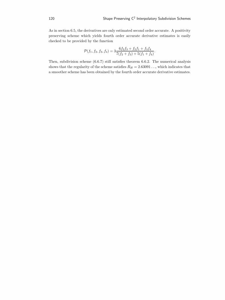
120 Shape Preserving C2 Interpolatory Subdivision Schemes
As in section 6.5, the derivatives are only estimated second order accurate. A positivitypreserving scheme which yields fourth order accurate derivative estimates is easilychecked to be provided by the function
P(f1, f2, f3, f4) = 36f2f3 + f2f1 + f3f4
7(f2 + f3) + 5(f1 + f4).
Then, subdivision scheme (6.6.7) still satisfies theorem 6.6.2. The numerical analysisshows that the regularity of the scheme satisfies RH = 2.63091 . . ., which indicates thata smoother scheme has been obtained by the fourth order accurate derivative estimates.

Chapter 7
Hermite-Interpolatory SubdivisionSchemes
7.1 Introduction
In this chapter we examine stationary interpolatory subdivision schemes for Hermitedata that consist of function values and first derivatives (see chapter 2). These schemesare attractive, as they allow to increase the smoothness using the same number of datapoints. A general class of Hermite-interpolatory subdivision schemes is proposed, andsome of its basic properties are stated. The goal is to characterise and construct certainclasses of nonlinear (and linear) Hermite-interpolatory subdivision schemes. Conditionsknown from the literature which are necessary and sufficient for smoothness of linearsubdivision schemes are discussed. For nonlinear Hermite-interpolatory subdivisionschemes these conditions are posed as assumptions in order to decrease the complexityof the construction of suitable schemes. Indeed, the number of possible nonlinearschemes is much larger than for linear subdivision schemes.The second part of this chapter, see section 7.3, deals with linear Hermite-interpolatorysubdivision schemes. The research contributes to the construction of Hermite schemesthat satisfy sufficient conditions for C2-convergence. This leads to larger classes ofC2 schemes than known from the literature. Section 7.4 focusses on shape preserv-ing Hermite-interpolatory subdivision. Some convexity preserving subdivision schemeswhich are rational and converge to at least C1 limit functions are presented.Hermite-interpolatory subdivision, or shortly Hermite subdivision, has been examinedin literature. In [Mer92], two-point Hermite schemes that lead to C1 functions in gen-eral, are discussed. Generalisations to Hermite subdivision for surfaces are proposedby [Mer94] and [vD97]. Stationary Hermite-interpolatory subdivision schemes are dis-cussed and characterised in [DL95,DL97], and the approach in this chapter follows the

122 7 Hermite-Interpolatory Subdivision Schemes
lines of these papers.Bounds on the regularity of specific classes of Hermite subdivision schemes are obtainednumerically in [YDL98]. In section 6.4, we proposed a simple numerical validationmethodology for analysing the smoothness of general (nonlinear) subdivision schemes.We use this numerical approach to investigate the smoothness of the Hermite schemesdiscussed in this chapter.The line of thought in the research in this chapter is partly obtained from rational inter-polation. A rational Hermite interpolant has been presented in [DG85b, Del89] whichis C1 and convex if the data are convex. This rational interpolant straightforwardlydefines a convexity preserving Hermite-interpolatory subdivision scheme: simply eval-uate the function value and the first derivative of the rational spline at the midpointsbetween the given data. The scheme, which obviously is C1, then becomes
f(k+1)2i = f
(k)i ,
f(k+1)2i+1 =
12
(f
(k)i + f
(k)i+1
)− 1
2h(k) 1
1∆f(k)
i −g(k)i
+ 1g
(k)i+1−∆f(k)
i
,
g(k+1)2i = g
(k)i ,
g(k+1)2i+1 = ∆f (k)
i −(∆f (k)
i − g(k)i )(g(k)
i+1 −∆f (k)i )(g(k)
i − 2∆f (k)i + g
(k)i+1)
(g(k)i+1 − g
(k)i )2
.
(7.1.1)
The aim of this chapter is to characterise a more general class of shape preservingHermite-interpolatory subdivision schemes, and to obtain more linear smooth (e.g., C2)subdivision schemes than known from the literature.
7.2 Hermite-interpolatory subdivision schemes
In this section, we set up the construction and characterisation for interpolatory subdi-vision schemes for Hermite data. We restrict ourselves to univariate Hermite data thatconsists of function values and derivatives at parameter values. In definition 2.1.2, thedefinition of an Hermite data set Φii is given. The definition of Hermite-interpolatorysubdivision schemes for Hermite data is as follows:
Definition 7.2.1 (Hermite-interpolatory subdivision schemes) The general Hermite-interpolatory subdivision scheme for the Hermite data points
Φ(k)i = (x(k)
i , f(k)i , g
(k)i ), (7.2.1)

7.2 Hermite-interpolatory subdivision schemes 123
where the parameter values x(k)i are equidistantly distributed, i.e., x(k)
i = 2−kih, isdefined by:
Φ(k+1)2i = Φ(k)
i ,
Φ(k+1)2i+1 = FΦ(Φ(k)).
(7.2.2)
The function FΦ is called the subdivision function.
This chapter deals with the problem of finding suitable functions FΦ, and one of theaims is to obtain a certain degree of smoothness:
Definition 7.2.2 (Smoothness) A stationary Hermite-interpolatory subdivision scheme(7.2.2) is said to be C`, ` ≥ 1, if the limit function f (∞) is ` times continuously differ-entiable and satisfies f (∞)(x(k)
i ) = f(k)i and f (∞)′(x(k)
i ) = g(k)i , ∀i, k.
Remark 7.2.3 Note that Hermite subdivision schemes are a special class of vector sub-division schemes, see e.g., [MS97,JRZ98,HJ98]. ♦
A starting point for the analysis of Hermite subdivision schemes is provided by [DL95]and [DL97], in which linear Hermite-interpolatory schemes are discussed and analysed.In this chapter, some of the definitions and notations are slightly generalised such thatthe characterisations and constructions are valid for nonlinear schemes as well: weconsider functions FΦ that may be nonlinear in their arguments.A general class of Hermite-interpolatory subdivision schemes is now introduced that hasthe following properties: the schemes are interpolatory, stationary, local, and possessthe usual natural symmetry conditions.
Definition 7.2.4 (General class of Hermite schemes) The general class of Hermitesubdivision schemes, for equidistant data with x
(k)i = 2−kih, i.e., h(k) = x
(k)i+1 − x
(k)i =
2−kh, is written as:
f(k+1)2i = f
(k)i ,
f(k+1)2i+1 =
12
(f
(k)i + f
(k)i+1
)− h(k) C1(∆f (k)
i , . . .),
g(k+1)2i = g
(k)i ,
g(k+1)2i+1 = ∆f (k)
i +M1(∆f (k)i , . . .),
(7.2.3)
The functions C1 as well asM1 are assumed to be chosen from the following collection:
F(∆f (k)i ), F(∆f (k)
i , g(k)i , g
(k)i+1), F(∆f (k)
i , g(k)i , g
(k)i+1,∆f
(k)i−1,∆f
(k)i+1), etc..

124 7 Hermite-Interpolatory Subdivision Schemes
The Hermite schemes are assumed to satisfy the usual symmetry conditions, see chapter3 and 4. Of course, the actual choice for the functions C1 andM1 influences the localityof the subdivision method.
Hermite subdivision schemes that make use of derivatives up to order ` are assumed togenerate limit functions which are at least C`. Therefore, in this chapter we are onlyinterested in schemes that are at least C1: a simple example is given by the choiceC1 = 0 and M1 = 0. This scheme generates the piecewise linear interpolant to theinitial data. The limit function is not C1 in the initial data points x(0)
i in general, sothis is not a Hermite scheme.
It is shown in [DL95] that the following quantities u(k)j are convenient for the smoothness
analysis of Hermite-interpolatory subdivision schemes that contain function values andfirst derivatives:
u(k)2i = g
(k)i and u
(k)2i+1 = ∆f (k)
i . (7.2.4)
The u(k)2i+j are attached at the parameters x(k+1)
2i+j and stand for derivative and deriva-tive estimate information, respectively. The continuous function u(k) is defined as thepiecewise linear interpolant to these data points (x(k+1)
2i+j , u(k)2i+j).
The following theorems are valid for linear Hermite-interpolatory subdivision schemes[DGL91,DL95,DL97]:
Theorem 7.2.5 A linear Hermite subdivision scheme generates C` (` ≥ 1) limit func-tions, only if it is exact for polynomials of degree `.
Theorem 7.2.6 If a linear Hermite subdivision scheme in the class (7.2.2) reproducesconstants, then there exists a scalar stationary subdivision scheme in which only quan-tities u(k)
i are involved, i.e.,
u(k+1) = Fu(u(k)). (7.2.5)
Furthermore, scheme (7.2.2) is C1 if and only if scheme (7.2.5) is C0. Then thelimit u(∞) generated by the scheme (7.2.5) is the derivative of the limit function f (∞)
generated by the scheme (7.2.2).
In fact, according to theorem 7.2.5 and 7.2.6, it has to be proved for C1-smoothness ofthe Hermite-interpolatory subdivision scheme that u(k) converges. The limit functionu(∞) then equals the derivative of f (∞).
Subdivision scheme (7.2.3) can be rewritten to a scheme in u(k)i as follows: the first
divided differences ∆f (k+1)2i and ∆f (k+1)
2i+1 are easily calculated, and subdivision scheme

7.2 Hermite-interpolatory subdivision schemes 125
(7.2.3) is completely characterised by:
g(k+1)2i = g
(k)i ,
∆f (k+1)2i = ∆f (k)
i − 2C1(∆f (k)i , . . .),
g(k+1)2i+1 = ∆f (k)
i +M1(∆f (k)i , . . .),
∆f (k+1)2i+1 = ∆f (k)
i + 2C1(∆f (k)i , . . .),
(7.2.6)
which is transformed to the derivative quantities u(k)2i+j :
u(k+1)4i = u
(k)2i ,
u(k+1)4i+1 = u
(k)2i+1 − 2C1(u(k)
2i+jj),
u(k+1)4i+2 = u
(k)2i+1 +M1(u(k)
2i+jj),
u(k+1)4i+3 = u
(k)2i+1 + 2C1(u(k)
2i+jj).
(7.2.7)
This is the reason why we restricted to the class of schemes (7.2.3): indeed (7.2.3) canbe rewritten to a subdivision scheme in u
(k)i , see (7.2.5).
Suitable quantities for the smoothness analysis of Hermite-interpolatory subdivisionschemes are provided by the notion of Hermite divided differences. The `-th divideddifferences ∆`u
(k)2i+j in the Hermite data u
(k)i are defined in [DL95, DL97]. For the
purpose of this chapter, the first and second Hermite divided differences in u(k)2i+j are
explicitly given:
∆u(k)2i =
u(k)2i+1 − u
(k)2i
x(k)i+1 − x
(k)i
=∆f (k)
i − g(k)i
h(k) ,
∆u(k)2i+1 =
u(k)2i+2 − u
(k)2i+1
x(k)i+1 − x
(k)i
=g
(k)i+1 −∆f (k)
i
h(k) ,
∆2u(k)2i =
∆u(k)2i −∆u(k)
2i−1
x(k)i+1 − x
(k)i−1
=∆f (k)
i − 2g(k)i + ∆f (k)
i−1
2(h(k))2
∆2u(k)2i+1 =
∆u(k)2i+1 −∆u(k)
2i
x(k)i+1 − x
(k)i
=g
(k)i+1 − 2∆f (k)
i + g(k)i
(h(k))2 .
The following theorem holds [DL95]:

126 7 Hermite-Interpolatory Subdivision Schemes
Theorem 7.2.7 (Convergence of Hermite subdivision) A linear Hermite subdivisionscheme (7.2.2) converges to a C` (` ≥ 1) function, if and only if a subdivision schemefor the differences ∆`−1u
(k)i exists, and moreover this scheme converges.
Remark 7.2.8 Observe that the Hermite divided differences are related to derivativesby
limk→∞
∆`−1u(k)i ≈
1`!f (`)(x(k)
i ).
Most of the results concerning subdivision schemes have only been proved for linearschemes. Since one of the goals in this chapter is to construct nonlinear shape preservingsubdivision schemes, the following assumptions are reasonable (see assumption 2.4.6,theorem 7.2.5 and 7.2.7):
Assumption 7.2.9 (Nonlinear subdivision) A nonlinear Hermite-interpolatory subdi-vision scheme is C`, only if:
1. the scheme for the `-th differences ∆`−1u(k)i exists.
2. the scheme for the `-th differences ∆`−1u(k)i reproduces constants, i.e., the scheme
reproduces polynomials of degree `.
3. the scheme for the `-th differences d(∆`−1u(k)i ) exists, and it is contractive.
The second condition has not been proved to be necessary for nonlinear subdivisionschemes. However, we were not able to construct a C` subdivision scheme that did notreproduce polynomials of degree `.
In order to construct schemes that generate C1 limit functions, condition 2 in as-sumption 7.2.9 yields that the Hermite-interpolatory subdivision scheme (7.2.5) mustreproduce linear polynomials. Reproduction of linear polynomials yields that C1 andM1 must satisfy
C1(u, u, u, . . .) = 0 and M1(u, u, u, . . .) = 0. (7.2.8)
The scheme for u(k)i exists, but it must be proved that this scheme converges, see
condition 2 in assumption 7.2.9. According to condition 3 of this assumption, thescheme for the Hermite differences
du(k)i = u
(k)i+1 − u
(k)i , (7.2.9)
must exist, and moreover this scheme must be contractive.For nonlinear subdivision schemes however, this scheme for the differences du(k)
i doesnot exist in general. We restrict to subdivision schemes in the class (7.2.3) for which

7.2 Hermite-interpolatory subdivision schemes 127
the difference scheme in du(k)i exists, see condition 3 in assumption 7.2.9. The scheme
for the Hermite differences du(k)i exists, if the functions C1 and M1 only depend on
du(k)2i+j . So, C and M are notated as C(du(k)
2i+jj) and M(du(k)2i+j) which are now
restricted to one of the following:
0, F(du(k)2i , du
(k)2i+1), F(du(k)
2i , du(k)2i+1, du
(k)2i−1, du
(k)2i+2), etc..
The scheme for the Hermite differences du(k)j is then as follows:
du(k+1)4i = du
(k)2i − 2C(du(k)
2i+jj),
du(k+1)4i+1 = 2C(du(k)
2i+jj) +M(du(k)2i+jj),
du(k+1)4i+2 = 2C(du(k)
2i+jj)−M(du(k)2i+jj),
du(k+1)4i+3 = du
(k)2i+1 − 2C(du(k)
2i+jj),
(7.2.10)
which automatically reproduces linear functions.
C2-convergence. For convergence to C2 limit functions of linear subdivision schemes,it is necessary that the scheme reproduces quadratic polynomials. This means thatthe scheme for the differences ∆u(k)
2i+j has to reproduce constants. Using the fact thatthe functions C andM are homogeneous of order 1 in their arguments, this scheme iseasily derived from (7.2.10):
∆u(k+1)4i = 2∆u(k)
2i − 4C(∆u(k)2i+jj),
∆u(k+1)4i+1 = 4C(∆u(k)
2i+jj) + 2M(∆u(k)2i+jj),
∆u(k+1)4i+2 = 4C(∆u(k)
2i+jj)− 2M(∆u(k)2i+jj),
∆u(k+1)4i+3 = 2∆u(k)
2i+1 − 4C(∆u(k)2i+jj).
(7.2.11)
The conditions on C and M for quadratic reproduction straightforwardly follow from(7.2.11): A = 2A− 4C(A,A, . . . , A) and A = 4C(A,A, . . . , A)± 2M(A,A, . . . , A), andhence
C(A,A, . . . , A) =14A and M(A,A, . . . , A) = 0. (7.2.12)
According to theorem 2.4.3, it is necessary and sufficient for C2-convergence of linearHermite-interpolatory subdivision schemes that the scheme for the differences d(∆u(k)
j )is contractive.

128 7 Hermite-Interpolatory Subdivision Schemes
To simplify the future analysis, we introduce the quantities v(k)2i+j :
v(k)2i =
12
(∆u(k)2i −∆u(k)
2i−1) and v(k)2i+1 = ∆u(k)
2i+1 −∆u(k)2i . (7.2.13)
The differences du(k)j and ∆u(k)
j are related by: du(k)2i+j = h(k)∆u(k)
2i+j .
The quantities v(k)2i+j are related to d(∆u(k)
2i+j) by
v(k)2i = 2d(∆u(k)
2i ) = h(k)∆2u(k)2i and v
(k)2i+1 = d(∆u(k)
2i+1) = h(k)∆2u(k)2i+1,
and as the quantities v(k)2i+j are defined by a simple linear combination of d(∆u(k)
2i+j), itis easily obtained that:
‖v‖∞ ≤ ‖d(∆u)‖∞, and ‖d(∆u)‖∞ ≤ 2‖v‖∞.
Therefore the following simple theorem is valid:
Theorem 7.2.10 The scheme for the differences v(k)i is contractive, if and only if the
scheme for the differences d(∆u(k)i ) is contractive.
For application of theorem 7.2.10, the scheme for v(k)i is required. For linear subdivision,
the scheme for v(k)j automatically exists if the scheme reproduces quadratic polynomials,
see section 7.3. For nonlinear schemes, this is a severe restriction: assumption 7.2.9must be valid.
C3-convergence. For the analysis of C3-smoothness of Hermite subdivision schemes,we define the quantities w(k)
2i+j :
w(k)2i+j := d(∆2u
(k)2i+j) = ∆2u
(k)2i+j+1 −∆2u
(k)2i+j = 3h(k)∆3u
(k)2i+j .
The third condition in assumption 7.2.9 yields that the scheme w(k)2i+j must exist, and
that it must be contractive in order to arrive at C3 Hermite schemes.
In the next section, the investigations on Hermite subdivision are continued with linearHermite schemes. Convexity preserving Hermite schemes are examined in section 7.4,
7.3 Linear Hermite-interpolatory subdivision schemes
In this section, we examine linear Hermite subdivision schemes in the class (7.2.3). Ascheme is called linear if the functions C andM are linear in their arguments.In [DL95,DL97], some general theory is provided for Hermite-interpolatory subdivisionschemes. The smoothness properties of Hermite subdivision schemes that have maximalapproximation order are examined in [YDL98].

7.3 Linear Hermite-interpolatory subdivision schemes 129
Two-point Hermite-interpolatory subdivision schemes have been examined in [Mer92],and a subclass of these schemes has been proved to be C1, which is also shown in thefollowing section:
Example 7.3.1 (Two-point Hermite subdivision) Linear two-point Hermite-interpol-atory subdivision schemes that satisfy the symmetry conditions and necessary condi-tions for C1 can be characterised generally by (7.2.10) and
C(du(k)2i+jj) = a1(du(k)
2i + du(k)2i+1) and M(du(k)
2i+jj) = b1(du(k)2i − du
(k)2i+1).
The class of two-point Hermite scheme is exact for quadratic polynomials if a1 = 1/8.Cubic polynomials are reproduced when additionally b1 = 1/4.
Necessary and sufficient for C1-convergence of this scheme is that the scheme for theHermite differences du(k)
2i+j is contractive. The scheme for the differences is:
du(k+1)4i = (1− 2a1)du(k)
2i − 2a1du(k)2i+1,
du(k+1)4i+1 = (2a1 + b1)du(k)
2i + (2a1 − b1)du(k)2i+1,
du(k+1)4i+2 = (2a1 − b1)du(k)
2i + (2a1 + b1)du(k)2i+1,
du(k+1)4i+3 = −2a1du
(k)2i + (1− 2a1)du(k)
2i+1.
(7.3.1)
For contractivity of du(k)2i+j it is sufficient that for all k: maxj |du(k+1)
j | ≤ λmaxj |du(k)j |,
with λ < 1. This single step condition, which provides estimates that are only sufficientand not necessary, can not be satisfied, since |1− 2a1|+ 2|a1| ≥ 1, for all a1 ∈ IR.The first four relevant equations of the double iteration difference scheme are
du(k+2)8i = (1− 4a1 − 2a1b1)du(k)
2i + 2a1(b1 − 1)du(k)2i+1,
du(k+2)8i+1 = (1− b1)(2a1 + b1)du(k)
2i + b1(b1 − 6a1)du(k)2i+1,
du(k+2)8i+2 = (2a1 + 6a1b1 − b1 + b21)du(k)
2i + b1(2a1 − b1)du(k)2i+1,
du(k+2)8i+3 = b1(1− 2a1)du(k)
2i + (2a1 + 2a1b1 − b1)du(k)2i+1,
(7.3.2)
and the other four equations follow from symmetry, see (7.3.1).It is easily seen from (7.3.2) that C1 schemes do exist in this class of two-point schemes:e.g., take b1 = 0, then the range 0 < a1 < 1/6 is sufficient for contractivity. In thecase a1 = 1/8, it can be derived that −1/2 < b1 < 3/4 is sufficient for C1. Finally, ifa1 = 1/8 and b1 = 1/4, the scheme reproduces cubic polynomials and is C1. ♦

130 7 Hermite-Interpolatory Subdivision Schemes
The section is continued with the construction of linear C2 Hermite-interpolatory subdi-vision schemes. A class of six-point schemes that satisfies natural symmetry conditions,and the necessary condition for C1 (reproduction of linear polynomials) is given by thedifference scheme (7.2.10) with C(du(k)
2i+jj) and M(du(k)2i+jj) given by
C(x1, x2, x3, x4, x5, x6, x7, x8, x9, x10) = a1(x1 + x2)
− a2(x3 + x4)− a3(x5 + x6)− a4(x7 + x8) + a5(x9 + x10) (7.3.3)
M(x1, x2, x3, x4, x5, x6, x7, x8, x9, x10) = −b1(x2 − x1)
+ b2(x4 − x3)− b3(x6 − x5) + b4(x8 − x7)− b5(x10 − x9). (7.3.4)
This scheme indeed depends on 10 variables, as differences in 6 derivatives g(k)i and 6-1
differences ∆f (k)i are taken into account. Four-point schemes are easily obtained by
restricting the coefficients to aj = 0, bj = 0, j = 4, 5.First, statements on the reproduction of certain classes of polynomials and the existenceof difference schemes are given:
Theorem 7.3.2 (Polynomial reproduction) The linear Hermite-interpolatory subdivi-sion scheme (7.2.10) with C and M given in (7.3.3) and (7.3.4) is exact for quadraticpolynomials if
a1 =18
+ a2 + a3 + a4 − a5, (7.3.5)
Moreover, if also
b1 =14
+ 5b2 − 7b3 + 11b4 − 13b5, (7.3.6)
the scheme reproduces cubic polynomials.If the coefficients satisfy (7.3.5), (7.3.6) and
a2 =1
128− 2a3 − 5a4 + 7a5, (7.3.7)
then quartic polynomials are reproduced.
Theorem 7.3.3 (Polynomial reproduction) Consider a linear Hermite-interpolatorysubdivision scheme in the class (7.2.3).Then the scheme reproduces polynomials of degree 1,2,3,4, respectively, if and only if(7.2.3) can be rewritten to a scheme in du(k)
j , v(k)j , w(k)
j (and dv(k)j ), dw(k)
j , respectively.
Construction. The treatment of six-point Hermite-interpolatory subdivision schemesis continued with the construction of schemes that generate C2 limit functions.Explicit subdivision schemes are constructed as follows: Consider the subdivisionscheme called F`1`2G`3`4 . The function value f (k+1)
2i+1 is determined by the Hermite-interpolating polynomial of degree 2`1 +2`2 through 2`1 successive function values f (k)
j

7.3 Linear Hermite-interpolatory subdivision schemes 131
and 2`2 successive derivatives. This polynomial is evaluated at the parameter valuex
(k+1)2i+1 , which defines the subdivision function value f (k+1)
2i+1 . For example, the schemeF21 is determined by the polynomial of degree six that interpolates the data points(x(k)i , f
(k)i , g
(k)i ), (x(k)
i+1, f(k)i+1, g
(k)i+1), (x(k)
i−1, f(k)i−1) and (x(k)
i+2, f(k)i+2). The derivatives g(k+1)
2i+1
are defined similarly by G`3`4 .
All subdivision schemes that are obtained in this way define a specific combination ofthe parameters aj and bj in (7.3.3) and (7.3.4), j = 1, 2, 3. For several schemes, thecoefficients are given in table 7.1. The integer in the last column indicates the degreeof the polynomials that are reproduced by the schemes.
F`1`2 a1 a2 a3 G`3`4 b1 b2 b3
F1118 0 0 3 G11
14 0 0 2
F2117128
1128 0 5 G21
53192
1192 0 4
F1225192
1384
1384 5 G12
47176
1704 - 1
704 4
F2271512
5256 - 3
512 5 G2277256
164
1256 4
Table 7.1: The coefficients aj and bj , j = 1, . . . , 3 for several schemes
Smoothness analysis. For analysing C2 Hermite-interpolatory subdivision schemes,we distinguish two approaches. The first approach is an analytical method for whichconvergence of suitable quantities is examined in an algebraic way. The expressionshowever, become more involved in general, and therefore a numerical method is attrac-tive. However, a numerical approach like in section 6.4 does not prove smoothness ofsubdivision schemes, since the limit iterations cannot performed.
We propose strategies for proving C2-convergence in an analytical way. In theorem7.2.10 it is shown that contractivity of the scheme for v(k)
2i+j , defined in (7.2.13), issufficient for C2-convergence. For many schemes, for which it is later proved that theyare C2, it empirically turns out to be impossible to show contractivity of v(k)
2i+j in a
single step strategy by examining v(k+1)4i+j , or even by double step estimates concerning
v(k+2)8i+j . Note that a single step estimate is also impossible for proving C1-convergence
of the linear four-point scheme, see [DGL87]. Therefore, it is required to define moresuited quantities.
One method for proving convergence to C2 limit functions is obtained as follows. Werestrict ourselves to subdivision schemes that reproduce cubic polynomials. Then the

132 7 Hermite-Interpolatory Subdivision Schemes
quantities v(k+1)4i+j can be written as
v(k+1)4i+j =
12v
(k)2i +
∑`
Aj,`dv(k)2i+`.
When also cubic polynomials are reproduced, i.e., the coefficients aj and bj satisfy(7.3.5) and (7.3.6), the scheme for dv(k)
2i+j exists, according to theorem 7.3.2.The advantage of this approach is that it is directly seen that contractivity of thescheme for dv(k)
2i+j is sufficient for C2-convergence. It appears that smoothness often
can be proved by examining dv(k+1)4i+j , j = 0, . . . , 3, i.e., by a single step strategy. The
contractivity factor λdv is defined by
maxj|dv(k+1)
4i+j | ≤ λdv maxj|dv(k)
2i+j |.
If this scheme for dv(k)2i+j has contractivity factor λdv < 1, we arrive at
maxj|v(k+1)
4i+j | ≤12|v(k)
2i |+Aλkdv,
and the condition λdv < 1 is indeed sufficient for contractivity of the quantities v(k)2i+j .
For several Hermite-interpolatory subdivision schemes, table 7.2 shows the analyticalresults for different contractivity factors.
Remark 7.3.4 All schemes treated in table 7.2 have also been compared with thesmoothness results from numerical experiments. It is known from the literature,e.g., [YDL98], that the scheme F11G11 is only C1. Furthermore, the schemes F22G22,F33G33 and F44G44 are known to be (at least) C2. According to the numerical ap-proach from section 6.4, many of the upper bounds on the Holder regularity of Hermiteschemes in [YDL98] turn out to be sharp: e.g., we obtained that the regularity of theHermite scheme F33G33 is RH ≈ 3.6173. ♦
Maximal C2-contractivity. The following construction for C2 Hermite schemes ex-ploits the relatively fast contractivity of the quantities dv(k)
2i+j . We restrict to Hermite-interpolatory subdivision schemes that are exact for cubic polynomials. Then thescheme for the differences dv(k)
2i+j exists. We now construct subdivision schemes suchthat the contractivity factor λdv is as small as possible for a single step strategy.Let us further restrict to four-point Hermite schemes. Since we require cubic exactness,and theorem 7.3.3 holds, four degrees of freedom are left: the coefficients a2, a3, b2 andb3.
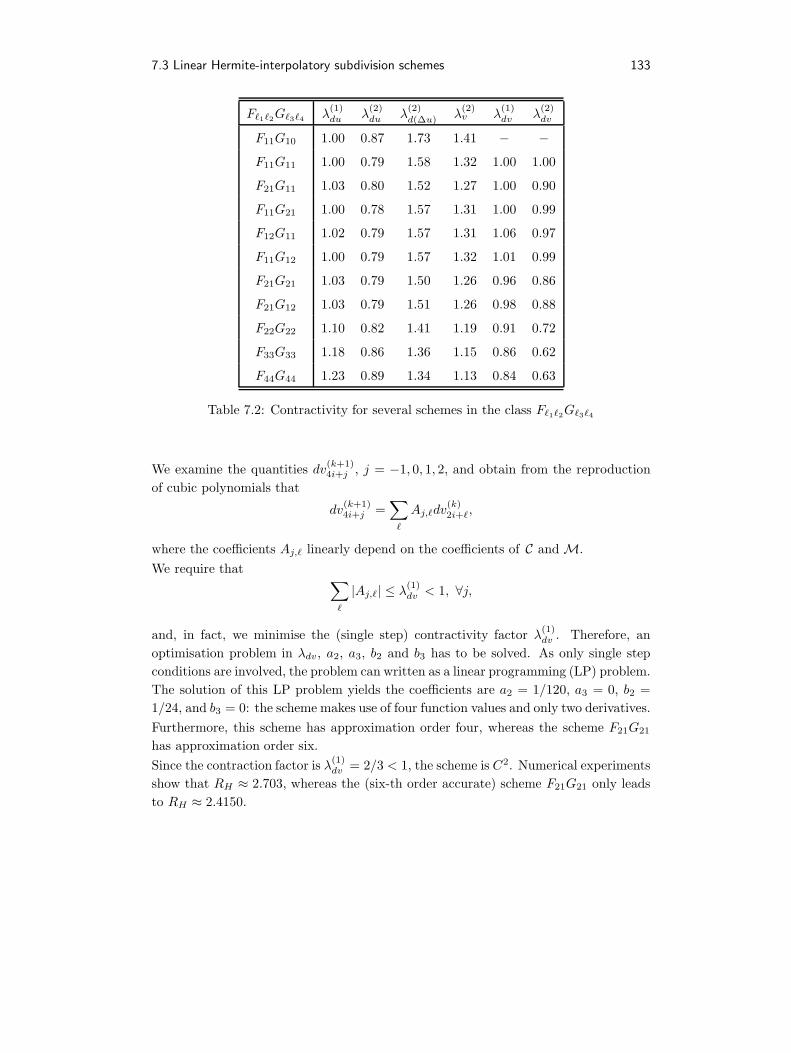
7.3 Linear Hermite-interpolatory subdivision schemes 133
F`1`2G`3`4 λ(1)du λ
(2)du λ
(2)d(∆u) λ
(2)v λ
(1)dv λ
(2)dv
F11G10 1.00 0.87 1.73 1.41 − −F11G11 1.00 0.79 1.58 1.32 1.00 1.00
F21G11 1.03 0.80 1.52 1.27 1.00 0.90
F11G21 1.00 0.78 1.57 1.31 1.00 0.99
F12G11 1.02 0.79 1.57 1.31 1.06 0.97
F11G12 1.00 0.79 1.57 1.32 1.01 0.99
F21G21 1.03 0.79 1.50 1.26 0.96 0.86
F21G12 1.03 0.79 1.51 1.26 0.98 0.88
F22G22 1.10 0.82 1.41 1.19 0.91 0.72
F33G33 1.18 0.86 1.36 1.15 0.86 0.62
F44G44 1.23 0.89 1.34 1.13 0.84 0.63
Table 7.2: Contractivity for several schemes in the class F`1`2G`3`4
We examine the quantities dv(k+1)4i+j , j = −1, 0, 1, 2, and obtain from the reproduction
of cubic polynomials that
dv(k+1)4i+j =
∑`
Aj,`dv(k)2i+`,
where the coefficients Aj,` linearly depend on the coefficients of C andM.We require that ∑
`
|Aj,`| ≤ λ(1)dv < 1, ∀j,
and, in fact, we minimise the (single step) contractivity factor λ(1)dv . Therefore, an
optimisation problem in λdv, a2, a3, b2 and b3 has to be solved. As only single stepconditions are involved, the problem can written as a linear programming (LP) problem.The solution of this LP problem yields the coefficients are a2 = 1/120, a3 = 0, b2 =1/24, and b3 = 0: the scheme makes use of four function values and only two derivatives.Furthermore, this scheme has approximation order four, whereas the scheme F21G21
has approximation order six.Since the contraction factor is λ(1)
dv = 2/3 < 1, the scheme is C2. Numerical experimentsshow that RH ≈ 2.703, whereas the (six-th order accurate) scheme F21G21 only leadsto RH ≈ 2.4150.
134 7 Hermite-Interpolatory Subdivision Schemes
Remark 7.3.5 The results for the smoothness of Hermite subdivision schemes areconsistent. Indeed, the numerically obtained values for α2, see section 6.4, satisfyα2 ≥ − log2(λ(k)
dv ), ∀k, and this lower bound on the smoothness tends to the numerialvalue of α2 as k tends to infinity. ♦
7.4 Convexity preserving Hermite-interpolatory subdivision schemes
In this section, Hermite-interpolatory subdivision schemes are examined that preserveconvexity. These schemes are necessarily nonlinear. First, a sufficient condition for con-vexity preservation is presented, and a sufficient condition for C1-convergence is pro-posed. Some convexity preserving Hermite-interpolatory subdivision schemes that gen-erate continuously differentiable limit functions are examined. Extensions to smootherconvexity preserving subdivision schemes are treated.The definition of convexity of a univariate Hermite data set is:
Definition 7.4.1 (Convexity of Hermite data) A Hermite data set (xi, fi, gi)i is saidto be (strictly) convex, if there exists a (strictly) convex function f that interpolates theHermite data, i.e., f(xi) = fi and f ′(xi) = gi, ∀i.
The following theorem provides a sufficient condition for convexity preservation:
Theorem 7.4.2 (Convexity preservation) A Hermite-interpolatory subdivision schemein the class (7.2.3) preserves convexity, if C and M satisfy
0 ≤ 12
∣∣∣M(du(k)2i+jj)
∣∣∣ ≤ C(du(k)2i+jj) ≤
12
mindu
(k)2i , du
(k)2i+1
. (7.4.1)
Furthermore, the scheme then converges and generates a continuous limit function.
Proof. Provided du(k)2i+j ≥ 0, ∀j, the condition du(k+1)
4i+j ≥ 0, ∀j is necessary for convexitypreservation. Hence, using (7.2.10), the following conditions are obtained:
C(du(k)2i+jj) ≤
12du
(k)2i , C(du(k)
2i+jj) ≥ −12M(du(k)
2i+jj),
C(du(k)2i+jj) ≥
12M(du(k)
2i+jj), C(du(k)2i+jj) ≤
12du
(k)2i+1,
and these conditions can be written as in (7.4.1).If the scheme preserves convexity, the (convex) piecewise linear interpolant f (k) to thedata points (x(k)
i , f(k)i ) can be constructed. The sequence of functions f (k) is bounded
and monotone decreasing, therefore the limit function f (∞) exists, and the scheme con-verges, see theorem 3.3.5.

7.4 Convexity preserving Hermite-interpolatory subdivision schemes 135
Next, a theorem concerning C1-convergence of convexity preserving Hermite subdivi-sion schemes is given:
Theorem 7.4.3 (C1-convergence) A convexity preserving Hermite-interpolatory sub-division scheme in the class (7.2.3) is C1, if the scheme for the differences du(k)
2i+j iscontractive.
Proof. The continuously differentiable function f (k) on the interval I(k)i := [x(k)
i , x(k)i+1] is
defined by the two-point rational Hermite interpolant to the data points (x(k)i , f
(k)i , g
(k)i )
and (x(k)i+1, f
(k)i+1, g
(k)i+1), see (2.2.13). The derivative of this function is called g(k) = f (k)′.
The subdivision scheme is known, see theorem 7.4.2, to converge, and all functionsf (k) are continuously differentiable by construction. Therefore, it is sufficient for C1-convergence that the sequence of functions g(k) converges. This is achieved when‖g(k+1) − g(k)‖∞ is contractive. As both g(k+1) and g(k) are monotone functions, thefollowing estimate is easily obtained:
‖g(k+1) − g(k)‖∞ = maxi
maxx∈I(k)
i
∣∣∣g(k+1)(x)− g(k)(x)∣∣∣ = max
i|g(k)i+1 − g
(k)i |
= maxi|g(k)i+1 −∆f (k)
i + ∆f (k)i − g(k)
i | = maxi|du(k)
2i+1 + du(k)2i |
≤ 2 maxjdu
(k)j ,
which shows that it is sufficient for C1-convergence of a convexity preserving Hermite-interpolatory subdivision scheme that the differences du(k)
2i+j are contractive.
Under relatively weak conditions on C and M, theorem 7.4.3 can be generalised for alarger class of subdivision schemes. The theorem holds for all linear schemes. In addi-tion, it holds for a larger class of nonlinear schemes, e.g., if C and M can be boundedas follows: C(du(k)
2i+jj) ≤ C1 maxdu(k)2i , du
(k)2i+1. This is the case for example if the
Hermite scheme preserves convexity.
Examples of convex schemes. Next, in the following theorems, two examples of rel-atively simple subdivision schemes that preserve convexity are given. The scheme intheorem 7.4.4 reproduces convexity preserving C1 rational splines [Del89], and it isobtained by defining the new function value and the new derivative using the convexitypreserving rational Hermite interpolant, see section 7.1.
Theorem 7.4.4 (The rational spline scheme) The Hermite-interpolatory subdivisionscheme (7.2.3) where C(du(k)
2i , du(k)2i+1) and M(du(k)
2i , du(k)2i+1) satisfy
C(x, y) =12
11x + 1
y
and M(x, y) =xy(x− y)(x+ y)2 , (7.4.2)

136 7 Hermite-Interpolatory Subdivision Schemes
preserves convexity. Furthermore, the limit function generated by this scheme is con-tinuously differentiable for any strictly convex initial Hermite data set.
Proof. Convexity is preserved as the functions C andM satisfy the sufficient conditionfor convexity in theorem 7.4.2:
M(x, y) =xy(x− y)(x+ y)2 =
xy
x+ y· x− yx+ y
≤ xy
x+ y= 2C(x, y).
Clearly, since this Hermite subdivision scheme reproduces C1 rational splines, thescheme is C1.
The second example provides a much simpler scheme which also generates C1 limitfunctions:
Theorem 7.4.5 The Hermite-interpolatory subdivision scheme (7.2.3) where the func-tions C(du(k)
2i , du(k)2i+1) and M(du(k)
2i , du(k)2i+1) satisfy
C(x, y) =12
11x + 1
y
and M(x, y) = 0, (7.4.3)
preserves convexity. Furthermore, the limit function generated by this scheme is con-tinuously differentiable for any strictly convex initial Hermite data set.
Proof. Convexity preservation is easily checked with theorem 7.4.2, since the choicesfor C and M satisfy condition (7.4.1).According theorem 7.4.3, contractivity of the scheme for du(k)
j is sufficient for C1-convergence.. After a simple calculation, using (7.2.10), the difference scheme becomes:
du(k+1)4i = du
(k)2i
du(k)2i
du(k)2i + du
(k)2i+1
= du(k)2i
q(k)i
1 + q(k)i
,
du(k+1)4i+1 = du
(k+1)4i+2 = du
(k)2i
du(k)2i+1
du(k)2i + du
(k)2i+1
= du(k)2i
1
1 + q(k)i
,
du(k+1)4i+3 = du
(k)2i+1
du(k)2i+1
du(k)2i + du
(k)2i+1
= du(k)2i+1
1
1 + q(k)i
,
(7.4.4)
where the ratios q(k)i are defined by
q(k)i =
du(k)2i
du(k)2i+1
. (7.4.5)

7.4 Convexity preserving Hermite-interpolatory subdivision schemes 137
The subdivision scheme for the ratios q(k)2i+j is:
q(k+1)2i =
du(k+1)4i
du(k+1)4i+1
=du
(k)2i
du(k)2i+1
= q(k)i and q
(k+1)2i+1 =
du(k+1)4i+2
du(k+1)4i+3
=du
(k)2i
du(k)2i+1
= q(k)i ,
which directly yields that q(k)2ki+j = q
(0)i , ∀j = 0, . . . , 2k − 1, and therefore
maxi,j
du(k+1)4i+j ≤ max
i
q(0)i
1 + q(0)i
·maxi,j
du(k)2i+j ,
and since the Hermite data are strictly convex, i.e., q(0)i /(1 + q
(0)i ) < 1, ∀i, this com-
pletes the proof.
Remark 7.4.6 It is easily checked that the simple scheme g(k+1)2i+1 = 1
2 (g(k)i + g
(k)i+1), does
not preserve convexity of the Hermite data in general.Indeed, the function M(du(k)
2i , du(k)2i+1) is given by M(x, y) = (y − x)/2, and it is not
possible to find a function C(du(k)2i , du
(k)2i+1) that satisfies convexity condition (7.4.1):
e.g., consider the case x ≤ y, then C has to satisfy (y− x)/2 ≤ C(x, y) ≤ x/2, which isnot satisfied for large y. ♦
A more general construction is the following: consider the class of schemes (7.2.3),and try to find bivariate functions C(x, y) andM(x, y) that satisfy convexity condition(7.4.1). We further restrict ourselves to methods that define the new function value by
C(x, y) =12
11x + 1
y
,
determined by the rational two-point Hermite interpolant that preserves convexity.Therefore, the condition for convexity, see (7.4.1), is
|M(x, y)| ≤ 11x + 1
y
.
Examples that satisfy this condition are the function M coming from the rational fitscheme, i.e.,M in (7.4.2), orM = 0. A more general choice is e.g.,
M(u, v) =xy(x− y)
`1(x2 + y2) + `2xy,
and requiring that the derivative is defined at least O(h3) yields that `2 = 4− 2`1, i.e.,
M(x, y) =xy(x− y)
`1(x2 + y2) + (4− 2`1)xy=
1`1x−yxy + 4xy
,

138 7 Hermite-Interpolatory Subdivision Schemes
and the condition `1 ≥ 1 is sufficient for convexity preservation. If `1 = 1, the rationalfit scheme is obtained.Shape preserving subdivision schemes that are only C1 have been proposed in thissection so far. This is due to our choice to keep restricted to two-point schemes.The presented schemes use only two function values and two derivatives. Hence thelimit function in an interval [x(k)
i , x(k)i+1] is only governed by f (k)
i , f (k)i+1, g(k)
i , and g(k)i+1.
And it is easily seen that the limit function is at most C1 in general. According to thesame arguments, a two-point Lagrange subdivision scheme cannot be C1 in general.Formulated more general, this leads to the following theorem:
Theorem 7.4.7 Consider a two-point Hermite-interpolatory subdivision scheme thatmakes use of function values and derivatives up to order `. Then the subdivision schemecannot generate limit functions that are C`+1, in general.
In the next section, we present some ad hoc approaches for obtaining schemes that arepossibly of higher order smoothness.
Construction of schemes of higher smoothness. The construction of convexity pre-serving Hermite subdivision schemes is continued with four-point schemes which mightlead to smoother limit functions.First, we restrict ourselves to the class of schemes (7.2.3) with
C(x, y) =12
11x + 1
y
,
determined by the rational two-point Hermite interpolant which preserves convexity.The motivation behind this restriction is the knowledge that there exists linear schemesin the class F11G`3`4 that generate C2 limit functions. These schemes also use the two-point Hermite-interpolating cubic fit for the new function value. Therefore, convexitypreserving subdivision schemes might exist for which f (k+1)
2i+1 is determined by only twopoints.We are looking for functionsM(du2i+jj) that satisfy convexity condition (7.4.1), i.e.,
|M(du2i+jj)| ≤1
1du2i
+ 1du2i+1
.
A simple idea is to apply a suitable four-point monotonicity preserving subdivisionscheme to four successive monotone data: the divided differences in the ’new’ data,i.e., a scheme like
g(k+1)2i+1 = FM (∆f (k+1)
2i−1 ,∆f (k+1)2i ,∆f (k+1)
2i+1 ,∆f (k+1)2i+2 ), (7.4.6)

7.4 Convexity preserving Hermite-interpolatory subdivision schemes 139
In chapter 4, a class of four-point interpolatory monotonicity preserving subdivisionschemes has been constructed. Indeed, such schemes (where G is given in e.g., (4.6.1))can be used for the successive differences:
g(k+1)2i+1 =
12
(∆f (k+1)
2i + ∆f (k+1)2i+1
)+
12
(∆f (k+1)2i+1 −∆f (k+1)
2i )G(q(k+1)2i , Q
(k+1)2i+1 ),
where the quotients q(k)j and Q
(k)j are defined in (2.1.10).
The divided differences ∆f (k+1)2i and ∆f (k+1)
2i+1 are given in (7.2.6), and satisfy
∆f (k+1)2i + ∆f (k+1)
2i+1 = 2∆f (k)i ,
∆f (k+1)2i+1 −∆f (k+1)
2i = 4C(du(k)2i , du
(k)2i+1) = 2
du(k)2i du
(k)2i+1
du(k)2i + du
(k)2i+1
,
which simplifies the scheme:
g(k+1)2i+1 = ∆f (k)
i +du
(k)2i du
(k)2i+1
du(k)2i + du
(k)2i+1
G(q(k+1)2i , Q
(k+1)2i+1 ).
It is easily checked that this produces a class of Hermite-interpolatory subdivisionschemes which preserve convexity. However, the algebraic expressions involved to proveeven C1 are too complicated. The smoothness analysis has therefore been performedby the numerical methodology presented in chapter 6, which yields that the resultingschemes are only C1. The derivatives in (7.4.6) are estimated more accurately, whenthe monotone scheme for the derivatives is restricted to `1 + 2`2 + `3 = 4. Then, thenumerically obtained smoothness is: α0 ≈ 1 and 0 < α1 < 1 for many data sets, whichagain does not lead to C2 limit functions.
The linear analogue of this construction is obtained by defining C by the cubic two-pointHermite interpolant, i.e., the linear scheme
f(k+1)2i+1 =
12
(f
(k)i + f
(k)i+1
)− 1
8
(g
(k)i+1 − g
(k)i
). (7.4.7)
The linear four-point scheme with w = 1/12 is used for FM in (7.4.6). This yields alinear scheme in the class (7.2.3), where the coefficients are defined by
a1 =18, a2 = 0, a3 = 0, b1 =
112, b2 = − 1
16, b3 = − 1
48.
However, this linear Hermite scheme is only C1, and therefore it is reasonable thata similar process for convex schemes, as sketched above, indeed does not lead to C2
subdivision schemes.

140 7 Hermite-Interpolatory Subdivision Schemes
The question arises whether there exists a four-point Hermite scheme based on (7.4.7)that can generate C2 limit functions. A two-step analysis shows that maximal con-tractivity of dv(k+2)
8i+j leads to a contractivity factor of λ(2)dv ≈ 0.8 < 1. Therefore, this
is a C2 Hermite scheme, which resulting coefficients are b3 = 0, b2 = 1/8−√
3/24 andb1 = 7/8− 5
√3/24. Since the schemes are linear and the contractivity factor is strictly
smaller than 1, there exists a larger class of linear Hermite-interpolatory subdivisionschemes that generate C2 functions.This short intermezzo dealing with linear Hermite subdivision shows that it is conceiv-able that an appropriate choice of `1, `2 and `3 in (4.6.1) leads to a convexity preservingHermite-interpolatory subdivision scheme that generates C2 limit functions.

Chapter 8
A Linear Approach to Shape PreservingSpline Approximation
8.1 Introduction
The problem of scattered data fitting under constraints is important in many applica-tions, and a large number of methods for solving this problem have been proposed inthe literature. Often, the problem can be posed as the following optimisation problem: min
d‖Ad− f‖ ,
s.t. C(d) ≥ b.(8.1.1)
The vector f contains the M given data values, and d is the vector containing theN unknowns, e.g., the spline coefficients. The matrix A is of dimension M × N ,and the elements of A are determined by the approximation method, e.g., a splineapproximation. Constraints are given by a multivariate function C and a known vectorb of dimension L. The inequality constraints are nonlinear in the unknowns, in general.An example of a problem that can be solved by an optimisation program as in (8.1.1)is convexity-preserving approximation of scattered bivariate data using tensor-productB-splines, as we will discuss in more detail in section 8.6.For practical reasons, it is attractive if the constraints in problem (8.1.1) are linear inthe unknowns, or if they can be suitably approximated by sufficient linear constraints.In that case we have a constraint matrix C of dimension L×N , and the optimisationproblem simplifies to: min
d‖Ad− f‖ ,
s.t. Cd ≥ b.(8.1.2)

142 8 A Linear Approach to Shape Preserving Spline Approximation
This chapter focusses on problem (8.1.2), and the following questions naturally arise:
1. concerning the objective function: which approximation method, i.e., which norm,should be chosen?
2. concerning the constraints: how to linearise the shape constraints?
When these two questions have been answered, the constrained approximation problemcan be solved. The goal is to approximate the data arbitrarily well, but this processgenerates only an approximation in general, therefore:
3. concerning convergence: can we give a sequence of approximants that come arbi-trarily close to an interpolant?
These three issues are subsequently discussed in this chapter, which is organised asfollows:
1. The first part of this chapter treats the choice of the approximation method, or morespecifically, suitable choices for the norm in the objective function of problem (8.1.2).Here, we assume that the constraints are linear in the unknowns, and that they admita feasible solution. Section 8.2 reviews some constrained `p-approximation methods.Approximation in the `2-norm, the `∞-norm and the `1-norm, respectively, are treated.Both constrained `∞-approximation and constrained `1-approximation can simply berewritten as linear programming (LP) problems. Dependent on the application at hand,the different `p-norms all have their advantages and drawbacks, which is illustrated bya simple univariate example using convex cubic B-splines.Section 8.3 presents a new class of constrained approximation methods. These methodsare constructed by considering the constrained `2-approximation problem by minimis-ing the `2-residuals in the `p-norm, p ≥ 1. We refer to those norms as `
′
p. When p = 1 orp =∞, this again leads to optimisation problems that can straightforwardly be rewrit-ten to an LP-problem. The advantage of this approach is that these `
′p algorithms turn
out to be attractive especially in case of a large number of data: the complexity ofthe LP-problem becomes much lower for `
′p than for `p-approximation. In addition,
numerical experiments show that the constrained `′
p-methods generate solutions thatare much closer to the solution of the constrained least-squares (`2) method than theconstrained `p-approximation solutions for p = 1 or p =∞ are.The reasons why we focus on methods that can be written as LP-problems are thefollowing. Firstly, various implementations of linear programming are available, evenpublic domain. These methods are often simplex-based, relatively cheap, fast, robustand accurate, especially when the number of constraints is high. Secondly, the matrixcontaining the constraints is sparse, i.e., it contains a lot of zeroes. For large-scale

8.2 Constrained `p-approximation methods 143
computations, solvers exist that are based on a sparse treatment of the objective func-tion and the constraints. These commercial LP-solvers can even handle millions ofconstraints. In section 8.5 it is shown that an accurate linearisation of the bivariateconvexity constraints for tensor-product B-splines results in a large number of linearconstraints.
2. The second part of the chapter deals with the linearisation of the constraints. We dis-cuss sufficient linear conditions for shape preservation, for example when dealing withapproximating data with B-splines. First, in section 8.4, the construction of sufficientlinear constraints for shape preservation of univariate B-splines is briefly discussed:sufficient conditions for positivity, monotonicity and convexity are presented, and theyare formulated as linear inequalities in the unknowns.For bivariate spline functions, sufficient conditions for preservation of positivity ormonotonicity are presented as linear inequalities in the unknowns. In contrast withpositivity and monotonicity, the conditions for convexity of a bivariate function arenonlinear in second derivatives of that function. Recently, in [CFP97], a linearisationof convexity conditions was proposed that is much better than that based on diagonaldominance of the Hessian matrix. Generalisations to weaker conditions, i.e., conditionsthat are sufficient and ’almost’ necessary, are given in [Jut97b, Jut97a]. A simpleinterpretation of these weaker conditions is given in section 8.5.3.
3. Finally, the third part of this chapter provides a methodology to obtain a shapepreserving approximation that almost interpolates the given data, i.e., a method thatprovides a solution satisfying an arbitrarily small error tolerance. A sequence of ap-proximations using tensor-product B-splines is constructed. Each approximation isobtained by calculating the solution of a linear programming problem on a given knotset. The knot set of the B-spline is refined after each iteration in a specific way, if theapproximation does not satisfy the required error tolerance. After a number of itera-tions, this sequence of approximations generates a tensor-product B-spline approximantthat satisfies the shape constraints and that approximates the given data sufficientlywell. Some comments are made on how to generate this sequence of approximations,such that convergence is guaranteed.
8.2 Constrained `p-approximation methods
In this section, problem (8.1.2) is discussed for approximation in the `p-norm.Several numerical experiments for constrained `p-approximation have been performed.A typical example is provided by data points drawn from the function f(x) = |x|on [−1, 1] and the approximant is chosen in the class of cubic B-splines. The spline

144 8 A Linear Approach to Shape Preserving Spline Approximation
approximant is required to be convex, but the restriction to this type of constraint isnot relevant for the comparison in this chapter.Subsequently, the given data and the cubic B-spline approximant are graphically dis-played for this illustrative example. In a separate figure, the difference of the splineapproximant with the given function is shown. The position of the knots on which theapproximations are based is indicated at the x-axis. Clearly the number of data pointsis much larger than the number of knots, i.e., we consider the case M N .The `2, `∞ and the `1-approximation methods are discussed in the next sections.
8.2.1 Constrained `2-approximation
Least squares approximation (p = 2) is the most well-known and widely-used methodfor approximation. The reason for this is that unconstrained `2-approximation leads tothe problem of solving an N ×N system of linear equations:
ATAd−AT f = 0. (8.2.1)
−1 0 10
0.1
0.2
0.3
0.4
0.5
0.6
0.7
Figure 8.1: Convex `2-approximation of data from |x|.
Efficient and accurate methods exist to solve this matrix equation, even in the case oflarge N . However, if the approximation problem is constrained, the solution of (8.2.1)in general is not feasible. The usual approach (in case of inequality conditions) is thento solve an optimisation problem consisting of a quadratic objective function subjectto linear constraints. Efficient implementations of solution methods for constrainedleast squares exist. However, these quadratic programming (QP) methods are morecomplicated than linear programming (LP) solvers, especially for large problems.

Constrained `p-approximation methods 145
−1 0 10
0.02
0.04
0.06
0.08
Figure 8.2: Difference between convex `2-approximation and |x|.
8.2.2 Constrained `∞-approximation
In case of the max-norm (p =∞), also called minimax-approximation, problem (8.1.2)can be transformed to a linear programming problem, in contrast with a QP-problemfor constrained `2-approximation. It is a well-known fact that these LP-problems canbe solved much faster and more efficient and accurate than QP-problems, especiallyfor large problems.The way to arrive at the LP-problem is as follows: in case of `∞-approximation, themaximum error is minimised, and the way to incorporate this in a LP-problem is todefine the maximum error to be the scalar r, and add this single variable r as anadditional unknown in the approximation problem:
min r,
s.t. Cd ≥ b,−r · 1 ≤ Ad− f ≤ r · 1,
(8.2.2)
where 1 is an M -vector in which all elements are equal to one. The constraint matrixconsists of L+ 2M linear inequalities in N + 1 unknowns.
8.2.3 Constrained `1-approximation
Another method is obtained by taking p = 1, and this norm is attractive if the datacontain a few extreme observations, since `1-approximation is less influenced by outliersthan e.g., least squares. It is shown that `1-approximation can also be transformed toan LP-problem. Instead of introducing one single slack-variable (the unknown r insection 8.2.2), two slack vectors v and w of dimension M are introduced, satisfying:
v − w = Ad− f, with v ≥ 0, w ≥ 0, (8.2.3)
where v represent the positive part of Ad − f and w the negative part. According to`1-norm approximation, the objective
M∑i=1
|vi − wi| , (8.2.4)

146 8 A Linear Approach to Shape Preserving Spline Approximation
−1 0 10
0.1
0.2
0.3
0.4
0.5
0.6
0.7
Figure 8.3: Convex `∞-approximation of data from |x|.
−1 0 10
0.02
0.04
0.06
0.08
Figure 8.4: Difference between convex `∞-approximation and |x|.
has to be minimised.A simple observation shows that it is always possible to take (8.2.3) with either vi = 0or wi = 0, ∀i: if vi = a > 0 and wi = b > 0 defines a solution of the LP-problem,then vi = a − mina, b and wi = b − mina, b also solves the LP-problem with thesame objective. The objective function in (8.2.4) now simplifies, and the LP-problemfor constrained `1-approximation becomes:
minM∑i=1
(vi + wi) ,
s.t. Cd ≥ b,Ad− v + w = f,
v ≥ 0, w ≥ 0.
(8.2.5)
This yields that the number of variables in this LP-problem is N+2M and the numberof linear constraints L+M .

Constrained `p-approximation methods 147
−1 0 10
0.1
0.2
0.3
0.4
0.5
0.6
0.7
Figure 8.5: Convex `1-approximation of data from |x|.
−1 0 10
0.02
0.04
0.06
0.08
Figure 8.6: Difference between convex `1-approximation and |x|.
8.2.4 Comparison of constrained `p-approximation methods
Three methods for constrained `p-approximation have briefly been discussed in theprevious sections: the cases p = 1, 2,∞. We briefly summarise their advantages anddrawbacks:`2-approximation is probably the most well-known method. The constrained approx-imation problem however, cannot be solved by solving a system of linear equations,but generates a linearly constrained quadratic programming (QP) problem. This in-creases the computational costs and leads to inaccuracies, especially in case of manydata points or a high dimensional spline space.`∞-approximation is the method that minimises the maximum error that occurs in theapproximation, and from a mathematical point of view, this is ’the best’. Max-normapproximation can be written as linear programming, but the method gives rise tothe well-known minimax-behaviour: the maximal error occurs with both positive andnegative sign at several locations of the approximation. For our later purposes, it turnsout that this behaviour is disadvantageous, see section 8.6.
148 8 A Linear Approach to Shape Preserving Spline Approximation
Also `1-approximation can be transformed to a linear programming problem. Approx-imation in the `1-norm does not suffer from the drawbacks of `2 (QP) or `∞ (minimaxbehaviour).Both linearly constrained `1 and `∞-approximation can be rewritten to linear program-ming problems. However, the computational complexity increases in case of a largenumber of data, i.e., if M becomes large. Then, the number of constraints increasessignificantly, and the LP-problem leads to large-scale problems.In the next section, the data are approximated by so-called `
′
p-methods. These ap-proximation methods can also be transformed to LP-problems and they are especiallysuited for large data sets.
Remark 8.2.1 (Sparse matrices) In case of e.g., spline approximation, each spline seg-ment is only governed by a relatively small number of coefficients, and the same holdsfor the linear shape constraints. Although this implies that the constraint matrix con-tains many zeroes, most standard implementations do not use this sparsity. However,when only nonzero elements are stored, this gives the opportunity of dealing with alarge number of constraints. For this purpose, there exist large-scale sparse LP-solvers,which can even handle millions of constraints. ♦
8.3 Linear methods for constrained ’least squares’
In this section two methods for constrained approximation are introduced that lead tosolutions that are closer to the constrained least squares solution. This turns out to beattractive as it gives an indication how to determine where knots have to be inserted.The methods can be solved by LP-problems, and the complexity is much lower than`1-approximation if the number of data is large.
8.3.1 Constrained `′
p-approximation
In case of unconstrained `2-approximation the N×N system of linear equations (8.2.1)has to be solved for the unknown d. For constrained least squares approximationhowever, the solution of this linear system does not satisfy the constraints in general.The idea of the construction in this section is to minimise the `2-residuals in the `p-norm. The method, we call it `
′
p-approximation, is defined as follows: mind
∥∥ATAd−AT f∥∥p, p ≥ 1,
s.t. Cd ≥ b,(8.3.1)
8.3 Linear methods for constrained ’least squares’ 149
It is now straightforward to pose the linear programming problems that arise from`′p-approximation for the cases p =∞ and p = 1.
The constrained `′
∞-approximation problem is solved by the following LP-problem:min r,
s.t. Cd ≥ b,−r · 1 ≤ ATAd−AT f ≤ r · 1,
(8.3.2)
and its complexity is partially characterised by the L+2N linear constraints and N+1unknowns.The LP-problem that solves constrained `
′
1-approximation becomes:
minM∑i=1
(vi + wi) ,
s.t. Cd ≥ b,ATAd− v + w = AT f,
v ≥ 0, w ≥ 0.
(8.3.3)
The number of constraints is L+N , and the number of unknowns is 3N .Observe that the complexity of the `
′
1 and `′
∞ method does not depend on the numberof data M . These methods are therefore especially suited for approximation of largedata sets and functions.The results obtained by the `
′
p-approximation methods are compared with the resultsin the `p-norm in the next section.
8.3.2 Comparison of constrained `′p- and `p-approximation
In this section, the performance of the `′
p-approximation methods is compared to resultsobtained by using the `p-approximation.An important advantage of the LP-problems resulting from `
′
p-approximation is thattheir complexity is much lower than `p-approximation in case of large data sets, i.e.,if M is large. For example, the number of constraints for `∞ is L + 2M , where`′∞-approximation results in L + 2N constraints. As a result, the constrained `
′p-
approximation methods are better for approximating functions from the point of com-plexity.Secondly, `
′
p-approximation is attractive, because various numerical experiments clearlydisplay the resemblance of `
′p solutions to the `2-solution. Again, we consider the typical
example from section 8.2. The difference between the spline approximants with thegiven function is shown for respectively the norms `∞, `
′
∞, `2, `′
1, and `1. It is clearly

150 8 A Linear Approach to Shape Preserving Spline Approximation
seen in figure 8.7 that the approximations `′
∞ and `′
1 more resemble least squares than`∞ or `1 do, which is natural from the construction.
−1 0 10
0.02
0.04
0.06
0.08
`∞
−1 0 10
0.02
0.04
0.06
0.08
`′
∞
−1 0 10
0.02
0.04
0.06
0.08
`2
−1 0 10
0.02
0.04
0.06
0.08
`′
1
−1 0 10
0.02
0.04
0.06
0.08
`1
Figure 8.7: Error of convex approximation of dense data from |x| on [−1, 1].
8.4 Linear constraints for shape preservation of univariate splines
In this section we discuss the construction of sufficient linear constraints for shapepreservation in case of univariate B-splines. The sufficient conditions can be formulatedas linear inequalities in the B-spline control points. Subsequently, sufficient linearconstraints for preservation of positivity, monotonicity and convexity are discussed.The generation of shape constraints is relatively simple in the univariate case. It isnecessary and sufficient for k-convexity of a univariate spline is that its k-th derivativeis nonnegative, see chapter 2. In case of B-splines of degree n, this k-th derivative can

8.4 Linear constraints for shape preservation of univariate splines 151
be written as a B-spline of degree n− k [dB78,Sch82,Far90]:
u(k)(x) =Nξ−1∑i=−n+k
d(k)i Nn−k
i (x), (8.4.1)
where the coefficients d(k)i are the B-spline coefficients of the k-th derivative of u, which
depend on di in a known way.A well-known result for B-splines is that non-negativity of the B-spline coefficientsyields a nonnegative B-spline, which straightforwardly follows from the convex-hullproperty of B-splines. The requirement that d(k)
i ≥ 0 is sufficient for k-convexity ofthe spline u(x). This generates a number of linear inequality constraints in the B-spline coefficients di. The Bezier polygon of a spline is known to be closer to the splinethan the B-spline control polygon, however. Non-negativity of the Bezier net is alsoa sufficient condition for non-negativity of a Bezier-Bernstein polynomial, see theorem2.2.2, and this condition on the Bezier points is therefore less restrictive for preservationof k-convexity than the conditions on the B-spline control points d(k)
i . Hence, the B-spline u(k) is converted into its Bezier-Bernstein formulation, and on every segment[ξi, ξi+1], the spline can be written as u(k)
i , see (2.2.4), based on the Bezier points saybi, i = 0, . . . , n − k. Theorem 2.2.2 yields that the spline segment u(k)
i is nonnegativeif the Bezier points bi are nonnegative. These conditions can straightforwardly berewritten to linear inequalities in the coefficients di of the B-spline u.
Necessity of the constraints. The restriction of the sufficient linear constraints canbe relaxed by degree elevation. According to (2.2.3), a spline segment u(k)
i can berepresented by n− k + 2 Bezier points b(1)
i instead of n− k + 1 Bezier points bi. TheBezier polygon b(1)
i i then lies in the convex hull of bii. A condition for k-convexityof u(k)
i is then that b(1)i ≥ 0, ∀i. After repeated degree raising, the Bezier net of u(k)
i
is known to converge to the spline u(k)i [dB78,Sch82,Far90]. As a result, the sufficient
conditions converge to the necessary and sufficient shape conditions, when the degreeof the representation of the spline tends to infinity. The degree of the spline u itself ofcourse does not change, but the number of linear inequalities in the B-spline controlpoints increases significantly.The degree of the B-spline has not to be raised globally: the degree of the spline canbe raised only in regions where the approximation is expected to have difficulties tosatisfy the constraints. In those regions, the linear inequalities in the LP-problem willbecome active, and additional degrees of freedom have to be introduced, e.g., by knotinsertion.In the bivariate case, the construction of linear constraints becomes much more in-volved. This is discussed in the next section.

152 8 A Linear Approach to Shape Preserving Spline Approximation
8.5 Linear constraints for shape preservation of bivariate splines
In this section, the construction of linearised shape constraints for bivariate functionsis discussed. Subsequently, positivity, monotonicity and convexity conditions are dis-cussed, and the conditions are applied to tensor-product B-splines.Again, as in the univariate case, the conditions for shape preservation are only sufficientand not necessary in general. However, the linear constraints become less restrictiveafter degree elevation, as the Bezier polygon is known to converge to the Bezier curve.When the degree of the spline is raised to a sufficiently high degree, the restrictionbecomes weaker and (almost) necessary.
8.5.1 Bivariate positivity constraints
In case of the construction of positivity constraints for bivariate tensor-product B-splines u(x, y) it is sufficient to convert the B-spline to the Bezier-Bernstein form.Sufficient positivity constraints are then obtained by requiring that Bezier points bi,jare nonnegative.
8.5.2 Bivariate monotonicity constraints
In this section, we discuss the construction of linear conditions which are sufficient formonotonicity preservation.The most frequently used condition for monotonicity reads
fx ≥ 0 and fy ≥ 0, ∀x, y, (8.5.1)
and this condition can straightforwardly be applied to tensor-product B-splines bydetermining the B-spline derivatives ux and uy. As has been done for the univariateshape conditions, sufficient linear constraints are obtained by converting the B-splineexpressions for both ux(x, y) and uy(x, y) to their Bezier-Bernstein form and requiringthat the corresponding Bezier nets of ux and uy are both non-negative.More general conditions for monotonicity of a multivariate function are presented indefinition 2.1.15, and the vectors γj determined the directions for which monotonicityis required. According to this definition, the condition for a bivariate continuouslydifferentiable function becomes γj · ∇f ≥ 0, ∀j, see (2.1.13), e.g., in the bivariate case
γ1,1fx + γ1,2fy ≥ 0 and γ2,1fx + γ2,2fy ≥ 0. (8.5.2)
Condition (8.5.1) is a special case of this condition, i.e., γj = ej , j = 1, 2.The sufficient monotonicity conditions (8.5.2) for a bivariate function f are appliedto tensor-product B-splines u(x, y) of degree nx × ny. The derivatives ux and uy are

8.5 Linear constraints for shape preservation of bivariate splines 153
converted into the Bezier-Bernstein form, and linear combinations of ux and uy haveto be calculated. To be able to algebraically calculate the sum of the Bezier-nets of uxand uy, both must be of the same degree. Since ux is of degree (nx − 1)× ny, and uyof degree nx × (ny − 1), the degree of ux as well as uy have to be raised to (at least)nx × ny. Then, the linear combinations in the inequalities (8.5.2) can be determined,and sufficient conditions for monotonicity are obtained by requiring that the Beziernets of both inequalities are nonnegative. Again, the resulting conditions are easilyconverted into linear inequalities in the B-spline control points.
8.5.3 Bivariate convexity constraints
Theorem 2.1.11 provides three conditions that are necessary and sufficient for convexityof a twice differentiable bivariate function f(x, y). However, the third condition isnonlinear in the second derivatives of the function f , and therefore when applied to aspline these conditions are also nonlinear in the control points:
fxx(x, y)fyy(x, y)− f2xy(x, y) ≥ 0. (8.5.3)
In this section, this convexity condition is linearised, and it is shown that the linearisedconstraints on f are sufficient for convexity of f . The conditions are then applied totensor-product splines.A simple condition on f that is sufficient for convexity is [Dah91]:
fxx(x, y) ≥ 0, fyy(x, y) ≥ 0, fxy(x, y) = 0, ∀x, y. (8.5.4)
It is easily verified that (8.5.4) indeed implies the three conditions in theorem 2.1.11.However, the class of surfaces that satisfy the condition fxy ≡ 0, a so-called transla-tional function, is known to be too restrictive for real applications: on a rectangulardomain for example, such a surface is fully described by two adjoining boundaries.The following linearisation of the convexity conditions has turned out to be useful forpractical purposes, and the conditions are less restrictive than (8.5.4). These conditionscan be interpreted as diagonal dominance of the Hessian matrix (2.1.12).
Theorem 8.5.1 (Linearisation of convexity conditions) A two times continuously dif-ferentiable function f : Ω ⊂ IR2 → IR is convex if
fxx(x, y) ≥ |fxy(x, y)| and fyy(x, y) ≥ |fxy(x, y)| , ∀(x, y) ∈ Ω. (8.5.5)
Proof. Since |fxy(x, y)| ≥ 0, the first and second condition in theorem 2.1.11 aresatisfied. The inequality
fxx(x, y)fyy(x, y)− f2xy(x, y) ≥ |fxy(x, y)|2 − f2
xy(x, y) = 0

154 8 A Linear Approach to Shape Preserving Spline Approximation
makes that the third condition is also satisfied.
The linear conditions (8.5.5) can be written into the following four inequalities in f
and its derivatives:
fxx + fxy ≥ 0, fxx − fxy ≥ 0, fyy + fxy ≥ 0 and fyy − fxy ≥ 0. (8.5.6)
Application to splines. The sufficient convexity conditions (8.5.6) for a bivariate func-tion f(x, y) are applied to tensor-product splines u(x, y). The degree of the bivariatespline is assumed to be nx × ny, and the relevant second derivative functions are uxx,uyy, and uxy. As an example, consider the first inequality from (8.5.6): uxx + uxy ≥ 0.Again, as in the univariate case, both B-splines uxx and uxy are converted to theBezier-Bernstein formulation. The degree of uxx as well as uxy has to be raised to atleast (nx − 1) × ny, to be able to algebraically calculate their sum. It is sufficient fornon-negativity of this inequality that its Bezier net is nonnegative, which is a weakercondition for shape preservation than non-negativity of the B-spline control net. Theconditions on the Bezier points are transformed back into linear inequalities in theB-spline coefficients. The other inequalities from (8.5.6) are treated similarly.
Complexity. An example shows that in general a large number of constraints is gen-erated by this approach for the construction of sufficient linear convexity constraints.For a nx×ny-degree B-spline based on the knot partitions ξ0, . . . , ξNξ and ψ0, . . . , ψNψ ,the number of inequalities becomes at least
L = Nξ ×Nψ × (2(nx − 1)ny + 2nx(ny − 1)) = 2NξNψ(2nxny − nx − ny).
In case of a relatively simple example of cubic tensor-product B-splines based on Nξ =Nψ = 20, the number of inequalities becomes L = 2 · 20 · 20(2 · 3 · 3 − 3 − 3) = 9600.Note that the complexity increases when the approximation is based on a denser knotset and the number of inequalities increases even more when the degree of the splinebecomes higher.
The following example shows that the sufficient linearised convexity conditions (8.5.5)are not necessary for convexity preservation:
Example 8.5.2 Consider the two times differentiable bivariate function
f(x, y) = 2x2 + xy +15y2.
This function is convex, since the (nonlinear) condition (8.5.3) holds:
4 ≥ 0,25≥ 0, 4 · 2
5− 12 =
35> 0.

8.5 Linear constraints for shape preservation of bivariate splines 155
The linearised conditions (8.5.5) however yield:
fxx = 4 ≥ 1 = |fxy| and fyy =256≥ 1 = |fxy|,
which suggests to improve the sufficient convexity conditions given by (8.5.5). ♦
Theorem 8.5.3 (Linearisation of convexity conditions) A two times continuously dif-ferentiable function f : Ω ⊂ IR2 → IR is convex if there exists a 0 < L < ∞, suchthat
fxx(x, y) ≥ L |fxy(x, y)| and fyy(x, y) ≥ 1L|fxy(x, y)| , ∀(x, y) ∈ Ω. (8.5.7)
Proof. Since L > 0, we obtain that the first and second condition in theorem 2.1.11are satisfied. The inequality
fxx(x, y)fyy(x, y)− f2xy(x, y) ≥ L |fxy(x, y)| 1
L|fxy(x, y)| − f2
xy(x, y) = 0,
makes that the third condition is also satisfied.
The case L = 1 in theorem 8.5.3 corresponds to the conditions in theorem 8.5.1. Ingeneral, this choice is not optimal and the question arises how to determine a betterchoice for L, which is required to satisfy (8.5.7):
|fxy(x, y)|fyy(x, y)
≤ L ≤ fxx(x, y)|fxy(x, y)| .
Note that L in theorem 8.5.3 can depend on (x, y). A local estimate for L can bedetermined for each subdomain of the spline: Ωi,j = (x, y)| ξi ≤ x ≤ ξi+1, ψi ≤ y ≤ψi+1, by calculating numbers ai,j , bi,j , and ci,j that approximate fxx, fyy and |fxy|on Ωi,j respectively by examining the data near Ωi,j . A local estimate for L is then forexample obtained by the arithmetic mean or geometric mean, i.e., :
Li,j =12
(ci,jbi,j
+ai,jci,j
)or Li,j =
2ci,jai,j
+ bi,jci,j
.
Weak linear convexity conditions. The construction of linear convexity constraintsis further simplified. The approach starts from the general convexity condition for abivariate function, and it also gives a simple graphical interpretation of the generalclass of linear constraints that is presented in [Jut97b].Define λ1 and λ2 by
λ1 :=fxx|fxy|
, λ2 :=fyy|fxy|
.
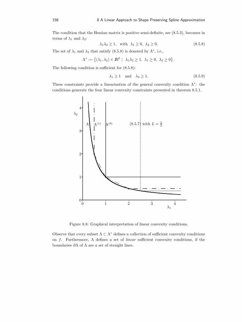
156 8 A Linear Approach to Shape Preserving Spline Approximation
The condition that the Hessian matrix is positive semi-definite, see (8.5.3), becomes interms of λ1 and λ2:
λ1λ2 ≥ 1, with λ1 ≥ 0, λ2 ≥ 0. (8.5.8)
The set of λ1 and λ2 that satisfy (8.5.8) is denoted by Λ∗, i.e.,
Λ∗ :=
(λ1, λ2) ∈ IR2 | λ1λ2 ≥ 1, λ1 ≥ 0, λ2 ≥ 0.
The following condition is sufficient for (8.5.8):
λ1 ≥ 1 and λ2 ≥ 1. (8.5.9)
These constraints provide a linearisation of the general convexity condition Λ∗: theconditions generate the four linear convexity constraints presented in theorem 8.5.1.
λ1
λ2
Λ∗ Λ(0) (8.5.7) with L = 52Λ(1)
0 1 2 3 40
1
2
3
4
rr
r
AA
AA
AA
ppHH
HHHH
p p p p p p p p
pppppp
Figure 8.8: Graphical interpretation of linear convexity conditions.
Observe that every subset Λ ⊂ Λ∗ defines a collection of sufficient convexity conditionson f . Furthermore, Λ defines a set of linear sufficient convexity conditions, if theboundaries ∂Λ of Λ are a set of straight lines.

8.5 Linear constraints for shape preservation of bivariate splines 157
We now set up a sequence Λ(k), k ∈ IN , of sets of sufficient linear convexity conditionswith the following property Λ(k) ⊂ Λ∗, ∀k. If, in addition, Λ(k) gets closer to Λ∗, theset of sufficient convexity conditions becomes weaker.These observations make it easy to set up a suitable construction for generating linearconvexity constraints. The curve λ1λ2 = 1 simply has to be divided in a number oflinear segments. This is done in the following example:
Example 8.5.4 (Weak sufficient convexity conditions) Approximate the curve λ1λ2 =1 with Nk linear segments, where Nk = 2(k+1). Define the set of knots ti as a partitionof [0, 1]: 0 = t0 < t1 < . . . < tk < 1. For example, this can be done by ti = i/(1 + k),i = 0, . . . , k. Define yi = 1− ti and xi = 1/yi, then
yi = 1− ti = 1− i
1 + k=
1 + k − i1 + k
, and xi =1yi
=1 + k
1 + k − i .
Then define the following constraints:
ci := (λ1 − xi)(yi−1 − yi) + (λ2 − yi)(xi − xi−1) ≥ 0, i = 1, . . . , k, and
di := (λ1 − yi)(xi − xi−1) + (λ2 − xi)(yi−1 − yi) ≥ 0, i = 1, . . . , k.
and
ck+1 = λ1 ≥ yk =1
1 + k= t1 and dk+1 = λ2 ≥ yk =
11 + k
= t1.
Only if t0 > 0, the additional constraint λ1 + λ2 − (x0 + y0) ≥ 0 is necessary. Thesequence Λ(k) that is constructed in this way is nested as Λ(2k) ⊂ Λ(k) and approximatesΛ∗ better as k tends to infinity. Some examples are graphically shown in figure 8.8.The case k = 0 results in the conditions (8.5.9). The conditions proposed in [CFP97]are
Lλ1 ≥ 1, Lλ2 ≥ 1, Lλ1 + λ2 ≥ L+ 1, λ1 + Lλ2 ≥ L+ 1, L ≥ 1, (8.5.10)
and L = 2 corresponds with k = 1, i.e., Λ(1) in the construction above.Furthermore, the case k = 2 results in the conditions Λ(2):
3λ1 ≥ 1, 3λ2 ≥ 1, 3λ1 + 2λ2 ≥ 5, 2λ1 + 3λ2 ≥ 5, 9λ1 + 2λ2 ≥ 9, 2λ1 + 9λ2 ≥ 9.
As before, the linear constraints on second derivatives of the function f can also beapplied to tensor-product B-splines, which generates a number of linear inequalities inthe B-spline coefficients.

158 8 A Linear Approach to Shape Preserving Spline Approximation
8.6 An iterative algorithm for shape preserving approximation
In this section, we propose an algorithm for constrained B-spline approximation. Con-sider the bivariate gridded data set (xi, yj , fi,j) ∈ IR3, but note that the restrictionto gridded data is not essential. Next, a tensor-product B-spline function u(x, y) isdefined, see (2.2.6), which is based on the knot set ξjNξj=0 in the x-direction and
ψjNψj=0 in the y-direction. These knot distributions divide the domain in Nξ × Nψsegments. The degree of the B-spline is assumed to be nx in the x-direction, and ny inthe y-direction.
The algorithm. Once some `p-norm (or `′
p-norm) is chosen, the objective function in(8.1.2) is defined. In addition, a linearisation of certain shape constraints for univariateB-splines (section 8.4) or bivariate tensor-product B-splines (section 8.5) is applied.This properly defines the approximation problem (8.1.2), which in fact results in alinear programming (LP) problem, provided p = 1,∞.Usually a solution of this constrained approximation problem does not satisfy the pre-scribed error tolerance. The common way to deal with this problem is to introduceadditional degrees of freedom. In this chapter, the dimension of the spline space isincreased by inserting additional knots (this in contrast with increasing the degree ofthe spline). Refinement of the knot vectors results in more freedom for the approxi-mant to satisfy the shape constraints as well as the required error tolerance. The ideabehind the algorithm presented here is to insert extra knots where the approximationis not good enough, and then calculating an improved approximant. The algorithmdistinguishes between ’method A’ and ’method B’; the differences between the two arediscussed later.These observations lead to the following constrained spline approximation algorithmbased on iterative knot refinement.
Algorithm 8.6.1 Given a bivariate data set (xi, yj , fi,j).
1. Define suitable initial knot sets Ξ = ξjNξj=0, and Ψ = ψjNψj=0.
2. Calculate initial constrained approximant using method A.
3. Continue loop until data are well approximated:
(a) Determine the location of the point (xi, yj) for which |u(xi, yj) − fi,j | ismaximal.
(b) Add degrees of freedom using knot insertion: If xi 6∈ Ξ, then add a knotξ1 = xi, i.e., Ξ := Ξ ∪ ξ1,

8.6 An iterative algorithm for shape preserving approximation 159
Else, add two additional knots ξ1 = (ξj−1 + xi)/2 and ξ2 = (xi + ξj+1)/2,i.e., Ξ := Ξ ∪ ξ1, ξ2.Similarly, Ψ is extended by inserting one or two knots near yj.
(c) Optional: calculate constrained spline approximant using method B. Thealgorithm is terminated if the error is smaller than the given tolerance.
(d) Calculate a new constrained spline approximant based on the extended knotsets Ξ and Ψ using method A.
The loop is terminated when the error satisfies the prescribed tolerance.
4. Optional: calculate constrained spline approximant using method B.
Next, the choice of the norm in the approximation method is discussed, i.e., whichmethod is suited for ’method A’ and ’method B’. Finally, some comments are made onknot insertion.
Remark 8.6.2 The restriction to B-splines in this algorithm is not necessary. Insteadof B-splines, one can use standard splines and add smoothness constraints, which arelinear in the spline coefficients. Another possibility is to use splines defined on a tri-angulation, and a suitable initial triangulation is the convex triangulation. Iterativetriangulation refinement is based on halving edges where the error is large. Auxiliaryfunction values, only used to determine the new convex triangulation, are assigned tothese new points using convexity preserving subdivision. ♦
Choice of the norm. We discuss which methods A and B are suitable for applicationin algorithm 8.6.1.’Method A’ has to provide appropriate locations for introducing additional knots. Asshown in the algorithm, this has to be done at locations where the error is large.Therefore `∞-approximation is not suited for the purpose of knot insertion, as it suffersfrom the alternating error behaviour of minimax-approximation, see figure 8.2.2. Least-squares approximation leads to a QP-problem, and therefore `1-approximation seems tobe the best method. The `1-method is dual to `∞, which is also clearly displayed in theerror distributions in figure 8.7. However, when rewriting `p-approximation, p = 1,∞,to an LP-problem, the number of linear constraints increases significantly in case of alarge number of data. The `
′
p methods from section 8.3 do not have this drawback.The illustrative example of approximating data from the function |x|, see figure 8.7,shows that the `
′
p-methods for p = 1 or p = ∞ are suited for the purpose of knotinsertion. The error distribution strongly suggests to add a knot at (or near) x = 0.`∞′-approximation is a little more attractive since the complexity of the LP-problem
is lower.
160 8 A Linear Approach to Shape Preserving Spline Approximation
’Method B’ is not used for knot-insertion, so any `p or `′
p approximation method withp = 1 or p = ∞ can be used for this method. It is clear that in general the maximumdifference between the spline approximation and the given data is to get smaller when`∞-approximation is used after application of any `p-norm or `
′
p-norm.
Location of the knots. The problem of choosing a suitable knot set is known to bedifficult. Some comments on this problem are made.First of all, an initial knot set has to be chosen. For unconstrained interpolation prob-lems, it is well-known that the dimension of the spline space that is necessary to inter-polate the data is at most equal to the number of data points. In the constrained casehowever, it is not simple to determine the lowest number of knots that is necessary forinterpolation. This number is generally not bounded by the number of data points, butdepends on the data set. For example for data drawn from f(x, y) = |x| on [−1, 1]2,the sketched algorithm will never be able to interpolate in a convexity preserving way.Although in many situations it will be possible to use fewer knots, a conservative andsuitable choice in general is to place a knot at every data point for the initial knot set.According to algorithm 8.6.1, one or more knots are added in every iteration. Thischoice of knot refinement has turned out to be useful in various numerical experiments,e.g., the univariate example of approximating data from f(x) = |x| which is used as anillustration in sections 8.4 and 8.5. Nevertheless, it is remarked that more effort canbe done to improve the treatment discussed in this thesis. One extension is to use thefollowing knot refinement method:
ξ1 = t ξj−1 + (1− t) xi, ξ2 = (1− t) xi + t ξi+1,
where 0 < t < 1. The choice of small values for t turned out to be more efficientin the example. The conservative and convenient choice t = 1
2 has been chosen inthe algorithm. For this value of t a homogeneous refinement near the data values isobtained. In general, an optimal value for t depends on the behaviour of the data.
For tensor-product B-splines, the insertion of new knots means that knot lines parallelto the coordinate axes have to be inserted. It is then simple to construct examples ofdifficult data for which any knot placement method requires a huge number of knots tosatisfy small error tolerances in general. To overcome this problem of tensor-productB-splines, it is more natural to apply a method based on triangulations. The convextriangulation is suitable for this purpose. Nevertheless, constrained tensor-product B-spline approximation methods are very useful for many practical applications, and notriangular method is known to work as efficient as this tensor-product B-spline methodas an approximation tool. However, methods based on triangulations could be moreefficient, see remark 8.6.2.

References
[AG93] J.C. Archer and E. Le Gruyer. Two shape preserving Lagrange c2-interpolants. Numer. Math., 64:1–11, 1993.
[But80] J. Butland. A method of interpolating reasonably-shaped curves throughany data. Proc. Computer Graphics, 80:409–422, 1980.
[C+91] B. W. Char et al. Maple V Language Reference Manual. Springer-Verlag,New York, 1991.
[Cai95] Z. Cai. Convergence, error estimation and some properties of four-pointinterpolation subdivision scheme. Comput. Aided Geom. Design, 12:459–468, 1995.
[CD94] J. M. Carnicer and W. Dahmen. Characterization of local strict convexitypreserving interpolation methods by C1 functions. J. Approx. Theory, 77:2–30, 1994.
[CDM91] A. S. Cavaretta, W. Dahmen, and C. A. Micchelli. Stationary subdivision.Memoires of the AMS, 93:1–186, 1991.
[CFP97] J. M. Carnicer, M. S. Floater, and J. M. Pena. Linear convexity conditionsfor rectangular and triangular Bernstein-Bezier surfaces. Comput. AidedGeom. Design, 15:27–38, 1997.
[Cha74] G.M. Chaikin. An algorithm for high speed curve generation. ComputerGraphics and Image Processing, 3:346–349, 1974.
[CLR80] E. Cohen, T. Lyche, and R.F. Riesenfeld. Dicrete B-splines and subdivisiontechniques in Computer Aided Geometric Design and Computer Graphics.Computer Graphics and Image Processing, 14:87–111, 1980.
[CM89] A. S. Cavaretta and C. A. Micchelli. The design of curves and surfaces bysubdivision algorithms. In T. Lyche and L. L. Schumaker, editors, Mathe-matical Methods in CAGD, pages 115–153, Boston, 1989. Academic Press.

162 References
[Cos88] P. Costantini. An algorithm for computing shape preserving interpolatingsplines of arbitrary degree. J. Comput. Appl. Math., 22:89–136, 1988.
[Cos97] P. Costantini. Variable degree polynomial splines. In A. Le Mehaute,C. Rabut, and L. L. Schumaker, editors, Curves and Surfaces with Appli-cations in CAGD, pages 85–94, Nashville, TN, 1997. Vanderbilt UniversityPress.
[Dah91] W. Dahmen. Convexity and Bernstein-Bezier polynomials. In P.-J. Laurent,A. Le Mehaute, and L. L. Schumaker, editors, Curves and Surfaces, pages107–134, Boston, 1991. Academic Press.
[dB78] C. de Boor. A Practical Guide to Splines. Springer-Verlag, New York-Heidelberg-Berlin, 1978.
[dC59] P. de Casteljau. Outilage methodes calcul. Technical report, Andre CitroenAutomobiles, SA, Paris, 1959.
[DD89] G. Deslauriers and S. Dubuc. Symmetric iterative interpolation processes.Constr. Approx., 5:49–68, 1989.
[Del89] R. Delbourgo. Shape preserving interpolation to convex data by rationalfunctions with quadratic numerator and linear denominator. IMA J. Numer.Anal., 9:123–136, 1989.
[DG83] R. Delbourgo and J.A. Gregory. C2 rational quadratic spline interpolationto monotonic data. IMA J. Numer. Anal., 3:141–152, 1983.
[DG85a] R. Delbourgo and J.A. Gregory. The determination of derivative parametersfor a monotonic rational quadratic interpolant. IMA J. Numer. Anal., 5:397–406, 1985.
[DG85b] R. Delbourgo and J.A. Gregory. Shape preserving piecewise rational inter-polation. SIAM J. Sci. Statist. Comput., 6:967–976, 1985.
[DGL87] N. Dyn, J. A. Gregory, and D. Levin. A 4-point interpolatory subdivisionscheme for curve design. Comput. Aided Geom. Design, 4:257–268, 1987.
[DGL91] N. Dyn, J. A. Gregory, and D. Levin. Analysis of uniform binary subdivisionschemes for curve design. Constr. Approx., 7(2):127–147, 1991.
[DGS97] I. Daubechies, I. Guskov, and W. Sweldens. Regularity of irregular subdivi-sion. preprint, May 1997.
References 163
[DJ87] B.E.J. Dahlberg and B. Johansson. Shape preserving approximation. InR. R. Martin, editor, The Mathematics of Surfaces II, pages 419–426, Ox-ford, 1987. Clarendon Press.
[D+98] N. Dyn, F. Kuijt, D. Levin, and R. van Damme. Convexity preservationof the four-point interpolatory subdivision scheme. Memorandum no. 1457,University of Twente, Faculty of Applied Mathematics, 1998. Submitted toComput. Aided. Geom. Design.
[DL90] N. Dyn and D. Levin. Interpolating subdivision schemes for the generationof curves and surfaces. In W. Haussmann and K. Jetter, editors, Multivari-ate Approximation and Interpolation, volume 94 of International Series ofNumerical Mathematics, pages 91–106, Basel, 1990. Birkhauser.
[DL95] N. Dyn and D. Levin. Analysis of Hermite-type subdivision schemes. InC. K. Chui and L. L. Schumaker, editors, Approximation Theory VIII, Vol.2: Wavelets and Multilevel Approximation, pages 117–124, Singapore, 1995.World Scientific.
[DL97] N. Dyn and D. Levin. Analysis of Hermite-interpolatory subdivisionschemes. In Proceedings of the workshop: Spline functions and wavelets,1997.
[DLL92] N. Dyn, D. Levin, and D. Liu. Interpolatory convexity preserving subdivisionschemes for curves and surfaces. Comput. Aided Design, 24(4):211–216, 1992.
[DM88] W. Dahmen and C.A. Micchelli. Convexity of multivariate Bernstein poly-nomials and box spline surfaces. Studia Sci. Math. Hungar., 23:265–287,1988.
[Dub86] S. Dubuc. Interpolation through an iterative scheme. J. Math. Anal. Appl.,114:185–204, 1986.
[Dyn92] N. Dyn. Subdivision schemes in Computer-Aided Geometric Design. InW. Light, editor, Wavelets, Subdivision Algorithms, and Radial Basis Func-tions, volume II of Advances in Numerical Analysis, pages 36–104, Oxford,1992. Clarendon Press.
[Far90] G.E. Farin. Curves and Surfaces for Computer Aided Geometric Design - Apractical guide. Academic Press, San Diego, second edition, 1990.
[FB84] F. N. Fritsch and J. Butland. A method for constructing local monotonepiecewise cubic interpolants. SIAM J. Sci. Statist. Comput., 5:300–304,1984.

164 References
[FM98] M. S. Floater and C. A. Micchelli. Nonlinear stationary subdivision. InApproximation Theory, volume 212 of Monogr. Textbooks Pure Appl. Math.,pages 209–224, New York, 1998. Dekker.
[GD82] J. A. Gregory and R. Delbourgo. Piecewise rational quadratic interpolationto monotonic data. IMA J. Numer. Anal., 2:123–130, 1982.
[GQ96] J. A. Gregory and R. Qu. Nonuniform corner cutting. Comput. Aided Geom.Design, 13:763–772, 1996.
[HJ98] B. Han and R.-Q. Jia. Multivariate refinement equations and convergenceof subdivision schemes. SIAM J. Math. Anal., 29:1177–1199, 1998.
[Iqb92] R. Iqbal. A one-pass algorithm for shape-preserving quadratic spline inter-polation. J. Sci. Comput., 7:359–376, 1992.
[JRZ98] R.-Q. Jia, S.D. Riemenschneider, and D.-X. Zhou. Vector subdivisionschemes and multiple wavelets. Math. Comp., 67:1533–1563, 1998.
[Jut97a] B. Juttler. Arbitrarily weak linear convexity conditions for multivariatepolynomials. Technical report, University of Technology, Department ofMathematics, Darmstadt, Germany, 1997.
[Jut97b] B. Juttler. Surface fitting using convex tensor-product splines. J. Comput.Appl. Math., 84:23–44, 1997.
[KvD97a] F. Kuijt and R. van Damme. Monotonicity preserving interpolatory sub-division schemes. Memorandum no. 1402, University of Twente, Faculty ofApplied Mathematics, 1997. Submitted to J. Comput. Appl. Math.
[KvD97b] F. Kuijt and R. van Damme. Shape preserving interpolatory subdivisionschemes for nonuniform data. Memorandum no. 1423, University of Twente,Faculty of Applied Mathematics, 1997. Submitted to J. Approx. Theory.
[KvD97c] F. Kuijt and R. van Damme. Smooth interpolation by a convexity preservingnonlinear subdivision algorithm. In A. Le Mehaute, C. Rabut, and L. L.Schumaker, editors, Surface Fitting and Multiresolution Methods, pages 219–224, Nashville, TN, 1997. Vanderbilt University Press.
[KvD98a] F. Kuijt and R. van Damme. Convexity preserving interpolatory subdivisionschemes. Constr. Approx., 14(4):609–630, 1998.
[KvD98b] F. Kuijt and R. van Damme. Hermite-interpolatory subdivision schemes.Memorandum no. 1461, University of Twente, Faculty of Applied Mathe-matics, 1998. Submitted to SIAM J. Math. Anal.
References 165
[KvD98c] F. Kuijt and R. van Damme. A linear approach to shape preserving splineapproximation. Memorandum no. 1450, University of Twente, Faculty ofApplied Mathematics, 1998. Submitted to Adv. Comput. Math.
[KvD98d] F. Kuijt and R. van Damme. Shape preserving C2 interpolatory subdivisionschemes. Memorandum no. 1452, University of Twente, Faculty of AppliedMathematics, 1998. Submitted to Numer. Algorithms.
[Lev98] D. Levin. Using Laurent polynomial representation for the analysis of non-uniform binary subdivision schemes. Technical report, Tel-Aviv University,1998.
[LR80] J.M. Lane and R.F. Riesenfeld. A theoretical development for the computergeneration of piecewise polynomial surfaces. IEEE Trans. on Pattern Anal.and Machine Intelligence, 2:35–46, 1980.
[LU94] A. LeMehaute and F.I. Utreras. Convexity-preserving interpolatory subdi-vision. Comput. Aided Geom. Design, 11:17–37, 1994.
[Mer92] J.-L. Merrien. A family of Hermite interpolants by bisection algorithms.Numer. Algorithms, 2:187–200, 1992.
[Mer94] J.-L. Merrien. Dyadic Hermite interpolation on a triangulation. In J.C.Mason and M.G. Cox, editors, Numerical Algorithms 7, pages 391–410.J.C.Baltzer AG, 1994.
[Mic95] C.A. Micchelli. Mathematical Aspects of Geometric Modeling. SIAM,Philadelphia, PA, 1995.
[MS97] C.A. Micchelli and T. Sauer. Regularity of multiwavelets. Adv. Comput.Math., 7:455–545, 1997.
[Rie75] R.F. Riesenfeld. On Chaikin’s algorithm. Computer Graphics and ImageProcessing, 4:304–310, 1975.
[Sch73] R. Schaback. Spezielle rationale Splinefunktionen. J. Approx. Theory, 7:281–292, 1973.
[Sch82] L.L. Schumaker. Spline Functions, Basic Theory. John Wiley, 1982.
[Sch83] L. L. Schumaker. On shape preserving quadratic spline interpolation. SIAMJ. Numer. Anal., 20:854–864, 1983.

166 References
[vD91] R. van Damme. A C2 interpolating subdivision scheme for curves. Mem-orandum no. 986, University of Twente, Faculty of Applied Mathematics,1991.
[vD97] R. van Damme. Bivariate Hermite subdivision. Comput. Aided Geom. De-sign, 14:847–875, 1997.
[War95] J. Warren. Binary subdivision schemes for functions over irregular knotsequences. In M. Dæhlen, T. Lyche, and L. L. Schumaker, editors, Math-ematical Methods for Curves and Surfaces, pages 543–562, Nashville TN,1995. Vanderbilt University Press.
[YDL98] T.P.Y. Yu, N. Dyn, and D. Levin. Optimal regularity bounds for Hermite-interpolatory subdivision schemes. Preprint, Department of Statistics, Stan-ford University, 1998.
[YS93] I. Yad-Shalom. Monotonicity preserving subdivision schemes. J. Approx.Theory, 74:41–58, 1993.

Summary
This thesis deals with interpolation and approximation while preserving shape condi-tions. The problem is defined as follows. Given is a set of points, the data, whichpossesses certain shape properties, such as convexity or monotonicity. The questionis to construct a function, for example a curve or a surface, that describes these datawell and that possesses the same shape properties. A function describes the given datawell when it interpolates the data or, otherwise, when it approximates the data well ina suitable norm. The additional requirement on the function is that it is sufficientlysmooth, i.e., it is at least continuously differentiable.The techniques described in this thesis can be split up into two groups. The first, moretraditional group deals with the use of splines, which consist of piecewise polynomials.The requirement on the shape is attained by imposing conditions on the coefficientsof these splines. The conditions are most convenient if they are linear in the splinecoefficients. Therefore, attention is paid to the linearisation of conditions for convexityand monotonicity. Beside the examination of linear conditions several linear objectivefunctions are investigated and compared.The second group of methods are so-called subdivision schemes, of which the linearfour-point scheme is a well-known example. In subdivision, new points are insertedbetween existing data points by calculation from a local group of data points. Thedensity of the data can be increased to arbitrarily high level by repeated application ofthis process. In the limit of infinitely many data points a function which interpolatesthe given data is obtained, and, in addition, this function is continuous or even oneor more times continuously differentiable. For most applications however, a limitednumber of iterations is sufficient to arrive at a useful result. As, in addition, subdivisionmethods are local, above mentioned iteration process requires a relatively small amountof computational effort.In this thesis, special attention is paid to shape preserving subdivision, with an empha-sis on methods that preserve convexity. In addition, methods that preserve monotonic-ity or positivity are examined. First, convexity preserving subdivision for univariateequidistant data is investigated. A four-point interpolatory rational scheme that pre-

168 Summary
serves convexity is constructed. If the original data are strictly convex, this algorithmconverges to convex C1 limit functions. Using a similar approach, a class of four-pointrational subdivision methods that preserve monotonicity and that also generate C1
limit functions is constructed. These schemes all have approximation order four.With respect to subdivision for non-equidistant data, the parameter values have to besubdivided by a subdivision method that preserves monotonicity, which keeps the gridordered. Using a suitable monotonicity preserving scheme a grid is created that becomesincreasingly locally uniform. With this knowledge, convexity preserving subdivision canbe generalised to nonequidistant data. A subdivision algorithm of third order whichleads to convex C1 limit functions for any strictly convex data is constructed.A relation between methods for shape preserving rational spline interpolation andsubdivision exists. Based on e.g., convexity preserving rational splines, a subdivisionscheme that preserves convexity can be constructed. However, this is not an exhaust-ing method for convexity preserving subdivision, because subdivision can be seen as ageneralisation of splines. Using a generalisation of C1 rational splines, subdivision algo-rithms are constructed that also preserve convexity or monotonicity, but these schemesare more smooth. This leads to for example six-point rational subdivision algorithmsthat generate C2 limit functions and that preserve convexity. The smoothness of thelimit function of these six-point schemes is hard to determine analytically. However, asimple numerical method for validation of the smoothness of subdivision methods canbe formulated.To interpolate function values as well as derivatives, Hermite-interpolatory subdivisionschemes are examined. A class of linear C2 Hermite schemes is constructed. In addi-tion, simple rational Hermite schemes which preserve convexity and generate smoothfunctions are presented.

Samenvatting
Het thema van dit proefschrift is interpolatie en approximatie onder vormbehoudendevoorwaarden. Het probleem is als volgt gedefinieerd. Gegeven is een verzamelingpunten, de data, die bepaalde eigenschappen bezitten aangaande hun onderlinge ligging,zoals convexiteit of monotoniciteit. Gevraagd is een functie te bepalen, bijvoorbeeld eenkromme of een oppervlak, die deze data goed beschrijft en dezelfde vorm-eigenschappenbezit. Een functie beschrijft de gegeven data goed als deze door de data gaat, d.w.zinterpolatie, of anders in een geschikte norm dicht bij de data ligt, d.w.z. approximatie.De aanvullende eis op deze benaderende functie is dat deze voldoende glad is, nl.tenminste een maal continu differentieerbaar.De beschreven technieken in dit proefschrift laten zich ruwweg verdelen in twee groepen.De eerste, meer traditionele groep betreft het gebruik van splines die bestaan uit stuks-gewijze polynomen. De vereiste vorm wordt bereikt door het opleggen van voorwaardenop de coefficienten van deze splines. De nadruk ligt op voorwaarden die lineair zijn inde spline-coefficienten en de gewenste vorm garanderen. Er wordt daarom aandachtbesteed aan het lineariseren van de voorwaarden voor convexiteit en monotoniciteit.Naast het bestuderen van lineaire voorwaarden worden ook verschillende lineaire doel-functies onderzocht en vergeleken.De tweede groep van methoden die in dit proefschrift onderzocht worden, zijn zoge-naamde subdivisieschema’s, waarvan het lineaire vier-punts schema een bekend voor-beeld is. Bij subdivisie worden tussen bestaande datapunten nieuwe punten toegevoegddoor berekening vanuit een beperkte groep van nabije datapunten. Door dit procesvoortdurend te herhalen kan de puntendichtheid willekeurig opgevoerd worden, en inde limiet van oneindig veel punten is een functie ontstaan die de oorspronkelijke pun-ten interpoleert, en die bovendien continu is of zelfs een of meerdere malen continudifferentieerbaar. Voor de meeste toepassingen is daarentegen een beperkt aantal ite-raties toereikend om tot een voldoende resultaat te komen. Omdat subdivisiemethodenbovendien lokaal zijn vereist bovenstaand iteratieproces relatief weinig rekenkracht.In dit proefschrift wordt vooral aandacht geschonken aan vormbehoudende subdivisie,waarbij de nadruk ligt op methoden die convexiteit behouden. Daarnaast zijn metho-

170 Samenvatting
den onderzocht die monotoniciteit of positiviteit behouden. Allereerst wordt convexi-teitsbehoudende subdivisie voor univariate equidistante data bestudeerd. Een vier-punts interpolerend rationaal schema dat convexiteit behoudt wordt geconstrueerd.Als de oorspronkelijke data een strikt convexe ligging vertonen, convergeert dit algo-ritme naar C1 limietfuncties die eveneens convex zijn. Met een soortgelijke aanpakwordt een klasse van vier-punts rationale subdivisiemethoden geconstrueerd die mono-toniciteit behouden en eveneens C1 limietfuncties genereren. Deze schema’s hebbenalle approximatie-orde vier.Met betrekking tot subdivisie voor niet-equidistante data dient voor de parameter-waarden een subdivisiemethode gebruikt te worden die monotoniciteit behoudt, waar-mee het grid geordend blijft. Met een geschikt monotoniciteitsbehoudend schemaontstaat een grid dat meer en meer lokaal uniform wordt. Hiermee wordt convexi-teitsbehoudende subdivisie gegeneraliseerd tot niet-equidistante data. Een subdivisie-algoritme van de derde orde is geconstrueerd dat leidt tot convexe C1 limietfuncties bijstrikt convexe data.Er wordt een relatie gelegd met methoden voor vormbehoudende rationale spline-interpolatie. Op basis van bijvoorbeeld convexiteitsbehoudende rationale splines kaneen subdivisieschema worden geconstrueerd dat convexiteit behoudt. Dit is echtergeen uitputtende methode voor convexiteitsbehoudende subdivisie, omdat subdivisie tebeschouwen is als een generalisatie van splines. Door gebruik te maken van een generali-satie van C1 rationale splines kunnen subdivisie-algoritmen worden geconstrueerd dieeveneens convexiteit of monotoniciteit behouden maar gladder zijn. Dit leidt bijvoor-beeld tot zes-punts rationale subdivisie-algoritmen die C2 limietfuncties genereren enconvexiteit behouden. De gladheid van de limietfunctie van deze zes-punts schema’sis echter moeilijk analytisch te bepalen. Een eenvoudige numerieke methode voor devalidatie van de gladheid van subdivisie-methoden kan wel worden geformuleerd.Om naast functiewaarden ook afgeleiden te interpoleren, zijn Hermite-interpolerendesubdivisieschema’s bestudeerd. In dit verband wordt een klasse van C2 lineaire Her-mite schema’s geconstrueerd. Eveneens worden eenvoudige rationale Hermite schema’sgepresenteerd die convexiteit behouden en gladde functies genereren.

Dankwoord
Dit proefschrift is tot stand gekomen na een periode van vier jaar onderzoek aan deUniversiteit Twente te Enschede. Velen hebben direct of indirect een bijdrage geleverdaan het verkregen resultaat.Allereerst bedank ik mijn promotor Cees Traas voor zijn algemene supervisie. Dezekenmerkte zich door een ruime mate van vrijheid gecombineerd met gerichte sturingwaar dat nodig was. Zijn precieze wijze van formuleren heeft daarnaast bijgedragentot de leesbaarheid van de definitieve versie van dit proefschrift.Vooral door intensieve samenwerking en vele stimulerende discussies met mijn dagelijksebegeleider Ruud van Damme is dit proefschrift in de huidige vorm gekomen. Regelmatigvormde Ruud voor mij het levende bewijs dat een praktische en pragmatische instellingook leidt tot theoretische resultaten en diepgaand inzicht. Zijn precisie noodzaakte mijmeer dan eens tot verder nadenken.Niet alleen de uitstekende organisatie bij de technologiestichting STW, maar ook deenthousiaste inbreng van de diverse leden van de gebruikerscommissie komend uit hetbedrijfsleven, heb ik bijzonder gewaardeerd. Ik kijk eveneens met genoegen terug opde periodieke bijeenkomsten van de landelijke werkgroep Spline Approximatie.Tijdens en na conferentiebezoek heb ik nuttige suggesties gekregen van Nira Dyn. Ditleidde tot een bijzonder interessant werkbezoek aan Israel, waar ik prettig met haar enDavid Levin van de Universiteit van Tel-Aviv heb samengewerkt.Verder hebben mijn collega’s van de afdeling bijgedragen aan een goede werksfeer. Hier-bij denk ik onder andere aan mijn kamergenoot Matthijs Toose. Daarnaast hebben ver-schillende collega’s geholpen bij wiskundige vragen en computertechnische problemen.De gezellige koffiepauzes zal ik niet snel vergeten.Tenslotte ben ik mijn ouders, familie en vrienden dankbaar voor hun belangstelling enbetrokkenheid door de jaren heen. Vooral denk ik aan de onmisbare aandacht, liefdeen geduld die ik van mijn vrouw Eveline, en sinds kort ook van onze zoon Gideon,gekregen heb.
Enschede, september 1998.