
Observable set, observability, interpolation inequality and ...
44
Observable set, observability, interpolation inequality and spectral inequality for the heat equation in R n Gengsheng Wang * Ming Wang † Can Zhang ‡ Yubiao Zhang § November 12, 2017 Abstract This paper studies connections among observable sets, the observability inequality, the H¨ older-type interpolation inequality and the spectral inequality for the heat equation in R n . We present a characteristic of observable sets for the heat equation. In more detail, we show that a measurable set in R n satisfies the observability inequality if and only if it is γ-thick at scale L for some γ> 0 and L> 0. We also build up the equivalence among the above-mentioned three inequalities. More precisely, we obtain that if a measurable set E ⊂ R n satisfies one of these inequalities, then it satisfies others. Finally, we get some weak observability inequalities and weak interpolation inequalities where observations are made over a ball. Keywords: Characteristic of observable sets, observability inequality, H¨ older-type interpola- tion inequality, spectral inequality, heat equation AMS subject classifications: 49J20, 49K20, 93D20 Contents 1 Introduction 2 1.1 Thick sets and several inequalities ........................... 2 1.2 Aim, motivation and main result ............................ 6 1.3 Extensions to bounded observable sets ......................... 8 1.4 Plan of the paper ..................................... 9 2 Proof of Theorem 1.1 9 3 Weak interpolation and observability inequalities 22 3.1 Weak interpolation inequalities with observation on the unit ball .......... 22 3.2 Weak observability inequalities with observations on balls .............. 35 * School of Mathematics and Statistics, Wuhan University, Wuhan, 430072, China. Email: [email protected] † School of Mathematics and Physics, China University of Geosciences, Wuhan, 430074, China. Email: [email protected] ‡ School of Mathematics and Statistics, Wuhan University, Wuhan, 430072, China, and Department of Mathe- matics, University of the Basque Country (UPV/EHU), Bilbao, 48080, Spain. Email: [email protected] § Center for Applied Mathematics, Tianjin University, Tianjin, 300072, China. Email: [email protected] 1
-
Upload
khangminh22 -
Category
Documents
-
view
1 -
download
0
Transcript of Observable set, observability, interpolation inequality and ...

Observable set, observability, interpolation
inequality and spectral inequality for the heat
equation in Rn
Gengsheng Wang∗ Ming Wang† Can Zhang‡ Yubiao Zhang§
November 12, 2017
Abstract
This paper studies connections among observable sets, the observability inequality, theHolder-type interpolation inequality and the spectral inequality for the heat equation in Rn.We present a characteristic of observable sets for the heat equation. In more detail, weshow that a measurable set in Rn satisfies the observability inequality if and only if it isγ-thick at scale L for some γ > 0 and L > 0. We also build up the equivalence amongthe above-mentioned three inequalities. More precisely, we obtain that if a measurable setE ⊂ Rn satisfies one of these inequalities, then it satisfies others. Finally, we get some weakobservability inequalities and weak interpolation inequalities where observations are made overa ball.
Keywords: Characteristic of observable sets, observability inequality, Holder-type interpola-tion inequality, spectral inequality, heat equation
AMS subject classifications: 49J20, 49K20, 93D20
Contents
1 Introduction 21.1 Thick sets and several inequalities . . . . . . . . . . . . . . . . . . . . . . . . . . . 21.2 Aim, motivation and main result . . . . . . . . . . . . . . . . . . . . . . . . . . . . 61.3 Extensions to bounded observable sets . . . . . . . . . . . . . . . . . . . . . . . . . 81.4 Plan of the paper . . . . . . . . . . . . . . . . . . . . . . . . . . . . . . . . . . . . . 9
2 Proof of Theorem 1.1 9
3 Weak interpolation and observability inequalities 223.1 Weak interpolation inequalities with observation on the unit ball . . . . . . . . . . 223.2 Weak observability inequalities with observations on balls . . . . . . . . . . . . . . 35
∗School of Mathematics and Statistics, Wuhan University, Wuhan, 430072, China. Email: [email protected]†School of Mathematics and Physics, China University of Geosciences, Wuhan, 430074, China. Email:
[email protected]‡School of Mathematics and Statistics, Wuhan University, Wuhan, 430072, China, and Department of Mathe-
matics, University of the Basque Country (UPV/EHU), Bilbao, 48080, Spain. Email: [email protected]§Center for Applied Mathematics, Tianjin University, Tianjin, 300072, China. Email: [email protected]
1

1 Introduction
In this paper, we consider the heat equation in the whole physical space Rn:
∂tu−4u = 0 in (0,∞)× Rn, u(0, ·) ∈ L2(Rn). (1.1)
For this equation, we will characterize the observable sets and build up connections among severalimportant inequalities which are introduced in the next subsection.
Notation Write C(· · · ) for a positive constant that depends on what are included in the bracketsand may vary in different contexts. The same can be said about C ′(· · · ), C1(· · · ) and so on. UseVn to denote the volume of the unit ball in Rn. Let Br(x), with x ∈ Rn and r > 0, be the ballin Rn, centered at x and of radius r. (Simply write Br = Br(0).) Let Sn−1 be the unit sphericalsurface in Rn. Denote by Q the open unit cube in Rn, centered at the origin. Let x + LQ, withx ∈ Rn and L > 0, be the set x + Ly : y ∈ Q. For each measurable D ⊂ Rn, denote by |D|its Lebesgue measure. Given f ∈ L2(Rn), write f for its Fourier transform1. Let et4 : t ≥ 0be the semigroup generated by the Laplacian operator in Rn. Given x = (x1, . . . , xn) ∈ Rn, let
|x| :=(∑n
i=1 x2i
)1/2and 〈x〉 :=
√1 + |x|2.
1.1 Thick sets and several inequalities
We start with introducing sets of γ-thick at scale L.
Sets of γ-thick at scale L A measurable set E ⊂ Rn is said to be γ-thick at scale L for someγ > 0 and L > 0, if ∣∣∣E⋂(x+ LQ)
∣∣∣ ≥ γLn for each x ∈ Rn. (1.2)
About sets of γ-thick at scale L, several remarks are given in order.
(a1) To our best knowledge, this definition arose from studies of the uncertainty principle. Wequote it from [5] (see Page 5 in [5]). Before [5], some very similar concepts were proposed.For instance, the definition of relative dense sets was given in [23] (see also Page 113 in [19]);the definition of thick sets was introduced in [24].
(a2) Each set E of γ-thick at scale L has the following properties: First, in each cube with thelength L, |E| is bigger than or equals to γLn. Consequently, E has a positive Lebesguemeasure in each neighborhood of every x in Rn. Second, E is also a set of γ-thick at scale2L, but the reverse is not true. Third, we necessary have that γ ≤ 1.
Next, we introduce an observability inequality for the equation (1.1).
The observability inequality A measurable set E ⊂ Rn is said to satisfy the observability in-equality for the equation (1.1), if for any T > 0 there exists a positive constant Cobs = Cobs(n, T,E)so that when u solves (1.1),∫
Rn|u(T, x)|2 dx ≤ Cobs
∫ T
0
∫E
|u(t, x)|2 dxdt. (1.3)
1 Given f in the Schwartz class S(Rn), its Fourier transform is as: f(ξ) = (2π)−n∫Rn e
−ixξf(x) dx, ξ ∈ Rn.
Since S(Rn) is dense in L2(Rn), by a standard way, we can define f for each f ∈ L2(Rn).
2

When a measurable E ⊂ Rn satisfies (1.3), it is called an observable set for (1.1).Several notes on the observability inequality (1.3) are given in order.
(b1) Being treated the integral on the left hand side as a recovering term, and the integral on theright hand side as an observation term, the inequality (1.3) can be understood as: one canrecover a solution of (1.1) at time T , via observing it on the set E and in the time interval(0, T ). From perspective of control theory, the inequality (1.3) is equivalent to the followingnull controllability: For any u0 ∈ L2(Rn) and T > 0, there exists a control f ∈ L2((0, T )×Rn)driving the solution u to the controlled equation: ∂tu −4u = χEf in (0, T ) × Rn, from theinitial state u0 to the state 0 at time T . (Here, χE is the characteristic function of E.)
(b2) We can compare (1.3) with the observability inequality for the heat equation on a boundedphysical domain. Let Ω be a bounded C2 (or Lipschitz and locally star-shaped, see [2])domain in Rn. Consider the equation:
∂tu−4u = 0 in (0,∞)× Ω,
u = 0 on (0,∞)× ∂Ω,
u(0, ·) ∈ L2(Ω).
(1.4)
We say a measurable set ω ⊂ Ω satisfies the observability inequality for (1.4), if given T > 0,there is a constant C(n, T, ω,Ω) > 0 so that when u solves (1.4),∫
Ω
|u(T, x)|2 dx ≤ C(n, T, ω,Ω)
∫ T
0
∫ω
|u(t, x)|2 dx dt. (1.5)
When a measurable set ω ⊂ Ω satisfies (1.5), it is called an observable set for (1.4).
The inequality (1.5) has been widely studied. See [18, 27, 32] for the case where ω is open;[1, 2, 16] for the case when ω is measurable.
(b3) When Ω is an unbounded domain and ω is bounded and open subset of Ω, the inequality (1.5)may not be true. This was showed in [35] for the heat equation in the physical domain R+.Similar results have been obtained for higher dimension cases in [36]. For the heat equationin an unbounded domain, [37] imposed a condition, in terms of the Gaussian kernel, on theset ω so that the observability inequality does not hold. In particular, [37] showed thatthe observability inequality fails when |ω| < ∞. Notice that for the heat equation (1.1),any set E of finite measure does not have the characteristic on observable sets of (1.1).This characteristic is indeed the γ-thickness at scale L for some γ > 0 and L > 0. (SeeTheorem 1.1 of this paper.)
About works on sufficient conditions of observable sets for heat equations in unboundeddomains, we would like to mention the work [7]. It showed that, for some parabolic equationsin an unbounded domain Ω ⊂ Rn, the observability inequality holds when the observationis made over a subset E ⊂ Ω, with Ω\E bounded. For other similar results, we refer thereader to [38]. When Ω = Rn, such a set E has the characteristic on observable sets of (1.1)mentioned before.
(b4) An interesting phenomenon is that some potentials (growing at infinity) in heat equationsmay change the above-mentioned characteristic on observable sets for the heat equationswith potentials. In [39, 9], the authors realized the following fact: Let A = 4 + V , whereV (x) := −|x|2k, x ∈ Rn, with 2 ≤ k ∈ N. Write
etAt≥0
for the semigroup generated by
3

the operator A. Let r0 ≥ 0 and let Θ0 be an open subset of Sn−1. Let Γ = x ∈ Rn : |x| ≥r0, x/|x| ∈ Θ0. Then there is C(n, T,Θ0, r0, k) > 0 so that∫
Rn
∣∣eTAu0
∣∣2 dx ≤ C(n, T,Θ0, r0, k)
∫ T
0
∫Γ
∣∣etAu0
∣∣2 dxdt for all u0 ∈ L2(Rn). (1.6)
The cone Γ does not have the characteristic on observable sets mentioned before, but stillholds the observability inequality (1.6). The main reason is that the unbounded potentialV plays an important role in the proof of (1.6) (see [39, 9]). It should be pointed out thatwhen V (x) = −|x|, x ∈ Rn (which means that the potential grows more slowly at infinity),(1.6) does not hold for the above cone. We refer the readers to [39, 9] for more details onthis issue. Besides, we also would like to mention [3] for this subject.
An interesting question now arises: How do potentials influence characteristics of observablesets? We wish to answer this question in our future studies.
We then introduce an interpolation inequality for the equation (1.1).
The Holder-type interpolation inequality A measurable set E ⊂ Rn is said to satisfy theHolder-type interpolation inequality for the heat equation (1.1), if for any θ ∈ (0, 1), there isCHold = CHold(n,E, θ) > 0 so that for each T > 0 and each solution u to the equation (1.1),∫
Rn|u(T, x)|2 dx ≤ eCHold(1+ 1
T )(∫
E
|u(T, x)|2 dx)θ(∫
Rn|u(0, x)|2 dx
)1−θ. (1.7)
Several remarks on the Holder-type interpolation inequality (1.7) are given in order.
(c1) The inequality (1.7) is a kind of quantitative unique continuation for the heat equation (1.1).It provides a Holder-type propagation of smallness for solutions of the heat equation (1.1).
In fact, if
∫E
|u(T, x)|2 dx = δ, then we derive from (1.7) that
∫Rn|u(T, x)|2 dx is bounded
by Cδθ for some constant C > 0. Letting δ → 0, we find that u(T, x) = 0 for almost everyx ∈ Rn.
(c2) From perspective of control theory, the inequality (1.7) implies the approximate null control-lability with cost for impulse controlled heat equations, i.e., for any T > τ > 0, ε > 0 andany u0 ∈ L2(Rn), there is f ∈ L2(Rn) and C = C(n,E, T, τ, ε) > 0 so that
‖f‖L2(Rn) ≤ C‖u0‖L2(Rn) and ‖u(T, ·)‖L2(Rn) ≤ ε‖u0‖L2(Rn),
where u is the solution to the impulse controlled equation: ∂tu−∆u = δt=τχEf in (0, T )×Rn, with the initial condition u(0, x) = u0(x), x ∈ Rn. (See [45, Theorem 3.1].)
(c3) The Holder-type interpolation inequality (1.7) can imply the observability inequality (1.3).Moreover, it leads to the following stronger version of (1.3):∫
Rn|u(T, x)|2 dx ≤ Cobs
∫F
∫E
|u(t, x)|2 dxdt, with Cobs = Cobs(n, T,E, F ), (1.8)
where F ⊂ (0, T ) is a subset of positive measure. This will be presented in Lemma 2.4. Ourmethods used to prove (1.8) are very similar to those developed in [44, 46, 2] where heatequations on bounded domains are considered.
4

(c4) We can compare (1.7) with an interpolation inequality for heat equation (1.4). A measurableset ω ⊂ Ω is said to satisfy the Holder-type interpolation inequality for the equation (1.4), iffor any θ ∈ (0, 1) and T > 0, there is C = C(n, T,Ω, ω, θ) so that when u solves (1.4),∫
Ω
|u(T, x)|2 dx ≤ C(∫
ω
|u(T, x)|2 dx)θ(∫
Ω
|u(0, x)|2 dx)1−θ
. (1.9)
In [43], the authors proved that any open and nonempty subset ω ⊂ Ω satisfies the Holder-type interpolation inequality (1.9) for heat equations with potentials in bounded and convexdomains. The frequency function method used in [43] were partially borrowed from [11].In [2], the authors proved that any subset ω of positive measure satisfies the Holder-typeinterpolation inequality (1.9) for the heat equation (1.4) where Ω is a bounded Lipschitz andlocally star-shaped domain in Rn. More about this inequality for heat equations in boundeddomains, we referee the readers to [44, 45, 46].
Finally, we will introduce a spectral inequality for some functions in L2(Rn).
The spectral inequality A measurable set E ⊂ Rn is said to satisfy the spectral inequality, ifthere is a positive constant Cspec = Cspec(n,E) so that for each N > 0,∫
Rn|f(x)|2 dx ≤ eCspec(1+N)
∫E
|f(x)|2 dx for all f ∈ L2(Rn) with suppf ⊂ BN . (1.10)
Several notes on the spectral inequality (1.10) are given in order.
(d1) Recall the Lebeau-Robbiano spectral inequality (see [27, 28]): Let Ω be a bounded smoothdomain in Rn and let ω be a nonempty open subset of Ω. Write 4Ω for the Laplacianoperator on L2(Ω) with Domain(4Ω) = H1
0 (Ω)⋂H2(Ω). Let λjj≥1 (with λ1 < λ2 ≤ · · · )
be the eigenvalues of −4Ω and let φjj≥1 be the corresponding eigenfunctions. Then thereis a positive constant C(Ω, ω) so that∫
Ω
|f(x)|2 dx ≤ eC(Ω,ω)(1+√λ)
∫ω
|f(x)|2 dx for all f ∈ spanφj ;λj ≤ λ. (1.11)
This inequality was extended to the case where Ω is a bounded C2 domain via a simplerway in [33]. Then it was extended to the case that Ω is a bounded Lipschitz and locallystar-shaped domain, ω is a subset of positive measure and C(Ω, ω) = C(Ω, |ω|) (see Theorem5 in [2]).
By our understanding, the inequality (1.10) is comparable to (1.11) from two perspectives asfollows: First, the inequality (1.10) is made for the subspace:
EN , g ∈ L2(Rn) : suppg ⊂ BN with N > 0,
while the inequality (1.11) is made for the subspace:
Fλ , ∑λj≤λ
ajej ∈ L2(Ω) : ajj≥1 ⊂ R with λ > 0.
From the definition of the spectral projection in the abstract setting given in [48] (see Pages262-263 in [48]), we can define two spectral projections: χ[0,N2](−∆) and χ[0,λ](−∆Ω) onL2(Rn) and L2(Ω), respectively. Then after some computations, we find that EN and Fλare the ranges of χ[0,N2](−∆) and χ[0,λ](−∆Ω), respectively. Second, the square root of theintegral of χ[0,N2] over R is N which corresponds to the N in (1.10), while the square root
of the integral of χ[0,λ] over R is√λ which corresponds to the
√λ in (1.11).
5

(d2) Though the inequality (1.10) was first named as the spectral inequality in [30] (to our bestknowledge), it has been studied for long time. (See, for instance, [5, 19, 23, 24, 40, 31, 41,42, 49].) In [24], the author announced that if E is γ-thick at scale L for some γ > 0 andL > 0, then E satisfies the spectral inequality (1.10), and further proved this announcementfor the case when n=1. Earlier, the authors of [31] proved that E is γ-thick at scale L forsome γ > 0 and L > 0 if and only if E satisfies the following inequality: For each N > 0,there is a positive constant C(n,E,N) so that∫
Rn|f(x)|2 dx ≤ C(n,E,N)
∫E
|f(x)|2 dx for each f ∈ L2(Rn) with suppf ⊂ BN . (1.12)
This result is often referred as the Logvinenko-Sereda theorem. Before [31], the above equiv-alence was proved by B. P. Paneyah for the case that n = 1 (see [42, 41, 19]).
The constant C(n,E,N) in (1.12) was not expressed explicitly in terms of N in [31]. Fromthis point of view, (1.12) is weaker than the spectral inequality (1.10). In the proof of ourmain theorem of this paper, the expression C(n,E,N) = eCspec(1+N) will play an importantrole.
(d3) The inequality (1.12) is also important. It is closely related to the uncertainty principle(which is an extensive research topic in the theory of harmonic analysis and says roughlythat a nonzero function and its Fourier transform cannot be both sharply localized, see [17]).In fact, a set E of γ-thick at scale L satisfies the inequality (1.12) if and only if it satisfiesthe following uncertainty principle:∫
Rn|f(x)|2 dx ≤ C ′(n,E,N)
(∫E
|f(x)|2 dx+
∫BcN
|f(ξ)|2 dξ
)for all f ∈ L2(Rn),
where C ′(n,E,N) > 0 and BcN is the complement set of BN in Rn. We refer the interestedreaders to [5, 19, 40] for the proof of the above result, as well as more general uncertaintyprinciple, where E and BcN are replaced by more general sets.
It deserves mentioning what follows: The uncertainty principle can help us to get the exactcontrollability for the Schrodinger equation with controls located outside of two balls and attwo time points. This was realized in [52]. (See [25] for more general cases.)
(d4) By using a global Carleman estimate, the authors in [30] proved the spectral inequality (1.10)for such an open subset E that satisfies the property: there exists δ > 0 and r > 0 so that
∀y ∈ Rn,∃ y′ ∈ E such that Br(y′) ⊂ E and |y − y′| ≤ δ. (1.13)
It is clear that a set with the above property (1.13) is a set of γ-thick at scale L for someγ > 0 and L > 02.
1.2 Aim, motivation and main result
Aim According to the note (d2) in the previous subsection, the characteristic of a measurable setholding the spectral inequality (1.10) is the γ-thickness at scale L for some γ > 0 and L > 0.Natural and interesting questions are as follows: What is the characteristic of observable sets for(1.1)? How to characterize a measurable set E satisfying the Holder-type interpolation inequality(1.7)? What are the connections among inequalities (1.3), (1.7) and (1.10)? The aim of this paperis to answer the above questions.
Motivation The motivations of our studies are given in order.
2In fact, one can choose L = 2(δ + r), γ = rn (2(δ + r))−n Vn.
6

(i) The first motivation arises from two papers [4] and [1]. In [4], the authors gave, for thewave equation in a bounded physical domain Ω ⊂ Rn, a sufficient and almost necessarycondition to ensure an open subset Γ ⊂ ∂Ω to be observable, (i.e., Γ satisfies the observabilityinequality for the wave equation with observations on Γ). This condition is exactly the wellknown Geometric Control Condition (GCC for short)3. Thus, we can say that the GCCcondition is a characteristic of observable open sets on ∂Ω, though this condition is notstrictly necessary (see [29]). The authors in [1] presented a sufficient and necessary conditionto ensure a measurable subset ω ⊂ Ω satisfying (1.5). This condition is as: |ω| > 0. Hence,the characteristic of observable sets for the equation (1.4) is as: |ω| > 0.
Analogically, it should be very important to characterize observable sets for the heat equation(1.1). However, it seems for us that there is no any such result in the past publications. Thesemotivate us to find the characteristic of observable sets for the equation (1.1).
(ii) For the heat equation (1.4), the observability inequality (1.5), the Holder-type interpolationinequality (1.9) and the spectral inequality (1.11) are equivalent. More precisely, we havethat if ω ⊂ Ω is a measurable set, then
|ω| > 0⇐⇒ ω satisfies (1.11)⇐⇒ ω satisfies (1.9)⇐⇒ ω satisfies (1.5). (1.14)
The proof of (1.14) was hidden in the paper [2]. (See Theorem 5, Theorem 6, as well asits proof, Theorem 1, as well as its proof, in [2].) However, for the heat equation (1.1), theequivalence among these three inequalities has not been touched upon. These motivate usto build up the equivalence among inequalities (1.3), (1.7) and (1.10).
It deserves mentioning that for heat equations with lower terms in bounded physical domains,we do not know if (1.14) is still true.
Main Result The main result of the paper is the next Theorem 1.1.
Theorem 1.1. Let E ⊂ Rn be a measurable subset. Then the following statements are equivalent.
(i) The set E is γ-thick at scale L for some γ > 0 and L > 0.
(ii) The set E satisfies the spectral inequality (1.10).
(iii) The set E satisfies the Holder-type interpolation inequality (1.7).
(iv) The set E satisfies the observability inequality (1.3).
Several remarks about Theorem 1.1 are given in order.
(e1) The equivalence of statements (i) and (iv) in Theorem 1.1 tells us: the characteristic ofobservable sets for the heat equation (1.1) is the γ-thickness at scale L for some γ > 0 andL > 0. This seems to be new for us.
(e2) The equivalence among statements (ii), (iii) and (iv) in Theorem 1.1 presents closed connec-tions of the three inequalities. This seems also to be new for us.
(e3) We find the following way to prove Theorem 1.1: (i)⇒ (ii)⇒ (iii)⇒ (iv)⇒ (i). We prove(i)⇒ (ii) by some ideas from [24]. Indeed, this result was announced in [24] and then provedfor the case that n = 1 in the same reference. We prove (ii)⇒ (iii)⇒ (iv), though usingsome ideas and techniques from [2, 44]. Finally, we show (iv)⇒ (i) via the structure of aspecial solution to the equation(1.1).
3Recall that an open subset ω ⊂ Ω is said to satisfy the GCC if there exists T0 such that any geodesic withvelocity one meets ω within time T0 (see e.g. [26]).
7

1.3 Extensions to bounded observable sets
From Theorem 1.1, we see that in order to have (1.3) or (1.7), the set E has to be γ-thick at scaleL for some γ > 0 and L > 0. Then a natural and interesting question arises: What are possiblesubstitutions of (1.3) or (1.7), when E is replaced by a ball in Rn? (It deserves to mention thatany ball in Rn does not satisfy the thick condition (1.2).) We try to find the substitutes from twoperspectives as follows:
(i) We try to add weights on the left hand side and ask ourself if the following inequalities holdfor all solutions of (1.1):∫
RnχBr′ (x)|u(T, x)|2 dx ≤ C(T, r′, r, n)
∫ T
0
∫Br
|u(t, x)|2 dx dt (1.15)
and ∫Rnρ(x)|u(T, x)|2 dx ≤ C(T, ρ, r, n)
∫ T
0
∫Br
|u(t, x)|2 dxdt, (1.16)
where ρ(x) = 〈x〉−ν or e−|x|. On one hand, we proved that (1.15) is true when r′ < r, while(1.15) is not true when r′ > r (see Theorem 3.2 in Subsection 3.2). Unfortunately, we donot know if (1.15) holds when r′ = r. On the other hand, we showed that (1.16) fails for allr > 0 (see Corollary 3.2 in Subsection 3.2).
(ii) We try to find a class of initial data so that (1.3) (where E is replaced by Br) holds for allsolutions of (1.1) with initial data in this class. We have obtained some results on this issue(see Theorem 3.3 in Subsection 3.2). More interesting question is as: what is the biggest classof initial data so that (1.3) (where E is replaced by Br) holds for all solutions of the heatequation (1.4) with initial data in this class? Unfortunately, we are not able to answer it.
We now turn to possible substitutions of (1.7) where E is replaced by B1. We expect thatfor each ε ∈ (0, 1), there are C(n, T ) > 0 and b(ε) > 0 so that when u solves (1.1),∫
Rn|u(T, x)|2 dx ≤ C(n, T )
(ε
∫Rn|u(0, x)|2 dx+ b(ε)
∫B1
|u(T, x)|2 dx
). (1.17)
Let us explain why (1.17) deserves to be expected. Reason One. Let θ ∈ (0, 1) and T > 0.Then the next two inequalities are equivalent. The first inequality is as: there is C(n, T, θ)so that when u solves (1.1),∫
Rn|u(T, x)|2 dx ≤ C(n, T, θ)
(∫B1
|u(T, x)|2 dx)θ(∫
Rn|u(0, x)|2 dx
)1−θ, (1.18)
while the second inequality is as: there is C(n, T, θ) > 0 so that for any ε ∈ (0, 1) and anysolution u to (1.1),∫
Rn|u(T, x)|2 dx ≤ C(n, T, θ)
(ε
∫Rn|u(0, x)|2 dx+ ε−
1−θθ
∫E
|u(T, x)|2 dx
). (1.19)
However, (1.19) is not true, for otherwise, we can use the same method developed in [44](see also [2]) to derive (1.3) (where E is replaced by B1) which contradicts the equivalenceof (i) and (iv) in Theorem 1.1. Thus, b(ε) in (1.17) cannot grow like a polynomial of ε. Butit seems that we still have such a hope that (1.17) holds for some kind of b(ε). Reason Two.
8

The space-like strong unique continuation of the heat equation (1.1) (see [11]) yields that ifu(T, ·) = 0 on the ball B1, then u(T, ·) = 0 over Rn. The inequality (1.17) is a quantitativeversion of the aforementioned unique continuation.
Though we have not found any b(ε) so that (1.17) is true, we obtained some b(ε) so that(1.17) holds for all solutions to (1.1) with initial data having some slight decay (see Theorem3.1 in Subsection 3.1).
Finally, We would like to mention what follows: With the aid of an abstract lemma (i.e.,Lemma 5.1) in [52], each of extended inequalities mentioned above corresponds to a kind ofcontrollability for the heat equation (1.1). We are not going to repeat the details on thisissue in the current paper.
1.4 Plan of the paper
The paper is organized as follows: In Section 2, we prove Theorem 1.1. In Section 3, we presentseveral weak observability inequalities and weak interpolation inequalities, where observations aremade in a ball of Rn.
2 Proof of Theorem 1.1
We are going to prove Theorem 1.1 in the following way:
(i)⇒ (ii)⇒ (iii)⇒ (iv)⇒ (i).
The above steps are based on several lemmas: Lemmas 2.1, 2.3, 2.4 and 2.5. We begin with Lemma2.1 connecting the spectral inequality with sets of γ-thick at scale L.
Lemma 2.1. Suppose that a measurable set E ⊂ Rn is γ-thick at scale L for some γ > 0 andL > 0. Then E satisfies the spectral inequality (1.10), with
Cspec(n,E) = C(1 + L)(
1 + ln1
γ
)for some C = C(n).
Remark 2.1. The manner that the constant eCspec(n,E)(1+N) (in (1.10)) depends on N is compa-
rable with how the constant eC√λ in (1.11) depends on λ. The latter plays an important role in
the proof of the Holder-type interpolation inequality (1.9) for the heat equation (1.4) (see [2]).
Remark 2.2. In [24], the author announced the result in Lemma 2.1 and proved it for the casewhen n = 1. For the completeness of the paper, we give a detailed proof for Lemma 2.1, based onsome ideas and techniques in [24].
To show Lemma 2.1, we need the following result on analytic functions:
Lemma 2.2 ([24, Lemma 1]). Let Φ(z) be an analytic function in D5(0) (the disc in C, centeredat origin and of radius 5). Let I be an interval of length 1 such that 0 ∈ I. Let E ⊂ I be a subsetof positive measure. If |Φ(0)| ≥ 1 and M = max|z|≤4 |Φ(z)|, then there exists a generic constantC > 0 such that
supx∈I|Φ(x)| ≤
(C/|E|
) lnMln 2
supx∈E|Φ(x)|.
We now on the position to prove Lemma 2.1.
9

Proof of Lemma 2.1. We only need to prove this lemma for the case when L = 1. In fact,suppose that this is done. Let E be γ-thick at scale L > 0. Define a new set:
L−1E :=L−1x : x ∈ E
.
One can readily check that L−1E is γ-thick at scale 1. Given N > 0 and f ∈ L2(Rn) with
suppf ⊂ BN , letg(x) := f(Lx), x ∈ Rn.
One can directly check that
g(ξ) = L−nf(L−1ξ), ξ ∈ Rn; supp g ⊂ BLN .
From these, we can apply Lemma 2.1 (with L = 1) to the set L−1E and the function g to findC = C(n) so that ∫
Rn|g(x)|2 dx ≤ e2C(1+ln 1
γ )(1+LN)
∫L−1E
|g(x)|2 dx
≤ e2C(1+L)(1+ln 1γ )(1+N)
∫L−1E
|g(x)|2 dx. (2.1)
Meanwhile, by changing variable x 7→ Lx, we deduce that∫Rn|f(x)|2 dx = L−n
∫Rn|g(x)|2 dx;
∫E
|f(x)|2 dx = L−n∫L−1E
|g(x)|2 dx. (2.2)
Hence, from (2.1) and (2.2), we find that∫Rn|f(x)|2 dx ≤ eCspec(n,E)(1+N)
∫E
|f(x)|2 dx,
with
Cspec(n,E) = 2C(1 + L)(
1 + ln1
γ
).
This proves the lemma for the general case that L > 0.We now show Lemma 2.1 for the case when L = 1 by several steps. First of all, we arbitrarily
fix N > 0 and f ∈ L2(Rn) with suppf ⊂ BN . Without loss of generality, we can assume thatf 6= 0.
Step 1. Bad and good cubes. For each multi-index j = (j1, j2, · · · , jn) ∈ Zn, let
Q(j) := x = (x1, . . . , xn) ∈ Rn : |xi − ji| < 1/2 for all i = 1, 2, · · · , n .
It is clear thatQ(j)
⋂Q(k) = Ø for all j 6= k ∈ Zn; Rn =
⋃j∈Zn
Q(j),
where Q(j) denotes the closure of Q(j). From these, we have that∫Rn|f(x)|2 dx =
∑j∈Zn
∫Q(j)
|f(x)|2 dx. (2.3)
10

We will divide Q(j) : j ∈ Zn into two disjoint parts whose elements are respectively
called “good cubes” and “bad cubes”. And then we compare
∫Rn|f |2 with
∫⋃Q(j) is bad
|f |2
and
∫⋃Q(j) is good
|f |2, respectively. First, we define the function:
h(s) := sn(s− 1)−n − 1, s ∈ [2,+∞).
It is a continuous and strictly decreasing function satisfying that
h(2) ≥ 1, lims→+∞
h(s) = 0.
Thus we can take A0 as the unique point in [2,+∞) so that h(A0) = 1/2. Clearly, A0 dependsonly on n, i.e., A0 = A0(n). Given j ∈ Zn, Q(j) is said to be a good cube, if for each β ∈ Nn,∫
Q(j)
|∂βxf(x)|2 dx ≤ A|β|0 N2|β|∫Q(j)
|f(x)|2 dx. (2.4)
When Q(j) is not a good cube, it is said to be a bad cube. Thus, when Q(j) is a bad cube, thereis β ∈ Nn, with |β| > 0, so that∫
Q(j)
|∂βxf(x)|2 dx > A|β|0 N2|β|
∫Q(j)
|f(x)|2 dx. (2.5)
Using the Plancherel theorem and the assumption that suppf ⊂ BN (0), we obtain that foreach β ∈ Nn,∫
Rn|∂βxf(x)|2 dx =
∫Rn
∣∣∣∂βxf(x)∣∣∣2 dξ =
∫Rn
∣∣∣(iξ)β f(ξ)∣∣∣2 dξ =
∫|ξ|≤N
∣∣∣ξβ f(ξ)∣∣∣2 dξ
≤ N2|β|∫|ξ|≤N
|f(ξ)|2 dξ = N2|β|∫Rn|f(x)|2. (2.6)
Meanwhile, it follows by (2.5) that when Q(j) is a bad cube,∫Q(j)
|f(x)|2 dx ≤∑
β∈Nn,|β|>0
A−|β|0 N−2|β|
∫Q(j)
|∂βxf(x)|2 dx. (2.7)
Since Q(j), j ∈ Zn, are disjoint, by taking the sum in (2.7) for all bad cubes, we find that∫⋃Q(j) is bad
|f(x)|2 dx ≤∑
β∈Nn,|β|>0
A−|β|0 N−2|β|
∫⋃Q(j) is bad
|∂βxf(x)|2 dx
≤∑
β∈Nn,|β|>0
A−|β|0 N−2|β|
∫Rn|∂βxf(x)|2 dx. (2.8)
From (2.6) and (2.8), we have that∫⋃Q(j) is bad
|f(x)|2 dx ≤∑
β∈Nn,|β|>0
A−|β|0
∫Rn|f(x)|2 dx
=(An0 (A0 − 1)−n − 1
) ∫Rn|f(x)|2 dx. (2.9)
11

Since h(A0) = 12 , it follows from (2.9) that∫
⋃Q(j) is bad
|f(x)|2 dx ≤ 1
2
∫Rn|f(x)|2 dx. (2.10)
By (2.3) and (2.10), we obtain that∫⋃Q(j) is good
|f(x)|2 dx ≥ 1
2
∫Rn|f(x)|2 dx. (2.11)
Step 2. Properties on good cubes. Arbitrarily fix a good cube Q(j). We will prove someproperties related to Q(j). First of all, we claim that there is C0(n) > 0 so that∥∥∂βxf∥∥L∞(Q(j))
≤ C0(n)(1 +N)n(√
A0N)|β|‖f‖L2(Q(j)) for all β ∈ Nn. (2.12)
In fact, according to (2.4), there is C1(n) > 0 so that
‖∂βxf‖Wn,2(Q(j)) =∑|µ|≤n
(∫Q(j)
|∂β+µx f(x)|2 dx
)1/2
≤∑|µ|≤n
A|β+µ|
20 N |β+µ|‖f‖L2(Q(j))
≤ C1(n)(1 +N)n(√
A0N)|β|‖f‖L2(Q(j)) for all β ∈ Nn.. (2.13)
Meanwhile, because Q(j) satisfies the cone condition, we can apply the Sobolev embedding theoremWn,2(Q(j)) → L∞(Q(j)) to get that for some C2(n) > 0,
‖ϕ‖L∞(Q(j)) ≤ C2(n)‖ϕ‖Wn,2(Q(j)) for all ϕ ∈Wn,2(Q(j)).
This, along with (2.13), leads to (2.12).Next, we let y ∈ Q(j) satisfy that
‖f‖L∞(Q(j)) = |f(y)|. (2.14)
(Due to the continuity of |f | over Rn, such y exists.) Because the diameter of Q(j) is√n, we can
use the spherical coordinates centered at y to obtain that
|E⋂Q(j)| =
∫ ∞0
dr
∫|x−y|=r
χE⋂Q(j)(x)dσ
=
∫ √n0
dr
∫|x−y|=r
χE⋂Q(j)(x)dσ
=√n
∫ 1
0
dr
∫|x−y|=
√nr
χE⋂Q(j)(x)dσ. (2.15)
In (2.15), we change the variable:
x = y +√nrw with w ∈ Sn−1,
and then obtain that
|E⋂Q(j)| =
√n
∫ 1
0
(√nr)n−1dr
∫Sn−1
χE⋂Q(j)(y +
√nrw)dσ
12

≤ nn/2∫ 1
0
dr
∫Sn−1
χE⋂Q(j)(y +
√nrw)dσ. (2.16)
For each w ∈ Sn−1, let
Iw ,r ∈ [0, 1] : y +
√nrw ∈ E
⋂Q(j)
. (2.17)
Since
|Sn−1| = 2πn2
Γ(n2 ), where Γ(·) is the Gamma function,
it follows from (1.2) and (2.16) that
|Iω0| ≥ |E
⋂Q(j)|
nn/2|Sn−1|≥
Γ(n2 )
2(nπ)n/2γ for some w0 ∈ Sn−1. (2.18)
Then we define a function φ(·) over [0, 1] by
φ(t) =f (y +
√ntw0)
‖f‖L2(Q(j)), t ∈ [0, 1]. (2.19)
(Since f ∈ L2(Rn) satisfies that suppf ⊂ BN , we have that f is analytic over Rn. Consequently,‖f‖L2(Q(j)) 6= 0 because we assumed that f 6= 0 over Rn.)
We claim that φ(t) can be extended to be an entire function in the complex plane. In fact, by(2.19), one can directly check that
∣∣φ(k)(0)∣∣ ≤ n
32k max|β|=k
∥∥Dβf∥∥L∞(Q(j))
‖f‖L2(Q(j))for all k ≥ 0. (2.20)
By (2.20) and (2.12), we see that∣∣φ(k)(0)∣∣ ≤ C0(n)(1 +N)n
(n
32
√A0N
)kfor all k ≥ 0. (2.21)
From (2.21), we find that
φ(t) = φ(0) + φ′(0)t+ · · ·+ φ(k)(0)
k!tk + · · · , t ∈ [0, 1], (2.22)
and that the series in (2.22), with t being replaced by any z ∈ C, is convergent. Thus, the aboveclaim is true. From now on, we will use φ(z) to denote the extension of φ(t) over C.
Step 3. Recovery of the L2(Rn) norm. We will finish our proof in this step. Applying Lemma2.2, where
I = [0, 1], E = Iw0(defined by (2.17) and (2.18)) and Φ = φ,
and then using (2.18), we can find C3 = C3(n) so that
supt∈[0,1]
|φ(t)| ≤ (C/|Iw0 |)lnMln 2 sup
t∈Iw0
|φ(t)|
≤(
2C(nπ)n/2
γΓ(n2 )
) lnMln 2
supt∈Iw0
|φ(t)|
≤MC3(1+ln 1γ ) sup
t∈Iw0
|φ(t)|, (2.23)
13

where
M = max|z|≤4
|φ(z)|. (2.24)
Two facts are given in order. First, it follows from (2.14) and (2.19) that
‖f‖L∞(Q(j))
‖f‖L2(Q(j))=
|f(y)|‖f‖L2(Q(j))
= |φ(0)|.
Second, it follows by the definition of Iw0 that
supt∈Iw0
|φ(t)| ≤‖f‖L∞(E
⋂Q(j))
‖f‖L2(Q(j)).
The above two facts, along with (2.23), yield that
‖f‖L∞(Q(j)) ≤MC3(1+ln 1γ )‖f‖L∞(E
⋂Q(j)). (2.25)
We next define
E′ ,x ∈ E
⋂Q(j) : |f(x)| ≤ 2
|E⋂Q(j)|
∫E⋂Q(j)
|f(x)|dx.
By the Chebyshev inequality, we have that
|E′| ≥ |E⋂Q(j)|2
≥ γ
2.
By the same argument as that used in the proof of (2.25), one can obtain that
‖f‖L∞(Q(j)) ≤MC4(1+ln 1γ )‖f‖L∞(E′
⋂Q(j)) for some C4 = C4(n). (2.26)
Meanwhile, it follows by the definition of E′ that
‖f‖L∞(E′⋂Q(j)) ≤
2
|E⋂Q(j)|
∫E⋂Q(j)
|f(x)|dx. (2.27)
From (2.26), (2.27) and the Holder inequality, we find that∫Q(j)
|f |2 dx ≤ 4
γM2C4(1+ln 1
γ )∫E⋂Q(j)
|f |2 dx. (2.28)
The term M (given by (2.24)) can be estimated by (2.21) as follows:
M = max|z|≤4
|φ(z)|
≤ max|z|≤4
∞∑k=0
φ(k)(0)
k!|z|k
≤ C2(n)(1 +N)n∞∑k=0
(4n
32
√A0N
)kk!
≤ eC5(1+N) for some C5 = C5(n). (2.29)
14

Finally, combining (2.28) and (2.29) leads to that∫Q(j)
|f |2 dx ≤ eC6(1+N)(1+ln 1γ )∫E⋂Q(j)
|f |2 dx for some C6 = C6(n). (2.30)
Taking the sum in (2.30) for all good cubes, using (2.11), we see that∫Rn|f |2 dx ≤ 2
∑Q(j) is good
∫Q(j)
|f |2 dx
≤ 2∑
Q(j) is good
eC6(1+N)(1+ln 1γ )∫E⋂Q(j)
|f |2 dx
≤ 2eC6(1+N)(1+ln 1γ )∫E
|f |2 dx,
which leads to (1.10), with
Cspec(n,E) = C6(1 + L)(
1 + ln1
γ
).
This ends the proof of Lemma 2.1.
Lemma 2.3 and Lemma 2.4 deal with connections among the spectral inequality (1.10), theHolder-type interpolation inequality (1.7) and the observability inequality (1.8). In their proofs,we borrowed some ideas and techniques from [2, 44].
Lemma 2.3. Suppose that a measurable set E ⊂ Rn satisfies the spectral inequality (1.10). ThenE satisfies the Holder-type interpolation (1.7), with
CHold =1
1− θ(Cspec + 1)2 + ln 12.
Proof. Let E ⊂ Rn satisfy the spectral inequality (1.10). Arbitrarily fix T > 0, θ ∈ (0, 1) and asolution u to (1.1). Write u(0, x) = u0(x), x ∈ Rn. Then we have that
u(T, x) =(et4u0
)(x) for all x ∈ Rn.
Given N > 0, write respectively χ≤N (D) and χ>N (D) for the Fourier multipliers with the symbolsχ|ξ|≤N and χ|ξ|>N . Namely,
χ≤N (D)g(ξ) := χ|ξ|≤N g(ξ) and χ>N (D)g(ξ) := χ|ξ|>N g(ξ) for all g ∈ L2(Rn),
Then we can express u0 as:u0 = χ≤N (D)u0 + χ>N (D)u0.
From this and (1.10), we can easily check that∫Rn|u(T, x)|2 dx
≤ 2
∫Rn
∣∣(eT4χ≤N (D)u0
)(x)∣∣2 dx+ 2
∫Rn
∣∣(eT4χ>N (D)u0
)(x)∣∣2 dx
≤ 2eCspec(1+N)
∫E
∣∣(eT4χ≤N (D)u0
)(x)∣∣2 dx+ 2
∫Rn
∣∣(eT4χ>N (D)u0
)(x)∣∣2 dx
15

≤ 4eCspec(1+N)
∫E
∣∣(eT4u0
)(x)∣∣2 dx+
(2 + 4eCspec(1+N)
)∫Rn
∣∣(eT4χ>N (D)u0
)(x)∣∣2 dx. (2.31)
Since ∫Rn
∣∣(eT4χ>N (D)u0
)(x)∣∣2 dx =
∫Rn
∣∣e−T |ξ|2χ>N (ξ)u0(ξ)∣∣2 dξ
≤ e−TN2
∫Rn
∣∣u0(ξ)∣∣2 dξ
= e−TN2
∫Rn|u0(x)|2 dx,
it follows from (2.31) that∫Rn|u(T, x)|2 dx ≤ 4eCspec(1+N)
∫E
|u(T, x)|2 dx+(2 + 4eCspec(1+N)
)e−TN
2
∫Rn|u0(x)|2 dx
≤ 6eCspec(eCspecN
∫E
|u(T, x)|2 dx+ eCspecN−TN2
∫Rn|u0(x)|2 dx
). (2.32)
Given ε ∈ (0, 1), choose N = N(ε) so that
exp[CspecN − TN2
]= ε.
(This can be done since the set: Cspecs− ts2 : s > 0 contains (−∞, 0].) With the above choiceof N , we have that
N =Cspec +
√C2spec + 4T ln 1
ε
2T≤ 1
T
(Cspec +
√T ln
1
ε
).
Thus, with θ ∈ (0, 1) fixed before, we see that
exp [CspecN ] ≤ exp
[C2spec
T
]exp
[Cspec√T
√ln
1
ε
]
≤ exp
[C2spec
T
]exp
[1− θθ
ln1
ε+
θ
1− θC2spec
T
]
= exp
[C2spec
(1− θ)T
]ε−
1−θθ .
From this and (2.32), we find that for every ε ∈ (0, 1),∫Rn|u(T, x)|2 dx ≤ 6eCspec
(eC2spec
(1−θ)T ε−1−θθ
∫E
|u(T, x)|2 dx+ ε
∫Rn|u0(x)|2 dx
).
Choosing in the above
ε =
(∫E|u(T, x)|2 dx∫
Rn |u0(x)|2 dx
)θ,
we obtain that∫Rn|u(T, x)|2 dx ≤ 12eCspece
C2spec
(1−θ)T
(∫E
|u(T, x)|2 dx
)θ (∫Rn|u0(x)|2 dx
)1−θ
16

≤ e(1
1−θ (Cspec+1)2+ln 12)(1+ 1T )(∫
E
|u(T, x)|2 dx
)θ (∫Rn|u0(x)|2 dx
)1−θ
,
which leads to (1.7) with
CHold =1
1− θ(Cspec + 1)
2+ ln 12.
This ends the proof of Lemma 2.3.
Lemma 2.4. Suppose that a measurable set E ⊂ Rn has the property: there is a positive constantCHold = CHold(n,E) so that for any T > 0,∫
Rn|u(T, x)|2 dx ≤ eCHold
(1+ 1
T
)( ∫E
|u(T, x)|2 dx)1/2(∫
Rn|u(0, x)|2 dx
)1/2
, (2.33)
when u solves the equation (1.1). Then for each T > 0 and each subset F ⊂ (0, T ) of positivemeasure, there is a positive constant Cobs = Cobs(n, T, F, CHold) so that when u solves (1.1),∫
Rn|u(T, x)|2 dx ≤ Cobs
∫F
∫E
|u(s, x)|2 dxds. (2.34)
In particular, if F = (0, T ) then the constant Cobs in (2.34) can be expressed as:
Cobs = exp [12(1 + 3CHold)(1 + 1/T )] .
Proof. Suppose that E ⊂ Rn satisfies (2.33). Arbitrarily fix T > 0 and F ⊂ (0, T ) of positivemeasure. Applying Cauchy’s inequality to (2.33), we find that for all t > 0 and ε > 0∫
Rn|u(t, x)|2 dx ≤ 1
εe2CHold(1+ 1
t )∫E
|u(t, x)|2 dx+ ε
∫Rn|u0(x)|2 dx. (2.35)
By a translation in time, we find from (2.35) that for all 0 < t1 < t2 and ε > 0,∫Rn|u(t2, x)|2 dx ≤ 1
εe
2CHold
(1+ 1
t2−t1
) ∫E
|u(t2, x)|2 dx+ ε
∫Rn|u(t1, x)|2 dx. (2.36)
Let l be a Lebesgue density point of F . Then according to [44, Proposition 2.1], for eachλ ∈ (0, 1), there is a sequence lm∞l=1 ⊂ (l, T ) so that for each m ∈ N+,
lm+1 − l = λm(l1 − l) (2.37)
and ∣∣∣F⋂(lm+1, lm)∣∣∣ ≥ 1
3(lm − lm+1). (2.38)
Arbitrarily fix m ∈ N+. Take s so that
0 < lm+2 < lm+1 ≤ s < lm < T.
Using (2.36) (with t1 = lm+2 and t2 = s) and noting that∫Rn|u (lm, x)|2 dx ≤
∫Rn|u(s, x)|2 dx and lm+1 − lm+2 ≤ s− lm+2,
17

we see that∫Rn|u (lm, x)|2 dx ≤ 1
εe
2CHold
(1+ 1
lm+1−lm+2
) ∫E
|u(s, x)|2 dx+ ε
∫Rn|u (lm+2, x)|2 dx. (2.39)
Integrating with s over F⋂
(lm+1, lm) in (2.39) implies that∫Rn|u (lm, x)|2 dx ≤ ε
∫Rn|u (lm+2, x)|2 dx
+1
ε
1
|F⋂
(lm+1, lm)|e
2CHold
(1+ 1
lm+1−lm+2
) ∫F⋂
(lm+1,lm)
∫E
|u(s, x)|2 dxds. (2.40)
Since it follows by (2.38) that∣∣∣F⋂ (lm+1, lm)∣∣∣ ≥ 1
3(lm − lm+1) ≥ 1
3e− 1lm−lm+1 ,
we obtain from (2.40) that∫Rn|u (lm, x)|2 dx ≤ ε
∫Rn|u (lm+2, x)|2 dx (2.41)
+3
εe
1lm−lm+1
+2CHold
(1+ 1
lm+1−lm+2
) ∫F⋂
(lm+1,lm)
∫E
|u(s, x)|2 dxds.
Meanwhile, it follows by (2.37) that
lm − lm+1 =1
1 + λ(lm − lm+2) (2.42)
and
lm+1 − lm+2 =λ
1 + λ(lm − lm+2) . (2.43)
Inserting (2.42) and (2.43) into (2.41), we find that∫Rn|u (lm, x)|2 dx ≤ ε
∫Rn|u (lm+2, x)|2 dx
+ 3e2CHold1
εe
C′lm−lm+2
∫F⋂
(lm+1,lm)
∫E
|u(s, x)|2 dxds (2.44)
with
C ′ = 1 + λ+2CHold(1 + λ)
λ. (2.45)
Rewrite (2.44) as
εe− C′lm−lm+2
∫Rn|u (lm, x)|2 dx− ε2e
− C′lm−lm+2
∫Rn|u (lm+2, x)|2 dx
≤ 3e2CHold
∫F⋂
(lm+1,lm)
∫E
|u(s, x)|2 dxds. (2.46)
Next, we fix λ ∈ (1/√
2, 1). Let µ := 12−λ−2 . Then µ > 1. Setting, in (2.46),
ε = exp
[− (µ− 1)C ′
lm − lm+2
],
18

we have that
e− µC′lm−lm+2
∫Rn|u (lm, x)|2 dx− e−
(2µ−1)C′lm−lm+2
∫Rn|u (lm+2, x)|2 dx
≤ 3e2CHold
∫F⋂
(lm+1,lm)
∫E
|u(s, x)|2 dxds. (2.47)
Meanwhile, one can easily check that
exp
[− (2µ− 1)C ′
lm − lm+2
]= exp
[− µC ′
λ2(lm − lm+2)
]. (2.48)
Becauselm+2 − lm+4 = λ2 (lm − lm+2) ,
we deduce from (2.47) and (2.48) that
e− µC′lm−lm+2
∫Rn|u (lm, x)|2 dx− e−
µC′lm+2−lm+4
∫Rn|u (lm+2, x)|2 dx
≤ 3e2CHold
∫F⋂
(lm+1,lm)
∫E
|u(s, x)|2 dxds.
Summing the above inequality from m = 1 to ∞ derives that
e−µC′l1−l3
∫Rn|u (l1, x)|2 dx ≤ 3e2CHold
∞∑m=1
∫F⋂
(lm+1,lm)
∫E
|u(s, x)|2 dxds
≤ 3e2CHold
∫F⋂
(l,l1)
∫E
|u(s, x)|2 dxds
≤ 3e2CHold
∫F
∫E
|u(s, x)|2 dxds.
Thus, we have that∫Rn|u(T, x)|2 dx ≤
∫Rn|u(l1, x)|2 dx ≤ 3e2CHolde
µC′l1−l3
∫F
∫E
|u(s, x)|2 dxds, (2.49)
which leads to (2.34) with
Cobs = 3 exp
[2CHold +
µC ′
l1 − l3
].
Finally, in the case when F = (0, T ), we set
l1 =2T
3, l =
T
3and λ =
√2
3.
Then we have that (see (2.45))
µ = 2 and C ′ ≤ 2 + 6CHold.
Now, we derive from (2.49) that∫Rn|u(T, x)|2 dx ≤ 3e2CHolde
12(1+3CHold)T
∫ T
0
∫E
|u(s, x)|2 dxds
≤ e12(1+3CHold)(1+ 1T )∫ T
0
∫E
|u(s, x)|2 dxds.
This completes the proof of Lemma 2.4.
19

The next lemma seems to be new. The key of its proof is the structure of a special solution tothe equation(1.1). This structure is based on the heat kernel.
Lemma 2.5. Suppose that a measurable set E ⊂ Rn satisfies the observability inequality (1.3).Then the set E is γ-thick at scale L for some γ > 0 and L > 0.
Proof. Let E ⊂ Rn be a measurable set satisfying the observability inequality (1.3). Recall thatthe heat kernel is as:
K(t, x) = (4πt)−n/2e−|x|2/4t, t > 0, x ∈ Rn.
Given u0 ∈ L2(Rn), the function defined by
(t, x) −→∫RnK(t, x− y)u0(y) dy, (t, x) ∈ (0,∞)× Rn, (2.50)
is a solution to the equation (1.1) with the initial condition u(0, x) = u0(x), x ∈ Rn.Arbitrarily fix x0 ∈ Rn. By taking
u0(x) = (4π)−n/2e−|x−x0|2/4, x ∈ Rn,
in (2.50), we get the following solution to the equation (1.1):
v(t, x) = (4π(t+ 1))−n2 e−
|x−x0|2
4(t+1) , t ≥ 0, x ∈ Rn. (2.51)
From (2.51), we obtain by direct computations that∫Rn|v(1, x)|2 dx = 4−nπ−
n2 . (2.52)
From (2.51), we also find that for an arbitrarily fixed L > 0,
v(t, x) ≤ (4π)−n2 e−
L2
16 e−|x−x0|
2
16 for all 0 ≤ t ≤ 1 and x ∈ Rn, with |x− x0| ≥ L. (2.53)
By (2.53), the above solution v satisfies that∫ 1
0
∫|x−x0|≥L
|v(t, x)|2 dxdt ≤ (2π)−n2 e−
L2
8 . (2.54)
Meanwhile, by taking T = 1 and u = v in the observability inequality (1.3), we see that∫Rn|v(1, x)|2 dx ≤ C
∫ 1
0
∫E
|v(t, x)|2 dx dt. (2.55)
Here and in what follows, C stands for the constant Cobs(n, 1, E) in (1.3).Now, it follows from (2.52), (2.55) and (2.54) that
4−nπ−n2 ≤ C
∫ 1
0
∫E⋂BL(x0)
|v(t, x)|2 dxdt+ C(2π)−n2 e−
L2
8 . (2.56)
Choose L > 0 in such a way that
C(2π)−n2 e−
L2
8 ≤ 1
24−nπ−
n2 .
20

Then by (2.56), we obtain that
1
24−nπ−
n2 ≤ C
∫ 1
0
∫E⋂BL(x0)
|v(t, x)|2 dxdt
= C
∫ 1
0
∫E⋂BL(x0)
(4π(t+ 1))−ne−|x−x0|
2
2(t+1) dx dt
≤ C∫ 1
0
∫E⋂BL(x0)
(4π)−n dxdt ≤ C(4π)−n|E⋂BL(x0)|,
from which, it follows that
|E⋂BL(x0)| ≥ (2C)−1π
n2 . (2.57)
Since BL(x0) ⊂ (x0 + 2LQ), we see from (2.57) that∣∣∣E⋂(x0 + 2LQ)∣∣∣ ≥ (2C)−1π
n2 .
From this, we find that there is L′ > 0 and γ > 0 so that∣∣∣E⋂(x0 + L′Q)∣∣∣ ≥ γ(L′)n. (2.58)
Notice that x0 in (2.58) was arbitrarily taken from Rn. Hence, the set E is γ-thick at scale L′.This ends the proof of Lemma 2.5.
We now on the position to prove Theorem 1.1.
Proof of Theorem 1.1. We can prove it in the following way:
(i)⇒ (ii)⇒ (iii)⇒ (iv)⇒ (i).
Indeed, the conclusions (i) ⇒ (ii), (ii) ⇒ (iii), (iii) ⇒ (iv) and (iv) ⇒ (i) follow respectivelyfrom Lemma 2.1, Lemma 2.3, Lemma 2.4, and Lemma 2.5. This ends the proof of Theorem 1.1.
Tracking the constants in Lemma 2.1, Lemma 2.3 and Lemma 2.4, we can easily get the followingconsequences of Theorem 1.1:
Corollary 2.1. Let E ⊂ Rn be a set of γ-thick at scale L for some γ > 0 and L > 0. Then thefollowing conclusions are true for a constant C = C(n) > 0:
(a) The set E satisfies the Holder-type interpolation (1.7) with
CHold(n,E, θ) =C
1− θ(1 + L)2
(1 + ln
1
γ
)2
.
(b) The set E satisfies the observability inequality (1.3) with
Cobs(n,E, T ) = e96C(1+L)2(1+ln 1γ )
2(1+ 1
T ).
21

3 Weak interpolation and observability inequalities
In this section, we introduce several weak observability inequalities and interpolation inequalities,where observations are made over a ball in Rn. One one hand, these inequalities can be viewedas extensions of (1.3) and (1.7) in some senses, while on the other hand, they are independentlyinteresting.
3.1 Weak interpolation inequalities with observation on the unit ball
We begin with introducing two spaces. Given a > 0 and ν > 0, we set
L2(ea|x|ν
dx) := f : Rn → R | f is measurable and ‖f‖L2(ea|x|ν dx) < +∞,
equipped with the norm:
‖f‖L2(ea|x|ν dx) :=
(∫Rn|f(x)|2ea|x|
ν
dx
)1/2
, f ∈ L2(ea|x|ν
dx).
Given ν > 0, we set
L2(〈x〉ν dx) := f : Rn → R | f is measurable and ‖f‖L2(〈x〉ν dx) < +∞,
equipped with the norm:
‖f‖L2(〈x〉ν dx) :=
(∫Rn|f(x)|2〈x〉ν dx
)1/2
, f ∈ L2(〈x〉ν dx).
In this subsection, we will build up some interpolation inequalities for solutions to (1.1), with initialdata in L2(ea|x|
ν
dx) (or L2(〈x〉ν dx)). In these inequalities, observations are made over the unitball in Rn and at one time point. The purpose to study such observability has been explained inSubsection 1.3. Our main results about this subject are included in the following theorem:
Theorem 3.1. (i) Let T > 0 and a > 0. Then there is a constant
C1(a, T ) = eC′(1+ 1
T +a+a2T)√(
1 + a−nΓ( a
2| ln θ|
)), with C ′ = C ′(n) > 0, θ = θ(n) ∈ (0, 1),
so that for any ε > 0,∫Rn|u(T, x)|2 dx ≤ C1(a, T )
(ε
∫Rn|u0(x)|2ea|x| dx+ ε−1eε
− 4| ln θ|a
∫B1
|u(T, x)|2 dx),
when u solves (1.1) with the initial condition u(0, ·) = u0(·) ∈ L2(ea|x| dx).
(ii) Let T > 0 and 0 < ν ≤ 1. Then there are two constants
θ = θ(n) ∈ (0, 1) and C2(ν, T ) = (1 + Tν2 )eC
′′(1+ 1T ), with C ′′ = C ′′(n)
so that for any ε ∈ (0, 1),∫Rn|u(T, x)|2 dx ≤ C2(ν, T )
(ε
∫Rn|u0|2〈x〉ν dx+ ee
(3| ln θ|+1)( 1ε )
1ν∫B1
|u(T, x)|2 dx),
when u solves (1.1) with the initial condition u(0, ·) = u0(·) ∈ L2(〈x〉ν dx).
22

Remark 3.1. (a) The condition that ν ≤ 1 in (ii) of Theorem 3.1 is not necessary. We makethis assumption only for the brevity of the statement of the theorem. Indeed, from the definition ofL2(〈x〉ν dx), we see that L2(〈x〉ν dx) → L2(〈x〉dx) for any ν ≥ 1. From this and (ii) of Theorem3.1, one can easily check that when ν > 1, any solution of (1.1) satisfies that∫
Rn|u(T, x)|2 dx ≤
(1 + T
12
)eC′′(n)(1+ 1
T )(ε
∫Rn|u0|2〈x〉ν dx+ ee
(3| ln θ|+1) 1ε
∫B1
|u(T, x)|2 dx).
(b) [15, Theorem 1] contains the following result: There is a universal constant C > 0 so thatfor each T > 0 and R > 0,
sup0≤t≤T
∥∥∥e t|x|2
4(t2+R2)u(t)∥∥∥L2(Rn)
≤ C(‖u(0)‖L2(Rn) +
∥∥∥e T |x|2
4(T2+R2)u(T )∥∥∥L2(Rn)
), (3.1)
when u solves (1.1). The first inequality in Theorem 3.1 is comparable to the above inequality(3.1). By our understanding, these two inequalities can be viewed as different versions of Hardyuncertainty principle. On one hand, the inequality (3.1) can be understood as follows: From someinformation on a solution to (1.1) at infinity in Rn at two time points 0 and T , one can knowthe behaviour of this solution at infinity in Rn at each time t ∈ [0, T ]. On the other hand, thefirst inequality in Theorem 3.1 can be explained in the following way: From some information ona solution to (1.1) at infinity in Rn at time 0, and in the ball B1 in Rn at time T , one can knowthe behaviour of this solution at infinity in Rn at time T .
Similarly, we can compare the second inequality in Theorem 3.1 with (3.1). It deserves tomention that we can only prove inequalities in Theorem 3.1 for the pure heat equation (1.1), while[15, Theorem 1] gave the inequality (3.1) for heat equations with general potentials.
(c) The first inequality in Theorem 3.1 can also be understood as follows: If we know in ad-vance that the initial datum of a solution to (1.1) is in the unit ball of L2(ea|x| dx), then we canapproximately recover this solution over Rn at the same time T , with the error C1(a, T )ε, throughobserving this solution in the unit ball of Rn at time T . The second inequality in Theorem 3.1 canbe explained in a very similar way.
To show Theorem 3.1, we need some preliminaries. We begin with some auxiliary lemmas onthe persistence of the heat semigroup in the spaces L2(ea|x|
ν
dx) and L2(〈x〉ν dx).
Lemma 3.1. Let a > 0 and 0 < ν ≤ 1. Then when u0 ∈ L2(ea|x|ν
dx),∥∥et4u0
∥∥L2(ea|x|ν dx)
≤ 2n2 ea
22−ν t
ν2−ν ‖u0‖L2(ea|x|ν dx) for all t > 0.
Proof. Arbitrarily fix a > 0, 0 < ν ≤ 1 and u0 ∈ L2(ea|x|ν
dx). Using the fundamental solution of(1.1) and the definition of L2(ea|x|
ν
dx), we have that
∥∥et4u0
∥∥L2(ea|x|ν dx)
=(∫
Rn
(ea|x|ν
2 (4πt)−n/2∫Rne−|x−y|2
4t u0(y) dy)2
dx) 1
2
. (3.2)
Since
|x|ν ≤ (|x− y|+ |y|)ν ≤ |x− y|ν + |y|ν for all x, y ∈ Rn,
(Here, we used the elementary inequality: (τ + s)ν ≤ τν + sν , τ, s > 0.) it follows from (3.2) that
∥∥et4u0
∥∥L2(ea|x|ν dx)
≤(∫
Rn
((4πt)−n/2
∫Rne−|x−y|2
4t +a|x−y|ν
2 ea|y|ν
2 u0(y) dy)2
dx) 1
2
23

≤∫Rn
(4πt)−n/2e−|x|24t +
a|x|ν2 dx ·
(∫Rn
(ea|y|ν
2 u0(y))2
dy) 1
2
=
∫Rn
(4πt)−n/2e14t (−|x|2+2ta|x|ν)dx · ‖u0‖L2(ea|x|ν dx). (3.3)
Meanwhile, by the Young inequality:
2ta|x|ν ≤ |x|2
2ν
+(2ta)
22−ν
22−ν
≤ 1
2|x|2 + (2ta)
22−ν ,
we obtain that ∫Rn
(4πt)−n/2e14t (−|x|2+2ta|x|ν)dx ≤
∫Rne
(2ta)2
2−ν4t (4πt)−n/2e−
|x|28t dx
= 2n2 e
(2ta)2
2−ν4t ≤ 2
n2 ea
22−ν t
ν2−ν
. (3.4)
Now, the desired inequality follows from (3.3) and (3.4). This ends the proof of Lemma 3.1.
Remark 3.2. The inequality in Lemma 3.1 does not hold for the case when ν > 1. Indeed, givenν > 1, let u0(x) = e−
12 |x|
ν 〈x〉−n, x ∈ Rn. It is clear that u0 ∈ L2(e|x|ν
dx). However, we have thatfor any t > 0, et4u0 /∈ L2(e|x|
ν
dx). This can be proved as follows: Arbitrarily fix t > 0. By somedirect calculations, we find that when |x| ≥ 2,(
et4u0
)(x) ≥ C(4πt)−n/2e−
14t e−
12 (|x|− 1
2 )ν
〈|x| − 1/2〉−n for some C = C(n).
This leads to that∥∥et4u0
∥∥L2(e|x|ν dx)
≥ C(4πt)−n/2e−14t
(∫|x|≥2
e|x|ν−(|x|− 1
2 )ν
〈|x| − 1/2〉−2n dx)1/2
. (3.5)
Meanwhile, one can easily find a constant M > 2 so that
|x|ν − (|x| − 1/2)ν ≥ ν
4|x|ν−1, when |x| ≥M.
From this and (3.5), we obtain that∥∥et4u0
∥∥L2(e|x|ν dx)
≥ C(4πt)−n/2e−14t
(∫|x|≥M
eν4 |x|
ν−1
〈|x| − 1/2〉−2n dx)1/2
=∞.
Lemma 3.2. Let ν ≥ 0. Then for any u0 ∈ L2(〈x〉ν dx),
‖et4u0‖L2(〈x〉ν dx) ≤ 2ν+2Γ(ν/2 + n)(1 + t
ν4
)‖u0‖L2(〈x〉ν dx) for all t > 0.
Proof. The proof is similar to that of Lemma 3.1. (See also [50, Lemma B.6.1].)
Lemma 3.3. Given s > 0, there is C = C(n, s) so that when f ∈ L2(Rn) satisfies that f ∈L2(ea|ξ|
s
dξ) for some a > 0,
‖Dαf‖L∞(Rn) ≤ C|α|+1a−
2|α|+3n2s (α!)
1s
∥∥∥f(ξ)∥∥∥L2(ea|ξ|s dξ)
for each α ∈ Nn.
(Here, we adopt the convention that α! = α1!α2! · · ·αn!.)
24

Remark 3.3. From Lemma 3.3, we see that if f ∈ L2(Rn) satisfies that f ∈ L2(ea|ξ|s
dξ), withs > 0 and a > 0, then f is analytic, when s = 1, while f is ultra-analytic, when s > 1.
Proof of Lemma 3.3. Arbitrarily fix s > 0, a > 0 and f ∈ L2(Rn), with f ∈ L2(ea|ξ|s
dξ). Thenarbitrarily fix α = (α1, . . . , αn) ∈ Nn, β = (β1, . . . , βn) ∈ Nn and γ = (γ1, . . . , γn) ∈ Nn, with|γ| ≤ n. Several facts are given in order.Fact One: By direct computations, we see that∫
Rn
∣∣ξ2β∣∣ e−a|ξ|s dξ ≤
∫Rn
∣∣ξ2β∣∣ e−a(Σni=1|ξi|
s/n) dξ =
n∏i=1
∫Rξi|ξi|2βi e−a|ξi|
s/n dξi
=
n∏i=1
2
∫ ∞0
r2βie−ars/n dr =
n∏i=1
2(na
) 2βi+1
s
∫ ∞0
t2βi+1
s −1e−t dt
= 2n(na
) 2|β|+ns
n∏i=1
Γ(2βi + 1
s
).
From this, we obtain that(∫Rn|ξ2(α+γ)|e−a|ξ|
s
dξ
)1/2
≤ 2n/2(na
) 2|α|+3n2s
n∏i=1
√Γ(2αi + 2γi + 1
s
). (3.6)
Fact Two: By the Sobolev embedding Hn(Rn) → L∞(Rn), we can find C1(n) > 0 so that
‖Dαf‖L∞(Rn) ≤ C1(n)∑
γ∈Nn,|γ|≤n
∥∥Dα+γf∥∥L2(Rn)
. (3.7)
Fact Three: By the Plancheral theorem and the Holder inequality, we obtain that
∥∥Dα+γf∥∥L2(Rn)
=∥∥∥ξα+γ f(ξ)
∥∥∥L2(Rn)
≤∥∥∥f(ξ)ea|ξ|
s/2∥∥∥L2(Rn)
(∫Rn|ξ2(α+γ)|e−a|ξ|
s
dξ
)1/2
. (3.8)
Fact Four: There exists C2 = C2(n, s) so that√Γ(2αi + 2γi + 1
s
)≤ Cαi+1
2 Γ1/s(αi) = Cαi+12 (αi!)
1s . (3.9)
The proof of (3.9) is as follows: From the Stirling formula, we have that
limx→+∞
Γ(x)√2πe−xxx+ 1
2
= 1. (3.10)
From (3.10), we can find constants M1 = M1(s) and C3 = C3(n, s) so that for all αi > M1,
Γ(2αi + 2γi + 1
s
)≤ 2√
2πe−2αi+2γi+1
s
(2αi + 2γi + 1
s
) 2αi+2γi+1
s + 12
= 2√
2π · e−2αi+2γi+1
s
(2αi + 2γi + 1
s
) 2γi+1
s + 12 ·(2αi + 2γi + 1
s
) 2αis
≤ 2√
2π supx>0
e−xx2γi+1
s + 12 ·(2αi + 2γi + 1
s
) 2αis
= 2√
2π · e−(2γi+1
s + 12 )(2γi + 1
s+
1
2
) 2γi+1
s + 12 ·(2αi + 2n+ 1
s
) 2αis
25

≤ Cαi3 α2αisi . (3.11)
From (3.10), we can also find an absolute constant M2 so that for all αi > M2,
Γ(αi) ≥ 2−1√
2πe−αiαiαi+
12 . (3.12)
According to (3.11) and (3.12), there is a constant C4(n, s) so that√Γ(
2αi+2γi+1s
)Γ1/s(αi)
≤ C4(n, s) for all αi > M := maxM1,M2. (3.13)
Meanwhile, it is clear that there is a constant C5(n, s) so that√Γ(
2αi+2γi+1s
)Γ1/s(αi)
≤ C5(n, s) for all αi ≤M. (3.14)
Combining (3.13) and (3.14) leads to (3.9).Inserting (3.9) into (3.6), noticing that |γ| ≤ n, we find that for some C6 = C6(n, s),(∫
Rn
∣∣∣ξ2(α+γ)∣∣∣ e−a|ξ|s dξ
)1/2
≤ 2n/2(na
) 2|α|+3n2s
n∏i=1
Cαi+12 (αi!)
1s
≤ C |α|+16 a−
2|α|+3n2s (α!)
1s . (3.15)
Finally, it follows from (3.7), (3.8) and (3.15) that for some C = C(n, s),
‖Dαf‖L∞(Rn) ≤ C1(n)∑
γ∈Nn,|γ|≤n
∥∥∥f(ξ)ea|ξ|s/2∥∥∥L2(Rn)
C|α|+16 (α!)
1s
≤ C |α|+1a−2|α|+3n
2s (α!)1s
∥∥∥f(ξ)∥∥∥L2(ea|ξ|s dξ)
.
This ends the proof of Lemma 3.3.
The next corollary is a consequence of Lemma 3.3.
Corollary 3.1. There is C = C(n) > 0 so that when f ∈ L2(Rn) satisfies that f ∈ L2(ea|ξ|2
dξ)for some a > 0,
‖Dαf‖L∞(Rn) ≤ eC(1+b2)(1+ 1
a ) |α|!b|α|
∥∥∥f(ξ)∥∥∥L2(ea|ξ|2 dξ)
for all b > 0 and α ∈ Nn.
Remark 3.4. Let u0 ∈ L2(Rn) be arbitrarily given. Set u(t, x) =(et4u0
)(x), (t, x) ∈ (0,∞)×Rn.
Then u is the solution of (1.1) with u(0, ·) = u0(·). Arbitrarily fix t > 0. By applying Corollary 3.1(where f(·) = u(t, ·) and a = 2t), we see that the radius of analyticity of u(t, ·) (which is treatedas a function of x) is independent t. It is an analogy result for solutions of the heat equation ina bounded domain with an analytic boundary (see [2, 16]). This property plays a very importantrole in the proof of the observability estimates from measurable sets when using the telescope seriesmethod developed in [2, 16].
26
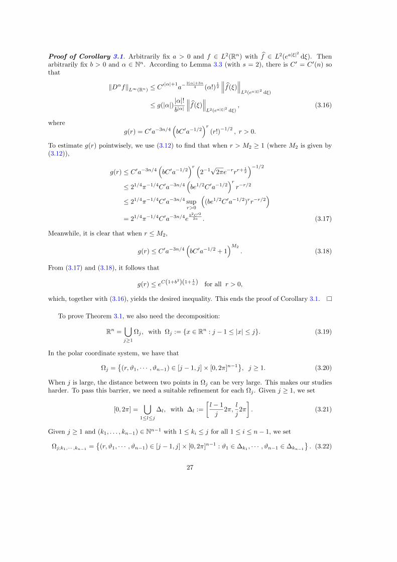
Proof of Corollary 3.1. Arbitrarily fix a > 0 and f ∈ L2(Rn) with f ∈ L2(ea|ξ|2
dξ). Thenarbitrarily fix b > 0 and α ∈ Nn. According to Lemma 3.3 (with s = 2), there is C ′ = C ′(n) sothat
‖Dαf‖L∞(Rn) ≤ C′|α|+1
a−2|α|+3n
4 (α!)12
∥∥∥f(ξ)∥∥∥L2(ea|ξ|2 dξ)
≤ g(|α|) |α|!b|α|
∥∥∥f(ξ)∥∥∥L2(ea|ξ|2 dξ)
, (3.16)
where
g(r) = C ′a−3n/4(bC ′a−1/2
)r(r!)−1/2
, r > 0.
To estimate g(r) pointwisely, we use (3.12) to find that when r > M2 ≥ 1 (where M2 is given by(3.12)),
g(r) ≤ C ′a−3n/4(bC ′a−1/2
)r (2−1√
2πe−rrr+12
)−1/2
≤ 21/4π−1/4C ′a−3n/4(be1/2C ′a−1/2
)rr−r/2
≤ 21/4π−1/4C ′a−3n/4 supr>0
((be1/2C ′a−1/2)rr−r/2
)= 21/4π−1/4C ′a−3n/4e
b2C′22a . (3.17)
Meanwhile, it is clear that when r ≤M2,
g(r) ≤ C ′a−3n/4(bC ′a−1/2 + 1
)M2
. (3.18)
From (3.17) and (3.18), it follows that
g(r) ≤ eC(1+b2)(1+ 1a ) for all r > 0,
which, together with (3.16), yields the desired inequality. This ends the proof of Corollary 3.1.
To prove Theorem 3.1, we also need the decomposition:
Rn =⋃j≥1
Ωj , with Ωj := x ∈ Rn : j − 1 ≤ |x| ≤ j. (3.19)
In the polar coordinate system, we have that
Ωj =
(r, ϑ1, · · · , ϑn−1) ∈ [j − 1, j]× [0, 2π]n−1, j ≥ 1. (3.20)
When j is large, the distance between two points in Ωj can be very large. This makes our studiesharder. To pass this barrier, we need a suitable refinement for each Ωj . Given j ≥ 1, we set
[0, 2π] =⋃
1≤l≤j
∆l, with ∆l :=
[l − 1
j2π,
l
j2π
]. (3.21)
Given j ≥ 1 and (k1, . . . , kn−1) ∈ Nn−1 with 1 ≤ ki ≤ j for all 1 ≤ i ≤ n− 1, we set
Ωj;k1,··· ,kn−1=
(r, ϑ1, · · · , ϑn−1) ∈ [j − 1, j]× [0, 2π]n−1 : ϑ1 ∈ ∆k1 , · · · , ϑn−1 ∈ ∆kn−1
. (3.22)
27

Then one can easily check that for each j ≥ 1,
Ωj;k1,··· ,kn−1
⋂Ωj;k′1,··· ,k′n−1
= ∅, if (k1, · · · , kn−1) 6= (k′1, · · · , k′n−1), (3.23)
and
Ωj =⋃
Ωj;k1,··· ,kn−1, (3.24)
where the union is taken over all different (k1, . . . , kn−1) ∈ Nn−1, with 1 ≤ ki ≤ j for all i =1, . . . , n − 1. It should be mentioned that in the constructions of the decompositions (3.19) and(3.24), we borrowed ideas from [24].
Write |Ωj | (∣∣Ωj;k1,··· ,kn−1
∣∣, resp.) for the volume of Ωj (Ωj;k1,··· ,kn−1, resp.); Write d
(Ωj;k1,··· ,kn−1
)for the diameter of Ωj;k1,··· ,kn−1
. Then we have the following conclusions:Conclusion One. There are constants c1 = c1(n) and c2 = c2(n) so that for any j ≥ 1 and any(k1, . . . , kn−1) ∈ Nn−1, with 1 ≤ ki ≤ j for all i = 1, . . . , n− 1,
c1Vn ≤∣∣Ωj;k1,··· ,kn−1
∣∣ ≤ c2Vn. (3.25)
Conclusion Two. We have that for any j ≥ 1 and any (k1, . . . , kn−1) ∈ Nn−1, with 1 ≤ ki ≤ j forall i = 1, . . . , n− 1,
d(Ωj;k1,··· ,kn−1
)= d (Ωj;1,··· ,1) := sup
x,x′∈Ωj;1,··· ,1
|x− x′|. (3.26)
Conclusion Three. We have that for any fix j ≥ 1 and (k1, . . . , kn−1) ∈ Nn−1, with 1 ≤ ki ≤ j <j + 1 for all i = 1, . . . , n− 1,
d(Ωj;k1,··· ,kn−1
)≤ 2π
√ ∑1≤i≤n
i2 ≤ 2πn32 ; (3.27)
d(Ωj+1;k1,··· ,kn−1
)≤ 2π
j + 1
j
√ ∑1≤i≤n
i2 ≤ 4πn32 . (3.28)
We now explain why the above conclusions are true.To see Conclusion One, we use the definitions of Ωj+1;k1,··· ,kn−1 and Ωj to find that∣∣Ωj;k1,··· ,kn−1
∣∣ =1
jn−1|Ωj | = Vn
jn − (j − 1)n
jn−1,
which leads to (3.25).Conclusion Two follows immediately from the definitions of Ωj;k1,··· ,kn−1
and d(Ωj;k1,··· ,kn−1
).
To show (3.27) in Conclusion Three, we let (r, ϑ1, · · · , ϑn−1) and (r, ϑ′1, · · · , ϑ′n−1) be the polarcoordinates of x = (x1, . . . , xn) and x′ = (x′1, . . . , x
′n), respectively. Then we have that
x, x′ ∈ Ωj;1,··· ,1 ⇐⇒ j − 1 ≤ r ≤ j, 0 ≤ ϑl, ϑ′l ≤2π
jfor all l = 1, · · · , n− 1. (3.29)
Notice that the connection between (x1, . . . , xn) and (r, ϑ1, . . . , ϑn−1) is as:
x1 = r cosϑ1,
x2 = r sinϑ1 cosϑ2,
· · ·xn−1 = r sinϑ1 sinϑ2 · · · sinϑn−2 cosϑn−1,
xn = r sinϑ1 sinϑ2 · · · sinϑn−2 sinϑn−1.
28

Then, by the mean value theorem, we have that for some ζ ∈ (0, 2π/j),
|x1 − x′1| = r| cosϑ1 − cosϑ′1| = r| sin ζ · (ϑ1 − ϑ′1)| ≤ j| sin ζ|2πj≤ 2π.
By inserting suitable terms and using the mean value theorem, we have that
|x2 − x′2| ≤ r(| sinϑ1 cosϑ2 − sinϑ1 cosϑ′2|+ | sinϑ1 cosϑ′2 − sinϑ′1 cosϑ′2|
)≤ 2π · 2.
Similarly, we can verify that
|xi − x′i| ≤ 2π · i for all i = 3, . . . , n.
These, along with (3.26), leads to (3.27).The inequality (3.28) in Conclusion Three can be proved in the same way. The reason that the
factor j+1j appears in (3.28) is as follows: Since 1 ≤ ki ≤ j < j+ 1 (for all i = 1, . . . , n− 1), we see
from the definition of Ωj+1;1,··· ,1 that
x, x′ ∈ Ωj+1;1,··· ,1 ⇐⇒ j ≤ r ≤ j + 1, 0 ≤ ϑl, ϑ′l ≤2π
jfor all l = 1, · · · , n− 1.
(The above is comparable with (3.29).)In summary, we conclude that the above three conclusions are true.
To prove Theorem 3.1, we also need the next lemma concerning with the propagation of forreal-analytic functions.
Lemma 3.4. There are constants C = C(n) > 0 and θ = θ(n) ∈ (0, 1) so that for any a > 0 andj ≥ 1, and for all (k1, . . . , kn−1) ∈ Nn−1, with 1 ≤ ki ≤ j (i = 1, . . . , n− 1),∫
Ωj+1;k1,··· ,kn−1
|f |2 dx ≤ eC(1+ 1a )(∫
Ωj;k1,··· ,kn−1
|f |2 dx)θ(∫
Rn|f |2ea|ξ|
2
dξ)1−θ
,
when f ∈ L2(Rn) satisfies that f ∈ L2(ea|ξ|2
dξ).
The proof of Lemma 3.4 needs Corollary 3.1 and the next lemma which is quoted from [1] (seealso [2, Theorem 4]), but is originally from [51].
Lemma 3.5 ([1, Theorem 4] Sec. 3). Let R > 0 and let f : B2R ⊂ Rn → R be real analytic inB2R verifying
|Dαf(x)| ≤M(ρR)−|α||α|!, when x ∈ B2R and α ∈ Nn
for some positive numbers M and ρ ∈ (0, 1]. Let ω ⊂ BR be a subset of positive measure. Thenthere are two constants C = C(ρ, |ω|/|BR|) > 0 and θ = θ(ρ, |ω|/|BR|) ∈ (0, 1) so that
‖f‖L∞(BR) ≤ CM1−θ( 1
|ω|
∫ω
|f(x)| dx)θ.
We now on the position to show Lemma 3.4.
Proof of Lemma 3.4. Let a > 0 and j ≥ 1 be arbitrarily given. Arbitrarily fix (k1, . . . , kn−1) ∈Nn−1, with 1 ≤ ki ≤ j for all i = 1, . . . , n − 1, and then arbitrarily fix f ∈ L2(Rn) with f ∈L2(ea|ξ|
2
dξ). Since Ωj;k1,··· ,kn−1
⋃Ωj+1;k1,··· ,kn−1
is connected (see (3.22)), it follows from (3.27)and (3.28) that
d(
Ωj;k1,··· ,kn−1
⋃Ωj+1;k1,··· ,kn−1
)≤ d
(Ωj;k1,··· ,kn−1
)+ d
(Ωj+1;k1,··· ,kn−1
)≤ 6πn
32 .
29

Thus, there exists x ∈ Rn such that
Ωj;k1,··· ,kn−1
⋃Ωj+1;k1,··· ,kn−1
⊂ BR0(x), with R0 = 3πn
32 . (3.30)
According to Corollary 3.1 where b = R0, there is C = C(n) > 0 such that for all α ∈ Nn,
‖Dαf‖L∞(Rn) ≤ eC(1+ 1
a ) |α|!R|α|0
∥∥∥f(ξ)∥∥∥L2(ea|ξ|2 dξ)
. (3.31)
By (3.31), as well as (3.30), we can apply Lemma 3.5, where
ρ = 1, R = R0, BR = BR0(x), B2R = B2R0
(x), ω = Ωj;k1,··· ,kn−1, M = eC(1+ 1
a )∥∥∥f(ξ)
∥∥∥L2(ea|ξ|2 dξ)
,
to find constants C0 = C0(n) > 0 and θ = θ(n) ∈ (0, 1) so that
‖f‖L2(BR0(x)) ≤ C0‖f‖θL2(Ωj;k1,··· ,kn−1)
(eC(1+ 1
a )∥∥∥f(ξ)
∥∥∥L2(ea|ξ|2 dξ)
)1−θ
≤ C0eC(1+ 1
a )‖f‖θL2(Ωj;k1,··· ,kn−1)
∥∥∥f(ξ)∥∥∥1−θ
L2(ea|ξ|2 dξ). (3.32)
(Here, we used (3.25) and a coordinate translation.)Finally, the desired inequality of the lemma follows from (3.32) and (3.30). This ends the proof
of Lemma 3.4.
Based on Lemma 3.4, we can have the next propagation result which will be used later.
Lemma 3.6. There exist constants C = C(n) > 0 and θ = θ(n) ∈ (0, 1) so that for any a > 0 andj ≥ 1, ∫
Ωj+1
|f |2 dx ≤ jn−1eC(1+ 1a )(∫
B1
|f |2 dx)θj(∫
Rn|f |2ea|ξ|
2
dξ)1−θj
,
when f ∈ L2(Rn) satisfies that f ∈ L2(ea|ξ|2
dξ).
Proof. Arbitrarily fix a > 0 and j ≥ 1. And then arbitrarily fix f ∈ L2(Rn) with f ∈ L2(ea|ξ|2
dξ).From (3.23) and (3.24), we see that Ωj is the disjoint union of all Ωj;k1,··· ,kn−1
with different(k1, . . . , kn−1) ∈ Nn−1 satisfying 1 ≤ ki ≤ j for all i = 1, . . . , n − 1. Meanwhile, by (3.20), (3.21)and (3.22), one can also check that Ωj+1 is the disjoint union of all Ωj+1;k1,··· ,kn−1
with different(k1, . . . , kn−1) ∈ Nn−1 satisfying 1 ≤ ki ≤ j for all i = 1, . . . , n− 1. These, along with Lemma 3.4,yield that for some C = C(n) > 0 and θ = θ(n),∫
Ωj+1
|f |2 dx =∑∫
Ωj+1;k1,··· ,kn−1
|f |2 dx
≤∑
eC(1+ 1a )(∫
Ωj;k1,··· ,kn−1
|f |2 dx)θ(∫
Rn|f |2ea|ξ|
2
dξ)1−θ
≤ eC(1+ 1a )(∑∫
Ωj;k1,··· ,kn−1
|f |2 dx)θ(∑∫
Rn|f |2ea|ξ|
2
dξ)1−θ
= j(n−1)(1−θ)eC(1+ 1a )(∫
Ωj
|f |2 dx)θ(∫
Rn|f |2ea|ξ|
2
dξ)1−θ
, (3.33)
30

where the sums are taken over all different (k1, . . . , kn−1) ∈ Nn−1 with 1 ≤ ki ≤ j for all i =1, . . . , n − 1. (Notice that there are jn−1 such (k1, . . . , kn−1)). From (3.33), we can use theinduction method to verify that∫
Ωj+1
|f |2 dx ≤(j(j − 1)θ(j − 2)θ
2
· · · 2θj−2
1θj−1)(n−1)(1−θ)
× eC(1+ 1a )(1+θ+···+θj−1)
(∫Ω1
|f |2 dx)θj(∫
Rn|f |2ea|ξ|
2
dξ)1−θj
≤ jn−1eC
1−θ (1+ 1a )(∫
Ω1
|f |2 dx)θj(∫
Rn|f |2ea|ξ|
2
dξ)1−θj
. (3.34)
Since Ω1 = B1 and θ = θ(n) ∈ (0, 1), the desired conclusion in the lemma follows from (3.34). Thisends the proof of Lemma 3.6.
The next proposition plays a very important role in the proof of Theorem 3.1.
Proposition 3.1. There exist constants C = C(n) > 0 and θ = θ(n) ∈ (0, 1) so that for anya > 0, t > 0 and ε > 0,∫
Rne−a|x||f |2 dx ≤ eC(1+ 1
t+a)(
1 + a−nΓ( a
2| ln θ|
))(ε
∫Rn|f |2et|ξ|
2
dξ + eε− 2| ln θ|
a
∫B1
|f |2 dx),
when f ∈ L2(Rn) satisfies f ∈ L2(et|ξ|2
dξ).
To prove Proposition 3.1, we need the following result quoted from [52]:
Lemma 3.7 ([52, Lemma 3.1]). Let a > 0, b ∈ (0, 1) and θ ∈ (0, 1). Then
∞∑k=1
bθk
e−ak ≤ ea
| ln θ|Γ( a
| ln θ|
)| lnx|−
a| ln θ| .
Proof of Proposition 3.1. Arbitrarily fix a > 0 and t > 0. And then arbitrarily fix f ∈ L2(Rn)
satisfies f ∈ L2(et|ξ|2
dξ). It suffices to show the inequality in Proposition 3.1 for the above fixeda, t, f and any ε > 0. Without loss of generality, we can assume that
A :=
∫Rn|f |2et|ξ|
2
dξ 6= 0 and B :=
∫B1
|f |2 dx 6= 0. (3.35)
For otherwise, when A = 0, we have that f = 0 over Rn, thus the desired inequality is trivial;while when B = 0, we can use the analyticity of f (which follows from Corollary 3.1) to see thatf = 0 over Rn and then the desired inequality is trivial again.
By (3.19), we have that∫Rne−a|x||f |2 dx =
∫B1
e−a|x||f |2 dx+∑j≥1
∫Ωj+1
e−a|x||f |2 dx
≤∫B1
|f |2 dx+∑j≥1
∫Ωj+1
e−aj |f |2 dx. (3.36)
We now estimate the last term of (3.36). According to Lemma 3.6, there is C1 = C1(n) > 0 andθ = θ(n) ∈ (0, 1) so that
∑j≥1
∫Ωj+1
e−aj |f |2 dx ≤ eC1(1+ 1t )∑j≥1
jn−1e−aj(∫
B1
|f |2 dx
)θj (∫Rn|f |2et|ξ|
2
dξ
)1−θj
31

≤ eC1(1+ 1t )n! (2/a)
n∑j≥1
e−a2 jA (B/A)
θj, (3.37)
where A and B are given by (3.35). In the proof of (3.37), we used the inequality:
jne−a2 j ≤ n! (2/a)
nfor all j ≥ 1.
Meanwhile, by Lemma 3.7 (with b = B/A), we have that∑j≥1
e−a2 jA(B/A)θ
j
≤ ea2
| ln θ|Γ( a
2| ln θ|
)A| ln(B/A)|−
a2| ln θ| . (3.38)
About A/B, there are only two possibilities: either A/B > e or A/B ≤ e.In the first case when A/B > e, we claim that
A| ln(B/A)|−a
2| ln θ| ≤ εA+ eε− 2| ln θ|
a B for all ε > 0. (3.39)
In fact, when ε satisfies thatA| ln(B/A)|−
a2| ln θ| ≤ εA,
(3.39) is trivial. One the other hand, when ε > 0 satisfies that
A| ln(B/A)|−a
2| ln θ| > εA,
we have that
A/B < eε− 2| ln θ|
a .
This, along with the fact that A/B > e, yields that
A| ln(B/A)|−a
2| ln θ| ≤ A ≤ B ·A/B ≤ eε− 2| ln θ|
a B for all ε > 0.
Thus, we have proved (3.39).Inserting (3.39) into (3.38) leads to∑
j≥1
e−a2 jA(B/A)θ
j
≤ ea2
| ln θ|Γ( a
2| ln θ|
)(εA+ eε
− 2| ln θ|a B
)for all ε > 0. (3.40)
Now it follows from (3.36),(3.37) and (3.40) that for some C2 = C2(n) > 0,∫Rne−a|x||f |2 dx ≤ eC1(1+ 1
t )n!(1 + (2
a)n
ea2
| ln θ|Γ( a
2| ln θ|))(εA+ eε
− 2| ln θ|a B
)≤ eC2(1+ 1
t+a)(1 + a−nΓ( a
2| ln θ|))(εA+ eε
− 2| ln θ|a B
)for any ε > 0.
This proves the desired inequality for the first case that A/B > e.In the second case where A/B ≤ e, we derive directly that∫
Rne−a|x||f |2 dx ≤
∫Rn|f |2 dx ≤
∫Rn|f |2et|ξ|
2
dξ ≤ e∫B1
|f |2 dx
≤ e(ε
∫Rn|f |2et|ξ|
2
dξ + eε− 2| ln θ|
a
∫B1
|f |2 dx
)for any ε > 0.
This proves the desired inequality for the second case that A/B ≤ e.Hence, we end the proof of Proposition 3.1.
32

We now are on the position to show Theorem 3.1.
Proof of Theorem 3.1. (i). Arbitrarily fix u0 ∈ L2(ea|x|dx). Let u(T, x) = (eT4u0)(x), x ∈ Rn.By the Holder inequality, we have that∫
Rn|u(T, x)|2 dx ≤
(∫Rn|u(T, x)|2ea|x| dx
)1/2(∫Rn|u(T, x)|2e−a|x| dx
)1/2
. (3.41)
We will estimate the two terms on right side of (3.41) one by one. For the first term, we applyLemma 3.1 (with ν = 1) to obtain that∫
Rn|u(T, x)|2ea|x| dx ≤ 2ne2a2T
∫Rn|u0(x)|2ea|x| dx. (3.42)
To estimate the second term (on right side of (3.41)), we first notice that eT∆u0 ∈ L2(eT |ξ|2
dξ),since u0 ∈ L2(ea|x|dx) ⊂ L2(Rn). Thus, we can apply Proposition 3.1 (with f = eT4u0 andt = 2T ) to find C = C(n) > 0 and θ = θ(n) ∈ (0, 1) so that for each ε > 0,∫
Rne−a|x||u(T, x)|2 dx ≤ C(T, a, n)
(ε
∫Rn|u0(x)|2 dx+ eε
− 2| ln θ|a
∫B1
|u(T, x)|2 dx), (3.43)
whereC(T, a, n) = eC(1+ 1
T +a)(
1 + a−nΓ( a
2| ln θ|
)).
Inserting (3.42) and (3.43) into (3.41), we get that for each ε > 0∫Rn|u(T, x)|2 dx ≤ C
(∫Rn|u0(x)|2ea|x| dx
)1/2(ε
∫Rn|u0(x)|2 dx+ eε
− 2| ln θ|a
∫B1
|u(T, x)|2 dx)1/2
≤ C(ε1/2
∫Rn|u0(x)|2ea|x| dx
)1/2(ε1/2
∫Rn|u0(x)|2 dx+ ε−1/2eε
− 2| ln θ|a
∫B1
|u(T, x)|2 dx)1/2
≤ 2−1C(ε1/2
∫Rn|u0(x)|2ea|x| dx+ ε1/2
∫Rn|u0(x)|2 dx+ ε−1/2eε
− 2| ln θ|a
∫B1
|u(T, x)|2 dx)
≤ C(ε1/2
∫Rn|u0(x)|2ea|x| dx+ ε−1/2eε
− 2| ln θ|a
∫B1
|u(T, x)|2 dx), (3.44)
whereC = C(T, a, n) = 2n/2ea
2T√C(T, a, n).
Since ε > 0 can be arbitrary taken, we replace ε by ε2 in (3.44) to get the desired conclusion in (i)of Theorem 3.1.
(ii). Arbitrarily fix u0 ∈ L2(〈x〉νdx). Let u(T, x) =(eT4u0
)(x), x ∈ Rn. Three facts are given
in order. Fact One. Using the inequality:
1 ≤ ε|x|ν + e(1/ε)1ν e−|x| for all ε > 0 and x ∈ Rn,
we find that ∫Rn|u(T, x)|2 dx ≤ ε
∫Rn|u(T, x)|2|x|ν dx+ e(1/ε)
1ν
∫Rn|u(T, x)|2e−|x| dx. (3.45)
Fact Two. Since 0 < ν ≤ 1, we can apply Lemma 3.2 to find C1 = C1(n) so that∫Rn|u(T, x)|2|x|ν dx ≤
(2ν+2Γ(ν/2 + n)
(1 + T
ν4
)‖u0‖L2(〈x〉ν dx)
)2
33

≤ C1
(1 + T
ν2
) ∫Rn|u0(x)|2〈x〉ν dx. (3.46)
Fact Three. We can use Proposition 3.1 (with f = eT4u0, t = 2T and a = 1) to find C2 = C2(n)and θ = θ(n) ∈ (0, 1) so that for all µ > 0,∫
Rne−|x||u(T, x)|2 dx ≤ eC2(1+ 1
T )(µ
∫Rn|u0(x)|2 dx+ eµ
−2| ln θ|∫B1
∣∣(eT4u0
)(x)∣∣2 dx
). (3.47)
To continue the proof, we arbitrarily fix ε > 0. We will first use Fact Three, and then use Fact
One and Fact Two. By taking µ = εe−( 1ε )
1α in (3.47), we obtain that
e(1/ε)1ν
∫Rne−|x||u(T, x)|2 dx
≤ e(1/ε)1ν eC2(1+ 1
T )(µ
∫Rn|u0(x)|2 dx+ eµ
−2| ln θ|∫B1
|u(T, x)|2 dx)
= eC2(1+ 1T )(ε
∫Rn|u0(x)|2 dx+ bε
∫B1
|u(T, x)|2 dx), (3.48)
where
bε = exp[(1/ε)
1ν + (ε−2e2(1/ε)
1ν )| ln θ|
].
Meanwhile, one can directly check the following two inequalities:
s2 ≤ es for all s > 0; (3.49)
s+ e3| ln θ|s ≤ e(3| ln θ|+1)s for all s > 0. (3.50)
Choosing s = ε−1 and s = (1/ε)1ν in (3.49) and (3.50) respectively, using 0 < ν ≤ 1, we find that
bε ≤ exp[(1/ε)
1ν + (e1/εe2(1/ε)
1ν )| ln θ|
]≤ exp
[(1/ε)
1ν + (e3(1/ε)
1ν )| ln θ|
]exp
[(1/ε)
1ν + e3| ln θ|(1/ε)
1ν]
≤ exp[e(3| ln θ|+1)(1/ε)
1ν]. (3.51)
Combining (3.48) and (3.51) leads to that
e(1/ε)1ν
∫Rne−|x||u(T, x)|2 dx
≤ eC2(n)(1+ 1T )(ε
∫Rn|u0(x)|2 dx+ ee
(3| ln θ|+1)(1/ε)1ν∫B1
|u(T, x)|2 dx). (3.52)
Finally, inserting (3.46) and (3.52) into (3.45), we obtain that for some C3 = C3(n),∫Rn|u(T, x)|2 dx
≤(C1(1 + T
ν2 ) + eC2(1+ 1
T ))(ε
∫Rn|u0(x)|2〈x〉ν dx+ ee
(3| ln θ|+1)(1/ε)1ν∫B1
|u(T, x)|2 dx)
≤ (1 + Tν2 )eC3(1+ 1
T )(ε
∫Rn|u0(x)|2〈x〉ν dx+ ee
(3| ln θ|+1)(1/ε)1ν∫B1
|u(T, x)|2 dx),
which leads to the desired conclusion in (ii) of Theorem 3.1.Hence, we end the proof of Theorem 3.1.
34

3.2 Weak observability inequalities with observations on balls
According to Theorem 1.1, it is impossible to recover a solution of (1.1) by observing it over aball. Thus, two interesting questions arise. First, can we recover a solution of (1.1) over a ballby observing it on another ball? Second, can we have observability inequalities with observationsover balls for solutions of (1.1) with some kind of initial values? The answer to the first questionis almost negative, while we give partially positive answer for the second question. The first mainresult of this subsection is stated as follows:
Theorem 3.2. (i) There is an absolute positive constant C so that for all T > 0 and 0 < r′ < r,∫Br′
u2(T, x) dx ≤(
1
T+
Cn
(r − r′)2
)∫ T
0
∫Br
u2(t, x) dx dt, when u solves (1.1).
(ii) Given T > 0 and r′ > r > 0, there is no constant C = C(T, r′, r, n) so that∫Br′
u2(T, x) dx ≤ C∫ T
0
∫Br
u2(t, x) dxdt for any solution u to (1.1).
Proof. (i) Arbitrarily fix T > 0 and 0 < r′ < r. Arbitrarily fix a solution u to (1.1). Letu(0, x) = u0(x), x ∈ Rn. Choose a C2 function ϕ on Rn so that for some absolute constant C > 0,
0 ≤ ϕ(x) ≤ 1 over Rn; |Dαϕ(x)| ≤ C (r − r′)−|α| for all α ∈ Nn, with |α| ≤ 2, (3.53)
and so that
ϕ(x) =
1, x ∈ Br′ ,0, x ∈ Bcr .
Set v = ϕu. Then v satisfies
vt −4v = −2∇ϕ · ∇u−4ϕu in R+ × Rn, v(0, ·) = ϕ(·)u0(·) in Rn. (3.54)
Multiplying (3.54) by tv leads to
1
2
(tv2)t− 1
2v2 − tv4v = −2tu∇ϕ · ∇v + t
(2|∇ϕ|2 − ϕ4ϕ
)u2. (3.55)
Integrating (3.55) over (0, T )× Rn, we have that
1
2
∫RnTv2(T, x) dx− 1
2
∫ T
0
∫Rnv(t, x)2 dx dt+
∫ T
0
∫Rnt |∇v(t, x)|2 dxdt (3.56)
=
∫ T
0
∫Rn−2tu∇ϕ(x) · ∇v(t, x) dx dt
+
∫ T
0
∫Rnt(
2 |∇ϕ(x)|2 − ϕ(x)4ϕ(x))u2(t, x) dx dt.
Meanwhile, by the Holder inequality, we find that∣∣∣ ∫ T
0
∫Rn−2tu(t, x)∇ϕ(x) · ∇v(t, x) dxdt
∣∣∣≤∫ T
0
∫Rnt |∇v(t, x)|2 dxdt+
∫ T
0
∫Rnt |∇ϕ(x)|2 u2(t, x) dx dt. (3.57)
35

Inserting (3.57) into (3.56) leads to that
T
∫Rnv2(T, x) dx
≤∫ T
0
∫Rnv2(t, x) dxdt+ 2
∫ T
0
∫Rnt(3|∇ϕ(x)|2 − ϕ(x)4ϕ(x)
)u2(t, x) dxdt. (3.58)
Since v = u on Br′ and v = 0 on Bcr , we can use (3.58) and (3.53) to get that∫Br′
u2(T, x) dx
≤ 1
T
∫ T
0
∫Br
u2(t, x) dxdt+2
T
∫ T
0
∫Br\Br′
t(3|∇ϕ(x)|2 − ϕ(x)4ϕ(x)
)u2(t, x) dx dt
≤(
1
T+
8Cn
(r − r′)2
)∫ T
0
∫Br
u2(t, x) dxdt,
which leads to the desired conclusion in (i) of Theorem 3.2.
(ii) By contradiction, we suppose that there were T > 0, r′ > r > 0 and C = C(T, r′, r, n) > 0so that ∫
Br′
u2(T, x) dx ≤ C∫ T
0
∫Br
u2(t, x) dxdt for any solution u to (1.1). (3.59)
We would use a constructive method to derive a contradiction with (3.59). For this purpose, wedefine, for each k ≥ 1,
uk(t, x) =1
(4π(t+ 1))n/2e−|x1−k|
2+|x′|24(t+1) , (t, x) = (t, x1, x
′) ∈ [0,∞)× R× Rn−1.
One can easily check that uk is the solution of (1.1) with initial value:
uk(0, x) =1
(4π)n/2e−|x1−k|
2+|x′|24 , x = (x1, x
′) ∈ R× Rn−1.
It is clear that uk(0, ·)k≥1 is uniformly bounded in L2(Rn).We next show that when k is large enough, uk does not satisfy (3.59) (which leads to a contra-
diction). To this end, we need two estimates:∫ T
0
∫Br
u2k(t, x) dxdt ≤ rnTVn
(4π(T + 1))ne−
(k−r)22(T+1) , when k is large enough; (3.60)
∫Br′
u2k(T, x) dx ≥ 1
(4π(T + 1))ne−
(k−r−σ3
)2
2(T+1) (σ/3)nVn, when k is large enough. (3.61)
To show (3.60), we obtain from a direct computation that
∂t(lnuk(t, x)) = −n2
1
t+ 1+|x1 − k|2 + |x′|2
4(t+ 1)2for all t ≥ 0, x = (x1, x
′) ∈ Rn,
from which, it follows that when t ≥ 0 and x = (x1, x′) ∈ Rn,
∂t(lnuk(t, x)) > 0⇐⇒ |x1 − k|2 + |x′|2 > 2n(t+ 1).
36

This implies that
k > r +√
2n(T + 1) =⇒ ∂t(lnuk(t, x)) > 0 for all (t, x)× (0, T )×Br.
From the above, we see that when k > r +√
2n(T + 1), we have that for each x ∈ Br, uk(t, x) is
an increasing function of t on [0, T ]. Hence, when k > r +√
2n(T + 1),∫ T
0
∫Br
u2k(t, x) dx dt ≤
∫ T
0
∫Br
u2k(T, x) dxdt =
∫ T
0
∫Br
1
(4π(T + 1))ne−|x1−k|
2+|x′|22(T+1) dx dt
=T
(4π(T + 1))n
∫Br
e−|x1−k|
2+|x′|22(T+1) dx ≤ T
(4π(T + 1))n
∫Br
e−|k−r|22(T+1) dx
≤ rnTVn(4π(T + 1))n
e−(k−r)22(T+1) ,
which leads to (3.60).We next show (3.61). Given b > 0, use Br(b, 0
′) to denote the ball centered at (b, 0, 0, · · · , 0)and of radius r, namely
Br(b, 0′) :=
x ∈ Rn : |x1 − b|2 + |x′|2 ≤ r2
.
Let k > r′ and σ = r′ − r. Then∫Br′
u2k(T, x) dx ≥
∫Br′
⋂Bk−r−σ
3(k,0′)
u2k(T, x) dx
=
∫Br′
⋂Bk−r−σ
3(k,0′)
1
(4π(T + 1))ne−|x1−k|
2+|x′|22(T+1) dx
≥ 1
(4π(T + 1))ne−
(k−r−σ3 )2
2(T+1)
∣∣∣Br′⋂Bk−r−σ3 (k, 0′)∣∣∣ . (3.62)
Meanwhile, it is clear that
Bσ3(r + 2σ/3, 0′) ⊂ Br′
⋂Bk−r−σ3 (k, 0′),
which leads to that ∣∣∣Br′⋂Bk−r−σ3 (k, 0′)∣∣∣ ≥ ∣∣Bσ
3(r + 2σ/3, 0′)
∣∣ = (σ/3)nVn. (3.63)
Now (3.61) follows from (3.62) and (3.63) at once.From (3.60) and (3.61), we find that when k > maxr +
√2n(T + 1), r′,∫ T
0
∫Br
u2k(t, x) dx dt∫
Br′
u2k(T, x) dx
≤rnTVn
(4π(T+1))n e− (k−r)2
2(T+1)
1(4π(T+1))n e
− (k−r−σ3 )2
2(T+1)(σ3
)nVn
= T(3r
σ
)ne
12(T+1)
((k−r−σ3 )
2−(k−r)2)
= T(3r
σ
)ne
12(T+1) ((σ3 )2− 2σ
3 (k−r))
= T( 3r
r′ − r
)ne
12(T+1)
((r′−r
3
)2− 2r′−r
3 (k−r)). (3.64)
37

Since
(r′ − r
3)2 − 2r′ − r
3(k − r)→ −∞,
we see from (3.64) that
limk→+∞
∫ T
0
∫Br
u2k(t, x) dx dt∫
Br′
u2k(T, x) dx
= 0,
from which, it follows that uk does not satisfy (3.59), when k is large enough. This shows theconclusion in (ii) of Theorem 3.2.
Hence, we end the proof of Theorem 3.2.
The next corollary is a direct consequence of Theorem 3.2.
Corollary 3.2. Given ν > 0, T > 0 and r > 0, there is no constant C = C(T, r, ν, n) > 0 so that∫Rnu2(T, x)ρ(x) dx ≤ C
∫ T
0
∫Br
u2(t, x) dxdt for any u solves (1.1), (3.65)
where either ρ(x) = 〈x〉−ν , x ∈ Rn, or ρ(x) = e−|x|, x ∈ Rn.
Remark 3.5. It was announced in [8, p. 384] (without proof) that given a bounded interval E,there is no positive weight function ρ such that∫ ∞
0
|u(T, x)|2ρ(x) dx ≤ C∫ T
0
∫E
|u(t, x)|2 dx dt
for all solutions of the heat equation in the physical space (0,∞). The above Corollary 3.2 presentsa similar result for the heat equation in the physical space Rn.
The second main result of this subsection is stated as follows:
Theorem 3.3. (i) There is a generic constant C so that for any T > 0, M > r > 0 and u0 ∈L2(Rn) with supp u0 ⊂ Br,∫
Rn|u(T, x)|2 dx ≤
(1
T+
Cn
(M − r)2
)∫ T
0
∫BM
|u(t, x)|2 dx dt,
where u is the solution to (1.1) with u(0, ·) = u0(·).
(ii) Assume that 0 ≤ u0 ∈ L1(Rn) so that∫Br
u0(x) dx ≥ µ∫Rnu0(x) dx for some r > 0 and µ ∈ (0, 1).
Then for any T > 0, M > 0 and any solution u to (1.1) with u(0, ·) = u0(·),∫Rn|u(T, x)|2 dx ≤ 2
n2 +1π
n2 T
n2−1
Vn(r ∧M)nµ2e
4r2
T
∫ T
0
∫BM
|u(t, x)|2 dxdt.
Here, r ∧M := minr,M.
38

Proof. (i) The proof is similar to that of (i) of Theorem 3.2. Arbitrarily fix T > 0, M > r > 0 andu0 ∈ L2(Rn) with supp u0 ⊂ Br. Write u for the solution to (1.1) with u(0, ·) = u0(·). Choose aC2 function ϕ over Rn so that for some absolute constant C > 0,
0 ≤ ϕ(x) ≤ 1 over Rn; |Dαϕ(x)| ≤ C(r − r′)−|α| for all α ∈ Nn, with |α| ≤ 2 (3.66)
and so that
ϕ(x) =
0, x ∈ Br,1, x ∈ BcM .
Set v = ϕu. Multiplying (3.54) by v, we find that
1
2
(v2)t− v4v = −2u∇ϕ · ∇v +
(2|∇ϕ|2 − ϕ4ϕ
)u2. (3.67)
Integrating (3.67) over (0, T )× Rn, we obtain that
1
2
∫Rnv2(T, x) dx− 1
2
∫Rnv2(0, x) dx+
∫ T
0
∫Rn|∇v(t, x)|2 dxdt (3.68)
=
∫ T
0
∫Rn−2u(t, x)∇ϕ(x) · ∇v(t, x) dxdt+
∫ T
0
∫Rn
(2|∇ϕ(x)|2 − ϕ(x)4ϕ(x)
)u2(t, x) dx dt.
Since the support of u0 is contained in Br, we have that v(0, ·) = 0 over Rn. Then by the Holderinequality, we deduce from (3.68) that∫
Rnv2(T, x) dx ≤
∫ T
0
∫Rn
2(3|∇ϕ(x)|2 − ϕ(x)4ϕ(x)
)u2(s, x) dxds. (3.69)
Note that (3.69) is still true if we replace T by any t ∈ (0, T ). This implies that∫ T
0
∫Rnv2(t, x) dx dt ≤
∫ T
0
∫ t
0
∫Rn
2(3|∇ϕ(x)|2 − ϕ(x)4ϕ(x)
)u2(t, x) dxdτ dt. (3.70)
Since v = u on BcM , it follows from (3.66) and (3.70) that∫ T
0
∫|x|≥M
u2(t, x) dx ≤ CnT
(M − r)2
∫ T
0
∫r≤|x|≤M
u2(t, x) dxdt. (3.71)
Meanwhile, it is clear that ∫Rnu2(T, x) dx ≤ 1
T
∫ T
0
∫Rnu2(t, x) dxdt. (3.72)
Combining (3.71) and (3.72), we obtain that∫Rnu2(T, x) dx ≤ 1
T
∫ T
0
∫|x|≤M
u2(t, x) dxdt+1
T
∫ T
0
∫|x|≥M
u2(t, x) dx dt
≤ 1
T
∫ T
0
∫|x|≤M
u2(t, x) dxdt+1
T
CnT
(M − r)2
∫ T
0
∫r≤|x|≤M
u2(t, x) dxdt
≤(
1
T+
Cn
(M − r)2
)∫ T
0
∫|x|≤M
u2(t, x) dxdt.
39

which leads to the conclusion (i) of Theorem 3.3.
(ii) Let T > 0 and M > 0 be arbitrarily given. Arbitrarily fix u0 so that
0 ≤ u0 ∈ L1(Rn);
∫Br
u0(x)dx ≥ µ∫Rnu0(x)dx for some r > 0 and µ ∈ (0, 1). (3.73)
Write u for the solution to (1.1) with u(0, ·) = u0(·).We first prove that when 0 < M ≤ r,∫
Rn|u(T, x)|2 dx ≤ 2
n2 +1π
n2 T
n2−1
VnMnµ2e
4r2
T
∫ T
0
∫BM
|u(t, x)|2 dx dt. (3.74)
For this purpose, we need the following two estimates:∫ T
T2
∫|x|≤M
u2(t, x) dxdt ≥ 2−1(4π)−nVnMnµ2T−(n−1)e−
4r2
T
(∫Rnu0(x) dx
)2
; (3.75)
∫Rnu2(T, x) dx ≤ 2−
3n2 (πT )−n/2
(∫Rnu0(x) dx
)2
. (3.76)
To show (3.75), we observe that
u(t, x) =
∫Rn
(4πt)−n/2e−|x−y|2
4t u0(y) dy, (t, x) ∈ (0,∞)× Rn. (3.77)
By (3.77) and (3.73), we find that when t > 0, |x| ≤ r,
u(t, x) ≥∫|y|≤r
(4πt)−n/2e−|x−y|2
4t u0(y) dy ≥∫|y|≤r
(4πt)−n/2e−r2
t u0(y) dy
≥ µ(4πt)−n/2e−r2
t
∫Rnu0(x) dx. (3.78)
Since M ≤ r, it follows from (3.78) that∫ T
T2
∫|x|≤M
u2(t, x) dxdt ≥ VnMnµ2
(∫Rnu0(x) dx
)2 ∫ T
T2
(4πt)−ne−2r2
t dt
≥ 2−1(4π)−nVnMnµ2T−(n−1)e−
4r2
T
(∫Rnu0(x) dx
)2
,
which leads to (3.75).We now show (3.76). By (3.77) and the Young inequality, we have that
‖u(T, x)‖L2(Rn) ≤∥∥∥(4πT )−n/2e−
|x|24T
∥∥∥L2(Rn)
∫Rnu0(x) dx = 2−
3n4 (πT )−n/4
∫Rnu0(x) dx,
which leads to (3.76).Next, by (3.75) and (3.76), we see that∫
Rnu2(T, x) dx ≤ 2
n2 +1π
n2 T
n2−1
VnMnµ2e
4r2
T
∫ T
T2
∫|x|≤M
u2(t, x) dxdt
40

≤ 2n2 +1π
n2 T
n2−1
VnMnµ2e
4r2
T
∫ T
0
∫|x|≤M
u2(t, x) dxdt,
which leads to (3.74) for the case when 0 < M ≤ r.Finally, when M > r, we apply (3.74) (with M = r) to obtain that∫
Rnu2(T, x) dx ≤ 2
n2 +1π
n2 T
n2−1
Vnrnµ2e
4r2
T
∫ T
0
∫|x|≤r
u2(t, x) dx dt
≤ 2n2 +1π
n2 T
n2−1
Vnrnµ2e
4r2
T
∫ T
0
∫|x|≤M
u2(t, x) dxdt,
which leads to (3.74) for the case that M > r. So the conclusion (ii) in Theorem 3.3 is true.Hence, we end the proof of Theorem 3.3
Acknowledgment. This work was partially supported by the National Natural Science Foun-dation of China under grants 11501424 and 11701535.
References
[1] J. Apraiz, L. Escauriaza. Null-control and measurable sets. ESAIM: COCV, 19 (2013), 239–254.
[2] J. Apraiz, L Escauriaza, G. Wang, C. Zhang. Observability inequalities and measurable sets.J. Eur. Math. Soc., 16 (2014), 2433–2475.
[3] V. Barbu. Exact null internal controllability for the heat equation on unbounded convexdomains. ESAIM: COCV, 20 (2014), 222–235.
[4] C. Bardos, G. Lebeau, J. Rauch. Sharp sufficient conditions for the observation, control, andstabilization of waves from the boundary. SIAM J. Control and Optim., 30 (1992), 1024–1065.
[5] A. Bonami, B. Demange. A survey on uncertainty principles related to quadratic forms. Col-lect. Math., (2006), 1–36.
[6] N. Burq, R. Joly. Exponential decay for the damped wave equation in unbounded domains.Commun. Contemp. Math., 18 (2016), 1650012.
[7] V. R. Cabanillas, S. B. de Menezes, E. Zuazua. Null controllability in unbounded domains forthe semilinear heat equation with nonlinearities involving gradient terms. J. Optimiz. TheoryApp., 110 (2001), 245–264.
[8] P. Cannarsa, P. Martinez, J. Vancostenoble. Null controllability of the heat equation in un-bounded domains by a finite measure control region. ESAIM: COCV, 10 (2004): 381–408.
[9] T. Duyckaerts, L. Miller. Resolvent conditions for the control of parabolic equations. J. Funct.Anal., 263 (2012), 3641–3673.
[10] S. Ervedoza. Control and stabilization properties for a singular heat equation with an inverse-square potential. Commun. Partial Diff. Eq., 33 (2008), 1996–2019.
[11] L. Escauriaza, F. J. Fernandez, S. Vessella. Doubling properties of caloric functions. Appl.Anal., 85 (2006), 205–223.
41

[12] L. Escauriaza, C. Kenig, G. Ponce, L. Vega. On uniqueness properties of solutions ofSchrodinger equations. Commun. Partial Diff. Eq., 31 (2006), 1811–1823.
[13] L. Escauriaza, C. Kenig, G. Ponce, L. Vega. Hardy’s uncertainty principle, convexity andSchrodinger evolutions. J. Eur. Math. Soc. 10 (2008), 883–907.
[14] L. Escauriaza, C. Kenig, G. Ponce, L. Vega. Uniqueness properties of solutions to Schrodingerequations. Bull. Amer. Math. Soc. 49 (2012), 415–442.
[15] L. Escauriaza, C. E. Kenig, G. Ponce and L. Vega. Hardy Uncertainty Principle, Convexityand Parabolic Evolutions, Commun. Math. Phys. 346 (2016) 667–678.
[16] L. Escauriaza, S. Montaner, C. Zhang. Observation from measurable sets for parabolic analyticevolutions and applications. J. Math. Pures Appl, 104 (2015): 837–867.
[17] G. B. Folland, A. Sitaram. The uncertainty principle: a mathematical survey. J. Fourier Anal.Appl., 3 (1997), 207–238.
[18] A. V. Fursikov, O. Y. Imanuvilov. Controllability of evolution equations. Seoul National Uni-versity, 1996.
[19] V. Havin, B. Joricke. The Uncertainty Principle in Harmonic Analysis. Springer Science &Business Media, 2012.
[20] A. Ionescu, C. Kenig. Lp Carleman inequalities and uniqueness of solutions of nonlinearSchrodinger equations. Acta Math. 193 (2004), 193–239.
[21] A. Ionescu, C. Kenig. Uniqueness properties of solutions of Schrodinger equations. J. Funct.Anal., 232 (2006), 90–136.
[22] R. Joly, C. Laurent. Stabilization for the semilinear wave equation with geometric controlcondition. Analysis & PDE, 6 (2013), 1089–1119.
[23] V. E. Kacnelson. Equivalent norms in spaces of entire functions. Mathematics of the USSR-Sbornik, 21 (1973), 33.
[24] O. Kovrijkine. Some results related to the Logvinenko-Sereda theorem. Proc. Amer. Math.Soc., 129 (2001), 3037–3047.
[25] S. Huang, A. Soffer. Uncertainty principle, minimal escape velocities and observability in-equalities for schro dinger equations. arXiv:1709.09485, 2017.
[26] C. Laurent. Internal control of the Schrodinger equation. Math. Control Relat. F., 4 (2014),161–186.
[27] G. Lebeau, L. Robbiano. Controle exact de lequation de la chaleur. Commun. Partial Diff.Eq., 20 (1995), 335–356.
[28] G. Lebeau and E. Zuazua, Null-controllability of a system of linear thermoelasticity, Arch.Rational Mech. Anal., 141 (1998), pp. 297-329.
[29] J. Le Rousseau, G. Lebeau, P. Terpolilli, E. Trelat. Geometric control condition for the waveequation with a time-dependent observation domain. Analysis & PDE, 10 (2017), 983–1015.
[30] J. Le Rousseau, I. Moyano. Null-controllability of the Kolmogorov equation in the whole phasespace. J. Differ. Equ., 260 (2016), 3193–3233.
42

[31] V. N. Logvinenko, J. F. Sereda. Equivalent norms in spaces of entire functions of exponentialtype. Teor. FunkciiFunkcional. Anal. i Prilozen. Vyp, 20 (1974), 102–111.
[32] A. Lopez, X. Zhang, and E. Zuazua. Null controllability of the heat equation as singular limitof the exact controllability of dissipative wave equations, J. Math. Pures Appl., 79 (2000),741–808.
[33] Q. Lu. A lower bound on local energy of partial sum of eigenfunctions for Laplace-Beltramioperators. ESAIM COCV, 19 (2013) 255–273.
[34] Q. Lu, Z. Yin. Unique continuation for stochastic heat equations. ESAIM: COCV, 21 (2015),378–398.
[35] S. Micu, E. Zuazua. On the lack of null-controllability of the heat equation on the half-line.Trans. Amer. Math. Soc., 353 (2001), 1635–1659.
[36] S. Micu, E. Zuazua. On the lack of null-controllability of the heat equation on the half space.Port. Math., 58 (2001), 1–24.
[37] L. Miller. On the null-controllability of the heat equation in unbounded domains. B. Sci.math., 129 (2005), 175–185.
[38] L. Miller. Unique continuation estimates for the Laplacian and the heat equation on non-compact manifolds. Math. Res. Lett., 12 (2005), 37–47.
[39] L. Miller. Unique continuation estimates for sums of semiclassical eigenfunctions and null-controllability from cones, Preprint, 2009.
[40] F. L. Nazarov. Local estimates for exponential polynomials and their applications to inequal-ities of the uncertainty principle type, Algebra i Mathematicheskiy Analiz 5 (1993), 3–66.
[41] B.P. Paneyah. Some estimates of functions of exponential type and apriori estimates for gern-eral dikerential operators, Uspekhi mat.nauk 21 N3 (1996) 75-114 (Russian).
[42] B.P. Paneyah. On some theorems of Paley-Wiener type. Doklady AN SSSR 138 N1 (1961)47-50 (Russian).
[43] K. D. Phung, G. Wang. Quantitative unique continuation for the semilinear heat equation ina convex domain. J. Funct. Anal., 259 (2010), 1230–1247.
[44] K. D. Phung, G. Wang. An observability estimate for parabolic equations from a measurableset in time and its applications. J. Eur. Math. Soc, 15 (2013), 681–703.
[45] K. D. Phung, G. Wang, Y. Xu. Impulse output rapid stabilization for heat equations. J. Diff.Equ., 263 (2017), 5012–5041.
[46] K. D. Phung, L. Wang, C. Zhang. Bang-bang property for time optimal control of semilinearheat equation. Ann. Inst. H. Poincar’e Anal. Non Lineaire, 31 (2014), 477–499.
[47] J. Rauch, M. Taylor. Exponential decay of solutions to hyperbolic equations in boundeddomains. Indiana Univ. Math. J. 24 (1974), 79–86.
[48] M. Reed and B. Simon. Methods of Modern Mathematical Physics I: Functional Analysis,Academic Press, 1980.
43

[49] A. Reznikov. Sharp constants in the PaneyahCLogvinenkoCSereda theorem. Comptes RendusMathematique, 348 (2010), 141–144.
[50] B. Simon. Schrodinger semigroups. Bull. Amer. Math. Soc., 7 (1982), 447–526.
[51] S. Vessella. A continuous dependence result in the analytic continuation problem. ForumMath. 11, 6 (1999) 695-703.
[52] G. Wang, M. Wang, Y. Zhang. Observability and unique continuation inequalities for theSchrodinger equation. To appear in J. Eur. Math. Soc., arXiv preprint arXiv:1606.05861,2016.
[53] G. Wang, C. Zhang. Observability inequalities from measurable sets for some abstract evolu-tion equations. SIAM J. Control Optim., 55 (2017), 1862–1886.
[54] C. Zhang. Quantitative unique continuation for the heat equation with Coulomb potentials.arXiv preprint arXiv:1707.07744, 2017.
[55] Y. Zhang. Unique continuation estimates for the Kolmogorov equation in the whole space.Comptes Rendus Mathematique, 354 (2016), 389–393.
[56] E. Zuazua. Exponential decay for the semilinear wave equation with localized damping inunbounded domains. J. Math. Pures Appl, 70 (1991), 513–529.
44