Calhoun: The NPS Institutional Archive

Faculty and Researcher Publications Faculty and Researcher Publications

1996-06

Fast interpolation for Global Positioning

System (GPS) Satellite Orbits

Neta, Beny

http://hdl.handle.net/10945/39469

FAST INTERPOLATION FOR GLOBAL POSITIONING SYSTEM (GPS) SATELLITE

ORBITS

Beny Neta Naval Postgraduate School

Department of Mathematics Code MA/Nd

Monterey, CA 93943

D. A. Danielson Naval Postgraduate School

Department of Mathematics Code MA/Dd

Monterey, CA 93943

C. P. Sagovac 819 South Charles Street

Baltimore, MD 21230-3938

J. R. Clynch Naval Postgraduate School

Department of Oceanography Code OC/CI

Monterey, CA 93943

.Tune 2, 1996

Abstract

In Lhis reporL, we discuss and compare several methods for polynomial interpolation of Global Posi­tioning System ephemeris data. We show that the 11se of diirerence Lables is more efficient. than the meLhod currently in use to construct and evaluate the La­grange poly nomiab.

Introdudion

The problem of inLerpolaLing C lob al PosiLioning System (GPS) precise, post fit ephemeris data is :rn important aspect of geodetic work utili :>:ing G PS. Given that a high accuracy ( < 1 m ) , high precision ( 1 cm) or hit can be generated tho11gh the 11se of dense observaLiom and special int.egra.Lions, it. is necessary to interpolate these ephemeris at high accuracy to 11tili:>:e these orbits.

These high accuracy orbits arc produced by several organi:>:ations (D\·1 :\, \JGS, .J PL, several Lniversities) and are widely available. An ephemeris Lypically con­sists of satellite positions at evenly spaced times over a week. Most. ephemeris a.re given at. 900 sec (1.:J min) time steps although the ~GS ones arc at 1200 sec (20 min). The G PS satellites are in 12 hr circ11 lar or hits making 900 sec ephemeris steps 7 .i) deg of a.re.

The typical geodetic user collects G PS data at in­Lerva.b from 1 sec Lo :10 sec and needs Lo find the satellite position at the times of that data. The times needed are really not the evenly spaced received Limes, but. Lhe LransmiL times LhaL a.re about. ()() msec before reception. A precise value for this propaga­Lion delay is not. known unLil the soluLion process is partially done. Therefore usually one needs to find a d11ster of satellite positions a few msec from a nomi­nal evenly spaced interval.

In the past the typical technique used by the Dl"1A [J\falys, Hl8D], l\GS [K.emondi, HH.ll], .J PL [\Vatkins, 1995] and others is a Lagrange interpolation. The orders vary from 81" to 11 11'. This approach directly compuLes the value of Lhe funcLion ( Lhe Lhree CarLe­sian Earth centered earth fixed coordinates) from the 11niq11e polynomial going thro11gh the data points. The coefficients arc not found, and finding them may introd11ce errors [Press et al, HH.l2]. Several eval11a­Liom of the accuracy of Lhis met.hod [Hemondi, 1991, Smith and Curtis, 1983] have been made. It is gencr­a lly fo11nd that an 81

" order Lagrangian interpolation using 900 sec data with the unknown in the center of the points gives val11es that compare with rn1merical inLegraLion a.L Lhe 1 cm level.

The problem addressed here is to find if a more ef­ficient n11merica l met hod th at achieves the same ac­curacy can be used. This is moLiva.Led by Lhe move-

0 50 100 150 200 250 300 350 4002.5

2

1.5

1

0.5

0

0.5

1

1.5

2

2.5x 104

point number (time)

Earth

fixed

xco

ordi

nate

(km

)

GPS ephemeris data (4 days)

time period, we have the opportunity to "front load" our work ::it the tinw of ephemeris receipt. Ky cal­culating neede<l data in a.d vance we should be able to shorten the real time operation count. Thus we will be more concerned with the rapid evalua.Lion of intcrpolants for specific times than their rapid gener­ation. Of course in some cases the times of ev::i luation and generation will be closely rela.Le<l, as mentioned above. In others, they will be quite different and our hope will be Lo shifL as much of the work as possi­ble to the generation of efficient intcrpolants so as to ::i llow the r~1pid evahrntion of those interpol ants.

In summary, we will describe the following met.h­ods:

• La.grange polynomial int.erpola.Lion

• ~cwton's divided difference interpolation poly­nomial

• Diirerence Tables

• Cubic Spline interpolation

• 'frigonometric polynomial interpolation

• Tshehyshev polynomial interpolation

"-'c will describe the advantages and disadvantages of each of these methods for the problem of interest, namelv for Lhe efficient. inLerpolat.ion aL dusLers of points·. The ::id1rn l codes used to prepare the Figures and Table in Lhis reporl are available on Lhe InLernel at URL address http://math.nps.navy.mil/~bncta.

Lagrange Polynomial Interpolation

Before we begin our investigation, it is ncccssa.ry to describe the met hod which is cmrently being used. Simply put, given the n + 1 ephemeris values f (t 11), f(t 1 ), .•. , f(t ,,) at the distinct times lo, l 1 , ... , l,,, there ex.ist.s a. unique inLerpolaLing poly­nomial Pn satisfying

Pn (l ; ) = f (l; ), i=O,l, ... ,n

This polynomial can be written in the form (called Lhe La.grange inlerpolaLion polynomial)

'fJ

p.,(t) = 2-.: f(t,J t;(t) (1) i=O

where

l; (l) (t - t0 )(t - t1) · · · (t - t.,_i) x

(t, - t 11 )(t; - t1) · · · (t, - t; -1)

(l - l;+1) · · · (l - ln) (t; - t.;+iJ ... (t.; - t,,)

(2)

The eleventh order Lagrange method uses twelve data poinl8 Lo genera.Le ar~ ele,:enLh order polynomial according to equation ( l). This polynomial can then be evaluated at desired times within the interval of inleresl. The error R,, (l) in using Lhe La.grange in­terpobnt p.,(t) to estimate the function f(t) (having ::it least n + 1 derivatives throughout the open inter­val) at some point t can be written [Buchanan and 'l11rner, 1992]:

Ln+l (t) Jln+l) (() R n(l) = f(l) - Pn (l) = (n + 1)!

where~ is some poinL in Lhe inlerval [la, I,,] and

'!J

L,,+1(t)--= IJ(t - t.;) i =O

One difficulty in implementing high degree poly­nomial interpolation routines of any kind is the fact LhaL t.he error bet.ween t.he int.erpola.Ling polynomial and the data or function being interpolated grows rapidly near the endpoints of the interval over which Lhe inLerpolat.ion i8 being performed. For t.hi8 reason the eleventh order Lagrange method is overlapped as

successive inLerva.b are chosen within Lhe ephemeri8 (we call this walk-along interpolation). Due to t_hc high accuracy requirements, only the center su bm­Lerva.l is int.erpola.Le<l for each La.grange polynomial which is genernted. \Vhereas the initial interval spans poinl8 one Lhrough t.wel ve, Lhe second inLerval 8pans points two through thirteen in order to provide the highest degree of ::iccm::icy. The first eleventh order Lagrange polynomial would Lhen be U8ed for times between points six and seven, while the second poly­nomial would be valid for times beLween poinLs 1:-Jeven and cio'ht. The numerical accuracy of this method ha.~ he:n verified to the 1 cm level for the data we are inLerpolaLing [Ilenwndi, HJ91].

Difficulties arise in that the process of creating and evalu a.ting the resulting eleventh order polynom~als is compuLa.Liona.lly ex.pemi ve. The cosl of evalua.L111g the Lagrange form at ::i point is provided by de Koor [1978]. IL is

(2n - 2) A.+ (n - 2) M + (n - 1) D

for each of then+ 1 numbcrs l;(t), where il denotes an addition or s11 btrnd.ion and .'\4 and /)denote mu l­LiplicaLion and division, respecLively. Forming equa­tion ( l) then takes another

(n - 1) A + n ill

open1.tions, leaving the total count per component of Lhe posiLion vect.or aL

(:)n - :1) A+ (2n - 2) M + (n - 1) D

This is t.he number of opera.Lions per component. rn the implementation of Lagrange interpolation. A 8imple modificaLion of Lhe algoriLl1111 would reduce the amount of work to

(2n - 1) A+ n M + n D

operations (sec de Boor [1978]). It consists of first forming the quantities

y - f(l;) , - Tij ;i i (l; - l j ) '

1. = 1, . .. , 11

Aft.erward8, p,, (l) i:; cakulat.ed Lhrough

n

0,, (lJ =II u- i;J

and the kth divided difference f[to,t1, ... ,tk] is de­nned by

f[to,t1,. h-d-f[t1.t2, .,tk] l o-l k k>O

Newton's divided difference interpolation polynomial is the interpolation polynomial agreeing with the function f at the points t o, t 1, ... , t 11 and is given by

p,, (t) a.o + (t - t,,)a.1 + (t - to)(t - t 1 )a2 + · · ·

+ (t - to)(t - ti)··· (t - tn-1)a .,, (5)

or, rearranging,

p,, (t) a.o + (t - to){a.1 + (t - t1 ){a,+···

n-1 tiines ,.-"----...

+ (l - ln-2){a,,_1 + (l - l ,, _i)a,, } ... }}

This form consists of two additions and a multipli­<:ation per level in the expression. Sin<:e there are n leveb, t.he opera.Lion counl is seen t.o be

n(2A+A1)

which is more economical than the standard Lagrange form. This leads 11s to the so-<:alled nested multipli­cal-wn or IIorrier's algortlh·m.:

<=1

n

p11 (t) = (f>11 (t) L Y,j(t -1;) i =l

Given the n + l distinct points t o, t 1, ... , t ,, with asso<:iated <:oeflkients a 0, a. 1, ... , a11,, the val11e of the

(4) interpolating polynomial p11 (t) for some t E [to, t,,] is given by /Jo a<:rnrding to the following iteration:

This meLlwd i8 somewhat. fa8Ler Lha.n u8ing (1)-(2) and is easy to implement. In addition, no loss of accuracy occur8 in iLs implemenLa.Lion. If Lhe Lime l is very dose to one of the interpolating points t;, one m11st be r;arefo l in comp11ting Pn. (t) because of the divi8ion of Y; by a. very small number.

Newton's Divided Difference Interpolation Polynomial

A more efficienl means by which we ma.y form t.he in­terpolating polynomial is thrn11gh divided differen<:es. \Ve follow Lhe development.8 given in Dudianan and Turner [1992] and de Boor [1978]. Suppose we have n + 1 dist.ind. interpol at ion points t 0 , f 1, ... , t ,, . De­fine Lhe .ztrolh dwultd dtjfenrtct: a.L l; by /[l;] = f(l;). The first divided difference at t;, t j is defined by

f[t;] - f[tJ] Uo = /[/;, l j ] = ~--~

t , - tj

4

Sel bn = a,, For k = n - 1 to 0 by -1

bk = ak + (I - lk) bk+1 End For

Ky the uniq11eness of the interpolating polynomial there can be no difference in comparison to Lagrange, bin the gain in speed may be of importance for 011r purpose:;. 1\ot.e LhaL Lhe divided diirerences Uk can be calculated and stored in advance of the actual inter­polation so th at the operation <:011nts given here re­flect the operations needed at interpolation time. A total operation count wo11ld have to ind11de the op­era.Lions needed Lo genera.Le Lhe divided diirerence8. Also, calls from storage may need to be counted, de­pending on system ar<:hited.11re considerations.

The divided diirerence algoriLhm does not. Lake ad­vantage of the fad. that our interval si~es are fixed

we required Lhe nodes Lo be disLincL buL made no restriction on the spacing between nodes. In the next section we will investigate the spe<:ial r;ase when the inlerval si11es are const.anl.

Difference Tables

The ca:;e of eq ua.lly-spa.ced daLa. po in Ls i:; a. :;pecial case of I\ cwton 's divided differences and leads to other interpol at ion formu l:is. The error and opera.­Lion count.:; for Lhe meLhods presenLed here are e:;:;en­ti ally identic:i l to those presented above. The formu­la:; are given in Lheir :;irnple:;L form and :;lwuld not. be used for computation. A nested multiplication ap­prn:ich similar to the one described in the previous 8ecLion 8l10uld be used for ea.ch of Lhese in order to minimize the cost of computation. One important a:;pecL of Lhis rneLlwd i:; Lhe deLermina.Lion of Lhe dif­ferences and the method to be used to interpolate at :i given time t. It will he necessary to include some code Lo deLerrnine which diirerence:; a.re to be u:;ed. though the differences themselves can be calculated when the given ephemeri8 becomes available. In ad­dition, the chosen method will depend on the location of the interpolation time relative to the d:ita times. II ere we follow the de:;cripLion given in I3 uchana.n and Turner [1992]. Our data occurs at times which can be expressed :is

tk =to+ kh

where to is a reference time for the interval of interest :ind h is the const:int steplengt h. \Ve norm ally think of k a:; being a. po:;iLive inLeger and lo as being Lhe initi:i l time in the interval of interest hut in this case we will only require k'. Lo be an inLeger and la Lo be any time corresponding to a data point in the interval. The sign of k will depend on the reference time t0 in rela.Lion to the Lime of inLere:;L. There a.re now several diffcrcncc.s which can be defined, one of which is the fo'/"1.Hird diffc:rrnct.

The general f(n·ward difj(•rcncc 21.f(t;) is given by

Llf(ti) = f(t,+i) - f(t , ) = f(t, + h) - f(ti)

Its powers :ire cakulated recursively according to the following

ilk f(t;) (tl)

2i_k -l f(l ;+i) - 2i_k -l f(li)

k

21.k.r, = 2...:(-1 l-.i (k:) t'+i .i=-0 .7

where we have inLrnduced Lhe noLa.Lion f ; = f ( l;). ,,\dditionally, the differences :ire related to divided diirerence:; by

Llkf(l;) = k!hkf[l ; ,l;+1, ... l;+k]

5

An application of this last formula to equation (5) im­mediately yields a forward difference formu l:i (called Jifrwlon';; forward dif)tfftu.:e fo'f"m.ufo or lltt N1: ·1.l'lori­Grcgory forward difference formula). Herc we assume LhaL the degree of Lhe inLerpolaLing polynomial i8 n while the number of data points in our table is N:

p,, (t) L (I - lo) 21.f, (l - lo)(l - l1) Ll2 f ... Ju+ I o+ 2/2 .. 11+

1. . i

+ (t - to)(t - ti)··· (t - tn-d .~ 11!

u n n!hn -

(7) A :;irnple change of variable r = (l- l0 )/h yield:; the coinpact fonn

p,,(r) = -~ G) fli Jo

>vi th the genernli :>:ed hinomi:i l coefficients

(~) = r(r-1)···.(r-j+l) .7 J!

\Ve measured actual run times of the methods (3) :ind (6) to construct the interpolating polynomial us­ing 9() poinLs, and Lhen Lhe Lime to evalua.Le ('1) and (7) (using nested multiplication) for 9 and 12 points :iround the one requested. The results given in the table indicate that the use of difference tables may be slightly faster, if m:iny evahrntions are required.

:\'Icthod Lagrange Di ff. Table Order 8fli 11fh 8fli 11 f7i

ComLrud. . o:rn .O:!-'l:! .OL70 .02tl0

~:va.hrnte .o:rnti .0410 .o:rn8 .o:rns

T:i ble 1: ltun times in seconds

Cubic Spline Interpolation

Cubic :;pline inLerpolat.ion i:; comput.aLionally efficienL and has an advantage with respect to walk-along La­grange because it allows the user to caku l:ite the in­Lerpolat.ing poly nomiab over Lhe en Lire interval at. one time, :it the beginning of the interpol:ition process. Thi:; cakula.Lion involves :;ol ving a tridiagonal :;ysi.ern of equations. Additionally, the fact that each subin­terval is represented by a cubic polynomial means LhaL evaluat.ion:; on Lho8e inLerva.b a.re much quicker

than their eleventh order polynomial counterparts, making the c:11hic: spline method :i good c:hoic:e where accuracy is less imporLa.nt. Lhan spee<l.

Ilere we will skeLch the deri vaLion of Lhe cubic spline interpol at ion; thorough treatments of c:11 bic: spline inLerpolaLion can by found in [Ahlberg, Kil­son and \Valsh, 1967], [Buchanan and Turner, 1992], [de Hoor, Hl78], :ind [Press, Hl92]. Given the n + 1 ephemeris values f (lo), f (li), ... , f Un) aL Lhe <list.ind. times a = t 11 , t 1 , ..• , t 11 = b, we c:onstr11c:t :i piecewise cubic int.erpola.nt. p t.o J as follows. On each subinter­val [t;, ti+1] we wish to construct a cubic polynomial Pi in s11ch a way that the res11lting interpolation for­mula. over the entire inLerval is conLinuous in iLs firsl and second derivatives. The result is

p;(l) A;(l) f(l ;) + JJ,(l) J(l,+il + C;(l) J"(l;)

where

C;

A;

,: = 0, ... : 11 - 1

t;+1 - t 1;+1 - f;'

l - l ; H, = ----

t,+1 - t ;

l ;1 .· '.! ti (A,. -A;) (l; +i - l ; ) ,

1 3 2 n, = (i (H; - H;) (t,+1 - ti)

(8)

\Ve <lo noL yet. have Lhe n + 1 values off" (I;) needed for the determination of the solution, but application oft he c:ontin11ity of the first derivative on the entire inLerval leads us to Lhe following eq ua.Lions for i = 1,2, ... ,n-1:

+

t; - ti-1 J"(l - ) + ti+l - ti-1 J''(.l) 6 l 1 '.) '

t;+1 - t, J"(l · . ) 6 •+l

f(t;+1) - f(ti) t ; +1 -t,

f(ti) - f(t,_,)

t, - f;-1

(9)

Nole LhaL there are fl - 1 equations for n + 1 unknowns, leaving two second derivatives undeter­mined. The c:hoic:e of the two bo11nd:ny conditions f 11 (a) a.nd f 11

( b) prov ides Lhe required unique solu­tion. In 011r c:ase it makes sense to 11se the period­iciLy, i.e. apply (8) and (9) for i = fl and enforce

Po(t) = Pn(t + tn) for to <'.'. t <'.'. t1. As a conse­quence, f(to) = f(t11 ), f(t1) = f (t 11 +1 ), f"(to) = J"(ln), and f"(li) = J"(l ,,+1 ). Therefore if we use

(j

equal step size h, the cubic spline version of equation (D) can he writ.ten :is

4 l 0 0 l !" (l i) Rl 4 1 0 0 f"(t2) H"

0 1 '1 1 0 J"(l3) RJ

0 0 l 4 l J"(tn-1) Rn-1 0 0 4 r (1,,J Hn

where R; = 24 .f[ti-1, f;, ti+1]. If accuracy can be sacrificed for speed then the cu­

bic spline melhod ma.y be preferred over a.ny of the m ethods here. However, the O(h 4 ) accuracy provided by the c:11 hie spline may he ins11fficient. for G PS s:itel­liLe inLerpolat.ion req uiremenLs.

Trigonometric Polynomial Interpolation

The roots of this met.hod of interpolation can be trnc:ed to the heginning of the nineteenth c:entllry. Driggs and Ilenson [199G] presenl a brief hisLory of this method, in p:ntic:11 l ar the fact that G:i11ss 11sed iL around 1800 Lo inLerpolaLe the orbiL of Lhe asler­oid Pallas. The preceding methods arc standard in­terpolation techniq11es typically 11sed for c:ontin11ous, diirerenLiable funcLions defined on compacL int.ervab. No other special information :ibo11t. the functions be­ing int.erpola.Le<l is exploited by Lhese meLhods. IL is at this point that we examine some special proper­ties of om G PS ephemeris data . .-\s previo11sly men­Lioned, our ephemeris daLa. is supplied over an inLerval of eight days and c:onsist.s of ~:arth-c:entered, E:irt h­fixed CarLesian coordina.Le posiLion da.La given every 900 seconds. A plot of the data in Figure (1) shows that it is very c:lose to periodic:, and it is for this rea­son that. we examine Lhe LrigonomeLric polynomial interpolation method.

Due to the fad that the position data has a pe­riod of L wenly-four hours, we resLricL our aLLenLion to a single twenty-four hour period and generate a trigonometric: polynomial p11 11sing :ill the data avail­able over that period. Again, we must remember tha.t om satellite orbit is not t.ru ly periodic, b11t. very close Lo that. in inerLial coordinaLes. Since Lhe error in­curred by assuming the data to be periodic over a j day period would be almost j times :is great :is the error incurred from assuming the orbiL Lo be periodic over a single day, we discourage use of this routine over inLerva.b exceeding the fundamenLal period of the data. In order to minimize the effects of the as­sumption of periodicity one sho11 ld interpol ate over :i single period.

0

5000

10000

15000

20000

-0.3 -0.2 -0.1 0 0.1 0.2 0.3

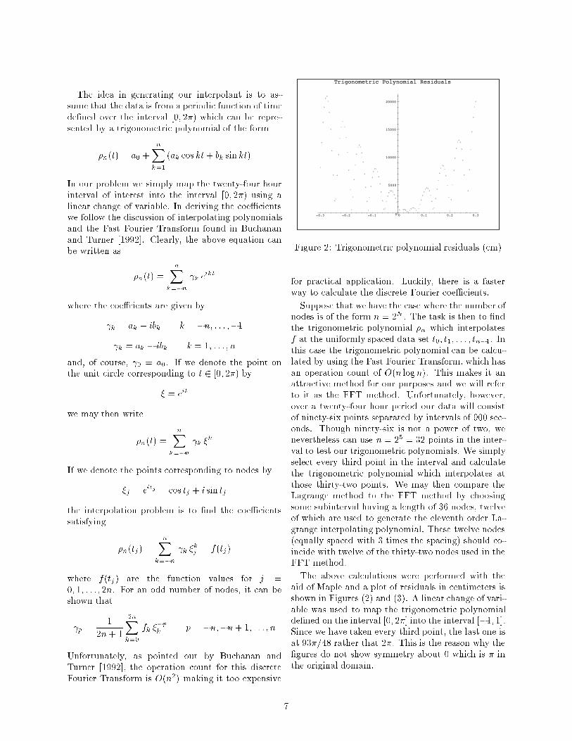
Trigonometric Polynomial Residuals

0

500

1000

1500

2000

2500

0 0.02 0.04 0.06 0.08

Trigonometric Polynomial Residuals

allowed to choose the points on an interval to be inter­polatPd, >YP wo11 ld find th at cPrtain dioicPs of n + 1 poinL:; would yield polynomials which did a bet.Ler job of interpolating than others. As stated, our data poinL:; are evenly spaced Lhroughoul the inLerval of interest, so that will not have the luxury of choosing a prpforrPd sPt of n + 1 points on any intPrval im lPss we are able Lo genera.Le more <la.La. The following dis­cussion closely follows the treatment given by Press eL al [1992]. The Tsheby:;hev polynomial of degree n on [ -1, 1] is defined as

Tn(t) = cos(narccost)

It follows that thP TshPbyslwv polynomials satisfy Lhe three Lenn recurrence relation

T,1+1(t) = 2tTn(t) -Tn_i(t) n = L2, ...

In addition,

and

f1 T,, (l) n(L) = { 1T ,

·'- 1 Jf=t2 1T / '2

k=n=O k=n#O

so that thP TshPhyshPv polynomials arP orthop;onal on Lhe interval [-1, 1] wiLh respect. Lo the weighL func­tion w(t) = 1/Vf=t2. The first few Tshebyshcv polynomials are given by

'Ti)(l) = 1

Ti (t) = t

T2(t) = 2t2 - 1

'(1 (t) = 41 3 - :::t

'/;1 (t) = 814 - 812 + 1

'f';,(1) = l()t~ - '20t3 + 5t

IL can be shown that. Lhe zeros ofT;,(l) on [-1, 1] are given by

_ ... ["U - 1/2)] l j - CO:; n

j=l,2, ... ,n

and that thP TshPhyshPv polynomials satisfy a dis­crele orLhogonaliLy condition [Pre:;s el al, HJ92]

i i- k i=k'.f-0 i=k=O

The powers oft can also be expressed in the Tshcby­shPv polynomial basis.

Any fund.ion f (l) can be a.pproximaLed by a finite linea.r combination of Tshcbyshev polynomials, i.e.

where

. 1 N .

f(t) = 2a.o +I>"'; (t)

'2 /'1 Cli = -Jr ' -1

i=l

J(t)'!; (t) ;:;-----;;; dt .

v 1 - t.~

These coefficients a, can be computed numerically 11sinp; thP Al Pq11ally spacPd data points

tJ = -1 + jD..t, j = 0, 1, · · ·, Af - l

2 D..t= -­

Al - 1

P.p;. vrn thP rnmpositP midpoint rnlP (wP havP to avoid evalua.Ling the inLegran<l a.L the endpoints, lo and tM-1)

where .f (t j +1 ; 2 ) can be approximated by a quadratic or c11 bic polynomial. b'or Pxa.mplP to 11sP c11 bic splinPs to approximate the integrand, we get

where the integrand g(t) is approximated on the in­tPrval [1.i, 1.i+,] by thP c11 hie polynomial

. . 3 ( )2 . . g(t) =a.j(t-tj) +b.i 1-1.i +c1(t-t.1)+d.i

\Ve can also use the midpoint rule on the two left­most panpls and thP two rightmost panpls only. On Lhe resl of Lhe panels we can use Lhe fourLh order Simpson 's ~ rn lP. This will yiPld thP followinp; ap­proximaLion for the coefficienLs:

a,:

8 2 } '· · + :J_(/M-3 + }/IM-2 + 4,qM-1 ,

f{lj)T;(IJ) 9.i= R

If the number of panels left for Simpson's k rule is not P,VP,n, we can take the tr3pe~oidal rnle OVP,f one of Lhe panels (in here we Look Lhe Lhird from last. panel). For example, we show below the formula for an odd number of panels:

a ,: - 4(72 + - (73 + - (74 + - (7·,+ ~t{ 2 8 4 rr · 3· 3· 3· ·

8 5 } ' . · + :J.(/M-4 + J.(/M-3 + .(/M-2 + 4_qM-l ·

To 8va.hrnte f(r) we then llS8 th8 following r8cm­s10n:

d,\' +l = d;v+2 = 0

j = i\', i\' - 1, · · ·, 2, 1

1 f(_r) = do = rd1 - d., + -c-ac·,. • 2 ..

'l'lw bP,n8fit of 'l'sh8bysh8v 8Xpansion is th at th8 maximum dev iaLion on Lhe int.er val is minimi11ed. Thus it will not suffer from the disadvantage of higher ordP,r polynomi a.ls, th at is the P,rror h8rP, do8sn 't grow rapidly near Lhe en<lpoint.s oft.he interval. Therefore W8 elimin3te the n88d for ''walking'' int8rpolator.

Conclusions

This has been a. preliminary sLudy of various in­terpolation methods for GPS ephemeris data. The 3 Jtern at8 long-arc met hods of int8rpolation we h av8 tried so far yield much greater than 1 cm error when compar8d to the short-3rc 8l8VP,nth ord8r Lagrange polynomial. However, more work should be done be­fore completely ruling out these alternate methods.

Our study docs indicate that the use of diffcr­P,nC8 t3 bl8s should h8 mor8 effici8nt th an th8 direct m ethod currently used to construct and evaluate the Lagrnng8 polynomials.

Acknowledge1nent

This research was supporLed in pal'L by t.he Na.val Postgraduate School R.cscarch Program. The authors gra.Lefully acknowledge t.he parLial supporL of ~ISE 'Vest Coast Division.

References

10

Ahlberg, J. H., ~ilson, E. I\., and 'Valsh, J. L., 1967, 'lhF thmry of Splines and '/'heir Applirations, (l\8w York: Springer Verlag)

Driggs, \V.L. and Ilenson, V. E., 199;), Tht DI'T. Ari Owner '.s Afcmvol for the Di.scrctc Fo-uricr Transform. (Philad8lphia: Sl;\M)

Brigham, E. 0., 1988, The Fast Fourier Transform. artd Its Applualioris, (I\ ew Jersey: Pren Lice Ilall)

Hudrnnan, .J.L. and '1'11rn8r, P.K .. , HHJ2, i\'11meriral Afr/hods arid Arialybib, (New York: l\foC raw-Ilill, Inc.)

de Boor, C., 1978, il I'rnctical Guide to Spline.s, vol. 27 of Applied Mathematical S'rienr:es, (l\8w York: Springer-Verlag)

Goert~8l. G., Hl60, FomiN S8ries, Afatlwmatiral Methods for Diqital Cornptders, (New York: 'Vilcy)

Malys, S., an<l OrLi:-1, ~VI. J., 1989, Geodetic absolut.e positioning with differenced G PS ca.rricr beat phase dat3, Proc88dings of the 5111 International Sympo­sium on Satellite Positioning, 13-17 March 1989, Las Crnc8s, I\ M.

Press, \V. H., Flannery, B. P., Teukolsky, S. A., and VettP,rling, \V. T., HHJ2, i\'111nairal Heripes in FOH­TRi lN, The ilrt of Scientific Compvtinq, 2nd Edi­tion, (l\8w York: Cambridg8 Univ8rsity Pr8ss)

R.cmondi, B. \V., 1989, E.rteridinq the National Geodetir S'urr;ey Standard GPS' Orbit Formats, NOAA Technical Ilepol'L NOS 1:1:1 NGS 'rn, (K.ockville, \·11): LS Dep3rtm8nt of Commerc8, NOAA)

K,emondi, H. W., HH_ll, i\'GS' Second Generation ASCII artd Buwry Orbit Formals artd Asbocialtd In­terpolation Studies, ( l{ockvill8, i'vl D: US Dep3rtm8nt of Commerce, NOAA)

Smith, I{. and Curtis, V., 198:), lnt8rpobtion Study, Na.val Surface 'Vea.pons CenLer Dahlgren LaboraLory Memorandum.

"'atkins, M., 1995, Private communication.