Interpolation

Basic interpolation problem: for given data

(ti, yi), i = 1, . . . , m,

with t1 < t2 < . . . < tm, determine function

f :R → R such that

f(ti) = yi, i = 1, . . . , m

f is interpolating function, or interpolant, for

given data

Additional data might be prescribed, such as

slope of interpolant at given points

Additional constraints might be imposed, such

as smoothness, monotonicity, or convexity of

interpolant

f could be function of more than one variable,

but we will consider only one-dimensional case

2

Purposes for Interpolation

• Plotting smooth curve through discrete data

points

• Reading between lines of table

• Differentiating or integrating tabular data

• Quick and easy evaluation of mathematical

function

• Replacing complicated function by simple

one

3

Interpolation vs Approximation

By definition, interpolant function fits given

data points exactly

Interpolation inappropriate if data points sub-

ject to significant errors

Usually preferable to smooth noisy data, for

example by least squares approximation

Approximation also appropriate for special func-

tion libraries

4

Issues in Interpolation

Arbitrarily many functions interpolate given data

points

• What form should function have?

• How should function behave between data

points?

• Should function inherit properties of data,

such as monotonicity, convexity, or period-

icity?

• Are parameters that define interpolating

function meaningful?

• If function and data are plotted, should re-

sults be visually pleasing?

5

Choosing Interpolant

Choice of function for interpolation based on

• How easy function is to work with

− determining its parameters

− evaluating function

− differentiating or integrating function

• How well properties of function match prop-

erties of data to be fit (smoothness, mono-

tonicity, convexity, periodicity, etc.)

6

Functions for Interpolation

Families of functions commonly used for inter-

polation include

• Polynomials

• Piecewise polynomials

• Trigonometric functions

• Exponential functions

• Rational functions

We will focus on interpolation by polynomials

and piecewise polynomials for now

Will consider trigonometric interpolation (DFT)

later

7

Basis Functions

Family of functions for interpolating given data

points is spanned by set of basis functions φ1(t),

. . . , φn(t)

Interpolating function f chosen as linear com-

bination of basis functions,

f(t) =n∑

j=1

xjφj(t)

Requiring f to interpolate data (ti, yi) means

f(ti) =n∑

j=1

xjφj(ti) = yi, i = 1, . . . , m,

which is system of linear equations

Ax = y

for n-vector x of parameters xj, where entries

of m× n matrix A are given by aij = φj(ti)

8

Existence, Uniqueness, and Conditioning

Existence and uniqueness of interpolant de-

pend on number of data points m and number

of basis functions n

If m > n, interpolant usually doesn’t exist

If m < n, interpolant not unique

If m = n, then basis matrix A nonsingular,

provided data points ti distinct, so data can

be fit exactly

Sensitivity of parameters x to perturbations in

data depends on cond(A), which depends in

turn on choice of basis functions

9

Polynomial Interpolation

Simplest and most common type of interpola-

tion uses polynomials

Unique polynomial of degree at most n − 1

passes through n data points (ti, yi), i = 1, . . . , n,

where ti are distinct

There are many ways to represent or compute

polynomial, but in theory all must give same

result

10

Monomial Basis

Monomial basis functions,

φj(t) = tj−1, j = 1, . . . , n,

give interpolating polynomial of form

pn−1(t) = x1 + x2t + · · ·+ xntn−1,

with coefficients x given by n×n linear system

Ax =

1 t1 · · · tn−1

11 t2 · · · tn−1

2... ... . . . ...

1 tn · · · tn−1n

x1

x2...

xn

=

y1

y2...

yn

= y

Matrix of this form called Vandermonde matrix

11

Example: Monomial Basis

Find polynomial of degree two interpolating

three data points (−2,−27), (0,−1), (1,0)

Using monomial basis, linear system is

Ax =

1 t1 t211 t2 t221 t3 t23

x1

x2

x3

=

y1

y2

y3

= y

For these particular data, system is1 −2 4

1 0 0

1 1 1

x1

x2

x3

=

−27

−1

0

,

whose solution is x = [−1 5 −4 ]T , so in-

terpolating polynomial is

p2(t) = −1 + 5t− 4t2

12

Monomial Basis, continued

Solving system Ax = y using standard linear

equation solver to determine coefficients x of

interpolating polynomial requires O(n3) work

For monomial basis, matrix A often ill-conditioned,

especially for high-degree polynomials

0.0 0.5 1.00.0

0.5

1.0

...................

...................

...................

...................

...................

...................

...................

...................

...................

...................

...................

...................

...................

...................

...................

...................

...................

...................

...................

...................

...................

...................

...................

.......................................................................................................................................................................................................................................................................................................................................................................................................................................................................................................................................................................................................................................................................................................................................................................................................................................................................................................................................................

....................................................................................

....................................................................................

....................................................................................

....................................................................................

....................................................................................

....................................................................................

....................................................................................

....................................................................................

....................................................................................

....................................................................................

....................................................................................

....................................................................................

...

........................................................................................................................................................................................................................................................................

.................................................................................................................

..........................................................................................

...............................................................................

........................................................................

....................................................................................................................................................................................................................................................................................................................................................................................................................................

................................................................................................................................................................................................................................................................................................................................................................................................................

............................................................................................................

................................................................................

.................................................................................................................................................................................................................................................................................................................................................................................................................................................................................................

.............................................................................................................................................................................................................................................................................................................................................................................................................................................................................................................

.................................................................................................

.........................................................................................................................................................................................................................................................................................................................................................................................................................................................................................................................

.............................................................................................................................................................................................................................................................................................................................................................................................................................................................................................................................................................................

........................................................................................

........................................................................................................................................................................................................................................................................................................................................................................................................................................................................................

..............................................................................................................................................................................................................................................................................................................................................................................................................................................................................................................................................................................................................................

................................................................................

................................................................................................................................................................................................................................................................................................................................................................................................................................................................

..................................................................................................................................................................................................................................................................................................................................................................................................................................................................................................................................................................................................................................................................

............................................................................................................................................................................................................................................................................................................................................................................................................................................................................................................................

...............................................................................................................................................................................................................................................................................................................................................................................................................................................................................................................................................................................................................................................................................................

...........................................................................................................................................................................................................................................................................................................................................................................................................................................................................................................1

t

t2

t3

13

Monomial Basis, continued

Ill-conditioning does not prevent fitting data

points well, since residual for linear system so-

lution will be small

But it does mean that values of coefficients

may be poorly determined

Both conditioning of linear system and amount

of computational work required to solve it can

be improved by using different basis

Change of basis still gives same interpolating

polynomial for given data, but representation

of polynomial will be different

14

Monomial Basis, continued

Conditioning with monomial basis can be im-

proved by shifting and scaling independent vari-

able t:

φj(t) =(

t− c

d

)j−1,

where, c = (t1 + tn)/2 is midpoint and d =

(tn − t1)/2 is half of range of data

New independent variable lies in interval [−1,1],

which also helps avoid overflow or harmful un-

derflow

Even with optimal shifting and scaling, mono-

mial basis usually still poorly conditioned, and

we seek better alternatives

15

Evaluating Polynomials

When represented in monomial basis, polyno-

mial

pn−1(t) = x1 + x2t + · · ·+ xntn−1

can be evaluated efficiently using Horner’s nested

evaluation scheme:

pn−1(t) = x1+t(x2+t(x3+t(· · · (xn−1+txn) · · ·))),which requires only n additions and n multipli-

cations

For example,

1−4t+5t2−2t3+3t4 = 1+t(−4+t(5+t(−2+3t)))

Other manipulations of interpolating polyno-

mial, such as differentiation or integration, are

also relatively easy with monomial basis repre-

sentation16

Lagrange Interpolation

For given set of data points (ti, yi), i = 1, . . . , n,

Lagrange basis functions given by

`j(t) =n∏

k=1,k 6=j

(t− tk) /n∏

k=1,k 6=j

(tj − tk),

j = 1, . . . , n

For Lagrange basis,

`j(ti) =

{1 if i = j0 if i 6= j

, i, j = 1, . . . , n

so matrix of linear system Ax = y is identity

Thus, Lagrange polynomial interpolating data

points (ti, yi) given by

pn−1(t) = y1`1(t) + y2`2(t) + · · ·+ yn`n(t)

17

Lagrange Basis Functions

0.0 0.5 1.0

0.0

0.5

1.0 ...........................................................................................................................................................................................................................................................................................................................................................................................................................................................................................................................................................................................................................................................................................................................................................................................................................................................................................................................................................................................................................................................................................................................................................................................................................................................................................................................................................................................................................................................................................................................................................................................................................

......................................................

.......................................................................................................................................................................................................................................................

.........................................................................................................................................................................................................................................................

..........................................................................................................................................................................................................................................................................................................................................................................................................................

.......................................... ..................... ..................... ..................... ..................... ..................... ..................... ..................... ..................... .....................

..........................................

...................................................................................................................................................

..................... ..................... ...............................................................

................................................................................................................................... ............................... ............................... ............................... ............................... ............................... ............................... ............................... ............................... ............................... ............................... ............................... ...............................

............................................................................................................................

`1

`2`3

`4

`5

Lagrange interpolant is easy to determine but

more expensive to evaluate for given argument,

compared with monomial basis representation

Lagrangian form is also more difficult to dif-

ferentiate, integrate, etc.

18

Example: Lagrange Interpolation

Use Lagrange interpolation to find interpolat-

ing polynomial for three data points (−2,−27),

(0,−1), (1,0)

Lagrange polynomial of degree two interpolat-

ing three points (t1, y1), (t2, y2), (t3, y3) is

p2(t) = y1(t− t2)(t− t3)

(t1 − t2)(t1 − t3)+y2

(t− t1)(t− t3)

(t2 − t1)(t2 − t3)

+y3(t− t1)(t− t2)

(t3 − t1)(t3 − t2)

For these particular data, this becomes

p2(t) = −27t(t− 1)

(−2)(−2− 1)+(−1)

(t + 2)(t− 1)

(2)(−1)

19

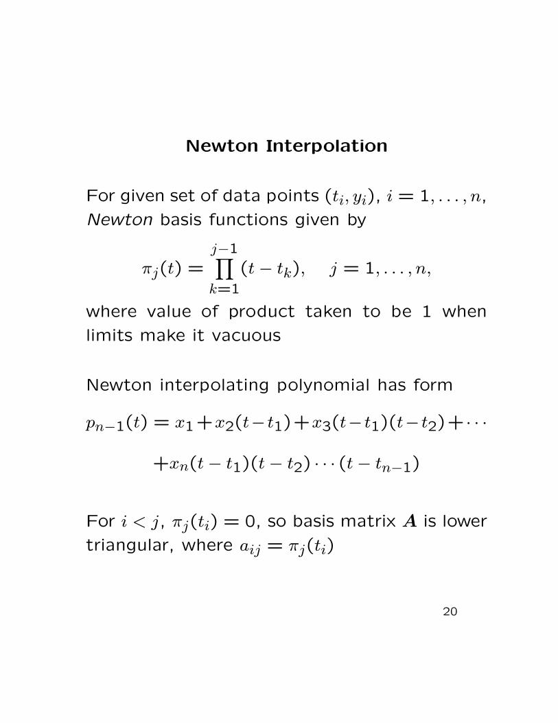
Newton Interpolation

For given set of data points (ti, yi), i = 1, . . . , n,

Newton basis functions given by

πj(t) =j−1∏k=1

(t− tk), j = 1, . . . , n,

where value of product taken to be 1 when

limits make it vacuous

Newton interpolating polynomial has form

pn−1(t) = x1+x2(t− t1)+x3(t− t1)(t− t2)+ · · ·

+xn(t− t1)(t− t2) · · · (t− tn−1)

For i < j, πj(ti) = 0, so basis matrix A is lower

triangular, where aij = πj(ti)

20

Newton Interpolation, continued

Hence, solution x to system Ax = y can be

computed by forward-substitution in O(n2) arith-

metic operations

Moreover, resulting interpolant can be eval-

uated efficiently for any argument by nested

evaluation scheme similar to Horner’s method

Newton interpolation has better balance be-

tween cost of computing interpolant and cost

of evaluating it

0.0 0.5 1.0 1.5 2.0

0.0

1.0

2.0

3.0

........................................................................................................................................................................................................................................................................................................................................................................................................................................................................................................................................................................................................................................................................................................................................................................................................................................................................................................................................

................................................................................................

................................................................................................

................................................................................................

................................................................................................

................................................................................................

..............................................................................

..................................................................................................................................................................................................................

.................................................................

.......................................................

............................................

............................................

............................................

............................................

..........................................

..................... ..................... ..................... ..................... ..................... ..................... ..................... ..................... ..................... ..................... ..................... ..................... ..................... ..................... .....................

..................... ..................... .

.........................................

...................................................................................................................................................

............................... ............................... ............................... ............................... ............................... ............................... ............................... ............................... ............................... ............................... ............................... ............................... ..............................................................

....................................................................

π1π2 π3 π4 π5

21

Example: Newton Interpolation

Use Newton interpolation to find interpolat-

ing polynomial for three data points (−2,−27),

(0,−1), (1,0)

Using Newton basis, linear system is1 0 0

1 t2 − t1 0

1 t3 − t1 (t3 − t1)(t3 − t2)

x1

x2

x3

=

y1

y2

y3

For these particular data, system is1 0 0

1 2 0

1 3 3

x1

x2

x3

=

−27

−1

0

,

whose solution by forward substitution is x =

[−27 13 −4 ]T , so interpolating polynomial

is

p(t) = −27 + 13(t + 2)− 4(t + 2)t

22

Newton Interpolation, continued

If pj(t) is polynomial of degree j−1 interpolat-

ing j given points, then for any constant xj+1,

pj+1(t) = pj(t) + xj+1πj+1(t)

is polynomial of degree j that also interpolates

same j points

Free parameter xj+1 can then be chosen so

that pj+1(t) interpolates yj+1. Specifically,

xj+1 =yj+1 − pj(tj+1)

πj+1(tj+1)

Newton interpolation begins with constant poly-

nomial p1(t) = y1 interpolating first data point

and then successively incorporates remaining

data points into interpolant

23

Divided Differences

Given data points (ti, yi), i = 1, . . . , n, divided

differences, denoted by f [ ], defined recursively

by

f [t1, t2, . . . , tk] =f [t2, t3, . . . , tk]− f [t1, t2, . . . , tk−1]

tk − t1,

where recursion begins with f [tk] = yk, k =

1, . . . , n

Coefficient of jth basis function in Newton in-

terpolant given by

xj = f [t1, t2, . . . , tj]

Recursion requires O(n2) arithmetic operations

to compute coefficients of Newton interpolant,

but is less prone to overflow or underflow than

direct formation of triangular Newton basis ma-

trix

24

Orthogonal Polynomials

Inner product can be defined on space of poly-

nomials on interval [a, b] by taking

(p, q) =∫ b

ap(t)q(t)w(t)dt,

where w(t) is nonnegative weight function

Two polynomials p and q are orthogonal if

(p, q) = 0

Set of polynomials {pi} is orthonormal if

(pi, pj) =

{1 if i = j0 otherwise

Given set of polynomials, Gram-Schmidt or-

thogonalization can be used to generate or-

thonormal set spanning same space

25

Orthogonal Polynomials, continued

For example, with inner product given by weight

function w(t) ≡ 1 on interval [−1,1], apply-

ing Gram-Schmidt process to set of monomials

1, t, t2, t3, . . . yields Legendre polynomials

1, t, (3t2 − 1)/2, (5t3 − 3t)/2,

(35t4−30t2+3)/8, (63t5−70t3+15t)/8, . . . ,

first n of which form an orthogonal basis for

space of polynomials of degree at most n− 1

Other choices of weight functions and inter-

vals yield other orthogonal polynomials, such

as Chebyshev, Jacobi, Laguerre, and Hermite

26

Orthogonal Polynomials, continued

Orthogonal polynomials have many useful prop-

erties

They satisfy three-term recurrence relation of

form

pk+1(t) = (αkt + βk)pk(t)− γkpk−1(t),

which makes them very efficient to generate

and evaluate

Orthogonality makes them very natural for least

squares approximation, and they are also useful

for generating Gaussian quadrature rules

27

Chebyshev Polynomials

kth Chebyshev polynomial of first kind defined

on interval [−1,1] by

Tk(t) = cos(k arccos(t))

are orthogonal with respect to weight function

(1− t2)−1/2

First few Chebyshev polynomials given by

1, t, 2t2 − 1, 4t3 − 3t, 8t4 − 8t2 + 1,

16t5 − 20t3 + 5t, . . . .

Equi-oscillation property: successive extrema

of Tk are equal in magnitude and alternate

in sign, which distributes error uniformly when

approximating arbitrary continuous function

28

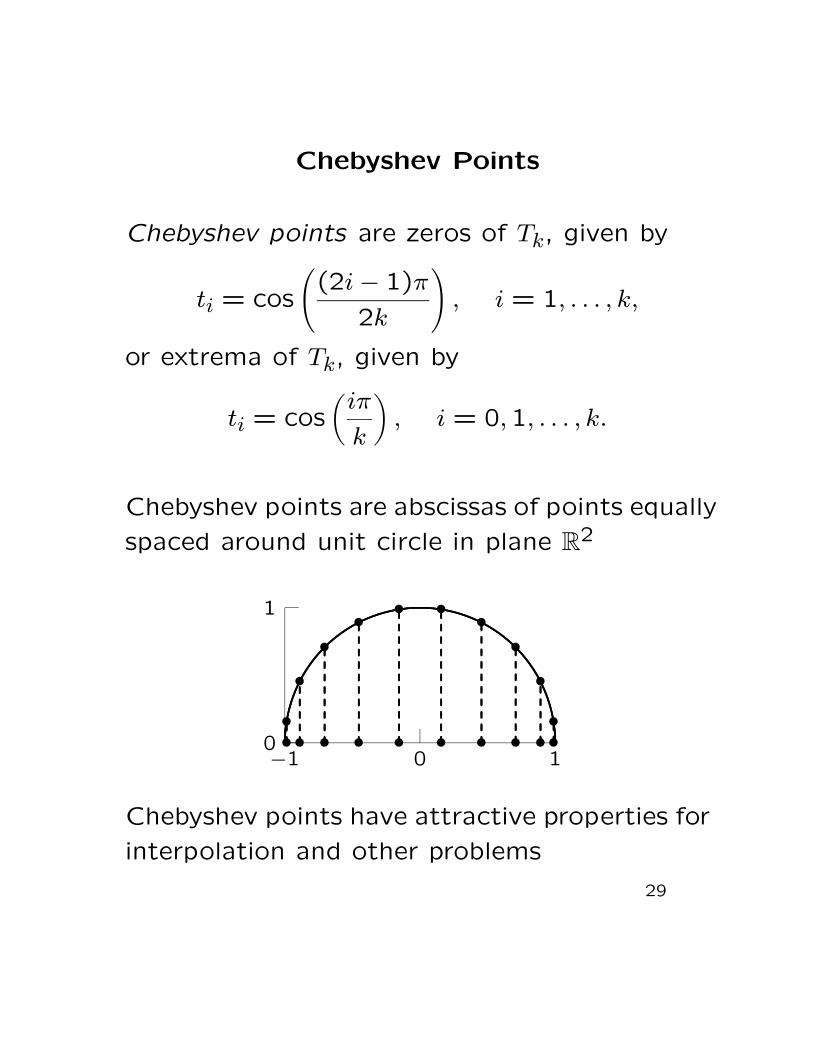
Chebyshev Points

Chebyshev points are zeros of Tk, given by

ti = cos

((2i− 1)π

2k

), i = 1, . . . , k,

or extrema of Tk, given by

ti = cos(

iπ

k

), i = 0,1, . . . , k.

Chebyshev points are abscissas of points equally

spaced around unit circle in plane R2

−1 0 10

1

...................

...................

.........................................................................................................................................................................

..........................................................

..........................................................................................

............................................................................................................................................................................................................................................................................................................................................................................................................................................................................................................................................................................................................

.............

.............

.............

.............

.............

.............

.............

.............

.............

.............

.............

.............

.............

.............

.............

.............

.............

.............

.............

.............

.............

.............

.............

.............

.............

.............

.............

.............

.............

.............

.............

.............

.............

.............

.............

.............

.............

.............

.............

.............

.............

.............

.............

.............

.............

.............

.............

.............

.............

.............

.............

.............

.............

.............

.............

.............

.............

.............

.............

.............

.............

.............

.............

.............

.............•••

• • • ••••

•• • • • • • • ••

Chebyshev points have attractive properties for

interpolation and other problems

29

Interpolating Continuous Functions

If data points are discrete sample of continu-

ous function, how well does interpolant approx-

imate that function between sample points?

If f is smooth function, and pn−1 is polynomial

of degree at most n − 1 interpolating f at n

points t1, . . . , tn, then

f(t)−pn−1(t) =f(n)(θ)

n!(t−t1)(t−t2) · · · (t−tn),

where θ is some (unknown) point in interval

[t1, tn]

Since point θ unknown, result not particularly

useful unless bound on appropriate derivative

of f is known

30

Interpolating Continuous Functions, cont.

If |f(n)(t)| ≤ M for all t ∈ [t1, tn], and h =

max{ti+1 − ti : i = 1, . . . , n− 1}, then

maxt∈[t1,tn]

|f(t)− pn−1(t)| ≤Mhn

4n

Error diminishes with increasing n and decreas-

ing h, but only if |f(n)(t)| does not grow too

rapidly with n

31

High-Degree Polynomial Interpolation

Interpolating polynomials of high degree are

expensive to determine and evaluate

In some bases, coefficients of polynomial may

be poorly determined due to ill-conditioning of

linear system to be solved

High-degree polynomial necessarily has lots of

“wiggles,” which may bear no relation to data

to be fit

Polynomial goes through required data points,

but it may oscillate wildly between data points

32

Nonconvergence

Polynomial interpolating continuous function

at equally spaced points may not converge to

function as number of data points and polyno-

mial degree increases

Example: Polynomial interpolants of Runge’s

function at equally spaced points

−1.0 −0.5 0.0 0.5 1.00.0

0.5

1.0

1.5

2.0

...................................................................................................................................................................................................................................................................

........................................................................................................................................................................................................................................................................................................................................................................................................................................................................................................................................................................................................................................................................................................................................................................................................................................................................................................................................................................................

................................................................................

........................................

........................................................................................................................................................................................................................................................................................................................................

...........................................................................................................................................................................................................................................................

....................................................

.....................................................................................................................................................................

...................................................................................................................................................................................................................................

f(t) = 1/(1 + 25t2)...........................................................................................

p5(t).................................................

p10(t)...................

33

Placement of Interpolation Points

Equally spaced interpolation points often yield

unsatisfactory results near ends of interval

If points are bunched near ends of interval,

more satisfactory results likely to be obtained

with polynomial interpolation

For example, use of Chebyshev points distributes

error evenly and yields convergence throughout

interval for any sufficiently smooth function

34

Placement of Points, continued

Example: Polynomial interpolants of Runge’s

function at Chebyshev points

−1.0 −0.5 0.0 0.5 1.00.0

0.5

1.0

1.5

2.0

...................................................................................................................................................................................................................................................................

........................................................................................................................................................................................................................................................................................................................................................................................................................................................................................................................................................................................................................................................................................................................................................................................................................................................................................................................................................................................

......................................................

..........................................................

....................................................................................................................................................................................................................................................................................................................................................

.....................................

..........................................................................................................................................................................

..........

f(t) = 1/(1 + 25t2)...........................................................................................

p5(t).................................................

p10(t)...................

35

Taylor Polynomial

Another useful form of polynomial interpola-

tion for smooth function f is polynomial given

by truncated Taylor series

pn(t) = f(a)+ f ′(a)(t− a)+f ′′(a)

2(t− a)2 + · · ·

+f(n)(a)

n!(t− a)n

Polynomial interpolates f in that values of pn

and its first n derivatives match those of f and

its first n derivatives evaluated at t = a, so

pn(t) is good approximation to f(t) for t near

a

We have already seen examples in Newton’s

method for nonlinear equations and optimiza-

tion

36

Piecewise Polynomial Interpolation

Fitting single polynomial to large number of

data points is likely to yield unsatisfactory os-

cillating behavior in interpolant

Piecewise polynomials provide alternative to

practical and theoretical difficulties with high-

degree polynomial interpolation

Main advantage of piecewise polynomial inter-

polation is that large number of data points

can be fit with low-degree polynomials

In piecewise interpolation of given data points

(ti, yi), different function is used in each subin-

terval [ti, ti+1]

Abscissas ti are called knots or breakpoints, at

which interpolant changes from one function

to another37

Piecewise Interpolation, continued

Simplest example is piecewise linear interpola-

tion, in which successive pairs of data points

are connected by straight lines

Although piecewise interpolation eliminates ex-

cessive oscillation and nonconvergence, it ap-

pears to sacrifice smoothness of interpolating

function

We have many degrees of freedom in choos-

ing piecewise polynomial interpolant, however,

which can be exploited to obtain smooth inter-

polating function despite its piecewise nature

38

Hermite Interpolation

In Hermite interpolation, derivatives as well as

values of interpolating function are specified at

data points

Specifying derivative values adds more equa-

tions to linear system that determines param-

eters of interpolating function

To have unique solution, number of equations

must equal number of parameters to be deter-

mined

Piecewise cubic polynomials are typical choice

Hermite interpolation, providing flexibility, sim-

plicity and efficiency

39

Hermite Cubic Interpolation

Hermite cubic interpolant is piecewise cubic

polynomial interpolant with continuous first deriva-

tive

Piecewise cubic polynomial with n knots has

4(n− 1) parameters to be determined

Requiring that it interpolate given data gives

2(n− 1) equations

Requiring that it have one continuous deriva-

tive gives n − 2 additional equations, or total

of 3n− 4, which still leaves n free parameters

Thus, Hermite cubic interpolant is not unique,

and remaining free parameters can be chosen

so that result satisfies additional constraints

40

Cubic Spline Interpolation

Spline is piecewise polynomial of degree k that

is k − 1 times continuously differentiable

For example, linear spline is of degree 1 and has

0 continuous derivatives, i.e., it is continuous,

but not smooth, and could be described as

“broken line”

Cubic spline is piecewise cubic polynomial that

is twice continuously differentiable

As with Hermite cubic, interpolating given data

and requiring one continuous derivative imposes

3n− 4 constraints on cubic spline

Requiring continuous second derivative imposes

n− 2 additional constraints, leaving 2 remain-

ing free parameters

41

Cubic Splines, continued

Final two parameters can be fixed in various

ways:

• Specifying first derivative at endpoints t1and tn

• Forcing second derivative to be zero at

endpoints, which gives natural spline

• Enforcing “not-a-knot” condition, forcing

two consecutive cubic pieces to be same

• Forcing first derivatives, as well as second

derivatives, to match at endpoints t1 and

tn (if spline is to be periodic)

42

Example: Cubic Spline Interpolation

Determine natural cubic spline interpolating three

data points (ti, yi), i = 1,2,3

Required interpolant is piecewise cubic func-

tion defined by separate cubic polynomials in

each of two intervals [t1, t2] and [t2, t3]

Denote these two polynomials by

p1(t) = α1 + α2t + α3t2 + α4t3,

p2(t) = β1 + β2t + β3t2 + β4t3

Eight parameters are to be determined, so we

need eight equations

Requiring first cubic to interpolate data at end

points of first interval gives two equations

α1 + α2t1 + α3t21 + α4t31 = y1,

43

Example Continued

α1 + α2t2 + α3t22 + α4t32 = y2

Requiring second cubic to interpolate data at

end points of second interval gives two equa-

tions

β1 + β2t2 + β3t22 + β4t32 = y2,

β1 + β2t3 + β3t23 + β4t33 = y3

Requiring first derivative of interpolant to be

continuous at t2 gives equation

α2 + 2α3t2 + 3α4t22 = β2 + 2β3t2 + 3β4t22

44

Example Continued

Requiring second derivative of interpolant func-

tion to be continuous at t2 gives equation

2α3 + 6α4t2 = 2β3 + 6β4t2

Finally, by definition natural spline has second

derivative equal to zero at endpoints, which

gives two equations

2α3 + 6α4t1 = 0,

2β3 + 6β4t3 = 0

When particular data values are substituted for

ti and yi, system of eight linear equations can

be solved for eight unknown parameters αi and

βi

45

Hermite Cubic vs Spline Interpolation

Choice between Hermite cubic and spline in-

terpolation depends on data to be fit and on

purpose for doing interpolation

If smoothness is of paramount importance, then

spline interpolation may be most appropriate

But Hermite cubic interpolant may have more

pleasing visual appearance and allows flexibility

to preserve monotonicity if original data are

monotonic

In any case, it is advisable to plot interpolant

and data to help assess how well interpolating

function captures behavior of original data

46

Hermite Cubic vs Spline Interpolation

0 2 4 6 8 100

2

4

6

8•

• •

• • • • •

.......................................................................................................................................................................................................................................................................................................................................................................................................................................................................................................................................................................................................................................................................................................................................................................................................................................................................................................................................................

monotoneHermite cubic

0 2 4 6 8 100

2

4

6

8•

• •

• • • • •

.........................................................................................................................................................................................................................................................................................................................................................................................................................................................................................................................................................................................................................................................

.......................................................................................................................................................................................................................................................................................................................................................

cubic spline

47

B-splines

B-splines form basis for family of spline func-

tions of given degree

B-splines can be defined in various ways, in-

cluding recursion, convolution, and divided dif-

ferences. Here we will define them recursively

Although in practice we use only finite set of

knots t1, . . . , tn, for notational convenience we

will assume infinite set of knots

· · · < t−2 < t−1 < t0 < t1 < t2 < · · ·Additional knots can be taken as arbitrarily de-

fined points outside interval [t1, tn]

We will also use linear functions

vki (t) = (t− ti)/(ti+k − ti)

48

B-splines, continued

To start recursion, define B-splines of degree

0 by

B0i (t) =

{1 if ti ≤ t < ti+10 otherwise

,

and then for k > 0 define B-splines of degree

k by

Bki (t) = vk

i (t)Bk−1i (t) + (1− vk

i+1(t))Bk−1i+1(t)

Since B0i is piecewise constant and vk

i is linear,

B1i is piecewise linear

Similarly, B2i is in turn piecewise quadratic, and

in general, Bki is piecewise polynomial of degree

k

49

B-splines

0.0

0.5

1.0 ..............................................................................................................................................................................................................................................................................................................................................................................................................ti ti+1 ti+2 ti+3 ti+4

B0i

0.0

0.5

1.0

....................................................................................................................................................................................................................................................................................................................................................................................................................................................................................................................................................................................

ti ti+1 ti+2 ti+3 ti+4

B1i

0.0

0.5

1.0

.................................................................................................................................

............................................................................................................................................................................................................................................................................................................................................................................................................................................................................................................................................................................

ti ti+1 ti+2 ti+3 ti+4

B2i

0.0

0.5

1.0

......................................................................................................................................................................................................................

.............................................................................................................................................

......................................................................................................................................................................................................................................................................................................................................................................................................................................................................................................................

ti ti+1 ti+2 ti+3 ti+4

B3i

50

B-splines, continued

Important properties of B-spline functions Bki :

1. For t < ti or t > ti+k+1, Bki (t) = 0

2. For ti < t < ti+k+1, Bki (t) > 0

3. For all t,∑∞

i=−∞Bki (t) = 1

4. For k ≥ 1, Bki has k − 1 continuous

derivatives

5. Set of functions {Bk1−k, . . . , Bk

n−1} is linearly

independent on interval [t1, tn] and spans

space of all splines of degree k having knots

ti

51

B-splines, continued

Properties 1 and 2 together say that B-spline

functions have local support

Property 3 gives normalization

Property 4 says that they are indeed splines

Property 5 says that for given k these functions

form basis for set of all splines of degree k

52

B-splines, continued

If we use B-spline basis, linear system to be

solved for spline coefficients will be nonsingular

and banded

Use of B-spline basis yields efficient and sta-

ble methods for determining and evaluating

spline interpolants, and many library routines

for spline interpolation are based on this ap-

proach

B-splines are also useful in many other con-

texts, such as numerical solution of differential

equations, as we will see later

53