Interpolation And Visualization For Advected Scalar Fields

Shyh-Kuang Ueng∗ Sheng-Chuan Wang†

Department of Computer Science

National Taiwan Ocean University

No. 2, Pei-Ning Road, Keelung, Taiwan 202

ABSTRACT

Doppler radars are useful facilities for weather forecasting. Thedata sampled by using Doppler radars are used to measure the dis-tributions and densities of rain drops, snow crystals, hail stones, oreven insects in the atmosphere. In this paper, we propose to buildup a graphics-based software system for visualizing Doppler radardata. In the system, the reflectivity data gathered by using Dopplerradars are post-processed to generate virtual cloud images whichreveal the densities of precipitation in the air. An optical flow basedmethod is adopted to compute the velocities of clouds, advected bywinds. Therefore, the movement of clouds is depicted. The cloudvelocities are also used to interpolate reflectivities for arbitrary timesteps. Therefore, the reflectivities at any time can be produced. Oursystem composes of three stages. At the first stage, the raw radardata are re-sampled and filtered to create a multiple resolution datastructure, based on a pyramid structure. At the second stage, a nu-meric method is employed to compute cloud velocities in the airand to interpolate radar reflectivity data at given time steps. Theradar reflectivity data and cloud velocities are displayed at the laststage. The reflectivities are rendered by using splatting methodsto produce semi-transparent cloud images. Two kinds of media arecreated for analyzing the reflectivity data. The first kind media con-sists of a group of still images of clouds which displays the distribu-tion and density of water in the air. The second type media is a shortanimation of cloud images to show the formation and movement ofthe clouds. To show the advection of clouds, the cloud velocitiesare displayed by using two dimensional images. In these images,the velocities are represented by arrows and superimposed on cloudimages.

To enhance image quality, gradients and diffusion of the radardata are computed and used in the rendering process. Therefore thecloud structures are better portrayed. In order to achieve interactivevisualization, our system is also comprised with a view-dependentvisualization module. The radar data at far distance are renderedin lower resolutions, while the data closer to the eye position isrendered in details.

CR Categories: I.3.3 [Computer Graphics]: Picture/ImageGeneration—Display Algorithms;

Keywords: Doppler radar, volume rendering, optical flow, level ofdetails, vector field visualization

1 INTRODUCTION

A Doppler radar is used for the measurement of rainfall intensity. Itsends out microwave pulses toward the air. When the waves hit ob-jects, small fractions of the waves are scattered back to the antenna

∗e-mail: skueng@mail.ntou.edu.tw†e-mail: b88048@cyber.cs.ntou.edu.tw

of the radar. The reflectivities are transformed into scalar values torepresent the density of precipitation in the air. The radar can rotate360 degrees about the vertical axis. For each degree of angle, theradar sends out pulses to sense the particles in the air. The densitiesof particles are measured at equidistant points along each ray. Af-ter completing a circular scanning, the radar raises up its elevationangle by several degrees and performs the circular scanning again[1, 7, 6]. The sample points of the radar are located on multiple lay-ers of concentric conical surfaces. The data set contain millions ofpoints and is too large to be analyzed by hand. Therefore computerprograms are employed for post-processing these data.

1.1 Previous Work

Many computer algorithms have been designed for post-processingmeteorological data. In [15], a multiresolution method is presentedfor visualizing weather radar data. In their method, a hierarchicalstructure of tetrahedral meshes is created upon the data. Lower rep-resentations of the data are used for displaying areas of small varia-tion while higher resolution representations are rendered for explor-ing important features. Clouds are displayed by compositing multi-ple transparent iso-surfaces. Djurcilov and Pang developed anotheriso-surface based visualization technique for processing radar data.In their method, the radar data are filtered at first to smooth thedata and to recover missing values. Then iso-surfaces are created toshow the distribution of precipitation in the air [9]. These two iso-surface visualization methods suffer from missing the fine detailsof the cloud structure. The appearance of clouds generated by theirsystems does not look natural when compared with satellite cloudimages. Treinish presents a method for visualizing scattered mete-orological data [36]. In his method, a mesh is imposed upon thedomain at first. Then the data are re-sampled at the mesh verticessuch that traditional visualization softwares and hardwares can beutilized for displaying the data. His system has been successfullyused for showing the rainfall distribution in Peru. Jang et al. designa LoD visualization system for radar data. At first the data set issplit to create a hierarchical data structure, the volume tree. Thensplatting volume rendering is used to render the data to reveal radarreflectivities. They also used view-dependent strategies to improvethe performance of their rendering process. However, lacking of agood lighting method and any cloud structure enhancement skill,the images generated by these two systems do not reveal the detailsof the clouds.

A visualization system called D3D is proposed in [27]. The sys-tem was developed based on its precedent system, Vis5D, and newfunctionalities are added such that both 3D and 2D meteorologi-cal data can be processed. The authors suggest that 2D graphicalfigures may be superior to 3D volume rendering images in certainapplications. However, 3D volume visualization offers better res-olution and comprehension for examining the meteorological datathat are three-dimensional in nature, for example, clouds. In [20],a 4D graphics system is presented for processing meteorologicaldata. Weather data, collected or computed, are illustrated by using2D or 3D graphics techniques. Textures are added to enhance im-age quality. In order to understand the movement of atmosphere, a

sequence of images is generated to display the animation of clouds.Some other advanced graphics systems for processing weather sim-ulation and observation data are overviewed in [19]. These systemsare designed and established by European meteorologists and com-puter scientists for processing large scientific data obtained fromweather forecasting simulation and observation systems. Papath-omas et al. review the applications and development of computergraphics systems which are dedicated to the field of meteorology[31].

Other researchers construct software systems which are capa-ble of simulating, interpolating, and visualizing atmospheric phe-nomena. In [18], a visual procedure is presented for calculatingand displaying the movement of clouds between two large timesteps. The objects in the space are divided into two categories,the clouds and the air (no cloud). The wind flow fields are inter-polated through the time by using Rung-Kutta method. Then theobjects are traced backward and forward in the flow field. The re-sults of the backward and forward particle-tracing are combinedtogether to create the density field of clouds in the space. The clouddensities are visualized by using volume rendering techniques. In[10, 28], simulation and portraying algorithms for clouds are pro-posed. The cloud densities are computed on regular grids by usingsimulation programs based on CML method. Their cloud simula-tion models are based on realistic aero-dynamics phenomena of theatmosphere. Initial conditions and boundary conditions are con-trollable by users. Fast numerical methods are developed for thecalculation. The results are shown by using splatting volume ren-dering skills. In [30, 29], illumination model and new renderingprocedures are proposed for visualizing clouds. Some other proce-dures are created for both creating and visualizing both smokes andclouds [11, 12, 17, 23]. These methods use simplified governingequations of aero-dynamics physics to compute the developmentsequence of clouds or smoke. Although their models are simpli-fied, they can generate and display visually realistic smokes andclouds in real time, assisted by modern computer graphics systems,However, since the cloud data are computed based on mathematicsmodels, their systems are not capable for processing sampled radardata.

1.2 Overview

In this article, a software system for visualizing Doppler radar datais presented. Our system is comprised with three stages. At the firststage, the raw radar data are re-sampled on regular grid points andfiltered to reduce noise. Seven light-maps are calculated to recordthe intensities of the grid points. Then a Level-of-detail (LoD)structure is created upon the regular grid. Since the radar systemsoutput data at fixed time steps. Numerical methods are employed atthe second stage to compute the velocities of clouds in the air anduse the velocity field to transport clouds to interpolate cloud den-sity at specific time points. Then the radar data and velocities ofclouds are rendered at the third stage. The radar data are renderedby using a splatting method to generate still cloud images and shortmovies to reveal the distribution and density of water in the air. Thevelocities and clouds are blended together to produce images whichdisplay the development and movement of the clouds.

Compared with other radar data visualization systems, our sys-tem possesses the following improvements: First, the gradients andthe diffusion of the precipitation are computed and used to adjustthe rendering computation such that the cloud appearance is morevivid, and fine details of clouds are depicted. Second, a sophis-ticated lighting method is utilized in our system to approximatethe scattering effects of clouds. Thus the clouds are better shaded.Third the velocities of clouds are computed and displayed. There-fore, the advection of cloud can be analyzed or even predicted.Fourth, by using the cloud velocities and tracing the trajectories

Filteringand

Resampling

NumericalInterpolation

LoD StructureConstruction

LightmapCalculation

Splatting

RenderingVolume

LoD Representation

Lightmaps

RawData

CloudImages Movies

Figure 1: Modules of the radar data visualization system

of cloud particles, we are able to interpolate reflectivities more ac-curate.

The brief structure of our radar data visualization system is il-lustrated in Figure 1. The system is composed of five major mod-ules: The filtering and re-sampling module reads in the raw data andresmples the data on regular grid points. Then the data are filteredby using a median filter and a Gaussian low-pass filter to reducenoise. The functionalities of the numerical interpolation moduleinclude the calculation of the wind fields and the interpolation ofradar data in time domain. The LoD structure construction mod-ule will creates LoD representations for each set of radar data. Thelightmaps of the data are computed by the light map calculationmodule. The last module is the volume rendering module. It takesthe LoD representations, the velocities, and the light maps as in-put and perform splatting volume rendering to generate still cloudimages or movies.

2 STAGE ONE: FILTERING, RE-SAMPLING, AND LOD CON-STRUCTION

2.1 Re-sampling and Filtering

The Doppler radar data come with polar coordinates in nature. Thisprohibits efficient rendering processing. Therefore a non-uniformregular grid is imposed on the domain. To create the grid, a bound-ing box is constructed at first. The bottom face of the boundingbox covers a rectangular area with the width and length of sev-eral hundred kilo-meters (kms). The bottom face is about 0.3 kmabove the ground. Since the space higher than 20 kms above thesea level contains very little relevant information, the vertical ex-tents of the bounding box is confined to 20 kms above the ground.A Cartesian coordinate system is associated with the domain suchthat the grid point coordinates can be determined. The location ofthe radar is selected as the origin. The horizontal plane is expandedby the X and Z axes while the Y axis is parallel with the verticaldirection. The bounding box is divided into 24 layers of horizontalplanes. The distance between every two layers of the planes is non-uniform. It is about 0.4 km if the planes are under 4 kms above theground. Then the distance is gradually increased as the elevationgets higher. The distance becomes about 0.8 km when the eleva-tion is between 4 and 10 kms above the ground. Once the height isabove 10 km the distance is increased to 2 km. On each horizontalplane, a 2D uniform grid of 512x512 points is generated, and the3D grid is created.

When the mesh is created, the radar reflectivities are re-sampledat the grid points by using tri-linear interpolation performed in thepolar coordinate system. To reduce noise, a median filter is usedto filter out data of extreme values, then a Gauss filter is used tosmooth the re-sampled data. Then the gradients of the reflectivityare computed at all grid points. The gradients show the directionsand tendency of the variation of the radar reflectivity. They are used

Raw Radar Data

Level 2 GridLevel 3 Grid

Level 1 Grid

Figure 2: LoD representation of radar data

to reshape and rotate the footprints in the splatting volume render-ing. Beside the gradients, the diffusion of the radar reflectivity iscomputed too. The diffusion of a density field reveals the con-centration of the density. A high diffusive value implies a higherconcentration of the density. Diffusive values are used to adjust thevariation of the footprint functions utilized in the splatting volumerendering.

2.2 Level-of-Detail Construction

Once the data re-sampling is completed, a new level of grid is gen-erated upon the original grid. The resolution of the new grid istwice coarser than the original grid in X and Z directions while theresolution in the vertical direction is unchanged. The grid point co-ordinates, the radar reflectivities, the gradients, and the diffusionvalues are calculated at all new grid points by using tri-linear in-terpolation performed in the previous layer of grid. By followingthis strategy, other layers of grid with reduced resolutions can begenerated. Figure 2 shows the flow chart of the first stage. The rawradar data are sampled to generate the level 1 grid, which is down-sampled to produce the next level of grid. In our implementation,three levels of grids are constructed.

3 STAGE TWO: VELOCITY COMPUTATION AND INTERPO-LATION

The radar systems produce the data sets at fixed time steps. Thesampling times of two consecutive radar sets may be six or eightminutes apart. When generating a movie by using these data sets,the time gaps are too large to produce a sequence of images whichis smooth enough to describe the motion and variation of clouds.Therefore, numerical methods are required to interpolate radar dataat any time point.

The motion and variation of clouds are affected by three factors:advection by wind, raining, and evaporation. We assume that theraining and evaporation are not crucial effects; and cloud particlesare assumed to be massless and traveling within the wind fields.Therefore, the shapes and distribution of clouds vary with the veloc-ity of wind. However, the radar system can only measure the speedof wind in the directions of the radar rays. Some searchers havedeveloped algorithms to calculate wind velocities by using multipleradars [4, 13]. These methods use the wind speed data measured byusing two or more Doppler radars and augment with the mass con-servation law to compute wind velocities. For regions scanned byonly one radar, different approaches have been designed for the ve-locity computation. In [37], Tuttle and Gall use two echo-trackingalgorithms to estimate the wind velocities of tropical cyclones. Intheir method, the radar reflectivity data of two consecutive radarscans are compared and analyzed to calculate the velocity back-ward. Their method is only good for tropical cyclones, since the

patterns of tropical cyclones are clear and the maximum speed canbe estimated. In [34], Shapiro et al. propose another method tocompute wind velocities. In their method, they assume the velocitycomponents are linear functions of time variable. Then the equationof the radial component of the velocity is derived, and the conceptof the mass conservation law is served as constraints. Finally, thevelocity is calculated by minimizing a cost function.

In our work, we assume the vertical component of the wind fieldis small and can be neglected. Therefore, the wind field is com-posed of two horizontal components. We solve the following gov-erning equations to obtain the horizontal wind field:

∂ I∂x

∗u+∂ I∂y

∗ v = −∂ I∂ t

,

∇2u = 0,

∇2v = 0,

where I is the reflectivity, u and v are the components of velocity,and t is the time variable. The first equation is the classic opticalflow constraint. It is solved by using hierarchical Lucas-Kanademethod[2]. The second and third equations are served as smoothconstraints. They are used to smooth the computed velocity field.The position of a cloud particle is changed if it is advected by thewind. We adopt the following governing equation to model themotion of a cloud particle:

∂X(t)∂ t

=~V (t,X),

where X(t) represents the position of the particle at time t, and~V (t,X) is the velocity. This equation can be solved by using Euler’smethod or Rung-Kutta method to obtain the trajectory of a particle,if the velocity field is known.

The velocity field is computed for two reasons. The first is todisplay the motion of clouds, and the second is to interpolate re-flectivities. In Figure 3, the image of the velocity field of a Dopplerradar data set is shown. The velocities are rendered by using redarrows. The orientations of these arrows describe the velocity di-rections while the velocity magnitudes are represented by the ar-row lengths. These arrows are super-imposed on a cloud imageto show the motion and swirling of clouds inside a typhoon. Thesecond usage of velocities is to interpolate data. Radar data aresample at fixed time steps. If the gaps of time steps are too large,it is difficult to generate smooth image sequence. Therefore data atsome middle points between two steps have to be generated. An-other reason to perform data interpolation is to synchronize dataamong Doppler radars. Utilizing several radars to gather data en-ables us to obtain climate information in wider ranges. However,the radars may be produced by different vendors and operated in-dependently. They sense data at different time steps, depending ontheir mechanical limits. Their data can not be mixed together be-fore a data synchronization has be completed. We use the velocityfield to advect clouds backward or forward to generate radar dataat fixed time points to resolve these two problems. Compared withsome traditional interpolation methods, that use spline functions forcalculate intermediate data, our method possesses higher precisionand preserves the features of clouds. An image is shown in Figure 4to compare our method with linear interpolation method. The re-sults generated by using our method are displayed in the lower leftimage, the data created by using linear interpolation method arepresented in the lower right image, and the exact data is portrayedin the upper middle image. Linear interpolation method tends tosmooth out details and produces fuzzy images. Our method ad-vects cloud masses along the wind, and the structures of clouds arepreserved. A sequence of images produced by using our advectioninterpolation method is illustrated in Figure 5. The image on the

Figure 3: Velocity field of Doppler radar data

lower left corner is the data scanned by a radar at step 0, and theimage on the upper left corner shows the data scanned at step 1.Two data sets are generated between these two steps and displayedon the right side of the figure.

4 STAGE THREE:SPLATTING VOLUME RENDERING

To visualize the Doppler radar data, users are asked to select alevel of grid in the LoD representation. The target grid is volume-rendered by using a splatting method. In this method, all grid pointsare parallelly projected onto the image plane in back-to-front or-der. The projection of a grid point is replaced by a semi-transparentbillboard. The color and opacity of the billboard are determined bysearching a colormap, based on the radar reflectivity of the point.Then the billboard is modulated with a texture which is generatedby using a footprint function which is a 2D Gaussian function. Oursplatting procedure is based on the algorithms proposed in [41, 42].The footprints of all grid points are composited in back-to-front or-der to form the final image.

4.1 The Effects of Diffusion and Gradient

The gradient of a scalar function, f , at a certain point (x,y,z) isdefined by:

∇ f = [∂ f∂x

,∂ f∂y

,∂ f∂ z

].

The gradient possesses two important properties: First, it representsthe direction and magnitude of the maximum variation of the func-tion. Secondly, if the gradient is non-zero, it is the normal vectorof the isosurface passing through the point [3, 8]. The second prop-erty is used in our procedure to adjust the shape and orientation offootprints. When computing the footprint of a grid point, the gra-dient of the point is projected onto the projection plane to generatea 2D vector. If the 2D vector is zero, the footprint is not modified.Otherwise, the billboard of the point is rotated such that its y-axisis parallel with the 2D vector. Furthermore, the billboard can beregarded as a patch tangent to the isosurface passing through thepoint. The visible portion of the billboard should be narrow if thegradient and the view direction is almost orthogonal. Therefore, the

linear interpolationadvection

sampled data

Figure 4: Comparison of interpolation methods, left: advection in-

terpolation, right: linear interpolation, upper-middle: the actual data

t=0.333

t=0.667t=1.0

t=0

Figure 5: Sequence of interpolated data, lower-left: time=0.0, lower-

right: time=0.333, upper-right: time=0.667, upper-left: time=1.0

X

YGradient

The Original Billboard

GradientX

Y

The Billboard afterRotation & Reshaping

Figure 6: Rotation and reshaping of billboard

billboard is scaled down in its y-axis by using the following scalingfactor:

S f = max(~g‖~g‖

·~v,0.2),

where ~g is the gradient, and ~v is the view direction. The scalarvalue, 0.2, is a threshold to avoid producing degenerated footprints.The reshaping and rotation of billboard are illustrated in Figure 6.The original billboard is shown on the right part of the figure whilethe rotated and reshaped billboard is depicted on the left part of thefigure.

The diffusion of function, f , is defined by:

∇2 f =∂ 2 f∂x2 +

∂ 2 f∂y2 +

∂ 2 f∂ z2 .

The diffusion of f at a position,x, can be used to measure the differ-ence between f (x) and the average value of f around x [3, 8]. Toimprove image quality, the diffusion of the radar reflectivity is cal-culated at each point. The absolute values of the diffusion are usedto adjust the variance of footprint function in the splatting volumerendering. If the value is large, the radar reflectivity is much denserat the point than the surrounding area. The variance of the footprintfunction is reduced to reflect the concentration of radar reflectivity.On the other hand, if the diffusive value is small, the radar reflec-tivity does not vary much at the point. Therefore the variance of thefootprint function is increased. The splatting of the point is widerand thinner. A formulation has been deduced for scaling the foot-print function variance. Initially, the footprint function variance isσ0 when the diffusion value is zero. When the diffusion value be-comes D f , the new footprint function variance, σ , is computed by:

σ =σ0

max(1, lnD f ).

To our knowledge, the utilization of diffusion in splatting vol-ume rendering has never be studied. However, based on our testing,the image quality can be significantly improved if the diffusion istaken into consideration for rendering low resolution data. We havesuccessfully applied this effect in rendering unstructured data andsome results can be found in [39].

4.2 The Scattering Effects and Lightmap Calculation

When a ray hit a mass of cloud, the ray may be absorbed, reflected,or penetrate the cloud mass. Evaluating the brightness of the cloudinvolves complicated computation. The illumination models ofclouds have been deduced in [22, 25]. A numerical method, calledthe Zonal method, is proposed in [32] for calculating the intensi-ties of transparent volume clouds. However, this method is slow ifthe number of voxel is large. In [10], a hardware-assisted methodis designed for calculating the intensities of clouds. At first, the

Sky Light

Sky Light

Reflection Light

Sky Dome

Ground

Hemicube

Sky Light

Sun Light

Figure 7: Light sources for clouds

viewpoint is placed at the position of the sun, and the intensities onthe raster are initialized to 1.0. Then the cloud voxels are projectedonto the raster in back-to-front order. Before a voxel is projected,the center of the projection on the raster is computed first, and theintensity at the position is retrieved. This value is treated as the in-tensity of the cloud voxel and stored. Then the voxel is projected,and the intensities of the raster pixels covered by the projection areattenuated to emulate the blocking of sun-light by the cloud voxel.By repeating the process, the intensities of all cloud voxels are ob-tained.

In our work, we use the similar method to compute the intensitiesof grid points. However, seven light sources are used in our proce-dure as illustrated in Figure 7. In our illumination model, the sunis the prime light source. The other light sources include the raysfrom the sky dome and the reflection from the ground. A hemi-cubewith 5 faces is used for replacing the sky dome. The directions ofthe rays coming from the sky are assumed to be orthogonal to thehemi-cube faces. Therefore 5 different directional light sources areused for calculating the lighting intensities contributed by the skyrays. We assume that the ground is a flat plane, and it reflects alllights along its normal direction. Thus, a directional light source isutilized for replacing the reflection light from the ground. There aretotally 7 directional light sources in the scene. The colors and inten-sities of the light sources are controllable by users. The intensitiesof the grid points produced by the light sources are calculated byusing the method mentioned above in the preprocessing stage andstored along with the grid points. The intensities are used to shadethe grid points during the splatting volume rendering.

5 VISUALIZATION RESULTS

We test our system by using a data set obtained by using a Dopplerradar to scan a typhoon passing through the southern tip of Tai-wan. Some results are presented in the following sub-sections toverify our methodology. The radar scans the sky in 9 different el-evation angles. For each elevation angle, the radar antenna rotates360 degrees, and sends out a ray for each degree of angle. The radarreflectivities are sampled at 923 equidistant points along each ray.The distance between every two points is 250 meters. The diameterof the area covered by the radar scanning is more than 460 kms.The raw data consists of 9x360x923 points. It takes the radar about8 minutes to complete one scanning.

5.1 Test Result One

Two sets of tests are conducted. In the first test set, the effect ofdiffusion is to be illustrated. The radar reflectivities are rendered byusing the splatting method without taking the gradients into consid-

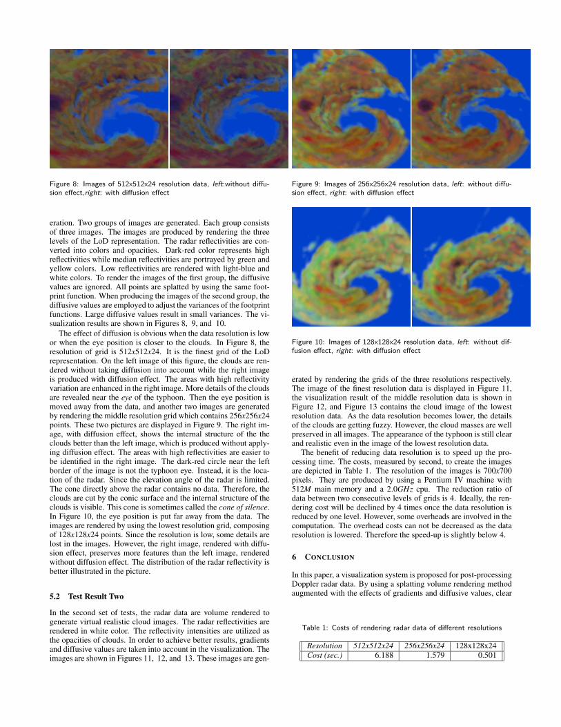
Figure 8: Images of 512x512x24 resolution data, left:without diffu-

sion effect,right: with diffusion effect

eration. Two groups of images are generated. Each group consistsof three images. The images are produced by rendering the threelevels of the LoD representation. The radar reflectivities are con-verted into colors and opacities. Dark-red color represents highreflectivities while median reflectivities are portrayed by green andyellow colors. Low reflectivities are rendered with light-blue andwhite colors. To render the images of the first group, the diffusivevalues are ignored. All points are splatted by using the same foot-print function. When producing the images of the second group, thediffusive values are employed to adjust the variances of the footprintfunctions. Large diffusive values result in small variances. The vi-sualization results are shown in Figures 8, 9, and 10.

The effect of diffusion is obvious when the data resolution is lowor when the eye position is closer to the clouds. In Figure 8, theresolution of grid is 512x512x24. It is the finest grid of the LoDrepresentation. On the left image of this figure, the clouds are ren-dered without taking diffusion into account while the right imageis produced with diffusion effect. The areas with high reflectivityvariation are enhanced in the right image. More details of the cloudsare revealed near the eye of the typhoon. Then the eye position ismoved away from the data, and another two images are generatedby rendering the middle resolution grid which contains 256x256x24points. These two pictures are displayed in Figure 9. The right im-age, with diffusion effect, shows the internal structure of the theclouds better than the left image, which is produced without apply-ing diffusion effect. The areas with high reflectivities are easier tobe identified in the right image. The dark-red circle near the leftborder of the image is not the typhoon eye. Instead, it is the loca-tion of the radar. Since the elevation angle of the radar is limited.The cone directly above the radar contains no data. Therefore, theclouds are cut by the conic surface and the internal structure of theclouds is visible. This cone is sometimes called the cone of silence.In Figure 10, the eye position is put far away from the data. Theimages are rendered by using the lowest resolution grid, composingof 128x128x24 points. Since the resolution is low, some details arelost in the images. However, the right image, rendered with diffu-sion effect, preserves more features than the left image, renderedwithout diffusion effect. The distribution of the radar reflectivity isbetter illustrated in the picture.

5.2 Test Result Two

In the second set of tests, the radar data are volume rendered togenerate virtual realistic cloud images. The radar reflectivities arerendered in white color. The reflectivity intensities are utilized asthe opacities of clouds. In order to achieve better results, gradientsand diffusive values are taken into account in the visualization. Theimages are shown in Figures 11, 12, and 13. These images are gen-

Figure 9: Images of 256x256x24 resolution data, left: without diffu-

sion effect, right: with diffusion effect

Figure 10: Images of 128x128x24 resolution data, left: without dif-

fusion effect, right: with diffusion effect

erated by rendering the grids of the three resolutions respectively.The image of the finest resolution data is displayed in Figure 11,the visualization result of the middle resolution data is shown inFigure 12, and Figure 13 contains the cloud image of the lowestresolution data. As the data resolution becomes lower, the detailsof the clouds are getting fuzzy. However, the cloud masses are wellpreserved in all images. The appearance of the typhoon is still clearand realistic even in the image of the lowest resolution data.

The benefit of reducing data resolution is to speed up the pro-cessing time. The costs, measured by second, to create the imagesare depicted in Table 1. The resolution of the images is 700x700pixels. They are produced by using a Pentium IV machine with512M main memory and a 2.0GHz cpu. The reduction ratio ofdata between two consecutive levels of grids is 4. Ideally, the ren-dering cost will be declined by 4 times once the data resolution isreduced by one level. However, some overheads are involved in thecomputation. The overhead costs can not be decreased as the dataresolution is lowered. Therefore the speed-up is slightly below 4.

6 CONCLUSION

In this paper, a visualization system is proposed for post-processingDoppler radar data. By using a splatting volume rendering methodaugmented with the effects of gradients and diffusive values, clear

Table 1: Costs of rendering radar data of different resolutions

Resolution 512x512x24 256x256x24 128x128x24Cost (sec.) 6.188 1.579 0.501

Figure 11: Cloud image of 512x512x24 resolution data

Figure 12: Cloud image of 256x256x24 resolution data

Figure 13: Cloud image of 128x128x24 resolution data

visualization results are achieved even when the images are gener-ated by rendering lower resolution data. Our system provides thecapacity of generating realistic cloud images and comprehensiblecolorful images. Therefore, the key features of the radar data areexplicitly revealed.

It takes minutes for a modern meteorological radar to completean entire scanning process. The time step between two consecu-tive scanning is too large to generate a smooth sequence of imagesfor animation. Therefore, interpolation procedures are required forestimating the movement and development of clouds between ev-ery two time steps. To achieve better accuracy, the velocity field inthe space should be taken into consideration for the interpolation.According to the Doppler shift effect, a Doppler radar can detectthe movement of a cloud mass. However, the velocity of the move-ment cannot be exactly measured except in the radial direction ofthe radar. Based on an optical flow computing method, we calculatethe velocity field of cloud. Then the velocities are rendered to showthe tendency of cloud motion. The velocities are also used to advectcloud particles to interpolate radar data at time points selected byusers.

The precipitation may be changed because of rain-fall, waterevaporation from the ground, and the advection of wind betweentwo time steps. In our current work, we ignore raining and evapo-ration effects to achieve quick results. Some models have been de-veloped to estimate rain-fall and evaporation and predict weather.However, these models are still not accurate enough for weatherforecasting. Complicated terrain also creates difficult for scanningdata by using Doppler radars. To overcome these problems is of thehighest priority in visualizing Doppler radar data.

REFERENCES

[1] C. Donald Ahrens. Meteorology Today. Brooks/Cole-Thomson Learn-ing, 2003.

[2] J. L. Beauchemin, S. S.and Barron. The Computation of Optical Flow.ACM Computing Surveys, 27(3):433–467, 1995.

[3] Byron R. Bird, Warren E. Stewart, and Edwin N. Lightfoot. TransportPhenomena. John Wiley & Sons, Inc., 1960.

[4] M Chong, J. F. Georgis, O. Bousquet, S. R. Brodzik, C. Burghart,S. Cosma, U. Germann, V. Gouget, R. A. Houze, C. N. James,S. Prieur, R. Rotunno, F. Froux, Vivekanandan, and Z. X. Zeng. Real-

Time Wind Synthesis from Doppler Radar Observations during theMesoscale Alpine Programme. Bulletin of the American Meteorolog-ical Society, 81(12):2953–2962, 2000.

[5] Paolo Cignoni, Claudio Montani, Enrico Puppa, and RobertsScopigno. Multiresolution Representation and Visualization of Vol-ume Data. IEEE Transactions on Visualization and Computer Graph-ics, 11:352–369, 1997.

[6] C. A. Clift. Use of Radar in Meteorology. World MeteorologicalOrganization, 1985.

[7] C. G. Collier. Application of Weather Radar Systems: A Guide to Usesof Radar Data. Halsted Press, 1989.

[8] Harry F. Davis and Arthur David Snider. Introduction to Vector Anal-ysis. Wm. C. Brown Publisher, 1991.

[9] Suzana Djurcilov and Alex Pang. Visualizing Gridded Datasets withLarge Number of Missing Values. In Proceedings of IEEE Visualiza-tion’1999, pages 405–408, 1999.

[10] Yoshinori Dobashi, Kazufumi Kaneda, Hideo Yamashita, TsuyoshiOkita, and Yomoyuki Nishita. A Simple, Efficient Method for Realis-tic Animation of Clouds. In Proceedings of SIGGRAPH 2000, pages19–28, 2000.

[11] Ronald Fedkiw, Jos Stam, and Henrik Wann Jensen. Visual Simulationof Smoke. In Proceedings of SIGGRAPH’01, pages 15–22, 2001.

[12] Nick Foster and Dimitris Metaxas. Modeling the Motion of a Hot,Turbulent Gas. In Proceedings of SIGGRAPH’97, pages 181–188,1997.

[13] Katja Friedrich and Martin Hagen. On the use of advanced Dopplerradar techniques to determine horizontal wind fields for operationalweather surveillance. Meteorological Applications, 11:155–171,2004.

[14] M. P. Garrity. Raytracing Irregular Volume Data. Computer Graphics,24:35–40, 1990.

[15] Thomas Gerstner, Dirk Meetschen, Susanne Crewell, MichaelGriebel, and Clemens Simmer. A Case Study on Multiresolution Vi-sualization of Local Rainfall from Weather Radar Measurements. InProceedings of IEEE Visualization’2002, pages 533–536, 2002.

[16] Mark Harris, William Baxter, Thorsten Scheuerman, and AnselmoLastra. Simulation of Cloud Dynamics on Graphics Hardware. In Pro-ceedings of SIGGRAPH/EUROGRAPHICS on Graphics Hardware2003, pages 92–101, 2003.

[17] Mark Harris and Anselmo Lastra. Real-Time Cloud Rendering. InProceedings of EUROGRAPHICS 2001 Conference, pages 76–84,2001.

[18] Elke Hergenrother, Antonio Bleile, Don Middleton, and AndrzejTrembilski. The Abalone Interpolation, A Visual Interpolation Pro-cedure for the Calculation of Cloud Movement. In Proceedings of theXV Brazilian Symposium on Computer Graphics and Image Process-ing, 2002.

[19] William Hibbard. Large Operational User of Visualization. ACM SIG-GRAPH Computer Graphics, 37(3):5–9, August 2003.

[20] William L. Hibbard. 4-D Display of Meteorological Data. In Proceed-ings of the 1986 Workshop on Interactive 3D Graphics, pages 23–36,1986.

[21] Justin Jang, William Ribarsky, Christopher Shaw, and Nickolas Faust.View-Dependent Multiresolution Splatting of Non-Uniform Data. InProceedings of IEEE TVCG Symposium on Visualization 2002, pages125–132, 2002.

[22] James Kajiya and Brian P. von Herzon. Ray Tracing Volume Densi-ties. In Proceedings of SIGGRAPH’84 Conference, pages 165–174,1984.

[23] Scott King, Roger Crawfis, and Wayland Reid. Fast Animation ofAmorphous and Gaseous Phenomena. In Proceedings of VolumeGraphics 1999, pages 333–346, 1999.

[24] David Laur and Pat Hanrahan. Hierarchical Splatting: A ProgressiveRefinement Algorithm for Volume Rendering. In Proceedings of SIG-GRAPH’91 Conference, July 1991.

[25] Nelson Max. Optical Models for Direct Volume Rendering. IEEETransactions on Visualization and Computer Graphics, 1(2):99–108,1995.

[26] Nelson Max, P. Hanrahan, and R. Crawfis. Area and Volume Coher-ence for Efficient Visualization of 3D Scalar Functions. ACM Com-

puter Graphics, 24:27–33, 1990.[27] Paula T. McCaslin, Philip A. McDonald, and Edward J. Szoke. 3D

Visualization Development at NOAA Forecast Systems Laboratory.ACM Computer Graphics, pages 41–44, February 2000.

[28] Ryo Miyazaki, Satoru Yoshida, Yoshinori Dobashi, and TomoyukiNishita. A Method for Modeling Clouds Based on Atmospheric FluidDynamics. In Proceeding of Pacific Graphics 2001 Conference, pages363–373, 2001.

[29] Tomoyuki Nishita, Yoshinori Dobashi, and Eihachro Nakamae. Dis-play of Clouds Taking into Account Multiple Anisotropic Scatteringand Sky. In Proceedings of SIGGRAPH’96, pages 379–386, 1996.

[30] Tomoyuki Nishita, Takao Sirai, Katsumi Tadamura, and EihachroNakamae. Display of Earth Taking into Account Atmospheric Scat-tering. In Proceedings of SIGGRAPH’93, pages 175–182, 1993.

[31] T. V. Papathomas, J. A. Schiavone, and B. Julesz. Applications ofComputer Graphics to the Visualization of Meteorological Data. ACMSIGGRAPH Computer Graphics, 22(4):327–334, August 1988.

[32] Holly Rushmeier and Kenneth Torrance. The Zonal Method for Cal-culating Light Intensities in the Presence of a Participating Medium.In Proceedings of SIGGRAPH’87, pages 293–302, 1987.

[33] Joshua Schpok, David Ebert, and Charles Hansen. A Real-Time CloudModeling, Rendering, and Animation System. In Proceedings of the2003 ACM SIGGRAPH/Eurographics Symposium on Computer Ani-mation, pages 160–166, 2003.

[34] Alan Shapiro, Paul Robinson, Joshua Wurman, and Jidong Gao.Single-Doppler Velocity Retrieval with Rapid-Scan Radar Data. Jour-nal of Atmospheric and Oceanic Technology, 20:1578–1595, 2003.

[35] Peter Shirley and Allan Tuchman. A Polygonal Approximation toDirect Scalar Volume Rendering. In Proceedings of 1990 Workshopon Volume Visualization, pages 63–70, December 1990.

[36] Lloyd A. Treinish. Visualization of Scattered Meteorological Data.IEEE Computer Graphics and Applications, 15(4):20–26, 1995.

[37] John Tuttle and Robert Gall. A Single-Radar Technique for Estimatingthe Winds in Tropical Cyclones. Bulletin of the American Meteoro-logical Society, 80(4):653–668, 1999.

[38] Shyh-Kuang Ueng. Out-of-Core Encoding of Large TetrahedralMeshes. In Proceedings of Eurographics/IEEE Volume GraphicsWorkshop, pages 95–102, 2003.

[39] Shyh-Kuang Ueng, Yan-Jen Su, and Ji-Tang Chang. LoD VolumeRendering of FEA Data. In Proceedings of IEEE Visualization’2004,pages 417–424, 2004.

[40] Lee Westover. Interactive Volume Rendering. In Proceedings of theChapel Hill Workshop on Volume Visualization, May 1989.

[41] Lee Westover. Footprint Evaluation for Volume Rendering. In Pro-ceedings of SIGGRAPH’90 Conference, August 1990.

[42] Matthias Zwicker, Hanspeter Pfister, Jeroen van Baar, and MarkusGross. EWA Volume Splatting. In Proceedings of IEEE Visualiza-tion’2001, pages 29–36, 2001.