820 IEEE TRANSACTIONS ON FUZZY SYSTEMS, VOL. 12, NO. 6, DECEMBER 2004

A Generalized Concept for Fuzzy Rule InterpolationPéter Baranyi, László T. Kóczy, and Tamás (Tom) D. Gedeon

Abstract—The concept of fuzzy rule interpolation in sparse rulebases was introduced in 1993. It has become a widely researchedtopic in recent years because of its unique merits in the topicof fuzzy rule base complexity reduction. The first implementedtechnique of fuzzy rule interpolation was termed as -cut dis-tance based fuzzy rule base interpolation. Despite its advantageousproperties in various approximation aspects and in complexityreduction, it was shown that it has some essential deficiencies, forinstance, it does not always result in immediately interpretablefuzzy membership functions. This fact inspired researchers todevelop various kinds of fuzzy rule interpolation techniques inorder to alleviate these deficiencies. This paper is an attempt intothis direction. It proposes an interpolation methodology, whosekey idea is based on the interpolation of relations instead of inter-polating -cut distances, and which offers a way to derive a familyof interpolation methods capable of eliminating some typicaldeficiencies of fuzzy rule interpolation techniques. The proposedconcept of interpolating relations is elaborated here using fuzzy-and semantic-relations. This paper presents numerical examples,in comparison with former approaches, to show the effectivenessof the proposed interpolation methodology.

Index Terms—Fuzzy rule interpolation, sparse fuzzy rule-base.

I. INTRODUCTION

THE concept of interpolating in sparse rule bases, termedas fuzzy rule interpolation, and its first implementation,

termed as -cut distance based fuzzy rule base interpolation( -cut interpolation shortly), were introduced in 1990/1991[26]–[30]. Despite the advantages of fuzzy rule interpolationin different issues of fuzzy theory shown in a number of arti-cles, it was also proved that the -cut interpolation does notaccommodate some elementary conditions of fuzzy concept incases. In this regard, conditions were investigated by Kovács[31]–[34], Kawase and Chen [25], and Shi and Mizumoto [47].As a result, three typical problems of interpolation have comeinto the focus of the related literature, which are addressedas abnormal conclusion, nonpreserving linearity, restrictionto convex normalized fuzzy (CNF) sets. Abnormal conclusion

Manuscript received August 22, 2000; revised June 13, 2002 and February20, 2004. This work was supported by the Hungarian Scientific Research Fund(OTKA) under Grants T 034233 and F 030056, by FKFP 180/2001 and NKFP-2/0015/2002, and by the Australian Research Council. The work of P. Baranyiwas supported by the Zoltán Magyary scholarship.

P. Baranyi is with the Computer and Automation Research Institute, the Hun-garian Academy of Sciences, and also with the Department of Telecommunica-tion and Media Informatics, Budapest University of Technology and Economics,and Integrated Engineering Systems Japanese-Hungarian Laboratory, BudapestH-1117, Hungary (e-mail: baranyi@alpha.ttt.bme.hu).

L. T. Kóczy is with the Department of Telecommunication and Media Infor-matics, Budapest University of Technology and Economics, and Integrated En-gineering Systems Japanese-Hungarian Laboratory, Budapest H-1117 (e-mail:koczy@ttt.bme.hu).

T. D. Gedeon is with the Department of Computer Science, The AustralianNational University, Acton ACT 0200, Australia (e-mail: tom@cs.anu.edu.au).

Digital Object Identifier 10.1109/TFUZZ.2004.836085

means that the interpolation yields at least two membershipvalues over at least one element of the output universe, orthe resulted membership values are not bounded by .Nonpreserving linearity is addressed when not piece-wiselinear conclusion is inferred from piece-wise linear rules andobservations. Restriction to CNF sets means the interpolationdoes not function with arbitrary type of fuzzy sets, but withCNF sets. Inspired by the purpose of eliminating these typicaldeficiencies in certain cases, various interpolation methodswere developed in the 1990s.

A. Brief Overview of Fuzzy Rule Interpolation Techniques

The explicit form of -cut interpolation, called the funda-mental equation of fuzzy rule interpolation, is actually a fuzzyextension of the classical linear interpolation of given points.The -cut interpolation method infers a conclusion based oncarrying the proportion of the fuzzy distances [30] between theobservation and the rule antecedents over the correspondingconsequents and the conclusion [26]–[29]. The fuzzy distanceutilized in the -cut interpolation reflects to some extent of theideas of approximate analogical reasoning proposed by Turksenin 1988 [53], and is actually a family of -cut distances. Thisis the reason why we call the first interpolation method -cutdistance based fuzzy rule interpolation [48], [61]. Accordingto the definition of the fuzzy distance, a class of methods canbe derived in the fashion of -cut interpolation. For instance,different definitions of distance were proposed by Vass et al.in [58] and [18]. It is remarkable that the method proposed in[18] eliminated the problem of abnormal conclusion, however,it did not function with certain crisp fuzzy sets. Its improvedversion was proposed in 1997. These techniques assume thatthe fuzzy premises and consequents are CNF sets. Let us groupthese approaches as -cut based methods. As a mater of fact,in the case of arbitrary shaped CNF sets theoretically an infinitenumber of -levels should be taken into account, in order, toyield a proper conclusion. To achieve an acceptable computa-tional requirement for practical cases one may restrict the com-putation to a finite number of -levels (usually three or four),after assuming that the fuzzy sets applied are piecewise linear,for instance triangular or trapezoidal shaped. Unfortunately, theaforementioned methods do not preserve linearity, which simplymeans that calculating the piecewise linear sets only at certain

-levels and connecting the resulting points of the conclusionby linear pieces yields an approximation of the accurate conclu-sion. The deviation of the piecewise linear approximation fromthe accurate conclusion is, however, dispensable in the case of

-cut interpolation, as pointed out in [48] and [31]–[34]. An-other method proposed by Dubois and Prade in [15]–[17] op-erated with all possible distances among the elements of fuzzysets at each -level and computed all corresponding elements

1063-6706/04$20.00 © 2004 IEEE

Authorized licensed use limited to: UNIVERSITY OF TOKYO. Downloaded on March 20, 2009 at 07:13 from IEEE Xplore. Restrictions apply.

BARANYI et al.: A GENERALIZED CONCEPT FOR FUZZY RULE INTERPOLATION 821

of the conclusion for the same -level. The membership func-tion of the conclusion is obtained here by bounding the resultingelements at each -level. In contrast with the aforementionedmethods, Dubois and Prade’s method was the first one, whichcould be applied to rule-bases, which were not restricted to CNFsets, as stated in [19]. As opposed to this advantage, Duboisand Prade’s method might yield abnormal conclusion in cer-tain cases [19]. In view of its essence, this approach is also in-cluded in the group of -cut based methods. In order to keep thesimplicity of -cut interpolation, but to eliminate the problemof abnormal conclusion, papers [7] and [8] propose the trans-formation of the fundamental equation of -cut interpolationto the space of normal conclusions. This method was termedmodified -cut interpolation. Shortly afterwards, Tikk et al. an-alyzed its various properties in [48]. It was shown that it also didnot preserve linearity, but the deviation of the piecewise linearconclusion from the accurate one was less than in the case of

-cut interpolation. Tikk et al. also showed that the modifiedmethod inherited the approximation stability of the -cut inter-polation [49], [50]. The modified -cut method was extended tononconvex fuzzy sets by Tikk et al. in [52]. One of the recentmethods of this narrow topic uses the combination of differentinterpolation techniques proposed by Wong et al. [60], [61].

In 1995, a conceptually different method was introducedby the authors [1]–[6]. It was termed “solid cutting method”and “generalized interpolation method.” Its essential differencefrom the former approaches is that this method infers theconclusion based on the interpolation of relations instead of

-cut distances. It has two main steps. In the first step a ruleis interpolated from the rule-base as “close” to the observationas possible, based on a spatial solid cutting technique. Theterm “close” means here that at least partial overlapping isensured between the observation and the interpolated rule,which implies the firing of the interpolated rule. In the secondstep, the conclusion is inferred from the consequent of the firedrule according to the similarity between the observation andthe interpolated antecedent. The advantage of this method isthat it is applicable to arbitrary shaped sets and does not yieldabnormal conclusion. This method can readily be extended tofuzzy rule extrapolation as detailed in [5]. The drawback of thismethod is its high computational complexity. Some practicalsimplifications of this method have been done for piece-wiselinear fuzzy sets [40]–[42]. These simplified methods preservelinearity. In 1997, the authors replaced the fuzzy interpolationin the first step by the interpolation algorithm of semantic rela-tions [6]. Simultaneously, Kawaguchi et al. proposed a B-splinetechnique based fuzzy interpolation method in [21]–[24], whichcould be viewed as a kind of generalization of the first step.Kawaguchi’s method functions with fuzzy sets given by afinite number of characteristic points. Let these algorithms beincluded in a group named generalized methods.

In 1997, Yam introduced a vector based approach to representmembership functions as points in high-dimensional Cartesianspace [54]–[57]. This method transforms the ideas of fuzzy ruleinterpolation to the interpolation of vector mapping. A recentvariation was proposed in [54], which we include in the groupof generalized methods since it is constructed by the two steps ofthe generalized concept in terms of matrix operations. However,

it is restricted to sets given by a finite number of characteristicpoints.

Various further techniques have been proposed in the lastyears. For instance Bouchon-Meunier introduced the gradualitybased interpolative reasoning [9]–[11]. Kóczy and Hirota andothers published results about the use of -cut interpolationin hierarchically structured rule-bases [35], [44]. Mizik et al.compared various interpolation techniques in a uniform descrip-tion [40]–[42]. In 1996, Kovács et al. proposed an interpola-tion technique based on the approximation of the vague envi-ronment of fuzzy rules and applied it in the control of an au-tomatic guided vehicle system [36]–[38]. Jenei introduced anaxiomatic treatment of linear interpolation and extrapolation asa new way of interpolation of compact fuzzy quantities and pro-posed its multi-dimensional extension in [19], [20]. He also in-vestigated various properties of interpolation techniques. Bou-chon-Meunier proposed a comparative view of fuzzy interpola-tion methods in [12].

B. Aim of this Paper

The aim of this paper is to introduce a methodology for fuzzyrule interpolation. This methodology has already been partiallyinitialized by the authors in [1]–[6]. Further, this interpolationmethodology is capable of eliminating typical deficienciesof fuzzy interpolation methods. By the help of the proposedmethodology a class of linear and nonlinear fuzzy interpolationmethods can be developed. The key idea of this interpolationmethodology is based on the interpolation of relations. As animplementation, two groups of algorithms are developed in thispaper. One is based on the interpolation of fuzzy relation. Theother is based on the interpolation of semantic relation. Thecomparison of the resulting interpolation methods to the formertechniques is given in this paper. Various further comparisonhave already been published. Detailed comparisons, by Mizik[40]–[42], Tikk et al. [48] and by the authors, analyze the -cut,the modified -cut interpolation and solid cutting method in auniform coordinate system. Further, [19] compares the -cutbased interpolation, Dubois and Prade’s technique and thesolid cutting method. Consequently, all the results of thesecomparisons, done for the preliminary works such as solidcutting method and the revision principle based technique, canstraightforwardly be carried over the interpolation method-ology which will be discussed in this paper. Some, numericalexamples are investigated both in this paper and in [1] and [2].

II. DEFINITIONS AND NOTATION

This section introduces some elementary definitions and con-cepts utilized in the further developments. Before starting withthe definitions, some comments are enumerated on the notation.To facilitate the distinction between the types of given quanti-ties, they will be reflected by their representation: scalar valuesare denoted by lower-case letters ; fuzzy sets by cap-ital letters as ; and letter is reserved to denotefuzzy rule IF , THEN , briefly . Letters ,and are, respectively, reserved to input–output universes andto the third dimension of geometrical representation, see later.In order to enhance the overall readability characters

Authorized licensed use limited to: UNIVERSITY OF TOKYO. Downloaded on March 20, 2009 at 07:13 from IEEE Xplore. Restrictions apply.

822 IEEE TRANSACTIONS ON FUZZY SYSTEMS, VOL. 12, NO. 6, DECEMBER 2004

are in the meaning of subscripts (counters), and arereserved to denote the respective upper bounds of the subscripts,unless stated otherwise. Further, is assigned to the index offuzzy rules. The membership functions of the fuzzy sets usedthrough this paper are continuous with bounded support. An-tecedent fuzzy sets are denoted by ; consequent setsby . Notations and are for the observation andconclusion, respectively. Superscript indicates that the givenquantity being “interpolated”. Notations simply mean thelower and upper bound of . is an interpolation pa-rameter.

Definition 1 (Lower and Upper Bound of Fuzzy Set): Given fuzzy set . The lower and upper bounds

of in are given by support and support .Definition 2 (Centre Point of Fuzzy Set ): The

center point of a given fuzzy set is:, where height . denotes the -cut of

.Definition 3 (Normal Fuzzy Set): A fuzzy set is normal if

it has at least one element whose membership value is one.Definition 4 (Subnormal Fuzzy Set): A fuzzy set is sub-

normal if it does not have any elements whose membershipvalue is one.

The next Definition 5 is used to describe the relation betweenthe elements of two universes. Its idea is actually taken fromthe so called revision principle, where the relation is defined asthe revision function or interrelation function (see [13], [14],[43], [45], and [46]). In this paper, a piecewise linear variant isutilized.

Definition 5 (Piecewise Linear Interrelation Func-tion): , where

, where and ,and , where and

, subject to . The interrelationfunction is a piecewise linear function where the linear piecesare defined by point-pairs . Fig. 1 depicts an inter-relation function, where , namely, the vector consistsof four elements.

The interrelation function is used to assign the nonzero mem-bership valued elements of sets and of a rule .

Definition 6 (Interrelation Area): The interrelation area ofinterrelation function is a rectangular area defined by pointswhich the interrelation function ends in, namely, by pointsand ; see Figs. 1, 15, and 16. This can also be implementedas the area defined by the support of antecedent and conse-quent of a rule .

Definition 7 (Linear Interpolation of Two Points): Function, is the linear

interpolation between given and (superscript denotes“interpolated”).

III. KEY IDEA OF THE GENERAL FUZZY INTERPOLATION

METHODOLOGY

This section is intended to introduce the fundamental con-cept of the generalized method. To capture the main idea,first interpolation in a one variable rule-base is discussed in

Fig. 1. Linear interrelation function y = �(x;p ;p ).

Sections IV–VII. Multidimensional extension is treated inSections VIII and IX. The discussion of this paper is restrictedto the elementary step of interpolation, namely, to the interpo-lation between two rules selected from the rule-base. In orderto avoid overlapping with preliminary papers, the way of se-lecting two rules is not in focus here. For the sake of simplicity,let us assume that the rule selection is done by the selectiontechnique proposed for the -cut interpolation. In order toinitialize further discussion, let the following assumptions andstatements be recalled from [29], [30], [48], and [54]. Thevariables, including input universe and output universe arebounded and gradual in the sense of [15]. So, a linear orderingin each of them exists. In this case, a partial ordering can beintroduced among the elements of and . Having this partialordering between , denoted by , if andare comparable, i.e., , it is possible to define a distancebetween these two fuzzy sets that will be denoted by .Assume that an observation is given, towhich the conclusion is searched for.Further, assume that two fuzzy rules are selected so that

and

and

where and .In the following, the main steps of the proposed method are

presented.

A. Generalized Method for Fuzzy Rule Interpolation

1) Generation of an Interpolated Firing Rule: In this step,an interpolated rule is generated, which is locatedbetween and , in such a way that is as “close” to aspossible, but in any case it has at least partial overlapping with

. For brevity, let this step be denoted by

(1)

Authorized licensed use limited to: UNIVERSITY OF TOKYO. Downloaded on March 20, 2009 at 07:13 from IEEE Xplore. Restrictions apply.

BARANYI et al.: A GENERALIZED CONCEPT FOR FUZZY RULE INTERPOLATION 823

where is a mapping from pairs of - rulesinto the set of possible - rules.

. As a matter of fact, this definitionof “closeness” and the degree overlapping can be selected ina suitable way rather freely, but shall, be used later on consis-tently.

2) Inference of the Conclusion: Let the newly generated in-terpolated rule be considered temporarily as if it were one ofthe existing rules of the rule-base. The overlapping of the ob-servation and the interpolated antecedent implies the firing ofthe interpolated rule. Let this step be denoted as

Remark 1: Various algorithms introduced in the related lit-erature can be substituted into the above steps and analyzed inregards to the three typical deficiencies of the fundamental ver-sions of interpolation discussed in the first paragraph of the In-troduction. For instance, Kawaguchi’s B-spline based rule inter-polation is directly substitutable into the first step. Its immediateconsequence is that the method obtained in this way inheritsrestriction to piecewise fuzzy sets given by a finite number ofpieces. In the case of the second step, single rule reasoning tech-niques have prominent roles. For instance, the use of the revisionprinciple introduced by Shen et al. are detailed in this paper.

B. Further Characterization

This section introduces further characterizations for theoverall view of fuzzy interpolation. In [7], [8], [40]–[42], and[48], a technique is presented that is capable of comparingdifferent interpolation methods in a uniform coordinate system.This technique implicitly determines a generable usable refer-ence point for the fuzzy sets in the rules. Let a reference pointof a fuzzy set be defined by Definition 8 as follows.

Definition 8 (Reference Point : is a point ofassigned to fuzzy set , so that expresses the “most

typical“ location of fuzzy set . in everycase. It could be, for instance, some kind of defuzzified value of

.The use of the idea of reference point helps with examining

the global feature of the interpolations via simplified explicitforms. A global feature of the interpolation can, hence, be de-scribed by the function of the reference points of the inferredconclusions with respect to the reference points of the observa-tions; see Figs. 9 and 10. Let this function be termed as follows.

Definition 9 (Interpolation Generatrix): Let the interpola-tion generatrix be the function of the observation in re-spect to conclusion , such that and ,whenever andbeing the rule base interpolation function.

For example, if fuzzy numbers are used in -cut interpola-tion and is fixed for all sets, then the interpola-tion generatrix between two neighboring rules is a straight lineshowing the linear feature of the -cut interpolation. In this case,the set of points defined by the cut of all the possible ob-servations and conclusions equals the interpolation generatrix.

One of the aims of this paper is to propose various algorithmsfor the implementation of the interpolation method. Before

dealing with the algorithms in detail a brief digression needs tobe taken here to define a concept of “closeness” by introducinga simple distance between two fuzzy sets that will be used lateron in this paper. Let

which is a crisp distance in contrast with -cut distance-basedmethods. Without the loss of generality let in this paper the ref-erence point be fixed to the center point, so that

(2)

is used from now on. Therefore, if thenand will be comparable, i.e., we write . Let theinterpolated rule be determined subject to

(3)

which ensures an overlapping between and . Again therestrictions in (2) and (3), are not necessary for the interpolationmethod in general, it can be set in various ways rather freely.Equations (2) and (3) have been chosen for the implementations,detailed in the next sections, of the interpolation method.

IV. RULE INTERPOLATION

Two groups of algorithms are introduced in this section aspossible implementations of the first step of the proposed in-terpolation method. The first group is based on fuzzy relationinterpolation, the second one is based on semantic relation in-terpolation.

A. Fuzzy Relation Interpolation

The first algorithm in this group is the detailed version ofthe solid cutting method proposed by the authors in [1]–[5].The second and the third algorithms respectively apply the fixedpoint law (FPL) and the fixed value law (FVL) theory, intro-duced by Shen et al. [13], [14], [43], [45], [46], to fuzzy setinterpolation. The essential difference between FPL and FVLalgorithms is that the FPL method considers the membershipvalues, while the FVL operates with the “fuzziness” of the sets,see later. Fuzzy relation interpolation is computed here via in-terpolating the fuzzy sets

and

where

where . First, the fuzzy set interpolation tech-niques will be proposed and then the fuzzy relation interpola-tion algorithm will be introduced.

Algorithm 1 (Solid Cutting (SC) Fuzzy Set Interpolation):

Let (dimension is orthogonal onon Figs. 2 and 3), be the function (see

Figs. 2 and 3) that is obtained by rotating the membership func-tion by 90 around the axis that is positionedat . Let a solid

Authorized licensed use limited to: UNIVERSITY OF TOKYO. Downloaded on March 20, 2009 at 07:13 from IEEE Xplore. Restrictions apply.

824 IEEE TRANSACTIONS ON FUZZY SYSTEMS, VOL. 12, NO. 6, DECEMBER 2004

Fig. 2. Interpolating fuzzy sets by solid cutting.

be constructed by fitting a surface on generatrices . Letbe the cross-section of this imagined solid at position

, where . Turningback into its original position the interpolated fuzzy set

is obtained.Great variety of algorithms capable of fitting a surface to the

generatrices can be defined according to specific de-sired properties. Regarding the length of this paper only one al-gorithm is discussed here as a possible solution. Let such analgorithm be developed here which holds the following proper-ties.

Property 1 (Compatibility With the Rule Base): The intersec-tion of the solid at points and must, respectively,be equivalent to and . This meansthat if , then and if , then .

Property 2 (Avoiding Abnormal Fuzzy Set): The intersec-tion of the solid at any points is a function and bounded by [0,1]. This simply means that all intersections are interpretable asfuzzy sets.

Property 3 (Normalization): If and are normalizedfuzzy sets (Definition 3) then the interpolated fuzzy set is anormalized fuzzy set.

Property 4 (Preserving Linearity): If and are givenby the same number of linear pieces then the interpolated set isalso a piecewise linear set.

The surface of the imagined solid is created by simple conicaland cylindrical line surfaces in the next part of this section. Inorder to facilitate further discussion first the key steps are illus-trated on a simple example.

Step 1) Let the generatrices be divided into piecesby characteristic points. These pieces will determinethe bound of the conical and the cylindrical line sur-faces. As an example, Fig. 3 shows that function

and are divided by fiveand three points, respectively.

Step 2) Let the characteristic points be assigned betweengeneratrices . Following the example onFig. 3 let the characteristic points be assigned as

and.

Step 3) Those characteristic points, which are assigned toone, determine a conical surface and other pairs ofpoints determine the bound of a cylindrical surface.For example points and surround aconical surface. Similarly, points and

Fig. 3. Assigning the characteristic points.

also determine a conical surface. Cylindrical sur-faces are bounded by points and

.The following proposes possible solutions for the above three

steps. Let the characteristic points, discussed in Step 1), be de-fined by the following conditions

i) Let and , namely, the first and the lastcharacteristic points be those ones, which are corre-sponding to the lower and the upper bound of .Therefore, and

.ii) Those elements of the generatrices, which corre-

spond to the minimum and the maximum elementsof , where , are chosen to becharacteristic points as:

and .iii) Let also be included among the character-

istic points.iv) Let and the end points of the linear

pieces in the rotated membership function also beselected for characteristic points.

v) Those points where the function hasbreak points (where functionis not continuous) are also defined as characteristicpoints.

vi) Local minimum and maximum points of, like on Fig. 3, can also be con-

sidered as characteristic points.vii) Inflexion points of the generatrix are also taken into

account as characteristic points.Among the characteristic points of a generatrix there are

four distinguished ones, defined under points i) and ii), suchas and . According to these points letthe characteristic points of the th generatrix be divided intothree groups. Group consists of points ,where . Similarly: let ,where and , where

(note that points andare included in two groups). Let the process of Step 2) bestarted by assigning the distinguished characteristic points as

and , whichensures Property 3, because the assigned points will be con-nected by straight lines contained in the surface of the solid,see later. Therefore, if both rotated antecedents are normalizedthen at least one of these lines is parallel with the plane

Authorized licensed use limited to: UNIVERSITY OF TOKYO. Downloaded on March 20, 2009 at 07:13 from IEEE Xplore. Restrictions apply.

BARANYI et al.: A GENERALIZED CONCEPT FOR FUZZY RULE INTERPOLATION 825

Fig. 4. Topology of the characteristic points.

and lies at level . This implies that any intersectionof the solid has at least one point which coordinate equalsone, the interpolated set, hence, is normalized. The remainingcharacteristic points are assigned between the same numberedgroups, namely the points of are assigned to the pointsof . The point pairs between the groups are defined inthe same way for all . Fig. 4 shows an examplewhere group of the generatrices are depicted. Assumethat the number of points in is less than in . Thepoint pairs are simultaneously determined from the left andfrom the right side (see Fig. 4(a)) where pointsand are assigned first. Then the next two pointsare assigned from left and right, see pointsand . This is repeated until there is no morepoint or only one point remains in [Fig. 4(b)]. If thereis no more point in then the points connected last in theright and the left side are connected to the remaining pointsin . Namely, simultaneously one remaining point fromright side in connected to right point in and the leftremaining point in is connected to the left point in ,see Fig. 4(a) and (b). If the number of points in is oddthen the last point in is connected with the both pointsconnected last in as shown in Fig. 4(c). If the number ofpoint in is odd, namely, one point is remained then thispoint is connected with all remaining point in as depicted

Fig. 5. Cylindrical surface.

Fig. 6. Conical surface.

on Fig. 4(c). Fig. 4 shows that the topology of the connectionsyields triangular and quadrangular forms. The triangular formsare covered by simple conical surfaces and the quadrangularforms are covered by cylindrical surfaces. The cylindricalsurface is a line surface fit to two generatrices, where all pointsof the generatrices are connected by lines. Fig. 5 shows anexample, where point andare connected. Let the relation between and be defined as:

. In the caseof a conical surface, all points of the generatrix are connectedto one point; see Fig. 6.

The previously outlined technique holds Properties 1–4. Ad-ditionally, Property 5 can also be observed.

Property 5 (Continuity): For there existssuch that if , then for the in-tersections of the solid at and we have

. Therefore,if then, where and

.Property 5 comes from the fact that the solid is constructed by

continuous line surfaces. As a matter of fact, the characteristicpoints can be assigned in various ways. All assigning may resultin different solids. All solids have restrictions and advantageson their own. Our future work is to investigate the features ofvarious kinds of techniques capable of generating a solid basedon the given generatrices.

Authorized licensed use limited to: UNIVERSITY OF TOKYO. Downloaded on March 20, 2009 at 07:13 from IEEE Xplore. Restrictions apply.

826 IEEE TRANSACTIONS ON FUZZY SYSTEMS, VOL. 12, NO. 6, DECEMBER 2004

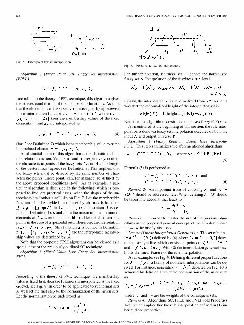
Fig. 7. Fixed point law set interpolation.

Algorithm 2 (Fixed Point Law Fuzzy Set Interpolation(FPLI)):

According to the theory of FPL technique, this algorithm givesthe convex combination of the membership functions. Assumethat the elements of fuzzy sets are assigned by a piecewiselinear interrelation function , where

then the membership values of the fixedelements and are interpolated as

(4)

(for see Definition 7) which is the membership value over theinterpolated element .

A substantial point of this algorithm is the definition of theinterrelation function. Vectors and , respectively, containthe characteristic points of the fuzzy sets and . The lengthof the vectors must agree, see Definition 3. This implies, thatthe fuzzy sets must be divided by the same number of char-acteristic points. These points can, for instance, be defined bythe above proposed conditions i)–vi). As an example, a par-ticular algorithm is discussed in the following, which is pro-posed to frequent practical cases, when the shapes of the an-tecedents are “rather nice” like on Fig. 7. Let the membershipfunction of be divided into pieces by characteristic points

and (notation is de-fined in Definition 1). and are the maximum and minimumelements of , where , like the characteristicpoints in the case of trapezoidal sets. Therefore, the interrelationis , (this function is defined in Definition5) and the interpolated member-ship values are determined by (4).

Note that the proposed FPLI algorithm can be viewed as aspecial case of the previously outlined SC technique.

Algorithm 3 (Fixed Value Law Fuzzy Set InterpolationFVLI):

According to the theory of FVL technique, the membershipvalue is fixed first, then the fuzziness is interpolated at the fixed

-level, see Fig. 8. In order to be applicable to subnormal setsas well let the first step be the normalization of the given sets.Let the normalization be understood as

height

Fig. 8. Fixed value law set interpolation.

For further notation, let fuzzy set denote the normalizedfuzzy set . Interpolation of the fuzziness at level

Finally, the interpolated is renormalized from in such away that the renormalized height of the interpolated set is

height

Note that this algorithm is restricted to convex fuzzy (CF) sets.As mentioned at the beginning of this section, the rule inter-

polation is done via fuzzy set interpolation executed on both theinput and output universe .

Algorithm 4 (Fuzzy Relation Based Rule Interpola-tion): This step summarizes the aforementioned algorithms

where

(5)

Formula (5) is performed as

and

(6)

Remark 2: An important issue of choosing andshould be addressed here. When defining , (3) should

be taken into account, that leads to

Remark 3: In order to master the use of the previous algo-rithms in the proposed general concept let the simplest choice

be briefly discussed.Lemma (Linear Interpolation Generatrix): The set of points

defined by (6) where deter-mine a straight line which consists of pointsand . With (2) the interpolation generatrix ex-hibits the linear feature of the rule interpolation.

As an example, see Fig. 9. Defining different proper functionsfor a family of nonlinear interpolations can be de-rived. For instance, generatrix depicted on Fig. 10 isachieved by defining a weighted combination of the rules suchas

where and are the weights of the consequent sets.Remark 4: Algorithms SC, FPLI, and FVLI hold Properties

1–5, which implies that the rule interpolation defined in (1) in-herits these properties.

Authorized licensed use limited to: UNIVERSITY OF TOKYO. Downloaded on March 20, 2009 at 07:13 from IEEE Xplore. Restrictions apply.

BARANYI et al.: A GENERALIZED CONCEPT FOR FUZZY RULE INTERPOLATION 827

Fig. 9. Linear interpolation.

Fig. 10. Nonlinear interpolation.

B. Semantic Relation Interpolation

This section uses the ideas of semantic revision principletechniques to describe the relation between antecedents andconsequent sets via semantic interpretation. Analogously tothe revision principle methods FPL and FVL, two kinds ofsemantic revision methods (SRM) have been introduced byShen et al. [13], [14], [43], [45], [46]. They are termed asSRM-I and SRM-II. Both techniques define an interrelationbetween the elements of fuzzy sets and a semantic relationfunction to capture the similarities of the membership values.In the case of SRM-I the element pairs, whose membershipvalues are recorded into a semantic function, are predefined byinterrelation function, which implies that the idea of the FPL isfollowed. As opposed to this in the case of the SRM-II, first themembership values are assigned by semantic function and then,according to this assignment, the interrelation function recordsthe fuzziness of the sets. This idea emerges in the FVL methods.Consequently, it can be concluded that the SRM methods arethe extensions of the FPL and the FVL in this sense. For moredetails, see [13], [14], [43], [45], and [46]. In order to facilitatethe undersatnding of the semantic relation based interpolation,first the basics of SRM methods is recalled.

Definition 10 (Semantics and Interrelation for SRM-I):

a) Interrelation:

Fig. 11. Interrelation and semantic relation of SMR-I.

Fig. 12. Interrelation and semantic relation of SMR-II.

b) Semantic relation:

For an illustration, see Fig. 11.Definition 11 (Semantics and Interrelation for SRM-II):

a) Semantic relation:

(7)

b) Interrelation:

For an illustration, see Fig. 12.In the next part, one more interpolation technique is proposed.

Its aim is to compute the interpolated semantic and interrelationfunctions to the observation as

(8)

Notations “-I” and “-II” utilized in the next algorithms are re-served to indicate that the concept of SRM-I or SRM-II is ap-plied.

Authorized licensed use limited to: UNIVERSITY OF TOKYO. Downloaded on March 20, 2009 at 07:13 from IEEE Xplore. Restrictions apply.

828 IEEE TRANSACTIONS ON FUZZY SYSTEMS, VOL. 12, NO. 6, DECEMBER 2004

Algorithm 5 (Interpolation of Semantic Relation, IS-I):

a) Interrelation:

b) Semantic relation:

Algorithm 6 (Interpolation of Semantic Relation,IS-II): Along the same line as in the case of FVL interpolationlet the semantic relations be normalized first. Therefore, let

(9)

where (I/II) means that the equation applicable for both IS-I andIS-II, and denotes normalized , which is in

fact means the same as the of the normalized setsand . Note that, if the sets are normalized, then their semanticrelations equal the set of points defined by , see (7) and(9). This implies that the semantic relations become equivalentfor all the rules in the case of IS-II.

a) Semantic relation

b) InterrelationIn order to give graphical interpretation of the interpola-tion let the interpretation of SRM-II be particularly mod-ified here. Let the points of and be de-fined in three dimensional space spanned by , andas

An illustration is given in Fig. 13.The interpolation can easily be defined in the three-dimen-

sional space as

Fig. 14 shows the interpolation of the interrelation fuctions.

Fig. 13. Illutsration of three dimensional IR .

Fig. 14. Interpolation of the interrelation function.

Similar to the case of FVLI algorithm, the final step is torenormalize the interpolated sets, namely, to renormalize the se-mantic relation function based on (8)

In order to use the semantic interpolation techniques in the pro-posed general concept the determination of and will beaddressed. The same conclusions can be drawn here as at thediscussion of fuzzy relation based interpolation algorithms. Let

according to (3). In the case ofglobally linear featured interpolation, is chosen. Again,like in the case of fuzzy relation-based interpolation, the equa-tion

(10)

determines the global feature of the interpolation, where (10) isdefined according to a desired interpolation generatrix.

V. SINGLE RULE INFERENCE

The objective of this section is to propose three kinds of tech-niques capable of firing the interpolated rule with the obser-vation and inferring the conclusion. These algorithms are forthe second step of the generalized interpolation method pro-posed in Section III. Single rule reasoning approaches, hence,

Authorized licensed use limited to: UNIVERSITY OF TOKYO. Downloaded on March 20, 2009 at 07:13 from IEEE Xplore. Restrictions apply.

BARANYI et al.: A GENERALIZED CONCEPT FOR FUZZY RULE INTERPOLATION 829

have prominent roles in this section. The proposed inference al-gorithms of this section are originated from the FPL, SRM-I,and SRM-II single rule inference methods [13], [14], [43], [45],[46], which have been developed for such cases when the sup-port of the observation consists of all elements and only thoseelements, which are contained in the interrelation function ofthe fired rule. Namely, the interrelation area (Definition 6) ofthe interpolated rule should agree with the support of the obser-vation. The interpolated relation (fuzzy or semantic), however,may not fulfill this condition. Therefore, this section introduceshow to expand the interpolated relation, in order, to match the re-quired area defined by the observation. This fitting ensures theproper matching of the interpolated relation with the observa-tion. First, an algorithm is proposed capable of transforming theinterrelation area of the interpolated relation to the observation.Then two algorithms, a fuzzy and a semantic relation-based,are discussed which transform the interpolated relation to thetransformed interrelation area. The use of these transformationsmeans that the interpolated relation is expanded in the “near”neighborhood of the observation. This is based on the assump-tion that the resulting relation is an acceptable approximation ofthe relation of this area.

Definition 12 [Spanning the Interrelation Area]: Assume that a fuzzy rule is given.

Its rectangular interrelated area is defined by intervalsand . The new area, which is proportionally spanned toa given interval is defined by intervals and as

and

Fig. 15 gives an illustration how the interrelation area is trans-formed.

The fuzzy and the semantic relation defined over the interre-lation area can be proportionally transformed accordingly to thespanning of the interrelation area. First, a fuzzy relation then asemantic relation based transformation are proposed.

A. Transformation of Fuzzy Relation

The fuzzy relation is transformed via set transformations onboth the input and the output universe.

Transformation 1 [Transformation of the Fuzzy Relation toa Given Interrelation Area ]: Assumefuzzy rule . Let fuzzy rulebe a transformed fuzzy rule whose interrelation area isdefined by and . Superscript means that “trans-formed.” The transformed antecedent set is determined as

, whereand . As a result and

. The consequent set is calculated in the same wayas: , whereand , which leads to and .

An illustration of the transformation is given in Fig. 16.

B. Transformation of Semantic Relation

The following transformation technique is applicable to thesemantic relation and results in a proportionally enlarged se-

Fig. 15. Spanned interrelation area.

Fig. 16. How A and B are defined according to the new interrelation area.

mantic relation which fits the new interrelation area. In this caseonly the transformation of the interrelation is of interest, sincethe semantic relation is independent on the size of the interre-lation area. This also implies that, the same transformation canbe proposed for methods I and II.

Transformation 2 (Transformation of the Semantic Rela-tion to a Given Interrelation Area): Assume that

and (let and respectively beused for brevity) are given. Let be the trans-formed interrelation function to a given interrelation areadefined by and as

, where

and . The semantic relation is not changedby the transformation, so, .

Note that both Transformations 1 and 2 hold Properties 1–5.For instance, if the interpolated antecedent equals to the obser-vation, then the transformed set equals the interpolated set. Thetransformations conserve piecewise linearity and normality. Thetransformation is continuous.

According to the previous section, the relations are interpo-lated to the observation in such a way that (3) is held. Again,in the second step the interrelation area and the interpolatedrelation is transformed to the observation. Finally, the conclu-

Authorized licensed use limited to: UNIVERSITY OF TOKYO. Downloaded on March 20, 2009 at 07:13 from IEEE Xplore. Restrictions apply.

830 IEEE TRANSACTIONS ON FUZZY SYSTEMS, VOL. 12, NO. 6, DECEMBER 2004

sion is generated from the transformed relation and the obser-vation after the transformed relation is assumed to be a goodapproximation of the interpolated relation. Having the trans-formed fuzzy and semantic relation immediately leads to the useof the revision principle methods, namely the FPL, SRM-I, andII single rule inference techniques. These methods are slightlyspecialized here according to (3). For further discussion let usassume that is transformed to the support of , namely,

has already been calculated from .In order to facilitate the notation “ ” (transformed) and “ ” (in-terpolated) is not used in the next part, the interpolated and trans-formed single rule to be fired is simply denoted as .The conclusion is generated by the following methods.

C. Inference by Fuzzy Relation

Algorithm (Inference of the Conclusion by FPL,): This algorithm fires the transformed fuzzy

relation. Performing the ideas of FPL, the membership func-tions are compared over each interrelated element of the sets.The deviation between the transformed antecedent and theobservation over a fixed element is carried to the interrelatedelement on the output universe to yield the deviation of theconclusion from the consequent. Considering all elements ofthe sets results in the membership function of the conclusion

and

Elements and are assigned by the transformed interrelationfunction.

D. Inference by Semantic Relation

Two semantic revision based methods are discussed in thenext part, namely, the concepts of SRM-I and II-based inferencetechniques, which are capable of concluding in respect tobased on the transformed semantic relation. These algorithmshave originally been developed for CNF sets and are slightlyspecialised here to . One more important con-dition of the SRM methods should be taken into account here.The inference by SRM methods assumes that heightheight which is, as a matter of fact, not ensured by any ofthe previous steps for all cases. Because of this let the semanticrelations be normalized in the same way as in the case of IS-II[see (9)].

Algorithm 7 (Inference by SRM-I,

, from [45]): The essential point is to carry the se-mantic and interrelation of the fired rule over the observationand the conclusion.

a) and .

Then, for all , the following holds.b) The conclusion is found by simply solving the following

equation for :

where andor .

Algorithm 8 (Inference by SRM-II,

, from [45]): Following the same idea as before,let

a) .The next two steps are solved for all .

b) , and .c) .

If the fired relation is normalized, then the above obtained con-clusion should be renormalized to the height of

height height

where height and

height

Note that these inference techniques keep Properties 1–3 and 5.Property 4 is guaranteed in the case of triangular shaped inter-polated rules.

VI. DISCUSSION OF THE PROPOSED ALGORITHMS

The previous sections proposed a generalized fuzzy rule in-terpolation method, and few techniques as examples for possibleimplementation. Let the generalized fuzzy rule interpolation bedenoted as

where indicates whichinterpolation technique is used and

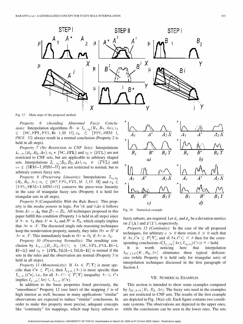
defines the single rule inference technique appliedin the second step of the method. This section is intended toinvestigate some properties of the interpolation methods imple-mented by the proposed algorithms. Special attention is paid onthe three typical deficiencies of interpolation methods discussedin the first paragraph of the Introduction. First of all, let themain steps be summarized and simply demonstrated via theSC interpolation method, namely, .Fig. 17 demonstrates the essential points of the concept.Assume that fuzzy rules , and obser-vation are given. In the first step a fuzzy ruleis interpolated in such a way that , namely,

(see (3), and note thatis set in (2)). In other words, the rule-base is interpolated atthe observation. The SC interpolation algorithm is actually ex-ecuted on the fuzzy sets. Both the interpolated antecedent andconsequent sets are generated by the solid cutting technique,see Fig. 17. The interpolated rule overlapping with is con-sidered temporalily like any rules of the rule base and is firedby in the second step of the proposed generalized concept(see Fig. 17). The interpolated rule is depicted by dotted line inthe column of STEP II. The key idea of the inference is to keepthe interpolated fuzzy relation of between and . Thenthe fuzzy relation of is transformed to , see the sets withsuperscript and drawn by thin line in the column of STEP II.Finally, the conclusion is inferred by the FPL method.

Let some properties of the fuzzy interpolation techniques im-plemented by the proposed algorithms be investigated in the fol-lowing.

Authorized licensed use limited to: UNIVERSITY OF TOKYO. Downloaded on March 20, 2009 at 07:13 from IEEE Xplore. Restrictions apply.

BARANYI et al.: A GENERALIZED CONCEPT FOR FUZZY RULE INTERPOLATION 831

Fig. 17. Main steps of the proposed method.

Property 6 (Avoiding Abnormal Fuzzy Conclu-sion): Interpolation algorithms

always result in a normal conclusion (Property 2 isheld in all steps).

Property 7 (No Restriction to CNF Sets): Interpolationsand are not

restricted to CNF sets, but are applicable to arbitrary shapedsets. Interpolations and

are not restricted to normal, but toarbitrary convex fuzzy sets.

Property 8 (Preserving Linearity): Interpolationsand

conserve the piece-wise linearityin the case of triangular fuzzy sets (Property 4 is held fortriangular sets in all steps).

Property 9 (Compatibility With the Rule Base): This prop-erty is the modus ponens in logic. For and it followsfrom that . All techniques proposed in thispaper fulfill this condition (Property 1 is held in all steps) sinceif then and , which simply impliesthat . The discussed single rule reasoning techniqueskeep the nondeviation property, namely, they infer if

. This immediately leads to if .Property 10 (Preserving Normality): The resulting con-

clusion byand is normal if the

sets in the rules and the observation are normal (Property 3 isheld in all steps).

Property 11 (Monotonicity): If is more spe-cific than , then is more specific than

, i.e., for all inequalityimplies .

In addition to the basic properties listed previously, the“smoothness” Property 12 (see later) of the mapping is ofhigh interest as well, because in many applications “similar”observations are expected to induce “similar” conclusions. Inorder to make this property more precise, adequate conceptslike “continuity” for mappings, which map fuzzy subsets to

Fig. 18. Numerical example.

fuzzy subsets, are required. Let and be a deviation metricson and , respectively.

Property 12 (Continuity): In the case of the all proposedtechniques, for arbitrary there exists such thatif , and then for the corre-sponding conclusions hold.

It is worth noticing here that interpolationeliminates three typical deficien-

cies (while Property 8 is held only for triangular sets) ofinterpolation techniques discussed in the first paragraph ofSection I.

VII. NUMERICAL EXAMPLES

This section is intended to show some examples computedby . The fuzzy sets used in the examplesare not restricted to CNF sets. The results of the first exampleare depicted in Fig. 18(a)–(d). Each figure contains two coordi-nate systems. The observations are depicted in the upper ones,while the conclusions can be seen in the lower ones. The sets

Authorized licensed use limited to: UNIVERSITY OF TOKYO. Downloaded on March 20, 2009 at 07:13 from IEEE Xplore. Restrictions apply.

832 IEEE TRANSACTIONS ON FUZZY SYSTEMS, VOL. 12, NO. 6, DECEMBER 2004

Fig. 19. Numerical comparison.

drawn by thin line are the sets of the interpolated rule. Fig. (a)shows a simple case, where one can observe the similarity ofthe conclusion to the observation. In Fig. (b), it can be seen thatthe elements belonging mostly to the conclusion and the inter-polated consequent are the same, similarly to elements of theobservation and the interpolated antecedent. Fig. (c) presents asimilar case. Fig. (d) shows a case, where the functions of theconclusion can be hardly determined by using only human com-prehension.

The next example focuses on practical cases when simple tri-angular or trapezoidal shaped sets are used. In Fig. 19, severalexamples of sets and observation defined on can beseen in the first column. The fuzzy sets, depicted by thin line,in the first and last columns are contained in the interpolatedrules. Figures of columns 2–4 compare three different interpola-tion methods. The second column treats the results obtained bythe first technique, namely, by the -cut interpolation, and thethird column contains results obtained by its improved versionproposed by Vass et al. [58]. The last column shows the resultcomputed by . In the first row, the fuzzyterms are rather “nice,” and so every method results in a normalfuzzy set conclusion. It can be observed that, if all methods infernormal fuzzy set conclusion and only triangular fuzzy sets areused, the results are almost identical. The second line shows anexample, with trapezoidal fuzzy sets, where the results in thesecond and third columns are significantly different. The resultsin the second and fourth columns are more in accordance withthe features of the observation. Comparing these three differentmethods it can be said that the -cut interpolation usually givesan almost identical conclusion (if it is a normal fuzzy set) withthe . In order to see one of the advantagesof the proposed generalized interpolation method, the third andfourth rows present examples where the specialized method re-sults in normal fuzzy set conclusions while the others do not.It is worth mentioning here that various nonlinear interpolationtechniques can be defined easily via the proposed generalizedinterpolation method which always infer a normal conclusionfuzzy set.

VIII. EXTENSION TO MULTIVARIABLE RULE BASE

In order to propose some implementation algorithms to thegeneralized method on multi variable rule bases, let all fuzzyand semantic relation based techniques discussed in the pre-vious sections be extended to multivariable rules. Assume thatan -variable rule-base is given which consists of rules

where is the th fuzzy set on inputuniverse . Assume that two rules are selected toobservations subject to

The conclusion is searched subject to . Thefirst step of the generalized concept is to find

subject to (3) which could look in multidimensional case as

(11)

Since all proposed techniques use the interrelation function, letus define its multidimensional extension.

Definition 13 (Multidimensional Piecewise Linear Interrela-tion Function): , where vector

consists of elements , further,and

subject to, and . The interrelation function assigns

one element of each universe to one element of the outputuniverse . Consequently, it can be defined by number ofunivariable interrelation function as the elements of are deter-mined by .

In the next section, the algorithms of the previous sections areextended to multi-variable rules.

Authorized licensed use limited to: UNIVERSITY OF TOKYO. Downloaded on March 20, 2009 at 07:13 from IEEE Xplore. Restrictions apply.

BARANYI et al.: A GENERALIZED CONCEPT FOR FUZZY RULE INTERPOLATION 833

A. Interpolation of Fuzzy Relation

The fuzzy relation based rule interpolation algorithms, intro-duced in Section IV, can easily be extended to multivariablecases, since the interpolation is done via set interpolationexecuted on the input and output universes separately. Inthe multidimensional case the interpolation can be done inthe same fashion. Consequently, with the help of the setinterpolation techniques SC, FPL, and FVL, a fuzzy rule

is computed as:, and

, whereaccording to (11). is a

function of as

depending on a desired interpolation generatrix.For example, a globally linear interpolation, namely, a linear

interpolation generatrix can be achieved if the following is ap-plied: .

B. Interpolation of Semantic Relation

In order to extend the interpolation technique of semantic andinterrelation functions let multidimensional inter- and semanticrelation functions be defined in such a way that each antecedentfunction has its own inter and semantic relation function to theconsequent.

Definition 14 (Multivariables Semantic and Interrelation forSRM-I): Assume fuzzy rule .

a) Interrelation:

and

b) Semantic relation:

Definition 15 (Multivariable Semantic and Interrelation forSRM-II):

a) Semantic relation:

heightheight

height

b) Interrelation:

The interpolated relations are determined by

as introduced in Section IV. Again, the definition of the interpo-lation parameters and determines the global interpolationfeature, namely the interpolation generatrix.

The interpolation in the first step is responsible to determinethe location of the conclusion by the interpolated rule, but the in-ference technique, in the second step, yields the shape, namely,the fuzziness of the conclusion that is originated from the inter-polated consequent and is modified according to the differencesbetween the observations and the interpolated antecedents. Thefundamental idea in the following multi dimensional inferencetechniques is that the conclusion is modified according to theaverage of the differences between the observations and the in-terpolated antecedents after assuming that the inputs are equallyconsidered e.g., they have the same contribution to the output.Of course, in special cases the averaging operator could be re-placed by any kinds of convex combinations emphasizing thedifferent contribution weights of the inputs to the output.

C. Inference of the Conclusion

In the univariable case, the interrelation space is defined bythe support of the interpolated antecedents. The interpolated in-terrelation function is transformed to the interrelation space ofthe observations. The same technique is applied in multivariablecase.

Definition 16 (Spanning the Interrelation Space,): Vector and , respectively,

consist of elements and . Assume that a fuzzy ruleis given. Its interrelation space

is defined by intervals and . The new space,which is spanned to a given interval on each inputuniverse is defined by intervals and as

and

The difference from the univariable case is that the interval onthe output universe is determined based on the average of theintervals in full accordance with the assumption that each inputhas equal contribution to the output. Along the same line thetransformation of the fuzzy relation to the new space is doneby fuzzy set transformation executed on all universes, like inthe univariable case. In the input universes, the antecedents aretransformed to intervals and the consequent is trans-formed to interval .

Transformation 3 (Transformation of Multivariable FuzzyRelation to a Given Interrelation Space,

): Assume fuzzy rule .Let fuzzy rule be atransformed fuzzy rule whose interrelation space is definedby and . The transformed antecedent sets aredetermined as , where

and . As aresult, and . The consequent set is calculatedin the same way as: where

and , which leads toand .

Authorized licensed use limited to: UNIVERSITY OF TOKYO. Downloaded on March 20, 2009 at 07:13 from IEEE Xplore. Restrictions apply.

834 IEEE TRANSACTIONS ON FUZZY SYSTEMS, VOL. 12, NO. 6, DECEMBER 2004

Fig. 20. Results of the proposed method.

Let the relation transformation used in methods SRM-I andII be extended in the same way. The semantic relation is notchanging by expanding the interrelation area like in the univari-able case.

Transformation 4 (Transformation of the Multivariable Se-mantic Relation to a Given Interrelation Space): Assume that

and are given. Let be the transformedinterrelation function to a given interrelation area defined by

and as

whereand . Finally, let

.Having the transformed relations techniques FPL, SRM-I,

and SRM-II methods can be executed to generate the conclu-sion . These methods can be executed to each input universeslike to an univariable rule as in respect toand yield conclusion on the output universe. The obtainedsets share a common support ( ,see Transformation 4) ensured by the transformation of the in-terrelation space. Taking the previous assumption into account,namely, if the shape of all observations and antecedents areequally considered in each input universe, the membership func-tion of the final conclusion is the average of the membershipfunctions of as

As a matter of fact, depending on the actual purposes in mind theaveraging operator can be replaced by any convex combinationtechniques as outlined above.

The determination of the conclusion by the multidimensionalinterpolation can essentially be viewed as computing the av-erage of the conclusions resulted by the univariable interpola-tion executed to each input–output pair. Consequently, all theproperties investigated in Section VI can be stated for the mul-tivariable algorithms introduced in this section as well.

IX. NUMERICAL EXAMPLES FOR MULTI-VARIBALE CASE

In Fig. 20, the results obtained by aretested for two-dimensional cases. There are three coordinatesystems in Fig. 20(a)–(d). The first and second coordinate sys-tems represent the input universes and , while the thirdone shows the output . The computer simulation allowed theuse of fuzzy sets drawn by hand, permitting observation of allthe particularities in the process. Fig. (c) shows a case, wherethe conclusion set can be determined difficultly if only humancomprehension is used. Fig. (d) shows an example with crispsets. The consequents of the rules are defined by the AND op-eration of the antecedents: equals AND .One can observe that the resulting conclusion also equalsAND .

Fig. 21 shows examples when triangular or trapezoidalsets are used in a two variable fuzzy rule base. This ex-ample compares the results of -cut, Vass, and the proposed

interpolation techniques. In Fig. 21(a),every method results in a normal fuzzy set conclusion. Com-paring the results it can be said that the -cut interpolationmethod usually gives similar conclusion with the proposed

Authorized licensed use limited to: UNIVERSITY OF TOKYO. Downloaded on March 20, 2009 at 07:13 from IEEE Xplore. Restrictions apply.

BARANYI et al.: A GENERALIZED CONCEPT FOR FUZZY RULE INTERPOLATION 835

Fig. 21. Comparison of three differnt methods.

method. Fig. 21 (b) and (c) present examples, where the pro-posed interpolation method yields normal fuzzy sets while theothers do not.

X. CONCLUSION

In this paper, a family of interpolation methods is proposed.These methods offer a structure to derive a family of fuzzy

rule interpolation techniques capable of avoiding the three typ-ical deficiencies of interpolation techniques addressed as ab-normal conclusion, preserving linearity, restriction to CNF sets.Some of the derived interpolation techniques are not restricted toconvex fuzzy sets and always result in a fuzzy set unlike formerinterpolation techniques. The method is introduced as a relationinterpolation in general sense in Section III, and is performedto fuzzy and semantic relations via some algorithms as possibleimplementations in Sections IV and V. Another contribution of

Authorized licensed use limited to: UNIVERSITY OF TOKYO. Downloaded on March 20, 2009 at 07:13 from IEEE Xplore. Restrictions apply.

836 IEEE TRANSACTIONS ON FUZZY SYSTEMS, VOL. 12, NO. 6, DECEMBER 2004

this paper to the topic of fuzzy rule interpolation is that the linearor nonlinear type of the interpolation can easily be changed bythe help of interpolation generatrix without loosing the aboveadvantages. Based on the concept of -cut distance based tech-niques, developing a nonlinear interpolation which always re-sults in a normal fuzzy set leads to a rather hard problem.

REFERENCES

[1] P. Baranyi, T. D. Gedeon, and L. T. Kóczy, “A general method forfuzzy rule interpolation: Specialized for crisp, triangular, and trape-zoidal rules,” in Proc. 3rd Eur. Conf. Fuzzy and Intelligent Techniques(EUFIT’95), Aachen, Germany, 1995, pp. 99–103.

[2] P. Baranyi and L. T. Kóczy, “A general and specialsied solid cuttingmethod for fuzzy rule interpolation,” in Journal BUSEFAL, Automne,URA-CNRS. Toulouse, France: Universite Paul Sabatier, 1996, pp.13–22.

[3] P. Baranyi, T. D. Gedeon, and L. T. Kóczy, “A general interpolationtechnique in fuzzy rule bases with arbitrary membership functions,” inProc. IEEE Int. Conf. Systems, Man, and Cybernetics (SMC’96), Bei-jing, China, 1996, pp. 510–515.

[4] P. Baranyi and T. D. Gedeon, “Rule interpolation by spatial geometricrepresentation,” in Proc. 6th Int. Conf. Information Processing andManagement of Uncertainty in Knowledge-Based Systems (IPMU’96),Granada, Spain, 1996, pp. 483–488.

[5] P. Baranyi and L. T. Kóczy, “Multi-dimensional fuzzy rule inter- and ex-trapolation based on geometric solution,” in Proc. 7th Int. Power Elec-tronic and Motion Control Conf. (PEMC’96), vol. 3, Budapest, Hungary,1996, pp. 443–447.

[6] P. Baranyi, S. Mizik, L. T. Kóczy, T. D. Gedeon, and I. Nagy, “Fuzzyrule base interpolation based on semantic revision,” in Proc. IEEE Int.Conf. Systems, Man, and Cybernetics (SMC’98), San Diego, CA, 1998,pp. 1306–1311.

[7] P. Baranyi, D. Tikk, Y. Yam, and L. T. Kóczy, “Investigation of a new�-cut based fuzzy interpolation method,” Dept. Mech. Automat. Eng.,The Chinese Univ. Hong Kong, Hong Kong, Tech. Rep. CUHK-MAE-9906, 1999.

[8] P. Baranyi, D. Tikk, Y. Yam, L. T. Kóczy, and L. Nádai, “A new methodfor avoiding abnormal conclusion for �-cut based rule interpolation,”in Proc. 8th IEEE Int. Conf. Fuzzy Systems (FUZZ-IEEE’99), Seoul,Korea, 1999, pp. 383–388.

[9] B. Bouchon-Meunier, J. Delechamp, C. Marsala, N. Mellouli, M. Rifqi,and L. Zerrouki, “Analogy and fuzzy interpolation in the case of sparserules,” in Proc. Joint Eurofuse-Soft and Intelligent Computing 1999Conf.(EUROFUSE-SIC’99), Budapest, Hungary, 1999, pp. 132–136.

[10] B. Bouchon-Meunier, “Analogy and interpolation in fuzzy setting,” inProc. 5th Int. Conf. Fuzzy Sets Theory and Its Applications (FSTA’00),Liptovsky, Slovak Republic, Jan. 2000, p. 7.

[11] B. Bouchon-Meunier, C. Marsala, and M. Rifqi, “Interpolative reasoningbased on graduality,” in Proc. 9th IEEE Int. Conf. Fuzzy Systems (FUZZ-IEEE’00), San Antonio, TX, 2000, pp. 483–487.

[12] B. Boushon-Meunier, D. Dubois, C. Marsala, H. Prade, and L. Ughetto,“A comparative view of interpolation methods between sparse fuzzyrules,” in Proc. 9th IFSA World Congr., 2001, pp. 2499–2504.

[13] L. Ding, Z. Shen, and M. Mukaidono, “A new Method for approximatereasoning,” in Proc. 19th Int. Symp. Multiple-Valued Logic, 1990, pp.94–97.

[14] , “Revision principle for approximate reasoning, based on linearrevising method,” in Proc. 2nd Int. Conf. Fuzzy Logic and Neural Net-works (IIZUKA’92), Iizuka, Japan, 1992, pp. 305–308.

[15] D. Dubois and H. Prade, “Gradual inference rules in approximate rea-soning,” Inform. Sci., vol. 61, pp. 103–122, 1992.

[16] D. Dubois, H. Prade, and M. Grabisch, “Gradual rules and the approxi-mation of control laws,” in Theoretical Aspects of Fuzzy Control, H. T.Nguyen, M. Sugeno, R. Tong, and R. R. Yager, Eds. New York: Wiley,1995, pp. 147–181.

[17] D. Dubois and H. Prade, “On fuzzy interpolative reasoning,” Int. J. Gen.Syst., vol. 28, pp. 103–114, 1999.

[18] T. D. Gedeon and L. T. Kóczy, “Conservation of fuzzyness in rule in-terpolation,” in Proc. Symp. New Trends in the Control of Large ScaleSystems, vol. 1, Herlany, Slovakia, 1996, pp. 13–19.

[19] S. Jenei, E. P. Klement, and R. Konzel, “Interpolation and extrapolationof fuzzy quantities—(II) the multiple-dimansional case,” Soft Comput.,vol. 6, no. 3–4, pp. 258–270, 2002.

[20] S. Jenei, “Interpolating and extrapolating fuzzy quantities revisited—(I)An axiomatic approach,” Soft Comput., vol. 5, pp. 179–193, 2001.

[21] M. F. Kawaguchi, M. Miyakoshi, and M. Kawaguchi, “Linear interpola-tion with triangular rules in sparse fuzzy rule bases,” in Proc. 7th IFSAWorld Congr., Prague, Czechoslovakia, 1997, pp. 138–143.

[22] M. F. Kawaguchi and M. Miyakoshi, “Fuzzy spline interpolatin in sparsefuzzy rule bases,” in Proc. 5th Int. Conf. Soft Computing, (IIZUKA’98),Iizuka, Japan, 1998, pp. 664–667.

[23] , “A fuzzy rule interpolation technique based on B-splines in mul-tiple input systems,” in Proc. 9th IEEE Int. Conf. Fuzzy Systems (FUZZ-IEEE’00), San Antonio, TX, 2000, pp. 488–492.

[24] , “Fuzzy spline functions and nonlinear interpolation of IF–THEN

rules,” in Proc. 6th Int. Conf. Soft Computing (IIZUKA’00), Iizuka,Japan, 2000, pp. 785–792.

[25] S. Kawase and Q. Chen, “On fuzzy reasoning by Kóczy’s linear ruleinterpolation,” Teikyo Heisei Univ., Ichihara, Japan, Tech. Rep., 1996.

[26] L. T. Kóczy and K. Hirota, “Size reduction by interpolation in fuzzy rulebases,” IEEE Trans. Syst., Man, Cybern., vol. 27, pp. 14–25, Jan. 1997.

[27] , “Rule interpolation by �-level sets in fuzzy approximate rea-soning,” in J. BUSEFAL, Automne, URA-CNRS, vol. 46. Toulouse,France, 1991, pp. 115–123.

[28] , “Approximate reasoning by linear rule interpolation and generalapproximation,” Int. J. Approx. Reason., vol. 9, pp. 197–225, 1993.

[29] , “Interpolative reasoning with insufficient evidence in sparse fuzzyrule bases,” Inform. Sci., vol. 71, pp. 169–201, 1993.

[30] , “Ordering, distance, and closeness of fuzzy sets,” Fuzzy Sets Syst.,vol. 59, pp. 281–293, 1993.

[31] L. T. Kóczy and Sz. Kovács, “Linearity and the CNF property in linearfuzzy rule interpolation,” in Proc. 3rd IEEE Int. Conf. Fuzzy Systems(FUZZ-IEEE’94), Orlando, FL, 1994, pp. 870–875.

[32] , “On the preservation of convexity and piecewise linearity in linearfuzzy rule interpolation,” Inst. Technol., Tokyo, Japan, LIFE Chair ofFuzzy Theory, DSS, Tech. Rep., 1993.

[33] , “The convexity and piecewise linearity of the fuzzy conclusiongenerated by linear fuzzy rule interpolation,” in J. BUSEFAL, Automne,URA-CNRS. Toulouse, France: Univ. Paul Sabatier, 1994, pp. 23–29.

[34] , “Shape of the fuzzy conclusion generated by linear interpolation intrapezoidal fuzzy rule bases,” in Proc. 2nd Eur. Congr. Intelligent Tech-niques and Soft Computing, Aachen, Germany, 1994, pp. 1666–1670.

[35] L. T. Kóczy, K. Hirota, and L. Muresan, “Interpolation in hierarchicalfuzzy rule bases,” Int. J. Fuzzy Syst., vol. 1, no. 2, pp. 77–84, 1999.

[36] Sz. Kovács and L. T. Kóczy, “The use of the concept of vague envi-ronment in approximate fuzzy reasoning,” in Fuzzy Set Theory and Ap-plications. Bratislava, Slovakia: Tatra Mountains, Math. Inst., SlovakAcad. Sci., 1997, vol. 12, pp. 169–181.

[37] , “Approximate fuzzy reasoning based on interpolation in the vagueenvironment of the fuzzy rulebase as a practical alternative of the clas-sical CRI,” in Proc. 7th IFSA World Congr., Prague, Czech Republic,1997, pp. 144–149.

[38] , “Approximate fuzzy reasoning based on interpolation in the vagueenvironment of the fuzzy rulebase,” in Proc. IEEE Int. Conf. IntelligentEngineering Systems, Budapest, Hungary, 1997, pp. 63–68.

[39] C. Marsala and B. Bouchon-Meunier, “Interpolative reasoning withmulti-variable rules,” in Proc. 9th IFSA World Congr., 2001, pp.2476–2481.

[40] S. Mizik, D. Szabó, and P. Korondi, “Survey on fuzzy interpolationtechniques,” in Proc. IEEE Int. Conf. Intelligent Engineering Systems,Poprad, Slovakia, 1999, pp. 587–592.

[41] S. Mizik, P. Baranyi, P. Korondi, and L. T. Kóczy, “Comparison of�-cut,modified �-cut, VKK and the general fuzzy interpolation for the widelypopular cases of triangular sets,” in Proc. EFDAN’99, Dortmund, Ger-many, 1999, pp. 165–172.

[42] (2001) MFT Periodika 2001–04 [Online]. Available: www.mft.hu[43] M. Mukaidono, L. Ding, and Z. Shen, “Approximate reasoning based

on revision principle,” in Proc. NAFIPS’90, vol. I, 1990, pp. 94–97.[44] (2001) MFT Periodika 2001–03 [Online]. Available: www.mft.hu[45] Z. Shen, L. Ding, and M. Mukaidono, “Methods of revision principle,”

in Proc. 5th IFSA World Congr., 1993, pp. 246–249.[46] , “Fuzzy resolution principle,” in Proc. 18th Int. Symp. Multiple-

Valued Logic, 1988, pp. 210–215.[47] Y. Shi, M. Mizumoto, and Z. Q. Wu, “Reasoning conditions on Kóczy’s

interpolative reasoning method in sparse fuzzy rule bases,” Fuzzy SetsSyst., vol. 75, pp. 63–71, 1995.

[48] D. Tikk and P. Baranyi, “Comprehensive analysis of a new fuzzy ruleinterpolation method,” IEEE Trans. Fuzzy Syst., vol. 8, pp. 281–296,June 2000.

Authorized licensed use limited to: UNIVERSITY OF TOKYO. Downloaded on March 20, 2009 at 07:13 from IEEE Xplore. Restrictions apply.

BARANYI et al.: A GENERALIZED CONCEPT FOR FUZZY RULE INTERPOLATION 837

[49] D. Tikk, L. T. Kóczy, and B. Moser, “Stability of interpolative fuzzyKH-controllers, multi-dimensional case,” in Proc. Symp. System Mod-eling, Fault Diagnosis and Fuzzy Logic Control, Budapest, Hungary,1997, p. 8.

[50] D. Tikk, P. Baranyi, Y. Yam, and L. T. Kóczy, “Stability of new inter-polation method,” in Proc. IEEE Conf. System, Man, and Cybernetics(SMC’99), Tokyo, Japan, 1999, pp. III/7–III/9.

[51] D. Tikk, T. D. Gedeon, and P. Baranyi, “A fuzzy interpolation algorithmclosed over CNF sets,” Int. J. Fuzzy Syst., vol. 4, no. 1, pp. 634–638,2002.

[52] D. Tikk, P. Baranyi, T. D. Gedeon, and L. Muresan, Generalization ofthe Rule Interpolation Method Resulting Always in Aceptable Conclu-sion. Bratislava, Slovakia: Tatra Mountains, Math. Inst. Slovak Acad.Sci., 2001, vol. 21, pp. 73–91.

[53] I. B. Turksen and Z. Zhong, “An approximate analogical reasoning ap-proach based on similarity measures,” IEEE Trans. Syst., Man, Cybern.,vol. 18, pp. 1049–1056, Dec. 1988.

[54] Y. Yam, M. L. Wong, and P. Baranyi, “Interpolation as mappings be-tween Cartesian spaces,” in Proc. Int. Conf. Intelligent Technologies,Bangkok, Thailand, Dec. 13–15, 2000, pp. 459–466.

[55] Y. Yam and L. T. Kóczy, “Representing membership functions as pointsin high dimensional spaces for fuzzy interpolation and extrapolation,”Dept. Mech. Automat. Eng., Chinese Univ. of Hong Kong, Tech. Rep.CUHK-MAE-97-03, 1997.

[56] , “Fuzzy interpolation with Cartesian representation and extensi-bility functions,” in Proc. 9th IFSA World Congr., 2001, pp. 2852–2857.

[57] Y. Yam, V. Kreinovich, and H. T. Nguyen, “Extracting fuzzy sparse rulesby Cartesian representation and clustering,” in IEEE Int. Conf. System,Man, and Cybernetics (SMC’00), Nashville, TN, 2000, pp. 3778–3783.

[58] Gy. Vass, L. Kalmár, and L. T. Kóczy, “Extension of the fuzzy rule in-terpolation method,” in Proc. Int. Conf. Fuzzy Sets Theory Applications(FSTA’92), Lipótszentmiklós, Czechoslovakia, 1992, pp. 1–6.

[59] K. Wong and T. D. Gedeon, “Fuzzy rule interpolation for multidimen-sional input space with petroleum engineering application,” in Proc. 9thIFSA World Congr., 2001, pp. 2470–2475.

[60] K. W. Wong, T. D. Gedeon, and D. Tikk, “An improved multidimen-sional �-cut based fuzzy interpolation technique,” in Proc. Int. Conf.Artificial Intelligence in Science and Technology (AISAT’2000), Hobart,Australia, 2000, pp. 29–32.

[61] K. W. Wong, T. D. Gedeon, and C. C. Fung, “Using modified alpha-cutbased fuzzy interpolation in petrophysical properties prediction,” inProc. 4th Japan-Australia Joint Workshop on Intelligent and Evolu-tionary Systems, 2000, pp. 136–142.

[62] Q. Wu, M. Mizumoto, and Y. Shi, “An improvement to Kóczy and Hi-rota’s interpolative reasoning in sparse fuzzy rule bases,” Int. J. Approx.Reason., vol. 15, pp. 185–201, 1996.

Péter Baranyi was born in Hungary in 1970. He re-ceived the M.Sc. degree in electrical engineering, theM.Sc. degree in education of engineering sciences,and the Ph.D. degree, all from the Technical Univer-sity of Budapest, Budapest, Hungary, in 1994, 1995,and 1999, respectively.

He has had research positions at the Chinese Uni-versity of Hong Kong (1996 and 1998), the Univer-sity of New South Wales, Australia (1997), the CNRSLAAS Institute, Toulouse, France (1996), Gifu Re-search Institute, Japan (2000–2001), Japan, and the

University of Hull, Hull, U.K. (2002). His research interest includes fuzzy andneural network techniques.

Dr. Baranyi received the Youth Prize of the Hungarian Academy of Sciences(2000), the International Dennis Gábor Award (2000), the Young TechnologicalInnovator of the Year 2002, and the Young Scientist Prize from Samsung (2003).He is Vice President of the Hungarian Society of IFSA.

László T. Kóczy was born in Hungary in 1952.Hereceived the equivalent of the M.Sc. degree in elec-trical engineering, the M.Sc. degree in control en-gineering, and the Ph.D. degree in engineering, allfrom the Technical University of Budapest, Budapest,Hungary, in 1975, 1976, and 1977, respectively.

Since 1976, he has been with the Departmentof Telecommunications, Technical University ofBudapest, Budapest, Hungary, where he is currentlya Professor. He has also been with the Dalian Mar-itime University, China (1990), The Pohang Institute

of Science and Technology, Korea (1992), the Tokyo Institute of Technology,Yokohama, Japan (1993 and 1994), and the J. Kepler University, Linz, Austria(1994). His research interests include fuzzy systems, especially reasoning,modeling and control, image understanding, graphs and hardware components,telecommunications networks and control, and genealogy and heraldry.

Dr. Kóczy is the Elected President of the International Fuzzy Systems Asso-ciation, a Founding Member of the EURO Working Group on Fuzzy Sets, andand Associate Editor of Mathware and of Fuzzy Systems and Artificial Intelli-gence. He is a Fellow of the Hungarian Academy of Engineering.

Tamás (Tom) D. Gedeon received the B.Sc. (Hons.)and Ph.D. degrees form The University of WesternAustralia, and the Graduate Diploma in Managementform the Australian Graduate School of Manage-ment.

He currently holds the Chair in InformationTechnology and is Head of the School of Infor-mation Technology, Murdoch University, Perth,Australia. He is the Regional Editor of the Interna-tional Journal of Systems Research and InformationScience, and President of the Asia Pacific Neural

Network Assembly. His research is focused on the development of automatedsystems for information extraction, and for the synthesis of the extractedinformation into humanly useful information resources, primarily usingneural network and fuzzy logic methods. Further details can be found athttp://www.it.murdoch.edu.au/~tom.

Authorized licensed use limited to: UNIVERSITY OF TOKYO. Downloaded on March 20, 2009 at 07:13 from IEEE Xplore. Restrictions apply.