Computers and Mathematics with Applications 53 (2007) 276–286www.elsevier.com/locate/camwa

Computational aspects of Worm-Like-Chain interpolation formulas

Ray W. Ogdena,∗, Giuseppe Saccomandib, Ivonne Sgurac

a Department of Mathematics, University of Glasgow, Glasgow G12 8QW, Scotland, UKb Dipartimento di Ingegneria dell’Innovazione, Sezione di Ingegneria Industriale, Universita degli Studi di Lecce, 73100 Lecce, Italy

c Dipartimento di Matematica, Universita degli Studi di Lecce, 73100 Lecce, Italy

Received 13 September 2005; accepted 27 February 2006

Abstract

We show that the polynomial Worm-Like-Chain (WLC) interpolation formula introduced in [C. Bouchiat, M.D. Wang,J.-F. Allemand, T. Strick, S.M. Block, V. Croquette, Estimating the persistence length of a Worm-Like Chain molecule fromforce–extension measurements, Biophys. J. 76 (1) (1999) 409–413] in order to improve data fitting with respect to the WLCinterpolation formula in [C. Bustamante, J.F. Marko, E.D. Siggia, S. Smith, Entropic elasticity of lambda-phage DNA, Science 265(1994) 1599. Technical comment] is not unique. Ill-conditioning of the over-determined linear system associated with interpolationof synthetic data from [C. Bouchiat, M.D. Wang, J.-F. Allemand, T. Strick, S.M. Block, V. Croquette, Estimating the persistencelength of a Worm-Like Chain molecule from force–extension measurements, Biophys. J. 76 (1) (1999) 409–413] is highlighted.Moreover, if the coefficients in the associated polynomial correction are considered as free parameters in the least squares fittingprocedure for actual experimental data, then more than one solution with a low residual can be identified. For these reasons wepropose modification of the interpolation formula in [C. Bustamante, J.F. Marko, E.D. Siggia, S. Smith, Entropic elasticity oflambda-phage DNA, Science 265 (1994) 1599. Technical comment] so that, for moderate extensions, quadratic contributions areincluded and no additional parameters are required. We show that relative errors for the fit of synthetically generated data areless than 2% and for actual data they are comparable with and sometimes better than those obtained by using polynomial WLCinterpolation formulas.c© 2007 Elsevier Ltd. All rights reserved.

Keywords: DNA data fitting; Worm-like chain; DNA elasticity; Least squares fitting; Ill-conditioning

1. Introduction

In [1] a procedure for studying the exact WLC model for a stretched DNA molecule was proposed. By followingstandard quantum mechanics arguments, the authors considered the Hamiltonian associated with the system defined interms of the dimensionless parameter y = F A/kBT , where F is the force applied, A is the macromolecule persistencelength, kB = 1.38066 × 10−23 J/K (1.38066 × 10−5 µm pN/K) is the Boltzmann constant, and T the absolutetemperature.

Then, by first-order perturbation theory, they find that the relative elongation z = x/L of the molecule withrespect to the total contour length L can be found by studying the first (ground state) eigenvalue and eigenfunction

∗ Corresponding author. Tel.: +44 1413304550; fax: +44 1413304111.E-mail addresses: rwo@maths.gla.ac.uk (R.W. Ogden), giuseppe.saccomandi@unile.it (G. Saccomandi), ivonne.sgura@unile.it (I. Sgura).

0898-1221/$ - see front matter c© 2007 Elsevier Ltd. All rights reserved.doi:10.1016/j.camwa.2006.02.024

brought to you by COREView metadata, citation and similar papers at core.ac.uk

provided by Elsevier - Publisher Connector

R.W. Ogden et al. / Computers and Mathematics with Applications 53 (2007) 276–286 277

of the Hamiltonian. The boundary-value problem for the ordinary differential equation associated with the eigenvalueequation was solved numerically using a shooting-like method, and by standard iteration for the resulting nonlinearproblem synthetic normalized force–extension data of the exact WLC were generated. Moreover, in [1] the authorsproposed an analytical force–extension formula for the WLC model that, by interpolation on these data, gives a betterfit than the original interpolation formula, namely

F0(z) :=kB T

A

(1

4(1 − z)2 + z −14

), 0 ≤ z < 1, (1)

proposed in [2]. In this pioneering paper the mathematical expression of (1) was proposed in order to describe theasymptotic data behaviour for z → 1 as a second-order singularity, and the behaviour for small extensions z → 0 asHookean (linear).

As emphasized in [1], with respect to synthetic data this formula yields relative errors of about 10% at moderateextensions (in a neighbourhood of z = 0.5) and it was asserted that the fitting procedure for this model yields anoverestimate in the value of the persistence length A with a typical error of about 5%. For this reason, if E(z)represents the exact WLC model, it was proposed in [1] to modify the interpolation formula (1) by adding a polynomialcorrection, leading to

F7(z) :=kB T

A

(1

4(1 − z)2 + z −14

+

7∑i=2

αi zi

), 0 ≤ z < 1, (2)

so that the residual R(z) = E(z) − F0(z) can be expressed as a seventh-order polynomial.We are interested in the interpolation formula (2) because in the last decade it has been used in many biological

papers as a model for force–extension experimental data obtained from DNA micro-manipulations in order toestimate the persistence length A and the contour length L of the macromolecule using nonlinear least squares fittingtechniques. (For molecules other than DNA see, for example, [3,4], which are concerned with collagen and elastin,respectively. For further discussion of the phenomena in DNA see [5,6].)

The aim of this paper is to study some computational aspects associated with the WLC interpolation formula (1) andits modifications. We emphasize that the model (2) may be ill-conditioned and ill-posed. This implies, in particular,that if the coefficients in the interpolation formula F7(z) in (2) are considered as free parameters, more than onesolution with a low residual can be identified in the fitting procedure. This problem is often overlooked in applicationsbecause the parameters introduced in the additional polynomial part of (2) are fixed at the specific values consideredin [1]. However, there is no a priori justification for fixing these parameters. We propose an alternative modification ofthe basic WLC formula (1) that avoids the introduction of additional parameters. This new model is an improvementon (1) and, moreover, it is not ill-conditioned. In this way it is possible to achieve a good fit to experimental dataand to confirm the persistence and contour lengths found using (2). Clearly this is a heuristic confirmation, but it ishoped that by emphasizing possible mathematical problems and introducing a new feasible interpolation formula forthe WLC model a better understanding of the status of the various interpolation formulas may be obtained.

In the following we refer to (1) as formula WLC0 and to (2) as formula WLC7. We remark that our criticismsare not directed at the statistical mechanics of the WLC model (see [7,8]) but towards the interpolation formulasassociated with this model.

2. Basic facts

To use the formula (2) as a general purpose model, the coefficients αi , i = 2, . . . , 7 were calculated in [1] byimposing interpolation conditions on the synthetic data (z, y) generated, where z = [z1, . . . , zm] and y = [y1, . . . , ym]

are vectors containing the data, m being the size of the data set. These conditions yield a linear system in the unknownsαi , i = 2, . . . , 7. If the numerical values of (z, y) are as reported in [1], this system is given by

Mbp = b, (3)

where Mb is an m × 6 Vandermonde-like matrix (see, e.g., [9]), b = [b1, . . . , bm], with

bi = yi − [1/(1 − zi )2+ 4zi − 1]/4, i = 1, . . . , m,

and p = [α2, α3, . . . , α7] is the vector of the parameters to be determined.

278 R.W. Ogden et al. / Computers and Mathematics with Applications 53 (2007) 276–286

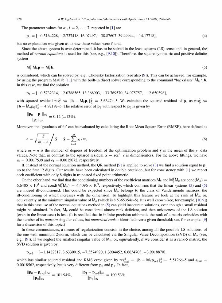
The parameter values for αi , i = 2, . . . , 7, reported in [1] are

p0 = [−0.5164228, −2.737418, 16.07497, −38.87607, 39.49944, −14.17718], (4)

but no explanation was given as to how these values were found.Since the above system is over-determined, it has to be solved in the least squares (LS) sense and, in general, the

method of normal equations is used for this (see, e.g., [9,10]). Therefore, the square symmetric and positive definitesystem

MTb Mbp = MT

b b, (5)

is considered, which can be solved by, e.g., Cholesky factorization (see also [9]). This can be achieved, for example,by using the program Matlab [11] with the built-in direct solver corresponding to the command “backslash” Mb \ b.In this case, we find the solution

p1 = [−0.5732314, −2.0788565, 13.368903, −33.769570, 34.975757, −12.650398],

with squared residual res21 := ‖b − Mbp1‖

22 = 3.6347e–5. We calculate the squared residual of p0 as res2

0 :=

‖b − Mbp0‖22 = 4.9219e–5. The relative error of p1 with respect to p0 is given by

‖p0 − p1‖∞

‖p0‖∞

= 0.12 (≡12%).

Moreover, the ‘goodness of fit’ can be evaluated by calculating the Root Mean Square Error (RMSE), here defined as

ε =

√S

m − n

/y, y =

m∑i=1

yi/m, (6)

where m − n is the number of degrees of freedom of the optimization problem and y is the mean of the yi datavalues. Note that, in contrast to the squared residual S ≡ res2, ε is dimensionless. For the above fittings, we haveε0 = 0.0017539 and ε1 = 0.0015072, respectively.

If, instead of the normal equation method, the QR method [9] is applied to solve (3) we find a solution equal to p1up to the first 12 digits. Our results have been calculated in double precision, but for consistency with [1] we reporteach coefficient with only 8 digits in truncated fixed point arithmetic.

On the other hand, we find that the conditioning numbers of the coefficient matrices Mb and MTb Mb are cond(Mb) =

6.6405 × 104 and cond(MTb Mb) = 4.4096 × 109, respectively, which confirms that the linear systems (3) and (5)

are indeed ill-conditioned. This could be expected since Mb belongs to the class of Vandermonde matrices, theill-conditioning of which increases with the dimension. To highlight this feature we look at the rank of Mb, or,equivalently, at the minimum singular value of Mb (which is 8.5365354e–5). It is well known (see, for example, [10,9])that in this case use of the normal equations method in (5) can yield inaccurate solutions, even though a small residualmight be obtained. In fact, Mb could be considered almost rank deficient, and then uniqueness of the LS solution(even in the linear case) is lost. (It is recalled that in infinite precision arithmetic the rank of a matrix coincides withthe number of its nonzero singular values, but numerical rank is identified over a given threshold; see, for example, [9]for a discussion of this topic.)

In these circumstances, a means of regularization consists in the choice, among all the possible LS solutions, ofthe one with minimum 2-norm, which can be calculated via the Singular Value Decomposition (SVD) of Mb (see,e.g., [9]). If we neglect the smallest singular value of Mb, or, equivalently, if we consider it as a rank-5 matrix, theSVD solution is given by

psvd = [−1.1482317, 3.6330015, −7.3574920, 1.3904452, 6.6634703, −3.9018870],

which has similar squared residual and RMS error given by res2svd = ‖b − Mbpsvd‖

22 = 5.5126e–5 and εsvd =

0.0018562, respectively, but is very different from p0 and p1. In fact,

‖p0 − psvd‖∞

‖p0‖∞

= 101.94%,‖p1 − psvd‖∞

‖p1‖∞

= 100.53%.

R.W. Ogden et al. / Computers and Mathematics with Applications 53 (2007) 276–286 279

Fig. 1. Left figure: interpolation curves AF7(z)/kBT (log scale) against z with the values p0, p1, psvd as coefficients of the polynomial in F7(z)in (2) compared with the synthetic data (circles). The three plots are indistinguishable. Right figure: corresponding relative errors with respect tothe synthetic data.

Note that ‖p0‖2 = 59.487072, ‖p1‖2 = 52.029778 and ‖psvd‖2 = 11.410947. The left-hand figure in Fig. 1 showsa logarithmic plot AF7(z)/kBT against z for each of the LS solutions p0, p1, psvd on the synthetic data (shown ascircles). The three curves are indistinguishable and the relative errors with respect to the synthetic data are all lessthan 1% and are reported in the right-hand figure in Fig. 1.

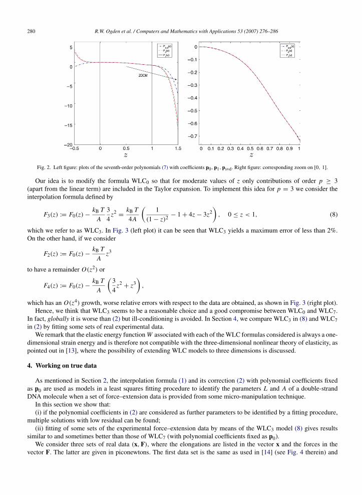
It is worth remarking that seventh-order polynomials, defined by

Pk(z) =

7∑i=2

α(k)i zi , k ∈ {0, 1, svd} , (7)

with coefficients given by the values in p0, p1 and psvd, respectively, are almost coincident on the interval [0, 1], onwhich (2) is always evaluated (see Fig. 2). For example, for z ∈ [0, 1], we have

‖P0(z) − Psvd(z)‖∞

‖P0(z)‖∞

' 1.59%,‖P1(z) − Psvd(z)‖∞

‖P1(z)‖∞

' 0.89%

and the polynomials only differ near z = 1.In any case care is needed since the difference between the predictions of two such polynomials may be emphasized

when the first and second derivatives of these models are considered, as may be appreciated by a simple computation.

3. A new interpolation formula

As reported in Section 1, the main drawback with the model (1) is the relatively poor data prediction for moderateextensions. As noted in [2,12], the expansion of (1) for small values of z = x/L gives

F0(z) ≈3kB T

2Az,

and then the double-strand DNA behaves like a linear spring with Hooke’s constant equal to kDNA = 3kBT/(2AL).Indeed, Taylor expansion of (1) around z = 0 gives

F0(z) =kB T

A

(32

z +34

z2+ z3

+54

z4+

32

z5+ O(z6)

),

and then for moderate elongations (z ≤ 0.5) quadratic contributions become too significant with respect to the smalldata values of the applied force.

280 R.W. Ogden et al. / Computers and Mathematics with Applications 53 (2007) 276–286

Fig. 2. Left figure: plots of the seventh-order polynomials (7) with coefficients p0, p1, psvd. Right figure: corresponding zoom on [0, 1].

Our idea is to modify the formula WLC0 so that for moderate values of z only contributions of order p ≥ 3(apart from the linear term) are included in the Taylor expansion. To implement this idea for p = 3 we consider theinterpolation formula defined by

F3(z) := F0(z) −kB T

A34

z2=

kB T4A

(1

(1 − z)2 − 1 + 4z − 3z2)

, 0 ≤ z < 1, (8)

which we refer to as WLC3. In Fig. 3 (left plot) it can be seen that WLC3 yields a maximum error of less than 2%.On the other hand, if we consider

F2(z) := F0(z) −kB T

Az3

to have a remainder O(z2) or

F4(z) := F0(z) −kB T

A

(34

z2+ z3

),

which has an O(z4) growth, worse relative errors with respect to the data are obtained, as shown in Fig. 3 (right plot).Hence, we think that WLC3 seems to be a reasonable choice and a good compromise between WLC0 and WLC7.

In fact, globally it is worse than (2) but ill-conditioning is avoided. In Section 4, we compare WLC3 in (8) and WLC7in (2) by fitting some sets of real experimental data.

We remark that the elastic energy function W associated with each of the WLC formulas considered is always a one-dimensional strain energy and is therefore not compatible with the three-dimensional nonlinear theory of elasticity, aspointed out in [13], where the possibility of extending WLC models to three dimensions is discussed.

4. Working on true data

As mentioned in Section 2, the interpolation formula (1) and its correction (2) with polynomial coefficients fixedas p0 are used as models in a least squares fitting procedure to identify the parameters L and A of a double-strandDNA molecule when a set of force–extension data is provided from some micro-manipulation technique.

In this section we show that:(i) if the polynomial coefficients in (2) are considered as further parameters to be identified by a fitting procedure,

multiple solutions with low residual can be found;(ii) fitting of some sets of the experimental force–extension data by means of the WLC3 model (8) gives results

similar to and sometimes better than those of WLC7 (with polynomial coefficients fixed as p0).We consider three sets of real data (x, F), where the elongations are listed in the vector x and the forces in the

vector F. The latter are given in piconewtons. The first data set is the same as used in [14] (see Fig. 4 therein) and

R.W. Ogden et al. / Computers and Mathematics with Applications 53 (2007) 276–286 281

Fig. 3. Left figure: relative errors with respect to synthetic data for F0(z), F7(z) and F3(z) (log scale). The horizontal line is at the 2% level. Rightfigure: relative errors on synthetic data for the interpolation formulas F0(z), F2(z), F3(z), F4(z).

labelled (B), with the x values given in nanometers (nm). The second set, labelled (C), has been considered in [15] andconcerns single-strand DNA experiments; in this case the elongations x are normalized by the contour length of theequivalent double-strand molecule. Both sets have also been used recently in [16] to test a new interpolation formulafor semi-flexible polymers. The third data set, labelled (F), has been obtained in the experiments of Renaud Fulconisand Jean-Louis Viovy (Institute Curie, Paris). The x values are given in microns (µm).

The nonlinear least squares (NLS) fitting algorithm used in this section is based on the lsqcurvefit.m routine inMatlab [11], and the Trust Region Method has been selected to solve the problem minp F(p), where the squaredtwo-norm of residues is defined by

F(p) ≡

m∑i=1

[F(p, xi ) − Fi ]2,

(xi , Fi ), i = 1, . . . , m, are the data points, p represents the vector of parameters and F(p, xi ) is chosen asF0(x/L), F7(x/L) and F3(x/L) in (1), (2) and (8), respectively. If p∗ is the optimum set of parameters obtainedby the above fitting procedure the corresponding squared residual is res2

= F(p∗) and the relative errors are definedby

erri :=|F(p∗, xi ) − Fi |

|Fi |, i = 1, . . . , m.

In the following we will also report the RMSE ε in (6) to estimate the goodness of each fit.

4.1. Case 1: Multiple LS solutions

To highlight the point concerning non-uniqueness of the parameters in WLC7, first of all we consider the syntheticdata (z, y) from [1]. The parameters to be identified in the model F7(z) in (2) are then p = [α2, . . . , α7] andµ0 = kBT/A.

We find two different sets of parameters that describe the data very well such that the curves are not distinguishable(as shown in Fig. 4). The same value of µ0, namely 0.9999, is obtained in each case, while one set of constants p isgiven by

p(1)= [−0.5494, −0.1213, −0.5269, 0.0320, 0.2061, 0.2930]

and the second set by

p(2)= [−0.6589, 0.5516, −1.7188, 0.2246, 1.3643, −0.4372].

282 R.W. Ogden et al. / Computers and Mathematics with Applications 53 (2007) 276–286

Fig. 4. Logarithmic plots (indistinguishable) of F7(z) against extension based on fitting of (2) to the WLC synthetic data (circles) with two(different) sets of material constants.

The two sets are significantly different, but the squared residual is very small in each case, respectively 1.2433e–4 and9.3811e–5 for the first and second sets. The corresponding RMS errors are 0.002879 and 0.00250081, respectively.We now show that this non-uniqueness is also found when working with real experimental data sets.

Let us consider the data set (F), obtained at temperature T = 298 K. The parameters to be identified in WLC7in (2) are now α = [α2, . . . , α7], A and L . Units used to represent the fitting results are nanometers (nm) for A, andmicrons (µm) for L (in fact in the calculations we identify Am = A/kB in K/pN). We solve the numerical fittingproblem by choosing as a starting guess for p = α the set p0 in (4) and for the persistence and contour lengths thevalues A = 38 nm and L = 4.4 µm (private communication from S. Neukirch). We find the following LS solution,referred as set (1):

A(1)= 23.498118 nm, L(1)

= 5.6565231 µm,

α(1)= [−19.9300, 217.66547, −1135.7121, 3081.2914, −4208.1388, 2323.5313],

with squared residual res2(1) = 0.0001370.

By considering two different randomly generated starting approximations, we find another two sets of parameters,say set (2) and set (3), with similar squared residuals, namely

A(2)= 38.281798 nm, L(2)

= 5.5388558 µm,

α(2)= [−16.543481, 246.82266, −1435.7216, 4091.6002, −5696.1681, 3161.5977],

with squared residual res2(2) = 0.0001353, and

A(3)= 308 nm, L(3)

= 4.8232480 µm,

α(3)= [60.062706, 267.05858, −3179.7139, 10 482.225, −14 724.507, 7847.2394],

with res2(3) = 0.0001362. Note that for this data set, since also the polynomial coefficients have to be identified, the

number of degrees of freedom is m − n = −1 and (6) is not properly defined. To also give in this case a measure ofthe ‘goodness of fit’, only for this example, we decided to report the RMS errors calculated by considering |m − n| inthe denominator of (6). With this choice, we have ε(1)

= 0.011705, ε(2)= 0.011632, ε(3)

= 0.01167.If in (2) we fix the polynomial coefficients as α ≡ p0 in (4), then the parameters identified are A(4)

=

33.790475 nm, L(4)= 4.5336477 µm with the larger squared residual res2

(4) = 0.00232881 (see Table 2 in thenext section for more details). In this case n = 2 and the RMS error according to the original formula (6) isε(4)

= 0.034123. We refer to this solution as set (4).Fig. 5 shows the fitting results for the above four sets of parameters, set (4) being identified by the symbol ‘+’.

The left figure shows the original data set (F). Note that the fitting curves in the right figure, that is the function Fk7 (z),

with k = 1, 2, 3, 4 corresponding to the sets (1), (2), (3), (4), are different partly because they correspond to different

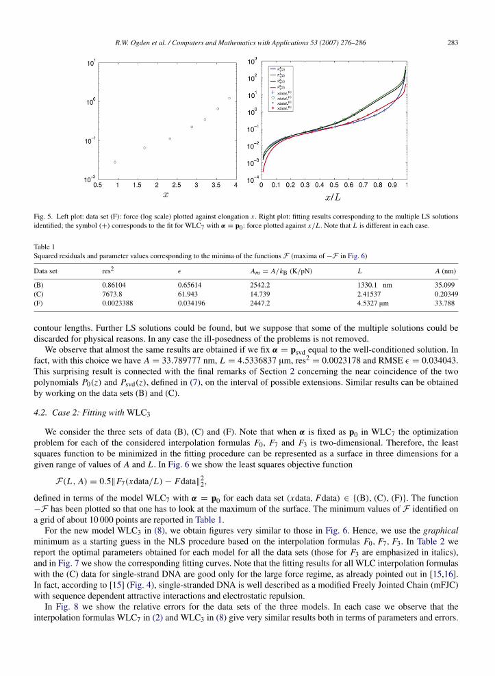
R.W. Ogden et al. / Computers and Mathematics with Applications 53 (2007) 276–286 283

Fig. 5. Left plot: data set (F): force (log scale) plotted against elongation x . Right plot: fitting results corresponding to the multiple LS solutionsidentified; the symbol (+) corresponds to the fit for WLC7 with α ≡ p0: force plotted against x/L . Note that L is different in each case.

Table 1Squared residuals and parameter values corresponding to the minima of the functions F (maxima of −F in Fig. 6)

Data set res2 ε Am = A/kB (K/pN) L A (nm)

(B) 0.86104 0.65614 2542.2 1330.1 nm 35.099(C) 7673.8 61.943 14.739 2.41537 0.20349(F) 0.0023388 0.034196 2447.2 4.5327 µm 33.788

contour lengths. Further LS solutions could be found, but we suppose that some of the multiple solutions could bediscarded for physical reasons. In any case the ill-posedness of the problems is not removed.

We observe that almost the same results are obtained if we fix α = psvd equal to the well-conditioned solution. Infact, with this choice we have A = 33.789777 nm, L = 4.5336837 µm, res2

= 0.0023178 and RMSE ε = 0.034043.This surprising result is connected with the final remarks of Section 2 concerning the near coincidence of the twopolynomials P0(z) and Psvd(z), defined in (7), on the interval of possible extensions. Similar results can be obtainedby working on the data sets (B) and (C).

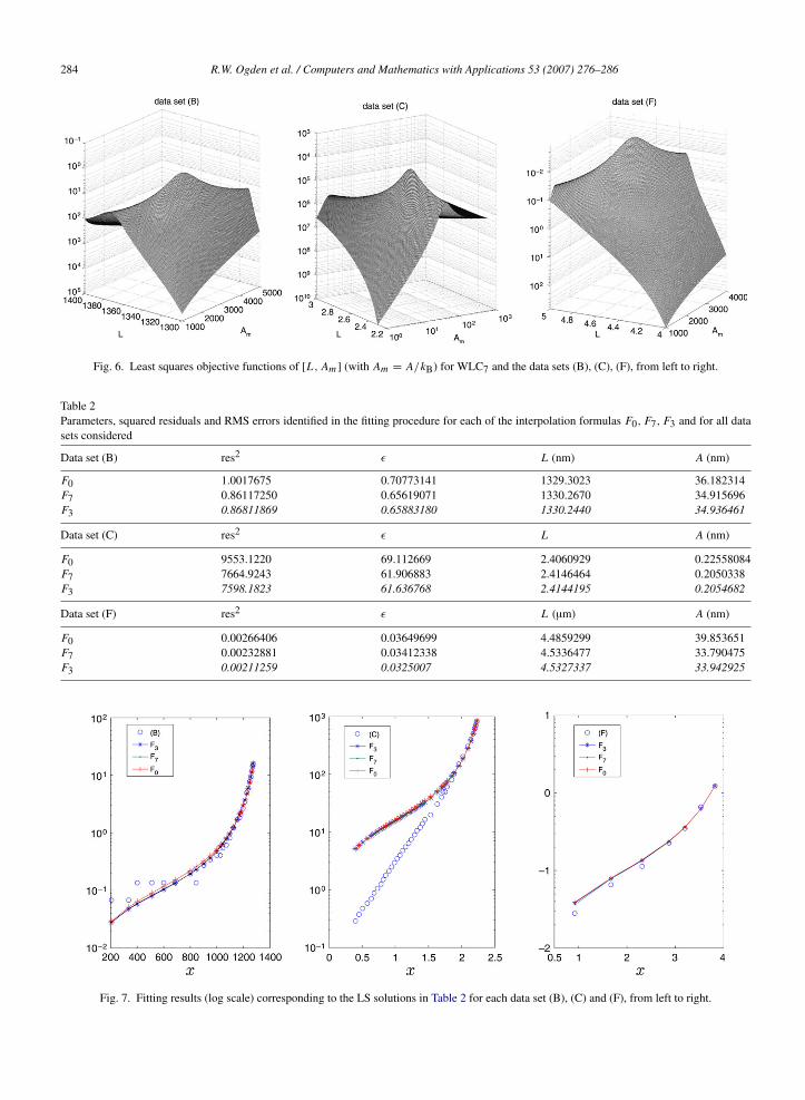
4.2. Case 2: Fitting with WLC3

We consider the three sets of data (B), (C) and (F). Note that when α is fixed as p0 in WLC7 the optimizationproblem for each of the considered interpolation formulas F0, F7 and F3 is two-dimensional. Therefore, the leastsquares function to be minimized in the fitting procedure can be represented as a surface in three dimensions for agiven range of values of A and L . In Fig. 6 we show the least squares objective function

F(L , A) = 0.5‖F7(xdata/L) − Fdata‖22,

defined in terms of the model WLC7 with α = p0 for each data set (xdata, Fdata) ∈ {(B), (C), (F)}. The function−F has been plotted so that one has to look at the maximum of the surface. The minimum values of F identified ona grid of about 10 000 points are reported in Table 1.

For the new model WLC3 in (8), we obtain figures very similar to those in Fig. 6. Hence, we use the graphicalminimum as a starting guess in the NLS procedure based on the interpolation formulas F0, F7, F3. In Table 2 wereport the optimal parameters obtained for each model for all the data sets (those for F3 are emphasized in italics),and in Fig. 7 we show the corresponding fitting curves. Note that the fitting results for all WLC interpolation formulaswith the (C) data for single-strand DNA are good only for the large force regime, as already pointed out in [15,16].In fact, according to [15] (Fig. 4), single-stranded DNA is well described as a modified Freely Jointed Chain (mFJC)with sequence dependent attractive interactions and electrostatic repulsion.

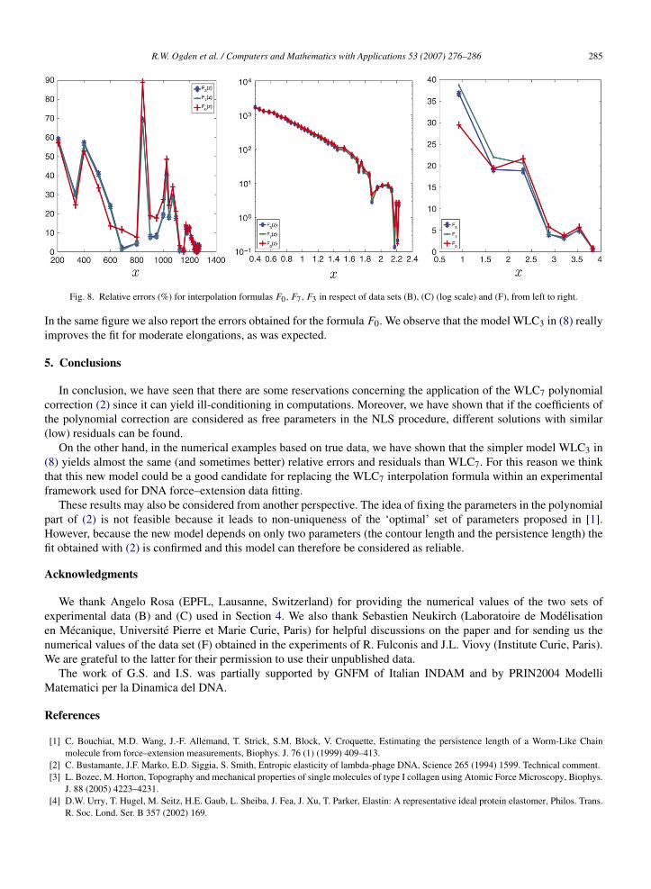
In Fig. 8 we show the relative errors for the data sets of the three models. In each case we observe that theinterpolation formulas WLC7 in (2) and WLC3 in (8) give very similar results both in terms of parameters and errors.

284 R.W. Ogden et al. / Computers and Mathematics with Applications 53 (2007) 276–286

Fig. 6. Least squares objective functions of [L , Am ] (with Am = A/kB) for WLC7 and the data sets (B), (C), (F), from left to right.

Table 2Parameters, squared residuals and RMS errors identified in the fitting procedure for each of the interpolation formulas F0, F7, F3 and for all datasets considered

Data set (B) res2 ε L (nm) A (nm)

F0 1.0017675 0.70773141 1329.3023 36.182314F7 0.86117250 0.65619071 1330.2670 34.915696F3 0.86811869 0.65883180 1330.2440 34.936461

Data set (C) res2 ε L A (nm)

F0 9553.1220 69.112669 2.4060929 0.22558084F7 7664.9243 61.906883 2.4146464 0.2050338F3 7598.1823 61.636768 2.4144195 0.2054682

Data set (F) res2 ε L (µm) A (nm)

F0 0.00266406 0.03649699 4.4859299 39.853651F7 0.00232881 0.03412338 4.5336477 33.790475F3 0.00211259 0.0325007 4.5327337 33.942925

Fig. 7. Fitting results (log scale) corresponding to the LS solutions in Table 2 for each data set (B), (C) and (F), from left to right.

R.W. Ogden et al. / Computers and Mathematics with Applications 53 (2007) 276–286 285

Fig. 8. Relative errors (%) for interpolation formulas F0, F7, F3 in respect of data sets (B), (C) (log scale) and (F), from left to right.

In the same figure we also report the errors obtained for the formula F0. We observe that the model WLC3 in (8) reallyimproves the fit for moderate elongations, as was expected.

5. Conclusions

In conclusion, we have seen that there are some reservations concerning the application of the WLC7 polynomialcorrection (2) since it can yield ill-conditioning in computations. Moreover, we have shown that if the coefficients ofthe polynomial correction are considered as free parameters in the NLS procedure, different solutions with similar(low) residuals can be found.

On the other hand, in the numerical examples based on true data, we have shown that the simpler model WLC3 in(8) yields almost the same (and sometimes better) relative errors and residuals than WLC7. For this reason we thinkthat this new model could be a good candidate for replacing the WLC7 interpolation formula within an experimentalframework used for DNA force–extension data fitting.

These results may also be considered from another perspective. The idea of fixing the parameters in the polynomialpart of (2) is not feasible because it leads to non-uniqueness of the ‘optimal’ set of parameters proposed in [1].However, because the new model depends on only two parameters (the contour length and the persistence length) thefit obtained with (2) is confirmed and this model can therefore be considered as reliable.

Acknowledgments

We thank Angelo Rosa (EPFL, Lausanne, Switzerland) for providing the numerical values of the two sets ofexperimental data (B) and (C) used in Section 4. We also thank Sebastien Neukirch (Laboratoire de Modelisationen Mecanique, Universite Pierre et Marie Curie, Paris) for helpful discussions on the paper and for sending us thenumerical values of the data set (F) obtained in the experiments of R. Fulconis and J.L. Viovy (Institute Curie, Paris).We are grateful to the latter for their permission to use their unpublished data.

The work of G.S. and I.S. was partially supported by GNFM of Italian INDAM and by PRIN2004 ModelliMatematici per la Dinamica del DNA.

References

[1] C. Bouchiat, M.D. Wang, J.-F. Allemand, T. Strick, S.M. Block, V. Croquette, Estimating the persistence length of a Worm-Like Chainmolecule from force–extension measurements, Biophys. J. 76 (1) (1999) 409–413.

[2] C. Bustamante, J.F. Marko, E.D. Siggia, S. Smith, Entropic elasticity of lambda-phage DNA, Science 265 (1994) 1599. Technical comment.[3] L. Bozec, M. Horton, Topography and mechanical properties of single molecules of type I collagen using Atomic Force Microscopy, Biophys.

J. 88 (2005) 4223–4231.[4] D.W. Urry, T. Hugel, M. Seitz, H.E. Gaub, L. Sheiba, J. Fea, J. Xu, T. Parker, Elastin: A representative ideal protein elastomer, Philos. Trans.

R. Soc. Lond. Ser. B 357 (2002) 169.

286 R.W. Ogden et al. / Computers and Mathematics with Applications 53 (2007) 276–286

[5] J.F. Marko, Coupling of intramolecular and intermolecular linkage complexity of two DNAs, Phys. Rev. E 59 (1999) 900–912.[6] J.F. Marko, E.D. Siggia, Statistical mechanics of supercoiled DNA, Phys. Rev. E 52 (1995) 2912–2938.[7] O. Kratky, G. Porod, Rontgenuntersuchung geloster Fadenmolekule, Recueil des Travaux Chimiques des Pays Bas - J. of the Royal

Netherlands Chem. Soc. 68 (1949) 1106–1123.[8] J.F. Marko, E.D. Siggia, Stretching DNA, Macromolecules 28 (1995) 8759–8770.[9] G.H. Golub, C.F. Van Loan, Matrix Computation, 3rd ed., Johns Hopkins University Press, Baltimore, London, 1996.

[10] A. Bjorck, Numerical Methods for Least Squares Problems, SIAM Press, Philadelphia, 1996.[11] MATLAB 6.5, Release 13, Optimisation Toolbox 2.2, Users Guide.[12] C. Bustamante, S.B. Smith, J. Liphardt, D. Smith, Single molecule studies of DNA mechanics, Curr. Opin. Struct. Biol. 10 (2000) 279–285.[13] R.W. Ogden, G. Saccomandi, I. Sgura, On Worm-Like Chain model within the three-dimensional continuum mechanics framework, Proc.

Roy. Soc. A 462 (2067) (2006) 749–768, doi:10.1098/rspa.2005.1592.[14] C.G. Baumann, V.A. Bloomfield, S.B. Smith, C. Bustamante, M.D. Wang, S.M. Block, Stretching of single collapsed DNA molecules,

Biophys. J. 78 (2000) 1965–1978.[15] M.-N. Dessinges, B. Maier, Y. Zhang, M. Peliti, D. Bensimon, V. Croquette, Stretching single stranded DNA, a model polyelectrolyte, Phys.

Rev. Lett. 89 (2002) 248102.[16] A. Rosa, T.X. Hoang, D. Marenduzzo, A. Maritan, A new interpolation formula for semiflexible polymers, Biophys. Chem. 115 (2005)

251–254.