
worm wheel
78
1. INTRODUCTION A worm drive is a gear arrangement in which a worm (which is a gear in the form of a screw) meshes with a worm gear (which is similar in appearance to a spur gear, and is also called a worm wheel). The terminology is often confused by imprecise use of the term worm gear to refer to the worm, the worm gear, or the worm drive as a unit. Like other gear arrangements, a worm drive can reduce rotational speed or allow higher torque to be transmitted. The image shows a section of a gear box with a worm gear being driven by a worm. A worm is an example of a screw, one of the six simple machines 1.1 Explanation of worm wheel: A gearbox designed using a worm and worm-wheel will be considerably smaller than one made from plain spur gears and has its drive axes at 90° to each other. With a single start worm, for each 360° turn of the worm, the worm-gear advances only one tooth of the gear. Therefore, regardless of the worm's size (sensible engineering limits notwithstanding), the gear ratio is the "size of the worm gear - to - 1". Given a single start worm, a 20 tooth worm gear will reduce the speed by the ratio of 20:1. With spur gears, a gear of 12 teeth (the smallest size permissible, if designed to good engineering practices) would have to be matched with a 240 tooth gear to achieve the same ratio of 20:1. Therefore, if the diametrical pitch (DP) of each gear was the same, then, in terms of the physical size of the 240 tooth gear to that of the 20 tooth gear, the worm arrangement is considerably smaller in volume.
Transcript of worm wheel

1. INTRODUCTION
A worm drive is a gear arrangement in which a worm (which is a
gear in the form of a screw) meshes with a worm gear (which is
similar in appearance to a spur gear, and is also called a
worm wheel). The terminology is often confused by imprecise
use of the term worm gear to refer to the worm, the worm gear,
or the worm drive as a unit.
Like other gear arrangements, a worm drive can reduce
rotational speed or allow higher torque to be transmitted. The
image shows a section of a gear box with a worm gear being
driven by a worm. A worm is an example of a screw, one of the
six simple machines
1.1 Explanation of worm wheel:
A gearbox designed using a worm and worm-wheel will be
considerably smaller than one made from plain spur gears and
has its drive axes at 90° to each other. With a single start worm,
for each 360° turn of the worm, the worm-gear advances only
one tooth of the gear. Therefore, regardless of the worm's
size (sensible engineering limits notwithstanding), the gear
ratio is the "size of the worm gear - to - 1". Given a single start
worm, a 20 tooth worm gear will reduce the speed by the ratio
of 20:1. With spur gears, a gear of 12 teeth (the smallest
size permissible, if designed to good engineering practices)
would have to be matched with a 240 tooth gear to achieve the
same ratio of 20:1. Therefore, if the diametrical pitch (DP)
of each gear was the same, then, in terms of the physical size
of the 240 tooth gear to that of the 20 tooth gear, the worm
arrangement is considerably smaller in volume.

1.2 Types of worm wheel:
There are three different types of gears that can be used in a
worm drive.
The first are non-throated worm gears. These don't have a throat,
or groove, machined around the circumference of either the
worm or worm wheel. The second are single-throated worm gears,
in which the worm wheel is throated. The final type are
double-throated worm gears, which have both gears throated.
This type of gearing can support the highest loading.
An enveloping (hourglass) worm has one or more teeth and
increases in diameter from its middle portion toward both
ends. Double-enveloping wormgearing comprises enveloping worms
mated with fully enveloping wormgears. It is also known as
globoidal wormgearing.
-01-
1.3 Direction of transmission
Unlike with ordinary gear trains, the direction of
transmission (input shaft vs output shaft) is not reversible
when using large reduction ratios, due to the greater friction
involved between the worm and worm-wheel, when usually a
single start (one spiral) worm is used. This can be an
advantage when it is desired to eliminate any possibility of
the output driving the input. If a multistart worm (multiple
spirals) is used then the ratio reduces accordingly and the
braking effect of a worm and worm-gear may need to be discounted
as the gear may be able to drive the worm.

Worm gear configurations in which the gear cannot drive the
worm are said to be self-locking. Whether a worm and gear will be
self-locking depends on the lead angle, the pressure angle,
and the coefficient of friction; however, it is approximately
correct to say that a worm and gear will be self-locking if
the tangent of the lead angle is less than the coefficient of
friction.
1.4 Applications of worm wheel:
In early 20th century automobiles prior to the introduction of
power steering, the effect of a flat or blowout on one of the
front wheels will tend to pull the steering mechanism toward
the side with the flat tire. The employment of a worm screw
reduced this effect. Further development of the worm drive
employs recirculating ball bearings to reduce frictional
forces, allowing some of the steering force to be felt in the
wheel as an aid to vehicle control and greatly reducing wear,
which leads to difficulties in steering precisely.
Worm drives are a compact means of substantially decreasing
speed and increasing torque. Small electric motors are
generally high-speed and low-torque; the addition of a worm
drive increases the range of applications that it may be
suitable for, especially when the worm drive's compactness is
considered.
Worm drives are used in presses, rolling mills, conveying
engineering, mining industry machines, on rudders, and worm
drive saws. In addition, milling heads and rotary tables are
positioned using high-precision duplex worm drives with
adjustable backlash. Worm gears are used on many lift/elevator

and escalator-drive applications due to their compact size and
the non-reversibility of the gear.
-02-
In the era of sailing ships, the introduction of a worm drive
to control the rudder was a significant advance. Prior to its
introduction, a rope drum drive was used to control the
rudder, and rough seas could cause substantial force to be
applied to the rudder, often requiring several men to steer
the vessel, with some drives having two large-diameter wheels
to allow up to four crewmen to operate the rudder.
Figure:1 Truck final drive of the 1930s
Worm drives have been used in a few automotive rear-axle final
drives (although not the differential itself at this time).
They took advantage of the location of the gear being at
either the very top or very bottom of the differential crown
wheel. In the 1910s they were common on trucks; to gain the
most clearance on muddy roads the worm gear was placed on top.
In the 1920s the Stutz firm used them on its cars; to have a
lower floor than its competitors, the gear was located on the
bottom. An example from around 1960 was the Peugeot 404. The
worm gear carries the differential gearing, which protects the

vehicle against rollback. This ability has largely fallen from
favour due to the higher-than-necessary reduction ratios.
A more recent exception to this is the Torsen differential,
which uses worms and planetary worm gears in place of the
bevel gearing of conventional open differentials. Torsen
differentials are most prominently featured in the HMMWV and
some commercial Hummer vehicles, and as a center differential
in some all wheel drive systems, such as Audi's quattro. Very
heavy trucks, such as those used to carry aggregates, often
use a worm gear differential for strength. The worm drive is
not as efficient as a hypoid gear, and such trucks invariably
have a very large differential housing, with a correspondingly
large volume of gear oil, to absorb and dissipate the heat
created.
-03-
Worm drives are used as the tuning mechanism for many musical
instruments, including guitars, double-basses, mandolins,
bouzoukis, and many banjos (although most high-end banjos use
planetary gears or friction pegs). A worm drive tuning device
is called a machine head.
Plastic worm drives are often used on small battery-operated
electric motors, to provide an output with a lower angular
velocity (fewer revolutions per minute) than that of the
motor, which operates best at a fairly high speed. This motor-
worm-gear drive system is often used in toys and other small
electrical devices.
A worm drive is used on jubilee-type hose clamps or jubilee
clamps; the tightening screw has a worm thread which engages
with the slots on the clamp band.
Occasionally a worm gear is designed to be run in reverse,
resulting in the output shaft turning much faster than the
input. Examples of this may be seen in some hand-cranked
centrifuges or the wind governor in a musical box.
1.5 Left hand and right hand worm:
A right hand helical gear or right hand worm is one in which
the teeth twist clockwise as they recede from an observer
looking along the axis. The designations, right hand and left
hand, are the same as in the long established practice for
screw threads, both external and internal. Two external
helical gears operating on parallel axes must be of opposite
hand. An internal helical gear and its pinion must be of the
same hand.
-04-

A left hand helical gear or left hand worm is one in which the
teeth twist counter clockwise as they recede from an observer
looking along the axis.
Figure:2 Left hand and right hand of helical gear and worm

-05-
2. LITERATURE SURVEY:
Walker gives a short summary of the origins and the initial
development of worm gears. Archimedes is credited with
introducing the worm gear concept by interlocking a screw,
thread and toothed wheel. An improvement made by cutting a
radius into the tip of the wheel tooth to allow for the worm
thread root diameter was termed a single enveloping gear set. The
clearance allowed a smaller centre distance as the wheel
begins to envelop the worm. Loveless reports that Leonardo
DaVinci developed the double enveloping gear set concept in the 15th
century by varying the worm thread height relative to a radius
about the wheel axis. However, in the same paper Henry Hindley
is largely credited as the first to manufacture gear sets of
this type in the 18thcentury. The reduction in centre
distances provided a more compact system and increased the
length of worm thread flank making contact with the wheel
teeth. This combination resulted in a smaller unit being able
to transmit a higher torque load theoretically.
Vos identifies the CAVEX form as originally developed by
Flender in the early 1950's. This type of worm drive derives
its name from the concave flanks of the worm thread which
differed from conventional convex forms. This improved the
theoretical efficiency and the potential load capacity
relative to an equivalent single enveloping system by

directing more of the force parallel to the worm axis, and
consequently tangential to the wheel rotation.
No scientific basis was defined for worm gear development
until approximately the 1920's. At this point, research into
various design principles for cylindrical worm gear sets was
recorded by Tuplin and Merritt. Work by Merritt and Walker led
to the standardisation of gear production through the initial
development of BS721 in the 1930's. This standard had a latest
revision in 1983 and is still used by industrial gear
designers today to determine the worm and wheel tooth
dimensions.
Analysis of worm gear contact initially involved modelling
worm thread flanks as a series of helices about an axis. These
helices passed through a profile which was determined by the
worm gear type. A detailed analysis for cylindrical gear forms
soon followed from Buckingham in which standard equations were
defined. This derived equations for the geometry of involute,
screw, chased, and milled helicoids worm forms. The analysis
goes on to calculate the 3-dimensional co-ordinates of
theoretical contact lines for the engaging flanks, and
pressure angles relating to the curvature of the thread
profiles which determine
-06-
the line of acting force. Authors such as Dudley and Poritslcy
also made considerable contributions in this area. From these
basic equations it has been possible to develop formulae for
the load capacity, stress limits, and efficiency of a gear
set.

A recent paper from Octrue showed that calculations of load
capacity using these fundamental equations gave a good
correlation with experimental results. This demonstrates the
importance and applicability of such equations to the
operating performance of worm gears.

-07-
2.1 Geometry and nomenclature:
Figure:3 Nomenclature of a single enveloping worm gear
a. The geometry of a worm is similar to that of a power screw.
Rotation of the worm
simulates a linearly advancing involute rack,
b. The geometry of a worm gear is similar to that of a helical
gear, except that the
teeth are curved to envelop the worm.
c. Enveloping the gear gives a greater area of contact but
requires extremely
precise mounting.

1. As with a spur or helical gear, the pitch diameter of a
worm gear is related to its
circular pitch and number of teeth Z by the formula
d Z pπ
-08-
2. When the angle is 90 between the nonintersecting shafts,
the worm lead angle
is equal to the gear helix angle. Angles and have the
same hand.
3. The pitch diameter of a worm is not a function of its
number of threads, Z1.
4. This means that the velocity ratio of a worm gear set is
determined by the ratio of
gear teeth to worm threads; it is not equal to the ratio of
gear and worm
diameters.
ω = Z
ω Z
5. Worm gears usually have at least 24 teeth, and the number
of gear teeth plus
worm threads should be more than 40:
Z1 + Z2 > 40

6. A worm of any pitch diameter can be made with any number of
threads and any
axial pitch.
7. For maximum power transmitting capacity, the pitch diameter
of the worm should
normally be related to the shaft center distance by the
following equation
C0.875 C0.875 in Machine Design II Prof. K.Gopinath & Prof.
M.M.Mayuram
Indian Institute of Technology Madras
8. Integral worms cut directly on the shaft can, of course,
have a smaller diameter
than that of shell worms, which are made separately.
9. Shell worms are bored to slip over the shaft and are driven
by splines, key, or
pin.
-09-
10. Strength considerations seldom permit a shell worm to have
a pitch diameter less
than
d1 = 2.4p + 1.1
11. The face width of the gear should not exceed half the worm
outside diameter.

b ≤ 0.5 da
12. Lead angle λ, Lead L, and worm pitch diameter d1 have the
following relationship
in connection with the screw threads.
tan λ= L (πd)
13. To avoid interference, pressure angles are commonly
related to the worm lead.
-10-
3.0 DESIGN OF WORM GEARING:

Selection Of Gear Box Parameters are given below;
At standared dimensional of worm gearing i=40
FOR i=40 ….from handbook of gear design
i m Z1 dw Γ c
40 5
mm
1 50 5.7106° 125
mm
dg = mzg = 5×40 = 200 mm
3.1 Calculation of output shaft revolutions:
ng= 1500/40 = 37.5 rpm
calculation of input shaft torque is given below;
T1 = H1w = H*30/Лn=150000/4712.38=31.83N.m
1.4 Some Important relations:-
αn=20°
αa =20.09°
3.2 Calculation of worm efficiency:
VW = πXdWXNW
60X1000

= π∗50∗150060∗1000 = 3.927m/s
-11-
Vs = Vw
cosλ
= = 3.947m/s
From Hand Book of Gear Design:-
Form fig . ( 14- 7 ) ……………………… μ = 0.028
η =
= =0.90=90%
3.3 Calculation of output shaft torque:
Tout = T2 = Ti . η .i LET η = 1
= 31.83* 40=1273.24N.m
3.4 Check of power rating:
For Centrefugal- cast bronze ks = 1000
for i = 40………k m = 0.815 … table ( - )
3.927
cos 5 .7
106
Cosα n-µtanγ
Cosαn-µtanγ
Cos 20-0.028tan5.7106
Cos 20+0.028tan
5.7106

for Vs =3.95.….k v 0.285 …table ( - )
fe= ⅔ dw = ⅔ x 50 = 33.3mm or fe=30 less
W G = β.K V. K S. K M. d G 0.8 . fe
-12-
= 0.0131* 1000(200)0.8 *30*0. 815 *0.285
W G = 6327.3N
WF =
=
= 294.692 N
HL=Wf*Vs=294.692*3.95=1164.03343W
Vgt=π ngdg/60=0.9m/s
HO =Wgt*Vgt=6327.3*0.9=5694.57W
H=Ho+Hl=1164.033+5694.57= 6858.6W>5000
3.5 Design of worm:
d a = dw + 2 m = 50+ 2 * 5= 60 mmd d = dw – 2.5 m = 50 - 2.5 * 5 =37.5 mm
3.6 Design of worm wheel:
d g = m x zg = 5 * 40 =200 mm
μ XWw
cos αn. sin λ + μ cos
λ cos T.028* 1273.24
cos 20 . sin 5.7106+..028cos 5.7106

d a = dg + 2m =200 + 2* 5 = 210 mm
d d = dg – 2.5 m = 200 - 2.5 * 5 = 187.5mm
-13-
4. INTRODUCTION OF CATIA:
CATIA V5 R18 (Computer Aided Three Dimensional Interactive
Application)
As the world’s one of the supplier of software,
specifically intended to support a totally Integrated product
development process. Dassault Systems (DDS) in recognized as a
strategic partner which can help a manufacturer to the turn a
process into competitive advance, greater market share and
higher profits and industrial and mechanical design to
functional simulation manufacturing and information
management.
Catia Mechanical design solution will improve our design
productivity. Catia is a suit of programs that are used in
design, analysis and manufacturing of a virually unlimited
range of the product.
“ Feature based” means that we create parts and
assemblies by defining feature like extrusion sweeps, cuts,
holes, round and so on instead of specifying low level
geometry like lines, areas circles. This means that the
designer can think of the computer model at a very high level
and leave all low geometry detail for Catia to figure out.

“Parametric” means that the physical shape of the part as
assembly is driven by the value assigned to the attributes of
its features. We may define or modify a feature dimension or
other attributes at any times. Any changes will automatically
propagate through the model.
“Solid Modeling “ means that the computer model we create
is able to contain all the information that a real solid
object would have. It has volumes and therefore, if you
provide a value for the density of the material it has mass
and inertia.
4.1 Benefits of CATIA:
1. It is much faster and more accurate than any CAD
system.
2. Once design is complete, 2-D and 3-D views are
readily obtainable.
3. The ability to change in late design process is
possible.
4. It provides a very accurate representation of model
specifying all the other dimensions hidden geometry
etc.
-14-
5. It provides a greater flexibility for change, for
example, if we like to change the dimensions in
design assembly, manufacturing etc. will
automatically change.

6. It provides clear 3-D Model which are easy to
visualize or model created and & it Also decrease
the time required for the assembly to a large
extent.
4.2 Applications of CATIA:
Feature and Capabilities
Commonly referred as a 3D product lifecycle
management software suite. CATA support multiple stages of
product development (CAx). The stages range from
conceptualization, through design (CAD) and manufacturing
(CAM) until analysis (CAE), as of 2007 the latest release is
V5 release 18(V5R 18)
4.2.1 Industries using CATIA:
CATIA is widely used through the engineering industry,
especially in the automotive and aerospace sectors, CATIA V4,
VATIA V5 are the dominant systems.
4.2.2. Aerospace:
The Boeing Company used CATIA to develop its 777
airliner, and is currently using CATIA V5 for the 787 series
aircraft. European aerospace giant airbus has been using CATIA
since 2001. In 2006 airbus announced that the reduction of it
airbus 380 using catia. Canadian aircraft maker bombardier
aerospace has done all if its designing on catia.
4.2.3. Automotive:
Automotive Companies that use CATOA to varying degrees
are BMW. Porsche, Daimler, Chrysler, Audi, Volvo, fiat,

Gestamp Automaocian, benteler AG PSA, Pevgcot Citroen,
Penault, Toyota, Honda, ford Scania, Hyundai proton (company),
TATA motors and Mahindra Goodyear uses it in making tires for
automotive and aerospace and also uses a customized CATIA for
its design and development. All automotive companies sue
CATIA for car structures door beams IP supports, bumber beams
root rails, side rails, body components because CATIA is very
good in surface creation and computer representation of
surfaces.
-15-
4.2.4. Ship building:
Dassault system has begun serving shipbuilders with CATIA
V5 release 8. which includes special features useful to
shipbuilders, GD Electric boat used CATIA to design the latest
fast attack submarine class for the united states Navy, the
virgina class, Northrop Grumman Newport news also used CATIA
to design the Gerald R.Ford class of supper carries for us
navy.
4.2.5. Future Implementation:
Dassualt system has announced plans to release CATIA
version 6 (V6) in mid 2008. the new interface allows designer
to work directly with the 3D solid model rather than the
feature based design approach employed in CATIA V5. This
version will also improve the product life cycle management in
a revolutionary way. This concept is called PLm.2. (in
reference of the so called revolution in the internet called
web 2.0)

4.3. Applications of CATIA in modeling:
CATIA Mechanical design solutions offer a modeler a
robust supporting unlimited geometric complex ability and
advanced surfacing capabilities ensuring an accurate
representation of our design.
CATIA automatically embeds design intent into models
providing the flexibility to optimized designs easily and
effectively, as we need.
CATIA offers intelligent product modeling consisting of
familiar parametric features that react predictably to any
change. This enables rapid alternatives all in a logical
engineering environment.
Full associatively guaranties the propagations of design
changes automatically throughout the entire system providing
the update deliverables such as assemblies, drawing, finite
element models, mould process plans and complete manufacturing
data.
CATIA total product representation enables part to part
modeling by capturing all engineering data throughout the
development process, allowing us to fully visualize accurate
product moulds, as they will appear when manufacture.
-16-
4.4 Geometric modeling:

There are number of applications of the CAD software, one
of the most popular applications being geometric modeling.
First of all let us see what is geometric modeling? The
computer compatible mathematical description of the geometric
of this is called as geometric modeling. The CAD software
allows the mathematical description of the object to be
displayed as the image on the monitor of the computer.
4.4.1 Steps for creating the geometric model:
There are three steps in which the designer can create
geometric models by using CAD software, these are:
Creation of basis geometric objects: in the steps the
designer creates basic geometric elements by suing
commands like points, lines and circles.
Transformations of the elements: In the second step the
designer uses commands like achieve scaling, rotation and
other related transformation of the geometric elements.
Creation of the geometric model: During the final step the
designer uses various commands to that cause integration of
the objects or elements of the geometric model to form the
desired shape.
During the process of geometric modeling the computer
converts various commands given from within the CAD software
into mathematical models, stores them as the files; and
finally displays them as the image. The geometric models
created by the designer can open at any time for reviewing,
editing or analysis.
4.4.2. Representation of the geometric models:

Of the various forms of representing the objects in
geometric models, the most basic is wire frames. In this form
the object is displayed by interconnected lines as shown in
the figure below. There are three types of wire frame
geometric modeling, these are: 2D, 2.1/2D and 3D. They have
been described below:
2D: It is stands of two dimensional view and is useful
for flat objects.
2.1/2D: It gives views beyond the 2D view and permits
viewing of 3D object
Ffthat has no sidewall details.
-17-
3D: The three dimension representation allows complete
three-dimensional viewing
Of the model with highly complex geometry. Solid
modeling is the most advanced method of geometric
modeling in three dimensions.
4.5 CATIA user interface:
Below is the layout of the elements of the standard CATIA
application.
A. Menu Commands
B. Specification Tree
C. Window of Active document
D. Filename and extension of current document

E. Icons to maximize/minimize and close window
F. Icon of the active workbench
G. Toolbars specific to the active workbench
H. Standard toolbar
I. Compass
J. Geometry
-18-
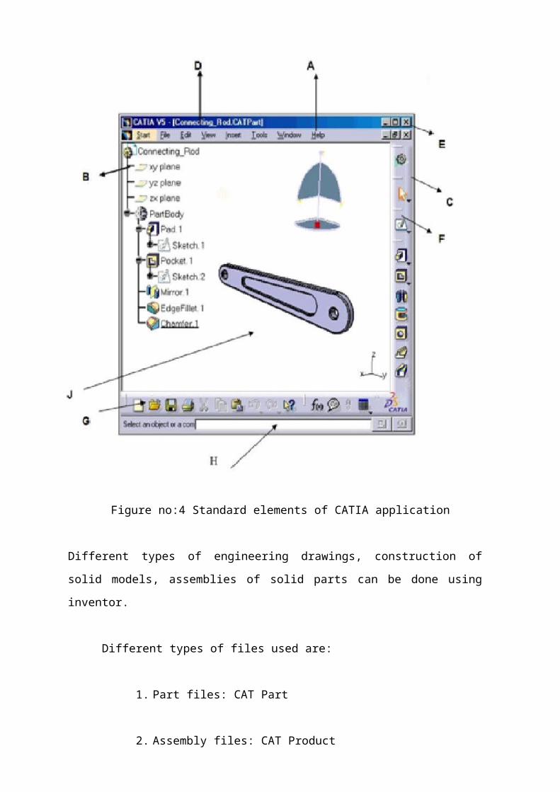
Figure no:4 Standard elements of CATIA application
Different types of engineering drawings, construction of
solid models, assemblies of solid parts can be done using
inventor.
Different types of files used are:
1. Part files: CAT Part
2. Assembly files: CAT Product

-19-
4.5.1 Work benches:
Workbenches contain various tools that you may need to
access during your part creation. You can switch between
any primary workbenches using the following two ways:
Figure no:5 Work benches
A. Use the Start Menu.
B. Click File >New to create a new document with a
particular file type. The associated workbench

automatically launches.
The parts of the major assembly is treated as individual
geometric model , which is modeled individually in separate
file .All the parts are previously planned & generated feature
by feature to construct full model.
-20-
Generally all CAD models are generated in the same passion
given bellow :
: Enter CAD
environment by clicking, later into part
designing
mode to construct model.
: Select plane as
basic reference.
: Enter sketcher
mode.
In sketcher mode:
: Tool used to create 2-d basic
structure of part using line, circle etc

: Tool used
for editing of created geometry termed
as
operation
: Tool used for
Dimensioning, referencing.
This helps creating
parametric relation.
: Its external feature to view
geometry in & out
: Tool used to exit sketcher mode after creating
geometry.
Sketch Based Feature:
Pad : On exit of sketcher mode the feature is to
be padded .( adding
material )
-21-
Pocket: On creation of basic structure
further pocket
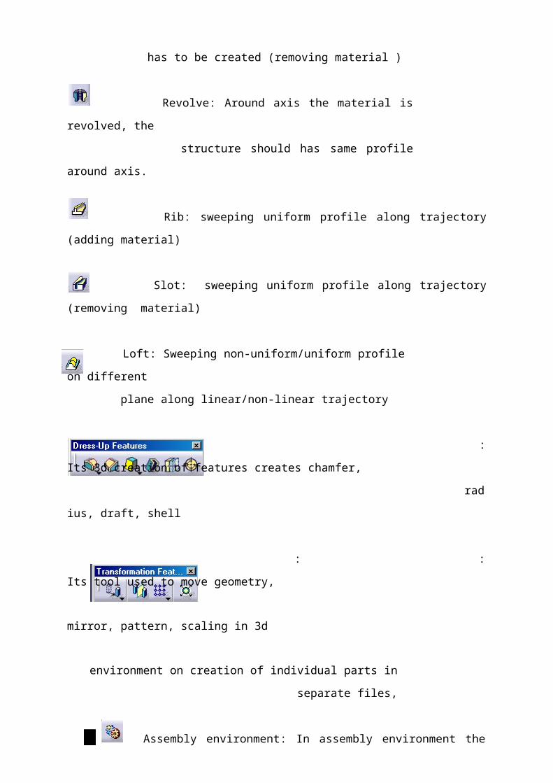
has to be created (removing material )
Revolve: Around axis the material is
revolved, the
structure should has same profile
around axis.
Rib: sweeping uniform profile along trajectory
(adding material)
Slot: sweeping uniform profile along trajectory
(removing material)
Loft: Sweeping non-uniform/uniform profile
on different
plane along linear/non-linear trajectory
:
Its 3d creation of features creates chamfer,
rad
ius, draft, shell
: :
Its tool used to move geometry, mirror, pattern, scaling in 3d
environment on creation of individual parts in
separate files,
Assembly environment: In assembly environment the

parts are recalled & constrained.
Product structure tool: To recall existing
components already modeled.
:Assembling respective parts by
mean of constraints
Update: updating the made constrains.
Additional features are: Exploded View, snap
shots, clash analyzing numbering, bill of
material. Etc
-22-
Finally creating draft for individual parts &
assembly with possible details
The parts of the major assembly is treated as individual
geometric model , which is modeled individually in separate
file .All the parts are previously planned & generated feature
by feature to construct full model
Generally all CAD models are generated in the same passion
given below:
: Enter CAD environment by clicking, later
into part designing
mode to construct model.

: Select plane as basic reference.
: Enter sketcher mode.
In sketcher mode:
: Tool used
to create 2-d basic structure of
part using
line, circle etc
: Tool used for editing of created
geometry termed as operation
: Tool used for Dimensioning,
referencing. This helps creating
parametric relation.
: Its external feature to view
geometry in & out
:Tool used to exit sketcher mode after creating geometry.
-23-

Sketch Based Feature:
Pad: On exit of sketcher mode the feature is to
be padded. (Adding material)
Pocket: On creation of basic structure further
pocket has to be created
(removing material)
Revolve: Around axis the material is revolved,
the structure
should have same profile around axis.
Rib: sweeping uniform profile along trajectory
(adding material)
Slot: sweeping uniform profile along trajectory
(removing material)
Loft: Sweeping non-uniform/uniform profile on
different plane along linear/non- linear
Trajectory
: Its 3d
creation of features creates chamfer,
radius
, draft shell, thread.
: This tool is used to move
geometry, mirror, pattern,
scali

ng in 3d environment.
-24-
5.0 Introduction of ANSYS:
This Tutorial will use a readymade file to speed up the
learning process for the student. This file is provided in
Parasolid format. The intention of this tutorial is to get the
student to run a straight forward simulation. By the end of
this tutorial a check list for the required procedure can be
formulated by the student. ANSYS as a software is made to be
user-friendly and simplified as much
as possible with lots of interface options to keep the
user as much as possible from the hectic side of
programming and debugging process.
Why is it that such a simple model is used?
During this tutorial a simple geometry is used, the objective

of that is that the student masters the steps to get to run a
simple simulation, once that’s done the student can model any
kind of geometry he sees necessary for his studied case.
Step1: Launch ANSYS ,by going to the start-up menu and double
clicking on workbench file in the ANSYS 13.0 folder.
Figure no:6 Step:1 in ANSYS
(A reminder that not all lab machines have the
ANSYS software installed on them.)
Step2: Once the program is launched it should look like as
shown below. Go to Analysis Systems;
Fluid Flow (CFX) and double click.

Figure7: Step:2 in ANSYS
(You might have to wait a bit till ANSYS gets running, the
student is encouraged to use the provided help with the
software, it has lots of useful hints here and there.)
Step3: Next Double click on the Geometry. This stage is for
getting the required geometry read into the software, note
that there is a blue question mark icon beside the geometry
text. Looking at the bottom of the window you will see two
windows one having the title of Messages, this title confirms
that the imported geometry has no problems with it, the next
window has the title Progress and
that is necessary to prove that state of the progress and if
there is a problem it will state the problem.

Figure8: Step:3 in ANSYS
(At the moment the illustration are a bit
simplified for the user and will get complex with
time.)
Step4: Once ANSYS Workbench window is active you will get a
window asking to specify working units for the model dimension
chose meters and press ok. For the user this step might seem
secondary in importance but as a matter of fact it’s of great
importance, because at later stages you will have to specify
the box size (discrete element dimension). Box size dimension
leads to finer mesh, the finer the used mesh is the more
accurate is the captured data. The captured data term refers
to the fluid flow structures.

Figure9: Step:4 in ANSYS
(Depending on your studied case the selection of
serial or parallel is taken, also depending on the
hardware provided in the computer lab dual core or
quad core etc.)

Step5: Go to file and choose Import External Geometry File…. .
Figure10: Step:5 in ANSYS
(You can model your geometry using the sketching tools
provided with Design Modeler.)

Step 6: A window having a title open will be visible to
the user, choose File type
Parasolid(*x_t;*xmt_txt;*x_b;*xmt_bin) then go to the
folder that has the required file .

Figure11: Step:6 in ANSYS
(There are lots of software that are used to generate meshes,
depending on the software used the file extension text would be,
in our case we are using SolidWorks to generate the mesh and then
exporting it in Parasolid format. A question comes to the mind of
the student why do I have to specify the file extension. The
answer is that each mesh generation software has its own structure
in its generated data sets. A simple example:)
Step7: Looking at the DesigModeler window, we can’t see the
imported geometry yet, what is required next is to press on
the generate icon that is represented by a yellow thunder
icon.

Figure12: Step:7 in ANSYS
(The DesignModeler will read in the imported data file, and
will construct the required mesh.Step7: The imported Geometry
Domain should look something like this, still that doesn’t
give any hints to the user, relating to the inner structure of
the domain.)

Step8: Go to the view and choose wire frame as shown below;
Figure13: Step:8 in ANSYS
(go to view and chose wireframe)

Step9: Go to the view and the inner structure of the domain as
shown below;
Figure14: Step:9 in ANSYS
(This step is necessary to view the inner structure of
the domain.)

Step9(a): Mouse options are shown below;
Figure15.1: Step:9(a) in ANSYS
(Once the student gets to this stage, that means he has
finished from the Design Modeler and has to proceed to the
Meshing part)

Figure15.2: Step:9(a) in ANSYS
(Rotate the view and check that the Geometry satisfies the
design requirements.)
Step 9(b): Go to the workbench and check that there is a green
tick sign beside the Geometry and then double click on the
Mesh Icon.

Figure15.3: Step:9(b) in ANSYS
(Congratulations you have finished from DesignModeler and now
have started with the Meshing part.)
Step 10: The Meshing part of the project has started,
notice that beside the Mesh there is a yellow thunder
icon.
Figure16: Step:10 in ANSYS

(The scale shown at the bottom helps you make the right
decision on the box sizing, sothat we can see that the
largest value on the scale is 0.200(m) which means we have to
choose a value less than 0.050(m).)
Step 10(a): right click on Mesh and chose Insert and then
chose Method

Figure16.1: Step:10(a) in ANSYS
(At this stage we come to the point where we have to choose
what kind of mesh are we going to use wither regular or
irregular or etc.)

Step 10(b): click on the positive sign beside the Mesh you
should get a tree sub branch have automatic Method using the
left button click on the grey box domain, as a result it
should by highlighted in green, then you see that the geometry
text is highlighted in blue press the apply.
Figure16.2: Step:10(b) in ANSYS
(Choose the parallel option in the projection mode, which
will come handy later on, when you want to use the
measure command or choosing the appropriate slice plane
for your study.)

Step 11: go to method and choose Tetrahedrons.
Figure17: Step:11 in ANSYS
(Now that you have specified the mesh properties, you can
proceed to the next step.)
Step12: press the Update icon and then press on the
Generate Mesh icon.

Figure18: Step:12 in ANSYS
(For our case we will want to now the dimensions of the
inflow section of the pipe.)
Step13: click on mesh, now it’s visible to the user the
generated mesh.
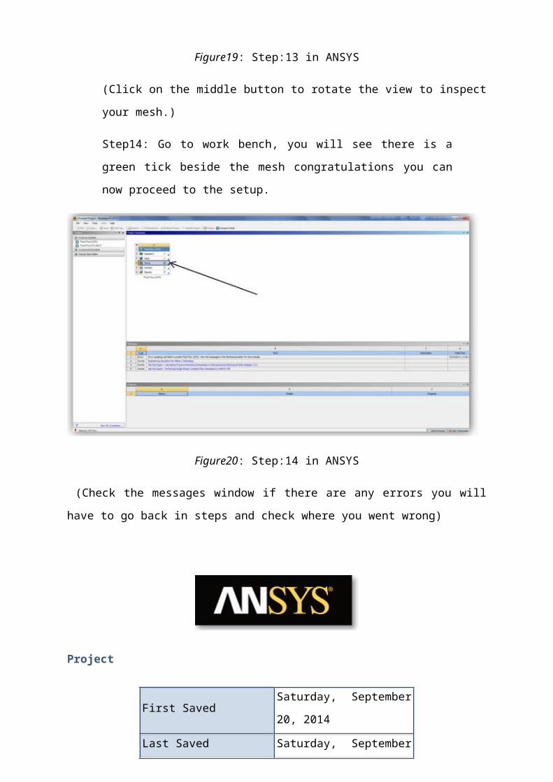
Figure19: Step:13 in ANSYS
(Click on the middle button to rotate the view to inspect
your mesh.)
Step14: Go to work bench, you will see there is a
green tick beside the mesh congratulations you can
now proceed to the setup.
Figure20: Step:14 in ANSYS
(Check the messages window if there are any errors you will
have to go back in steps and check where you went wrong)
Project
First SavedSaturday, September
20, 2014
Last Saved Saturday, September

20, 2014
Product Version 14.0 Release
Save Project Before
SolutionNo
Save Project After
SolutionNo

Contents
Units
Model (A4)
o Geometry
Parts
o Coordinate Systems
o Connections
o Mesh
o Static Structural (A5)
Analysis Settings
Loads
Solution (A6)
Solution Information
Results
Material Data
o Gray Cast Iron
o Structural Steel
Units
TABLE
1
Unit SystemMetric (mm, kg, N, s, mV, mA)
Degrees rad/s Celsius
Angle Degrees
Rotational
Velocityrad/s
Temperature Celsius
Model (A4)

Geometry
TABLE 2
Model (A4) > Geometry
Object Name Geometry
State Fully Defined
Definition
SourceC:\Users\sanju\Desktop\
worm ass.igs
Type Iges
Length Unit Meters
Element Control Program Controlled
Display Style Body Color
Bounding Box
Length X 183.39 mm
Length Y 215.7 mm
Length Z 48.001 mm
Properties
Volume 74736 mm³
Mass 0.5381 kg
Scale Factor Value 1.
Statistics
Bodies 2
Active Bodies 1
Nodes 5767
Elements 3088
Mesh Metric None
Basic Geometry Options
Solid Bodies Yes
Surface Bodies Yes

Line Bodies No
Parameters Yes
Parameter Key DS
Attributes No
Named Selections No
Material Properties Yes
Advanced Geometry Options
Use Associativity Yes
Coordinate Systems No
Reader Mode Saves
Updated FileNo
Use Instances Yes
Smart CAD Update No
Attach File Via Temp
FileYes
Temporary DirectoryC:\Users\sanju\AppData\
Local\Temp
Analysis Type 3-D
Mixed Import Resolution None
Decompose Disjoint Faces Yes
Enclosure and Symmetry
ProcessingYes
TABLE 3
Model (A4) > Geometry > Parts
Object Name Part 1 Part 2
State Meshed Suppressed
Graphics Properties
Visible Yes No
Transparency 1

Definition
Suppressed No Yes
Stiffness
BehaviorFlexible
Coordinate
System
Default Coordinate
System
Reference
TemperatureBy Environment
Material
AssignmentGray Cast
Iron
Structural
Steel
Nonlinear
EffectsYes
Thermal Strain
EffectsYes
Bounding Box
Length X 60. mm 183.39 mm
Length Y 48.002 mm 183.39 mm
Length Z 48.001 mm 20.001 mm
Properties
Volume 74736 mm³3.9619e+005
mm³
Mass 0.5381 kg 3.1101 kg
Centroid X1.842e-002
mm
7.5693e-007
mm
Centroid Y 100.3 mm1.6878e-006
mm
Centroid Z2.4372e-003
mm
2.2837e-005
mm
Moment of 118.31 5058.8

Inertia Ip1 kg·mm² kg·mm²
Moment of
Inertia Ip2
213.23
kg·mm²
5058.8
kg·mm²
Moment of
Inertia Ip3
213.71
kg·mm²
9910.3
kg·mm²
Statistics
Nodes 5767 0
Elements 3088 0
Mesh Metric None
Coordinate Systems
TABLE 4
Model (A4) > Coordinate Systems > Coordinate System
Object NameGlobal Coordinate
System
State Fully Defined
Definition
Type Cartesian
Coordinate
System ID0.
Origin
Origin X 0. mm
Origin Y 0. mm
Origin Z 0. mm
Directional Vectors
X Axis Data [ 1. 0. 0. ]
Y Axis Data [ 0. 1. 0. ]
Z Axis Data [ 0. 0. 1. ]
Connections

TABLE 5
Model (A4) > Connections
Object Name Connections
StateFully
Defined
Auto Detection
Generate Automatic Connection
On RefreshYes
Transparency
Enabled Yes
Mesh
TABLE 6
Model (A4) > Mesh
Object Name Mesh
State Solved
Defaults
Physics Preference Mechanical
Relevance 0
Sizing
Use Advanced Size
FunctionOff
Relevance Center Medium
Element Size Default
Initial Size Seed Active Assembly
Smoothing Medium
Transition Fast
Span Angle Center Coarse
Minimum Edge Length 0.256690 mm
Inflation

Use Automatic Inflation None
Inflation OptionSmooth
Transition
Transition Ratio 0.272
Maximum Layers 5
Growth Rate 1.2
Inflation Algorithm Pre
View Advanced Options No
Patch Conforming Options
Triangle Surface MesherProgram
Controlled
Advanced
Shape CheckingStandard
Mechanical
Element Midside NodesProgram
Controlled
Straight Sided Elements No
Number of Retries Default (4)
Extra Retries For
AssemblyYes
Rigid Body BehaviorDimensionally
Reduced
Mesh Morphing Disabled
Defeaturing
Pinch Tolerance Please Define
Generate Pinch on
RefreshNo
Automatic Mesh Based
DefeaturingOn

Defeaturing Tolerance Default
Statistics
Nodes 5767
Elements 3088
Mesh Metric None
Static Structural (A5)
TABLE 7
Model (A4) > Analysis
Object NameStatic Structural
(A5)
State Solved
Definition
Physics Type Structural
Analysis TypeStatic
Structural
Solver TargetMechanical
APDL
Options
Environment
Temperature22. °C
Generate Input
OnlyNo
TABLE 8
Model (A4) > Static Structural (A5) > Analysis Settings

Object Name Analysis Settings
State Fully Defined
Step Controls
Number Of
Steps1.
Current Step
Number1.
Step End Time 1. s
Auto Time
SteppingProgram Controlled
Solver Controls
Solver Type Program Controlled
Weak Springs Program Controlled
Large
DeflectionOff
Inertia
ReliefOff
Restart Controls
Generate
Restart
Points
Program Controlled
Retain Files
After Full
Solve
No
Nonlinear Controls
Force
ConvergenceProgram Controlled
Moment
ConvergenceProgram Controlled
Displacement Program Controlled

Convergence
Rotation
ConvergenceProgram Controlled
Line Search Program Controlled
Stabilization Off
Output Controls
Stress Yes
Strain Yes
Nodal Forces No
Contact
MiscellaneousNo
General
MiscellaneousNo
Calculate
Results AtAll Time Points
Max Number of
Result SetsProgram Controlled
Analysis Data Management
Solver Files
Directory
C:\Users\sanju\AppData\Local\Temp\WB_SANJU-
PC_5892_2\unsaved_project_files\dp0\SYS\MECH\
Future
AnalysisNone
Scratch
Solver Files
Directory
Save MAPDL db No
Delete
Unneeded
Files
Yes
Nonlinear No
Solution
Solver Units Active System
Solver Unit
Systemnmm
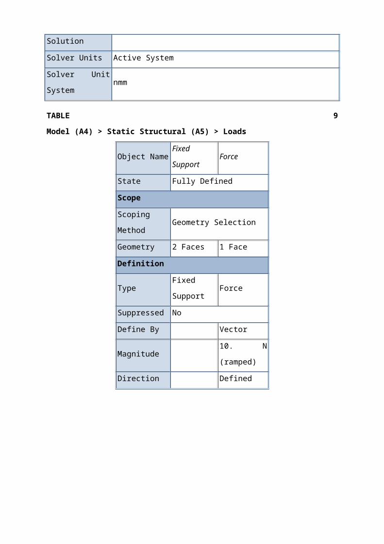
TABLE 9
Model (A4) > Static Structural (A5) > Loads
Object NameFixed
SupportForce
State Fully Defined
Scope
Scoping
MethodGeometry Selection
Geometry 2 Faces 1 Face
Definition
TypeFixed
SupportForce
Suppressed No
Define By Vector
Magnitude 10. N
(ramped)
Direction Defined

FIGURE 1
Model (A4) > Static Structural (A5) > Force
Solution (A6)
TABLE 10
Model (A4) > Static Structural (A5) > Solution
Object NameSolution
(A6)
State Solved
Adaptive Mesh Refinement
Max Refinement
Loops1.
Refinement 2.
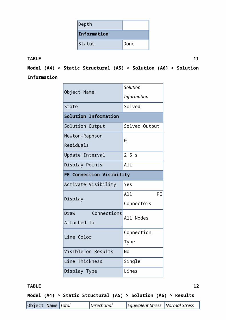
Depth
Information
Status Done
TABLE 11
Model (A4) > Static Structural (A5) > Solution (A6) > Solution
Information
Object NameSolution
Information
State Solved
Solution Information
Solution Output Solver Output
Newton-Raphson
Residuals0
Update Interval 2.5 s
Display Points All
FE Connection Visibility
Activate Visibility Yes
DisplayAll FE
Connectors
Draw Connections
Attached ToAll Nodes
Line ColorConnection
Type
Visible on Results No
Line Thickness Single
Display Type Lines
TABLE 12
Model (A4) > Static Structural (A5) > Solution (A6) > Results
Object Name Total Directional Equivalent Stress Normal Stress
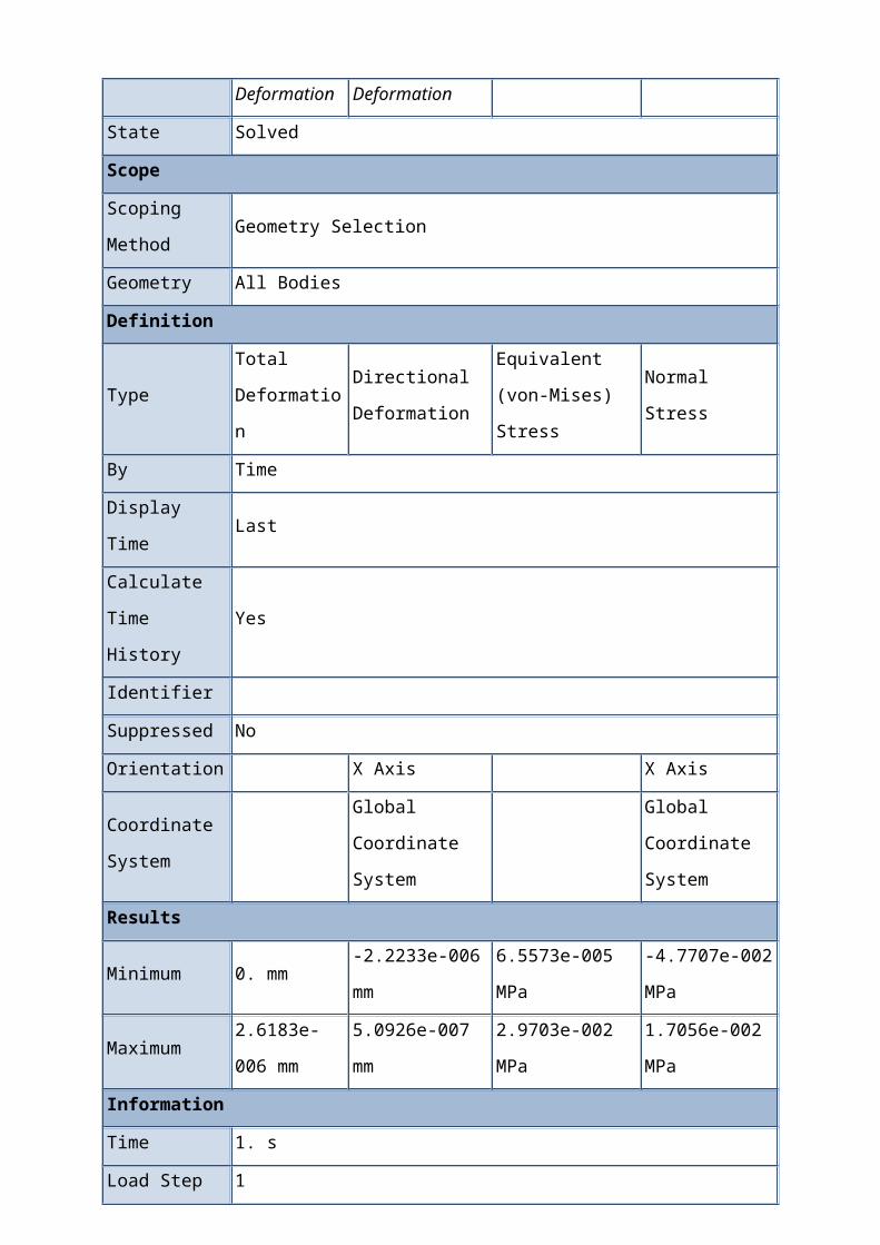
Deformation Deformation
State Solved
Scope
Scoping
MethodGeometry Selection
Geometry All Bodies
Definition
Type
Total
Deformatio
n
Directional
Deformation
Equivalent
(von-Mises)
Stress
Normal
Stress
By Time
Display
TimeLast
Calculate
Time
History
Yes
Identifier
Suppressed No
Orientation X Axis X Axis
Coordinate
System
Global
Coordinate
System
Global
Coordinate
System
Results
Minimum 0. mm-2.2233e-006
mm
6.5573e-005
MPa
-4.7707e-002
MPa
Maximum2.6183e-
006 mm
5.0926e-007
mm
2.9703e-002
MPa
1.7056e-002
MPa
Information
Time 1. s
Load Step 1

Substep 1
Iteration
Number1
Integration Point Results
Display
Option Averaged
FIGURE 2
Model (A4) > Static Structural (A5) > Solution (A6) > Total
Deformation > Figure


FIGURE 3
Model (A4) > Static Structural (A5) > Solution (A6) >
Directional Deformation > Figure

FIGURE 4
Model (A4) > Static Structural (A5) > Solution (A6) >
Equivalent Stress > Figure
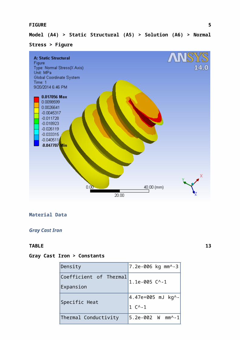
FIGURE 5
Model (A4) > Static Structural (A5) > Solution (A6) > Normal
Stress > Figure
Material Data
Gray Cast Iron
TABLE 13
Gray Cast Iron > Constants
Density 7.2e-006 kg mm^-3
Coefficient of Thermal
Expansion1.1e-005 C^-1
Specific Heat4.47e+005 mJ kg^-
1 C^-1
Thermal Conductivity 5.2e-002 W mm^-1

C^-1
Resistivity 9.6e-005 ohm mm
TABLE 14
Gray Cast Iron > Compressive Ultimate Strength
Compressive Ultimate
Strength MPa
820
TABLE 15
Gray Cast Iron > Compressive Yield Strength
Compressive Yield
Strength MPa
0
TABLE 16
Gray Cast Iron > Tensile Yield Strength
Tensile Yield
Strength MPa
0
TABLE 17
Gray Cast Iron > Tensile Ultimate Strength
Tensile Ultimate
Strength MPa
240
TABLE 18
Gray Cast Iron > Isotropic Secant Coefficient of Thermal
Expansion
Reference
Temperature C

22
TABLE 19
Gray Cast Iron > Isotropic Elasticity
Temperatu
re C
Young's
Modulus MPa
Poisson's
Ratio
Bulk Modulus
MPa
Shear Modulus
MPa
1.1e+005 0.28 83333 42969
TABLE 20
Gray Cast Iron > Isotropic Relative Permeability
Relative
Permeability
10000
Structural Steel
TABLE 21
Structural Steel > Constants
Density7.85e-006 kg mm^-
3
Coefficient of Thermal
Expansion1.2e-005 C^-1
Specific Heat4.34e+005 mJ kg^-
1 C^-1
Thermal Conductivity6.05e-002 W mm^-1
C^-1
Resistivity 1.7e-004 ohm mm

TABLE 22
Structural Steel > Compressive Ultimate Strength
Compressive Ultimate
Strength MPa
0
TABLE 23
Structural Steel > Compressive Yield Strength
Compressive Yield
Strength MPa
250
TABLE 24
Structural Steel > Tensile Yield Strength
Tensile Yield
Strength MPa
250
TABLE 25
Structural Steel > Tensile Ultimate Strength
Tensile Ultimate
Strength MPa
460
TABLE 26
Structural Steel > Isotropic Secant Coefficient of Thermal
Expansion
Reference
Temperature C
22

TABLE 27
Structural Steel > Alternating Stress Mean Stress
Alternating
Stress MPa
Cycle
s
Mean Stress
MPa
3999 10 0
2827 20 0
1896 50 0
1413 100 0
1069 200 0
441 2000 0
262 10000 0
214 20000 0
1381.e+0
050
1142.e+0
050
86.21.e+0
060
TABLE 28
Structural Steel > Strain-Life Parameters
Strength
Coefficien
t MPa
Strength
Exponent
Ductility
Coefficie
nt
Ductilit
y
Exponent
Cyclic
Strength
Coefficient
MPa
Cyclic
Strain
Hardening
Exponent
920 -0.106 0.213 -0.47 1000 0.2
TABLE 29
Structural Steel > Isotropic Elasticity
Temperatu
re C
Young's
Modulus MPa
Poisson's
Ratio
Bulk Modulus
MPa
Shear
Modulus MPa

2.e+005 0.3 1.6667e+005 76923
TABLE 30
Structural Steel > Isotropic Relative Permeability
Relative
Permeability
10000