INTERNATIONAL CONFERENCE ON WHEEL/RAIL LOAD ...

PROCEEDINGSINTERNATIONAL CONFERENCE ON

WHEEL/RAIL LOAD AND DISPLACEMENT MEASUREMENT TECHNIQUES

January 19-20, 1981

Edited By

Pin Tong and R obert G reif

S ep tem ber 1981

Sponsored By

oU.S. Department of Transportation I *

TRANSPO RT C A N A D A

NOTICE

This document is disseminated under the sponsorship of the Department of Transportation in the interest of information exchange. The United States Government assumes no liability for its contents or use thereof.

NOTICE

The United States Government does not endorse products or manufacturers. Trade or manufacturers' names appear herein solely because they are considered essential to the object of this report.

US. Departm ent of Transportation

Transportation Systems Center

Kendall SquareCambridge, Massachusetts 02142

Research and Special Programs Administration

February 5, 1982

Dear Colleague,

Enclosed are the Proceedings of the "International Conference

on Wheel/Rail Load and Displacement Measurement Techniques" which

was held at the Transportation Systems Center in January 1981.

The objective of the Conference was to review the state-of-the-art

and provide a forum for information exchange in the field of

wheel/rail loading and movement of track due to vehicle and track

interaction under diverse loading conditions. Your participation

in the Conference helped us to attain this goal and led to a

valuable interchange of technical information. I trust you will

find these Proceedings useful in your work.

I also hope we can continue these forums for technical

interchange. I am proposing another symposium on some areas in

railroad technology to be held in the near future, perhaps in

late '83. I would welcome any suggestions as to the sponsors

and organizers for this next meeting.

Sincerely

Pin Tong, ChiefStructures \.and Mechanics Branch

Enclosure

DOT-TSC-UMTA-82-3

PROCEEDINGSINTERNATIONAL CONFERENCE ON

WHEEL/RAIL LOAD AND DISPLACEMENT MEASUREMENT TECHNIQUES

January 19-20, 1981

Edited By

Pin Tong and R obert G re if

Sponsored By

U.S. DEPARTM ENT OF TRANSPO R TATIO NFederal Railroad A d m in is tra tio n

O ffice o f Research and D eve lopm en t

Research and Special P rogram s A d m in is tra tio n O ffice o f U n ive rs ity Research

Urban M ass T ranspo rta tion A d m in is tra tio n O ffice o f Rail and C o ns truc tion T echno log y

TRANSPO RT C A N A D A T ranspo rta tion D eve lopm en t C entre

S ep tem be r 1981

U.S. DEPARTMENT OF TRANSPORTATION Research and Specia l P rogram s A d m in is tra tio n

T ranspo rta tion System s C enter Kendall Square

C am bridge , M assachuse tts

INTERNATIONAL CONFERENCE ON WHEEL/RAIL LOAD AND DISPLACEMENT MEASUREMENT TECHNIQUES

TABLE OF CONTENTS

PAGEINTRODUCTION......................................... 1P. Tong, R. Greif

WELCOME.............................................. 7Robert J. Ravera

PAPER NO. SESSION 1: WHEEL/RAIL LOAD MEASUREMENT TECHNIQUES - IChairman: N.T. Tsai

1. MEASUREMENT TECHNIQUES FOR ONBOARD WHEEL/RAIL LOADS... 1-1J.K. Kesler, Ta-Lun Yang, and P. Boyd

2. DEVELOPMENT OF A WHEEL/RAIL MEASUREMENT SYSTEM - FROMCONCEPT TO UTILIZATION............ 2-1G. B. Bakken, D.W. Gibson and R.A. Peacock

3. DEVELOPMENT AND USE OF AN INSTRUMENTED WHEELSET FORTHE MEASUREMENT OF WHEEL/RAIL INTERACTION FORCES..... 3-1M.R. Johnson

4. THE B.R. LOAD MEASURING WHEEL........................ 4-1A.R. Pocklington

5. DEVELOPMENT AND USE OF INSTRUMENTED LOCOMOTIVE WHEEL-SETS................................................. 5-1C.A. Swenson and K.R. Smith

6. CALIBRATION GUIDELINES AND EQUIPMENT, IMPORTANT CHARACTERISTICS AND ERROR TYPES FOR INSTRUMENTEDWHEELSETS........................................... 6-1T.J. Anderson

7. DETERMINATION'OF WHEEL/RAIL FORCES BY MEANS OF MEASURINGWHEELSETS ON THE DEUTSCHE BUNDESBAHN (DB)........... 7-1H-H. Zuck

SESSION 2: WHEEL/RAIL LOAD MEASUREMENT TECHNIQUES - IIChairman: P.R. Spencer

8. DEVELOPMENT AND EVALUATION OF WAYSIDE WHEEL/RAIL LOADMEASUREMENT TECHNIQUES.............................. 8-1H. D. Harrison and D.R. Ahlbeck

i

WAYSIDE MONITORING OF WHEEL/RAIL LOADS S.R. Benton

PAGE9.

10.

11.

12.

9-1

RAIL LOAD MEASUREMENTS ON SUBWAY SYSTEMS............ 10-1J.R. Billing

SPECTRAL ANALYSIS OF FREIGHT CAR TRUCK LATERALRESPONSE IN DYNAMICALLY SCALED MODEL EXPERIMENTS.... 11-1L.M. Sweet and A. Karmel

FREIGHT EQUIPMENT ENVIRONMENT SAMPLING TEST - CENTERPLATE AND SIDE BEARING LOADS FOR FATIGUE ANALYSIS___ 12-1S. Richmond, W.H. SneedFilm: "The Construction of the Chengtu-Kunming Railway"

Reception and Dinner MIT Faculty ClubSpeaker: L.M. Sweet, Princeton University"Overview of Railroad Technology and Research in Japan"

SESSION 3: DISPLACEMENT AND GEOMETRY MEASUREMENT TECHNIQUESChairman: D.W. Dibble

13. THE USE OF ANGLE-OF-ATTACK MEASUREMENTS TO ESTIMATE RAILWEAR UNDER STEADY-STATE ROLLING CONDITIONS.......... 13-1H. Ghonem, J. Kalousek

14. MEASUREMENT, PROCESSING,MD USE OF WHEEL-RAIL GEOMETRICCONSTRAINT FUNCTIONS...................... ......... 14-1E.H. Law, N.K. Cooperider, J.M. Tuten

15. MECHANICAL SYSTEMS MEASURING TECHNIQUES FOR TRACKGEOMETRY............................................ 15-1G. Oberlechner

16. INERTIAL AND'INDUCTIVE MEASUREMENT TECHNIQUES FORTRACK GEOMETRY....... ...... ........................ 16-1Ta-Lun Yang, E.D. Howerter, and R.L. Inman

17. MEASUREMENT OF TRACK PROFILE IRREGULARITIES......... 17-1L . Lin

18. USE OF THE FINDINGS FROM RAIL-WEAR MEASUREMENTS FORRAILROAD TRACK DIAGNOSTICS......................... 18-1H. Baluch

19. REQUIREMENTS AND TECHNIQUES FOR MEASURING DYNAMICDISPLACEMENTS OF RAILROAD TRACK COMPONENTS.......... 19-1D.R. Ahlbeck, F.E. Dean

ii

PAGESESSION 4; PROBLEMS, OPPORTUNITIES, FUTURE NEEDS,AND TRENDS Chairman: S.C. ChuPanel Discussion................................... 20-1Film: "The Construction of the Chengtu-Kunming Railway"

CONFERENCE PARTICIPANTS............................ 21-1

i i i / i v

INTRODUCTION

Pin Tong

R. Greif


The International Conference on Wheel/Rail Load and Displacement

Measurement Techniques was held at the Transportation Systems Center (TSC) on

January 19-20, 1981. The Conference was sponsored by the U.S. Department of

Transportation (DOT) and Transport Canada. The U.S. DOT agencies involved in

the sponsorship include the Urban Mass Transportation Administration (UMTA),

the Federal Railroad Administration (FRA), and the Research and Special

Programs Administration (RSPA). The objective of the Conference was to review

the state-of-the-art and provide a forum for information exchange in the field

of wheel/rail loading and movement of track due to vehicle/track interactions

under diverse loading conditions.

The Conference was attended by over 125 railroad and transit industry,

Government and research experts from around the world. The Conference con

sisted of four sessions and 19 technical papers were presented by invited

speakers. Session 1 was devoted exclusively to instrumented wheelsets for

load measurement. Session 2 included technical papers on wayside measurements,

Session 3 examined track displacement and geometry measurement techniques,

while Session 4 was a Panel Discussion examining problems and future needs.

The format of the Panel enabled experts from various countries including the

1

United States, Canada, England, West Germany, Poland, Sweden, Austria and the

People's Republic of China to discuss the common theme of wheel/rail load and

displacement measurement in a more informal setting.

The technical sessions of the Conference were chaired by N.T. Tsai (FRA),

P. Spencer (UMTA), D.W. Dibble (Transport Canada) and S.C. Chu (RSPA). The

organizing committee which helped ensure the success of the meeting included

W.I. Thompson (TSC) and L. Foster (Raytheon Service Co.).

These bound Proceedings include a complete record of the panel discussion,

the technical papers and the accompanying question and answer discussion

period after each paper. The Conference also incuded an hour long film from

the People's Republic of China on "The Construction of the Chengtu-Kunming

Railway," as well as a reception and dinner at the MIT Faculty Club. The

featured speaker at the dinner was Prof. L.M. Sweet of Princeton University

who discussed the "Overview of Railroad Technology and Research in Japan."

As discussed by Dr. Ravera in his welcoming remarks, the Transportation

Systems Center is involved in research and development activities in all

fields of transportation. Since its inception in 1970, TSC has been exten

sively involved with problems related to wheel/rail interaction and has

cooperated with the co-sponsors of this. Conference — UMTA, FRA and RSPA — on

many engineering problems. The measurement of wheel/rail characteristics

generates information for improvement of design tools such as model valida

tion, establishment of load spectra and vehicle/track system interaction.

Existing and new designs are assessed from evaluation of vehicle/track degra

dation and performance measures associated with dynamic behavior, fuel economy

2

and safety parameters. The diagnosis and verification of hypotheses dealing

with track and carbody hunting, rock and roll, wheel climb, wear, and rail

strength has been instrumental in the introduction of new types of trucks,

such as radial or self-steering trucks, into prototype and day-to-day design

and operation.

Personnel of the Transportation Systems Center have been involved in many

Government/industry cooperative research and development efforts for the meas

urement of wheel/rail interactions including on-board measurements and wayside

measurements. These include test programs performed at the Transportation

Test Center (TTC) in Pueblo, Colorado, and at various field test sites on

operating railroads and transit properties. Among these test programs were

the Perturbed Track Tests (PTT) which investigated the dynamic response of

vehicles due to track perturbations, the Tests on Chessie System Track which

compared the performance of SDP-40F and E-8 locomotives, and the Vehicle/Track

Interaction Tests at Starr, Ohio, which investigated limiting conditions for

low speed operation of vehicles. Tests on transit properties include the

Washington Metropolitan Area Transit Authority (WMATA) for the assessment of

wheel/rail load and wear characteristics. Tests on the Port Authority Transit

Corporation (PATCO) were done to assess the effect of steerable trucks on

curving performance, lateral stability and ride quality.

Some of these test programs have led to improvements in instrumentation

design. For example, in the Chessie System Tests mentioned previously, it was

found that the ORE wayside gage circuit that was in common use at the time

recorded lateral forces that were substantially different than the lateral

forces predicted from the on-board measurement of the instrumented wheelset.

3

Upon an investigation by TSC, it was discovered that the formulation of the

circuit, which assumed that the cross-section of the rail behaved like a long

cantilever beam, was in error. The non-beamlike behavior leads to a substan

tial "cross-talk" arising from the response of the circuit to vertical load.

A combined TSC/Battelle team was formed to measure the strains throughout the

circumference of a rail cross-section under lateral and vertical loads in the

laboratory. Based on a review of laboratory data of strain distribution for

the loaded rail, Chessie System Test data, and additional data generated under

TSC's rail stress analysis projects, a number of alternative circuits were

identified for accurately measuring lateral rail loading. Against the cri

teria of sensitivity to.load, insensitivity to support conditions, linearity

and cross-talk, a base chevron circuit was selected as the best overall trans

ducer array. The newly developed base chevron circuit has a number of advan

tages over the old ORE web circuit for measuring lateral loads, the most sig

nificant being the order of magnitude reductions in cross-talk which it

permits. The additional advantages of this new circuit include:

(a) The gages are mounted on the top surface of the rail base, which allows easy installation in the field.

(b) Both lateral gage chevrons may be mounted over the same crib as the measurement circuit for vertical loads. This will enable the simultaneous measurement of the vertical and lateral loads with no phase shift.

This is just one example of the involvement of TSC in the development of

measurement techniques for wheel/rail interaction phenomena and in the broad

application of these measured values. Through its research and development

activities, TSC is looking forward to a continuing contribution to the safe

and economic operation of railroad and transit systems.

4

Advancements in the field of wheel/rail load and displacement measurement

techniques have been contributed by organizations from all over the world.

This Conference has provided a look at international developments in the cur

rent state-of-the-art in this field. From the papers presented at this

Conference, it is evident that instrumented wheelsets for load measurements

have reached an advanced stage of sophistication. There are several versions

of design in use today. The accuracy and frequency response of the commonly

used wheelsets are adequate for most vehicle/track systems dynamics studies,

and also for the assessment and diagnosis of the performance of existing or

new equipment. However, an instrumented wheelset is generally delicate and

complicated, requiring sophisticated electronics and associated data recording

systems, as well as highly trained personnel for its operation. Consequently,

future developments of instrumented wheelsets should emphasize simplification

of instrumentation and reduction of costs for operation of the system. In the

area of wayside load measurement, the TSC/Battelle lateral circuit and the ORE

vertical circuit have received wide acceptance. Direct comparison of on-board

and wayside measured loads has provided added confidence in the accuracy of

both measurements. The direct wayside measurements of rail motion seem to be

well under control. However, there has been little development of the measure

ment of wheel motion relative to a rail. These are important parameters for

the assessment of wheel/rail wear and wheel climb leading to derailment.

We expect great and rapid advancements in the measurement of wheel/rail

interaction. As we progress into the future with advanced instrumentation and

electronics, criteria for assessment need to be developed. Considerations in

the criteria should include cost, accuracy, simplicity of use and maintenance.

5

simplicity in trouble-shooting and finding errors, and longevity of the trans

ducer. Hopefully, this Conference with its attendant discussion and inter

change of information among various international groups will hasten develop

ments in this direction.

6

WELCOMERobert J. Ravera, Deputy Director


Good morning, ladies and gentlemen. On behalf of Dr. Costantino and the entire TSC staff, I'd like to welcome you to the Transportation Systems Center and to this International Conference on Wheel/Rail Load and Displacement Measurement Techniques.

I would particularly like to welcome our foreign visitors, some of whom have traveled such great distances. I understand that we have participants from research organizations and from the railroad and transit industries in England, Germany, Poland, Sweden and China, as well as from the United States and Canada.

This two day meeting is co-sponsored by the U.S. Department of Transportation and Transport Canada. In DOT, there are three agencies involved in the sponsorship of this conference: the Office of Research and Developmentof the Federal Railroad Administration, the Office of University Research of the Research and Special Programs Administration, and the Office of Rail and Construction Technology of the Urban Mass Transportation Administration.The Transportation Development Center is the sponsoring agency within Transport Canada.

It might be helpful at the beginning of this workship to give you a very brief overview of our role here in Cambridge, especially as it pertains to rail research and development. The Transportation Systems Center is DOT's research, analysis, and development facility for its major programs in air, rail, motor vehicle, pipeline, and marine transportation. With an annual budget of some 70 million dollars and a staff of approximately 1 thousand federal employees and onsite support serivce contractors, we carry out major research, analysis and development programs for the Office of the Secretary of Transportation and for all the administrations within DOT. To a lesser degree, we also perform research for other government agencies, such as the Department of Energy, Environmental Protection Agency, etc., when such research complements ongoing work for the Department of Transportation. We also provide state and local governments and private industry with engineering, economic and planning information for all types of transportation programs through our Technology Sharing Office. We currently have about 200 research projects underway.

Since its opening in 1970, TSC has supported programs of all elements of the Federal Rail Administration. This support has been funded at over 60 million dollars during these ten years. It has ranged in scope from participation in the solution of short-term technical problems to the longterm technical management of major rail R and D programs. TSC railroad related projects cover both the engineering aspects of railroad operation as well the economic and institutional analyses supporting federal policy initiatives.

7

Projects span the spectrum from improved track safety standards and track inspection vehicles to safety improvements, options analyses, and the impact of all federal transportation policies on the railroads. We are presently engaged in several programs related to the subject of wheel/rail loads such as a stability assessment facility for equipment (the SAFE faci-r lities) for Federal Railroad Administration.

Much of the R and D support we provide for the Urban Mass Transportation Administration is also related to problems associated with wheel/rail interaction. This includes urban rail noise studies, derailments of the light rail vehicles in Boston, and studies of wheel/rail wear, particularly problems arising from recent truck designs. Speaking of truck designs, projects involving radial or self-steering trucks have been underway for sometime for both UMTA and FRA. These development programs have also prompted the requirement for a better understanding of wheel/rail load and displacement measurement techniques. In the next two days, we will have an opportunity to exchange information on this subject.

TSC over the years has also supported, in a very major way, studies and analyses on all forms of urban transportation projects for UMTA, including bus technology, bus demonstration programs, fare collection, and service and methods. Our relationship with UMTA has been a very long and, I think, a mutually profitable one.

At this point, I think it is appropriate for me to conclude my remarks and wish you a stimulating, enjoyable and successful conference. Thank you.

8

SESSION 1: WHEEL/RAIL LOAD MEASUREMENT TECHNIQUES - I

MEASUREMENT TECHNIQUES FOR ONBOARD WHEEL/RAIL LOADS

Patrick Boyd Kevin Kesler Ta-Lun Yang

ENSCO, INC.5408A Port Royal Rd.

Springfield, VA 22151

1. Introduction

For the determination of rail vehicle wheel forces both direct force measure

ment and inertial force measurement techniques should be considered. Direct

force measurement techniques include instrumented wheelsets and journal

load cells. Inertial force measurement is performed by measuring the accel

erations of the major vehicle components (i.e., wheelsets, trucks and car-

body) and multiplying by the effective mass of each. Depending upon the

goals of a particular test program any of the approaches may be best applied.

For example, if steady response is of interest only direct force measurement

can be applied. Creep force measurement and dynamic wheel forces require

instrumented wheelsets. Dynamic truck and axle forces can be measured with

instrumented wheelsets or a combination of journal load cells and accelerome

ters. Table 1.1, "Applications of Force Measurement Techniques", summarizes

which techniques may be applied to each measurement task. In many cases

instrumented wheelsets can be supplemented or replaced by another technique

for a more thorough or cost effective measurement.

Even though instrumented wheelsets provide the most accurate measurement of

wheel/rail forces they are somewhat limited in analyzing vehicle response.

Inertial force measurement can be used to provide valuable insight into the

modes and mechanisms which generated the measured wheel/rail forces.

1 - 1

2. Journal Load Cell

2.1 Design Considerations

Many railroad trucks, especially locomotive trucks, are designed to transmit

lateral forces between the truck frame and the axles through thrust bearings

installed at the ends of the axles. With this type of design, the load path

for a lateral force goes from a wheel flange through the axle to the thrust

bearing on the opposite end of the axle and continues through the bearing

housing and to the truck frame. For instance, the steady-state curving force

in a left-hand curve is applied to the flange on the right wheel, the force

is transmitted through the wheel plate, the axle and to the thrust bearing at

the left end of the axle. The force is then transmitted from the thrust

bearing through the bearing cap, the bearing housing and to the truck frame

which in turn passes the force thrugh the bolster, centerplate and eventually

to the carbody.

Since the thrust bearing is a focalized point in the lateral load path,

specially designed load cells have been used to fit in the space normally

occupied by the thrust bearings for measuring the lateral force transmitted

through that point. In testing of locomotive dynamics, EMD has used this

technique on many types of trucks employing non-rotating bearing end-caps.

The advantages of this measuring technique are that the measurement is made

in the iine of the load path, it introduces a minimal modification to the

mechanical characteristics of the truck, the end-cap/thrust bearing load cell

can be pre-assembled and installed in any vehicle quickly and the output is a

direct continuous measurement of the lateral force which requires no special

processing.

This measurement approach is limited to the type of trucks which use the

thrust bearing design or can be modified to accept such a bearing. Further

more, there are certain disadvantages. Since the thrust bearing and the

wheel-rail contact points are separated by the wheel and axle set, the in

ertial forces due to lateral movements of the wheel and axle mass, including

the traction motor and gear box, are not measured by the thrust bearing load

1-2

cell even though they contribute to the lateral forces at the wheel-rail

contact points. Because of the built-in freeplay betwen the wheelset and the

truck frame, at most one of the two thrust bearings will be carrying a lateral

load at any time. The force as measured by the load cell in action is repre

sentative of the total lateral force applied to the axle from the truck frame

and should be equal and opposite to the sum of the lateral forces applied

through the wheel-rail contact points on both wheels (except for the inerial

forces due to lateral accelerations of the axle mass as discussed above). It

is therefore not possible to resolve the lateral force at each wheel-rail

contact point. In Figure 2-1, the lateral forces acting on a single axle are

shown for an instant when the axle is experiencing a lateral acceleration x.

Assuming that the wheel axle set and the components that are fastened to the

axle are moving together at the same acceleration, then the inertial force

can be represented by Mx, with M being the total mass in the wheel-axle

assembly. The dynamic force equilibrium in the lateral direction implies

that:

= FRF + Frc + F^c + Mx + MgSinG

in which Hl is the force measured by the thrust bearing load cell on the left

end of the axle, Fjyp is the flange contact force on the right wheel, Frq and

Flc are the creep forces on the right and left wheel tread, Mx is the inertial

force due to lateral dynamics and MgSinG is the gravitational force component

due to track crosslevel G. It should be noted that the inertial acceleration

x may contain a component caused by steady-state curving and a component by

pure lateral translation. The steady-state translational component will be

oscillatory in nature and of a relatively high frequency.

The equation given above and Figure 2-1 can also be used to illustrate the

difference betwen the load cell technqiue and the instrumented wheel tech

niques. Instrumented wheels, with the strain gages located in the wheel-

plates or spokes, will measure the forces (Fpp + Fr q ) an^ FLC directly. the

only portion of the force not measured by instrumented wheels are the con

tributions to the inertial forces from the mass in the wheel rims.

1-3

3. Inertial Measurement Technique

A major contributor to the lateral wheel-rail force is the dynamic motions

of a vehicle perpendicular to the direction of travel. These motions pro

duce forces which are directly relatable to the mass components and their

inertial accelerations in the lateral direction. Researchers have installed

accelerometers on vehicle mass components in an attempt to estimate the

wheel-rail forces from acceleration measurements. These attempts were

often unsuccessful due to several difficulties: the choice of a suitable9

transducer and the proper mounting bracket due to the high frequency and

high levels of shock and vibrations in the truck, the assignment of an

"effective mass" to each measured acceleration due to the presence of

simultaneous linear and rotational motions, and the lack of a reliable

independent force measuring technique to verify the results.

In order to successfully collect the acceleration data on each mass element

in the vehicle and truck which contributes to lateral inertial force, an

appropriate transducer must be used on each of the mass components to ac

commodate the different vibration environments and the different character

istics of the acceleration signal being measured. Crystal or strain-gage

type accelerometers are sufficiently rugged to survive the high shock levels

in the truck environment, unfortunately they either do not have the neces

sary low frequency response or the resolution needed in the frequency range

of interest. During the Perturbed Track Test (PTT) of locomotives conducted

in 1978 at the Transportation Test Center in Pueblo, Colorado, foam isola

tion mounting was used to mount capacitive accelerometers on truck compon

ents. Data collected by this technique were proven successful in calcu

lating total lateral truck force. The estimated total truck forces were

verified by instrumented wheelsets performing the measurements simultan

eously .

The mechanical configuration of the carbody and the HTC-Truck used in the

PTT locomotive test is shown schematically in Figure 3-1. The carbody and

one of the two trucks were fully instrumented with accelerometers. Lateral

acceleration measurements were made at two locations in the carbody, charac

terizing its yaw and lateral translation; two locations in the truck frame,

1-4

characterizing its yaw and lateral translation; and one location on each of

the three axle/traction motor assemblies characterizing its lateral trans

lation. The accelerometer locations are shown in Figure 3-2. The perturba

tions used in the PTT excited the locomotive into yaw motions about its

geometric center. The equation for calculating total lateral truck force

from accelerations can be simplified to:

Ftl =

AM XQ + I 0 + 1 + T0

V V V ¥ , + 9 2£ 1

in which

Ftl = the total lateral force exerted by truck No. 1 on the track.

X i - ^ X 3 = Axle lateral accelerations

*7 = Truck No. 1 lateral acceleration.

Carbody lateral acceleration.

®3 = Carbody yaw angular acceleration

T2 & T2 " Truck centerplate friction moment

M = a Axle/traction motor mass

m t = Truck frame mass

M = c Carbody mass

I = c Carbody yaw inertia

2i = Truck center distance

1-5

If we assume that the torques due to centerplate friction (T^ and T2) are negligible, then the total lateral truck force can be calculated from the

measured accelerations. Agreement between the truck force measured by in

strumented wheelsets and that by this inertial technique is shown as the

two lower traces in Figure 3-3. The upper three traces in Figure 3-3 show

the contributions to the total truck force from the mass components. The

agreements were also excellent at other test speeds.

Advantages of this technique are that it requires no modifications to the

vehicle and truck components; the transducers are standard off-the-shelf

components and are relatively easy to install in any vehicle; and, a break

down of the inertial force components is available in the calculation pro

cess which provides insight to the make-up of the total force and the phase

relationships among the force components. For instance, in the example

presented above, the carbody dynamics clearly is the dominating contributor

to the high levels of lateral truck forces observed.

Disadvantages of the technique are: mass and inertia properties of vehicle

and truck are not always well known; freeplays in a truck and axle assembly

may not allow the characterization of the mass movements by only a few de

grees of freedom; and, some truck components may not permit easy mounting

of transducers. In addition to these disadvantages, there are basic limi

tations on using this technique for estimating wheel forces. First of all,

the inertial technique can at most provide total axle force measurement; it

will not resolve the forces on the left and the right wheels. In a three

axle truck, the number of variables makes it insufficient to resolve indi

vidual axle forces. In a two axle truck, it is possible to resolve indi

vidual forces on each axle. However, longitudinal creep forces as well as

centerplate friction will introduce uncertainties in the final estimates.

4. Instrumented Wheelset Techniques

In the evaluation of rail vehicle dynamic performance the instrumented

wheelset is unsurpassed in the measurement of wheel/rail forces. The in

strumented wheelset can provide accurate continuous measurements of lateral

1-6

and vertical wheel/rail forces. They can measure frequencies up to 100 Hz

or more, limited only by the fundamental resonant frequencies of the wheel-

set. Because the measurement is made in close proximity to the rail con

tact point (i.e., the wheelplate), the error introduced by inertial forces

beyond the measurement point is negligible.

A number of techniques have been developed over the past decade or more.

The more recent techniques all provide for a continuous measurement of both

lateral and vertical forces. These wheelsets have been made using standard

AAR wheels (i.e., Federal Railroad Administration/ENSCO, Inc., ElectroMotive

Division of General Motors), "S" shaped wheelplates (i.e., ASEA/Swedish

State Railways) and spoked wheels (i.e., British Rail, Japanese National

Railways). Non-standard wheels, while increasing cost, can be effective in

reducing overall errors (i.e., cross talk and load point sensitivity).

4.1 Design Considerations

In the design of any instrumented wheelset the following basic performance

parameters must be considered:

• Sensitivity/Linearity - The sensitivity of output to applied load must be high enough to provide an adequate signal to noise ratio, the response should preferably be linear with respect to the applied load.

• Primary Crosstalk - Cross axis sensitivity of the lateral output to vertical loads and the vertical output to lateral loads must be minimized.

• Load Point Sensitivity - Changes in output null, sensitivity and crosstalk with the lateral location of the applied load on the wheel tread must be minimized.

• Ripple - Change in output as a function of angular position (wheel rotation) must be minimized.

• Centrifugal Effects - Sensitivity to the angular velocity of the wheelset must be compensated for or eliminated.

• Thermal Effects - Thermal gradients and temperature changes may result in a zero shift or a false signal: these effects must be compensated for or minimized.

1-7

)

• Longitudinal Loading Effects - Cross-axis sensitivity of the lateral and vertical outputs to longitudinal (braking or tractive) forces must be minimized.

The evaluation of any wheelset for application to a particular task should

consider the above characteristics.

Design Concepts

The characteristics of a particular instrumented wheelset are determined by

its loaded strain field and the placement of strain gage bridges within

that field. The design of a bridge pattern for producing lateral force

signals and that for vertical force signals are distinctly different. A

vertical force creates a relatively local strain field within the wheel-

plate in an area between the hub and the wheel/rail contact point. A

lateral force creates a more distributed strain field affecting a much

larger portion of the wheelplate.

To understand the mechanism for the development of the lateral and vertical

strain fields for a typical AAR wheel crossection, it is best to consider

the reactions produced at the wheel hub rather than the rail contact point.

A lateral load at the wheel/rail contact point produces a shear load along

the direction of the axle and a significant bending moment at the hub.

(See Figure 4-1). A vertical load applied at the rim produces primarily a

vertical shear load at the hub and a relatively small hub moment. (See

Figure 4-2). The vertical load creates local compressive stresses in the

wheelplate between the contact point and the hub combined with a distri

buted stress field due to the small hub moment.

An effective vertical bridge must be sensitive to the local vertical effects

and in the meantime must cancel the distributed strain fields due to any

laterally induced hub moment and axial force. Conversely, a lateral bridge

must sense either the axial hub force or hub moment due to.lateral loads

and be insensitive to the "local" strains due to vertical loads.

Effective lateral and vertical force measuring bridges have been applied to

standard wheel crossections as described in Section 5, "Current FRA Instru

mented Wheelset Approach". This wheel design is sensitive to the lateral

1-8

hub moment in measuring lateral force. The "special" wheel section and

spoked wheel techniques are generally designed to sense the axial force due

to lateral loading.

The advantage in sensing the hub moment is that the system can take advan

tage of the sinusoidal characteristic of the bridge output to eliminate

thermal and centrifugal effects (which are dc biases) by high-pass filtering.

Careful calibration is required to minimize the crosstalk due to vertical

loading.

By sensing the lateral axial force the "special" wheel techniques can mini

mize sensitivity to vertical crosstalk. But because of their dc bridge

output they require centrifugal and thermal calibration to assure elimina

tion of these effects.

5. Current FRA Instrumented Wheelset Approach

The FRA instrumented wheelsets typify many facets of the state-of-the-art

and may be used to illustrate specific design considerations in using wheels

as force transducers. The basic objective of the design of force measuring

wheels is to obtain adequate primary sensitivity for low signal/noise ratio

and high resolution while controlling crosstalk, load point sensitivity,

ripple, and the effects of heat, centrifugal force and longitudinal forces.

The design philosophy was to choose strain gage bridge configurations which

inherently minimized as many extraneous influences as possible and which

were responsive to the general strain patterns expected in any rail wheel

subjected to vertical and lateral forces. Such bridge configurations could

be adapted to the standard production wheels of the desired test vehicles,

eliminating problems of supply, mechanical compatibility, and possible

alterations of vehicle behavior due to special wheels. The radial locations

of the strain gages were optimized for each wheel size and shape while

their angular locations were fixed by the chosen bridge configurations.

Locomotive, passenger coach and freight car wheels having a large variation

in tread diameter and wheelplate shape have been instrumented successfully

using the same general procedures.

1-9

5.1 Description of Strain Gage Bridges

The vertical force measuring bridges follow a concept used by ASEA/SJ^.

Each bridge consists of eight strain gages arranged in a wheatstone bridge

having 2 gages per leg. Each leg of the bridge has one strain gage on the

field side and one strain gage on the gage side of the wheel. The four

legs are evenly spaced 90° apart on the wheel as shown in Figure 5.1. The

general strain distribution in a typical rail wheelplate due to a purely

vertical load is characterized by maximum strains which are compressive and

highly localized in the wheelplate above the point of rail contact. As the

pair of gages in each leg of the bridge consecutively passes over the rail

contact point, two negative and two positive peak bridge outputs occur per

revolution. By correctly choosing the radial position of the gages, the

bridge output as a function of rotational position of the wheel can be made

to resemble a triangular waveform having two cycles per revolution. The

purpose of having gages on both sides of the wheelplate in each leg is to

cancel the effect of changes in the bending moments in the wheelplate due

to lateral force and the change of axial tread/rail contact point.

When two triangular waveforms equal in amplitude and out of phase by one

fourth the wavelength, are rectified and added, the sum is a constant equal

to the peak amplitude of the individual waveforms. In order to generate a

strain signal proportional to vertical force and independent of wheel ro

tational position, the outputs of two identical vertical bridges out of

phase by 45° of wheel arc are rectified and summed as shown in Figure 5.2.

Since the bridge outputs do not have the sharp peaks of true triangular

waveforms, the sum of one bridge peak and one bridge null is lower than

that of two concurrent intermediate bridge outputs. In order to reduce the

ripple or variation in force channel output with wheel rotation, the bridge

sum is scaled down between the dips coinciding with the rounded bridge

peaks. By taking as the force channel output the greatest of either in

dividual bridge output or the scaled down sum of both bridges, the scaling

down is applied selectively to the part of the force channel output between

the dips as shown in Figure 5.2.

1-10

The general strain distribution of a typical rail wheelplate due to a pure

ly lateral flange force is characterized by two components as shown in

Figure 4.1. One component is a function of radius only because the wheel-

plate acts as a symmetric diaphram in opposing the lateral force at the

axle. The second component results from the moment about the hub caused by

the flange force and it tends to vary at a given radius with the cosine of

the angular distance from the wheel/rail contact point. The strain distri

butions on the gage and field sides of the wheelplate are similar in mag

nitude but opposite in sign (compression or tension).

Lateral force measuring bridges which follow a concept advanced by EMD^

take advantage of the general strain distribution in a standard rail wheel

plate. As shown in Figure 5.3, each bridge is composed of eight gages

evenly spaced around the field side of the wheelplate at the same radius.

The first four adjacent gages are placed in legs of the bridge that cause a

positive bridge output for tensile strain and the next four gages are placed

in legs causing a negative bridge output for tensile strain. The resulting

bridge cancels out the strain due to the axial load because all eight gages

are at the same radius with four causing positive and four causing negative

bridge outputs. However the bridge is very sensitive to the sinusoidal

strain component associated with the hub moment due to the flange force

because the tensile strains and the compressive strains above and below the

axle are fully additive in bridge output twice each revolution (once as a

positive peak and once as a negative peak). Radial gage locations may be

chosen such that the bridge output varies sinusoidally with one cycle per

wheel revolution. Two identical bridges 90° out of phase are used to ob

tain a force channel output independent of wheel rotational position as a

consequence of the geometric identity: /(Lsind)z+(Lsin{d+90°})2= |l | for any 0.

5.2 Primary Sensitivity and Crosstalk

The first step in the production of instrumented wheels is the machining of

all wheels in a production group to an identical concour. The concour is

dictated by the minimum allowable wheelplate thickness and by the pro

duction variation of the available sample of wheels. The machining con

tour is usually close to the original design shape but at the minimum

1-11

thickness. The thinning of the wheelplate is the easiest step in maxi

mizing sensitivity because it does not involve compromise with the other

measurement properties of the wheel.

The most powerful tool in selecting the radial ]ocations of the strain

gages for the best compromise between primary sensitivity, crosstalk, rip

ple, and sensitivity to axial load point variation is a detailed empirical

survey of the strains induced in the given wheelplate by the expected ser

vice loads. The use of wheels machined to an identical profile makes the

empirical approach to wheelset instrumentation practical because the results

of the strain survey may be applied to all wheels in the group. The cali

bration loads and the reference lateral position of the wheel on the rail

should reflect the type of experiment in which the wheels will be used.

For example, wheels destined to measure high speed curving forces should be

loaded to about 1 1/2 times the nominal vertical wheel load (to simulate

load transfer) with the rail adjacent to the flange to determine the pri

mary vertical sensitivity. Primary lateral sensitivity should be determined

from a high lateral load (corresponding to expected L/V ratios) applied

with a device which bears against the gage sides of two wheels on an axle

at the tread radius and spreads them apart. Loads applied in this manner

create strains of equal magnitude and opposite sign to those produced by

the hub moment effect of a flange load but they eliminate the extraneous

effect of the vertical load hub moment (treated as crosstalk) from the

determination of primary lateral sensitivity. A combined vertical and

lateral loading at the expected service L/V ratio level accomplished by

forcing the wheelset laterally against a rail while maintaining a vertical

load is necessary to select strain gage locations for minimal crosstalk.

Vertical loadings at several points across the tread should be taken to

evaluate the sensitivity to axial load point./

In the strain survey conducted on the FRA wheels strain gages were applied

at intervals of one inch or less on both field and gages sides of the wheel

plate along two radial lines separated by 180° of wheel arc. The calibra

tion loads were repeated at every 15° of wheel arc until the strain along

1-12

twenty-four equally spaced radial lines on both gage and field side was

mapped for each load. This data was used in a computer program to predict

the output of a force channel as a function of the radial locations of the

gages in the companion bridges.

The vertical force measuring bridges of the FRA wheels have strain gages on

both sides of the wheelplate. The simulation program allows the rapid

trail of many combinations of gage and field side radii as potential strain

gage locations. The maximum sensitivity possible for a purely vertical

load on a given wheel of a bridge actually producing the triangular wave

form is rapidly revealed. The "triangularity" of the waveform of a candi

date bridge can be tested by adding its output at each angular load position

to that at a load position advanced by 45° of wheel arc. This test deter

mines the ripple expected of a force channel composed of two out of phase

candidate bridges.

A lateral force effects the vertical bridge both by directly changing the

strain pattern in the wheelplate and by moving the point of vertical load

contact with the rail toward the flange. By using as a measure of cross

talk the difference in bridge output caused by adding a lateral load to an

existing vertical load, correction factors may be chosen which compensate

for net lateral force crosstalk which includes direct lateral force cross

talk and the effect of vertical load point movement. It is desirable to

identify vertical bridges in which the direct lateral force crosstalk and

the effect of load point change are opposed and yield a minimum net cross

talk for flange forces in service. The accuracy of the highly loaded

flanged wheel is enhanced using a correction factor in processing based on

the net lateral force crosstalk. Compromises in bridge selection are usual

ly biased in favor of the flanged wheel because it generates the most vital

data for vehicle dynamics or rail wear studies.

The primary sensitivities and crosstalk factors achieved for several types

of wheels are shown in Figure 5.4. The vertical bridges were chosen from a

detailed simulation with radial position increments of 0.1 inch on a basis

of maximum primary sensitivity while holding the simulated crosstalk and

1-13

ripple below 5% and minimizing sensitivity to axial load point. The pri

mary sensitivity was observed to be linear within about 1% because the

strains at each gage are low and the wheelplate behaves elastically. Pri

mary vertical force sensitivity appears to be inversely proportional to

tread diameter and wheelplate thickness across several wheelplate shapes.

The lateral force measuring bridges of the FRA. wheels have gages on only

one side of the wheelplate and the trial simulation of bridges is used to

determine the most advantagous side of the wheel and radial gage position.

The primary sensitivity was determined from pure lateral loads applied with

a spreader bar. The absolute value difference in lateral force indication

between a combined vertical and lateral load on a rail and the pure lateral

load with the spreader bar at the same lateral load is attributed to vertical

force crosstalk. This method of crosstalk determination takes into account

the vertical load point at the L/V ratios of interest. While a correction

factor based on the vertical force crosstalk perfectly compensates a lateral

force at the optimized L/V ratio, it is usually still accurate to about 2%

of the lower lateral force at one-half the optimized L/V ratio.

The measurement'of low lateral forces requires special considerations.

Since the lateral force is computed from the sum of the squares of two

bridge outputs all measurements have a positive sign. The convenient

determination of the direction of a lateral creep force requires a wheel

rotational position sensor. (It can also be accomplished by careful ex

amination of the sinusoidal output of a single bridge.) It is possible

that a purely vertical load can cause a lateral bridge output having a sign

opposite to that caused by lateral force, but the crosstalk would appear

positive because of squaring. The first increment of lateral load^would

cause a reduction rather than an increase in the output of such a bridge

and bridge strains at low lateral forces would not be unique to a particu

lar force. Although this would be of little concern in an experiment to

measure high L/V ratios, low force measurements are vital in rail wear

experiments. The sign of the vertical crosstalk as well as its magnitude

must be considered in the design of wheels to measure low lateral forces.

1-14

Figure 5.4 gives the primary sensitivity and vertical force crosstalk actua

lly achieved for several types of wheels. Lateral force measuring bridges

of maximum sensitivity having less than 2% crosstalk and 5% ripple were

sought in a simulation of possible bridges. Vertical load point sensitivity

is not a great factor because the range of load points is narrow while

lateral flange forces are being measured. The sensitivity of the sinusoidal

lateral bridge is much greater than that of the triangular vertical bridges.

Wheels of larger tread diameter in general produce greater sensitivity.

5.3 Ripple

Ripple.is caused by the failure of the bridges to produce the desired wave

form and by deviation from the correct phase relationship between the com

panion bridges which are processed together as a force channel.

The wheelplates are machined for uniformity to reduce ripple and a grid of

radial and circumferential lines is scribed on the wheelplate to aid accu

rate gage placement. The massive computer aided simulation of trial bridges

was used to determine gage locations of minimum inherent ripple. The ripple

of the vertical force channel is reduced by attenuating the high bridge

sums occuring between the rounded bridge peaks as shown in Figure 5.2.

This method achieves a substantial reduction in ripple at a small cost in

average sensitivity.

The lateral bridge output is inherently very sinusoidal. The requirement

for two bridges at the same radius out of phase by 90° is in conflict with

the 45° spacing between the gages in each bridge because both bridges should

occupy the same space. Placing the gages side by side causes a deviation

from the proper phase relationship which manifests itself as ripple. Figure

5.5 gives the maximum ripple for each set of four wheels of four types.

Larger wheels which have less phase deviation between lateral bridges also

have less ripple. Combined loads caused greater ripple for both vertical

and lateral channels because crosstalk produced distortions of the wave

forms .

1-15

Ripple does not create as much error as might be supposed. Even the peak

wheel forces measured during vehicle dynamics testing are averaged for 50

to 100 milliseconds. A 36 inch wheel makes a full revolution in 100 milli

seconds at 64 mph, totally negating ripple in a 100 millisecond average

wheel force. A single instantaneous measurement is rarely sought and any

filtering has a mitigating influence on ripple.

5.4 Load Point Sensitivity

A comparison of load point sensitivity between vertical and lateral bridges

in Figure 5.5 indicates that the effect on vertical bridges in greater than

expected of simply the change in hub movement due to a load point change.

The failure of the tread to transmit the moment due to load point offset

uniformly into the wheelplate probably results in unusual changes to the

local intense compressive strains in the wheelplate above the rail contact

to which the vertical bridge is most sensitive. The high load point sensi

tivity of the 33 inch freight wheel which had the thinnest tread supports

this hypothesis.

The effect of load point sensitivity on measurements taken with the FRA

wheels was minimized in two ways. Taking as the load point for primary

vertical sensitivity the wheel flange adjacent the rail, causes the heavier

loaded high rail wheel to deviate little from the calibrated load point.

The additional movement of load point toward the flange under heavy lateral

loading was accounted for in the net lateral force crosstalk correction

factor. The lesser effect of vertical load point variation on lateral

force was also accounted for in its crosstalk correction factor. The re

sidual effect of load point variation is that load transfer from low rail

wheel to high rail wheel in high cant deficiency curving is over estimated

by about 5% because the low rail wheel is loaded at a less sensitive point

on the tread.

5.5 Thermal and Centrifugal Effects and Other Sources of Drift

The vertical and lateral bridges used on the FRA wheelsets are particularly

immune to drift by virtue of strain gage location and instrumentation tech

nique. Strains induced by thermal change and centrifugal force are radial

ly symmetric on each side of the wheelplate. The lateral bridge consists

1-16

of eight gages at the same radius on the same side of the wheelplate posi

tioned in the bridge so that four add and four subtract. A radially sym

metric strain field is cancelled by the additions and subtractions. Sim

ilarly, the vertical bridges have four gages at the same radius on each

side of the wheelplate. On each side two gages add and two subtract.

Each bridge generates a triangular or sinusoidal waveform as the wheel ro

tates under load. High pass filtering of the amplified bridge signals at

.2 Hz does not attenuate the oscillating part of the signal but it forces

the signal to oscillate about zero. High pass filtering eliminates gradual

drift that could occur from thermal effects on the wheelset wiring and

wheel to amplifier cabling and zero drift of the strain gage bridge ampli

fiers. It would also suppress thermal and centrifugal effects in bridges

which do not self cancel them.

5.6 Sensitivity to Longitudinal Force

Longitudinal forces involved in braking and driving are extraneous in

fluences on the vertical and lateral force measurement bridges. Brakes on

instrumented wheelsets are usually disabled to avoid damage by overheating

or flatspotting, but instrumented wheelsets on self propelled vehicles must

cope with driving forces. Figure 5.6 shows the strain distribution in a

driven wheel. The longitudinal force may be resolved into a torque about

the axle and a horizontal force perpendicular to the axle. The similarity

between this horizontal force component and the vertical force suggests an

error source.

The vertical force measuring bridges on the fRA wheelsets are configured in

such a way as to cancel the effect of longitudinal forces. Figure 5.6

shows the strain components at four gages positions on one side of the

wheelplate due to vertical and driving forces. The bridge is shown in the

vertical null output position. Gages at 180° spacing add together in their

contribution to the bridge summation. The vertical, horizontal and shear

components of strain are opposite in sense for gages spaced 180° apart and

cancel each other out retaining the null bridge output. The longitudinal

force does not create an intense local strain aligned with the sensitive

1-17

axis of a strain gage which stimulates the vertical bridge in any rota

tional position. The insensitivity of the vertical bridges to longitudinal

force has also been verified experimentally.

The lateral bridges used on the FRA wheelset are also insensitive to lon

gitudinal forces. The symmetric gage pattern limits the effect of the

shear strains and the horizontal force has the effect of adding vectorially

to the vertical force to produce crosstalk. Since the longitudinal force

is limited by friction to about 1/4 the vertical load, the vector sum of

forces is only about 3% higher than the vertical force alone. An increase

in crosstalk of 3% of 4% or 0.12% is insignificant.

If the measurement of driving force is desired, torque sensing bridges can

be added to the axle between each wheel and the drive gear.

6. Summary and Comparison of Techniques

The selection of a force measurement system is dependent upon the require

ments, the schedule and the budget of a particular test program. In each

of the previous sections the capabilities and limitations of the individual

force measurement systems have been presented.

The instrumented wheelset provides the ultimate measurement of wheel/rail

forces. It is the most accurate and the most costly. If an evaluation

of wheel/rail wear or wheel climb phenomena is required, only an instru

mented wheelset can be used. As pointed out in Section 1, only an instru

mented wheelset can measure lateral wheel force. However if track panel

shift, for example, is under investigation, only lateral axle force is re

quired. therefore an instrumented wheelset or journal load cells plus an

axle accelerometer can be used. The instrumented wheelset provides improved

accuracy but at a higher cost.

Similarly, if rail rollover, which is usually related to truck force, is ofconcern then any of the available approaches can be applied. The inertialtechnique employing a suite of accelerometers may be the best approach for

1-18

a quick look or a preliminary investigation. Its accuracy may be accept

able to gain insight into a particular vehicle dynamics problem.

Table 6.1, "Onboard Measurement of Wheel/Rail Loads - Comparison of Tech

niques", presents a summary of the relative accuracy, cost, lead time and

limitations of each of the techniques discussed. The researcher may choose

between accelerometers, journal load cells, standard instrumented wheelsets

or special instrumented wheelsets to measure rail vehicle forces.

REFERENCES

1) Manual - Measuring Wheels for Amtrak, Swedish State Railways (SJ)

2) Instrumented Locomotive Wheels for Continuous Measurements of Vertical and Lateral Loads, Modransky, Donnelly, Novak, and Smith, ASME 79-RT-8, Feb. 1979.

1-19

1-20

Table 1.1

APPLICATION OF FORCE MEASUREMENT TECHNIQUESFORCE MEASUREMENTS

WHEEL AXLE TRUCK AXLE TRUCKTECHNIQUE C R E E P

S T E A D Y S T A T E D Y N A M IC

S T E A D Y S T A T E S T E A D Y S T A T E D Y N A M IC D Y N A M IC

INSTRUMENTEDWHEELSETS

I I 1 1 1

JOURNAL LOAD CELLS

2 2

INERTIAMEASUREMENT

3 3

JOURNAL LOAD CELLS PLUS AXLE INERTIA

2 2

1-MOST COSTLY AND ACCURATE 3-LEAST COSTLY AND ACCURATE

? % u r e 2I

H ]

] '2l

Figure 3.1

SCHEMATIC OF BASIC LATERAL TRUCK FORCE MODEL

y ( t )

T R U C K FORCE = M CB QCB + M T ° ° T + M w / t ° Qw / t

1-22

Figure 3.2

LATERAL ACCELEROMETER LOCATIONSS C H E M A T I C DI AG RA M OF L O C O M O T I V E

S C H E M A T I C DIAGRAM OF TRUCK

1-23

1-24

/■' ' a .1

1-25

LATERAL FORCE STRAIN DISTRIBUTION

FORCEA X IA L LOAD

E F F E C THUB M O M E N T

E F F E C T

Figure 4.1

1-26

VERTICAL FORCE STRAIN DISTRIBUTION

VER TIC A LFORCE

E F F E C THUB MOMENT

E F F E C T

Figure 4.2

270

VERTICAL FORCE MEASUREMENT BRIDGE"A + B” TRIANGULAR OUTPUT (ASEA/SJj

• TWO BRIDGES

• GAGES ON BOTH SIDES OF W H EELPLATE

• TRIANGULAR W A V E F O R M S -2 - CYCLES PER REVOLUTION

• OUTPUT = MAX {lAI, IBI, K(IAI + IB I ) }

Figure 5.1

180° 180°

270°

Figure 5,2

TRIANGULAR OUTPUT AND "A + B” PROCESSING

Ll IZ5Q

Z5CLh -3O

LUO9

<rco

co

+

<

J U u VJ---------- \ J \J ----------u -----------K J ~ V.

° <

Q

X< <

CDrn 0* 90° 180° 270° 360°

ROTATIONAL PO SITION OF WHEEL

1-28

Figure 5•3

LATERAL FORCE MEASUREMENT BRIDGE

y s in 2 + cos2 TECHNIQUE (ENID)

• TWO BRIDGES

O SINUSOIDAL OUTPUT

© 9 0 ° OUT O F -P H A S E

• APPLIED AT SINGLE RADIUS TO ONE SIDE OF W HEELPLATE

+ p

GAGELA YO UT

BRIDGEW IR IN G

1-29

1-30

TYPICAL WHEELSET CALIBRATION CONSTANTSV E R TIC A L FORCE M E A S U R E M E N T LATERAL FORCE M EA SU R EM EN T

W HEEL D E SC R IPTIO NS E N S IT IV IT Y K

NET LATERAL FORCE C RO SSTALK S E N S IT IV IT Y

VERTICA L FORCE CROSSTALK

3 0 " T R E A D D IA . , C O N C A V E C O N IC A L W H E E L P L A T E ,3 / 4 " M IN . T H IC K N E S S

6 ^ ° k ip

. 9 4 2 %t i e

18 ~ — k ip

1 1 /2 %

3 3 " T R E A D D I A . , C O N C A V E C U R V E D W H E E L P L A T E ,3 / 4 " M IN . T H I C K N E S S

IL€5 1/2 f -

k ip. 9 4 4 %

f i e16 1 /2 -p —

k ip3 %

3 6 " T R E A D D I A . , C O N V E X C O N I C A L W H E E L P L A T E ,3 / 4 " M IN . T H I C K N E S S

l i e4 1 / 4 ~

k ip. 9 4 5 %

l i e17 £ - k ip

4 %

4 0 " T R E A D D IA . , C O N C A V E C O N I C A L W H E E L P L A T E , l" M IN . T H I C K N E S S

IL€3 1 /2 f -

k ip. 9 2 1 1 /2 %

LL€3 3 f -

k ip1/2 %

Figure 5.4

1-31

TYPICAL UNCORRECTED VARIABILITY

WHEELD ESC R IPTIO N

V E R TIC A L FORCE M E A S U R E M E N T LA TER A L FORCE M E A S U R E M E N T

SENSITIVITY TO AXIAL LOAD POINT

M AX. RIPPLE VERTICAL LOAD

MAX. RIPPLE COMBINED LOAD

SENSITIV ITY TO AXIAL LOAD POINT

MAX. RIPPLE MAX. RIPPLE COMBINED LOAD

3 0 " T R E A D D IA . , C O N C A V E C O N I C A L W H E E L P L A T E ,3 / 4 " M IN . T H I C K N E S S

0/+ 5 . 7 - r - 2 -

i n c h± 5 % ± 8 %

0/- 2 . 4 - A -

i n c h± 7 % ± 7 %

3 3 " T R E A D D IA . , C O N C A V E C U R V E D W H E E L P L A T E ,3 / 4 " M IN . T H I C K N E S S

O/+ 9 . 5 ^ t-

in c h ± 6 % ± 6 %in c h

± 6 % ± 7 . 5 %

3 6 " T R E A D D I A . , C O N V E X C O N I C A L W H E E L P L A T E ,3 / 4 " M I N . T H I C K N E S S

0/- 4 . 8

i n c h± 7 % ± 1 0 %

0/3 2 /o ° ^ in c h

± 4 % ± 6 %

4 0 " T R E A D D I A . , C O N C A V E C O N IC A L W H E E L P L A T E ,1" M I N . T H I C K N E S S

+ 4 . 7 T -^ T " i n c h

± 5 % ± 5 %0/

- 3 0 0 in c h ± 4 % ± 4 %

Figure 5.5

1-32

LONGITUDINAL FORCE STRAIN DISTRIBUTION

Figure 5.6

1-33

Table 6.1

ONBOARD MEASUREMENT OF WHEEL/RAIL LOADS COMPARISON OF TECHNIQUES

APPROACHM E A S U R E M E N TS

REQUIREDOVERALL

ERROR CO STLEADTIM E REM ARKS

JOURNALLOADCELL

VERTICAL FORCE -BOTH BEARINGS

LATERAL FORCE -OPPOSITE BEARING

10-30% LOW TO MODERATE ($5K - $ 20K)

SHORT- MODERATE (1-3 MOS)

-GOOD FOR QUICK LOOK LOW COST -NET AXLE LATERAL FORCE -AXLE INERTIAL FORCES ARE LIMITED-FREQUENCY RESPONSE IS LIMITED (< 10 - 20 Hz) BY AXLE INERTIA (NOT GOOD FOR IMPACTS)

INERTIAL(ACCELERATION)

LATERAL ACCELERATION -CAR BODY -TRUCK FRAME -AXLES

10- 2 0 % LOW TO MODERATE ($5K - $20K)

SHORT- MODERATE (1-3 MOS)

-GOOD FOR NET TRUCK LATERAL FORCE

-FREQUENCY RESPONSE IS LIMITED (<I0 Hz)

INSTRUMENTEDWHEELSET(STANDARD)

VERTICAL FORCE -2 BRIDGES PER WHEEL

LATERAL FORCE -2 BRIDGES PER WHEEL

~ 5 % MODERATE ($ 30K - $60K)

MODERATE (3 MOS)

-USES STANDARD AAR WHEEL PROFILE -MODERATE COST AND LEAD TIME-NO THERMAL OR CENTRIFUGAL EFFECTS

-SMALL LOAD POINT SENSITIVITY

LONGITUDINAL FORCE- AXLE TORQUE ONE TO TWO BRIDGES PER WHEEL

INSTRUMENTEDWHEELSET(SPOKED)

VERTICAL FORCE LATERAL FORCE LONGITUDINAL FORCE

BETTERTHAN5 %

HIGH?

LONG?

-THERMAL CALIBRATION -IMPROVED ACCURACY

DISCUSSION

Mr. Gibson (WYLE): Where did you do your signal conditioning for yourgages?

Mr. Kesler (ENSCO): All the signal conditioning was done inside thecomputer system inboard the test core, so there was no signal conditioning done at the wheelset.

Mr. Gibson: Did you have any problem with noise in slip rings?

Mr. Kesler; Absolutely none. In fact, I think what we found, as I pointed out, that four microstrain per thousand pounds was about the lower limit for getting through the slip rings without having noise problems.There have been some wheelsets, and you'll hear about one today which do a little conditioning on the wheel to get by that.

Mr. Boyd (ENSCO): The noise from the slip rings when they were in newcondition was negligible or no problem. There's a finite number of miles that can be covered with a slip ring before it wears out, at which point you get large noise spikes. You immediately recognize that the slip rings are now worn out and to continue the tests after, say, between two and five thousand miles of running, you have to rebuild the slip rings or install new ones. But a properly operating slip ring is no problem with having at least three microstrains per kip.

Mr. Reiff (FRA): When you overlayed the summation of your inertialmeasurements versus the axle load, that worked pretty good at 55 mph. Is there a lower speed limit or does that taper off as you get towards zero?

Kesler: The question was, when I overlayed the inertial forceswith tyljfe measured forces here, I said that was done at 55 miles an hour.The question was would that work better at low(er speeds, is there a lower limit? Certainly there would be a lower limit, and that lower limit would be where you no longer are producing any dynamic force. To answer your question a little better than,that, we did it at 35 miles an hour and obtained very nearly the same results, so at least at that point and time the technique worked quite well.

Mr. Yoh (TSC): How do you determine the effective masses in yourinertial techniques? I know it's not just the static weight divided by the acceleration of gravity.

Mr. Kesler: The question is how do you determine the effective masses, and fortunately, that was something that we didn't have to wrestle with. We were able to pick up the phone and called Electro Motive Division of General Motors and say "how much do the parts of your locomotive weigh?".To actually do that, there are a number of techniques you could use and for the direct masses, you'd just be weighing, but for the carbody inertia, you could either do that empirically through testing or you could do it by

1-34

calculations through determining the location of your masses. But no, I don’t have a good technique for you other than the obvious.

Mr. Caldwell (CN): In the measurements of the accelerations by mounting accelerometers on a traction motor, there are some free lateral clearances in the suspension bearings which can give rise to impacts. I'm wondering what band widths your measuring system worked to?

Mr. Kesler: On the slide, I indicated that that technique is limited to about 10 to 20 Hertz at the most. The reason that is indicated is, just as you point out, there are impacts associated with that phenomena plus there are problems with mounting the accelerometer that, as the frequencies get higher, you get more and more noise rather than just rigid body motion. So, I would put an upper limit on that of 10 to 20 Hertz.

Mr. Brantman; Russ Brantman from TSC. Kevin, You might indicate that a full report on the technique is being produced for us through your organization.

Mr. Kesler: Yes that's a comment. El'TSCO has prepared a fullreport on that and w e ’re working with Russ now to get the finishing touches., I ’m sure that if you contacted TSC once the report is completed, they’d be more than happy to provide copies of the techniques.

Mr. Kurzweil: Len Kurzweil, BBN. You mentioned the dynamic range onthe inertia and load cell techniques. What about the instrumented wheelset? Do you know what frequencies they're good to?

Mr. Kesler: Well, first of all, I'd say that the limit of the instrumented wheelset is primarily limited by the first natural frequency of the wheelplate itself. In most cases, this runs anywhere between 100 to 200 Hertz, so their band width is acceptable up to about 100 Hertz in most indications I've seen.

1-35/1-36

DEVELOPMENT OF A WHEKL/RAIL MEASUREMENT SYSTEM - FROM CONCEPT TO IMPLEMENTATION

Gordon B. Bakken David W. Gibson

Richard A. Peacock

Wyle LaboratoriesScientific Services and Systems Group

4620 Edison Avenue Colorado Springs, CO 80915

The development of a system to measure forces at the interface of a freight car truck's wheels and the rail is described. Both sin instrumented wheel plate system and axle bending techniques were evaluated. The method selected was an instrumented axle to measure bending moments and an instrumented bearing adapter to measure the vertical loads at the wheel/rail interface. A rotary pii.se generator was used to measure wheel position, and a bearing adapter instrumented with strain gages measured bearing forces and positions. The rail position and the wheel position were directly determined at two points with sideframe-mounted eddy current transducers. Amplified strain gage signals from the axle were transmitted by slip rings; an optical data transmission system to replace these rings is described. Examples o f analyzed data are given to show the synergistic relationship of the lateral forces, torque, curvature, and angle of attack. The results obtained simplify data reduction and significantly reduce the complexity o f the calculations o f lateral/vertical forces.

INTRODUCTION

The Truck Design Optimization Project (TDOP), Phase II contract was awarded by the

Federal Railroad Administration (FRA) to Wyle Laboratories in 1977. The test

program was conducted in Nevada on the Union Pacific Railroad, Wyle's major

subcontractor, using the Union Pacific's Mobile Test Car 210. The program's main

purpose was to evaluate the economic benefits of the newer, special-purpose freight

car trucks (Type n trucks) to the railroad industry. This analysis necessitated an

extensive evaluation of both traditional truck designs (Type I trucks) and Type II truck

designs.

2 - 1

Part of this evaluation was to determine the interactions which take place between

the wheels of a truck and the rail, e.g., wear, curve negotiation, and related forces.

The engineering and economic analyses required quasi-steady state parameters of

wheel/rail vertical and lateral forces, rolling resistances, and curve negotiation

measurements such as truck swivel and wheel/rail angles of attack. To meet these

requirements, a wheel/rail measurement system was developed for use in TDOP Phase

II. This paper describes the system from concept to implementation, with mid-course

changes due to cost and technical factors as encountered. A brief discussion of the

results is included to provide an indication of the type of information obtained and

available from the program.

Concept Development

The TDOP Phase II goals for measuring wheel/rail forces and angles of attack initially

were quite demanding, with new and worn wheel profiles on each truck tested. As

many as twelve Type II truck designs were being considered with the possibility of

instrumenting both wheelsets of a truck. The large number of wheelsets and truck

types led to establishing the following guidelines for implementation.

- Instrumentation should lend itself to field installation.

- Calibration should be easily and accurately accomplished in the field.

- Initial and repetitive costs should be minimized.

Evaluating Options

With these guidelines in mind, an evaluation of existing measurement techniques was

initiated. A research of literature was conducted and experts in the industry were

contacted; all indicated that every existing technique had its limitations. Literature

on German and British spoked wheelsets was reviewed and evaluated. Spoked wheels

were ruled out due to schedule and cost considerations. The viable techniques le ft for

consideration were the instrumented wheel plate, which measures lateral and vertical

forces directly, and the axle bending techniques, which use direct measurement of

applied vertical loads at the bearing adapter and measurements o f bending strains at

the axle to calculate vertical and lateral forces at the wheel/rail interfaces. Both

techniques have problems with crosstalk between applied forces. In order to evaluate

these options, Wyle selected the IIT Research Institute's (IITRI) measurement system

and postulated an axle instrumentation measurement system which would avoid the

problems of the U.S. Steel axle bending technique.

2 -2

Techniques for measuring lateral and vertical forces using an instrumented wheel plate

have undergone extensive engineering and finite element analyses during their

development. Figure 1 illustrates the IITRI type wheel plate instrumentation. The

data reduction and analysis efforts required to obtain satisfactory results in separating

the crosstalk terms in these systems are quite extensive. Wheel plate instrumentation

is further complicated by manufacturing irregularities in the wheel plate surfaces.

High centrifugal forces and temperature gradients due to wheel tread heating must

also be considered in the design. Calibration of wheel plate instrumentation requires

special loading fixtures and usually is performed in a laboratory environment. The

wheel plate measurement systems normally provide a high frequency response due to

the proximity of the transducers to the wheel/rail interface. Symmetrical location of

transducers on the wheel plate or axle aids in self-cancellation of the thermal and

rotational stresses. Manufacturing tolerances, mass distribution, and uniform radial

location of the strain gage transducers are very important in wheel plate measurement

systems.

Axle bending techniques using vertical loads at the bearing provide a direct measure of

the applied vertical load at the wheel/rail interface without crosstalk between points

of load application. Determination of the lateral loads, however, is hindered by the

location o f vertical load applications and by the locations o f lateral loads at the bearing adapter and the wheel/rail interface. Figure 2 illustrates the static loading of

an axle using the U.S. Steel axle bending technique. This technique assumes that the

bearing adapter lateral forces act through the neutral axis of the axle, when in fact

they are applied at the surface of the roller bearing approximately 4.8 inches from the

neutral axis for a 100-ton axle. This causes an error in the calculation of lateral

forces at the wheel/rail interface. The actual effective vertical load application

points are also sources of error in the calculation of the applied lateral loads. Since

the moment arm producing the axle bending varies as the points of load application

vary, the use of a constant moment arm in the equations produces errors in the data.

Figure 3 shows an improved static loading model.

The calibration of axle bending simply requires the application of a measured force at

the inside rims of the wheelsets at a known distance to produce the calibration bending

moments in the axle. Cancellation of centrifugal forces due to uniform location of the

force transducers on the axle is more easily realized than with wheel plate measure

ment systems. Both temperature-induced and rotational stresses are cancelled due to

2-3

(A) PLACEMENT OF GAGES ON WHEEL

(B) LATERAL LOAD MEASUREMENT

(C) VERTICAL LOAD MEASUREMENT

Figure 1. I ITRI Instrumented Wheel Plate

2-4

2-5

Figure 2. L/V Axle Bending Measurement System

ffiA*€ T o dC/HHN*

Figure 3. Rigid Body Model of Wheelset

uniformity of axle diameter. The smaller radial distances of the axle bending type

measurement also aid in reducing errors due to centrifugal force from mass unbalance

which may occur in the axle.

A shortcoming of existing axle bending techniques is that they neglect the changing

axial load application points at the bearing adapter and the wheel/rail interface. At

times when the wheel is not flanging, the wheel/rail load application can vary as much

as inches laterally; likewise, the bearing adapter loads can, in a worst-case

situation, vary as much as + 2 inches. When the wheel is flanging, the wheel position is

known, but the problems of the two-point contact cause some ambiguity in location of

the applied forces. This effect, however, is less than the variance in application of the

vertical forces at the bearing adapter.

Selecting a Measurment System

Figure 4 illustrates the improved measurement system. As envisioned, the system

would directly measure the following parameters:

1. Angular wheel position

2. Bearing adapter vertical load and location

3. Bearing adapter longitudinal load and location, bearing bending moments

4. Axle bending: vertical and longitudinal bending moments

5. Axle torque differential creep forces

6. Wheel/rail positions

The parameters caluclated from those directly measured are:

1. Lateral forces at wheel/rail interface

2. Lateral forces at bearing adapter

3. Vertical forces at wheel/rail interface

4. Longitudinal forces at wheel/rail interface

5. Wheel/rail angles at attack

The advantage of this type of system is the measurement of critical parameters at

each interface of the wheelset. Measurement of vertical and longitudinal forces at

the wheel/rail interface would be independent of load application and the sources of

2 - 6

RPG

C A D

AXLE BENDING/ \

8 8n i— i□ 1 4 7 □ 1 4 7□ 2 & 6 □ 2 4 6□ 3 4 5 I □ 3 4 5

TORQUE

A & BIra

d\

: iF

\ \ d

C A D|

A A

AXLE BENDING/ \

8 8□ 1 4 7 1— 11 4 7□ 2 4 6 1— 12 4 6□ 3 4 5 1 . - . □ 3 4 5

TORQUE

C A D

1

3 4 BR 2

BFn2

3 4

X ^ A A B

Figure 4. Lateral and Vertical Force Measurement System

2-7

Synergism of the measured parameters such as torque and differential longitudinal

bending lead to improved data confidence. Direct measurement of the difference of

the longitudinal forces acting on the axle via the torque gages provides additional

valuable information to be correlated with angle of attack and wheel profile

information in estimating differential creep forces.

To summarize the selection decision, the wheel plate technique had advantages over

axle bending in low measurement error of lateral/vertical (L/V) forces, but it would be

very expensive to implement. Whereas an improved axle instrumentation technique

had comparable accuracy and could be more easily implemented, plus it had the ability

to measure three orthogonal forces at the wheel/rail interface.

IMPLEMENTATION PLAN

Wheel position was to be measured by a 2048-count per revolution rotary pulse

generator. The bearing adapter forces and positions were to be measured by an

instrumented bearing adapter with two strips of multiple strain gage pins (Figure 5)

which could be summed in a sine and cosine weighting network according to their

angular positions on the bearing - bearing adapter interface. The cosine output gives

vertical forces and the sine output give longitudinal forces on the bearing adapter. Summing the cosine outputs of each strip gives total vertical load and the difference

gives a measure of postion shift o f vertical load from the center o f the adapter. The

same technique would be used to measure the location of longitudinal loads (see Figure

6). The differential vertical and longitudinal forces times the distance between the

transducers would give the moments exerted by the bearing adapter on the bearing in

both the vertical and longitudinal directions.

The wheel/rail position measurements would be developed using position data from the

angle of attack transducers (see Figure 7). These transducers are inductive eddy

current type transducers which directly measure the rail position at two points and the

wheel position at two points from a common mounting fixture. The average of each

set of two transducers yields either the rail position or the wheel position. The

difference of each set divided by the distance of the pair yields the angle of the rail or

errors in calculation of lateral forces would be minimized. The anticipated RMS error

of this system is 7.4%.

2 -8

2-9

TRUCK SIDE FRAME

ROLLER BEARING ADAPTER

BEARING

BEARING ADAPTER

Figure 5. Vertical and Longitudinal Wheel Load Transducer (Original Concept)

CENTERED VERTICAL LOAD, NO LONGITUDINAL FORCE

LATERALLY OFFSET VERTICAL LOAD, NO LONGITUDINAL FORCE

CENTERED VERTICAL LOAD PLUS LONGITUDINAL FORCE

Figure 6. Measurement of Shift in Wheel Load

the wheel to the mounting bracket. The difference of each set divided by the distance

o f the pair yields the wheel/rail angle of attack.

The axle-mounted transducers consist of two sets of eight full bridge bending strain

gages spaced 221° radially around the axle, each set located 15 inches from the center

of the axle where there is a set of two torque gages. Axle-mounted amplifiers and

signal conditioning were recommended based on the experience of both American Steel

Foundries and IITRI.

The original TDOP concept called for using worn wheel profiles obtained from the

Wear Data Collection Program (part of TDOP) with the wheelsets being returned to

the program after completing testing on each truck. Since these trucks were being

used in interchange revenue service, modification of the axles for slip rings was very

undesirable. To solve this problem, Wyle postulated a multichannel, axle-mounted,

optical data transmission system. Figure 8 indicates the conceptual and functional

operation of this system. Its primary benefit is the elimination of slip rings and the

axle modifications associated with them.

2 - 1 0

^ C Q O* B0 = RAIL TO SIDEFRAME < = — RADIANS = — (57.3) DEGREES

0 = WHEEL TO S IDEFRAME < = RADIANS = (57.3) DEGREES

_TL= WHEEL TO RAIL «t = 0 - 0B+C

R = SIDEFRAME TO RAIL DISTANCE = - j j T

W = SIDEFRAME TO WHEEL DISTANCE = ^ ± 22

R/W = RAIL WHEEL POSITION = R-W

Figure 7. Wheel/Rail Position Measurement

2 -1 1

Figure 8. Optical Data Transmission System

2 -1 2

PROBLEMS AND SOLUTIONS

Bearing Adapter

Cost and delivery schedules necessitated the use of an instrumented bearing adapter

developed by Southern Pacific Railway for TDOP Phase I instead of the one previously

described. The Southern Pacific bearing adapter had several problems including non

linear sensitivity with load, desensitization due to load position, and multiple load

paths (especially noted in high speed tests).

In order to mitigate the desensitization due to load position Wyle installed two

additional i bridge gages on either side of the center gage (Fl-1 and Fl-2 in Figure 9).

The modified bearing adapters were calibrated at the Transportation Test Center in

Pueblo, Colorado, using its truck squeezing fixture. Each bearing was calibrated using

different loading positions and a family of curves was developed for the various load

configurations. These curves were placed in lookup tables in the computer and used to

correct for both non-linear output and load application desensitization.

D - DUMMY STRAIN GAGES * A - ACTIVE STRAIN GAGES

*Used for thermal compensation and bridge balancing

Figure 9. Location of Strain Gages on Bearing Adapter

2-13

The problem of multiple load paths could not be solved and could only be handled

empirically in data reduction. Use of Southern Pacific bearing adapters also resulted

in loss of the measurement of longitudinal forces at the bearing adapter and the resultant longitudinal wheel/rail forces.

Angle of Attack

Only two angle of attack systems were implemented, which meant that the measure

ment of the vertical load moment arm changes at the wheel/rail interface was not

obtained. The resulting errors are greatest in the non-flanging wheel and least in the

flanging wheel.

Axle Instrumentation

Economic considerations led to the decision to exclude worn wheel profiles from the

tests and to limit testing to two new profiles: the AAR 1/20 profile for Type I trucks

and the Canadian National (CN) modified Heumann profile for Type II trucks.

Developmental difficulties with the optical data transmission system dictated the use

of slip rings for the transmission o f the amplified analog strain gage signals from the

axle. However, work continued on the optical data transmission problems during the

test program and eventually the difficulties were resolved. Optical transmission of

the digital data was demonstrated at the end of the test program, but not used in

actual data collection.

Installation and Calibration

The strain-gaged bearing adapter is shown in Figure 10. The axle-mounted strain

gages were installed in the field at the Union Pacific's Repair-In-Place (RIP) Yard, Las

Vegas, Nevada, and calibrated on location for bending and torque. Installation and

wiring of the units are shown in Figure 11. Figures 12 and 13 show the baking of the

bonded strain gages and the finished wired axle. The calibration setup was such that

one wheel was supported by an air bearing to insure freedom in the lateral and

longitudinal dimensions (see Figure 14). The calibration of torque gages (Figure 15)

was performed when the axles were under a loaded car, with one wheel jacked to clear

the rail and torqued with a wrench specially designed by Wyle for this purpose.

Figure 16 shows the installed axle-mounted signal conditioning package and Figure 17

shows the air gap power transformer and power supply for the axle-mounted hardware.

2-14

Figure 10. Strain-Gaged Bearing Adapter

Figure 11. Installation of Strain Gages on Axle

2-15

Figure 12. Oven Used to Bake Adhesive Bond Between Strain Gages and Axle

Figure 13. Axle with Completed Strain Gage Instrumentation

2-16

Figure 14. Calibration of Axle Bending Instrumentation

Figure 15. Calibration of Torque Gages

2-17

Figure 16. Installed Axle-Mounted Signal Conditioning Package

Figure 17. Air Gap Power Transformer and Power Supplyn t o .

The rotary pulse generator is shown in Figure 18. During the initial testing, it was

discovered that the freedom of the flexible shaft driving the rotary pulse generator

was too great and significant errors in the angular positions of the wheel were causing

problems in the multiplexing o f the vertical and longitudinal bending moments. Field

implementation of an optical reset triggered by a reflective 5-inch wide tape

cemented to the wheel solved the wheel position problem (see Figure 19). Since direct

recording of the individual strain gages via slip rings was implemented (Figure 20), the

multiplexing circuitry was not used.

Data Acquisition

The Union Pacific Railroad's Test Car 210 housed the data acquisition system (Figure

21). The system was constructed as a hybrid of government-furnished equipment,

Union Pacific's equipment, and Wyle-developed equipment. A block diagram of the

system is shown in Figure 22. Up to 96 analog data channels were sampled at 200

samples per second and recorded on digital magnetic tape for subsequent data analysis

and reduction. Real-time analog strip chart recordings were made o f selected data

channels for monitoring test progress. Quick-look data playback provided the ability

to review all recorded data channels at selected portions o f the test to further assure

data quality.

Data Reduction

Major data reduction was performed at Wyle's Colorado Springs facility using the

Advanced Data Analysis and Reduction System (ADARS), a flexible software package

developed by Wyle for general purpose data analysis and reduction. The capabilities of

the data reduction system are summarized in Figure 23.

Two techniques were investigated for determining axle bending moments from the

strain gage data. The first method, multiplexing, was merely a software version o f the

hardware multiplexer. The Rotary Pulse Generator (RPG) signal was used to

determine the rotational position o f the axle, and the gage pair nearest the vertical

plane was selected for the vertical bending moment. A multiplier of +1 or -1 was used

depending on which gage of the pair was up. The second method, referred to as the

quadrature method, used the RPG signal to determine the rotational position of the

axle and two orthogonal pairs o f gages to determine the vertical and longitudinal

bending moments. This method assumes that the signal from a gage pair will be

2-1.9

Figure 18. Rotary Pulse Generator

Figure 19. Reflective Tape to Trigger Optical Reset

2 -2 0

Figure 20. Slip Ring Used to Record Strain Gage Signals

CAR 210 INSTRUMENTATION RACKS

i f i - -

Figure 21. Data Acquisition System in Mobile Test Car

2 - 2 1

Digital SubsystemTV Moniters TV Camera

Analog Subsystem

A/D & D/A Conversion 96 Channels A/D

Plug in Multiplexers 14 Channel FM Mag Tape

14 Channel FM Mag Tape ^^^^nch Oscillograph

4 k 4 k 4 k 4 k A k 4 k 4 k 4 k

Patch Panel or Plug Matrix

t tHigh Level Signals

Signal Conditioning 20 Channels

I Low Level I Signals

L/v I ISystem I I

ISignal Conditioning

39 Channels

Low Level Lm I Signals I

□ □

6 Channel Brush Recorder

Transducers

Figure 22. Field Data Acquisition System

2 -2 2

MODULE ANALYSIS CAPABILITY

Data Preparation -Filtering-Decimation-Bias and Trend Removal -Scaling

Spectrum Analysis -Power Spectral Densities (PSD) -Transfer Function -Cross PSD -Coherence

Shock Response Analysis -Shock Response Spectrum -Residual Spectrum

Statistical Analysis -Histograms-Probability Distributions-Mean, Standard Deviation, Kurtosis-Exceedances-Regressions

Calculator -Allows for data to be combined into any desired function with FORTRAN-like statements. Provides the capability for derivatives and integrals.

Stress Analysis -Uniaxial Stress -Rosette Stress

Correlation Analysis -Auto Correlation Function -Cross Correlation Function

Output -Print and Plot Formatting, Magnetic Tape

-Plot Formats Linear - Linear Log - Linear Log - Log Multiple Traces Multiple Plots/Page

Figure 23. ADARS Analysis Module Capabilities

2-23

sinusoidal if the bending in the axle is constant. By only requiring two gage pairs; this

method allows four independent calculations (if all eight signals are good), which can

be averaged to provide a better result. The two methods were compared and the

quadrature method was found to give better results, especially when less than eight

gages were functioning.

Although the longitudinal force measurement was lost due to use of the Southern

Pacific bearing adapter, comparisons o f peak longitudinal bending moments with the

vertical bending moments yielded some interesting information. For instance, except

in rare instances (severe flanging), the longitudinal bending moments are less than 10%

of the vertical moments; peak longitudinal bending moments as high as 30% were

encountered in worst-case severe flanging.

This information allows using the magnitude of the total bending moment as an

approximation to the vertical bending moment. The vertical bending is then

calculated using the square root o f the sum of the squares o f the outputs of the two

gages, and does not require knowledge o f the axle rotational position (RPG). Using

this approximation, the worst-case error is less than 5% and normally less than 1%.

This simplifies the data reduction and greatly reduces the complexity of the

calculations o f L/V forces.

L/V ratios are shown in Figure 24 for two test runs made during a special test for TSC.

These show relationships between vertical bending, longitudinal bending, differential

longitudinal bending, and torque. Figures 25, 26 and 27 contain other examples of

reduced data, from which the synergistic relationships of the lateral forces, torque,

curvature, and angle of attack can be seen. The RMS accuracy of the data is 15.1%,

which was sufficient for the comparison of truck designs in the TDOP program.

2-24

RA

TI°

RAT

IO

RAT

IO

RAT

IO

Figure 24. L/V Comparisons

INC

HES

.

INC

HES

i

INC

HES

.

INC

HES

1f.,_ 200 ?.5 0 ?0Q 350 400 i*50 50 C 55 c

Figure 25. Wheel/Rail Position Data

2-26

KIp

s IN

-LB

S

IN-L

BS

IN

-LB

S

6x105

4xl05

BxlO5

0

-8x10s

-4xlOS

8x10s

r ............................ i— 14 :

I ■ ■ I . ,

• y . . . »-,■ y m ......................

W ^Ay^/V'-V

< . . . . i . . . . i , i . . . . i . . . . i . ■ . , i . . . i ■ ■ ■ ■ :. U - L _ LONG BEND HOH-U . , , , ,

1x10s -

TSC SPECIFIED PERTUBATIONS - RUN 13 - 25 MPH - WESTBOUND

Figure 26. Axle Bending Moments and Torque

2-27

IN L

B!ao

IN

LBx

/»

DEG

REES

M

INU

TES

M

INU

TES

Figure 27. Curving Data

2-28

FUTURE DIRECTIONS

The development and application of a complete instrumentation package for the

measurement of lateral and vertical wheel/rail forces has resulted in valuable

experience and generated a wealth of information during the Truck Design Optimiza

tion Project, Phase II. The survey o f various techniques heretofore used in the railroad

industry focused in on a cost effective method of wheel/rail force measurements,

without sacrificing the integrity o f quality technical data needed for accurate

quantification o f the forces. The axle-bending technique was chosen as the approach

most likely to succeed in providing the necessary, quality data while allowing

development and implementation of the system within relatively limited resources in

terms o f budget as well as schedule. The results from the program confirm this choice

of the system.

In summary, the merits and demerits of the axle-bending system with instrumented

bearing adapters as vertical force transducers as an instrumentation package for the

measurement o f lateral and vertical wheel/rail forces can be stated as follows:

Three-axis measurement of wheel/rail forces can be successfully achieved through the system.

The system provides a reasonably easy and accurate way for the measurement o f longitudinal forces through the measurement of axle torque.

Field implementation and calibration of the system is straightforward and easily interfaced with existing data acquisition systems.

Data quality control and data analysis are achieved through relatively simplistic procedures.

The instrumentation system can be implemented in a relatively short period o f time and is highly cost effective.

The bearing adapter as a vertical force transducer, although sound in concept, needs additional development to assure proper procedures to maintain loading positions. Alternate methods for measuring vertical forces could be simpler and perhaps easier to implement.

Since the completion o f the TDOP Phase II field test efforts, additional developmental

efforts on the force measurement system using the axle-bending technique have been

undertaken at Wyle Laboratories. As a result, some of the problems encountered

especially relating to the vertical force measurements, have been solved and a more

effective measurement system is now available to the industry.

2-29

ACKNOWLEDGEMENTS

Mr. Garth Tennikait from American Steel Foundries and Dr. Milton Johnson from IITRI

were helpful in sharing their experience in the implementation, calibration, testing,

and data reduction of lateral/vertical measurement systems. Field test personnel

from ENSCO, Inc., also provided information from their experience with instrumented

wheelsets on tests with hopper cars at the Transportation Test Center. Mr. Lennart

Long and Mr. Melvin Yaffee from the Transportation Systems Center offered valuable

suggestions in solving the development problems with the optical data transmission

system. Finally, this acknowledgement would be incomplete without mention o f the

continual support that Wyle Laboratories has received from the Federal Railroad

Administration's Office o f Freight Systems, notably from Mr. Arne J. Bang, former

Chief, Freight Services Division; and Dr. N. Thomas Tsai, the Contracting Officer's

Technical Representative (COTR) for TDOP Phase II.

2-30

DEVELOPMENT AND USE OF AN INSTRUMENTED WHEELSET FOR.THE MEASUREMENT OE WHEEL/RAIL INTERACTION FORCES

Milton R. JohnsonLIT Research Institute, Chicago, II 60616

Introduction

Knowledge of the forces acting across the wheel/rail interface is essen

tial for the rational design of railroad track structures and equipment.

Wheel/rail load data are also needed for evaluating truck performance, ex

plaining the phenomena associated with wheel and rail failure, understanding

the dynamic interaction between rail vehicles and the track, and investigating

the conditions which lead to wheel climb and derailment.

A number of systems have been developed where strains measured on the

wheels, axles, or other truck components have been used to infer the transient

wheel/rail load environment. At IITRI we have developed a system which deter

mines wheel/rail loads from strain measurements on the plate of the wheel.

There were four principal objectives in the development of this system:

• provision of a relatively large output signal,

• provision of a continuous description of the wheel/rail lateral and vertical load environment,

• insensitivity to symmetric wheel strains such as those caused by rim heating or centrifugal force effects, and

• allowance for the correction of crosstalk effects between different strain gauge bridges.

The design of the strain gauge bridges was based on an analytic study of

strains on the surface on the wheel which result from vertical and lateral

forces at the wheel/rail interface. Six strain gauge bridges are used on each

wheel. Three are designated as vertical bridges and respond primarily to ver

tical loads acting on the wheel. Two are designated as lateral bridges and

respond primarily to lateral loads acting on the wheel. One bridge is desig

nated as a position bridge and it responds primarily to the lateral position

of the line-of-action of the vertical load.

The system has been applied to wheelsets using 36 inch diameter, one wear,

wrought steel wheels (H36) installed on a standard raised wheel seat axle with

6% x 12 in. journals. All surfaces of the wheels have been machined to insure

their symmetry. The wrought steel wheel design was chosen because the narrow

cross section of the plate inside of the rim fillets provides an excellent

location to sense the vertical (radial) wheel loads. Weldable strain gauges

have been used because of the simplicity of their installation. Our prefer

ence is to use the Micro-Measurements LWK series gauge.

3-1

Vertical BridgesEach of the three vertical bridges consists of twelve strain gauges with

three gauges in each leg of the bridge as illustrated in Figure 1. Six of the

gauges are applied to each side of the plate, three centered about one end of

a diametral line and the other three centered about the opposite end of the

line. All gauges are oriented in the radial direction. Each bridge is used

to sense vertical load within 60° sectors which are centered 180° apart. The

output of the bridge is a maximum on its centerline and drops off by 39 per

cent at the +30° edges of the sector.

The gauges on the opposite sides of the plate are additive in the bridge.

Desensitizing resistors are added to each leg of the bridge with gauges on the

inside plate to minimize the change in sensitivity with lateral position of

the vertical load.

Lateral Bridges

Each of the lateral bridges consists of eight strain gauges arranged with

two gauges in each leg of the bridge. The bridge configuration and gauge

placement are illustrated in Figure 2. All of the gauges are applied to the

inside plate surface. Four gauges are centered about one end of a diametral

line and the other four are centered about the opposite end of the line. All

gauges are oriented in the radial direction. Each bridge is used to sense the

lateral load in two 90° sectors which are centered 180° apart. The output of

the bridge is a maximum on its centerline and drops off by 31 percent at the

+45° edges of the sector.

The gauges in each of the 90° sectors are arranged to be additive in the

bridge. The gauges are mounted at a diameter where there is a minimum inter

action with the vertical load. However, there is some crosstalk between the

lateral position of the vertical load on the tread and the output of the

lateral bridges. An adjustment is made for this in the signal processing.

Position Bridge

The position bridge consists of 8 strain gauges with 2 gauges in each leg

of the bridge. The bridge configuration and gauge placement are illustrated

in Figure 3. The gauges are applied to the inside plate surface in the rim

fillet. The two gauges in each leg of the bridge are positioned about gauge

3-2

lines 90° apart and as a result the bridge provides maximum response every 90°

of wheel rotation. When the wheel/rail contact point is lined up with one of

the gauge lines the output of the bridge is provided by the gauges at the zero

and 180° positions. The gauges at 90° and 270° provide minimal output which

is cancelled out.

The bridge provides useful output data only in a narrow sector about the

gauge lines. At these locations, the output of the bridge varies with a change

in the lateral position of the vertical load on the tread. The signal from

the position bridge, when used in conjunction with the other two load bridge

signals, can provide an indication of the lateral position of the load acting

through the wheel/rail contact point.

The output of each of the three types of bridges is oscillatory once per

wheel revolution with the absolute values of the positive and negative signals

being equal for a constant load. Axisymmetric surface strains, such as those

due to centrifugal force and rim heating effects, are cancelled out by this

bridge arrangement. Figure 4 shows a typical set of signals provided by the

strain gauge bridges during the operation of the wheelset.

Calibration

Calibration tests have been used to determine the sensitivity, linearity,

hysteresis and crosstalk characteristics of the individual bridge circuits.

The calibration test fixture consists of two journal supports and a reaction

frame, which can be positioned at any location with respect to the wheelset.

Radial loads are developed with a hydraulic cylinder which is in series with a

load cell. The load is applied between the reaction frame and a loading block

on the tread of the wheel. The line-of-action of the vertical load can be

directed at any lateral location on the tread. Lateral loads are also devel

oped hydraulically through a separate fixture which is restrained by the rim

of the opposite wheel. Lateral and vertical loads can be applied simultane

ously.

Table 1 summarizes a typical set of data from the calibration of a wheel.

The table shows the bridge output voltages obtained on the centerline of each

of the three vertical bridges as a result of the application of vertical loads.

The bridge output voltage is given in terms of mV/klbs, which is obtained as

the best straight line fit of the calibration data. The third column in the

3-3

table indicates the output voltage intercept of this line for a zero load.

The fourth column in the table indicates the maximum nonlinearity in terms of

percent of full scale load (50 klbs for vertical load and 25 klbs for lateral

load). Figure 5 indicates the variation in the output of the vertical bridge

as the load point is moved across the tread of the wheel. Note that the

vertical bridge is relatively insensitive to the line-of-action of the vertical

load. Figure 5 also shows the crosstalk effect between lateral load and out

put of the vertical bridge. A separate curve in the figure indicates the out

put of the vertical bridge as a function of load position when a 10 klbs

lateral load is directed toward the flange.

Figure 6 shows how the output of the lateral load bridge is influenced by

the line-of-action of the vertical load. The figure shows that the output of

a lateral load bridge for three values of lateral load, as a function of the

position of the line-of action of a 32 klbs vertical load. Note that the out

put of the lateral bridge is affected by the equivalent of an approximate 2.5

klbs lateral load for a one inch movement of the line-of-action of the verti

cal load.

Figure 7 shows the output of a typical position bridge as a function of

the line-of-action of the vertical load. Note that the change in output sig

nal for this bridge is more sensitive to load position than the vertical

bridge (Figure 5). This allows one to determine the position of the line-of-

action of the vertical load by examining the ratio of the output of the verti

cal bridge to the position bridge. Figure 7 also shows the effect of a lateral

load on the output of the position bridge.

Data from the three types of strain gauge bridges can be processed to

determine the vertical and lateral loads and the lateral position of the ver

tical load as a function of time. The calibration data allows one to quantify

the relationships governing crosstalk effects. Three nonlinear equations can

be developed relating the two load and the position parameters to the signals

from the strain gauge bridges. These relationships are then employed in the

data analysis program.

Data Processing

The data may be recorded in analog form and subsequently digitized, orrecorded directly in digital form. The sampling rate requirement is a function

3-4

of speed. A sampling rate of 500 samples per second is acceptable for speeds

up to 45 mph.

The first operation identifies the wheel rotational position. This is

done with the output of the position bridge which is sharply peaked every \

wheel revolution. Knowledge of the wheel rotational position allows one to

designate the outputs of the proper lateral and vertical bridges to be used for

different sectors in the rotation of the wheel. One is interested only in the

output of the bridge closest to the wheel/rail contact point. For example,

the data from one vertical bridge output is used for only 60° of wheel rota

tion and then the signal is used from the adjacent bridge, etc. The lateral

bridge output is changed every 90° of wheel rotation.

Having established the rotational position as a function of time, the

output of the vertical and lateral bridges are adjusted to account for the

attenuation of bridge output as the wheel contact point rotates away from the

centerline of the bridge. Next the complete set of calibration equations is

solved for vertical and lateral loads, and vertical load position at the 90°

wheel rotation positions. It is not possible to utilize the position signal

at any other wheel orientation because of the rapid attenuation of its signal

with rotation of the wheel. The equations are solved by an iterative process.

Position values within the 90° sector are estimated by interpolation.

The vertical and lateral loads between the 90° locations are obtained by

solving the calibration equations using the interpolated values of position.

Solving the calibration equations at each point allows one to make a continu

ous correction for crosstalk effects.

The data reduction procedure makes possible a point by point calculation

of the load and position parameters at the sampling frequency used to digitize

the data. The load data may be processed by standard techniques to determine

its statistical properties or it may be plotted for a visual protrayal of the

load and position values as a function of time.

Examples of Load Data

Examples of load data obtained during test runs on the FAST track are

shown in Figures 8, 9 and 10. These figures show the lateral and vertical

wheel/rail forces for each wheel. The test condition was a 45 mph counter

clockwise run around the FAST track. The A wheel was on the outside rail of

3-5

the loop. Positive lateral load is defined as load directed toward the

flange.

Figure 8 shows a condensed display of the data covering the entire loop.

Note the build-up in lateral load when traversing the curved track sections.

Also note the larger amplitude of the secondary lateral force oscillation on

the outside wheel which is due to wheel flanging. Vertical weight transfer

effects are also indicated since the speed on the curves was slightly over the

balance speed.

Figure 9 shows a more detailed display of data for the wheel/rail forces

acting during the entry to a 5 degree curve. The data show the build-up of

lateral forces and the greater lateral load fluctuations for the A wheel, which

was on the outside rail.

Figure 10 shows detailed data for a tangent section of the FAST track

with jointed rail. The vertical load traces indicate that the car is under

going a rolling motion. Note that there is a periodic indication of the rail

joints. Almost every joint can be identified by a sharp transient vertical

load. The rolling motion of the car is shown to be in phase with rail joint

passage.

3-6

TABLE 1.— TYPICAL STRAIN GAUGE BRIDGE CHARACTERISTICS

Bridge Type and Orientation

Bridge Output (mV/klbs)

Bridge Output At Zero Load

From Best Fit Of Calib. Data (mV)

Maximum Nonlinearity (Percent of Full Scale)

V-l 0° 0.0543 0.0028 0.15

V-l 180° 0.0562 -0.0021 0.18

V-2 60° 0.0563 0.0036 0.14

V-2 240° 0.0564 -0.0024 0.18

V-3 120° 0.0565 0.0029 0.14

V-3 300° 0.0555 0.0017 0.32

L-l 0° 0.352 -0.081 0.42

L-l 180° 0.357 0.028 0.51

L-2 90° 0.356 0.089 1.02

L-3 270° 0.361 -0.056 0.91

Note: 30V, vertical bridge excitation voltage25V, lateral bridge excitation voltage

3-7

FIGURE 1 VERTICAL BRIDGE CONFIGURATION

3-8

0 °

FIGURE 3 POSITION BRIDGE CONFIGURATION

3-9

Position Bridge

3-10

FIGURE 5

FIGURE 6

1 in. in Tape Line 1 in. out

Vertical Load Line-of-Action

VERTICAL BRIDGE OUTPUT FOR 32 KLBS VERTICAL LOAD AS A FUNTION OF THE LINE-OF-ACTION OF A VERTICAL LOAD (30 V BRIDGE VOLTAGE)

LATERAL BRIDGE OUTPUT AS A FUNCTION OF LINE-OF-ACTION OF A 32 KLB VERTICAL LOAD (25 V BRIDGE VOLTAGE)

3-11

Outp

ut Si

gnal

(mV)

1 in. in Tape Line 1 in. outVertical Load Line-of-Action

FIGURE 7 POSITION BRIDGE OUTPUT FOR A 32 KLBS VERTICAL LOAD AS A FUNCTION OF LINE-OF-ACTION OF VERTICAL LOAD (25 V BRIDGE VOLTAGE)

Whee

l Lo

ad (klbs)

FIGURE 8 EXAMPLE OF WHEEL/RAIL LOAD DATA FROM 45 MPH COUNTERCLOCKWISE RUN ON FAST TRACK

3-13

Whee

l Lo

ad (klbs)

FIGURE 9

B Wheel Lateral Load

30-

Vertical Load

20-

30-

A Wheel Lateral Load

Vertical Load

Horizontal Scale 100 ft/div

EXAMPLE OF WHEEL/RAIL LOAD DATA FOR ENTRY TO 5 DEGREE CURVE

3-14

Whee

l Lo

ad (klbs)

2 0 —

3o-

B Wheel

A w

Lateral Load

Vertical Load

20-A Wheel Lateral Load

./A

Vertical Load

so-

Horizontal Scale 50 ft/div

FIGURE 10 EXAMPLE OF WHEEL/RAIL LOAD DATA FOR TANGENT TRACK, JOINTED RAIL

3-15

DISCUSSION

Mr. Sweet: Larry Sweet from Princeton University. I’d like to commenton the oscillations in the lateral forces that you observed with steady state curving. In our scale model experiments at Princeton, we've observed the exact same thing in which we take the single wheelset and held it at a constant angle of attack and constant essentially equilibrium conditions, and we see very large oscillations in the lateral force even when there are no dynamics associated with the body at all. We haven't been able to pin down the source of the oscillations. It's possible that either local variations in friction coefficient or variations in the contact geometry will cause this.I think this is important because it has strong implications when you want to analyze the data in a derailment safety context. If you want to have a derailment criteria that’s based on a time duration of a L/V ratio, how do you define the time durations when you have the large spikes. Do you define the time duration as the width of one of these oscillations even though it doesn't go down to zero or,do you extrapolate those oscillations down to zero?A very difficult problem and I think we need to understand more about the cause of these for the purposes of correcting.

Mr. Johnson; Thank you. I can comment only that we've noticed that those oscillations get bigger as you get on track with more irregularities in it so that that seems to have a big factor in it.

Mr. Gibson: Dave Gibson from Wyle Laboratories. In your calibrationsprocedure, how did you apply the lateral loads and how did you determine the point of application?

Mr. Johnson: The lateral load is applied through a block on the wheelwhich simulates a rail shape. This block, that is, the point of contact with the wheel simulates a rail, but the other sides of the block have a position for applying a lateral load and then also a vertical load. So we apply a vertical load at the same time we're applying a lateral load, and the line-of-action of the lateral load is controlled by where the reaction frame is supported that put on the lateral load. Therefore, we control the line-of-action. And similarily, the vertical load line-of-action is controlled, so we attempt as carefully as possible to set that up that way.In fact, what we have done is run calibrations with different vertical loads, different ambient vertical loads on the wheel, and then run through a lateral load calibration cycle.

Gentleman from Conrail: In your position bridge calibration have youapplied to it the vertical line or access on the flange, and would the calibration still be behaving linearly?

Mr. Johnson: Yes. We applied some vertical loads actually on the tipof the flange in order to see how well that linearity carried over and it seemed to continue to be quite a linear relationship as indicated on these curves.

3-16

Mr. Brown: Bob Brown from Battelle. Milt, do you have an overallestimate of the accuracy of the typical case of curving where you have flange contact?

Mr. Johnson; We've always strived to have an overall 5% accuracy in curving. I think there might be some differences of opinion in just how one demonstrates what your overall accuracy is, and I think it ultimately gets down to the need for some type of dynamic calibration.

Mr. Brantman: Russ Brantman from TSC. In comparing to the presentation of ENSCO on the type of bridge set-up they were using, they indicated cross-talk errors in the range of 1 to 5 percent in the magnitude of the vertical load, so that would be again in keeping. In going to the approach that you did, what are you hoping to gain and what are they losing?

Mr. Johnson: We could never get up, with the bridge arrangement on the wheels that we use, that indicated crosstalk in the 3 to 5 percent region.It always turned out to be 10, 15, or even 20 percent under some extreme cases, if you start looking at all possible combinations of loads. No, that's not saying that you can't get smaller crosstalks on other wheels.I'm just saying that on our wheel we were never able to do that, and that's why we went to this other arrangement. One of the reasons that we may be getting an original higher crosstalk value on the basic vertical and lateral bridges is the fact that we are spreading out the gages, as we have to cover a 90° segment in the case of lateral load and a 60° segment in the case of vertical load. By attempting to cover over that sweep, you're really a little bit more restricted in where you can locate the gages, and it might be something that leads to a little bit more inherent crosstalk in the bridge arrangement than with some other bridges. I really don't know the full answer to that question.

Mr. Caldwell: Nelson Caldwell from CN Rail Research. Milt, in connection with the higher frequency measurement on the impacted rail joint, could you comment on the effects of wheel-rim mass and the stability of strain gages on the plate to respond to high frequency inputs based on the static calibration?

Mr. Johnson: That's just the problem area that I was referring topreviously. I really do not know how much we can believe some of the short duration impact loads. I think, first of all, you have to say that something fairly dramatic is happening there on the wheel in order to excite the bridge in the way it is, because it's going through a considerable excitation. We've seen on higher speed tests that these spikes get higher and higher. I think in terms of the duration, that's one thing that has to be considered. In fact, one of the objectives in the placement of our gages on a steel wheel up too close to the rim were really to minimize the amount of mass that you have between the wheel/rail interaction joint and the positions of the gages themselves to attempt to improve the fidelity of the short dynamic reactions.

3-17/3-18

THE B.R. LOAD MEASURING WHEEL

A. Ronald Pocklington B.R. Research and Development Division

Railway Technical Centre London Road, Derby

ENGLAND

A complete knowledge of the forces which occur between wheels and rails is essential to an understanding of the dynamics of a railway vehicle. They are also of fundamental importance to the life of the track beneath.

A load measuring wheel has been developed and used which measures these forces very near to the point of generation. It is probably unique in giving accurate and continuous signals of all three components of the contact force. An adequate calibration rig to measure outputs and all cross sensitivities is an essential item of equipment as is the processing equipment to rid the signals of impurities, and these have been successfully commissioned.

Wheels of this type have been used successfully by B.R. for some 6 years on experiments including curve and turn-out negotiation, derailments at speeds up to 45 mph and stability investigations to 125 mph.

4-1

I N T R O D U C T I O N

An accurate and complete time history of the dynamic force at the wheel/rail

contact patch is essential for understanding railway vehicle behaviour. This

force can be considered to consist of vertical, lateral and longitudinal

components and it is most important to measure all three. If such data from

all the wheels of a vehicle or truck is known then its total behaviour can be

ascertained and theories refined to fit the facts. No study of the plan view

behaviour of a vehicle can be followed, or creep force components determined

and understood, without the added knowledge imparted by the longitudinal

forces.

These triaxial forces, see Fig 1, are the input forces to the suspension and

influence such things as, ride quality, ability to negotiate curves, wheel

tread and flange wear, derailment proneness, suspension component life, etc.

They are also the forces which interest the Civil engineer - since they are

imparted to his track and are likely to damage rail ends, fracture or

overturn rails, produce corrugations, loosen fastenings, weaken ballast and

lead to other kinds of deterioration.

4-2

For a serious study of the fundamental dynamics of these problems there are a

few other measurements which are often important, such as flange/rail

clearance, wheel/rail angle of attack, gauge, wheel and rail profiles, etc.

These are regularly recorded when LMW experiments are being conducted but,

apart from the odd intrusion in an illustration, the apparatus will not be

described in this paper, which is devoted to the LM wheel system developed and

used on BR.

DEVELOPMENT HISTORY

About 9 years ago it was agreed to meet these force requirements by developing

a load measuring wheel and an early decision was taken that a spoked wheel

would best enable the triaxial forces to be measured at a place near to the

wheel/rail contact and that a calibration rig capable of realistically

applying all three forces was essential if all cross sensitivities were to be

checked. It was appreciated that longitudinal force influence on the

measurement of the vertical force was bound to be a difficulty since both

forces lie within the plane of the wheel, albeit 90° out of phase.

The force transducer to be described builds on the work of Dr Weber, who wrote

a thesis entitled "Determination of the forces between wheel and rail"

(T.U. Zurich 1968). Weber's wheel provided information on vertical and lateral

forces only, the vertical signals were intended to provide six spot values per

revolution (four of which are in some error due to cross sensitivity to

longitudinal forces) and the lateral signal had a fluctuating output.

The BR version of load measuring wheel is capable of providing a continuous

output of data, as the wheel rotates, for all three force directions, which

after processing is free from all noticeable impurities. The place of

measurement is sufficiently close to the wheel/rail contact to avoid the

interposition of an appreciable mass of metal - the downfall of force

measurements made in the suspension.

4-3

Development began in 1972 with a design of wheel containing 12 spokes of

uniform cross section. It was stressed out using the Derby developed version

(NEWPAC) of the Finite Element technique. A study of the stress values

obtained enabled the strength of the wheel to be assessed and strain gauge

bridge outputs, with associated cross sensitivities and variations due to

contact position, computed for a variety of configurations. Bridges of the

type used on a Weber design of wheelset were amongst those investigated and

good agreement was obtained with data obtained from an actual wheelset on the

calibration rig.

This use of computer stressing techniques resulted in the elimination of a lot

of experimental effort. It led to improved vertical and lateral bridge

circuits and a proposal for a longitudinal bridge. A later, more refined,

version of the wheel is illustrated by the model and stress levels depicted

in Fig 2.

LONGITUDINAL FORCE BRIDGE

Of the three strain gauge bridges the simplest one to understand and use is the

longitudinal. It has a pure and steady output and also gives the highest

sensitivity in terms of electrical output for a given force input.

Free-running wheelsets produce longitudinal (steering) forces at the rails.

These are creep forces, until slippage occurs, and arise from the difference

in rolling circumferences not matching the exact lengths of rails covered by

them. If we neglect rolling resistance and inertia effects, the longitudinal

forces at the two wheels should be exactly equal and opposite in sign. Now a

longitudinal force at the rail contact can be considered to comprise a

horizontal force at the axle height plus a wheel rotating couple - all in the

same plane. This strain gauge bridge has been designed to be sensitive only

to the couple component. This it does by picking up the rotary bending

stresses at the hub ends of the spokes.

Twenty four gauges on the twelve spokes are wired in bridge form giving 6

gauges per arm and a bridge resistance of 720 ohms. All other forces, wherever

applied on the tread of the wheel, are either not picked up or cancel out

without the bridge. Centrifugal forces and uniform thermal stresses are also

balanced out by the bridge design.

4-4

J

GRID IDEALISATION.

LOAD A P P L IC A T IO N S .

FIG. 2.FIN ITE ELEM ENT ANALYSIS MODEL.

To = Structure Nodes x = Referred Nodes

STR ES SES IN LOWER SPOKE.MN/mm2

4-5

SIG

NAL

O

UTPU

T.

mV

WHEEL C1

FIG. 3. LONGITUDINAL BRIDGE OUTPUT FROM PHYSICAL CALIBRATION.

The output of this bridge, illustrated by Fig 3, is taken from a recent

calibration for a lightly loaded rapid transit application. The sensitivity

will increase slightly, 0.48% per mm, as the rail contact point climbs up the

flange but vertical and lateral cross sensitivities were too small to

represent along the abscissa. A mean effective strain value of 3.87

microstrain per kN is present which compares closely with the Finite Element

analysis prediction of 3.90.

LATERAL FORCE BRIDGE

In attempting to measure the bending moment in a spoke produced by a lateral

force it is necessary to eliminate that arising from a vertical force when

applied at a tread position not directly below the spoke centre line. To

overcome this interference the two bending moment principle is used, see

Fig 4, in which two measuring positions are used and the difference in

outputs taken.

LATERAL FORCE BRIDGE MOMENT PRINCIPAL. vj gauges at

■ ' nntor rnHiiic;

VERTICAL FORCE

4-7

A pair of gauges attached to front and rear faces of a spoke at a radius near

to the rim (position A on diagram) are wired up to measure the bending moment

comprising:-

Lateral force x distance x^ + Vertical force x distance y

A similar pair of gauges near the hub (position B) measures

Lateral force x distance x + Vertical force x distance yA

The difference between these two outputs gives

Lateral force x distance (x^ - x^)

With spokes made perpendicular to the axle the effect of the offset vertical

force cancels out and obviously the greater the distance x - x the greatera Xthe sensitivity to lateral forces. This measurement is unaffected by the

application point on the tread even if it rides high up on to the flange. It

is important that the two positions (A and B) for the pairs of gauges have the

same section modulii and this is best achieved by making the cross sections of

the spokes of the same shape and area, i.e. by using parallel spokes.

This method of gauging a spoke, when repeated on the other spokes and wired to

form a bridge, gives a steady output over the whole revolution of the wheel and

is unaffected by centrifugal force and uniform thermal stresses. It is

virtually free from cross sensitivities and gives an output of 1.02 microstrain

/kN : this compares with 0.99 predicted by the theoretical analysis. The

results from a recent calibration are given in Fig 5 and as with the

longitudinal results it was not possible to draw in the cross sensitivities

other than by a straight line along the abscissa.

VERTICAL FORCE BRIDGE

Appreciable compressive stress occurs only in the spoke at the lowest position

in the wheel. For 80% of the rotation of the wheel the stress in a spoke is

low and tensile, see Fig 6. Alternative positions of the vertical force,

offset from the spoke centre line, can exaggerate or reverse this

characteristic. However»if the stress on the other side of the spoke is added

this positional effect almost disappears but the problem remains of how to

amplify the effect of the compressive stress by incorporation into a strain

4-8

SIG

NAL

O

UTP

UT

WHEEL C117-10-80

+ 30->E

+ 20 -

L A T E R A L LOAD = 1 kN(MEAN 33.51 m V/kN . VARIATION WITHIN ± 0.9% I

GAIN 1597

+ 10 -

V E R T IC A L LOAD = 1 kNMEAN 0 mV/kN. VARIATION ± 0.1 mV!

LONGITUDINAL LOAD = 1 kNMEAN OmV/kN. VARIATION ±0.25mV)

ONE REVOLUTION OF WHEEL

FIG. 5. LATERAL BRIDGE OUTPUT FROM PHYSICAL CALIBRATION.

4-10SPOKEPOSITIONS

•*

FIG. 6

gauge bridge.

All pairs of gauges, from the several spokes, added in a bridge and opposed by

non-active gauges would give almost nil output and would be highly sensitive

to radial stresses induced by centrifugal force or temperature difference

between hub and rim. The solution adopted is to sum the outputs from pairs of

gauges in one half of the wheel (i.e. 6 adjacent spokes) and to oppose that

with the outputs from the remainder. This unfortunately gives a reversing

signal output, approaching a square wave, but it does eliminate centrifugal

and major thermal effects.

There are two possible dispositions of the gauges for this bridge:-

a) On the front and rear faces of the spokes (as Fig 6) but at a radial

position determined theoretically to give minimum cross sensitivity to

lateral force; the gauges being on the neutral axis as far as the torque

component of the longitudinal force is concerned.

b) Either side of the spoke, on the neutral axis with respect to lateral force

and at a radial distance where the stresses from longitudinal torque,

although cancelling themselves out within the bridge, are very small

anyway.

The latter is to be preferred and does have the added advantage of keeping the

gauges in one plane - unlike the lateral bridge already described which has

gauges on front and rear faces of the w h e e l .

The signal output from a recent calibration, see Fig 7, shows the reversing

nature of the vertical load output. It is substantially constant for major

portions of a revolution of the wheel but its sensitivity is very low, being

some 0.2 microstrain per kN at the reference point indicated. The waisting

of the spokes in the region of these gauges (see Fig 2) has given a 30% boost

in sensitivity. A 10 mm offset of the vertical load from the central tread

position will vary this sensitivity by 0.3% and this is neglected.

If the wheelset is suspended in the air and rotated, a very small reversing

output, associated with the mass of a portion of the rim, is obtained

amounting to about - 1 kN. It has no centrifugal effect but because it

exists datums are set with the wheel rotated until point B is lowest.

4-11

SIGN

AL

OUTPUT.

FIG. 7. VERTICAL BRIDGE OUTPUT FROM PHYSICAL CALIBRATION.

A small cross sensitivity to lateral force is apparent and was predicted when

the bridge was designed. This could normally be neglected but since interest

has centred more recently on extreme lateral load situations its effect has

become noticeable and it is now normal practice to correct for it.

It has already been stated that the torque component of a longitudinal force

is balanced out in this bridge. However the force component, at axle height

and 90° out of phase with a vertical load, is not so easily eliminated. There

are times when it is zero, but it is worst when the vertical sensitivity is

reversing and this gives rise to difficulties in correcting an impure raw

output. Although 90° out of phase with the vertical sensitivity its form is

somewhat modified by the different strain pattern in the spokes.

It should be noted that Fig 7 is based on unit forces but in service the

magnitude of the longitudinal and lateral forces would normally be a mere

fraction of the vertical force. The output and cross sensitivities of this

vertical bridge are, nevertheless, far from ideal but the reversing nature

of the main output does mean that the average value over one steady cycle

(or several cycles if dynamic signals are present) should be zero. This

fact has enabled datum drift to be monitored on test runs, by taking running

averages, and in conjunction with temperature gauges on the wheel enabled the

axlebox heat source to be identified as the cause of another form of

thermally induced drift.

WHEEL MANUFACTURE

Repeated references to the Finite Element Analysis will have illustrated its

great value in the design of: the wheel and in the computation of outputs and

cross sensitivities of the various bridge designs. Gauge positions are

always chosen theoretically and applied without any back up experimental work.

No subsequent adjustment of locations is ever made to modify a bridge output.

The wheels themselves are specially forged, and the 12 spokes formed to an

accuracy of - 0.3 mm by drilling and milling out the intervening segments.

They are mounted on axles with communicating holes for lead wires drilled

through the axle ends and wheel bosses. After cleaning and local grinding,

gauge positions are accurately marked out and strain gauges with integral

4-13

FIG. 8. BRIDGE WIRING

4-14

solder tags stuck down with an adhesive of the elevated temperature cure type.

Great care is exercised in the selection of gauges, the control of bonding and

accuracy of positioning. After replacement of badly positioned or spoilto

gauges and curing at 55 C, all gauges are checked against allowable resistance

tolerance and for insulation resistance.

The wiring of the bridges is carefully and neatly executed to ensure that

identical lengths of wire in each arm of a bridge lie in similar temperature

zones on the wheel. A protective but transparent insulation coating is

applied to the gauges, the wire being secured with blobs of Evostick and two

coast of polyester resin. Resistance to earth of a completed bridge is

expected to exceed 20 G ohms in the laboratory even when an earthed damp swab

is applied in turn to each strain gauge terminal. Additional coating is

applied until this figure is achieved - the main obstacle to reaching this

standard arises from the quality of the soldering. The bridges are completely

formed on the wheel itself and terminate in solder tags on the hub with the

gauges, soldered joints and wires all left visible and accessible for

subsequent fault tracing, see Fig 8 - now a very rare requirement.

Despite all the precautions taken to eliminate sources of drift there usually

remains in the system a component which has been shown to be temperature

dependant. It is likely to arise in a multigauge bridge where the gauges are

widely distributed and liable to experience different temperatures or

temperature induced distortions. A laboratory method has been developed to

reproduce heat flow into the wheel and to balance out this drift by

temperature compensation applied to each bridge circuit. This consists of

adjustable resistors which are temperature sensitive (ladder resistors) fixed,

one on the hub and one on the rim, and trimmed equally to give a temperature

difference compensation to oppose the heat flow effect from the axlebox. The

lateral bridge, since it has gauges in two planes (i.e. front and rear faces

of spokes), requires additional compensation by ladder resistors on either

side of the h u b .

The two faces of the wheel are enclosed by sheet aluminium, lined inside with

expanded polystyrene, to protect against mechanical damage, radiated heat

from axleboxes and brake discs, rain, etc.

4-15

FIG. 9. SLIPRING ARRANGEMENT.

4-16

L A B O R A T O R Y C O A C H

The output leads from the three bridges and a common input pair to and from

the soldered joints on the hub pass through the axle to the 8-way slip rings.

These are of proprietary manufacture with silver graphite bushes running on

electro deposited silver rings. They are surrounded by a sealed drum, kept

dry with a desiccator and warmed with a small electric heater to avoid

condensation - experience having shown the sensitivity of this location to

moisture.

From the slip rings the signals are taken to a laboratory coach in special

screened cables with no intervening cable connectors. Calibration resistors

inside a special unit adjacent to the amplifier equipment is located in the

coach, i.e. at the instrumentation end of the cables and not in the more

usual position adjacent to the bridges.

The nature of the wiring on the wheel makes the bridge outputs susceptible to

magnetic field influences and this is overcome by using a.c. carrier wave

excitation. Proprietary equipment supplies 5 kHz a.c. and 10 V r.m.s. and

the returning signals are demodulated and amplified before recording. This

equipment is very stable and incorporates an ability to balance automatically

any capacitance changes in the system, due for example to cable shake, which

would show up as noise superimposed on the output signals.

The reliability of the system has been proved over several years and it is

unusual to lose information on any channel during a days testing. The main

sources of trouble remaining are moisture on bridges or slip rings and

broken wires between them. A resistance to earth of the three bridges from

the cable end of 3 G ohms is expected. If it drops to mere Megohms (cf.

calibration resistors of about 1 M ohm) zero shifts will occur due to bridge

imbalance. It is hoped that the latest arrangement of slip ring, see Fig 9,

will overcome problems here.

The drift problem has been gradually conquered until we expect no channel to

drift more than 10 mV (= 1% full scale) after 2 hours test running. Some

wheels are better than this, and it is apparent that the best results are

obtained when the gauging and wiring is executed with great care and no

occasion arises, such as physical damage, to require a patchwork repair.

4-17

4-18

FIG. 10. CALIBRATION RIG.

C A L I B R A T I O N R I G

A calibration rig is an essential item in the development and use of load

measuring wheels. Since it is required to apply realistic forces in all three

directions at a variety of tread positions it was soon realised that this

could not be accommodated on a rotating machine. The design arrived at, see

Fig 10, applies vertical loads through pivoted beams to small pads,

representing the rails, positioned under the wheels. The immediate effect of

the load is to bend the axle slightly and draw the rail pads towards one

another. To prevent a consequent lateral force if this tendency is restrained

it is necessary to mount the pressure pads on linear bearings to allow free

movement in the axial direction. A longitudinal force can be superimposed by

another jack pushing on the pressure pad beneath one wheel. This force is

limited by the friction between pad and wheel deriving from the vertical load,

and the longitudinal force must be reacted by the pressure pad at the other

wheel. Relative angular movements thus occasioned call for further linear

bearings under the pads, this time at right angles to those previously

mentioned. Thus the rail pads are fully floating in the horizontal plane.

Equal lateral forces applied at the wheels may similarly be superimposed on the

vertical loads but it is preferable to apply these in isolation to the edge of

the wheel rims. Considerable care in setting up and operating the rig is

necessary if the results are not to be spoiled by stray trapped in forces. The

procedure is to apply loads hydraulically at the press of a button but the

wheel is indexed round by hand to each of 36 positions accurately indicated by

a photo-electric cell and slotted disc. Results are punched onto tape through

a data logger and subsequently processed by a digital computer in tabular and

graphical form.

PRACTICAL APPLICATIONS

The early use of these load measuring wheels was mainly concerned with a study

of vehicle behaviour on curves from which a comprehensive non-linear theory of

curving was built up. An example of the records obtained has been given by the

author in an article entitled "Improved Data from Load-Measuring Wheels"

(Railway Engineer Vol 2 No 4 July/August 1977). Other uses have concerned

stability tests on various vehicles to 125 mile/h, negotiation of points and

crossings and an application in a special vehicle for a variety of purposes to

4-19

R.H. CURVE STRAIGHT L.H. CURVE STRAIGHT R.H. CURVERad. 240.m Rad. 349 m Rad. 168 m

4NIN5o

1 0 t- *20

B A VERTICAL ........... I" .......... ........

ij ■-jsJ RH WNGinloilBP.40 jkN

1 -40J

iiiiii

f i J )

"•,r'‘,ni,,,l,T,,',',’"',,,'lV WWIfllllf l|rir»ifirii lf|IMIHHIHHHIM*i

'111111111111 | '

>nUMi!iiinil>ii«Fll¥iirvii|

, r,...|'*”!:'!I!)p II!|I!«II"I«II|J|I|hI

kN [ i ; V 4„

"r la te r a l ;

10 Seconds

; 4 i P\(\ :\5 > I- I*.'U:-vA ' ' * * * ' Vv* 0 Av-^ ■1V vv-! Vw/V-vJ \

UI6BAL ttHSSl/BAILDISPLACEMENT

T rNOT IN USE

.20J ANGLE OF ATTACK ON R.R WHEEL

FIG .11. DATA RECORDED ON SHARP CURVES, IRONBRIDGE BRANCH 6 -9 -8 0

be described later in this paper. Recently they have been associated with rail

side wear tests on the Iron-bridge branch which is sharply curved and

negotiated by merry-go-round coal trains. For this purpose they were fitted

to an experimental 4 wheeled vehicle, with, of course, flange/rail displacement

and angle of attack measuring apparatus. An example of force record obtained

from the leading wheelset with the linear wheel to rail measurements is

reproduced in Fig 11. The speed was 13 mile/h and data for the trailing

wheelset was also obtained but is not reproduced here.

The cramped time scale has the effect of transforming the raw vertical signals

into a dark band limited by the steady sensitivity portions of the output,

with occasional pronounced dynamic excursions (mainly rail joint impacts) . A

visual indication of the quasi-static vertical loads on the wheelset is given

by the width of this band and reflects the overturning loads due to unbalanced

centrifugal forces. The longitudinal forces are mirror images of one another

but added together they give a small net force which is a measure of the

rolling resistance of the wheelset.

The lateral traces show tread forces and these will become flange forces when

flange contact occurs. The tyre profile used on these tests, as in all LMW

testing, is a carefully turned representation of a worn shape and does not

produce two point contact except for large angles of attack. When this does

occur the lateral force measured (and vertical and longitudinal similarly) is

the sum of those contained in the triaxial forces present at each contact

poi n t .

It is possible, by summing the moments of all the plan forces on the vehicle

(i.e. lateral and longitudinal), to arrive at a small net couple which can be

equated to the couple on the vehicle deriving from the traction forces .

MICRO PROCESSOR

The raw vertical signal, as displayed in Fig 11, is of limited direct value and

a processing system has been developed to unravel it from its impurities and

Varying sensitivity. The system has been designed to log, process, and display/

record the triaxial forces and a derivative from them in real time for vehicle

speeds from 1 to 125 mile/h.

4-21

Previous experience with off line reconstruction established that a digitising

rate exceeding 100 per half wheel rev. was necessary to provide a good quality

reconstructed signal. To cope with the high data rates a very fast 16-bit

processor was needed and the Plessey 16-AS microcomputer system was chosen as

being the fastest compact system commercially available.

The three force inputs from the a.c. carrier wave amplifiers are sampled at a

rate appropriate to the wheel speed and this rises in steps to 4 kHz for the

maximum speed. Sample rates vary from 160 to 320 per half wheel rev. within

each step and the digitising is performed to 12 bit precision for subsequent

processing.

The difficulty in the process is to find the relationship of the data to the

angular rotation of the wheel without resorting to unreliable and inaccurate

positioning signals - optically, magnetically or otherwise. This is necessary

so that calibration shapes can be accurately phased in. Rotational position

is determined by detecting where the raw vertical signal changes from + to -

values and vice versa. However, the longitudinal correction when now applied

causes these crossover points to shift and hence the process of detection and

correction has to be repeated. The lateral impurity is then removed and

finally the purified signal is compared with the vertical calibration shape to

produce a steady sensitivity signal that is readily understood. The derived

derailment ratio is obtained by dividing the lateral force by the reconstructed

vertical.

The processed data in analogue form is output to a suitable chart or tape

recorder and comprises reconstructed vertical force signal, longitudinal and

lateral force signals, the derailment quotient and site identification marks

triggered either manually, from track magnets or from specially laid

reflector boards. All these signals are kept in correct phase relationship

and delayed by the time required to reconstruct and output the vertical signal.

This delay amounts to about 80 ms at 100 mile/h. The microcomputer may be

employed off line using raw signals from magnetic tape.

The unit fits into a 19 inch rack and contains a separate processor dedicatedto each wheel of one wheelset. There is 8k programme memory (populated to 4k),4k data memory and 2k non volatile (battery backup) memory in each processor.

4-22

4-23

FIG .12. LABORATORY VEHICLE 'D EC A PO D '

-C>Iho

J1 mrn10 Jmm

~ .WI/-IIJII J|_

WHEEL LIFT

Calibration coefficients and shape values are loaded into the non-volatile

CMOS memory from binary tape and retained through possible power failure

situations during testing periods.

DECAPOD

An important application of a load measuring wheelset is in a vehicle known as

"Decapod". A standard freight vehicle chassis has been raised about 400 mm

above its bogies to accommodate a load measuring wheelset slung under the

centre, see Fig 12. The wheelset can be loaded vertically and laterally by

hydraulic cylinders controlled from a power pack located in the cabin above.

Traction rods can impose an angle of yaw on the wheelset and loads from

individual wheels are recorded and, if required, processed by the microcomputer

on board.

The vehicle has mainly been used in track strength measurements where the

resistance to lateral shift has been determined by repeated runs under given

wheelset loadings but it can be used for a variety of projects ranging from

rail overturning, flange climbing and rail corrugation investigations to

measurement of creep forces and coefficients.

It has recently concluded an extensive series of tests involving 411 flange

climbing derailments at speeds up to 45 mile/h under a range of loads and

angles of attack. For these tests it was also equipped to measure angle of

attack and wheel lift. The procedure was to run along a given section of

track (slab track actually) with increasing lateral loads until derailment

consistently occurred. On wheel lift of the flange climbing wheel reaching

12 mm the hydraulic jack loads were automatically jettisoned and lifting was

initiated of the wheelset to its retracted position 150 mm clear above the

track.

Fig 13 shows one of the records obtained and includes the derailment quotient

of forces at the derailing wheel. Forces at the other wheel, which frequently

contribute to the lateral derailing force, are not reproduced here. The

extract from the chart record is for a derailment at 40 mile/h with an angle

of attack set nominally at 15 milli rad. After an imposed lateral load of

85 kN had been applied the vertical wheel loads became equal at 50 kN and the

wheelset ran for a distance of about 36 m before derailment occurred. The

4-25

microcomputer processed channels, normally slightly delayed, have been

repositioned to phase in correctly with the rest of the data.

Severe wear of the flange occurred especially at excessively large angles of

attack (max 25 milli radians) and even more modest angles in conjunction with

the higher speeds resulted in generation of high temperatures on the flange

face. This gave rise to severe drift on the lateral force channel (up to

8 kN) but the new datum was immediately available the moment after derailment

due to the unloading and free spinning of the w h e e l . The analysis of the

results is proceeding but it was interesting to observe, amongst other things,

that the lateral force required to derail actually rose with increasing speed.

FUTURE DEVELOPMENTS

The overall accuracy of force measurement by this device is considered to be

highly satisfactory and probably lies between 1 and 2% for all force

directions. It is difficult to find a precise yardstick against which it can

be assessed but certainly calibrations are repeatable to remarkably close

limits and linearity has been shown to be very good. On site comparisons with

track based measurements have shown good agreement but this is not an absolute

test.

Nevertheless when it comes to the recording of high impact loads, such as occur

at bad rail joints, there is some uncertainty because these values can far

exceed the static calibration in the laboratory. Credible time histories of

impacts have been obtained showing rail end impact and subsequent bounce,

followed by the lower and more prolonged suspension response which is more

damaging to the track foundation. It is not the practice to filter the

vertical force signals, leaving them with the frequency response of the carrier

wave equipment, which is 3 dB down at 1600 Hz. With the laterals and

longitudinals, however, it is usual to filter to 100 Hz, or less, to visually

clarify the recorded signals but this must not be done before processing.

A theoretical frequency analysis of the LMW has been carried out and this

indicated its basic similarity to a disc wheelset which it also matches in

mass and stiffness. It is the hope that a dynamic rig will be designed and

made to investigate these points further.

4-26

The reliability of the device usually well exceeds that of "run of the mill"

instrumentation often called upon to provide supplementary information and

freedom from drift is better than usual standards. However the author thinks

there is still a final improvement to be made in the latter by some re

routing of the bridge wiring on the wheel but this is unfortunately a slow

development process.

ACKNOWLEDGEMENT

The author wishes to acknowledge permission to publish this paper given by the

British Railways Board.

4-27

DISCUSSION

Mr. Tong (TSC): After reprofiling the wheel, how do you ensure theaccuracy of the measurements?

Mr. Pocklington: We will really recalibrate it. We will not alter thestrain gage positions. They are fixed for all time and we will not alter those.

Mr. Tong: Could that change your sensitivity in terms of crosstalk andso on?

Mr. Pocklington, Yes, yes, it will slightly, but the data will be obtained and fed into the microprocessor and it will work from that new data and give us the pure output.

.Mr. Caldwell (CN): I have two questions I'd like to put to you. One is your reason for choosing 12 spokes. Was it a structural constraint or was it to reduce signal ripple?

Mr. Pocklington: It was a structural requirement. You could hardlyget away with less than 12 spokes. You're constrained to using either four or eight or twelve or sixteen. We've got 96 gages on the wheel with 12 spokes. If you can possibly go into 16, you would be well advised to do so.

Mr. Caldwell: The other question relates to the a.c. carrier systemthat you're using for bridge excitations. I noticed that it can be used on a powered axle and wonder whether you have high amenity to electromagnetic induction, and secondly, the choice of a.c. from the point of view of thermal e.m.s. soldering joints.

Mr. Pocklington; The a.c. carrier wave equipment is chosen, of course, to avoid magnetic interference. We have dabbled with d.c. excitation and its a lot of rubbish. Not only the track maintenance but the earth magnetic field and all sorts of things are picked up by the wiring at the bridge which makes a.c. carrier wave excitation absolutely essential. You made another point, I believe.

Mr. Caldwell: Also the affects of thermal e.m.s. at the solderedjunction in the wiring system.

Mr. Picklington: I believe those to be common to either d.c. or a.c.excitation. We don't use a.c. carrier wave equipment because it's any better in that respect.

Mr. Greif (Tufts): I noticed on your charts that you have a measurement of lateral rail displacement. Can you comment on how that was done?

Mr. Pocklington: Well, it's a mechanical system, a little wheel at theend of an arm with a sloping surface which represents the slope of the side

4-28

of the flange. That wheel contacts the rail and whatever shape the edge of the rail happens to be and runs against it. We have two, one fore and aft the wheel in question, and the signals between them if we take the mean of' the two, that gives us the flange to rail displacement. If we take the difference and divide it by the distance apart, that gives us the angle of attack. The distance apart does have filtering affect on the angle of attack but this is unavoidable. It's not an instantaneous value of the angle of attack. We could bring them in closer in the future and I would like to do that. They are pneumatically operated. We lower them down and then impose the small lateral force on them to bring them in contact with the rail, and we come across points in crossing, we take them away from the rail and up in the air so that they don't run through the crossing in the wrong direction and get mangled up.

4-29/4-30

Development and Use of Instrumented Locomotive Wheelsets

C.A. SWENSON K.R. SMITHS u p e rv is o r , T ruck D es ign S en io r P ro jec t Eng ineer

E le ctro -M o tive Division, G en eral M otors Corporation • LaG range, Illinois 'J a n u a r y 1981

Development of instrumented locomotive wheelsets using strain gages applied to the wheel plates has led to the present generation of wheelsets and electronics which provide measurement of dynamic wheel-rail interaction in terms of continuous lateral loads (L), continuous vertical loads (V), axle torques, and L/V ratios for individual wheels and combinations of wheels. The development work leading to this measurement capability is reviewed, and the use of instrumented wheelsets in research programs is summarized. Data analysis techniques, including the use of specific time duration response descriptors, are discussed.

INTRODUCTION

Modem railroads have been working toward more efficient operations year by year. The economics of rapid and safe transit of bulk ccrrmodities have led to the use of unit trains, more powerful locomotives, and higher operating speeds. These changes in operation have made increased demands on the track structure which must absorb part of the dynamic energy of passing trains.

The question inevitably raised is: "What i ithe. itaength o{, the taack Atauctuae and how doei t t compare to the. steady ita te and dynamte load! generated by pa.eAe:vt and pAxipoied aailimy vehicle!,?"

This question is certainly not a new one, but one that has been resolved through each stage of railway development. This paper addresses the lat-. ter half of the question regarding wheel-rail interaction and how these loads can be experimentally measured.

A number of techniques have been used by researchers to measure the loads generated between the wheels of railway vehicles and the rails of the track structure. These methods generally fall into two categories: (7) Load meaiuaement! made on thetaack at a Apeeifilc -ilte, teamed wayside meaiuae- ments, and (2) The meaiuaement o{ load.s diaeetly (5tom the wheel, teamed on-boaad meeauaementi.

Each of these techniques has certain advantages. Wayside measurements utilize the rails as load transducers. This method provides samples of the wheel-rail loads generated by each wheel of the passing vehicles at specific points in the track.Thus, the wayside measurenents can provide a good composite of the responses of a number of different vehicles. However, direct comparison of the responses can be difficult because of uncertainties regarding the comparability of the dynamic vehicle behaviors at the points of measurement of the wheel-rail loads.

The on-board measurements of wheel-rail loads are obtained by using the wheels of the vehicles as load measuring transducers. The use of such wheels provides the ability for the analysis of the wheel load responses of the vehicle over many miles of track and increases the exposure to various track conditions and train operating conditions. However, the information is obtained only for the axle locations of the vehicles which are equipped with instrumented wheelsets.

In recent years, sane of the tests that have been conducted have utilized both wayside and instru

mented wheelset measurements to complement one another. This paper sunmarizes the development and use of instrumented wheelsets at Electro-Motive Division of General Motors Corporation (EMD).

WHEELSET DEVELOPMENT

EMD has pursued the development of a wheelset transducer wath the capability of providing a continuous measurement of lateral and vertical wheel loads. Such a wheelset has now been designed, constructed, and successfully used in field testing. Foilwing is a chronological suitmary of the development work leading up to the present generation instrumented wheelset.

First Generation Wheelset - 1962-1972 (Figure 1)

The first instrumented vheelset constructed by EMD provided a lateral load signal proportional to the average strain in the wheel plate. The signal was

Distance

5-1Fig. 1 First generation wheelset output

generated by applying strain gages to the wheel plate at specific locations determined by testing, then connecting their outputs in a Wheatstone bridge circuit such that a continuous signal was generated that was relatively insensitive to wheel rotation. The vertical wheel load was determined by mounting strain gages in a hole drilled through the wheel plate. This arrangement provided a spike signal proportional to the vertical wheel load once per revolution. This wheel set design was described in 1965 in a paper by Koci and Marta [1].

Second Generation Wheelset - 1973-1975 (Figure 2)

Use of the first wheelset in locomotive testing had indicated an undesirable sensitivity of the lateral load sensing gages to thermal strains and torsional and centrifugal effects. These problems prompted END to develop a bridge circuit for the lateral load gages that would minimize by cancellation the influence of any synmetrically distributed strains in the wheel plate.

The new bridge circuit was also designed such that, in conjunction with properly located gages, its output to a laterally applied wheel load was a sine waveform as the wheel rotated through 360 degrees. Placanent of a similar bridge 90 degrees out of phase yielded a cosine waveform during wheel rotation. This arrangsnent provided for a much improved lateral load measurenent capability and provided the foundation for the development of a continuous lateral load measuring capability.

Further improvements were made in lateral wheel position sensitivity by a wheel survey and accurate gage location.

L A T E R A L WHEEL LOAD

Vertical load measurements were provided by placing strain gages in two holes drilled through the wheel plate so that two pulses proportional to the vertical wheel load were generated per revolution.

Third Generation Wheelset - 1976 (Figure 3)

Two additional holes and gages were added to the existing wheelset so that four vertical load pulses were provided per revolution at 90 degree intervals. The first attempt at generating a continuous vertical wheel load signal wras made by using electronic instrumentation to hold the peak pulse output until the next peak wras generated, 90 degrees of wheel rotation later. This technique was found to be adequate for analysis of relatively long time duration load responses.


Fig. 3 Third generation wheelset output

Fourth Generation Wheelset - 1977-1979 (Figure 4)

This wheelset was constructed with the goal of providing both a continuous lateral load and a continuous vertical load measuring capability. A number of methods ware evaluated before it wras concluded that the concept of sine and cosine bridge outputs could be utilized for both lateral and vertical loads. TVo wheelsets of this type ware constructed and found to be virtually insensitive to 1ateral-verticaJ load crosstalk, thermal strains, centrifugal and torsional effects and lateral wheel orientation on the rail.The design and construction of this instrumented wheelset wras described in 1979 in a paper by Modransky, Donnelly, Novak and Snith [2].Fig. 2 Second generation wheelset output


WHEELSET DESIGN, INSTRUMENTATION AND CALIBRATION

The design of instrumented wheelsets requires sane background information regarding their intended use. This includes the types of tests to be run, vehicle types and special problems, e.g., electric locanotives, environment, and space limitations for support equipment.

A continuous load measuring wheel can be developed fran almost any continuous strain gage bridge output. For example, if a computer is available for support, proper scale factors determined by calibration could be applied to the output at each stage of the wheel's rotation to develop a continuous signal. Such a wheel vrould also require a rotation position indicating device so that the proper scale factor would be applied at the proper time. The 'digitized' continuous output is only as accurate as the number of calibration/scale factor points, and the more calibrated points, the higher the accuracy. (Figure 5)

Fig. 5 Use of a continuous scale factor5

Continuous outputs can also be generated by using a catibination of gage outputs with seme scale factors. For example, rectified triangular-shaped waves out of phase with each other need only be added together to form a continuous signal. In practice, however, it is difficult to form the pieak of the triangle, thus the continuous output will have a ripple. Computer 'smoothing' by using appropriate scale factors would be used in this case only in the areas of the peaks. (Figure 6)

Fig. 6 Use of a partial scale factor

The least amount of signal conditioning support is required for signals whose combination provides the desired continuous output. This is the case for sine and cosine waves which may be squared, sunmed and then whose square root is the absolute value of the continuously applied load. This is the approach taken by EMD in recent years. (Figure 7)

Fig. 7 Continuous wheelset output

Wheel Survey

In the construction of an instrumented wheelset, care must be taken so that the gage locations selected and the wiring of these gages into a bridge configuration provides the desired sine/cosine output while still providing insensitivity to lateral ard vertical crosstalk, thermal strains, centrifugal and torsional effects and wheel orientation on the rail. In addition, the gage locations should be chosen so that the bridge output level is large enough to be easily handled by the signal processing equipment and is not masked by other electrical 'noise'.

Mathematical analyses can be used to identify certain areas of the wheel suitable for gage location. However, the final locations of the gages are best selected by performing a survey of the wheel using strain gages to sample the strain distribution in the wheel plate.

Hie influence of an applied lateral load on the output of the vertical load measuring bridge is referred to as crosstalk. Similarly, the lateral load measuring bridge may be sensitive to applied vertical loads. These effects can be minimized by careful selection of the gage locations and proper bridge configuration. These effects can be further reduced by selecting gages frcm the same production lot and of the same scale factor.

Strain Gage Bridge Configuration

With the results of the wheel survey, a bridge configuration for the wiring of the strain gages can be designed to provide the desired output signal. Development work at EMD has indicated that when the strain gages are wired into a bridge designed to produce a sinusoidal output, the influence of any symmetrically distributed strains in the wheel plate can be minimized by cancellation within the bridge. Any undesired strains that cannot be eliminated by bridge cancellation techniques will have to be eliminated or minimized by gage orientation.

For the fourth generation wheelsets used by EMD, the lateral load sensing bridges are composed of 8 gages mounted 45 degrees apart on the wheel. Two sets of gages are applied to each wheel and wired 90 degrees out of phase with one another. As the wheel rotates with a lateral load applied, one complete sine and one complete cosine wave is generated for each wheel revolution as shewn in Figure 8.

Fig. 8 Lateral SIN and (DCS bridge outputs and continuous lateral signal for 30,000-lb. lateral load.

The vertical load sensing bridges used with this wheel set are composed of 6 strain gages located 60 degrees apart on the wheel. A second set of 6 gages is also mounted to the wheel but circumferentially shifted by 30 degrees. E&ch bridge provides 3 complete sinusoidal wraveforms, but 90 degrees out of phase with each other for each wheel revolution. Figure 9 depicts the vertical sine and cosine bridge outputs for one wheel revolution and the influence of an applied lateral load.

Fig. 9 Vertical SIN and COS bridge outputs and continuous vertical signal for 30,000-lb. vertical load and 20,000-lb. lateral load

Wheel/Axle Preparation

The degree of success that can be achieved in providing a continuous signal with minimum crosstalk and error depends primarily on the geometric symmetry of the wheel. This includes uniform cross section through the wheel plate and fillet radii at the rim and hub. The wheels to be instrumented should be carefully selected and then machined to assure uniformity. The sensitivity may be maximized by machining the plate thickness to the minimum allowed by the Association of American Railroads (AAR).

It is generally most convenient to route the wares fran the gages to slip rings mounted at the axle ends. Any drilling of holes required in either the wheel hub or axle should be done before assembling the wheel to the axle, making sure to break all sharp corners.

Strain Gage Application

ESctreme care must be exercised during the orientation and placement of the gages so that synmetry of all gages is maintained. The environment in which a wheel operates requires that all gages and wiring be well protected fran moisture and mechanical damage and that the materials themselves are durable and suitable for use through numerous thermal cycles.A detailed description of the construction techniques for an instrumented wheelset is in Reference [2J.

Calibration

It is generally necessary to construct a loading fixture that may be used to apply loads to the wheelset during the survey process and for calibration. Due to the sensitivity of the wheelset to lateral position on the rails, track gauge widening should be built into the fixture. EMD uses gage widening of 1-1/4 in., which represents the maximum allowed by the Federal Railroad Administration (FRA) for Class 3 track.

The influence of friction on the lateral calibration may be minimized by allowing the non-flanging wheel to float slightly off the rail while adjusting the loading jacks to maintain a constant vertical load on the flanging wheel.

During the calibration procedure, it is necessary to note the sensitivity of the wheelset to the undesirable effects of crosstalk and lateral positioning. For the fourth generation wheelsets constructed by EMD, the following crosstalk errors were recorded:

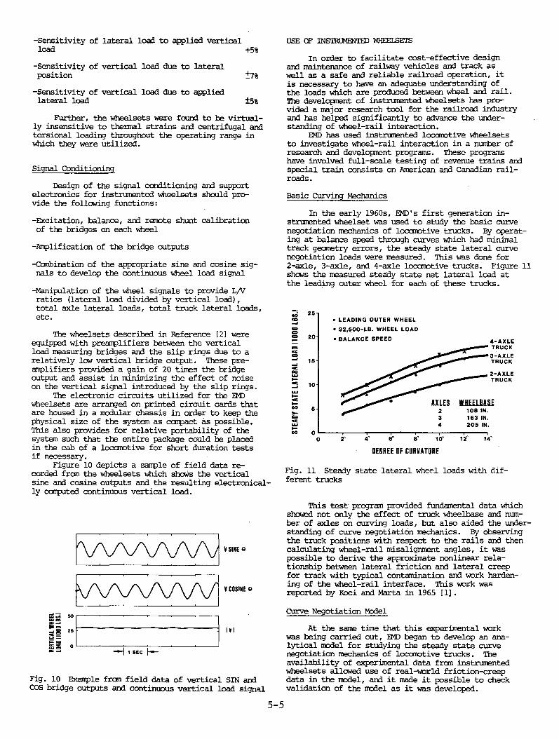
-Sensitivity of lateral load to applied vertical load +5%

-Sensitivity of vertical load due to lateral position ±7%

-Sensitivity of vertical load due to applied lateral load ±5%

Further, the wheel sets were found to be virtually insensitive to thermal strains and centrifugal and torsional loading throughout the operating range in which they were utilized.

Signal Conditioning

Design of the signal conditioning and support electronics for instrumented wheelsets should provide the following functions:

-Excitation, balance, and remote shunt calibration of the bridges on each wheel

-Amplification of the bridge outputs

-Combination of the appropriate sine and cosine signals to develop the continuous wheel load signal

-Manipulation of the wheel signals to provide L/V ratios (lateral load divided by vertical load), total axle lateral loads, total truck lateral loads, etc.

The wheelsets described in Reference [2] were equipped with preamplifiers between the vertical load measuring bridges and the slip rings due to a relatively low vertical bridge output. These preamplifiers provided a gain of 20 times the bridge output and assist in minimizing the effect of noise on the vertical signal introduced by the slip rings.

The electronic circuits utilized for the EMD wheelsets are arranged on printed circuit cards that are housed in a modular chassis in order to keep the physical size of the system as compact as possible.This also provides for relative portability of the system such that the entire package could be placed in the cab of a locomotive for short duration tests if necessary.

Figure 10 depicts a sanple of field data recorded frcm the wheelsets which shews the vertical sine and cosine outputs and the resulting electronically computed continuous vertical load.

wwwv V SINE e

W W W V * COSINE e

so

2 5

0

III

Fig. 10 Example from field data of vertical SIN and COS bridge outputs and continuous vertical load signal

USE OF INSTRUMENTED WHEELSETS

In order to facilitate cost-effective design and maintenance of railway vehicles and track as well as a safe and reliable railroad operation, it is necessary to have an adequate understanding of the loads which are produced between wheel and rail. The development of instrumented wheelsets has provided a major research tool for the railroad industry and has helped significantly to advance the understanding of wheel-rail interaction.

EMD has used instrumented locomotive wheelsets to investigate wheel-rail interaction in a number of research and development programs. These programs have involved full-scale testing of revenue trains and special train consists on American and Canadian railroads.

Basic Curving Mechanics

In the early 1960s, EMD's first generation instrumented wheelset was used to study the basic curve negotiation mechanics of locomotive trucks. By operating at balance speed through curves which had minimal track geometry errors, the steady state lateral curve negotiation loads were measured. This was done for 2-axle, 3-axle, and 4-axle locomotive trucks. Figure 11 shews the measured steady state net lateral load at the leading outer wheel for each of these trucks.

Fig. 11 Steady state lateral wheel loads with different trucks

This test program provided fundamental data which showed not only the effect of truck wheelbase and number of axles on curving loads, but also aided the understanding of curve negotiation mechanics. By observing the truck positions wath respect to the rails and then calculating wheel-rail misalignment angles, it was possible to derive the approximate nonlinear relationship between lateral friction and lateral creep for track with typical contamination and work hardening of the wheel-rail interface. This work was reported by Koci and Marta in 1965 [1].

Curve Negotiation Model

At the same time that this experimental work was being carried out, EMD began to develop an analytical model for studying the steady state curve negotiation mechanics of locomotive trucks. The availability of experimental data frcm instrumented wheelsets allowed use of real-world friction-creep data in the model, and it made it pxossible to check validation of the model as it was developed.

5-5

The early development of the curve negotiation model was done by Koci and Marta [1]. Further model development and computer programming were done by Swenson and Smith, and this work was published in 1976 in a report of the AAR [3].

Train Operation

In the late 1960s, EMD's first generation wheelset was used to help study train handling procedures and other operating conditions which were thought to influence the derailment potential of freight trains. The results of several major tests shed new light on the influences of locomotive and train braking practices, the location of enpty and long overhang cars in trains, and the use of sand to increase wheel-rail friction. This work was summarized in 1971 by Koci and Marta [4].

locomotive Adhesion

Instrumented wheelsets have also played a role in EMD's research to investigate locomotive and truck weight shift and wheel-rail interaction during driving and braking. A series of field tests conducted in the 1970s concentrated on developing funda-. mental data on the relationship between longitudinal friction and creep at the wheel-rail interface. This work was reported in 1980 by Logston and Itami [5].

Dynamic Wheel-Rail Load Characterization

Analytical prediction of dynamic wheel-rail loads has been one of the greatest challenges facing railroad researchers. Significant progress has been made in developing mathematical models in recent years. However, the accuracy of model results depends on knowledge of the track system characteristics, and adequate data has not been available to describe the range of track conditions that exist. As a result,- one of the most significant contributions from instrumented wheelsets has been the experimental characterization of the dynamic loads between wheel and rail.

The basic output obtained frcm instrumented wheelsets is generally in the form of time histories of wheel-rail loads.. This data provides information on both magnitude and time duration of the loads.

EMD's field tests in the 1960s provided information on the magnitude of transient dynamic lateral loads as well as steady state lateral curving loads.As noted in 1971, maximum dynamic lateral loads in curves were measured on 2, 3, and 4-axle trucks to be 12,000-15,000 lbs. higher than the steady state loads [4].

Vehicle-Track Interaction

In the mid-1970s, the attention of the railroad industry wras turned to a number of "unexplained” derailments of passenger and freight trains. There wras a resurgence of field testing programs to investigate dynamic wheel-rail loads. Until this time, most tests with instrumented locomotive wheelsets had focussed primarily on the locomotive wheel loads, i.e., the vehicle response. New test programs were conducted which focussed on the track input and response together with the vehicle input and response, i.e., the vehicle-track interaction. EMD participated with various railroads and other organizations in a number of major tests that utilized instrumented locomotive wheelsets.

In 1976, controlled tests were run writh 6-axle passenger locomotives at track sites which were specifically selected because they generated high dynamic

lateral loads. These tests, which measured loads both with an instrumented wheelset and with instrumented track, were reported in 1976 by Klinke and Swenson [6] and were later used as a framework for discussing various aspects of wheel-rail loading [7] .

Figure 12 shews the upper bound of the dynamic lateral loads measured in these tests on a curve of approximately 2000 ft. radius or 3 degrees. The figure also shews the steady state lateral loads for this size curve. It can be seen that with the dynamic component, the maximum lateral load wras approximately three times the steady state level.

Fig. 12 Steady state and dynamic lateral wheel loads

Measurement of the unloaded track geometry at the test site shewed that the track input included alignment deviations with an average wavelength of about 100 ft. and a peak-to-peak amplitude of 1.25 in. superimposed on the curve.

In 1977, EMD's third generation instrumented locomotive wheelset and EMD's test car were used in two major test programs which were directed by the AAR and by the FRA. These programs investigated vehicle-track interaction associated wd±h 4-axle and 6-axle locomotives and adjacent cars in passenger trains.

In 1978, the fourth generation instrumented wheelsets with continuous lateral and vertical load measurement capability ware used by EMD to study the performance of prototype 4-axle locomotives with various suspension systems. TVjo instrumented wheelsets were used to provide complete instrumentation of a 2-axle truck. The testing on one railroad produced two examples of the insight that instrumented wheelset data can provide about wheel-rail interaction:

1. In an area of continuous welded rail and very good track quality, dynamic lateral loads up to 30,000 lbs., as shown in Figure 13, were measured in a 3 degree curve. Close examination of the time histories and inspection of the track shewed that the lateral load dropped nearly to zero at a repair joint in the outer rail and then increased to its maximum level about 5 ft. beyond the joint. At 60 itph, this change from zero load to maximum

5-6

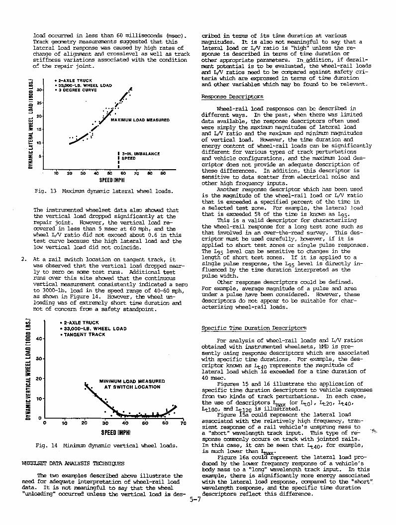
load occurred in less than 60 milliseconds (msec). Track geometry measurerents suggested that this lateral load response was caused by high rates of change of alignment and crosslevel as well as track stiffness variations associated with the condition of the repair joint.

The instrumented wheel set data also showed that the vertical load dropped significantly at the repair joint. However, the vertical load recovered in less than 5 msec at 60 mph, and the wheel L/V ratio did not exceed about 0.6 in this test curve because the high lateral load and the low vertical load did not coincide.

2. At a rail switch location on tangent track, it was observed that the vertical load dropped nearly to zero on seme test runs. Additional test runs over this site shewed that the continuous vertical measurement consistently indicated a zero to 3000-lb. load in the speed range of 40-60 mph, as shown in Figure 14. However, the wheel unloading was of extremely short time duration and not of concern frem a safety standpoint.

Fig. 14 Minimum dynamic vertical wheel loads.

WHEELSET DATA ANALYSIS TECHNIQUES

The two examples described above illustrate the need for adequate interpretation of wheel-rail load data. It is not meaningful to say that the wheel "unloading" occurred unless the vertical load is des

cribed in terms of its time duration at various magnitudes. It is also not meaningful to say that a lateral load or L/V ratio is "high" unless the response is described in terms of time duration or other appropriate parameters. In addition, if derailment potential is to be evaluated, the wheel-rail loads and L/V ratios need to be compared against safety criteria vhich are expressed in terms of time duration and other variables vhich may be found to be relevant.

Response Descriptors

Wheel-rail load responses can be described in different ways. In the past, when there was limited data available, the response descriptors often used were simply the maximum magnitudes of lateral load and L/V ratio and the maximum and minimum magnitudes of vertical load. However, the time duration and energy content of wheel-rail loads can be significantly different for various types of track perturbations and vehicle configurations, and the maximum load descriptor cbes not provide an adequate description of these differences. In addition, this descriptor is sensitive to data scatter from electrical noise and other high frequency inputs.

Another response descriptor vhich has been used is the magnitude of the wheel-rail load or L/V ratio that is exceeded a specified percent of the time in a selected test zone. For example, the lateral load that is exceeded 5% of the time is known as L95.

This is a valid descriptor for characterizing the wheel-rail response for a long test zone such as that involved in an over-the-road survey. This descriptor must be used carefully, however, if it is applied to short test zones or single pulse responses. The L95 level can be sensitive to Changes in the length of short test zones. If it is applied to a single pulse response, the L95 level is directly influenced by the tine duration interpreted as the pulse width.

Other response descriptors could be defined.For example, average magnitude of a pulse and area under a pulse have been considered. However, these descriptors do not appear to be suitable for characterizing wheel-rail loads.

Specific Time Duration Descriptors

For analysis of wheel-rail loads and L/V ratios obtained with instrumented wheelsets, EMD is presently using response descriptors which are associated with specific time durations. For example, the descriptor knewn as L ^ q represents the magnitude of lateral load which is exceeded for a time duration of 40 msec.

Figures 15 and 16 illustrate the application of specific time duration descriptors to vehicle responses fran two kinds of track perturbations. In each case, the use of descriptors 1 ^ (or I -g) , Lt-20' Lt40 >Ltl00» and 1^120 i-s illustrated.

Figure 15a could represent the lateral load associated with the relatively high frequency, transient response of a rail vehicle's unsprung mass to a "short" wavelength track input. This type of re- * sponse carmonly occurs on track with jointed rails.In this case, it can be seen that L ^ q , for example, is much lower than I^^.

Figure 16a could represent the lateral load produced by the lower frequency response of a vehicle's body mass to a "long" wavelength track input. In this example, there is significantly more energy associated with the lateral load response, compared to the "short" wavelength response, and the specific tine duration descriptors reflect this difference.

TIME TIME DURATION (MSEC)15a 15b

Fig. 15 Application of specific time duration descriptors to vehicle response fran "short" wavelength track perturbation

TIME TIME DURATION (MSEC)16a ' 16b

Fig. 16 Application of specific time duration descriptors to vehicle response fran "long" wavelength track perturbation

Figures 15b and 16b shew how specific time duration descriptors can be used to describe the relationship between lateral loads and the tine duration associated with each load level. Using this technique, the response can be characterized for the canplete range of time durations that is of interest.

Figure 17 shews a carp arisen of these hypothetical "short" and "long" wavelength responses.A number of vehicle performance criteria and derailment criteria have been expressed in terms of time durations at each response level, and use of specific time duration descriptors makes it possible to compare different vehicle responses to these criteria.

The actual wheel-rail load data shown in Figure 13 was analyzed by this technique. Sunmary curves are shown in Figure 18 for time durations of 0, 20, 40, and 100 msec. This type of plot provides insight into the level of dynamic load associated with various time durations at different vehicle speeds. In this example, the 100 msec level corresponds approximately with the steady state lateral curving load.

TIME DURATION IMSECI

Fig. 17 Comparison of vehicle responses to performance or derailment criteria5-8

Fig. 18 Effect of speed on time duration of dynamic lateral wheel loads

There appears to be a number of advantages in using specific time duration response descriptors:

1. While other descriptors provide only a single data point for each wheel-rail response or test zone considered, this technique provides a series of data points which account for the time duration of the response and attempt to reflect the energy content of the wheel-rail loads.

2. This technique may help to provide a framework for experimental development of better derailment criteria. Adequate derailment criteria, especially for rail rollover and track shift, are not yet available for the range of track conditions which exist in the real world.

3. This technique does not require ccmputer processing of the data. It can be done manually to provide quick, accurate, on-board data analysis, especially during site testing.

4. Real-world track conditions often produce multiple wheel-rail responses in a test zone, and this technique can be applied to complex as well as simple response waveforms.

HJTURE WHEEISET DEVELOPMENT AND USE

EMD continues to actively develop and use instrumented locomotive wheelsets. Currently, a fifth generation wheelset design is being built. As illustrated in Figure 19, this new vheelset will provide continuous measurement of axle torque developed at both wheels as well as continuous lateral and vertical wheel loads.

Improvements have been made regarding the lateral and vertical load output compared to the fourth generation vheelset described in Reference [2]. New equipment was used to provide more accurate numerical control machining of the wheel plates, which resulted in slightly higher sensitivity, better sinusoidal waveform uniformity, and reduced crosstalk. A new calibration fixture has been built to provide more accurate positioning and loading and more rapid calibration.

Plans are being made to use this new vheelset in two test programs in 1981: .

1. Three instrumented wheelsets will be used in a 3-axle truck for tracking and ride quality tests. Electronic processing is being developed to provide continuous signals of individual wheel L/V

Fig. 19 Fifth generation instrumented vheelset

ratios and IL/EV ratios for each truck side as well as individual lateral and vertical loads.

2. Instrumented wheelsets with torque measuring capability wall be used in EMD's continuing adhesion research program to develop friction-creep curves for individual wheels. The wheelsets will be used simultaneously to investigate the phenomenon of torsional vheelset vibrations.

ACKNOWLEDGEMENT

Many present and former members of EMD’s Analytical, Experimental Test, Instrumentation, and Truck Design Groups have contributed to -the development of EMD's instrumented wheelsets. A number of railroads have assisted by providing the use of locomotives, test sites and other support.

REFERENCES

1. Koci, L.F. and Marta, H.A., "Lateral Loading Between Locomotive Truck Wheels and Rail Due to Curve Negotiation," ASME Paper No. 65-WA/RR-4, 1965.

2. Modransky, J., Donnelly, W.J., Novak, S.P., and Smith, K.R., "Instrumented locomotive Wheels for Continuous Measurements of Vertical and Lateral loads,"ASME Paper No. 79-RT-8, 1979.

3. Smith, K.R., MacMillan, R.D., and Martin, G.C., "Technical Documentation of 2, 3, and 4 Axle Rigid Truck Curve Negotiation Model," Association of American Railroads/Track Train Dynamics Report No. R-206,1976.

4. Kdci, L.F. and Marta, H.A., "Wheel and Rail Loadings from Diesel Locomotives," Proceedings of the 70th Annual Convention of the AREA, Vol. 72, 1971.

5. Logston, C.F., Jr. and Itami, G.S., "Locomotive Friction-Creep Studies," ASME Paper No. 80-RT-l, 1980.

6. Klinke, W.R. and Swenson, C.A., "Tracking and Ride Performance Of Electro-Motive Six-Axle Locomotives," Technical Proceedings of 13th Annual Railroad Engineering Conference, Pueblo, Colorado, 1976, FRA/ORD Report No. 77/13.

7. Koci, H.H. and Swenson, C.A., "Locomotive Wheel- Rail loading - A Systems Approach," Proceedings of the Heavy Haul Railways Conference, Perth, Australia, 1978.

5-9

DISCUSSION

Mr. Caldwell: Caldwell from CN Rail. In your load measuring bridgefor lateral, the $ine/cosine techniques for the lateral bridge, how do you determine the sign of the load? Is there auxiliary instrumentation of the position or angle?

Mr. Smith (EMD); We're working with absolute magnitude of the lateral load and your question on is how do you get the sign, the plus or minus sign, for the lateral load. We wrestled with that problem for quite some time and for a while, we had a gauge on the wheel which provided us, we thought about putting a gauge on the wheel to tell us which direction the sign was, and eventually, after quite a bit of review, we opted to just go with the magnitude of the maximum lateral load and not worry too much about the direction of it. The reason is that in the applications we foresaw for that particular wheelset, the direction of the sign was not critical to us. It is a point, it is something that we are working with. We've got some circuits that are worked up in this fifth generation wheelset that Curt described which essentially used a position indicating device on the wheel to extract the sign.

Mr. Zuck (DB): Did you determine the conformity error for the sine andcosine?

Mr. Smith: Yes. I think that the slide that we had up there lookedsomething like the sine and cosine wave. We actually overlaid a sine wave and cosine wave, a raw sine and cosine wave, and we found that throughout the whole rotation, that + 5 percent was the accuracy of the wave with the sine and cosine. I might add that the maximum disagreement that we had was really due to lateral position on the vertical bridges. We were probably down to 2 or 3 percent on just the lateral load measuring bridges.The vertical bridges were about + 5 to 6.

Mr. Swenson: The uniformity of the sine and cosine waves is evenbetter for the fifth generation. We didn't show any pictures of that.

Mr. Brantman: Russ Brantman, TSC. Karl, did you have any problemswith temperature or centrifugal compensation?

Mr. Smith: We did on the first wheelset, the one we made in 1962.We had a terrible time with temperature, and with the 1972 wheelset that we talked about, the second generation wheelset, we were able to cancel thermal strains and centrifugal effects that are generally symmetrical on the wheel plate. The strains distribute themselves in a symmetrical fashion. We chose gauge locations and wired them on the bridge such that any centrifugal strain, regardless of where it came from, would be automatically cancelled in the bridge, and we were just looking at the variable strain due to the applied lateral load which gives you kind of a cosine strain distribution through the wheelplate. Anything that's symmetrically distributed through the wheelplate such as centrifugal effects or the thermal effects cancel out of this bridge.

5-10

TAGE J. ANDERSONChief eng., Research and Development Rolling Stock Department Swedish State Railways STOCKHOLMJanuary, 1981.

Calibration guidelines and equipments, important characteristics and error types for instrumented wheelsets

Summary:

This paper is an attempt to create better possibilities for design, calibration and comparison of instrumented wheelsets. Therefore, important characteristics and error types for instrumented wheelsets are listed and a comprehensive guide how to establish those characteristics and errors is given.Also calibration equipments, used by Swedish State Railways, are briefly described.

6-1

Calibration guidelines and equipments, important characte

ristics and error types for instrumented wheelset.s.

1. Calibration guidelines1.1 Necessity for calibration1.2 Field calibration1.3 Laboratory calibration

2. Important characteristics and error types for instrumented wheelsets

2.1 Measuring principle2.2 Sensitivity2.3 Stability2. b Drift2.5 Ripple2.6 Contact point lateral position influence2.7 Y-magnitude influence2.8 Torque influence2.9 Speed influence2.10 Reproducibility2.11 Linearity error2.12 Transfer function2.13 How do we determine these characteristics?

3. Calibration equipments or rigs, used by SJ

3.1 Static test rig3.2 Dynamic test rig3.3 Features and drawbacks of the two test rigs

6-2

Figures

Fig. 1 " 2

" 3" k

" 5

" 6

" 7" 8

" 9" 10

" 11 " 12

" ' 13 " Hi

Y-force check Field Equipment Continuous measurement Discontinuous "Def. of Sensitivity, Reproducibility and LinearityDef. of Stability and DriftDef. of Undulation and Anomaly (Ripple)Contact point PositionStatic calibration test rig, overall view Measurement of Y and Q in static test rig Contact point arrangement Dynamic calibration test rig,

M If 3II It

11 It

1! M

M M

overall view clamping arrangement driving "rollers

6-3

Calibration guidelines and equipments, important characteristicsand error types for instrumented wheelsets

1. Calibration guidelines

1.1 Necessity for calibration.

It is of prime importance to know the limits of error for any measuring device. For instrumented vheelsets (IW., or measuring wheelsets) this surely is true, because of the number and magnitude of unwanted, influencing factors. To measure a vertical force wheel/rail of a magnitude 1 kN with a typical I.W. we utilize a medium strain change in the strain gauges on the wheel plate of about 0,o2 fjoni/m. At the same time we have many .other factors causing strains in the wheel plate, some of them with the magnitude hundreds of pm/m. We would not be able to make a correct choice of position for and coupling of the strain gauges, that is to produce a good I.W., if we could not apply exactly known forces at given positions on the wheel.

For this reason we need to perform laboratory calibrations.Field calibrations serve as a function control during field applications.

1.2 Field calibrationField calibrations of the Y- and Q-forces are necessary to ensure a proper function of the measuring chain.

By means of hydraulic jacks under the journal boxes we lift the I.W. (and so the wagon) to secure that no force wheel/rail is present. We now can establish and record the datum line for both Y- and Q-force.The simple equipment in fig. 1 can now be applied between marked spots on the gauge side of the Vheel flanges. By means of the built-in hydraulic jack and force-transducer we now can apply a suitable calibration Y-force. This force is of opposite direction to usual Y-forces. Laboratory checks of the strain sensitivity for both directions will as a rule show that they are equal.An approximative, but for many purposes acceptable, reference line for Y- and Q-forces can be established by recording Y and Q at low speed on straight track. The so recorded Q-force should be approximately equal to the static wheel load Qq (the sum of the recorded left and right hand vertical forces equal to the axleload 2-Qq ). The recorded'Y-force should be approximately equal t° Qo’ A , where X = conicity angle of the wheel thread.

6-4

Goals for the laboratory calibration are to specify important characteristics and limit values of errors for the I.W.Studying derailment phenomena, wear or riding properties we want to know the forces in the contact areas wheel/rail. Maybe we want to treat the measured values of these forces differently depending on the main aspect in our investigation - but mostly we must know the true forces in the contact areas. If we investigate for wheel shaft fatigue we surely have another aspect than if we want to calculate the climbing action of the wheel on the rail.With various measuring methods we measure the remains of these contact forces, at different places according to the measuring method (in the wheel plate, in the spokes or in the wheel shaft). Therefore, it is essential to know the transfer function between the contact areas and the measuring spot. Up till now, very little such knowledge exist.The measuring accuracy of a measuring wheelset can be verified by dynamic, and to some extent, static tests. Here we define dynamic test as a test where the wheelset is rolling during the calibration procedure.It is recommended to use the static nominal load Qq as decisive guiding value for Y and Q. In this way the extent of these tests can be limited and the percentage of error can be referred to one and the same value. In order to arrive at. a simple comparison of various measuring wheelsets, it should be endeavoured to apply the guiding value Qq = 100 kN.Now I will designate the decisive magnitudes for the assessment of measuring inaccuracy for the Q-force measuring system of a measuring wheelset. A very similar procedure must be applied for all measuring systems (Y, Q and Tx) and may result in a scheme like Table I.In order to be independent of amplifier feeding voltages, I have chosen to express the errors in (virtual) strain or inspecific (virtual) strain jum/nr/kNj. Note that tiese strain values are medium virtual strains for the whole measuring bridge, not the maximum strain in a specific strain gauge.

As strain and force (in kN) are related through it is then easy to compare errors and true Q-signal.

All the following error factors 2.3 - 2.11 can be expressed as absolute or relative errors. The absolute errors should be expressed in kN'or jrni/m (note that errors in category 2.3, 2.b, 2.9 can be expressed in kN with the knowledge of X2 for a specific measuring wheelset) and the relative errors should always be related to the reference value 100 kN. Some of the errors (XJ4 and X9) have not been expressed in relation to the free variable, which usually brings advantages in other cases. In these cases, there are nonlinearities, reducing the merit of this procedure.

1.3 Laboratory calibration

6-5

Important characteristics and error types for an I.W.

Measuring principle for Q

Define measuring system as continuous or discontinuous and in the latter case state measuring interval and length. This definition is of decisive importance for the measuring inaccuracy.

Sensitivity for Q (Y=0) .... X2 jim/m/kN.The sensitivity is defined as the mean value for the force range 10-100 kW. The choice of another force range may effect the errors 2 .10 and 2 .1 1 .

Stability error of measuring system .... Xg jcn/mPure temperature influence, attributed to homogenous, gradual variations in ambient temperature or to braking action. Most measuring wheelsets cannot accept braking action because of the great error caused by the temperature gradients by braking.

Recommended value At = 20° in the temperature range 0 - 20°.

Drift in practical operation .... Xl; jim/m.

Dominated by temperature gradients in wheel disc (caused by rolling resistance in axle bearing and at contact points), cooling, driving and loading conditions and intervals, wheather conditions and so on. Also includes drift in other parts (signal transmitter wheel-journal box, cables, amplifiers and so on) of the measuring chain.

Specify maximum error for given practical test conditions.

Ripple: undulation and anomaliesat Q = Qo . . . . X5 jim/m/kN.The undulation is here defined as the amplitude of the periodical deviation, the anomaly as the maximum amplitude of the nonperiodical deviation from the constant 100 kW-output signal.If there is an Y-influence on Q, the Y-value may influence upon X^ Then at Q = Qq , Y = Qq kN .... X5 Q^Jim/m/kN.

Contact point lateral position influence .... XgjXX jim/m/kN.The lateral distance from the Running Circle to the point of Q application is designated by xx (y-distance from Running Circle) as a second index for Xg (Xg xx)• This error is measured at Y = 0 Q = 100 kN and for positions’xx as 00, -10, -20 mm. If the wheelset is to be used for derailment investigations, extrapolation can be used to calculate Xg 3 5, for a Q-position near the flange (35 mm from the Running’circle).

6-6

2.7

2.8

2.9

2.10

2.11

2.12

2.13

This influence is measured (at Q = 0) for Y =.100 kU.Y-magnitude influence .... Xj n/m/kK.

Torque influence .... Xg jim/m/kNm.Most measuring wheelsets are sensible to traction or braking torque because of the temperature effect, see error category U But here we state the sensitivity to the torque as such, which always exists in variable magnitude at normal running. Torque influence is measured at a torque of 25 kNm.

Speed influence .... X^ jim/m.

Influence of centrifugal forces in the wheel plate, measured at Y and Q = 0.

This error can be compensated with a function generator. The influence is non-linear and must be measured up to expected test speeds. For sake of comparison, state error at speed 100 km/h:X9 ,loo P m /m -

Reproducibility error .... Xqg Jim/in/kN.

The Q-reproducibility X - J q for each of the force steps (10 calibration force steps of 10 kN each, from 0-100 kN) is defined here as the standard deviation of the measured values for one and the same force magnitude.The Q-range reproducibility Xln for the total Q-range including all the force steps is here defined as the variation range for the standard deviation for all force steps.

Linearity error .... Xqq jim/m/kN.

The linearity error is here defined as the maximum deviation between the mean values for each force step and the mean value relating to the overall range of forces.Experience tells this is a minor error.

Transfer function .... X-^*This transfer function (contact area/measuring spot) can be evaluated for all forc&*(Y, Q and Tx) directions by applying dynamic pulsators in the contact areas or at the wheel rim.

How do we determine these characteristics?Naturally everybody tries to eliminate and reduce as many errors as possible already during the design of the measuring arrangement (i.W. + signal conditioning) and also by an appropriate choice of the test procedure and conditions. For now existing

6-7

measuring wheelsets, the greatest errors are to be expected for the factors of type 2.k - 2.8. The/2.10 and 2.11 may play quitean unimportant role. /factorsCharacteristic No. 2.2 (Sensitivity) can be established by static as well as dynamic tests. The accuracy of this characteristic may even depend on the design of the static and dynamic test rigs.The error of type 2.3 (Stability) aims at field conditions but may be simulated through exhibiting the non-loaded I.W. to different environmental temperature and also on a dynamic test rig by symmetric heating on the axle near the journal boxes and on the wheel thread. Other values than those recommended here can be used when field studies have demonstrated need therefore. Error type 2.U (Drift) has to be determined for given field conditions. Eventually can loading conditions be simulated in an advanced dynamic test rig.

Error type 2.5 and 2.9 haveto be determined in a dynamic test rig. Error type 2.6, 2.7, 2.10 and 2.11 can be determined in static or dynamic test rigs.

Error type 2.8 is easily determined in a static test rig.

3• Calibration equipments or rigs, used by SJ.

The calibration equipment for field use is already mentioned under point 1 .2 .

\

For laboratory calibration SJ uses two test rigs, one of static type, the other of dynamic type.

3.1 Static test rig

Figure 8 shows the static test rig. The I.W. is placed upon two short rail beams, one under each wheel. One rail is mounted on a measuring device which by means of four measuring bolts is fixed to the rig frame. The measuring bolts separately measures vertical and lateral forces, existing between wheel/rail. (See RP 11, ORE B 10: BR type of measuring chair) and fig. 9 .Vertical forces are applied with vertical hydraulic jacks between the rig frame and journal boxes.Lateral force is applied with another jack between rig frame and field side of wheel rim. Two hydraulic jacks can be activated to lift the wheelset from the rails, in order to rotate the wheel.To establish a precise contact point (area) wheel/rail we use a steel cylinder between wheel and rail, see fig.1 0 .The rig can be used for railway wheels of any wheel diameter.

6-8

The accuracy of this static test rig is mainly determined by the measuring bolts. Vertical force is measured with a sensitivity of 12,36 jim/m/kW with a max. error of -1%, in measuring range 10-100 kN. Lateral force is measured with a sensitivity of 80,5 jxm/m/kN and with a max. error of *1,5%, in measuring range 10~50 kN.There is a certain cross-influence between vertical and lateral force. For a vertical force Q = 100 kN (Y=0) the lateral transducer indicate a lateral force of 0,31 kN, when Q is positioned on the running circle. Since this lateral force always is measured by the measuring bolts there is no real problem.In the case of a combination of Y- and Q-forces applied on the wheel thread, the quotient Y/Q cannot be higher than the dry friction value, i.e. about 0,U. For a contact point on the flange higher quotient- (and so Y-) values can be utilized.

3.2 Dynamic test rig.

Fig. 11 shows the dynamic test rig. The I.W. is clamped to the rig frame (fig. 12 ) by means of for the purpose designed "journal boxes",., at each such journal box. The wheelset rotates, driven via cardan shafts (fig. 13 ) and a mechanical change gear (at one axle-end) of an electrical motor. The iakExai maximum speed is 120 km/h at no load. Vertical and lateral forces are applied through two pair of rollers (fig. lU ) at each wheel. These rollers are actuated by hydraulic jacks, supplied through regulators from a hydraulic pump. Application range for Y- and Q-forces are 0-150 kN and 0-200 kN respectively.

3.3 Features and drawbacks of the two test rigs.The static test rig features the better accuracy. The accuracy for the dynamic rig is dependent of constructional accuracy for the I.W. If (which always seems to be the case) the wheel threads of the I.W. show out-of-roundness and/or skew (lateral), these mechanical inaccuracies add undulations and anomalies to the applied constant Q- and Y-forces. To limit these effects we have introduced pneumatic accumulators in series with the hydraulic media. But we still have to claim for wheels with very good mechanical/geometric dimensions.Dry friction in the lateral roller's guidance system is another drawback for the dynamic rig. So is friction in the hydraulic jacks behind the vertical and lateral rollers. For a mechanic/ /geometric ideal wheel in the above sense the accuracy would be of the same magnitude as for the static rig.Measurements in the static rig are very time-consuming. The dynamic rig can automatically deliver an immediate record of Y or Q, alt. Tx as a function of rotation angle and is hence very time-saving.To determine errors type 2.5 and 2.9> a dynamic test rig is more or less a must, as already stated under point 2.12.

6-9

At the calibrations there are some difficulties caused by the inclination of the wheel thread. An approach to meet this is to calibrate the wheelset with cylindrical wheel thread and after the calibration reprofile the wheels with actual profile. This approach can be accepted when the reprofiling does not change the pattern of strain in the wheel plate.

The dynamic rig could surely he of more sophisticated design.

6-10

Table 1

Important characteristics and error types for an I.W.

Y-measuringsystem

Q-measuringsystem

----------- --- 1T -measuring

system

1. Measuring principle X X X X xxxx xxxx

2. Sensitivity xxxx xxxx X X X X X

3. Stability X X X X X X

. Dri ft X X X X X X

5- Ripple X X X X X X

6. Q-position influence X X X X X X

7. Y-influence - X X X X |

8. Torque influence X X X X1

9. Speed influence X X X X X X |1

10. Reproducibility X X X X1

X X

11. Linearity X X X X X X

12. Transfer function X X X X X X

6-11

6-12

Fig.

£1-9

Z *3M

, 0 £ Z , 0 8 1 , 0 6

J .N 3 N 3 V3M S/7 O N U N O ?

CONTINUITY..,- D L E IM IIO N S

OVERLAPPING QhMEIHQD„..(LLDERLY aPQKE-MHEEL LtTHQDI

CONFIGURATION FOR MEASURINGBRIDGES.! M3J1

Mensur ing M ER VALS:Qy : W°- 140° AND 220° - 320° (ANOMALY-22 %)

02 : m ° - 220° AND 320° - 40° ( )

Fig. 3

6-14

o /\

DEFINITIONS OF THE CONCEPTS, SENSITIVITY, LINEARITY AND REPRODUCIBILITY ERROR

BfflilLFOR Q ffASURFMFNT. Y = 0

STRAINS PER kN Pm /m /kN

Fig. 9a

6-21

Y

Q

t « Ttmptratur- Komptruation

*

t l E A 5 7 / 7 T E K E N T

o f ^ / — Q - jcscC'S

in S -ia+ ic i~es-& ricf

6 - 2 2

DISCUSSION

Mr. Johnson (IITRI) : Fo'r your lateral load on the dynamic calibrator,is that applied on the side of the rim?

Mr. Anderson: Yes, on the outer side of the rim. But if you check withyour wheels, I think you should draw the same conclusions as we did, that the direction from outside and in is the same sensitivity as from the opposite direction. So there seems to be equality.

6-25 / 6 - 2 6

DETERMINATION OF WHEEL/RAIL FORCES BY MEANS OF MEASURING WHEELSETS ON

DEUTSCHE BUNDESBAHN (DB)

Heinz-Herbert Ztick

Bundesbahn-Versuchsanstalt PionierstraBe 10

4 950 Minden (Westfalen)

1. INTRODUCTIONThe interaction between vehicle and track and, to a sp ec ific degree, the forces occurring at the wheel/ r a i l contact point have a fundamental bearing upon the running sa fety and rid ing qu a lity o f railway veh ic les , as w e ll as on the stress and wear imposed on running gears and permanent way. Higher operating speeds and greater axle loads are due to be implemented fo r commercial reasons, and i t is therefore absolutely e ssen tia l to obtain a be tte r understanding of the e ffe c ts upon the vehicle and the permanent way due to these requirements. To determine the mechanical stresses upon the permanent way i t is not su ffic ien t to measure these forces re la t iv e ly . On the contrary, these fundamental investigations necessitate knowing the absolute value o f those forces occurring at the contact point between wheel and r a i l . Because o f the complexity involved, measurements at fixed track locations have to be lim ited to a few meters only, and the forces should therefore be defined via the veh icle. I t is notable that any vehicle at a l l , together with it s appertaining and even most varying types o f wheelsets and powering equipment, may in p rin c ip le be used as an object fo r determining such forces without f i r s t having to produce a specia l wheel fo r th is purpose. Deutsche Bundesbahn (DB) are currently employing measuring wheelsets which enable the forces occurring at the w heel/rail contact point to be measured v e rt ic a lly , horizon ta lly and in the d irection o f t ra v e l simultaneously and continuously. The fo llow ing paper is intended to e lucidate the theory o f such a "measuring wheelset" and to d iscribe the ca lib ration process and the characteristics of the measuring procedure o f the so -c a lled "Wheelset-Axle-Method".

7-1

2. THEORETICAL FOUNDATIONSThe test method is based on the fact that external forces a ffec tin g the wheelset produce a bending moment upon the ax le . From the bending moments measured in w elldefined cross-sections the external forces can be determined. F ig . 1 shows a wheelset with r e a lis t ic assumptions o f these forces.Y, Q, T are measured values, which by the te st method are indicated at the contact points A^ andFr and FR 2 resu lt from t i l t in g o f the axleboxes andproduce an additional bending moment upon the wheelset. With FD and F ^ we consider forces which are createdby hydraulic damping elements. The bending moments in the ind iv idual cross-sections are computed in the Y - Z plane defined by the v e rt ic a l and horizontal forces and shown in the system o f equations 1.

MelJquerschnitt A

•Ayi Al ' WA ~~ f~D lh,.

MelJquerschnitt B

^Byi ~ Oft ' Wg = Fqi (bjy - b j ) + FKit • ay + Fa •■ (/>,! - bj) .

Mefiquerschnitt C

Mc * = 0 & ■ Wc = Fox (torf -63) + F k u •*, + (to,, -63) + Q, u»AX -63) - • r,

= Fd 2 ibd2 + 63) + FK 2i ' <*2 + F ,2 (to,2 f *3) + Q2 lb*? + £>3) + Y2 • r2.

MelJquerschnitt D

M0yj = n0t ■ W0 - FpX (b ^ + to4) + Fk u ■ B\ + Fry (to,, + to«) + Q, (fc„, + to«) — K, ■ r<

- Fq 2 (torf2 - to4) + F m ■ »2 + Fx2 (to, 2 - to4) + Q 7 (b A2 — to4) + y2 ■ r7

MelJquerschnitt E

M t * - <r& • W e - F p i {bd2 - toj) + Fk 2 , ■ a2 s- Fn (to,2 - to5).

7-2

MeBquerschnitt f

M Fy! - af, ■ Wf — Fq2 (bdi — t>i) + Fkii • ®3 + {bn — bg)

S Y S 1

The equations fo r the bending moments o f the c ross- sections in the plane defined by the horizontal and tangential forces, which are used for determining the Tx forces, are equivalent to the equations o f theY - Z plane. In setting up the equations i t must be borne in mind that the la te ra l forces F^ o f the ax le -boxes have zero -levering e f fo r t and that in the x - direction there are no forces due to damping elements,i . e. Y = Y 2 = FD = FQ 2 = 0. In addition andmust be substituted by Tx and T 2 and index z by x.We then obtain the forces Y^, Y2 , 0^, Q j r Tx and TX 2

acting upon the wheelset by measuring the bending moments in the cross-sections A - F a fte r having su itab ly transformed the equation system 1.

. . bA , + b* bA} - b ilb, (ft, - ft,! ' (ft3+ft4),, + (£7bJ7r

b z - b d'A2lb$ - be,) tj ■M, b* - b A2 mm b A7 + b j f t -

Maft, ftj'ft, -ftj Mb" ftTTft/ Mc» A^TftTM°v’

q 2 ^ - 7-----r— M,oc-fti fte-fts b2 VbA M °yi + ft +ftj M,C y i

7-3

6i - t>2 ■MAlA r yt i i - b 2

Me,6 3 + 6 4

■M,Cxy 63 i b t-M,'D xy

T„, -h-b* M,Exy

___J__63 + 64 %- ' + V + 64

’Me.

S Y S 2

The Wheelset Axle Method determines the bending moment by considering Hooke's Law d ire c t ly from the deflection o f the wheelset at the predetermined p o s it io n .

c 4 - M 'w E " E E

( 1)

The deflection at a cross-section is measured in the X - Y and the Y - Z planes by the a lte ra tion of resistance in a Wheatstonebridge c ircu it consisting of stra in gauges coupled as shown in F ig . 2 (equation 2) .

A RR

= K'£ (2)

By assuming that the forces acting in the Y - Z plane generate a lterations o f resistance A rz ( ARX = 0)and that the forces acting in the X - Y plane generate a ltera tion s of resistance A R X ( ARZ = 0) the unbalanced voltages UDI and UDII o f both bridges are given

by equation 3.

7-4

COS K

)) ( 3 J

Considering the preceding equations, the bending moments in both planes are obtained by the follow ing eguation .

Equation 4 is the transformation o f the measured values from a coordinate-system which moves with the ro tating wheel in to a coordinate-system moving tangen tia lly to the tra in . The analogous switching o f the s ign a ls is done by means o f a computer as shown in P ic . 3. The computer outputs indicate the voltages fo r the Y, Q, Tx forces acting between wheel and r a i l .

3. STATIC CALIBRATIONThe fact that the constant K in equation 2 is subject to manufacture tolerances o f the stra in gauges necessitates the ca libration o f the measuring wheelset.

The wheelset is placed on two t ro lle y s , as shown in F ig . 4, which permits the wheelset to be turned in to any angular p o s it io n . The wheelset is suspended at theangular positions 0°, 90°, 180°, 270° and 360° at it s force attacking points A and A by hydraulic jackswith top-mounted force measuring c e l ls . The forces F^k and F3k caused by the wheelset weight attack atpoints A^ and A4 through self-made semi-annular rings.At the gauge side of each wheel d isc there are at in te rv a l A^ four p rec ise ly defined measuring points.The wheelset remains suspended while c a lib ra t in g the inside c ross-sections. The forces F2R are induced

My‘ ^ K UB {U° ' coiK ‘ Uo « ■ s i n * I

~ % , , ’ ( ^ o i ' s in /c + U0 „ • c o s k ).

7 - 5

at points and by an hydraulic jack v ia a barwith a mounted force measuring c e l l . The fo llow ing relationship ex ists between the bending moments and the induced forces.

MeBquerschnitt A

F,„W*

°A,

MeBquerschnitt B

M,c - "n* - °bia7 a2

MeBquerschnitt C

Mc,v _ Wc

MeBquerschnitt D

Moa 3

r- mOxy WD*?k = = "Ox

MeBquerschnitt E

F*Me We— = -----oE , .a4 tz

MeBquerschnitt F

MFy! WE— — = — Of,

S Y S 3

By turning the wheelset at 90° the other bridge c ircu its can be ca lib ra ted by the same method. The wheelset, ca lib ra ted in this way and having regard fo r it s sta tic tare-w eight is mounted under the test vehicle. The wheelset i s checked p r io r to commencement of actual f ie ld measurements on a specia l test r ig , which permits the simulation o f the Y and T^ forcesvia a c ro s s -ro l le r -c a r r ia g e , Q is simulated by loading and o ff-lo ad in g the te st vehicle (P ic . 5 ).

7-6

4. DYNAMIC CALIBRATIONAs the amplitudes o f the forces are time-dependant and because quantitative resu lts are required beyond the s ta t ic case, i t is a lso necessary to ca lib ra te the te s t method dynamically. The wheelset, securely mounted by it s axle-boxes upon a te st r ig , is jogged by an electrodynamical pu lsator which induces the Y and Q forces in the manner shown in F ig. 6. The c a l i bration o f the Tx” forces was impossible due to mechan ic a l reasons. F ig. 7 shows the block diagramm o f the evaluating cascade. The s ign a l from the wheelset computer is compared with the signa l from a quartz force transducer mounted on top o f the e le c tro dynamical pu lsator. The tran sfer function, with the amplitudes ra tio and the phase d ifferences and the coherence function as an ind icato r for the qu a lity of the te st are computed and p lo tted in the range from 5 Hz to 100 Hz as in Figs. 8 and 9. The accuracy fo r the Q -force is be tte r than 1 % in the range up to 25 Hz and be tte r than 5 % up to 30 Hz . A point of resonance occurs at 77 Hz.The accuracy fo r the Y force is be tte r than 1 % up to 22 Hz , a point o f resonance being found at 92 Hz.

5. ERROR EVALUATIONa) Mechanical e ffec tsIn the equation system 1 we have in the determinationo f the Y forces the levering e ffo r ts b_, and b„„A1 A2defined as constant parameters. But during the actual vehicle run th is assumption is no longer correct due to the change o f w heel/rail contact point and we thus have a measuring e rro r. Computing the la rgest absolute e rro r and assuming the remaining parts o f the system to be correct, we can obtain an estimation o f the in fluence o f th is e ffe c t upon the accuracy o f the Y forces. Thus equation 5.

10,1I = \hbA y\ • -p | —

IQz*lAVjl = 1 2 1 -77-(5)

7-7

I t is now c lea r that by changing the w heel/rail contact point we get an e rro r , which depends on the corresponding v e rt ic a l Q force and the radius of the wheel d isc . Where in curve negotiations a change of the w heel/rail contact po in t o f about 0.02 m occurs, we then get an in fluence upon the accuracy o f the Y force of about 4 % o f the Q force fo r a wheel d isc having 0.5 rad ius.

b) E le c t r ic a l e ffe c tsThe e le c t r ic a l e rro r is caused by the measuring cascade, which generates an e le c t r ic a l s ign a l from the mechanical deflection corresponding to the bending moments. A computation fo r the e rro r o f the bending moments is possib le under the assumption that the power supply to the bridge U0 , the factor

generate an e rro r , the la rgest re la t iv e e rro r such as in equation 6 .

mit Um ■ lime + UDn • com*0 .

The f i r s t two expressions are n eg leg ib le , because the e rro r o f the power supply is kept down with l i t t l e e f fo r t to less than 1 °/oo and the deviations o f the mechanical values are ca lib ra ted fo r each bridge c irc u it . The remaining re la tiv e errors o f the products between unbalanced voltages and sin and cos o f the wheel ro tational angle are given by the conformity e rro r o f the angular probe and by the e rro r o f the analogous m u ltip lie r. To minimise th is in fluence, angular potentiometers with conformity e rro r less than 0.5 % and m u ltip lie rs with an e rro r less than0.15 % are used. Additionaly the m u ltip lie rs with simular errors are se lected with the a id o f a d ig it a l computer and, based on the resu lts obtained,

and transformation portion o f the equation 4

mit UDI • c o m - l/0N • fin* * 0 (6)

7-8

incorporated into the measuring cascade fo r further e rro r suppression. The small unbalanced voltages (0 - + 5 mV) are pream plified by an am plifie r with high common mode rejection (120 dB) which is mounted on the axle as shown in P ic . 10, at which position there is no noise-interference on the measuring signals, at the same time requiring only a very simple zero adjustment fo r the measuring procedure. P ic . 11 shows the p ream p lifie r and angular probe mounted on the axle jou rna l.

c) Total e rro rThe to ta l e rro r fo r the forces is determined by the e rro r o f the e lec tron ica l equipment i t s value being less than 1 % fo r a l l forces except fo r the Y force, where we have an additional e rro r due to mechanical in fluence, which can override the e rro r caused by the e lec tron ica l equipment by a lte rin g the w hee l/ ra il contact point during tigh t curve negotiations.

6. SPECIAL FEATURESThe c lear mechanical theory o f the test method a lso allows it s application to very complicated wheelsets such as powered or braked wheelsets. By appropriatly choosing the number and the positions o f the cross- sections i t is possib le with such wheelsets to determine the forces acting between r a i l and wheel without in fluences due to powering or braking moments. Therefore, on Deutsche Bundesbahn adhesion is measured on braked wheelsets in accordance with the fo llow ing equation :

M »

7-9

The influence o f the varying w h ee l/ ra il contact point and i t s e ffe c t upon the Y forces enables us to obtain an absolute determination o f th is point as seen in equation 5. We are developing a te st method which permits the determination o f the horizontal forces by measuring tension and compression stresses . This method is independent o f the position of. the wheel/ r a i l contact point and, in conjunction with the Wheelset Axle Method makes i t possib le to carry out a coutinuous determination o f the respective contact- point position .

7. CONCLUSIONA measuring method was introduced, by means of which the forces occurring at the w h ee l/ ra il contact point in a l l three d irections may be determined simultaneously and continuously. With the exception o f the wheel contact-point e rro r relevant to the Y forces, the e rro r occurrence from the s t a t ic a l up to a spec if ie d frequency range is less than 1 %. The measuring method can be un iversa lly applied and has h itherto been employed on locomotives, powered multiple units, as w e ll as on passenger and fre igh t cars not only en Deutsche Bundesbahn (DB) , but also fo r mutual in vestigation work in collaboration with other railway adm inistrations.

7-10

*»dl *>di

Z

zTT

IZ

Fig. 2

IU JI

Fa02 OC/.CP

0 °

270°

Fa 02.007 CISm e im;wr-* •»

Fig. 6

7-14

Kraft m«(lscheib*n Kraftanlaitungsvorrichtung

Px Fx FxFy !■■■■! Fy l = ^ J FyFz Fz Fz

VLa dung s w«r s ter (rtf r

CHI

CH 2Auswcrttrcchrw

HP 5427 AD o tc n a u s -

g a b e

P / o t t t r

Radsatzrachner

Analogrtchner mit OMS-Varstarker

OHS - Aufnehmcr

7-15

VERSUCH 0 ANREGUNG UNGEREGELT KRAFT V, / KRAFT V„ F-.arw.TRANSFER FUNCTION

VERSUCH 0 ANREGUNG UNGEREGELT KRAFT V j / KRAFT M , F - . SHZ TRANSFER FUNCTION

DEG

VERSUCH 0 * ,Z O X * TRANSFER FUNCTION

7-16-

VERSUCH 3 OS ZU OR F-. 5HZ AVC-B4TRANSFER FUNCTION

10N

VERSUCH 3 OS ZU OR F -.5 H Z A V G -64 TRANSFER FUNCTIO N

DEC

VERSUCH 3 OS ZU OR F -.5 H Z A V C -64 TRANSFER FUNCTIO N

!■ ■ COHERENCE

7-17

PICTURE #3

J |F fVM W

| < 0 P L

». -i # '* ■ ®<J ® ' iiikl ■ '

l lM i i i * * * &gflf

. r , i T w i-te i |

f W ' ¥ l. M a r » ! • » ' « *

w® ■ Ie ® e ® 0 «# 4 "

S! fl

- . ' ' -lt_£i

7-18

PICTURE #5

7-19

PICTURE #10

7-20

PICTURE #11

7-21/7-22

SESSION 2: WHEEL/RAiL LOAD MEASUREMENT TECHNIQUES - I I

DEVELOPMENT AND EVALUATION OF WAYSIDE WHEEL/RAIL LOAD MEASUREMENT TECHNIQUES

Harold D. Harrison Donald R. Ahlbeck

BATTELLEColumbus Laboratories

505 King Avenue Columbus, Ohio 43201

Measurement of dynamic forces at the wheel/rail interface has long been of interest to railroad administrations, rail vehicle designers, and track designers. An accurate assessment of these forces is essential to the safe operation of trains, as well as the design of vehicle and track structural components. Techniques employed to measure wheel/rail forces fall into one of two categories: loads measured at a specific location in the track (way-side measurements) and loads measured at a specific rail vehicle (on-board measurements). In this paper, the development of wayside wheel/rail load measurement techniques and transducers is reviewed. An evaluation is presented of these different techniques based on recent laboratory experiments and field measurement experience, and a comparison is made of simultaneous measurements from current state-of-the-art wayside and wheelset load transducers.

INTRODUCTION

Loads at the wheel/rail interface are transmitted across a small contact patch on the running surface, except when the wheel flange contacts the rail, in which case a two-point load path exists. The forces at this interface are:

• Vertical forces due to the vehicle static weight, and dynamic forces due to irregularities on the wheel and rail running surface (wheel flats, rail joints, et cetera), the response of the vehicle to track geometry errors, and components of longitudinal train-action forces;

• Lateral forces from the vehicle response to track geometry irregularities, components of longitudinal train-action forces, external disturbances such as wind forces, self-excited hunting motions, and the creep and flanging forces necessary to guide the vehicle through curves;

• Longitudinal forces due to wheel-rail creep, traction (with powered wheelsets), and braking.

The force vectors at the wheel-rail interface are illustrated in Figure 1 for a typical loading situation, that of the lead outer wheel of a rail vehicle

8-1

Fv = VERTICAL LOAD AT TREAD CONTACT

Fy = VERTICAL LOAD AT FLANGE CONTACT

F, = LATERAL LOAD DUE TO CREEP FORCE LC (SHOWN FOR HIGH RAIL ON CURVE)

F]f = LATERAL LOAD DUE TO FLANGE FORCE

(LOADS SHOWN ACTING ON THE RAIL)

FIGURE 1.- SCHEMATIC DIAGRAM OF WHEEL-RAIL INTERFACE REGION

8-2

negotiating a sharp curve (radius of curvature less than about 1,000 ft). Wheel-rail loads have been characterized under typical revenue freight traffic^. Maximum expected load amplitudes from this source and from other experimental programs are summarized in Table 1 to provide an appreciation of the full-scale range required of wheel-rail load transducers.

HISTORICAL BACKGROUND

There are two different, yet fundamentally similar methods for measuring wheel/rail loads: with the instrumented wheelset, or with the instrumentedrail. Strain gages, in one case on the wheel plate or spokes, in the other case on the rail web or base, are used to transduce strains resulting from the wheel-rail loads into proportional electrical signals. Other methods have been employed in the past to measure wheel loads: combinations of load cellsand strain gages on the rail vehicle truck, or load-cell base plates beneath the rail, for example2. These methods are subject to substantial error in projecting the measured loads back to the actual wheel-rail loads. The current trend is toward direct measurement of loads at the wheel or rail.

Vertical Loads From Instrumented Rail

A variety of strain gage patterns have been applied to rail measurements of wheel-rail loads. Perhaps the most successful has been the vertical load measurement circuit adapted from strain gage patterns reported by the 0RE3>4.This pattern, illustrated in Figure 2, measures the net shear force differential between the two gaged regions, a-b and c-d. With the gage pattern placed between the rail support points (in the "crib", the space between crossties), the circuit output is directly proportional to the vertical load, P, as it passes between the gages. The influence zone of the pattern is very short, few inches either side of the mid-point between a-b and c-d, so that only a sample of short time duration is provided from each passing wheel. From laboratory and field tests, this pattern has shown excellent linearity and minimal sensitivity to lateral load (cross talk) or to the lateral position of the vertical load.

Other methods have been employed to extend the vertical measurement zone and provide a longer time duration of the load sample. Russian experimenters^ have developed a system utilizing web compression strains at the neutral axis of the rail. Laboratory strain search techniques indicated that this location provided the best compromise between sensitivity, cross talk, and influence length. The influence length to the 50 percent amplitude points for one gage at the neutral axis was found to be about 4 inches (10 cm) . Bridges were wired with six gage pairs spanning 20 inches (51 cm), and six adjacent circuits provided sufficient length to capture one complete wheel revolution.

Recent Battelle experiments! used rail web chevron gage patterns in combination with load-cell tie plates, as shown in Figure 3, to extend the vertical load measurement zone to 35 inches (89 cm) , approximately one-third of a wheel revolution. This method was used to record flat wheel and rail joint impact loads.

8-3

8-4

FIGURE 2. STRAIN GAUGE CIRCUIT FOR MEASURING VERTICAL WHEEL-RAIL LOADS

8-5

TABLE 1. MAXIMUM EXPECTED LOADS AT THE WHEEL-RAIL INTERFACE

______ Wheel-Rail Loads - lb (kN)_________Vertical Lateral Longitudinal

Good Tangent Track (CWR)

Mixed Freight Traffic, >_ 60 mph 49,000 (218) 12,000 (53)(0.1% Probability Level)

Mixed Freight Traffic, < 40 mph 48,000 (214) 3,500 (16)(0.1% Probability Level)

Extreme Value (Maximum Recorded) 104,000 (463) 22,000 (98)

Poor Tangent Track (BJR)

100-ton Freight Car, Roll Resonance on 80,000 (356) 30,000 (133)Staggered Joints

Joint Impact 80,000 (356)

Good Curved Track (CWR), R = 1000 ft

Locomotive (6-axle), Sanded Rail 45,000 (200) 15,000 (67) 8,000 (36)Locomotive (6-axle), Sanded Rail, High Dynamic 45,000 (200) 22,000 (98) 12,000 (53)

Braking Load

100-ton Freight Car 50,000 (222) 12,000 (53) 4,000 (18)Good Curved Track (CWR), R = 573 ft

Locomotive (6-axle), Sanded Rail 45,000 (200) 18,000 (80) 8,000 (36)

Locomotive (6-axle), Sanded Rail, High Dynamic 45,000 (200) 27,000 (120) 12,000 (53)Braking Load

Poor Curved Track (Line and Cross Level Errors)Locomotive (6-axle) 50,000 (222) 45,000 (200)

RVg TP, TP2 RV9

EXTENDED VERTICAL WHEEL/RAIL LOAD MEASUREMENT ZONE ON CWR TRACK

EXTENDED VERTICAL WHEEL/RAIL LOAD MEASUREMENT ZONE AT RAIL JOINT

FIGURE 3. EXAMPLES OF EXTENDED VERTICAL WHEEL-RAIL LOAD MEASUREMENT ZONE (35-IN LENGTH)

8-6

Lateral Loads From Instrumented Rail

Measurements of lateral wheel-rail loads have been somewhat less successful.A circuit for measuring lateral load through the bending strains in the rail web was reported by the 0RE6. Swiss experimenters used special 8-inch (20 cm) wide gages connected in series to increase the length of the measurement zone, measuring bending strains along the upper region of the rail web between ties, and along the lower region over a tie. A variant of this circuit consisting of four vertically-oriented strain gages, one above and one below the neutral axis on either side of the web and directly over the tie, was used by Battelle in test programs during 1976. During tests of the SDP40F locomotive on the Chessie System in 19777, substantial discrepancies were discovered between apparent lateral loads measured by instrumented wheelsets and simultaneously by the rail circuits. This led to extensive laboratory tests by Battelle to evaluate this circuit and other possible strain gage configurations. The vertically-oriented gage pattern was found to be quite sensitive to cross talk from the lateral position of the vertical load, resulting in apparent lateral load signals substantially higher than the actual load. Two other gage patterns reported by the ORE^ were evaluated, both using longitudinally-oriented gages on the rail base or base plus head, located mid-way between ties. These patterns, used by German (DB) and French (SNCF) experimenters, proved to have poor linearity and were quite sensitive to support conditions, an important criterion for typical North American track with spikes and wood tie construction. A "base chevron" pattern suggested by Harrison was also evaluated in these laboratory tests, and proved to have the best combination of characteristics. Comparative results from these tests are given in Table 2.

In the past two years, the base chevron gage pattern shown in Figure 4 has been evaluated in several major field experiments employing both wheelset and rail instrumentation!>9,10. Still another gage pattern consisting of vertically-oriented gages applied within the base fillet radius on either side of the rail, centered within the crib, is being evaluated by DOT's Transportation Test Center. Comparative analyses of wheelset and rail-measured lateral load data and error analyses of both transducer systems have been made to define problem areas with these patterns^ and to allow improvements in their application.

PRINCIPLES OF OPERATION

Wheel-rail forces are applied at small contact interface patches on the wheel tread and (under some conditions) the wheel flange, as shown in Figure 1. Strains near these contact patches in both the wheel and rail are short- duration pulses; but as the loads are distributed into the wheel or track structure, these strains become more diffuse and longer in time duration. Measuring these strains to produce a signal proportional to a given load creates sometimes-conflicting requirements:

• To maximize sensitivity and signal-to-noise ratio,

• To minimize distortion due to orthogonal loads and changes in load position on the wheel or rail running surface,

• To measure close to the contact interface, minimizing the mass attenuation from high-frequency dynamic response,

8-7

8-8

JL

FIGURE 4. STRAIN GAUGE CIRCUIT FOR MEASURING LATERAL WHEEL-RAIL LOADS

TABLE 2. COMPARATIVE EVALUATION OF LATERAL WHEEL-RAIL LOAD MEASURING CIRCUITS ON RAIL

CriteriaWeb Vertical

Over Tie (Fully-

Supported)

Web Vertical Between Ties

Base Chevron BaseLongitudinal

Head and Base Longitudinal

Sensitivity 0 Good Good Cood Cood Excellent

Microvolts/volt per kip 21 19 17(1/2 bridge) , 74

Linearity (0 to 10 Kips) Fair Excellent Good Poor Poorat 5 kips, Error = + 97. -1Z -57. +61% + 32%

Crosstalk* Poor Poor Good Fair GoodLb per 1000 lb V at Flange Contact Point

580 780 -56/-132a 133 -13/-179b

Sensitivity to Support Fair Poor Good Poor PoorClips off, field - Clips snugged -

hi hi r-. o% 1 ^

1 -11Z+10%

+89%-46%

+46%-32%

Sensitivity to Vertical Position of Lateral Load Fair Fair Good Fair Good

Z ■ -.44" to -.81" below +18% +19Z +8Z -12% -10%r a i l running surface

Change in Sensitivity under

Vertical Load (0 to 30 kips)Good Poor Good Fair Good

30 Kip V, Y - 0 -4% -49Z -3% +19% +3ZC

0 Clips loose on adjacent ties (nominal condition)* Sensitivity for lateral load applied at Z ■ -.44" below r a i l running surface a Near edge of chevron pattern b Due to localized head bending strainsc Disregarding localized effects in head (gages centered on head at X » 1.75")

• To produce a continuous signal proportional to wheel/rail load.

Track instrumentation cannot, of course, meet this last criterion. The incrib strain gage patterns provide a smaple, typically 3 to 30 milliseconds in duration, of the passing wheel loads. The maximum "sampling rate" of the lower-frequency components of these loads is limited by the crosstie spacing. An example of typical lateral and vertical load signals from wayside transducers is shown in Figure 5. Signal processing from wayside transducers is straight-forward, however. In current practice, both FM analog recording and frequency-division multiplexing with direct recording are used to record the signals on magnetic tape. Up to 104 data channels were recorded during the recent Perturbed Track TestslO. On-site data processing is controlled by a microprocessor, which determines the peak lateral and vertical load for each passing wheel at each transducer location, stores these values on digital cassette tape, and prints out the tabulated values after the train has passed. Data in digital form are then used at a later time in the statistical analysis of loads and L/V ratios.

Peak loads from individual wayside transducers can be used to estimate longer wavelength transient loads through specific track geometry errors. In a recent test program to evaluate AMTRAK's high-speed AEM-7 electric locomotive, a geometry error was built into the track and instrumented with wayside transducers for measuring wheel/rail loads. The perturbation layout is. shown in Figure 6, along with plots of lateral load on the left rail (Measurement Sites 6 through 10) from the wayside measurements. A good approximation of the longer-wavelength transient lateral loads can be obtained using transducers spaced every other tie.

CALIBRATION

An important aspect of wheel-rail load measurements is the calibration technique used to determine transducer gains and scaling factors. This has been addressed by Vanstone^ with regard to the Perturbed Track Tests and the comparison between rail transducers and both SDP40F and E8 instrumented wheelsets.

Rail circuits are calibrated by means of a rail head fixture with orthogonal precision load cells simulating the contact shape of a new AAR wheel.Vertical loads are applied hydraulically, reacted against the underside of a car or locomotive; and the lateral load is then applied hydraulically between the rail heads with the "wheel" in flange contact. Moments induced in the load jacks as the rail head moves laterally outward are minimized by clevis pin load cells in the vertical load path. Signals from the strain gage circuits are plotted on an X-Y plotter versus the precision load cell outputs, and the gain of the circuit is established in engineering units by the resulting slope of the plot. Resistor shunt calibrations are then used throughout tests to provide a reference sensitivity on this physical calibration. Errors introduced in the calibration process, primarily affecting the lateral load circuit, include moments in the rail head due to the lateral position of the vertical load, irregularities in rail support at the ties, and rotation of the rail at higher L/V ratios.

Two examples of the resulting X-Y calibration plots are shown in Figure 7, one for concrete tie track, the other for wood tie track. In both cases, the

8-10

8-11

CAR 47 CAR 48(SHORT 100-TON CAR)

CAR 49 (TOFC)

FIGURE 5. EXAMPLE OF LATERAL AND VERTICAL WHEEL/RAIL LOAD SIGNALS FROM A WAYSIDE MEASUREMENT SITE —HUNTING FREIGHT CAR (67 MI/H) ON TANGENT CWR TRACK

40AXLE 1 AXLE 2 AXLE 3 AXLE 4

30 ■

20-

10 -

f =

-?=: u

/

:V

s--------

V

VH/-x-

4 I100 200

TIME (MILLISECONDS)

300

a. LATERAL WHEEL LOADS ON LEFT RAIL DURING HIGH-SPEED RUN

< --------------------------------------------------------------------- 3 9 ' — — --------------------------------------------------------- *

r ]

\7 \7 s74 £ 4 £ aS‘

JJNw CD

J LK m o

Jo L“ ■u -U j j - in U u * CD ""*0)L V V n V JsuTRAIN DIRECTION

0.75"

TRACK ALIGNMENTA = LOCATION OF LATERAL/VERTICAL STRAIN GAGE CIRCUIT

U L J L I L I L I U U U LI ' I D "LJ " _] " LI U U l J ' l J L i U U L l L l U L l D D

I n i n i i n ( 0 K a > < n o ^ c i i o ^ « t / ) c p^ ' in ■ ■ n ^

RAIL ELEVATION (RIGHT RAIL ONLY)

b. TRACK GEOMETRY PERTURBATION USED FOR LOCOMOTIVE TESTS

FIGURE 6. EXAMPLE OF TRANSIENT LATERAL LOAD ESTIMATES FROM DISCRETE WAYSIDE TRANSDUCER MEASUREMENTS

8-12

(CONCRETE TIE TRACK)

FIGURE 7. E X A M P L E S O F X - Y P L O T S F R O M T Y P I C A L S I T E S D U R I N G C A L I B R A T I O N

O F W A Y S I D E S T R A I N G A G E C I R C U I T S O N C U R V E # 6 7

excellent linearity and minimal hysteresis are apparent for the vertical load circuits. Lateral circuits display a somewhat less linear response, particularly on wood tie track, as well as some hysteresis. These effects vary with the rail support conditions and tend to be minimized on good track, particularly with concrete ties.

A more recent version of the hydraulic calibration fixture is the Track Loading Fixture, which was used for field tests of rail restraint capacity during July 1980. This fixture has the ability to generate large lateral deflections while measuring the total lateral (L) and vertical (V) loads exerted on the rail head, independent of the angular positions of the loading cylinders. The system has been sized to handle up to 50,000 lb (222 kN) lateral and vertical loads. An hydraulic power supply with an adjustable regulator is used to provide a more constant vertical preload, thus accomodating large changes in geometry during the loading cycle. The load is transferred to the rails through standard 36-inch (91.44 cm) diameter AAR wheel segments. The applied loads perpendicular and parallel to the plane of the track (V and L, respectively) are measured through a pair of clevis pin load cells at each rail, and are monitored by digital read-outs and X-Y plotters. This fixture will be used in the future to calibrate wayside strain gage patterns.

Additional verification of rail circuit response to load has been provided by direct comparison with outputs from instrumented wheelsets on several locomotives. Vertical loads were verified by slow roll-by or spotting the instrumented wheelset directly over the rail circuit. Lateral loads have been compared by utilizing a loading fixture that provides a lateral load between the outer rim of a wheel and the gage side of the rail head either side of the wheel through a yoke. The common lateral load from wheelset and rail circuit at the opposite rail is then measured on an X-Y plot, as shown in Figure 8.In this figure, the dashed 45-degree line indicates an exact 1:1 relationship. At an L/V ratio near 0.5 (about 12,500 lb lateral load), some deviation appears in the plot. At higher L/V ratios, the dominant wheel/rail contact point moves toward the gage corner of the rail. Under these conditions the rail lateral circuit will exhibit some cross talk from vertical load which subtracts (underestimates) the actual lateral load. Laboratory experiments with the base chevron circuit have shown the cross talk magnitude to be approximately 60 lb per 1000 lb of vertical wheel load at the gage corner of the rail head. The wheel strain gage circuit has a similar cross talk term, but of opposite polarity (i.e., additive, or over-estimating the load), which increases the deviation from perfect correspondence between wheel and rail transducers.

ERROR ANALYSIS

Load measurements from strain-gaged wheelsets or rails are subject to errors from several sources. Several sources have addressed wheelset errors^»H >12, 13,14, while errors at the rail (some of which are analogous to the wheel) were also examinedl>9,10. The important characteristics and error sources of wheel-rail load measurement transducers are:

• Sensitivity and resolution— sensitivity has a direct bearing on the signal-to-noise ratio, while resolution depends on the full range of

8-14

Wheel

Outp

ut (Kips)

AEM-7 Wheelset

<r?(

/7\

) c

\

\

9 ) /

/

/

©<s

/

/

/

a /

* { /

H n

s>

o U PCOv»

V

i

/

/

<3

/

0 10 20Rail Output (Kips)

FIGURE 8- COMPARISON OF LATERAL LOAD DATA FROM WHEEL AND RAIL STRAIN GAGE CIRCUITS

8-15

the transducer (maximum expected load) and data processing errors over this range.

• Ripple— the modulation in signal gain or scale factor due to wheel rotation (analogous to the "influence zone" at the rail).

• Cross talk— outputs in the strain gage bridge induced by orthogonal loads (for example, apparent lateral load due to changing vertical load position across the wheel tread or the rail running surface).

• Centrifugal effects— output signals due to strains induced by wheel rotation (affects wheelsets only).

• Thermal effects— strains induced by changes in temperature (in practice affects wheelsets only).

« Linearity and hysteresis— deviations during load cycles from the ideal strain gage bridge output versus load input relationship.

• Longitudinal cross talk— apparent load due specifically to traction or creep torque-induced loads.

Typical values for these different error sources are summarized in Table 3 from the above-cited sources. Simultaneously-measured lateral loads from wheel and rail transducers have been evaluated^*10. Results show rather close agreement on the average (within about 500 lb), but the standard deviation of differences between wheel and rail for different test sections typically ranged from 2,000 to 3,000 lb (9 to 13 kN), with the wheel sometimes high, and the rail sometimes high. This phenomenon is under further investigation.

Using the one-sigma error terms of Table 3, the expected accuracies of the wayside wheel/rail load circuits may be estimated for typical field experiments :

Railroad TransitVertical Lateral Vertical Lateral

Full-scale range (kips) 60 25 20 10One-sigma error band (kips) 1.2 1.5 1.1 1.2Percent error (one-sigma) 2 6 5 12

A final consideration is system bandwidth, the maximum frequency range in which the transducer will measure loads at the wheel-rail interface without serious distortion or attenuation. Because of the mass of the wheel rim and the tendency toward wheel plate bending modes above 400 to 500 Hz, wheelset strain signals have customarily been low-pass filtered at 80 to 100 Hz. British Rail has noted a "ringing" upon impact at about 400 Hz with their spoked wheelset. The small effective mass of the rail head within the short influence zone of the rail circuit, on the other hand, allows a bandwidth well over 1 kHz. Wayside data, however, are normally filtered at 300 Hz before digital data processing. Recent studies of impact loads due to flatted or spalled wheels, particularly on concrete tie track, however, indicate that a bandwidth of 2 kHz may be more appropriate for the wayside data -5.

8-16

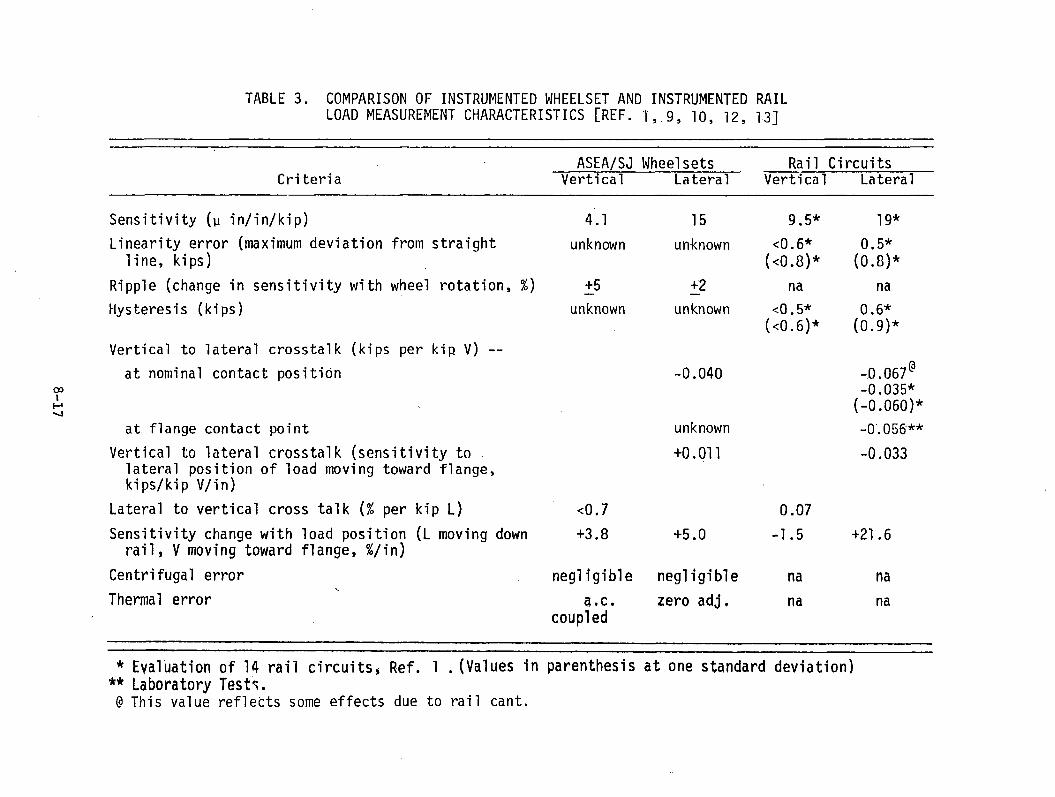
8-17

TABLE 3. COMPARISON OF INSTRUMENTED WHEELSET AND INSTRUMENTED RAIL LOAD MEASUREMENT CHARACTERISTICS [REF. 1,9, 10, 12, 13]

ASEA/SJ Wheel sets Rail CircuitsCriteria Vertical Lateral Vertical Lateral

Sensitivity (y in/in/kip) 4.1 15 9.5* 19*

Linearity error (maximum deviation from straight line, kips)

unknown unknown <0.6*(<0.8)*

0.5*(0.8)*

Ripple (change in sensitivity with wheel rotation, %) +5 +2 na na

Hysteresis (kips) unknown unknown <0.5*(<0.6)*

0.6*(0.9)*

Vertical to lateral crosstalk (kips per kip V) —

-0.067®-0.035*(-0.060)*

at nominal contact position -0.040

at flange contact point unknown -0.056**

Vertical to lateral crosstalk (sensitivity to lateral position of load moving toward flange, kips/kip V/in)

+0.011 -0.033

Lateral to vertical cross talk (% per kip L) <0.7 0.07

Sensitivity change with load position (L moving down rail, V moving toward flange, %/in)

+3.8 +5.0 -1.5 +21.6

Centrifugal error negligible negligible na na

Thermal error a.c.coupled

zero adj. na na

* Evaluation of 14 rail circuits, Ref. 1 . (Values in parenthesis at one standard deviation) ** Laboratory Tests.@ This value reflects some effects due to rail cant.

CONCLUSIONS

Loads from an instrumented wheelset can evaluate the dynamic response of a specific vehicle to a braod spectrum of track conditions over the given track route. Loads from an instrumented track site can provide an evaluation of all passing wheels (not just the instrumented wheelset) and can therefore encompass a full range of rail vehicles, speeds and operating conditions for that specific location, for comparison with the test vehicle. A judicious combination of both on-board and wayside measurements can most cost-effectively provide an evaluation of new equipment and a comparison with the existing load environment.

REFERENCES(1) Ahlbeck, D. R. , Johnson, M. R. , Harrison, H. D. , and Tuten, J. M. ,

"Measurements of Wheel/Rail Loads on Class 5 Track", Report No. FRA/ORD- 80/19, Feb. 1980.

(2) Ahlbeck, D. R., Harrison, H. D., Prause, R. H., and Johnson, M. R., "Evaluation of Analytical and Experimental Methodologies for the Characterization of Wheel/Rail Loads", Report No. FRA-OR&D-76-276, November 1976.

(3) Anon., Question D71, "Stresses in the Rails, the Ballast and the Formation Resulting From Traffic Loads", Interim Report No. 1, Stresses in Rails, ORE, UIC, Utrecht, Netherlands, April 1965 (D71/PPI/E(44400)).

(4) Anon., ORE Colloquia, "Measurements and Their Analysis in Railway Technology", Report No. 1, 5th International Colloquim of ORE/BVFA on Railway Vehicle Technology, Vienna, Austrai, May 6-8, 1969 (Utrecht, October 1969, AZ 40/RPI/E).

(5) Kudryavtsev, N. N. , Melentyev, L. P., and Granovskiy, A. N. , "Measurement of Vertical Forces Acting from the Wheels of a Moving Train on the Rails", (Institute of Railroad Engineering, Moscow, USSR), Herald of the All-Union Scientific Research Institute of Railroad Transport, No. 6, 1973, pp 31-35.

(6) Question BIO, "A Comparison of the Methods of Measuring on the Track and on Wheels the Lateral Forces (Y) and Vertical Forces (Q) Caused by Rolling Stock...", Interim Report No. 11, Office of Research and Experiments of the International Union of Railways (ORE), Utrecht, Netherlands, October 1964.

(7) Tong, P., Brantman, R., Greif, R., and Mirabella, J., "Tests of the AMTRAK SDP40F Train Consist Conducted on Chessie System Track", Report No. FRA/ORD-79/19, May 1979.

(8) Question B55, "Prevention of Derailment of Goods Wagons on Distorted Tracks", Report No. 4 (B 55/RP 4/e), Utrecht, October 1970.

(9) Coltman, M. , Brantman, R. and Tong, P., "A Description of the Tests Conducted and Data Obtained During the Perturbed Track Test", Report No. FRA/ORD-80/15, January 1980.

8-18

(10) Harrison, H. D. and Tuten, J. M., "Perturbed Track Tests Wayside Measurements", Interim Report to DOT/TSC by Battelle, Columbus Laboratories, Contract No. DOT/TSC-1595, August 1979.

(11) Modransky, J., Donnelly, W. J. Novak, S. P. and Smith, K. R., "Instrumented Locomotive Wheels for Continuous Measurements of Vertical and Lateral Loads", ASME Paper 79-RT-8.

(12) Andersson, E. , Anderson, T. J., and Nilstam, N. G., "Computation and Measurement of Track Forces and Running Properties. A Comparison Between Theory and Experiment", ASEA Report TKM 1978-11-22/EA.

(13) Thompson, W. I., III, "Plate Instrumented Wheelsets for the Measurement of Wheel/Rail Forces", Report No. FRA/ORD-80/58, Oct. 1980.

(14) Kesler, K. , Yang, T-L., Mahone, G., and Boyd, P., "The Design and Application of Instrumented Wheelsets for Measuring Wheel/Rail Loads", ENSCO, Inc., presented at ASME Winter Annual Meeting, New York City, December 7, 1979.

(15) Ahlbeck, D. R., "An Investigation of Impact Loads Due to Wheel Flats and Rail Joints", ASME Paper No. 80-WA/RT-l, November 1980.

8-19/8-20

WAYSIDE MONITORING OF WHEEL/RAIL LOADS Steven R. Benton PORTEC, Inc.

Railway Products Division Oak Brook, 111. 60521Introduction

It has become important to research and test organizations in the railroad industry in recent years to have the capability to measure and monitor wheel/rail loads that are produced in track. Not only the capability to measure but also to monitor and record these readings. One of the prime reasons for these measurements is to determine exactly what environment the track system experiences. Wheel/rail loads are a major input into this environment. Another factor is lateral to vertical (L/V) loads for a section of track since they are an important design consideration in constructing a track system and in operating traffic over that system. The design of equipment used by the railroad industry has to withstand the load environment the wheel/rail interface produces and it is, therefore, important to railroad equipment manufactures to know these inputs. Therefore, a great deal of research work has been done on developing measuring techniques for determining the wheel/rail load.

There have been a number of technical papers published, foreign and domestic, on taking of track measurements. An area that has had much less work done and is of equal importance, is in techniques of monitoring and processing wheel/rail load data once it has been measured. A number of different methodology's exist as to monitoring but little exists as to how to apply these methods to individual measurement requirements. It is the intent of this paper to discuss one of these methods and how it applies to the monitoring and processing of wheel/rail load data. The techniques employed and experience gained in designing and constructing a monitoring and recording system for wheel/rail loads will also be considered.Background

The characterization of the wheel/rail load environment has been a requirement for many years. This data has been important for the safe and reliable design of track components such as joint bars, tie plates and tie fastening systems and for the design of car and locomotive components such as wheels, bearings, and suspension systems. This type of data also has an important role in the testing laboratory. With the development of more sophisticated mechanical and electronic testing equipment it is possible to simulate portions of the track environment in the test lab. In order to produce the correct wheel/rail load environment it is necessary to know

9-1

exactly what these loads are. It is possible to use the data measured from track as a direct input into this test equipment thusly simulating the environment encountered in the track.

Various sources have been used to obtain data on wheel/rail loads.Much of this data comes from commercial and governmental testing groups.The railroad industry has also conducted some testing, usually for their own requirements and usually unpublished. Since the sources of data that exist are limited and because much of the data would not satisfy existing requirements, it became evident that additional data would be needed and a system to make these measurements would be necessary. This system would be used to monitor and record wheel/rail loads and other track related data in an in-service environment. The fact that this system would be used for in-service field testing brought forth the question of what form the overall system should take? Should the system be portable or mobile abroad some type of vehicle? Should the system be a manned system or be an unmanned, data logger type system? There were also questions as to what types of instrumentation to use. Would this be an analog or digital system? The measurement technique that would be used to measure wheel/rail load was also a question. Since the track loading data that was needed would be used for a number of different requirements, the type of measurement technique that was used would be important. The techniques considered at the time were; the instrumented tie plate to measure vertical rail load; the instrumented rail technique using strain gages applied to the rail to measure vertical and lateral loads; and the use of a vehicle born system using an instrumented wheel set to monitor vertical and lateral loads. Since some of the testing would be done on concrete tie track and would prohibit the use of instrumented tie plates and the cost considerations and operation of an instrumented wheel set were prohibitive, it was decided to use the instrumented rail technique using strain gages applied to the rail to measure vertical and lateral load.

Testing requirements at the time were to monitor and record data from track under different operating conditions. This would include both concrete and wood tie track. In order to move from location to location the system would need to be portable. The amount of track instrumentation being considered and the operating environment precluded using the unmanned

9-2

data logger approach. It was, therefore, decided for ease of operation and portability to construct a system mounted in a vehicle. This vehicle would allow the system to be transported to any site where measurements were required with a minimum of effort.

The instrumentation to be used to monitor the track data was of prime consideration. The system had to have the capability to monitor numerous data channels at the same time and also record them. There would also need to be provisions to look at the data as it was acquired. Since there were various requirements for processing and both high and low frequency data would be looked at, it was decided to monitor and record the data in analog form and to digitize and process the results at the laboratory.Using FM analog recording equipment with general purpose solid state signal conditioning, the system would meet immediate requirements to monitor high and low frequency wheel/rail load data as well as meet future testing needs as they arose. The use of FM analog recording techniques also allowed for the recording of data for long periods of time which would be required if the wheel/rail loads from a large number of passing trains were to be monitored.System Construction

The data monitoring and recording equipment was mounted in a small 3/4 ton cargo van. This van was used because of its availability at the time and because it would be maneuverable in the areas where testing would be conducted. Some of these areas would prohibit access by a large van or motor home. Use of 48 inch equipment racks shock mounted in the van allowed the equipment to be easily accessible for operation and maintenance. The FM analog recorder that was used could record 14 channels of data directly onto tape. Since 14 channels would meet our immediate requirements it was decided to limit the overall system capability to 14 channels. Two racks of 8 solid state signal conditioner/amplifiers were installed in the van of which 14 were wired into the FM analog recorder leaving 2 of the signal conditioner/amplifiers for use as spares. A 14 channel light beam oscillograph was also installed to monitor data on a "quick look" basis.The output of the FM analog recorder was wired to a patch panel which would allow access to any of the data channels during system set-up and recording. A dual channel oscilloscope, digital volt meter, and frequency counter were

9-3

also installed to be used to adjust equipment during set-up and for maintenance of the instrumentation in the field. Circuitry was also added which would allow remote calibration of track instrumentation as well as to start and stop the data monitoring equipment during data acquisition. This circuitry allowed a single button to be pushed to start or stop all the data monitoring equipment. Since most of the equipment was temperature sensitive and operations would take place in both cold and hot weather, appropriate air conditioning and heating units were installed in the van.

In most situations anticipated, test site locations would be remote and there would not be electric power available. This required that a gasoline motor-driven AC generator be provided to supply power to the monitoring equipment. To provide remote power, a 5 KW generator was installed in a utility trailer which would be towed behind the van. This trailer would also provide necessary storage space for other equipment as well as allow the generator to be operated away from the van for safety and to reduce the noise level around the monitoring van. A 100 foot power cord was provided to operate in this manner. Instrumentation to monitor voltage, frequency, and power consumption was provided in the van. Lights capable of running off both AC and DC battery power were also installed in both the van and generator trailer. This facilitated operations during night time in case of power failure.

In order to operate a safe distance from the track at a test location, a single, multi conductor, instrumentation cable was used to connect the track instrumentation to the monitoring van. With the track instrumentation and monitoring equipment used, this cable could be approximately 200 feet long without having to use preamplifiers at the track and without an excessive amount of noise induced on the data lines. In order to connect the track instrumentation to this cable, a track side junction box was constructed with 14 environmental connectors for inputs from track instrumentation and one environmental connector for output to the monitoring van. The remote junction box also provided a location to install calibration circuitry to calibrate the track instrumentation. Connection of track instrumentation to the junction box was done using various custom made instrumentation cables. By using the track side junction box these cables could be made much shorter than if they had to run to the monitoring van.

9-4

Custom cables also reduced the number of environmental connectors that would need to be used.System Operation

Once a test site location was established and access had been gained to this location by the monitoring van, the instrumentation of the test site would be started. The application of strain gages to the rail to measure vertical and lateral wheel rail loads was done first, using weldable strain gages. Although weldable gages are rather expensive, they are easily installed with little surface preparation and are usually supplied environmentally protected, each having its own pigtail leads. The leads from each vertical and lateral strain gage circuit were gathered together and each circuit was connected to a cable running to the junction box.Solder connections were made to these leads and the connections were environmentally protected using heat shrinkable tubing and silicon rubber (RTV). This established a good electrical and water-proof connection. Once all the vertical and lateral wheel/rail load circuits were connected to the junction box, connection was established to the monitoring van through the 200 foot instrumentation cable. The system integrity of each circuit was then checked out from end-to-end. The noise level on each channel was checked and if excessive, adjustments made.

Calibration of each of the vertical and laterial strain gage circuits was accomplished by using a calibration rig consisting of a hydraulic jack, calibrated load cell, and jacking frame. This rig allowed accurate known loads to be applied laterally, vertically, or in combination to each strain gage circuit. The calibration curve for each lateral and vertical strain gage circuit could be established and appropriate shunt calibration resistors found. These calibration resistors were then installed in the monitoring equipment circuitry to allow shunt calibrations to be made on each data run. As previously mentioned, internal circuitry allowed a shunt calibration to be made and recorded on each data channel at the start and end of each data run. This information was then used to establish scaling factors during data reduction.

After the track instrumentation had been calibrated, the system was ready to record data from passing traffic. When a train approached the instrumented test section a data run would be initiated by pressing

9-5

the "start" button. This would start the FM analog recorder and light beam oscillograph as well as initiate a shunt calibration of each of the data channels simultaneously. After the train passed the instrumentated test section the "stop" button would be pressed which would initiate another shunt calibration and then stop the recorder and oscillograph. After each run the data recorded on tape was played back through the light beam oscillograph to verify that it had been recorded. The monitoring equipment was then reset to record the next passing train. This operation was repeated until a sufficient number of wheel/rail loads had been recorded. In order to record 40 to 50 passing trains it would require that a test site be monitored for 2 to 3 days depending on traffic.Data Reduction

Data reduction arid analysis requirements were established before field testing was started in order that the data recorded would meet the final analytical requirements. The initial data analysis requirements were to measure and print out all the peak vertical and lateral wheel loads and to plot histograms of these loads for each passing train. Another-requirement was to calculate vertical to lateral (L/V) loads for each passing wheel.Since each wheel load created an output to the system, a comparison of wheel data could be made to individual cars using consist lists obtained from the railroad. High frequency analysis of the vertical and lateral wheel/rail load could also be made. In order to accomplish these requirements, the data was digitized in the laboratory by replaying the analog data into the laboratory computer a number of times using various scan rates. This technique would not be possible if the data was digitized before it was recorded in the field. The digitized wheel/rail load data could also be used as a controlling input to the laboratory servo-hydraulic testing equipment, allowing laboratory test specimens to be subjected to the loads as they exist in track.Conclusions

Techniques for measuring wheel/rail loads are'still being refined and new methods are still under investigation which will allow wheel/rail loads to be measured easily and with greater accuracy. Along with the development of more accurate measuring techniques will be more sophisticated monitoring equipment. Microprocessor and minicomputer based systems are already on

9-6

the market which allow a large number of data channels (30 to 40) to be acquired, digitized and recorded at rates fast enough to analyze the high frequency content of the data. The type of monitoring system used for each test will have to be determined from the data analysis requirements. It is important that the techniques used to acquire the data are compatible with the methods used to monitor and record data. Each requirement of the test needs to be considered and well planned ahead of schedule in order that the final data obtained is correct.

9-7

DISCUSSION

Mr. Ahlbeck: Don Ahlbeck, Battelle. Did you apply any of the one-inch gages to the high rail of sharp curves and, if so, did you have any failure problems with it?

Mr. Benton (PORTEC): We apply gages to both low and high rail, and Ithink the largest curve that we've tested to date is about 6 degrees. We have never had an ELTEC gage fail in the field, but we haven't really done that many measurements to say they're not going to. But we haven't seen any failures yet. I know this has been a problem with these gages that has been seen.

Mr. Caldwell: Caldwell from CN Rail. I'd like to put a question to you,Mr. Benton, and also for Harold Harrison. In connection with the lateral force measuring circuits that are used, the circuit is essentially monitoring or responding to shear strain on the base of the rail which can arise from lateral fluctural shear when the wheel is between two measuring stations, and also from torsional shear which may occur when the wheel is removed or outside the measuring station. I note that the calibration procedures tend to apply the load, the question is really how do you calibrate them? The ones I see you talking about apply the load outside the measuring station, would the gages still respond and therefore, how do you avoid the crosstalk from other wheels down the track?

Mr. Harrison (BATTELLE): I guess I can give you the answer to thatbecause our laboratory has studied that problem. We did determine that basically the wavelength of shear load taken at the rail outside the zone is typically long enough that the difference is quite small and therefore cancels out to a very low number. More importantly, there is actually the degradation in the crosstalk sensitivity to vertical load as you approach the edges of the sensitive zone and that sort of thing. However, fortunately, it is added to the center and so what we do then is simply restrict our data sampling procedure. We only sample when it is centered and at that point the input from outside forces is negligible.

Mr. Tong (TSC): I think of of the worst problems of field testing isreally how to apply the gages. Maybe you can tell us from experience how you actually put a gage in, how difficult it is, and what kinds of things one should watch out for. That's Question 1. Question No. 2, I think Don alluded to, it that we do have some problem of failure of the gages in high curves. Maybe he can tell us how this gage failed and how we cope with this problem.

Mr. Benton: If I might quickly answer your first part, the weldablegages worked out very well. All that's needed is just grinding of the rail to get a surface to put the gage down on. Of course, the environmental problems with trying to put a bondable gage on in the field can be disastrous. But the techniques involved with weldable gages are easily gained by experience, and it allows for the capability to measure these loads in the field rather quickly and, besides the initial cost of the gages, fairly inexpensively.

9-8

Mr. Ahlbeck: I might add that both the key fellows from HITEC are hereat the conference, Steve Wnuk and Doug Unkel, and if anyone is interested they would probably be very glad to give a pitch on installation of their gages. We worked-with both the ELTEC and the HITEC gages, and the installation procedures are nearly identical. They both add a stainless steel shim. We've found that people who have used weldable gages in other applications of severe environments have not had the same problems necessarily that we've had in rail applications. Primarily, there seems to be some differences in the rail steel properties. Other than that, if anybody has any further questions we can discuss it later.

9-9/9-10

RAIL LOAD MEASUREMENTS ON A SUBWAY SYSTEMJ. R. Billing

Ontario Ministry of Transportation and Communi cat ions 1201 Wilson Avenue

Downsview, Ontario, Canada M3M 1J8The Toronto subway has cars of three age groups. The cars of the two older groups have a tendency to hunt at cruising speeds, while the newer cars are stable. Rail wear patterns have developed on tangent track with a wavelength corresponding to the frequency and velocity of the hunting cars. An investigation has been launched into the lateral dynamics of the cars, rail loads, and the economics of car and track, refurbishment, to forestall a future maintenance burden. This paper describes the rail load measurements.Two test sites were selected, one with new rails and one with a well developed rail wear pattern. Strain gauge arrays to measure vertical and lateral rail loads were installed at ten locations over a distance of 11 m (38 feet) at both test sites. A procedure was developed whereby the strain gauge arrays were completely built up and tested in the laboratory prior to installation. This greatly reduced the time required for installation, and provided excellent quality assurance and consistency of calibration.Data was recorded on an FM multiplex system from passes by test trains of cars from all classes of the two most recent age groups, and revenue trains. The data was digitized and processed by computer.Individual cars passing over the test sites showed load variations consistent with hunting, and also showed remarkable repeatability between consecutive passes. (L/V) ratios in the range 0.5 to 0.7 - were measured for cars of all classes at both test sites, though mean values were much less. Statistics of (L/Y) by car class and test site were developed. It appears from these that differences in wheel/rail contact conditions may lead to lower loads on worn track than new track in some cases.

10-1

INTRODUCTION

The classes of cars on the Toronto Subway may he divided into three groups by age and primary suspension. The oldest cars, classes Gl, G2, G3 and GU, are 22-28 years old and have a leaf spring supported journal box sliding in pedestals. The middle car$, classes Ml, HI, H2 and H3, are 10-19 years old, and have a coil spring supported journal box also sliding in pedestals. The newest cars, classes H , H5D and H5M, are 2-6 years old, and have a chevron rubber primary suspension. The early and middle cars have some tendency to body hunting at speeds in the range 56-72 km/h (35- 5 mph). This is more noticeable in the middle cars, as they have greater acceleration capability so spend more time in cruise between the closely spaced subway stations. The tendency to hunt of these cars becomes greater as wear increases the journal box to pedestal clearance.

The lateral dynamics of the middle cars has been examined in the past, but no scheme to alleviate hunting could be devised which did not involve major rework of the truck, so the issue was not pursued.

More recently a wave pattern of wear has become apparent on some sections of tangent track traversed by trains at cruise speed. The wear patterns have a wavelength of about 12 m (U0 feet), which corresponds closely with the wavelength of a car having a hunting frequency of 1.3 Hz while travelling at 56 km/h (35 mph). The patterns are often found adjacent to signal standards or tunnel portals, which suggests perhaps that an asymmetric pressure pulse excites the body hunting mode. It has been estimated that rail life may be reduced by perhaps one third by this wave pattern wear. However, the rela-r tively low axle loads and tangent track have not required rail replacement at the rates seen by railroads on high tonnage tight curves. Concerns were raised that gradual spreading of the wear patterns throughout the system could result in future maintenance burdens. An investigation was therefore undertaken jointly by TTC and MTC to get an understanding of the problem. Working groups of staff from both organizations were formed to investigate three principal areas:

1/ Methods to eliminate hunting of the middle age group cars;2/ Rail loads on new track and on worn track;

and 3/ Economic issues in refurbishment of cars and track.

10-2

This paper describes the -work in the second of these.

The objectives of the test were to quantify the vertical and lateral loads due to the middle age group hunting cars, and the newer cars having good stability on both new and worn track. If it is assumed lateral load, or (L/V) ratio since both groups are of approximately the same weight, is an index of wear then comparisons between loads due to car classes would permit allocation of responsibility for track wear. This then could be used with the economic analysis to reach a strategy for refurbishment of cars, track, both or neither

Two test sites were selected. The first was on an at-grade section of the Southbound track of the Yonge-University-Spadina line, just North of Yorkdale station. The track had seen only 2?g years service, and some rail wear was developing. Trackwork was 115 lb RE continuous welded rail laid on a concrete slab, using the standard TTC direct fixation fastener on nominal 0.6l m (2 ft) centres, with 1 in 20 inward cant. The second test site was in tunnel on the Westbound track of the Bloor-Danforth line midway between Donlands and Pape stations; The rail had been in service some 15 years, and was nearing the end of its useful life. Trackwork was 100 lb AR-A continuous welded rail laid on the concrete invert with the TTC fastener, also at 0.6l m (2 ft) spacing, but with a 1 in 1*0 cant. Revenue trains passed each site at speeds of 56-6U km/h (35- 0 mph).

MTC owned a dynamic data acquisition system with 2k channel capability, so it was decided to instrument one rail at each test site with ten strain gauge arrays to measure vertical load and lateral load. These arrays were placed in the centre of alternate fastener bays, so covering a distance of about 11 m (36 ft). This is about the expected wavelength of a hunting train, so it was expected that the sinusoidal trajectory of loads due to hunting would be evident, and a peak (L/V) could be estimated.

STRAIN GAUGE ARRAYS FOR RAIL LOAD MEASUREMENTStrain gauge arrays for measurement of vertical and lateral rail loads are shown in Figure 1. When centred between two fasteners, these arrays both produce an electrical output proportional to the shear force on the rail. These arrays are described in Reference 1.

10-3

Similar arrays had been used earlier on another system, but that test while eventually successful was plagued by mechanical and electrical problems. The TTC uses one rail as a signal circuit, and the other for traction current return. Interference effects from these and the car propulsion system were unknown. Installation work was only possible during three hours at night when traction power could be shut off. For these reasons effort was put into development of a procedure which would ensure a rapid, reliable and low noise installation of a strain gauge array.

The final procedure involved complete buildup and wiring in the laboratory of both strain gauge arrays for a single location. Small pieces of 0.004 inch stainless steel shim stock were cut, rubbed with No. 200 grit emery paper, cleaned and degreased. Strain gauge locations were marked, and BLH FAE12S6 strain gauges were bonded to the shim using Micro-Measurement M-bond 200 contact cement. Vertical and lateral arrays were then wired into the Wheatstone bridge circuit in the laboratory. The wire from each gauge was shielded with the shield cut back to avoid any contact with the shim or rail, and all shields for one array were joined. The finished gauge assemblies were moisture proofed with Mirco-Measurement M-Coat A and taped'to a sheet of hardboard for transport, as shown in Figure 2. Laboratory checks were made on resistance to ground of each strain gauge on its shim, on Wheatstone bridge continuity, and a real-time spectrum analyser was used to check the noise spectra. The rail profiles were measured, and a neutral axis was computed for each gauge location. The rail was rough ground to remove mill scale and rust. Just prior to gauge installation the rails were finish ground with a No. 150 grit sanding disc, cleaned and degreased, and gauge locations were marked using a template. Individual shims were then bonded to the rail using Lepage 5 Minute epoxy, and held in place using 25 mm. (l") diameter pot magnets. After about 15 minutes the magnet was removed and a piece of BLH Barrier E waterproofing compound was placed over the shim stock and short lead wires. The bridge was then connected to its lead wire inside a small plastic box which was sealed with wax. The common shield was connected to the shield of the lead which then was floated back to the data acquisition system ground bus. The leads were brought back to a metal junction box and terminated in Switchcraft C5M chassis connectors. A permanent installation like this was obtained for little extra cost or effort, and it was considered worthwhile for quality

10-4

assurance even over the short term of the test. Installation and cabling of all ten strain gauge locations was done in two three hour nights at Yorkdale, where the lead cables were under 30 m (100 ft) in length. An extra night was needed at Pape-Donlands principally for installation of the 300 m (1000 ft) lead wires.

This strain gauge procedure was tested before application. Static load tests were conducted on a short piece of rail in the laboratory to verify a satisfactory epoxy bond could be obtained, and to establish response levels.Various shielding alternatives were examined using the real-time spectrum analyser, and these were further tested in an actual application in the Greenwood yard with both cam and chopper controlled cars driving over in acceleration, coast and regenerative braking.

Strain gauge installation was very successful. Only one lateral gauge was unuseable, possibly due to an incomplete epoxy bond, and one ve. bical gauge apparently became grounded during a test. Passage of trains within an hour or so of gauge installation did not apparently affect their performance. Finally, because each strain gauge array is calibrated, the additional tolerances in this procedure over direct application of weldable gauges, as described in Reference 1, is not considered significant.

DATA CAPTURE ARP TRANSCRIPTIONData was captured using a multi-channel constant bandwidth FM multiplexing system. It provided transducer excitation, signal conditioning and calibration such that 2k data channels, consisting of 20 strain gauge bridges, two LVDT's and two load cells could be multiplexed in groups of eight onto the first three tracks of a seven track instrumentation tape recorder. Time code from a precision clock was placed on the fourth track of the recorder for synchronization on playback. A bank of eight discriminators was used to display one data track on an oscillograph recorder to monitor test progress.A block diagram of the system is shown- in Figure 3.

The strain gauge conditioning cards were set up from laboratory experience with the qualification procedure to provide a full scale in the range 53- 89 kH (12-20,000 lb). A shunt current calibration of each channel was used.

10-5

The data acquisition system vas mounted in the MTC Mobile Laboratory for the Yorkdale test, where it could be parked just off the TTC right-of-way. At Pape-Donlands the equipment was mounted in a vent shaft at the end of Pape Station, and the only problem here was the rather long time for the system to warm up the 300 m (1000 ft) lead wires.

All data channels were passed through 500 Hz anti-aliaising filters within the multiplex system.

After the test was over the FM multiplex system was returned to the laboratory. Data from each test run was played back and converted to digital form and stored on a magnetic tape for processing on the MTC IBM 3033 computer. The data capture and transcription procedure was not ideal, as it gathered data whenever a train passed rather than for the short while an axle was passing a strain gauge array. The data transcription effort in particular was rather time-consuming. However, proven equipment and procedures were used which contributed to quality assurance.

CALIBRATION OF STRAIN GAUGE ARRAYSA special assembly was designed and fabricated to calibrate the strain gauge arrays. It held hydraulic jacks and load cells, reacted the lateral jack loads between the rails, and the vertical loads between a rail and a diesel locomotive provided by the TTC. It is shown in Figure U.

The strain gauge array outputs had been found somewhat sensitive to the point of application of load, and a worn rail head was considered a difficult surface against which to react vertical and lateral loads. A small segment of a condemned wheel was therefore used to provide the contact interface, as shown in Figure 5» The contact condition could thus be assumed similar to that a train might see.

Strainsert Model FL25U-3DGKT load cells of 111.25 kN (25,000 lb) capacity were used to measure the applied loads. However, the data acquisition system was set up only for TU kN (16 ,6 6 7 lb) full scale, so loading was held just under.67 kN (15,000 lb) at Yorkdale, and under 53 kN (12,000 lb) at Pape-Donlands, to avoid saturation of load cell and lateral strain gauge arrays respectively.

10-6

Load was provided "by a compact Enerpac hydraulic jack, accumulator and pump system.

The calibration loading procedure was as follows:1/ Put a 2.2 kN (500 lb) seating load on both lateral and vertical jacks

and wait ten seconds;2/ Load up to full load, and wait ten seconds;3/ Lock the vertical jack and quick-release the lateral load, then wait

ten seconds;1*/ Release the vertical load and wait ten seconds.

An example loading is shown in Figure 6. Load was applied at the centre of each strain gauge array three times. In addition, a number of loads were done at off-centre points to investigate the effects of an off-centre load. The calibration assembly was light and easily handled, so it was found possible to apply one load about every four minutes, including moving the calibration assembly and the locomotive, and setting up.

The FM data was digitized as described above, and processed on the MTC IBM 3033 Computer. Essentially the calibration was derived from the mean ratio of the time derivatives of load release and strain gauge response as

c = mean ((dL/dt)/(dv/dt))

Repeatability for multiple loadings was found excellent for individual strain gauge arrays. Satisfactory consistency was found over all arrays, as may be seen in the summary table below:

Location Array Calibration(lb At)

Coeff. of Variation

Yorkdale Vertical 19706 0.026

Lateral 201*53 0.162

Pape-Donlands Vertical 17055 0.039Lateral 11*009 0.ll*5

Calibrations are mean values over all loadings at all locations. The small coefficient of variation for vertical load is rather satisfactory, while the larger one for lateral load perhaps reflects variations in rail clip bolt

10-7/

torque, pad stiffness and other factors.

TEST PROCEDUREData was captured following the same procedure on three consecutive days at both test sites. Recording of train passbys began during the morning rush hour, and continued into the early afternoon. After the rush hour was over and headways were extended from 2-3 minutes to 5 minutes a special four car test train, having all its cars of the same class, was inserted into thecircuit of revenue trains. This train was usually able to pass the test siteevery 15-20 minutes, and made 3 or 5 passes at 6k km/h (1+0 mph), and the same number at U0 km/h (25 mph). After these runs, the same sequence was repeated with a second test train. The cars were randomly selected by the dispatcher for the first test, and the same cars were used for the second test as far as they were available. However, since there was ten weeks between the two tests, individual cars could not be guaranteed identical for each test due to maintenance and wear. Revenue trains were recorded at both relatively heavy loadsduring rush hour, and with light loads thereafter. The duration of a traincircuit along the subway line was between 90 and 110 minutes, so usually two to four passes were recorded each day for each revenue train.

At the start of each day, and at necessary intervening points, a voltage calibration was recorded to establish zero and span of data channels. The recorders were started manually some ten seconds before a train reached the first strain gauge location, and were stopped several seconds after the last car passed. It generally took 8-10 seconds for a train to cross the entire test section. The run number and the number of the. last car of the trains were inscribed on the oscillograph record and placed on the voice track to identify the data segment. Start and stop times for digitization of each segment were also determined. Data was recorded for k2 four car test train passes and 292 six or eight car revenue trains at Yorkdale, and for 3 test trains and 277 six car revenue trains at Pape-Donlands.

Trains are assembled each day from married pairs of cars chosen apparently at random by the dispatcher, subject to a limited number of compatibility rules. There is no guarantee that one married pair will be going in the same direction or have the same neighbour pairs on two consecutive days. Trains

10-8

may be taken from service due to failure, to be replaced by another train having the same run number. In order to ensure the cars of each passing train could be identified, the train run number, car numbers and time of day were recorded by clerks on the station closest to the test site for each train during the test period.

After the test the analogue data was returned to the laboratory, where the selected portions were filtered with a low pass cutoff of 200 Hz, and digitized at a rate of 1000 samples/second onto a magnetic tape in a format compatible with the MIC IBM 3033 computer. Filtering reduced somewhat the sharpness of the vertical load response to wheel passby, but the options were limited by the equipment modules available. High impact loads due to wheel flats would not be seen due to filtering, but this was not a problem because the TTC monitors car wheels daily and trues them to remove flats to control ground- borne vibration.

The digital data was processed in two passes. The first pass consisted simply of calibration and a scan to determine mean peak vertical and lateral loads from each axle of the train passing each strain gauge location. A three millisecond (four scan) moving average was used to determine mean peak loads for a gauge location whenever the vertical load was above a trigger level of 8.9 kN (2000 lb). The average covers approximately the central 50 mm (2 inches) of the strain gauge array at 6k km/h (1*0 mph), while the duration of the signal above the trigger level was 16-20 milliseconds. Peaks were determined separately for vertical and lateral loads, since the peak lateral load often occurs slightly before or after the peak vertical load. The (L/V) ratio was computed as the mean peak lateral load divided by the mean peak vertical load, irrespective of their particular phasing, on the assumption the variation in vertical load would be small to the point where the peak lateral load occurred. The (L/V) ratio varied insignificantly for one to six millisecond moving averages, though the mean peak loads were reduced as the length of the average increased. The speed of each car through the test site was computed, and the vertical and lateral loads for each axle of a car were tagged with run number, time, date, car number and speed, and were stored on disk. This resulted in a significant compression of the data. The second pass consisted of statistical analysis of the data summarized on disk. Car weights were

10-9

estimated from the mean axle loads across all strain gauge locations, and mean value and coefficient of variation was computed for car weight, speed, and peak (L/V) ratio "by-axle-, for all car classes in test runs and revenue trains. The distribution of (L/V) ratio was also computed.

The peak loads for each strain gauge location for three passes of a particular car are shown in Figure J. Such repeatability was observed for many cars, which suggests that a car may have a specific load signature on a particular section of track. The signature may change with time due to wear and maintenance. The variation of both loads may be considered as an indication of car hunting. It was often found that the highest (L/V) occurred on the leading axle of a truck. This was true for all (L/V) ratios greater than 0.1 at Pape-Donlands, whereas highest (L/V) ratios occurred for all axles at Yorkdale. The highest (L/V) ratios, up to 0.7l, occurred for the older and middle cars at Yorkdale, while the new cars there gave no more than 0.5. At Pape-Donlands, where none of the oldest cars operate, (L/V) ratios up to 0.5 - 0.6 occurred for cars of both middle and newer groups. The magnitude of these (L/V) ratios on tangent track are perhaps somewhat surprising, though the mean values are much less. A typical summary of mean maximum (L/V) ratio for the lead axle is presented below:

CarClass

Test RevenueYorkdale Pape Yorkdale Pape

Ml 0.303 0.219 - 0.212HI 0.251 0.183 0.227 -

H2 0.231 0.295 0.3U9 0.209H3 - - - 0 .1 72

Hi 0.211 0.332 - 0.205H5D 0.223 0.19 8 0.215 0.211*H5M 0.222 0.159 - 0.186

Absence of an entry in the revenue column indicates that class of car does not run on that line. Only a small number of H2's run through Yorkdale.

Several deductions can be drawn from this table. The Ml, HI, H5D and H5M test cars appear reasonably representative of the overall car population, whereas the H2 test cars may not be, and the Hi test cars apparently exhibit "rogue"

10-10

behaviour at Pape-Donlands. At Yorkdale on nev track all the never cars have lover mean (L/V) ratios than all middle cars,and also lover coefficients of variation. This might be expected from the difference in hunting tendency. Hovever four of the six classes have lover (L/V) ratios on the vorn track at Pape-Donlands. The frequency distributions for H5D cars are presented in Figure 8, shoving that the cars at Pape-Donlands also have somevhat less variation than those at Yorkdale. It is evident that vheel-rail contact conditions may differ substantially betveen the nev and vorn rails at the tvo test sites. Earlier analysis indicates that the lateral stability of the middle cars is increased somevhat vith an increase in effective conicity, vhereas for the nev cars it is reduced.

DISCUSSIONThe strain gauge array installation procedure vas very successful, as the calibration results indicate. The procedure vas mainly devised to maximize productivity during the three hours at night vhen traction pover could be removed. Hovever, the benefits to quality assurance from strain gauge array buildup in the laboratory quickly became evident and this procedure is recommended vhenever schedule constraints and cold veather do not oblige in- situ array buildup using veldable strain gauges.

Data capture used equipment immediately available vithin MTC and vas not ideally suited to the task. The data transcription step vas rather time- consuming and costly, and vould be circumvented by an on-site mini-computer data acquisition system. Data processing vas straightforvard due to the stability of the instrumentation and highly repetitive nature of train passes.

Data vas captured from a large number of cars, both in test trains and revenue service. Loads due to a specific car appear to exhibit patterns consistent vith their hunting characteristics, and shov good repeatability for different passes. This suggests an instrumented track might be a useful method to evaluate the track load potential of various cars or suspension options. Individual (L/V) ratios in the range 0.5 - 0.7 vere observed for cars of all ages, vhich might be considered high for tangent track. Statistics vere computed for h-1 T car classes, and the mass of data available provides opportunity to gain much insight into relationships of track loading by the

10-11

various car classes. At this point, with the analysis still underway, it is clear that observations from this data will be a useful contribution to the problem investigation, and could also have broader application.

ACKNOWLEDGEMENTSThe facilities and resources of the Toronto Transit Commission subway were made available by Messrs. I. G. Hendry and M. G. Brookfield, and instrumentation and data acquisition was provided by Messrs. W. R. Stephenson, J. W. Wagner and L. Pena of MTC Research Laboratory. The invaluable efforts of these and their staffs is gratefully acknowledged.

REFERENCE1. Ahlbeck D. R. and Harrison H. D., "Techniques for Measuring Wheel/Rail

Forces with Trackside Instrumentation”, Paper 77-WA/RT-9, ASME Winter Annual Meeting, 1977*

10-12

LATERAL FORCE MEASUREMENT

FIGURE 1/ STRAIN GAUGE ARRAYS

10-13

FIGURE 2/ STRAIN GAUGE ARRAY ASSEMBLY

INPUT FROM

FIELD MOUNTED TRANSDUCERS

FIGURE 3SCHEMATIC OF FM MULTIPLEX DATA ACQUISITION SYSTEM

10-14

16

-4 -------------1------------1------------1------------1----------- 1------------1------------1------------1------------r

TIME (SEC)

FIGURE 6/ YORKDALE CALIBRATION LOCATION 1

10-16

VE

RT

ICA

L LO

AD

(LB

) LA

TE

RA

L LO

AD

(LB

)

YORKDALE CAR 5543 (H2) SPEED 40 MPH AXLE 1

8000

7000

6000

5000

4000 i i i i i i i i1 2 3 4 5 6 7 8 9 10

STRAIN GAUGE LOCATION

^ ■ g x (■ •

, x * • V .■ g ■Iv lb A iM

i■ a ■s •

I

*

FIGURE 7 / LOADS FROM REPEATED PASS OF ONE CAR

10-18

PERCENTAGE YORKDALE PAPE

FIGURE 8 / DISTRIBUTION OF (L/V ) H5D CARS, LEAD AXLE

DISCUSSION

Mr. McConnell; Don McConnell of TSC. I won't speculate specifically on your comments about wheels and rails seeing the wear as some sort of a pattern of geometry. I will offer one piece of information, though, about four years ago, we sampled 15 sections of rail to try and develop contours for worn rails and contours for worn wheels. Out of those, 14 were sufficiently worn to constitute a fully service-worn condition. We essentially identified only 2 different wear profiles, one associated with curves and one with tangent track. Within the category (curve or tangent) the service worn profiles were consistent and appeared to be gravitating toward a single asymptotic profile which could be used for analysis purposes.

Mr. Jackson: Randy Jackson from Boeing Service International at theTest Center. The data you've presented I presume you've picked the peaks off there if we're talking about time span but maybe I didn't catch it.Did you use a wheel pulse detector?

IMr. Billing; No.Mr. Jackson: Did you use time to pick the peaks off the strain gage

readings?Mr. Billing: We picked out a data segment while the train was passing

and digitized the whole thing, and then I scanned, I set a level at about 2000 lbs. When I found all the places where the data was about 2000 lbs., then I scanned just over those regions to pick the peak values. I used the vertical to determine when a wheel was in thfe span of the given strain gage array.

Mr. Jackson; You took the maximum in the span?Mr. Billing: I took the maximum 3 millisecond moving average within

that span.Mr. Jackson: Another question. On your slides, you specified Axle 1.

Did you do a distribution for each axle?Mr. Billing: I've got the data for all axles.Mr. Jackson: Was there a heavier axle?Mr. Billing: A heavier axle?Mr. Jackson: Oilt of the four, did one fit and one bend higher as far asvertical load?

empty.Mr. Billing; No. Basically the subway cars weigh about 55 to 65,000 lbs,

1 0 -1 9

Mr. Jackson: They are uniformly distributed?

Mr. Billing: That's right. There's only a small difference due to propulsion and acceleration.

Mr. Jackson: But dynamically, they didn't distribute?Mr. Billing: Not as far as I can recall.Mr. Jackson: One last question. Are there pads underneath that track?Mr. Billing: Yes. There are, I think a half inch 60 grommet rubber.Mr. Jackson:

test sites?Did you check the condition of pads on those two different

Mr. Billing: No. We just took the track as provided by TTC. They toldus this is a section of good quality new track, this is a section of good quality worn track, and we took it as was. Some of the bolts were somewhat loose, for example, which is why I suspect there's a fairly big scatter in the lateral calibrations.

Mr. Jackson: That track is 60-inch gage?Mr. Billing:

as 5 feet.It's actually a 4 foot 10 and 7/8, but the artist drdw it

10-20

SPECTRAL ANALYSIS OF FREIGHT CAR TRUCK LATERAL RESPONSE INDYNAMICALLY SCALED MODEL EXPERIMENTS

L.M. Sweet*A. Karmel**

Princeton UniversityDepartment of Mechanical and Aerospace Engineering

Princeton, NJ 08544

ABSTRACTThe paper summarizes methods used to quantify the lateral

response of freight car trucks to random track irregularity inputs. Spectral analysis is applied to the results of an extensive series of experiments using a one-fifth scale model of a truck and half carbody, in which all inertial, friction, creep, and stiffness forces are dynamically scaled. The repeatability and confidence limits for estimates of the spectral densities of track inputs and truck response variables are determined. The influence of forward velocity, truck internal friction, and axle load on the dominant truck response modes is presented. Cross spectral methods are used to reference signals to the true track centerline, and to compute lateral response transfer functions and coherence levels. The low levels of coherence between track inputs and freight car truck/carbody response indicate that linear transfer functions do not represent the response adequately, and that measured output spectra are superior to transfer functions for comparison of truck configurations.

I. INTRODUCTIONThe characterization of freight car truck dynamics in terms of stability,

performance, and response to track inputs presents major challenges for theoretical and experimental research. The complex nature of the interactions among the truck components requires careful design, execution, and interpretation of experiments to obtain valid, meaningful results. This paper presents experimental methods useful in characterization of truck dynamics, and validates them using one-fifth scaled models.

* Associate Professor and Associate Director of Transportation Program**Graduate Research Assistant

11-1

To focus the discussion a number of issues relevant to experimental

design and interpretation of results may be raised. The conventional three-

piece truck is comprised of elements exhibiting many degrees of freedom.

Which motions or combinations of variables should be measured that best

represent truck performance? From available analytical models over 41

parameters have been suggested as being relevant to truck dynamic performance.[7]

Which parameters in a test program should be carefully controlled and varied

systematically? Nonlinear effects associated with coulomb friction, clear

ances, and wheel/rail contact are dominant factors in determining truck

behavior. This suggests that techniques used for truck excitation, re

duction of measured data, and interpretation of results be appropriate for

highly nonlinear systems. Finally, the stochastic nature of track inputs

requires a statistical representation of measured results. How many repe

titions of experiments, of what record length and bandwidth, are necessary

to obtain results that are statistically meaningful?

Methods previously used for truck lateral response characterization and

model validation have been presented in [1-3]. Experimental results pre

sented in terms of hunting velocity or time-averaged, mean-squared values of

key performance variables may be useful from a design viewpoint, but generally

are insufficient for model validation. In this paper spectral analysis of

the entire recorded time histories of response variables is used to obtain

more detailed characterization of truck lateral response over the range of

operating speeds. The use of data reduction methods, such as transfer function

analysis, that are based on the assumption of system linearity are shown to

be of very limited utility for freight car trucks.

The paper summarizes methods used to quantify the lateral response of

freight car trucks to random track irregularity inputs. Spectral analysis is

applied to the results of an extensive series of experiments using a one-

fifth scale model of a truck and half carbody, in which all inertial, friction,

creep, and stiffness forces are dynamically scaled. The repeatability and

confidence limits for estimates of the spectral densities of track inputs and

truck response variables are determined. The influence of forward velocity,

truck internal friction, and axle load on the dominant truck response modes

is presented. Cross spectral methods are used to reference signals to the

true track centerline, and to compute lateral response transfer functions

and coherence levels. The low levels of coherence between track inputs and

1 1 - 2

freight car truck/carbody response indicate that linear transfer functions

do not represent the response adequately, and that measured output spectra

are superior to transfer functions for comparison of truck configurations.

II. DESCRIPTION OF EXPERIMENTS

Vehicle Model

The experiments performed at the Princeton University Dynamic Model

Track used a one-fifth scale model of a three-piece truck supporting a half

carbody (Figure 1). The truck design modeled in the experiments is the ASF

Ride Control Truck, selected because of the availability of data character

izing its inertia, stiffness, friction, and clearance properties [4]. The

model is designed to reproduce, in scale, all dynamic forces that act on the

full scale truck in proper spatial and temporal relation. The principles of

achieving dynamic similitude in rail vehicle models are presented in [5,6].

Summarized below are the key features of the model truck design:

a) Center bolster and side frames cast of aluminum from manufacturers

drawings to achieve proper inertial scaling.

b) Wheels and rails machined to unworn profiles from a polycarbonate

resin to achieve similitude in creep forces. Wheels are backed with

steel rings to match scaled wheelset inertia.

c) Custom-wound springs to reproduce vertical, lateral, yaw, and pitch

stiffnesses and solid heights of the D-5 spring group of the proto

type truck.

d) Reproduction of clearances at the friction snubbers and bearing

adaptors. Friction surfaces at these locations are steel to

reproduce proper friction coefficients.

The model design is subject to the following similitude relations:

The truck supports a half carbody model with adjustable center of gravity

height, mass, and roll inertia, so that any carbody/lading combination may

be simulated. The carbody has lateral, vertical, and roll degrees of freedom,

with pitch and yaw restrained with a linkage system described in [6] . The

model is propelled externally (see [6]) through these linkages. In the

present model the carbody and center bolster are constrained to have the same

0.2

1.0

4.8 x 10-4 ( 1 )

11-3

roll angle, which is appropriate for small motions without rocking [7]; this

constraint may be removed in future experiments.

Instrumentation

The variables measured in the experiments are listed in Table 1. An

important feature of these experiments not previously achieved in freight

truck tests is the simultaneous measurement of track inputs and truck response.

As is shown later in the paper, such measurements are essential for cross-

spectral analysis of truck response to track inputs. Special instrumentation

includes the device shown in Figure 2 which measures lateral acceleration of

the left rail and gauge variation, plus serves as a reference for the wheel-

set displacement measurements. The yoke mounted on the front wheelset

(Figure 3) connects to two DCDT's, the latter yielding wheelset lateral

displacement and yaw angle.

The data for all signals are multiplexed and recorded on a four track

FM cassette recorder. Prior to digitization at 100 Hz the data is filtered

with a second-order lowpass filter at 25 Hz. Record lengths provide approx

imately 20 ensembles of 64 samples each. Digitized data records are stored

on tape for subsequent spectral analysis on a minicomputer.

Conduction of Experiment

Three groups of experiments are described in this paper. In the first

group tests were repeated under carefully controlled, identical conditions.

The objective of these tests was to determine the repeatability of the truck

response given identical track inputs and system parameters. The tests were

conducted at constant velocities on a 150 m scale model track section (equiva

lent to 0.75 km full scale), with rail alignments equivalent to Class 6+.

The second group of experiments explored the velocity dependence of the truck

response to the track geometry input. In the third group of tests, the

sensitivity of truck response to parametric variation in the truck was

determined. The variations selected (Table 2) emphasize the dominant role

of coulomb friction and axle load. Snubber friction is removed by retracting

the snubber wedges. Bearing adapter friction is removed by inserting a

single bearing ball in a hole drilled in the adapter crown. Axle load is

varied by applying a vertical force to the carbody.

11-4

III. DATA PROCESSING METHODS

Computation of Autospectra

The spectral analysis of each signal is based on the FFT of 20 records

of 64 samples each, using a Parzen spectral window [8], Since the spectral

estimates are computed from measured data they are subject to statistical

uncertainties. The errors associated with the spectral estimates are

determined by the data record length and the specified frequency resolution.

The 90% confidence limits are computed from [8]:

A

s <XX

/Nn Sxx (2)

Computations were performed to establish the stationarity of the measured

data. Since the confidence limits are constrained primarily by the length

of statistically uniform track, similar confidence limits are expected for

tests on full scale track.

Reference to True Track Centerline

Most mathematical models used for description of track geometry are

defined by relative variables (gauge, crosselevation) and absolute variables

(surface elevation and lateral alignment of the track centerline). While

the relative variables are readily measured, the absolute variables are

not, since neither the true track centerline nor an inertial reference are

accessible to displacement transducers. Two principal techniques used for

estimation of absolute track geometry are mid-chord offset methods and

accelerometer/relative displacement methods. To implement the mid-chord

method the offset of the rail from the midpoint of a nominally straight

reference is recorded; if the offsets of the endpoints are also known, the

three signals may then be processed using a filter that is a geometric

function of wavelength [9]. This method suffers from the fact that the

filter has infinite gain at wavelengths that are integer multiples of the

chord length, often producing spurious peaks in estimated spectra [3].

The second method employs an accelerometer to provide a signal refer

enced to inertial space, plus relative displacement transducers for conversion

of inertial data to centerline data. Processing of track geometry data in

the frequency domain is advantageous, since time integration of accelerations

is avoided. The method for data conversion is demonstrated for the apparatus

11-5

used in the present experiments. Lateral track geometry variables are shown

in Figure 4, with the associated relations summarized in Table 3. Note that

vehicle response variables referenced to the track centerline are included

in Table 3, since similar cross spectral function evaluations are required

to obtain correct spectral estimates for these variables.

For a signal composed of two random processes,

x(t) = a^x^(t) + a2X2(t) ai»a2 = CQnstants (3)

the spectral density function S for x(t) is given by [8],XX

S = a 2 S + ana0 (S S + S ) + a 2 S xx 1 1 2 v Xj X2 X2X1 2 X2X2

(4)

The cross spectral terms S in Eq. (4) are evaluated using theX • X •following identity, 1

X1X2+ S

X2X1= 2 S

X1X2cos <f>

(x lx 2)(5)

Applying Eqs. (4) and (5) to the displacement and acceleration signals in

Table 3 yields the following formulae:

Track Centerline Lateral Displacement

S66 " 4 S6-6-co ^+ 4 SA<SA<$+ 1.21 S6 ^A 6co 2 cos <J>(62A6) (6)

Wheelset Displacement Relative to Track Centerline

5 = ^ + —55-y y y y 2 1 y 6w w w w co w

1 ~.. ..

(/w 2')' co 2 2cos jj +

2 r"wu9f(7)

Carbody Roll Center Displacement Relative to Track Centerline

y Y * + —0 v cos r- + ~~A Sr xy y 2 1 y o' Y (y 60) 4 6_6_7r r co Jr 2 r 2} co 2 2 (8)

Since Eqs. (6) - (8) each include a cross spectral term, simultaneous

measurement of these variables is required (i.e. track geometry and truck

response should be incorporated into the same experiment). The above

expressions are derived for lateral displacements using the apparatus

described in this paper; similar equations may be developed for other

measurement systems for vertical and lateral track geometries.

1 1 - 6

IV. RESULTS FROM SPECTRAL DENSITY ANALYSIS Repeatability and Confidence Limits

The first group of experiments addressed the issue of repeatability in

truck lateral responses. Comparisons of the time histories of measured track

inputs showed a very high degree of repeatability as a function of position

along the track for both constant and varying forward velocities. However,

in general the time histories of the truck response variables were not

repeatable for identical test conditions, even when care was taken to

reproduce initial conditions. This nonrepeatability is the result of the

dominance of coulomb friction effects in the truck, the absence of large

perturbations in the track, and the relatively poor coherence between track

inputs and truck response (see Section V). The presence of large track

perturbations generally yields truck responses that are more repeatable in

the time domain [10].

Figure 5 shows the degree of repeatability in the estimates of spectral

densities typical for track inputs and truck response variables in the scale

model experiments. All spectra processed from measured data fall within the

90% confidence limits, demonstrating a very high degree of consistency and

repeatability in the data. This finding is very significant, since it-shows

that relatively few repetitions for each test condition are required to obtain

statistical significance (assuming that all data have been recorded success

fully] . From this information efficient test programs may be designed for

both full scale and model scale vehicles.

Dominant Dynamic Modes and Selection of Measured Variables

The spectral densities of the variables listed in Table 1 reveal two,

and possibly three, distinct modes in the lateral dynamic response. The

first mode is a wheelset kinematic hunting mode, exhibiting a strong spectral

peak in the 10 Hz to 20 Hz range with center frequency increasing proportionally

with forward velocity. This mode is exhibited by spectral densities of wheel-

set lateral displacement (Figure 6), wheelset yaw angle, carbody/bolster roll

angle, and bolster yaw angle. A carbody mode of fixed natural frequency of

about 5 Hz is exhibited by the carbody roll center lateral displacement

(Figure 7). Some spectral densities (carbody c.g. lateral displacement

and bolster lateral displacement) exhibit both modes (Figure 8). It is

also possible that a truck kinematic hunting mode exists at about 1 Hz, but

is not revealed in the spectra (1.5 Hz to 50 Hz) presented in this paper.

11-7

One of the consequences of the dominance of nonlinearities in the truck

response is the selective presence of particular modes in spectral densities

of various measured variables. In a linear system, unless a sensor is located

at a modal node, it is likely that all important low frequency modes could

be detected in the spectrum of each measured variable. Figures 6 through 8

show that this is clearly not the case for truck response spectra. It may

be misleading, therefore, to draw conclusions about truck stability and

performance solely on the basis of comparisons of measurements of one

variable. It is also possible to reconcile apparently inconsistent results

from different experiments on the same configuration if different variables

were used for analysis. It is recommended that all dominant modes of the

system be clearly identified from test results prior to inference of.relative

truck performance levels.

Velocity and Parametric Dependence of Truck Response

Figures 6 through 8 show the variation in response spectra as forward

speed is increased over the range of 10 ft/sec to 40 ft/sec model velocity.

The wheelset kinematic hunting peak increases in magnitude to a maximum at

about 15 ft/sec, then decreases in magnitude until it disappears above 20 ft/

sec. The magnitude of the carbody resonance increases with velocity over the

velocity range.

The parametric variations summarized in Table 2 have the effect of

maximizing internal friction and creep forces in Configuration 3, minimizing

these forces in Configuration 2. The baseline case for the preceding discus

sion of repeatability, modes, and velocity dependence is Configuration 1;

Configuration 4 differs from 1 only in axle load. Figures 9 and 10 display

the parametric sensitivity at the two extremes of the velocity ranges

measured. Comparisons of these spectral densities leads to the following

conclusions:

a) Internal friction and axle load are very important determinants

of truck dynamic response.

b) Bearing adaptor friction and axle load are the most important

factors in suppressing the kinematic hunting mode.

c) Friction snubbers have little effect on the kinematic modes.

d) Decreasing internal friction and axle load increases carbody

response at low frequencies.

e) Parametric differences are most pronounced at the hunting speed.

1 1 - 8

V. TRANSFER FUNCTION AND COHERENCE ANALYSIS

Method of Computation

While it is well-recognized that nonlimearities play an important role

in truck lateral dynamics, it is of great interest to determine the extent

to which linearized truck models are capable of representing the response

of the truck to track inputs. Such a determination based on experimental

evidence should be useful in guiding future development and validation of

analytical models and in interpretation of test results.

The coherence function analysis presented here assumes that the track

lateral alignment is the principal input tothe truck lateral response, so

that the truck model can be treated as a single input-multiple output

system. Alignment inputs to the two wheelsets derive from the same track

geometry plus a time delay. Cross elevation and surface profile inputs are

weakly coupled to the truck lateral dynamics, and are controlled to be

small on the Princeton Dynamic Model Track. In general, these inputs should

be measured for partial and multiple coherence function analysis [8], as

will be done in future truck response tests at Princeton.

The response of the truck to track inputs is quantified using transfer

functions derived from recorded experimental time histories. Since the

track input is broadband (see Figure 5), all system modes should be excited,

with good identification of system characteristics possible at all frequencies.

Each transfer function is derived from equations of the form,

H(f) = Sxy (f)/Sxx(f) (9)/\

where Sxy is the cross spectral density of the input variable x and the

chosen output variably y, and S is the input autospectrum. This approach

yields the optimum estimate for a transfer function according to mean

square criterion [8]. This estimate is derived solely from measured data

and is totally independent of any analytical model or assumption.

The implementation of Eq. (9) requires simultaneous measurement of

signals x(t) and y(t). A common alternative approach based on autospectra

alone is,

|H(f)| = (Syy(f)/Sxx(f))1/2 (10)

11-9

This method is appropriate for systems that are minimum phase, linear, with

negligible measurement noise [8]. The violation of the first two conditions

in the case of freight car trucks leads to very poor results, demonstrating

the inadequacy of the autospectra approach for this application.

The following cross spectral terms are required to relate response var

iables to the track centerline input <5,

Wheelset yaw angle

Bolster yaw angle

Wheelset relative lateral displacement

Carbody roll center relative S lateral displacement

(w)

These terms are related to measured variables y , y , 0_, 0 , A6, r w B w and 6

by the following equations, using methods from [8],

S l y <5 } r= I s - + I

2 bA<5y 4 1 r to 12 (S6 y + 2 ^ 6 6 to 2- r 2(11)

/\S Ay o 2 bASy 4to + ~2 (S6 y + J SA65 3to 2- w 2

(12)

sv

1 ~ 1= 2 SA60r + "2 B to

(13)

h 6w

1 ^ 1 = _ c + jL2 A<50 2W to S«2e„

(14)

Finally, the coherence squared-functions are developed in a similar manner,

being of the form,

Y.xy'

xy S S xx yy

(15)

The coherence-squared function measures the degree to which the computed

transfer function represents the associated input/output data. A high

coherence (limit of unity) indicates that most of the output can be

represented by the transfer function applied to the input. Low coherence

may be caused by presence of other inputs or dominance of nonlinearities.

1 1 - 1 0

Results of Transfer Function Analysis

Figure 11 displays coherence-squared functions for a typical output

variable for the range of velocities. Very low coherence between all output

variables and track lateral alignment inputs may be due to one or more of

the following reasons:

a) The dynamic response of the truck is dominated by limit cycle

or other nonlinear phenomena largely independent of the track

input. This occurance is consistent with the absence of large

perturbations in the model track.

b) The measured outputs are the forced response to track inputs,

but nonlinearities strongly influence the system response.

c) Unmeasured inputs (cross elevation and surface profile) that

are weakly coupled to the truck lateral response are more

important than expected.

A modest trend towards increased coherence is found at higher velocities;

it is normal for breakaway friction effects to be reduced as vibration

amplitudes increase.

Figure 12 shows a typical transfer function computed using Eqs. (9) and

(11) through (14). The 90% confidence limits are very widely spaced about

the transfer function estimate since their width increases inversely with

the coherence-squared function,

(16)

(17)

!

The low coherence in all cases makes the transfer function estimate useless

in a quantitative sense, since the wide confidence bands encompass the range

of variation found for transfer functions due to the velocity and parametric

changes discribed in Section IV. Stated another way, a transfer function

estimate from any single experiment could fall anywhere within the confidence

limits shown, and could easily be misinterpreted if used to characterize

the truck response. The estimated transfer function can be used in a quali

tative way; for example the strong hunting peak is clearly visible in Figure

12.

IH(f) I - r(f) < |H(f) | < |H(f) + r(f)

^ Swhere r^(f) + zr-^ Fn-2 *2,n-2;a ^ ^ x y ^ ^ ^

yy(f)S (f)XX v

1 1 - 1 1

As a final point it is interesting to consider the transfer function

estimate obtained using the autospectra method of Eq. (10). As shown in

Figure 12 this estimate is too large by an order of magnitude, and is even

outside the 90% confidence limits. The errors associated with neglecting

cross-spectral terms are shown to be significant in truck lateral response.

The bias in transfer function estimate is consistent with theoretical pre

dictions in [8].

VI. CONCLUSIONS

Spectral methods in the frequency domain have been shown to yield

valuable detailed information on freight car truck laterial response. Simultan

eous measurements of track inputs and truck response variables are required

for cross spectral analysis. Linear transfer functions are inadequate for

representation of truck response due to low coherence between input and out

put. The measured spectra were found to be quite repeatable and useful

indicators of the presence of dominant system dynamic modes.

Truck dynamic response has been demonstrated to be predominantly non

linear, requiring appropriate nonlinear system theory methods for successful

mathematical modeling and experiment data reduction. The important system

response modes are strongly influenced by internal friction levels within

the truck, suggesting that these parameters be carefully measured and con

trolled in truck dynamic response experiments.

The experiments described in this paper demonstrate that scale model

methods are useful in obtaining detailed data for model validation and for

development of experimental methods for full scale application.

ACKNOWLEDGEMENT

This research was sponsored by the U.S. Department of Transportation,

Office of University Research under Contract DOT-OS-60147. The freight car

truck and instrumentation were designed, built, and tested by E. Griffith,

J. Grieb, H. Dill and D. Schulte, all of Princeton University.

REFERENCES

1. Cooperrider, N.K. and Law, E.H., "A Survey of Rail Vehicle Testing for Validation of Theoretical Dynamic Analyses". ASME Trans., J. Dyn. Sys., Meas., and Control, Vol. 100, No. 4, pp. 238-251, December 1978.

2. Johnson, L., et. al., "Truck Design Optimization Project Phase II- Analytical Test Assessment Report." Wyle Laboratories, DOT Report FRA/ORD-79136, August 1979.

1 1 - 1 2

3. Fries, R.H., Cooperrider, N.K, and Law, E.H., "Railway Freight Car Field Tests", presented at 1989 ASME Winter Annual Meeting, ASME Paper No. 80-WA/DSC-7, November 1980.

4. Orr, D.G., ed., "70 Ton Truck Component Data, Physical Restraints,Mechanical Properties, Damping Characteristics," Track-Train Dynamics Harmonic Roll Series, Vol. 2, 1974.

5. Sweet, L.M., Sivak, J.A., and Putman, W.F., "Nonlinear Wheelset Forcesin Flange Contact-Part II: Measurements Using Dynamically Scaled Models". ASME Trans., J. of Dyn. Sys., Meas., and Cont., Vol. 101, No. 3,September 1979.

6. Sweet, L.M., Sivak, J.A., and Putman, W.F., "Measurements of Nonlinear Wheelset Forces in Flange Contact Using Dynamically Scaled Models."DOT Report DOT-RSPA-DPB-50/80/6, March 1980.

7. Law, E.H., Hadden, J.A., and Cooperrider, N.K., "General Models for Lateral Stability Analyses of Railway Freight Vehicles," DOT Report FRA-0R§D-77-30 (NTIS PB 272372), June 1977.

8. Bendat, J. and Piersol, A., Random Data: Analysis and MeasurementProcedures, Wiley-Interscience, New York, 1971.

9. Krishna, M.B., Hullender, D.A., and Britley, T.M., "Analytical Models for Guideway Surface Irregularities and Terrain Smoothing". DOT Report UMTA-TX-11-0001, January 1976.

10. Tong, P., Brantman, R., Grief, R., and Mirabella, J., "Tests of the Amtrak SDP-40F Train Consist Conducted on the Chessie System Track."DOT Report FRA-OR^D-79/19, May 1979.

NOMENCLATURE

Be

F

H(f) , H(f)

n

spectral resolution bandwidth, Hz (= 1/T )

F-st!atistical distribution (=F(n,a))

true and estimated transfer function

number of statistical degrees of freedom (= 2 Be T)

SxxSxy

S , S xx xyT

Tr

/\

yr’

A

true autospectrum of x

true cross spectrum of x and y

spectra estimated from measured data

total data length, sec.

record length, sec.

carbody roll center displacement rel. to track centerline

wheelset displacement rel. to track centerline

measured displacements rel. to left rail (see Table 2)

11-13

2 " 2 Y Y 1xy ’ 'xy

a , ( 1 - a )

true and/estimated coherence-squared functions for variables

x and y

absolute lateral displacements of right and left rails.

absolute lateral displacement of track centerline

track gauge variation?Chi-squared distribution (= X (n,a))

statistical confidence limits (e.g. (0.10, 0.90))

TABLE 1

VARIABLES MEASURED IN SCALE MODEL EXPERIMENTS

Variable

Left rail lateral acceleration

Rail gauge

Front wheelset lateral displacement relative to left rail

Front wheelset yaw angle

Bolster lateral displacement relative to left rail

Bolster yaw angle

Carbody lateral acceleration

Carbody roll angle

Forward velocity

Axle load

Symbol Transducer

*2 Accelerometer

AS Leaf spring w/ strain gage

^w DCDT

0w DCDT pair

A

yB DCDT

9B Geared potentiometer

hAccelerometer

*B Geared potentiometer

V Drag wheel w/tach

AF Load cellz

11-14

TABLE 2

CONVERSION BETWEEN MEASURED AND TRACK CENTERLINE VARIABLES

Variable Symbol Definition

Track centerline lateral displacement 6 1 ( V « 2) " S:

Track guage variation AS V « 2Front wheelset lateral displacement

relative to track centerline

A

y + Sn

Carbody roll center lateral displacement

relative to track centerlineyr yT * «2

TABLE 3

PARAMETER VARIATIONS USED IN SCALE MODEL TESTS

Configuration Friction Snubbers Bearing Adaptor Friction

Model , Loads,

1 ON OFF 25

2 OFF OFF 25

3 ON ON 25

4 ON OFF 40

11-15

11-16

Figure 1 - Dynamically scaled model of three-piece freight car truck with half carbody.

Figure 2 - Track geometry measurement device used to sense rail lateral acceleration and track gauge variation.

Figure 3 - Yoke mounted on front wheelset to measure lateral displacement and yaw angle.

11-17

IN E R T IA L REFERENCE

Figure 4 - Definition of lateral track geometry variables.

RRIL ALIGNMENT (MM)

(SAMPLED RT 100.0 HERTZI

Figure 5 - Demonstration of repeatability of track input and truck response spectral densities (symbols), each falling within 90% confidence limits (solid lines).

11-18

F. WHEELSET LATERAL DISPLACEMENT (MM)

Figure 5 - (continued)

F. WHEELSET LRTERRL DISPLACEMENT (MM)

Figure 6 - Velocity dependence of wheelset kinematic hunting mode as shown in spectral density functions.

11-19

ROLL CENTER LATERAL DISPLACEMENT (MM)

Figure 7 - Velocity dependence of carbody mode.

CAR LRTERRL DISPLACEMENT (MM)

Figure 8 - Velocity dependence of spectrum including wheelset kinematic hunting and carbody modes.

1 1 - 2 0

BOLSTER TRW RNGLE (DEG)

BOLSTER TRW RNGLE IDEG)

Figure 9 - Effect of truck parameter variations on wheelset kinematic hunting mode.

11-21



Figure 10 - Effect of truck parameter variations on carbody mode.

1 1 - 2 2

C O H E R E N C E

INPUT: RRIL ALIGNMENT (MM) OUTPUTS. NHEELSET TAN ANGLE (DEG)

Oo

Figure 11 - Typical coherence-squared function shows poor coherencebetween measured track input and response variable outputs.

TRANSFER-FUNCTIONINPUT: RAIL ALIGNMENT (MM)OUTPUT:F. NHEELSET TAN ANGLE (DEG)

(SAMPLED AT 100.0 HERTZ!

Figure 12 - Transfer function estimated from cross spectrum ofmeasured data (square symbols), shown with associated confidence limits (solid lines). For comparison the transfer function estimated from autospectra alone exhibits significant bias error (cross symbols).

11-23

DISCUSSION

Mr. Spencer (UMTA): Larry, in your movie where you showed the dark massvibrating and described it as a superposition of two modes , I was trying to visually decouple these modes but I couldn't do it. Could you tell me where the center of roll was with respect to the mass itself?

Mr. Sweet (PRINCETON): The center of roll was fairly low. It wasabout halfway in between the masses and the truck. And so what you're seeing there is definitely a superposition of the roll motion and the lateral motion together.

Mr. Spencer: I understand. Thank you.

Mr. Brantman: Russ Brantman from TSC. I would just caution along theconclusion that you're making regarding the transfer function capability.The coherence is very low but it may be due to the fact that you have a 6+ track system there so that the wheelsets are in no sense required to follow anything in the track or a self-excited type of motion in the force type of function.

Mr. Sweet: Yes. That was a point I was trying to make earlier, but Ithink it's very much worth emphasizing. Dr. Weinstock has also had discussions with me on this point. It's clear that if you take together these results and some of the results that have been obtained from tests in which there have been large track perturbations, we see very different kind of behavior, and this is almost behaving as an autonomous system. In the future we hope to introduce perturbations in the track so with the same model we can hopefully bridge the gap between this essentially autonomous motion and a fourth motion that you might get with a much larger irregularity in the track.

Mr. Swenson (EMD): Larry, I have a question about the scale of yourcreep forces. It's been shown that the level of friction in the field with typical contamination of the rail is much lower, than what you would get in the laboratory with a clean wheel and a clean rail, and we showed you some examples of that this morning. What are you attempting to represent in the model?

Mr. Sweet: What we're t^rying to do is to be consistent above all else.The friction levels that we have are about .3, coefficient of friction of .3, and we cleaned the wheels and rails with methyl alcohol prior to each run.It certainly is true that there's a wide range of friction coefficients that are present in the field, and I think that may be some of the conclusions which I stated about repeatability might be subject to question if you went and did these experiments out in the field where you didn't have as good control over the friction coefficient. What we're attempting to do here is to say if you controlled all the parameters to laboratory conditions, what would the system do? But this does not necessarily characterize what this particular truck would do out in the field.

11-24

Mr. Blader (TASC): The .3, does that represent .3 in the real world?Mr. Sweet; Yes. Because the coefficient of friction is dimensionless

and so that is consistent with full scale.

Mr. Blader: So you are, in effect, representing the typical tangenttrack condition?

Mr. Sweet: Yes. It's not the super-adhesion conditions that you mightfind in Dr. Kumar's laboratory.

Mr. Blader: I wonder if you could comment on the friction measure inthe field against friction measure in the laboratory in that any measure of friction requires a consideration of direction and the instrumentation.It's relatively rare that in any set of measurements somebody is really measuring a friction coefficient. Your locomotive tests, for example, you can measure the amount of track that that would effect and you get a coefficient adhesion that makes sense to use for track and in making measurements on the truck, some of the friction is being used up by one wheel of a one axle of a truck fighting another axle of the truck due to relatively small misalignments and trying to straighten it out. We've been trying to get a handle on what a reasonable coefficient of friction is, and strangely enough, looking at TDOP data that was generated for us on a particular track perturbation, we were seeing L/V ratios of .5 on non-flanging wheels. The only way that we could have, in fact, gotten the L/V ratio of .5 on a non-flanging wheel was if the friction coefficient was .5. Again, looking at pieces of data, it's hard to get a handle on it and we would appreciate somebody somewhere nailing down an authoritative field measurement of coefficient of friction that is not contaminated by other friction forces and parasitic friction forces interfering with the measurement.

Mr. Swenson: The typical friction creep curve is like the typical snowflake, and they have spent - I think it's around 15,000 hours now, some 1100 test runs just to characterize from a statistical standpoint the longitudinal friction creep relationship, and I had flashed on the screen this morning the cotaposite curve.] I think the point here is that there's no way that we can identify any coefficient of friction. It depends on, for one thing, how much creep is developed. The different ways we've gone about measuring this for lateral creep and for longitudinal creep is something that we can take up later perhaps.

Mr. Sweet: Yes. Just to set the record straight on this experiment,the way that we determined the coefficient of friction was empirically by using our single wheelset model under typical rolling conditions so it wasn't a complete sliding traction and braking type of situation. It was as close as we could come to what would be appropriate for this type of response, but it was done empirically with a separate experiment, and I think that if you were going to do a similar test in full scale, you'd probably want to do something similar.

Mr. Pocklington (BR): Much of the instrumentation that's been developedin the instrumented wheelset and the angle of attack measurements and perhaps the adaptor velocity could also be measured, would give what I would

11-25

expect, a natural ability to measure directly at any rate lateral creep characteristics dynamically. I wondered whether anybody had throught of doing it, or perhaps even thought of sponsoring somebody to do it, and what people might think about this? It could be done on regular track from the lateral force measurements coming out of the wheelset using the yaw parameter and natural velocity giving rise to a creep evaluation and hence a direct dynamic measurement of the creep characteristic including friction.

Mr. Sweet: There was a paper which was presented on that subject at the ASME meeting, and I think what's interesting is if you want to that, what Dr. Blader suggested, in a laboratory situation where you.can control the contact geometry with idealized but not realistic profile, in other words maybe a cylindrical ball on a flat plate or something of that nature, then that's okay. The problem with the approach that you've suggested is that with a real wheel/rail profile, you need to know the contact point so you know the rolling radius of the contact angle, etc., and these are things which are not directly measurable, and so to be able to measure the creepage to sufficient precision, is very, very difficult. All the emphasis has been on measuring the creep forces with instrumented wheelsets. I think we're seeing that a lot of progress has been made. It's very difficult to measure the relative creep velocity between the two contact surfaces. What I might suggest is, to go one step further than what you suggested, that really what we're interested in is what the creep forces are as the function of the body motion variables, the wheelset velocities and displacements and not with creepages. And there are a number of people who have suggested system identification techniques where you take the input-output models for the vehicle and you try and infer what the creep coefficients are using a maximum likelihood or other technique. The problem with that is you have to have a very good model of the vehicle to begin with.

11-26

FREIGHT EQUIPMENT ENVIRONMENTAL SAMPLING TESTS

Shaun Richmond William H. SneedThrall Car Manufacturing Company Association of American Railroads Chicago Heights, Illinois Chicago, Illinois

The Environmental Sampling Test is a project established by the Track Train Dynamics Program that will provide the environmental load data for the AAR Fatigue Guidelines. Using five of the basic car types (covered hopper, open-top gondola, trailer, tank, and box cars), each bolster is instrumented to measure vertical loads and side bearer loads.

In 1979 new microprocessor-based instrumentation was introduced to the AAR that provides a more efficient system of field fatigue load measurement. The paper describes the test program and this new instrumentation.

12-1

FREIGHT EQUIPMENT ENVIRONMENTAL SAMPLING TESTS CENTERFLATE AND SIDE BEARING LOADS FOR ANALYSTS

Part 1 Test Philosophy

1.0 INTRODUCTION

By far the most common cause of failure in freight car structures is by fatigue of welded joints. Accordingly, the Association of American Railroads has funded, through the Track Train Dynamics Research Program, the development of a fatigue analysis specification (Manual of Standards and Recommended Practices-Section C, Part II, Chapter VII). This specification has three main elements:

a. Methodology

The medothology used is defined in the specification. It uses a linear damage law (Miner Law) in association with a Goodman Diagram. This method of analysis was chosen because it obviates the need to establish the stress concentration in welds. When using the Goodman Diagram, it is only necessary to establish the nominal stress in welded joints.

b . Goodman Diagrams

Professor Munse of the University of Illinois has reviewed the literature and has collected a very extensive library of Goodman Diagrams for use with this specification.

c. Environmental Data

To date the least well developed element of the specification is the provision of environmental data. The methodology requires occurrence spectra for each type of car, over every type of track, and at a variety of speeds.No data on the order in which loads are applied is required since this is not taken into account in the analysis.

2.0 TEST PROGRAM

The purpose of the test program is to develop the data bank necessary to use the fatigue specification. Originally, a road test using five test cars and a data collection car was planned. In this test the fatigue data was to be recorded in the time domain by the data recording car. The time domain data was then to have been digitized and read into a computer at the AAR Technical Center. This computer would then perform the cycle counting process to reduce the time domain data to an occurrence spectrum. The test consist was to have been taken over a Variety of track classes, in a variety of weather conditions, in various parts of the country, and at a variety of speeds.

1 2 - 2

An analysis of two preliminary runs on the Rock Island Railroad and the Chessie System showed that a considerable length of track would be required to obtain statistically valid data. This would involve high testing costs and high analysis costs to reduce the data.

3.0 UNATTENDED DATA RECORDING SYSTEM

The collection of statistically significant quantities of fatigue data has been made practical by the development of unattended data recording systems. These systems take the form of miniature computers which collect time domain data from one of several gage or accelerometer channels. They digitize the data, establish the peak values of the cycles, and then count the cycles by some prescribed algorithm. In this case the "Rain Flow" counting algorithm is used.

It is important to remember that no time domain data is available from these recording systems. The system, upon interrogation, produces the occurrence spectrum directly. No other data is available. Because of the manner of presentation of results, it is not possible to combine channels at a later date. All channels must be recorded in the form in which they will be used continuously throughout the test. In this case five channels are required.

They are:

1. Total vertical force on the carbody bolster.

2. Total vertical force on the truck centerplate.

3. Total vertical force on the truck side bearing.

4. Twist moment on the carbody.

5. Car Speed

It is necessary to record centerplate force, side bearer force, and total vertical force separately because, as mentioned, it is not possible to combine these channels after the test. The total vertical force and torsional moments are used to design the carbody. The centerplate and side bearing forces are used to design the local bolster structure

4.0 RESULTS TO DATE

To date runs have been made with this system. They have been made between Chicago and Salem, Illinois, on the Missouri Pacific Railroad. For the first run the system was accompanied by the Association of American Railroads' test car. Data was taken from the system and also from the test car's existing instrumentation. For subsequent runs the system was entirely unattended. Some initial problems were encountered with the charging system which provides power for the unattended recorder. These problems were corrected and the system has run successfully on subsequent tests. The very limited results obtained to date have demonstrated that consistent data is being obtained. Car speed has been identified as a major parameter in determining the magnitude of vertical loads measured. This is being investigated

12-3

more carefully by arranging for one data recorder to function only at a speed in access of 50 miles per hour. Results of these tests should be available shortly.

5.0 EXTRAPOLATION TO OTHER CAR DESIGNS

The tests to date have been performed on a 70-ton box car. Clearly, the designer will require data for his own car. Initially, this data will not be available for the majority of car types. Any radically new design concept will not have data available for it at the design stage. For this reason the AAR is considering a variety of methods of extrapolating the measured data analytically. One method which is under investigation at the moment is to develop a mathematical model of the tested car and excite that model with a standard rail pertubation of various severities. A relationship could then be established between the severities of the pertubation and the size of the vertical force of the car. It would then be possible to re-state the environmental spectrum in terms of size of track pertubations. These could then be used for any car type providing a mathematical model was available for it,

6.0 GENERAL DESCRIPTION

The Environmental Sampling Test (EST) is a continuing program under Track Train Dynamics to provide environment load data for the AAR Fatigue Guidelines1 . The testing program which began two years ago used the AAR 100 research car as a data collection system. A total of five cars representing the five basic freight car types (box car, high-side gondola, tank car, piggy back, covered hopper) were to be tested as a test consist in various train routes over various railroads. The AAR 100 is manned by a crew of six.

A year ago a new data recording system was introduced that could be used in lieu of the AAR 100 for this test, reducing the manpower cost and freeing the test car for more complex test programs. Unlike the test car that records the car parameters on digital tape for cycle counting in the AAR Tech Center's Dec 20 computer, this instrumentation will count the data "on the fly" and then format and record the information for analysis. With this capability we can greatly increase the mileage which can be obtained since we now have an unmanned data acquisition system to assure that the counting procedure (Rainflow) is performed accurately, and that spurious electrical noise is effectively shielded.

The on-board instrumentation system consists of three major components that together make an integral package that can be interchanged with similar equipment. The major components consist of:

A. Instrumented Truck Bolster

B. Data Analyzer

C. Axle Power Generator

The system is currently being used on a 70-ton box car and a 100-ton ■package is in the planning stage.

12-4

7.0 INSTRUMENTED TRUCK BOLSTERThe instrumented truck bolster is strain gaged to measure 4 parameters:

1. Total vertical bolster load

2. Side bearer load

3. Centerplate load

4. Torsional load

The truck bolster was strain gaged with exploratory gages to determine the most sensitive location that produced output proportional to total bolster load regardless of load location. Once the location was determined, three bridge circuits were installed. One of these bridges was used to measure the total vertical signal, the other two circuits will be described shortly.

The second parameter measured is left and right side bearer load. The side bearer load cells also incorporate three individual bridges, one circuit of each side bearer is wired to give a plus/minus signal to correspond to left/right side bearer load. With this arrangement, one channel of the data recorded can be used to measure both signals. I will go into this when I describe the data analyzer.

The third of the parameters measured on the truck bolster incorporates the side bearer signals and the total bolster channels. The idea is to be able to determine how the load is distributed from side bearer to centerplate. This is achieved by subtracting the side bearer load cell signal from the bolster signal. With load on the centerplate, we have the total signal and as the load shifts onto the side bearers, the signal decreases to zero. This circuit uses the second of the three bridges of the side bearer load cell and the total vertical load. This is a special balanced network that subtracts the side bearer signal from the bolster signal. We call this channel the Centerplate load.

8.0 Power System

The second part of the on-board instrumentation system is the power system. Due to the power requirement of the data recording package and time interval between runs, the use of battteries alone is inconvenient. So a power package was designed to generate 12 V dc power during car movement.This power system consists of a semi-pneumatic tire against the axle. The tire is firmly held against the axle with approximately 200 lbs of force by two smaller idler wheels and adjustable spring load. The tire is connected to a gear reduction box by a double chain drive (at this point there is a 1.2:1 increase in RPM). The double chain is connected to the output shaft of the gear box which produces a 15:1 increase in RPM; thus, a total of 18:1 increase in axle RPM. Between the high-speed output of the gear box and the generator is a 30-tooth, 10 diametrical pitch gear that gives pulses to a magnetic pick up to provide speed sensing. This will be described later. Finally, the generator itself, a Leece Neville 12V, 40 amp sealed alternator that will generate power from 12 to 80 mph. The alienator output is connected to a auto-

12-5

motive-type regulator set at the factory for 14 volts. The reason for using an altenator is quite obvious since the system should generate power in both directions without polarity reversal. Because this is an altenator, it must have field current to operate, which must be provided by batteries, and this is where the magnetic pickup comes into play. This magnetic pickup produces a constant voltage variable frequency with change in RPM. Through an electronic circuit mounted near the recorder, the altenator can be switched off below a set speed of 10 mph since this is the minimum RPM at which the altenator will generate power. The output of the generator is connected to the current limiter coil of the voltage regulator and finally back to the batteries where the power is stored. The batteries wired for 12V 50 Amp hours (50Ah). These cells look much like the laboratory 1.5V dry cells we are all familiar with. Weighing about 3 lbs. apiece, these batteries will power the system for about 7 hours before sensing circuits switch the recorder system off.

9.0 DATA RECORDER

The third and most important of the system is the data recorder and peripheral devices.

The data recorder is an MTS 460 Data Analyzer. It is 11.5 in. high,18 in. wide, 12 in. deep, and weighs 30 lbs. It can take up to eight channels of bridge-type transducers and uses an eight-channel, plug-in.rainflow with mean program cartridge. This is a 40 by 40 matrix with 16,777,216 count size. The memory is a Random Access (RAM) 24K x 8K with battery back up that will keep its content for thirty days without power. Two new features are the horsepower module that is used to provide a time-at-level speed history. This is possible because the PPM frequency is converted to voltage and beat against an oscillator that cuts the voltage on and off at 100 Hz; thus, the time-at- level histogram. The other feature is RS232C software that provides control of the data recorder through the I/O port with a terminal. This provides totally remote operation of the analyzer.

The peripheral devices are a Texas Instrument 745 terminal and a STR Link II digital tape recorder. With these two pieces of equipment, a hard copy and machine readable copy of the data can be provided. The digital tape recorder can be operated by commands from the terminal.

There is another ^recorder on the market that will be utilized with the 100-ton system. It is the Electro General Datamyte 400 recorder. It is a single-channel unit consisting of a signal conditioning or high-level module,IK byte memory module, and the program module. This system, capable of counting 2 dimensional (range and mean) or 1 dimensional (range) and has a capacity of 65,280 counts and 99,000,000 counts, respectively. The system comes as a 12V or 24V operation and has numerable accessories. Operation is via an I/O port that is adaptable to many RS232 ASCII terminals.

I will now go into some detail as to operation of these two devices. Although the general operating physics is the same between.the two units, there are individual differences in describing the counting procedure. Both units use the basic pogoda-roof technique. Both units were rigorously tested using various artificial histories to assure that they do prove the same results. The data recorders start with the signal conditioning module that can

1 2 - 6

accept a quarter, half or full-bridge transducer, there is also a high-level signal module for signals such as tapered data.

Figure 1 shows the block diagram for the Datamyte 400 recorder, but it is applicable for the MTS 460 analyzer also. We see the incoming power switches and transducer to their respective inputs. At this point the transducer signal is conditioned and amplified to put the maximum signal level in the appropriate bins. The discussion of bins will be explained later on. The conditoned, amplified signal is then digitized, counted by the rainflow program, and stored in the data memory all under the control of the central processing unit. Data can then be extracted through the input/ output link to the terminal for analysis

PROGRAM D ATAm e m o r y M EM ORY

(PRo M ) (R AM )

XDCR. A / o CENTRAL e i a

C O N D I- C O N - PROCESSING SERIAL

TRANSDUCER TlO N ER VERTER UNIT INPUT/

O U TP U T

SWITCH LINK

INPUTS ^

VEHICLE ^ DC ! D C POWER SUPPLYPOWER V

terminal

Figure 2 shows the flowchart for the Rainflow algorithm, and it can be seen that a peak is first detected, it is checked to be certain it does not exceed full scale, and that it exceeds the hysteresis level. The hysteresis setting used a digital filter to accept or reject noise and parasitic signal. Figure 3 shows the results of hysteresis selection.

The peaks that occur within the hysteresis band of the last peak are excluded. The true peaks that occur outside of this band are passed on to the histogram. At the end of the test unmatched peaks are processed to form closed hysteresis loops.

12-7

PEAKS REJECTED

Hysteresis is not necessarily required in railflow counting because the smaller events are by nature of the algorithm stored in smaller bins; however, it does improve the response of the recorder and allow the program to run faster. Also the noise signals are rejected as not to fill up the bins with unnecessary data counts.

SMALL AMPLITUDE PEAKS REJECTED

HYSTERESIS REJECTION MODES

64 + TWICE FULL SCALE

Earlier in the discussion of the two systems, the work bins was used. The analog signal is passed through an A/D converter which for the MTS 460 has a sample rate of 100 KHz and 2400 Hz for the Datamyte 400. Figure 4 shows the bin configuration for the Datamyte 400, the histogram is 64 bins wide with 32 of these bins used for data storage.

USABLERANGE

FORHISTOGRAMRECORDING

4847

* FULL SCALE AMPLITUDE * 15 MEAN

3231

TENSIONDIRECTION

ZEROMEAN

COMPRESSIONDIRECTION

161 5 _______

- FULL SCALE AMPLITUDE- 15 MEAN

- TWICE FULL SCALE

DEFINITION OF FULL SCALE AND BIN CONFIGURATION

1 2 - 8

Figure 5a and b show the configuration for the MTS 460 Analyzer with 40 bins.

Element = 16,777,216

Rainflow without Mean

Rainflow with Mean

12-9

STRAINFigure 6 shows an example of a stress/ strain history and how the rainflow counting is performed. The rule for the rainflow results in a procedure that defines the cycles as closed loops. The histogram format is divided into bins of equal width from plus to minus. The number of bins that make up one cycle is equal to the strain range for that cycle. Reversal rather than cycles are actually counted where one cycle is equal to two reversals. The output is then put into cycles.

ONE-DIMENSIONAL TWO-DIMENSIONAL

Figure 7 shows the MTS version of the stress/strain response, and careful analysis produces the same philosophy in cycle counting.

Example o f ra in flow cyc le counting method

1 2 - 1 0

10.0 CONCLUSIONIn conclusion, this new type of data acquisition and analysis electronics

now provides the industry with an affordable means of collecting many miles of service data either by on-the-road analysis or from pre-recorded data without the cost of expensive test vehicles and personnel. As both companies continue development with the help of feedback provided by users like the Association of American Railroads, developments such as new, low-power microprocessors, which can drastically reduce the power consumption, may eventually result in a totally battery-powered, multi-channel system. The Association is continuing to make an effort to utilize new innovations to provide better information for the railroad industry.

The Environmental Sampling Test, by the use of the instrumented truck bolster, data analyzer with rainflow program, and unique power system, will provide some of this information.

1 2 -11/12-12

SESSION 3: DISPLACEMENT AND GEOMETRY MEASUREMENTS TECHNIQUES

THE,USE OF ANGLE-OF-ATTACK MEASUREMENTS TO ESTIMATE RAIL WEAR UNDER STEADY STATE ROLLING CONDITIONS

H. Ghonem J. KalousekCanadian Pacific Ltd. National Research Council

Montreal, Quebec Vancouver, British ColumbiaCanada Canada

ABSTRACT

This paper is concerned with the formulation of an approximate analyti

cal model describing the total wear on both high and low rails as a function

of the angle-of-attack. In this model three contact points between a wheel

set and a pair of rails on a curve are considered under steady state rolling

conditions. Based on this formula rail life is estimated and compared with

in-service field data.

DEFINITIONS OF NOTATIONS

A , A , A1 2

a

3

b

C

C123

c22

C (p), C (p)1 2

Er

F

F2

Mathematical constants

Semi-major of the elliptical area of contact

Semi-minor of the elliptical area of contact

Point of contact between right hand wheel and rail

Wheel set axis system

Lateral creep coefficient

Constants

Elastic modulus

Perpendicular force on the worn surface

Lateral creep force on the high rail

13-1

F -2Ff

f2

f -2

H

K, K , K , K1 2 3

m , m 1 2

N1

N2

P

P

qrc

S

V

V7l

wr

wr

w,

a

Y

Perpendicular force on the flange contact area

Non-dimensional creep force on the high rail

Non-dimensional creep force on the low rail

Gravitational force due to cant dificiency or unbalanced speed

Mathematical constants

Material characteristics of the rail upper surface and gauge side, respectively.

Wheel load on high rail

Wheel load on low rail

Maximum pressure on the area of contact

Constants of a polynomial function

Constants of a polynomial function

Generating radius of the wheel cone at point C

Distance slid within the area of contact

Forward velocity of the wheel set

Rigid body velocity for the right hand wheel material, i = 1, 2 and 3

Rolling velocity of the wheelset

Wear on the gauge side of the rail

Wear on the upper surface of the high rail

Wear on the upper surface of the low rail

Total wear

Cone semi-apex angle of the wheel

Longitudinal creepage

Lateral creepage

Lateral creep force on the low rail

13-2

u Coefficient of friction on the upper surface the high rail

of

Coefficient of friction on the upper surface the low rail

of

Coefficient of friction on the gauge side of theT high rail

p Poisson's ratio

V Angle-of-attack

ibYcr Critical value of angle-of-attack

Si Angular velocity of the wheel set rotation at bearings

its

n- Angular velocity component of wheel material at3 contact point C

Angular velocity component of rail material at3 contact point C

CO3

Spin creepage

I. INTRODUCTION

On major North American railways, wear, as illustrated in Figure T,

is one of the principal causes for rail replacement and is often the

deciding factor^in establishing track maintenance procedures. On C.P. Rail

a significant portion of maintenance expenditure is due to rail wear. Our

ability to improve rail life is dependent upon a basic understanding of the

rail wear phenomenon and the capability to predict the effect of wear on rail

life expectancy. This is a challenging task since the wear phenomenon is a

multidimensional process'related to a large number of interdependent para

meters.

Several attempts have been made to classify rail wear parameters into

broad categories in order to facilitate their study and thus be able to

correlate these functions in an applicable rail wear formula. The common

approach is to divide these parameters into three domains: metallurgical,

13-3

rheological and mechanical, see Refs. 1-3. The domain of interest in this

paper is the mechanical domain and is predicated on the assumption that rails

with similar metallurgy structure operating in a similar external environment

would have the same wear resistance (4-6).

Parameters comprising the mechanical domain include vehicle dynamics,

operational considerations, track structure elements and creep forces and

stresses acting in the wheel-rail interface. Under steady state rolling con

ditions, however, it is the inter-relationships between forces and creepages

that influence wear performance. Recently it was concluded by several authors

(7 and 8) that such interrelationships are governed by the magnitude of the

angle-of-attack that a wheel set forms when deviating from the radial direction

in relation to the track. Therefore, if one can succeed in correlating rail

wear in any of its forms, volumetric or rate, with angle-of-attack, which is

a measurable parameter, a quantitative wear formula could then be obtained.

The purpose of this paper is to develop such a formula.

In the next section a review of creep phenomenon is discussed and basic

assumptions are made for establishing a simplified wear formula which is

detailed in Section 3. On the basis of this formula rail life is estimated

in Section 4 while concluding remarks and a description of future research

are discussed in Section 5.

II. CREEP PHENOMENON

If a wheelset moves along the rails under the action of a purely normal

load, both wheels and rails will elastically deform in the region of contact.

While a microslip resulting from the relative local velocities may take place

between wheel tread and rail surface at points within the contact area, other

points may move together without slip. The contact area would then be divi

ded into a region or regions of slip and regions of adhesion within which the

surfaces roll without relative motion. The existence of microslip in this

free rolling pattern has been studied both theoretically and experimentally

by several workers, see Refs. 9-13. It is, however, recognized that in this

rolling condition the magnitude of microslip is very limited (14) and that

13-4

rolling resistance could be attributed to the elastic hysteresis of contact

bodies during stress cycling.

In reality the state of free rolling is prevented by the existence of

friction force at the wheel/rail interface, see Figure 2(a), by geometrical

constraints, yaw or lateral motion of the wheel set or by an application of

external force such as torque or moment-to-the-centre of a wheel. When this

occurs, tangential force will be transmitted in the contact area. As this

force is increased, the area of adhesion is progressively reduced in size

until, as the tangential force reaches its limiting value (y x the normal

force), sliding occurs over the entire area of contact. The measure of

microslip within the zone of contact is termed creepage, which consists of

longitudinal and lateral components and spin creepage. Creepage is defined

as ratio of the difference in circumfertional velocity to the mean rolling

velocity; the spin creepage is defined as the difference of angular velocity

of both wheel and rail about an axis normal to the plane of their contact

area divided by the mean rolling velocity. Within a suitable frame of re

ference both tangential and spin creepages can be determined, see Figure

2(b). As mentioned before, a relationship exists between tangential force

and creepage; the increase in the tangential force is proportional to that

of the creep component until a point is reached, at which the region of slip

occupies most of the contact area. At this state the tangential force which

reaches its limiting value, often referred to as adhesion limit, remains con

stant and does not respond to a further increase in the creepage.

The way in which creepage and spin arise in a wheel set is detailed by

many authors, see for example Refs. 15-19, and can be understood by referring

to Figure 3 in which a simple coned wheelset is shown in relation to the

track horizontal plane. The wheelset is assumed to be moving freely along

perfectly straight track with a constant velocity V in a steady state dis

placed position with a fixed yaw angle i|i. The angular velocity of the

wheelset rotation is given by ft with components (0,ft,0) in the wheelset axis

system C . Following an analysis detailed by Gilchrist and Brickie (18),12 3

rigid body velocity at point C for the right hand wheel material would be:

13-5

} ( 1 )

V- = ft r cost];1 c

V- = ft rc seca simp

V- = 03

and ft- = -ft sina3

where r is the generating radius of the cone at C and a is the cone semi

apex angle. Similarly, the material of the rail at point C in the contact

axes has velocity components (V,0,0) and ft+ = 0, where V is the forward3

velocity of the wheelset. From the definition of creepages previously dis

cussed, longitudinal, lateral and spin creepages, respectively, are written

as:

Y 1 = '(n. rc cosip - V) / Vr ,

y = (ft r seca simp) / \/ , }(2)2 c r

a) = ft sina / AT3 r

where V^, the rolling velocity of the wheelset, is:

Vr = i (V + ft r c c o s t p)

As discussed in (18),values of V and ft r , the rigid body velocity of the

wheel at point C, are reasonably similar so that the above expressions can

be reduced to:

y = cosip - 1

Y = seca sinip }(3)2

and co = sina / r 3 c

These equations are applied at the wheel tread contact point as well as

at the flange contact point for both left and right wheels. They indicate the

dependency of the longitudinal and lateral creepages on the angle ip while

spin slippage is determined by the cone angle a. This may be true for both

lateral and spin creepages; longitudinal creepage, however, can be affected

by other factors in addition to the angle-of-attack, such as the wheelset

lateral displacement (or the tracking error as referred to in Ref. 20), and

braking conditions or it can be due to tractive torque as in the case of

locomotive wheels. These factors have not been considered in the present

analysis.

13-6

For small angle-of-attack it can be shown, with reference to the previous

set of equations, that the only dominant creepage in the tread portion of a

wheel, where the cone angle a is small, is the lateral creepage which would

be equal to the angle-of-attack, ip,, under steady state of rolling. Experi

mentally, it is observed that a condition of total lateral microslip satura

tion would be reached at a value of ip equal to 20-25 minutes of arc (21)

depending on the lubricating conditions of the area of contact.

At the point of flange contact the effect of both lateral and spin

creepages will be present. Lateral creepage will be increased by the factor

seca while spin also increases as a function of ij;. Kinematically this may be

a valid conclusion; however, it is observed that for a 'hard' flanging condi

tion where, as shown in Figure 4, only small segment of the wheel asperity

orbit intersects the wheel/rail contact area, the material in this area of

contact is subjected to gross sliding in a transverse direction. The reason

for this mechanism could be attributed to the fact that the flange contact

zone is small in relation to the length of the rubbing orbit and thus the spin

component of creepage would have a small value in the contact zone. Such an

observation is substantiated by field data, results of which are described

in Figure 5 that shows nine locations of the wheel surface topography ob

tained by the use of the replica technique. The markings shown in these lo

cations are the local deformations in the area of contact caused by rail

asperities on both tangent and curved tracks over which the wheel has passed J

prior to obtaining its sufrace replica. The rubbing marks of these asperi

ties are indicative of the magnitude of the surface layer deformation and the

type of creepage the wheel surface is subjected to at each location.

The outer portion of the tread at locations 1, 2 and 3 in the previous

figure represents contact area with low rails and exhibits rubbing marks

perpendicular to the direction of motion. This can be deducted from the long

brake marks, clearly shown in locations 1 and 2, which are parallel to the

direction of travel. The direction of these rubbing marks, therefore, propose

a prevalence of the lateral creep force which agrees with the conclusion

obtained from equation 3. Locations 5, 6 and 7 represent the area of the

wheel surface contacting the gauge corner of outer rails in curves. Rubbing

13-7

marks in these locations indicate the existence of longitudinal, lateral and

spin creepages. The appearance of the latter creep component in these lo

cations may be due to the fact that the zone of these locations comes in

contact with the rail only in cases of conformal interaction. In these loca

tions the plane of contact has approximately a non-zero coinicity, thus

allowing spin moment to have an effect on the direction of the 'smearing' of

the rail or wheel material. In locations 8 and 9, however, where the 'hard'

flange condition occurs and wear of rail gauge or wheel flange material is

at its maximum, see Ref. 22, rubbing marks of asperities are dominated by

side siippage. .

Based on the above observations one may conclude the following:

1. For a wheel negotiating a curve, its contact zones at both tread and

flange, where 'hard' flanging occurs, are subjected mainly to lateral

and transverse slippage.

2. While direction and length of rubbing asperities which represent sliding

distances in the area of contact could analytically be calculated by

using for example, Kalker theory of rolling contact (23), it is accepta

ble to assume that creepage in general is a measure of the overall

amount of sliding distance in the contact zone.

Ill SIMPLIFIED RAIL WEAR FORMULA

While various types of wear mechanisms such as delamination, adhesion,

abrasion, fretting, corrosion, impact wear and surface fatigue wear are re

sponsible for rail wear, the rail life in curves is governed by the severity

of adhesive or abrasive wear. Adhesive wear on the upper surface and gauge

side of a rail occurs as a result of relative sliding between wheel and

rail. In this wear mechanism asperities of the two surfaces come into

contact and adhere strongly to each other forming asperity junction.

Subsequent separation of wheel and rail surfaces breaks these junctions

generating wear particles in the form shown in Figure 7(a).

13-8

Abrasive wear on the other hand occurs on the rail surface if hard wear

particles (white etching material), or sand grains are held between the

sliding surfaces of wheel and rail. When these particles slide on the rail

surface, they could deform the rail outer surface and subsurface by plowing.

This may result in damaging the surface layer such that a microcutting action

would take place generating wear product in a form of "chips" as shown in

Figure 7(b).

In general, these two wear mechanisms, adhesive or abrasive, can

quantitatively be described as being proportional to the load, distance slid

within the area of contact and a wear constant which is a function of the

material structure, its hardness and the degree of contamination resulting

from the interaction of the worn surface with the surrounding environment.

This type of relationship is often referred to as the Archard formula of wear,

see Refs. (24-27), and is written as:

W = m F S (4)

where W is material loss (volumetric or wear rate), m is a material constant

accounting for metallurgical and rheological parameters affecting the worn

surface, F is the applied force and S is the distance slid.

When applying the above equation to describe rail wear, three regions

on the rail head should be treated independently: the two areas of contact

on the upper surface of both high and low rails and the area of contact on

the gauge side on the high rail. On the upper surface of the high rail, the

force acting in the area of contact, as shown in Figure 4, is the normal force

N , while, as concluded in the previous section, the accumulative distance

slid in this contact area can be expressed in terms of the lateral creepage.

Wear, Wgj in this area can then be described as:

Wsi = m Ni simf; (5)

While contact conditions between the low rail surface and a wheel are

similar to those acting on the high rail, the wheel load may differ due to

the lateral displacement of the wheelset during curve negotiation. If is

13-9

the vertical wheel load on the low rail, its wear can then be written as:

l/\l = m N simp (6)S 2 1 2Total wear of upper surfaces of both high and low rail becomes

W = m (N + N ) simp S 1 1 2= simp (7)

where K is a constant equal to m (N + N )1 1 1 2

In the flange contact area, the force can be calculated by consi

dering the balance of a wheel set lateral forces as shown in Figures 4 and 7.

This results in:

Fr = (F + F _ + H) sina / (1 - y-. cosa sina) (8)T 2 2 T

where y^ is the flange coefficient of friction, F2 and F2~, respectively, are

the lateral creep force on the high and low rail and H is the force acting on

the axle due to unbalance speed or cant deficiency. In the flange contact

area the slid distance is, again, considered proportional to the lateral

creepage seca simp.Rail gauge wear, W^, can then be set as:

VL = m (F + F - + H) tana simp / (1 - y* cosa sina) (9)T 2 2 2 '

where m is a material constant accounts for the wear environment parameters2

acting on the flange/gauge contact area.

In the above equation F and F can be described by following relations:2 2

F = f y N2 2 1

and F. = f. y N2 2 2

where f2 and f2, as shown in Figure 3, are the nondimensional creep forces on

high and low rail, respectively and y is the coefficient of friction on the

upper surface of the rail. Substituting for the value of F2 and F2, equation

(9) can be written in the following form:

IaL = K (f y N + f. y N + H) simp (10)T 2 1 2 2

in which K is a constant equal to m tana / (1 - yf cosa sina)2 T

13-10

Total wear, W., on a curve is calculated as the sum of W and Wr, thus t s f ’

W = K simfj + K ( f y N + f. y N + H) s i nij> (11)t 1 2 1 2 2

Since angle-of-attack has generally a small value, s i w o u l d equal if) and

the above expression can further be simplified to:

W. = K t + K (f y N + f. y N + H ) ^ (12)t 1 2 1 2 2

In the previous expression rail wear is related to the wheelset loading

condition exerted on the high and low rails, the wheelset position in

relation to the rail direction and the nondimensional creep force in the

area of contact. As shown in Figure (8), in the region of partial slippage,

the nondimendional creep force f2 is linearly related to the angle-of-attack

until this angle reaches a critical value after which the lateral creepages

saturates the area of contact and a gross sliding condition occurs. In this

latter regime f2 is a constant value equal to the unity.

A critical angle-of-attack, ^cr, that separates the above described

two regimes can thoretically be calculated using the following expression,

see Reference (28):

^cr = 3.625 y P C (p) + C (p) log a i 2 b J

/ (a b Er) (13)

Where P is the maximum pressure on the area of contact, a and b are, re

spectively, the semi-major and semi-minor axes in the elliptical area of

contact between Iwheel and rail, E^ is an equivalent elastic modulus that is

a function of the elastic constants of rail and wheel materials, and Ci(p)

and C2(p) are constant functions of the wheel and rail Poisson's ratio p,

tabulated in Ref. 21.

For a 36 inch wheel exerting a load of 33,000 lbs. on a rail with head

contour of 12 inches diameter, Er = 30 x 106 Ib/in , p = 0.29 and y = 0.3,

values of a and b are calculated, see Ref. 29, and critical angle-of-attack,

using equation 13, is found to be:

^cr = 0.0067 rad

=23.2 minutes of arc

13-11

Experimental work carried out by Kalousek (29), showed, that gross

sliding conditions are obtained at iJj around 20 minutes of arc for dry running

conditions and at less than 20 minutes for fully or partially lubricated

conditions.

Equation (12) should then be considered for two cases; for values of

less than 20 minutes and greater than 20 minutes;

a) ip <_ 20 minutes of arc

In this case, the nondimensional creep force f2 is expressed as a function

of the creep coefficient, C22, and the angle-of-attack, \ps see Ref. (23), i.e.

f = C ip 2 22

Total wear in this regime can then be written as:

(14)

W. = K + K C ip2 (15)t 1 2 22 ' '

b) ip >_ 20 minutes of arc

In this regime, equilibrium condition (F2 = p N) exists and a lateral creep

saturation occurs in the area of contact, i.e. f2 = 1. Total wear in this

regime is then expressed as:

W. = K ij>t 3

in which K is a constant equal to K + K3 1 2

(16)

Equations 15 and 16 indicate that rail wear in curves is a nonlinear

function that increases rapidly with the increase in angle-of-attack, ip,

until a critical value of this angle is reached. At this angle, lateral

slip saturates the area of contact and wear, although greater in an absolute

sense, no longer increases exponentially but becomes a linear function of the

angle-of-attack. The significance of such equations is that wear is ex

pressed in quantitative terms since angle-of-attack can be measured by using

existing techniques under field conditions, see Refs. 30 and 31.

There are several systems that measure \p; one, which was designed by

Canadian Pacific to measure an instantaneous angle-of-attack, is detailed

in Reference 32 and briefly described in Appendix I. Experience of the

authors and others (33) in measuring angle-of-attack on curves, however,

13-12

points out that the scatter around the average value is rather large due to

curvature irregularities along any railway curve. Ideal systems for mea

suring the angle-of-attack should then be capable of providing continuous

data along the entire length of curve.

IV RAIL LIFE ESTIMATION

If the damage accumulation due to the fatigue process, which results from

the wheel/rail interaction, does not terminate the rail life prematurely, rail

life can be estimated as indirectly proportional to the wear of the rail head

as illustrated in Figure 9. Rail life, therefore, can quantitatively be

estimated by a formula similar to that of equation (14) which is a second

degree polynomial function of ip for values of ip <_ ipcr. For jp >_ , rail life

is a linear function of tJ) in a form similar to equation (15). Based on this

argument, rail life, y(^), can be described as:

y(^) = l (ip - m)2 + n ; ^ < 20<17)

y M = P if + q ; t ^ 20

where l,m,n,p and q are constants which can be, determined for a specific set

of boundary conditions. In order to test the validity of equation (16), it

was solved for boundary conditions based on data collected by C.P. Rail for

carbon rail steel. These boundary conditions are as follows:

1 - for ip = 0 (tangent track), rail life, y(^)> is estimated as 600 MGT

2 - for \p = 20 minutes of arc, which is assumed to be generated by a

majority of three-piece North American trucks in curves of 3 to

4 degrees, rail life, y(ij>), is estimated as 150 MGT. At this value

°f ^cr, dy/di can be evaluated as equal to -2.5 MGT/1 minute of

angle-of-attack.

Using this set of boundary conditions, l,m,n,p and q are calculated and rail

life is given as:

y (\p) = (ip - 21.25)2 + 148.45 ; ip < 20

y(ip) = -2.54ip + 200 ; ip > 20

13-13

Using this equation a rail life curve for C.P. main line was gene

rated and compared with the rail life of different rail metallurgies on

different railroads, as reported in Ref. 34. Results of this comparison

are illustrated in Figure 10. As shown in this figure, the theoretically

obtained curve is in agreement with and has the same characteristics as the

curves obtained from in-service field measurements. This leads to a con

clusion that the simplified approach utilized in this paper to describe rail

wear process is valid.

V. DISCUSSION

This paper presents a simplified formula for estimating rail life as a

function of angle-of-attack measurements. The correlation between the re

sults of this type of formula and field data is extremely encouraging.

Validity of such correlation should, however, be examined by further experi

mental and field tests. Presently being considered by the authors is a

series of laboratory tests using NRCC rail-wheel wear apparatus (35) to

correlate metal loss or wear rate of rail head to predetermined values of

angle-of-attack. In these tests other operating, metallurgical or

rheological parameters are to be introduced independently to observe their

effect on the sensitivity of such correlation. It is believed that if the

validity of this simplified approach is confirmed, a valuable maintenance

procedure for the prediction of rail life due to wear can be developed.

ACKNOWLEDGEMENT

The authors wish to thank Canadian Pacific Limited and the National

Research Council of Canada for permission to publish this paper.

where y (iJj) is expressed in millions of gross tons (M.G.T.) and ip in minutesof arc.

Partial funding for the track/train dynamics research investigationsin Canadian Pacific Limited has been provided by the Transportation Researchand Development Centre (Transport Canada).

13-14

REFERENCES

1. Rigney, D.A. and Glasser, W.A., Wear of Materials, ASME, N.Y. (1977).

2. Krause, H., and Scholten, J., Proceedings 5th International Wheelset

Congress, Tokyo, (1975).

3. Jamison, W.E., The 34th Annual Meeting of ASLE, St. Louis, (1979).

4. Munch, W., ISI Rail Steel Conference, London, (1972).

5. Haynes, J.M, and Babb, A.S., BSC Research Report, (1972).

6. Schumacher, W. and Heller, W., Railway Gazette International, No. 8,

(1973).

7. Kumar, S., Margasahayam, R., The General Problem of Rolling Contact,

Ed. Browne, A.L. and Tsai, N.T., ASME, AMD - Vol. 40, (1980).

8. Kalousek, J., and Ghonem, H., To be published.

9. Reynolds, 0., Philosophical Transactions of the Royal Society, London,

Vol. 166, (1876).

I10. Tabor, D., Proceedings Royal Society, A, Vol. 229, (1955).

11. Tabor, D., Symposium on Rolling Contact Phenomena, Ed. J.B. Bidwell,

Elsevier Publishing Co., N.Y., (1962).

12. Palmgren, A., Ball and Roller Bearing Engineering, S.K.F. Industries

Inc. (1945).

13. Johnson, K.L., Proc. Symp. Rolling Contact Phenomenon, Ed. Bidwell,

J.B., Elsvier Publishing Co., N.Y., (1962).

13-15

14. Eisner, E., Ph. D. Dissertatien, Cambridge University, (1954).

15. Hobbs, A.E.H., British Rail Research Report, DYN52, Derby, (1967).

16. Kalker, J.J., Vehicle System Dynamics3 Volume 8, No. 4, (1979).

17. King, B.L., British Rail Research Report, DYN37, Derby, (1966).

18. Gilchrist, A.O. and Brickie, B.V., Journal Mechanical Engineering

Science3 Vol. 18, No. 3, (1976).

19. Brickie, B.V., Ph. D. Dissertation, Loughborough University, (1973).

20. Marcotte, P., Caldwell, W.N., and List, H.A., ASME Winter Annual

Meeting, San Francisco, (1978).

21. Kalousek, J., Unpublished Data.

22. Tayler, H.A., American Society of Mechanical Engineering,

64-WA/RR-6, (1964).

23. Kalker, J.J. Ph.D., Dissertation, Delft University, (1961).

24. Archard, J.F., J. Appl. Phys.3 Vol. 24, (1953).

25. Rabinowicz, E., Friction and 'Hear of Materials3 John Wiley and Sons,

Inc., N.Y. (1965).

26. Bruwell, J.T. and Strang, C.D., J. Appl. Phys.3 (1952).

27. Rabinowicz, E. and Tabor, D., Proc. Roy. Soc. A208, (1951).

28. Engel, P.A., Machine Design, (1979).

29. Hertz, H., Proceedings Royal Society (London)3 Ser. A112, (1926).

13-16

30. Ghonem, H., Gonsalves, R. and Bartley, G., American Society of

Mechanical Engineering, Paper No. 80-RT-8, (1980).

31. Ghonem, H., Canadian Pacific Report, No. S-3480, (1980).

32. Kalousek, J. and Yee, L., Canadian Pacific Report, No. S-552-77, (1977).

33. Elkins, J.A., and Eickhoff, B.M., ASME Winter Conference, N.Y., (1979).

34. De Lucca Silva, L., and Lebre Nobrega, M., Proceedings of Heavy Haul

Railways Conferenoe3 Australia, (1978).

35. Kalousek, J., The 19th Annual Meeting for Metallurgists, Halifax, (1980).

13-17

APPENDIX 1

Instantaneous Angle-of-Attack Measurement System

Angle-of-attack or incidence \jj of a wheel running up against a rail is

the angle between its instantaneous direction of motion and the tangent in

the horizontal plane at the point of contact between the flange and the rail.

It is formed when a wheelset of a truck deviates from the radial position

while negotiating a curve.

The system to be described here is designed by Canadian Pacific to measure

an instantaneous angle-of-attack on a railway curve. It consists, as shown in

Figure 11, of three low-power lasers, three photo diode detectors and the

necessary recording system of the detectors' signals. For the system to be in

a function mode the laser beams 1 and 2, see Figure 12, should intersect each

other in the horizontal plane radially to the rail curve. This is done by a

special alignment jig equipped with an optical flat placed longitudinally on

the rail. After aligning the laser beams they should be raised about 0.25

inch vertically above the running surface of the rails. The detectors are

then to be placed in the centre of the track and laterally aligned to receive

the laser beams.

As shown in Figure 12, the angle-of-attack is evaluated as the arc

tangent of the ratio of the distance between the centers of wheel discs of

one wheelset and the distance between their flange centers. The displacement

between the centers of the two wheels is obtained by measuring the difference

between the time they interrupted and cleared the beams of laser 1 and 2.

To convert this time signal into displacement, the speed of the wheelset was

calculated from the instantaneous velocity of the wheel to travel from Laser 1

to Laser 3 which are 2.5 inch apart. Formulas presented in Figure 13 are used

to calculate the angle-of-attack from data supplied by the laser pulses as

shown in the same figure. It should be noted that these calculations depend

on the running direction of the wheelset, i.e. which of the laser beams will

be cut off first. These calculations will also be affected by misalignment

13-18

of the lasers which could provide an offset angle to be added or subtracted

from the angle-of-attack depending on the wheelset's running direction.

13-19

13-20

SURFACE FATIGUE CRACKSURFACE WEAR

PLASTIC FLOW

OF SURFACE LAYERS

TYPICAL INNER (LOW SIDE) RAIL WEAR TYPICAL OUTER (HIGH SIDE) RAIL WEAR

FIG. 1: WEAR OF RAILS IN CURVES

SLIPPED REGION

c )

BOUNDARY OF CONTACT PATCH

LOCKED REGION

B DIRECTION OF ROLLINGB ^ x

FIG . 2a: CHARACTERISTICS OF THE CONTACT ZONE BETWEEN WHEEL AND RAIL

13-21

LO NG ITUDINAL CREEP:

F IG .2b : DEFINITIONS OF CREEP COMPONENTS

13-22

FIG. 3: S IM PLE CONED WHEELSET IN D ISPLACED POSITION

13-23

IFIG. 5: SURFACE TOPOGRAPHY OF A WHEEL

SUBJECTED TO RUNS OVER TANGENT AND CURVED TRACKS

13-25

FIG . 7a: PRODUCT OF ADHESIVE WEAR, 80x

F IG . 7b: PRODUCT OF ABRASIVE WEAR, 2000x

13-27

13-28

FIG. 8: R ELATIO NSHIP BETWEEN NONDIMENSIONAL CREEP FORCE AND LA T E R A L CREEPAGE

RA

IL L

IFE

(O

F R

AIL

WE

AR

)

F IG . 9: RELATIO NSHIP BETWEEN R A IL L IF E (OR RAILW EAR), AN G LE -O F-A TTA C K AND DEGREE OF CURVATURE

700

600

500

400

300

200

100

0

iQUEBEC CARTIER RLWY (JOINTED TRACK)

N O T E S :- CONDEMNING LIM ITS - 25% HEADWEAR- R A IL SECTIONS 132 RE. UNLESS OTHERWISE SPECIFIED- R A IL CONTINUOUSLY WELDED UNLESS OTHERWISE SPECIFIED

\ y MOUNT NEWMAN CO. RLWY

• Q.N.S. & L„ RLWY - SOUTH OF ROSS BAY JC T. (CWR NORM ALLY REPLACING JO INTED R A IL)

V ITO R IA A MINAS RLWY (115 LB)

Q.NoS. & L . - CAROL LA K E RLWY

W.S. RLWY - 115 LB

HAMERSLEY RLWY | 119 LB 1 136 LB (JO INTED TRACK)

-\---1--- 1---1--- 1--- 1- + -4- + +*--- 1---5 6 7 8 9 10 11

DEGREE OF CURVATURE (°C BASED ON 100* CHORD)

THEORETICAL—i— i— * - — i— i— i

12 13 14 15 16

-t------ 1--------1---------1----------- 1------ 1--------F-4 8 12 16 20 24

H----1---- 1--- 1-----1---1----- 1--- 1-----1--- 1---- 1---1-----1--- 1-----1---'-----1---'---- 1---1---- 1---1-----128 32 36 40 44 48 52 56 60 64 68 72

A N G LE -O F-A TTA C K (MINUTES)

FIG.. 10: COMPARISON BETWEEN R A IL L IF E CURVE, TH E O R E T IC A LLY O BTAIN ED , AND THOSE DERIVED FROM F IE LD DATA

F IG . 11: A N G L E -O F -A T T A C K M EASUREM ENT SYSTEM

13-31

FIG. 12: ALIGNM ENT OF LASERS AND DETECTORS

LASER 1

LASER 2

LASER 3

J^“ 12 f^- A l2 '

i 1A j3 ^ A 13 ’

d = time interval corresponding to angle-of-attack

A12 + A12' r- — 2---- Lm secJ

T = time for 1" of travel

= ( A13 + A13‘) /2 fm seel2.5 L in J

D = - f . U n * = [rad]

= angle-of-attack

= tan~ x 60 pninj

FIG . 13: LASER SIGNAL TRACES OF A WHEELSETAND C A LC U LA TIO N OF AN G LE -O F-A TTA C K

13-32

D I S C U S S I O N

Dr. Kumar; I have some observations. I'm Sud Kumar from IIT in Chicago.I really enjoyed a rather bold and daring attempt to relate a very difficult and tough phenomenon with a very important parameter. Just for the benefit of the audience, I want to recall historically how this contribution of Dr. Ghonem has been developing in the area of angle-of-attack. Several years ago, at a meeting at FAST, we were questioning what the magnitudes of angles-of-attack will be because in our lab experiments it showed importance. Then Dr. Ghonem was invited by FAST to make measurements at FAST for the angles-of-attack and I had the pleasure of meeting him while he was making these measurements. I indeed agree very much with him that angles-of-attack have an extremely important and dominant role in the wheel/rail interaction, wear and elasticity. More recently, we have found that it even has effect on the lateral creepage magnitudes that would be developed in kinematic oscillation, the lateral displacement amplitudes that develop in kinematic oscillation mode, as well as the phase differences that develop between these parameters.

Several words of caution to this approach perhaps should be projected. As he himself has stated very clearly, metallurgical and environmental factors affect the phenomenon. In addition, we have been observing as he showed in the microscopic pictures, that the mechanism of wear that is developing in each part of the wheel is also playing a dominant role. Once we change the mechanism, the applicability of the same whole relation can also be significantly altered. Of course, these are future points of refinement and I am not in any way implying that this attempt is not a very worthwhile attempt.The longitudinal creepage has a very important role for transit wheels, for example, and its effect should indeed be added onto the angle-of-attack effect. Otherwise, the type of wheels that are there in the transit systems would not be fully accounted for.

The lateral force development that does develop in curve negotiations where the wear is significant problem is a very important influencing parameter, according to some of the tests that we have run and should indeed be incorporated, in addition to what has been done. And I'm sure that in the due course of time, some of these parameters will indeed be added on. The wear of the track and the wear of the flange is so different in character that the combination as to what instead of the whole relation should be used - it's still an unsolved problem and should still be looked at as to what exactly can be used and should be used. Archard relation is the powerful means that we have used for the determination of wear in the past, but when the mechanisms change, the modifications have got to be recognized.

One factor that plays havoc in wheel and rail wear is the types of profile coupling of the wheel and rail. If you have a cylindrical wheel, for example, or if you have a hollow profile, it has an entirely different effect on the phenomenon of wear as to how it is developing because the lateral creepage forces, the binding forces, can change very drastically.

Of course, the problem is very rough and almost too rough to tackle quantitatively at first, but this iis the way to go about slowly and keep on adding the things that should be incorporated. I really want to, first of all,

13-33

compliment Dr. Ghonem for this bold attempt, but at the same time caution that we have so many other things that must be incorporated in terms of the metallurgical, environmental profile and lateral force and longitudinal creepage effects. I enjoyed your paper very much, Dr. Ghonem.

Dr. Ghonem: I agree that there are many parameters which control thewear and, as I said at the end of this talk, the formulation given here is a very simplified approximate formulation, but it shows the way we should go.There are metallurigical parameters, there are rheological parameters. These parameters have to be delivered to these types of equations or any other types of equations very slowly, and I hope that when this sum of parameters link it to this type of formulation, we will have a quantitative formula.

13-34

MEASUREMENT, PROCESSING, AND USE OF WHEEL-RAIL

GEOMETRIC CONSTRAINT FUNCTIONS

E. Harry Law1 N. K. Cooperrider2

J. M. Tuten3

The measurement and subsequent processing of wheel and rail profile data obtained during a recent test program are described in this paper. Problems encountered during this procedure are presented and evaluated.

Using a simple wheelset model, the wheel-rail geometry parameters required as input to lateral dynamic models of rail vehicles are specified and accuracy limitations discussed. Present methods for obtaining these data are critiqued and future needs are discussed.

1 Professor, Department of Mechanical Engineering, Clemson University; Clemson, South Carolina 29631

2 Professor, Mechanical and Energy Systems Engineering, Arizona State University; Tempe, Arizona 85281

3 Research Assistant, Mechanical Engineering Department, Clemson University, (currently Research Scientist, Battelle Memorial Laboratories; Columbus, Ohio 43201)

INTRODUCTION

Railway wheelsets, as they roll along the track, are constrained to move

laterally and vertically in a prescribed manner determined by the geometry of

the wheels, rails, and track structure. The characteristics of these geometric

constraints determine, to a large extent, the nature of the lateral motions of

the wheelsets.

In this paper, a simple wheelset model is used to illustrate how the

wheel-rail geometry characteristics enter the equations of lateral motion as

system parameters and inputs. The influence on these parameters and inputs of

the "primary inputs" of (1) rail head transverse profile, (2) rail cant angle, (3) track centerline lateral alignment, and (4) gauge is then discussed.

14-1

The measurement and processing of wheel and rail profile data obtained

during recent field tests [l] is described. Further analysis of these data to

obtain estimates of the system parameters (such as effective conicity and

gravitational stiffness) and inputs (such as rolling line offsets) was con

ducted. Results of this analysis are presented and evaluated.

The objectives of this paper are (1) to indicate how wheel-rail geometry

characteristics enter the equations of lateral motion for rail vehicles,

(2) to discuss measurement and processing of wheel and rail geometry data, and present typical results, and (3) to evaluate the methods used in measurement

and processing wheel-rail geometry data.

WHEEL-RAIL GEOMETRY

For our purposes in studying the lateral dynamics of rail vehicles, we

must know the following information as a function of both the independent

variables (xw and 0 ) and the inputs due to track irregularities.

rT — instantaneous rolling radius of the left wheel

r„ — instantaneous rolling radius of the right wheel K— angle between the contact plane on the left wheel and the axle

centerline

<5r — angle between the contact plane on the right wheel and the axle centerline

<j> — roll angle of the wheelset with respect to the plane of the rails.

These constrained variables and corresponding coordinate systems are illustra

ted in Figures 1 and 2.

The dependence of these constrained variables on 0 , the yaw angle of the

wheelset, is a second order effect in most cases. Consequently, for our pur

poses it is sufficient to determine the functional relationships between the

lateral wheelset displacement (x^) and the track irregularity inputs and each

of the constrained variables.

To illustrate how these constrained variables enter the lateral equations

of motion for a rail vehicle, the lateral and yaw equations for a single wheel-

set are shown below:

14-2

l a t e r a l

F - (2f n /V) (x +r <J> -V0 )Sx 1L w oTw w

- (2f12/V)[ew-(V/ro)(SL-6R)/2]

- V W + W V " v » ( 1 )

yaw

M + (2f12/V)(x +r <i> ~V0 ) s w o w wy- (2f22/V)[0w-(V/ro)(5L-6R)/2]

- (2f33a2/V)[0w + (V/ro)(rL-rR)/(2a)]

= I 0 + I Vd. /rw2 w wi w o (2)

These equations, derived in [2], are restricted to small wheel-rail con

tact angles and embody Kalker's linear creep theory. Nevertheless, they will

serve to illustrate how the wheel-rail geometry affects the lateral dynamics.

Symbols appearing in the equations are defined in the Nomenclature. In equa

tion (1), F is the lateral force on the wheelset due to the primary suspen- sx

sion. The term involving the lateral creep coefficient, fn, is the contribu

tion to lateral creep force from the lateral creepage while that involving the

lateral-spin creep coefficient, fi2» is the contribution of the spin creep to

the lateral creep force. The terms involving N and N„, the normal forces ofL Kthe left and right rails on their respective wheels, are the lateral compon

ents of these normal forces that give rise to the gravitational stiffness.

Under suitable assumptions [2], these latter terms may be further simplified.

- v w + W V “ - V<SL-V/2 + U <3>where W. is the axle load.A

Neglecting the usually small contribution of ro<f>w to the lateral creep-

age, it may be seen that the wheel-rail geometry enters the lateral force

equation through the presence of (6 -6 )/2 in the spin creepage and in thegravitational stiffness. There is also a contribution to the gravitational

stiffness from the wheelset roll, (j>w . Note that for straight taper wheels

(such as the AAR 1/20 profile), (6 -6 )/2 will be zero while wheel-rail con-L K

tact is confined to the tread region.

In the yaw moment equation (2), M is the torque due to the longitudinaly

primary suspension. The terms involving the lateral-spin creep coefficient,

fj2, and the spin creep coefficient, f22> comprise the yaw moment due to the

14-3

pure creep moments exerted on each wheel. By far the larger term is that

due to the couple formed by the longitudinal creep forces. This is the term

involving the longitudinal creep coefficient, f33-Disregarding the small contribution of the pure creep moments, the

difference in rolling radii, (r -r )/2a, is the dominant contribution ofL i K

wheel-rail geometry to the wheelset yaw equation. On the right-hand side of

equation (2), the rate of wheelset roll, 4> > enters as a gyroscopic couplingwterm.

Each of the wheel-rail geometric constraints ((r -r )/2a, (6 -5 )/2, andL R L R

<}>w) depends on the lateral displacement of the wheelset from the actual track

centerline, x -x„. The term x is the lateral displacement from the undis- w R wturbed centerline and x is the lateral distance of the centerline from theRundisturbed centerline (also called the centerline alignment). It is given by

' XR = < V V /2where q and q are lateral distances (or lateral alignments) of the left and L Rright rails from their nominal position. x„ varies as the wheelset travels

along the track.

For the sake of illustration, consider linearizing the wheel-rail geo

metric constraints as follows:

(rL"rR)/2a = X(V V hr)/a

(W /2 = A(xw"XR“h6)/a

* v = r ( V * R - V / a ‘

(5)

(6)

(7)

The terms h , h r, and h, are offsets that account for non-zero values of ther o 9geometric constraints when the wheelset is centered, i.e. when x - x^ = 0.w RThese terms are due to1 differences in the profiles of the left and rightwheels and/or rails. A sketch of (rT-r„)/2a versus x -x„ is shown below. In

general, these offset terms could have (1) a steady non-zero value due todifferences in the wheel profiles left to right, and (2) a varying componentdue to changing differences in the left and right rail head profiles as the

wheelset travels along the track. It should be noted that the offset terms

hr, h^, and h^ enter the equations in exactly the same way as the centerline

lateral alignment, x .R

14-4

(tL-rR>/2a

w R

The linearization parameters X , A, and T can also vary along the track due to

changes in the functional forms of the geometric constraints. These changes

are due to changes in the shapes of the rail head profiles.

The gauge of the track, g, may also change along the track from the

nominal value, g .’ °o

8 * 8o + V " r (8)Gauge changes can change the functional forms of the geometric constraints and

hence contribute to changes in the linearization parameters X, A, and T. It

is possible that changes in gauge may also induce changes in hr, h^, and h^.

The sketch beloW| illustrates the effects of a gauge change from gi to g 2 on

the function (r -r )/2a for zero value of h .L K. X

14-5

We may think of changes along the track in the "primary inputs" of

(1) rail head transverse profile, (2) rail cant angle, (3) track centerline

alignment, x , and (4) gauge, g, as causing changes in the terms required to

describe mathematically the wheel-rail geometric constraints. These latter

are the parameters in the equations A, A, and T and the "mathematical inputs"

hr, hg, and h^. The influences of the "primary inputs" on the parameters and

the mathematical inputs are summarized below.

Terms Affected by Primary Inputs

a , a , rh h6* %

Primary Inputs

Rail Head Profile

Rail Cant Angle xR S

Yes

Yes

Yes

Yes

No

No

Yes

Yes

Thus, the offset terms hr, h^, and h^ can be treated as inputs to the

equations (in exactly the same way as x.,) that lump or combine the effects of

the "primary inputs", of rail head profile, cant angle, and gauge.

The parameters A (the effective conicity) and A and T (the combination

yielding the gravitational stiffness) appear as multiplying the wheelset

lateral displacement (as well as x^ and the offset terms). They are coef-Kficients in the differential equations of motion. Variations along the track

in these parameters cause what is known as parametric excitation of the rail

vehicle system. Analysis of parametric excitation for a system as complex as

a rail vehicle is a difficult task.

It may be shown [2] that crosslevel irregularities modify the lateral

acceleration of a wheelset as well as introduce a component of the gravita

tional force into the lateral force equation for the wheelset. A gyroscopic

term is introduced into the yaw moment equation for the wheelset. It is

beyond the scope of this paper to detail these effects. The interested reader

is referred to [2].

MEASUREMENT AND PROCESSING OF

WHEEL-RAIL DATA

During field tests on the Union Pacific Railroad [l], conducted in

cooperation with the Association of American Railroads (AAR), the authors

measured railhead profiles as well as wheel profiles for the test vehicle.

There were two test sites, a tangent section east on Barstow, CA, and a

curved section west of Las Vegas, both on the UP main line.

14-6

The device used to measure the rail head profiles was borrowed from the

German Federal Railways (DB) for this purpose. This is shown in Figure 3 and

is similar to the device (also borrowed from the DB) that was used to measure

the wheel profiles shown in Figure 4. The rail profilometer is easily used by

two people but can be operated by one person if necessary. Profiles for both

left and right rails could be measured at a station in less than a minute.

These profiles were reproduced on microdot encapsulated paper by a stylus

attached by a mechanical linkage to a sharp -edged follower that was traversed

manually over the rail head. Immediately after set-up of the device at a

station, it is "locked down" and vertical and horizontal reference lines are

scribed on paper newly mounted at each station. The location and orientation

of these reference lines for left and right rails are known and constant and

do not depend on the orientation of the pieces of paper on the device.

Checks for repeatability were made by mounting the profilometer at a

station, recording the profiles, disengaging the device from the rails and

then repeating the process. No discrepancies could be detected in the two

sets of profiles.

Rail head profiles were recorded at 159 stations in the various test

zones. These included two sites on the tangent test section (MP 208.5 west

for 320 feet - 65 stations; MP 206.5 east for 320 feet - 25 stations), two

curves (the 6 and 1 degree curves - about 800 feet along each - 23 and 15 stations respectively) , and the passing track (about 450 feet - 31 stations).

The wheel profiles were measured for all axles of the test car when it

was equipped with AAR 1/20 wheels and when the CN profile A wheels were used.

This was done using the device (shown in Figure 4) borrowed from the DB. The

operation of this device and the subsequent processing of the profile data

obtained were essentially identical to the techniques used in measuring and

processing the rail head profile data. Consequently, the following section

that discusses the processing of the rail head profile data is applicable to

the wheel profile data except where noted.

After recording the rail profiles with the DB profilometer the individual

profile tracings were photographed and enlarged to minimize errors during the

subsequent digitization process. Coordinate systems were then scribed on the

photographs by extending the original vertical and horizontal reference lines

until they intersected. This intersection was later defined as the origin of

the coordinate system during the digitization process. A reference point 4

14-7

inches to the right of the vertical reference line was marked for each profile

so that a scale factor could be found. This scale factor was then used in the

subsequent conversion to actual scale of the data for the digitized enlarged

profile.*After "conditioning" the profiles in this manner, the enlargements of the

rail profiles were sent to the DOT Transportation Test Center at Pueblo for

digitization. The digitized profile data were recorded on magnetic tape at

Pueblo and returned. This tape was then decoded onto DEC tape at the Clemson

Engineering Computer Laboratory and was then further decoded from DEC tape to

IBM compatible magnetic tape.

Data cards were then punched from this tape. These contained the titles,

reference points and coordinate points for all the profiles taken. There were

approximately 18 standard boxes of cards.

The 18 boxes of cards were separated by profile and each profile was

stored on an IBM magnetic tape. At this stage the profiles were edited to

eliminate spurious and unwanted points. This was done through the use of an

editing program that plotted the points recorded for each profile on a video

screen. At the conclusion of this step, the edited profiles were again

stored on IBM magnetic tape.

At this point the profiles were ready to be used as input to the wheel-

rail geometry program described in [3], There were several modifications

made to the wheel-rail geometry program so that the coordinate system used

with the measured profiles could be used directly in the program.

DATA ANALYSIS AND RESULTS

Using the modified wheel-rail geometry program and the digitized wheel

and rail profile data as input, the wheel-rail geometry program was run for

both the AAR 1/20 and the CN profile A wheels at each rail station recorded.

Punched card output and plotter output from these runs were recorded on mag

netic tape so that selected cases could be chosen for actual plotting and

further analysis.

A data analysis computer program was developed and used to analyze the

results of the wheel-rail geometry program. The purpose of this program was

* For the wheel profiles, two reference points were marked, one to the right and one to the left of the origin. These two points were 6 inches apart. This known distance allowed us to scale the photographically enlarged profiles.

14-8

to calculate the linearized wheel-rail geometry characteristics at each rail

station for the two wheel profiles used. In addition, at each station, the

rail gauge and the offsets for all the wheel-rail geometric constraint

functions were calculated.

The first step in the data analysis was to define the points of flange

contact. For the AAR 1/20 wheel, these points were defined as the points at

which an average contact angle (over three consecutive lateral increments of

wheelset lateral displacement) of 0.15 rad or 8.6 deg was exceeded. Corre

spondingly, for the CN profile A, the value for the average contact angle was

taken to be 0.75 rad or 43 deg. Flange contact was then said to occur at the

innermost of the three points. Straight lines were then fitted in a least

square sense to the curves of (r -r_)/2a, (<5 -6 )/2, and <j> in the regions

within flange contact. A straight line was also fitted to the (approximately)

even function, (6 +6 )/2.L K.The zero crossing of the straight line fit to the (r -r_)/2a curve wasL R

„ taken as an estimate of the rolling line offset and the slope of the straight

line was taken as a linear estimate of the effective conicity, X. Similarily,

the offsets and slopes of the straight lines fitted to the functions

(St-5_)/2 and <j) were calculated. For (<5 +5 )/2, the value of the straight L K w L Rline fit at x = 0 was calculated, w

For wheel profiles such as the AAR 1/20 that have essentially linear

wheel-rail geometry characteristics within the flange contact points, the

above procedure is reasonable. However, for wheels such as the CN profile A,

these characteristics can be rather nonlinear, even within the tread contact

region. Thus, using the predicted rolling line offset position, we chose

lateral amplitudes of + 0.05 in and fitted a straight line to the 0.1 in

segment. Slopes and offsets were then calculated for the constraint functions

in this segment. The lateral amplitude was then incremented to + 0.10 in and

the process repeated. A number of segments were treated in this way until the

length of the segment corresponded to the distance between the flange contact

points.

Summary tables for the offsets and slopes of the constraint functions

for two of the various track sections are given in Table 1. Sections 0 and A,

given in parts (a) and (b) of the table, are tangent track sections of the UP

main line.

14-9

For the AAR 1/20 wheels, the values given are for straight lines fitted

over the entire region of tread contact whereas for the CN wheels, values are

given corresponding to segments of wheelset lateral displacement of width

+0.15 in and + 0.25 in centered at the rolling line offset position. For the

AAR 1/20 wheels, in a large number of cases the effective conicity was so small

that the rolling line offset position calculated was outside the tread con

tact region.

In the space where the standard deviation is listed for each parameter,

two'numbers separated by a colon are enclosed in parentheses. The first of

these lists the number of the points that are within + 3 standard deviations

of the mean value; the second number denotes the total number of data points.

For each entry in the tables, the limits of the 90% confidence interval for

the true mean value are listed. These were calculated using the Student's "t"

distribution.

Ideally, one would like to construct power spectra for the offset terms

so that they, together with the spectrum of the track lateral alignment,

could be used to calculate spectra of the various vehicle response variables.

However, rail head profiles would have to be measured at many more stations

(and subsequently processed and analysed) to have sufficient data to construct

these spectra. To the authors' knowledge only one attempt to construct spec

tra for offsets has been made. This was by Strothmann [4]. The amount of

work involved in producing these spectra of the offsets is.prodigious. In

addition to measuring rail head profiles at many stations, these must be pro

cessed through a wheel-rail geometry program (similar to that of [3]) for each

station for each wheel profile or wheelset configuration of interest. It is

not hard to appreciate why only one attempt has been made to develop these

spectra even considering their importance as inputs to the rail vehicle

dynamic system.

In analyzing the data of Table 1, perhaps the first thing to be noted is

that the system parameters X, A, and T vary appreciably along the track. This

tendency is most pronounced for the AAR 1/20 profile. This fact is surprising

since we expected from previous experience that the characteristics of the

constant taper 1/20 profile would be insensitive to variations in the rail head profiles from station to station. In particular, we expected that the

mean values of A, F and A would be very close to 0.05, 0.05, and 0, respect

ively, and that the limits on the 90% confidence iterval would be very tight.

14-10

We examined the plots of the constraint functions produced by the wheel-rail

geometry program at several stations on the track for the 1/20 wheels. We

found that the function for (r-r )/2a and especially that for (6_-6r))/2 wasvery irregular in the tread contact region. This was contrary to previous

experience [3]. Upon further investigation, we found that the digitized

wheel and rail profiles were very irregular or "bumpy" whereas the original

traces of the profiles obtained directly from the DB profile machines were

extremely smooth. The "bumpiness" introduced in the digitization process

caused the calculated contact points to jump around somewhat erratically

over the wheel and rail profiles thus leading to "bumpy" functions for

(r-r )/2a and (<5-6 )/2. Only the <J> function was relatively insensitive to

this induced error. In addition to broadening the confidence intervals for

A, A, and T, this digitization error caused poor estimates to be made of the

offset terms, particularly h . This is unfortunate as h together with x , ist r K

probably the most important input into the system.

For the curved CNA profiles, there was also a considerable amount of

"bumpiness" introduced during the profile digitization process. However, the

curved CNA profile is not nearly as sensitive to this type of error as is the

constant taper 1/20 profile. This relative insensitivity may be seen by com

paring the tighter 90% confidence intervals of the CNA profile to those of the

1/20 profile for both the system parameters A, A, and T and the offsets hr,hg,

and h,.<t>Due to the errors introduced in the profile digitization process, the re

sults presented in the table for the AAR 1/20 profile are probably unreliable.

However, it is felt that the data presented for the CNA profile is reliable due

to the relative insensitivity of the CNA profile to this source of error.

As expected, the values for A, A, and T are larger for the CNA profile

with the straight line fit over + 0.25 in as compared with + 0.15 in. This is

because for the CNA profile the corresponding constraint function values in

crease rapidly as flange contact is approached. The somewhat wider gauge of

track section A as compared with 0 also gives lower values for A, A, and T on

Section A. This is due to the fact that for wide gauge the constraint func

tion values are lower than for a narrower gauge at a given value of x .wThe 90% confidence intervals for the offset terms, h , h r, and h, of ther o <p

CNA profile are about the same for either + 0.15 in or + 0.25 in straight line

fits. They are also all rather tight and close to a value of zero as expected.

14-11

However, with the sole exception of h^ for the +0.15 in straight line fit on

Section 0, none of the confidence intervals include zero. This might indicate

the presence of a constant bias due to slightly unequal wheel radii or some

other cause.

It should be noted that in using the DB wheel profiler, a line connecting

the top of the wheel flanges (the "horizontal reference line) is assumed to be

parallel to the axle centerline. This is the only apparent drawback of this

profiler. Ideally, the "horizontal" reference of the profiler should be

exactly parallel to the axle centerline. As it is now configured, any wheel

radius mismatch would not be detected by the profiler. For the wheel profiles

measured in this project, the radii were measured by other means and found to

be nominally identical for each wheelset.

It is interesting to note that the values of the standard deviations for

hr, hg, and h^ for the CNA profile on the two sections of track are small, on

the order of 0.02 to 0.04 inches. Our best estimate of the standard devia

tion of the centerline alignment for the entire length of the tangent test

section that includes Sections A and 0 (MP 206.8 to MP 208.5 on the UP main

line east of Barstow, CA) is 0.088 inches for the spatial frequency range,

f > 0.002 cyc/ft. Previous work by Gilchrist [5] for the RD6 wheel gave values for rolling line offset (hr) and conicity (X) at three test sites.

Excerpts of Gilchrist's results are given in Tables 2 and 3. Note that the

standard deviation of the rolling line offset is the same order as the rms

centerline alignment. Gilchrist's values (Table 2) for the standard devia

tion of the rolling line offset, h^, are somewhat larger than ours for the CNA

profile. However, they are of the same order as ours and should be expected

to be different because of the strong dependence on the particular wheel pro

file. It would be expected from Gilcrhist's results, and to a somewhat lesser

extent from ours, that rolling line offset would act as a strong input toget-

ther with centerline alignment to the lateral dynamic response.

Gilchrist's results (Table 3) for conicity are rather interesting as at

two sites (Etwall A and Widmerpool B) the ratio of the standard deviation to

the mean value is about the same as we obtained (Table 4) for the CNA profile

with a + 0.25 inch straight line fit. At site Etwall B the ratio was about

the same as we obtained for a + 0.15 inch straight line fit.

One of the major impressions to be gained from these results for conicity

(as well as from the results for A and T) is that conicity can be a function

14-12

of amplitude of wheelset motion (a nonlinear effect) and also change as the

whbelset travels along the track (a phenomenon leading to parameteric excita

tion) . These results also indicate that to estimate the system parameters A,

A and T for a wheel profile, it is necessary to evaluate them at several sta

tions along the track and then calculate the sample averages and standard

deviations. In this way, confidence intervals for the true mean values of the

parameters may be established.

Because of the variability and nonlinear behavior of the important system

parameters A, A, and T, it should be apparent that linear mathematical models

(or any models that do not include these effects) can not be used with confi

dence to predict accurately system characteristics such as critical speed.

However, simple models may be used with careful interpretation to predict rela

tive performance and system sensitivity to parameters.

CONCLUSIONS

The accuracy of digitization techniques for wheel and rail profile data

must be improved. Errors introduced during digitization can seriously degrade

estimation of wheel-rail geometry characteristics. This is particularly the

case for constant taper wheels such as the AAR 1/20.

Given accurate digitization processes, wheel and rail profilers such as

the DB profilers apparently are sufficiently accurate to yield ultimately

acceptable estimates of wheel-rail geometry characteristics. The only draw

back of this device is that independent accurate means for measuring the wheel

radii must be used in conjunction with it.

The amount of time and work involved in developing estimates of the off

set parameters (h , h^, and h.) is large. If it is desired to construct r o 9spectra of these parameters, significantly more rapid means of collecting the

rail head profile data must be developed. In addition, other more efficient

ways of processing the profile data to prepare it for input into wheel-rail

geometry programs should be devised.

The offset terms h^, h^, and h^ provide input to the lateral dynamic

response of the rail vehicle that is on the same order as the lateral center-

oine alignment. Prediction of response characteristics without including the

offset terms cannot be done accurately. The offset terms depend on the rail

head profiles and other rail and track characteristics that are site specific.

In addition they are wheelset specific.

14-13

The system parameters A, A, and T vary along the track. Theoretically,

this variation should be negligible for constant taper wheels such as the

AAR 1/20. However, errors introduced during the wheel and rail profile digiti

zation process rendered the experimental wheel-rail geometry data unreliable

for the purpose of checking this result. For the curved wheel CNA profiles,

the ratio of standard deviation to mean value of conicity ranges from about

15 to 30%. Consequently, estimates of these system parameters for a wheelset

with a given wheel profile should be made at several stations along the repre

sentative track sites. A number of these estimates is necessary for statisti

cal confidence in the results.

ACKNOWLEDGEMENT

This work was supported by the Federal Railroad Administration under con

tract D0T-0S-40018, "Freight Car Dynamics". The superb cooperation of both

the Association of American Railroads and the Union Pacific Railroad is grate

fully acknowledged. Last but not least, this work would not have been possi

ble without the generosity of the German Federal Railways, (DB). We are grate

ful to them for their assistance in loaning us the wheel and rail profilers

used in this effort.

NOMENCLATURE

a - one-half distance between left and right rail contact points, ft

f^l - lateral creep coefficient, lb/wheel

f\2 ~ lateral/spin creep coefficient, ft lb/wheel

f22 - spin creep coefficient, lb ft2/wheel

f33 - longitudinal creep coefficient, lb/wheel

F - lateral force of primary suspension on wheelset, lbsI - wheelset moment of inertia about axle centerline, slug-ft2Wl 9I - wheelset yaw moment of inertia, slug-ftW2

M - yaw moment of primary suspension on wheelset, ft lby

M - wheelset mass, slugsw ’N ,N - normal forces of left and right rails on left and right wheels, lb L Rr - wheel radius with wheelset centered, ftoV - forward speed, ft/sec

xw - absolute wheelset lateral displacement, ft

T - linearization parameter for (j>

A - linearization parameter for (6 -<5 )/2Li K

14-14

0 - wheelset yaw angle, radwX - linearization parameter for (r -r )/2a; effective conicityL K<j>w - wheelset roll angle with respect to rail plane, rad

(') - Superscript (*) = d( )/dt

REFERENCES

1. Cooperrider, N. K., Law, E. H., and Fries, R. H., "Freight Car Dynamics: Field Test Results and Comparison with Theory", FRA-OR&D Report (to be published under contract DOT-OS-40018) .

2. Law, E. H. and Cooperrider, N. K., "Class Notes: Dynamics of Wheel-Rail Systems - 1980", Carl-Cranz-Gesellschaft e.V. , Heidelberg, West Germany.

3. Cooperrider, N. K. et al, "Analytical and Experimental Determination of Nonlinear Wheel/Rail Geometric Constraints," FRA-OR&D Report 76-244, December 1975, PB 252290.

4. Helms, H. and Strothmann, W., "Lateral Rail Irregularities - Measurement and Application", The Dynamics of Vehicles on Roads and on Tracks, ed. Slibar and Springer, publ. by Swets and Zeitlinger B.V. - Amsterdam, Proceedings of 5th Vehicle Systems Dynamics - 2nd IUTAM Symposium, Vienna, Austria, September 1977.

5. Gilchrist, A. 0., "Variation Along the Track of Conicity and Rolling Line Offset", British Rail Research Dept. Technical Note DYN. 62, July 1967.

14-15

14-16

Table 1. LINEAR ESTIMATES OF WHEEL-RAIL GEOMETRIC CONSTRAINT FUNCTIONS

(a) SECTION 0:Tangent Track; MP 208.5 West for 320 ft.

WHEEL PROFILEAAR 1/20 CNA (+0.15 in) CNA (+0.25 in)

GAUGE MEAN (IN) 56.464 56.462 56.462STD. DEV. (IN) 0.050 (64:64) 0.052 (64:64) 0.052 (64:64)90% CONF. LIM. (56.453, 56.474) (56.451, 56.473) (56.451, 56.473)

EFFECTIVE CONICITY, A

MEAN 0.0291 0.3463 0.4154STD. DEV. 0.0314 (61:64) 0.1006 (64:64) 0.0586 (64:64)90% CONF. LIM. (0.0224,0.0358) (0.3253,0.3673) (0.4032,0.4276)

ROLLING MEAN (IN) -0,2723 -0.0376 -0.0348LINE OFFSET, h STD. DEV. (IN) 1.4630 (60:64) 0.0281 (63:64) 0.0215 (64:64)r 90% CONF. LIM. (-0.5877, 0.0431) (-0.0435, -0.0317) (-0.0393, -0.0303)CONTACT ANGLE DIFFERENCE, A

MEAN -0.8811 9,3899 13,5453STD. DEV- 3.3621 4,1979 (.64:64) 2,7055 C64S64)90% CONF, LIM. (-1.5829, -0.1793) (8,5136, 10,2662) (12.9805, 14.1101)

CONTACT ANGLEOFFSET, h,0

MEAN (IN) -0.0071 -0.0060 -0.0196STD. DEV. (IN) 0.2688 (60:64) 0.0327 (63:64) 0.0189 (64:64)90% CONF. LIM. (-0.0651, +0.0509) (-0.0129, 0.0009) (-0.0235, -0.0157)MEAN 0.0623 ----(J7T552---!-------- 0.1619

ROLL ANGLE, T STD. DEV. 0.0119 (64:64) 0.0104 (63:64) 0.0123 (63:64)90% CONF. LIM. (0.0598, 0.0648) (0.1530, 0.1574) (0.1593, 0.1645)

ROLL ANGLEOFFSET, h,<P

MEAN -0.0848 -0.0644 -0.0535STD. DEV- (IN) 0.0666 (64:64) 0.0390 (64:64) 0.0339 (64:64)90%.CONF. LIM. (-0.0987, -0.0709 (-0,0725, —0,0563) (-0,0606, -0.0464)

AVERAGE MEAN (RAD) 0.0647 0.1371 0.1519STD. DEV. (RAD) 0.0101 (64:64) 0.0125 (64:64) 0.0132 (64:64)CONTACT ANGLE, 6o 90% CONF. LIM. (0.0626, 0.0668) (0.1345, 0.1397) (0.1491, 0.1547)

14-17

Table 1. LINEAR ESTIMATES OF WHEEL-RAIL GEOMETRIC CONSTRAINT FUNCTIONS

(b) SECTION A:Tangent Track; MP 206.5 East for 320 ft.

WHEEL PROFILEAAR 1/20 CNA (+0.15 in) CNA (+0.25 in)

MEAN (IN) 56.676 56.676 56.676GAUGE STD. DEV. (IN) 0.053 (24:24) 0.053 (24:24) ' 0.053 (24:24)

90% CONF. LIM. (56.657, 56.694) (56.657, 56.694) (56.657, 56.694)MEAN 0.0624 0.3116 0.3012

CONICITY, A STD. DEV. 0.0297 (24:24) 0.0959 (24:24) 0.0403 (24:24)90% CONF. LIM. (0.0520, 0.0728) (0.2781, 0.3451) (0.2871, 0.3153)MEAN (IN) -0.1321 -0.0679 -0.0515STD. DEV. (IN) 0.1654 (22:24) 0.0368 (24:24) 0.0228 (24:24)

r 90% CONF. LIM. (-0.1928, -0.0714) (-0.0807, -0.0551) (-0.0595, -0.0435)MEAN -0.1789 8.5824 8.8519STD. DEV. 1.9758 (24:24) 3.7403 (24:24) 1.4704 (24:24)

U 1 . 1 X L » J \-l—■ I-nI I -1- i 90% CONF. LIM. (-0.8686, 0.5108) (7.2768, 9.8880) (8.3386, 9.3651)CONTACT ANGLEOFFSET, h.0

MEAN (IN) 0.2400 -0.0505 -0.0270STD. DEV. (IN) 1.4432 (22:24) 0.0464 (23:24) 0.0264 (24:24)90% CONF. LIM. (-0.2892, 0.7692) (-0.0670, -0.0340) (-0.0362, -0.0178)MEAN 0.0656 0.1379 0.1314

ROLL ANGLE, T STD. DEV. 0.0080 (24:24) 0.0137 (24:24) 0.0108 (24:24)90% CONF. LIM. (0.0628, 0.0684) (0.1331, 0.1427) (0.1276, 0.1352)

ROLL ANGLEOFFSET, h,<P

MEAN (IN) 0.0309 -0.0690 -0.0645STD. DEV. (IN) 0.0488 (24:24) 0.0314 (24:24) 0.0300 (24:24)90% CONF. LIM. (0.0139, 0.0479) (-0.0800, -0.0580) (-0.0750, -0.0540)MEAN (RAD) 0.0662 0.1173 0.1168STD. DEV. (RAD) 0.0053 (24:24) 0.0106 (24:24) 0.0078 (24:24)

o 90% CONF. LIM. (0.0644, 0.0681) (0.1136, 0.1210) (0.1141, 0.1195)

Table 2. Summary of Rolling Line Offset Results With RD6 Wheel (from [5])

No. of Stations

Rolling Line Offset, in RMS Centerline Alignment, in

Site Mean Std. Deviation f>0.01 cyc/ft f>0.02 cyc/ftEtwall A 92 + 0.033 0.086 0.064 0.038

Widmerpool A 23 - 0.034 0.095 0.051 0.033

Widmerpool B 44 - 0.015 0.040 0.058 0.034

Table 3. Summary of Conicity Results with RD6 Wheel (from [5]).

SiteNo. of Stations Mean Value Std. Deviation % Std. Deviation/Mean

Etwall A 92 0.145 0.018 13%

Widmerpool A 23 0.127 0.042 33%

Widmerpool B 44 0.169 0.026 16%

Table 4. Summary of Conicity Results with CNA Wheel Profile

No. of Stations

Mean Value Standard Deviation % Std. Deviation/Mean

+ 0,15 in ± 0.25 in ± 0.15 in ± 0.25 in ± 0.15 in ± 0.25 in

64 + 0.3463 + 0.4154 + 0.1006 + 0.0586 29% 14%

24 + 0.3116 + 0.3012 + 0.0959 + 0.0403 31% 13%

14-18

— —

x w

in V \

PARALLEL TO RAIL PLANE

4.7'-’’’’

A

7 Tfl/r r

rR,

j L

Figure 1. Wheel-Rail Parameters

REAR VIEW

B - RAIL COORDINATE SYSTEMS REAR VIEW

Figure 2. Wheel and Rail Coordinate Systems

14-19

3a. Rail Profiler in Place on Track

3b. Close-up View

Figure 3. DB Rail Profile Measuring Device

14-20

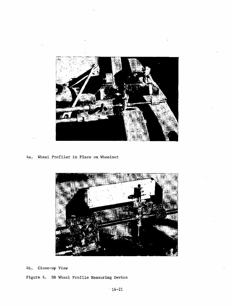
4a. Wheel Profiler in Place on Wheelset

4b. Close-up View

Figure 4. DB Wheel Profile Measuring Device

14-21

D I S C U S S I O N

Mr. Christianson: Christianson from Chessie System. Do I assume thateverything that you're talking about applies to tangent track?

Mr. Law (Clemson): The results that I've shown you apply for tangenttrack. The equations that I've shown you and the way in which those offsets, for example, enter for the curved track in exactly the same fashion although the values of the offsets may be somewhat different due to the different profiles that you'd see on a curved track as opposed to the tangent track.

Mr. Christianson: Does the absolute centerline, the rolling line offsettheory apply on the curved track?

Mr. Law: Yes. The way that the offset comes in is exactly the same forcurved track as it is for straight track. One thing, if you had identical rails left and right on the curved track and identical wheels, you still get a nominal rolling line offset that a free wheelset would adopt due to the combination of conicity and the curve radius. On top of that, you'd also have any dynamic offset, if you will, that would enter due to these changing railhead profiles as you go down the track.

Mr. Christianson: Now, what kind of a maximum axle yaw angle would youexpect on the tangent track? What have you experienced?

Mr. Law: It's on that order from what we've seen in the data that we got,yes.

14-22

M E C H A N I C A L S Y S T E M S M E A S U R I N G T E C H N I Q U E S F O R T R A C K G E O M E T R Y

Dr. Guenther Oberlechner, Ph. D

Plasser American Corporation 2001 Myers Road

Chesapeake, Virginia 23324

When the track is laid, it has to follow very tight design specifications for

the track geometry to achieve an optimum traveling speed between locations.

The maximum speed reachable is determined by the super-elevation and the

curvature, whereby optimum traveling speed between two locations demands

continuity in the design.

With moving traffic, the track deteriorates and reaches limits which do not

allow a safe train movement over the track anymore. In order to determine if

the track is still in a safe condition, its track geometry parameters have to

be measured. Hand measurements or track surveying are very time consuming and

labor intensive methods. They are, therefore, used only in special limited

cases. They are not useful for the determination of the overall condition of

the track and reflect unloaded track geometry. From the aforementioned, it

can be seen that in order to check the track condition economically, track

geometry measuring vehicles have to be used that continuoulsy measure the

track with speeds similar to train speeds and under loads similar to common

train axle loads.

In general, measuring cars provide information regarding gauge, super

elevation, twist, track surface, and track alignment. Other parameters, like

accelerations measured at various points of the vehicle, are speed dependent

and should only be used for evaluating track providing that an even measuring

speed can be maintained.

Three different types of geometry vehicles are known: High rail type geometry

vehicles, self-propelled railbound vehicles, and coaches pulled behind locomo-

15-1

tives as special trains or hooked onto the train configuration. High rail type

vehicles measure up to 25 mph, limited by the high-railing operation and are

predestined for main-lines with low train density and branch lines, since no

dead-heading is necessary. Normally, one operator handles the entire

measuring operation.

Self-propelled railbound geometry vehicles measure up to speeds of 80 mph,

depending on the detecting equipment they use. They are highly economical and

are used for main and branch lines. Normally two operators are necessary to

handle the driving and measuring part of the vehicle.

Coaches used as geometry vehicles can measure up to speeds of 130 mph and are

used mostly where high train density demands high measuring speeds. They have

high operating costs since a locomotive crew, in addition to the measuring

crew is needed and are therefore not recommended when testing branch lines.

If geometry cars have to be differentiated by their measuring devices, one can

distinguish between contacting and non—contacting sensors. Contacting sensors

are mechanical-electrical detecting devices using mechanical sensors

continuously touching the rail. These all-weather measuring devices are

either wheels, discs, or measuring swords, whereby the mechanical displacement

is converted into an electrical signal. Depending on the sensor, the speed

limit for wheels and discs is approximately 80 mph, for swords about 130 mph.

At higher speeds, due to inertia, there is no guarantee that the measuring

devices are continuously touching the rails.

Non-contacting sensing devices are proximity sensors, capacitive or magnetic

sensors, or photoelectric sensors. These devices allow measuring speeds up to

160 mph, but have complicated calibration procedures and cannot be used under

all-weather conditions. Since the topic of this presentation is "Mechanical

Measuring Techniques", let us discuss the various systems to measure the track

geometry parameters.

All mechanical systems are contacting ones, meaning that the sensor touches

the rail either on the surface, for parameters like rail profile or super

15-2

elevation, or on the side of the railhead, for parameters like gauge or

alignment. The horizontal or vertical displacement of the sensor is

electrically measured with linear transducers or potentiometers against a

reference, normally the stiff and torsion-free car-body frame. In some cases

on older cars, the displacements are converted directly into the needle

movement of a chart recorder via a linkage system and wires. In the case of

electronic measuring devices, an amplification system is used which allows the

zero-adjustment of the signal, and for calibration purposes, an adjustment of

the amplitude of the transducer signal.

As already mentioned, either wheels, discs, or swords are used as sensors.

These are continuously pressed against the rail via springs, pneumatically or

hydraulically. Adjustable pneumatically down- and side-pressured sensors are

advantageous over the other two systems since the air-cushion in the air-

cylinder guarantees a close contact to the rail even at high speeds and

through sharp curves. Systems using springs are subject to fatigue and

hydraulic systems are not flexible enough.

Wheels as measuring sensors are ideal in that they copy the profile of actual

railroad wheels, therefore touching the rail at the same points as locomotives

or cars do. They can vary in diameter from 11" to 28". On high measuring

speeds above 80 mph, due to inertia, a close contact between wheel and rail

cannot be guaranteed as the wheel sometimes jumps over track deviations such

as loose joints,! etc. The wheels need to be balanced very carefully to

provide optimum measuring results. Wheel diameters of 11" have shown

excellent results up to speeds of 90 mph; they are very easy to control with

down- and side-pressure, but have to withstand high revolutions when testing

with high speeds. The profile of the wheels are hardened and have a cycle

time of about 15000 miles before they need reprofiling. Since a wheel can be

reprofiled about three times without loosing too much of the flange material,

the lifetime of such a wheel is about 45000 miles, which characterizes it as

an economical measuring device. The advantage of the measuring wheel over

discs or swords is its independence from weather conditions. Since wheels are

heavy enough they work even in snow and mud conditions. One wheel can also be

used to simultaneously check the top and the side of the railhead. This is

not true for discs and swords, which only measure the side of the railhead

15-3

Since the Plasser Track Geometry cars, (the EM 80/110c and the EM 25 He Hy-Rail car) use measuring wheels as sensors, they are typical for mechanical-electric measuring devices. We will, therefore, discuss the measuring system used on these cars and how they detect the different track geometry parameters.

The -EM 80/110c Track Geometry car is a vehicle with five axles. (Figure 1) Two of the axles are loaded with approximately 18 tons; one of them is used for driving, the other, the rear running wheel, is used to measure superelevation and profile under load. The three remaining axles, located in the front, in the middle, and in the rear of the vehicle are pneumatically operated telescopic measuring axles which are used for gauge measurement, alignment, and profile. These three measuring axles can be lifted from the rails when the car is travelling or is on transfer. As a combination between the measuring axles and the loaded axles, the different parameters are measured as follows:

Gauge, as defined, is measured between the heads of the rails at right angles to the rails in a plane five-eighths of an inch below the top of the railhead. (Figure 2) The two wheels, mounted on the center telescopic measuring axle, whose halves are continuously side-pressured, join the rail exactly in the plane specified above. With worn out rails, this plane might vary. The measurement is done at the touching point of the train wheel and the rail, whereby the measurement reflects the true track gauge condition which also guides the train along its way. The adjustable pneumatic side-pressure allows to measure the gauge under pressures of up to 400 pounds. Since the ratio between side- and down-pressure is adjustable, a similar situation, as under a locomotic load, can be reached and loose rail mountings which would cause the rail to tip under load, can be detected.

The mechanical displacement of the two wheels, respectively the two halves of the telescopic measuring axle, is measured via a linear displacement transducer and then converted into an electrical signal, directly proportional to the geometry measurement.

and cannot be used for any measurement other than alignment and gauge.

15-4

MEASURING WHEEL

LOCATIONS FOR THE

DIFFERENT PARAMETERS

MEASURING AX LE S

P A R A M E T E R MEASURING W H E E L

A L I G N M E N T LEFT 1 2 3A L I G N M E N T RIGHT 1 2 3SUPERELEVATION O R C R O S S L E V E L 4G A U G E 2SU RF AC E IRREGULARITIES L E F T 4 2 3S U R F A C E IRREGULARITIES RIGHT 4 2 3VERTICAL ACCELERATION 4H O R I Z O N T A L A C C E L E R A T I O N 4DYNAMIC RELATIVE R O L L RATE A N G L E 4

FIGURE I15-5

M p - G A U G E

M£as“ rement

T a £ S C 0 P , C * * « * . *

In order to measure through switches, each wheel is rigidly connected to either a guide skid or a guide wheel on the other side of the telescopic measuring axle. (Figure 3) When the axle travels over the frog part of a switch, the guide pieces held by the guard rail guide the wheel safely over the open part of the switch and the gauge is measured throughout the entire switch without a reduction in measuring speed. The telescopic axle also clears spring loaded switches, and self-guarded switches since the wheel width is the same as standard railroad wheels.

For the alignment measurement, the front, the middle, and the rear measuringaxles are used, (Figure 4) whereby the axle base between front and rearmeasuring axle is exactly 31 feet. Since all these measuring axles areidentical, what is true for the middle measuring axle, where gauge ismeasured, is also true for the front and the rear measuring axle. Foralignment, the relative displacements of the three wheels, side-pressured toone rail, are measured against the stiff and torsion-free main-frame of thevehicle. The signals of the three linear transducers are combined in oneamplifier to the mid-chord off-set of a 31 foot chord line, according to the

A + Bformula: A plus B divided by 2 minus C, ( — — ” C), whereby A, B, and C arethe relative displacements of the front, the rear, and the middle axle, respectively. The output of the amplifier is converted later on by thecomputer from the 31 foot mid-chord off-set into a 62 foot mid-chord off-set in order to satisfy Federal Railroad Administration standards.

Also, in case of alignment, the ratio between the down-pressure and the side- pressure can be changed in order to reach similar conditions like under train loads. Since the sensors are mounted symmetrically to the car-body frame, car-body movement does not influence the measurements.

To measure the surface of the track, different methods are utilized. Longitudinal profile, as demanded by the Federal Railroad Administration standards is measured as mid—chord off-set of the 31 foot axle base between the front, and the rear measuring axle. (Figure 5) The same wheels which measure alignment are also used to measure longitudinal profile, whereby the cylindrical running surface of the wheel measures the top of the rail. Thethree vertical displacements of the three measuring wheels are detected by

15-7

MEASURING AXLE RUNNING THROUGH SWITCH

FIGURE 3

ALIGNMENTMEASUREMENT

x = ( - ^ - ) - c

MEASURINGAXLES

R E A R

cC E N T E R

AF R O N T

4END

V IE W

FIGURE 415-9

LONGITUDINAL PROFILE MEASUREMENT

15-10

linear transducers relative to the car-body frame and converted in the amplifier to the mid-chord off-set, similar as for alignment. Later in the computer, the 31 foot mid-chord off-sets are converted into 62 foot mid-chord off-sets. The adjustable down-pressure of up to 1000 pounds per wheel will cause the very weak and unsupported profile spots to be pressed down so that the measurements can detect track deviations caused by loads.

The second type of profile measurements are taken under an axle load of 18 tons. Since the loaded running axle, which has wheels with cylindrical running surfaces, is located asymmetrically between the measuring axles, an asymmetrical chord off-set over a 15.5 foot chord or over a 31 foot chord can be measured. (Figure 6) In both cases the track is loaded down and soft spots can be easily detected. These measurements, even if not requested by the Federal Railroad Administration, are of great importance for the evaluation of the track conditions.

The superelevation measurement is also taken under an 18 ton axle load. (Figure 7) A levelmeter, mounted to the car-body frame, continuously senses the super-elevation of this reference plane. Two correction feelers, mounted between this plane and the rear loaded running axle, whose wheels have, as mentioned before, cylindrical running surfaces, correct the level-meter measurements to the absolute track superelevation.

The twist or walrp measurements are derived by the computer from superelevation. Two superelevation measurements detected under an 18 ton axle load which are a constant distance apart are compared to each other. The distance between the comparing points can be varied.

Mechanical measuring systems always utilize wheels of either loaded or special measuring axles for profile measurement. This is also true for truck supported vehicles.

Gauge and alignment are measured as the horizontal displacement of either wheels, discs, or swords.

15-11

SURFACEIRREGULARITIESMEASUREMENT

(18 TONS)

(18 TONS)

FIGURE 6

SUPERELEVATIONMEASUREMENT

L E V E L M E T E R

L E V E L M E T E R

FIGURE 715-13

Discs are mounted slanted so that the disc rim touches the side of the railhead, 5/8 of an inch below the top of the rail. Otherwise they are side- pressured and guided in a similar manner like telescopic axles . and can run through switches without speed reduction. With discs, the self-guarded and spring-loaded frogs cannot be cleared without lifting the measuring devices.

Measuring swords are bars, mounted between the axles of a truck. They have specially hardened wear pieces mounted on them in a plane 5/8 of an inch below the top of the rail and are side-pressured from the truck frame against the side of the rail. The lateral displacement of the swords against this frame and the lateral displacement of the measuring frame against the vehicle frame are detected on three trucks and alignment established. Also, gauge can be detected as the horizontal displacement of the left and right measuring sword against the measuring frame by adding the fixed distance between the mounting points of the swords.

Although swords are able to measure up to 130 mph and clear switches without speed reduction, they have to be lifted off the track on spring-loaded frogs.

All measurements on mechanical systems are detected as horizontal or vertical displacements of rail contacting sensors. One of the biggest advantages of these systems, aside from that they are operable under all-weather conditions, is the ease with which calibration can be performed directly at the track site. The vertical or horizontal displacement can be simulated by applying a piece of known thickness between the top of the rail and the wheel measuring surface or between the side of the rail-head and the wheel flange. If a piece displaces the wheel, for example using one inch, and the linear transducer is adjusted for one (1) volt output, then each time a one (1) volt signal is measured it represents a track deviation of one (1) inch from zero. Since this is true for all parameters, the measuring system can easily be checked during actual testing and its accuracy verified. This simple calibration and checking procedure makes mechanical measuring systems most reliable, easy to troubleshoot, and does not demand highly skilled operators to make the system work. With mechanical-electrical measuring systems, tolerances of plus or minus 1/32 of an inch can be achieved for all parameters.

15-14

From what we have learned, mechanical measuring systems would be the most desirable ones if there were no speed limitation or mechanical system wear. Since the latter is limited to rail contacting sensors, they should not be overemphisized.

Finally, a few words on the influence of measuring speed and loads on measurements.

The rolling stock of each railroad varies in relation to the axle loads and axle bases. Therefore, to build a Geometry Measuring car which measures track simulating normal operating conditions is completely unfeasable. To use the railroad car and equip it with Treasuring devices is also impractical since conical wheels influence the measurement accuracy and cylindrical wheels provide poor ride qualities. Therefore, a compromise has to be made and from a Geometry car with known axle base and axle load the behavior of a railroad car has to be determined.

Tests have shown that the load of one axle is distributed over three ties, whereby the middle tie under the axle bears one-half of the load, and the other two ties each bear h, of the axle load. Since the axle base of a truck is never less than six (6) feet, the two axles of the truck never influence the maximum rail deflection of the other axle. This means that the axle distribution is insignificant.

The relation between axle load and track deflection is the same as known from the soil mechanics whereby the settlements due to the load distribution of the ties normally stays in the elastic range. (Figure 8) Tests have shown that on a normal supported track the elastic deflection of one track spot under various axle loads is relatively little compared to track errors. An axle load of twelve (12) tons caused an elastic deflection of 2.1 millimeters (0.08 inches), and an axle load of 25 tons, a deflection of 3.4 millimeters (0.13 inches). (Figure 9)

The influence of the axle load for gauge and alignment on tangent track is

insignificant, as long as the rail fasteners and the tie conditions are

satisfactory. Lateral forces are experienced only in curves which causes the

15-15

LOADK P /C M 2

S E TTL E M E N T

FIGURE 815-16

oj ro

0 2 4 6 8 10 12 14 16 18 20 22 242628 301

><ur

" d

MLCTREV

)AIACAT

DEIK101

12D

Si

:t A>-- T

:leT--ILC

i

—i—i

DACiiiiiiiiii

—) 251iiiiiiiii

i

—

> [Dx G/3\P BELOW TIEL

_i— ii ii-Imm/ lot i

_ L

—i— i i—t1i !}1.3MMr **cU

MMSETTLEMENT

FIGURE 915-17

gauge to widen, but leaves alignment uninfluenced, since the track is evenly side-pressured.

High speeds increase the axle loads which can be compensated for by introducing a speed factor. Depending on the speed changes from 16 mph to 125 mph, the factor increases from 1.01 to 1.30. (Figure 10) Since the difference between the deflection of two axle loads, where one is 10 per cent higher, is only 0.1 millimeter (0.004 inches), the speed influence on measurements is insignificant. As proof of the above, Professor Eisenmann showed that a locomotive with 21 tons axle load, traveling at 125 mph (200 km/h), caused only a 0.005 inch (0.12 millimeter) larger deflection than when traveling at 6

mph (10 km/h). (Figure 11)

As shown above, from measurements taken with a single axle of a known load and at a known measuring speed, measurements for various axle loads and traveling speeds can be predicted.

Since the speed limitation for mechanical measuring systems is of no consequence, the preference is given to Track Geometry cars using mechanical systems.

15-18

SPEEDADJUSTMENT

FACTOR

V-MPHAS PER

PROFESSOR SCHRAMM

INPRACTICE

5 0 %

16 1 . 0 3 I.OI

3 0 1 . 0 9 1 . 0 5

4 5 1. 1 9 1. 1 0

6 0 1 . 3 0 1. 15

8 0 1.41 1 . 2 0

9 5 1.51 1 . 2 5

n o 1 . 5 7 1 . 2 7

1 2 5 1 . 6 0 1 . 3 0

FIGURE 1015-19

TESTBY

PROFESSOREISENMANN

RAIL T Y P E - S 49 K - B A L L A S T F A ST EN ER

FIGURE II

DISCUSSION

Mr. Caldwell: Caldwell from CN Rail Research. You show on your super -relevation a device you referred to as a tilt meter. Is the system compensated or does it respond to lateral centrifugal accelerations?

Dr. Oberlechner: There's a compensated acceleration system similar to theone used on the Department of Transportation cars in the States.Mr. Dibble: Thank you very much. I'd like to make some announcements

and before that, Dr. Klaus Riessberger, Head of Research at Plasser in Austria has a few slides he's like to show in reference to the first two papers this morning.

15-21/15-22

INERTIAL AND INDUCTIVE MEASUREMENT TECHNIQUES FOR TRACK GEOMETRY

Ta-Lun Yang Edward D. Howerter Richard L. Inman

ENSCO, INC.5408A Port Royal Rd. Springfield, VA 22151

1. IntroductionThe Federal Railroad Administration (FRA) of the Department of Transportation (DOT) has sponsored the development of automated track geometry measuring cars since 1966 for supporting track inspection and rail research activities. Several generations of measurement instrumentation and data processing capabilities have evolved in the development process. Currently under the Automated Track Inspection Program (ATIP), the FRA Office of Safety operates three track geometry survey vehicles; these are T-2 (with T-4 as its support vehicle), T-3 (with T-l as its support vehicle) and T-6 (operated without a support vehicle). These survey vehicles are operated routinely on a prescheduled basis to cover approximately 70,000 miles of track annually. Electronic sensing devices and data processing equipment installed in these vehicles measure track geometry at speeds up to 120 miles per hour, record the data on magnetic tape, display the measurements on oscillographs and produce an exception report in accordance with the Federal Track Safety Standards.

A fourth track geometry survey vehicle, T-10, is currently under construction and scheduled to join the FRA ATIP fleet in 1981. T-10 is based on a self-propelled coach, the Budd SPV2000, and incorporates the latest generation of inertial and inductive measurement techniques as well as the associated real-time digital processing algorithms.

16-1

ENSCO supported the FRA in the development and the operation of the current ATIP track inspection fleet and is also responsible for the design and the fabrication of the latest instrumentation used in T-10. This paper presents a brief description of the inertial and inductive measuring concepts and data processing techniques employed in all of the FRA track survey vehicles. Since implementation details differ somewhat among these vehicles, the latest version as used in T-10 is given whenever specific examples are provided in this paper. If the reader is interested in the instrumentation or data processing capabilities installed in a particular FRA track survey vehicle, any one of the authors at ENSCO will be able to furnish more detailed information.

2. BackgroundInitial layout and construction of railroad tracks rely on conventional survey techniques to establish earth-based references. Subsequent surveys of track geometry are generally for the purposes of identifying critical geometrical defects that are safety hazards, providing data to calculate and prescribe the proper repair, evaluating the service performance of the track and planning long-range maintenance activities.The instrumentation and data processing equipment used in the FRA track geometry survey vehicles is designed to acquire the data at normal track speed from a moving vehicle to meet the general purposes described above. Specifically, tlhe identification of track geometry defects must be done in accordance with the format and the allowable thresholds provided in the Federal Track Safety Standards.

Gage measurement is made in terms of the absolute distance between the inner faces of the two rails. No additional external reference is needed to establish the measurement. The inductive technique to measure truck- to-rail distances was chosen for several reasons. A non-contact transducer is preferred because of the high test speed involved. Among the various non-contact proximity sensing techniques, a high-frequency magnetic approach requires a relatively small transducer and is reasonably insensitive to harsh environmental conditions. The small size of the

16-2

sensor allows it to be servo-controlled to maintain its distance from the rail so that the measurement is always within the linear range of the transducer, and, to focus on the FRA-specified measuring point of 5/8" below the surface of the rail.

The truck-to-rail measurements made with the inductive transducers are also used as a part of the alignment system which determines the smoothness of each rail in the lateral direction. The general interest in alignment is in its spatial frequency content which could induce vehicle lateral dynamics. Because of typical rail vehicle construction, alignment deviations from a wavelength of a few inches to several hundred feet are of interest. The significance of the long wavelength components generally begins to diminish at 150 feet for speeds up to 90 mph and at 200 feet up to 120 mph. The Federal Track Safety Standards defines maximum allowable alignment irregularities in terms of deviations from uniformity measured in a 62-foot midordinate-to-chord offset (MCO). The use of a pseudo-inertial measurement reference provides both the broad range of wavelength coverage needed for track-train dynamic research and the 62' MCO (as well as MCO's of other chord length) required for checking compliance. An accelerometer, after appropriate processing, measures the oscillatory movements of the truck lateral to the track centerline. The processed output of the accelerometer is sometimes referred to as the pseudo-space curve for the truck path. A pseudo-space curve can be interpreted as the inertial trajectory of the truck with its long wavelength components and the d.c. component removed. The left and right side truck-to-rail distances and the servo-positions are combined with the pseudo-space curve of the truck to form the pseudo-space curve representing the alignment of each rail.

The general interest in rail surface profile is over a broad range of wavelength pertinent to vehicle dynamics, similar to the case of rail alignment. Since the running wheels in a measuring vehicle provide natural loaded contact measuring points, the vertical movements of a wheel combined with a pseudo-vertical inertial reference would me£t the

I6 - 3

profile measurement requirements. Two vertically mounted accelerometers are used over the measurement axle to establish the pseudo-inertial references for the left and the right rails.

Superelevation (often referred to interchangeably as crosslevel), is measured with respect to the local horizontal plane, therefore, a local vertical reference must be established on the moving vehicle. A true inertial attitude reference, such as a stabilized platform used in spacecrafts, does not meet the requirement because the local gravitational vector is not fixed inertially. For this reason, an inclinometer mounted on the floor of the car across the measuring axle is used as the basic transducer to sense the tilt angle of the floor relative to the gravitational vector. Complex filtering and compensations using outputs from two rate-of-turn gyros and truck-to-carbody displacement transducers are needed to eliminate errors in the measurement due to vehicle dynamics. Tilt angle of the track, which converts directly to superelevation, is then obtained by measuring the axle-to-carbody roll angle.

Vehicle speed, distance, track curvature and track location measurements are also made by the survey vehicles to provide location reference and to furnish necessary inputs to the processing algorithm. With the nominal sample rate of one foot, the magnetic Automatic Location Detector (ALD) system can provide correlation within +6 inches between track location and geometry data. Curvature and curvature rate data are analyzed by onboard software to detect transition points between tangents, spirals and curves so that appropriate standards can be applied.

3. Measurement System Description3.1 System OverviewThe Track Geometry Measurement System (TGMS) has the capability to measure gage, curvature, crosslevel, warp, profile and alignment of the track.The conversion of the transducer signals to the measurement of the track parameters is performed primarily in the onboard computer by digital algorithms. The general approach for all of the basic parameters is to

16-4

condition the raw transducer signals with an appropriate filter whose frequency response characteristics are designed to mate with the digital computations performed in the onboard computer. The conditioned transducer signals are then digitized at a constant distance interval of one foot.

Each of the conditioned transducer inputs is then examined by a specially- designed digital algorithm to detect signal fault conditions. The conditioned transducer signals are stored on a digital magnetic tape which serves as a permanent record.

The digitized sensor signals are then processed through digital filters whose frequency response characteristics are matched with their analog counterparts. The hybrid filter formed by combining the effects of both the analog and the first stage of digital filtering yields sensor signals whose phase characteristics are invariant with regard to distortion normally introduced by variations in vehicle speed and direction of travel.

These processed sensor signals are then used to calculate the necessary track geometry parameters required for exception detection and display. Track geometry parameters are scaled and displayed on strip chart recorders for the track inspectors and the system operator. These track geometry measurements are distance synchronized to a common location reference even though the transducers are mounted on different locations within the vehicle. .The strip charts are distance based so that one mile of data is displayed on approximately 18 inches of paper regardless of speed. Exception report is printed on a line printer in which each detected exception to the Federal Track Safety Standard is reported with respect to its location on the track. The measurement of traversed distance is accomplished by an axle-driven tachometer (optical encoder) which also controls the computer for distance-based data acquisition. Vehicle speed is calculated from time elapsed between two consecutive distance interrupts through the use of a highly accurate, crystal controlled oscillator as a time base.

16-5

A simplified system schematic is shown in Figure 1. The dependency between measured parameters and input transducers is shown in Figure 2.It can be seen that several measurements are generally required to obtain each of the track geometry parameters and that each transducer serves as inputs to many geometry parameters.

3.2 GageThe earliest gage measurement system used capacitive, non-contact proximity sensors. These sensors were mounted parallel to each rail, facing the inside of the railhead in the shadow of the wheel flanges. The lateral positions of the sensors were fixed relative to the wheels so that the range of each sensor must cover 0.2" to 2.0" in order to accommodate typical lateral excursions of the wheels. These sensors were retractable vertically by a remote signal to clear switches and road crossings.

Adding the two conditioned sensor signals to the distance between them produced a measurement of track gage.

The main weaknesses of the capacitive system are that at a range of two inches, the response is quite nonlinear and that the electro-static field is subject to fringing and distortion due to grass, debris, water and snow.

A servo-magnetic gage system was developed to overcome the problems inherent in the capacitive system. This system also measured the relative position between the truck and each rail, but utilized an inductive transducer, servo-controlled to maintain a nominal distance from the rail to keep the sensor well within its linear range. The magnetic sensing technique is relatively immune to all but the most severe weather conditions. The sensor is retractable vertically, and is also equipped with a relatively inexpensive breakaway support to protect the measurement coil. Most recent sensor arm design employs a spring-loaded resilient arm holder which allows sensor to deflect and return when hit by a track obstruction.

16-6

16-7

PROGRAMINITIATION

OPERATIONSCONTROL

TRANSDUCERS

RAW ANALOG SIGNALS

______ *______ANALOG

PROCESSING

PROCESSED ANALOG SIGNALS

. +A/D

CONVERTER

DIGITAL SIGNALS________

DIGITAL COMPUTER

CLOCK-►TIME BASE> «-------

+ " : ' . i - + _PRINTER/PLOTTER

D/ACONVERTER

TAPEDRIVES

PROGRAM OR DATA TAPES

DISCPROGRAM

« -► OR DATA STORAGE

EXCEPTIONREPORT

TRACK GEOMETRY

STRIP CHARTS

Figure 1. Track Geometry System Schematic.

16-8

Figure 2. Track Geometry Parameter Transducer Dependency.

j Pro

file

i

Acc

eler

omet

erI Si

ght__

___

Allg

nom

eter

A

ccel

erom

eter

Figure 3 shows the basic measurement concept. An error signal from each magnetic sensor is fed into a servo-control loop to maintain a nominal distance of approximately 1/2 inch from the gage side of the railhead. The relative position of each sensor is measured by a linear displacement transducer, summed with the error signal, conditioned and digitized by an onboard data collector system.

The digitized sensor inputs are then examined by a specially designed digital algorithm to detect out-of-range and lack-of-activity fault conditions. After being stored in cyclic arrays to synchronize the measurements of track gage with the remaining track geometry parameters, the input voltages are summed and added to an offset number to yield the final measurement of track gage. The resultant measurement of track gage is then used for exception detection. Finally, the measurement of track gage is scaled for output display.

3.3 CurvatureThe curvature system utilizes five transducers which consist of a yaw-rate gyro mounted in the carbody, two displacement transducers measuring the relative lateral distance between the leading truck and the carbody, a displacement transducer measuring the relative lateral distance between the trailing truck and the carbody, and an optical encoder.

The yaw-rate gyro is used to supply a voltage proportional to the yaw rate of the carbody. This voltage is conditioned by an analog low-pass filter with a gain and zero'offset. The frequency response of the analog filter is given by

B(s)

Q ls + m i

where in5= -- ~ 0.76 rad/sec,l 2 1 7

16-9

16-10

Figure 3. Gage System Sensor Configuration

8 = jfi,

a = Ai,

and fi = radian frequency, rad/sec.

The magnitude response of this analog filter is shown in Figure .4 for V = 9 mph and 80 mph. It is significant to note that the fixed time frequency corner implies a variable spatial frequency corner which is dependent on the speed of the vehicle. The filtered signal is digitized at a sample interval of one foot. A debias command can be enabled by the oper ator when the vehicle is stationary, this effectively eliminates any residual bias in the output of the yaw rate gyro.

The debiased signal is then processed by a digital filter whose mathematical form is given by

9 . .T n T .1 t 1 %

„ 2 _ 2 -iC(z) = $----=-S------£—ft T.

1 i

where z = z transform notation for a single sample delay.

= is the time interval between the current, -ith, and the previous, (£ - l)th, data samples.

16-11

MAGNITUDE,

db

rel.

0.0001 O.OOIr u i i q u i i N C Y , c y / r t

0.01 0.1 l . o

Figure 4. Magnitude Response of First Order Analog Filter, B(s).

This bandpass filter has variable spatial frequency characteristics, as shown, in Figure 5, similar to those of the first order analog filter,B(s). The magnitude response characteristics of the first order hybrid filter formed by the analog filter, B(s), and the digital filter, C(z) , is shown in Figure 6. The first order hybrid filter has a spatial frequency characteristic which is independent of the vehicle speed and direction.An extremely close approximation is used in the actual implementation of C(z) to facilitate efficient numerical calculations in the computer.

The yaw-rate gyro output, after the hybrid filter, represents the temporalrate-of-change of vehicle heading d<b /dt with a high-frequency cutoff

Owhich is constant in spatial frequency. In order to convert this measurement to track curvature, we note that:

A<f)a

Ax

A<p<At Ax At

A*r Qwhere 1\^~ = the change in the heading of thecarbody over the distance interval, Ax3

Ad)a

At the change in the heading of the carbody over the time interval, At = T.

and AxAt the average speed of the vehicle

over the distance interval, At

16-13

MAGNITUDE, d

b rel.

(1. 110(1 II . nil IIIM'IJIII.NCV. « y / n

ll.lll 0.1 1.0

Figure 5. Magnitude Response of First Order Digital Filter, C(z),

MAGNITUDE, db rel.

HtliQllliNCY, cy/fl

0.0001 0.001 0.01 o.|

This implies that C(z) must be divided by velocity, or equivalently, mul

tiplied by the time interval T ., to obtain the change in the heading of

the carbody over the unit sample distance interval. Since the carbody yaw

rate as seen by the gryo contains oscillatory yaw motions of the carbody

relative to the truck which are not directly representative of track ge

ometry, corrections must be introduced.

Three displacement transducers are used to supply voltages proportional to

the lateral translation of the trucks relative to the carbody. These

voltages are conditioned by an amplifier and are digitized in conjunction

with the other transducers each foot of vehicle travel. The signals from

the two displacement transducers located on leading truck, are combined to

yield the front carbody-to-truck lateral translation. The third displace

ment transducer located on the trailing truck, yields the trailing carbody-

to-truck lateral translation.

The two measurements of lateral translations of the trucks relative to the

carbody provide the measurement of the osciallatory motions of the carbody

and are subtracted from the measured yaw rate per unit distance.

This corrected yaw rate A<J> /A is then low-pass filtered to yield a measureq . <£

of track curvature. The digital filter to evaluate track curvature is

given by

D(s)1 1M N

Z-K - 1) ( / -

where K = 38,

M = 2K + 1 = 77,

L = 58,

and N = 2L + 1 = 177.

16-16

The values of K and L given in the above equation are selected to deem-

phasize the undesirable periodic behavior introduced into the measurement

of track curvature inherent in bolted rail track design.

The magnitude response of this filter has a constant wavelength charac

teristic and is shown in Figure 7.

The rate of change of track curvature is also calculated by a digital

filter. Track curvature and rate of change of track curvature are used

in a curve analysis algorithm to detect curve transitions and type,

i.e., tangent, spiral and curve, for use in determining which thresholds

to apply to the track parameters in exception reporting.

3.4 Crosslevel

Crosslevel was initially measured using a vertical gyroscope, four ca

pacitive proximity sensors and two displacement transducers. The ver

tical gyro measured carbody roll angle. The carbody measurement was

referenced to the truck frame using the displacement transducers, and

further, to the rail by the proximity sensors. This system was subject

to significant errors due to slaving and de-slaving the vertical gyro

and large uncompensated dynamic inputs.

The Compensated Accelerometer System (CAS) was developed in the 1974 -

75 period. In the CAS, an accelerometer used as an inclinometer, paired

with a roll rate gyroscope, became the primary roll angle measurement.

Compensations for yaw rate and lateral accelerations were included. The

original CAS and a subsequent improvement employed a complex multiple-pole

analog computer to perform the processing. The complex processing scheme

has now been implemented in T-10 with digital algorithms which eliminates

most of the remaining errors inherent in analog computers. The T-10

crosslevel system utilizes four transducers in addition to the debiased

yaw rate gyro signal and time-between-samples (TBS) datum used in the

track curvature algorithm. These additional transducers consist of a

carbody mounted inclinometer, a roll rate gyro, and two displacement

16-17

MAGNITUDE, db rel.

0.000l 0.001HUiQIJliNCY, cy/l't

0.01 0.1 1 .0

Figure 7. Magnitude Response of Track Curvature Digital Filter, D ( z )

transducers. The transducer mounting configuration for the crosslevel

system is shown schematically in Figure 8. The carbody mounted incli

nometer is used to calculate the low frequency components of the carbody

roll angle with respect to gravity. Compensation factors are included

to counteract the accelerations sensed by the inclinometer due to: cen

trifugal acceleration of the vehicle, motion of the inclinometer about

the yaw center of the vehicle, roll .accelerations of the carbody about

the track and about its own roll center, and lateral translations of the

vehicle. The carbody mounted roll rate gyro is used to calculate the

high frequency components of the carbody roll angle with respect to

gravity. The two displacement transducers are used to measure the rela

tive roll angle between the carbody and measuring axle.

The voltage produced by the inclinometer is conditioned by an analog

low-pass filter with a gain and zero offset. The frequency response of

this analog filter is given by

F(s)a 2 + b 2

(s + a)2 + b 2

where a — SL2

b = A - sJ n2

& = 1/2,

and 6.10 rad/sec.2 \ 2 1If/

The magnitude response of this analog filter has a fixed time frequency

corner and therefore a variable spatial frequency corner which is de

pendent on the speed of the vehicle. After being processed by this

analog filter the signal is digitized at a sample interval of one foot.

16-19

For the purpose of profile and alignment calculations, the digitized signal is processed by a digital filter which mates with the analog filter given above to form the second order hybrid processing filter.

The digital filter is given by:

G(z) = T + Tn n- i

aTn

Vsin bT n

sin b(T + T ) _________ n n- isin bT sin bT , n n- 1

-aTn- i

sin bTn- i

where a and b are defined above and T and T are the time intervalsn n- i

between consecutive data samples for the current and previous sample

interval, respectively.

The magnitude response characteristics of the second order hybrid filter

formed by the analog filter, F(s) and the digital filter, G(z) , is shown

in Figure 9. it should be noted that the second order hybrid filter has

spatial frequency characteristics which are independent of vehicle speed

and direction.

The digital portion of the second order hybrid filter is rescaled and

multiplied by T ^ l to yield a short mid-chord offset (MCO) of the

acceleration signal. This signal is used later in profile and alignment

calculations to compensate for errors introduced by carbody roll motions.

For the purpose of obtaining the low-frequency roll angle of the carbody,

the digitized inclinometer signal is processed by a first order low-pass

filter. This low-pass filter is designed to match the effects of the

16-21

MAGNITUDE, db rel.

I'UliQlllINCY , i:y/ I*I

0.0001 0.001 0.01 0.1 1.0

Figure 9. Magnitude Response of Second Order Hybrid Filter.

first order filter applied to the roll rate gyro signal which provides the

high-frequency portion of the roll angle. The form of this low-pass filter

is given by

H (s)

ni

s + Q,1

where = --- ~ 0.76 rad/sec.l 2 17

The magnitude response of this filter has been discussed in Section 3.3.

Two types of errors are contained in the signal due to yaw motions of the

car, these are the centrifugal acceleration and the acceleration sensed by

the inclinometer due to movement about the yaw center of the vehicle.

Correction terms are obtained using the yaw rate gyro input. The correc

tion terms are combined and processed by a second order low-pass filter.

This low-pass filter is designed to match the effects of the second order

filter applied to the inclinometer signal. The form of this filter is

given by

a 22

B = ---------------2 s2 + s -f ft 2

2 2

where ^ ----- s 0.19 rad/sec2 2 17

These filtered correction terms are applied to the filtered inclinometer

signal which is then low-pass filtered to remove the remaining error in

troduced by the pure lateral translation of the carbody. The form of this

low-pass filter is given by

£1 2fl 2 £2 / 1 2 3 2 3\ 1 2 2 3 1 3/

H (s) ----------------- 7—“------------ r--------3 n n 2 (s2 + n s + n 2)

1 2 ' 3 3 /

16-23

10 5where ft = --- s 0.19 rad/sec

3 o 19

The form of H (s) is designed to yield a composite filter given by3

H(s) = H (s)H (s)H (s)1 2 3

which has a constant time corner approximately two octaves below the lat

eral rigid carbody natural frequency (typically around 1.25 Hz).

The magnitude response of the composite filter, H(s) , is shown in Figure 10 for V = 9 mph and 80 mph.

To obtain the high frequency components of the carbody roll angle the roll

rate gyro signal is processed by a filter, P(s) , whose frequency response

is complementary to H(s) and is related to HCs) by the following equation

H(s) + sP(s) = 1

The filter P(s) is formed by a composite of P (s) given byl

P (s) =l

ftl

s + ftl

where ^ - ~ 6.10 rad/secl 217

which is performed by the analog circuitry and

P (s) 2

s5 + gs1* + r\s3 + ks2 ft (s2 + ft s + ft 2) (s2 +89. + ft 2)

1 2 2 3 3

16-24

MAGNITUDE, db rel.

0.0001 0.00 1I'ltliQllliNCY , c y / l l

0.0! 0.1 1.0

Figure 10. Magnitude Response of Composite Low-Pass Filter, H ( a ) .

where ^ = £2 + £1 + Q,1 2 3

n = f i 2 + ft ft + ft ft + ft ft + ft 22 3 2 1 2 1 3 3

and k — (Q, + ftjft2 -fftftft -f ft 2 f ft f J2 J1 3 2 1 2 3 3 1 2

The composite filter is given by

P(s)s = .P (s)P (s)l 2

s5 + go1* + ns3 + k s z_______

s5 + gs* + ris3 + ksz + es + y

where g = ft ft fft ft -f ft ft + ft ft j2 3 2 3 1 2 1 3

and y = ft ft 2ft 21 2 3

The magnitude response of the composite filter P(s)s is shown in Figure 11

for v = 9 mph and 80 mph.

The data processed by filters H(z) and P(z) are then combined to yield

the carbody roll angle, 0 , over the pass band of interest. The two

displacement transducers are then used to calculate the roll angle between

the carbody and the track, 0 . The track roll angle 0 = 0 + 0 , is

then scaled to a reference baselength to yield track crosslevel.

To calculate deviation from design in spirals and curves the crossleveldata is processed by a high-pass filter given by

16-26

•T« qP

‘HQfllINDVT-!

0.0001 0.001 0.1nu-ijm-NCY, cy/n

o.oi 1.0

Figure 11. Magnitude Response of the High-Pass Filter, P ( s ) s .

J -J- 1- 3

where J = 61 feet

The magnitude response of Q(z) is shown in Figure 12.

3.5 Profile

The original profile system, like gage, utilized capacitive sensors located

at the front, middle and rear of a 14.5 foot beam. These sensors measured

the vertical displacements of the rail from the beam. Subtracting the

midpoint measurement from the average of the front and rear measurments

yielded a 14.5 foot mid-chord offset measurement of profile. This profile

system suffered from the same inaccuracies and weather restrictions as the

earlier gage system.

The first inertial profilometer used on the FRA inspection cars was based

on a sensor developed by the Electromotive Division of General Motors.

The sensor consists of a classic spring-mass system mounted on the truck

with acceleration and displacement measurements of the mass. the original

sensor was rather bulky and weighed approximately 90 pounds. Subsequent

improvements resulted in an order of magnitude reduction in weight and a

significant size reduction. The latest profilometer system, used in T-10

eliminated the truck-mounted spring-mass sensor altogether; an inertial

reference is established in the carbody instead.

The T-10 profile system utilizes two inertial transducers in addition to

the transducers used in the crosslevel and curature systems. These trans

ducers consist of two vertically oriented carbody mounted accelerometers

located over the two carbody-to-axle displacement transducers. The pro

file system transducer arrangement is shown schematically in Figure 13.

16-28

MA

GN

ITU

DE,

db

re

l.

I'KIiQllliNCY, cy/ft

0.1)001 0.001 0.01 0.1 1.0

Figure 12. Magnitude Response of High-Pass Filter, Q ( z ) .

16-30

Figure 13. Profile System Sensor Configuration

The carbody mounted accelerometers are used to provide an inertial refer

ence and the displacement transducers are used to yield a measurement from

the inertial reference to the rail to obtain the measurements of individual

rail profile. The voltages produced by the accelerometers are conditioned

by an analog low-pass filter with a gain and zero offset. The frequency

response of this analog filter is the same as F(s) discussed in Section

3.4.

Following the digitization of the conditioned accelerometer signals they

are processed by a digital filter whose frequency response is the same as

G(z) discussed in Section 3.4. These operations produce a basic datum

whose spatial frequency characteristics are nearly independent of vehicle

speed and direction. Recall that the acceleration signal becomes a short

mid-chord offset (MCO) representative of the input parameter after it has

been processed by the filter characterized by G(z) . These basic data are

then compensated for the relative roll angle between the carbody and the

track to reference the measurement of profile perpendicular to the plane

formed by the tops of the railheads. The basic datum from the accelerome

ters is also adjusted with a gravity and centrifugal acceleration correc

tion. These basic data are then combined with the corresponding short

MCO's of the inertial references from the carbody to the track calculated

from the displacement transducers. The calculations discussed above are

completed for both sides of the vehicle and then a compensation is per

formed to correct for the fact that the transducers are not mounted di

rectly over the rail.

The next step in the processing is to convert the short MCO's to a MCO

with a longer baselength or to a pseudo-space curve. This is accomplished

by processing the short MCO data through a digital filter with the appro

priate frequency response. The filter for conversion from a two-foot MCO

to a 62-foot MCO is given by

U(z)2

16-31

where K = 15,

and M = 2K + 1 = 31.

The magnitude response of the digital filter is shown in Figure 14.

The MCO's with the 62-foot baselength calculated in the previous equation

still retain undesirable long wavelength information which should be re

moved. The long wavelength portion which passes through JJ(z) can be repre

sented by the signal that passed through a filter having an additional

order of low-pass than that of U(z) . This filter is given by

where L = 41

and N = 2L + 1 = 83.

A composite filter is then formed to perform the conversion and long-wave

length removal simultaneously. The composite filter is given by

W(z) = U(z) - V(z).

The magnitude response of the composite filter is shown in Figure 15.

If we separate the total effect of W(z) into a conversion operation and a

high pass operation, then, the high-pass portion of the operation can be

expressed as a filter given by

r, , _ K(z) = , V(z)U Z J ~ U(z) ~ U(z)

16-32

MAGNITUDE,

db rel

.

riU-Qlll-NCY, cy/fl

0 . 0 0 0 1 0 . 0 0 1 0 . 0 1 0 . 1 1 . 0

Figure 14. Magnitude. Response of Short-To-Long Mid-Chord Offset Conversion Filter, U(n).

MAGN

ITUD

E, db

, rel.

luinqiiKNCY, t v / f t

0.0001 0.001 0.01 0.1 1.0

The magnitude response of Xfz) is, therefore, given by the difference of

the magnitude responses of W(z) and U(z) and is shown in Figure 16. The

profile output of the analog and digital filters represent deviations from

average profile measured in the form of a 62' MCO. Different filters can

be substituted for W(z) to obtain MCO's of other chord lengths or a pseudo

space curve.

3.6 Alignment

The early alignment system utilized the same capacitive sensors as those

used for the profile systems yielding a 14.5 mid-chord offset alignment

measurement. The development of an inertial alignment system took several

years of analysis and many iterations of unsuccessful experimentation.

The first successful inertial alignment system was installed in T-6 which utilized a foam-isolation technique for mounting accelerometers. The T-10

alignment system design is identical in concept to the T-6 system.

The T-10 alignment system basically consists of an accelerometer mounted

on the instrumented beam assembly to provide an inertial reference and the

gage sensors to yield measurements from the inertial reference to the

individual rails. The alignment system configuration is shown schemati

cally in Figure 17. The track roll angle calculated from the crosslevel

system is used to compensate for the variations of the alignment acceler

ometer orientation with respect to gravity and for the accelerations in

duced due to the fact that the alignment accelerometer is not in the plane

of measurement.

The voltage produced by the accelerometer is conditioned by an analog low-

pass filter with a gain and zero offset. The frequency response of this

analog filter is the same as F(s) discussed in Section 3.4. Following the

digitization of the conditioned accelerometer signals it is debiased by a

digital filter whose frequency response is the same as R(z) discussed in

Section 3.5.

16-35

MAGNITUDE, db rel.

l:ltl:i)lfl:fJCY, cy/fl

(1.0001 0.001 0.01 0.1 1.0

Figure 16. Magnitude Response of Digital Filter, X(z).

16-37

Figure 17. Alignment System Sensor Configuration

Following the digitization and debiasing of the conditioned accelerometer

signal it is processed by a digital filter whose frequency response is the

same as G(z) discussed in Section 3.4 These operations produce a basic

datum whose spatial frequency characteristics are nearly independent of

vehicle speed and direction. Recall that the output of the digital filter

characterized by G(z) is a short mid-chord offset (MCO) representative of

the input parameter. This basic datum is then adjusted to compensate for

the fact that the inclinometer is sensitive to lateral accelerations in

duced by gravity component due to roll angle and by roll acceleration

because the accelerometer is not mounted in the plane connecting the

individual railheads. The signals from the gage sensors are then used to

calculate a short MCO of the distance between the inertial reference and

the gage side of the railhead. The short MCO calculated from the indi

vidual gage sensors are combined with the inertial reference provided by

the corrected alignment accelerometer to yield a short MCO of the align

ment of each rail.

The next step in the processing is to convert the short MCO of the indi

vidual rail alignments to a MCO with a longer baselength or a pseudo-space

curve. For conversion to a 62'-MCO, the short MCO is processed by a digi

tal filter whose frequency response is the same as U(z) discussed in

Section 3.5. These MCO's with the 62-foot baselength still retain the

undesirable lopg wavelength information which should be removed. This

long wavelength information is removed by low-pass filtering the short

mid-chord offset data with a filter whose frequency response is the same

as V(z) discussed in Section 3.5. Finally, the filtered data from JJ(z) and

are combined to yield the composite effects of W(z) as discussed in Section

3.5. These final data values represent alignment deviations from average

measured in terms of a 62'-MCO. A pseudo-space curve or MCO's of other

baselengths can be obtained similarly by substituting the appropriate

digital filter for W(z), 4

4. Advantages and Disadvantages of the System

The use of pseudo-inertial references for profile, alignment and cross

level measurement provides the uniform accuracy needed for the full

16-38

range of spatial frequencies pertinent to vehicle dynamics. Mid-chord

offset measurements of any chord length, including the 62-foot chord,

can be obtained easily from the inertial-based measurements.

The use of hybrid analog/digital processing schemes allows the reproduc

tion of accurate track geometry measurements independent of vehicle

speed or direction of travel. The use of digital data processing

techniques also allows the synchronization of all measured parameters

to a common track location reference even though the transducers are

mounted at different locations of the vehicle and various distance de

lays are introduced by processing algorithms.

The non-contact magnetic sensing technique permits the measurement of

gage and alignment from the 5/8" point below the rail head. This

system is not affected except for the very extreme weather conditions.

The use of load carrying wheels for rail surface measurements (profile

and crosslevel) and non-contact transducers near a wheel-rail contact

point for line measurements (alignment and gage) makes it possible to

measure track geometry under the load of the measuring vehicle and at

the highest speed permitted by the track.

The major disadvantage of an inertial-based system is the inability to

measure at low speeds. The profile and alignment systems will have

degraded measurement accuracties below 15 mph, the measurement accura

cies are not to be relied upon below 5 mph. The curvature measurement

is accurate down to approximately 2 mph; gage and crosslevel measurements are the only two that remain accurate to 0 mph.

16-39

DISCUSSION

Mr. Sweet: Larry Sweet from Prinction. When you're doing your processingof your signals, are you using just the complementary filter type techniques which you allude to in your paper or do you use other estimation techniques to account for noise in signals?

Mr. Yang (ENSCO): The filter shapes that you see are the shapes of thefilter we used. The actual filters I've written in the paper are the theoretical filters. What we have implemented is a numerical approximation of those filters, the response is very, very close. If you overlay them, you can't even see the difference. And those are the only filters. There are no additional filtering done on the signals.

Mr. Caldwell: Caldwell from CN Rail Research. In your track gage transducer system, engineering requirement specifications require that the gage be longer, 5/8" down from the rail head. This becomes particularly difficult if the gage face of the rail has a serious wear pattern on it, and I think you mentioned it, is it an eddy current transducer?

Mr. Yang; Yes, it is.

Mr. Caldwell: How does the system work under conditions like this?

Mr. Yang: Yes, the diameter of the transducer is half an inch, and we're'’sitting half an inch away, so we have a side view covering about that big an area on the rail. Of course, we align it so that it's sitting center in the 5/8" point. Now, we don't measure exactly on a point sense to the 5/8 measurement point, but the way we built the system is that, in the spec, there are three rail shapes as defined. Thus considered to be the worst conditions, one with the lip on the inside, one with the heavy curve wear, one with the standard rail section, and we would perform the measurement with the system under those extreme conditions and the error should not be bigger than, and that's the way we calibrate the system.

Mr. Caldwell: What is that?

Mr. Yang; 1/32 of an inch.

Mr. Caldwell: Even on, say, sloping gage fixtures.

Mr. Yang: With the sloping face that was specified in the original spec,which may not be the very, very worst.

Mr* Boghani (ADL): Won't you get a problem of drift when you are demonstrating your acceleration signals when it's totally stopped moving?

Mr. Yang: Yes, right, the system will go wild, because the basic signalwe use to do the integration, or control the filtering, is the signal called time between samples. So we have a distant sample that gives a pulse every foot and we have a very fast rate clock that puts in clock pauses between the pulses and we use that number as our basic number to control all the pausing. Now, if the wheel takes a spin and that signal goes wild and the filter blows up.

16-40

Mr. Palmer; Doug Palmer, Arthur D. Little. How close are the gage sensors to a loading wheelset and approximately what's the weight of that wheel. Iguess I also had the same question, how close are we to measuring dynamic gageor track strength? Do you look at instrumentation during that — ?

Mr. Yang: Yes. The vehicle, as I said, weighs anywhere between 60 and80 tons, and they are all four-axle vehicles, so you're talking about 15 to 20tons of vertical load per axle, and the transducers are mounted typically 14 or 15 inches away from the contact point.

Mr. Palmer; To the outboard of the truck?

Mr. Yang: It varies. Some are inboard, some are outboard, but theytypically are that far apart, 14 or 15 inches away from the contact point.But, of course, these cars don't produce the type of high lateral loads like a locomotive. So I think for measuring gage-widening, these cars would not be the best cars. To put a system like that on a locomotive, say, 14 inches away from the wheel would be, I think, probably very good.

Mr. Garg: Garg from Duke University. In the displacement transducer,you mentioned three major protections from flying ballast and also hitting - the joint bar deflector. Which of those three do you encounter most often?

Mr. Yang: It varies from the condition of track entirely. We could belucky and not lose one sensor in a whole day. We could lose two or three aday. See, when it's in the first two modes, nothing needs to be done because it bounces back. In the other case, it brings it up, you push a button, it goes down again. It's only the third one you have to stop the train and do something and, typically, we would have maybe one per, say, 50 miles. We cover anywhere from 100 to 300 miles of test. You do have to stop a few times.

Mr. Caldwell: I don't know if you talked about it, but it's the complication in your lateral alignment system, the fact that there are cosine theta inputs from the accelerometer which are dynamic.

Mr. Yang; Yes, that's accounted for, yes. If you look at the cross relations of matrix, everything goes into alignment. If you lose any one of them, you've lost your alignment system. It takes into account that, it takes into account of not just the g sin theta but theta double dot. When you have theta double dot, the transducer's sitting like 10 inches above the rail, you pick up a signal there, too.

16-41/16-42

4fcit§l®riBJl4iJ*¥iiMEASUREMENT OF TRACK PROFILE

IRREGULARITIES

Luo Lin

Research Engineer

Head of Track Measurement' Technique Group

China Academy of Railway Sciences

dk % • *t* ffl

BEIJING, CHINA

1 9 8 0

17-i

MEASUREMENT OF TRACK PROFILE IRREGULARITIES

Luo lin

Introduction

The study of train-track dynamics and the improvement of track maintenance, etc, require the need for the measurement of the actual waveforms of the track geometry. Different methods may produce different results which affect the reality to a great extent. In this paper, five methods for the measurement of track geometry are analysed, the tests and evaluation of the different methods are presented, and a brief introduction of the CP-3 inertia reference profilometer system for the measurement of track irregularities developed by the China Academy of Railway Sciences is made as well.

1. The Chord Offset Method and Its Problems

Many countries of the world have been using the chord offset method for the measurement of track irregularities for many years, due to. the fact that it is very difficult to determine a static reference line on the moving track geometry cars. The chord offset method is defined by taking the chord ac drawn between the contact points of wheels A and C with the track as the "reference line" and taking the deviation value b& of the contact point b between wheel B with the track from the chord ac as the measured value of track irregularities as shown in Fig 1 A. The chord bfr can be calculated by the relative displacement of the wheels A, B and C in respective to the carbody frame. The formula is as follows:

b£ = S-b' - bb ' = a a ' + c c ' ) - bb ' ( 1 )

This method has the advantage of easy operation and simple

* Research Engineer of the China Academy of Railway Sciences.

17-2

construction. Therefore, most of the existing track maintenance standards are specified on the basis of this method. However, the ac chord which serves as the "reference line" changes with the ups and downs of the track profile irregularities, so the method can not respond well to the exact and actual state of the track geometry

/Fig 1

For sine wave track irregularities, mathematical method can be used to derive the relations between the measured value by

17-3

( 1 5 )the chord offset method- and the actual values ’ . Takingthe perfect smooth track conditions under the action of wheels of same weight as the "actual reference line" (axis X), then the deviation vo ' 2 of the wheel and rail contact point b from the actual reference line will be the actual value of the track irregularities, which is indicated by f(X). Assume b % is the measured value by the chord offset method ( chord measured value) expressed by M(X), then, if the three wheels of A, B, C are of the same weight and same distance apart and the length of the ac chord is 1 which.is much longer than f(X), we can say that o ' 2 o'2 = o ' 2 o'^ ^ 1/2, the point of (a), (b -6- ) and (c) will be on the vertical line from the gravity centers of the wheels to the axis X (Fig 1 B). The relationship between the chord measured value M(X) and the actual value f(X) can be expressed by the following fontula:

b -6- = bo ' 2 -•&o,2 = bo ' 2 - % (ao'-j + co'^) orM(X) = f(X) - -1/2) + f(X + 1/2)) (2)

When the track profile irregularities are of sine wavesj that is:when f(X) = 'F sin — X ( = the wavelength of sine wave

track irregularites) ,then M(X) = F0sin— X - % {FQ3in -^£-(X - 1/2)

+ Foain--\? - (X + 1/2))

= FQsin-- -— X(1 - cos----— 1/2)

= f(X) * H( A ) (3)From formula (3), it can be seen that the measured value

M(X) by the chord offset method is not equal to the actual value f(X), but is equal to the multiplication of the actual value with H ( % ) which is the transfer function defined as the measured value over the acural input value, i.e.

Transfer function = measured value / actual input value Apparently, only when the transfer function H(A )=1 or equals to a constant with fixed signs, then is the chord measured value

17-4

M(X) equal to the actual value f(X). But from the formula (3), it can he seen that the transfer function of the chord offset method H( A ) = (1 - cos — )is not always equal to unity and changes in the range of 0 - 2 with the variation of wavelengths. Table 1 shows the changes of the transfer function H(A. ) with the ratio of the chord length over the wave lengths of the track irregularities 1/a. . It can be seen from the Table that only when If a isequal to 1/2, 3/2, 5/2, 7/2 ..... . can the transfer function beunity. In other words, only when the wave length (A ) is 2, 2/3,2/5, 2/7 ..... times of the chord length which is rather limited,can the chord offset method respond well to the actual state of thetrack geometry. When 1/a is even numbers such as 2, 4, 6, 8, ....the transfer function of the chord offset method will become zero. In such conditions, no matter how big the track irregularities are, the chord offset measured values will always be zero. When 1 / a

is odd numbers, such as 1, 3, 5, 7 , ...... the chord offset measured values will be as twice as the actual values.

Many literatures of the world have proved the fact that the transfer functions change within the range of 0 - 2 for sine wave track irregularities. However, what will be the characteristics of the chord offset method in respect to the non-sine wave random track irregularities? The following are some typical examples induced through "graphic analysis".

Pig 2 A is an example which shows that the chord offset method is unablh to.find out the track irregularities. The actual value bo ' 2 i3 -10 mm, but the chord measured value b-fr is zero.At this time, the transfer function H(/t ) = 0.

Fig 2 B is an example which shows that the absolute value of the chord measured value is smaller than the actual value. The actual value b o ^ is -1 4 mm, while the chord measured value b-fris only -6 mm. At this time, the transfer function H( A ) = 0 .4 3 .

Fig 2 C is an example which shows that the chord measured value is more than twice the actual value. The actual value bo'g is **3 ram while the chord measured value is -9 mm. At this time, the transfer function H ( A ) = 3 .

Fig 2 d is an example which shows that the actual value bo'g i3 -2 mm (low) and the chord measured value b & i s + 8 mm (high).At this time, the transfer function H(A ) = -4, which is a negative value, resulting in the distortion of the directions of the track

17-5

irregularities.

Fig 2 fi shows the actual value bo•2 is zero, while the chord measured value is +5 mm (imaginary amplitude). The transfer function H( A. ) =--q— = co which loses its meaning. This is due tothe fact that for every single track irregularity, there exist, in the graphics of the chord offset method, two "imaginary wave forms" whic are opposite in direction and non-existant in reality (Fig 3 )• These imaginary wave forms are superposed in the graphicscausing serious distortion of the wave forms as well as possible complete wrong measured results (Fig 3 ).

From the above graphical analysis, it can be seen that for the actual non-sine wave track irregularities, the transfer functions, by the cliord offset method can be not only in the range of0 - 2 , but possibly greater than 2, or even in the negative side or oo . Therefore, the imaginary amplitudes may csluse serious bad consequences. (This has been proven by tests and evaluations.See Fig 12 A, B)

In case of using the chord offset method for the measurement of track geometry and for the calculation of the power spectral density (PSD), it is not only complicated and time consuming to make modifications and corrections, from point to point, of the transfer functions corresponding to the wave lengths of each sine component, but also unable to give the reasons for the phenomena of the transfer functions being zero, or " imaginary amplitude, etc. We still can not g3t the results in conformity to the reality.

In China, the chord offset measuring system of unequal distance between the measuring wheel and the two reference wheels is adopted. In fact, it is essentially the same with the chord offset method with equal distance. It faces the same problems and possibly the imaginary amplitude is even worse. The transfer functions of the sine wave track irregularities by the unequal chord offset method can be as follows' 7:

H( A, ) = ((cosu)|5 - cos )2 + sinwft- JfsinuioO2 ] (4)where, oi = 1/2, j3 =the distance from the measuring wheel to the mid of the chord, and w =■—

Some people both at home and abroad have tried for many years

to use the chord offset method with multiple contact points to get rid of the disadvantages of three contact points. Mr. Abe Tomihido of Japan has derived the transfer function of sine wave track irregularities by the chord offset method with multiple contact points of equal distance apart:

H( A. ). = 1 + - E = r l 1 - H r - ( 3in 0 / sin-— )2) (5)where, 0 = te1/a , n = the number of measuring wheels - 1, and 1 = the total chord length.

From the formula (5)» it can be seen that as compared with the 3 point chord offset method, the transfer function obtained by the multi-point chord offset method is improved to some extent, but it can not be always equal to unity. Fig 4 is the comparison of the transfer functions obtained by the six-point chord offset mehtod and the eight wheel measuring divice on the French Mauzin recording cars with that by three-point 10 m chord offset method.Since this method can not solve the existing problems of the chord offset method fundamentally and has to rely on the rather complicated multi-wheel system to conduct measurement, it has not been widely used now.

2. General Inertia Measuring Methods

(1) Vibration-mass Method:This is a method to obtain the track profile irregularities

( Tj, ) by measuring the relative displacement (W) of the car body (or mass block) from the axle box(Fig 5).

The following is the vibrating differential equation of the mass spring system shown in Fig 5:W + 2DV + W 02 w = - *i, ( 6 )

Then, the relation of measured value W by the displacement transducers and the actual value 7£ of the trackprofile irregularities can H s f l w M t i a s a a . . . . .be derived as follows* Fig 5 Schematic diagram of ibrationmass method

17-7

= H( -g, )-HH( g r ) = ( g; )2/{( 1 - ( )2)2 + 4D2( g ; )2f (7)

where, co0 = the natural frequency of the system when not taking account of the damping U)0 = /k /M

dJ = the excitation frequency of the track irregularities D = the damping coefficient (smaller than 1)HC*7t-3= the transfer function of the measuring system

From the formula (7)* it can be that H( ) is dependent on the excitation frequency w of the track irregularities which are governed by the wave length and running speed. Only when the excitation frequency w of the track irregularities is extremely greater than the natural frequency 6J0 of the car body, can the transfer function H( ) be equal to unity. Therefore, this method which is seldom used can only measure track irregularities with short wave lengths.(2) Integration of Axle Box Acceleration Method:

This is a method for obtaining the displacement locus of the axle box (i.e. the track irregularities) by measuring its acceleration through double integration, analoque calculation and high pass filtering (Fig 6).

From the theoretical point of view, it can meet the purpose.But the axle box acceleration generated from the track irregularities covers too big a range. For example, when the speed is 100 kg/h, the axle box acceleration, caused by the sine wave track irregularities of 0.1 m wave length and 1 mm amplitude, is 311 g and the axle box vibrating frequency is 278 Hz. But the acceleration, caused by since wave track irregularities of 50 m wave length and 1 mm amplitude, is only 0.0013 g and the frequency is only 0.56 Hz. Therefore, if to measure the track irregularities with the wave lengths from 0.1 - 50 m and to reach the resolution of 1 mm, then the dynamic range of the acceleration to be measured should be from 0.0013 to 311 g ( the increment is 240,000 times from the minimum to the maximum), and the frequency range is from 0.56 to 273 Hz. It is impossible for the existing transducers and electronic instruments to achieve such high resolutions in such a

17-8

big dynamic range. Therefore, this method can not respond well to the range of wave lengths. In addition, distortion of long waves is easily encountered due to the over load of the input signals, inproper gains and incorrect operation of the high pass filters, etc.

Fig 6 Block Diagram of the Integration of Axle Box Acceleration Method

(3) FFT (Fast Fourier Transform) Axle Box Acceleration Method

This is a method to use special fast Fourier computer to obtain the frequency spectrum an.a the PSD 0f the axlehox •acceleration,the power spectral density of the displacement through FFT and then to obtain the track irregularities through fast inverse Fourier transform. This method has been used in some European countries. Our track dynamic laboratory car has been equipped with this similar system as well.

Fig 7 Block Diagram of FFT of Axle Box xicceleration

This method is good because it can produce the PSD of the axle box acceleration and displacement without the problem of integration drift. However, it requires constant running speed of the car when measuring, accelerometers of wide dynamic range and high cost real time special processing computer for FFT.

17-9

3. Inertia Reference Measuring Method'

The principle of the inertia reference method which is shown in Fig 8, i3 actually by taking the vertical movement cf the axle box for the track irregularities % , under the condition of keeping wheel contact with the track rails. The track irregularity % will be the summation of the vertical movement Z of the mass block M and the relative displacement W of the axle boxes, i.e.

/fl. = Z + W (8)

system

The displacement Z of the mass block M to the inertia reference line can be obtained through the measurement of the acceleration Z of the mass block M hy accelerometers and through double integration. The relative displacement W of the mass block M to the axle box can be obtained by displacement transducers. As a result, the formula (8) can be rewritten as follows:

% = Jf Zdtdt + W (9)

17-10

and the car speed is very fast, and the frequency U J of the vertical movement of the axle box is much higher than the natural frequency of the mass spring system (A) cdo ) t the displacement Z

( 14 )of the mass block M will be zero. ' (From the viewpoint of physics, it can be explained as the following: Since the vertical movement of the axle box is too fast for the mass block M to follow, the mass block then remains static and the static position will be the inertia reference of the mass spring system.) At this time, the track irregularities will be given by the displacement transducers W, i.e. ? l = W; But when the wave length of the track irregularities is rather long and the car speed is slow, and the frequency of the vertical movement is much lower than the natural frequency w* of the system, then, the mass block will follow the vertical movement of the wheels and the relative displacement W of the mass block M to the axle box will be zero,(i.e. the spring does not expand and contract.) At this time, the track irregularities % will be the relative displacement Z of the mass block M to the inertia reference line, which can be given by the accelerometers, i.e. = / / z d t d t . In most cases the track irregularities fall between the two extremes. In other words, the track irregularities will be the sum of double integrated acceleration of the mass block and the relative displacement of the mass block to the axle box, expressed by formula (9).

From formula (9), it can be seen that the right side of the

and W, which are not equal to unity. So the formula can be expressed with transfer functions included:

In other words, the transfer functions obtained by this method are always equal to unity, from the theoretical point of view. So far Z and W can be obtained correctly, the 7 can also be given accurately, and consequently, resolute track profile wave forms of any wave lengths can be measured. However, high pass filters must be introduced in order to filter out

formula does not bays other

\ = H( * )( JJ Zdtdt + >/) t H(?0 = 1 ( 1 0 )

17-11

the inevitable drift errors' of integration due to long hour working of the integrating amplifiers, as well as the variations of the track vertical slopes of low frequency, long wave lengths and high amplitudes, and also to filter out the insignificant track irregularities of extreme long waves and superelevation of curves, which are not necessarily to be measured. The cut-off frequency can be controlled either automatically and manually through signals from the car speed. Table 2 shows the approximate wave lenghts to be measured by the high pass filters of different cut-off frequencies at different speeds. Fig 9 is a comparison of the actural transfer functions measured by the inertial reference measuring method with the transfer functions measured by other methods. It is quite apparent that the inertia reference method is better than others.

The feature of this method is that after damping of the spring system, the dynamic range of the acceleration of the mass block M is greatly reduced. The acclerometers on the mass block M will mainly give the long waves of low frequencies and smaller accelerations, while the displacement transducers will mainly give the short waves of high frequencies. The sum of the two will generate the track irregularities within the complete range of wave lengths required, thus having overcome the problem of too wide dynamic range encountered by the direct integraion of acceleration of axle box method and the disadvantage of the vibration-mass method by which the long waves can not be measured.

Table 2Speed Upper limit value of wave length (approximate,in)

km/h m/s fc=°. 08 f =0.16 c fc=0.32 fc=°. 48 fc=°. 64 f =0.80 c5 1.39 17 9 4 3 2 1.7

10 2.78 35 17 9 6 4 3.520 5.56 69 35 17 12 9 740 11.11 139 69. 35 23 17 1460 16.66 208 104 50 35 26 2180 22.22 278 139 69 46 35 28100 27.77 347 174 87 58 43 351 20 33.33 416 208 100 70 52 42160 44.44 555 278 138 93 69 55

fr*

= the cut-off . frequency of high pass filter17-12

The shortcoming of this inertia reference method is that when measuring track irrgularities of long waves at low speeds, it may produce big deviations, and when encountering irregularities of step form, partial distortion of the reference line may take place (Fig 14). (This shortcoming exists as well in the method of integration of axle box acceleration.) However, in comparison, the inertia reference method is an. advanced and practical method. From the begining of 60's to the mid of 70's, it has been used by the United States, Canada, Soviet Union and Britain,etc.

4. CP-3 Inertia Profilometer System

In 1976, the China Academy of Railway Sciences in cooperation with other departments succeeded in the development of track profile irregularity measuring system by means of inertia reference line.In 1978, CP-3 inertia profilometer system came into being on the basis of test and perfection of previous models. The system has been installed on bo.ird the track dynamic laboratory car of the China Academy of Railway Sciences. At present, the system which is under limited production will be installed on some other' vehicle dynamic laboratory cars and track geometry cars.

CP-3 inertia profilometer system consists of mainly mass spring system, accelerometers and displacement transducers, as well as electronic instruments to carry out integration, addition, scale correction and high pass filtering functions. Fig 10 is the

is the actual photo.

17-13

block diagram of the system and Fig 11

I :it

Fi$ 11

The resolution of CP-5 system is 1 mm, the frequeue;,■ response

is 0.1 - 500 Hz, linear error is 1 - yp and the maximum output

is 10 V (equivalent to 100 mm).

The CP-5 inertia profilometer system developed by the China Academy of Railway Sciences has the following differences in. comparison with the similar systems made by other countries:

(1) The mass Spring damping device is installed on the bogie

while the American one is on the axle box and the British one uses

the carbody as the mass spring system and installs the accelerometers

directly on the carbody. The advantage of installing the device

on the bogie is that it receives less acceleration due to vibration

than on the axle box, thu3 reducing the risk of damage, making it

easy for calibration. Although the environmental temperature for

the accelerometers on the bogie is not as good as those on the

car body, it can be easily overcome by provision of a thermal

control device.

(2) It provides the necessary and easy calibration system to check the performance and scale of the measuring device from the input to output on board the car.

(5) It can measure simultaneously both the natural rail irregularities such as uneven wear of rail surface, and the combined track irregularities such as the uneven elasticity and different voids of track (Fig 22),

5. Test and Evaluation

(1) Test and Evaluation of Various Measuring Methods by "Checking Track"

At present, few literatures can be seen on how to determine the performance of the various measuring methods directly on the actual track. The reason is that it is difficult to get the actual track irregularities under the actions of wheels. In this respect, we have found out a practical method: i.e. by using two sections of "checking track", one laid on broad concrete sleepers and the other on an inspection pit, both founded on subsoil of little deformation. The rail on one side is grinded

17-14

to form certain irregularities of predetermined, dimensions and at the 3ame time with the help of the precision levelling instrumentand track gauge to measure the height of the axle box of the measuring wheel on every sleeper and feature point and also to measurethe difference of crosslevel between the left and right rail, the

actual track irregularities of the "checking track" can be obtained.

The actual track irregularities then will be used as input to check

the output obtained by various measuring systems which are installed

on the same track geometry car. Our "checking track'* m s laid on

the test loop of the China Academy of Railway Sciences. During the

test period, no traffic wa3 allowed to pass and no apparent changes

of the predetermined track irregularities were observed during our

test and evaluation of the various systems,resulting in good re

peatability.

Fig 12 A and B show the actual measured results obtained by the 3.4 m mid-chord offset method, the 18.5 m unequal chord offset method, vibration-mass method, integration of axle box acceleration method and the inertia reference method on the "checking track I" which was laid on the concrete inspection pit and on the "checking track II" which was laid on the broad concrete 3leepers respectively. It can be seen clearly that the CP-3 inertia profilometer (inertia reference method) gives data very close to the actual conditions and that such problems as the exaggeration and reduction of data by the chord offset method as well as the transfer functions being zero,' negative and imaginary amplitude, etc. are all witnessed.Fig 12 B shows that the 3.4 m mid-chord offset method can respond, to some extent, the dipped joints, but can not reflect the irregularities of long wave lengths. Fig 13 shows the record of the cros3level irregularities (height difference of crosslevel)of the "checking track I" measured simultaneously by the inertia reference method and the gyroscope. The results obtained by both methods are quite in conformity with those obtained by track gauges under wheel load conditions. Since the crosslevel recordobtained by the inertia reference method is through deduction of the height difference between the left and right rails, it has once again proved the accuracy for the measurement of track vertical

17-15

profile irregularities by the inertia reference method.

During the test conducted on the "checking track", it was

found that when encountering vertical profile irregularities of

step form, the base line was distorted in some places, which is

3hown on the record obtained from the inertia reference method

(Fig 14). This is due to the transient response character of the

high pass filters to the interrupted signals.

(2) Test of Comparison of the Inertia Reference Method with the Chord Offset Method

In order to study in depth the performance of the two methods, besides the test conducted on the "checking track", test of comparison were conduted as well by installing the CP-5 system, the chord offset system and the gyroscope system on the same track geometry car.

Fig 15 is the record of profile irregularities at the switch area measured simultaneously by the two methods. In comparison with the absolute profile wave forms obtained statically by levelling instrument under wheel load conditions, the records by the chord offset method show elaborate imaginary wave forms which can not respond correctly to the irregularities of the switch area.But the results of the inertia reference method are quite close to the absolute profile wave forms by the levelling instrument.Because of the function of the high pass filters, the track slope gradient of 0.14$ at the switch area are filtered out.

Fig 16 shows the records of track vertical profile and crosslevel irregularities on 'curved track measured simultaneously by various systems. It can be seen that the inertia reference method provides good profile wave forms on curved track sections. The crosslevel wave forms obtained are similar to those by the gyroscope system.

Fig 17 shows the records of a track section (350 m) with serious dipped joints measured simultaneously by the inertia reference method and the chord offset method. It can be seen that the inertia reference method can respond well to the joint settlement while the 18.5 m unequal chord offset method causes apparent distortion due to the imaginary amplitude. The values for the upward direction happen to be even higher than the values of settlement.

17-16

The 3.4 m mid-chord offset method can respond to the dipped joints

approximately, but the values obtained are generally' smaller than

those obtained by the inertia reference method and it can not give

correct data to the track irregularities of long waves.

Fig 18 shows that for tracks of indistinct dipped joints, the values obtained by the 3.4 mid-chord offset method are much smaller than those obtained by the inertia reference method as well as the18.5 m unequal chord offset method. Furthermore, the profile wave forms (wave components, variations and amplitude) obtained by the3.4 m mid-chord offset method and the 18.5 m unequal chord offset method are all quite different with those obtained by the inertia reference method.

(3) Further Test and Evaluation of the CP-3 SystemIn order to understand fully the performance of CP-3 system,

more tests of various kinds have been conducted. And the system was used to measure the profile irregularities of different track structures and different track maintenance standards.

(a) By Insertion of Steel Plates

Measurement of the settlement of the eight sleepers at the joint of test section A (aa' , bb*-, cc’, dd',ee' ,ff' , gg' , hh* , and ii') was conducted first by the CP-3 inertia profilometer system at the speed <pf 90 km/h. Then the steel plates of various thickness corresponding to the measured data were inserted into the proper sleepers. And measurement of the same joint area of section A was conducted for the second time at the same speed. The obtained records (Fig 19) show all the settlement were remedied by the insertion of the steel plates. This proves the correctness of the measured values and indicates that the inertia reference method can also be used to give results for the maintenance of track.

(b) Study of the Speed affectsFig 20 is the comparison of data obtained by CP-3 system at

the speeds of 15, 45 and 90 km/h on the same section of a broad- concrete-sleeper track with those obtained by the levelling instrument under the static wheel load conditions. The results are

17-17

quite similar to each other. ..Therefore, it can be seen that so far the measuring speed is over 15 km/h, it will have little influence on the data of the CP-5 inertia system. (When the cut-off frequency is fixed, the speed will only affect the range of wave lengths to be measured and the capability of filtering out the long waves of slope track variations.) Correct handling of the cut-off frequency will guarantee that the profile wave forms within a certain length are not influenced by the speed.

(c) Evaluation by the Gyroscope systemGenerally speaking, track crosslevel irregularities

can be measured correctly by normal gyroscope system. Fig 21 is the records of crosslevel irregularities of the switchesand curves measured simultaneously by the fluid-floated gyroscope and the CP-5 system on board the track dynamic laboratory car of the China Academy of Railway Sciences. It can be seen that the results are quite close to each other and it proves as weel that the CP-5 system can be used for the measurement of the crosslevel irregularities. But the inertia reference method can not replace the gyroscope in respect to the measurement of the superelevation of curves.)

(d) Study of its Measurement of Rail Surface CorrogationsFig 22 A is the comparison of results obtained by the CP-5

system with the known wave forms of the track irregularities formed by grinding of the rails to predetermined dimensions. Fig 22 B is the comparison of the wave forms of the track irregularities of a operating track measured by the CP-5 system with results of axle box acceleration and the axle box acceleration after double integraion by the instruments made by B & K Co. From the Fig, it can be seen that the CP-5 system can respond well to the actual state of the track irregularities such as the corrogations, etc.

Fig 25 shows the track vertical profile irregulations and the corresponding PSD of four different track structures measured by the CP-5 system. Fig 24 is the records of track vertical profile irregularities measured by the CP-5 system for good, fair poor and very poor maintained tracks. It is quite evident that the CP-5 system can be used to respond, compare and evaluate the

17-18

p e r f o r m a n c e o f v a r i o u s t r a c k s t r u c t u r e s a n d t h e s t a t e o f m a i n t e n a n c e

Conclusions

(1) The chord offset method is simple in construction and easy in operation. The performance,which is similar to the response character of the coach body vibration, can partly meet the requirements as far as the ride of quality is concerned. However, since the measured results are functions of the chord length and the wave length of the track irregularities, it has the disadvantages of exaggeration, reduction, no response (when the transfer function is zero), distortion of positive and negative signs of track irregularities, or even the occurance of imaginary wave forms, etc., causing, consequently, the incorrect respond of the actual track irregularities. As a result, it can not meet the requirements of the "track excitation functions" for the study of train track dynamics, can not provide more effective and scientific means for the maintenance of the track and can not timely get rid of those irregularities which have great influences on the safety of train operation and on the wheel-rail interactions.

(2) The vibration-mass method can be used only to measure the profile irregularities of short wave lengths. The integration of axle box acceleration method can not satisfy the measurement of the desired range of wave lengths. As a result, the track profile irregularities of short waves and long waves have to be measured seperately.

(3) The inertia reference method can cope with the disadvantages of the chord offset method, can solve the existing problems of the general inertia measuring methods and can respond well to the actual track irregularities within the required range of wave lengths. Furthermore, in case of need, the data obtained by this method can be converted to the data of various chord lengths of the chord offset measuring method, independent of the restraints such as the wheelbase of the geometry car, etc. It does not need specific requirements on the rigidity of the frame and the moving parts of the geometry car, thus making it possible to use typical standard

17-19

bogie vehicle for the track geometry cars. Furthermore, the system

can he easily installed on vehicles of different axle loads to carry

out measurement. It can meet.the requirements for the study of train

track dynamics and also the improvement of track maintenance. The

shortcoming of this system, however, is that accurate measurement

will become impossible when the speed drops.to less than 10 km/h.

As a result, when the car slows down to a stop, about tens of meters

of distance before its stop will be left without being measured.

Another shortcoming is that when encountering track irregularities

of step form, the base line may be distorted because of the transient

character of the high pass filters.

(4) The CP-3 inertia reference measuring system, developed

by the China Academy of Railway Sciences, succeeded in solving

the problem of calibration and check of its performance and scale.

It is equipped with easy calibrating devices. It can measure the

vertical profile, crosslevel and rail surface corrogations.

This paper is only a summary of what the author and his

colleaques have done, which is far from enough. There are cer

tainly mistakes and incorrections. Any suggestions and corrections

are welcome. The author wishes to express his thanks to the

Track Measurement Technique Croup, the Track Research Division of

the China Academy of Railway Sciences and those on board the track

geometry car of the Shenyang Railway Administration for their

help and assistance.

17-20

REFERENCES

1. FMpfc— .$• V01 17 , m 11 1960

2. f e M t 0 “ 1 O ^ jE&JC*** 15 N912 , 1967

3. Weishaupt " probleme beim genauen Ertassen der Gleisuneben- heiten mit Schienenfahrzeugen" DET 1-73

4. R Cass. P. P. Berthianme, R. E. Kalita and L. St-Louis, "Dynamic Measurement of Absolute Track Propeties" ASME Paper No. 69-RR-6

5. P.N. Bhaskaran Nair "Track Measurement System — Concepts and Techniques" Rail International. No 3 March 1972

6. E. B. Spangler and H. A. Marta "Dynamic Measurement of Rail Profile and Related Locomotive Truck Motions" ASME Paper No 66-RR-1

7. E. L. Brandenburg and T. J. Rudd "Development of an Inertial Profilometer" PB 239464 (FRA-ORD & D—75—15) Nov. 1974

8. R. B. Lewis, W. L. Cook and R. J. Forsyth "The High Speed Track Recording Coach" Railway Technical Center, DerbyBR Nov 1976

9. 0. Kretteck Die Registrieierung und Analyse Von 1966 Glei- sunreg^lma Bigkeiten ZEV - Glas Ann 99(1975) I 'll

10 . 0 . Esveld " Das Messen und Korrigieren der Gleisgeometrie "ETR 1980, 29, No5-

11. H . H . Ky-ipHSucB' :c.ieAO.na:rie HOC )oec '■oerrr-rbix yac

12. - ftT W * , # * # “ iw a tS ij- ltJ ;* (-^9 1 ) ”I N S . 931 ( M&S&421 -f ) 1 9 7 4 * 8 %

M — M , 1 9 7 9

!*■ “ If ”

1 9 7 9 * 2 %

«

17-21

17-22

$ i'l )i

® f ¥1 fi} ff & & M

actual reference line ( smooth state)

(iWT'SS)

= “% 4 = o a s

(reduction)

-5/-.=3

(exaggeration)

Hw = bV b0l' = - % = - 4t+>ilC-)f£ (negative value,

distortion of signs)ooliaia-ActftfmKife).

values above the base line and ac chord are postive while below are negative

li 2 ^

Pig 2 Transfer functions for non-sine-wavetrack irregularities by chord offset method

17-23

1.

actual track irreg.

2.results by chord offset at k

3. Biftisfrraaja&isresults by chord offset at B

iifagina^y amplitudem

1 zi

(2.results of, 2 St 3 superposition bv chord offset methodis 3 M i n s M n < i > » f i a n i n K i

Fig 3 Serious distortion of wave forms caused byimaginary amplitudes superposed pn recordings

P+* ( Z A .

1114- a s rWjinftffif *J6a losuma-RjtisjctsttKo j

Fig 4 Comparison of transfer functions by 6-point 10 mchord offset method and the Bauzin track recording car measuring system (t) flo)

17-24

17-25

H( a ) * measured value/actual input value

IS aFig 9 Transfer functions for sine-wave

profile irregularities by-various measuring methods

d) cp-3#S'(^T4^5i) CP-3 system( m )

^ j c = 0.8Hz Bl Ycutoff frequency of high pass filter -fc=o.64-Hi)i y=

\0tm/bto

■jc=.o.o6maj v= 10 tff/i-ftf )

(2) ( £ = 1.5 H 2 , p = 0 . 5 V = flo fll/j.B} )vibraion-massmethod(3) C | \ | f c = 3 l i Z 1 -l|+c=20HZ integraion of axle box acceleration metnou

9Z-£T

IHioFig 10 Block diagruw of the electric

principles of CP-3 3yatem

(1Jdisolacement pream plifier

(2) acceleration pream plifier

(3) high pass filter

(4) double integation(5) scale correction(6,7)high pass filters

with cutoff frequency varying with speed

grinded rail condition

o-wave

a;tie box height measured bv leveller — (static;

by inertia profilometer method

Trw"} - ,.TtOlpseudo-wav ■4RJ*V\w iy 3.4 m Kid-chord offset ethod

l6 .5 * F $ ftS « |innnot record liT5*

% 18.5 m~'*unequal chord ffset method

m n *vibration-mass method

axle bom acceleration integration method

©124_ (f«*>£f4.*)Fig 12 a Records of some measuring methods checked

by "checking track I*(speed of 30 km/h)(for track profile irregularities)

\ s\! V \ y v \ * 441**1$ in v m )by leveller (static)

$«&&&*«$ 1 = 1>y intertia profilometer ‘(1*1)

raia-jft hiby gyroscope (1 • 1 •)

Fig 13 Records of inertia profilometer method checkedby • "checking track I" for crosslevel irregularities

17-27

*fuB ft##Fig \z o Records of some measuring methods -checked

by "checking track II"' for track profile irregularities (speed of 80 km/h)

©;4Fig 14 Typical example of partial distortion of reference line of step-form track irregularities under the influence of high pass filter'”

17-28

3.4 m mid-chord offset method

18.5 ra unequal chord offset method

obtained by levelling ins trument under the action of wheel load

inertia reference method

* ■O

■o 4* 4*

H h * * # . *inertia reference method«*imaginary amplitu

13.5*18.5 m unequal chord offset method

imaginary amplitude3.4**3*535 3.4 m mid-chord offset method

115 GDt302g4Mj?)Pig 15 Comparison of records of track irregularities

at switch area by inertia reference method and chord offset method (at the speed of 30 km/h)

17-29

left

rah

l ri

ght

rail

2c

----

-

----

--».

^

jfijL

(2)

(ij * * c«mi.»i4i)' crosslevel (b y gyroscope)

(2; * * M & & & C P - 2 ---crosslevel (by CP—3 system t

<3j ♦MPtftlfc (cp-3$®58*Jft;top of outer rail (by CP-3 System)

(4) tttniiitotop of outer rail (by3.4 m mid-chord offset method)

<*) m * » 0«-5*-f^3ia»|ft)top of outer rail (by 18.5 m unequal chord offset method)

1 1 6 i * e 4 * » ,

M&ifc.WWtt®.Pig 16 Comparison of v e rt ic a l

p ro file and crosslevel of curves arm tangent tracks by inertia reference method, chord offset method and gyroscope system

17-30

J8.5* 3i*'j t: l 1 18«5 m chord offset method

is itPig 17 Comparison of records of serious dipped joints of

a track section by chord offset method with that by inertia reference method

, \ r

inertia reference method

3.4*3 . 4 m mid-chord

method

I8.5*T'£S«ffl 18 m z t 1 ohonl

f M S t e & W t M .

Fig 18 Comparison of records of indistinct dipped joints of a track section by chord offset method with that by inertia reference method

17-31

/ AVcieffV"^! V \

right rail top

t t t t eleft rail top ~ 1

s i s ‘W M t t M * ( * « % » )Fig 19 Records of dynamic check ...*■

by "insertion of plates method" (90 km/h)

1

Z

crosslevdl

before insertion of plates2.after insertion of plates

* « « * & * » C tfcKftST)by livelier under static wheel load V iy ioOrtia profilomater method /

@ .20 fn S JtN S ftS t^ S W # f c » 1W W W *Fig 20 Comparison of measurement under different speeds

with results by leveller under 3tatic wheel load17-32

switch

gyroscope system

R j j t t n i t a a wgyroscope system

0 2 iFig 21 Records of track cross level by CP-5 system

and gyroscope system

17-33

0.3 M

- A f c =IMMT- ■ 2MMgrinded state of rail surface

— CP- 3 ........rail surface i r r e g u >y CP-3 system

combined track irregularities by CP-3 system.

u M 2-5r*~1~ H ----- -+■ + +■ +2\ JH.gk

3. 4ft Low

v. -»yv»v >n Yy*y>NVv««»~ ■ . >

■ft. Lew

1.

- +

vertical acceleration of axle box

rail surface irregularity (3;t) obtained by2. fMMtffft* axle box acceieration integration

> ' ll>lWVV<i'»VV^ ^ W SwItUB itA 3:i rail surface irregularity (3:1) obtained by

3- * * * * * (cp-3'**5ert|)inertla Profilometer (CP-3 a y ^ e ® ^J f l t *>' ‘ <f V * V X V V nr gl in v i~ r >r I fl. 4~ if V ^ > iiil^<Ti» iir>n , r i - • » ! » * u i ' v»

combined track irregularitieshi?h 4*. »l(cp-3<l5WH) (t:l) obtained by CP-3 system

its.Low

rfc high

Pig22 Natural rail surface irregularity and combined track profile irregularities obtained by CP-3 system

17-34

17-35

fig 23A wave forms of top irregularities for different track structures

17-36

f>CZ)*fi(QR(o)

— 5 0 * * . M - O k T 2 9 t 6 o M l 3 3 0 * )

-------6 0 * * . # 4 f c . C & r . 2 9 * 6oot$S O O % )-------- 50**. 3 i* j£ CtJ"42J& 500 * ;

*5:JL ( S t s;PSD of top irregularity for different track structures Pig iif PSD and iuutoeorrelograin of top irregularity

for different track structures

17-37

good

^4^ f a i r

J & poor

DISCUSSION

Mr. Christiansen (CHESSIE): What does the system cost, the CP-3 inertialsystem?

Mr. Luo Lin: They are not quite sure. They only had a prototype. Thisis the research vehicle they just completed and the manufacturer hasn't a cost estimate. It's also difficult to compare the price system.

Mr. Oberlechner: Mr. Oberlechner, Plasser American Corporation. Youstated they take profiles in China. What type of chord do they use? They usually use some kind of chord measurement specification for the limits because the inertial systems only show absolute profiles. Because if you use different profilometers, you get the surface of the track* Are there special criteria used?

Mr. Luo Lin: The current system in China uses the chord system. Thecurrent standard uses the chord system. This is their research vehicle and the research project. What he is saying in the transition period, after you use the inertial system to get the data and convert it to the chord measurement.The chord length is 20 meters within the transition period.

17-38

Henryk BaluchResearch Institute

of the Polish State Railways Chlopickiego 50

04-275 Warsaw, PolandAbstract

One of the ®onsequences of the processes occurring at the contact of rail and wheel is a wear of the

rail, especially over track curves.So far, the shape of this wear was chiefly measu

red for scientific purposes. The existing time-consuming techniques of measuring the lateral rail-wear with vernier gauges and profilographs were not favorable for the use of the results thus obtained in the track maintenance practice.

Field measurements and investigations into the correlation between the amount of wear and the rail cant angle make us infer that the lateral rail wear may be described by one parameter. Such measurements would be easier to automatize e.g. using microwave techniques.

Ohe of the ways of reducing lateral rail wear is to adequately adjust the track superelevation in curves to the service environment of a line. An algorithm for checking the superelevation values recorded by track-recording cars under the aspect of their suitability for a given line is described in the paper.

The algorithm is based on a heuristic method, and may be easily used on a mass-scale, i.e. for all the curves along a line to be renewed, thanks to a program designed for a TI-59 calculator.

On the ground of the findings from rail-wear measurements and by an amendment of superelevation to a value calculated using the above method, areduction of the rail-wear would be possible.

The inferences quoted in the report are referring to the applications of the algorithm as well as to the usefulness of an automation of rail-wear measurement in curved track.

Use of the findings from rail-wear measurementsfor railroad track diagnostics

18-1

Heniyk BaluchResearch Institute of the Polish State Railways

Use of the findings from rail-wear measurementsin curved track for railroad track diagnostics

1. Introductory notesIt has been a standing task with many research institut

es to develop improved techniques for the investigation of track/vehicle interaction. The Research Institute of the Polish State Railways in Warsaw, employing about 1000 of staff has been closely watching this problem. Our own achievements in this field are covering, inter alia, the development of a methodology for the investigation of wheel/crossing interaction[2], for a rational determination of the number of test trips[5], the development of a method for the measurement of the logarithmic damping decrement, along with an appropriate decremeter [17] , of a ride index meter [13] and so many others.A large amount of time was dedicated to an adaptation of known methods, such as the continuous measurement of lateral Y force, to the Polish railroad environment.

Developing at a quick pace is the testing of tracks by means of specialized test cars. But, regretfully enough, the methodologies intended to utilize the results of such tests in daily railway practice have not been able to keep this pace.The many methodological writings including some by Polish authors [4], on how to make use of the findings from track measurements, have so far failed to make accept a standard method for the evaluation of track quality. Both the rating systems and their utilisation are still very diversified. This is due both to the diversity of the measuring systems and to that of the daily' practice and its demands with the various Railroads.

Despite the quick advance of the track measuring techniques involving the use of track recording cars [14] , certain parameters closely connected with the rail/wheel interaction and most important in actual practice, are still remaining beyond the scope of automatic measurement.

One of them is the lateral rail wear, immediately affecting both traffic safety and the cost of track maintenance.It has been assumed [24] that the safety would be granted if, at a cant angle of 60° (1.047 rad) the ratio of the lateral wheel load on the rail Y, to the vertical oneQ would meet the condition

18-2

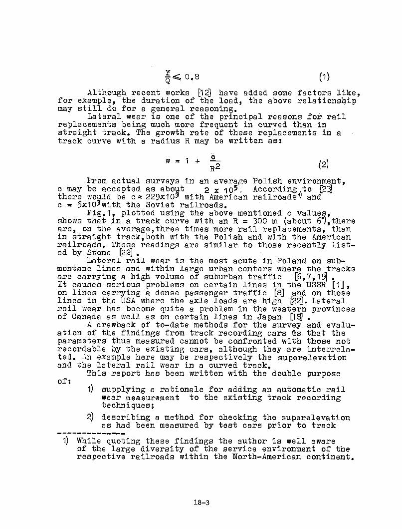
Although recent works [12] have added some factors like, for example, the duration of the load, the above relationship may still do for a general reasoning.

Lateral wear is one of the principal reasons for rail replacements being much more frequent in curved than in straight track. The growth rate of these replacements in a track curve with a radius R may be written as;

W a 1 + -2-R2

Prom actual surveys in an average Polish environment, c may be accepted as about 2 x 1 0 . According to [23] there would be c« 229.X10* with American railroads*) and c « 5-XIO^with the Soviet railroads.

Pig.1, plotted using the above mentioned c values, shows that in a track curve with an R = 300 m (about 6°),there are, on the average,three times more rail replacements, than in straight track,both with the Polish and with the American railroads. These readings are similar to those recently listed by Stone [22] .

Lateral rail wear is the most acute in Poland on submontane lines and within large urban centers where the tracks are carrying a high volume of suburban traffic [6,7,19] .It causes serious problems on certain lines in the USSR [1 , on lines carrying a dense passenger traffic [8] and on those lines in the USA where the axle loads are high [22]. Lateral rail wear has become quite a problem in the western provinces of Canada as well as on certain lines in Japan [18] .

A drawback of to-date methods for the survey and evaluation of the findings from track recording cars is that the parameters thus measured cannot be confronted with those not recordable by the existing cars, although they are interrelated. An example here may be respectively the superelevation and the lateral rail wear in a curved track.

This report has been written with the double purposeofj

1; supplying a rationale for adding an automatic rail wear measurement to the existing track recording techniques;

2) describing a method for checking the superelevation as had been measured by test cars prior to track

1) While quoting these findings the author is well aware of the large diversity of the service environment of the respective railroads within the North-American continent.

f « 0 . 8 ( 1 )

18-3

5 «

F ig . 2 . The param eters determining lateral rail w ear

18-4

18-5

Fig.3. Measurement of lateral rail wear using a vernier gauge.

f " , , *i '• '

Fig.4. Measurement of rail wear using a profilograph of the MR Yoshida Seiki type.A local spot of wear may be noticed behind the profilograph.

maintenance, that is at a time when - in order to reducelateral rail wear - the superelevation may yet be modifiedwithout a surplus expenditure in workload and manpower.

2. Lateral rail wear measuring techniquesLateral rail wear may be described by two parameters:1) an e dimension corresponding to the loss of material

at a determined level of the rail head /usually 15 mm below the running surface/;

2) the rail cant angle <P /Fig, 2/.There is a feeling among Polish specialists that a consi

deration of the worn area alone may be suitable for a comparative study of various rail types, but much less in diagnostics, which is meant to serve chiefly prac^ical purposes.

The procedures known so far for the measurement of lateral rail wear may be roughly classified into two categories:

1. Those only supplying the e dimension and leavingthe wear profile undetermined. Various types of vernier gauges are in use to this effect /Pig.3/;

2. Those informing on the cross-profile of the worn rail,i.e. various types of profilographs /Pig.4/.

With a profilograph, then, the rail s cant angle may be determined. The disadvantage of this procedure is its being extremely slow.Besides, neither of them would be reliable in the case of a local or irregular lateral rail wear in curved or straight track /Pig.5/. To reproduce such a wear with a profilograph, the measurements would have to be spaced every 1 - 1.5 meter, which is only possible on short test track sections. It would be unrealistic to recommend this procedure for track diagnostics, basically implying a continuous recording over the whole length of a line.To counteract the track deterioration processes, or - at least - to be able to reduce them, their origin, their scope and the dynamics of their growth must be known. This also includes lateral rail wear. Wanting to evaluate the effectiveness of any means for their prevention, the wear should be measured automatically.The easiest to automatize would be the measurement of the linear dimension alone, without determining the V angle.What will be said hereafter in Chapter 3, shows that it is quite possible to thus confine the measurement.

The lateral rail wear could be measured using a microwave technique in the 10 GHz band. An overall schematic of such a system is represented in Pig.6. Noteworthy here is the oblique position of the waveguide convergence transformer permitting the rail wear to be measured in turnouts or in grade crossingsi.e. wherever there would be a check rail besides a normal one.

18-6

18-7

Fig.5. Non-uniform lateral wear vanishing beyond the joint.

Fig.6 .Schematic of the '—system for an automatic measurement of lateral rail wear:

1 - GUNN oscillator;2 - standing wave factor

meter,-3 - wave-guide;4 - wave-guide convergence

transformer;5 - sliding edge (horizontal

basis);6 - roller (vertical basis);7 - rail;8 - check rail.

This calls for the determination of a new dimension e5 instead of the previous e one.

3. Correlation between the depth of wear e and the rail cant angle

To determine this correlation, worn rails have been measured on a mass-scale [7] with a Yoshida Seiki profilograph, type MR /Pig.4/. The results were surveyed and processed separately for two populations, covering respectively:

1) tracks operated in intercity passenger and in freight service, both electric and diesel hauled,

2) tracks operated in suburban electric trainset service.The relationship achieved for the first population was

<P= - 0.71 e + 78.95 [ ° J (3)with a correlation coefficient r = - 0.649.

Por the second population the relationship was- 0.17e + 66.80 [ °] (4)

with a correlation coefficient r = - 0.254.The correlation was confirmed by t - Student test to be

significant in both cases.A survey of the findings from lateral rail wear mesure-

ments revealed the following:(1) electric trainsets operated in suburban service tend

toward wearing the upper fillet of the railhead more severely than the intercity vehicles. Even with a wear of 1 - 3 mm the Wangle was then by about 15°/0.262 rad/ smaller than in the case of a new railhead.

(2) No case of lateral wear was recorded in either population, when the ? angle would be smaller than 60°/1.047 rad/. This also refers to such cases when thee value had exceeded 20 mm. It should be noticed that a minimal wear angle has been accepted at 55° in both German Republics, at 60° in Prance and at 64° in Great Britain.

(3) The considerably lower correlation coefficient achieved for the tracks operated in commuter service may be explained by a greater irregularity of their alinement. It may be proved by a comparison of the versine variation index equal to:- Vf = 48.7 % on intercity lines- Vf » 72.4 % on suburban lines.

Considering that no angles sharper than 60° , i.e. angles capable of imperilling the safety of traffic were found as a result of the measurements, it would be possible to confine the automatic recording of lateral rail wear for diagnostic

18-8

purposes to the sole measurement of the linear wear, i.e. that of e or es ,The measurements with a profilograph could be therefore confined to research purposes.4. A survey of curved track superelevations over

the whole length of a line, with due account taken of rail wear.

The measurement of lateral rail wear, be it effected with the existing techniques which are very simple or with the anticipated, more sophisticated ones, are still aimed ats

1. Determining whether the worn rails may still be left in the track or will have to be replaced.This calls i.a. for a scientific determination of the permissible wear limit. Investigations carried out by the PKP have shown that this limit couldbe raised from 10 to 20 mm [7] .

2. Supplying the necessary data for an analysis of the effectiveness of the procedures intended to reduce lateral rail wear.

Several procedures are known to this effect, as for example the lubrication of rails, the installation of a check rail /a third rail/, the use of harder steels, a better lining and surfacing of curves etc. But there is one among them, which so far has been somewhat underrated, namely the adjustment of superelevation within some feasible limits. The merit of this procedure is that it may be used together with any other, and - as already said - does not require any additional manpower expenditure, since it may be effected during track renewal.

The advantages of this procedure have been appreciated by the PKP upon a survey of the superelevations in 2600 track curves. In a large part of them the superelevation had to be modified [3] .

However, a mass-scale check of superelevation over whole railroad lines, including the rail wear, calls for the development of a method which, would be at once quick,accurate and generally accessible.

The author has wanted it to be a heuristic method, programmed for a calculator, so that the hardware would be inexpensive but would meet all the necessary requirements in most of the engineering calculations connected with railroad

1) By the way, the author has already designed several algorithms for track geometry optimation as a software for a TI-59 calculator.

18-9

It has been assumed, for this method, that a well-fitted, superelevation should meet five limiting requirements;

(1) The maximal unbalanced acceleration amox when passenger trains are running at their maximal speed Vp, must not exceed the acceptable acceleration value a<i1'2

amax = ~R s ^ ad (5)whereR - curve radius, h - the existing superelevation, s - the distance separating the center lines of

both rails.With the unbalanced acceleration known as well

as the parameters of a determined locomotive - the load of the Y force upon the rail may be calculated.A relevant computing method has been developed and put into actual practice by Erskov [11] .It results from his studies [10] that the acceleration a and the force Y are linearly interrelated /Pig.7/. The effect of a deficiency of superelevation on the value of the Y force has also been recently examined by Weiss [25] .

The tests of several dozens of various prototype vehicles (cars and locomotives) carried out by our Institute for nearly twenty years, have pointed out that the lateral Y forces are strongly affected by the vehicle design and by the quality of track maintenance. A heterogeneous track would account for a very differentiated dynamic force input, even over a short track length [5] . The deformations due to quasi-statical loads would also be variegated [26] . As shown by Prause and Kish [21] the dynamic forces will give greater standard deviations on curved than on straight track. All this shows the advantage of regarding as approximate the analytical relationships between the Y forces and the accelerations.

The permissible acceleration ad is accepted in Poland at 0.6 m/sec2, which corresponds to deficiency of cant equal to 90 mm. It is then lower than the deficiency accepted with the American railroads [9] at 4-5" /102-127 mm/.pAn ad = 0.6 m/s has beenaccepted chiefly to prevent an excessive value of the Y forces.

i) This refers to a theoretical acceleration value, not the actually measured one, always exceeding the theoretical [3.4] .

18-10

18-11

YlkNJ

F ig .7. Y forces as a function of unbalanced acceleration a according to [10] 1 - electric locomotive 6 s 200; R “ 1000 m,2 - ditto , except R * 2000 m ,3 - electric trainset ER200; R*2000m

(2)

When adequately designed, passenger cars may run smoothly even at an a<i = 1.0 m/s2 [20] . This lies beyond the unbalanced acceleration limit accepted in the USA for ride comfort considerations at 0.08 g [1 6] .The maximal unbalanced acceleration an in freight trains running at a speed v* , should not exceed at. An overloading of the inside rail is pre-supposed when a, has a positive sign.

v.n

hs (6)

The higher the annual traffic load qp [10 tons/year] carried by a line, the lower should be the permissible at value. This relationship has been represented in Pig.8 as accepted with the Polish /PKP/, the Prench /SHOP/ and the West-German /DB/ railroads.

(3) The wheel-climb speed f should not exceed a permissible value ffl

a v n hf = 3?6 1 ^ fd (7)

where1 - length of superelevation ramp.Henceforward a term m = 3.6 fd will be introduced

in the calculations referring to the relationship (7).Accepted for fd are values ranging between 22 and

47 mm/s, with a prevalence of 27.8 mm/s, due to the common use of the following equation for the length of the transition curve.

1 v h m

v hToTT (8)

On a rugged terrain 34.7 mm/s are commonly accepted, as indicated by equation

1 v hT 2 5

(9)

When well-founded, the transition curves may be yet shorter.

(4) The existing superelevation h should be at least, equal to a hp value, below which there would be problems with maintenance operations, but is not to exceed hg. The limiting value hg has been dictated,i.a. by a fear that the carried goods might be displaced in the cars, that the clearances might be exceeded etc.

h p«£h=shg (10)

The validation of (10) requires no calculations and will not be included into the algorithm.- In Poland,the accepted levels are hp * 10 mm and hg =* 150 mm.

18-12

18-13

at [m/s2]

0.9

0.8

0.7

0.6 _______ JU

0.5

0.4

0.3

0.2

0.1

SNCF, jvt = 120 km /h\ ,SNCF, v,

SNCF (exceptional ly)

= 100 km /h (exceptionally)

„SNCF, v ,=100km /h :

I DB. fvp $ 160 km /h*_

> M a — . ft m

sac?

PKP

D B .vp >160 km /h !( liiii _______ - .

ii•

at or PKPQr

flO^on/year* t

0 < q < 5 0 .65 < q < 1 0 0 .5

1 0 < q c1 5 0 .41 5 < q < 2 0 0 .3

q > 2 0 0 .2

__________

- - - - - -

10 15 20 25 30 qr [10®ton/year]

F ig .6 . Acceptable acceleration values a , as a function of annual tra fic load q

The general block diagram of checking superelevation is given in Pig.9. Similarly to the detailed one, shown next, it was designed as a software for the calculator. It is a procedure the best suited for checking the superelevation over the total length of a line, usually including several dozens if not several hundreds of curves. It grants a speedy calculation with a simultaneous analysis of several variants when the superelevation does not meet certain limiting requirements.

The first step following i he input of data is an overall check-up of the superelevation’s meeting all the requirements /variant A/. If so, it should be additionally verified, whether there are or no any special comments referring to the investigated curve, namely was there any excessive lateral rail wear?

In the presence of such remarks, the upper and lower limit should be determined for the superelevation /variant C/.

With a strong wear of the inner rail, or with the steel- plates deeply cut into the ties supporting the outer rail, the superelevation should be increased up to a value close to the calculated upper limit. With far reaching crushings and protrusions found in the inner rail, whereas the outer rail has been hardly worn, the existing superelevation should be reduced.

If, in variant A, the existing superelevation were found not to meet any of the limiting requirements, then the actual acceleration values and wheel-climb speed will have to be checked /variant B/. Should these values but insensibly exceed the permissible ones and the wear would not be strikingly higher with one of the rails - then the existing superelevation might be left unchanged.

That would rather mean a formal modification of the initial requirements. Otherwise, variant B should be followed by variant C and by a modification of the actually existing superelevation.

The algorithm has been block-diagrammed in detail in Big.10. Having entered the values of the parameters envisaged for the surveyed track curve, i.e. R,l,h, the A key would be depressed to answer the question whether all the requirements are met by the superelevation, or whether one or more of them would not. In the first case,the figure 102 would appear on the disjJay. In the second,there would be displayed a flashing 505 \ Variant B overlaps on part of the blocks belonging to variant A /blocks 2,3,4/ and ends upon a display of the values

a max» a n ar1^

1) Use was made of a mnemotechnical rule: In colloquialPolish "102" means "O.K.", while "505" on the display may also be read as "SOS", i.e. as an alert.

18-14

© ©

©( e n d * )

Validate: amax < ad , an ^ at , 3 .6 f < m ;

Calculate: amax , an , f (subsequent to A cycle) ;

Calculate: hmin, , h „ ^ .

F ig . 9 . General block diagram for checking the superelevation of curved track

18-16

V 2a - p -0.0065h-m ax 12.96 R

3 *

an =0.0065h v«J12 .9 6 R

(START)

EnterVariant A and B: R1vp)vt ,ad1at l l,m,h Variant C : R , I tv vt , ad , at , m

I I " ' '

11.8vp2»W =

12 ♦u(D -.m l-.."max'" Vp

13 _____ ! _____... 11.8v2

h ^> = R +153a,

Fig. 10. Detailed block diagram for checking the superelevation of curved track

Variant C covers the calculation of hmin, h o* , h dx (hmin being followed by the display of one only of the two values calculated for hmaj(, the lesser one). It may easily be noticed that hftL is a function of the permissible wheel-climb speed f, and h ^ - a function of the permissible unbalanced acceleration at.

The equations in the detailed block diagram are converted relationships (5) , (6) and (7) , the train speed being written in kmph, the superelevation in mm, the acceleration in m/sec2 and the wheel-climb speed over the superelevation ramp - in mm/sec.hi s = 1500 mm and a g = 9.81 m/sec2 were ■ accepted.

The check of superelevation after the above algorithm was programmed as a software for a TI-59 calculator.

Integrated into the program is an example of superelevation check in four curves. In curve 1 no amendment is required for the superelevation. In curve 2 it was decided to slightly reduce the superelevation although it had met all the requirements. The reason was an excessive wear /flattening out/ observed in the inner rail. In curve 3? the pre-determined fj value was not achieved despite a reduction in the superelevation and it was decided to abandon the requirement, hoping that this modification would anyhow improve the position.An alternative, here, was a reduction of the train speed. Lastly, in curve 4, an amendment was made permitting all the requirements to be met.

5. ConclusionsLateral rail wear being a serious problem with many Rail

roads, an automation of its measurement should become one of the priority tasks in the field of track recording. This measurement may be confined to one linear parameter thus permitting the use of a microwave technique.

One of the ways of reducing the lateral wear of the rails is an adequate adjustment of the superelevation to suit the service environment on the line concerned.

The procedure described hereabove for the checking of superelevation in curved track allows a rapid determination of the amendments to make during a continuous track renewal.The amendments may also be made at the moment of a routine track maintenance.

The work content of such calculations seems negligible against their effect in the shape of even a slightest gain in the service life of a track.When an automatic measurement of lateral rail wear would have finally become a current practice, a sub-system for an automatic amendment of superelevation might be included into the system processing the findings from the measurements of track geometry.

18-17

References1. Andrievskij S.N.: Bokovoj iznos relsov na krivych.

/Lateral rail wear in track curves/ Trudy CNII, No.207, Moskva 1961,p.5-128.

2. Baluch H.: Method of the optimum design of the crossing arrangement. Rail International 1970, No.8 ,p.601-612

3. Baluch H.: Wyznaczanie przechylki z uwzgl§dnieniem pr§d- kosci pocig,gow towarowych.. /Calculation of superelevation with a consideration given to freight train speed/.Przeglq,d Kolejowy Drogowy, 1976, No.3 P.1-9.

4. Baluch H.: Diagnostyka nawierzchni kolejowej./Diagnostics of railway track/, WKiL, Warsaw, 1978, 456 p.

5. Baluch H.: Assessment of a possible reduction in the number of test trips when measuring stress in the rails.Archiwum Inzynierii L^dowej, 1980, No.1,p.181-200.

6. Baluch H.: Trwalosc i niezawodnosc eksploatacyjna nawierzchni kolejowe3./Durability and service reliability of railway track/ WKiL0 Warsaw, 1980, 186 p.

7. Baluch Maria: Analiza kryteriow dopuszczalnego bocznego zuzycia szyn. /An analysis of the criteria of acceptable lateral rail wear/. Drogi Kolejowe, 1978, No.10,p.290-294.

8 . Cihak F.J.: A Theme for Rail Transit in the'SO-s... Make it Run. Progressive Railroading, 1980,No.8 ,p.33-36.

9. Doyle, Jr.G.R., Thomet M.A.: Effect of Track Geometry and Rail Vehicle Suspension on Passenger Comfort in Curves and Transitions. Journal of Engineering for Industry,1977, Nov.p.841-848.

10. Erskov O.P., Karcev V.J.: Teoreticeskie i eksperimentalnye issledovanija osobennostej dvizenija ekipazej so skorostia- mi do 200 km/h i trebovanija k soderzaniju puti./Theoretical and experimental investigations into the particularities of vehicle motion at up to 200 km/h and the requirements for track maintenance/ Zeleznye Dorogi Mira, 19 8 0, No.1,p.3-13.

11. Erlkov O.P., Zak M.0.: Kak vpisyvaetsa teplovoz CME3 w krutye krivye. /Hqw the Diesel locomotive CME3 takes sharp curves/ Put i Putevoe Chozajstvo, 1980, No.7,p.42-44.

12. Ikemori M., Sugiyama T.: Improvement of Running Safety of Freight Car. Quarterly Reports, Railway Technical Research Institute, 1978, No. 2. p.4-9 - 57.

13. Jakubowicz J.: Elektroniczny miernik wspolczynnika spokoj- nosci biegu pocig,gu "Wz" /Electronic Wz ride meter/ Automatyka Kolejowa, 1979, No.7-8,p.222-226.

18-18

14. Kishimoto S.: High-Speed Track Measuring Car. Quarterly- Reports Railway Technical Research Institute, 1979* Ho.4, p.145-152.

15. Klein R.s Railroad Research... Where Are We How? Where Are We Going? Progressive Railroading, 1980, Ho.6, p.31-34.

16. Kunieda M. s Several Problems about Rolling Stock Which Can Run on Curves at High Speed. Quarterly Reports,Railway Technical Research Institute, vol. 13, 1972, Ho.1, p.1-7.

17. Kupczyk Irena.: Elektroniczny miernik logarytmicznego dekrementu tlumienia drgari podkladow kolejowych. /Electronic decremeter for the measurement of cross-tie vibration damping/ Pomiary, Automatyka i Kontrola, 1979* Ho.1,P. 6-7.

18. Kurihava R.: Present State and Future of Railway Rails. Quarterly Reports, Railway Technical Research Institute, 1979, Ho.3, p.97-105.

19. Malejki E.: Zuzycie boczne szyn w lukach o malych promie- niach./Lateral rail wear in sharp curves/, Drogi Kolejowe, 1978, Ho.10, p.288-289.

20. Pandolfo A.: Eksploatacija novych infrastruktur z tocki zrenija obediniennych transportnych sistem. /Operating new facilities from the viewpoint of integrated transportation systems/, £eleznye Dorogi Mira, 1980, Ho.4,p.44-60.

21. Prause R.H., Kish A.: Statistical description of service loads for concrete cross-tie track. "Transp. Res.Rec.", 1978, Ho.694,P.30-39.

22. Stone D.H.: Comparison of Rail Behavior with 125-ton and100-ton cars. Bulletin AREA, 678, 1980, June-July,p.576- 587. ,

23. Sulga V.J.: Vychod relsov i spal iz stroja v krivych ucastkach puti i mery po jego snizeniju. /Rail and tie replacements in curved track and steps to be taken for the reduction of their scope/, Trudy MIIT, Moskva 1977,No. 556, p. 72-81.

24. -: Vlijanije Verchnego strojenija puti na povysenije skorostej dvizenija gruzovych poezdov. /Effect of the track on the increase of freight train speeds/, Zeleznyj Transport za Rubezem, 1974, Ho.1,p.38-45.

25. Weiss J.: Premises and conditions for High Speed Traffic from the viewpoint of the DB Permanent Way Service Transport International. Special Edition of "Internationales Verkehrswesen", 1979, October, p.74-80.

26. Zarembski A.M.,Mc Connel,Lovelace W.S.: Hew Car for Measurement and Evaluation of Gage-Widening Resistance of Track. Bulletin 678,AREA,1980,June-July, p.402-429.

18-19

T.i - 5 9

S u b m i s s i o n A b s t r a c t

Program T i t l e

C h e c k i n g t he s u p e r e l e v a t i o n i n c u r v e d t r a c k

L e v .

A b s t r a c t o f P r o g r a m:

The pr ogram p e r m i t s :

1 / to c he c k w h e t h e r t he s u p e r e l e v a t i o n i s k e e p i n g w i t h i n a l l

the r e q u i r e d l i m i t i n g v a l u e s , i . e . w h e t h e r t h e r e i s no

e x c e e d e n c e o f 1 / t he a c c e p t a b l e u n b a l a n c e d a c c e l e r a t i o n s

a^ and a t and 2 / t he a c c e p t a b l e v e l o c i t y o f w h e e l

c l i m b i n g on t he s u p e r e l e v a t i o n ramp f

2 / to c a l c u l a t e the a c t u a l v a l u e s o fdop

{ MA M( Mma x '

v a r i a n t ) ;

and f ( " B " v a r i ant)

3 / to c a l c u l a t e t he m i n i ma l and t h e ma xi ma l s u p e r e l e v a t i o n( 2 )(1)v a l u e h . , hmin max h %c~' ( "C " va r i a n t ) .max, '

I f v a r i a n t A has y i e l d e d a p o s i t i v e r e s u l t , no f u r t h e r

c a l c u l a t i o n s a r e r e q u i r e d . V/ith a n e g a t i v e outcome o f

v a r i a n t A , t he c a l c u l a t i o n s h a v e t o be p u r s u e d t o v a r i a n t s

0 and C , on t he gr o u nd o f w h i c h e i t h e r t he e x i s t i n g

s u p e r e l e v a t i o n or - w h e n e v e r j u s t i f i e d - t he o r i g i n a l

l i m i t i n g v a l u e s woul d be m q d i f i e d .

Program b y : Henry k B a l u c h , Wa r s z a wa

Us e r B e n e f i t s :

A q u i c k c h e c k and a d j u s t m e n t o f s u p e r e l e v a t i o n over

the t o t a l l e n g t h o f a r a i l r o a d l i n e .

C a t e g o r y Name: P r o g . S t e p s : C a r d S i d e s P C - 1 0 0 A Needed Cl

D i a g n o s t i c s o f L i b r a r y

t r a c k g e o me t r y!

2 5 0 2 Modul e . . . . n

18- 2Q

TI-59User I n s t r u c t i o n s

S t e p Pr o c e d u r e En t e r P r e s s O u t p u t /Mode

1 E n t e r program

2 E n t e r r a d i u s o f c u r v e R a '

3 E n t e r p a s s e n g e r t r a i n speed V p d '

4 E n t e r f r e i g h t t r a i n s peed v t c'5 E n t e r p e r m i s s i b l e a c c e l e r a t i o n a d D *

6 E n t e r a c c e l e r a t i o n f o r f r e i g h t t r a i n s a t E*

7 E n t e r l e n g t h o f t r a n s i t i o n c u r v e 1 D

8 E n t e r wheel c l i m b i n g speed l i m i t m STO 0 7

9 E n t e r e x i s t i n g s u p e r e l e v a t i o n h E

V a r i a n t " A"

. i.) Check wh e t h e r s u p e r e l e v a t i o n keeps w i t h i n a l l l i m i t i n g v a l u e s A

1 0 2 - y e s or

(505)) - no

V a r i a n t " B ”

onl y to f o l l o w V a r i a n t " A ”

1 1 Determi ne a c t u a l a c c e l e r a t i o n f o r p a s s e n g e r t r a i n s B a max

1 2 Determi ne a c t u a l a c c e l e r a t i o n f o r f r e i g h t t r a n s R/ S a n

1 3 Det ermi ne a c t u a l wheel - c l i mb speed R / S f

V a r i a n t “ C" I

1 4 C a l c u l a t e mi ni mal s u p e r e l e v a t i o n C ^m in

1 51

C a l c u l a t e maximal s u p e r e l e v a t i o n R/ Su)

( 1 1 ' h. a x(2)

^ ' hmax

18-21

T I - 5 9

Sample Problem

For a submontane l i n e with the f o l l o w i n g pa r a me t e r s :2

v = 80 km/h a . = 0 . 6 0 m/sP d m = 100

v = 60 km/h a f = 0 . 4 0 m/s

check s u p e r e l e v a t i o n in c urves whose c h a r a c t e r i s t i c s are as

f o l l o w s :

CurveNo

------7 T "R [m] 1 [m] h jmm] Remarks

1 1 0 3 0 1 3 0 65 -•

2 800 85 95 E x c e s s i v e wear of i nne r r a i l

3 350 70 140 -

4 4 7 5 65 1 2 5 -

Enter Press Output/Mode Comment

80 B# •o00 Entered VP

= 80 km/h

60 o ' 60. Entered v t = 60 km/h

.6 D' 0 . 6 Entered a d = 0 . 6 0 m/s2

.4 e ' 0 . 4 Entered a t2

= 0 . 4 0 m/s

100 ST0 07 1 0 0 . Entered m = 1 00

1030 A# 1 0 3 0 . Entered R1 = 1 0 3 0 m

1 3 0 D 1 3 0 . Entered = 1 3 0 m

65 E 6 5 . Entered h l = 65 mm

A 1 02 Curve 1 - O.K.

800 A ' 8 00 . «

85 D 8 5 . .Entered dat a f o r curve 295 E 9 5 .

18-22

;.n t er Press Output/Mode Comment

A 102 Curve 2 O.K b u t , t her e being some s p e c i a l remarks, v a r i a n t "C" has to be c a r r i e d o u t .

C 3 . h . = 3 mm min

R/S 1 1 0 6 . = 1 06 mmmax

D e c i s i o n : reduce h e s t i m a t i v e l y to 7 0 mm

70 A ' 70 Entered new s u p e r e l e v a t i o n

A 102 Confi rmed: p o s s i b i l i t y of mo d i f i c a t i o n

B 0 . 1 62

a „ „ = 0 . 1 6 m/s at h = 70 mm max '

R/S 0 . 1 12

a = 0 . 1 1 m/s at h = 70 mm n

R/S 1 8 . f = 1 8 mm/s a t h = 70 mm350 A ' 3 5 0 .

70 D 7 0 . ■ Entered data f o r curve 3140 E 1 4 0 . J

A ((505)) S u p e r e l e v a t i o n in curve 3 does not meet requi rements

CLR 0 Removed f l a s hB 0 . 5 0 = 0 . 5 0 m/s2 max '

R/S 0 . 1 2 a n = 0 . 1 2 m/s2R/S 4 4 . f = 4 0 mm/s > 2 7 , 8 mm/s

C 1 2 4 . h . = 1 2 4 mm m in

R/S

1

00 00 •

. 1hmax= 88 mm

D e c i s i o n : reduce h to 1 2 5 mm and abandon f ^ s 2 7 , 8 mm/s

1 2 5 E 1 2 5 . Entered new s u p e r e l e v a t i o n h = 1 2 5 mm

A ((505)) Repeated checki ngCLR CLR Removed f l a s h

' B 0 . 6 0 amax= 0 , 6 0 m/ s 2 at h = 1 2 5 mm

R/S 0 . 0 2 a^ = 0 . 0 2 m/s2 at h = 1 2 5 mm

R/S 4 0 . f = 4 0 mm/s at h = 1 2 5 mm47 5 A ' 4 7 5 .

65 D 6 5 . ■ •Entered data f o r curve 41 2 5 E 1 2 5 .

A ((505)) S u p e r e l e v a t i o n in curve 4 does not meet requi rements

CLR 0 Removed f l a s h

18-23

E n t e r Pre s s Output/Mode

B

R/S

R/S

C

0 . 2 3

0 . 2 3

4 3

67

a max

a n

f

h . mm

Comment

0 . 2 3 m/s2

0 . 2 3 m/s2

4 3 mm/s >

6 7 mm

2 7 , 8 mm/s

80

R/S ( l ) , 8 1

E 8 0 .

A 102

(1J8 1max

D e c i s i o n :

Conf i r me d

mm

r e du c e h t o 80 mm

p o s s i b i l i t y o f m o d i f i c a t i o n

B

R/S

R/S

0 . 5 2

- 0 . 0 6

2 7

a = 0 . 5 2 m/s2max ' 2a = - 0 . 0 6 m/sn

f = 2 7 mm/s

A l l r e q u i r e me n t s met

Codes s

(n) s h o r t d i s p l a y (ca 0 . 5 s e c )

((n)) f l a s h

1 8 - 2 4

Program title:

Checking the superelevation in curved track

TI-59 Program

LOC KEY LOC KEY LOC KEY LOC KEY LOC KEY

OOO LBL 052 02 104 X S T 156 2 208 X

001 k * 053 X 2 105 RCL 157 RCL 209 RCL002 STO 054 106 04 158 12 210 03003 01 055 RCL 107 GE 159 R/S 211 X 2004 R/S 056 16 108 CLR 160 RCL 212005 LBL 057 109 LBL 161 13 213 RCL006 BV 058 RCL 110 CE 162 R/S 214 01007 STO 059 01 ill 2 163 FIX 215 +008 02 060 — 112 5 164 0 216 1009 R/S 061 RCL 113 5 165 RCL 217 5010 LBL 062 17 114 0 166 14 218 3Oil ( T 063 X 115 2 167 RTN 219 X

012 STO 064 RCL 116 5 168 LBL 220 RCL013 03 065 08 117 + / - 169 C 221 05014 n / s 066 = 118 VX 170 FIX 222 =015 LBL 067 STO 119 R/S 171 0 223 STO016 D' 068 12 120 LBL 172 1 224 11017 STO 069 RCL 121 CLR 173 1 225 RCL018 04 070 17 122 RCL 174 • 226 10019 R/S 071 X 123 13 175 8 227 X3-T020 LBL 072 RCL 124 X $ T 176 STO 228 RCL021 e ' 073 08 125 RCL 177 15 229 11022 STO 074 — 126 05 178 X 230 INV,023 05 075 RCL 127 GE 179 RCL 231 GE024 R/S 076 03 128 X 2 180 02 232 i/X025 LBL 077 X 2 129 GTO 181 X 2 233 RCL026 D 078 130 CE 182 -T 234 09027 STO 079 RCL 131 LBL 183 RCL 235 R/S028 06 080 16 132 X2 184 01 236 1029 R/S 081 -r 133 RCL 185 - 237 PAU030 LBL 082 RCL 134 14 186 1 238 RCL031 E 083 01 135 X 187 5 239 10032 s r o 0S4 S 136 3 188 3 240 RTN033 o s 085 STO 137 • 189 X 241 LBL034 R/S 086 13 138 6 190 RCL 242 1/X035 LBL 0S7 RCL 139 = 191 04 243 RCL036 A 088 02 140 I 4 T 192 — 244 09037 i 089 X 141 RCL 193 s r o 245 R/S038 2 090 RCL 142 07 194 09 246 2 •039 • 091 08 143 GE 195 RCL 247 PAU040 9 092 -r 144 V X 196 07 248 RCL041 6 093 3 145 GIO 197 X 249 11042 STO 094 • 146 CE 198 RCL 250 RTN043 16 095 6 147 LBL 199 06044 • 096 • 148 V T 200 -r045 0 097 RCL 149 1 201 RCL046 0 098 06 150 0 202 02047 6 099 St 151 2 203 s048 5 100 STO 152 R/S 204 STO049 STO 101 14 153 LBL 205 10050 17 102 RCL 154 B 206 RCL051 RCL 103 12 1 55 FIX 207 15

18-25

D I S C U S S I O N

Mr. Dyer; Have you done any analysis with the microwave technique you pointed out?

Mr. Baluch; As yet, no. In spite of the microwave technique, we consider also a technique in the megahertz band because, as you know, the maximum dimension of the measurement, linear measurement, may be here one of force of the bands. That means 7.5 to 8 mm. only, and therefore, there is the possibility first, to adjustment points between the head of rail and the measurement equipment or second, to analyze a correlation between the dimension "a" and the smaller dimension on the upper part of the railhead.

Mr. Lovette (Southern Railway): In Poland, have you made any correlationbetween railhead profile and derailment?

Mr. Baluch: It is difficult to say that there is a correlation, because I understand that I can say about correlation if I can present a coefficient of correlation, let us see, 0.6, 0.7, and so on. In, this mathematical sense, we haven't any correlation. But there are many observations that in such places, in such sections of track, in which the angle is below 60 , derailments are very often, especially such cars as cement cars.

Mr. Lovette: Would you say that again, the 60° statement.Mr. Baluch: If the angle of the declination of the flange is smaller

than 60°.Mr. Kumar (IIT): Maybe I can translate that. The slope of either the

wheel surface or the rail surface can decide whether there will be a climb.The angle that is usually considered critical has been the flange angle for the derailments, and what we are hearing here is that if the rail angle is also becoming very small, then this becomes the controlling critical parameter.We found the same thing in our experiments, by the way. Sixty degrees is an angle that we also found to be a critical one.

Mr. Baluch: Practically, there are two limits - 60 and 55. This isdangerous already if there is 55.Mr. Brantmen: Russ Brantman, TSC. Has any work been done on developing

an optimum cant angle as a function of superelevation?Mr. Baluch: No. It is quite independent.

1 8 - 2 6

REQUIREMENTS AND TECHNIQUES FOR MEASURING DYNAMIC DISPLACEMENTS OF RAILROAD TRACK COMPONENTS

Donald R. Ahlbeck Franics E. Dean

BATTELLEColumbus Laboratories

505 King Avenue Columbus, Ohio 43201

Measurements of the displacements of rails and ties have traditionally been used to investigate vehicle-track dynamic interactions. Before the development of wheel/rail load transducers, measurements of dynamic displacements of track components provided an estimation of the load environment under passing rail vehicles. Now, in conjunction with the measured wheel/rail and track component loads and strains, dynamic displacements provide an invaluable measure of track strength and mechanical characteristics. In this paper, the basic requirements of displacement measurement transducers, fixtures and instrumentation are reviewed. Currently-used techniques for measuring both absolute and relative displacements in both wood tie and concrete tie track are described. Recent experiments in which displacement measurements have played an important role, including the Perturbed Track Tests at the Transportation Test Center and rail fastener performance evaluation tests on the FAST track, are cited as examples of current displacement measurement technology.

HISTORICAL BACKGROUNDMeasurements of the displacements of rails and ties have traditionally been used to investigate vehicle-track dynamic interactions. Before the development of sophisticated load cells and strain gage patterns to measure the rail-to-tie loads and wheel-to-rail loads, deflections of the track structure were utilized as a "poor man's" load transducer. Unlike the wheel/rail load measurements, on which a substantial body of literature exists, little has been published on the requirements and techniques for measuring dynamic displacements of track structural components from the wayside.Early measurements of track vertical deflections were static or quasi-static in nature. The AREA^ utilized a 66-inch (1.68 m) beam to measure the deflections of a rail joint under vertical load. Other experimenters have used optical methods, such as viewing a millimeter scale attached to the rail through a surveyor's transit, to determine deflections under slowly-moving wheel loads. Dynamic deflection measurements have also been made. Birmann2 makes casual mention of "buried probes" in the measurement of track depressions under locomotives at speeds up to 124 mi/h (200 km/h) on the German

19-1

Federal Railways (DB). Nield and Goodwin of British Rail (BR) report the use of vertical displacement potentiometers in their study of dynamic loading at rail joints .Development of differential transformers during the 1950’s provided the needed tool for dynamic displacement measurements . This type of transducer was utilized by Battelle for track deflection measurements on the Chessie System and on the Penn Central Northeast Corridor track in 1969 and 1971 > . These measurement techniques were considerably refined in an investigation of the wide gage phenomena on tangent high-speed track? conducted under the auspices of the Track Train Dynamics Program. Studies of the dynamic response of concrete tie track under revenue traffic have also used deflection measurements to investigate fastener load environment and to establish track modulus values. Displacement measurements during the recent Perturbed Track Tests at the Transportation Test Center near Pueblo, Cororado, have proven invaluable in establishing track strength limits under dynamic vertical and lateralloading9jlO.

TRACK DEFLECTIONSTrack deflection measurements include absolute deflections of the rail relative to a fixed reference, and relative deflections between track components. These deflections may occur in all six degrees of motion freedom: vertical,lateral (transverse) and longitudinal translation; and angular motions of rail in roll (in the transverse plane), pitch (longitudinal rocking), or yaw of the rail. Vertical and lateral translation and rail roll angle are of primary interest. The longitudinal motion, known as rail "running", is seldom measured dynamically, although it is a direct measure of a rail fastener/ anchor's ability to restrain the rail longitudinally. On wood tie track, this motion can exceed an inch with a reversal of traffic direction on poorly- anchored rail. Yaw motions of the rail are considered of little consequence except, perhaps, under buckling conditions.Several absolute and relative displacements are needed to describe fully the upper track structural response to dynamic loads. These are:(1) Rail vertical absolute displacement— used to define the track modulus and

dynamic load/deflection characteristics.(2) Rail head/tie lateral displacement— used to measure rail lateral

restraint characteristics under both lateral and vertical loading.(3) Tie/ground lateral displacement— data under revenue traffic can document

the infrequent occurrence of lateral shift of the tie in the ballast; used to establish track lateral strength limits.

(4) Rail rotation (roll)— used to document the mode of rail deflection and loading on tie/fastener system.

(5) Rail rotation (pitch)— used to determine loading environment on tie/ fastener system.

(6) Rail/tie vertical displacement— used to determine dynamic load/deflection characteristics and loading environment on tie/fastener system.

19-2

(7) Rail longitudinal displacement— used to determine tie/fastener rail restraint capabilities.Two primary difficulties encountered when making dynamic deflection measurements are survival of the transducers in the rugged environment and establishing references from which the measurements are to be made. Establishing "absolute" reference points adjacent to the track structure requires going deep enough, or far enough to the side of the track, to locate ground which does not move relative to the track. While pressures in the ballast/subgrade drop off quickly to something less than 3 lb/in (21 kPa) at a depth of 40 inches (102 cm), both track structure modeling and field experiments have shown vertical deflections to decrease with depth more slowly. At a 40-inch depth, typically half the vertical deflection will still be measured.Past experience has shown that absolute deflection measurements related to rail joint or rail fastener performance can be referenced to "ground" by attaching the transducer to a rod driven down into the subgrade. In the concrete tie track studyS, a 1-inch diameter steel rod was driven through a concentric hollow pipe casing through the ballast into the subgrade. The casing was about 4-ft long to isolate the rod from ballast movements; while the steel rod was 8 ft long and was driven into the ballast/subgrade until only about 8 inches projected above the ballast surface. In other field experiments, shorter rods have been used driven directly through ballast into the subgrade without benefit of the casing. Vertical deflections using a 4-ft rod showed a range from 0.10 to 0.14 inch under locomotive axles, while static calibration (viewed through an off-track transit) showed 0.18 inch deflection under a 30,000 lb (133 kN) point load.Relative measurements must also be isolated from undesirable displacements.For example, if dynamic track gage is to be measured and the tie is used as a reference for individual rail displacements, then tie bending could readily distort the intended output. The deflection fixture developed by Battelle for the Track Train Dynamics Program? is an example of a measurement system that provides dynamic displacement measurements of the rail without distortion from bending of a wood tie. A conceptual drawing of this fixture is shown in Figure 1, and Figure 2 shows the relative displacements which are measured. In addition, the fixture provides some degree of shock and vibration isolation for the transducers and signal conditioning electronics through elastomeric grommets and lag screws mounting the fixture to the tie. Acceleration levels on the tie can range typically up to 50 g under flat wheel impact loads. Typical deflection measurements from the fixture shown in Figure 1 are illustrated in Figure 3. Dynamic track gage and rail rollover (of one rail only) under severe lateral impact loads due to empty freight car, truck hunting are seen here, along with about 1 mm of permanent lateral shift of the tie.In measurements on much stiffer concrete ties, a fixture which eliminates the effects of tie bending was found unnecessary. A conceptual drawing of a fixture used for recent measurements of concrete tie fastener/pad deflectionsl3 is shown in Figure 4. Here the measured rail-to-tie displacements, along with fastener clip strains, were used to define the loading environment of rail fastener systems. Data were collected on both wood and concrete tie track segments containing a variety of fastener systems, and the results were reproduced in the laboratory to determine the required level of loading which

19-4

FIGURE 1. STABLE BASE FIXTURE FOR UPPER TRACK STRUCTURE DYNAMIC RESPONSE MEASUREMENTS UNDER WHEEL/RAIL LOADS

FIGURE 2. MEASUREMENTS OF RELATIVE AND ABSOLUTE DISPLACEMENT NEEDED TO DEFINE UPPER TRACK STRUCTURE DYNAMIC RESPONSE TO WHEEL/RAIL LOADS

19-5

W heel detecto r pulse

llll 1111 HU llll III! 1111 till llll 1111 1111 1111 llll< f f i m m m m ' r r o i o i o f o O U. U. u. Li_ o O <J o < - >UJ -1 —1 _1 _1 _l _l UJ kJ Ui UJ UJ

-»-■

40

.00

0

(178

kN

)

T ie plote ve rtic a l load

A K K A K A L , ^ ^ ^

0-4

In.

—

(1

0 m

m)

Dynam ic gage Increase

T im e — ►

R a il ro llo v e r O ut1«r> •

Si

_ i ____

0.2

In.

—

9-

(5 m

m)

T ie absolute la te ra l m otion

0.2

In.

(5

mm

)

Down^ R a il-a b s o lu te v e rt ic a l m otion

ATW A\AN\f\r\jv\FIGURE 3. TYPICAL TRACK DYNAMIC RESPONSE MEASURED FROM TRACK TRAIN

DYNAMICS PROGRAM INVESTIGATION OF WIDE GAGE ON HIGH-SPEED TANGENT TRACK — REVENUE FREIGHT TRAIN AT 62 MI/H

19-6

19-7

FIGURE 4. FIXTURE FOR MOUNTING RAIL/TIE DISPLACEMENT TRANSDUCERS

In an application of the fixture shown in Figure 4, typical deflections for concrete and wood tie curved track are illustrated in Figures 5 and 6. M e a surements were made with both deflection transducers and strain gaged fastener clips. In these time histories of deflection under loaded FAST train cars, differences in "signature" between concrete tie track (Figure 5) and wood tie track (Figure 6) can be seen. On the concrete tie track, a combination curve and grade, the rail rolled outward and the gage clip received substantial uplift strain. The wood tie track was fastened with the same elastic clip attached to a steel tie-plate. Very little clip strain developed, but the vertical rail/tie deflection was greater because the tie plate experienced bending as it conformed to the nonuniform surface of the wood tie.

DISPLACEMENT TRANSDUCERS

s im u l a t e d f i e l d c o n d i t i o n s . T h e l o a d l e v e l s s o d e f i n e d w e r e t h e n a p p l i e d i nf a t i g u e t e s t s o f t h e f a s t e n e r s y s t e m s .

A variety of displacement transducers are suitable for making track deflection measurements. The optimum transducer type and range may vary, depending on the specific application. Criteria that must be considered in the choice of transducers arell»12;

(1) Transducer range— track structural deflections may range from less than 0.25 inch (6.4 mm) to greater than 1 inch, full range (vertical deflections under load of 1-3/4 inches, 44.5 mm, have been observed at weak rail joints). Typical expected deflection ranges are:

Vertical, absolute Vertical, rail/tie Lateral, rail head Lateral, rail base Longitudinal

Concrete or wood tie track,

positive fasteners, good condition

0.25 in (6.4 mm) 0.15 in (3.8 mm) 0.25 in (6.4 mm) 0.10 in (2.5 mm) 0.10 in (2.5 mm)

Wood tie track, cut spikes,

good condition

0.50 in (12.7 mm) 0.25 in (6.4 mm) 0.75 in (19.1 mm) 0.40 in (10.2 mm)

**

Wood tie track, poor condition

1.0 in (25.4 mm)* ** 0.5 in (12.7 mm) 1.5 in (38.1 mm) 0.5 in (12.7 mm)

**

* Greater deflections at joints in poor condition.** Rail may "run" under traffic...must be checked at site.

(2) Transducer accuracy— resolution, linearity and hysteresis commensurate with measurement goals must be achieved.

(3) Frequency response— a transducer bandwidth of 100 Hz is usually sufficient for deflection measurements. Deflections decrease rapidly with increased frequency (remember, even a 500 g oscillation when at 700 Hz is only 10 mi ls ).

(4) Instrumentation compatibility— power requirements, output voltage level and impedance, good signal/noise ratio, etc.

(5) Ruggedness— vibration tolerance and shock survival g levels suitable to transducer mounting point.

19-8

FIGURE 5. TYPICAL RAIL/TIE DISPLACEMENTS AND FASTENER CLIP STRAINS ON CONCRETE TIE TRACK — LOW RAIL ON 5-DEGREE CURVE

19-9

.1"Compfitulon VERTICAL FIELD 0 LEFT

CompA.fc4AionVERTICAL F IELD 0 RIGHT

11 se^. j

r ~ \ / ~ \ r * \ f ~ \ / ~ \ f ~ \

.rCom pA.zA 4i.on

VERTICAL GAGE 0 LEFT

^ ^ y^\ y-\ y~\

O utua A dRAILHEADLATERAL

p \ . / - \ y \

.0 5 "Ou&ocAdRAILBASELATERAL

0 r\ n n r\~7h.0 5 "

FIELD o LONG. [w — ^ ^

1 0 0 0p i n / i n

UpliftGAGECLIP

IUUUp i n / i n

UpU£tFIELDc l i p

_____________ ______________________________________ _________ ___________

FIGURE 6. TYPICAL RAIL/TIE DISPLACEMENTS AND FASTENER CLIP STRAINS ON WOOD TIE TRACK — HIGH RAIL ON 5-DEGREE CURVE

19-10

(6) Electrical noise immunity--not affected by stray electrical signals in rail due to signalling or power return.

(7) Electrical isolation from rail— cannot ground rail signals.

(8) Insensitivity to other motion degrees of freedom— primarily a function of the transducer mounting fixture design and transducer attachment scheme.

(9) Ease of calibration in situ— transducer must allow system end-to-end physical calibration under field conditons.

(10) Protection from environment— the transducer should preferably by hermetically sealed against moisture, salt spray, dust, sand, etc.

(11) Transducer cost.

Although the displacement transducer in itself does not affect the track characteristics, it is usually difficult (as discussed in the previous section) to establish an ideal point of reference from which the deflection measurements can be made. Optical tracking systems have been used in the past, without great success, to measure rail vertical absolute motions at a point well away from the track. Ground vibrations have introduced noise into these measurements, or target lighting has caused problems. An Australian firm has recently introduced a laser tracking system with the detector head mounted to the rail and a tripod-mounted low-power laser set typically 16 ft (5 m) away from the track. A range of +10 mm (0.4 inch) and a frequency response of 0 to 1 kHz is noted in the technical specifications.

Displacement transducers have accuracies that are typically better than necessary for this particular application, as long as the full-scale range of the transducer is well-matched to the actual displacements. However, care must be taken to insure that sufficient frequency bandwidth is available to monitor the frequencies of interest. Noncontacting displacement transducers (the eddy current type) have more than sufficient bandwidth, but must be calibrated during installation to correct for target geometry and material properties. Some electrical noise problems have been encountered in the past in use of these transducers with electrified (power-return) rail on the 25-Hz Northeast Corridor line.

Contacting transducers utilize either direct attachment techniques or spring- loaded plungers. It is difficult to provide sufficient spring preload and stiffness to prevent contact separation in the frequency range of interest without at the same time causing some flexure of the reference fixture.Direct fixation of the core of differential transformers through nonmagnetic threaded "ready rod" to a phenolic block cemented to the rail has proven quite successful in the past. The cemented block is able to withstand the high rail acceleration levels (shock pulses over 1000 g have been recorded under flat wheels) and provide electrical isolation from the rail. The rod also provides sufficient isolation from orthogonal motions of the rail, particularly- the rail "running" motion in the longitudinal direction, yet is reasonably immune to its own transverse vibrations. This arrangement is susceptible to ice, ballast, or dragging equipment, and for more permanent installations a protective shroud is recommended.

19-11

D i f f e r e n t i a l T r a n s fo r m e r

Past experience has shown that the Linear Variable Differential Transformer (LVDT) offers excellent performance characteristics for measuring dynamic displacements. The LVDT consists of a primary transformer winding excited by a sinusoidal voltage of 3 to 15 volts rms amplitude, and a frequency from 60 to 20,000 Hz. Two series-opposing secondary windings have sinusoidal voltages induced in them by the primary. As the iron core of the transducer is moved relative to the secondary windings, a larger mutual inductance (coupling) is induced in one relative to the other, and a net voltage increase is produced from the device. The output voltage undergoes a 180° phase shift when going through the null (zero) position^. A fully-integrated version of the LVDT, called the DCDT, has built-in high-frequency excitation and signal conditioning, providing the demodulated direct-current signal at the output. This transducer provides a DC signal directly proportional to the relative displacement of the core to the transducer body. Output voltage levels range up to +20 volts full scale for an excitation up to 30 volts DC (older models required both the plus and minus voltage polarities). Typical DCDT specifications range as follows:

Working Range*Frequency Response

(-3 dB) Linearity Ripple

0.050"0.10 to 0.25" 0.50 to 2.00" 3.0 to 10"

300 to 500 Hz 115 to 500 Hz 100 to 110 Hz 50 to 75 Hz

0.25% to 0.5%0.5% of to 1%full of fullscale scale

* 30% to 50% overrange is typical.

These transducers are extremely rugged, with typical mechanical specifications allowing a vibration tolerance of 10 g to 2 kHz, and a survival shock level of 250 g for 11 milliseconds pulse duration. Therefore the transducer can operate satisfactorily in the shock and vibration environment typical of the railroad tie, but cannot be mounted directly to the rail.

In field applications, Battelle has powered the DCDTs directly from the signal conditioning amplifiers, which provide the 5 volts DC excitation and (depending on the specific model of DCDT) output levels from 1 to 3 volts full scale. Some additional attenuation before recording is occasionally required.

Calibration

One important aspect of transducer choice is the ease of physical calibration under field conditions. In this respect, the DCDT is probably the most straight-forward transducer of any to use. Aluminum body clamps with a slightly greater internal diameter than the DCDT body diameter, and split along one face, are used to hold the DCDT. These are loosened slightly so that the body of the DCDT can be moved relative to the fixed core with slight finger pressure. The null (electrical zero) position is first established, and then the body is moved through a given distance, using a machinist's scale to measure the clamp-to-body displacement. The resulting voltage is then read at the signal conditioning amplifier, and the voltage amplitude adjusted as

1 9 -1 2

necessary. An end-to-end calibration is desirable, and therefore the null position, mid-range position, and full-scale position are generally recorded on tape, on the oscillograph or strip chart, and on the digital data output system. After calibration, the DCDT body is clamped in its original position. Occasionally this rest position is offset from the electrical zero to allow greater transducer stroke in one direction versus the other.

REFERENCES

(1) AREA Special Committee on Stresses in Track, 5th Progress Report, Proceedings of the AREA, Vol. 31, pp. 75-336, 1930.

(2) F. Birmann, "Track Parameters, Static and Dynamic", Inst. Mech. En gr s, Proceedings 1965-66, Vol. 180, Part 3F, pp. 73-119.

(3) B. J. Nield and W. H. Goodwin, "Dynamic Loading at Rail Joints",Railway Gazette, Aug. 15, 1969, pp. 616-619.

(4) E. 0. Doebelin, Measurement Systems, McGraw-Hill, 1966, pp. 233-242.

(5) H. C. Meacham, et al, "Studies for Rail Vehicle Track Structures",Report No. FRA-RT-71-45, April 1970.

(6) D. R. Ahlbeck, C. W. Rodman, and H. C. Meacham, "Collection and Analysis of Data on Penn Central High-Speed Track Response at Bowie, Maryland", Battelle Summary Report to DOT/FRA, Oct. 27, 1971.

(7) D. R. Ahlbeck, H. D. Harrison and S. L. Noble, "An Investigation of Factors Contributing to Wide Gage on TAngent Railroad Track", Journal of Engineering for Industry, Vol. 99, Series B, No. 1, Feb. 1977, pp. 1-9.

(8) R. H. Prause, et al, "An Analytical and Experimental Evaluation of Concrete Cross Tie and Fastener Loads", Report No. FRA/ORD-77/71, Dec. 1977.

(9) H. D. Harrison and J. M. Tuten, "Perturbed Track Test Program Wayside Measurements", Battelle Interim Report to DOT/TSC, Aug. 1979.

(10) M. Coltman, R. Brantman, and P. Tong, "A Description of the Tests Conducted and Data Obtained During the Perturbed Track Test", Report No. FRA/ORD-80/15, Jan. 1980.

(11) R. H. Prause and H. D. Harrison, "Data Analysis and Instrumentation Requirements for Evaluating Rail Joints and Rail Fasteners in Urban Track", Report No. UMTA-MA-06-0025-75-8, Feb. 1975.

(12) D. R. Ahlbeck, et al, "Evaluation of Analytical and Experimental Methodologies for the Characterization of Wheel/Rail Loads", Report No. FRA-OR&D-76-276, Nov. 1976.

(13) F. E. Dean, "Research Plan for the Development of Improved Rail Fastener Performance Requirements", prepared by Battelle's Columbus Laboratories for the Office of Rail Safety Research, Federal Railroad Administration, Contract DOT-FR-9162, April 1980.

1 9 -1 3

DISCUSSION

Mr. Brantman: Russ Brantman from TSC. Could you go into a little moredepth on the problems you had with the eddy car transducers? Exactly what were some of the problems?

Mr. Ahlbeck: I'm really digging back in the memories. This was in 1976,and we didn'.t really make a concerted effort on checking the thing out. You know, it's the usual case where it's a fire drill in one of these test programs, and you say, "I'm going to test this transducer" and you hook it up and everything and then just before you're going to tear it down, you say, "Oh, I never got anything out of that." But we did get some O-graph traces on passing revenue trains and, as I remember, we saw rather high noise from the 25 Hz. and harmonics. And also, by just moving it in and out, we found that there was considerable non-linearity in the output voltage versus distance.

Mr. Caldwell: Nelson Caldwell, CN Rail. Don, you showed a slide of - Ithink you called it, an optical scan camera - that had been used previously.Is that one of these optical line scanning cameras on a diode array?

Mr. Ahlbeck: It's called an optron, it has a black-white target on therail head and it senses and it probably has several internal, and it tries to minimize on that transition line.

Mr. Caldwell; What's wrong with them, or what difficulty did you encounter with them?

Mr. Ahlbeck; Well, this was not our experiment and it was just hearsay that they were getting a considerable amount of noise from ground vibrations as the train passed and they were also having lighting problems that, when the train came by, it shadowed the target and you got a sudden change in gain.

Mr. Hickock; Dick Hickock, Wyle Labs. I had experience with that optron unit when I was at the Test Center. You can solve the light-dark transmission by putting a lit target on the rail. It had the shadowing effect and changed the beam of light to a flicker.

Mr. Caldwell: Aside from that light problem does it do the job?

Mr. Hickock: Oh, yes. W e got quite a bit of usage out of it. Once yougot the position target, it worked quite well.

Mr. Caldwell: How far can you be? What sort of lenses would you use?

Mr. Hickok; (Inaudible)

Mr. Ahlbeck: We got some recent literature about two months ago froman Australian company that is marketing a laser displacement transducer which apparently does use an array. They use a laser light and then an array. But I guess the laser light is mounted on the rail and the array is back in the transducer.

1 9 - 1 4

M r . Palmer: Doug Palmer, Arthur D. Little. At the perturbed track tests,we were lucky enough to have a panel shift, but we weren't lucky enough to have displacement transducers nearby. Is there a development in technology or mass production or something that can give us or increase the possibility of instrumenting a long section of track?

Mr. Ahlbeck: You know, there are some cheap and dirty transducers, Iwould call them, they are sort of friction type things. They use them for gauge, to measure maximum gauge. However, we found out that they shorted the rail out, too, in the rain and we upset AMTRAK. But anyway, these things are fairly inexpensive. I think ENSCO has a batch of those. They've used those and you mount them and then come back at some time later and the indicator will show by friction where the maximum position was.

M r . Yang (ENSCO): The cost involved there is reading them and resettingthem. You have to have people to walk through the whole area.

Mr. Ahlbeck: Right. You really don't know what it was that did this,unless you stay there and watch.

Mr. Merrill: Dave Merrill, Thomas K. Dyer. Don, you showed a curve onthe dynamic displacement in regard to unit vehicle weights, gross weights.Would you run by that again? You did it rather quickly and I didn't quite get it. Just explain.

Mr. Ahlbeck: Okay. The vertical axis is normal probability scale andthe horizontal axis was dynamic gauge which, as I said, is somewhat proportional to lateral load. So what we have there are probability curves of the occurrence of high dynamic gauge or high lateral load, and it showed three curves there. One was for light cars, and that showed the greatest amplitude at a given level of probability. The heavy cars showed the lowest amplitude.

1 9 - 1 5 / 1 9 - 1 6

SESSION 4: PROBLEMS, OPPORTUNITIES, FUTURE NEEDS AND TRENDS

INTERNATIONAL CONFERENCE ON WHEEL RAIL LOAD AND DISPLACEMENT MEASUREMENT

TECHNIQUES

SESSION 4: PROBLEMS, OPPORTUNITIES, FUTURE NEEDS, TRENDS

Chairman: S.C. Chu

Office of University Research


January 20, 1981

TABLE OF CONTENTS

INTRODUCTION BY MR. CHU

PANEL DISCUSSION I

Presentation by Mr. Tsai

Presentation by Mr. Spencer

Presentation by Mr. Smith

PANEL DISCUSSION II

Presentation by Mr. Pocklington

Presentation by Mr. Anderson

Presentation by Mr. Baluch

Presentation by Mr. Zuck

Presentation by Mr. Xu

DISCUSSION - GENERAL

CLOSING REMARKS

INTRODUCTION BY MR. CHU

MR. CHU: The Fourth Session of this conference is devoted to a discussion of

problems, opportunities, future research needs and trends. My name is

Sherwood Chu. I'm the Director of the Office of University Research at the

DOT from Washington.

20-1

The Office of University Research sponsors a research program which is

dedicated to universities. Our office is not a mission office in the sense of

the FRA or the Urban Mass Transportation Administration. What our program

does is to determine priority research needs on a department-wide basis, and

then we put out a solicitation annually to the universities in a variety of

problem areas and solicit their proposals.

We have an interesting program set up for you this afternoon. It will feature

a couple of Panels. The first one will feature representatives from the U.S.

DOT and a representative from the National Research Council of Canada. The

DOT representatives are the able session chairmen from yesterday, Tom Tsai and

Paul Spencer, and our representative from Canada is Cam Smith, who is the

section head of the railway lab at the National Research Council of Canada.

The first speaker this afternoon will be Tom Tsai of the FRA.

PRESENTATION BY MR. TSAI

MR. TSAI: Mr. Chairman, the title of the session is Problems, Opportunities,

Future Needs and Trends. I will try to address this subject within the next

five to ten minutes. But first, on behalf of the FRA, I would like to thank

Dr. Pin Tong and the TSC staff for the fantastic job they have done during the

last two days. The conference is very successful, and I believe all of you

feel the same way. We have learned something here in the last two days. I

hope we can take it home with us.

The Problem, as we have identified it, involves force, displacement and other

measurements. As far as we are concerned, FRA will continue to support this

area of research, because we have many programs that require this kind of

measurement and we need the data not only for research, but also for

regulatory purposes. In this regard, I think there are long-term and short

term needs. For the long term, FRA is committed to the development of TTC,

the Transportation Test Center. Over there, we have the Rail Dynamics

Laboratory and many testing tracks, which need advanced measurement techniques

as well as modeling and supporting capabilities. Therefore, we are committed

to developing better and broader systems. For the short term, our particular

areas of interest are illustrated by some slides that I have here to show you.

Figure 1 shows one of the trucks we tested last year. We have evaluated

20-2

several advanced freight and passenger car trucks over the past few years.

Every truck design required different measurement techniques. The measurement

devices and the analysis techniques have to be modified for each design.

Therefore, we had to develop not only systems for the current equipment, but

also systems for advanced equipment being developed for the railroads.

Figure 2 shows the angle-of-attack measurement device used by Canadian Pacific

Railroad. It is a laser device. I think that, in the future, advanced

systems using laser and other optical devices will be frequently used to

measure the performance of advanced equipments being developed. Figure 3

shows the angle-of-attack system developed by Wyle Laboratories for TDOP,

using a non-contact eddy current device. Figure 4 shows another design,

developed by ENSCO, using a similar principle. Although we encountered many

problems in developing these systems, we did accomplish some good

measurements. These figures represent some of the recent advances in angle-of-

attack measurement systems. I believe that we still need continuing research

in this area before we can understand the important phenomenon of wheel/rail

interface. As we are all aware, the analysis of the wear of the rail and the

wheel, as well as the vehicle dynamics, depends on our knowledge of the

wheel/rail interface. As a result of our recent studies, we now have better

methods in measuring the wheel/rail forces. Hence, we should now develop a

more reliable angle-of-attack measurement system to go with the force

measurement systems.

Finally, I want Ito say a few words about the trend of our research. As I can

see from this conference, the trend is toward more cooperation not only

between the Government and industry, but also between the United States and

other countries. In the past, one could work by himself in his own small

corner. Today, we are all working together. Furthermore, there is increasing

cooperation today between the analysts and the testing engineers. The diverse

attendees at this conference demonstrate that cooperation indeed is real in

research on wheel/rail interface.

20-3

Figure 2. CP Angle-of-Attack Measurement System

20-4

Figure 3. Wyle Angle-of-Attack Measurement System

Figure 4. Ensco Angle-of-Attack Measurement System

20-5

PRESENTATION BY MR. SPENCER

MR. SPENCER: I am here from the Urban Mass Transportation Administration.

That agency is represented by the mode shown on the left and the mode shown on

the center of your program guide. The particular office which I represent,

the Office of Rail and Construction Technology, focuses upon the middle mode

entirely, namely conventional urban rail transit.

Although wheel/rail interaction has been of interest to that office throughout

the test programs, the early programs at the Transportation Test Center at

Pueblo, Colorado and the Major Vehicle and Subsystem Development Programs that

we have conducted, it is only within the last two years that the subject of

wheel/rail dynamics has been given the status of a separate program. Since

our former R&D office has for the last few years been called the Office of

Technology Development and Deployment, we perform both of those activities in

wheel/rail dynamics. That is, we perform both generic technology development

and provide direct assistance to transit authorities on specific technology

related problems. We have been trying to strike what Professor Sweet referred

to yesterday as the proper balance between research and problem solving.

Although I must confess that it's not a fifty-fifty balance in our office, it

is very heavily slanted nowadays toward problem solving.

We rely very heavily on T S C ’s technical and managerial expertise to assist us

in these areas. Examples of site specific problems currently underway include

the following: investigation of axle bending stresses on the MBTA; study of

direct fixation, rail fastener failures on the WMATA; evaluation of the Budd

Company radial axle trucks on the Port Authority Transit Corporation, PATCO;

design of the UTDC, Urban Transit Development Corporation radial axle truck

concept for the Washington Metropolitan Area Transit Authority; wheel rail

wear investigation on the Port Authority Trans Hudson, PATH, system.

The generic studies underway are devoted to various specific aspects of the

problem, such as truck performance studies, performance surveys, wear index

studies and verification, probably to get under way next fiscal year, various

wear studies and various parametric analyses in areas such as wheel rail

forces and displacements. The UMTA program interacts with transit

authorities, both directly and through the American Public Transit

20-6

Association, APTA, for which we are in the process of sponsoring a separate

APTA Advisory Board in wheel rail interaction. This Board will consist of

representatives from each of the North American Rail Transit properties.

Our program is also interrelated and co-ordinated informally with the FRA and

with other UMTA sponsored research programs, in particular, the Ways and

Structures program recently completed at the Transportation Test Center.

Other Pueblo testing is the current dynamic testing of the state of the art

car in the rail dynamics lab which is to get underway in the next week or two.

And finally, the Urban Rail Noise Abatement which is, although

programmatically separate and distinct from wheel rail interaction, of course,

technically they are very closely related.

We in UMTA are very fortunate in not having to start from scratch in this

area. We have an existing technology base upon which to draw. This knowledge

base was built largely by contractors for the Federal Railroad Administration,

the Association of American Railroads, and international sources such as those

represented at this conference. Thank you.

MR. CHU: Are there any questions for Paul with respect to the UMTA program.

Would you please identify yourself?

MR. CALDWELL: Caldwell from CN Rail Research. I was interested to hear your

comments that one of the programs y o u ’re monitoring is rail wear in transit

systems. I'm wondering if maybe you could comment on it for a freight

railroader. Is it similar to the wear we're seeing in freight systems? What

kind of wear and mechanisms are involved?

MR. SPENCER: No. I'm sure the mechanism has a lot in common with the

mechanism from a physics and engineering point of view with rail wear on curve

problems where they arise. We do have a larger percentage of our system in

the form of curves and the curves are substantially sharper. The study that

we recently completed was done in Washington. Is that the one that you're

specifically referring to and you want me to address?

MR. CALDWELL: Yes.

20-7

MR. SPENCER: Washington Metro was experiencing wear rates probably an order

of magnitude faster than they had expected in certain locations such as the

approach to Washington National Airport. We, on very short notice, assembled

a team consisting of TSC engineers, Battelle Columbus Labs, and ENSCO.

They came in during off-revenue service, took the measurements. These were

parametric studies. Some of the parameters looked at were tapered versus

conical wheels, acceleration from a start in the curve, velocity through the

curve, lubricated versus unlubricated, slight gage variation. We found that

some of these parameters which we had suspected would be sensitive turned out

to be insensitive, such as the velocity and acceleration. Some of them seemed

to be key, such as the taper of the wheel. We found that we could reduce

lateral forces under some conditions as much as one-third by adjusting a

parameter such as wheel taper. These conclusions were passed on to the

Washington management, and they are, as far as I know, taki ng.action on them.

MR. KUMAR: I am Sud Kumar from Illinois Institute of Technology. The subject

of wheel rail interaction and wear has been of considerable interest to us.

In addition to what has already been said by Mr. Spencer, the plasticity

effects, as is obvious perhaps, are considerably different between the transit

systems and the freight systems simply because of the contact stress range.

In the case of freight systems, you will get maximum theoretical contact

stresses of up to 250 KSI, whereas for the transit systems, these would be of

the order of a hundred and some KSI which is still acceptable for the rail

type high carbon steels that we have under combined stress situations.

The other things, of course, are the profile effects and the conicity, as well

as the possible cant differences. I found in one study that the angles of

attack in transit systems can be very, very much higher simply because they

have often sharp curves to negotiate, whereas in the trackage for the

traditional freight service or traditional intercity service, those types of

sharp curvatures are either not acceptable or generally not designed. I

suppose metallurgy in terms of the wheels, of course, are known to be slightly

different in terms of hardnesses, and that makes an additional difference.

One other difference that I find which is creating a serious problem in some

systems, is that in transit systems, such as Bay Area rapid transit or even in

20-8

the Washington area, the grades that have been necessary to design are

considerably higher than would be the grades in a freight system. Design

addition values, particularly in BART, were around .18, and when you have an

addition quotient of .18, you can continue to operate except that many times

under oil and diesel or oil and lubrication which may be a contaminant on the

track, you do n’t achieve that and creates certain additional problems. The

requirements of curving combined with high adhesion make it also even more

complicated for the transit systems. So even though the contact stresses are

considerably lower, the additional problems make it much more demanding in

many cases.

MR. HARRISON: (Battelle Columbus) I might add a couple of other things that

are along the same lines in terms of general observations, having been

involved in the WMATA job. Again, there are parametric differences that

somewhat contrast the normal freight conditions. Number one, the vehicle

design or system design as a whole, I think is rather typical, that somehow

top speed stability tends to be the overriding criteria on the parametric

decisions on the design of the vehicle. Typically what you end up with are

longer wheel base trucks, stiffer suspensions, and in this case, the primary

suspension of the vehicle was a rubber donut type system around the wheel

bearings, and when they aged or settled, they got stiffer, and when you

combine those conditions, and then turn around and induce them into the

curvatures. The one we tested on down near the airport was around 700 or 750.

You combine all those things and you end up with probably much larger slip

conditions or moire creep conditions than would normally be found. Again, in

spite of the fact that the loads are down, the amount of net wear that's going

on is up and the net result is still a lot of rail wear.

MR. CALDWELL: Typically, what is the percentage of route that might be curved

track in a transit system?

MR. SPENCER: I don't know.

MR. CALDWELL: Over 50 percent?

20-9

MR. KUMAR: It depends how you define it. If you define it above 1 degree,

then that's a lot of track.

MR. CALDWELL: On our Main Line Railway, one of our worst curvature areas, (a

680-mile route) 37 percent of it is in curved track.

MR. YANG: Ta-Lun Yang from ENSCO. Just one more comment on this wear problem

between the transit and railroad. On most transit properties in this country

or other, countries, restraining rail is very commonly used in sharp curves,

which serves to guide the train by contacting the back side of the wheel on

the low rail side. Now this, in some cases, shares the wear and in other

cases, takes all the wear. Lubricating the restraining rail reduces the wear.

You usually couldn't do that on the high rail because of the possibility of

too much grease getting at the running track, so that's one of the ways that a

transit system reduced the wear problem.

MR. TSAI: Another side comment. One difference between transit and freight

rail is the noise. Whenever you get high wear in the transit, you get a lot

of noise like Larry Sweet mentioned yesterday. That's another transit problem

associated with the wear.

MR. TONG: Maybe I should comment on the restraining rail. If you really want

to reduce wear then the best design may not be a restraining rail to pull the

rail back. I think if you look more from an engineering or technical point of

view based on fundamental mechanics principles, there should be a better way

to attack the problem for sharp curves.

MR. RIESSBERGER: I can't give another observation but if you look to the

angle of attack, I must say that I was very much impressed by the Suldana Line

in South Africa where they use these self-steering bogies or trucks. I don't

know whether there is a program in the states which looks after this design.

The problem came in when they used the heavy locomotives, brand new

locomotives with the rigid truck, and then the wear started on the curves

20-10

where they had no wear over two years now. Another thing is, and this is a

proposal, the angle of attack certainly depends on the curvature of the line

and on the free play between the wheelset and the track, and if you reduce

this free play that means to tighten the gauge, then you get also contact on

the rear axle of the bogie and this reduces the angle of attack. So this is

one of the things which should be able to reduce the angle of attack and

subsequently also reduce the wear.

MR. SPENCER: Let me address that, please. We became aware of this work that

you're referring to several years ago as well as the successful demonstration

of steerable trucks on both the Canadian National and the Canadian Pacific in

Freight application. To date, there hasn't been a successful application in

conventional transit and the closest thing to it was the Intermediate Capacity

Transit System vehicle, the ICTS vehicle developed by UTDC in Kingston,

Ontario. That, of course, did have a linear induction motor propulsion system

and didn't involve throwing a heavy rotating mass on top of the mechanism, and

we feel that there is great hope for steerable trucks in transit applications

in the United States. In fact, that's why we undertook not one, but two,

parallel efforts to push development of the steerable truck. If it works, it

could be the most significant breakthrough in transit technology of the

decade, because it not only works favorably as far as wear is concerned, but

it also would virtually eliminate squeal noise in curves as well as conserving

energy, and it seems like this is one of those rare instances where all the

parameters work in a favorable direction. There are however, potential

stability problems, hunting problems on tangent track and the conditions of

very low friction, and certain conicity regimes, and we are aware of that, and

we are pursuing that optimistically.

MR. RIESSBERGER: I have nothing to do with the Scheffel bogie, but I feel the

same way you do, that it is one of the big steps which can be achieved. There

were excellent results also with steered bogies before the Second World War,

and then there was in Germany, I have to say, where the position of the

wheelsets was controlled by the movement of the body over the track. Also

this design has very small wear.

20-11

MR. TSAI: Let me add to what Paul said. In the slides I showed a while ago,

there was one slide that showed the truck which was a radial truck, and FRA

has conducted many testings on various radial trucks which include the design

by Scheffel and in fact, in the United States and Canada, we have many radial

trucks like that being put into revenue service. So we are aware of this and

we know that they are able to reduce the angle of attack. We are talking

about 10 minutes, 5 minutes, something very small. That's where we get the

problems, trying to define this quantitatively. As for locomotives, I have no

comment. I saw somebody's proposal saying that locomotives can use radial

axles. But for freight cars and transit cars, we do have ongoing projects to

take advantage of the radial truck. One problem is how to define cost

effectiveness. That's why we are investigating measurement techniques.

MR. RIESSBERGER: For the benefit of the audience, I want to say that I'm very

well aware also of the negative points of this bogie because if the contact

situation changes, say, in running over turnout, then this bogie starts to

move the axles. So in the turnouts there is a slightly different and

sometimes severe pattern of wear, but in the curves, it's much better.

MR. TSAI: That's true. We also worry about the turnouts. In addition, we

also try to test all the radial trucks in curvature up to 16 degrees of curve

(very sharp curve). We think it's a potential problem, it may or may not be.

We don't know yet.

MR. SPENCER: Let me say that we aren't pursuing the Scheffel truck out of any

prejudice toward that particular design concept. Rather, the initial intent

was a competitive award, and it was. For some reason or other, the Scheffel

truck wasn't part of that initial competition. They didn't respond to the

request for proposal.

MR. ANDERSON: Mr. Anderson from Swedish State Railway. We also have the

bogies in Sweden for iron ore transportation purposes, and we found that

putting in the primary rubber spring between the side frame and journal box

reduced the wear, flange wear, to about 50 percent. This is the action of the

creep forces which are then utilized to align the axles more regular in

curves.

20-12

MR. CHEN: My name is Chen from Washington Metro. I think it may be well to

be clear or clarify some points the gentlemen make here. We do have a rail

wear problem, but not systemwide. They are about 2 percent or so which means

they only mean 2 with a 1,000 feet radius on the curves, and the wear patterns

seem to be based on the testing information we had, as Paul mentioned before,

as located at the airport. In this particular location, we had a track with a

radius of about 800 foot radius, and we also have 4 percent grade, and it also

rests partially on ballast track and the other part rests on direct fixation

track. We had the most problems on the ballast track. And the operation of

the train is stopped at that point, every train go there five minutes or

whatever the schedule we have. So it means the oscillation of the train when

y o u ’re going uphill also contributes to this additional wear because we have

identical track on the other downhill side and we had no wear on the other

side. The train is just coming down the hill and goes the way it should be.

In the other areas, we do have some wear but it is not any worse than other

transit systems. We sent questionnaires to ask how they experience it, for

comparison. We do have wear, and essentially, it seems to be due to several

reasons. Our truck stiffness may be possible. We still don't know because

that's a part of our investigation and UMTA, Paul's office, is helping us.

And the other portion of wear is that perhaps we have some other geometry on

the track which means that we have unbalanced superelevation. In other words,

we do not use the superelevation in the tunnel. The idea was to cut down the

construction cost. Every foot of a higher tunnel increases many dollars. And

in addition, when you design superelevation, you only can design a certain

speed. Now, we Iknow pretty well some of the trains do not go to the curve at

exactly 40 miles per hour, and also we try to provide passenger comfort. In

the event the train stops on the curve, then the train will be inclined in

such a way that people feel like they're leaning on one side. So that's why

the superelevation is not going, say, six inches. We have four and a half

inches only. But we are also going to do a testing section. We are going to

either raise or lower the track, I believe we are going to lower the lower

track to provide a fully creep tie with superelevation to see whether we can

reduce the wear. In addition, we are going to update our restraining rail as

Dr. Yang mentioned. We are also trying to provide some lubrication and it

seems to be successful. By raising the superelevation plus the lubrication,

it seems to do the job. Lubrication is very messy and we found out that we

2 0 -1 3

have to be very careful because in the operation, we may have the signals and

automatic train control, we have disk brakes, so there a lot of things we had

to consider. We're going slowly doing our work, but I think the problem, at

least so far, has been identified. We're going to solve it slowly. Maybe a

year from now, we'll have something to tell you better, say, this is a

solution which may be better for other systems. Thank you.

MR. CHU: Our third speaker on this particular panel is Mr. C.A.M. Smith, of

the Railway Lab of the National Research Council of Canada.

PRESENTATION BY MR. SMITH

MR. SMITH: Thank you. Mr. Chairman and distinguished engineers, it's

certainly a great pleasure to be here and take part in your discussion.

However, I'd hate to do this under false colors. I work in a government lab,

it is true. However, I don't know that the things that I say would reflect

exactly how government agencies think in general because ours is a problem

solving laboratory largely, just as you mentioned, and the things we expect to

do will be largely, influenced by the questions we're asked and the jobs that

we're asked to do.

However, it's the time of year when we normally go through the throes of a

five-year plan, and so I have just been arguing the case of various funds for

new ideas, so I have a few ideas that you might find of interest. Just don't

assume that this is the view of the Canadian government, which it's probably

quite the reverse.

In arguing the case for these various funds, I came across several arguments.

Some are quite negative and should be fought with all one's might. For

example, they say there is a shortage of money and research and development

can be cut with no loss of service. As soon as the return to investment gets

up above the rate of inflation, we can rehire a great crew and do wonderful

things.

Also, they say the interchange rules define so many features of a car design

that any rapid change is ruled out. They also say that a significant number

of the 2 million cars on this continent must be altered before any real

2 0 -1 4

significant change occurs in their dynamic behavior. For example, Mr.

Caldwell’s radial trucks - h e ’s got 10 carsets or so in a fleet of a hundred

thousand, and the rails are still wearing out. There's no point. The time

lag imposed by these last two arguments will exceed the working life of

several engineers, you see, that are perhaps the spearheads of some of these

forward-looking things. And without the spearhead, the program will probably

flounder. But you must debate and refute these negative arguments with all

your might. In the face of a declining percentage of freight shipped by rail,

money must be found to solve the shipper's problems with this most energy

conservative method of land transportation.

Captive fleets are the place to start. You don't have to change the whole

system if you have parts of your fleets that are captive fleets. When the

ideas have proven'sound, they will spread like measles. An elite class of

service, for example, preferably in multi-mode service, plus efficient

terminals will be the thin edge of a wedge that will bring a lot of shippers

back to the railroad.

Cars carrying dangerous commodities should be specially equipped with methods

for monitoring temperature and pressure, security, vibration, noise, and

placed in a rather special or elite part of a train where they can be under

constant surveillance, because bad press is a thing we don't particularly need

much more of in the railway business.

The alternative, anyway, to these arguments is what happened to the dinosaur

when the climate changed. For the immediate future, what can we do? We much

improve our understanding of the wheel rail interface and y o u ’ve heard all I

guess you want to hear about that up to now. But we also must be able to

sense when a bearing is in distress, a sill is cracked, and where the roadbed

is undermined. We must devise facilities where the real world can be

simulated, where new ideas can be tried out in safety and security.

Now, for example, in our own laboratory, we have under construction a

full-sized variable curvature track simulator to look into curving behavior

and stability margins of novel trucks in the laboratory. This simulator has

been designed to reproduce as closely as possible the real world, the real

20-15

live track, including spin, creep, and many other features. It is taking a

long time. It'll take a bit more time, but it's the sort of thing we feel we

should be doing. We have assembled fatigue environment measuring equipment

and some heavy shaking equipment to enable car builders to know the vibration

environment and observe their car's response to this environment in the

laboratory. We are enlarging the capability of our climactic environment

chamber to accept a railway vehicle. This room replaces a facility, which,

among other things, was used to develop two entirely new types of ice-free

rail switches, and a number of improved brake system components. We have

commissioned a wear rig which you heard about this morning. Dr. Kalusek in

Vancouver, NRC, has a one-eighth scale wear rig that produced most of the

pictures you saw in the first paper this morning. We have been investigating

means of measuring angle of attack for over ten years, and have produced some.

In fact, we had a hand to play in the ones you've heard of from Dr. Ghonem

this morning. In fact, we've been working on one now that will leave the

space between the rail sacrosanct. If you've got a linear motor between the

rails, you can't very well use the laser method, and we've produced a very

satisfactory type of zero-crossing signal that we feel will allow us to turn

this to discovering angle of attack with fair accuracy.

For the longer term, we've been asking for funds and staff to develop

practical means for monitoring and performance of all the elements in a train,

including the roadbed. We feel the train crew has a serious handicap with no

modern aids to continually check on the system that has very rarely, but very

catastrophic accidents. And we have also asked to be allowed to study wheel

and brake interaction at low temperatures. That's another curious thing up

north. The brake system so happily used down here isn't always that marvelous

up north. Whether we get these funds or not, our lists for problems,

opportunities, future needs and trends are as follows.

In the problem line - slow reaction to improved competition, not an

engineering problem particularly, but it's still a problem with railroading,

particularly freight railroading. And, I think, for the other as well; poor

information to train crews on the condition of track, the train, the lading;

failures of components too often lead to disasters, unnecessary disasters

because of this. Poor vertical ride in freight cars due in part to the

2 0 -1 6

coupler height requirement. Poor longitudinal of long trains related to

slack, braking, and poor instrumentation. That's poor, I mean, in this day

and age. We're not talking about poor in 1880. It was great then. Next,

fatigue failures in high-mileage, heavy cars, excessive wear on curved track,

to both the wheels and the rails. For every dollar you waste on the wheels,

you waste ten on the rail.

Opportunities, second category - that was the problem category - I'm sticking

to the schedule. Opportunities in the nuclear age and with space age

electronics, we should be able to re-invest some of these fallouts of other

technologies into the railway business.

Firstly, low power and inexpensive instrumentation for surveillance of car

performance and safety, not so much research tools, but tools for the crew.

Readily available analysis equipment, for example, discovering the mechanical

impedance of the soil, the ballast, the bridge structure - the whole thing is

well within the means that we have at our disposal now. Continuous monitoring

by every train of the roadbed condition for the benefit of the road crew,

particularly with regard to potential disasters. More reliable signaling and

data handling with built-in redundancy. I've been on one of our Via trains

from Montreal to Ottawa, a distance of 100 miles. The train was two hours

late because the CTC - it rained that day, you see. Electrification of the

heavily used lines where the choice of nuclear, hydro, of fossil fuels is

there. At least, you can make a choice. Plus regeneration in hilly country

gives a permanent edge over highway traffic.

Future needs - better tools - this is a bit of reiteration, but nonetheless,

they are future needs and it's a future need that happens to have an

opportunity. Better tools for the train crews, the train inspectors, and the

track repair crew, particularly with regard to dangerous situations. Soil

mechanics should lead us to better measurement and compacting devices. Better

tools for the car designer - that's the purpose of this curved track simulator

I was speaking of earlier. Better protection from vandals and for grade

crossings. Axle loads commensurate with rail and wheel metallurgy and with

track structure.

2 0 -1 7

Now the trends - certainly the trends are to more radial trucks or steering

trucks, as we have been calling them. To multimode freight and away from the

boxcar. To multi-source energy. Again, to give the train crew more than two

levers, a pressure gauge, and an ammeter with which to control the train. We

will continue, that's we at the National Research Council, will certainly

continue our problem solving to help the Canadian railroads, the users, and

help them quantify such things as rail and wheel profiles, the ride, the wear,

the forces with instrumented wheelsets, for example, angles of attack, noise,

and stability by providing instruments, facilities, and advice. But we are

only 18 people, so that's why I mentioned we had asked for some more money.

The emphasis here has been on freight - that's a Canadian preoccupation - and

with measurement - that's a personal business because my laboratory used to be

called the instrument laboratory. That's the end of that presentation.

MR. CHU: Thank you, Cam. That was certainly a very comprehensive portfolio.

Are there any questions that you want to ask of Mr. Smith?

MR. GARG: Garg, Duke University. Could you perhaps tell us as to how your

laboratory interacts with research, with industry, as well as with the

universities, because these are the problems that we mentioned which are of

interest to the freight companies and also to Professors and their students as

well as the laboratories?

MR. SMITH: What we try to do in our laboratory is. to be able to respond as

quickly as we can when we get a query. Out interaction with Canadian

universities, the one at Queens, the Canadian Institute for Guided Ground

Transportation, and the University of Toronto, and the ones in Montreal, is

not as meaningul as I would like. They come to us, we go to them from time to

time. The urban transportation development people, they were the people that

wanted us to develop a method of measuring angle of attack without using the

space between the rails, but we intereact mostly with car builders, railway

operators, railway users and government regulators on an individual basis.

You might think that another committee is required, that is to say, if a new

tool, a new facility, is being proposed, we should get a group of interested

people together. What we've found is that there is an optimum size of

20-18

committee - we already have one committee called the Train Dynamics and Lading

Damage Committee, which w e ’ve found quite useful. If we get too large a

group, too many factions in it, it's very hard to reach a conclusion or a

decison, so we try to arrange these relationships on a bilateral basis and not

to make too big a committee at any one time. I think we like to meet them one

on one if we can. It means that there's a lot we miss because, as I say, with

only six engineers and fourteen other workers, we don't have an enormous crew

to move about.

MR. CHU: I'd like to thank this panel for a very interesting and

scintillating conversation. We have a second panel for you which will

accentuate the international aspect of this international conference. These

are all speakers that you have heard before over the past two days; Mr. A. R.

Pocklington from British Rail, Mr. Tage Anderson from the Swedish State

Railways, Mr. Henryk Baluch of Polish Railway Research Institute, Mr. Zuck of

the DBB, Mr. Zhao-Xin Xu of the Southwestern Jiaotung University, and Mr. Luo

of the China Academy of Railway Sciences. Would you come forth, please?

Each of them will share with us briefly their perceptions of the future

problems and opportunities and the research needs and trends as they perceive

them.

PRESENTATION BY MR. POCKLINGTON (British Rail)

MR. POCKLINGTON: Mr. Chairman, and ladies and gentlemen. It is apparent to

me from this conference that a lot of work has gone on in the development of

theories associated with wheel interaction phenomena. But I feel that there

is a lack of full-scale practical demonstration and measurement to confirm,

refine or advance these theories.

My role has been to develop apparatus to do this, and it's always been my

intention to keep two streets ahead of the requirements of my colleagues in

this respect.

As far as the load measuring wheel is concerned, we are very happy with our

own version and with its accuracy, but I feel in some danger of being found

out on frequency response, and I did in fact show you a picture of a rail

20-19

impact force taken on the ABT at 90 miles per hour. I t was un filtered so the

frequency response of it was nominally 1600 Hz, and it was clean of noise, but

we have very l i t t le indication, apart from the reasonableness of the

appearance of i t , of the accuracy or the frequency response of the impact

forces.

Some four years ago, I did a thumbnail sketch of a dynamic impact r ig to do

such a job, and I 'v e never got around to designing it or implementing i t .

A requirement has been mentioned for a ro llin g type of calibration r ig for a

load measuring wheel but I would maintain that with our load measuring wheel,

we do not require such a fa c i l ity . The track i t s e l f provides a perfect sort

of ro llin g r ig , but we do need a dynamic calibration r ig .

We're very happy with our microprocessor and there is a detail about that

slight delay that is introduced in signals and this makes some d iff ic u lty in

obtaining cross-plots from other data which is not sim ilarly delayed, but that

is a detail which could presumably be easily sorted out.

About six years ago, and our designs of the load measuring wheel date from

before that time rea lly , I did draw a bridge that was capable of working out

the contact position of the wheel r a i l contact on the tread of the wheel. I

didn't pursue it at the time because I fe lt i t was going to be in tr in s ic a lly

th rifty , and the f i r s t problem was to get an accurate vertical output from the

bridge because the signal from this contact position bridge would require

division by the vertical force to give you the value of m illim eters. I fe e l I

shall have to take that idea then o ff the shelf and pursue i t because I think

i t w ill be valuable information to our theoretical people.

The equipment that has been designed and developed by BR now requires

extensive use. Decapod, for example, is a very versatile vehicle and controls

the action of a single wheelset very precisely and enables you to do a l l sorts

of things with the wheelset which you could not perform under an ordinary

vehicle. We have done these derailment tests , but i t is obvious that they are

only a preliminary to a very extensive series of tests which must take into

account angle of r a i l face and flange wear, as well as higher speeds. I would

20-20

be happy now to go to higher speeds. Decapod is past 75 miles an hour. And

incidentally, since everybody seems to be talking about steering trucks, could

I say that Decapod has steering trucks underneath i t . They were developed

experimentallyj handed to us, which we were very glad to accept because

previously we had underneath two three-piece bogies from another country.

After complaints o f1the ride of the vehicle, we were limited to UO miles an

hour, and that was not at a l l comfortable. However, there were extensive

series of trains on BR, the fre igh tliner trains, which were permitted to run

at 75 miles an hour. Salvation came with the presentation of the steering

trucks which we ca ll crossbrace bogies, and they are presently under Decapod.

Corrugation is a problem to BR. On tangent track, miles after miles of i t ,

hundreds of miles, i t 's said to cost BR 1 m illion pounds per annum, and i t 's

high time this was solved. I fee l that we have the tools now to investigate

the mechanical way in which they are generated and, in fact, I saw a

deligh tfu l l i t t le model a few days ago - i t 's like an old-fashioned mangle,

but with very narrow ro lle rs to represent wheels, and you could load these two

ro lle rs together and provide an angle of attack, and you wound the handle and,

lo and behold, beautifu l - w ell, they certainly looked like corrugations

performed. And in addition to that, after a derailment on Decapod, we got

down on the track, and we soon got tired of that after a hundred or so

derailments, and we noticed on what we would have to c a ll the low ra i l

although it was straight track, as the tread of that wheel passed slowly

across the r a i l , i t produced a classic example of r a i l corrugations with one

pass. So there Ithey are capable of being produced and our problem now is to

find the conditions under which they are produced. And incidentally , this

model mangle that I spoke of used mild steel ro lle rs , so the m etallurgical

problem is not paramount. No doubt, it a lters the conditions under which

corrugations occur, but we are anxious to get on with an investigation of the

corrugation problem.

So I don’ t think there are any other points I wish to make. In summary, i t is

to get equipped and get on making measurements and confirming the hypotheses

which are being propounded to support and refine. Thank you.

20-21

PRESENTATION BY MR. ANDERSON (Swedish State Railways)

MR. ANDERSON: I have three items which I want to bring up. Since I'm working

for the ro llin g stock department, of course it concerns the permanent ways.

To be more specific , i t concerns the track surveillance and track maintenance.

I see a need for track data related to the response of the vehicle running

over the track. Corrections of the track condition should be made of such

irregu la ritie s that causes bad vehicle response, not only as is now done, the

biggest deviations from geometrically ideal track. I see a danger in the now

widespread trend to urge fu l l and total automation of track maintenance. Big

expensive machines correct the track every five years. In between these

years, there are l i t t le or no resources available to counteract the rapid

progress of a few but important ir re g u la r it ie s .

I perhaps should mention that ORE has an expert committee working with th is .

The problem is formulating quantitative evaluations of the geometric track

parameters which determine the vehicular behavior.

And the second item I want to bring up is ra i l wheel wear. ASEA, Swedish

State Railways, has and s t i l l is troubled by rapid wheel and r a i l sidewear.

And I should like to make some observations we have made in this f ie ld .

Rail wheel wear is one and the same p ro file with a flange angle of around 75

degrees. The typical progress of rapid r a i l wear is the la te ra l flange wear,

f i r s t changing and forming a p ro file with a flange angle of about 75 degrees.

Then comes para lle l displacement of this p ro file caused by the side wear. The

same things happen with the r a i l p ro file s . That means that r a i l p ro file wear

to an exact f i t to the wheel worn p ro file . We have found the remedy for th is

to be one shortsighted remedy. We grease in curves on the r a i l 's upper

surface. Alongsides, we have to choose adequate design of running gear -

bogies and so on - which allow for a rad ia l position of the axles in curve

negotiation. Both these actions can reduce the wear down to about 50 percent

and s t i l l more.

20-22

And the third item I want to bring up is concerned with derailments. I have a

l i t t le information to give and I should like to put two questions in this

f ie ld . I am chairman of a working party which is concerned with the subject

of permissible maximum values for Y and Q forces. We have a common interest

in ra ilroads, perform fu ll-s c a le , large series of derailment tests in Great

Britain, in France, Rumania, and now this spring, there are further tests to

be done in Germany. A ll these tests are done at low speed, walking speeds.

The tests in Germany are at somewhat higher speeds, up to 60 kilometers an

hour. These tests are also to check the lim its, values, o f tw ist, which are

given by ORE 55 Committee. We have drawn a few conclusions from the tests

done so far. We see a very dominant influence of the fr ic tion within wheel

and r a i l . We see a s ligh t but steady influence of the attack angle between

wheel and rail-, and we see the influence of wheel and r a i l p ro file . We also

know that vehicle torsion stiffness plays a v ita l role here. We also know

that resonance between vehicle natural frequency, for two-axled cars

especially , and periodic track irregu la ritie s can occur at a certain speed.

Let me conclude with te llin g you that today I 'v e discussed these matters with

Professor Sweet of Princeton University. He can do things with his model that

we cannot do in fu ll -s c a le . That is make repeated derailments at simulated

high speeds, and so, also secure s ta t is t ic a lly proper values and data. That,

Mr. Chairman, I find a good example of what can be achieved. I am gratefu l

for this conference.

PRESENTATION BY MR. BALUCH

MR. BALUCH (Po lish Railway Research In stitu te ): Mr. Chairman, lad ies and

gentlemen. There has been great progress in measurement technology in the

la st several years. Our conference is the best evidence that this is true.

In my opinion, in the near future, we should make greater progress in the

f ie ld . The art of measurement can be used in everyday railway practice. Let

me introduce here only two examples.

There are in the world hundreds of research projects concerning stresses in

ties , and there is no method for determining the optimum dimension between

t ie s . There are several hundred important research works concerning the

displacement of track components, and there is no sc ien tific method for

determining the geometrical standard for the track.

20-23

In short, the gap between theory and practice is too large and therefore, I

believe that in the nearest future, one of the international conferences

should be devoted to the problem in what way the people building in railway

operation and in railway industry may introduce the resu lt of research work to

their everyday practice. Thank you.

MR. CHU: Thank you very much. The next speaker is Mr. H.H. Zuck of the

Deutsche Bundesbahn.

PRESENTATION BY MR. ZUCK

MR. ZUCK: Mr. Chairman, lad ies and gentlemen. Yesterday and today we have

been informed about a lot of new measurement techniques, and we have heard

separately about a technique of determining the forces occurring at the wheel

ra i l contact point by a vehicle. We have discussed techniques determining the

forces at track positions, and today we heard about measuring procedures for

determining the geometric track data.

I think that these measurements are necessary for commercial reasons, and not

just academic reasons. German Railways, for example, is spending a lo t of

money every year for the upkeep of the permanent way. And i t is not always

known whether or not it is necessary. And therefore, i t is absolutely

essential that we do not only measure the forces. We also have to measure the

geometric data of the track, not separately but together in one vehicle

simultaneously. From these measurements, we w il l get resu lts which can give

us a better decision whether or not we have to work in the track. We can get

further information about the increasing of geometric data errors, and the

German Federal Railways w ill go this way in the future.

MR. CHU: Thank you. Last but not least, we have Professor Xu Zhao-Xin from

the People's Republic of China. Professor Xu is from the Southwestern

Jiaotung University.

PRESENTATION BY MR. XU

MR. XU: Mr. Chairman, Ladies and gentlemen. We began to study the measuring

techniques of track geometry, wheel ra i l interactions, displacements, and

measurement equations in 1954. The main research units are China Academy of

20-24

Railway Sciences and the Southwestern Jiaotung University, Shanghai Railway

Institute and so forth.

In recent years, the China Academy of Railway Sciences has performed research

and derived the equations for the measurement of r a i l ir regu la r it ie s which can

be used for measurement of track p ro file , le v e l, and ra i l head surface. Other

research has involved the geometry of the r a i l , gauge measurement, and

gyroscopic superelevation mechanics. Several dynamic track tests in coaches,

and locomotive and behavior of dynamic test coaches are manufactured and in

use now. We have used several methods of strain gauges on the ra i l and on the

wheel in the absence of curve negotiation and to perform derailment tests .

We emphasize now the research work of track measurement techniques for the

requirements of wheel r a i l forces in track dynamics and track maintenance and

improvement on the management work.

For future trends, we intend to learn the measuring techniques of track

ir re g u la r it ie s , we also mean to investigate wear conditions through the

measurement of the actual loads during wear. We also w ill perform

measurements of ra i l displacement and creepage forces.

The papers on the conference are heuristic for us and we expect to communicate

with colleagues and friends. Thanks so much.

MR. CHU: I ’d like to thank a ll o f our distinguished panelists and I want to

invite questions or comments from the floor addressed to any one of them.

DISCUSSION

MR. SWENSON: Curt Swenson with Electro-Motive D ivision. F irst I 'd like to

say that this has been a very timely and useful conference. I have a few

things on my mind I 'd like to mention. These comments aren 't directed

particu larly towards our international guests up here, but I was very glad to

hear that some of the things that they have just expressed are nearly

identical to some o f the comments I wanted to make.

20-25

As we have seen, experimental techniques have been developed and used-to

measure continuous vertical and la te ra l loads and, in some cases, longitudinal

loads. Several presenters here have addressed the issue of measurement

errors, and this is a legitimate concern, of course. I suppose that i f the

accuracy of your favorite measurement technique is plus or minus 5 percent,

you'd like to make it plus or minus 1 percent, and I'm not going to discourage

you from pursuing that objective, although I personally am satis fied that we

can measure wheel ra i l loads with an accuracy that is presently adequate for

the railroad industry. I am not sa tis fied , however, that we know enough about

how to interpret and use th is data, and I recommend that more emphasis be put

on this task. There are many uses for this data by vehicle people and by

track people, but I'm thinking today primarily of the safety aspects.

Now, after a number of years of measuring wheel loads, we have a great wealth

of information on the vehicle response, that is , the locomotive in our case.

However, much of this data is very incomplete in the sense that there is no

correspondingly detailed information or description of the track conditions

involved, and therefore, i t is d i f f ic u lt to interpret this vehicle response

data, as good or bad with respect to safety. Some safety c r ite r ia have been

proposed, of course, and generally this c r ite ria is not de fin itive with regard

to the track construction and the track condition and, as has already been

pointed out in this conference, the existing safety c r ite r ia are largely

unproven. So we see a great need for developing more adequate safety c r ite r ia

and this needs to be done for d iffe ren t modes of derailments such as wheel

climb, ra i l ro llover, and so on. Several o f us had what you might ca ll an

international discussion at lunch this noon, and it was apparent that railroad

people in d ifferent countries are concerned about d iffe ren t modes o f

derailment. This is probably true because of the d ifferen t types of ra il

fasteners involved and d iffe ren t types of track conditions involved. There

are several activ ities in th is country aimed at developing safety c r ite r ia .

Here at this conference we heard a l i t t le b it about Larry Sweet's work on

wheel climb. This type of data, we fe e l, should be encouraged although we at

Electro-Motive don't have so much concern about wheel climb as we do for r a i l

ro llover and gauge widening in the case of heavy r a i l vehicles like

locomotives. Allen Zarembski, who is here, and his associates are doing some

important testing in the fie ld to improve our understanding of the la te ra l

20-26

strength of the track. And we at Electro-Motive would encourage that these

ac tiv it ie s be continued and, in fact, accelerated by putting more resources

behind this type of work. We feel i t ’s not su ffic ien t to define safety

c r ite r ia in the laboratory or define it at the Pueblo Test Center with a track

that's strong, but this information is greatly needed for the range in track

conditions that exists in the real world including - say - the conditions

represented by the worse cases of FRA Classes I I I and IV. Track people need

this information so that they know how strong their track has to be, and we

vehicle people need this information so we know what level of vehicle response

is acceptable. Now, in opening this conference, Pin Tong said he'd like to

establish some plans for future get-togethers of this sort, and le t me suggest

that a future conference be dedicated, at least in part, to exchanging and

discussing information on analysis and interpretation of wheel r a i l loads and

displacements and, in particu lar, to the development of safety c r ite r ia for

d ifferent derailment modes and for d ifferen t track conditions. Thank you.

MR. CALDWELL: A question of Mr. Pocklington? I guess I have three questions

of you with regard to the calibration of load measuring wheels by applying

(while the wheel is in a static condition) impacted forces which may be

measured, a hammer blow or a drop test on the wheel or the wheel may be

dropped on a load ce ll or other load measuring device, and reading the strain

gauges on the wheel to meaure this dynamic interface force. Are these methods

valid in your opinion?

MR. POCKLINGTON: W ell, the best I 'v e thought of so fa r . I t 's a rather tricky

problem to tackle, and it seems to me you've got to reproduce a peak force o f

that sort of frequency i f you do validate them, and we get 40 and more tons,

quite a b it more sometimes. This is way beyond our static ca libration , and

the only way I see of confirming them is possibly by a drop test onto

presumably the ends of a section of track to represent the r a i ls , and measure

the forces by load c e lls and deflections of r a i ls , and so on, to see that they

do agree.

MR. CALDWELL: Have you been working in this area? You mentioned you've had -

other than rolling machinery.

20-27

MR. POCKLINGTON: We don't have any ro llin g calibration r ig s . I would

maintain that it is not necessary for our particular load measuring wheel. In

fact, we frequently ro l l along the track and when we were doing these

derailment exercises, immediately we had a derailment, the wheel was up in the

a i r , and spinning at the speed it had been running a t , and there were no

forces coming from the wheel which were speed dependent.

MR. CALDWELL: I ' l l ask you the second question. Yesterday, we heard about

the use of accelerometers for making force estimates of in e rt ia lly generated

track reaction forces from body movements. I'm wondering i f the instrumented

wheel for high frequency track force measurements might use accelerometers on

the unsprung mass appropriately placed with monitoring of the unsprung mass.

Has that been a technique in use?

MR. POCKLINGTON: Oh, frequently in the past, but i t 's much better to measure

the forces. You don't know what inertia masses to combine with your

accelerations, and the higher the acceleration, the d ifferent sort of mass

level would be associated with i t .

MR. CALDWELL: Or the bending moments of the axle may superimpose o ff the

rig id body motions and you don't know the in e rt ia l properties.

MR. POCKLINGTON: Yes, there are a l l sorts of interpositions before you get to

the answer.

MR. CALDWELL: The last question. You mentioned the ab ility to generate

corrugation, at least with your load measuring wheelset in your derailment

experiments.

MR. POCKLINGTON: Yes. This was purely by chance.

MR. CALDWELL: The corrugation that bothers our railway in North America is a

longer wavelength corrugation than perhaps we had seen in some of the slides

shown during the conference, something in the order from 10 inches to 25

inches. Has British Rail had any experience with this kind of long wavelength

corrugation or longer wavelength corrugation.

20-28

MR. POCKLINGTON: Yes. I'm told by my colleague who is working on

corrugations that there are these two types although personally I don't reca ll

seeing the longer type. He says they do occur and he is working on that, too,

but I can 't t e l l you any details of it because I don't know them.

MR. KESLER: I t 's actually not a question but I guess a comment on the

previous gentleman's questions. Basically , we have done a l i t t l e b it of work

in the area of frequency response of wheelsets, and as Dr. Pocklington

mentioned, I think the approach works quite w e ll. In fact, using a spectrum

analyzer, the techniques are available right now to do just that type of

investigation, and I think what you'd find is that the wheelset frequency

response is limited by the lowest natural frequency of the wheelset. In most

cases, the bending mode somewhere between 100 and 200 Hz. I think would turn

out to be the lowest natural frequency.

And the question about acceleration measurements. Certainly, I think you can

use them, I think that you do have to recognize the lim itations and again, as

Mr. Pocklington pointed out, the lim itations would be that you would be

measuring motions other than the rig id body modes. Therefore, your frequency

response for that type of measurement would be limited to probably 10 Hz. at

the maximum, but again, it gives you a very good quick handle on the wheel

forces at play, so for a quick look, i t 's probably a very good technique to

use.

MR. CHU: I 'd li|ce to thank the panel again for coming up here and sharing

with us their thinking as to what they believe the research needs are. Thank

you very much. We've heard speakers for the la st couple of days, we've had a

panel discussion th is afternoon on future research needs. In the short time

remaining, we have a number of individuals who have indicated an interest and

a willingness to speak. Let me now ca ll on Mr. H.B. Christiansen of the

Chessle System.

MR. CHRISTIANSEN: Thank you. The United States spent in the last year

tangible and intangible costs of about $1 b illio n on railroad accidents. I

think that the group in this room may have a lot of input, to at least a third

or perhaps a h a lf, of that total b i l l for this kind of casualty.

20-29

I come with great interest and with a lot of humility as a student, sort of,

to this meeting because I'm a direct user of some of your output.

A group that is looking at load and displacement measurement techniques

certainly has to go on to the next step, and everything that you describe in

ra i l and wheel fa ilu re somehow gets correlated in my mind to safety and

derailments. The same forces that cause the wheel climb, the r a i l ro llover,

the wide gauge, and a l l o f these things are the forces that wear ra i l and

wheel.

I have seven points that I want to just cover b r ie f ly . Some of these are only

echoes of what has been said before. F irs t , a group th at's specifying

measurement techniques for load and displacement can 't stop with what we've

done here today. I think that you scientists and engineers have to t e l l the

United States Railroads what kind of wheel loads we should have. This never

rea lly came up today except abstractly . Here in the United States, we have -

or say in North America - we load an axle to 33 tons with a 36-inch wheel. I f

i t 's a locomotive, we add 12 percent or 8 percent in ba lla st , even though i t 's

just a 40-inch wheel. So the North American ra ilroads are that much d ifferent

from anything else in the world. Now, I don't know who's right, and the

economists rea lly need the kind of input that this group can give them.

Point Two - angle-of-attack. I was delighted to be a student today o f Dr.

Ghonem. This wheel creep business is rea lly behind a whole lo t of our

troubles, not just truck hunting, high speed derailments on tangent track, but

very low speed derailments on curved track. I think we’ d better know a whole

lot more about wheel creep and angle-of-attack, and you've got to spread th is

word to everybody else in the industry. Right now, for example, we're

undergoing a metamorphosis. Why? Because trucks are now 45 feet long and

this causes a great s t ir because we can 't load 45 foot trucks on our piggyback

cars properly. I guess you're a l l aware of that new problem that we have. So

we have under design several types of carriers for these tra ile rs and

containers. Some of them are two-axle cars. There must be safety differences

among a ll of these cars, and we'd better get in there right now and t e l l car

designers and the users what's safe for them and what the total economics are.

20-30

We don't even know much about side bearings. I'm sorry to say that

angle-of-attack and wheel creep are somewhat correlated with side bearings and

I re a lly am not satis fied with what we have. There are too many debates on

center plate extension pads, compression side bearings which is the word that

I use for the constant contact and re silien t side bearings. We rea lly don't

know much about th is .

Third - lubrication. We are rea lly babes in the woods when it comes to

lubrication . We don't know how to measure i t , we don't know how much to put

on, we don't know what kind it is . I personally think that many of the early

tests at FAST are invalidated because the measurement of this parameter was

never taken. And i f you would like to dispute me on that, I'm not rea lly sure

that I can back it up, but I have this feeling that the new tests which

embrace lubrication are going to be extremely valuable. Mind you, they only

started about a l i t t le over a year and a half ago. We suddenly discovered

lubrication.

My fourth point - l e t 's get o ff the tangent and onto the curves, because i t 's

the curves where our troubles are. Look at the derailments in Sweden or

Poland or anywhere e lse . I ' l l wager that 85 percent of the train accidents

that are derailments re a lly - not co llisions and that sort of thing - at least

85 percent of them occur in curves, sp ira ls , or turnoffs - those are curves of

a sort, aren 't they? So somehow, we've got to take th is basic training that

we've gotten here in the tangent department and move i t over to the curve.

Next point - we talk about ideal car loads and interchange ru les. We say

something like th is , that a load must be balanced with h a lf of the load on

each side of the centerline of the car, and that's about as far as we go.

Really, we don't know much about the imperfect kind of lading which we have in

cars. Now, I rea lize that you've got to get to basics here and learn how a

perfectly balanced car should respond to”track ir re g u la r it ie s and that sort of

thing, but what about the imperfectly balanced car - longitudinally or

la te ra lly . In Chessie, for example, looking at many, many accidents, we came

to a heuristic curve, we relate center of gravity height to percent imbalance,

and we achieve a curve that looks something like th is , and believe me, the

points are right there. Because the points along this curve rea lly explain

20-31

this kind of a derailment. We find perhaps some contributing defects, not

ordinarily speed, but i t might be hyperelevation or a number of other things.

But this is our curve of derailments. This is our experience of CG height and

percent imbalance. Those of us who are measuring load and displacement better

consider this part of it as well.

Sixth point - Really freight and passenger, wherever you have curves and

grades, are incompatible, and as soon as we discover th is and prove i t to

ourselves in the United States, the better o ff we are. In France, the new

railway there with the high speeds, I calculated, with their maximum curvature

of 30 minutes, w ill have superelevation of 9 inches. Now, believe me, you

can 't stop a freight train on anything like that.

I was most interested in Baluch of the Polish Railway. I f e l t a responsive

chord to him. Of course, I called his paper - I went up to him, shook his

hand, and I said, "Mr. Baluch, your paper is a real s leeper." Now, he took

that wrong so I had to step in and say that sleeper in th is case meant that i t

was a l i t t le gem among a l l of the papers and I can 't wait to get back and

convert some of your numbers into what I can find matching in Chessie, or

l e t 's say, in U.S. ra ilroad ing. I hate to say that passenger is not

compatible with freight but th at's the way i t 's turned out in this country, I

think, and I can blame a number of our derailments in Chessie upon the fact

that we're s t i l l forced to retain the geometry for passenger trains with those

speeds. Something is wrong here.

And I think fin a lly , in this gap between research and practice, we have to

train the rest of our ra ilroad people to understand some o f these things, such

as center of gravity height. The high CG car, the high cube covered hopper

has been a big problem in our industry, but coal cars are getting up there

now. I f you were to stand straddling a track and reach up, y o u 'll find that

the center of gravity is about 2 feet above my fingers. Now, th at's a pretty

unstable thing, isn 't it? I don't know what we do about i t , but i f we know

something more about CG height, and believe me, i f I try to find the CG height

of a Santa Fe boxcar that derailed on Chessie, and I suspect that we've got a

ro l l situation, I have to make a l l kinds of phone c a lls and i t takes me a

couple of weeks to get that answer. This sort of data is n 't published and yet

20-32

i t 's very, very useful in ra i l wheel track train dynamics studies. I would

like to see the ro l l natural frequency published for a l l classes of cars. We

had a derailment just a week and a half ago and fortunately, we were able to

take the boxcar - i t was an empty - down to the Southern's ro l l device, and we

found that i t 's natural ro l l frequency was .92 Hz. with quarter inch and

1.02Hz with h a lf inch low jo in ts. This happened to be a jointed piece of ra i l

on a curve. I'm going to use that as an anchor for one end of my curve

because I know these two or three cars that have been studied to death, we do

know a ll o f their characteristics. Now, le t 's find out about everything else

in between from the load high CG covered hopper down to this empty boxcar over

here.

Well, those are my seven points and thanks for le tting me say them.

MR. CHU: Our last speaker this afternoon is Dr. Klaus Riessberger of the

Plasser Corporation and he w ill also have a film to show.

DR. RIESSBERGER: Ladies and gentlemen, after Mr. Christiansen's ta lk , I want

to direct your attention to some attempts by industry to contribute to the

future needs. It is not only research which is government sponsored, but also

industry is doing research to solve problems, especia lly the problems Mr.

Anderson gave from the Panel. There is no doubt that a good track should be a

uniform track and hot points or soft points in the track are always disturbing

the rides of the vehicles. We are producing railway track machines and they

have big advantages, but we are well aware that you pay technically for the

geometry you find you can produce by a loss of strength. This was the

background when we introduced compacting machines for the track, and one of

the last developments is documented in this short film . It is the dynamic

stab ilize r which is able to settle the track and to strengthen the track

immediately after the tamping operation. Technically, the target is to get an

improved geometry together with the original strength.

As you w il l see in th is film , and it documents especially the research work

and a lot of measurements, and it w ill show you another type of loads

application and displacement measurement on the track by the use o f a modified

tamping machine. This particular machine excites the track with a horizontal

20-33

vibration on the ra il heads, and the track structure leads down the vibration

to the ties which excite the ba lla st flow. Of course, this is under a rig id

fastener system, and so the use on the American continent at the moment would

be, as we think, restricted to some newly laid portions on the Northeast

Corridor where the Pandrol fastener is used. We did not undergo tests of what

happens with the spiked fastener. I hope you enjoy this l i t t le film . Thank

you.

(Film shown by Riessberger)

CLOSING REMARKS

MR. TONG: I guess everything that has a beginning has an end. Now, we’ re

coming close to i t . I think research in any fie ld always involves what to do,

why to do i t , and how to do i t . I think this conference was primarily

concerned with the aspect of how to do i t . What to do and why to do i t we

take for granted.

In the past two days we have had a useful and cordial exchange and I hope your

stay here has been a pleasant one. In closing, I would like to thank the

audience, the speakers, the Panels, and the Chairmen for making this a

successful meeting.

F ina lly , I want to bring up the subject again - Curt reminded me - of what is

the opportunity of getting together in the future, in maybe two years time, to

see how we f u l f i l l the needs and how we pick up the opportunities. And now,

I ' l l declare the meeting adjourned.

20-34

CONFERENCE PARTICIPANTS

CONFERENCE PARTICIPANTS

D.R. Ahlbeck Battelle Columbus Labs 505 King Avenue Columbus OH 43201

R.A. AllenBoeing Services International P.0. Box 11449 Pueblo CO 81001

R.J. AndersonUrban Transportation Development

Corporation, Ltd.Kingston, Ontario Canada

T. AndersonSwedish State Railways Rolling Stock Dept.53 Centralforvartning MaskinavdelningenS-105 50 Stockholm Sweden

J. Angelbeck Kaman Sciences Corp.P.O. Box 7463Colorado Springs CO 80933

J. Baker/DTS-722DOT/Transportation Systems Center Kendall Square Cambridge MA 02142

G. B. BakkenWyle Laboratories 4620 Edison Avenue Colorado Spring CO 809,15

H. BaluchPolish Railway Research Institute u l. Chtopickiego 5004-275 Warszawa Poland

R. W. BaxterKaman Sciences Corp.P.O. Box 7463Colorado Springs CO 80933

W.V. BenjaminB&M Technological Services, Inc.520 Commonwealth Avenue Boston MA 02215

S . R. Benton Portec, Inc.300 Windsor Drive Oakbrook IL 60521

J.R. B illin gTransport & Vehicle Systems R&D Ontario Ministry o f Transportation Rm. 330 Central Building 1201 Wilson Avenue Downsview, Ontario Canada M3M 1J8

A. BingArthur D. L it t le , Inc.Acorn Park Cambridge MA 02140

F.B. BladerThe Analytical Sciences Corporation One Jacob Way Reading MA 01867

T. BlaschkeParsons, Brinckerhoff, Quade and

Douglas, Inc.401 W. Peachtree Atlanta GA

B. E. Blood/DTS-73 DOT/Transportation Systems Center Kendall SquareCambridge MA 02142

A.B. BoghaniArthur D. L it t le , Inc.Acorn Park Cambridge MA 02140

21-1

Y. BoshraQuebec North Shore & Labrador RailwayC.P. 1000 Sept-Iles100 Retty StreetSept-Iles, QuebecCanada G4R 4L5

P.L. Boyd ENSCO, Inc.2560 Huntington Ave.Alexandria VA 22303

R, Brantman/DTS-743 DOT/Transportation Systems Center Kendall Square Cambridge MA 02142

W.H. Bregoli, Jr.Massachusetts Bay Transportation

Authority 500 Arborway Jamaica Plain MA 02130

C. Buhlman APTA1225 Connecticut Avenue Washington DC 20036

W.N. Caldwell CN Rail Research 3950 Hickmore Avenue Montreal, Quebec Canada H4T 1K2

H. ChenWashington Metropolitan Area

Transit Authority 600 Fifth Street, N.W.Washington DC 20001

M.M. ChenDept, o f Aerospace and Mechanical

Engineering Boston University 110 Cummington Street Boston MA 02215

H.B. Christianson Chessie System 100 North Charles Street Baltimore MD 21201

S . C. ChuO ffice o f University Research Research and Special Programs Admin.U.S. Department of Transportation Washington DC 20590

M. Coltman/DTS-743 DOT/Transportation Systems Center Kendall SquareCambridge MA 02142

N. K. Cooperrider Mechanical Engineering Dept.Arizona State University Tempe AZ 85281

C. W. CopeDresser T.E. Division Two Main Street Depew NY 14043

E. S. Criscione Kaman AviDyne83 Second Avenue Burlington MA 01803

T . J. Devine G riffin Wheel Co.200 W. Monroe Chicago IL 60606

D. W. Dibble Transport CanadaTransportation Development Centre 1000 Sherbrooke S t., W.P.0. Box 549 Montreal, Quebec Canada H3A 2R3

F . P. DiMasi/DTS-743 DOT/Transportation Systems Center Kendall SquareCambridge MA 02142

21-2

R.M. Downs Abex Corp.Railroad Products Group P.0. Box 400 Suffern NY 10901

M. DunderdaleMassachusetts Bay Transportation

Authority 80 Broadway Everett MA 02149

R. Ehrenbeck/DTS-731 DOT/Transportation Systems Center Kendall Square Cambridge MA 02142

J.A. ElkinsBoeing Services International Transportation Test Center P.0. Box 11449 Pueblo CO 81001

A.M. FigueredoPort Auth. o f New York and New Jersey Rail Planning Div, JSTC-9th Floor One PATH Plaza Jersey City NJ 07306

T. FunkOrtner Freight Car Co.2652 Erie Avenue Cincinnati OH 45208

E.C. Gadden, Jr.Kaman Sciences Corp.P.0. Box 7463Colorado Springs CO 80933

D.P. GargDept, o f Mechanical Engineering Duke University Durham NC 27706

H. GhonemSupervisor Research Engineer Canadian Pacific Ltd.Windsor Station, Room 369 Montreal, Quebec, Canada H3C 3E4

D. Gibson Wyle Laboratories 4620 Edison Avenue Colorado Springs CO 80915

R.F. GildenstonLord Kinematics, Lord Corp.1635 West 12th Street Erie PA 16512

D.E. Gray FRA/Office o f R&D 400 7th Street, SW Washington DC 20590

F.S. GreenePort Auth. o f New York & New Jersey Rail Planning Division, JSTC-9th Floor One PATH Plaza Jersey City NJ 07306

R. G reifDept, o f Mechanical Engineering Tufts University Medford MA 02155

H. HarrisonBattelle Columbus Labs 505 King Avenue Columbus OH 43201

T. Hagliano Kaman AviDyne 83 Second Avenue Burlington MA 01803

T.K. Hasselman J.H. Wiggins Co.1650 S. Pacific Coast Highway Redondo Beach CA 90277

M. Hazel/DTS-731DOT/Transportation Systems Center Kendall Square Cambridge MA 02142

J.K. HedrickMassachusetts Institute o f Technology Room 3-350 Cambridge MA 02139

21-3

M.F. HengelMissouri Pacific Railroad Co.210 North 13th Street St. Louis MO 63103

J. Herlihy/DTS-731 DOT/Transportation Systems Center Kendall Square Cambridge MA 02142

S.M.A. Hussain Pullman Standard 1414 Field Street Hammond IN 46320

G. Izbinsky Canadian Pacific Ltd.Windsor Station Montreal, Quebec Canada

R. JacksonBoeing Services International P.O. Box 11449 Pueblo CO 81001

M.R. Johnson IITRI10 West 35th Street Chicago IL 60616

D. Joque ABAM Engineers 500 South 33 Sixth Federal Way WA 98003

R.P. Joyce IITRI10 W. 35th Street Chicago IL 60616

J.K. Kesler ENSCO, Inc.2560 Huntington Avenue Alexandria VA 22303

A. Kish/DTS-743DOT/Transportation Systems Center Kendall Square Cambridge MA 02142

S. KumarI l l in o is Institu te o f Technology Engineering 1 Bldg.10 W. 32nd Street Chicago IL 60616

L.G. KurzweilBolt, Beranek & Newman, Inc.50 Moulton Street Cambridge MA 02138

A.L. Lavery/DTS-722 DOT/Transportation Systems Center Kendall Square Cambridge MA 02142

E.H. LawClemson University 304 Riggs Hall Clemson SC 29631

H.S. Lee/DTS-743DOT/Transportation Systems Center Kendall Square Cambridge MA 02142

L. LinAcademy o f Railroad Science BeijingPeople's Republic o f China

A.P. Lohrmann DeLeuw, Cather & Co.600 5th Street, N.W.Washington DC 20001

L.E. Long/DTS-722 DOT/Transportation Systems Center Kendall Square Cambridge MA 02142

P.M. Lovette Southern Railway P.O. Box 233 Alexandria VA 22313

R. LusigneaFoster-M iller Associates 350 Second Avenue Waltham MA 02154

21-4

R.W. Maccabe, Jr.Thomas K. Dyer, Inc.1762 Massachusetts Avenue Lexington MA 02173

D. MagnusKLD Associates, Inc.300 BroadwayHuntington Station NY 11746

P.P. MarcotteDSL Dynamic Sciences Ltd.359 St Croix Suite 200S t. Laurent, Quebec Canada H4N 2J3

R.M. McCaffertyFederal Railroad Administration Department o f Transportation Pueblo CO 81001

D.P. McConnellDOT/Transportation Systems Center Kendall Square Cambridge MA 02142

W.S.C. McLaren Transport CanadaTransportation Development Centre 1000 Sherbrooke S t., W.P.0. Box 549 Montreal, Quebec Canada HEA 2R3

G. MekoshBudd Co. - Technical Center375 Commerce DriveFort Washington PA 19034

D.G. M errill Thomas K. Dyer, Inc.1762 Massachusetts Avenue Lexington MA 02173

H. MoodyFRA/Office of Research and Development 400 7th Street, S.W.Washington DC 20590

J.E. Nickles/DTS-733 DOT/Transportation Systems Center Kendall Square Cambridge MA 02142

G. OberlechnerPlasser American Corporation 2001 Myers Road Chesapeake VA 23320

W. PakCanadian Pacific Ltd.Windsor Station Montreal, Quebec Canada

D.W. PalmerArthur D. L it t le , Inc.Acorn Park Cambridge MA 02140

R. Peacock Wyle Laboratories 4620 Edison Avenue Colorado Springs CO 80915

C.H. Perrine, Jr./DTS-74 DOT/Transportation Systems Center Kendall Square Cambridge MA 02142

V. Petrucelly Port Authority o f NY & NJ One Path Plaza, 3rd Floor Jersey City NJ 07306

C.0. P h illip s , Jr./DTS-722 DOT/Transportation Systems Center Kendall Square Cambridge MA 02142 '

A.R. Pocklington British RailResearch & Development Division Railway Technical Centre London Road, Derby England

21-5

F. PrahlFoster-M iller Associates 350 Second Avenue Waltham MA 02154

R.H. PrauseBattelle Columbus Laboratories 505 King Avenue Columbus OH 43201

/

R. P. R eiffFederal Railroad Administration 400 7th St. S.W.Washington DC 20590

S. RichmondThrall Car Manufacturing Co. 26th and State Streets Chicago Heights IL 60411

K. Riessberger Plasser & Theurer Vienna, Austria

K. RowndBurlington Northern Attn: Como Lab176 East 5th Street St. Paul MN 55101

G. Samevedam Foster-M iller Associates 350 Second Avenue Waltham MA 02154

R.L. ScharrDOT/FRA/Office of Freight and

Passenger Systems 400 Seventh S t ., S.W. Washington DC 20590

T . J. Schippereit Chessie System Huntington Shops P.0. Box 1800 Huntington WV 25718

J.F. Scott CN Rail Research 3950 Hickmore Avenue Montreal, Quebec Canada H4T 1K2

J. SissonMassachusetts Bay Transportation

Authority 80 Broadway Everett MA 02149

C.K. SiwekLord Kinematics, Lord Corp.1635 West 12th Street Erie PA 16512

A. Sluz/DTS-741DOT/Transportation Systems Center Kendall Square Cambridge MA 02142

C.A.M. SmithNational Research Council o f Canada DME'Building U-89 Ottawa, Ontario Canada K1A 0R6

K. R. SmithElectro-Motive Division General Motors Corporation 9301 West 55th Street LaGrange IL 60525

R.E. SmithUrban Transportation Development Corp. P.0. Box 160, Station A Kingston, Ontario Canada K7M 6R1

W.H. SneedAssociation of American Railroads 3140 So. Federal Street Chicago IL 60616

P. SoohooB&M Technological Services, Inc.520 Commonwealth Avenue Boston MA 02215

21-6

P.R. Spencer/UTD-30 Urban Mass Transportation

AdministrationU.S. Department of Transportation Washington DC 20590

G. SponsTransportation Test Center Pueblo CO 81001

L.M. SweetPrinceton UniversityDept, o f Mech. & Aero. Engrg.Princeton NJ 08544

C. A. Swenson Electro-Motive Division General Motors Corporation 9301 West 55th Street LaGrange IL 60525

H. G. Tennikait American Steel Foundries 1700 Walnut Street Granite City IL 62040

W .I. Thompson, III/DTS-743 DOT/Transportation Systems Center Kendall Square Cambridge MA 02142

P. Tong/DTS-743DOT/Transportation Systems Center Kendall Square Cambridge MA 02142

N.T. Tsai/RRD-11 Federal Railroad Administration U.S. Department o f Transportation Washington DC 20590

Y.H. TseConsolidated Rail Corporation Room 233, 30th Street Station Philadelphia PA 19104

D. A. Unkel HITEC Corporation 65 Power Road Westford MA 01886

F.M. V a lle lyMassachusetts Bay Transportation

Authority - Rail Equipment Dept.80 Broadway Everett MA 02149

R.M. VandebergUnion Pacific Railroad Laboratory 605 North 13th Street Omaha NB 68179

R. A. Vanstone P.0. Box 313 Winnatuxett Road Mattapoisett MA 02739

H. Weinstock/DTS-743 DOT/Transportation Systems Center Kendall Square Cambridge MA 02142

L.J. WeymouthBrewer Engineering Laboratories, Inc. P.0. Box 288 Marion MA 02738

P. Witkiewicz/DTS-741 DOT/Transportation Systems Center Kendall Square Cambridge MA 02142

S . P. Wnuk, Jr.HITEC Corporation 65 Power Road Westford MA 01886

D.N. WormleyDept, o f Mechanical Engineering Massachusetts Institute o f Technology Cambridge MA 02139

A.W. WorthCanadian National Railways 935 Lagauchetiere S t., W.Montreal, Quebec Canada H3C 3N4

T. L. Yang ENSCO, Inc.2560 Huntington Avenue Alexandria VA 22303

21-7

P. Yoh/DTS-722DOT/Transportation Systems Center Kendall Square Cambridge MA 02142

A. ZarembskiAssociation of American Railroads 3140 S. Federal Street Chicago IL 60616

X. Zhao-XinSouthwestern Jiaotong University People's Republic of China

H.H. ZuckDeutsche Bundesbahn Herderstr. 22 495 Minden West Germany

300 Copies

* U. S. GOVERNMENT PRINTING OFFICE: 1981 500-303/228

21-8

International Conference on Wheel/Rail Load and Displacement Measurement Techniques, January 19-20,1981 Proceedings, 1981 Pin Tong, Robert Greif

U.S. Department o f Transportation


Kendall SquareCambridge. Massachusetts 02142

Otticlal Business Penalty lor Private Use $300

Postage and Pees Paid Research and Special Programs Administration DOT 513

INTERNATIONAL CONFERENCE ON WHEEL/RAIL LOAD ...

Documents

Transcript of INTERNATIONAL CONFERENCE ON WHEEL/RAIL LOAD ...