Research Article Analysis of a Delayed Internet Worm ...

Research ArticleAnalysis of a Delayed Internet Worm PropagationModel with Impulsive Quarantine Strategy

Yu Yao12 Xiaodong Feng12 Wei Yang3 Wenlong Xiang12 and Fuxiang Gao12

1 Key Laboratory of Medical Image Computing Northeastern University Ministry of Education Shenyang 110819 China2 College of Information Science and Engineering Northeastern University Shenyang 110819 China3 Software College Northeastern University Shenyang 110819 China

Correspondence should be addressed to Yu Yao yaoyumailneueducn

Received 9 December 2013 Accepted 31 March 2014 Published 28 April 2014

Academic Editor Hamid Reza Karimi

Copyright copy 2014 Yu Yao et al This is an open access article distributed under the Creative Commons Attribution License whichpermits unrestricted use distribution and reproduction in any medium provided the original work is properly cited

Internet worms exploiting zero-day vulnerabilities have drawn significant attention owing to their enormous threats to Internetin the real world To begin with a worm propagation model with time delay in vaccination is formulated Through theoreticalanalysis it is proved that the worm propagation system is stable when the time delay is less than the threshold 120591

0and Hopf

bifurcation appears when time delay is equal to or greater than 1205910 Then a worm propagation model with constant quarantine

strategy is proposedThrough quantitative analysis it is found that constant quarantine strategy has some inhibition effect but doesnot eliminate bifurcation Considering all the above we put forward impulsive quarantine strategy to eliminate wormsTheoreticalresults imply that the novel proposed strategy can eliminate bifurcation and control the stability of worm propagation Finallysimulation results match numerical experiments well which fully supports our analysis

1 Introduction

With the rapid growth of information technologies and net-work applications severe challenges in form of requirementof a suitable defense system have been posed to makesure of the safety of the valuable information stored onsystem and in transit For example worms that exploit zero-day vulnerabilities have brought severe threats to Internetsecurity in the real world To date none of the patchescould effectively and reliably immunize the hosts thoroughlyagainst being attacked by those worms It may take a periodof time for users to immunize their computers if they are ininfected state In addition the failure of some vaccinationmeasures or worm-variants may also lead to high risksthat the hosts being immunized would be infected againOn the other hand the propagation of worms in a systemof interacting computers could be compared to contagiousdiseases in human population In computer science fieldcomputers are like individuals in an ecological system andthus the same mechanism of birth and death should beconsidered Being infected by network worms or quarantinedby IDS (intrusion detection systems) hosts will become

dangerous and their owners will have to reinstall the systemAnother factor to consider is that when new computers arebrought most of them have preinstalled operating systemsbut without newest safety patches while old computers arediscarded and recycled Consequently in order to imitate thereal world birth and death rates should be introduced toworm propagations model

Considering all the above we firstly construct a wormpropagation model with time delay in vaccination based onthe classical epidemic Kermack-Mckendrick model [1] todescribe the current situation Through theoretical analysisit is proved that Hopf bifurcation appears when time delayis equal to or greater than the threshold 120591

0 which leads

the number of infected hosts to be unpredictable and thepropagation of worms to be out of control In order tomake up the deficiency of vaccination strategy and eliminatethe negative impact of time delay quarantine strategies areproposed to improve vaccination effect and eliminate bifur-cation The current quarantine strategy generally dependson the intrusion detection system which can be classifiedinto two categories misuse and anomaly intrusion detectionMisuse intrusion detection system can accurately detect

Hindawi Publishing CorporationMathematical Problems in EngineeringVolume 2014 Article ID 369360 18 pageshttpdxdoiorg1011552014369360

2 Mathematical Problems in Engineering

pN

120573IS

120574I(t)

120583

D V120574I(t minus 120591)

(1 minus p)N

Figure 1 State transition diagram of delayed model

known worms Based on misuse intrusion detection systemwe propose constant quarantine strategy Although it doesimprove vaccination effect the system is still out of controland Hopf bifurcation is not eliminated either Furthermorethe system fails to detect unknown worms and worm-variants Anomaly intrusion detection system is of helpin detecting these kinds of worm However it is alwaysaccompanied by high false-positive rate

Consequently this paper proposes a worm propagationmodel with impulsive quarantine strategy based on a hybridintrusion detection system that combines both misuse andanomaly intrusion detection to make up for the gaps existingin the two systems After adoption impulsive quarantinestrategy it is clearly proved that Hopf bifurcation is elimi-nated thoroughly so that the system is stable

The rest of the paper is organized as follows In the nextsection related work on time delay and quarantine strategyis introduced Section 3 provides a worm propagation modelwith time delay in vaccination In Section 4 we construct adelayed worm propagation model with constant quarantineand analyze it in detail Then in Section 5 a delayed wormpropagation model using impulsive quarantine strategy isproposed and its analysis is performed Section 6 presentsnumerical analyses and simulation experiments based onSlammer worm Simulation results match well with numer-ical ones Finally Section 7 gives the conclusions

2 Related Work

With the similarity between Internet worms and biologicaldiseases epidemiological models have been widely used inmodeling the propagation of worms [2ndash6] To make theworm transmission in computer network work as in the realword the research within the data-driven framework hasbeen done [7ndash9] Although some human factors are includedthese models cannot restrain worms effectively Thus avariety of containment strategies have been applied to wormpropagationmodels As far as we know the use of quarantinestrategies has produced a great effect on controlling diseasePeople use quarantine strategies widely inworm containmentenlightened by this [10ndash16] In addition some scholars havedone research on time delay [17ndash19]

However previous studies have failed to consider theappropriate quarantine strategy to eliminate the negativeeffect of time delay For instance the pulse quarantinestrategy that Yao has proposed [12] does lead to wormelimination with a relatively low value but time delay isnot considered which leads to Hopf bifurcation so that theworm propagation systemwill be unstable and out of controlIn this paper constant quarantine and impulsive quarantine

strategies are proposed to constrain the worms spreading andeven eliminate Hopf bifurcation

3 Worm Propagation Model withTime Delay in Vaccination

With regard to worms exploiting zero-day vulnerabilitiesnone of the patches could effectively and reliably immunizethe hosts After the hosts are being infected some measuressuch as cutting off the network connection running manualantivirus or setting firewall are taken to remove the wormsWith these measures being carried out the hosts cannotfurther infect other susceptible hosts but they are in factnot vaccinated completely Namely detecting and cleaningworms take a period of time Therefore time delay shouldbe considered in actual conditions Since time delay existsinfected hosts go through a temporary state (delayed) aftervaccination Consequently on the basis of KMmodel we givea worm propagation model with time delay in vaccinationWe assume all hosts are in one of four states susceptible state(S) infected state (I) delayed state (D) and vaccinated state(V) The state transition diagram of the delayed model isgiven in Figure 1

Let 119878(119905) denote the number of susceptible hosts at time 119905119868(119905) denote the number of infected hosts at time 119905119863(119905) denotethe number of delayed hosts at time 119905 and 119881(119905) denote thenumber of vaccinated hosts at time 119905 120573 is the infection rate atwhich susceptible hosts are infected by infected hosts and 120574is the rate of removal of infected from circulation As wormsand worm-variants exist 120583 is the rate that vaccinated hostsback to susceptible hostsThe newborn hosts enter the systemwith the same rate ] of which a portion 1 minus 119901 is recovered byinstalling patches at birth Time delay is denoted by 120591

In order to show it clearly we list in Notations sectionsome frequently used notations in this paper

31 Description of DelayedModel From the above definitionsin the paper we write down the complete differential equa-tions of the delayed model

119889119878 (119905)

119889119905

= 119901]119873 minus 120573119878 (119905) 119868 (119905) minus ]119878 (119905) + 120583119881 (119905)

119889119868 (119905)

119889119905

= 120573119878 (119905) 119868 (119905) minus 120574119868 (119905) minus ]119868 (119905)

119889119863 (119905)

119889119905

= 120574119868 (119905) minus 120574119868 (119905 minus 120591) minus ]119863 (119905)

119889119881 (119905)

119889119905

= (1 minus 119901) ]119873 + 120574119868 (119905 minus 120591) minus 120583119881 (119905) minus ]119881 (119905)

(1)

Mathematical Problems in Engineering 3

Asmentioned above the population size is set119873 which is setto unity

119878 (119905) + 119868 (119905) + 119863 (119905) + 119881 (119905) = 119873 (2)

32 Stability of the Positive Equilibrium andBifurcation Analysis

Theorem 1 The system has a unique positive equilibrium119864lowast(119878lowast 119868lowast 119863lowast 119881lowast) when it satisfies the following condition

(1198671) (120573119873 minus 120574 minus ])(120583 + ])120573(1 minus 119901)]119873 gt 1 where 119878lowast =(120574 + ])120573119863lowast = 0 119881lowast = (120574119868lowast + (1 minus 119901)]119873)(120583 + V)

Proof For system (1) if all the derivatives on the left of equalsign of the system are set to 0 which implies that the systembecomes stable we can derive

119878 =

120574 + ]120573

119863 = 0

119881 =

120574119868lowast+ (1 minus 119901) ]119873120583 + V

(3)

Substituting the value of each variable in (3) for each of (2)then we can derive

119878lowast+ 119868lowast+

120574119868lowast+ (1 minus 119901) ]119873120583 + V

= 119873 (4)

Obviously if (1198671) is satisfied (4) has one unique pos-

itive root 119868lowast and there is one unique positive equilibrium119864lowast(119878lowast 119868lowast 119863lowast 119881lowast) of system (1) The proof is completed

According to (2)119881(119905) = 119873minus119878(119905)minus119868(119905)minus119863(119905) thus system(1) can be simplified to

119889119878 (119905)

119889119905

= 119901]119873 + 120583 (119873 minus 119878 (119905) minus 119868 (119905) minus 119863 (119905))

minus 120573119878 (119905) 119868 (119905) minus ]119878 (119905)

119889119868 (119905)

119889119905

= 120573119878 (119905) 119868 (119905) minus 120574119868 (119905) minus ]119868 (119905)

119889119863 (119905)

119889119905

= 120574119868 (119905) minus 120574119868 (119905 minus 120591) minus ]119863(119905)

(5)

The Jacobi matrix of (5) about 119864lowast(119878lowast 119868lowast 119863lowast) is given by

119869 (119864lowast) = (

minus120583 minus 120573119868lowastminus ] minus120583 minus 120573119878

lowastminus120583

120573119868lowast

120573119878lowastminus 120574 minus ] 0

0 120574 minus 120574119890minus120582120591

minus]) (6)

The characteristic equation of that matrix can be obtained by

119875 (120582) + 119876 (120582) 119890minus120582120591

= 0 (7)

Let

1199012= 120583 + 120573119868

lowast+ 3] minus 120573119878lowast + 120574

1199011= 120573 (2] minus 120583 + 120574) 119868lowast minus 120573119878lowast (120583 + 2]) minus 21205732119868lowast119878lowast

+ 120583 (2] + 120574) + ] (3]2 + 2120574)

1199010= 120573119868lowast(]120574 + ]2 + 120583120574 minus 120583]) minus ]120573119878lowast (120583 + ])

minus 2]1205732119878lowast119868lowast + ]120583120574 + ]2 (120583 + 120574 + ])

1199020= minus120573120583120574119868

lowast

(8)

Then 119875(120582) = 1205823 + 11990121205822+ 1199011120582 + 1199010 119876(120582) = 119902

0

Theorem 2 The positive equilibrium 119864lowast is locally asymptoti-

cally stable without time delay if the following holds

(1198672) 1199012gt 0 119901

11199012minus (1199010+ 1199020) gt 0 119901

0+ 1199020gt 0

Proof If 120591 = 0 (7) reduces to

1205823+ 11990121205822+ 1199011120582 + (119901

0+ 1199020) = 0 (9)

According to Routh-Hurwitz criterion all the roots of (9)have negative real parts Therefore it can be deduced thatthe positive equilibrium 119864

lowast is locally asymptotically stablewithout time delay The proof is completed

Obviously 120582 = 119894120596 (120596 gt 0) is a root of (7) After separatingthe real and imaginary parts it can be written as

minus11990121205962+ 1199010+ 1199020cos (120596120591) = 0 (10)

minus1205963+ 1199011120596 minus 1199020sin (120596120591) = 0 (11)

which implies

1205966+ 11986331205964+ 11986321205962+ 1198631= 0 (12)

where

1198633= 1199012

2minus 21199011

1198632= 1199011minus 211990121199010

1198631= 1199012

0minus 1199022

0

(13)

Let 119911 = 1205962 (12) can be written as

ℎ (119911) = 1199113+ 11986331199112+ 1198632119911 + 119863

1 (14)

Δ is defined as Δ = 1198632

3minus 31198632 Hence we can get a solution

119911lowast= (radicΔ minus 119863

3)3 of ℎ(119911)

Lemma 3 Suppose that (1198672) 1199012gt 0 119901

11199012minus (1199010+ 1199020) gt 0

1199010+ 1199020gt 0 is satisfied

(1) If one of the following holds (a) Δ gt 0 119911lowast lt 0 (b)Δ gt 0 119911lowast gt 0 and ℎ(119911lowast) gt 0 then all roots of (7) havenegative real parts when 120591 isin [0 120591

0) and 120591

0is a certain

positive constant


(2) If the conditions (a) and (b) are not satisfied then allroots of (7) have negative real parts for all 120591 ge 0

Proof When 120591 = 0 (7) can be reduced to

1205823+ 11990121205822+ 1199011120582 + (119901

0+ 1199020) = 0 (15)

By the Routh-Hurwitz criterion all roots of (9) havenegative real parts and only if

1199012gt 0 119901

11199012minus (1199010+ 1199020) gt 0 119901

0+ 1199020gt 0 (16)

Considering (14) it is easy to see from the characters ofcubic algebraic equation that ℎ(119911) is a strictly monotonicallyincreasing function if Δ le 0 If Δ gt 0 119911lowast lt 0 or Δ gt 0119911lowastgt 0 and ℎ(119911lowast) gt 0 then ℎ(119911) has no positive root Hence

(7) has no purely imaginary roots for any 120591 gt 0 which impliesthat the positive equilibrium 119864

lowast(119878lowast 119868lowast 119863lowast 119881lowast) of system

(1) is absolutely stable Therefore the following theorem onthe stability of positive equilibrium 119864

lowast(119878lowast 119868lowast 119863lowast 119881lowast) can be

easily obtained

Theorem 4 Assume that (1198671) and (119867

2) are satisfied and

Δ gt 0 119911lowast lt 0 or Δ gt 0 119911lowast gt 0 and ℎ(119911lowast) gt 0

then the positive equilibrium119864lowast(119878lowast 119868lowast 119863lowast 119881lowast) of system (1) is

absolutely stable Namely 119864lowast(119878lowast 119868lowast 119863lowast 119881lowast) is asymptoticallystable for any time delay 120591 gt 0

Assume that the coefficients in ℎ(119911) satisfy the conditionas follows

(1198673) Δ gt 0 119911

lowastgt 0 ℎ(119911lowast) lt 0

According to lemma it is proved that (14) has at least apositive root 120596

0 namely the characteristic equation (7) has a

pair of purely imaginary roots plusmn1198941205960

In view of the fact that (7) has a pair of purely imaginaryroots plusmn119894120596

0 the corresponding 120591

119896gt 0 is given by eliminating

sin(120596120591) in (10) and (11)

120591119896=

1

1205960

arccos[11990121205962

0minus 1199010

1199020

] +

2119896120587

1205960

(119896 = 0 1 2 )

(17)

Let 120582(120591) = V(120591) + 119894120596(120591) be the root of (7) so that V(120591119896) = 0

and 120596(120591119896) = 1205960are satisfied when 120591 = 120591

119896

Lemma 5 Suppose ℎ1015840(1199110) = 0 If 120591 = 120591

0 then plusmn119894120596

0is a pair of

purely imaginary roots of (7) In addition if the conditions inLemma 3 are satisfied then

119889(Re 120582)119889120591

10038161003816100381610038161003816100381610038161003816120591=120591119896

gt 0 (18)

This signifies that there exists at least one eigenvalue withpositive real part for 120591 gt 120591

119896 Differentiating both sides of (7)

with respect to 120591 it can be written as

(

119889120582

119889120591

)

minus1

=

(31205822+ 21199012120582 + 1199011) minus 1199020120591119890minus120582120591

1199020120582119890minus120582120591

(19)

Therefore

sgn [119889Re 120582119889120591

]

120591=120591119896

= sgn[Re(119889120582119889120591

)

minus1

]

120582=1198941205960

= sgn1205962

0

Λ

(31205964

0+ 211986321205962

0+ 1198631)

= sgn1205962

0

Λ

ℎ1015840(1205962

0)

= sgn ℎ1015840 (12059620)

(20)

where Λ = 11990201205962

0 then it follows the hypothesis (119867

3) that

ℎ1015840(1205962

0) = 0

Hence

119889(Re 120582)119889120591

10038161003816100381610038161003816100381610038161003816120591=120591119896

gt 0 (21)

The root of characteristic equation (7) crosses from left toright on the imaginary axis as 120591 continuously varies from avalue less than 120591

119896to one greater than 120591

119896according to Routhrsquos

theorem Therefore according to the Hopf bifurcation theorem[20] for functional differential equations the transverse condi-tion holds and the conditions for Hopf bifurcation are satisfiedat 120591 = 120591

119896 Then the following result can be obtained

Theorem 6 Suppose that the conditions (1198671) and (119867

2) are

satisfied

(1) The equilibrium119864lowast(119878lowast 119868lowast 119863lowast 119881lowast) is locally asymptot-

ically stable when 120591 isin [0 1205910) but unstable when 120591 gt 120591

0

(2) If condition (1198673) is satisfied the system will

undergo Hopf bifurcation at the positive equilibrium119864lowast(119878lowast 119868lowast 119863lowast 119881lowast)when 120591 = 120591

119896(119896 = 0 1 2 ) where

120591119896is defined by (17)

This implies that when time delay 120591 lt 1205910 the system will

stabilize at its infection equilibrium point which is beneficialto implement a containment strategy when 120591 ge 120591

0 the system

will be unstable and worms cannot be effectively controlled

4 A Delayed Worm Propagation Model withConstant Quarantine

Enlightened by the methods in disease control quarantineis selected as an effective way to diminish the speed ofworm propagationThe current quarantine strategy generallydepends on the intrusion detection system which can beclassified into two categories misuse and anomaly intrusiondetection [12] As the delayed model cannot make sure ofthe system stable and controlled quarantine strategies shouldbe taken into consideration to further control the wormpropagation

41 Using Constant Quarantine Strategy to Model a DelayedWorm Propagation Misuse intrusion detection systembuilds a database with the feature of known attack behaviors


pN

120573 120574I(t)

120583

120574I(t minus 120591)

(1 minus p)N

IS D V

120575120572

Q

Figure 2 State transition diagram of constant quarantine model

The system can recognize the invaders once their behaviorsagree with one of the databases and accurately detect knownworms [12] By applying misuse intrusion detection systemfor its relatively high accuracy we add a new state calledquarantine state (119876) [9] but only infected hosts will bequarantined 119876(119905) denote the number of quarantined hostsat time 119905 Unlike the quarantine strategy against epidemicsthe implementation of constant quarantine strategy dependson the misuse intrusion detection system Infected hosts willbe quarantined at rate 120572 which depends on the performanceof intrusion detection system and network devices Wheninfected hosts are quarantined they will get rid of wormsand get patched at rate 120575 The state transition diagram ofconstant quarantine model is given in Figure 2

42 Description of Constant Quarantine Model According tothe definitions above in the paper the differential equationsof constant quarantine model are given as follows

119889119878 (119905)

119889119905

= 119901]119873 minus 120573119878 (119905) 119868 (119905) + 120583119881 (119905) minus ]119878 (119905)

119889119868 (119905)

119889119905

= 120573119878 (119905) 119868 (119905) minus 119868 (119905) minus 120572119868 (119905) minus ]119868 (119905)

119889119863 (119905)

119889119905


119889119876 (119905)

119889119905

= 120572119868 (119905) minus 120575119876 (119905) minus ]119876 (119905)

119889119881 (119905)

119889119905

= 120574119868 (119905 minus 120591) + 120575119876 (119905) minus 120583119881 (119905) + (1 minus 119901) ]119873 minus ]119881 (119905)

(22)

Similarly

119878 (119905) + 119868 (119905) + 119863 (119905) + 119876 (119905) + 119881 (119905) = 119873 (23)


Theorem 7 The system has a unique positive equilibrium119864lowast(119878lowast 119868lowast 119863lowast 119876lowast 119881lowast)when it satisfies the following condition

(1198671) 120573119873(120583 + 119901])120583(120583 + ])(120574 + 120572 + ]) gt 1 where 119878lowast =(120574 + 120572 + ])120573 119863lowast = 0 119876lowast = (120572(120575 + ]))119868lowast 119881lowast =((120574 + 120572 + ])120583)(]120573 + 119868lowast) minus 119901]119873120583

Proof For system (22) if all the derivatives on the left of equalsign of the system are set to 0 which implies that the systembecomes stable we can get

119878 =

120574 + 120572 + ]120573

119863 = 0

119876 =

120572

120575 + ]119868lowast

119881 =

120574 + 120572 + ]120583

(

]120573

+ 119868lowast) minus

119901]119873120583

(24)

Substituting the value of each variable in (24) for each of(23) then we can get

119878lowast+

120572

120575 + ]119868lowast+ 119868lowast+

120574 + 120572 + ]120583

(

]120573


119901]119873120583

= 119873

(25)


itive root 119868lowast and there is one unique positive equilibrium119864lowast(119878lowast 119868lowast 119863lowast 119876lowast 119881lowast) of system (22) The proof is com-

pleted

According to (23) 119881(119905) = 119873 minus 119878(119905) minus 119868(119905) minus 119863(119905) minus 119876(119905)thus system (22) can be simplified to

119889119878 (119905)

119889119905

= 119901]119873 + 120583 (119873 minus 119878 (119905) minus 119868 (119905) minus 119863 (119905) minus 119876 (119905))

minus 120573119878 (119905) 119868 (119905) minus ]119878 (119905)

119889119868 (119905)

119889119905


119889119863 (119905)

119889119905


119889119876 (119905)

119889119905

= 120572119868 (119905) minus 120575119876 (119905) minus ]119876 (119905)

(26)

The Jacobi matrix of (26) about 119864lowast(119878lowast 119868lowast 119863lowast 119876lowast) is given by

119869 (119864lowast) = (

minus120573119868lowastminus ] minus 120583 minus120573119878

lowastminus 120583 minus120583 minus120583

120573119868lowast

120573119878lowastminus 120574 minus 120572 minus ] 0 0

0 120574 minus 120574119890minus120582120591

minus] 0

0 120572 0 minus120575 minus 120583

)

(27)


119875 (120582) + 119876 (120582) 119890minus120582120591

= 0 (28)


Let1199013= 119886 + 119887 + 119888 + ]

1199012= 119886119887 + 119888] + (119886 + 119887) (] + 119888) + 120573119868lowast119889

1199011= 119886119887 (] + 119888) + ]119888 (119886 + 119887) + 120573119868lowast (119889 (] + 119888) + 120583 (120572 + 120574))

1199010= 119886119887119888] + 120573119868lowast (119888119889] + 120572120583] + 119888120583120574)

1199021= minus120583120574120573119868

lowast

1199020= minus120573120583119888120574119868

lowast

(29)

where119886 = 120573119868

lowast+ ] + 120583

119887 = 120574 + 120572 + 120583 minus 120573119878lowast

119888 = 120575 + ]

119889 = 120573119878lowast+ 120583

(30)

then

119875 (120582) = 1205824+ 11990131205823+ 11990121205822+ 1199011120582 + 1199010

119876 (120582) = 1199021120582 + 1199020

(31)



(1198672) 1199013gt 0 119889

1gt 0 119889

2gt 0 (119901

1+ 1199021)1198891minus 1199013

21198892gt 0

where1198891= 11990131199012minus (1199011+ 1199021)

1198892= 1199010+ 1199020

(32)


1205824+ 11990131205823+ 11990121205822+ (1199011+ 1199021) 120582 + (119901

0+ 1199020) = 0 (33)

According to Routh-Hurwitz criterion all the roots of(33) have negative real partsTherefore it can be deduced thatthe positive equilibrium 119864


Obviously 120582 = 119894120596 (120596 gt 0) is a root of (28) Afterseparating the real and imaginary parts it can be written as

1205964minus 11990121205962+ 1199010+ 1199021120596 sin (120596120591) + 1199020 cos (120596120591) = 0

minus11990131205963+ 1199011120596 + 1199021120596 cos (120596120591) minus 119902

0sin (120596120591) = 0

(34)

which implies

1205966+ 11986331205964+ 11986321205962+ 1198631= 0 (35)

where

1198633= 1199012

3minus 21199012

1198632= 1199012

2+ 21199010minus 211990111199013

1198631= 1199012

1minus 1199022

1minus 211990121199010

(36)

Let 119911 = 1205962 and (35) can be written as

ℎ (119911) = 1199113+ 11986331199112+ 1198632119911 + 119863

1 (37)




3)3 of ℎ(119911)

Lemma 9 Suppose that (1198672)1199013gt 0 119889

1gt 0 and 119889

2gt 0

(1199011+ 1199021)1198891minus 1199013

21198892gt 0 is satisfied

(1) If one of the following holds (a) Δ gt 0 119911lowast lt 0 (b)Δ gt 0 119911lowast gt 0 and ℎ(119911lowast) gt 0 Then all roots of (28)have negative real parts when 120591 isin [0 120591

0) 1205910is a certain

positive constant(2) If the conditions (a) and (b) are not satisfied then all

roots of (28) have negative real parts for all 120591 ge 0

Proof when 120591 = 0 (28) can be reduced to

1205824+ 11990131205823+ 11990121205822+ (1199011+ 1199021) 120582 + (119901

0+ 1199020) = 0 (38)


1199013gt 0 119889

1gt 0 119889

2gt 0 (119901

1+ 1199021) 1198891minus 1199013

21198892gt 0

(39)

Considering (37) it is easy to see from the characters ofcubic algebraic equation that ℎ(119911) is a strictly monotonicallyincreasing function if Δ le 0 If Δ gt 0 119911lowast lt 0 or Δ gt 0 119911lowast gt 0and ℎ(119911lowast) gt 0 then ℎ(119911) has no positive root Hence (28) hasno purely imaginary roots for any 120591 gt 0 which implies thatthe positive equilibrium119864

lowast(119878lowast 119868lowast 119863lowast 119876lowast 119881lowast) of system (22)

is absolutely stable Therefore the following theorem on thestability of positive equilibrium 119864

lowast(119878lowast 119868lowast 119863lowast 119876lowast 119881lowast) can be

easily obtained



Δ gt 0 119911lowast lt 0 orΔ gt 0 119911lowast gt 0 and ℎ(119911lowast) gt 0 then the positiveequilibrium 119864

lowast(119878lowast 119868lowast 119863lowast 119876lowast 119881lowast) of system (22) is absolutely

stable Namely 119864lowast(119878lowast 119868lowast 119863lowast 119876lowast 119881lowast) is asymptotically stablefor any time delay 120591 gt 0

Assume that the coefficients in ℎ(119911) satisfy the condition asfollows

(1198673) Δ gt 0 119911

lowastgt 0 ℎ(119911

lowast) lt 0







sin(120596120591) in (34)

120591119896

=

1

1205960

arccos [1199020(11990121205962

0minus 1205964

0minus 1199010) + 11990211205960(11990131205963

0minus 11990111205960)

1199022

11205962

0+ 1199022

0

]

+

2119896120587

1205960

(119896 = 0 1 2 )

(40)




119896



0is a pair of


119889 (Re 120582)119889120591

10038161003816100381610038161003816100381610038161003816120591=120591119896

gt 0 (41)




(

119889120582

119889120591

)

minus1

=

(41205823+ 311990131205822+ 21199012120582 + 1199011) + 1199021119890minus120582120591

minus (1199021120582 + 1199020) 120591119890minus120582120591

(1199021120582 + 1199020) 120582119890minus120582120591

(42)Therefore

sgn [119889Re 120582119889120591

]

120591=120591119896

= sgn[Re(119889120582119889120591

)

minus1

]

120582=1198941205960

= sgn1205962

0

Γ

(41205966

0+ 311986331205964

0+ 211986321205962

0+ 1198631)

= sgn1205962

0

Γ

ℎ1015840(1205962

0)

= sgn ℎ1015840 (12059620)

(43)

where Γ = 1199021

21205960

4+ 11990201205960

2 then it follows the hypothesis (1198673)

that ℎ1015840(1205960

2) = 0

Hence119889(Re 120582)119889120591

10038161003816100381610038161003816100381610038161003816120591=120591119896

gt 0 (44)




theorem Therefore according to the Hopf bifurcation theoremfor functional differential equations the transverse conditionholds and the conditions for Hopf bifurcation are satisfied at120591 = 120591119896 Then the following result can be obtained


2) are

satisfied(1) Equilibrium 119864

lowast(119878lowast 119868lowast 119863lowast 119876lowast 119881lowast) is locally asymp-

totically stable when 120591 isin [0 1205910) but unstable when

120591 gt 1205910


undergo Hopf bifurcation at the positive equilibrium119864lowast(119878lowast 119868lowast 119863lowast 119876lowast 119881lowast) when 120591 = 120591

119896(119896 = 0 1 2 )

where 120591119896is defined by (40)


be stable at its infection equilibrium point so that it is easy to

control and eliminate worms when 120591 ge 1205910 the system will be

unstable but the threshold 1205910is greater than delayed modelrsquos

which illustrates the model with constant quarantine strategygets stable easier and the users have more time to removeworms

5 A Delayed Worm Propagation Model withImpulsive Quarantine

51 Using Impulsive Quarantine Strategy to Model a DelayedWorm Propagation Although constant quarantine strategybased on misuse intrusion detection does improve vaccina-tion effect the system is out of control and bifurcation isstill not eliminated In addition the system fails to detectunknown worms and worm-variants Anomaly intrusiondetection system is of help in detecting these kinds of wormHowever the system is accompanied by high false-positiverate To solve the problem of constant quarantine strategyand anomaly intrusion detection system we proposed anovel quarantine strategy called impulsive quarantine basedon a hybrid intrusion detection system which can makeup for the gaps existing in the two systems Impulsivequarantine is implemented as follows constant quarantine ofinfected hosts found by the misuse detection is performedwhile susceptible and infected hosts detected by anomalydetection are quarantined in an impulsive way every 119879 unitsof time The advantages of this strategy lie in both avoidinga high false-positive rate caused by anomaly detection andmaking up for the insufficiency of the misuse detectionin detecting unknown worms [12] Impulsive quarantinestrategy adds two transitions as a result of the influence ofthe anomaly detection method The susceptible and infectedhosts detected by anomaly detectionmethod are quarantinedat rate 120579

1and 1205792 respectively Other settings are identical to

those of constant quarantine modelThe state transition diagram of impulsive quarantine

model is given in Figure 3

52 Description of Impulsive Quarantine Model The com-plete differential equations of the impulsive quarantinemodelare showed as follows119889119878 (119905)

119889119905

= 119901]119873 minus 120573119878 (119905) 119868 (119905) minus ]119878 (119905) + 120583119881 (119905)

119889119868 (119905)

119889119905

= 120573119878 (119905) 119868 (119905) minus ]119868 (119905) minus 120574119868 (119905) minus 120572119868 (119905)

119889119863 (119905)

119889119905


119889119881 (119905)

119889119905

= 120574119868 (119905 minus 120591) + 120575119876 (119905) minus ]119881 (119905) minus 120596119881 (119905) + (1 minus 119901) ]119873

119889119876 (119905)

119889119905

= 120572119868 (119905) minus 120575119876 (119905) minus ]119876 (119905)

119905 = 119899119879

119878 (119899119879+) = 119878 (119899119879

minus) minus 1205791119878 (119899119879minus)

119868 (119899119879+) = 119868 (119899119879



pN

120573 120574I(t)

120583

120574I(t minus 120591)

(1 minus p)N

IS D V

120575120572

Q

1205791

1205792

Figure 3 State transition diagram of impulsive quarantine model

119863(119899119879+) = 119863 (119899119879

minus)

119876 (119899119879+) = 119876 (119899119879

minus) + 1205791119878 (119899119879minus) + 1205792119868 (119899119879minus)

119881 (119899119879+) = 119881 (119899119879

minus)

119905 = 119899119879

(45)

where 119899 = 0 1 2 the impulsive strategy is applied at adiscrete time 119905 = 119899119879 and 119879 is the interval time of impulsivequarantine 119899119879+ is the moment at which we apply the 119899thimpulsive quarantine measure whereas 119899119879minus is the time justbefore the 119899th impulsive quarantine measure is applied

53 Global Attractivity of Infection-Free Periodic Solution Wehave

119878 (119905) + 119868 (119905) + 119863 (119905) + 119876 (119905) + 119881 (119905) = 119873 (46)

Since 119876(119905) = 119873 minus 119878(119905) minus 119868(119905) minus 119863(119905) minus 119881(119905) then system (45)can be rewritten as

119889119878 (119905)

119889119905

= 119901]119873 minus 120573119878 (119905) 119868 (119905) minus ]119878 (119905) + 120583119881 (119905)

119889119868 (119905)

119889119905


119889119863 (119905)

119889119905


119889119881 (119905)

119889119905

= 120574119868 (119905 minus 120591) + 120575 (119873 minus 119878 (119905) minus 119868 (119905) minus 119863 (119905) minus 119881 (119905))

minus 120583119881 (119905) minus ]119881 (119905) + (1 minus 119901) ]119873

119889119876 (119905)

119889119905

= 120572119868 (119905) minus 120575119876 (119905) minus ]119876 (119905)

119905 = 119899119879

119878 (119899119879+) = 119878 (119899119879


119868 (119899119879+) = 119868 (119899119879


119863 (119899119879+) = 119863 (119899119879

minus)

119876 (119899119879+) = 119876 (119899119879


119881 (119899119879+) = 119881 (119899119879

minus)

119905 = 119899119879

(47)

We may see that the first four equations in (47) areindependent of the fourth equation Therefore the fourthequation can be omitted without loss of generality [21]Hence model (47) can be rewritten as

119889119878 (119905)

119889119905

= 119901]119873 minus 120573119878 (119905) 119868 (119905) minus ]119878 (119905) + 120583119881 (119905)

119889119868 (119905)

119889119905


119889119863 (119905)

119889119905


119889119881 (119905)

119889119905



119905 = 119899119879

119878 (119899119879+) = 119878 (119899119879


119868 (119899119879+) = 119868 (119899119879


119863 (119899119879+) = 119863 (119899119879

minus)

119881 (119899119879+) = 119881 (119899119879

minus)

119905 = 119899119879

(48)

In the following we introduce some notations and definitionsin subsequent sections

Let

119877+= [0infin)

1198774

+= 119885 isin 119877

4 119885 ge 0

(49)

Denote 119891 = (1198911 1198912 1198913 1198914)119879 the map defined by the right

hand of the four equations of system (48)Let119862 be the space of continuous functions on [minus120596 0]with

uniform normThe initial conditions for (48) are

(1206011(120577) 120601

2(120577) 120601

3(120577) 120601

4(120577)) isin 119862

+= 119862 ([minus120596 0] 119877

4

+)

120601119894(0) gt 0 119894 = 1 2 3 4

(50)


Definition 13 System (48) is said to be permanent if thereexists a compact regionΩ

0isin intΩ such that every solution of

system (48) with initial conditions (50) will eventually enterand remain in regionΩ

0

The solution of system (48) is a piecewise continuousfunction 119885 119877

+rarr 1198774

+ 119885(119905) is continuous on [119899119879 (119899 + 1)119879]

119896 isin 119885+ and 119885(119899119879

+) = lim

119905rarr119899119879+119885(119905) exists Obviously

the smooth properties of 119891 guarantee the global existenceand uniqueness of solutions of system (48) for detail onfundamental properties of impulsive systems [22 23] Thefollowing lemma is obtained

Lemma 14 Suppose 119885(119905) is a solution of system (48) withinitial conditions (50) then 119885(119905) ge 0 for all 119905 ge 0

Denote

Ω = (119878 119868 119863 119881) isin 1198774| 119878 ge 0 119868 ge 0 119863 ge 0 119881 ge 0 (51)

It is easy to show that Ω is positively invariant with respect to(48) with initial conditions (48)

Lemma 15 (see [21 22]) Consider the following equation

(119905) = 1198861119909 (119905 minus 120596) minus 119886

2119909 (119905) (52)

where 1198861 1198862 120596 gt 0 119909(119905) gt 0 for minus120596 le 119905 le 0

We have

(i) if 1198861lt 1198862 then lim

119905rarrinfin119909(119905) = 0

(ii) if 1198861gt 1198862 then lim

119905rarrinfin119909(119905) = +infin

The proofs of case (i) and case (ii) are given in Theorems 21[24] and 22 [25] respectively

We first demonstrate the existence of the infection-freeperiodic solution in which infected individuals are entirelyabsent from the population permanently that is 119868(119905) = 0 forall 119905 ge 0 Under this condition the 119878119863 and 119881must satisfy

119889119878 (119905)

119889119905

= 119901]119873 minus 120573119878 (119905) 119868 (119905) minus ]119878 (119905) + 120583119881 (119905)

119889119863 (119905)

119889119905


119889119881 (119905)

119889119905



119905 = 119899119879

119878 (119899119879+) = 119878 (119899119879


119863 (119899119879+) = 119863 (119899119879

minus)

119881 (119899119879+) = 119881 (119899119879

minus)

119905 = 119899119879

(53)

First we show below that the susceptible population 119878

oscillates with period 119879 in synchronization with the periodic

pulse vaccination From the first and fourth equations of system(53) we have that

119878 (119905) = 119901119873 + (119878lowastminus 119901119873) 119890

minus](119905minus119899119879) 119899119879 lt 119905 le (119899 + 1) 119879

(54)

is globally asymptotically stable where

119878lowast=

119901119873 (1 minus 1205791) (1 minus 119890

minus]119879)

(1 minus (1 minus 1205791) 119890minus]119879)

(55)

From the second and fifth equations of system (53) we havelim119905rarrinfin

119863(119905) = 0 Further it follows from the third and sixthequations of system (53) that lim

119905rarrinfin119881(119905) = ([(1minus119901)]+120575]119873minus

120575119878(119905))(120575 + ] + 120583)

Therefore (119878(119905) 0 0 ([(1minus119901)]+120575]119873minus120575119878(119905))(120575+]+120583)) isthe infection-free periodic solution of system (48) In the restof this section we establish the global attractivity conditionfor the infection-free periodic solution

Theorem 16 The infection-free periodic solution (119878(119905) 00 ([(1minus119901)]+120575]119873minus120575119878(119905))(120575+]+120583)) of system (48) is globallyattractive provided that 119877lowast lt 1 where

119877lowast=

120573119901119873 (1 minus 1205791) (1 minus 119890

minus]119879)

(] + 120574 + 120572) (1 minus (1 minus 1205791) 119890minus120583119879

)

(56)

Proof Since 119877lowast lt 1 we can choose 1205760gt 0 sufficiently small

such that

120573(

119901119873(1 minus 1205791) (1 minus 119890

minus]119879)


+ 1205760) lt ] + 120574 + 120572 (57)

It follows from the first equation of (48) that

119878 (119905) le 119901]119873 minus ]119878 (119905) + 120583119881 (119905) (58)

Thus we consider the comparison impulsive differentialsystem

(119905) = 119901]119873 minus ]119909 (119905) 119905 = 119899119879

119909 (119899119879+) = (1 minus 120579

1) 119909 (119899119879

minus) 119905 = 119899119879

(59)

According to [26] we obtain that the periodic solution ofsystem (59)

119909 (119905) = 119878 (119905) = 119901119873 + (119878lowastminus 119901119873) 119890

minus](119905minus119899119879)

119899119879 lt 119905 le (119899 + 1) 119879

(60)


119909lowast= 119878lowast=

119901119873 (1 minus 1205791) (1 minus 119890

minus]119879)

1 minus (1 minus 1205791) 119890minus]119879 (61)

Let (119878(119905) 119868(119905) 119863(119905) 119881(119905)) be the solution of system (48)with initial values (50) and let 119878(0+) = 119878

0gt 0 119909(119905) be

the solution of system (59) with initial value 119909(0+) = 1198780


In view of the comparison theorem in impulsive differentialequations [18 19] there exists an integer 119899

1gt 0 such that

119878 (119905) lt 119909 (119905) lt 119909 (119905) + 1205760 119899119879 lt 119905 le (119899 + 1) 119879 (62)

that is

119878 (119905) lt 119878 (119905) + 1205760le

119901119873 (1 minus 1205791) (1 minus 119890

minus]119879)


+ 1205760≜ 119878119872

119899119879 lt 119905 le (119899 + 1) 119879 119899 gt 1198991

(63)

where 119878(119905) is defined (55) Further from the second equationof system (48) we know that (63) implies

119868 (119905) le 120573119878119872119868 (119905) minus (] + 120574 + 120572) 119868 (119905) 119905 gt 119899119879 119899 gt 119899

1 (64)

Consider the following comparison differential system

119910 (119905) = 120573119878119872119910 (119905) minus (] + 120574 + 120572) 119910 (119905) 119905 gt 119899119879 119899 gt 119899

1

(65)

From (57) we have 120573119878119872lt ] + 120574 + 120572 According to Lemma 15

we have lim119905rarrinfin

119910(119905) = 0Let (119878(119905) 119868(119905) 119863(119905) 119881(119905)) be the solution of system (48)

with initial values (50) and 119868(0+) = 1198680gt 0 let 119910(119905) be the

solution of system (65) with initial value 119910(0+) = 1198680 Consider

the second and the sixth equations of system (48) accordingto Lemma 15 we have lim sup

119905rarrinfin119868(119905) le lim sup

119905rarrinfin119910(119905) =

0 Incorporating into the positivity of 119868(119905) we know that

lim119905rarrinfin

119868 (119905) = 0 (66)

Therefore for any 1205761gt 0 (sufficiently small) there exists an

integer 1198992gt 1198991such that 119868(119905) lt 120576

1for all 119905 gt 119899

2119879

For the third equation of system (48) we have

(119905) lt 1205741205761minus ]119863 (119905) for 119905 gt 119899

2119879 (67)

Consider comparison differential equation for 119905 gt 1198992119879

(119905) = 1205741205761minus ]119911 (119905) (68)

It is easy to see that 119911(119905) = 1205741205761] According to the comparison

theorem there is a 1198993gt 1198992such that for all 119905 gt 119899

3119879

119863 (119905) le

1205741205761

]+ 1205761 (69)

Therefore in view of the positivity of 119863(119905) and sufficientlysmall 120576

1 it follows from (69) that

lim119905rarrinfin

119863 (119905) = 0 (70)

Moreover for the first equation of system (48) we have

119878 (119905) ge 119901]119873 minus (] + 1205731205761) 119878 (119905) for 119899 gt 119899

3119879 (71)

Consider the following equations for 119905 gt 119899119879 and 119899 gt 1198993

(119905) = 119901]119873 minus (] + 1205731205761) 119906 (119905) 119905 = 119899119879

119906 (119899119879+) = (1 minus 120579

1) 119906 (119899119879

minus) 119905 = 119899119879

(72)

According to [27] we know that the periodic solution ofsystem (72)

(119905) =

119901]119873] + 120573120576

1

+ (119906lowastminus

119901]119873] + 120573120576

1

) 119890minus(]+1205731205761)(119905minus119899119879)

119899119879 lt 119905 le (119899 + 1) 119879

(73)


119906lowast=

119901]119873] + 120573120576

1

(1 minus 1205791) (1 minus 119890

minus(]+1205731205761)119879)

(1 minus (1 minus 1205791) 119890minus(]+1205731205761)119879)

(74)

According to the comparison theorem in impulsive differen-tial equations there exists an integer 119899

4gt 1198993such that

119878 (119905) gt (119905) minus 1205761 119899119879 lt 119905 le (119899 + 1) 119899 gt 119899

4 (75)

Since that 1205761is arbitrarily small consider (63) and (75) we

have that

119878 (119905) = 119901119873(1 minus

1205791(1 minus 119890

minus]119879)

1 minus (1 minus 1205791) 119890minus]119879 119890minus](119905minus119899119879)

)

119899119879 lt 119905 le (119899 + 1) 119879

(76)

is globally attractive that is

lim119905rarrinfin

119878 (119905) = 119878 (119905) (77)

For the fourth equation of system (48) we have

(119905) le [120575 + (1 minus 119901) ]]119873 minus 120575119878 (119905) minus 120575119881 (119905) minus 120583119881 (119905) minus ]119881 (119905)(78)

for 119905 gt 1198994119879

It is easy to obtain that there is a 1198995gt 1198994such that

119881 (119905) lt

[120575 + (1 minus 119901) ]]119873 minus 120575119878 (119905)

120575 + ] + 120583+ 1205761

for 119905 gt 1198995119879 (79)

In a similar way there is a 1198996gt 1198995

119881 (119905) gt

[120575 + (1 minus 119901) ]]119873 minus 120575119878 (119905)

120575 + ] + 120583minus 1205761

for 119905 gt 1198996119879 (80)


havelim119905rarrinfin

119881 (119905)

= ( [120575 + (1 minus 119901) ]]119873

minus120575119901119873(1 minus

(1205791(1 minus 119890

minus]119879))


119890minus](119905minus119899119879)

))

times (120575 + ] + 120583)minus1

(81)

It follows from (66) (70) (77) and (81) that the infection-freeperiodic solution (119878(119905) 0 0 ([(1minus119901)]+120575]119873minus120575119878(119905))(120575+]+120583))is globally attractive The proof of Theorem 16 is complete


0 50 100 150 2000

1

2

3

4

5

6

7

8

Time

Num

ber o

f hos

ts

Susceptible hostsInfected hosts

Vaccinated hosts

times105

Figure 4 Worm propagation trend of model with time delay when120591 lt 1205910

0 1000 2000 3000 4000 50000

1

2

3

4

5

6

7

8

Time

Num

ber o

f hos

ts

times105

S(t)

I(t)

V(t)

Figure 5 Worm propagation trend of model with time delay when120591 gt 1205910

6 Numerical and Simulation Experiments

In order to simulate the worm propagation in the real worldthe parameters in the experiments are practical values TheSlammerworm is selected for experiments [10] 750000 hostsare picked as the population size and the wormrsquos averagescan rate is 3300 per second The worm infection rate can becalculated as120572 = 120578119873232 = 05763 whichmeans that average05763 hosts of all the hosts can be scanned by one host Theinfection rate is120573 = 3300232 = 000000077 the recovery rateof infectious hosts is 120574 = 019 the quarantine rate is 120572 = 015and the removal rate of quarantined hosts is 120575 = 004 Therest of the parameters are 119901 = 09 120583 = 0031 and ] = 0026

0 200 400 600 800 10000

05

1

15

2

25

Time

Num

ber o

f hos

ts

120591 = 5120591 = 15

120591 = 45

120591 = 90

times105

Figure 6 Number of infected hosts when 120591 is changed

At the beginning there are 50 infected hosts while others aresusceptibleThe following numerical analyses are supplementfor the above results

61 Numerical Experiments of Worm Propagation Modelwith Time Delay in Vaccination According to the aboveparameters as shown in Figure 4 the curves of three kindsof host in system (1) are presented when 120591 = 5 lt 120591

0 All of the

three kinds of host get stable quickly which illustrates that119864lowastis asymptotically stable It implies that the number of infectedhosts stays very low and can be predicted Further strategiescan be developed and utilized to eliminate worms

However when time delay 120591 gets increased and then reachthe threshold 120591

0 119864lowast will lose its stability and a bifurcation

will occur Figure 5 shows the susceptible infected andvaccinated hosts in system (1) when 120591 = 100 gt 120591

0 In this

figure we can clearly see that the number of infected hostswill outburst after a short period of peace and repeat againand again but not in the same period which means that it ishard to predict the number of infected hosts and to developfurther strategies to eliminate worms

In order to see the influence of time delay 120591 is set to adifferent value each time with other parameters remainingthe same Figure 6 shows the number of infected hosts in thesame coordinate with time delays 120591 = 5 120591 = 15 120591 = 45 and120591 = 90 Initially the four curves are overlapped which meansthat time delay has little effect in the initial stage of wormpropagation With time delay increasing the curve beginsto oscillate When time delay passes through the threshold1205910 the infecting process gets unstable Meanwhile it can be

discovered that the amplitude and period of the number ofinfected hosts get increased

In Figure 7 the projection of the phase portrait of system(1) in (119878 119868 119881)-space is presented when 120591 = 35 and 120591 = 45 InFigure 8 when 120591 = 35 it is clear that the curve convergesto a fixed point which suggests that the system is stable


4

2

50

0 0

5

10

times105

times105

times105

S(t)

I(t)

V(t)

(a) 120591 = 35

4

2

50

0 0

5

10

times105

times105

S(t)

I(t)

V(t)

times105

(b) 120591 = 45

Figure 7 The projection of the phase portrait of system (1) in (119878 119868 119881)-space

0 1 2 30

2

4

6

8times105

times105

S(t)

I(t)

(a) 120591 = 35

0 1 2 30

2

4

6

8times105

times105

S(t)

I(t)

(b) 120591 = 45

Figure 8 The phase portrait of susceptible hosts 119904(119905) and infected hosts 119868(119905)

When 120591 = 45 the curve converges to a limit circle whichimplies that the system is unstable Figure 9 shows bifurcationdiagram with 120591 from 1 to 100 Hopf bifurcation will occurwhen 120591 = 120591

0= 38

62 Numerical Experiments of Worm Propagation Model withConstant Quarantine Strategy In order to show the impact of

constant quarantine strategy we analyze the numerical resultsafter adopting the constant quarantine strategy Further wecompare them with the worm propagation model with timedelay

Figure 10 shows the curves of three kinds of host in system(22) when 120591 = 5 lt 120591

0 All of the three kinds of host get stable

quickly which illustrates that 119864lowast is asymptotically stable


0 20 40 60 80 1000

05

1

15

2

25

Hopfbifurcation

I(t)

120591

times105

Figure 9 Bifurcation diagram of system (1) with 120591 from 1 to 100

012345678

Num

ber o

f ho

sts

0 50 100 150 200 250 300 350 400Time


Quarantined hostsVaccinated hosts

times105

Figure 10 Worm propagation trend of model with constant quar-antine strategy when 120591 lt 120591

0

0 1000 2000 3000 4000 50000

1

2

3

4

5

6

7

8

Time

Num

ber o

f hos

ts

S(t)

I(t)

V(t)

times105

Figure 11Worm propagation trend ofmodel with constant quaran-tine strategy when 120591 gt 120591

0

0 1000 2000 3000 4000 50000

05

1

15

2

25

3

35

4

Time

Num

ber o

f inf

ecte

d ho

sts

Without quarantineWith quarantine

times105

Figure 12 Comparison of infected hosts before and after adoptingconstant quarantine strategy if 120591 gt 120591

0

When time delay 120591 gets increased and then reach thethreshold 120591



0 In this

figure we can clearly see that the number of infected hostswill outburst after a short period of peace and repeat againand again but the range is much less than delayed modelrsquos Itimplies that the constant quarantine strategy canrsquot eliminatethe Hopf bifurcation but it can reduce the max number ofinfected hosts

In Figure 12 when 120591 = 100 gt 1205910 it is clear that

the maximum of infected hosts is diminished sharply from220000 to 38000 which illustrates that constant quaran-tine strategy has much better inhibition impact than singlevaccination However constant quarantine strategy cannoteliminate theHopf bifurcation the system is still unstable andout of control

Figure 13 shows the projection of the phase portrait ofsystem (22) in (119878 119868 119881)-space when 120591 = 40 and 120591 = 55 InFigure 14 when 120591 = 40 it is clear that the curve converges toa fixed point which suggests that the system is stable When120591 = 55 the curve converges to a limit circle which implies thatthe system is unstable Figure 15 shows bifurcation diagramwith 120591 from 1 to 90 we find that Hopf bifurcation will occurwhen 120591 = 120591

0= 46 The threshold is greater than delayed

modelrsquos which illustrates the model gets stable easier and theusers have more time to remove worms

63 Numerical Experiments of Worm Propagation Modelwith Impulsive Quarantine Strategy The paper performsthe numerical experiments and compares the results withconstant quarantine model after using impulsive quarantinestrategy The interval time of impulsive quarantine is set119879 = 10 The susceptible and infected hosts detected by theanomaly intrusion detection method are quarantined at rate


5

102

0 0

42

4

6

8times105

times105

times104

S(t)

I(t)

V(t)

(a) 120591 = 40

42

4

6

8times105

S(t)

2

0

times105

V(t)5

10

0

times104

I(t)

(b) 120591 = 55


0 2 4 6 82

3

4

5

6

7

8times105

times104

S(t)

I(t)

(a) 120591 = 40

0 5 102

3

4

5

6

7

8times105

times104

S(t)

I(t)

(b) 120591 = 55


1205791= 000002315 and 120579

2= 06 respectively Other parameters

are the same as constant quarantine modelFigure 16 shows the curves of four kinds of host when 120591 =

5 lt 1205910 All of the four kinds of host get stable more quickly

which illustrates that 119864lowastis asymptotically stable After usingimpulsive quarantine strategy Figure 17 shows the curves ofthree kinds of hosts when 120591 = 100 gt 120591

0 All kinds of hosts

get stable within 4 hours which implies that Hopf bifurcationhas been eliminated thoroughly In Figure 18 the number ofinfected hosts has been shown without quarantine adopt-ing quarantine strategy and impulsive quarantine strategyrespectively It is clear that the number of infected hosts is

almost 0 after using the impulsive quarantine strategy whichis even much less than model using constant quarantinestrategy The result means that the impulsive quarantinestrategy works well Thus the system will be stable andcontrolled so that the worm will not break out again

64 Simulation Experiments The discrete-time simulation isan expanded version of Zoursquos program [8] simulating CodeRed worm propagation The system in our simulation exper-iment consists of 750000 hosts that can reach each otherdirectly which is consistent with the numerical experiments


0 10 20 30 40 50 60 70 80 900

1

2

3

4

5

Hopf bifurcationI(t)

times104

120591


0 100 200 300 4000

1

2

3

4

5

6

7

8

Time

Num

ber o

f hos

ts



times105

Figure 16 Worm propagation trend of model with impulsivequarantine strategy when 120591 lt 120591

0

and there is no topology issue in our simulation At thebeginning of simulation 50 hosts are randomly chosen to beinfected and the others are all susceptible In the simulationexperiments the implement of transition rates of the modelis based on probability Under the propagation parametersof the Slammer worm some simulation experiments areperformed Figure 19 shows that numerical and simulationcurve of infected hosts match well when using the constantquarantine strategy and Figure 20 shows that numerical andsimulation curve of infected hosts match well after using theimpulsive quarantine strategy whatever the value of 120591 is

7 Conclusions

By considering that time delay leads to Hopf bifurcationso that the worm propagation system will be out of con-trol this paper proposes two quarantine strategies constant

0

2

4

6

8

Time

Num

ber o

f hos

ts

times105

times104


Vaccinated hosts

0 1 2 3 4

Figure 17 Worm propagation trend of model with impulsivequarantine strategy when 120591 gt 120591

0

0 5000 10000 150000

05

1

15

2

25

3

Time

Num

ber o

f inf

ecte

d ho

sts


With impulsive quarantine

times105

Figure 18 Comparison of infected hosts without quarantineadopting constant quarantine strategy and impulsive quarantinestrategy respectively when 120591 gt 120591

0

quarantine and impulsive quarantine strategy to control thestability of worm propagation Through theoretical analysisand simulation experiments the following conclusions can bederived

(1) In order to accord with actual facts in the realworld a worm propagation model with time delayin vaccination is constructed The critical time delay1205910where Hopf bifurcation appears is obtained When

time delay 120591 lt 1205910 the worm propagation system

will stabilize at its infection equilibrium point whichis beneficial to implement a containment strategy toeliminate the worm completely When time delay 120591 ge


Time

Numerical curve

0 100 200 300 4000

2

4

6

8

10

Num

ber o

f inf

ecte

d ho

sts

Simulation curve

times104

(a) 120591 lt 1205910

0 500 1000 1500 2000 2500 3000 35000

2

4

6

8

10

Time

Num

ber o

f inf

ecte

d ho

sts

Numerical curveSimulation curve

times104

(b) 120591 gt 1205910

Figure 19 Comparison of numerical and simulation curve of the infected hosts of constant quarantine model


0 100 200 300 400 5000

2

4

6

8

10

Time

Num

ber o

f inf

ecte

d ho

sts

times104

(a)


0 05 1 15 20

2

4

6

8

10

Time

Num

ber o

f inf

ecte

d ho

sts

times104

times104

(b)

Figure 20 Comparison of numerical and simulation curve of the infected hosts of impulsive quarantine model

1205910 Hopf bifurcation appears implying that the system

will be unstable and the worm cannot be effectivelycontrolled

(2) Constant quarantine strategy based on misuse IDShas only some inhibition impactThrough theoreticalanalysis the threshold 120591

0is greater than delayed

modelrsquos so that the users have more time to cleanworms Nevertheless constant quarantine strategycannot eliminate bifurcation

(3) Impulsive quarantine strategy is proposed which canboth make up for the gaps existing in the misuse

and anomaly IDS and eliminate bifurcationThroughtheoretical analysis and numerical experiments thenumerical results match theoretical ones well whichfully support our analysis

Furthermore various factors can affect worm propaga-tion The paper focuses on analyzing the influence of timedelay Other impact factors to worm propagation will be amajor emphasis of our future research


Notations

119873 Total number of hosts in the network119878(119905) Number of susceptible hosts at time 119905119868(119905) Number of infected hosts at time 119905119863(119905) Number of delayed hosts at time 119905119876(119905) Number of quarantined hosts at time 119905119881(119905) Number of vaccinated hosts at time 119905120573 Infection rate120574 Removal rate of infected hosts120583 Rate from vaccinated to susceptible hosts] Birth and death rates119901 Birth ratio of susceptible hosts120572 Quarantine rate120575 Removal rate of quarantined hosts119879 The interval time of impulsive quarantine1205791 Quarantine rate of susceptible hosts using

impulsive quarantine1205792 Quarantine rate of infected hosts using

impulsive quarantine120591 Time delay of detecting and removing

worms

Conflict of Interests

The authors declare that there is no conflict of interestsregarding the publication of this paper

Acknowledgments

This paper is supported by Program for New Century Excel-lent Talents in University (NCET-13-0113) Natural ScienceFoundation of Liaoning Province of China under Grantno 201202059 Program for Liaoning Excellent Talents inUniversity under LR2013011 Fundamental Research Funds ofthe Central Universities under Grants no N120504006 andN100704001 and MOE-Intel Special Fund of InformationTechnology (MOE-INTEL-2012-06)

References

[1] S Qing and W Wen ldquoA survey and trends on internet wormsrdquoComputers and Security vol 24 no 4 pp 334ndash346 2005

[2] R M Anderson and R M May Infected Diseases of HumanDynamics and Control Oxford University Press Oxford UK1992

[3] Q Zhu X Yang and J Ren ldquoModeling and analysis ofthe spread of computer virusrdquo Communications in NonlinearScience and Numerical Simulation vol 17 no 12 pp 5117ndash51242012

[4] B K Mishra and S K Pandey ldquoFuzzy epidemic model forthe transmission of worms in computer networkrdquo NonlinearAnalysis Real World Applications vol 11 no 5 pp 4335ndash43412010

[5] B K Mishra and S K Pandey ldquoDynamic model of worms withvertical transmission in computer networkrdquoAppliedMathemat-ics and Computation vol 217 no 21 pp 8438ndash8446 2011

[6] J Ren X Yang Q Zhu L-X Yang and C Zhang ldquoA novelcomputer virus model and its dynamicsrdquo Nonlinear AnalysisReal World Applications vol 13 no 1 pp 376ndash384 2012

[7] S Yin S X Ding A Haghani H Hao and P Zhang ldquoAcomparison study of basic data-driven fault diagnosis andprocess monitoring methods on the benchmark TennesseeEastman processrdquo Journal of Process Control vol 22 no 9 pp1567ndash1581 2012

[8] S Yin S X Ding A H A Sari and H Hao ldquoData-drivenmonitoring for stochastic systems and its application on batchprocessrdquo International Journal of Systems Science vol 44 no 7pp 1366ndash1376 2013

[9] S Yin L Hao and S Ding ldquoReal-time implementation of fault-tolerant control systems with performance optimizationrdquo IEEETransactions on Industrial Electronics vol 61 no 5 pp 2402ndash2411 2013

[10] L-X Yang X Yang Q Zhu and L Wen ldquoA computer virusmodel with graded cure ratesrdquo Nonlinear Analysis Real WorldApplications vol 14 no 1 pp 414ndash422 2013

[11] C C Zou W Gong and D Towsley ldquoCode red worm prop-agation modeling and analysisrdquo in Proceedings of the 9th ACMConference onComputer andCommunications Security pp 138ndash147 ACM November 2002

[12] C C Zou W Gong and D Towsley ldquoWorm propagationmodeling and analysis under dynamic quarantine defenserdquo inProceedings of the ACM Workshop on Rapid Malcode (WORMrsquo03) pp 51ndash60 ACM October 2003

[13] Y Yao X-W Xie H Guo G Yu F-X Gao and X-J TongldquoHopf bifurcation in an Internet worm propagation modelwith time delay in quarantinerdquo Mathematical and ComputerModelling vol 57 no 11-12 pp 2635ndash2646 2013

[14] Y Yao W Xiang A Qu G Yu and F Gao ldquoHopf bifurcationin an SEIDQV worm propagation model with quarantinestrategyrdquo Discrete Dynamics in Nature and Society vol 2012Article ID 304868 18 pages 2012

[15] Y Yao L Guo H Guo G Yu F-X Gao and X-J Tong ldquoPulsequarantine strategy of internet worm propagation modelingand analysisrdquo Computers and Electrical Engineering vol 38 no5 pp 1047ndash1061 2012

[16] F Wang Y Zhang C Wang J Ma and S Moon ldquoStabilityanalysis of a SEIQV epidemic model for rapid spreadingwormsrdquo Computers and Security vol 29 no 4 pp 410ndash4182010

[17] H-F Huo and Z-P Ma ldquoDynamics of a delayed epidemicmodel with non-monotonic incidence raterdquoCommunications inNonlinear Science and Numerical Simulation vol 15 no 2 pp459ndash468 2010

[18] C Zhang W Liu J Xiao and Y Zhao ldquoHopf bifurcation ofan improved SLBS model under the influence of latent periodrdquoMathematical Problems in Engineering vol 2013 Article ID196214 10 pages 2013

[19] Z Zhang and H Yang ldquoStability and Hopf bifurcation in adelayed SEIRS wormmodel in computer networkrdquoMathemati-cal Problems in Engineering vol 2013 Article ID 319174 9 pages2013

[20] J Ren X Yang L-X Yang Y Xu and F Yang ldquoA delayedcomputer virus propagation model and its dynamicsrdquo ChaosSolitons amp Fractals vol 45 no 1 pp 74ndash79 2012

[21] C-H Li C-C Tsai and S-Y Yang ldquoAnalysis of the permanenceof an SIR epidemic model with logistic process and distributedtime delayrdquo Communications in Nonlinear Science and Numeri-cal Simulation vol 17 no 9 pp 3696ndash3707 2012

[22] B D Hassard N D Kazarinoff and Y H Wan Theory andApplications of Hopf Bifurcation vol 41 of LondonMathematical


Society Lecture Note Series Cambridge University Press Cam-bridge Mass USA 1981

[23] T Dong X Liao and H Li ldquoStability and Hopf bifurcation ina computer virus model with multistate antivirusrdquo Abstract andApplied Analysis vol 2012 Article ID 841987 16 pages 2012

[24] D D Bainov and P S Simeonov Impulsive Differential Equa-tions Periodic Solutions and Applications Longman HarlowUK 1993

[25] V Lakshmikantham D D Baınov and P S Simeonov Theoryof Impulsive Differential Equations vol 6 of Series in ModernApplied Mathematics World Scientific Publishing Teaneck NJUSA 1989

[26] Y Kuang Delay Differential Equations with Applications inPopulation Dynamics vol 191 of Mathematics in Science andEngineering Academic Press Boston Mass USA 1993

[27] S Gao Z Teng and D Xie ldquoThe effects of pulse vaccinationon SEIRmodel with two time delaysrdquo Applied Mathematics andComputation vol 201 no 1-2 pp 282ndash292 2008

Submit your manuscripts athttpwwwhindawicom

Hindawi Publishing Corporationhttpwwwhindawicom Volume 2014

MathematicsJournal of


Mathematical Problems in Engineering

Hindawi Publishing Corporationhttpwwwhindawicom

Differential EquationsInternational Journal of

Volume 2014

Applied MathematicsJournal of


Probability and StatisticsHindawi Publishing Corporationhttpwwwhindawicom Volume 2014

Journal of


Mathematical PhysicsAdvances in

Complex AnalysisJournal of


OptimizationJournal of


CombinatoricsHindawi Publishing Corporationhttpwwwhindawicom Volume 2014

International Journal of


Operations ResearchAdvances in

Journal of


Function Spaces

Abstract and Applied AnalysisHindawi Publishing Corporationhttpwwwhindawicom Volume 2014

International Journal of Mathematics and Mathematical Sciences


The Scientific World JournalHindawi Publishing Corporation httpwwwhindawicom Volume 2014


Algebra

Discrete Dynamics in Nature and Society



Decision SciencesAdvances in

Discrete MathematicsJournal of


Volume 2014 Hindawi Publishing Corporationhttpwwwhindawicom Volume 2014

Stochastic AnalysisInternational Journal of


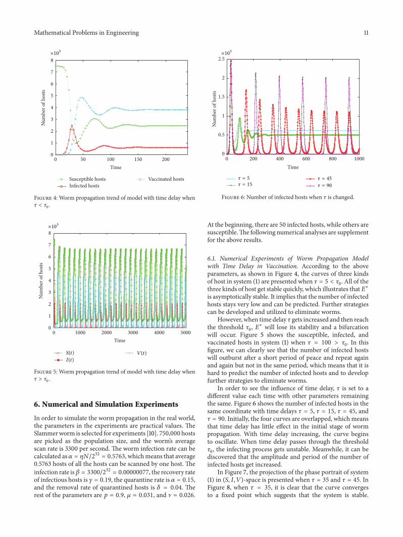pN

120573IS

120574I(t)

120583

D V120574I(t minus 120591)

(1 minus p)N

Figure 1 State transition diagram of delayed model

known worms Based on misuse intrusion detection systemwe propose constant quarantine strategy Although it doesimprove vaccination effect the system is still out of controland Hopf bifurcation is not eliminated either Furthermorethe system fails to detect unknown worms and worm-variants Anomaly intrusion detection system is of helpin detecting these kinds of worm However it is alwaysaccompanied by high false-positive rate

Consequently this paper proposes a worm propagationmodel with impulsive quarantine strategy based on a hybridintrusion detection system that combines both misuse andanomaly intrusion detection to make up for the gaps existingin the two systems After adoption impulsive quarantinestrategy it is clearly proved that Hopf bifurcation is elimi-nated thoroughly so that the system is stable

The rest of the paper is organized as follows In the nextsection related work on time delay and quarantine strategyis introduced Section 3 provides a worm propagation modelwith time delay in vaccination In Section 4 we construct adelayed worm propagation model with constant quarantineand analyze it in detail Then in Section 5 a delayed wormpropagation model using impulsive quarantine strategy isproposed and its analysis is performed Section 6 presentsnumerical analyses and simulation experiments based onSlammer worm Simulation results match well with numer-ical ones Finally Section 7 gives the conclusions

2 Related Work

With the similarity between Internet worms and biologicaldiseases epidemiological models have been widely used inmodeling the propagation of worms [2ndash6] To make theworm transmission in computer network work as in the realword the research within the data-driven framework hasbeen done [7ndash9] Although some human factors are includedthese models cannot restrain worms effectively Thus avariety of containment strategies have been applied to wormpropagationmodels As far as we know the use of quarantinestrategies has produced a great effect on controlling diseasePeople use quarantine strategies widely inworm containmentenlightened by this [10ndash16] In addition some scholars havedone research on time delay [17ndash19]

However previous studies have failed to consider theappropriate quarantine strategy to eliminate the negativeeffect of time delay For instance the pulse quarantinestrategy that Yao has proposed [12] does lead to wormelimination with a relatively low value but time delay isnot considered which leads to Hopf bifurcation so that theworm propagation systemwill be unstable and out of controlIn this paper constant quarantine and impulsive quarantine

strategies are proposed to constrain the worms spreading andeven eliminate Hopf bifurcation

3 Worm Propagation Model withTime Delay in Vaccination

With regard to worms exploiting zero-day vulnerabilitiesnone of the patches could effectively and reliably immunizethe hosts After the hosts are being infected some measuressuch as cutting off the network connection running manualantivirus or setting firewall are taken to remove the wormsWith these measures being carried out the hosts cannotfurther infect other susceptible hosts but they are in factnot vaccinated completely Namely detecting and cleaningworms take a period of time Therefore time delay shouldbe considered in actual conditions Since time delay existsinfected hosts go through a temporary state (delayed) aftervaccination Consequently on the basis of KMmodel we givea worm propagation model with time delay in vaccinationWe assume all hosts are in one of four states susceptible state(S) infected state (I) delayed state (D) and vaccinated state(V) The state transition diagram of the delayed model isgiven in Figure 1

Let 119878(119905) denote the number of susceptible hosts at time 119905119868(119905) denote the number of infected hosts at time 119905119863(119905) denotethe number of delayed hosts at time 119905 and 119881(119905) denote thenumber of vaccinated hosts at time 119905 120573 is the infection rate atwhich susceptible hosts are infected by infected hosts and 120574is the rate of removal of infected from circulation As wormsand worm-variants exist 120583 is the rate that vaccinated hostsback to susceptible hostsThe newborn hosts enter the systemwith the same rate ] of which a portion 1 minus 119901 is recovered byinstalling patches at birth Time delay is denoted by 120591

In order to show it clearly we list in Notations sectionsome frequently used notations in this paper

31 Description of DelayedModel From the above definitionsin the paper we write down the complete differential equa-tions of the delayed model

119889119878 (119905)

119889119905

= 119901]119873 minus 120573119878 (119905) 119868 (119905) minus ]119878 (119905) + 120583119881 (119905)

119889119868 (119905)

119889119905

= 120573119878 (119905) 119868 (119905) minus 120574119868 (119905) minus ]119868 (119905)

119889119863 (119905)

119889119905


119889119881 (119905)

119889119905

= (1 minus 119901) ]119873 + 120574119868 (119905 minus 120591) minus 120583119881 (119905) minus ]119881 (119905)

(1)



119878 (119905) + 119868 (119905) + 119863 (119905) + 119881 (119905) = 119873 (2)





119878 =

120574 + ]120573

119863 = 0

119881 =

120574119868lowast+ (1 minus 119901) ]119873120583 + V

(3)



120574119868lowast+ (1 minus 119901) ]119873120583 + V

= 119873 (4)




119889119878 (119905)

119889119905


minus 120573119878 (119905) 119868 (119905) minus ]119878 (119905)

119889119868 (119905)

119889119905

= 120573119878 (119905) 119868 (119905) minus 120574119868 (119905) minus ]119868 (119905)

119889119863 (119905)

119889119905


(5)


119869 (119864lowast) = (


lowastminus120583

120573119868lowast


0 120574 minus 120574119890minus120582120591

minus]) (6)


119875 (120582) + 119876 (120582) 119890minus120582120591

= 0 (7)

Let

1199012= 120583 + 120573119868



+ 120583 (2] + 120574) + ] (3]2 + 2120574)



1199020= minus120573120583120574119868

lowast

(8)

Then 119875(120582) = 1205823 + 11990121205822+ 1199011120582 + 1199010 119876(120582) = 119902

0



(1198672) 1199012gt 0 119901

11199012minus (1199010+ 1199020) gt 0 119901

0+ 1199020gt 0


1205823+ 11990121205822+ 1199011120582 + (119901

0+ 1199020) = 0 (9)




minus11990121205962+ 1199010+ 1199020cos (120596120591) = 0 (10)

minus1205963+ 1199011120596 minus 1199020sin (120596120591) = 0 (11)

which implies

1205966+ 11986331205964+ 11986321205962+ 1198631= 0 (12)

where

1198633= 1199012

2minus 21199011

1198632= 1199011minus 211990121199010

1198631= 1199012

0minus 1199022

0

(13)


ℎ (119911) = 1199113+ 11986331199112+ 1198632119911 + 119863

1 (14)




3)3 of ℎ(119911)


11199012minus (1199010+ 1199020) gt 0

1199010+ 1199020gt 0 is satisfied


0) and 120591

0is a certain

positive constant




1205823+ 11990121205822+ 1199011120582 + (119901

0+ 1199020) = 0 (15)


1199012gt 0 119901

11199012minus (1199010+ 1199020) gt 0 119901

0+ 1199020gt 0 (16)






easily obtained







(1198673) Δ gt 0 119911








sin(120596120591) in (10) and (11)

120591119896=

1

1205960

arccos[11990121205962

0minus 1199010

1199020

] +

2119896120587

1205960

(119896 = 0 1 2 )

(17)



119896



0is a pair of


119889(Re 120582)119889120591

10038161003816100381610038161003816100381610038161003816120591=120591119896

gt 0 (18)




(

119889120582

119889120591

)

minus1

=

(31205822+ 21199012120582 + 1199011) minus 1199020120591119890minus120582120591

1199020120582119890minus120582120591

(19)

Therefore

sgn [119889Re 120582119889120591

]

120591=120591119896

= sgn[Re(119889120582119889120591

)

minus1

]

120582=1198941205960

= sgn1205962

0

Λ

(31205964

0+ 211986321205962

0+ 1198631)

= sgn1205962

0

Λ

ℎ1015840(1205962

0)

= sgn ℎ1015840 (12059620)

(20)

where Λ = 11990201205962


3) that

ℎ1015840(1205962

0) = 0

Hence

119889(Re 120582)119889120591

10038161003816100381610038161003816100381610038161003816120591=120591119896

gt 0 (21)







2) are

satisfied



0



119896(119896 = 0 1 2 ) where

120591119896is defined by (17)



0 the system






pN

120573 120574I(t)

120583

120574I(t minus 120591)

(1 minus p)N

IS D V

120575120572

Q




119889119878 (119905)

119889119905

= 119901]119873 minus 120573119878 (119905) 119868 (119905) + 120583119881 (119905) minus ]119878 (119905)

119889119868 (119905)

119889119905


119889119863 (119905)

119889119905


119889119876 (119905)

119889119905

= 120572119868 (119905) minus 120575119876 (119905) minus ]119876 (119905)

119889119881 (119905)

119889119905


(22)

Similarly

119878 (119905) + 119868 (119905) + 119863 (119905) + 119876 (119905) + 119881 (119905) = 119873 (23)





119878 =

120574 + 120572 + ]120573

119863 = 0

119876 =

120572

120575 + ]119868lowast

119881 =

120574 + 120572 + ]120583

(

]120573


119901]119873120583

(24)


119878lowast+

120572

120575 + ]119868lowast+ 119868lowast+

120574 + 120572 + ]120583

(

]120573


119901]119873120583

= 119873

(25)



pleted


119889119878 (119905)

119889119905


minus 120573119878 (119905) 119868 (119905) minus ]119878 (119905)

119889119868 (119905)

119889119905


119889119863 (119905)

119889119905


119889119876 (119905)

119889119905

= 120572119868 (119905) minus 120575119876 (119905) minus ]119876 (119905)

(26)


119869 (119864lowast) = (



120573119868lowast


0 120574 minus 120574119890minus120582120591

minus] 0

0 120572 0 minus120575 minus 120583

)

(27)


119875 (120582) + 119876 (120582) 119890minus120582120591

= 0 (28)


Let1199013= 119886 + 119887 + 119888 + ]

1199012= 119886119887 + 119888] + (119886 + 119887) (] + 119888) + 120573119868lowast119889

1199011= 119886119887 (] + 119888) + ]119888 (119886 + 119887) + 120573119868lowast (119889 (] + 119888) + 120583 (120572 + 120574))

1199010= 119886119887119888] + 120573119868lowast (119888119889] + 120572120583] + 119888120583120574)

1199021= minus120583120574120573119868

lowast

1199020= minus120573120583119888120574119868

lowast

(29)

where119886 = 120573119868

lowast+ ] + 120583

119887 = 120574 + 120572 + 120583 minus 120573119878lowast

119888 = 120575 + ]

119889 = 120573119878lowast+ 120583

(30)

then

119875 (120582) = 1205824+ 11990131205823+ 11990121205822+ 1199011120582 + 1199010

119876 (120582) = 1199021120582 + 1199020

(31)



(1198672) 1199013gt 0 119889

1gt 0 119889

2gt 0 (119901

1+ 1199021)1198891minus 1199013

21198892gt 0

where1198891= 11990131199012minus (1199011+ 1199021)

1198892= 1199010+ 1199020

(32)


1205824+ 11990131205823+ 11990121205822+ (1199011+ 1199021) 120582 + (119901

0+ 1199020) = 0 (33)




1205964minus 11990121205962+ 1199010+ 1199021120596 sin (120596120591) + 1199020 cos (120596120591) = 0

minus11990131205963+ 1199011120596 + 1199021120596 cos (120596120591) minus 119902

0sin (120596120591) = 0

(34)

which implies

1205966+ 11986331205964+ 11986321205962+ 1198631= 0 (35)

where

1198633= 1199012

3minus 21199012

1198632= 1199012

2+ 21199010minus 211990111199013

1198631= 1199012

1minus 1199022

1minus 211990121199010

(36)


ℎ (119911) = 1199113+ 11986331199112+ 1198632119911 + 119863

1 (37)




3)3 of ℎ(119911)


1gt 0 and 119889

2gt 0

(1199011+ 1199021)1198891minus 1199013







1205824+ 11990131205823+ 11990121205822+ (1199011+ 1199021) 120582 + (119901

0+ 1199020) = 0 (38)


1199013gt 0 119889

1gt 0 119889

2gt 0 (119901

1+ 1199021) 1198891minus 1199013

21198892gt 0

(39)





easily obtained







(1198673) Δ gt 0 119911


lowast) lt 0







sin(120596120591) in (34)

120591119896

=

1

1205960

arccos [1199020(11990121205962

0minus 1205964

0minus 1199010) + 11990211205960(11990131205963

0minus 11990111205960)

1199022

11205962

0+ 1199022

0

]

+

2119896120587

1205960

(119896 = 0 1 2 )

(40)




119896



0is a pair of


119889 (Re 120582)119889120591

10038161003816100381610038161003816100381610038161003816120591=120591119896

gt 0 (41)




(

119889120582

119889120591

)

minus1

=

(41205823+ 311990131205822+ 21199012120582 + 1199011) + 1199021119890minus120582120591

minus (1199021120582 + 1199020) 120591119890minus120582120591

(1199021120582 + 1199020) 120582119890minus120582120591

(42)Therefore

sgn [119889Re 120582119889120591

]

120591=120591119896

= sgn[Re(119889120582119889120591

)

minus1

]

120582=1198941205960

= sgn1205962

0

Γ

(41205966

0+ 311986331205964

0+ 211986321205962

0+ 1198631)

= sgn1205962

0

Γ

ℎ1015840(1205962

0)

= sgn ℎ1015840 (12059620)

(43)

where Γ = 1199021

21205960

4+ 11990201205960


that ℎ1015840(1205960

2) = 0

Hence119889(Re 120582)119889120591

10038161003816100381610038161003816100381610038161003816120591=120591119896

gt 0 (44)






2) are




120591 gt 1205910



119896(119896 = 0 1 2 )













119889119905

= 119901]119873 minus 120573119878 (119905) 119868 (119905) minus ]119878 (119905) + 120583119881 (119905)

119889119868 (119905)

119889119905


119889119863 (119905)

119889119905


119889119881 (119905)

119889119905


119889119876 (119905)

119889119905

= 120572119868 (119905) minus 120575119876 (119905) minus ]119876 (119905)

119905 = 119899119879

119878 (119899119879+) = 119878 (119899119879


119868 (119899119879+) = 119868 (119899119879



pN

120573 120574I(t)

120583

120574I(t minus 120591)

(1 minus p)N

IS D V

120575120572

Q

1205791

1205792


119863(119899119879+) = 119863 (119899119879

minus)

119876 (119899119879+) = 119876 (119899119879


119881 (119899119879+) = 119881 (119899119879

minus)

119905 = 119899119879

(45)



119878 (119905) + 119868 (119905) + 119863 (119905) + 119876 (119905) + 119881 (119905) = 119873 (46)


119889119878 (119905)

119889119905

= 119901]119873 minus 120573119878 (119905) 119868 (119905) minus ]119878 (119905) + 120583119881 (119905)

119889119868 (119905)

119889119905


119889119863 (119905)

119889119905


119889119881 (119905)

119889119905



119889119876 (119905)

119889119905

= 120572119868 (119905) minus 120575119876 (119905) minus ]119876 (119905)

119905 = 119899119879

119878 (119899119879+) = 119878 (119899119879


119868 (119899119879+) = 119868 (119899119879


119863 (119899119879+) = 119863 (119899119879

minus)

119876 (119899119879+) = 119876 (119899119879


119881 (119899119879+) = 119881 (119899119879

minus)

119905 = 119899119879

(47)


119889119878 (119905)

119889119905

= 119901]119873 minus 120573119878 (119905) 119868 (119905) minus ]119878 (119905) + 120583119881 (119905)

119889119868 (119905)

119889119905


119889119863 (119905)

119889119905


119889119881 (119905)

119889119905



119905 = 119899119879

119878 (119899119879+) = 119878 (119899119879


119868 (119899119879+) = 119868 (119899119879


119863 (119899119879+) = 119863 (119899119879

minus)

119881 (119899119879+) = 119881 (119899119879

minus)

119905 = 119899119879

(48)


Let

119877+= [0infin)

1198774

+= 119885 isin 119877

4 119885 ge 0

(49)




(1206011(120577) 120601

2(120577) 120601

3(120577) 120601

4(120577)) isin 119862

+= 119862 ([minus120596 0] 119877

4

+)

120601119894(0) gt 0 119894 = 1 2 3 4

(50)





0


+rarr 1198774

+ 119885(119905) is continuous on [119899119879 (119899 + 1)119879]

119896 isin 119885+ and 119885(119899119879

+) = lim




Denote

Ω = (119878 119868 119863 119881) isin 1198774| 119878 ge 0 119868 ge 0 119863 ge 0 119881 ge 0 (51)



(119905) = 1198861119909 (119905 minus 120596) minus 119886

2119909 (119905) (52)


We have

(i) if 1198861lt 1198862 then lim

119905rarrinfin119909(119905) = 0

(ii) if 1198861gt 1198862 then lim

119905rarrinfin119909(119905) = +infin



119889119878 (119905)

119889119905

= 119901]119873 minus 120573119878 (119905) 119868 (119905) minus ]119878 (119905) + 120583119881 (119905)

119889119863 (119905)

119889119905


119889119881 (119905)

119889119905



119905 = 119899119879

119878 (119899119879+) = 119878 (119899119879


119863 (119899119879+) = 119863 (119899119879

minus)

119881 (119899119879+) = 119881 (119899119879

minus)

119905 = 119899119879

(53)




119878 (119905) = 119901119873 + (119878lowastminus 119901119873) 119890

minus](119905minus119899119879) 119899119879 lt 119905 le (119899 + 1) 119879

(54)


119878lowast=

119901119873 (1 minus 1205791) (1 minus 119890

minus]119879)


(55)




120575119878(119905))(120575 + ] + 120583)



119877lowast=

120573119901119873 (1 minus 1205791) (1 minus 119890

minus]119879)


)

(56)


such that

120573(

119901119873(1 minus 1205791) (1 minus 119890

minus]119879)


+ 1205760) lt ] + 120574 + 120572 (57)


119878 (119905) le 119901]119873 minus ]119878 (119905) + 120583119881 (119905) (58)


(119905) = 119901]119873 minus ]119909 (119905) 119905 = 119899119879

119909 (119899119879+) = (1 minus 120579

1) 119909 (119899119879

minus) 119905 = 119899119879

(59)


119909 (119905) = 119878 (119905) = 119901119873 + (119878lowastminus 119901119873) 119890

minus](119905minus119899119879)

119899119879 lt 119905 le (119899 + 1) 119879

(60)



119901119873 (1 minus 1205791) (1 minus 119890

minus]119879)



0gt 0 119909(119905) be




1gt 0 such that

119878 (119905) lt 119909 (119905) lt 119909 (119905) + 1205760 119899119879 lt 119905 le (119899 + 1) 119879 (62)

that is

119878 (119905) lt 119878 (119905) + 1205760le

119901119873 (1 minus 1205791) (1 minus 119890

minus]119879)


+ 1205760≜ 119878119872

119899119879 lt 119905 le (119899 + 1) 119879 119899 gt 1198991

(63)


119868 (119905) le 120573119878119872119868 (119905) minus (] + 120574 + 120572) 119868 (119905) 119905 gt 119899119879 119899 gt 119899

1 (64)


119910 (119905) = 120573119878119872119910 (119905) minus (] + 120574 + 120572) 119910 (119905) 119905 gt 119899119879 119899 gt 119899

1

(65)








119905rarrinfin119910(119905) =


lim119905rarrinfin

119868 (119905) = 0 (66)



1for all 119905 gt 119899

2119879


(119905) lt 1205741205761minus ]119863 (119905) for 119905 gt 119899

2119879 (67)


(119905) = 1205741205761minus ]119911 (119905) (68)



3119879

119863 (119905) le

1205741205761

]+ 1205761 (69)



lim119905rarrinfin

119863 (119905) = 0 (70)


119878 (119905) ge 119901]119873 minus (] + 1205731205761) 119878 (119905) for 119899 gt 119899

3119879 (71)


(119905) = 119901]119873 minus (] + 1205731205761) 119906 (119905) 119905 = 119899119879

119906 (119899119879+) = (1 minus 120579

1) 119906 (119899119879

minus) 119905 = 119899119879

(72)


(119905) =

119901]119873] + 120573120576

1


119901]119873] + 120573120576

1

) 119890minus(]+1205731205761)(119905minus119899119879)

119899119879 lt 119905 le (119899 + 1) 119879

(73)


119906lowast=

119901]119873] + 120573120576

1

(1 minus 1205791) (1 minus 119890

minus(]+1205731205761)119879)


(74)



119878 (119905) gt (119905) minus 1205761 119899119879 lt 119905 le (119899 + 1) 119899 gt 119899

4 (75)


have that

119878 (119905) = 119901119873(1 minus

1205791(1 minus 119890

minus]119879)


)

119899119879 lt 119905 le (119899 + 1) 119879

(76)


lim119905rarrinfin

119878 (119905) = 119878 (119905) (77)



for 119905 gt 1198994119879


119881 (119905) lt

[120575 + (1 minus 119901) ]]119873 minus 120575119878 (119905)

120575 + ] + 120583+ 1205761

for 119905 gt 1198995119879 (79)


119881 (119905) gt

[120575 + (1 minus 119901) ]]119873 minus 120575119878 (119905)

120575 + ] + 120583minus 1205761

for 119905 gt 1198996119879 (80)



119881 (119905)

= ( [120575 + (1 minus 119901) ]]119873

minus120575119901119873(1 minus

(1205791(1 minus 119890

minus]119879))


119890minus](119905minus119899119879)

))

times (120575 + ] + 120583)minus1

(81)



0 50 100 150 2000

1

2

3

4

5

6

7

8

Time

Num

ber o

f hos

ts


Vaccinated hosts

times105


0 1000 2000 3000 4000 50000

1

2

3

4

5

6

7

8

Time

Num

ber o

f hos

ts

times105

S(t)

I(t)

V(t)




0 200 400 600 800 10000

05

1

15

2

25

Time

Num

ber o

f hos

ts

120591 = 5120591 = 15

120591 = 45

120591 = 90

times105




0 All of the





0 In this






4

2

50

0 0

5

10

times105

times105

times105

S(t)

I(t)

V(t)

(a) 120591 = 35

4

2

50

0 0

5

10

times105

times105

S(t)

I(t)

V(t)

times105

(b) 120591 = 45


0 1 2 30

2

4

6

8times105

times105

S(t)

I(t)

(a) 120591 = 35

0 1 2 30

2

4

6

8times105

times105

S(t)

I(t)

(b) 120591 = 45



0= 38







0 20 40 60 80 1000

05

1

15

2

25

Hopfbifurcation

I(t)

120591

times105


012345678

Num

ber o

f ho

sts

0 50 100 150 200 250 300 350 400Time



times105


0

0 1000 2000 3000 4000 50000

1

2

3

4

5

6

7

8

Time

Num

ber o

f hos

ts

S(t)

I(t)

V(t)

times105


0

0 1000 2000 3000 4000 50000

05

1

15

2

25

3

35

4

Time

Num

ber o

f inf

ecte

d ho

sts


times105


0




0 In this









5

102

0 0

42

4

6

8times105

times105

times104

S(t)

I(t)

V(t)

(a) 120591 = 40

42

4

6

8times105

S(t)

2

0

times105

V(t)5

10

0

times104

I(t)

(b) 120591 = 55


0 2 4 6 82

3

4

5

6

7

8times105

times104

S(t)

I(t)

(a) 120591 = 40

0 5 102

3

4

5

6

7

8times105

times104

S(t)

I(t)

(b) 120591 = 55


1205791= 000002315 and 120579










0 10 20 30 40 50 60 70 80 900

1

2

3

4

5


times104

120591


0 100 200 300 4000

1

2

3

4

5

6

7

8

Time

Num

ber o

f hos

ts



times105


0


7 Conclusions


0

2

4

6

8

Time

Num

ber o

f hos

ts

times105

times104


Vaccinated hosts

0 1 2 3 4


0

0 5000 10000 150000

05

1

15

2

25

3

Time

Num

ber o

f inf

ecte

d ho

sts



times105


0






Time

Numerical curve

0 100 200 300 4000

2

4

6

8

10

Num

ber o

f inf

ecte

d ho

sts

Simulation curve

times104

(a) 120591 lt 1205910

0 500 1000 1500 2000 2500 3000 35000

2

4

6

8

10

Time

Num

ber o

f inf

ecte

d ho

sts


times104

(b) 120591 gt 1205910



0 100 200 300 400 5000

2

4

6

8

10

Time

Num

ber o

f inf

ecte

d ho

sts

times104

(a)


0 05 1 15 20

2

4

6

8

10

Time

Num

ber o

f inf

ecte

d ho

sts

times104

times104

(b)











Notations




worms



Acknowledgments


References





































Volume 2014




Journal of











Journal of


Function Spaces






Algebra











119878 (119905) + 119868 (119905) + 119863 (119905) + 119881 (119905) = 119873 (2)





119878 =

120574 + ]120573

119863 = 0

119881 =

120574119868lowast+ (1 minus 119901) ]119873120583 + V

(3)



120574119868lowast+ (1 minus 119901) ]119873120583 + V

= 119873 (4)




119889119878 (119905)

119889119905


minus 120573119878 (119905) 119868 (119905) minus ]119878 (119905)

119889119868 (119905)

119889119905

= 120573119878 (119905) 119868 (119905) minus 120574119868 (119905) minus ]119868 (119905)

119889119863 (119905)

119889119905


(5)


119869 (119864lowast) = (


lowastminus120583

120573119868lowast


0 120574 minus 120574119890minus120582120591

minus]) (6)


119875 (120582) + 119876 (120582) 119890minus120582120591

= 0 (7)

Let

1199012= 120583 + 120573119868



+ 120583 (2] + 120574) + ] (3]2 + 2120574)



1199020= minus120573120583120574119868

lowast

(8)

Then 119875(120582) = 1205823 + 11990121205822+ 1199011120582 + 1199010 119876(120582) = 119902

0



(1198672) 1199012gt 0 119901

11199012minus (1199010+ 1199020) gt 0 119901

0+ 1199020gt 0


1205823+ 11990121205822+ 1199011120582 + (119901

0+ 1199020) = 0 (9)




minus11990121205962+ 1199010+ 1199020cos (120596120591) = 0 (10)

minus1205963+ 1199011120596 minus 1199020sin (120596120591) = 0 (11)

which implies

1205966+ 11986331205964+ 11986321205962+ 1198631= 0 (12)

where

1198633= 1199012

2minus 21199011

1198632= 1199011minus 211990121199010

1198631= 1199012

0minus 1199022

0

(13)


ℎ (119911) = 1199113+ 11986331199112+ 1198632119911 + 119863

1 (14)




3)3 of ℎ(119911)


11199012minus (1199010+ 1199020) gt 0

1199010+ 1199020gt 0 is satisfied


0) and 120591

0is a certain

positive constant




1205823+ 11990121205822+ 1199011120582 + (119901

0+ 1199020) = 0 (15)


1199012gt 0 119901

11199012minus (1199010+ 1199020) gt 0 119901

0+ 1199020gt 0 (16)






easily obtained







(1198673) Δ gt 0 119911








sin(120596120591) in (10) and (11)

120591119896=

1

1205960

arccos[11990121205962

0minus 1199010

1199020

] +

2119896120587

1205960

(119896 = 0 1 2 )

(17)



119896



0is a pair of


119889(Re 120582)119889120591

10038161003816100381610038161003816100381610038161003816120591=120591119896

gt 0 (18)




(

119889120582

119889120591

)

minus1

=

(31205822+ 21199012120582 + 1199011) minus 1199020120591119890minus120582120591

1199020120582119890minus120582120591

(19)

Therefore

sgn [119889Re 120582119889120591

]

120591=120591119896

= sgn[Re(119889120582119889120591

)

minus1

]

120582=1198941205960

= sgn1205962

0

Λ

(31205964

0+ 211986321205962

0+ 1198631)

= sgn1205962

0

Λ

ℎ1015840(1205962

0)

= sgn ℎ1015840 (12059620)

(20)

where Λ = 11990201205962


3) that

ℎ1015840(1205962

0) = 0

Hence

119889(Re 120582)119889120591

10038161003816100381610038161003816100381610038161003816120591=120591119896

gt 0 (21)







2) are

satisfied



0



119896(119896 = 0 1 2 ) where

120591119896is defined by (17)



0 the system






pN

120573 120574I(t)

120583

120574I(t minus 120591)

(1 minus p)N

IS D V

120575120572

Q




119889119878 (119905)

119889119905

= 119901]119873 minus 120573119878 (119905) 119868 (119905) + 120583119881 (119905) minus ]119878 (119905)

119889119868 (119905)

119889119905


119889119863 (119905)

119889119905


119889119876 (119905)

119889119905

= 120572119868 (119905) minus 120575119876 (119905) minus ]119876 (119905)

119889119881 (119905)

119889119905


(22)

Similarly

119878 (119905) + 119868 (119905) + 119863 (119905) + 119876 (119905) + 119881 (119905) = 119873 (23)





119878 =

120574 + 120572 + ]120573

119863 = 0

119876 =

120572

120575 + ]119868lowast

119881 =

120574 + 120572 + ]120583

(

]120573


119901]119873120583

(24)


119878lowast+

120572

120575 + ]119868lowast+ 119868lowast+

120574 + 120572 + ]120583

(

]120573


119901]119873120583

= 119873

(25)



pleted


119889119878 (119905)

119889119905


minus 120573119878 (119905) 119868 (119905) minus ]119878 (119905)

119889119868 (119905)

119889119905


119889119863 (119905)

119889119905


119889119876 (119905)

119889119905

= 120572119868 (119905) minus 120575119876 (119905) minus ]119876 (119905)

(26)


119869 (119864lowast) = (



120573119868lowast


0 120574 minus 120574119890minus120582120591

minus] 0

0 120572 0 minus120575 minus 120583

)

(27)


119875 (120582) + 119876 (120582) 119890minus120582120591

= 0 (28)


Let1199013= 119886 + 119887 + 119888 + ]

1199012= 119886119887 + 119888] + (119886 + 119887) (] + 119888) + 120573119868lowast119889

1199011= 119886119887 (] + 119888) + ]119888 (119886 + 119887) + 120573119868lowast (119889 (] + 119888) + 120583 (120572 + 120574))

1199010= 119886119887119888] + 120573119868lowast (119888119889] + 120572120583] + 119888120583120574)

1199021= minus120583120574120573119868

lowast

1199020= minus120573120583119888120574119868

lowast

(29)

where119886 = 120573119868

lowast+ ] + 120583

119887 = 120574 + 120572 + 120583 minus 120573119878lowast

119888 = 120575 + ]

119889 = 120573119878lowast+ 120583

(30)

then

119875 (120582) = 1205824+ 11990131205823+ 11990121205822+ 1199011120582 + 1199010

119876 (120582) = 1199021120582 + 1199020

(31)



(1198672) 1199013gt 0 119889

1gt 0 119889

2gt 0 (119901

1+ 1199021)1198891minus 1199013

21198892gt 0

where1198891= 11990131199012minus (1199011+ 1199021)

1198892= 1199010+ 1199020

(32)


1205824+ 11990131205823+ 11990121205822+ (1199011+ 1199021) 120582 + (119901

0+ 1199020) = 0 (33)




1205964minus 11990121205962+ 1199010+ 1199021120596 sin (120596120591) + 1199020 cos (120596120591) = 0

minus11990131205963+ 1199011120596 + 1199021120596 cos (120596120591) minus 119902

0sin (120596120591) = 0

(34)

which implies

1205966+ 11986331205964+ 11986321205962+ 1198631= 0 (35)

where

1198633= 1199012

3minus 21199012

1198632= 1199012

2+ 21199010minus 211990111199013

1198631= 1199012

1minus 1199022

1minus 211990121199010

(36)


ℎ (119911) = 1199113+ 11986331199112+ 1198632119911 + 119863

1 (37)




3)3 of ℎ(119911)


1gt 0 and 119889

2gt 0

(1199011+ 1199021)1198891minus 1199013







1205824+ 11990131205823+ 11990121205822+ (1199011+ 1199021) 120582 + (119901

0+ 1199020) = 0 (38)


1199013gt 0 119889

1gt 0 119889

2gt 0 (119901

1+ 1199021) 1198891minus 1199013

21198892gt 0

(39)





easily obtained







(1198673) Δ gt 0 119911


lowast) lt 0







sin(120596120591) in (34)

120591119896

=

1

1205960

arccos [1199020(11990121205962

0minus 1205964

0minus 1199010) + 11990211205960(11990131205963

0minus 11990111205960)

1199022

11205962

0+ 1199022

0

]

+

2119896120587

1205960

(119896 = 0 1 2 )

(40)




119896



0is a pair of


119889 (Re 120582)119889120591

10038161003816100381610038161003816100381610038161003816120591=120591119896

gt 0 (41)




(

119889120582

119889120591

)

minus1

=

(41205823+ 311990131205822+ 21199012120582 + 1199011) + 1199021119890minus120582120591

minus (1199021120582 + 1199020) 120591119890minus120582120591

(1199021120582 + 1199020) 120582119890minus120582120591

(42)Therefore

sgn [119889Re 120582119889120591

]

120591=120591119896

= sgn[Re(119889120582119889120591

)

minus1

]

120582=1198941205960

= sgn1205962

0

Γ

(41205966

0+ 311986331205964

0+ 211986321205962

0+ 1198631)

= sgn1205962

0

Γ

ℎ1015840(1205962

0)

= sgn ℎ1015840 (12059620)

(43)

where Γ = 1199021

21205960

4+ 11990201205960


that ℎ1015840(1205960

2) = 0

Hence119889(Re 120582)119889120591

10038161003816100381610038161003816100381610038161003816120591=120591119896

gt 0 (44)






2) are




120591 gt 1205910



119896(119896 = 0 1 2 )













119889119905

= 119901]119873 minus 120573119878 (119905) 119868 (119905) minus ]119878 (119905) + 120583119881 (119905)

119889119868 (119905)

119889119905


119889119863 (119905)

119889119905


119889119881 (119905)

119889119905


119889119876 (119905)

119889119905

= 120572119868 (119905) minus 120575119876 (119905) minus ]119876 (119905)

119905 = 119899119879

119878 (119899119879+) = 119878 (119899119879


119868 (119899119879+) = 119868 (119899119879



pN

120573 120574I(t)

120583

120574I(t minus 120591)

(1 minus p)N

IS D V

120575120572

Q

1205791

1205792


119863(119899119879+) = 119863 (119899119879

minus)

119876 (119899119879+) = 119876 (119899119879


119881 (119899119879+) = 119881 (119899119879

minus)

119905 = 119899119879

(45)



119878 (119905) + 119868 (119905) + 119863 (119905) + 119876 (119905) + 119881 (119905) = 119873 (46)


119889119878 (119905)

119889119905

= 119901]119873 minus 120573119878 (119905) 119868 (119905) minus ]119878 (119905) + 120583119881 (119905)

119889119868 (119905)

119889119905


119889119863 (119905)

119889119905


119889119881 (119905)

119889119905



119889119876 (119905)

119889119905

= 120572119868 (119905) minus 120575119876 (119905) minus ]119876 (119905)

119905 = 119899119879

119878 (119899119879+) = 119878 (119899119879


119868 (119899119879+) = 119868 (119899119879


119863 (119899119879+) = 119863 (119899119879

minus)

119876 (119899119879+) = 119876 (119899119879


119881 (119899119879+) = 119881 (119899119879

minus)

119905 = 119899119879

(47)


119889119878 (119905)

119889119905

= 119901]119873 minus 120573119878 (119905) 119868 (119905) minus ]119878 (119905) + 120583119881 (119905)

119889119868 (119905)

119889119905


119889119863 (119905)

119889119905


119889119881 (119905)

119889119905



119905 = 119899119879

119878 (119899119879+) = 119878 (119899119879


119868 (119899119879+) = 119868 (119899119879


119863 (119899119879+) = 119863 (119899119879

minus)

119881 (119899119879+) = 119881 (119899119879

minus)

119905 = 119899119879

(48)


Let

119877+= [0infin)

1198774

+= 119885 isin 119877

4 119885 ge 0

(49)




(1206011(120577) 120601

2(120577) 120601

3(120577) 120601

4(120577)) isin 119862

+= 119862 ([minus120596 0] 119877

4

+)

120601119894(0) gt 0 119894 = 1 2 3 4

(50)





0


+rarr 1198774

+ 119885(119905) is continuous on [119899119879 (119899 + 1)119879]

119896 isin 119885+ and 119885(119899119879

+) = lim




Denote

Ω = (119878 119868 119863 119881) isin 1198774| 119878 ge 0 119868 ge 0 119863 ge 0 119881 ge 0 (51)



(119905) = 1198861119909 (119905 minus 120596) minus 119886

2119909 (119905) (52)


We have

(i) if 1198861lt 1198862 then lim

119905rarrinfin119909(119905) = 0

(ii) if 1198861gt 1198862 then lim

119905rarrinfin119909(119905) = +infin



119889119878 (119905)

119889119905

= 119901]119873 minus 120573119878 (119905) 119868 (119905) minus ]119878 (119905) + 120583119881 (119905)

119889119863 (119905)

119889119905


119889119881 (119905)

119889119905



119905 = 119899119879

119878 (119899119879+) = 119878 (119899119879


119863 (119899119879+) = 119863 (119899119879

minus)

119881 (119899119879+) = 119881 (119899119879

minus)

119905 = 119899119879

(53)




119878 (119905) = 119901119873 + (119878lowastminus 119901119873) 119890

minus](119905minus119899119879) 119899119879 lt 119905 le (119899 + 1) 119879

(54)


119878lowast=

119901119873 (1 minus 1205791) (1 minus 119890

minus]119879)


(55)




120575119878(119905))(120575 + ] + 120583)



119877lowast=

120573119901119873 (1 minus 1205791) (1 minus 119890

minus]119879)


)

(56)


such that

120573(

119901119873(1 minus 1205791) (1 minus 119890

minus]119879)


+ 1205760) lt ] + 120574 + 120572 (57)


119878 (119905) le 119901]119873 minus ]119878 (119905) + 120583119881 (119905) (58)


(119905) = 119901]119873 minus ]119909 (119905) 119905 = 119899119879

119909 (119899119879+) = (1 minus 120579

1) 119909 (119899119879

minus) 119905 = 119899119879

(59)


119909 (119905) = 119878 (119905) = 119901119873 + (119878lowastminus 119901119873) 119890

minus](119905minus119899119879)

119899119879 lt 119905 le (119899 + 1) 119879

(60)



119901119873 (1 minus 1205791) (1 minus 119890

minus]119879)



0gt 0 119909(119905) be




1gt 0 such that

119878 (119905) lt 119909 (119905) lt 119909 (119905) + 1205760 119899119879 lt 119905 le (119899 + 1) 119879 (62)

that is

119878 (119905) lt 119878 (119905) + 1205760le

119901119873 (1 minus 1205791) (1 minus 119890

minus]119879)


+ 1205760≜ 119878119872

119899119879 lt 119905 le (119899 + 1) 119879 119899 gt 1198991

(63)


119868 (119905) le 120573119878119872119868 (119905) minus (] + 120574 + 120572) 119868 (119905) 119905 gt 119899119879 119899 gt 119899

1 (64)


119910 (119905) = 120573119878119872119910 (119905) minus (] + 120574 + 120572) 119910 (119905) 119905 gt 119899119879 119899 gt 119899

1

(65)








119905rarrinfin119910(119905) =


lim119905rarrinfin

119868 (119905) = 0 (66)



1for all 119905 gt 119899

2119879


(119905) lt 1205741205761minus ]119863 (119905) for 119905 gt 119899

2119879 (67)


(119905) = 1205741205761minus ]119911 (119905) (68)



3119879

119863 (119905) le

1205741205761

]+ 1205761 (69)



lim119905rarrinfin

119863 (119905) = 0 (70)


119878 (119905) ge 119901]119873 minus (] + 1205731205761) 119878 (119905) for 119899 gt 119899

3119879 (71)


(119905) = 119901]119873 minus (] + 1205731205761) 119906 (119905) 119905 = 119899119879

119906 (119899119879+) = (1 minus 120579

1) 119906 (119899119879

minus) 119905 = 119899119879

(72)


(119905) =

119901]119873] + 120573120576

1


119901]119873] + 120573120576

1

) 119890minus(]+1205731205761)(119905minus119899119879)

119899119879 lt 119905 le (119899 + 1) 119879

(73)


119906lowast=

119901]119873] + 120573120576

1

(1 minus 1205791) (1 minus 119890

minus(]+1205731205761)119879)


(74)



119878 (119905) gt (119905) minus 1205761 119899119879 lt 119905 le (119899 + 1) 119899 gt 119899

4 (75)


have that

119878 (119905) = 119901119873(1 minus

1205791(1 minus 119890

minus]119879)


)

119899119879 lt 119905 le (119899 + 1) 119879

(76)


lim119905rarrinfin

119878 (119905) = 119878 (119905) (77)



for 119905 gt 1198994119879


119881 (119905) lt

[120575 + (1 minus 119901) ]]119873 minus 120575119878 (119905)

120575 + ] + 120583+ 1205761

for 119905 gt 1198995119879 (79)


119881 (119905) gt

[120575 + (1 minus 119901) ]]119873 minus 120575119878 (119905)

120575 + ] + 120583minus 1205761

for 119905 gt 1198996119879 (80)



119881 (119905)

= ( [120575 + (1 minus 119901) ]]119873

minus120575119901119873(1 minus

(1205791(1 minus 119890

minus]119879))


119890minus](119905minus119899119879)

))

times (120575 + ] + 120583)minus1

(81)



0 50 100 150 2000

1

2

3

4

5

6

7

8

Time

Num

ber o

f hos

ts


Vaccinated hosts

times105


0 1000 2000 3000 4000 50000

1

2

3

4

5

6

7

8

Time

Num

ber o

f hos

ts

times105

S(t)

I(t)

V(t)




0 200 400 600 800 10000

05

1

15

2

25

Time

Num

ber o

f hos

ts

120591 = 5120591 = 15

120591 = 45

120591 = 90

times105




0 All of the





0 In this






4

2

50

0 0

5

10

times105

times105

times105

S(t)

I(t)

V(t)

(a) 120591 = 35

4

2

50

0 0

5

10

times105

times105

S(t)

I(t)

V(t)

times105

(b) 120591 = 45


0 1 2 30

2

4

6

8times105

times105

S(t)

I(t)

(a) 120591 = 35

0 1 2 30

2

4

6

8times105

times105

S(t)

I(t)

(b) 120591 = 45



0= 38







0 20 40 60 80 1000

05

1

15

2

25

Hopfbifurcation

I(t)

120591

times105


012345678

Num

ber o

f ho

sts

0 50 100 150 200 250 300 350 400Time



times105


0

0 1000 2000 3000 4000 50000

1

2

3

4

5

6

7

8

Time

Num

ber o

f hos

ts

S(t)

I(t)

V(t)

times105


0

0 1000 2000 3000 4000 50000

05

1

15

2

25

3

35

4

Time

Num

ber o

f inf

ecte

d ho

sts


times105


0




0 In this









5

102

0 0

42

4

6

8times105

times105

times104

S(t)

I(t)

V(t)

(a) 120591 = 40

42

4

6

8times105

S(t)

2

0

times105

V(t)5

10

0

times104

I(t)

(b) 120591 = 55


0 2 4 6 82

3

4

5

6

7

8times105

times104

S(t)

I(t)

(a) 120591 = 40

0 5 102

3

4

5

6

7

8times105

times104

S(t)

I(t)

(b) 120591 = 55


1205791= 000002315 and 120579










0 10 20 30 40 50 60 70 80 900

1

2

3

4

5


times104

120591


0 100 200 300 4000

1

2

3

4

5

6

7

8

Time

Num

ber o

f hos

ts



times105


0


7 Conclusions


0

2

4

6

8

Time

Num

ber o

f hos

ts

times105

times104


Vaccinated hosts

0 1 2 3 4


0

0 5000 10000 150000

05

1

15

2

25

3

Time

Num

ber o

f inf

ecte

d ho

sts



times105


0






Time

Numerical curve

0 100 200 300 4000

2

4

6

8

10

Num

ber o

f inf

ecte

d ho

sts

Simulation curve

times104

(a) 120591 lt 1205910

0 500 1000 1500 2000 2500 3000 35000

2

4

6

8

10

Time

Num

ber o

f inf

ecte

d ho

sts


times104

(b) 120591 gt 1205910



0 100 200 300 400 5000

2

4

6

8

10

Time

Num

ber o

f inf

ecte

d ho

sts

times104

(a)


0 05 1 15 20

2

4

6

8

10

Time

Num

ber o

f inf

ecte

d ho

sts

times104

times104

(b)











Notations




worms



Acknowledgments


References





































Volume 2014




Journal of











Journal of


Function Spaces






Algebra












1205823+ 11990121205822+ 1199011120582 + (119901

0+ 1199020) = 0 (15)


1199012gt 0 119901

11199012minus (1199010+ 1199020) gt 0 119901

0+ 1199020gt 0 (16)






easily obtained







(1198673) Δ gt 0 119911








sin(120596120591) in (10) and (11)

120591119896=

1

1205960

arccos[11990121205962

0minus 1199010

1199020

] +

2119896120587

1205960

(119896 = 0 1 2 )

(17)



119896



0is a pair of


119889(Re 120582)119889120591

10038161003816100381610038161003816100381610038161003816120591=120591119896

gt 0 (18)




(

119889120582

119889120591

)

minus1

=

(31205822+ 21199012120582 + 1199011) minus 1199020120591119890minus120582120591

1199020120582119890minus120582120591

(19)

Therefore

sgn [119889Re 120582119889120591

]

120591=120591119896

= sgn[Re(119889120582119889120591

)

minus1

]

120582=1198941205960

= sgn1205962

0

Λ

(31205964

0+ 211986321205962

0+ 1198631)

= sgn1205962

0

Λ

ℎ1015840(1205962

0)

= sgn ℎ1015840 (12059620)

(20)

where Λ = 11990201205962


3) that

ℎ1015840(1205962

0) = 0

Hence

119889(Re 120582)119889120591

10038161003816100381610038161003816100381610038161003816120591=120591119896

gt 0 (21)







2) are

satisfied



0



119896(119896 = 0 1 2 ) where

120591119896is defined by (17)



0 the system






pN

120573 120574I(t)

120583

120574I(t minus 120591)

(1 minus p)N

IS D V

120575120572

Q




119889119878 (119905)

119889119905

= 119901]119873 minus 120573119878 (119905) 119868 (119905) + 120583119881 (119905) minus ]119878 (119905)

119889119868 (119905)

119889119905


119889119863 (119905)

119889119905


119889119876 (119905)

119889119905

= 120572119868 (119905) minus 120575119876 (119905) minus ]119876 (119905)

119889119881 (119905)

119889119905


(22)

Similarly

119878 (119905) + 119868 (119905) + 119863 (119905) + 119876 (119905) + 119881 (119905) = 119873 (23)





119878 =

120574 + 120572 + ]120573

119863 = 0

119876 =

120572

120575 + ]119868lowast

119881 =

120574 + 120572 + ]120583

(

]120573


119901]119873120583

(24)


119878lowast+

120572

120575 + ]119868lowast+ 119868lowast+

120574 + 120572 + ]120583

(

]120573


119901]119873120583

= 119873

(25)



pleted


119889119878 (119905)

119889119905


minus 120573119878 (119905) 119868 (119905) minus ]119878 (119905)

119889119868 (119905)

119889119905


119889119863 (119905)

119889119905


119889119876 (119905)

119889119905

= 120572119868 (119905) minus 120575119876 (119905) minus ]119876 (119905)

(26)


119869 (119864lowast) = (



120573119868lowast


0 120574 minus 120574119890minus120582120591

minus] 0

0 120572 0 minus120575 minus 120583

)

(27)


119875 (120582) + 119876 (120582) 119890minus120582120591

= 0 (28)


Let1199013= 119886 + 119887 + 119888 + ]

1199012= 119886119887 + 119888] + (119886 + 119887) (] + 119888) + 120573119868lowast119889

1199011= 119886119887 (] + 119888) + ]119888 (119886 + 119887) + 120573119868lowast (119889 (] + 119888) + 120583 (120572 + 120574))

1199010= 119886119887119888] + 120573119868lowast (119888119889] + 120572120583] + 119888120583120574)

1199021= minus120583120574120573119868

lowast

1199020= minus120573120583119888120574119868

lowast

(29)

where119886 = 120573119868

lowast+ ] + 120583

119887 = 120574 + 120572 + 120583 minus 120573119878lowast

119888 = 120575 + ]

119889 = 120573119878lowast+ 120583

(30)

then

119875 (120582) = 1205824+ 11990131205823+ 11990121205822+ 1199011120582 + 1199010

119876 (120582) = 1199021120582 + 1199020

(31)



(1198672) 1199013gt 0 119889

1gt 0 119889

2gt 0 (119901

1+ 1199021)1198891minus 1199013

21198892gt 0

where1198891= 11990131199012minus (1199011+ 1199021)

1198892= 1199010+ 1199020

(32)


1205824+ 11990131205823+ 11990121205822+ (1199011+ 1199021) 120582 + (119901

0+ 1199020) = 0 (33)




1205964minus 11990121205962+ 1199010+ 1199021120596 sin (120596120591) + 1199020 cos (120596120591) = 0

minus11990131205963+ 1199011120596 + 1199021120596 cos (120596120591) minus 119902

0sin (120596120591) = 0

(34)

which implies

1205966+ 11986331205964+ 11986321205962+ 1198631= 0 (35)

where

1198633= 1199012

3minus 21199012

1198632= 1199012

2+ 21199010minus 211990111199013

1198631= 1199012

1minus 1199022

1minus 211990121199010

(36)


ℎ (119911) = 1199113+ 11986331199112+ 1198632119911 + 119863

1 (37)




3)3 of ℎ(119911)


1gt 0 and 119889

2gt 0

(1199011+ 1199021)1198891minus 1199013







1205824+ 11990131205823+ 11990121205822+ (1199011+ 1199021) 120582 + (119901

0+ 1199020) = 0 (38)


1199013gt 0 119889

1gt 0 119889

2gt 0 (119901

1+ 1199021) 1198891minus 1199013

21198892gt 0

(39)





easily obtained







(1198673) Δ gt 0 119911


lowast) lt 0







sin(120596120591) in (34)

120591119896

=

1

1205960

arccos [1199020(11990121205962

0minus 1205964

0minus 1199010) + 11990211205960(11990131205963

0minus 11990111205960)

1199022

11205962

0+ 1199022

0

]

+

2119896120587

1205960

(119896 = 0 1 2 )

(40)




119896



0is a pair of


119889 (Re 120582)119889120591

10038161003816100381610038161003816100381610038161003816120591=120591119896

gt 0 (41)




(

119889120582

119889120591

)

minus1

=

(41205823+ 311990131205822+ 21199012120582 + 1199011) + 1199021119890minus120582120591

minus (1199021120582 + 1199020) 120591119890minus120582120591

(1199021120582 + 1199020) 120582119890minus120582120591

(42)Therefore

sgn [119889Re 120582119889120591

]

120591=120591119896

= sgn[Re(119889120582119889120591

)

minus1

]

120582=1198941205960

= sgn1205962

0

Γ

(41205966

0+ 311986331205964

0+ 211986321205962

0+ 1198631)

= sgn1205962

0

Γ

ℎ1015840(1205962

0)

= sgn ℎ1015840 (12059620)

(43)

where Γ = 1199021

21205960

4+ 11990201205960


that ℎ1015840(1205960

2) = 0

Hence119889(Re 120582)119889120591

10038161003816100381610038161003816100381610038161003816120591=120591119896

gt 0 (44)






2) are




120591 gt 1205910



119896(119896 = 0 1 2 )













119889119905

= 119901]119873 minus 120573119878 (119905) 119868 (119905) minus ]119878 (119905) + 120583119881 (119905)

119889119868 (119905)

119889119905


119889119863 (119905)

119889119905


119889119881 (119905)

119889119905


119889119876 (119905)

119889119905

= 120572119868 (119905) minus 120575119876 (119905) minus ]119876 (119905)

119905 = 119899119879

119878 (119899119879+) = 119878 (119899119879


119868 (119899119879+) = 119868 (119899119879



pN

120573 120574I(t)

120583

120574I(t minus 120591)

(1 minus p)N

IS D V

120575120572

Q

1205791

1205792


119863(119899119879+) = 119863 (119899119879

minus)

119876 (119899119879+) = 119876 (119899119879


119881 (119899119879+) = 119881 (119899119879

minus)

119905 = 119899119879

(45)



119878 (119905) + 119868 (119905) + 119863 (119905) + 119876 (119905) + 119881 (119905) = 119873 (46)


119889119878 (119905)

119889119905

= 119901]119873 minus 120573119878 (119905) 119868 (119905) minus ]119878 (119905) + 120583119881 (119905)

119889119868 (119905)

119889119905


119889119863 (119905)

119889119905


119889119881 (119905)

119889119905



119889119876 (119905)

119889119905

= 120572119868 (119905) minus 120575119876 (119905) minus ]119876 (119905)

119905 = 119899119879

119878 (119899119879+) = 119878 (119899119879


119868 (119899119879+) = 119868 (119899119879


119863 (119899119879+) = 119863 (119899119879

minus)

119876 (119899119879+) = 119876 (119899119879


119881 (119899119879+) = 119881 (119899119879

minus)

119905 = 119899119879

(47)


119889119878 (119905)

119889119905

= 119901]119873 minus 120573119878 (119905) 119868 (119905) minus ]119878 (119905) + 120583119881 (119905)

119889119868 (119905)

119889119905


119889119863 (119905)

119889119905


119889119881 (119905)

119889119905



119905 = 119899119879

119878 (119899119879+) = 119878 (119899119879


119868 (119899119879+) = 119868 (119899119879


119863 (119899119879+) = 119863 (119899119879

minus)

119881 (119899119879+) = 119881 (119899119879

minus)

119905 = 119899119879

(48)


Let

119877+= [0infin)

1198774

+= 119885 isin 119877

4 119885 ge 0

(49)




(1206011(120577) 120601

2(120577) 120601

3(120577) 120601

4(120577)) isin 119862

+= 119862 ([minus120596 0] 119877

4

+)

120601119894(0) gt 0 119894 = 1 2 3 4

(50)





0


+rarr 1198774

+ 119885(119905) is continuous on [119899119879 (119899 + 1)119879]

119896 isin 119885+ and 119885(119899119879

+) = lim




Denote

Ω = (119878 119868 119863 119881) isin 1198774| 119878 ge 0 119868 ge 0 119863 ge 0 119881 ge 0 (51)



(119905) = 1198861119909 (119905 minus 120596) minus 119886

2119909 (119905) (52)


We have

(i) if 1198861lt 1198862 then lim

119905rarrinfin119909(119905) = 0

(ii) if 1198861gt 1198862 then lim

119905rarrinfin119909(119905) = +infin



119889119878 (119905)

119889119905

= 119901]119873 minus 120573119878 (119905) 119868 (119905) minus ]119878 (119905) + 120583119881 (119905)

119889119863 (119905)

119889119905


119889119881 (119905)

119889119905



119905 = 119899119879

119878 (119899119879+) = 119878 (119899119879


119863 (119899119879+) = 119863 (119899119879

minus)

119881 (119899119879+) = 119881 (119899119879

minus)

119905 = 119899119879

(53)




119878 (119905) = 119901119873 + (119878lowastminus 119901119873) 119890

minus](119905minus119899119879) 119899119879 lt 119905 le (119899 + 1) 119879

(54)


119878lowast=

119901119873 (1 minus 1205791) (1 minus 119890

minus]119879)


(55)




120575119878(119905))(120575 + ] + 120583)



119877lowast=

120573119901119873 (1 minus 1205791) (1 minus 119890

minus]119879)


)

(56)


such that

120573(

119901119873(1 minus 1205791) (1 minus 119890

minus]119879)


+ 1205760) lt ] + 120574 + 120572 (57)


119878 (119905) le 119901]119873 minus ]119878 (119905) + 120583119881 (119905) (58)


(119905) = 119901]119873 minus ]119909 (119905) 119905 = 119899119879

119909 (119899119879+) = (1 minus 120579

1) 119909 (119899119879

minus) 119905 = 119899119879

(59)


119909 (119905) = 119878 (119905) = 119901119873 + (119878lowastminus 119901119873) 119890

minus](119905minus119899119879)

119899119879 lt 119905 le (119899 + 1) 119879

(60)



119901119873 (1 minus 1205791) (1 minus 119890

minus]119879)



0gt 0 119909(119905) be




1gt 0 such that

119878 (119905) lt 119909 (119905) lt 119909 (119905) + 1205760 119899119879 lt 119905 le (119899 + 1) 119879 (62)

that is

119878 (119905) lt 119878 (119905) + 1205760le

119901119873 (1 minus 1205791) (1 minus 119890

minus]119879)


+ 1205760≜ 119878119872

119899119879 lt 119905 le (119899 + 1) 119879 119899 gt 1198991

(63)


119868 (119905) le 120573119878119872119868 (119905) minus (] + 120574 + 120572) 119868 (119905) 119905 gt 119899119879 119899 gt 119899

1 (64)


119910 (119905) = 120573119878119872119910 (119905) minus (] + 120574 + 120572) 119910 (119905) 119905 gt 119899119879 119899 gt 119899

1

(65)








119905rarrinfin119910(119905) =


lim119905rarrinfin

119868 (119905) = 0 (66)



1for all 119905 gt 119899

2119879


(119905) lt 1205741205761minus ]119863 (119905) for 119905 gt 119899

2119879 (67)


(119905) = 1205741205761minus ]119911 (119905) (68)



3119879

119863 (119905) le

1205741205761

]+ 1205761 (69)



lim119905rarrinfin

119863 (119905) = 0 (70)


119878 (119905) ge 119901]119873 minus (] + 1205731205761) 119878 (119905) for 119899 gt 119899

3119879 (71)


(119905) = 119901]119873 minus (] + 1205731205761) 119906 (119905) 119905 = 119899119879

119906 (119899119879+) = (1 minus 120579

1) 119906 (119899119879

minus) 119905 = 119899119879

(72)


(119905) =

119901]119873] + 120573120576

1


119901]119873] + 120573120576

1

) 119890minus(]+1205731205761)(119905minus119899119879)

119899119879 lt 119905 le (119899 + 1) 119879

(73)


119906lowast=

119901]119873] + 120573120576

1

(1 minus 1205791) (1 minus 119890

minus(]+1205731205761)119879)


(74)



119878 (119905) gt (119905) minus 1205761 119899119879 lt 119905 le (119899 + 1) 119899 gt 119899

4 (75)


have that

119878 (119905) = 119901119873(1 minus

1205791(1 minus 119890

minus]119879)


)

119899119879 lt 119905 le (119899 + 1) 119879

(76)


lim119905rarrinfin

119878 (119905) = 119878 (119905) (77)



for 119905 gt 1198994119879


119881 (119905) lt

[120575 + (1 minus 119901) ]]119873 minus 120575119878 (119905)

120575 + ] + 120583+ 1205761

for 119905 gt 1198995119879 (79)


119881 (119905) gt

[120575 + (1 minus 119901) ]]119873 minus 120575119878 (119905)

120575 + ] + 120583minus 1205761

for 119905 gt 1198996119879 (80)



119881 (119905)

= ( [120575 + (1 minus 119901) ]]119873

minus120575119901119873(1 minus

(1205791(1 minus 119890

minus]119879))


119890minus](119905minus119899119879)

))

times (120575 + ] + 120583)minus1

(81)



0 50 100 150 2000

1

2

3

4

5

6

7

8

Time

Num

ber o

f hos

ts


Vaccinated hosts

times105


0 1000 2000 3000 4000 50000

1

2

3

4

5

6

7

8

Time

Num

ber o

f hos

ts

times105

S(t)

I(t)

V(t)




0 200 400 600 800 10000

05

1

15

2

25

Time

Num

ber o

f hos

ts

120591 = 5120591 = 15

120591 = 45

120591 = 90

times105




0 All of the





0 In this






4

2

50

0 0

5

10

times105

times105

times105

S(t)

I(t)

V(t)

(a) 120591 = 35

4

2

50

0 0

5

10

times105

times105

S(t)

I(t)

V(t)

times105

(b) 120591 = 45


0 1 2 30

2

4

6

8times105

times105

S(t)

I(t)

(a) 120591 = 35

0 1 2 30

2

4

6

8times105

times105

S(t)

I(t)

(b) 120591 = 45



0= 38







0 20 40 60 80 1000

05

1

15

2

25

Hopfbifurcation

I(t)

120591

times105


012345678

Num

ber o

f ho

sts

0 50 100 150 200 250 300 350 400Time



times105


0

0 1000 2000 3000 4000 50000

1

2

3

4

5

6

7

8

Time

Num

ber o

f hos

ts

S(t)

I(t)

V(t)

times105


0

0 1000 2000 3000 4000 50000

05

1

15

2

25

3

35

4

Time

Num

ber o

f inf

ecte

d ho

sts


times105


0




0 In this









5

102

0 0

42

4

6

8times105

times105

times104

S(t)

I(t)

V(t)

(a) 120591 = 40

42

4

6

8times105

S(t)

2

0

times105

V(t)5

10

0

times104

I(t)

(b) 120591 = 55


0 2 4 6 82

3

4

5

6

7

8times105

times104

S(t)

I(t)

(a) 120591 = 40

0 5 102

3

4

5

6

7

8times105

times104

S(t)

I(t)

(b) 120591 = 55


1205791= 000002315 and 120579










0 10 20 30 40 50 60 70 80 900

1

2

3

4

5


times104

120591


0 100 200 300 4000

1

2

3

4

5

6

7

8

Time

Num

ber o

f hos

ts



times105


0


7 Conclusions


0

2

4

6

8

Time

Num

ber o

f hos

ts

times105

times104


Vaccinated hosts

0 1 2 3 4


0

0 5000 10000 150000

05

1

15

2

25

3

Time

Num

ber o

f inf

ecte

d ho

sts



times105


0






Time

Numerical curve

0 100 200 300 4000

2

4

6

8

10

Num

ber o

f inf

ecte

d ho

sts

Simulation curve

times104

(a) 120591 lt 1205910

0 500 1000 1500 2000 2500 3000 35000

2

4

6

8

10

Time

Num

ber o

f inf

ecte

d ho

sts


times104

(b) 120591 gt 1205910



0 100 200 300 400 5000

2

4

6

8

10

Time

Num

ber o

f inf

ecte

d ho

sts

times104

(a)


0 05 1 15 20

2

4

6

8

10

Time

Num

ber o

f inf

ecte

d ho

sts

times104

times104

(b)











Notations




worms



Acknowledgments


References





































Volume 2014




Journal of











Journal of


Function Spaces






Algebra










pN

120573 120574I(t)

120583

120574I(t minus 120591)

(1 minus p)N

IS D V

120575120572

Q




119889119878 (119905)

119889119905

= 119901]119873 minus 120573119878 (119905) 119868 (119905) + 120583119881 (119905) minus ]119878 (119905)

119889119868 (119905)

119889119905


119889119863 (119905)

119889119905


119889119876 (119905)

119889119905

= 120572119868 (119905) minus 120575119876 (119905) minus ]119876 (119905)

119889119881 (119905)

119889119905


(22)

Similarly

119878 (119905) + 119868 (119905) + 119863 (119905) + 119876 (119905) + 119881 (119905) = 119873 (23)





119878 =

120574 + 120572 + ]120573

119863 = 0

119876 =

120572

120575 + ]119868lowast

119881 =

120574 + 120572 + ]120583

(

]120573


119901]119873120583

(24)


119878lowast+

120572

120575 + ]119868lowast+ 119868lowast+

120574 + 120572 + ]120583

(

]120573


119901]119873120583

= 119873

(25)



pleted


119889119878 (119905)

119889119905


minus 120573119878 (119905) 119868 (119905) minus ]119878 (119905)

119889119868 (119905)

119889119905


119889119863 (119905)

119889119905


119889119876 (119905)

119889119905

= 120572119868 (119905) minus 120575119876 (119905) minus ]119876 (119905)

(26)


119869 (119864lowast) = (



120573119868lowast


0 120574 minus 120574119890minus120582120591

minus] 0

0 120572 0 minus120575 minus 120583

)

(27)


119875 (120582) + 119876 (120582) 119890minus120582120591

= 0 (28)


Let1199013= 119886 + 119887 + 119888 + ]

1199012= 119886119887 + 119888] + (119886 + 119887) (] + 119888) + 120573119868lowast119889

1199011= 119886119887 (] + 119888) + ]119888 (119886 + 119887) + 120573119868lowast (119889 (] + 119888) + 120583 (120572 + 120574))

1199010= 119886119887119888] + 120573119868lowast (119888119889] + 120572120583] + 119888120583120574)

1199021= minus120583120574120573119868

lowast

1199020= minus120573120583119888120574119868

lowast

(29)

where119886 = 120573119868

lowast+ ] + 120583

119887 = 120574 + 120572 + 120583 minus 120573119878lowast

119888 = 120575 + ]

119889 = 120573119878lowast+ 120583

(30)

then

119875 (120582) = 1205824+ 11990131205823+ 11990121205822+ 1199011120582 + 1199010

119876 (120582) = 1199021120582 + 1199020

(31)



(1198672) 1199013gt 0 119889

1gt 0 119889

2gt 0 (119901

1+ 1199021)1198891minus 1199013

21198892gt 0

where1198891= 11990131199012minus (1199011+ 1199021)

1198892= 1199010+ 1199020

(32)


1205824+ 11990131205823+ 11990121205822+ (1199011+ 1199021) 120582 + (119901

0+ 1199020) = 0 (33)




1205964minus 11990121205962+ 1199010+ 1199021120596 sin (120596120591) + 1199020 cos (120596120591) = 0

minus11990131205963+ 1199011120596 + 1199021120596 cos (120596120591) minus 119902

0sin (120596120591) = 0

(34)

which implies

1205966+ 11986331205964+ 11986321205962+ 1198631= 0 (35)

where

1198633= 1199012

3minus 21199012

1198632= 1199012

2+ 21199010minus 211990111199013

1198631= 1199012

1minus 1199022

1minus 211990121199010

(36)


ℎ (119911) = 1199113+ 11986331199112+ 1198632119911 + 119863

1 (37)




3)3 of ℎ(119911)


1gt 0 and 119889

2gt 0

(1199011+ 1199021)1198891minus 1199013







1205824+ 11990131205823+ 11990121205822+ (1199011+ 1199021) 120582 + (119901

0+ 1199020) = 0 (38)


1199013gt 0 119889

1gt 0 119889

2gt 0 (119901

1+ 1199021) 1198891minus 1199013

21198892gt 0

(39)





easily obtained







(1198673) Δ gt 0 119911


lowast) lt 0







sin(120596120591) in (34)

120591119896

=

1

1205960

arccos [1199020(11990121205962

0minus 1205964

0minus 1199010) + 11990211205960(11990131205963

0minus 11990111205960)

1199022

11205962

0+ 1199022

0

]

+

2119896120587

1205960

(119896 = 0 1 2 )

(40)




119896



0is a pair of


119889 (Re 120582)119889120591

10038161003816100381610038161003816100381610038161003816120591=120591119896

gt 0 (41)




(

119889120582

119889120591

)

minus1

=

(41205823+ 311990131205822+ 21199012120582 + 1199011) + 1199021119890minus120582120591

minus (1199021120582 + 1199020) 120591119890minus120582120591

(1199021120582 + 1199020) 120582119890minus120582120591

(42)Therefore

sgn [119889Re 120582119889120591

]

120591=120591119896

= sgn[Re(119889120582119889120591

)

minus1

]

120582=1198941205960

= sgn1205962

0

Γ

(41205966

0+ 311986331205964

0+ 211986321205962

0+ 1198631)

= sgn1205962

0

Γ

ℎ1015840(1205962

0)

= sgn ℎ1015840 (12059620)

(43)

where Γ = 1199021

21205960

4+ 11990201205960


that ℎ1015840(1205960

2) = 0

Hence119889(Re 120582)119889120591

10038161003816100381610038161003816100381610038161003816120591=120591119896

gt 0 (44)






2) are




120591 gt 1205910



119896(119896 = 0 1 2 )













119889119905

= 119901]119873 minus 120573119878 (119905) 119868 (119905) minus ]119878 (119905) + 120583119881 (119905)

119889119868 (119905)

119889119905


119889119863 (119905)

119889119905


119889119881 (119905)

119889119905


119889119876 (119905)

119889119905

= 120572119868 (119905) minus 120575119876 (119905) minus ]119876 (119905)

119905 = 119899119879

119878 (119899119879+) = 119878 (119899119879


119868 (119899119879+) = 119868 (119899119879



pN

120573 120574I(t)

120583

120574I(t minus 120591)

(1 minus p)N

IS D V

120575120572

Q

1205791

1205792


119863(119899119879+) = 119863 (119899119879

minus)

119876 (119899119879+) = 119876 (119899119879


119881 (119899119879+) = 119881 (119899119879

minus)

119905 = 119899119879

(45)



119878 (119905) + 119868 (119905) + 119863 (119905) + 119876 (119905) + 119881 (119905) = 119873 (46)


119889119878 (119905)

119889119905

= 119901]119873 minus 120573119878 (119905) 119868 (119905) minus ]119878 (119905) + 120583119881 (119905)

119889119868 (119905)

119889119905


119889119863 (119905)

119889119905


119889119881 (119905)

119889119905



119889119876 (119905)

119889119905

= 120572119868 (119905) minus 120575119876 (119905) minus ]119876 (119905)

119905 = 119899119879

119878 (119899119879+) = 119878 (119899119879


119868 (119899119879+) = 119868 (119899119879


119863 (119899119879+) = 119863 (119899119879

minus)

119876 (119899119879+) = 119876 (119899119879


119881 (119899119879+) = 119881 (119899119879

minus)

119905 = 119899119879

(47)


119889119878 (119905)

119889119905

= 119901]119873 minus 120573119878 (119905) 119868 (119905) minus ]119878 (119905) + 120583119881 (119905)

119889119868 (119905)

119889119905


119889119863 (119905)

119889119905


119889119881 (119905)

119889119905



119905 = 119899119879

119878 (119899119879+) = 119878 (119899119879


119868 (119899119879+) = 119868 (119899119879


119863 (119899119879+) = 119863 (119899119879

minus)

119881 (119899119879+) = 119881 (119899119879

minus)

119905 = 119899119879

(48)


Let

119877+= [0infin)

1198774

+= 119885 isin 119877

4 119885 ge 0

(49)




(1206011(120577) 120601

2(120577) 120601

3(120577) 120601

4(120577)) isin 119862

+= 119862 ([minus120596 0] 119877

4

+)

120601119894(0) gt 0 119894 = 1 2 3 4

(50)





0


+rarr 1198774

+ 119885(119905) is continuous on [119899119879 (119899 + 1)119879]

119896 isin 119885+ and 119885(119899119879

+) = lim




Denote

Ω = (119878 119868 119863 119881) isin 1198774| 119878 ge 0 119868 ge 0 119863 ge 0 119881 ge 0 (51)



(119905) = 1198861119909 (119905 minus 120596) minus 119886

2119909 (119905) (52)


We have

(i) if 1198861lt 1198862 then lim

119905rarrinfin119909(119905) = 0

(ii) if 1198861gt 1198862 then lim

119905rarrinfin119909(119905) = +infin



119889119878 (119905)

119889119905

= 119901]119873 minus 120573119878 (119905) 119868 (119905) minus ]119878 (119905) + 120583119881 (119905)

119889119863 (119905)

119889119905


119889119881 (119905)

119889119905



119905 = 119899119879

119878 (119899119879+) = 119878 (119899119879


119863 (119899119879+) = 119863 (119899119879

minus)

119881 (119899119879+) = 119881 (119899119879

minus)

119905 = 119899119879

(53)




119878 (119905) = 119901119873 + (119878lowastminus 119901119873) 119890

minus](119905minus119899119879) 119899119879 lt 119905 le (119899 + 1) 119879

(54)


119878lowast=

119901119873 (1 minus 1205791) (1 minus 119890

minus]119879)


(55)




120575119878(119905))(120575 + ] + 120583)



119877lowast=

120573119901119873 (1 minus 1205791) (1 minus 119890

minus]119879)


)

(56)


such that

120573(

119901119873(1 minus 1205791) (1 minus 119890

minus]119879)


+ 1205760) lt ] + 120574 + 120572 (57)


119878 (119905) le 119901]119873 minus ]119878 (119905) + 120583119881 (119905) (58)


(119905) = 119901]119873 minus ]119909 (119905) 119905 = 119899119879

119909 (119899119879+) = (1 minus 120579

1) 119909 (119899119879

minus) 119905 = 119899119879

(59)


119909 (119905) = 119878 (119905) = 119901119873 + (119878lowastminus 119901119873) 119890

minus](119905minus119899119879)

119899119879 lt 119905 le (119899 + 1) 119879

(60)



119901119873 (1 minus 1205791) (1 minus 119890

minus]119879)



0gt 0 119909(119905) be




1gt 0 such that

119878 (119905) lt 119909 (119905) lt 119909 (119905) + 1205760 119899119879 lt 119905 le (119899 + 1) 119879 (62)

that is

119878 (119905) lt 119878 (119905) + 1205760le

119901119873 (1 minus 1205791) (1 minus 119890

minus]119879)


+ 1205760≜ 119878119872

119899119879 lt 119905 le (119899 + 1) 119879 119899 gt 1198991

(63)


119868 (119905) le 120573119878119872119868 (119905) minus (] + 120574 + 120572) 119868 (119905) 119905 gt 119899119879 119899 gt 119899

1 (64)


119910 (119905) = 120573119878119872119910 (119905) minus (] + 120574 + 120572) 119910 (119905) 119905 gt 119899119879 119899 gt 119899

1

(65)








119905rarrinfin119910(119905) =


lim119905rarrinfin

119868 (119905) = 0 (66)



1for all 119905 gt 119899

2119879


(119905) lt 1205741205761minus ]119863 (119905) for 119905 gt 119899

2119879 (67)


(119905) = 1205741205761minus ]119911 (119905) (68)



3119879

119863 (119905) le

1205741205761

]+ 1205761 (69)



lim119905rarrinfin

119863 (119905) = 0 (70)


119878 (119905) ge 119901]119873 minus (] + 1205731205761) 119878 (119905) for 119899 gt 119899

3119879 (71)


(119905) = 119901]119873 minus (] + 1205731205761) 119906 (119905) 119905 = 119899119879

119906 (119899119879+) = (1 minus 120579

1) 119906 (119899119879

minus) 119905 = 119899119879

(72)


(119905) =

119901]119873] + 120573120576

1


119901]119873] + 120573120576

1

) 119890minus(]+1205731205761)(119905minus119899119879)

119899119879 lt 119905 le (119899 + 1) 119879

(73)


119906lowast=

119901]119873] + 120573120576

1

(1 minus 1205791) (1 minus 119890

minus(]+1205731205761)119879)


(74)



119878 (119905) gt (119905) minus 1205761 119899119879 lt 119905 le (119899 + 1) 119899 gt 119899

4 (75)


have that

119878 (119905) = 119901119873(1 minus

1205791(1 minus 119890

minus]119879)


)

119899119879 lt 119905 le (119899 + 1) 119879

(76)


lim119905rarrinfin

119878 (119905) = 119878 (119905) (77)



for 119905 gt 1198994119879


119881 (119905) lt

[120575 + (1 minus 119901) ]]119873 minus 120575119878 (119905)

120575 + ] + 120583+ 1205761

for 119905 gt 1198995119879 (79)


119881 (119905) gt

[120575 + (1 minus 119901) ]]119873 minus 120575119878 (119905)

120575 + ] + 120583minus 1205761

for 119905 gt 1198996119879 (80)



119881 (119905)

= ( [120575 + (1 minus 119901) ]]119873

minus120575119901119873(1 minus

(1205791(1 minus 119890

minus]119879))


119890minus](119905minus119899119879)

))

times (120575 + ] + 120583)minus1

(81)



0 50 100 150 2000

1

2

3

4

5

6

7

8

Time

Num

ber o

f hos

ts


Vaccinated hosts

times105


0 1000 2000 3000 4000 50000

1

2

3

4

5

6

7

8

Time

Num

ber o

f hos

ts

times105

S(t)

I(t)

V(t)




0 200 400 600 800 10000

05

1

15

2

25

Time

Num

ber o

f hos

ts

120591 = 5120591 = 15

120591 = 45

120591 = 90

times105




0 All of the





0 In this






4

2

50

0 0

5

10

times105

times105

times105

S(t)

I(t)

V(t)

(a) 120591 = 35

4

2

50

0 0

5

10

times105

times105

S(t)

I(t)

V(t)

times105

(b) 120591 = 45


0 1 2 30

2

4

6

8times105

times105

S(t)

I(t)

(a) 120591 = 35

0 1 2 30

2

4

6

8times105

times105

S(t)

I(t)

(b) 120591 = 45



0= 38







0 20 40 60 80 1000

05

1

15

2

25

Hopfbifurcation

I(t)

120591

times105


012345678

Num

ber o

f ho

sts

0 50 100 150 200 250 300 350 400Time



times105


0

0 1000 2000 3000 4000 50000

1

2

3

4

5

6

7

8

Time

Num

ber o

f hos

ts

S(t)

I(t)

V(t)

times105


0

0 1000 2000 3000 4000 50000

05

1

15

2

25

3

35

4

Time

Num

ber o

f inf

ecte

d ho

sts


times105


0




0 In this









5

102

0 0

42

4

6

8times105

times105

times104

S(t)

I(t)

V(t)

(a) 120591 = 40

42

4

6

8times105

S(t)

2

0

times105

V(t)5

10

0

times104

I(t)

(b) 120591 = 55


0 2 4 6 82

3

4

5

6

7

8times105

times104

S(t)

I(t)

(a) 120591 = 40

0 5 102

3

4

5

6

7

8times105

times104

S(t)

I(t)

(b) 120591 = 55


1205791= 000002315 and 120579










0 10 20 30 40 50 60 70 80 900

1

2

3

4

5


times104

120591


0 100 200 300 4000

1

2

3

4

5

6

7

8

Time

Num

ber o

f hos

ts



times105


0


7 Conclusions


0

2

4

6

8

Time

Num

ber o

f hos

ts

times105

times104


Vaccinated hosts

0 1 2 3 4


0

0 5000 10000 150000

05

1

15

2

25

3

Time

Num

ber o

f inf

ecte

d ho

sts



times105


0






Time

Numerical curve

0 100 200 300 4000

2

4

6

8

10

Num

ber o

f inf

ecte

d ho

sts

Simulation curve

times104

(a) 120591 lt 1205910

0 500 1000 1500 2000 2500 3000 35000

2

4

6

8

10

Time

Num

ber o

f inf

ecte

d ho

sts


times104

(b) 120591 gt 1205910



0 100 200 300 400 5000

2

4

6

8

10

Time

Num

ber o

f inf

ecte

d ho

sts

times104

(a)


0 05 1 15 20

2

4

6

8

10

Time

Num

ber o

f inf

ecte

d ho

sts

times104

times104

(b)











Notations




worms



Acknowledgments


References





































Volume 2014




Journal of











Journal of


Function Spaces






Algebra










Let1199013= 119886 + 119887 + 119888 + ]

1199012= 119886119887 + 119888] + (119886 + 119887) (] + 119888) + 120573119868lowast119889

1199011= 119886119887 (] + 119888) + ]119888 (119886 + 119887) + 120573119868lowast (119889 (] + 119888) + 120583 (120572 + 120574))

1199010= 119886119887119888] + 120573119868lowast (119888119889] + 120572120583] + 119888120583120574)

1199021= minus120583120574120573119868

lowast

1199020= minus120573120583119888120574119868

lowast

(29)

where119886 = 120573119868

lowast+ ] + 120583

119887 = 120574 + 120572 + 120583 minus 120573119878lowast

119888 = 120575 + ]

119889 = 120573119878lowast+ 120583

(30)

then

119875 (120582) = 1205824+ 11990131205823+ 11990121205822+ 1199011120582 + 1199010

119876 (120582) = 1199021120582 + 1199020

(31)



(1198672) 1199013gt 0 119889

1gt 0 119889

2gt 0 (119901

1+ 1199021)1198891minus 1199013

21198892gt 0

where1198891= 11990131199012minus (1199011+ 1199021)

1198892= 1199010+ 1199020

(32)


1205824+ 11990131205823+ 11990121205822+ (1199011+ 1199021) 120582 + (119901

0+ 1199020) = 0 (33)




1205964minus 11990121205962+ 1199010+ 1199021120596 sin (120596120591) + 1199020 cos (120596120591) = 0

minus11990131205963+ 1199011120596 + 1199021120596 cos (120596120591) minus 119902

0sin (120596120591) = 0

(34)

which implies

1205966+ 11986331205964+ 11986321205962+ 1198631= 0 (35)

where

1198633= 1199012

3minus 21199012

1198632= 1199012

2+ 21199010minus 211990111199013

1198631= 1199012

1minus 1199022

1minus 211990121199010

(36)


ℎ (119911) = 1199113+ 11986331199112+ 1198632119911 + 119863

1 (37)




3)3 of ℎ(119911)


1gt 0 and 119889

2gt 0

(1199011+ 1199021)1198891minus 1199013







1205824+ 11990131205823+ 11990121205822+ (1199011+ 1199021) 120582 + (119901

0+ 1199020) = 0 (38)


1199013gt 0 119889

1gt 0 119889

2gt 0 (119901

1+ 1199021) 1198891minus 1199013

21198892gt 0

(39)





easily obtained







(1198673) Δ gt 0 119911


lowast) lt 0







sin(120596120591) in (34)

120591119896

=

1

1205960

arccos [1199020(11990121205962

0minus 1205964

0minus 1199010) + 11990211205960(11990131205963

0minus 11990111205960)

1199022

11205962

0+ 1199022

0

]

+

2119896120587

1205960

(119896 = 0 1 2 )

(40)




119896



0is a pair of


119889 (Re 120582)119889120591

10038161003816100381610038161003816100381610038161003816120591=120591119896

gt 0 (41)




(

119889120582

119889120591

)

minus1

=

(41205823+ 311990131205822+ 21199012120582 + 1199011) + 1199021119890minus120582120591

minus (1199021120582 + 1199020) 120591119890minus120582120591

(1199021120582 + 1199020) 120582119890minus120582120591

(42)Therefore

sgn [119889Re 120582119889120591

]

120591=120591119896

= sgn[Re(119889120582119889120591

)

minus1

]

120582=1198941205960

= sgn1205962

0

Γ

(41205966

0+ 311986331205964

0+ 211986321205962

0+ 1198631)

= sgn1205962

0

Γ

ℎ1015840(1205962

0)

= sgn ℎ1015840 (12059620)

(43)

where Γ = 1199021

21205960

4+ 11990201205960


that ℎ1015840(1205960

2) = 0

Hence119889(Re 120582)119889120591

10038161003816100381610038161003816100381610038161003816120591=120591119896

gt 0 (44)






2) are




120591 gt 1205910



119896(119896 = 0 1 2 )













119889119905

= 119901]119873 minus 120573119878 (119905) 119868 (119905) minus ]119878 (119905) + 120583119881 (119905)

119889119868 (119905)

119889119905


119889119863 (119905)

119889119905


119889119881 (119905)

119889119905


119889119876 (119905)

119889119905

= 120572119868 (119905) minus 120575119876 (119905) minus ]119876 (119905)

119905 = 119899119879

119878 (119899119879+) = 119878 (119899119879


119868 (119899119879+) = 119868 (119899119879



pN

120573 120574I(t)

120583

120574I(t minus 120591)

(1 minus p)N

IS D V

120575120572

Q

1205791

1205792


119863(119899119879+) = 119863 (119899119879

minus)

119876 (119899119879+) = 119876 (119899119879


119881 (119899119879+) = 119881 (119899119879

minus)

119905 = 119899119879

(45)



119878 (119905) + 119868 (119905) + 119863 (119905) + 119876 (119905) + 119881 (119905) = 119873 (46)


119889119878 (119905)

119889119905

= 119901]119873 minus 120573119878 (119905) 119868 (119905) minus ]119878 (119905) + 120583119881 (119905)

119889119868 (119905)

119889119905


119889119863 (119905)

119889119905


119889119881 (119905)

119889119905



119889119876 (119905)

119889119905

= 120572119868 (119905) minus 120575119876 (119905) minus ]119876 (119905)

119905 = 119899119879

119878 (119899119879+) = 119878 (119899119879


119868 (119899119879+) = 119868 (119899119879


119863 (119899119879+) = 119863 (119899119879

minus)

119876 (119899119879+) = 119876 (119899119879


119881 (119899119879+) = 119881 (119899119879

minus)

119905 = 119899119879

(47)


119889119878 (119905)

119889119905

= 119901]119873 minus 120573119878 (119905) 119868 (119905) minus ]119878 (119905) + 120583119881 (119905)

119889119868 (119905)

119889119905


119889119863 (119905)

119889119905


119889119881 (119905)

119889119905



119905 = 119899119879

119878 (119899119879+) = 119878 (119899119879


119868 (119899119879+) = 119868 (119899119879


119863 (119899119879+) = 119863 (119899119879

minus)

119881 (119899119879+) = 119881 (119899119879

minus)

119905 = 119899119879

(48)


Let

119877+= [0infin)

1198774

+= 119885 isin 119877

4 119885 ge 0

(49)




(1206011(120577) 120601

2(120577) 120601

3(120577) 120601

4(120577)) isin 119862

+= 119862 ([minus120596 0] 119877

4

+)

120601119894(0) gt 0 119894 = 1 2 3 4

(50)





0


+rarr 1198774

+ 119885(119905) is continuous on [119899119879 (119899 + 1)119879]

119896 isin 119885+ and 119885(119899119879

+) = lim




Denote

Ω = (119878 119868 119863 119881) isin 1198774| 119878 ge 0 119868 ge 0 119863 ge 0 119881 ge 0 (51)



(119905) = 1198861119909 (119905 minus 120596) minus 119886

2119909 (119905) (52)


We have

(i) if 1198861lt 1198862 then lim

119905rarrinfin119909(119905) = 0

(ii) if 1198861gt 1198862 then lim

119905rarrinfin119909(119905) = +infin



119889119878 (119905)

119889119905

= 119901]119873 minus 120573119878 (119905) 119868 (119905) minus ]119878 (119905) + 120583119881 (119905)

119889119863 (119905)

119889119905


119889119881 (119905)

119889119905



119905 = 119899119879

119878 (119899119879+) = 119878 (119899119879


119863 (119899119879+) = 119863 (119899119879

minus)

119881 (119899119879+) = 119881 (119899119879

minus)

119905 = 119899119879

(53)




119878 (119905) = 119901119873 + (119878lowastminus 119901119873) 119890

minus](119905minus119899119879) 119899119879 lt 119905 le (119899 + 1) 119879

(54)


119878lowast=

119901119873 (1 minus 1205791) (1 minus 119890

minus]119879)


(55)




120575119878(119905))(120575 + ] + 120583)



119877lowast=

120573119901119873 (1 minus 1205791) (1 minus 119890

minus]119879)


)

(56)


such that

120573(

119901119873(1 minus 1205791) (1 minus 119890

minus]119879)


+ 1205760) lt ] + 120574 + 120572 (57)


119878 (119905) le 119901]119873 minus ]119878 (119905) + 120583119881 (119905) (58)


(119905) = 119901]119873 minus ]119909 (119905) 119905 = 119899119879

119909 (119899119879+) = (1 minus 120579

1) 119909 (119899119879

minus) 119905 = 119899119879

(59)


119909 (119905) = 119878 (119905) = 119901119873 + (119878lowastminus 119901119873) 119890

minus](119905minus119899119879)

119899119879 lt 119905 le (119899 + 1) 119879

(60)



119901119873 (1 minus 1205791) (1 minus 119890

minus]119879)



0gt 0 119909(119905) be




1gt 0 such that

119878 (119905) lt 119909 (119905) lt 119909 (119905) + 1205760 119899119879 lt 119905 le (119899 + 1) 119879 (62)

that is

119878 (119905) lt 119878 (119905) + 1205760le

119901119873 (1 minus 1205791) (1 minus 119890

minus]119879)


+ 1205760≜ 119878119872

119899119879 lt 119905 le (119899 + 1) 119879 119899 gt 1198991

(63)


119868 (119905) le 120573119878119872119868 (119905) minus (] + 120574 + 120572) 119868 (119905) 119905 gt 119899119879 119899 gt 119899

1 (64)


119910 (119905) = 120573119878119872119910 (119905) minus (] + 120574 + 120572) 119910 (119905) 119905 gt 119899119879 119899 gt 119899

1

(65)








119905rarrinfin119910(119905) =


lim119905rarrinfin

119868 (119905) = 0 (66)



1for all 119905 gt 119899

2119879


(119905) lt 1205741205761minus ]119863 (119905) for 119905 gt 119899

2119879 (67)


(119905) = 1205741205761minus ]119911 (119905) (68)



3119879

119863 (119905) le

1205741205761

]+ 1205761 (69)



lim119905rarrinfin

119863 (119905) = 0 (70)


119878 (119905) ge 119901]119873 minus (] + 1205731205761) 119878 (119905) for 119899 gt 119899

3119879 (71)


(119905) = 119901]119873 minus (] + 1205731205761) 119906 (119905) 119905 = 119899119879

119906 (119899119879+) = (1 minus 120579

1) 119906 (119899119879

minus) 119905 = 119899119879

(72)


(119905) =

119901]119873] + 120573120576

1


119901]119873] + 120573120576

1

) 119890minus(]+1205731205761)(119905minus119899119879)

119899119879 lt 119905 le (119899 + 1) 119879

(73)


119906lowast=

119901]119873] + 120573120576

1

(1 minus 1205791) (1 minus 119890

minus(]+1205731205761)119879)


(74)



119878 (119905) gt (119905) minus 1205761 119899119879 lt 119905 le (119899 + 1) 119899 gt 119899

4 (75)


have that

119878 (119905) = 119901119873(1 minus

1205791(1 minus 119890

minus]119879)


)

119899119879 lt 119905 le (119899 + 1) 119879

(76)


lim119905rarrinfin

119878 (119905) = 119878 (119905) (77)



for 119905 gt 1198994119879


119881 (119905) lt

[120575 + (1 minus 119901) ]]119873 minus 120575119878 (119905)

120575 + ] + 120583+ 1205761

for 119905 gt 1198995119879 (79)


119881 (119905) gt

[120575 + (1 minus 119901) ]]119873 minus 120575119878 (119905)

120575 + ] + 120583minus 1205761

for 119905 gt 1198996119879 (80)



119881 (119905)

= ( [120575 + (1 minus 119901) ]]119873

minus120575119901119873(1 minus

(1205791(1 minus 119890

minus]119879))


119890minus](119905minus119899119879)

))

times (120575 + ] + 120583)minus1

(81)



0 50 100 150 2000

1

2

3

4

5

6

7

8

Time

Num

ber o

f hos

ts


Vaccinated hosts

times105


0 1000 2000 3000 4000 50000

1

2

3

4

5

6

7

8

Time

Num

ber o

f hos

ts

times105

S(t)

I(t)

V(t)




0 200 400 600 800 10000

05

1

15

2

25

Time

Num

ber o

f hos

ts

120591 = 5120591 = 15

120591 = 45

120591 = 90

times105




0 All of the





0 In this






4

2

50

0 0

5

10

times105

times105

times105

S(t)

I(t)

V(t)

(a) 120591 = 35

4

2

50

0 0

5

10

times105

times105

S(t)

I(t)

V(t)

times105

(b) 120591 = 45


0 1 2 30

2

4

6

8times105

times105

S(t)

I(t)

(a) 120591 = 35

0 1 2 30

2

4

6

8times105

times105

S(t)

I(t)

(b) 120591 = 45



0= 38







0 20 40 60 80 1000

05

1

15

2

25

Hopfbifurcation

I(t)

120591

times105


012345678

Num

ber o

f ho

sts

0 50 100 150 200 250 300 350 400Time



times105


0

0 1000 2000 3000 4000 50000

1

2

3

4

5

6

7

8

Time

Num

ber o

f hos

ts

S(t)

I(t)

V(t)

times105


0

0 1000 2000 3000 4000 50000

05

1

15

2

25

3

35

4

Time

Num

ber o

f inf

ecte

d ho

sts


times105


0




0 In this









5

102

0 0

42

4

6

8times105

times105

times104

S(t)

I(t)

V(t)

(a) 120591 = 40

42

4

6

8times105

S(t)

2

0

times105

V(t)5

10

0

times104

I(t)

(b) 120591 = 55


0 2 4 6 82

3

4

5

6

7

8times105

times104

S(t)

I(t)

(a) 120591 = 40

0 5 102

3

4

5

6

7

8times105

times104

S(t)

I(t)

(b) 120591 = 55


1205791= 000002315 and 120579










0 10 20 30 40 50 60 70 80 900

1

2

3

4

5


times104

120591


0 100 200 300 4000

1

2

3

4

5

6

7

8

Time

Num

ber o

f hos

ts



times105


0


7 Conclusions


0

2

4

6

8

Time

Num

ber o

f hos

ts

times105

times104


Vaccinated hosts

0 1 2 3 4


0

0 5000 10000 150000

05

1

15

2

25

3

Time

Num

ber o

f inf

ecte

d ho

sts



times105


0






Time

Numerical curve

0 100 200 300 4000

2

4

6

8

10

Num

ber o

f inf

ecte

d ho

sts

Simulation curve

times104

(a) 120591 lt 1205910

0 500 1000 1500 2000 2500 3000 35000

2

4

6

8

10

Time

Num

ber o

f inf

ecte

d ho

sts


times104

(b) 120591 gt 1205910



0 100 200 300 400 5000

2

4

6

8

10

Time

Num

ber o

f inf

ecte

d ho

sts

times104

(a)


0 05 1 15 20

2

4

6

8

10

Time

Num

ber o

f inf

ecte

d ho

sts

times104

times104

(b)











Notations




worms



Acknowledgments


References





































Volume 2014




Journal of











Journal of


Function Spaces






Algebra












119896



0is a pair of


119889 (Re 120582)119889120591

10038161003816100381610038161003816100381610038161003816120591=120591119896

gt 0 (41)




(

119889120582

119889120591

)

minus1

=

(41205823+ 311990131205822+ 21199012120582 + 1199011) + 1199021119890minus120582120591

minus (1199021120582 + 1199020) 120591119890minus120582120591

(1199021120582 + 1199020) 120582119890minus120582120591

(42)Therefore

sgn [119889Re 120582119889120591

]

120591=120591119896

= sgn[Re(119889120582119889120591

)

minus1

]

120582=1198941205960

= sgn1205962

0

Γ

(41205966

0+ 311986331205964

0+ 211986321205962

0+ 1198631)

= sgn1205962

0

Γ

ℎ1015840(1205962

0)

= sgn ℎ1015840 (12059620)

(43)

where Γ = 1199021

21205960

4+ 11990201205960


that ℎ1015840(1205960

2) = 0

Hence119889(Re 120582)119889120591

10038161003816100381610038161003816100381610038161003816120591=120591119896

gt 0 (44)






2) are




120591 gt 1205910



119896(119896 = 0 1 2 )













119889119905

= 119901]119873 minus 120573119878 (119905) 119868 (119905) minus ]119878 (119905) + 120583119881 (119905)

119889119868 (119905)

119889119905


119889119863 (119905)

119889119905


119889119881 (119905)

119889119905


119889119876 (119905)

119889119905

= 120572119868 (119905) minus 120575119876 (119905) minus ]119876 (119905)

119905 = 119899119879

119878 (119899119879+) = 119878 (119899119879


119868 (119899119879+) = 119868 (119899119879



pN

120573 120574I(t)

120583

120574I(t minus 120591)

(1 minus p)N

IS D V

120575120572

Q

1205791

1205792


119863(119899119879+) = 119863 (119899119879

minus)

119876 (119899119879+) = 119876 (119899119879


119881 (119899119879+) = 119881 (119899119879

minus)

119905 = 119899119879

(45)



119878 (119905) + 119868 (119905) + 119863 (119905) + 119876 (119905) + 119881 (119905) = 119873 (46)


119889119878 (119905)

119889119905

= 119901]119873 minus 120573119878 (119905) 119868 (119905) minus ]119878 (119905) + 120583119881 (119905)

119889119868 (119905)

119889119905


119889119863 (119905)

119889119905


119889119881 (119905)

119889119905



119889119876 (119905)

119889119905

= 120572119868 (119905) minus 120575119876 (119905) minus ]119876 (119905)

119905 = 119899119879

119878 (119899119879+) = 119878 (119899119879


119868 (119899119879+) = 119868 (119899119879


119863 (119899119879+) = 119863 (119899119879

minus)

119876 (119899119879+) = 119876 (119899119879


119881 (119899119879+) = 119881 (119899119879

minus)

119905 = 119899119879

(47)


119889119878 (119905)

119889119905

= 119901]119873 minus 120573119878 (119905) 119868 (119905) minus ]119878 (119905) + 120583119881 (119905)

119889119868 (119905)

119889119905


119889119863 (119905)

119889119905


119889119881 (119905)

119889119905



119905 = 119899119879

119878 (119899119879+) = 119878 (119899119879


119868 (119899119879+) = 119868 (119899119879


119863 (119899119879+) = 119863 (119899119879

minus)

119881 (119899119879+) = 119881 (119899119879

minus)

119905 = 119899119879

(48)


Let

119877+= [0infin)

1198774

+= 119885 isin 119877

4 119885 ge 0

(49)




(1206011(120577) 120601

2(120577) 120601

3(120577) 120601

4(120577)) isin 119862

+= 119862 ([minus120596 0] 119877

4

+)

120601119894(0) gt 0 119894 = 1 2 3 4

(50)





0


+rarr 1198774

+ 119885(119905) is continuous on [119899119879 (119899 + 1)119879]

119896 isin 119885+ and 119885(119899119879

+) = lim




Denote

Ω = (119878 119868 119863 119881) isin 1198774| 119878 ge 0 119868 ge 0 119863 ge 0 119881 ge 0 (51)



(119905) = 1198861119909 (119905 minus 120596) minus 119886

2119909 (119905) (52)


We have

(i) if 1198861lt 1198862 then lim

119905rarrinfin119909(119905) = 0

(ii) if 1198861gt 1198862 then lim

119905rarrinfin119909(119905) = +infin



119889119878 (119905)

119889119905

= 119901]119873 minus 120573119878 (119905) 119868 (119905) minus ]119878 (119905) + 120583119881 (119905)

119889119863 (119905)

119889119905


119889119881 (119905)

119889119905



119905 = 119899119879

119878 (119899119879+) = 119878 (119899119879


119863 (119899119879+) = 119863 (119899119879

minus)

119881 (119899119879+) = 119881 (119899119879

minus)

119905 = 119899119879

(53)




119878 (119905) = 119901119873 + (119878lowastminus 119901119873) 119890

minus](119905minus119899119879) 119899119879 lt 119905 le (119899 + 1) 119879

(54)


119878lowast=

119901119873 (1 minus 1205791) (1 minus 119890

minus]119879)


(55)




120575119878(119905))(120575 + ] + 120583)



119877lowast=

120573119901119873 (1 minus 1205791) (1 minus 119890

minus]119879)


)

(56)


such that

120573(

119901119873(1 minus 1205791) (1 minus 119890

minus]119879)


+ 1205760) lt ] + 120574 + 120572 (57)


119878 (119905) le 119901]119873 minus ]119878 (119905) + 120583119881 (119905) (58)


(119905) = 119901]119873 minus ]119909 (119905) 119905 = 119899119879

119909 (119899119879+) = (1 minus 120579

1) 119909 (119899119879

minus) 119905 = 119899119879

(59)


119909 (119905) = 119878 (119905) = 119901119873 + (119878lowastminus 119901119873) 119890

minus](119905minus119899119879)

119899119879 lt 119905 le (119899 + 1) 119879

(60)



119901119873 (1 minus 1205791) (1 minus 119890

minus]119879)



0gt 0 119909(119905) be




1gt 0 such that

119878 (119905) lt 119909 (119905) lt 119909 (119905) + 1205760 119899119879 lt 119905 le (119899 + 1) 119879 (62)

that is

119878 (119905) lt 119878 (119905) + 1205760le

119901119873 (1 minus 1205791) (1 minus 119890

minus]119879)


+ 1205760≜ 119878119872

119899119879 lt 119905 le (119899 + 1) 119879 119899 gt 1198991

(63)


119868 (119905) le 120573119878119872119868 (119905) minus (] + 120574 + 120572) 119868 (119905) 119905 gt 119899119879 119899 gt 119899

1 (64)


119910 (119905) = 120573119878119872119910 (119905) minus (] + 120574 + 120572) 119910 (119905) 119905 gt 119899119879 119899 gt 119899

1

(65)








119905rarrinfin119910(119905) =


lim119905rarrinfin

119868 (119905) = 0 (66)



1for all 119905 gt 119899

2119879


(119905) lt 1205741205761minus ]119863 (119905) for 119905 gt 119899

2119879 (67)


(119905) = 1205741205761minus ]119911 (119905) (68)



3119879

119863 (119905) le

1205741205761

]+ 1205761 (69)



lim119905rarrinfin

119863 (119905) = 0 (70)


119878 (119905) ge 119901]119873 minus (] + 1205731205761) 119878 (119905) for 119899 gt 119899

3119879 (71)


(119905) = 119901]119873 minus (] + 1205731205761) 119906 (119905) 119905 = 119899119879

119906 (119899119879+) = (1 minus 120579

1) 119906 (119899119879

minus) 119905 = 119899119879

(72)


(119905) =

119901]119873] + 120573120576

1


119901]119873] + 120573120576

1

) 119890minus(]+1205731205761)(119905minus119899119879)

119899119879 lt 119905 le (119899 + 1) 119879

(73)


119906lowast=

119901]119873] + 120573120576

1

(1 minus 1205791) (1 minus 119890

minus(]+1205731205761)119879)


(74)



119878 (119905) gt (119905) minus 1205761 119899119879 lt 119905 le (119899 + 1) 119899 gt 119899

4 (75)


have that

119878 (119905) = 119901119873(1 minus

1205791(1 minus 119890

minus]119879)


)

119899119879 lt 119905 le (119899 + 1) 119879

(76)


lim119905rarrinfin

119878 (119905) = 119878 (119905) (77)



for 119905 gt 1198994119879


119881 (119905) lt

[120575 + (1 minus 119901) ]]119873 minus 120575119878 (119905)

120575 + ] + 120583+ 1205761

for 119905 gt 1198995119879 (79)


119881 (119905) gt

[120575 + (1 minus 119901) ]]119873 minus 120575119878 (119905)

120575 + ] + 120583minus 1205761

for 119905 gt 1198996119879 (80)



119881 (119905)

= ( [120575 + (1 minus 119901) ]]119873

minus120575119901119873(1 minus

(1205791(1 minus 119890

minus]119879))


119890minus](119905minus119899119879)

))

times (120575 + ] + 120583)minus1

(81)



0 50 100 150 2000

1

2

3

4

5

6

7

8

Time

Num

ber o

f hos

ts


Vaccinated hosts

times105


0 1000 2000 3000 4000 50000

1

2

3

4

5

6

7

8

Time

Num

ber o

f hos

ts

times105

S(t)

I(t)

V(t)




0 200 400 600 800 10000

05

1

15

2

25

Time

Num

ber o

f hos

ts

120591 = 5120591 = 15

120591 = 45

120591 = 90

times105




0 All of the





0 In this






4

2

50

0 0

5

10

times105

times105

times105

S(t)

I(t)

V(t)

(a) 120591 = 35

4

2

50

0 0

5

10

times105

times105

S(t)

I(t)

V(t)

times105

(b) 120591 = 45


0 1 2 30

2

4

6

8times105

times105

S(t)

I(t)

(a) 120591 = 35

0 1 2 30

2

4

6

8times105

times105

S(t)

I(t)

(b) 120591 = 45



0= 38







0 20 40 60 80 1000

05

1

15

2

25

Hopfbifurcation

I(t)

120591

times105


012345678

Num

ber o

f ho

sts

0 50 100 150 200 250 300 350 400Time



times105


0

0 1000 2000 3000 4000 50000

1

2

3

4

5

6

7

8

Time

Num

ber o

f hos

ts

S(t)

I(t)

V(t)

times105


0

0 1000 2000 3000 4000 50000

05

1

15

2

25

3

35

4

Time

Num

ber o

f inf

ecte

d ho

sts


times105


0




0 In this









5

102

0 0

42

4

6

8times105

times105

times104

S(t)

I(t)

V(t)

(a) 120591 = 40

42

4

6

8times105

S(t)

2

0

times105

V(t)5

10

0

times104

I(t)

(b) 120591 = 55


0 2 4 6 82

3

4

5

6

7

8times105

times104

S(t)

I(t)

(a) 120591 = 40

0 5 102

3

4

5

6

7

8times105

times104

S(t)

I(t)

(b) 120591 = 55


1205791= 000002315 and 120579










0 10 20 30 40 50 60 70 80 900

1

2

3

4

5


times104

120591


0 100 200 300 4000

1

2

3

4

5

6

7

8

Time

Num

ber o

f hos

ts



times105


0


7 Conclusions


0

2

4

6

8

Time

Num

ber o

f hos

ts

times105

times104


Vaccinated hosts

0 1 2 3 4


0

0 5000 10000 150000

05

1

15

2

25

3

Time

Num

ber o

f inf

ecte

d ho

sts



times105


0






Time

Numerical curve

0 100 200 300 4000

2

4

6

8

10

Num

ber o

f inf

ecte

d ho

sts

Simulation curve

times104

(a) 120591 lt 1205910

0 500 1000 1500 2000 2500 3000 35000

2

4

6

8

10

Time

Num

ber o

f inf

ecte

d ho

sts


times104

(b) 120591 gt 1205910



0 100 200 300 400 5000

2

4

6

8

10

Time

Num

ber o

f inf

ecte

d ho

sts

times104

(a)


0 05 1 15 20

2

4

6

8

10

Time

Num

ber o

f inf

ecte

d ho

sts

times104

times104

(b)











Notations




worms



Acknowledgments


References





































Volume 2014




Journal of











Journal of


Function Spaces






Algebra










pN

120573 120574I(t)

120583

120574I(t minus 120591)

(1 minus p)N

IS D V

120575120572

Q

1205791

1205792


119863(119899119879+) = 119863 (119899119879

minus)

119876 (119899119879+) = 119876 (119899119879


119881 (119899119879+) = 119881 (119899119879

minus)

119905 = 119899119879

(45)



119878 (119905) + 119868 (119905) + 119863 (119905) + 119876 (119905) + 119881 (119905) = 119873 (46)


119889119878 (119905)

119889119905

= 119901]119873 minus 120573119878 (119905) 119868 (119905) minus ]119878 (119905) + 120583119881 (119905)

119889119868 (119905)

119889119905


119889119863 (119905)

119889119905


119889119881 (119905)

119889119905



119889119876 (119905)

119889119905

= 120572119868 (119905) minus 120575119876 (119905) minus ]119876 (119905)

119905 = 119899119879

119878 (119899119879+) = 119878 (119899119879


119868 (119899119879+) = 119868 (119899119879


119863 (119899119879+) = 119863 (119899119879

minus)

119876 (119899119879+) = 119876 (119899119879


119881 (119899119879+) = 119881 (119899119879

minus)

119905 = 119899119879

(47)


119889119878 (119905)

119889119905

= 119901]119873 minus 120573119878 (119905) 119868 (119905) minus ]119878 (119905) + 120583119881 (119905)

119889119868 (119905)

119889119905


119889119863 (119905)

119889119905


119889119881 (119905)

119889119905



119905 = 119899119879

119878 (119899119879+) = 119878 (119899119879


119868 (119899119879+) = 119868 (119899119879


119863 (119899119879+) = 119863 (119899119879

minus)

119881 (119899119879+) = 119881 (119899119879

minus)

119905 = 119899119879

(48)


Let

119877+= [0infin)

1198774

+= 119885 isin 119877

4 119885 ge 0

(49)




(1206011(120577) 120601

2(120577) 120601

3(120577) 120601

4(120577)) isin 119862

+= 119862 ([minus120596 0] 119877

4

+)

120601119894(0) gt 0 119894 = 1 2 3 4

(50)





0


+rarr 1198774

+ 119885(119905) is continuous on [119899119879 (119899 + 1)119879]

119896 isin 119885+ and 119885(119899119879

+) = lim




Denote

Ω = (119878 119868 119863 119881) isin 1198774| 119878 ge 0 119868 ge 0 119863 ge 0 119881 ge 0 (51)



(119905) = 1198861119909 (119905 minus 120596) minus 119886

2119909 (119905) (52)


We have

(i) if 1198861lt 1198862 then lim

119905rarrinfin119909(119905) = 0

(ii) if 1198861gt 1198862 then lim

119905rarrinfin119909(119905) = +infin



119889119878 (119905)

119889119905

= 119901]119873 minus 120573119878 (119905) 119868 (119905) minus ]119878 (119905) + 120583119881 (119905)

119889119863 (119905)

119889119905


119889119881 (119905)

119889119905



119905 = 119899119879

119878 (119899119879+) = 119878 (119899119879


119863 (119899119879+) = 119863 (119899119879

minus)

119881 (119899119879+) = 119881 (119899119879

minus)

119905 = 119899119879

(53)




119878 (119905) = 119901119873 + (119878lowastminus 119901119873) 119890

minus](119905minus119899119879) 119899119879 lt 119905 le (119899 + 1) 119879

(54)


119878lowast=

119901119873 (1 minus 1205791) (1 minus 119890

minus]119879)


(55)




120575119878(119905))(120575 + ] + 120583)



119877lowast=

120573119901119873 (1 minus 1205791) (1 minus 119890

minus]119879)


)

(56)


such that

120573(

119901119873(1 minus 1205791) (1 minus 119890

minus]119879)


+ 1205760) lt ] + 120574 + 120572 (57)


119878 (119905) le 119901]119873 minus ]119878 (119905) + 120583119881 (119905) (58)


(119905) = 119901]119873 minus ]119909 (119905) 119905 = 119899119879

119909 (119899119879+) = (1 minus 120579

1) 119909 (119899119879

minus) 119905 = 119899119879

(59)


119909 (119905) = 119878 (119905) = 119901119873 + (119878lowastminus 119901119873) 119890

minus](119905minus119899119879)

119899119879 lt 119905 le (119899 + 1) 119879

(60)



119901119873 (1 minus 1205791) (1 minus 119890

minus]119879)



0gt 0 119909(119905) be




1gt 0 such that

119878 (119905) lt 119909 (119905) lt 119909 (119905) + 1205760 119899119879 lt 119905 le (119899 + 1) 119879 (62)

that is

119878 (119905) lt 119878 (119905) + 1205760le

119901119873 (1 minus 1205791) (1 minus 119890

minus]119879)


+ 1205760≜ 119878119872

119899119879 lt 119905 le (119899 + 1) 119879 119899 gt 1198991

(63)


119868 (119905) le 120573119878119872119868 (119905) minus (] + 120574 + 120572) 119868 (119905) 119905 gt 119899119879 119899 gt 119899

1 (64)


119910 (119905) = 120573119878119872119910 (119905) minus (] + 120574 + 120572) 119910 (119905) 119905 gt 119899119879 119899 gt 119899

1

(65)








119905rarrinfin119910(119905) =


lim119905rarrinfin

119868 (119905) = 0 (66)



1for all 119905 gt 119899

2119879


(119905) lt 1205741205761minus ]119863 (119905) for 119905 gt 119899

2119879 (67)


(119905) = 1205741205761minus ]119911 (119905) (68)



3119879

119863 (119905) le

1205741205761

]+ 1205761 (69)



lim119905rarrinfin

119863 (119905) = 0 (70)


119878 (119905) ge 119901]119873 minus (] + 1205731205761) 119878 (119905) for 119899 gt 119899

3119879 (71)


(119905) = 119901]119873 minus (] + 1205731205761) 119906 (119905) 119905 = 119899119879

119906 (119899119879+) = (1 minus 120579

1) 119906 (119899119879

minus) 119905 = 119899119879

(72)


(119905) =

119901]119873] + 120573120576

1


119901]119873] + 120573120576

1

) 119890minus(]+1205731205761)(119905minus119899119879)

119899119879 lt 119905 le (119899 + 1) 119879

(73)


119906lowast=

119901]119873] + 120573120576

1

(1 minus 1205791) (1 minus 119890

minus(]+1205731205761)119879)


(74)



119878 (119905) gt (119905) minus 1205761 119899119879 lt 119905 le (119899 + 1) 119899 gt 119899

4 (75)


have that

119878 (119905) = 119901119873(1 minus

1205791(1 minus 119890

minus]119879)


)

119899119879 lt 119905 le (119899 + 1) 119879

(76)


lim119905rarrinfin

119878 (119905) = 119878 (119905) (77)



for 119905 gt 1198994119879


119881 (119905) lt

[120575 + (1 minus 119901) ]]119873 minus 120575119878 (119905)

120575 + ] + 120583+ 1205761

for 119905 gt 1198995119879 (79)


119881 (119905) gt

[120575 + (1 minus 119901) ]]119873 minus 120575119878 (119905)

120575 + ] + 120583minus 1205761

for 119905 gt 1198996119879 (80)



119881 (119905)

= ( [120575 + (1 minus 119901) ]]119873

minus120575119901119873(1 minus

(1205791(1 minus 119890

minus]119879))


119890minus](119905minus119899119879)

))

times (120575 + ] + 120583)minus1

(81)



0 50 100 150 2000

1

2

3

4

5

6

7

8

Time

Num

ber o

f hos

ts


Vaccinated hosts

times105


0 1000 2000 3000 4000 50000

1

2

3

4

5

6

7

8

Time

Num

ber o

f hos

ts

times105

S(t)

I(t)

V(t)




0 200 400 600 800 10000

05

1

15

2

25

Time

Num

ber o

f hos

ts

120591 = 5120591 = 15

120591 = 45

120591 = 90

times105




0 All of the





0 In this






4

2

50

0 0

5

10

times105

times105

times105

S(t)

I(t)

V(t)

(a) 120591 = 35

4

2

50

0 0

5

10

times105

times105

S(t)

I(t)

V(t)

times105

(b) 120591 = 45


0 1 2 30

2

4

6

8times105

times105

S(t)

I(t)

(a) 120591 = 35

0 1 2 30

2

4

6

8times105

times105

S(t)

I(t)

(b) 120591 = 45



0= 38







0 20 40 60 80 1000

05

1

15

2

25

Hopfbifurcation

I(t)

120591

times105


012345678

Num

ber o

f ho

sts

0 50 100 150 200 250 300 350 400Time



times105


0

0 1000 2000 3000 4000 50000

1

2

3

4

5

6

7

8

Time

Num

ber o

f hos

ts

S(t)

I(t)

V(t)

times105


0

0 1000 2000 3000 4000 50000

05

1

15

2

25

3

35

4

Time

Num

ber o

f inf

ecte

d ho

sts


times105


0




0 In this









5

102

0 0

42

4

6

8times105

times105

times104

S(t)

I(t)

V(t)

(a) 120591 = 40

42

4

6

8times105

S(t)

2

0

times105

V(t)5

10

0

times104

I(t)

(b) 120591 = 55


0 2 4 6 82

3

4

5

6

7

8times105

times104

S(t)

I(t)

(a) 120591 = 40

0 5 102

3

4

5

6

7

8times105

times104

S(t)

I(t)

(b) 120591 = 55


1205791= 000002315 and 120579










0 10 20 30 40 50 60 70 80 900

1

2

3

4

5


times104

120591


0 100 200 300 4000

1

2

3

4

5

6

7

8

Time

Num

ber o

f hos

ts



times105


0


7 Conclusions


0

2

4

6

8

Time

Num

ber o

f hos

ts

times105

times104


Vaccinated hosts

0 1 2 3 4


0

0 5000 10000 150000

05

1

15

2

25

3

Time

Num

ber o

f inf

ecte

d ho

sts



times105


0






Time

Numerical curve

0 100 200 300 4000

2

4

6

8

10

Num

ber o

f inf

ecte

d ho

sts

Simulation curve

times104

(a) 120591 lt 1205910

0 500 1000 1500 2000 2500 3000 35000

2

4

6

8

10

Time

Num

ber o

f inf

ecte

d ho

sts


times104

(b) 120591 gt 1205910



0 100 200 300 400 5000

2

4

6

8

10

Time

Num

ber o

f inf

ecte

d ho

sts

times104

(a)


0 05 1 15 20

2

4

6

8

10

Time

Num

ber o

f inf

ecte

d ho

sts

times104

times104

(b)











Notations




worms



Acknowledgments


References





































Volume 2014




Journal of











Journal of


Function Spaces






Algebra













0


+rarr 1198774

+ 119885(119905) is continuous on [119899119879 (119899 + 1)119879]

119896 isin 119885+ and 119885(119899119879

+) = lim




Denote

Ω = (119878 119868 119863 119881) isin 1198774| 119878 ge 0 119868 ge 0 119863 ge 0 119881 ge 0 (51)



(119905) = 1198861119909 (119905 minus 120596) minus 119886

2119909 (119905) (52)


We have

(i) if 1198861lt 1198862 then lim

119905rarrinfin119909(119905) = 0

(ii) if 1198861gt 1198862 then lim

119905rarrinfin119909(119905) = +infin



119889119878 (119905)

119889119905

= 119901]119873 minus 120573119878 (119905) 119868 (119905) minus ]119878 (119905) + 120583119881 (119905)

119889119863 (119905)

119889119905


119889119881 (119905)

119889119905



119905 = 119899119879

119878 (119899119879+) = 119878 (119899119879


119863 (119899119879+) = 119863 (119899119879

minus)

119881 (119899119879+) = 119881 (119899119879

minus)

119905 = 119899119879

(53)




119878 (119905) = 119901119873 + (119878lowastminus 119901119873) 119890

minus](119905minus119899119879) 119899119879 lt 119905 le (119899 + 1) 119879

(54)


119878lowast=

119901119873 (1 minus 1205791) (1 minus 119890

minus]119879)


(55)




120575119878(119905))(120575 + ] + 120583)



119877lowast=

120573119901119873 (1 minus 1205791) (1 minus 119890

minus]119879)


)

(56)


such that

120573(

119901119873(1 minus 1205791) (1 minus 119890

minus]119879)


+ 1205760) lt ] + 120574 + 120572 (57)


119878 (119905) le 119901]119873 minus ]119878 (119905) + 120583119881 (119905) (58)


(119905) = 119901]119873 minus ]119909 (119905) 119905 = 119899119879

119909 (119899119879+) = (1 minus 120579

1) 119909 (119899119879

minus) 119905 = 119899119879

(59)


119909 (119905) = 119878 (119905) = 119901119873 + (119878lowastminus 119901119873) 119890

minus](119905minus119899119879)

119899119879 lt 119905 le (119899 + 1) 119879

(60)



119901119873 (1 minus 1205791) (1 minus 119890

minus]119879)



0gt 0 119909(119905) be




1gt 0 such that

119878 (119905) lt 119909 (119905) lt 119909 (119905) + 1205760 119899119879 lt 119905 le (119899 + 1) 119879 (62)

that is

119878 (119905) lt 119878 (119905) + 1205760le

119901119873 (1 minus 1205791) (1 minus 119890

minus]119879)


+ 1205760≜ 119878119872

119899119879 lt 119905 le (119899 + 1) 119879 119899 gt 1198991

(63)


119868 (119905) le 120573119878119872119868 (119905) minus (] + 120574 + 120572) 119868 (119905) 119905 gt 119899119879 119899 gt 119899

1 (64)


119910 (119905) = 120573119878119872119910 (119905) minus (] + 120574 + 120572) 119910 (119905) 119905 gt 119899119879 119899 gt 119899

1

(65)








119905rarrinfin119910(119905) =


lim119905rarrinfin

119868 (119905) = 0 (66)



1for all 119905 gt 119899

2119879


(119905) lt 1205741205761minus ]119863 (119905) for 119905 gt 119899

2119879 (67)


(119905) = 1205741205761minus ]119911 (119905) (68)



3119879

119863 (119905) le

1205741205761

]+ 1205761 (69)



lim119905rarrinfin

119863 (119905) = 0 (70)


119878 (119905) ge 119901]119873 minus (] + 1205731205761) 119878 (119905) for 119899 gt 119899

3119879 (71)


(119905) = 119901]119873 minus (] + 1205731205761) 119906 (119905) 119905 = 119899119879

119906 (119899119879+) = (1 minus 120579

1) 119906 (119899119879

minus) 119905 = 119899119879

(72)


(119905) =

119901]119873] + 120573120576

1


119901]119873] + 120573120576

1

) 119890minus(]+1205731205761)(119905minus119899119879)

119899119879 lt 119905 le (119899 + 1) 119879

(73)


119906lowast=

119901]119873] + 120573120576

1

(1 minus 1205791) (1 minus 119890

minus(]+1205731205761)119879)


(74)



119878 (119905) gt (119905) minus 1205761 119899119879 lt 119905 le (119899 + 1) 119899 gt 119899

4 (75)


have that

119878 (119905) = 119901119873(1 minus

1205791(1 minus 119890

minus]119879)


)

119899119879 lt 119905 le (119899 + 1) 119879

(76)


lim119905rarrinfin

119878 (119905) = 119878 (119905) (77)



for 119905 gt 1198994119879


119881 (119905) lt

[120575 + (1 minus 119901) ]]119873 minus 120575119878 (119905)

120575 + ] + 120583+ 1205761

for 119905 gt 1198995119879 (79)


119881 (119905) gt

[120575 + (1 minus 119901) ]]119873 minus 120575119878 (119905)

120575 + ] + 120583minus 1205761

for 119905 gt 1198996119879 (80)



119881 (119905)

= ( [120575 + (1 minus 119901) ]]119873

minus120575119901119873(1 minus

(1205791(1 minus 119890

minus]119879))


119890minus](119905minus119899119879)

))

times (120575 + ] + 120583)minus1

(81)



0 50 100 150 2000

1

2

3

4

5

6

7

8

Time

Num

ber o

f hos

ts


Vaccinated hosts

times105


0 1000 2000 3000 4000 50000

1

2

3

4

5

6

7

8

Time

Num

ber o

f hos

ts

times105

S(t)

I(t)

V(t)




0 200 400 600 800 10000

05

1

15

2

25

Time

Num

ber o

f hos

ts

120591 = 5120591 = 15

120591 = 45

120591 = 90

times105




0 All of the





0 In this






4

2

50

0 0

5

10

times105

times105

times105

S(t)

I(t)

V(t)

(a) 120591 = 35

4

2

50

0 0

5

10

times105

times105

S(t)

I(t)

V(t)

times105

(b) 120591 = 45


0 1 2 30

2

4

6

8times105

times105

S(t)

I(t)

(a) 120591 = 35

0 1 2 30

2

4

6

8times105

times105

S(t)

I(t)

(b) 120591 = 45



0= 38







0 20 40 60 80 1000

05

1

15

2

25

Hopfbifurcation

I(t)

120591

times105


012345678

Num

ber o

f ho

sts

0 50 100 150 200 250 300 350 400Time



times105


0

0 1000 2000 3000 4000 50000

1

2

3

4

5

6

7

8

Time

Num

ber o

f hos

ts

S(t)

I(t)

V(t)

times105


0

0 1000 2000 3000 4000 50000

05

1

15

2

25

3

35

4

Time

Num

ber o

f inf

ecte

d ho

sts


times105


0




0 In this









5

102

0 0

42

4

6

8times105

times105

times104

S(t)

I(t)

V(t)

(a) 120591 = 40

42

4

6

8times105

S(t)

2

0

times105

V(t)5

10

0

times104

I(t)

(b) 120591 = 55


0 2 4 6 82

3

4

5

6

7

8times105

times104

S(t)

I(t)

(a) 120591 = 40

0 5 102

3

4

5

6

7

8times105

times104

S(t)

I(t)

(b) 120591 = 55


1205791= 000002315 and 120579










0 10 20 30 40 50 60 70 80 900

1

2

3

4

5


times104

120591


0 100 200 300 4000

1

2

3

4

5

6

7

8

Time

Num

ber o

f hos

ts



times105


0


7 Conclusions


0

2

4

6

8

Time

Num

ber o

f hos

ts

times105

times104


Vaccinated hosts

0 1 2 3 4


0

0 5000 10000 150000

05

1

15

2

25

3

Time

Num

ber o

f inf

ecte

d ho

sts



times105


0






Time

Numerical curve

0 100 200 300 4000

2

4

6

8

10

Num

ber o

f inf

ecte

d ho

sts

Simulation curve

times104

(a) 120591 lt 1205910

0 500 1000 1500 2000 2500 3000 35000

2

4

6

8

10

Time

Num

ber o

f inf

ecte

d ho

sts


times104

(b) 120591 gt 1205910



0 100 200 300 400 5000

2

4

6

8

10

Time

Num

ber o

f inf

ecte

d ho

sts

times104

(a)


0 05 1 15 20

2

4

6

8

10

Time

Num

ber o

f inf

ecte

d ho

sts

times104

times104

(b)











Notations




worms



Acknowledgments


References





































Volume 2014




Journal of











Journal of


Function Spaces






Algebra











1gt 0 such that

119878 (119905) lt 119909 (119905) lt 119909 (119905) + 1205760 119899119879 lt 119905 le (119899 + 1) 119879 (62)

that is

119878 (119905) lt 119878 (119905) + 1205760le

119901119873 (1 minus 1205791) (1 minus 119890

minus]119879)


+ 1205760≜ 119878119872

119899119879 lt 119905 le (119899 + 1) 119879 119899 gt 1198991

(63)


119868 (119905) le 120573119878119872119868 (119905) minus (] + 120574 + 120572) 119868 (119905) 119905 gt 119899119879 119899 gt 119899

1 (64)


119910 (119905) = 120573119878119872119910 (119905) minus (] + 120574 + 120572) 119910 (119905) 119905 gt 119899119879 119899 gt 119899

1

(65)








119905rarrinfin119910(119905) =


lim119905rarrinfin

119868 (119905) = 0 (66)



1for all 119905 gt 119899

2119879


(119905) lt 1205741205761minus ]119863 (119905) for 119905 gt 119899

2119879 (67)


(119905) = 1205741205761minus ]119911 (119905) (68)



3119879

119863 (119905) le

1205741205761

]+ 1205761 (69)



lim119905rarrinfin

119863 (119905) = 0 (70)


119878 (119905) ge 119901]119873 minus (] + 1205731205761) 119878 (119905) for 119899 gt 119899

3119879 (71)


(119905) = 119901]119873 minus (] + 1205731205761) 119906 (119905) 119905 = 119899119879

119906 (119899119879+) = (1 minus 120579

1) 119906 (119899119879

minus) 119905 = 119899119879

(72)


(119905) =

119901]119873] + 120573120576

1


119901]119873] + 120573120576

1

) 119890minus(]+1205731205761)(119905minus119899119879)

119899119879 lt 119905 le (119899 + 1) 119879

(73)


119906lowast=

119901]119873] + 120573120576

1

(1 minus 1205791) (1 minus 119890

minus(]+1205731205761)119879)


(74)



119878 (119905) gt (119905) minus 1205761 119899119879 lt 119905 le (119899 + 1) 119899 gt 119899

4 (75)


have that

119878 (119905) = 119901119873(1 minus

1205791(1 minus 119890

minus]119879)


)

119899119879 lt 119905 le (119899 + 1) 119879

(76)


lim119905rarrinfin

119878 (119905) = 119878 (119905) (77)



for 119905 gt 1198994119879


119881 (119905) lt

[120575 + (1 minus 119901) ]]119873 minus 120575119878 (119905)

120575 + ] + 120583+ 1205761

for 119905 gt 1198995119879 (79)


119881 (119905) gt

[120575 + (1 minus 119901) ]]119873 minus 120575119878 (119905)

120575 + ] + 120583minus 1205761

for 119905 gt 1198996119879 (80)



119881 (119905)

= ( [120575 + (1 minus 119901) ]]119873

minus120575119901119873(1 minus

(1205791(1 minus 119890

minus]119879))


119890minus](119905minus119899119879)

))

times (120575 + ] + 120583)minus1

(81)



0 50 100 150 2000

1

2

3

4

5

6

7

8

Time

Num

ber o

f hos

ts


Vaccinated hosts

times105


0 1000 2000 3000 4000 50000

1

2

3

4

5

6

7

8

Time

Num

ber o

f hos

ts

times105

S(t)

I(t)

V(t)




0 200 400 600 800 10000

05

1

15

2

25

Time

Num

ber o

f hos

ts

120591 = 5120591 = 15

120591 = 45

120591 = 90

times105




0 All of the





0 In this






4

2

50

0 0

5

10

times105

times105

times105

S(t)

I(t)

V(t)

(a) 120591 = 35

4

2

50

0 0

5

10

times105

times105

S(t)

I(t)

V(t)

times105

(b) 120591 = 45


0 1 2 30

2

4

6

8times105

times105

S(t)

I(t)

(a) 120591 = 35

0 1 2 30

2

4

6

8times105

times105

S(t)

I(t)

(b) 120591 = 45



0= 38







0 20 40 60 80 1000

05

1

15

2

25

Hopfbifurcation

I(t)

120591

times105


012345678

Num

ber o

f ho

sts

0 50 100 150 200 250 300 350 400Time



times105


0

0 1000 2000 3000 4000 50000

1

2

3

4

5

6

7

8

Time

Num

ber o

f hos

ts

S(t)

I(t)

V(t)

times105


0

0 1000 2000 3000 4000 50000

05

1

15

2

25

3

35

4

Time

Num

ber o

f inf

ecte

d ho

sts


times105


0




0 In this









5

102

0 0

42

4

6

8times105

times105

times104

S(t)

I(t)

V(t)

(a) 120591 = 40

42

4

6

8times105

S(t)

2

0

times105

V(t)5

10

0

times104

I(t)

(b) 120591 = 55


0 2 4 6 82

3

4

5

6

7

8times105

times104

S(t)

I(t)

(a) 120591 = 40

0 5 102

3

4

5

6

7

8times105

times104

S(t)

I(t)

(b) 120591 = 55


1205791= 000002315 and 120579










0 10 20 30 40 50 60 70 80 900

1

2

3

4

5


times104

120591


0 100 200 300 4000

1

2

3

4

5

6

7

8

Time

Num

ber o

f hos

ts



times105


0


7 Conclusions


0

2

4

6

8

Time

Num

ber o

f hos

ts

times105

times104


Vaccinated hosts

0 1 2 3 4


0

0 5000 10000 150000

05

1

15

2

25

3

Time

Num

ber o

f inf

ecte

d ho

sts



times105


0






Time

Numerical curve

0 100 200 300 4000

2

4

6

8

10

Num

ber o

f inf

ecte

d ho

sts

Simulation curve

times104

(a) 120591 lt 1205910

0 500 1000 1500 2000 2500 3000 35000

2

4

6

8

10

Time

Num

ber o

f inf

ecte

d ho

sts


times104

(b) 120591 gt 1205910



0 100 200 300 400 5000

2

4

6

8

10

Time

Num

ber o

f inf

ecte

d ho

sts

times104

(a)


0 05 1 15 20

2

4

6

8

10

Time

Num

ber o

f inf

ecte

d ho

sts

times104

times104

(b)











Notations




worms



Acknowledgments


References





































Volume 2014




Journal of











Journal of


Function Spaces






Algebra










0 50 100 150 2000

1

2

3

4

5

6

7

8

Time

Num

ber o

f hos

ts


Vaccinated hosts

times105


0 1000 2000 3000 4000 50000

1

2

3

4

5

6

7

8

Time

Num

ber o

f hos

ts

times105

S(t)

I(t)

V(t)




0 200 400 600 800 10000

05

1

15

2

25

Time

Num

ber o

f hos

ts

120591 = 5120591 = 15

120591 = 45

120591 = 90

times105




0 All of the





0 In this






4

2

50

0 0

5

10

times105

times105

times105

S(t)

I(t)

V(t)

(a) 120591 = 35

4

2

50

0 0

5

10

times105

times105

S(t)

I(t)

V(t)

times105

(b) 120591 = 45


0 1 2 30

2

4

6

8times105

times105

S(t)

I(t)

(a) 120591 = 35

0 1 2 30

2

4

6

8times105

times105

S(t)

I(t)

(b) 120591 = 45



0= 38







0 20 40 60 80 1000

05

1

15

2

25

Hopfbifurcation

I(t)

120591

times105


012345678

Num

ber o

f ho

sts

0 50 100 150 200 250 300 350 400Time



times105


0

0 1000 2000 3000 4000 50000

1

2

3

4

5

6

7

8

Time

Num

ber o

f hos

ts

S(t)

I(t)

V(t)

times105


0

0 1000 2000 3000 4000 50000

05

1

15

2

25

3

35

4

Time

Num

ber o

f inf

ecte

d ho

sts


times105


0




0 In this









5

102

0 0

42

4

6

8times105

times105

times104

S(t)

I(t)

V(t)

(a) 120591 = 40

42

4

6

8times105

S(t)

2

0

times105

V(t)5

10

0

times104

I(t)

(b) 120591 = 55


0 2 4 6 82

3

4

5

6

7

8times105

times104

S(t)

I(t)

(a) 120591 = 40

0 5 102

3

4

5

6

7

8times105

times104

S(t)

I(t)

(b) 120591 = 55


1205791= 000002315 and 120579










0 10 20 30 40 50 60 70 80 900

1

2

3

4

5


times104

120591


0 100 200 300 4000

1

2

3

4

5

6

7

8

Time

Num

ber o

f hos

ts



times105


0


7 Conclusions


0

2

4

6

8

Time

Num

ber o

f hos

ts

times105

times104


Vaccinated hosts

0 1 2 3 4


0

0 5000 10000 150000

05

1

15

2

25

3

Time

Num

ber o

f inf

ecte

d ho

sts



times105


0






Time

Numerical curve

0 100 200 300 4000

2

4

6

8

10

Num

ber o

f inf

ecte

d ho

sts

Simulation curve

times104

(a) 120591 lt 1205910

0 500 1000 1500 2000 2500 3000 35000

2

4

6

8

10

Time

Num

ber o

f inf

ecte

d ho

sts


times104

(b) 120591 gt 1205910



0 100 200 300 400 5000

2

4

6

8

10

Time

Num

ber o

f inf

ecte

d ho

sts

times104

(a)


0 05 1 15 20

2

4

6

8

10

Time

Num

ber o

f inf

ecte

d ho

sts

times104

times104

(b)











Notations




worms



Acknowledgments


References





































Volume 2014




Journal of











Journal of


Function Spaces






Algebra










4

2

50

0 0

5

10

times105

times105

times105

S(t)

I(t)

V(t)

(a) 120591 = 35

4

2

50

0 0

5

10

times105

times105

S(t)

I(t)

V(t)

times105

(b) 120591 = 45


0 1 2 30

2

4

6

8times105

times105

S(t)

I(t)

(a) 120591 = 35

0 1 2 30

2

4

6

8times105

times105

S(t)

I(t)

(b) 120591 = 45



0= 38







0 20 40 60 80 1000

05

1

15

2

25

Hopfbifurcation

I(t)

120591

times105


012345678

Num

ber o

f ho

sts

0 50 100 150 200 250 300 350 400Time



times105


0

0 1000 2000 3000 4000 50000

1

2

3

4

5

6

7

8

Time

Num

ber o

f hos

ts

S(t)

I(t)

V(t)

times105


0

0 1000 2000 3000 4000 50000

05

1

15

2

25

3

35

4

Time

Num

ber o

f inf

ecte

d ho

sts


times105


0




0 In this









5

102

0 0

42

4

6

8times105

times105

times104

S(t)

I(t)

V(t)

(a) 120591 = 40

42

4

6

8times105

S(t)

2

0

times105

V(t)5

10

0

times104

I(t)

(b) 120591 = 55


0 2 4 6 82

3

4

5

6

7

8times105

times104

S(t)

I(t)

(a) 120591 = 40

0 5 102

3

4

5

6

7

8times105

times104

S(t)

I(t)

(b) 120591 = 55


1205791= 000002315 and 120579










0 10 20 30 40 50 60 70 80 900

1

2

3

4

5


times104

120591


0 100 200 300 4000

1

2

3

4

5

6

7

8

Time

Num

ber o

f hos

ts



times105


0


7 Conclusions


0

2

4

6

8

Time

Num

ber o

f hos

ts

times105

times104


Vaccinated hosts

0 1 2 3 4


0

0 5000 10000 150000

05

1

15

2

25

3

Time

Num

ber o

f inf

ecte

d ho

sts



times105


0






Time

Numerical curve

0 100 200 300 4000

2

4

6

8

10

Num

ber o

f inf

ecte

d ho

sts

Simulation curve

times104

(a) 120591 lt 1205910

0 500 1000 1500 2000 2500 3000 35000

2

4

6

8

10

Time

Num

ber o

f inf

ecte

d ho

sts


times104

(b) 120591 gt 1205910



0 100 200 300 400 5000

2

4

6

8

10

Time

Num

ber o

f inf

ecte

d ho

sts

times104

(a)


0 05 1 15 20

2

4

6

8

10

Time

Num

ber o

f inf

ecte

d ho

sts

times104

times104

(b)











Notations




worms



Acknowledgments


References





































Volume 2014




Journal of











Journal of


Function Spaces






Algebra










0 20 40 60 80 1000

05

1

15

2

25

Hopfbifurcation

I(t)

120591

times105


012345678

Num

ber o

f ho

sts

0 50 100 150 200 250 300 350 400Time



times105


0

0 1000 2000 3000 4000 50000

1

2

3

4

5

6

7

8

Time

Num

ber o

f hos

ts

S(t)

I(t)

V(t)

times105


0

0 1000 2000 3000 4000 50000

05

1

15

2

25

3

35

4

Time

Num

ber o

f inf

ecte

d ho

sts


times105


0




0 In this









5

102

0 0

42

4

6

8times105

times105

times104

S(t)

I(t)

V(t)

(a) 120591 = 40

42

4

6

8times105

S(t)

2

0

times105

V(t)5

10

0

times104

I(t)

(b) 120591 = 55


0 2 4 6 82

3

4

5

6

7

8times105

times104

S(t)

I(t)

(a) 120591 = 40

0 5 102

3

4

5

6

7

8times105

times104

S(t)

I(t)

(b) 120591 = 55


1205791= 000002315 and 120579










0 10 20 30 40 50 60 70 80 900

1

2

3

4

5


times104

120591


0 100 200 300 4000

1

2

3

4

5

6

7

8

Time

Num

ber o

f hos

ts



times105


0


7 Conclusions


0

2

4

6

8

Time

Num

ber o

f hos

ts

times105

times104


Vaccinated hosts

0 1 2 3 4


0

0 5000 10000 150000

05

1

15

2

25

3

Time

Num

ber o

f inf

ecte

d ho

sts



times105


0






Time

Numerical curve

0 100 200 300 4000

2

4

6

8

10

Num

ber o

f inf

ecte

d ho

sts

Simulation curve

times104

(a) 120591 lt 1205910

0 500 1000 1500 2000 2500 3000 35000

2

4

6

8

10

Time

Num

ber o

f inf

ecte

d ho

sts


times104

(b) 120591 gt 1205910



0 100 200 300 400 5000

2

4

6

8

10

Time

Num

ber o

f inf

ecte

d ho

sts

times104

(a)


0 05 1 15 20

2

4

6

8

10

Time

Num

ber o

f inf

ecte

d ho

sts

times104

times104

(b)











Notations




worms



Acknowledgments


References





































Volume 2014




Journal of











Journal of


Function Spaces






Algebra










5

102

0 0

42

4

6

8times105

times105

times104

S(t)

I(t)

V(t)

(a) 120591 = 40

42

4

6

8times105

S(t)

2

0

times105

V(t)5

10

0

times104

I(t)

(b) 120591 = 55


0 2 4 6 82

3

4

5

6

7

8times105

times104

S(t)

I(t)

(a) 120591 = 40

0 5 102

3

4

5

6

7

8times105

times104

S(t)

I(t)

(b) 120591 = 55


1205791= 000002315 and 120579










0 10 20 30 40 50 60 70 80 900

1

2

3

4

5


times104

120591


0 100 200 300 4000

1

2

3

4

5

6

7

8

Time

Num

ber o

f hos

ts



times105


0


7 Conclusions


0

2

4

6

8

Time

Num

ber o

f hos

ts

times105

times104


Vaccinated hosts

0 1 2 3 4


0

0 5000 10000 150000

05

1

15

2

25

3

Time

Num

ber o

f inf

ecte

d ho

sts



times105


0






Time

Numerical curve

0 100 200 300 4000

2

4

6

8

10

Num

ber o

f inf

ecte

d ho

sts

Simulation curve

times104

(a) 120591 lt 1205910

0 500 1000 1500 2000 2500 3000 35000

2

4

6

8

10

Time

Num

ber o

f inf

ecte

d ho

sts


times104

(b) 120591 gt 1205910



0 100 200 300 400 5000

2

4

6

8

10

Time

Num

ber o

f inf

ecte

d ho

sts

times104

(a)


0 05 1 15 20

2

4

6

8

10

Time

Num

ber o

f inf

ecte

d ho

sts

times104

times104

(b)











Notations




worms



Acknowledgments


References





































Volume 2014




Journal of











Journal of


Function Spaces






Algebra










0 10 20 30 40 50 60 70 80 900

1

2

3

4

5


times104

120591


0 100 200 300 4000

1

2

3

4

5

6

7

8

Time

Num

ber o

f hos

ts



times105


0


7 Conclusions


0

2

4

6

8

Time

Num

ber o

f hos

ts

times105

times104


Vaccinated hosts

0 1 2 3 4


0

0 5000 10000 150000

05

1

15

2

25

3

Time

Num

ber o

f inf

ecte

d ho

sts



times105


0






Time

Numerical curve

0 100 200 300 4000

2

4

6

8

10

Num

ber o

f inf

ecte

d ho

sts

Simulation curve

times104

(a) 120591 lt 1205910

0 500 1000 1500 2000 2500 3000 35000

2

4

6

8

10

Time

Num

ber o

f inf

ecte

d ho

sts


times104

(b) 120591 gt 1205910



0 100 200 300 400 5000

2

4

6

8

10

Time

Num

ber o

f inf

ecte

d ho

sts

times104

(a)


0 05 1 15 20

2

4

6

8

10

Time

Num

ber o

f inf

ecte

d ho

sts

times104

times104

(b)











Notations




worms



Acknowledgments


References





































Volume 2014




Journal of











Journal of


Function Spaces






Algebra










Time

Numerical curve

0 100 200 300 4000

2

4

6

8

10

Num

ber o

f inf

ecte

d ho

sts

Simulation curve

times104

(a) 120591 lt 1205910

0 500 1000 1500 2000 2500 3000 35000

2

4

6

8

10

Time

Num

ber o

f inf

ecte

d ho

sts


times104

(b) 120591 gt 1205910



0 100 200 300 400 5000

2

4

6

8

10

Time

Num

ber o

f inf

ecte

d ho

sts

times104

(a)


0 05 1 15 20

2

4

6

8

10

Time

Num

ber o

f inf

ecte

d ho

sts

times104

times104

(b)











Notations




worms



Acknowledgments


References





































Volume 2014




Journal of











Journal of


Function Spaces






Algebra










Notations




worms



Acknowledgments


References





































Volume 2014




Journal of











Journal of


Function Spaces






Algebra























Volume 2014




Journal of











Journal of


Function Spaces






Algebra









Research Article Analysis of a Delayed Internet Worm ...

Documents

Transcript of Research Article Analysis of a Delayed Internet Worm ...