Hava14 article

KYB ERNET IK A — VO LUME 5 0 ( 2 0 1 4 ) , NUMBER 6 , PAGES 9 7 8 – 1 0 0 2

VERIFICATION OF FUNCTIONAL A POSTERIORIERROR ESTIMATES FOR OBSTACLE PROBLEM IN 2D

Petr Harasim and Jan Valdman

We verify functional a posteriori error estimates proposed by S. Repin for a class of obsta-cle problems in two space dimensions. New benchmarks with known analytical solution areconstructed based on one dimensional benchmark introduced by P. Harasim and J. Valdman.Numerical approximation of the solution of the obstacle problem is obtained by the finite el-ement method using bilinear elements on a rectangular mesh. Error of the approximation ismeasured by a functional majorant. The majorant value contains three unknown fields: a gra-dient field discretized by Raviart–Thomas elements, Lagrange multipliers field discretized bypiecewise constant functions and a scalar parameter β. The minimization of the majorant valueis realized by an alternate minimization algorithm, whose convergence is discussed. Numericalresults validate two estimates, the energy estimate bounding the error of approximation in theenergy norm by the difference of energies of discrete and exact solutions and the majorantestimate bounding the difference of energies of discrete and exact solutions by the value of thefunctional majorant.

Keywords: obstacle problem, a posteriori error estimate, functional majorant, finite ele-ment method, variational inequalities, Raviart–Thomas elements

Classification: 34B15, 65K15, 65L60, 74K05, 74M15, 74S05

1. INTRODUCTION

Problems with obstacles often arise in continuum mechanics. Their mathematical mod-els are often formulated in terms of variational inequalities [11, 14]. Typically, numericaltreatment of obstacle problems is obtained by the finite element method combined withmethods developed for convex minimization problems with constraints. It was tradi-tionally tackled by the Uzawa method, the interior point method, the active set methodwith gradient splitting and the semi-smooth Newton method among others, see, e. g.,[8, 26].

A priori analysis providing asymptotic estimates of the quality of finite elements ap-proximations converging toward the exact solution was studied for obstacle problemse. g. in [5, 9]. For the survey of the most important techniques in a posteriori analysis(such as residual, gradient averaging or equilibration methods) we refer to the mono-graphs [1, 2, 3]. Particular a posteriori estimates for variational inequalities including

DOI: 10.14736/kyb-2014-6-0978

http://doi.org/10.14736/kyb-2014-6-0978

Verification of functional a posteriori error estimates for obstacle problem in 2D 979

a obstacle problem are reported e. g. in [4, 7, 28] among others.Our goal is to verify guaranteed functional a posteriori estimates expressed in terms of

functional majorants derived by Repin [17, 23]. The functional majorant upper boundsare essentially different with respect to known a posteriori error estimates mentionedabove. The estimates are obtained with the help of variational (duality) method whichwas developed in [20, 21] for convex variational problems. The method was applied tovarious nonlinear models including those associated with variational inequalities [22], inparticular problems with obstacles [6], problems generated by plasticity theory [10, 25]and problems with nonlinear boundary conditions [24].

Three benchmarks with known analytical solution of the obstacle problem are consid-ered in numerical experiments. For a known benchmark introduced in [18] constructedon a square domain assuming non-zero Dirichlet boundary conditions and a constant ob-stacle, values of exact energy and Lagrange multipliers are added. Two new benchmarksare constructed on a ring domain assuming zero Dirichlet boundary conditions and ei-ther constant or spherical obstacle. The construction was inspired by a one dimensionalbenchmark from [13].

Numerical tests has been performed using Matlab code providing a bilinear approxi-mation of the obstacle problems on uniform rectangles, Raviart–Thomas approximationof the gradient field and piecewise constant approximation of the Lagrange multiplierfield. The code is vectorized in manner of [19] to provide a fast computation of finermesh rectangulations.

Outline of the paper is as follows. In Section 2, we formulate a constrained minimiza-tion problem, a perturbed minimization problem and explain how to derive a functionala posteriori error estimate. Benchmarks with known analytical solution are discussed inSection 3. Numerical tests performed in Matlab are reported in Section 4. Additionaldetails of the finite element implementation are mentioned in Appendix.

2. OBSTACLE PROBLEM AND A POSTERIORI ERROR ESTIMATE

Throughout the paper, Ω ⊂ R2 denotes a bounded domain with Lipschitz continuousboundary ∂Ω,

V = H1(Ω)

stands for the standard Sobolev space and

V0 = H10 (Ω)

denotes its subspace consisting of functions vanishing on the boundary ∂Ω. We dealwith the abstract obstacle problem, described by the following minimization problem:

Problem 1. Find u ∈ K satisfying

J(u) = infv∈K

J(v), (1)

where the energy functional reads

J(v) :=12

∫Ω

∇v · ∇v dx−∫

Ω

fv dx (2)

980 P. HARASIM AND J. VALDMAN

and the set of admissible functions is defined as

K :=v ∈ V0 : v(x) ≥ φ(x) a.e. in Ω.

Here, f ∈ L2(Ω) denotes a loading function and φ ∈ V an obstacle function satisfyingφ(x) < 0 on ∂Ω.

Problem 1 is a quadratic minimization problem with a convex constraint and theexistence of its minimizer is guaranteed by convexity, coercivity and lower semicontinuityof the functional J [16]. It is equivalent to the following variational inequality: Findu ∈ K such that ∫

Ω

∇u · ∇(v − u)dx ≥∫

Ω

f(v − u)dx for all v ∈ K. (3)

The convex constraint v ∈ K can be transformed into a linear term containing a new(Lagrange) variable in

Problem 2. (Perturbed problem) For given

µ ∈ Λ :=µ ∈ L2(Ω) : µ ≥ 0 a.e. in Ω

find uµ ∈ V0 such that

Jµ(uµ) = infv∈V0

Jµ(v), (4)

where the perturbed functional Jµ is defined as

Jµ(v) := J(v)−∫

Ω

µ(v − φ) dx. (5)

Problems 1 and 2 are related and it obviously holds

Jµ(uµ) ≤ J(u) for all µ ∈ Λ. (6)

Remark 2.1. (Existence of optimal multiplier) If u has a higher regularity,

u ∈ V0 ∩H2(Ω), (7)

there exists an optimal multiplier λ ∈ Λ such that uλ = u and Jλ(u) = J(u). Moreover,it holds

λ = −(∆u + f). (8)

For more details, see [13, Lemma 2.1 and Remark 2.3].

Remark 2.2. (Higher regularity of solution) If f and φ have higher regularity, e. g., iff ∈ C(Ω) and φ ∈ C1(Ω), then (7) holds and even u ∈ C1(Ω). For more details, see e. g.[12, 15].


We are interested in analysis and numerical properties of the a posteriori error esti-mate of numerical solution v ∈ K to Problem 1 in the energy norm

‖v‖E :=(∫

Ω

∇v · ∇v dx) 1

2

.

The following part is based on results of S. Repin et al. [6, 17, 22]. It is easy to see that

J(v)− J(u) =12‖v − u‖2E +

∫Ω

∇u · ∇(v − u) dx−∫

Ω

f(v − u)dx for all v ∈ K (9)

and (3) implies an energy estimate

12‖v − u‖2E ≤ J(v)− J(u) for all v ∈ K. (10)

Quality of (10) is tested in Section 4 for several problems with known exact solutionu ∈ K introduced in Section 3. By using (6), we obtain the estimate

J(v)− J(u) ≤ J(v)− Jµ(uµ) for all µ ∈ Λ. (11)

In [17], the right hand side of (11) is further estimated by a majorant estimate

J(v)− J(u) ≤M(v, f, φ;β, µ, τ∗) (12)

valid for all β > 0, µ ∈ Λ, τ∗ ∈ H(Ω,div). The flux variable τ∗ is defined in the space

H(Ω,div) := τ∗ ∈ [L2(Ω)]2 : div τ∗ ∈ L2(Ω)

well studied in various mixed problems. The right-hand side of (12) denotes a functionalmajorant

M(v, f, φ;β, µ, τ∗) :=1 + β

2‖∇v − τ∗‖2Ω +

12

(1 +

1β

)C2

Ω‖div τ∗ + f + µ‖2Ω

+∫

Ω

µ(v − φ)dx. (13)

Here, the corresponding Ω-norms of scalar and vector arguments read

||v||Ω :=(∫

Ω

v2 dx)1/2

for all v ∈ L2(Ω),

||τ∗||Ω :=(∫

Ω

τ∗ · τ∗ dx)1/2

for all τ∗ ∈ L2(Ω,Rd)

and a constant CΩ > 0 represents an upper bound of constant in the Friedrichs inequality

‖v‖Ω ≤ CΩ‖∇v‖Ω

valid for all v ∈ V0. For more details on derivation of the majorant estimate (12), werefer to [17].


Remark 2.3. If the assumption (7) is fulfilled, there exist optimal majorant parametersτ∗opt = ∇u, µopt = λ ∈ Λ and βopt → 0 such that the inequality in (12) changes toequality, i. e. the majorant on right-hand side of (12) defines the difference of energiesJ(v)− J(u) exactly (see [13, Lemma 3.4]).

Our goal is to find unknown optimal parameters βopt, µopt and τ∗opt which minimizesthe majorant.

Problem 3. (Majorant minimization problem) Let v ∈ K, f ∈ L2(Ω), φ < 0 be given.Find

(βopt, µopt, τ∗opt) = argmin

β,µ,τ∗M(v, f, φ;β, µ, τ∗)

over arguments β > 0, µ ∈ Λ, τ∗ ∈ H(Ω,div).

Algorithm 1 Majorant minimization algorithm.Let k = 0 and let β0 > 0 and µ0 ∈ Λ be given. Then:

(i) find τ∗k+1 ∈ H(Ω,div) such that

τ∗k+1 = argminτ∗∈H(Ω,div)

M(v, f, φ;βk, µk, τ∗),

(ii) find µk+1 ∈ Λ such that

µk+1 = argminµ∈Λ

M(v, f, φ;βk, µ, τ∗k+1),

(iii) find βk+1 > 0 such that

βk+1 = argminβ>0

M(v, f, φ;β, µk+1, τ∗k+1),

(iv) set k := k + 1 are repeat (i) – (iii) until convergence.

(v) output τ∗ := τ∗k+1 and µ := µk+1.

We apply Algorithm 1 from [13] to solve Problem 3. The minimization in step (i) isequivalent to the following variational equation: Find τ∗k+1 ∈ H(Ω,div) such that

(1 + βk)∫

Ω

τ∗k+1 · wdx+(

1 +1βk

) ∫Ω

div τ∗k+1divwdx

= (1 + βk)∫

Ω

∇v · wdx−(

1 +1βk

) ∫Ω

(f + µk)divwdx for all w ∈ H(Ω,div). (14)

The minimization in step (ii) is equivalent to the variational inequality: Find µk+1 ∈ Λsuch that∫

Ω

[(1 +

1βk

) (div τ∗k+1 + µk+1 + f

)+ v − φ

](w − µk+1)dx ≥ 0 for all w ∈ Λ. (15)


The minimization in step (iii) leads to the explicit relation

βk+1 =‖div τ∗k+1 + f + µk+1‖Ω

‖∇v − τ∗k+1‖Ω. (16)

Further details on discretization of Algorithm 1 and its discrete convergence are describedin Subsection 4.1.

3. EXACT SOLUTIONS OF SOME OBSTACLE PROBLEMS

Three obstacle problems with known analytical solutions are discussed here.

3.1. Benchmark I: square domain, constant obstacle, nonzero Dirichlet BC

This benchmark is taken from [18]. Let us consider a square domain Ω = (−1, 1)2 andprescribe a contact radius R ∈ [0, 1). For loading

f(x, y) =−16(x2 + y2) + 8R2 if

√x2 + y2 > R

−8(R4 +R2) + 8R2(x2 + y2) if√x2 + y2 ≤ R,

it can be shown that

u(x, y) =

(maxx2 + y2 −R2, 0

)2 if (x, y) ∈ Ω(x2 + y2 −R2

)2 if (x, y) ∈ ∂Ω

is the exact solution of Problem 1 in case of the zero obstacle function φ = 0. Thecorresponding energy reads

J(u) = 192(

1235− 28R2

45+R4

3

)− 32R2

(2845− 4R2

3+R4

)+

23πR8.

It is not difficult to show that

∇u(x, y) =

4(x2 + y2 −R2)(x, y) if√x2 + y2 > R

(0, 0) if√x2 + y2 ≤ R.

With respect to (8), the optimal multiplier reads

λ(x, y) =

0 if√x2 + y2 > R

8(R4 +R2)− 8R2(x2 + y2) if√x2 + y2 ≤ R.

3.2. Benchmarks defined on ring domain

We consider a ring domain Ω :=(x, y) ∈ R2 : x2 + y2 < 1

and a constant negative

loading f . In case of an inactive obstacle, Problem 1 can be reduced to the followinglinear boundary value problem: Find a function u such that

−∆u = f on Ω (17)u = 0 on ∂Ω. (18)


The solution of (17) – (18) reads

u(x, y) =f

4(1− x2 − y2) (19)

and(19) minimizes the original energy functional (2) of Problem 1 in the whole space V0

(no obstacle constraint is respected) and the corresponding energy reads

J(u) = −πf2

16. (20)

In the case of an active and radially symmetric obstacle φ = φ(r), where

r :=√x2 + y2

denotes a radius in polar coordinates, there will be an unknown contact radius R ∈ (0, 1)depending on the value of f and the shape φ = φ(r) only, see Figure 1. In Subsections3.2.1 and 3.2.2, we consider cases of constant and spherical obstacles. Outside of thecontact domain, where r ∈ (R, 1), the exact solution u = u(r) is radially symmetricand satisfies the equation (17) transformed to polar coordinates and modified boundaryconditions

∂2u

∂r2+

1r

∂u

∂r= −f for r ∈ (R, 1) (21)

u(R) = φ(R) (22)u(1) = 0. (23)

The solution of (21) – (23) reads

u(r) =4φ(R) + fR2 − f

4 lnRln r − fr2

4+f

4. (24)

3.2.1. Benchmark II: ring domain, constant obstacle and zero Dirichlet BC

This benchmark generalizes 1D benchmark from [13] into 2D. We consider a constantnegative obstacle function φ. It follows from (19), the obstacle is inactive for smallerloadings satisfying

|f | < 4|φ|.

Thus, the exact solution of Problem 1 is given by (19) and the corresponding energy by(20). The obstacle is active if

|f | ≥ 4|φ|

and, with respect of (24), the solution of Problem 1 reads

u(x, y) =

f4

(1− x2 − y2

)+Ac ln

√x2 + y2 if

√x2 + y2 > R

φ if√x2 + y2 ≤ R,

where

Ac =4φ+ fR2 − f

4 lnR.


An unknown contact radius R ∈ (0, 1) follows from the continuity of the first derivative

∂u(r)∂r

∣∣r=R

= 0,

i. e., from the nonlinear equation

R2(1− 2 lnR) = 1− 4φf. (25)

The corresponding energy can be expressed as

J(u) =πf2R4

16−π(φ− f

4 )2

16 lnR−πfR2(φ− f

4 )2 lnR

− πf2R4

16 lnR− πf2

16.


∇u(x, y) =

(Acx

x2+y2 − fx2 ,

Acyx2+y2 − fy

2

)if

√x2 + y2 > R

(0, 0) if√x2 + y2 ≤ R.


λ(x, y) =

0 if√x2 + y2 > R

−f if√x2 + y2 ≤ R,

so that it is a piecewise constant function.

3.2.2. Benchmark III: ring domain, spherical obstacle and zero Dirichlet BC

We replace the constant obstacle φ of Benchmark II by a sphere of the radius ρ ≥ 1. Anobstacle function is defined as

φ(x, y) = φmax − ρ+√ρ2 − x2 − y2,

where φmax is a prescribed negative constant meaning the maximal value of the obstaclefunction. Analogically to Benchmark II, for smaller loadings satisfying

|f | < 4|φmax|

we have a linear problem with inactive obstacle, the solution of Problem 1 is given by(19) and corresponding energy by (20). The obstacle is active if

|f | ≥ 4|φmax|

holds. Then, the solution of Problem 1 reads

u(x, y) =

f4

(1− x2 − y2

)+As ln

√x2 + y2 if

√x2 + y2 > R

φmax − ρ+√ρ2 − x2 − y2 if

√x2 + y2 ≤ R,

where

As =4(φmax − ρ+ ρ cosψ) + fR2 − f

4 lnR.


-

6

???????????????????????r1-1

f = const

z

u(r)φmax

φmax − ρ

ρ

φ(r)

ψ

R0

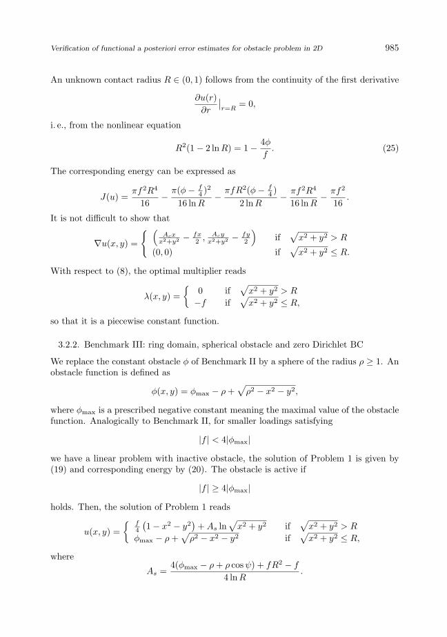
Fig. 1. Benchmark setup: Forces f pressing an elastic membrane

against a lower spherical obstacle φ. The membrane displacement

u(r) is displayed together with the contact radius R = ρ sinψ, where ρ

is a sphere radius and ψ an angular parameter.

An unknown contact radius R = ρ sinψ for some angular parameter ψ ∈ (0, arcsin 1ρ )

(see Figure 1 for details) follows from the condition of continuity of the first derivative

∂u(r)∂r

∣∣r=R

= − tanψ,

i. e., from the solution of the nonlinear equation

4(φmax − ρ+ ρ cosψ) + fρ2 sin2 ψ − f

4ρ sinψ ln(ρ sinψ)− fρ sinψ

2= − tanψ. (26)

The corresponding energy (2) can be decomposed as

J(u) = J1(u) + J2(u),

where the first term related to the contact domain Ωu =

(x, y) ∈ R2 : x2 + y2 ≤ R

reads

J1(u) =12

∫Ωu

x2 + y2

ρ2 − x2 − y2dx−

∫Ωu

f(φ− ρ+

√ρ2 − x2 − y2

)dx


and the second term related to the remaining part Ωu0 := Ω \Ωu

reads

J2(u) =12

∫Ωu

0

[A2

s

x2 + y2−Asf +

f2

4(x2 + y2

)]dx

−∫

Ωu0

[f2

4(1− x2 − y2

)+Asf ln

√x2 + y2

]dx.

Both terms can be further expressed as

J1(u) = −πρ2

2[sin2 ψ + ln(cos2 ψ)]− πfρ2(φ− ρ) sin2 ψ − 2πfρ3

3

(1−

√(1− sin2 ψ)3

),

J2(u) = −πA2s lnR− πf(2As − 1)(1−R2)

4− AsπfR

2(1− 2 lnR)2

+3πf2(1−R4)

16.


∇u(x, y) =

(

Asxx2+y2 − fx

2 ,Asy

x2+y2 − fy2

)if

√x2 + y2 > R(

− x√ρ2−x2−y2

,− y√ρ2−x2−y2

)if

√x2 + y2 ≤ R.


λ(x, y) =

0 if

√x2 + y2 > R

2ρ2−x2−y2

(ρ2−x2−y2)32− f if

√x2 + y2 ≤ R.

Remark 3.1. Existence of the first continuous derivatives ∂u(r)∂r

∣∣r=R

resulting in con-ditions (25) and (26) to determine the contact radius R can be justified by Remark2.2.

4. DISCRETIZATION AND NUMERICAL RESULTS

We verify the energy estimate (10) and the majorant estimate (12) on three aboveintroduced benchmarks. Numerical experiments are based on an own implementationof the finite element method in two dimensions. A MATLAB code is available fordownload as a package Obstacle problem in 2D and its a posteriori error estimate atMatlab Central under http://www.mathworks.com/matlabcentral/fileexchange/authors/

37756. The implementation is based on vectorization techniques of [19] and works fasteven for finer rectangular meshes.

4.1. Discretization by the finite element method

The following discretizations are considered:

• the solution v ∈ V0 of the obstacle problem is discretized in the finite dimensionalsubspace of bilinear nodal basis functions V0,h satisfying homogeneous Dirichletboundary conditions,

http://www.mathworks.com/matlabcentral/fileexchange/authors/37756

http://www.mathworks.com/matlabcentral/fileexchange/authors/37756


• the flux τ∗ ∈ H(Ω,div) of the majorant minimization problem is discretized in thefinite dimensional subspace Qh of the lowest order edge Raviart–Thomas functions,

• the Lagrange multiplier µ ∈ Λ of the majorant minimization problem is discretizedin the finite dimensional subspace Λh of the elementwise constant functions.

Let us provide more implementation details. The discrete approximation v ∈ V0,h of thesolution u of Problem 1 is expressed by a linear combination

v =N∑

j=1

vjψj

of nodal bilinear functions ψj , where N denotes a number of nodes of a consideredrectangulation T . Nodal components are assembled in a nodal (column) vector

v = (v1, . . . , vN )T .

Let us assume that N −ND internal nodes are ordered first and ND boundary Dirichletnodes last. Then, v solves a quadratic minimization problem

v = argminwi≥φi,wj=uj

12wT KBILw − bT w

, (27)

for i ∈ 1, . . . , N − ND and j ∈ N − ND + 1, . . . , N. Here φi and uj denote nodalobstacle values and nodal Dirichlet boundary values. A stiffness matrix KBIL ∈ RN×N

and a discretized loading (column) vector b = (b1, . . . , bN )T ∈ RN are constructedelemementwise as

(KBIL)ij =∫

Ω

∇ψi · ∇ψj dx, bi =∫

Ω

fψi dx (28)

for i, j ∈ 1, . . . , N. In all quadratures related to f function, f is replaced by a piecewiseconstant function f computed as the average of four nodal values on a rectangle. Weapply the built-in Matlab function quadprog to solve (27).

A discretized version of Algorithm 1 is applied for the minimization of the functionalmajorant. The minimal flux argument τ∗k+1 ∈ Qh in step (i) of Algorithm 1 is expressedby a linear combination

τ∗k+1 =M∑

j=1

yjηj ,

of edge Raviart–Thomas vector functions ηj , where M denotes a number of rectangula-tion edges. The coefficient (column) vector

y = (y1, . . . , yM )T

solves (see (14)) a linear system of equations[(1 + βk)MRT0 +

(1 +

1βk

)KRT0

]y = (1 + βk)c−

(1 +

1βk

)d. (29)


Here, a stiffness matrix KRT0 ∈ RM×M and a mass matrix MRT0 ∈ RM×M are con-structed as

(KRT0)ij =∫

Ω

divηi divηj dx, (MRT0)ij =∫

Ω

ηi · ηj dx

for i, j ∈ 1, . . . ,M and c = (c1, . . . , cM )T ∈ RM and d = (d1, . . . , dM )T ∈ RM are(column) vectors constructed as

ci =∫

Ω

∇v · ηidx, di =∫

Ω

(f + µk)divηi dx

for i ∈ 1, . . . ,M. No boundary conditions are imposed on y in (29) since the discretesolution v satisfies Dirichlet boundary conditions only. The minimal argument µk+1 ∈Λh in step (ii) of Algorithm 1 is computed locally on every rectangle from the formula

µk+1 =

−div τ∗k+1 − f − v − φ

C2Ω

(1 + 1

βk

)+

, (30)

where v, φ represent averaged rectangular values computed as the average of four nodalvalues on a rectangle and [·]+ = max0, · denotes the maximum operator.

Remark 4.1. Exact forms of local finite element matrices are reported in Appendix.

Lemma 4.2. (Discrete convergence of the majorant minimization algorithm) Let v ∈V0,h such that v 6= 0. Then, the Algorithm 1 generates a converging sequence of majorantvalues

M(v, f, φ;βk, µk, τ∗k )∞k=0

and there exists majorant parameters τ∗lim ∈ Qh, µlim ∈ Λh and βlim ≥ 0 such that

M(v, f, φ;βk, µk, τ∗k ) →M(v, f, φ;βlim, µlim, τ

∗lim) as k →∞.

P r o o f . For any nonzero function v ∈ V0,h, there is always a strictly positive distanceof ∇v to the space Qh in Ω-norm. In particular, it holds

‖∇v − τ∗k‖Ω > 0 (31)

and all iterations βk given by (16) are correctly defined.Algorithm 1 generates a nonincreasing sequence of nonnegative majorant values and

thereforeM(v, f, φ;βk, µk, τ

∗k ) →Mlim as k →∞. (32)

Consequently, the nonnegative majorant terms

M1(v, f, φ;βk, µk, τ∗k ) =

1 + βk

2‖∇v − τ∗k‖2Ω (33)

M2(v, f, φ;βk, µk, τ∗k ) =

12

(1 +

1βk

)C2

Ω‖div τ∗k + f + µk‖2Ω (34)


are bounded. Then, the boundedness of the sequence τ∗k in Ω-norm follows from theboundedness of the first majorant term (33). Since Qh is finite-dimensional, the sequenceτ∗k has a converging subsequence τ∗km

denoted as τ∗m and

τ∗m → τ∗lim as m→∞,

div τ∗m → div τ∗lim as m→∞.

The boundedness of the sequence µm in Ω-norm follows from the boundedness of thesecond majorant term (34). Since Λh is finite-dimensional, the sequence µm has aconverging subsequence µml

denoted as µl and

µl → µlim ∈ Λh as l→∞.

Since ‖∇v−τ∗l ‖Ω → ‖∇v−τ∗lim‖Ω > 0 and ‖div τ∗l +f+µl‖Ω → ‖div τ∗lim+f+µlim‖Ω ≥ 0as l→∞, it follows from (16) that

βl → βlim =‖div τ∗lim + f + µlim‖Ω

‖∇v − τ∗lim‖Ω< +∞ as l→∞.

Finally, it follows from continuity of the majorant (13) that

M(v, f, φ;βl, µl, τ∗l ) →M(v, f, φ;βlim, µlim, τ

∗lim) as l→∞ (35)

and (32) and (35) implies

Mlim = M(v, f, φ;βlim, µlim, τ∗lim).

Remark 4.3. The formulation of Lemma 4.2 still admits that

(τ∗lim, µlim, βlim) 6= argminτ∗∈Qh,µ∈Λh,β>0

M(v, f, φ;β, µ, τ∗)

and therefore it only holds

M(v, f, φ;βlim, µlim, τ∗lim) ≥ min

τ∗∈Qh,µ∈Λh,β>0M(v, f, φ;β, µ, τ∗).

Remark 4.4. In all numerical experiments, only two iterations of Algorithm 1 wereapplied in which we set β0 = 1 and µ0 is provided from the quadratic programmingfunction quadprog. Without a good initial iteration µ0, the number of iterations wouldbe significantly higher as already demonstrated in 1D numerical experiments [13].

Remark 4.5. In the particular case v = 0, Lemma 4.2 does not state the convergenceof Algorithm 1. If τ∗k+1 = 0 additionally, it holds

‖∇v − τ∗k‖Ω = 0

and the exact analysis shows:


• µk+1 is computed in step (ii) from (30) as µk+1 =[−f + φ

C2Ω

“1+ 1

βk

”]+

.

• βk+1 → +∞ in step (iii).

• τ∗k+2 is computed in step (i) from the limiting linear system of equations (29) inthe form MRT0y = 0, where MRT0 is a regular matrix. Therefore, τ∗k+2 = 0.

• µk+2 is computed in step (ii) from (30) as µk+2 =[−f + φ

C2Ω

]+

.

• βk+2 → +∞ in step (iii).

Obviously Algorithm 1 converges to the limit

(τ∗lim, µlim, βlim) = (0, µk+2,+∞).

However, in practical computations, the extension of real values by the value +∞ re-quires a special attention.

Remark 4.6. Generally, 0 ≤ βk <∞ in Algorithm 1 and therefore

0 ≤ βlim <∞.

If βk = 0, then the second majorant term (34) is replaced by its limit

M2(v, f, φ;βk, µk, τ∗k ) → 0 as βk → 0+

in the implementation.

4.2. Verification of error estimates

We verify the energy estimate (10) and the majorant estimate (12) for all three in-troduced benchmarks discretized on uniform rectangular meshes Th generated by theuniform mesh parameter

h ∈

12,14,18,

116,

132,

164

.

The (squared) error is approximately evaluated by a quadratic form

‖vh − u‖2E ≈ (vh − uh)T KBILh (vh − uh) (36)

using a discrete solution vector vh, a nodal interpolation vector uh of the exact solutionu and a stiffness matrix matrix KBIL

h on a considered mesh Th. The error value isfurther improved by evaluations of quadratic forms

‖vh − u‖2E ≈ (Ph/2(vh)− uh/2)T KBILh/2 (Ph/2(vh)− uh/2) (37)

or‖vh − u‖2E ≈ (Ph/4(vh)− uh/4)T KBIL

h/4 (Ph/4(vh)− uh/4) (38)


using nodal prolongation matrices Ph/2 and Ph/4 from Th to once and twice uniformlyrefined rectangular meshes Th/2 and Th/4 and nodal interpolations vectors uh/2 and uh/4

of the exact solution u on Th/2 and Th/4. Postprocessing of (37), (38) requires extramemory resources but proves important to keep a proper inequality sign in the energyestimate (10). The value of (38) is used in all convergence figures and all values (36),(37), (38) are prompted in the code run for comparison.

In Benchmark I, we consider the contact radius

R = 0.7

only. The finest meshes are Th=1/64 to provide the discrete solution vh and Th=1/256 toevaluate its error ‖vh − u‖E according to (38) are characterized by mesh properties

Th=1/64 : 16384 elements, 16641 nodes and 33024 edges

Th=1/256 : 262144 elements, 263169 nodes and 525312 edges.

Figures 2 and 3 display the discrete solution, a discrete flux component in x-direction anda discrete multiplier computed from the majorant minimization algorithm (Algorithm1) on the rectangular mesh Th=1/16. This mesh is not the finest mesh available butit is coarse enough to stress out the shape of applied finite elements. A discrete fluxcomponent in y-direction is not shown due to symmetry reasons. Local distributionsof the exact error and of the functional majorant are compared in Figure 4. Localdistributions of majorant parts are depicted in Figure 5. The amplitude of the firstmajorant part

‖∇v − τ∗‖2Ω (39)

is significantly higher than amplitudes of the equilibrium and nonlinear parts ‖div τ∗ +f + µ‖2Ω and

∫Ωµ(v − φ)dx. The nonlinear part indicates a layer of elements located

around a boundary of the contact domain corresponding to the discrete solution v.Converge behavior for all considered rectangulations is compared in Figure 6. We cansee that the energy estimate (10) and the majorant estimate (12) are very sharp withvalid inequalities signs.

Remark 4.7. A simplified least-square (LS) variant of the function majorant type es-timate was tested on the same benchmark including a mesh adaptivity in [7]. The maindifference is that nonlinear term

∫Ωµ(v − φ)dx is considered here in order to guarantee

the majorant upper bound in (12) and enhance an accurate error control.

In Benchmark II and Benchmark III, we consider the cases

f = −10, φ = −1 (for Benchmark II)

f = −10, φmax = −1, ρ = 1.2 (for Benchmark III)

only. Numerical solutions of (25) and (26) show that contact radius R is approxi-mately R ≈ 0.5024744 for Benchmark II and R ≈ 0.4389205 for Benchmark III. Sinceour implementation runs on rectangular elements allowing a polygonal boundary only,


Fig. 2. Discrete solution v of the obstacle problem and the lower

obstacle φ (left) and its rotated view (right). The dark blue color

indicates the contact domain.

Fig. 3. Discrete flux x-component τ∗x (top left) and discrete

multiplier µ (bottom left) of the majorant minimization and exact flux

x-component ∂u∂x

(top right) and exact multiplier λ (bottom right).


Fig. 4. Local distribution of the exact error 12‖v − u‖2E (left) and of

the functional majorant M(v, . . . ) (right).

Fig. 5. Local distributions of the functional majorant parts:

‖∇v − τ∗‖2Ω (top), ‖div τ∗ + f + µ‖2Ω (left bottom),RΩµ(v − φ)dx

(right bottom). Note that the part ‖∇v − τ∗‖2Ω contributes mostly to

the functional majorant.


Fig. 6. Benchmark on a square domain with a constant obstacle:

convergence.

Fig. 7. Rectangulation of the ring domain. The green line indicates

the exact ring boundary, red rectangles are completely inscribed in

the ring boundary and blue circumscribed rectangles contain at least

one node lying outside the ring boundary. Red rectangles define an

inscribed rectangulation T∨ and red and blue rectangles together

define a circumscribed rectangulation T ∧.


we consider an inscribed rectangulation T∨ and a circumscribed rectangulation T ∧ asapproximations of the ring boundary, see Figure 7 for details.

A discrete solution v∨ is solved on T∨ satisfying zero Dirichlet boundary conditionson its boundary ∂T∨. Then, v∨ is extended by zero values on T ∧ \ T∨ (displayed by theblue color rectangles in Figure 7) to define a discrete solution v∧ on the circumscribedrectangulations T ∧. It can be easily checked that

J(v∨) :=12

∫T∨∇v∨·∇v∨ dx−

∫T∨f∨v∨ dx =

12

∫T ∧

∇v∧·∇v∧ dx−∫T ∧

f∧v∧ dx := J(v∧),

where f∨ represents a restriction of f to T∨ and f∧ represents an extension of f∨ toT ∧ \ T∨ by any value. The extension f∧ is defined by the same constant function f inour implementation. Finally, the majorant minimization is computed on T ∧. Thus themodification of the energy estimate (10) and the majorant estimate (12) is combined inthe estimate

12

∣∣∣∣v∨ − u|T∨∣∣∣∣2

E≤ J(v∧)− J(u) ≤M(v∧, f∧, φ∧;β, µ∧, τ∗∧), (40)

which is shown in convergence figures. Figures 8 and 10 display discrete solutions v ofBenchmark II and Benchmark III computed on rectangulation created for h = 1

16 andFigures 9 and 11 a discrete flux component in x-direction τx and a discrete multiplier µcomputed from the majorant minimization algorithm (Algorithm 1) on the same rectan-gulation. Converge behaviour for all considered rectangulations is compared in Figures12 and 13. We can see that the modified energy and majorant estimates (40) are sharp.

CONCLUSIONS

Computations for discussed benchmarks with known analytical solutions demonstratethat the functional majorant serves as a fully computable tool to estimate the upperbound of the difference of energies J(v)− J(u) which serves further as an upper boundof the error in the energy norm. The majorant minimization algorithm consists of thesolution of a linear system of equations for a flux variable and elementwise computationof the Lagrange multiplier. If a good a initial Lagrange multiplier field is availabletogether with the discrete solution of the obstacle problem, the majorant minimizationalgorithm requires only few iterations to provide a sharp upper bound of the error.

APPENDIX — LOCAL FEM MATRICES

We assume a reference rectangle Tref with lengths hx and hy specified by vertices

v1 = (0, 0), v2 = (0, hx), v3 = (hx, hy), v4 = (0, hy)

and define four local bilinear nodal basic functions

ψ1(x, y) = 1− y

hy− x

hx+

xy

hxhy, ψ2(x, y) =

x

hx− xy

hxhy,

ψ3(x, y) =xy

hxhy, ψ4(x, y) =

y

hy− xy

hxhy


Fig. 12. Benchmark on a ring domain with a constant obstacle:

convergence.

Fig. 13. Benchmark on a ring domain with a spherical obstacle:

convergence.


satisfying the relation ψi(vj) = δij for i, j = 1, . . . 4. Corresponding gradients

∇ψ1(x, y) =(− 1hx

+y

hxhy, − 1

hy+

x

hxhy

),

∇ψ2(x, y) =(

1hx

− y

hxhy, − x

hxhy

),

∇ψ3(x, y) =(

y

hxhy,

x

hxhy

),

∇ψ4(x, y) =(− y

hxhy,

1hy

− x

hxhy

)are linear functions. Local stiffness matrix is defined as

(KBILref )ij =

∫Tref

∇ψi · ∇ψj dx

and direct computation shows

KBILref =

16hxhy

2h2

x + 2h2y h2

x − 2h2y −h2

x − h2y −2h2

x + h2y

h2x − 2h2

y 2h2x + 2h2

y −2h2x + h2

y −h2x − h2

y

−h2x − h2

y −2h2x + h2

y 2h2x + 2h2

y h2x − 2h2

y

−2h2x + h2

y −h2x − h2

y h2x − 2h2

y 2h2x + 2h2

y

.

Local Raviart–Thomas basis functions (of the lowest order) are vector edge based basisfunctions

η1(x, y) :=(0 , 1− y

hy

), η2(x, y) :=

( x

hx, 0

),

η3(x, y) :=(0 ,

y

hy

), η4(x, y) :=

(1− x

hx, 0

)defined on reference edges

e1 = v1, v2, e2 = v2, v3, e3 = v3, v4, e4 = v4, v1

and they satisfy the relation ηi|ej·nj = δij , where global normals nj related to edges ej

are always oriented in directions of the coordinate system,

n1 = (0, 1), n2 = (1, 0), n3 = (0, 1), n4 = (1, 0).

This choice of global normals leads to a simpler implementation with no issues relatedto global orientation of edges. The corresponding divergences

div η1 = − 1hy, div η2 =

1hx, div η3 =

1hy, div η4 = − 1

hx

are constant functions. Local stiffness and mass matrices defined by relations

(KRT0ref )ij =

∫Tref

divηi divηj dx, (MRT0ref )ij =

∫Tref

ηi · ηj dx


read

KRT0ref =

hx

hy−1 −hx

hy1

−1 hy

hx1 −hy

hx

−hx

hy1 hx

hy−1

1 −hy

hx−1 hy

hx

, MRT0ref = hxhy

13 0 1

6 00 1

3 0 16

16 0 1

3 00 1

6 0 13

.

ACKNOWLEDGMENT

The first author was supported by the project CZ.1.07/2.3.00/30.0039 Excellent young re-searcher at Brno University of Technology. The second author acknowledges the support of theproject GA13-18652S (GA CR).

(Received August 4, 2014)

R E FER E NCE S

[1] M. Ainsworth and J.T. Oden: A Posteriori Error Estimation in Finite Element Analysis.Wiley and Sons, New York 2000.

[2] I. Babuska and T. Strouboulis: The finite Element Method and its Reliability. OxfordUniversity Press, New York 2001.

[3] W. Bangerth and R. Rannacher: Adaptive Finite Element Methods for DifferentialEquations. Birkhauser, Berlin 2003.

[4] D. Braess, R.H. W. Hoppe, and J. Schoberl: A posteriori estimators for obstacle problemsby the hypercircle method. Comput. Vis. Sci. 11 (2008), 351–362.

[5] F. Brezi, W. W. Hager, and P. A. Raviart: Error estimates for the finite element solutionof variational inequalities I. Numer. Math. 28 (1977), 431–443.

[6] H. Buss and S. Repin: A posteriori error estimates for boundary value problems withobstacles. In: Proc. 3nd European Conference on Numerical Mathematics and AdvancedApplications, Jyvaskyla 1999, World Scientific 2000, pp. 162–170.

[7] C. Carstensen and C. Merdon: A posteriori error estimator competition for conformingobstacle problems. Numer. Methods Partial Differential Equations 29 (2013), 667–692.

[8] Z. Dostal: Optimal Quadratic Programming Algorithms. Springer 2009.

[9] R. S. Falk: Error estimates for the approximation of a class of variational inequalities.Math. Comput. 28 (1974), 963–971.

[10] M. Fuchs and S. Repin: A posteriori error estimates for the approximations of the stressesin the Hencky plasticity problem. Numer. Funct. Anal. Optim. 32 (2011), 610–640.

[11] R. Glowinski, J. L. Lions, and R. Tremolieres: Numerical Analysis of Variational Inequal-ities. North-Holland 1981.

[12] B. Gustafsson: A simple proof of the regularity theorem for the variational inequality ofthe obstacle problem. Nonlinear Anal. 10 (1986), 12, 1487–1490.

[13] P. Harasim AD J. Valdman: Verification of functional a posteriori error estimates forobstacle problem in 1D. Kybernetika 49 (2013), 5, 738–754.

[14] I. Hlavacek, J. Haslinger, J. Necas, and J. Lovısek: Solution of variational inequalities inmechanics. Applied Mathematical Sciences 66, Springer-Verlag, New York 1988.


[15] D. Kinderlehrer and G. Stampacchia: An Introduction to Variational Inequalities andTheir Applications. Academic Press, New York 1980.

[16] J. L. Lions and G. Stampacchia: Variational inequalities. Comm. Pure Appl. Math. 20(1967), 493–519.

[17] P. Neittaanmaki and S. Repin: Reliable Methods for Computer Simulation (Error Controland A Posteriori Estimates). Elsevier, 2004.

[18] R. H. Nochetto, K. G. Seibert, and A. Veeser: Pointwise a posteriori error control forelliptic obstacle problems. Numer. Math. 95 (2003), 631–658.

[19] T. Rahman and J. Valdman: Fast MATLAB assembly of FEM matrices in 2D and 3D:nodal elements. Appl. Math. Comput. 219 (2013), 7151–7158.

[20] S. Repin: A posteriori error estimation for variational problems with uniformly convexfunctionals. Math. Comput. 69 (230) (2000), 481–500.

[21] S. Repin: A posteriori error estimation for nonlinear variational problems by dualitytheory. Zapiski Nauchn. Semin. POMI 243 (1997), 201–214.

[22] S. Repin: Estimates of deviations from exact solutions of elliptic variational inequalities.Zapiski Nauchn. Semin, POMI 271 (2000), 188–203.

[23] S. Repin: A Posteriori Estimates for Partial Differential Equations. Walter de Gruyter,Berlin 2008.

[24] S. Repin and J. Valdman: Functional a posteriori error estimates for problems withnonlinear boundary conditions. J. Numer. Math. 16 (2008), 1, 51–81.

[25] S. Repin and J. Valdman: Functional a posteriori error estimates for incremental modelsin elasto-plasticity. Centr. Eur. J. Math. 7 (2009), 3, 506–519.

[26] M. Ulbrich: Semismooth Newton Methods for Variational Inequalities and ConstrainedOptimization Problems in Function Spaces. SIAM, 2011.

[27] J. Valdman: Minimization of functional majorant in a posteriori error analysis based onH(div) multigrid-preconditioned CG method. Adv. Numer. Anal. (2009).

[28] Q. Zou, A. Veeser, R. Kornhuber, and C. Graser: Hierarchical error estimates for theenergy functional in obstacle problems. Numer. Math. 117 (2012), 4, 653–677.

Petr Harasim, Brno University of Technology, Faculty of Civil Engineering, Veverı 95,602 00 Brno. Czech Republic.

e-mail: [email protected]

Jan Valdman, Institute of Mathematics and Biomathematics, Faculty of Science, Uni-versity of South Bohemia, Branisovska 31, 370 05 Ceske Budejovice and Institute ofInformation Theory and Automation — Academy of Sciences of the Czech Republic,Pod Vodarenskou vezı 4, 182 08 Praha 8. Czech Republic.

e-mail: [email protected]

Hava14 article

Documents

Transcript of Hava14 article