Interpolation schemes in the displaced-diffusion libor market
40
INTERPOLATION SCHEMES IN THE DISPLACED-DIFFUSION LIBOR MARKET MODEL AND THE EFFICIENT COMPUTATION OF PRICES AND GREEKS FOR CALLABLE RANGE ACCRUALS CHRISTOPHER BEVERIDGE AND MARK JOSHI A. We introduce a new arbitrage-free interpolation scheme for the displaced-diffusion LIBOR market model. Using this new extension, and the Piterbarg interpolation scheme, we study the simulation of range accrual coupons when valuing callable range accruals in the displaced- diffusion LIBOR market model. We introduce a number of new improvements that lead to significant efficiency improvements, and explain how to apply the adjoint-improved pathwise method to calculate deltas and vegas under the new improvements, which was not previously possible for callable range accruals. One new improvement is based on using a Brownian-bridge-type approach to simulating the range accrual coupons. We consider a variety of examples, including when the reference rate is a LIBOR rate, when it is a spread between swap rates, and when the multiplier for the range accrual coupon is stochastic. 1. I An exotic interest rate derivative which has become very popular is the callable range accrual or floating range note. For such a product, the size of each coupon depends on the number of days during the accrual period where a reference rate is within a pre-specified range. The reference rate is commonly a LIBOR rate, but can also be a swap rate or the spread between two interest rates. As such, the coupon payments are made up of a number of individual digital options. While callable range accruals are very popular, the accurate pricing and efficient Greek calculations of these products provide a number of challenges, which have not been fully overcome. In particular, we need to observe the yield curve on a daily basis to determine the pay-off, we need to cope with Bermudan optionality and we want to be able to calibrate to a large number of hedging instruments. In addition, the discontinuous nature of the coupons makes computing sensitivities tricky. The displaced diffusion LIBOR market model (DDLMM) is a standard approach to pricing exotic interest rate derivatives with the virtue that it can be calibrated to large numbers of market instruments, and can also achieve skew. See, for example, [1]. However, the Bermudan optionality, the discontinuities and daily observations make it challenging to apply to this problem. Our objective in this paper is to develop extensions to the DDLMM that allow the prices and Greeks of callable range accrual notes to be computed in a similar fashion and with similar speed to other exotic interest rate derivatives. We introduce a number of innovations and apply our recent results on pricing breakable contracts by Monte Carlo, [5]. In order to avoid evolving thousands of rates, it is necessary to use an interpolation scheme that allows the deduction of non-tenor rates within a simulation. Whilst schemes have previously been suggested by Piterbarg [22] and Schlögl [24], we will see that if one wishes the scheme to have no internal arbitrages, have stochastic rates at all times before reset and have rates that remain positive (when displacements are zero), it is necessary to introduce a new scheme. We introduce such a scheme and show how the values of rates within it can be approximately computed. 1
-
Upload
khangminh22 -
Category
Documents
-
view
8 -
download
0
Transcript of Interpolation schemes in the displaced-diffusion libor market

INTERPOLATION SCHEMES IN THE DISPLACED-DIFFUSION LIBOR MARKETMODEL AND THE EFFICIENT COMPUTATION OF PRICES AND GREEKS FOR
CALLABLE RANGE ACCRUALS
CHRISTOPHER BEVERIDGE AND MARK JOSHI
Abstract. We introduce a new arbitrage-free interpolation scheme for the displaced-diffusionLIBOR market model. Using this new extension, and the Piterbarg interpolation scheme, we studythe simulation of range accrual coupons when valuing callable range accruals in the displaced-diffusion LIBOR market model. We introduce a number of new improvements that lead to significantefficiency improvements, and explain how to apply the adjoint-improved pathwise method to calculatedeltas and vegas under the new improvements, which was not previously possible for callable rangeaccruals. One new improvement is based on using a Brownian-bridge-type approach to simulatingthe range accrual coupons. We consider a variety of examples, including when the reference rateis a LIBOR rate, when it is a spread between swap rates, and when the multiplier for the rangeaccrual coupon is stochastic.
1. Introduction
An exotic interest rate derivative which has become very popular is the callable range accrualor floating range note. For such a product, the size of each coupon depends on the number of daysduring the accrual period where a reference rate is within a pre-specified range. The referencerate is commonly a LIBOR rate, but can also be a swap rate or the spread between two interestrates. As such, the coupon payments are made up of a number of individual digital options.While callable range accruals are very popular, the accurate pricing and efficient Greek
calculations of these products provide a number of challenges, which have not been fully overcome.In particular, we need to observe the yield curve on a daily basis to determine the pay-off, weneed to cope with Bermudan optionality and we want to be able to calibrate to a large numberof hedging instruments. In addition, the discontinuous nature of the coupons makes computingsensitivities tricky.The displaced diffusion LIBOR market model (DDLMM) is a standard approach to pricing
exotic interest rate derivatives with the virtue that it can be calibrated to large numbers of marketinstruments, and can also achieve skew. See, for example, [1]. However, the Bermudan optionality,the discontinuities and daily observations make it challenging to apply to this problem.
Our objective in this paper is to develop extensions to the DDLMM that allow the prices andGreeks of callable range accrual notes to be computed in a similar fashion and with similar speedto other exotic interest rate derivatives. We introduce a number of innovations and apply ourrecent results on pricing breakable contracts by Monte Carlo, [5].
In order to avoid evolving thousands of rates, it is necessary to use an interpolation scheme thatallows the deduction of non-tenor rates within a simulation. Whilst schemes have previously beensuggested by Piterbarg [22] and Schlögl [24], we will see that if one wishes the scheme to haveno internal arbitrages, have stochastic rates at all times before reset and have rates that remainpositive (when displacements are zero), it is necessary to introduce a new scheme. We introducesuch a scheme and show how the values of rates within it can be approximately computed.
1

2 CHRISTOPHER BEVERIDGE AND MARK JOSHI
In order to avoid evolution to every observation date which would be very slow, we employ twodevices. The first is to clump observations together. We will see that provided the clumping is donesymmetrically, it is very accurate. The second is to compute expectations of the accrual couponsconditional on the values of rates during the simulation. We will, in fact, do so in two differentways. For the first, we compute conditional expectations at the start of accrual period. For thesecond, we also condition on the values of rates at the end of the accrual period. This Brownianbridging approach has the additional virtue that floating coupons are easy to value, and that thesizes of approximation errors are reduced. Since both methods replace discontinuous coupons byexpectations which are smooth functions of their parameters, they allow the application of thepathwise method for computing Greeks. See [23] or [11].
We will show that our techniques are effective for a variety of callable range accrual contracts;in particular, we will study the cases when the reference rate is a LIBOR rates and when it is adifference of two swap-rates. We will also allow the coupon to be determined by a floating rate inarrears.
The structure of the paper is as follows. In Section 2 we briefly recap the DDLMM. In Section3 we provide some additional notation and introduce our main examples. Various interpolationmethodologies are introduced in Section 4 and justified. In Section 5, we show how the simulationcan be effectively implemented, and in Section 6 we provide numerical results. These demonstratesignificant efficiency improvements for both prices and Greeks.
2. The Displaced-Diffusion LIBOR Market Model
Since it was given a firm theoretical base in the fundamental papers by Brace, Gatarek andMusiela, [7], Musiela and Rutkowski, [21], and Jamshidian, [15], the LIBOR market model hasbecome a very popular method for pricing exotic interest rate derivatives. It is based on the ideaof evolving the yield curve directly through a set of discrete market observable forward rates,rather than indirectly through use of a single non-observable quantity which is assumed to drivethe yield curve. A distinct advantage of this approach is the ability to easily calibrate to a largenumber of simpler financial contracts, often used in the hedging process for exotics; see [1].Suppose we have a set of tenor dates, 0 = T0 < T1 < . . . < Tn+1. Let δj = Tj+1 − Tj , and let
P (t, T ) denote the price at time t of a zero-coupon bond paying one at its maturity, T . For easeof exposition, we will assume throughout that δj = δ is constant for all j. Let L(t, T ) denote thevalue of the forward rate from T to T + δ as of time t. Using no-arbitrage arguments,
L(t, T ) =
P (t,T )P (t,T+δ)
− 1
δ,
where L(t, T ) is said to reset at time T , after which point it is assumed that it does not change invalue. To simplify notation, let
Lj(t) = L(t, Tj) and Pj(t) = P (t, Tj).
We work in the spot LIBOR measure, which corresponds to using the discretely-compoundedmoney market account as numeraire, because this has certain practical advantages; see [16]. Thisnumeraire is made up of an initial portfolio of one zero-coupon bond expiring at time T1, with theproceeds received when each bond expires being reinvested in bonds expiring at the next tenordate, up until Tn+1. More formally, the value of the numeraire portfolio at time t will be,
N(t) = P (t, Tη(t))
η(t)−1∏i=1
(1 + δLi(Ti)),

INTERPOLATION SCHEMES AND CALLABLE RANGE ACCRUALS IN THE DDLMM 3
where η(t) is the unique integer satisfying
Tη(t)−1 ≤ t < Tη(t),
and thus gives the index of the next forward rate to reset.Under the DDLMM, the forward rates that make up the state variables of the model are assumed
to be driven by the following process
dLi(t) = µi(L(t), t)(Li(t) + αi)dt+ σi(t)(Li(t) + αi)dWi(t), (2.1)
where the σi(t)’s are deterministic functions of time, the αi’s are constant displacement coefficients,the Wi’s are standard Brownian motions under the spot LIBOR martingale measure, L(t) denotesthe vector of state variables at time t, and the µ′is are uniquely determined by no-arbitragerequirements. It is assumed that Wi and Wj have correlation ρi,j , and throughout {Ft}t≥0 willbe used to denote the filtration generated by the driving Brownian motions. Primarily to easenotation, but also to maintain time-homogeneity, we assume that the displacement coefficients arethe same for all forward rates, that is
αi = α,
for all values of i. However, where it is not obvious, we will explain how to apply the techniquesdiscussed when the displacements of different forward rates are not equal. To further ease notation,let
Lj(t) = Lj(t) + α.
The requirement that the discounted price processes of the fundamental tradeable assets, thatis the zero-coupon bonds associated to each tenor date, be martingales in the pricing measure,dictates that the drift term is
µi(L(t), t) =i∑
j=η(t)
Lj(t)δ
1 + Lj(t)δσi,j(t),
see [8], whereσi,j(t) = σi(t)σj(t)ρi,j,
and therefore denotes the instantaneous covariance between the logarithms of (L(t, Ti) + α) and(L(t, Tj) + α). In addition, let Ci,j(s, t) denote the integral of σi,j(.) over the interval (s, t). Ift < s we make the convention that this equals zero. We also let Vj(s, t) = Cj,j(s, t).When developing analytic approximations in the DDLMM, a useful tool is the common drift-
freezing approximation (see, for example, [8]). The idea is to freeze all state-dependence in thedrifts of (2.1) at the current time, so as to obtain a lognormal approximation to the forward rates.In particular, conditional on Fs, we have
dLi(t) ≈ µi(L(s), t)Li(t)dt+ σi(t)Li(t)dWi(t), (2.2)
for t > s. We will need this approximation at various stages later on.Displaced-diffusion is used as a simple way to allow for the skews seen in implied caplet
volatilities that have long persisted in interest rate markets; see [16]. In particular, the use ofdisplaced-diffusion allows for the wealth of results concerning calibrating and evolving rates in thestandard LIBOR market model to be carried over with only minor changes. The model presentedcollapses to the standard LIBOR market model when α = 0.

4 CHRISTOPHER BEVERIDGE AND MARK JOSHI
3. Notation and Products
We consider a swap where the issuer receives the floating LIBOR rate with a natural time-lagand pays a range accrual coupon, Si, at each tenor date Ti (for i ≥ 2), until the time of exercise.The range accrual coupon is given by
Si =Qi
ni
ni∑j=1
IBi<R(Ti−1+tj)<Ui ,
where ni denotes the number of observation days for the (i− 1)th range accrual coupon, R(t) thevalue of the underlying reference rate at time t, and Ti−1 + tj the time of the jth observation day.Note that Qi can be stochastic, whereas Bi and Ui will generally be deterministic. However, themethods introduced in this paper can easily handle the case where Bi and Ui are FTi−1
-measurable.Also note that this particular set-up has one-sided range accruals as a special case.
We consider three examples. These are chosen to represent the most common coupon structures,as well as the most difficult to handle. However, the techniques introduced can easily be appliedor extended to any similar product. In particular, we consider
• Example 1: R(t) = L(t, t), Qi = q. This is the most common coupon structure, where themultiplier, Qi, is deterministic, and the reference rate is the spot LIBOR rate, denoted byL(t, t).• Example 2: R(t) = SRt,x(t) − SRt,y(t) for x > y, Qi = q, where SRt,x(s) denotes thevalue of the swap rate starting at time t and running for x accrual periods, as of time s.As such, the reference rate is a spread between constant maturity spot swap rates.• Example 3: R(t) = SRt,x(t) − SRt,y(t) for x > y, Qi = qLi(Ti). The multiplier is nowstochastic, and is proportional to the forward rate resetting at the end of the accrualperiod. This feature, together with the reference rate, make this particular coupon structureparticularly challenging.
.For simplicity, assume that the product can be exercised on each of the tenor dates T1, . . . , Tn,
where the time of exercise is decided by the issuer. We also assume that the rebate received bythe issuer upon exercise is zero. Let τ denote a given exercise strategy taking values in the set
{1, 2, . . . , n, n+ 1},
representing the set of possible exercise times. Note that we assume an extra exercise time, indexedby n+ 1, where exercise must occur and zero rebate is received upon exercise. This is done toensure that we have a finite stopping time as an exercise strategy.For ease of exposition, let Et
T (.) = ET (.|Ft), where the subscript is used to denote that theequivalent martingale measure associated with the numeraire asset P (t, T ) is being used. If nosubscript is present, it is implicitly assumed that the equivalent martingale measure associatedwith N(t) is being used.
For brevity later on, we introduce the following notation. Let
θ(t) = Tη(t) − t and ϑ(t) = t− Tη′ (t),
withη′(t) = η(t)− 1.

INTERPOLATION SCHEMES AND CALLABLE RANGE ACCRUALS IN THE DDLMM 5
Finally, throughout we will work with the understanding that when i > k,k∏j=i
= 1 andk∑j=i
= 0.
4. Interpolation Methods
Since callable range accruals depend on non-tenor forward rates and swap rates, a method toextend the DDLMM to continuous tenor is needed. In this paper we consider two approaches. Thefirst is a simple method introduced by Piterbarg, [22], that will be briefly described in Section 4.1.For the second method, we use the more complicated, but theoretically appealing framework ofSchlögl, [24], extended to the DDLMM. We introduce a new way to apply this framework thatresults in more realistic interpolations while maintaining desirable properties for the interpolatedbond prices. The standard framework is discussed in Section 4.2 and our extension in Section 4.3.For all approaches considered, the extension to continuous tenor is carried out by interpolatingzero-coupon bond prices in the maturity dimension using the discrete tenor forward rates at thecurrent time.
In order to compare the different interpolation schemes, we study three properties:(1) Absence of internal arbitrage: arbitrage opportunities do not exist by trading with the
non-tenor bonds.(2) Positivity: if displacements are zero, that is α = 0, then interpolated forward rates are
positive. This property precludes arbitrage with cash in the standard LIBOR market model.(3) Stochasticity: P (t1, t2) is stochastic for all t1 < t2.
4.1. Piterbarg Interpolation. In order to extend the DDLMM to continuous tenor, Piterbarg,[22], assumes that the forward rates applying over periods surrounded by tenor dates are equal tothe forward rates associated with the surrounding tenor dates. As a result, the DDLMM can beextended to continuous tenor in three steps,
• P (t1, t2) = (1 + (t2 − t1)Lη′ (t1)(t1))−1, for t2 ≤ Tη(t1),• Pj(t1) = Pη(t1)(t1)
∏j−1k=η(t1)(1 + δLk(t1))−1, for j ≥ η(t1),
• P (t1, t2) = Pη′ (t2)(t1)(1 + ϑ(t2)Lη′ (t2)(t1))−1, for t2 > Tη(t1).We therefore have
Theorem 4.1. The Piterbarg interpolation scheme satisfies Positivity.
Proof. That Positivity holds is obvious from
L(t1, t2) =
1δ
[(1+θ(t1)L
η′(t1)
(t1))(1+ϑ(t2+δ)Lη(t1)(t1))
1+(t2−t1)Lη′(t1)
(t1)− 1
], if t2 < Tη(t1);
1δ
[(1+δL
η′(t2)
(t1))(1+ϑ(t2+δ)Lη(t2)(t1))
1+ϑ(t2)Lη′(t2)
(t1)− 1
], otherwise,
since the leading term of the numerator in each fraction is at least as big as the denominator andthe second term of the numerator in each fraction is greater than 1. �
It is clear that Stochasticity fails under the Piterbarg interpolation scheme from the definitionof P (t1, t2) for t2 ≤ Tη(t1), and we demonstrate that the scheme is internally arbitrageable withthe following example.

6 CHRISTOPHER BEVERIDGE AND MARK JOSHI
Suppose we are at time t and t < t1 < t2 < Tη(t), then we can construct two portfolios whichalways have the same value at t1, but have different initial values. The first portfolio is made upon one unit of P (t, t2). In contrast, the second portfolio is made up of
P (t1, t2) =1
1 + (t2 − t1)Lη′ (t)(Tη′ (t))
units of P (t, t1). The second portfolio is then worth less at time t since
P (t1, t2)P (t, t1) < P (t, t2),
and both portfolios are worth P (t1, t2) at t1.
4.2. Schlögl Interpolation. We can use the interpolation framework introduced in [24] to extendthe DDLMM to continuous tenor in a way that precludes arbitrage and is consistent with theassumptions of the DDLMM. While the framework from [24] is used, we introduce a new way toapply it. This is required to maintain a sufficient level of volatility in the interpolated bond prices,while providing a realistic interpolation scheme that precludes arbitrage with cash. In doing so,we also extend Schlögl’s framework from the LIBOR market model to the DDLMM.
First, consider the framework in [24]. Define the short bond at a given time to be the zero-couponbond maturing on the next tenor date. Under the assumptions of the DDLMM, we have the uniqueprocesses for the ratios of zero-coupon bond prices under each equivalent martingale measure. Anychoice of processes for the absolute zero coupon bond prices that are consistent with these willtherefore not introduce arbitrage amongst the zero-coupon bonds by construction, although somechoices may imply unrealistic dynamics that lead to arbitrage opportunities outside the model. Ifan interpolation method is specified for the short bonds at all times, then the processes for thezero-coupon bonds that are consistent with the DDLMM are completely and uniquely determined.As such, we can specify any interpolation method we want for the short bonds at all times,without introducing internal arbitrage and maintaining consistency with the assumptions of theDDLMM. Once this is done, the continuous tenor model is completely specified by no-arbitragerequirements. In particular, the unique arbitrage-free price for an arbitrary zero-coupon bond atany time, P (t1, t2) (where t1 < t2 < Tn+1), is given by
P (t1, t2)
Pη(t2)(t1)= Et1
Tη(t2)
[1
Pη(t2)(t2)
], (4.1)
where the values of Pη(t2)(t2) and Pη(t2)(t1) are determined by the specified method for interpolatingshort bonds, and thus so is the P (t1, t2). Applying the arbitrage-free interpolation scheme of [24]then reduces to specifying how the short bonds are interpolated at all times.
In [24], an interpolation method for the short-bonds that allows for volatility in their prices isgiven. Schlögl assumed that
Pη(t1)(t1)−1 = 1 + θ(t1)[ξ(t1)Lη′ (t1)(Tη′ (t1)) + (1− ξ(t1))Lη(t1)(t1)
], (4.2)
for some user-specified function ξ(t) that satisfies
lim∆↘0
ξ(Ti + ∆) = 1, (4.3)
lim∆↗Ti+1−Ti
ξ(Ti + ∆) = 0, (4.4)
for all i = 0, 1, . . . , n. Note that ξ(t) can be used to control the level of volatility in the shortbonds; the smaller ξ(t) is, the greater the dependence on Lη(t1)(t1) in (4.2), and the greater the

INTERPOLATION SCHEMES AND CALLABLE RANGE ACCRUALS IN THE DDLMM 7
volatility in Pη(t1)(t1). In addition, due to the flexibility in ξ(t), in effect (4.2) specifies a familyof assumptions.
Using this assumption in (4.1) givesP (t1, t2)
Pη(t2)(t1)= 1 + θ(t2)
[ξ(t2)Lη′ (t2)(t1) + (1− ξ(t2))Lη(t2)(t1)g(t1, t2, Lη(t2)(t1))
],
where
g(t1, t2, Lη(t2)(t1)) =1 + δLη(t2)(t1)eVη(t2)(t1,t2)
1 + δLη(t2)(t1); (4.5)
see [24].We therefore get the following.
Theorem 4.2. The Schlögl interpolation scheme satifies Stochasticity and has no internal aribtages.
Proof. Both these properties follow immediately from the definition of non-tenor bonds providedξ(t) < 1 for Tη′ (t) < t < Tη(t). (4.6)
�
However, this method can lead to negative forward rates when displacements are zero, and istherefore not fully arbitrage free. This follows because it can lead to unrealistic interpolations,especially for strongly increasing forward-rate curves.
To see why this is the case, assume that t1 > Tη′ (t2) and (4.6) holds, and consider
(1 + δL(t1, t2)) =
(1 + δLη(t2)(t))[1 + θ(t2)
{ξ(t2)Lη′ (t2)(Tη′ (t2)) + (1− ξ(t2))Lη(t2)(t1)
}][1 + θ(t2 + δ)
{ξ(t2 + δ)Lη(t2)(t1) + (1− ξ(t2 + δ))Lη(t2)+1(t1)g(t1, t2 + δ, Lη(t2)+1(t1))
}] .Since the denominator of the fraction above is significantly weighted by Lη(t2)+1(t1), and thisis the only place that values of this forward rate appear, large values of Lη(t2)+1(t1) relativeto Lη′ (t2)(t1) and Lη(t2)(t1) can lead to very small (and possibly negative) values for L(t1, t2).Furthermore, Positivity can fail easily. For example, if
δ = 1, θ(t2) = θ(t2 + δ) = 0.6, ξ(t2) = ξ(t2 + δ) = 0.6,
Lη′ (t2)(t1) = 0.02, Lη(t2)(t1) = 0.05, Lη(t2)+1(t1) = 0.22,
then L(t1, t2) < 0 regardless of the volatility structure.While this may seems like an unrealistic example, when pricing with a Monte Carlo simulation
in a martingale measure, such forward rate curves can arise frequently, making the failure ofPositivity a significant problem.
4.3. Extending the Schlögl Interpolation. Instead of (4.2), we suggest usingPη(t1)(t1)−1 =
1 + θ(t1)
[ξ(t1)Lη′ (t1)(Tη′ (t1)) + (1− ξ(t1))
{Lη′ (t1)(Tη′ (t1))
Lη(t1)(t1)
Lη(t1)(Tη′ (t1))− α
}],(4.7)
with ξ(t) (0 ≤ ξ(t) ≤ 1) being a user-specified function. We view this as something of amultiplicative version of (4.2); by scaling Lη′ (t1)(Tη′ (t1)) based on the ratio in (4.7), the problem

8 CHRISTOPHER BEVERIDGE AND MARK JOSHI
with strongly increasing forward rate curves is mitigated. As such, we will refer to this interpolationscheme as the multiplicative interpolation scheme. While it may seem natural to set
ξ(t) = 0 for all t,
in (4.7), we persist with the assumption above to maintain generality. This provides us control ofthe volatility of interpolated bond prices. In addition, it means that all results presented apply tothe basic application of the arbitrage-free interpolation scheme in [24] when
ξ(t) = 1 for all t.
In addition, as shown by the following, our new interpolation scheme generally satisfies thethree properties we wanted.
Theorem 4.3. Our multiplicative interpolation scheme satisfies Stochasticity and the Absence ofInternal Arbitrage. If
Vη(t2)+1(Tη(t2), t2 + δ) <
log
(δ
θ(t2 + δ)+ Lη′ (t2)(t1)
(ξ(t2) + (1− ξ(t2))
Lη(t2)(t1)
Lη(t2)(Tη′ (t2) ∧ t1)
)[1
Lη(t2)(t1)+ δ
]),
(4.8)
then it also satisfies Positivity, that is L(t1, t2) > 0 when α = 0.
Proof. See Appendix A. �
It is important to emphasize that (4.8) will hold in nearly all practical situations. In particular,if we assume that Lη(t2)+1(s) has constant volatility denoted by σ, then in the extreme case that
Lη′ (t2)(t1)→ 0,
for (4.8) to hold we require that
σ2 <1
θ(t2 + δ).
Provided tenors are no longer than one year, this will hold if instantaneous volatilities are lessthan 1.In order to be able to use this interpolation scheme, we need to be able to easily compute
P (t1, t2) for any t1 and t2. This is taken care of by the following.
Proposition 4.1. Assumption (4.7), together with the no-arbitrage condition (4.1) and the drift-freezing approximation yieldsP (t1, t2)
Pη(t2)(t1)= 1 + θ(t2)
[ξ(t2)Lη′ (t2)(t1) + (1− ξ(t2))
{Lη′ (t2)(t1)h(t1, t2, Lη(t2)(t1))− α
}], (4.9)
where
h(t1, t2, x) =x+ α
Lη(t2)(Tη′ (t2) ∧ t1)e
(− δ(x+α)
1+δxCη(t2),η
′(t2)
(t1,Tη′ (t2)))
[1− δα + δ(x+ α)e
Cη(t2),η
′(t2)
(t1,Tη′ (t2))+Vη(t2)(Tη′ (t2)
∨t1,t2)]
1 + δx. (4.10)
Proof. See Appendix A. �

INTERPOLATION SCHEMES AND CALLABLE RANGE ACCRUALS IN THE DDLMM 9
5. Improvements to Range Accurals
In this section we introduce new improvements that allow for the efficient calculation of pricesand Greeks of callable range accruals. Efficiency is improved through a cruder, but accurate,discretisation of the accrual period and by either taking the present value of the range accrualcoupons from the preceding tenor date or using our new Brownian-bridge-type approach, removingthe need to short step through each day in the accrual period to sample the range accrual coupons.By present valuing the range accrual coupons or using our new Brownian bridge technique, asmoothing effect is applied to the range accrual coupons, removing the discontinuities presentif short-stepping is used. As such, the range accrual coupons are sufficiently smooth to use thepathwise method to calculate Greeks, which can result in significant time savings; see [12], [22]and [10].We also briefly describe the simple method for simulating range accrual coupons in [9]. This
method is used for comparison, as it is the only other method for simulating range accrual couponsusing the DDLMM present in the literature.It is worth noting that the techniques used to present value the range accrual coupons can
be easily extended to price the non-cancellable swap and can be applied directly to identifyapproximately sub-optimal points for cancellable range accruals using the method in [4].
5.1. Improved Discretisation. When simulating the range accrual coupons, we can improveefficiency by using coarser discretisations of the accrual period. For example, rather than samplethe reference rate daily, we can sample it monthly, weekly, or even less frequently. The key to thisapproach is then deciding how to apply the coarser discretisation.An effective way is to spread the number of days that the reference rate is sampled evenly
over the accrual period. This is equivalent to sampling in the middle of each period under thecoarser discretisation. Consider the example shown below. The original observation dates occurat quarterly intervals over the period, marked by the vertical lines with no arrows. Rather thansample on these dates, we can use a coarser discretisation, considering only the digital options atthe points marked by the arrowed vertical lines.
Ti Ti+1
__|__|__|__|__|__|__|__|__|__|__|__|__|__|__|__|__|__|__|__|__|__|__|__|| |
We will show in the numerical results that using such a cruder discretisation has little effect onprices and Greeks, but can significantly reduce the number of digital options we need to consider,resulting in significant time savings. This is true for both the short-stepping approach and ournew approaches of present valuing the range accrual coupons or bridging, to be described in thenext two sections.
5.2. Calculating the Present Value of Range Accrual Coupons. By re-writing the value forthe cancellable swap, we can simplify its pricing. Consider the value of the net coupon on the ithtenor date, denoted Di(0). We have,
Di(0)
N(0)= E
[Iτ>i−1
(Li−1(Ti−1)− Si)δN(Ti)
],
= δE[Ei−1
[Iτ>i−1
(Li−1(Ti−1)− Si)N(Ti)
]],

10 CHRISTOPHER BEVERIDGE AND MARK JOSHI
= δE[Iτ>i−1
(Li−1(Ti−1)Pi(Ti−1)
N(Ti−1)− Gi(Ti−1)
N(Ti−1)
)],
where Gi(t) denotes the value of the (i− 1)th range accrual coupon at time t. This says that tovalue the cancellable range accrual using Monte Carlo, rather than sample the observed rangeaccrual coupon, we can sample the observed value of the coupon at the tenor date precedingthe payment date. This clearly removes the need for short-stepping through each day, but it doesrequire an accurate approximation for the value of the range accrual coupons. Since the value ofthe range accrual coupons in the above expression can be written as
Gi(Ti−1)
P (Ti−1, Tk)= Ei−1
Tk
[Si
P (Ti, Tk)
],
=
ni∑j=1
Ei−1Tk
[Qi
ni
IBi<R(Ti−1+tj)<Ui
P (Ti, Tk)
], (5.1)
and valuing the coupons requires calculating the value of the underlying digital options and addingthe results.
We consider a single digital option with expiry t, where Ti−1 < t < Ti. We need to approximatethe distribution of the reference rate at the expiry of the digital, R(t). In the case where R(t)depends on more than one rate (for example, the difference between swap rates), we model eachrate separately rather than R(t) directly, as this allows for more accurate approximations.Since the digital pays off at a different time from the reset of the rate, we need a convexity
correction. We will use P (., Ti) as numeraire, and this yields a drift for R(t). Since such correctionwill only be required within accrual periods, it will be effective to use drift freezing.
Let f(s) denote the time s value of a variable that agrees with (one of) the rate(s) underlyingR(t) at time t. We can then approximate the distribution of R(t) by using an approximation tothe underlying process for f(s) (Ti−1 ≤ s ≤ t) to first determine the distribution of the underlyinginterest rate.
If f(s) denotes the value of a rate underlying R(t) at time s, then f(s) is determined accordingto each interpolation scheme through a given function g, where
f(s) := g(s, Li−1(s), . . . , Ln(s)).
We instead work withf(s) = g(t, Li−1(s), . . . , Ln(s)).
In particular, we assume that(f(s) + α
)follows a lognormal process, where the drift and
volatility are determined by Ito’s lemma and the relation dictated by each interpolation scheme.Working with f(s) has the advantage that the only time-dependence in the drifts and volatilityarises from the time-dependence of the tenor rate volatilities and crucially at expiry f and f willagree.We will derive approximate dynamics for these rates in Section 5.4. Assume we have an
approximation for each rate underlying R(t) of the form
d(fj(s) + α
)fj(s) + α
≈ µfj(s)ds+ σfj(s)dWfj(s), (5.2)
for Ti−1 ≤ s ≤ Ti and j = 1, 2, where Wfj(s) is a standard Brownian motion under the spotLIBOR probability measure, and the instantaneous covariance between the logarithms of (f1(s)+α)

INTERPOLATION SCHEMES AND CALLABLE RANGE ACCRUALS IN THE DDLMM 11
and (f2(s) + α) is given byσf1,f2(s).
Then, conditional on FTi−1,
log(fj(t) + α
) d≈ N
(βj, γ
2j
), (5.3)
andCov
(log(f1(t) + α
), log
(f2(t) + α
))=
∫ t
Ti−1
σf1,f2(s)ds,
whereβj = log
(fj(Ti−1) + α
)+
∫ t
Ti−1
µfj(s)ds−1
2
∫ t
Ti−1
σfj(s)2ds,
and
γj =
√∫ t
Ti−1
σfj(s)2ds.
For the three examples, we use the following results.Example 1. We have
R(t) = L(t, t) = f1(t).
Since we are using P (., Ti) as numeraire, for each of the digitals in (5.1),
Ei−1Ti
[Qi
niIBi<R(t)<Ui
]=
Qi
niEi−1Ti
[IBi<f1(t)<Ui
],
=Qi
niEi−1Ti
[IBi+α<f1(t)+α<Ui+α
],
=Qi
ni
(Φ
(log(Ui + α)− β1
γ1
)− Φ
(log(Bi + α)− β1
γ1
)),
where Φ(.) denotes the standard Normal CDF.Example 2. We have
R(t) = SRt,x(t)− SRt,y(t) = f1(t)− f2(t).
We can write the value of the digitals in (5.1) as
Ei−1Ti
[Qi
niIBi<R(t)<Ui
]=Qi
niEi−1Ti
[IBi<(f1(t)+α)−(f2(t)+α)<Ui
]. (5.4)
Since(f1(t) + α
)and
(f2(t) + α
)are lognormally distributed, calculating (5.4) reduces to the
case of a spread option in the Black-Scholes model, and we can apply standard results. In particular,we have found the approximate formula developed by Li, Deng and Zhou, [20], to be very useful.It is both efficient and accurate.Example 3. We now take
Qi = qLi(Ti).
First we re-write the value of the digitals as follows:
Ei−1Ti
[qLi(Ti)
niIBi<R(t)<Ui
]=
q
ni
(Ei−1Ti
[Li(Ti)IBi<R(t)<Ui
]− αEi−1
Ti
[IBi<R(t)<Ui
]). (5.5)
The second term on the right hand side of (5.5) can be calculated as in Example 2, so we focuson the first term. To deal with the floating multiplier, we can use the technique introduced by Wu

12 CHRISTOPHER BEVERIDGE AND MARK JOSHI
and Chen, [26]. In particular, first use the drift-freezing approximation for Li(Ti) conditional onFTi−1
. Therefore,
Ei−1Ti
[Li(Ti)IBi<R(t)<Ui
]=
Li(Ti−1)e∫ TiTi−1
µi(L(Ti−1),s)dsEi−1Ti
[e−0.5
∫ TiTi−1
σi(s)2ds+
∫ TiTi−1
σi(s)dWi(s)IBi<R(t)<Ui
].
Since the coefficient of the indicator function defines a Radon-Nikodym derivative, we can removeit by performing the corresponding measure change; see, for example, [6]. If bars are used todenote quantities under the resulting measure, then
dWj(s) = dWj(s) + σi(s)ρi,jds, (5.6)
and we therefore get an extra drift term in (5.2). As such, we can obtain new approximate dynamicsthat can be written as
d(fj(s) + α
)fj(s) + α
≈ µfj(s)ds+ µ(2)fj
(s)ds+ σfj(s)dWfj(s), (5.7)
for Ti−1 ≤ s ≤ Ti, where µ(2)fj
(s) gives an extra drift term which we will compute in Section 5.4.Therefore, the first expectation on the right hand side of (5.5) becomes
Ei−1Ti
[Li(Ti)IBi<R(t)<Ui
]= Li(Ti−1)e
∫ TiTi−1
µi(L(Ti−1),s)dsEi−1[IBi<R(t)<Ui
],
where the expectation can be valued using the approach from Example 2 with an allowance madefor the additional drift term.
5.3. Bridging Range Accrual Coupons. We will describe a new Brownian bridging type ap-proach for simulating the range accrual coupons that is very similar to present valuing the coupons.However, we instead calculate the value of the range accrual coupons conditional on the value ofthe forward rates at the start and end of each accrual period. By taking such an approach, we pinthe values of the forward rates at the end of each step; this means we can handle floating ratenotes with no additional effort. In addition, since we are bridging over such short intervals (oneaccrual period), we can also safely ignore the drifts of the interpolated quantities without any lossof accuracy, simplifying the valuation. This follows since the drift has a very minor effect on thedistribution of the bridged quantity. In particular, when drifts and volatility are constant, it has noeffect. Since we are still calculating the value of the coupons as an expectation, we again obtain asmoothing effect, which means the pathwise method for Greeks can be applied.
Let Hi denote the sigma-algebra containing the information generated by the state variables atT0, T1, . . . , Ti−1 and Ti. As such, we can write
Di(0)
N(0)= E
[Iτ>i−1
(Li−1(Ti−1)− Si)δN(Ti)
],
= δE[E[Iτ>i−1
(Li−1(Ti−1)− Si)N(Ti)
|Hi
]],
= δE
[Iτ>i−1
(Li−1(Ti−1)
N(Ti)− Gi(Ti)
N(Ti)
)],
INTERPOLATION SCHEMES AND CALLABLE RANGE ACCRUALS IN THE DDLMM 13
where Gi(Ti) := E [Si|Hi]. Therefore, valuing the range accrual coupons amounts to calculating
E[Qi
niIBi<R(t)<Ui |Hi
]=Qi
niE[IBi<R(t)<Ui |Hi
], (5.8)
for Ti−1 < t ≤ Ti and adding the results for the digitals in the accrual period. The above followssince Qi is Hi-measurable. This is the case in each Example considered, but would also beexpected in practice.We use a similar approach to that used when taking the present value of the range accrual
coupons. We use a displaced-diffusion approximation for the process of f(s) (Ti−1 ≤ s ≤ Ti). Asabove, in the case where R(t) depends on more than one rate, we model each rate separately.Since the
(fj(s) + α
)’s (for j = 1, 2) then follow lognormal processes, conditional on Hi, we
have the values of the fj(.)’s at Ti−1 and Ti, and we can apply the standard Brownian bridgeresults to obtain an approximation for the (joint) conditional distribution of the
(fj(t) + α
)’s.
Since the fj(s)’s equal the underlying interest rates at the expiry of the digital t, this can beused to calculate (5.8). For Example 1, we only have one underlying interest rate, however, theprocedure is the same.
Assuming an approximation of the form in (5.2), for the three examples we calculate the rangeaccrual coupons as follows.Example 1. We have
R(t) = L(t, t) = f1(t).
Conditional on Hi and ignoring drifts,
log(f1(t) + α
) d≈ N
(β1, γ
21
),
where
β1 = log(f1(Ti−1) + α
)+
∫ tTi−1
σf1(s)2ds∫ Ti
Ti−1σf1(s)
2ds
(log(f1(Ti) + α
)− log
(f1(Ti−1) + α
)),
and
γ1 =
√√√√∫ tTi−1σf1(s)
2ds∫ Titσf1(s)
2ds∫ TiTi−1
σf1(s)2ds
,
see, for example, [25].Therefore, the value of the digital in (5.8) is given by
E[Qi
niIBi<R(t)<Ui |Hi
]=
Qi
niE[IBi+α<f1(t)+α<Ui+α
|Hi
],
=Qi
ni
(Φ
(log(Ui + α)− β1
γ1
)− Φ
(log(Bi + α)− β1
γ1
)).
Example 2. Now,R(t) = SRt,x(t)− SRt,y(t) = f1(t)− f2(t).

14 CHRISTOPHER BEVERIDGE AND MARK JOSHI
Using the results for conditional multivariate Normal random variables (see, for example, [25])and ignoring drifts, we have that conditional on Hi, log
(f1(t) + α
)log(f2(t) + α
) d= N(β,Σ),
where if
β1 = β2 =
log(f1(Ti−1) + α
)log(f2(Ti−1) + α
) ,
and
Σz =
( ∫ zTi−1
σf1(s)2ds
∫ zTi−1
σf1,f2(s)ds∫ zTi−1
σf1,f2(s)ds∫ zTi−1
σf2(s)2ds
),
then
β = β1 + ΣtΣ−1Ti
log(f1(Ti) + α
)log(f2(Ti) + α
) − β2
,
and
Σ = Σt − ΣtΣ−1Ti
Σt.
Since conditional on Hi, log(f1(t) + α
)and log
(f2(t) + α
)are jointly Normal, we can then
apply the approximate formula from [20] to calculate
E[Qi
niIBi<R(t)<Ui |Hi
]=Qi
niE[IBi<(f1(t)+α)−(f2(t)+α)<Ui |Hi
],
as in the previous section.Example 3. Since conditional on Hi, Li(Ti) is deterministic, we can apply the procedure thatwas used for Example 2.
5.4. Approximate Dynamics for f(s). Here we give the approximate lognormal dynamics for(fj(s) + α
)under each interpolation scheme. Without loss of generality, we consider the period
from Ti−1 to Ti, that is Ti−1 ≤ s ≤ Ti. Throughout, hats will have the same meaning as above;they are used to indicate that all time dependence in the interpolation scheme is frozen at thepoint where the particular digital option expires, denoted by t for concreteness. In particular, allzero coupon bonds in quantities having a hat are obtained as follows. For some fixed t2 ≥ t, underthe Piterbarg interpolation scheme,
• P (s, t2) = (1 + (t2 − t)Li−1(Ti−1))−1, for t ≤ t2 ≤ Ti,• Pj(s) = Pi(s)
∏j−1k=i(1 + δLk(s))
−1, for j ≥ i,• P (s, t2) = Pη′ (t2)(s)(1 + ϑ(t2)Lη′ (t2)(s))
−1, for t2 > Ti,and for our multiplicative interpolation scheme,
P (s, t2)
Pη(t2)(s)= 1 + θ(t2)
[ξ(t2)Lη′ (t2)(s) + (1− ξ(t2))
{Lη′ (t2)(s)h(t, t2, Lη(t2)(s))− α
}],

INTERPOLATION SCHEMES AND CALLABLE RANGE ACCRUALS IN THE DDLMM 15
with
Pi(s)−1 = 1 + θ(t)
[ξ(t)Li−1(Ti−1) + (1− ξ(t))
{Li−1(Ti−1)
Li(s)
Li(Ti−1)− α
}], (5.9)
and the function h(t1, t2, x) given by (4.10). Note that as freezing the time-dependence in theinterpolation scheme has no effect on the tenor forward rates, we do not alter their notation.
We present the dynamics for swap rates, since forward rates are clearly just a special case. Assuch, we give the approximate dynamics for the pseudo-swap rate SRt,x(s), which denotes thetime-s value of the swap rate starting at time t and running for x accrual periods calculated usingthe modified interpolated bond prices obtained as per above. Therefore,
SRt,x(s) =x−1∑j=0
wjL(s, t+ jδ),
where
wj =δP (s, t+ (j + 1)δ)
A0(s),
with
Aj(s) =x−1∑k=j
δP (s, t+ (k + 1)δ),
and
∂SRt,x(s)
∂L(s, t+ jδ)= wj +
δ
1 + δL(s, t+ jδ)
(Aj(s)
A0(s)SRt,x(s)−
x−1∑m=j
wmL(s, t+mδ)
), (5.10)
see [13] and [8]. In addition, let ˜SRt,x(s) = SRt,x(s) + α.
We obtain two sets of approximate dynamics. The first is obtained by freezing all statedependence at Ti−1, and will be referred to as Approximation 1. Since we are only applying theapproximations over very short periods (at most, one accrual period), this should be adequate; see[3] and [8], for example. For the second set, we derive the dynamics conditional on FTi−1
, butset all state dependent quantities to their initial values. This approximation will be referred to asApproximation 2. This has the advantage that the approximate drifts and volatility only need to becomputed at the start of each simulation.
Consider an approximation of the form
d˜SRt,x(s)˜SRt,x(s)
≈ µt,x(L(z), s)ds+ σt,x(L(z), s)dWt,x(s), (5.11)
with Wt,x(s) being a standard Brownian motion under the spot LIBOR probability measure andz = Ti−1, T0, for Approximations 1 and 2 respectively. Throughout this section, we work with theunderstanding that Ti−1 ≤ s ≤ Ti. Define
Xkj (L(z)) =
{∂L(s,t+jδ)∂L(s,Ti−1+k)
∣∣∣L(s)=L(z)
, otherwise,
0, if j = 0 and k = 0,(5.12)

16 CHRISTOPHER BEVERIDGE AND MARK JOSHI
where the Xkj ’s are determined by the particular interpolation scheme being used and give the
partial derivatives of the interpolated pseudo-forward rates underlying SRt,x(s) with respect tothe non-reset tenor forward rates, with all state dependent quantities set at their time z values.The volatility function is then given by the following.
Proposition 5.1. The volatility in (5.11) is given by
σt,x(L(z), s) =1˜
SRt,x(z)
(x−1∑j,k=0
∂SRt,x(z)
∂L(z, t+ jδ)
∂SRt,x(z)
∂L(z, t+ kδ)(2∑
m,n=0
Li−1+j+m(z)Li−1+k+n(z)Xmj (L(z))Xn
k (L(z))σi−1+j+m,i−1+k+n(s)
))0.5
.
Proof. See Appendix A. �
To obtain an expression for the drifts, additional approximations are used. We first calculatethe drifts assuming that the time-dependence in the interpolation scheme is not frozen at t, andthen freeze all time-dependence due to the interpolation scheme in the resulting expression for thedrifts. In addition, for the Piterbarg interpolation, we approximate by taking the price processesfor the non-tenor bonds to be martingales under the spot LIBOR probability measure. By doingthis we obtain a much simpler expression for the drifts using the result from [19], which can leadto significant reductions in computation time. Since we are only considering digital options overshort intervals, the importance of the drifts, and thus this additional approximation is not high inany case.
In what follows, let
Ψk(L(z)) =⟨
SRt,x(s), Lk(s)⟩∣∣∣
L(s)=L(z)
=x−1∑j=0
∂SRt,x(z)
∂L(z, t+ jδ)Lk(z)
(2∑
m=0
Xmj (L(z))Li−1+j+m(z)σi−1+j+m,k(s)
).
Proposition 5.2. Under the Piterbarg interpolation scheme, the drift term in (5.11) is given by
µt,x(L(z), s) =1˜
SRt,x(z)
1
A0(z)[x−1∑k=1
δAk(z)
1 + δLi−1+k(z)Ψi−1+k(L(z)) +
x∑j=1
ϑ(t+ jδ)δP (z, t+ jδ)
1 + ϑ(t+ jδ)Li−1+j(z)Ψi−1+j(L(z))
],(5.13)
Proof. See Appendix A. �
Proposition 5.3. Under our multiplicative interpolation scheme, the drift term in (5.11) is givenby
µt,x(L(z), s) =1˜
SRt,x(z)
δ
A0(z)
x∑j=1
(Ψi−1+j(L(z))
(Aj−1(z)
1 + δLi−1+j(z)− Pi+j(z)
Pi−1(z)θ(t+ jδ) [ξ(t+ jδ)+

INTERPOLATION SCHEMES AND CALLABLE RANGE ACCRUALS IN THE DDLMM 17
(1− ξ(t+ jδ))h(t, t+ jδ, Li+j(z))]
)
−Pi+j(z)
Pi−1(z)θ(t+ jδ)(1− ξ(t+ jδ))Li−1+j(z)
∂h(t, t+ jδ, Li+j(z))
∂Li+j(z)Ψi+j(L(z))
),(5.14)
with h(t1, t2, x) given by (4.10) and its derivative given by (5.17).
Proof. See Appendix A. �
In order to apply the above results, we still need the Xkj ’s under each interpolation scheme.
Note that to apply the bridging approach for a different interpolation method to those consideredhere, one just has to calculate the Xk
j ’s for that interpolation scheme and substitute into the resultsabove. However, for the present value approach, the drifts will also be different under differentinterpolation schemes. The Xk
j ’s for the two interpolation schemes considered in this paper aregiven by the following.
Proposition 5.4. Using the Piterbarg interpolation scheme, with Xkj (L(s)) defined in (5.12),
X0j (L(s)) =
0, if j = 0,(
1δ
(1+ϑ(t+(j+1)δ)Li+j(s))
(1+ϑ(t+jδ)Li−1+j(s))2
)[(1 + ϑ(t+ jδ)Li−1+j(s))δ − (t+ jδ)(1 + δLi−1+j(s))]
, otherwise,
X1j (L(s)) =
{1δϑ(t+ (j + 1)δ)(1 + δLi−1+j(s)), if j = 0,
1δ
ϑ(t+(j+1)δ)(1+δLi−1+j(s))
(1+ϑ(t+jδ)Li−1+j(s)), otherwise,
X2j (L(s)) = 0.
Proof. The result follows by taking partial derivatives of
L(s, t) =1
δ[(1 + (Ti − t)Li−1(Ti−1))(1 + ϑ(t+ δ)Li(s))− 1] , (5.15)
and
L(s, t+ jδ) =1
δ
[(1 + δLi−1+j(s))(1 + ϑ(t+ (j + 1)δ)Li+j(s))
1 + ϑ(t+ jδ)Li−1+j(s)− 1
], (5.16)
for j = 1, 2, . . . , x− 1. �
Proposition 5.5. Using the multiplicative interpolation scheme, with Xkj (L(s)) defined in (5.12),
X0j (L(s)) =
{0, if j = 0,(1+δLi+j(s))θj [ξj+(1−ξj)hj ]
δDj(L(s)), otherwise,
X1j (L(s)) =
Dj(L(s))[δNj(L(s)) + (1 + δLi+j(s))θj(1− ξj) Li−1+j(s)
Li+j(s)
]−(1 + δLi+j(s))Nj(L(s))θj+1 [ξj+1 + (1− ξj+1)hj+1]
δDj(L(s))2, if j = 0,
Dj(L(s))[δNj(L(s)) + (1 + δLi+j(s))θj(1− ξj) ∂hj
∂Li+j(s)
]−(1 + δLi+j(s))Nj(L(s))θj+1 [ξj+1 + (1− ξj+1)hj+1]
δDj(L(s))2, otherwise,

18 CHRISTOPHER BEVERIDGE AND MARK JOSHI
X2j (L(s)) = −1
δ
(1 + δLi+j(s))Nj(L(s))
Dj(L(s))2θj+1(1− ξj+1)
∂hj+1
∂Li+j+1(s),
where
Dj(L(s)) = 1 + θj+1
[ξj+1Li+j(s) + (1− ξj+1)
{Li+j(s)hj+1 − α
}],
with,
Nj(L(s)) =
{Pi(s)
−1, if j = 0,Dj−1(L(s)), otherwise,
and,∂h(t1, t2, x)
∂x=δ(1− δα)
(1 + δx)2(e− δ(x+α)
1+δxCη(t2),η
′(t2)
(t1,Tη′ (t2))(eCη(t2),η
′(t2)
(t1,Tη′ (t2))+Vη(t2)(Tη′ (t2)
,t2) − 1)
−h(t1, t2, x)Cη(t2),η′ (t2)(t1, Tη′ (t2))
), (5.17)
using the shorthand notation
θj = θ(t+ jδ), ξj = ξ(t+ jδ) and hj = h(t, t+ jδ, Li+j(s)).
Proof. The result follows by taking partial derivatives of
L(s, t+ jδ) =1
δ
[(1 + δLi+j(s))Nj(L(s))
Dj(L(s))− 1
]. (5.18)
�
Note that for ease of exposition, we drop Li(Ti−1) from the arguments for X1j , X2
j , and N0.However, when evaluated at L(T0), we also assume that this forward rate is set to its time zerovalue in the listed quantities.
When the reference rate is a spread between two interest rates, we will need the covariancebetween the interest rates to apply the techniques of Sections 5.2 and 5.3. By following theproof for Proposition 5.1 (see also [3]), it is clear that the instantaneous covariance between thelogarithms of
(SRt,x(s) + α
)and
(SRt,y(s) + α
)is given by
1˜SRt,x(z)
1˜SRt,y(z)
(x−1∑j=0
y−1∑k=0
∂SRt,x(z)
∂L(z, t+ jδ)
∂SRt,y(z)
∂L(z, t+ kδ)(2∑
m,n=0
Li−1+j+m(z)Li−1+k+n(z)Xmj (L(z))Xn
k (L(z))σi−1+j+m,i−1+k+n(s)
)).
The terminal covariance that will be needed to value the digitals under each of the new approachesabove can then be obtained by integrating over the time-dependent volatilities.Finally, we derive the adjustment to the drifts that arises due to the measure change when
pricing floating rate notes using the present value approach.
INTERPOLATION SCHEMES AND CALLABLE RANGE ACCRUALS IN THE DDLMM 19
Proposition 5.6. The µ(2)f (L(z), s) term from (5.7), under the notation of this section, is given by
µ(2)t,x(L(z), s) =
1˜SRt,x(z)
x−1∑j=0
∂SRt,x(z)
∂L(z, t+ jδ)
(2∑
m=0
Xmj (L(z))Li−1+j+m(z)σi−1+j+m,i(s)
).
Proof. The result follows from substituting (5.6) and (2.1) into (A.1), and freezing state-dependence.�
5.5. Non-constant Displacements. Thus far we have assumed that the displacements for allforward rates are equal. This was done primarily to ease notation, as allowing for non-constantdisplacements is rather straightforward. However, at the price of time-homogeneity, non-constantforward rate displacements allow greater flexibility when calibrating, and therefore can be desirable.The only difficulty that arises is calculating the displacements to apply to
SRt,x(s).
To do this, we setαt,x = −SRt,x(t)|L(t)=−α, (5.19)
where αt,x denotes the required displacement and α = (α0, . . . , αn). As such, we can pre-computeall of the required displacements at the start of each simulation, and allowing for non-constantforward rate displacements does not lead to any noticeable increases in computation time.
Note that when forward rate displacements are constant,
αt,x ≈ α.
As such, to simplify we have used α to approximate (5.19).To allow for non-constant forward rate displacements elsewhere, we just have to use the
displacement corresponding to the neighboring interest rate, which should be obvious.
5.6. Using the Pathwise Method. Although present valuing the range accrual coupons and theBrownian bridge technique generally permit the use of the pathwise method and its extensions(see [12], [22] and [10]), there are still a number of issues that need addressing. We will focus onelementary vegas, that is sensitivities to the entries of pseudo-root matrices. This will be sufficientsince general vegas can be written as a linear combination of such terms.
First, when present valuing the coupons or using the Brownian bridge technique, the payoffs willdepend on the volatilities of the forward rates. As such, we have to take account of this dependencewhen computing vegas. Extending the adjoint-improved algorithm from [10] to allow payoffs thatdepend on volatilities is trivial. For each coupon payment we just have to add the derivative ofthe payoff with respect to the parameter of interest to the overall sensitivity for the current path.However, there is a more subtle issue. The payoffs depend on covariance matrices for subsetsof each accrual period. In contrast, when calculating vegas we are usually interested in linearcombinations of the sensitivities with respect to covariance or pseudo-square root elements acrosseach accrual period. Clearly these are related, and we need to take this into account to calculateaccurate vegas. The following approximation provides a simple way to do this. In particular, ifC denotes the covariance matrix across a step of length ∆t and C1 the covariance matrix for asubset of length ∆t1, with A and A1 denoting the corresponding pseudo-square roots, then
C1 ≈∆t1∆t
C,

20 CHRISTOPHER BEVERIDGE AND MARK JOSHI
and therefore
A1 ≈√
∆t1∆t
A.
Second, when differentiating the payoff with respect to the parameters of interest for vegas, wesuggest calculating derivatives analytically. To do this, we approximate by ignoring all volatilitydependence introduced by our multiplicative interpolation scheme.Third, to apply the pathwise method to calculate deltas (and vegas) we need to be able to
compute the partial derivatives of the payoffs with respect to the relevant forward rates for eachpath. Although this can be done easily using finite differences as suggested in [10], for eachfinite difference we need to use an additional payoff evaluation. As each payoff evaluation takesconsiderable time this can be very inefficient, particularly when the reference rate is a CMS spreadand we therefore need to compute a large number of finite differences. Instead, we suggest usingthe following efficient approximation. If we ignore the dependence of the volatility and drifts(where used) on the forward rates, then we can easily calculate the sensitivity with respect to eachforward rate analytically largely using quantities that were required for the payoff evaluation underApproximation 1. Applying this approach involves differentiating
SRt,x(z)
with respect to each element in L(z) for z = Ti−1 when present valuing the coupons andz = Ti−1, Ti when bridging, and then applying the chain rule to the coupon payoffs. Note thatunder our multiplicative interpolation scheme, SRt,x(Ti) also depends on Li(s) at the previoustenor date, Ti−1. The derivatives of SRt,x(z) are taken care of by the following.
Proposition 5.7. For z = Ti−1, Ti, the derivatives of SRt,x(z) are such that
∂SRt,x(z)
∂Li−1+k(z)=
min(k,x−1)∑j=w
∂SRt,x(z)
∂L(z, t+ jδ)
∂L(z, t+ jδ)
∂Li−1+k(z), (5.20)
where ∂SRt,x(z)
∂L(z,t+jδ)is given by (5.10).
Under the Piterbarg interpolation scheme, w = max(0, k − 1) and
∂L(z, t+ jδ)
∂Li−1+k(z)=
{(Ti − t)(1 + ϑ(t+ δ)Li(z)), if j = 0, k = 0,Xkj (L(z)), otherwise.
Under our multiplicative interpolation scheme, w = max(0, k − 2) and
∂L(z, t+ jδ)
∂Li−1+k(z)=
(1+Li(z))θ0(ξ0+(1−ξ0)Li(z)
Li(Ti−1))
δD0(L(z)), if j = 0, k = 0,
D0(L(Ti−1))δN0(L(Ti−1))−(1+δLi(Ti−1))N0(L(Ti−1))θ1[ξ1+(1−ξ1)h1]δD0(L(Ti−1))2
, if z = Ti−1, j = 0, k = 1,
Xkj (L(z)), otherwise,
where we have used the notation from Proposition 5.5. In addition,
∂SRt,x(Ti)
∂Li(Ti−1)= −∂SRt,x(Ti)
∂L(Ti, t)
(1 + δLi(Ti))θ0(1− ξ0)Li−1(Ti)Li(Ti)
(Li(Ti−1))2
δD0(L(Ti)).

INTERPOLATION SCHEMES AND CALLABLE RANGE ACCRUALS IN THE DDLMM 21
Proof. Equation (5.20) follows by the chain rule and that by (5.15), (5.16) and (5.18) L(z, t+ jδ)only depends on Li−1+j(z) and Li+j(z) under the Piterbarg interpolation scheme, but depends onLi−1+j(z), Li+j(z) and Li+j+1(z) under our multiplicative interpolation scheme. The remainingresults follow by differentiating (5.15), (5.16) and (5.18). �
Fourth, when using the bridging approach, the range accrual coupons depend on the forwardrate curve at both of the surrounding tenor dates. As such, applying the pathwise method inthis case is the same as applying it to a path-dependent product. Extending the adjoint-improvedpathwise algorithm from [10] to handle such a product is simple; at each coupon payment date,we differentiate the payoff with respect to the relevant forward rates at the current and (anyrelevant) preceding tenor dates and add the results to the stored derivatives at the tenor date beingconsidered. The backwards algorithm can then be applied without adjustment.Finally, when differentiating the CMS spread option price values, we make use of the closed
form approximations from [20].
5.7. Range Accrual Coupons Using the Chalamandaris Method. The only alternative methodin the literature for simulating range accrual coupons in the DDLMM is due to Chalamandaris,[9]. The idea is simple. The reference rate for the range accrual coupons is determined by spotinterest rates. Given the observed spot interest rates on the surrounding tenor dates, we can uselinear interpolation through time to get an approximation for the spot rates at each day where thereference rate is needed, allowing us to value the range accrual coupons without short-steppingthrough each day.
While in [9], the proportion of days the reference rate is in the range is estimated directly, weinstead estimate the value of each underlying rate at the relevant times using linear interpolationand then count the proportion of days for which interest is accrued. This is done so that theChalamandaris method can be used with the improved discretisation technique.
We shall compare this approach to our new improvements in the next section.
6. Results
6.1. Set-up. We primarily consider the pricing and Greeks of cancellable range accrual swaps inthe DDLMM. An initially increasing forward rate curve is assumed, with
Li(0) = 0.023 + 0.002i.
The common “abcd” time-dependent volatility structure is used, with
σi(t) =
{0, t > Ti;(0.04 + 0.09(Ti − t)) exp (−0.44(Ti − t)) + 0.15, otherwise,
and instantaneous correlation between the driving Brownian motions is assumed to be of the form
ρi,j = exp (−0.06|i− j|) .In addition, we assume that
α = 1.5%.
For all examples, a 5-factor DDLMM is used, where the factor reduction is performed on thecovariance matrices across each step.
In evolving the forward rates for pricing, the predictor-corrector drift approximation from [14]is used. However, as is common when calculating Greeks, we instead use the log-Euler driftapproximation; see, for example, [12] and [10]. Due to the accuracy of the predictor-corrector

22 CHRISTOPHER BEVERIDGE AND MARK JOSHI
method in particular, we evolved the forward rates between tenor dates in a single step. Since weare working in a reduced factor model, the method for computing the drifts from [17] was used.
As mentioned in Section 3, we consider three different types of range accrual. In terms of thenotation in that section, we use the following parameter values for each example,
• Example 1: q = 0.075, Bi = 0.02, and Ui = 0.07,• Example 2: q = 0.05, Bi = 0.005, Ui = 0.05, x = 10, and y = 2,• Example 3: q = 1.5, Bi = 0.005, Ui = 0.05, x = 10, and y = 2.
In each example, a $1 notional is assumed. In addition, we consider pricing products wherecoupons are paid yearly with the first coupon due in two years. As such,
δ = 1.
We choose yearly tenors because this is as long as would commonly be expected in practice,and it is this length that will place the most pressure on the assumptions used to derive our newapproximations.
We consider products with the same number of underlying rates. In particular, we usen = 21 + u.
To use the different interpolation techniques, we have to extend the number of tenor forward ratesslightly, as indicated by the u in the above expression for n. When using the Piterbarg interpolation,u = 1, while u = 2 when using our multiplicative method. Note that the additional forward ratesneeded in the tenor structure do not affect the number of coupon payments or exercise times. Assuch, when the reference rate is a LIBOR rate, we have 21 coupon payments, and when it is aCMS spread we have 12.
When using our multiplicative interpolation method, in practice we would often useξ(t) = 0 for all t, (6.1)
since this choice provides the most natural and intuitively appealing interpolation for short bonds.However, to test our methods for a more general ξ(t), we use a function that satisfies (4.3) and(4.4), but which also goes to zero quickly between tenor dates so as to maintain a sufficient levelof short bond volatility and provide an interpolation scheme that is close to the natural choicegiven by (6.1). A function that achieves this is
ξ(t) =
(Tη(t) − t
Tη(t) − Tη(t)−1
)20
,
which we use.
6.2. Numerical Results. We start by looking at the non-cancellable case to assess the differentapproaches to simulating the range accrual coupons, with the overall goal being to apply theseto the cancellable case. The relevant results concerning prices are contained in Tables B.1-B.4.For Tables B.1-B.3, the column labeled vega contains the change in price (basis points) when thevolatility for all forward rates is increased by 1%. It is used to determine whether the differentmethods are sufficiently accurate from a practical point of view. In particular, provided the error issmall compared to a third of the vega, then the price is considered acceptable. All computationsfor non-cancellable tests were done using single-threaded code on a laptop with a 2 GHz IntelCore2Duo processor.The results demonstrate that using the improved discretisation described in Section 5.1 leads
to significant efficiency improvements with almost no loss of accuracy. The error introduced byusing only 2 sampling days as opposed to 365 is much less than a third of the vega, yet reductions

INTERPOLATION SCHEMES AND CALLABLE RANGE ACCRUALS IN THE DDLMM 23
in time of a factor of more than 100 are realised in Examples 2 and 3, with a factor of more than20 improvement for Example 1, even when used in conjunction with the bridging or present valueapproaches.We also see that for each example, and each interpolation scheme, the present value and
Brownian bridge approaches produce very similar results to one another, and to the resultsobtained using short-stepping, when using Approximation 1. However, when using Approximation2, the accuracy of the present value approach can fall away for Examples 2 and 3, to the pointwhere it is not sufficiently accurate depending on the interpolation scheme used. In contrast, theBrownian bridge approach is still extremely accurate, even under Approximation 2. This is becauseby pinning the forward rates at the beginning and end of the accrual period, the importance of thevolatility for the interpolated quantities is reduced.
The present value and Brownian bridge approaches also lead to efficiency improvements overshort-stepping, particularly when the reference rate is a LIBOR rate. Even when only two samplingdays are used, the new techniques need less than half the time, with reductions above a factorof 10 available if more sampling days are used. This is the case for both Approximation 1and Approximation 2. For Examples 2 and 3, similar efficiency improvements obtainable ifApproximation 2 is used. However, under Approximation 1, for Examples 2 and 3, the efficiencyimprovements of the new techniques over short-stepping are significantly reduced, to the pointwhere in Example 3 there is little improvement.
We see that in each example, the present value approach is quicker than bridging. However, dueto the superior accuracy of the bridging approach, it can consistently be used with Approximation2, and can be significantly faster than the present value approach used with Approximation 1 forExamples 2 and 3.
Tables B.1-B.3 also demonstrate that the accuracy of the technique due to Chalamandaris, [9],can break down easily. For each example it differs by at least one third of vega from one of theinterpolation methods, and sometimes both. As such, for each interpolation scheme, the techniquefrom [9] is not sufficiently accurate.Finally, we see that the different interpolation methods produce significantly different prices.
This is not surprising since under the Piterbarg method, the short bonds have no volatility. Assuch, the interpolated interest rates also have significantly less volatility, and we would not expectthe same values for the underlying digital options.Table B.4 demonstrates that both of the present value and Brownian bridge approaches, as
well as the cruder discretisation, value each of the individual coupons accurately; apart fromExample 1, where the vega is very large, the sum of the absolute errors in the individual couponsis close to the total error. Even for Example 1, the sum of the absolute errors is still around onetwentieth of the vega. This demonstrates that in all of the examples considered, the accuracy ofthe new approaches for the overall range accrual does not arise from errors in the individualcoupons canceling out. The same cannot be said for the Chalamandaris, [9], technique, where inthe few examples where it appears accurate, the accuracy is significantly improved by the errorsof individual coupons canceling out.Consider deltas and elementary vegas for the non-cancellable case, with the results in Tables
B.5-B.10. All Greeks are calculated using the adjoint-enhanced pathwise method; see [12] and [10].As such, we do not provide results when short-stepping or using the Chalamandaris, [9], method,since under these approaches the range accrual coupons have discontinuities and therefore thepathwise method does not apply. For products with discontinuous coupons, we have to use muchslower alternative methods; see, for example, [11] and [22]. The results labeled FD are obtained

24 CHRISTOPHER BEVERIDGE AND MARK JOSHI
using finite differences to differentiate the payoffs in the pathwise method and Approximation 1,those denoted Aprx are obtained using the approximations from Section 5.6 with Approximation1, and those denoted PC are obtained using Approximation 2 and the approximations from Section5.6. All finite differences are calculated using a bump size of 10−7. The numbers in the methodcolumn are used to denote the number of sampling days used. The column labeled ”E. Vega"contains the elementary vega giving the sensitivity with respect to parallel shifting the firstnon-zero element of the pseudo-square root of the covariance matrix across each step in thesimulation. Note that over each step, we consider one psuedo-square root element.Note that as we are using the pathwise method, we calculate deltas and elementary vegas in
the same simulation. As such we have reported the time taken to calculate both. However, foreach Example and interpolation scheme, the differences in time arise largely due to the differentapproximations used for differentiating the payoff with respect to the forward rates.
We see some interesting results regarding deltas. First, generally the number of sampling dayshas little impact on the majority of deltas, but can have a significant impact on the first few deltas.However, by reducing the number of sampling days, we get significant efficiency improvements.In particular, even using 2 sampling days over 12 we can get factor reductions in time of up to 4in some cases, with improvements of at least approximately 50% in all cases. Importantly, thiswas the case without using finite differences to differentiate the payoffs. It is also worth notingthat even using 6 sampling days will provide a factor reduction in time of at least 10 (and oftenmuch more) over using 365 days in all cases.
Second, the deltas from the present value and bridging approaches are generally very close toone another, as we would expect. However, the present value approach is noticeably faster.
Third, the deltas obtained under the different interpolation schemes can be significantly different,especially for the first few deltas under Example 1. However, overall the different interpolationschemes produce similar deltas.Fourth, the impact on accuracy of ignoring the dependence on the tenor forward rates in the
volatility and drifts when computing deltas, as suggested in Section 5.6, varies. It has almost noeffect when used with the bridging technique, and this is what we strongly recommend. This isnot surprising as when using the bridging technique, the value of the digital options is largelydetermined by the pinned rates. However, the performance when used in conjunction with thepresent value approach is inconsistent. In some cases it performs very well (see Example 1 whenusing our multiplicative interpolation scheme), but in other cases it can break down (see Example3). Using this approximation also provides significant efficiency improvements, particularly whenthe reference rate is a CMS spread. In particular, in Examples 2 and 3 reductions in time up toapproximately a factor of 20 are possible for the bridging approach and 10 for the present valueapproach.
Finally, we see that the results for Approximation 2 vary. In Example 1, the deltas calculated underApproximation 2 are very close to those found using Approximation 1. However, the efficiencyimprovements are almost negligible here. For Examples 2 and 3, the efficiency improvements aresignificant, with improvements in time of more than 50% possible. In addition, the accuracy isvery good when using the bridging approach. However, when using the present value approachthe accuracy can break down.For elementary vegas, there are no significant issues, particularly when using the bridging
approach. Over all cases considered, the maximum difference between the elementary vega obtainedusing finite differencing and 12 sampling days is within 24 basis points of that obtained usingApproximation 2 with 4 sampling days when bridging. This suggests that ignoring the volatility

INTERPOLATION SCHEMES AND CALLABLE RANGE ACCRUALS IN THE DDLMM 25
dependence introduced through use of our multiplicative interpolation scheme does not introducesignificant bias. However, under the present value approach, the accuracy is not as impressive.Here, the maximum difference is 40 basis points. However, in some cases the accuracy underApproximation 2 can break down when only 2 sampling days are used, even when bridging.
We also observe that, before using any additional approximations, the differences in elementaryvegas obtained using the bridging and present value approaches are extremely small (often just afew basis points), but can differ significantly under the different interpolation schemes.Now consider the results obtained for cancellable range accruals, with the relevant results
concerning prices contained in Table B.11, and those concerning Greeks in Table B.12. Thepricing results were calculated using the Practical Policy Iteration algorithm from [5] with a fewminor alterations:
• when using the adaptive basis functions,– we included two additional explanatory variables instead of one,– we chose the gap between zero-coupon bonds that could be used as explanatoryvariables to be 3 up until the 14th exercise time, and 2 thereafter,
• when using the delta hedge control variate, to start the first pass from a random point, wetook a from [5] to be 0.16 for Examples 1 and 2, and 0.1 for Example 3,• for Examples 1 and 3, we excluded sub-optimal points using the method from [4] togetherwith the present value approach and Approximation 2. We did not exclude sub-optimalpoints for Example 2 because it did not improve accuracy, but did increase computationtimes.
The standard error reductions in Table B.11 were obtained using the control variate from [5]. Thecontrol variate is a delta hedge portfolio re-adjusted at each evolution time in our simulation,where the deltas are estimated by differentiating the least-squares continuation value estimatesrequired for the exercise strategy.
All upper bounds were calculated using the extension in [18] to the Andersen–Broadie method,[2], where the input used was the least-squares exercise strategy. As in Tables B.1-B.3, the columnlabeled vega in Table B.11 contains the change in price (basis points) when the volatility for allforward rates is increased by 1%. It is used to determine whether the lower bounds calculated aresufficiently accurate from a practical point of view, where a difference between lower and upperbounds of less than one vega indicates that the lower bound is accurate from a practical point ofview.
For the Greeks, we used the adjoint-improved pathwise method with the extension due toPiterbarg, [22], which takes the sensitivity with respect to the exercise strategy to be zero. Inpractical terms, for each path we differentiate all coupons and/or rebates as per the usual pathwisemethod up until the time of exercise. As is commonly the case in practice, we used the least-squaresexercise strategy to compute deltas and elementary vegas. As above, in Table B.12, the row labeled”E. Vega" contains the elementary vega giving the sensitivity with respect to the leading elementof each pseudo-square root of the covariance matrix across each step in the simulation.The times recorded do not include the time taken to develop the least-squares approximate
exercise strategy. However, in each case we used 20,000 first pass paths and this always took lessthan 10 seconds. In addition, when using the pathwise method, it is possible to compute pricesand Greeks in the same simulation. However, we have considered prices and Greeks separatelyto both provide individual results, and so that we could use different sampling days and driftapproximations. All computations for cancellable range accruals were done using single-threadedcode on a desktop computer with a 3.16 GHz Intel Core2Duo processor.

26 CHRISTOPHER BEVERIDGE AND MARK JOSHI
Table B.11 demonstrates a number of key results regarding prices. First, all methods (exceptthose not sufficiently accurate for the non-cancellable case) produce very similar bounds (up toMonte Carlo error) for a given Example and interpolation scheme. Second, significantly differentprices are obtained for Examples 2 and 3 under the different interpolation schemes. Third, exceptfor Example 3, the lower bounds (obtained by adding the policy iteration improvement to theleast-squares lower bound) are much less than one vega, and therefore more than adequate from apractical point of view. Even for Example 3, the lower bounds are approximately one vega from theupper bound under the Piterbarg interpolation scheme, and just over for our multiplicative scheme,and are therefore reasonable, especially since the final gap is well under 10 basis points. Finally,all the methods are very quick. To see this, consider the least-squares lower bounds calculatedusing Sobol quasi-random numbers. The number of paths used for these calculations were chosenso that prices were converged to within approximately 3 basis points, and should represent whatwould actually be used in practice. Then, using these, the Practical Policy Iteration algorithmcould be used in under one minute in each case considered. In addition, if policy iteration is notused, then lower bounds within 30 basis points (and usually much less) of the correspondingupper bound can be obtained in under 20 seconds using single-threaded code.From Table B.12, we see that the elementary vegas for a given interpolation method and
Example are very similar for the different approaches, except for the present value approach andApproximation 2 under Examples 2 and 3. This suggests that the methods which were sufficientlyaccurate for the non-cancellable case are again producing accurate elementary vegas.For deltas, the accuracy obtained was very similar to the non-cancellable case. We have not
included the results as they do not add much to those given in Tables B.5-B.10.Table B.12 also demonstrates that deltas and elementary vegas can be computed quickly in
each case. Even when using an excessive 524288 paths, it always took under 3 minutes whenusing the bridging approach with Approximation 2.Finally, we note that the deltas and elementary vegas obtained for the cancellable case are
noticeably different under the different interpolation schemes.
7. Conclusion
We have introduced a new interpolation scheme. Using both this new scheme and the Piterbarginterpolation method, we have introduced and studied a number of new ways to simulate rangeaccrual coupons in the displaced-diffusion LIBOR market model. These lead to significant efficiencyimprovements when pricing, and allow the use of the pathwise method to calculate the Greeks ofcallable range accruals, which was not possible previously. From the numerical results, a clearconclusion emerges: use the new bridging approach with Approximation 2 and our multiplicativeinterpolation scheme. For pricing, 2 sampling days is adequate. However, when calculating Greeks,4 sampling days should be used. In addition, the present value approach can be used to identifyapproximately sub-optimal points when handling cancellable range accruals.
References[1] F. M. Ametrano and M. S. Joshi. Smooth simultaneous calibration of the LIBOR market model to caplets and
co-terminal swaptions, 2008. http://ssrn.com/abstract=1092665.[2] L. Andersen and M. Broadie. A primal-dual simulation algorithm for pricing multi-dimensional American
options. Management Science, 50:1222–1234, 2004.[3] D. Belomestny, A. Kolodko, and J. Schoenmakers. Pricing CMS spreads in the LIBOR market model, 2008.
http://www.matheon.de/research/show_preprint.asp?action=details&serial=537.[4] C. J. Beveridge and M. S. Joshi. Juggling snowballs. Risk, December:100–104, 2008.

INTERPOLATION SCHEMES AND CALLABLE RANGE ACCRUALS IN THE DDLMM 27
[5] C. J. Beveridge and M. S. Joshi. Practical policy iteration: generic methods for obtaining rapid and tight boundsfor Bermudan exotic derivatives using Monte Carlo simulation, 2009. http://ssrn.com/abstract=1331904.
[6] A. Brace. Engineering BGM. Chapman and Hall, Sydney, 2007.[7] A. Brace, D. Gatarek, and M. Musiela. The market model of interest rate dynamics. Mathematical Finance,
7:127–155, 1997.[8] D. Brigo and F. Mercurio. Interest Rate Models: Theory and Practice. Springer Verlag, Heidelberg, 2001.[9] G. Chalamandaris. Pricing multicallable range accruals with the LIBOR market model. Managerial Finance,
33:292–308, 2007.[10] M. Giles and P. Glasserman. Smoking adjoints: fast Monte Carlo Greeks. Risk, January:92–96, 2006.[11] P. Glasserman. Monte Carlo Methods in Financial Engineering. Springer, New York, 2004.[12] P. Glasserman and X. Zhao. Fast Greeks by simulation in forward LIBOR models. Journal of Computational
Finance, 3:5–39, 1999.[13] J. Hull and A. White. Forward rate volatilities, swap rate volatilities, and the implementation of the LIBOR
market model, 1999. http://www.rotman.utoronto.ca/ãmackay/fin/libormktmodel2.pdf.[14] C. Hunter, P. Jäckel, and M. S. Joshi. Getting the drift. Risk, July:81–84, 2001.[15] F. Jamshidian. LIBOR and swap market models and measures. Finance and Stochastics, 1:293–330, 1997.[16] M. S. Joshi. The Concepts and Practice of Mathematical Finance. Cambridge University Press, London, 2003.[17] M. S. Joshi. Rapid drift computations in the LIBOR market model. Wilmott Magazine, May:84–85, 2003.[18] M. S. Joshi. Monte Carlo bounds for callable products with non-analytic break costs, 2006.
http://ssrn.com/abstract=907407.[19] M. S. Joshi and L. Liesch. Effective implementation of generic market models. ASTIN Bulletin, 37:453–473,
2007.[20] M. Li, S. Deng, and J. Zhou. Closed-form approximations for spread option prices and greeks. Journal of
Derivatives, 15:58–81, 2008.[21] M. Musiela and M. Rutkowski. Continuous-time term structure models: forward-measure approach. Finance and
Stochastics, 1:261–292, 1997.[22] V. Piterbarg. Computing Deltas of callable LIBOR exotics in forward LIBOR models. Journal of Computational
Finance, 7:107–144, 2004.[23] V. Piterbarg. A practitioner’s guide to pricing and hedging callable LIBOR exotics in forward LIBOR models.
Journal of Computational Finance, 8:65–119, 2004.[24] E. Schlögl. Arbitrage-free interpolation in models of market observable interest rates. In K. Sandmann and
P. Schönbucher, editors, Advances in Finance and Stochastics: Essays in Honour of Dieter Sondermann, pages197–218. Springer Verlag, Heidelberg, 2002.
[25] L. Tong. The Multivariate Normal Distribution. Springer Verlag, New York, 1990.[26] T.-P. Wu and S.-N. Chen. Valuation of floating range notes in a LIBOR market model. The Journal of Futures
Markets, 28:697–710, 2008.
Appendix A
Proof of Theorem 4.3. The Absence of Internal Arbitrage is guaranteed to hold by construction,as is Stochasticity provided (4.6) holds.
For Positivity, first considerL(t1, t2) =
1
δ
(1 + δLη(t2)(t1))Et1Tη(t2)
(1 + θ(t2)Lη′ (t2)(t2)
[ξ(t2) + (1− ξ(t2))
Lη(t2)(t2)
Lη(t2)(Tη′ (t2))
])Et1Tη(t2)+1
(1 + θ(t2 + δ)Lη(t2)(t2 + δ)
[ξ(t2 + δ) + (1− ξ(t2 + δ))
Lη(t2)+1(t2+δ)
Lη(t2)+1(Tη(t2))
]) − 1
.Consider the case where t1 < Tη′ (t2). Using the Tower property and the standard result for
Ej (Lj(t)) (see, for example, [24]),

28 CHRISTOPHER BEVERIDGE AND MARK JOSHI
1 + δL(t1, t2) =
(1 + δLη(t2)(t1))Et1Tη(t2)
(1 + θLη′ (t2)(t2)
[ξ(t2) + (1− ξ(t2))g(Tη′ (t2), t2, Lη(t2)(Tη′ (t2)))
])Et1Tη(t2)+1
(1 + θLη(t2)(t2 + δ)
[ξ(t2 + δ) + (1− ξ(t2 + δ))g(Tη(t2), t2 + δ, Lη(t2)+1(Tη(t2)))
]) ,where θ := θ(t2) = θ(t2 + δ) and g is given by (4.5).
Now, as1 < g(t1, t2, x) < eVη(t2)(t1,t2),
then
L(t1, t2) >1
δ
(1 + δLη(t2)(t1))(
1 + θLη′ (t2)(t1))
(1 + θLη(t2)(t1)
[ξ(t2 + δ) + (1− ξ(t2 + δ))eVη(t2)+1(Tη(t2),t2+δ)
]) − 1
.Thus, a sufficient condition for L(t1, t2) > 0 is
(1 + δLη(t2)(t1))(
1 + θLη′ (t2)(t1))>(1 + θLη(t2)(t1)eVη(t2)+1(Tη(t2),t2+δ)
),
which gives (4.8).The case where t1 ≥ Tη′ (t2) can be done in the same way, and can easily be shown to complete
the Positivity result.�
Proof of Proposition 4.1. Substituting (4.7) into (4.1) givesP (t1, t2)
Pη(t2)(t1)= 1 + θ(t2)
[ξ(t2)Lη′ (t2)(t1) + (1− ξ(t2))
{Lη′ (t2)(t1)h(t1, t2, Lη(t2)(t1))− α
}],
where
h(t1, t2, Lη(t2)(t1)) :=1
Lη′ (t2)(t1)Et1Tη(t2)
[Lη′ (t2)(Tη′ (t2))
Lη(t2)(t2)
Lη(t2)(Tη′ (t2))
].
For t1 ≥ Tη′ (t2),
h =1
Lη(t2)(Tη′ (t2))Et1Tη(t2)
[Lη(t2)(t2)
],
=1
Lη(t2)(Tη′ (t2))
1
1 + δLη(t2)(t1)Et1Tη(t2)+1
[Lη(t2)(t2)(1 + δLη(t2)(t2))
],
=1
Lη(t2)(Tη′ (t2))
1
1 + δLη(t2)(t1)Et1Tη(t2)+1
[Lη(t2)(t2)(1− δα + δLη(t2)(t2))
],
=1
Lη(t2)(Tη′ (t2))
1
1 + δLη(t2)(t1)
[(1− δα)Lη(t1)(t2) + δ(Lη(t2)(t1))2eVη(t2)(t1,t2)
],
=Lη(t1)(t2)
Lη(t2)(Tη′ (t2))
1− δα + δLη(t1)(t2)eVη(t2)(t1,t2)
1 + δLη(t2)(t1),
where we have dropped the arguments for h to ease notation.

INTERPOLATION SCHEMES AND CALLABLE RANGE ACCRUALS IN THE DDLMM 29
For t1 < Tη′ (t2),
h =1
Lη′ (t2)(t1)Et1Tη(t2)
[Lη′ (t2)(Tη′ (t2))
Lη(t2)(Tη′ (t2))ETη(t2)−1
Tη(t2)
[Lη(t2)(t2)
]],
=1
Lη′ (t2)(t1)Et1Tη(t2)
Lη′ (t2)(Tη′ (t2))1− δα + δLη(t2)(Tη′ (t2))e
Vη(t2)(Tη(t2)−1,t2)
1 + δLη(t2)(Tη′ (t2))
,=
1
Lη′ (t2)(t1)
1
(1 + δLη(t2)(t1))
Et1Tη(t2)+1
[Lη′ (t2)(Tη′ (t2))
(1− δα + δLη(t2)(Tη′ (t2))e
Vη(t2)(Tη(t2)−1,t2))]
.
Now by applying the drift-freezing approximation to Lη′ (t2)(.) at time t1, we get
h =1
Lη′ (t2)(t1)
1
(1 + δLη(t2)(t1))
[(1− δα)Lη′ (t2)(t1)e
−Lη(t2)(t1)δ
1+δLη(t2)(t1)Cη(t2),η
′(t2)
(t1,Tη′ (t2))+
δLη′ (t2)(t1)Lη(t2)(t1)eCη(t2),η
′(t2)
(t1,Tη(t2)−1)+Vη(t2)(Tη(t2)−1,t2)e−
Lη(t2)(t1)δ
1+δLη(t2)(t1)Cη(t2),η
′(t2)
(t1,Tη′ (t2))
],
= e−
Lη(t2)(t1)δ
1+δLη(t2)(t1)Cη(t2),η
′(t2)
(t1,Tη′ (t2))
[1− δα + δLη(t2)(t1)e
Cη(t2),η
′(t2)
(t1,Tη(t2)−1)+Vη(t2)(Tη(t2)−1,t2)]
1 + δLη(t2)(t1).
The result then follows by combining the above. �
Proof of Proposition 5.1. Ignoring drifts and applying Ito’s lemma twice,
dSRt,x(s) =x−1∑j=0
∂SRt,x(s)
∂L(s, t+ jδ)dL(s, t+ jδ),
=x−1∑j=0
∂SRt,x(s)
∂L(s, t+ jδ)
(X0j (L(s))dLi−1+j(s)+
X1j (L(s))dLi+j(s) +X2
j (L(s))dLi+j+1(s)).
Still ignoring drifts,
d log
(˜SRt,x(s)
)=
1˜SRt,x(s)
x−1∑j=0
∂SRt,x(s)
∂L(s, t+ jδ)
(X0j (L(s))dLi−1+j(s)
+X1j (L(s))dLi+j(s) +X2
j (L(s))dLi+j+1(s)). (A.1)
Writing the SDE in terms of a single standard Brownian motion, and freezing all state-dependenceat z,

30 CHRISTOPHER BEVERIDGE AND MARK JOSHI
d log
(˜SRt,x(s)
)≈ 1˜
SRt,x(z)
(x−1∑j,k=0
∂SRt,x(z)
∂L(z, t+ jδ)
∂SRt,x(z)
∂L(z, t+ kδ)(2∑
m,n=0
Li−1+j+m(z)Li−1+k+n(z)Xmj (L(z))Xn
k (L(z))σi−1+j+m,i−1+k+n(s)
))0.5
dWt,x(s).
�
Proof of Proposition 5.2. We start by deriving the drifts for
SRt,x(s) =P (s, t)− P (s, t+ xδ)∑x
j=1 δP (s, t+ jδ),
and then freeze all time-dependence due to the interpolation scheme at time t. Using the resultfrom [19],
µt,x(L(s), s) = − 1
(SRt,x(s) + α)
P (s, Ti)∑xj=1 δP (s, t+ jδ)
⟨SRt,x(s),
x∑j=1
δP (s, t+ jδ)
P (s, Ti)
⟩, (A.2)
under the spot LIBOR probability measure, where 〈A(t), B(t)〉 denotes the cross-variation de-rivative of two stochastic processes A(t) and B(t), and corresponds to the coefficient of dt indA(t)dB(t). Note that this equation implicitly assumes that the discounted prices processes forthe non-tenor bonds are martingales in the spot LIBOR probability measure. This is therefore anadditional approximation under the Piterbarg interpolation method.
Under the Piterbarg interpolation scheme,
µt,x(L(s), s)
= − 1
SRt,x(s)
P (s, Ti)
A0(s)
x∑j=1
δ
⟨SRt,x(s),
∏i−1+j−1k=i (1 + δLk(s))
−1
(1 + ϑ(t+ jδ)Li−1+j(s))
⟩,
= − 1
SRt,x(s)
P (s, Ti)
A0(s)
x∑j=1
δ
(i−1+j−1∑k=i
δ 〈SRt,x(s), Lk(s)〉−1
(1 + δLk(s))
P (s, t+ jδ)
Pi(s)
+ 〈SRt,x(s), Li−1+j(s)〉−ϑ(t+ jδ)
(1 + ϑ(t+ jδ)Li−1+j(s))
P (s, t+ jδ)
Pi(s)
),
=1
SRt,x(s)
1
A0(s)
(x−1∑k=1
δAk(s)
1 + δLi−1+k(s)〈SRt,x(s), Li−1+k(s)〉+
x∑j=1
ϑ(t+ jδ)δP (s, t+ jδ)
(1 + ϑ(t+ jδ)Li−1+j(s))〈SRt,x(s), Li−1+j(s)〉
).
By freezing all state-dependence at time z, and all time-dependence in the interpolation schemeat time t, the above expression equals (5.13).
�
Proof of Proposition 5.3. We use the same approach as that used in proving Proposition 5.2. Notethat since the discounted non-tenor bond prices are martingales by construction in the Schlögl

INTERPOLATION SCHEMES AND CALLABLE RANGE ACCRUALS IN THE DDLMM 31
interpolation framework, (A.2) holds without additional approximation. We then have,
µt,x(L(s), s) = − 1
SRt,x(s)
Pi(s)
A0(s)
x∑j=1
δ
⟨SRt,x(s),
P (s, Ti+j)
P (s, Ti)
P (s, t+ jδ)
P (s, Ti+j)
⟩,
= − 1
SRt,x(s)
Pi(s)
A0(s)
x∑j=1
(P (s, t+ jδ)
Pi+j(s)
⟨SRt,x(s),
i−1+j∏k=i
(1 + δLk(s))−1
⟩+
Pi+j(s)
Pi(s)θ(t+ jδ)
⟨SRt,x(s), ξ(t+ jδ)Li−1+j(s)+
(1− ξ(t+ jδ))Li−1+j(s)h(s, t+ jδ, Li+j(s))⟩)
,
= − 1
SRt,x(s)
Pi(s)
A0(s)
x∑j=1
(P (s, t+ jδ)
Pi+j(s)
i−1+j∑k=i
−δ 〈SRt,x(s), Lk(s)〉1 + δLk(s)
Pi+j(s)
Pi(s)+
Pi+j(s)
Pi(s)θ(t+ jδ)
(ξ(t+ jδ) 〈SRt,x(s), Li−1+j(s)〉+
(1− ξ(t+ jδ))h(s, t+ jδ, Li+j(s)) 〈SRt,x(s), Li−1+j(s)〉+
(1− ξ(t+ jδ))Li−1+j(s)∂h(s, t+ jδ, Li+j(s))
∂Li+j(s)〈SRt,x(s), Li+j(s)〉
)),
=1
SRt,x(s)
δ
A0(s)
[x∑k=1
Ak−1(s)
1 + δLi−1+k(s)〈SRt,x(s), Li−1+k(s)〉−
x∑j=1
Pi+j(s)θ(t+ jδ)
(ξ(t+ jδ) 〈SRt,x(s), Li−1+j(s)〉+
(1− ξ(t+ jδ))h(s, t+ jδ, Li+j(s)) 〈SRt,x(s), Li−1+j(s)〉+
(1− ξ(t+ jδ))Li−1+j(s)∂h(s, t+ jδ, Li+j(s))
∂Li+j(s)〈SRt,x(s), Li+j(s)〉
)].
By rearranging after freezing all state-dependence at time z, and all time-dependence in theinterpolation scheme at time t, the above expression equals (5.14). �
Appendix B
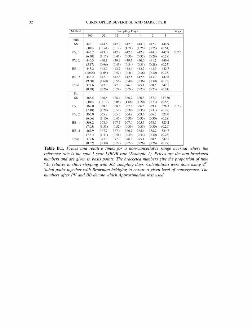
32 CHRISTOPHER BEVERIDGE AND MARK JOSHI
Method Sampling Days Vega365 52 12 6 4 2 1
mult.SS 443.1 444.6 442.2 442.3 444.0 442.7 444.9
(100) (13.41) (3.17) (1.71) (1.25) (0.75) (0.54)PV, 1 443.2 443.0 442.8 442.6 442.8 444.0 442.8 207.6
(6.70) (1.17) (0.46) (0.36) (0.32) (0.29) (0.28)PV, 2 440.3 440.1 439.9 439.7 440.0 441.2 440.6
(5.17) (0.96) (0.43) (0.34) (0.31) (0.28) (0.27)BB, 1 443.2 442.9 442.7 442.4 442.7 443.9 442.7
(10.05) (1.65) (0.57) (0.41) (0.36) (0.30) (0.28)BB, 2 443.2 442.9 442.8 442.5 442.8 443.9 442.8
(9.68) (1.60) (0.56) (0.40) (0.36) (0.30) (0.28)Chal. 377.6 377.3 377.0 376.3 375.1 368.5 342.1
(0.28) (0.26) (0.24) (0.24) (0.23) (0.23) (0.24)Pit.SS 368.5 366.8 368.4 366.2 366.3 357.9 327.36
(100) (13.19) (3.08) (1.68) (1.20) (0.73) (0.53)PV, 1 369.0 368.8 368.5 367.8 366.5 359.4 326.3 207.9
(7.48) (1.28) (0.50) (0.39) (0.35) (0.31) (0.28)PV, 2 366.0 365.8 365.5 364.8 363.6 356.5 324.0
(6.06) (1.10) (0.47) (0.36) (0.33) (0.30) (0.28)BB, 1 368.2 368.0 367.7 367.0 365.7 358.5 325.2
(7.95) (1.35) (0.52) (0.39) (0.35) (0.30) (0.29)BB, 2 367.9 367.7 367.4 366.7 365.4 358.2 324.7
(7.61) (1.31) (0.51) (0.39) (0.34) (0.30) (0.28)Chal. 377.6 377.3 377.0 376.3 375.1 368.5 342.1
(0.32) (0.30) (0.27) (0.27) (0.26) (0.26) (0.27)
Table B.1. Prices and relative times for a non-cancellable range accrual where thereference rate is the spot 1 year LIBOR rate (Example 1). Prices are the non-bracketednumbers and are given in basis points. The bracketed numbers give the proportion of time(%) relative to short-stepping with 365 sampling days. Calculations were done using 219
Sobol paths together with Brownian bridging to ensure a given level of convergence. Thenumbers after PV and BB denote which Approximation was used.
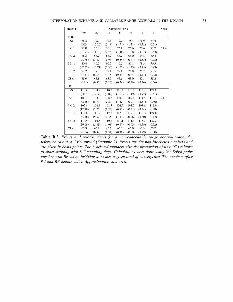
INTERPOLATION SCHEMES AND CALLABLE RANGE ACCRUALS IN THE DDLMM 33
Method Sampling Days Vega365 52 12 6 4 2 1
mult.SS 78.8 79.1 79.3 79.5 78.4 78.6 74.4
(100) (13.20) (3.19) (1.71) (1.21) (0.72) (0.51)PV, 1 77.0 76.9 76.9 76.8 76.6 75.6 71.7 21.4
(84.57) (11.18) (2.76) (1.48) (1.08) (0.64) (0.43)PV, 2 66.3 66.2 66.2 66.2 66.0 64.8 60.4
(22.76) (3.42) (0.96) (0.59) (0.47) (0.35) (0.28)BB, 1 80.4 80.3 80.3 80.3 80.1 79.3 76.3
(97.02) (13.74) (3.33) (1.77) (1.25) (0.75) (0.49)BB, 2 77.2 77.1 77.1 77.0 76.8 75.7 71.5
(37.27) (5.54) (1.45) (0.84) (0.64) (0.44) (0.33)Chal. 65.9 65.8 65.7 65.5 65.0 63.3 55.2
(0.31) (0.30) (0.27) (0.26) (0.26) (0.26) (0.26)Pit.SS 110.6 109.9 110.0 111.4 110.1 113.2 121.9
(100) (12.39) (3.07) (1.67) (1.19) (0.72) (0.51)PV, 1 108.7 108.6 108.7 109.0 109.4 111.5 119.4 21.9
(62.56) (8.71) (2.23) (1.22) (0.91) (0.57) (0.40)PV, 2 102.4 102.4 102.5 102.7 103.2 105.6 115.0
(17.70) (2.75) (0.82) (0.53) (0.44) (0.34) (0.29)BB, 1 112.0 111.9 112.0 112.3 112.7 115.0 124.0
(65.56) (9.52) (2.35) (1.31) (0.96) (0.60) (0.42)BB, 2 110.9 110.8 110.9 111.1 111.5 113.7 122.2
(26.09) (3.88) (1.09) (0.67) (0.53) (0.39) (0.32)Chal. 65.9 65.8 65.7 65.5 65.0 63.3 55.2
(0.35) (0.34) (0.31) (0.30) (0.30) (0.29) (0.30)
Table B.2. Prices and relative times for a non-cancellable range accrual where thereference rate is a CMS spread (Example 2). Prices are the non-bracketed numbers andare given in basis points. The bracketed numbers give the proportion of time (%) relativeto short-stepping with 365 sampling days. Calculations were done using 219 Sobol pathstogether with Brownian bridging to ensure a given level of convergence. The numbers afterPV and BB denote which Approximation was used.

34 CHRISTOPHER BEVERIDGE AND MARK JOSHI
Method Sampling Days Vega365 52 12 6 4 2 1
mult.SS 332.2 330.3 330.3 331.3 330.4 331.4 327.04
(100) (13.39) (3.15) (1.71) (1.20) (0.72) (0.50)PV, 1 328.9 328.5 328.5 328.4 328.4 327.9 324.5 27.6
(92.97) (13.42) (3.29) (1.77) (1.25) (0.75) (0.45)PV, 2 332.5 332.1 332.1 332.1 332.1 331.5 328.6
(30.86) (4.60) (1.22) (0.72) (0.55) (0.39) (0.30)BB, 1 331.0 330.6 330.6 330.6 330.6 330.4 328.0
(96.92) (13.28) (3.30) (1.73) (1.23) (0.73) (0.47)BB, 2 327.7 327.3 327.3 327.2 327.2 326.5 322.9
(96.92) (5.43) (1.42) (0.82) (0.62) (0.42) (0.32)Chal. 336.6 336.2 336.2 336.2 336.0 335.8 335.8
(0.30) (0.29) (0.26) (0.26) (0.26) (0.25) (0.25)Pit.SS 351.2 348.7 348.4 351.5 349.3 351.2 354.7
(100) (12.87) (3.12) (1.68) (1.21) (0.73) (0.49)PV, 1 349.5 349.2 349.2 349.3 349.5 350.5 353.1 28.3
(74.48) (10.63) (2.77) (1.47) (1.05) (0.65) (0.44)PV, 2 358.6 358.2 358.3 358.4 358.7 360.3 365.9
(28.50) (4.22) (1.16) (0.70) (0.55) (0.40) (0.32)BB, 1 351.1 350.7 350.8 350.9 351.1 352.2 356.5
(65.41) (9.61) (2.43) (1.33) (0.98) (0.62) (0.43)BB, 2 351.0 350.6 350.7 350.8 351.0 352.2 356.3
(26.46) (3.93) (1.11) (0.68) (0.54) (0.40) (0.32)Chal. 336.6 336.2 336.2 336.2 336.0 335.8 335.8
(0.35) (0.35) (0.31) (0.31) (0.30) (0.30) (0.29)
Table B.3. Prices and relative times for a non-cancellable range accrual where thereference rate is a CMS spread and there is a stochastic multiplier (Example 3). Pricesare the non-bracketed numbers and are given in basis points. The bracketed numbers givethe proportion of time (%) relative to short-stepping with 365 sampling days. Calculationswere done using 219 Sobol paths together with Brownian bridging to ensure a given levelof convergence. The numbers after PV and BB denote which Approximation was used.
Method Example1 2 3
mult.SS 5.71 (0.45) 1.72 (0.13) 3.33 (0.81)
PV, 1 6.88 (-0.84) 3.21 (3.16) 4.34 (4.34)PV, 2 7.60 (1.89) 14.01 (14.01) 5.08 (0.68)BB, 1 5.75 (-0.76) 1.17 (-0.55) 2.49 (1.85)BB, 2 5.79 (-0.80) 3.12 (3.12) 5.72 (5.72)Chal. 74.64 (74.64) 15.52 (15.52) 9.03 (-3.62)Pit.SS 11.62 (10.64) 2.60 (-2.60) 2.39 (-0.01)
PV, 1 9.81 (9.10) 1.21 (-0.91) 2.68 (0.70)PV, 2 12.18 (11.98) 5.00 (5.00) 10.82 (-9.10)BB, 1 10.35 (9.98) 4.38 (-4.38) 2.30 (-1.07)BB, 2 10.61 (10.27) 3.08 (-3.08) 3.26 (-1.07)Chal. 26.26 (0.04) 47.38 (47.38) 16.70 (15.34)
Table B.4. Sum of absolute errors (non-bracketed) and errors (bracketed) in the individualcoupon values. All numbers are in basis points. Calculations were done using 219 Sobolpaths together with Brownian bridging to ensure a given level of convergence. The numbersafter PV and BB denote which Approximation was used. Exact answers were obtainedusing short-stepping with 365 sampling days, while 2 sampling days were used to obtainthe results for the methods listed in the table.

INTERPOLATION SCHEMES AND CALLABLE RANGE ACCRUALS IN THE DDLMM 35
Method Delta Rate E. Vega Time1 4 7 10 13 16 19
PV, 12, FD -.326 -.033 .3539 .4539 .4662 .4474 .4146 .2865 555.92PV, 6, FD -.3236 -.0333 .3538 .4538 .4663 .4474 .4147 .2864 394.41PV, 4, FD -.3186 -.0334 .3538 .4537 .4664 .4474 .4148 .2865 340.19PV, 2, FD -.2951 -.0339 .3536 .4535 .4664 .4472 .4149 .2875 286.47PV, 12, Aprx -.3272 -.0324 .3539 .4537 .466 .4473 .4145 .2869 290.94PV, 6, Aprx -.3248 -.0327 .3538 .4537 .4661 .4472 .4146 .2868 238.55PV, 4, Aprx -.3198 -.0328 .3538 .4536 .4663 .4472 .4146 .2869 219.88PV, 2, Aprx -.2965 -.0333 .3537 .4534 .4662 .4471 .4147 .2879 205.31PV, 12, PC -.3272 -.033 .3539 .4539 .4663 .4475 .4147 .285 269.5PV, 6, PC -.3248 -.0332 .3538 .4539 .4664 .4475 .4148 .2849 228.98PV, 4, PC -.3199 -.0333 .3538 .4538 .4665 .4475 .4148 .2851 214.34PV, 2, PC -.2966 -.0338 .3536 .4536 .4665 .4473 .4149 .2861 203.08BB, 12, FD -.3225 -.032 .3551 .4542 .4695 .4464 .4158 .2867 952.47BB, 6, FD -.321 -.0325 .3551 .4541 .4695 .4464 .4157 .2867 610.89BB, 4, FD -.3164 -.0328 .3552 .4541 .4695 .4464 .4156 .2869 497.33BB, 2, FD -.2933 -.0335 .3554 .4541 .4694 .4466 .4154 .2879 384.72BB, 12, Aprx -.3229 -.032 .3551 .4542 .4695 .4464 .4158 .2871 372.97BB, 6, Aprx -.3213 -.0325 .3552 .4541 .4695 .4464 .4157 .2871 283.78BB, 4, Aprx -.3167 -.0328 .3553 .4541 .4695 .4464 .4156 .2873 258.95BB, 2, Aprx -.2937 -.0335 .3555 .4542 .4695 .4466 .4154 .2883 227.06BB, 12, PC -.3229 -.032 .3551 .4542 .4695 .4464 .4158 .2871 359.66BB, 6, PC -.3214 -.0325 .3551 .4541 .4695 .4464 .4157 .2871 275.8BB, 4, PC -.3167 -.0328 .3552 .4541 .4695 .4464 .4156 .2873 252.33BB, 2, PC -.2937 -.0335 .3555 .4541 .4694 .4466 .4154 .2883 225.05
Table B.5. Deltas, elementary vegas and times (in seconds) for a non-cancellable rangeaccrual where the reference rate is the spot 1 year LIBOR rate (Example 1) and ourmultiplicative interpolation scheme. Calculations were done using 219 Sobol paths.
Method Delta Rate E. Vega Time1 4 7 10 13 16 19
PV, 12, FD -.4076 -.0536 .3606 .4631 .4741 .4535 .42 .2329 435.94PV, 6, FD -.4047 -.0504 .3628 .4636 .4727 .4537 .4199 .2327 309.64PV, 4, FD -.4034 -.049 .3621 .464 .4736 .4528 .4194 .2317 265.48PV, 2, FD -.3893 -.0539 .3634 .4644 .4747 .4535 .42 .2271 225.02PV, 12, Aprx -.3892 -.0552 .3598 .4626 .4736 .4532 .4198 .233 275.78PV, 6, Aprx -.3861 -.0519 .362 .463 .4721 .4534 .4196 .2329 226.06PV, 4, Aprx -.3845 -.0506 .3612 .4634 .4731 .4525 .4191 .2319 209.73PV, 2, Aprx -.3687 -.0557 .3625 .4638 .4741 .4532 .4198 .2273 192.58PV, 12, PC -.3876 -.0553 .36 .4627 .4739 .4535 .4201 .2309 264.06PV, 6, PC -.3847 -.0517 .3625 .4634 .4727 .4537 .4197 .2308 221.44PV, 4, PC -.383 -.0504 .3614 .4637 .4732 .4528 .4194 .2297 207.55PV, 2, PC -.3673 -.0558 .3627 .464 .4747 .4534 .42 .2252 191.3BB, 12, FD -.4003 -.0454 .362 .4627 .4771 .4543 .4205 .2327 538.26BB, 6, FD -.3974 -.048 .363 .4629 .4759 .4535 .4207 .2321 375.92BB, 4, FD -.3953 -.0483 .3635 .4626 .4762 .4538 .4203 .2314 316.61BB, 2, FD -.3854 -.0487 .3635 .4637 .4771 .4548 .4195 .2267 261.23BB, 12, Aprx -.3961 -.0457 .3619 .4625 .477 .4542 .4205 .233 311.23BB, 6, Aprx -.3933 -.0484 .3629 .4628 .4758 .4534 .4207 .2324 249.12BB, 4, Aprx -.3911 -.0487 .3634 .4625 .4761 .4537 .4203 .2317 227.52BB, 2, Aprx -.3814 -.0489 .3634 .4636 .477 .4547 .4195 .227 207.14BB, 12, PC -.3956 -.0457 .3619 .4624 .4769 .454 .4206 .2328 306.92BB, 6, PC -.3927 -.0485 .3628 .4626 .4759 .4534 .4206 .2323 248.41BB, 4, PC -.3906 -.0489 .3634 .4623 .4761 .4538 .4204 .2315 226.73BB, 2, PC -.3809 -.049 .3634 .4632 .477 .4547 .4195 .2268 208.22
Table B.6. Deltas, elementary vegas and times (in seconds) for a non-cancellable rangeaccrual where the reference rate is the spot 1 year LIBOR rate (Example 1) and thePiterbarg interpolation scheme is used. Calculations were done using 219 Sobol paths.

36 CHRISTOPHER BEVERIDGE AND MARK JOSHI
Method Delta Rate E. Vega Time1 4 7 10 13 16 19
PV, 12, FD 1.6276 1.8919 .7067 .0712 -.5126 -.4451 -.1728 -.0753 11068.64PV, 6, FD 1.627 1.8922 .7067 .0712 -.5126 -.4451 -.1728 -.0754 5576.83PV, 4, FD 1.6258 1.8929 .7069 .0713 -.5127 -.4453 -.1729 -.0756 3765.31PV, 2, FD 1.6188 1.8961 .708 .0718 -.5133 -.4459 -.1732 -.0765 1940.41PV, 12, Aprx 1.6264 1.8975 .7113 .0765 -.5067 -.4397 -.17 -.0736 1005.64PV, 6, Aprx 1.6258 1.8979 .7113 .0764 -.5068 -.4398 -.1701 -.0738 556.98PV, 4, Aprx 1.6245 1.8986 .7115 .0765 -.5069 -.4399 -.1701 -.0739 404.98PV, 2, Aprx 1.6175 1.9021 .7128 .0771 -.5073 -.4406 -.1704 -.0747 256.22PV, 12, PC 1.6203 1.8875 .7143 .084 -.5024 -.4376 -.1694 -.079 459.31PV, 6, PC 1.6197 1.888 .7143 .0839 -.5024 -.4377 -.1694 -.0791 281.66PV, 4, PC 1.6182 1.8887 .7146 .0841 -.5025 -.4378 -.1695 -.0793 227.16PV, 2, PC 1.6103 1.8922 .7161 .0849 -.5028 -.4384 -.1698 -.0803 165.28BB, 12, FD 1.6278 1.894 .7083 .0684 -.5147 -.4449 -.1722 -.0753 26221.8BB, 6, FD 1.6273 1.8945 .7086 .0683 -.5148 -.4451 -.1723 -.0755 13834.81BB, 4, FD 1.6261 1.8951 .7089 .0682 -.5149 -.4453 -.1724 -.0757 8879BB, 2, FD 1.6197 1.898 .7104 .0683 -.5153 -.4461 -.1728 -.0769 4481.84BB, 12, Aprx 1.6271 1.8958 .709 .0688 -.5138 -.4439 -.1716 -.0738 1341BB, 6, Aprx 1.6266 1.8963 .7093 .0686 -.5139 -.4441 -.1717 -.0739 723.38BB, 4, Aprx 1.6255 1.897 .7096 .0686 -.5139 -.4442 -.1718 -.0741 526.69BB, 2, Aprx 1.6189 1.9001 .7112 .0687 -.5142 -.4449 -.1721 -.0751 323.78BB, 12, PC 1.6234 1.8927 .7102 .0713 -.5119 -.4426 -.1712 -.0754 829.2BB, 6, PC 1.6229 1.8932 .7104 .0712 -.512 -.4428 -.1713 -.0756 471.28BB, 4, PC 1.6216 1.8938 .7108 .0712 -.512 -.4429 -.1714 -.0758 352.22BB, 2, PC 1.6144 1.8967 .7126 .0716 -.5121 -.4435 -.1717 -.077 234.88
Table B.7. Deltas, elementary vegas and times (in seconds) for a non-cancellable rangeaccrual where the reference rate is a CMS spread (Example 2) and our multiplicativeinterpolation scheme. Calculations were done using 219 Sobol paths.
Method Delta Rate E. Vega Time1 4 7 10 13 16 19
PV, 12, FD 1.6427 1.9093 .7055 .0626 -.5143 -.4497 -.1755 -.0684 6388.14PV, 6, FD 1.6421 1.9099 .7056 .0625 -.5144 -.4498 -.1756 -.0685 3207.34PV, 4, FD 1.6411 1.9109 .7058 .0624 -.5145 -.4501 -.1757 -.0685 2168.92PV, 2, FD 1.6361 1.9162 .7067 .0617 -.5155 -.4513 -.1763 -.0689 1134.77PV, 12, Aprx 1.6358 1.9142 .7097 .0692 -.5076 -.4448 -.1727 -.068 757.59PV, 6, Aprx 1.6351 1.9148 .7098 .0691 -.5077 -.4449 -.1728 -.068 426.69PV, 4, Aprx 1.634 1.9159 .71 .069 -.5078 -.4451 -.1729 -.0681 317.89PV, 2, Aprx 1.6283 1.9213 .7109 .0685 -.5086 -.4465 -.1735 -.0684 209.56PV, 12, PC 1.633 1.9076 .7113 .0743 -.5046 -.4442 -.1727 -.0712 374.55PV, 6, PC 1.6322 1.9082 .7115 .0742 -.5047 -.4444 -.1728 -.0712 238.94PV, 4, PC 1.6311 1.9093 .7117 .0741 -.5048 -.4446 -.1729 -.0713 193.55PV, 2, PC 1.6251 1.915 .7127 .0737 -.5057 -.4461 -.1736 -.0716 146.06BB, 12, FD 1.6417 1.9112 .7097 .0593 -.5157 -.4499 -.175 -.0678 12216.14BB, 6, FD 1.6411 1.9119 .7099 .0593 -.5158 -.4501 -.1751 -.0679 5968.95BB, 4, FD 1.6402 1.9129 .7102 .0591 -.5159 -.4503 -.1752 -.068 4096.88BB, 2, FD 1.6355 1.9183 .7114 .0581 -.5169 -.4516 -.1758 -.0685 2104.17BB, 12, Aprx 1.6404 1.9121 .7098 .0601 -.5147 -.449 -.1744 -.0677 888.22BB, 6, Aprx 1.6397 1.9127 .7099 .0601 -.5148 -.4491 -.1744 -.0678 501.2BB, 4, Aprx 1.6388 1.9138 .7102 .0599 -.515 -.4493 -.1745 -.0679 369.33BB, 2, Aprx 1.6337 1.9192 .7115 .059 -.5158 -.4505 -.1751 -.0684 239.66BB, 12, PC 1.6388 1.9104 .71 .0615 -.5137 -.4484 -.1742 -.0685 634.02BB, 6, PC 1.6382 1.9111 .7102 .0615 -.5138 -.4485 -.1742 -.0685 377.23BB, 4, PC 1.6372 1.9121 .7105 .0614 -.5139 -.4487 -.1743 -.0687 285.67BB, 2, PC 1.6321 1.9173 .7117 .0605 -.5147 -.4498 -.1749 -.0692 200.38
Table B.8. Deltas, elementary vegas and times (in seconds) for a non-cancellable range ac-crual where the reference rate is a CMS spread (Example 2) and the Piterbarg interpolationscheme is used. Calculations were done using 219 Sobol paths.

INTERPOLATION SCHEMES AND CALLABLE RANGE ACCRUALS IN THE DDLMM 37
Method Delta Rate E. Vega Time1 4 7 10 13 16 19
PV, 12, FD 1.5379 1.1877 .2076 -.4118 -1.1341 -.6189 -.2352 .0183 14229.84PV, 6, FD 1.5375 1.1881 .2076 -.4117 -1.1344 -.619 -.2352 .0183 7183.92PV, 4, FD 1.5367 1.1886 .2078 -.4117 -1.1347 -.6193 -.2353 .0184 4805.5PV, 2, FD 1.5318 1.1918 .2089 -.4116 -1.1364 -.6205 -.2358 .0189 2512.34PV, 12, Aprx 1.5388 1.2036 .22 -.406 -1.1281 -.6151 -.234 .021 1212.42PV, 6, Aprx 1.5384 1.204 .2201 -.406 -1.1283 -.6153 -.234 .021 660.31PV, 4, Aprx 1.5376 1.2047 .2203 -.4059 -1.1286 -.6155 -.2341 .0212 479.48PV, 2, Aprx 1.5327 1.2082 .2214 -.4059 -1.1303 -.6168 -.2346 .0219 292.41PV, 12, PC 1.5307 1.1829 .2157 -.4004 -1.1168 -.6067 -.2309 .0142 647.41PV, 6, PC 1.5302 1.1833 .2158 -.4004 -1.117 -.6069 -.231 .0142 364.05PV, 4, PC 1.5292 1.1839 .216 -.4003 -1.1172 -.6071 -.231 .0143 276.67PV, 2, PC 1.5234 1.1873 .2174 -.4001 -1.1183 -.6083 -.2315 .0147 190.39BB, 12, FD 1.5384 1.1912 .2114 -.4166 -1.1383 -.6179 -.234 .0178 26205.61BB, 6, FD 1.538 1.1917 .2118 -.4167 -1.1385 -.6181 -.2341 .0178 13250BB, 4, FD 1.5373 1.1922 .2121 -.4168 -1.1387 -.6184 -.2342 .0178 8854.48BB, 2, FD 1.5328 1.1952 .2138 -.4169 -1.1399 -.6197 -.2348 .0179 4499.39BB, 12, Aprx 1.538 1.1926 .2114 -.4166 -1.1372 -.6162 -.233 .02 1337.23BB, 6, Aprx 1.5377 1.193 .2117 -.4168 -1.1373 -.6164 -.2331 .0201 728.64BB, 4, Aprx 1.5369 1.1936 .2121 -.4169 -1.1375 -.6167 -.2332 .0201 524.22BB, 2, Aprx 1.5324 1.1967 .2138 -.417 -1.1386 -.6179 -.2337 .0205 321.06BB, 12, PC 1.5345 1.1876 .2105 -.4159 -1.1343 -.6136 -.2321 .0162 817.38BB, 6, PC 1.5341 1.188 .2109 -.416 -1.1345 -.6138 -.2322 .0162 467.24BB, 4, PC 1.5333 1.1885 .2112 -.4161 -1.1345 -.614 -.2323 .0162 353.06BB, 2, PC 1.5282 1.1912 .213 -.4163 -1.1352 -.6149 -.2327 .0161 238.16
Table B.9. Deltas, elementary vegas and times (in seconds) for a non-cancellable rangeaccrual with stochastic multiplier and the reference rate is a CMS spread (Example 3), andour multiplicative interpolation scheme. Calculations were done using 219 Sobol paths.
Method Delta Rate E. Vega Time1 4 7 10 13 16 19
PV, 12, FD 1.5281 1.2014 .2203 -.3966 -1.1108 -.6208 -.2379 .0032 7320.42PV, 6, FD 1.5273 1.202 .2206 -.3965 -1.1107 -.6209 -.238 .0031 3714.92PV, 4, FD 1.5261 1.2029 .2211 -.3963 -1.1106 -.6212 -.2381 .0029 2521.83PV, 2, FD 1.5201 1.2079 .2234 -.3952 -1.1103 -.6228 -.2389 .0017 1316PV, 12, Aprx 1.5343 1.2146 .232 -.3901 -1.1062 -.6172 -.2365 .0035 929.59PV, 6, Aprx 1.5336 1.2152 .2323 -.39 -1.1062 -.6174 -.2366 .0033 526.48PV, 4, Aprx 1.5324 1.2161 .2328 -.3898 -1.1061 -.6177 -.2367 .0031 384.31PV, 2, Aprx 1.5269 1.2212 .2352 -.3886 -1.1058 -.6194 -.2375 .0019 245.28PV, 12, PC 1.529 1.1985 .2282 -.3842 -1.0957 -.6116 -.2345 .0001 526.44PV, 6, PC 1.5283 1.1991 .2286 -.384 -1.0956 -.6118 -.2346 -.0001 313.12PV, 4, PC 1.527 1.2 .2291 -.3838 -1.0955 -.6122 -.2348 -.0003 249.36PV, 2, PC 1.5211 1.2053 .2317 -.3823 -1.095 -.614 -.2356 -.0015 172.86BB, 12, FD 1.5277 1.2037 .2276 -.4022 -1.1107 -.6212 -.2376 .0036 12119.14BB, 6, FD 1.5269 1.2043 .2279 -.4019 -1.1107 -.6213 -.2377 .0034 6111.06BB, 4, FD 1.5258 1.2053 .2285 -.4016 -1.1107 -.6216 -.2378 .0031 4090.44BB, 2, FD 1.5201 1.2104 .2316 -.4008 -1.1102 -.6232 -.2386 .0016 2114.05BB, 12, Aprx 1.5276 1.2047 .2276 -.402 -1.1098 -.6198 -.2366 .0035 894.5BB, 6, Aprx 1.5269 1.2053 .2279 -.4017 -1.1098 -.6199 -.2366 .0033 501.03BB, 4, Aprx 1.5257 1.2063 .2285 -.4013 -1.1098 -.6202 -.2367 .003 378.59BB, 2, Aprx 1.5199 1.2114 .2316 -.4006 -1.1093 -.6216 -.2374 .0015 241.58BB, 12, PC 1.5258 1.2016 .2265 -.4006 -1.1075 -.6183 -.236 .0018 622.81BB, 6, PC 1.5251 1.2022 .2268 -.4003 -1.1075 -.6184 -.2361 .0015 370.03BB, 4, PC 1.5239 1.2031 .2274 -.4 -1.1074 -.6186 -.2362 .0012 282.34BB, 2, PC 1.5179 1.208 .2304 -.399 -1.1067 -.6198 -.2368 -.0004 195.83
Table B.10. Deltas, elementary vegas and times (in seconds) for a non-cancellable rangeaccrual with stochastic multiplier and the reference rate is a CMS spread (Example 3), andthe Piterbarg interpolation scheme is used. Calculations were done using 219 Sobol paths.

38 CHRISTOPHER BEVERIDGE AND MARK JOSHI
Example
12
3PV,1
PV,2BB,1
BB,2
PV,1PV,2
BB,1
BB,2
PV,1PV,2
BB,1
BB,2
mult.LS
794.3792.6
789.2789.5
879.6875.4
882.2880.2
709.6705.2
712.8707.3
SE1.6
1.61.8
1.8.7
.7.8
.8.9
.91
1SER
2.32.3
2.12.1
3.33.3
2.92.9
22.1
1.92
Time
73.472.5
73.173.5
7347.5
81.854
118.187.8
121.191.2
Paths524288
524288524288
524288524288
524288524288
524288524288
524288524288
524288Sobol
791.5789.9
792.2791.9
882.6878
883.5881.3
710.5705.6
713.1707.9
Time
9.39.1
8.98.9
4.62.9
5.13.3
7.25.3
7.65.5
Paths65536
6553665536
6553632768
3276832768
3276832768
3276832768
32768PI
13.313.3
11.512.8
3.13.4
3.33.1
8.99.1
8.78.3
SE2.1
2.32.3
2.31.3
1.31.2
1.21.8
1.31.9
1.8Tim
e22.7
22.427.6
26.64
24.8
2.738.5
27.546
32.3Paths
512512
512512
128128
128128
512512
512512
DG
26.727.9
26.927.3
7.27.6
9.99.8
15.916.6
17.217.5
SE1.5
1.61.6
1.6.7
.7.9
.91.4
1.41.7
1.8Vega
161.1162.6
158157.7
35.735.9
36.136
4.65.2
5.55.2
Pit.LS
762.9760.9
759.9759.8
907.2906.1
908.9908.4
723.1724.3
724.3722
SE1.7
1.71.8
1.8.7
.7.7
.7.9
.9.9
.9SER
2.22.2
2.12.1
3.13.2
3.13.1
22.1
22
Time
67.567.6
66.365.1
5942
62.346.1
95.775.4
90.974.9
Paths524288
524288524288
524288524288
524288524288
524288524288
524288524288
524288Sobol
761.3759.1
759.4760.1
906.5905.5
910.2909.3
722.4724
729.8727.2
Time
8.38.1
8.18
3.72.6
3.82.9
5.94.6
5.64.6
Paths65536
6553665536
6553632768
3276832768
3276832768
3276832768
32768PI
17.420.3
19.618.1
4.86
4.23.8
9.510.1
10.210.8
SE2
22
21.8
1.81.7
1.61.6
1.62.2
2.4Tim
e42.4
40.947.8
47.73.3
1.83.3
2.131.4
23.130.8
23.2Paths
10241024
10241024
128128
128128
512512
512512
DG
26.625.5
31.130.9
5.65.4
9.79.9
13.714
16.215
SE1.7
1.72
1.9.5
.5.8
.81.4
1.51.8
1.5Vega
151.6151
149.7148.5
35.435.4
36.236.1
4.16.1
4.24.3
TableB.11.
Callableprices
foreach
caseconsidered.Allprices
andstandard
errorsare
inbasis
points,andtim
esare
measured
inseconds.Allcalculations
weredone
usingMersenne
Twisterrandom
numbers,exceptfor
therow
labeledSobol,which
containsthe
least-squareslower
boundusing
Sobolquasi-randomnum
bers.Thenum
bersafter
PVand
BBdenote
whichApproxim
ationwas
used.LS
isused
todenote
theleast-squares
lowerbound,PIthe
improvem
entinthe
lowerbound
dueto
policyiteration,D
Gthe
distancebetween
theleast-squares
lowerbound
andthe
upperbound,SE
thestandard
errorand
SERthe
factorreduction
instandard
errorobtained
usingthe
deltahedge
controlvariatefrom
[5].Ineach
case,1500outer
andinner
pathswere
usedto
calculatethe
dualitygaps
and2
19paths
wereused
tocalculate
vegas.Ineach
case,2sam
plingdays
wereused
whensim
ulatingrange
accrualcoupons.

INTERPOLATION SCHEMES AND CALLABLE RANGE ACCRUALS IN THE DDLMM 39
Exam
ple
12
3PV
,1PV
,2BB,1
BB,2
PV,1
PV,2
BB,1
BB,2
PV,1
PV,2
BB,1
BB,2
mult.
E.Ve
ga.183
2.181
9.180
1.179
3-.0
233
-.026
7-.0
228
-.024
0.023
4.018
7.023
7.021
3Time
131.5
125.9
139.7
130.9
152.3
90.5
195.1
131.9
214.6
143.1
232.9
168.8
Paths
5242
8852
4288
5242
8852
4288
5242
8852
4288
5242
8852
4288
5242
8852
4288
5242
8852
4288
Pit.
E.Ve
ga.143
2.142
1.140
4.140
5-.0
174
-.019
7-.0
162
-.016
8.014
4.012
6.015
4.014
5Time
119.3
119.2
126.8
121.4
118.1
75.6
135.8
109.2
174.1
121.7
169
138.4
Paths
5242
8852
4288
5242
8852
4288
5242
8852
4288
5242
8852
4288
5242
8852
4288
5242
8852
4288
TableB.12
.Ca
llableGreek
results
foreach
case
considered.T
imes
aremeasuredin
seconds.Ca
lculations
were
done
usingSobol
random
numbers.T
henumbers
afterPV
andBB
denote
whichAp
proximationwa
sused.Ineach
case,4
samplingdays
were
used.

40 CHRISTOPHER BEVERIDGE AND MARK JOSHI
Centre for Actuarial Studies, Dept of Economics, University of Melbourne, Victoria 3010, AustraliaE-mail address: [email protected] address: [email protected]