Consistent interpolation of equidistantly sampled data
26
NUMERICAL LINEAR ALGEBRA WITH APPLICATIONS Numer. Linear Algebra Appl. 2009; 16:319–344 Published online 28 November 2008 in Wiley InterScience (www.interscience.wiley.com). DOI: 10.1002/nla.628 Consistent interpolation of equidistantly sampled data Eike Rietsch ∗, † Formerly Chevron Energy Technology Company, 15000 Louisiana St., Houston, TX 77002, U.S.A. SUMMARY Let u 1 , u 2 ,..., u N with u n ∈ R denote the values of a function recorded or computed at N real and equidis- tant abscissa values t n = nt + t 0 for n = 1,..., N . A consistent interpolation operator L, as defined in this paper, interpolates these function values for N new abscissas t n = (n + 1 2 )t + t 0 , the first N − 1 of which are halfway between those originally given while the last one is outside of the original abscissa range. Application of L to these interpolated function values produces the last N − 1 samples u 2 , u 3 ,..., u N of the original data plus one extrapolated function value u N +1 . Hence, L 2 is essentially a shift operator, but with a prediction component. The difference between various interpolation methods (e.g. polynomials, Fourier series) is now reduced to the way in which u N +1 is determined. This concept not only permits a uniform view at interpolation by quite different classes of functions but also allows the creation of more general interpolation, differentiation, and integration formulas, which can be tailored to particular problems. Copyright 2008 John Wiley & Sons, Ltd. Received 7 April 2008; Revised 24 September 2008; Accepted 26 October 2008 KEY WORDS: consistent interpolation; equidistant; prediction 1. INTRODUCTION A large amount of experimental and observational data are available in digital form, sampled equidistantly in one or more dimensions. Usually, great care is taken to assure that the data are not aliased, that they are recorded in such a way that the shortest period in the data is greater than twice the sample interval. Frequently, for display or further processing, the data need to be interpolated to a finer interval. A variety of tools are available for interpolating such equidistantly sampled data. A summary can be found, for example, in [1]. These methods are largely based on fitting a function to the data and evaluating this function at the desired abscissa values—though, for efficiency reasons, this function is not explicitly determined. A more recent history of interpolation techniques is in [2]. ∗ Correspondence to: Eike Rietsch, 14346 Carolcrest St., Houston, TX 77077, U.S.A. † E-mail: [email protected] Copyright 2008 John Wiley & Sons, Ltd.
-
Upload
independent -
Category
Documents
-
view
0 -
download
0
Transcript of Consistent interpolation of equidistantly sampled data
NUMERICAL LINEAR ALGEBRA WITH APPLICATIONSNumer. Linear Algebra Appl. 2009; 16:319–344Published online 28 November 2008 in Wiley InterScience (www.interscience.wiley.com). DOI: 10.1002/nla.628
Consistent interpolation of equidistantly sampled data
Eike Rietsch∗,†
Formerly Chevron Energy Technology Company, 15000 Louisiana St., Houston, TX 77002, U.S.A.
SUMMARY
Let u1,u2, . . . ,uN with un ∈R denote the values of a function recorded or computed at N real and equidis-tant abscissa values tn =n�t+t0 for n=1, . . . ,N . A consistent interpolation operator L, as defined in thispaper, interpolates these function values for N new abscissas tn =(n+ 1
2 )�t+t0, the first N−1 of whichare halfway between those originally given while the last one is outside of the original abscissa range.Application of L to these interpolated function values produces the last N−1 samples u2,u3, . . . ,uN ofthe original data plus one extrapolated function value uN+1. Hence, L2 is essentially a shift operator, butwith a prediction component. The difference between various interpolation methods (e.g. polynomials,Fourier series) is now reduced to the way in which uN+1 is determined. This concept not only permitsa uniform view at interpolation by quite different classes of functions but also allows the creation ofmore general interpolation, differentiation, and integration formulas, which can be tailored to particularproblems. Copyright q 2008 John Wiley & Sons, Ltd.
Received 7 April 2008; Revised 24 September 2008; Accepted 26 October 2008
KEY WORDS: consistent interpolation; equidistant; prediction
1. INTRODUCTION
A large amount of experimental and observational data are available in digital form, sampledequidistantly in one or more dimensions. Usually, great care is taken to assure that the data arenot aliased, that they are recorded in such a way that the shortest period in the data is greater thantwice the sample interval.
Frequently, for display or further processing, the data need to be interpolated to a finer interval.A variety of tools are available for interpolating such equidistantly sampled data. A summary canbe found, for example, in [1]. These methods are largely based on fitting a function to the dataand evaluating this function at the desired abscissa values—though, for efficiency reasons, thisfunction is not explicitly determined. A more recent history of interpolation techniques is in [2].
∗Correspondence to: Eike Rietsch, 14346 Carolcrest St., Houston, TX 77077, U.S.A.†E-mail: [email protected]
Copyright q 2008 John Wiley & Sons, Ltd.

320 E. RIETSCH
This paper reintroduces the concept of consistent interpolation apparently first conceived byFerrar [3, 4] to describe the shift-invariance ofWhittaker’s cardinal function of interpolation. Specialcases of this concept lead to well-known classical interpolation formulas (and their generalizations)and to a new class of interpolation formulas that are based on prediction error filters developedin digital signal analysis and that lead to interpolations, which turn out to be both accurate andstable.
The theory developed here is restricted to the interpolation of real-valued functions of a realvariable. This simplifies the derivation and was sufficient for the intended use of the method.However, for time series, where much of the theory has been developed for complex-valuedfunctions, an extension of the interpolation to so-called analytic signals appears straightforwardand potentially quite useful.
The most important result described in this paper is the fact that this concept provides ageneral, uniform view of different interpolation formulas. The distinguishing feature becomes—somewhat surprising for interpolation formulas—how they extrapolate outside the range of theknown data values.
2. CONSISTENT INTERPOLATION
Let u(t) denote a real-valued function of the real variable t , known at N equidistant abscissa valuestn = t0+n�t with n=1, . . . ,N . The N-tuple un =u(tn) represents the components of the vector uin RN . We assume that the Nyquist frequency, f� =1/(2�t), is greater than the highest frequencyin u(t) (basically, this means that in a Fourier representation of u(t) the highest frequency has aperiod greater than 2�t).
Assume that we want to compute u(t) for abscissa values tn+1/2= t0+(n+ 12 )�t , half-way
between the tn , and let L denote an interpolation operator such that
L{un}={un+1/2}i.e. L applied to the un generates the new function values un+1/2 at the abscissa values tn+1/2=t0+(n+ 1
2 )�t .Obviously, only the first N−1 samples un+1/2 are true interpolates. The abscissa tN+1/2 of the
last sample, uN+1/2, is outside the original range of abscissa values [t1, tN ]. Nevertheless, for thesake of simplicity, we generally refer to the {un+1/2} as interpolates.
From the point of view of the {un+1/2}, the last N−1 original samples un are interpolates, andthe interpolation operator is called consistent if it produces these N−1 original samples whenapplied to the N interpolated samples {un+1/2}.
L2{un}=L(L{un})=L{un+1/2}={un+1} (1)
Thus, the square of a consistent interpolation operator is essentially a shift operator with anextrapolation (or prediction) component that generates the last sample uN+1=u(t1+N�t). Consis-tency simply means that had we been given the interpolated values {un+1/2}, we could havecomputed the {un}. No information is lost when going from the {un+1/2} to the {un} and vice versa.{un+1/2} and {un} are completely equivalent representations of the underlying function u(t).
Consistent interpolation is more general than exact interpolation (which is designed to interpolatecertain classes of functions exactly [2]). Exact interpolation is by necessity consistent. The converse
Copyright q 2008 John Wiley & Sons, Ltd. Numer. Linear Algebra Appl. 2009; 16:319–344DOI: 10.1002/nla

CONSISTENT INTERPOLATION 321
is not necessarily true. Lagrange interpolation is exact and thus consistent; spline interpolation isgenerally neither exact nor consistent.
Since we want L{un+vn}=L{un}+L{vn} for any two N-tuples {un} and {vn}, L must be alinear operator. Since it operates on a vector, it is represented by a matrix.‡ From Equation (1) itfollows that L2 must have the form of a square matrix
L2=S=
⎛⎜⎜⎜⎜⎜⎜⎜⎜⎝
0 1 0 · · · 0
0 0 1 · · · 0
......
.... . .
...
0 0 0 · · · 1
1+a1 a2 a3 · · · aN
⎞⎟⎟⎟⎟⎟⎟⎟⎟⎠
(2)
S has the structure of the companion matrix [5, p. 12ff]; upon operating on the samples {un}, itproduces N−1 original samples (u2, . . . ,uN ) and one predicted (or extrapolated) function value(unless otherwise indicated, sums extend from 1 to N ).
uN+1=u1+∑anun (3)
For later analysis it is convenient to write
S=P+eNaT (4)
where
P=
⎛⎜⎜⎜⎜⎜⎜⎜⎜⎝
0 1 0 · · · 0
0 0 1 · · · 0
......
.... . .
...
0 0 0 · · · 1
1 0 0 · · · 0
⎞⎟⎟⎟⎟⎟⎟⎟⎟⎠
(5)
is a permutation matrix; en denotes a unit vector in RN , which has 1 as its nth component and zeroseverywhere else. The vector aT={a1,a2, . . . ,aN } is as yet undetermined and is to be chosen insuch a way that the unknown, extrapolated value uN+1 can be represented by a linear combinationof the known {un}. Thus,
L=S1/2=[P+eNaT]1/2 (6)
represents a consistent interpolation operator in the sense of the definition above, provided thematrix square root exists and is unique and real.
‡In this paper the terms operator and matrix are sometimes used interchangeably. The term ‘operator’ is mostlyused in a more general sense or when the effect on an operand is of concern; ‘matrix’ is generally used when theproperties of the operator itself are being discussed.
Copyright q 2008 John Wiley & Sons, Ltd. Numer. Linear Algebra Appl. 2009; 16:319–344DOI: 10.1002/nla

322 E. RIETSCH
The interpolation operator appears to have a kind of directivity. It is based on what one mightcall forward prediction or forward extrapolation. Clearly, there should be a completely equivalentoperator L̂ such that
L̂{un}={un−1/2} (7)
From L(L̂)=L{un−1/2}={un} for any {un}, it follows:
L̂L=I (8)
where I is the identity matrix. Hence, L̂=L−1. Matrices L and L−1 interpolate by extrapolatingin opposite directions.
3. PROPERTIES OF THE INTERPOLATION MATRIX L
For an interpolation operator to be generally useful, it should have certain properties. Here werequire the following:
1. Invariance with respect to the ‘interpolation direction’: L applied to the function values{uN ,uN−1, . . . ,u1} should produce the same N−1 interpolated values {uN−1/2,uN−3/2, . . . ,
u3/2} as L applied to {u1,u2, . . . ,uN }—just in reverse order.2. Exact interpolation of a constant: If all the components of u are equal to some constant, then
the interpolated samples should equal the same constant (the partition of unity condition).3. Stability with respect to ‘noise’: Small changes in the sample values should lead to small
changes in the interpolated values, i.e. the interpolation operator should not unduly amplifynumerical errors or data inaccuracies (noise).
3.1. Invariance
The first property is a plausible one that makes sense in many cases encountered in practice. Itis important to note, however, that there are situations where it may not be the most appropriatechoice—where a relaxation of this condition may lead to better results. Examples are sampledrepresentations of evolutionary or generally non-stationary processes. Such cases are disregardedhere.
This invariance requirement can be expressed as
LHu=HL−1u (9)
where
H=
⎛⎜⎜⎜⎜⎜⎝
0 · · · 0 1
0 · · · 1 0
... . .. ...
...
1 · · · 0 0
⎞⎟⎟⎟⎟⎟⎠ (10)
Copyright q 2008 John Wiley & Sons, Ltd. Numer. Linear Algebra Appl. 2009; 16:319–344DOI: 10.1002/nla

CONSISTENT INTERPOLATION 323
is the ‘backward identity’ permutation matrix [6, p. 28]. Letp0 = 1+a1, pn =an+1 for n=1, . . . ,N−1 (11)
pN = −1 (12)
Then the invariance condition leads to
p0=1, pn =−pN−n (13)
or
p0=−1, pn = pN−n (14)
i.e. the pn are either symmetric or antisymmetric.
ProofSince Equation (9) must hold for any u,
LH=HL−1
or, since HH=I,
L−1=HLH
Squaring both sides lead to
L−1L−1=S−1=HLHHLH=HSH (15)
Hence, the same symmetry condition must hold for S. With S defined in Equation (4), its inversecan be readily computed [6]. From PTP=I it follows
S= P(I+PTeNaT)=P(I+e1aT) (16)
S−1 = (I+e1aT)−1PT=(I− 1
1+eT1ae1aT
)PT=PT− 1
1+a1e1(Pa)T (17)
Substituting (16) and (17) for S and S−1 in (15) leads to
PT− 1
1+a1e1(Pa)T=HPH+HeNaTH=PT+e1(Ha)T
Hence
Ha=− 1
1+a1Pa
that reads explicitly as
aN+1−n = − 1
1+a1an+1 for n=1, . . . ,N−1
a1 = − a11+a1
(18)
Copyright q 2008 John Wiley & Sons, Ltd. Numer. Linear Algebra Appl. 2009; 16:319–344DOI: 10.1002/nla

324 E. RIETSCH
The last equation in (18) has two solutions
a1={0
−2(19)
Thus, the an must satisfy either
a1 = 0
aN+1−n = −an+1, n=1, . . . ,N−1(20)
or
a1 = −2
aN+1−n = an+1, n=1, . . . ,N−1(21)
Equations (20) and (21) are equivalent to (13) and (14), respectively. �
In terms of these pn , Equation (3) reads as
N∑n=0
pnun+1=0 (22)
3.2. Exact interpolation of a constant
Just like the first requirement this second requirement is generally meaningful, but not a condition‘sine qua non’. Many so-called ‘time series’ are zero-mean and in those cases this requirementmay be unnecessary. It leads to a restriction on the pn
N∑n=0
pn =0 (23)
ProofThe requirement can be written as
Lo=o
where o={1,1, . . . ,1} is a vector of ones. Thus, o must be an eigenvector of L, and �=1 must bethe associated eigenvalue. Since L and S have the same eigenvectors, o must also be an eigenvectorof S. From Equation (4) it follows:
So=Po+eN (aTo)=o
Consequently,
aTo≡∑an =0
which is equivalent to (23). �
For any antisymmetric pn satisfying Equation (13), this condition is always satisfied since inthis case
N∑n=1
pn =[N/2]∑n=0
(pn+ pN−n)=0
Copyright q 2008 John Wiley & Sons, Ltd. Numer. Linear Algebra Appl. 2009; 16:319–344DOI: 10.1002/nla
CONSISTENT INTERPOLATION 325
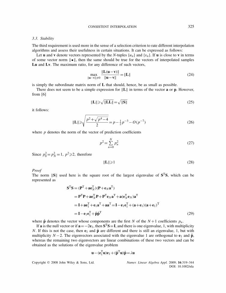
3.3. Stability
The third requirement is used more in the sense of a selection criterion to rate different interpolationalgorithms and assess their usefulness in certain situations. It can be expressed as follows:
Let u and v denote vectors represented by the N-tuples {un} and {vn}. If u is close to v in termsof some vector norm ‖•‖, then the same should be true for the vectors of interpolated samplesLu and Lv. The maximum ratio, for any difference of such vectors,
max‖u−v‖�=0
‖L(u−v)‖‖u−v‖ =‖L‖ (24)
is simply the subordinate matrix norm of L that should, hence, be as small as possible.There does not seem to be a simple expression for ‖L‖ in terms of the vector a or p. However,
from [6]‖L‖�√‖LL‖=√‖S‖ (25)
it follows:
‖L‖�√
p2+√p4−4
2= p− 1
2 p−3−O(p−7) (26)
where p denotes the norm of the vector of prediction coefficients
p2=N∑
n=0p2n (27)
Since p20 = p2N =1, p2�2, therefore
‖L‖�1 (28)
ProofThe norm ‖S‖ used here is the square root of the largest eigenvalue of STS, which can berepresented as
STS= (PT+aeTN )(P+eNaT)
= PTP+aeTNP+PTeNaT+a(eTN eN )aT
= I+aeT1 +e1aT+aaT=I−e1eT1 +(a+e1)(a+e1)T
= I−e1eT1 + p̂p̂T (29)
where p̂ denotes the vector whose components are the first N of the N+1 coefficients pn .If a is the null vector or if a=−2e1, then STS=I, and there is one eigenvalue, 1, with multiplicity
N . If this is not the case, then e1 and p̂ are different and there is still an eigenvalue, 1, but withmultiplicity N−2. The eigenvectors associated with the eigenvalue 1 are orthogonal to e1 and p̂,whereas the remaining two eigenvectors are linear combinations of these two vectors and can beobtained as the solutions of the eigenvalue problem
u−(eT1u)e1+(p̂Tu)p̂=�u
Copyright q 2008 John Wiley & Sons, Ltd. Numer. Linear Algebra Appl. 2009; 16:319–344DOI: 10.1002/nla

326 E. RIETSCH
The unknown coefficients, eT1u and p̂Tu, can be determined by multiplying this equation fromthe left by p̂T and eT1 , respectively. This leads to
(�−1)eT1u= −(eT1u)(eT1e1)+(p̂Tu)(eT1 p̂)
(�−1)p̂Tu= −(eT1u)(pTe1)+(p̂Tu)(p̂Tp̂)
a homogeneous system of equations whose eigenvalues �−1 are the two zeros of the quadratic
(�−1)2−( p̂2−1)(�−1)+1− p̂2=0
when the relations e1Te1=1,e1Tp= p0=1, and p̂2= p̂Tp̂ are used. Hence
�−1=
⎧⎪⎪⎪⎨⎪⎪⎪⎩
p̂2−1+√( p̂2+1)2−4
2
p̂2−1−√( p̂2+1)2−4
2
Obviously, the first of the two possible values for � is the larger one; with p2= p̂2+1, the desiredeigenvalue becomes
�= p2+√p4−4
2(30)
and this leads to the expression for the norm of S shown above. �
It is important to remember that ‖L‖ does not measure how close to the true values, theinterpolated values are, but rather how sensitive the vector u(1/2) is to changes in u.
4. COMPUTATION OF L
So far we have only performed formal operations. Now it needs to be shown that
1. L exists.2. L is real.3. L is unique.
4.1. Existence of L
Conditions for the existence of the square root of real matrices are well known [7]. To show theexistence of L at least for diagonalizable matrices, we note that any diagonalizable matrix S canbe represented as [6]
S=XRX−1 (31)
where X is a matrix whose N columns xn are the right eigenvectors of S and R is a diagonalmatrix whose diagonal elements are the eigenvalues, �n , of S. Then L=S1/2 can be written as
L=XR1/2X−1
Hence, a matrix L exists such that LL=S if S is diagonalizable.
Copyright q 2008 John Wiley & Sons, Ltd. Numer. Linear Algebra Appl. 2009; 16:319–344DOI: 10.1002/nla

CONSISTENT INTERPOLATION 327
An alternative way is to represent L in terms of a matrix polynomial in S
L=N−1∑m=0
bmSm (32)
The coefficients bm are solutions of the linear system of equations [6, 8]N−1∑m=0
bm�mn =√�n for n=1, . . . ,N (33)
The �n are the eigenvalues of S, and the generally complex Vandermonde matrix of this system isnon-singular, if they are all distinct; in this case (33) has a unique solution.
The rows of the matrix in (33) are simply the eigenvectors of xn of S and therefore, (33) canalso be written
XTb=r (34)
where the vector r represents vector of function of the eigenvalues—in this particular case, thesquare root.
4.2. Uniqueness and real-valuedness of L
Items 2 and 3 are closely connected. Since S is real the �n are either real or come in complexconjugate pairs. For L to be real as well, these complex conjugate pairs must remain complexconjugate after taking the square root of R. To this end we introduce a cut along the negative realaxis in the complex plane. A complex number, z, is thus defined by z=|z|exp(i�) for −�<���,and the square root of z,
√z=√|z|exp(i�/2), is unique.
There is, however, a problem with negative real eigenvalues. Since their square root is imaginary,they would lead to complex elements in L—in contradiction to requirement 2 above. It thus followsthat an interpolation matrix L=S1/2 that meets conditions 1, 2, and 3 does not exist, if S hasnegative real eigenvalues. To salvage the interpolation operator L for this particular case, we setnegative eigenvalues �n to zero before computing R1/2. Thus, we introduce a diagonal matrix Kwith diagonal elements
�n ={√
�n for �n �=−1
0 for �n =−1(35)
and
L=X−1KX (36)
In this way L remains real, but LL �=S. What this means in practice will be explained later inthe section on periodic functions for which S may indeed have a negative eigenvalue.
To illustrate the relationship between u and u(1/2), where u(1/2) denotes the vector with compo-nents {u1+1/2,u2+1/2, . . . ,uN+1/2}, we represent u in terms of the right eigenvectors of S, xn .
u=∑�nxn (37)
where
�n =�n(y∗nu) (38)
Copyright q 2008 John Wiley & Sons, Ltd. Numer. Linear Algebra Appl. 2009; 16:319–344DOI: 10.1002/nla

328 E. RIETSCH
with �n denoting the reciprocal of the inner product of the right and left eigenvectors xn and yn(Equation (A12)).
In analogy to Equation (A13), we can express L in terms of its right and left eigenvectors
L=∑�n�nxny∗n (39)
Hence,
u(1/2) =Lu=∑�n�nxn(y∗nu)=∑�n�nxn (40)
Interpolated values are represented by a linear combination of the right eigenvectors. Eigenvec-tors whose eigenvalues are negative are dropped from this sum because of (35).
Let �m be a negative eigenvalue of S. Then the associated eigenvectors xm and ym are real.Let u=cxm with real c �=0. From (40) and the definition of � (Equation (35)) it follows that theinterpolated values of a function whose samples are given by any multiple of xm are zero. Thusu(1/2) =0. The components of xm must alternate in sign. Equation (A3) shows that this is indeedthe case for any real �<0. In other words, in this case u are the values of a function that alternatesin sign at the sample points and has zeros halfway between the sample points. After interpolationwe are left with zeros and any information about the value of c is lost.
So, while a negative eigenvalue of S poses a problem that needs to be dealt with, in practice itis only important if (y∗u) �=0. But if this case occurs there is a problem with the underlying datathat needs to be addressed: the data have not been sampled finely enough or should have beenpre-filtered with a more severe anti-alias filter.
5. DIFFERENTIATION AND INTEGRATION
The interpolation operators discussed so far interpolate function values exactly half way betweenthe known nodes (sample points). It is quite obvious that this is but a special case of a moregeneral interpolation operator. Clearly, S1/M is an operator that interpolates function values forabscissas t0+(n+1/M)�t from those at abscissas t0+n�t (M-fold application of the operatorshifts all samples by one sample interval). Hence, we define the difference quotient
DM = M
�t(S1/M −I)
whose limit for M→∞ is an estimate of the derivative at the abscissas t0+n�t . Hence, wecompute a derivative operator
limM→∞DM = lim
M→∞M
�t
(exp
(1
MlnS
)−I)
(41)
= 1
�tlim
M→∞∞∑n=1
M1−n
n! (lnS)n = 1
�tlnS (42)
The matrix functions used above exist and are unique for all the cases considered in thispaper. Also, the power series expansion for the exponential function converges for every matrix[8, p. 336]. In the following, we shall call D= lnS the derivative operator.
Copyright q 2008 John Wiley & Sons, Ltd. Numer. Linear Algebra Appl. 2009; 16:319–344DOI: 10.1002/nla

CONSISTENT INTERPOLATION 329
For diagonalizable matrices S, the derivative operator is given by
D=XDX−1, D= logR (43)
The integration operatorQ is, in principle, the inverse of D. However, because of the requirementthat the interpolation operator should be exact for any constant (Section 3.2), one of the eigenvaluesof S is unity and its logarithm is 0. Thus D is singular, and Q must be expressed in terms of thegeneralized inverse of D.
After these general results, let us turn to special cases.
6. INTERPOLATION MATRIX L FOR PERIODIC FUNCTIONS
In the context of consistent interpolation this represents the simplest case. The N-tuple {un} isperiodic with period N if the {un} are part of an infinite sequence for which umN+n =un for anyinteger n and m. The predicted sample uN+1 equals the first sample u1. This means that all anare zero (see Equation (3)) and Equation (22) is satisfied for p0=1, pN =−1. S is simply thepermutation matrix P. The characteristic polynomial is
p(�)≡�N −1=0
The N eigenvalues of S are the N th roots of unity. In compliance with the above conventionregarding the complex plane, they can be written as
�n ={exp(�i(N+1−2n)/N ) for odd N
exp(�i(N−2n)/N ) for even N(44)
They are all different, and so S1/2 exists.However, for even N =2m the eigenvalue �m is equal to −1. The associated eigenvector is
xm =(1,−1, . . . ,−(−1)N )T
Its components, xn , (the subscript m has been dropped) are the samples of a cosine at the Nyquistfrequency f� =1/(2�t)
xn =−cos(2� f�n�t)=−cos(�n)
To illustrate the problem, let us use the function u(t)=ccos(2� f�t) with real c �=0 and f�denoting the Nyquist frequency 1/(2�t). If this function is sampled at times tn = t0+n�t , then
un =u(tn)=ccos(2� fntn)=(−1)nccos(�t0/�t)
What is sampled is essentially a random number from the interval [−c c] since un depends entirelyon t0, i.e. the instance when recording began. If t0 was an odd multiple of �t/2, nothing wouldbe recorded—no matter how large c is. This is the reason why properly digitized data have beenfiltered prior to sampling or why other means have been employed to remove periods that areequal to or shorter than twice the sampling interval. If this is the case, then (y∗
Nu)=0, and thefact that xNy∗
N , a matrix of rank 1, has been dropped from the representation (39) of L has nopractical consequences. It disregards components that should not be there in the first place.
Copyright q 2008 John Wiley & Sons, Ltd. Numer. Linear Algebra Appl. 2009; 16:319–344DOI: 10.1002/nla

330 E. RIETSCH
This problem is, of course, well known. Schoenberg [9], for example, introduced the conceptof ‘proximity interpolant’ for handling this problem with an even number of nodes. See also [10].
From (A7) it follows y= x̄; the left eigenvectors are the complex conjugate of the right eigen-vectors. Since P is a circulant, S is a circulant as well.
Furthermore, if L is orthogonal, LTL=I. Thus ‖L‖=1. Because of (28), this means that theinterpolation operator of periodic functions is as stable (robust with respect to noise) as possible.
ProofFrom STS=I, it follows LTLTLL=I. Let LTL = I+B. Then
LTLTLL=LT(I+B)L=I+B+LTBL=I
and B must satisfy
B+LTBL=0
This means B=0. �
7. INTERPOLATION MATRIX L FOR POLYNOMIALS
Interpolation by means of polynomials is a well-known method that can be easily implementedby means of the Lagrange interpolation formula [11]. Its serious problems, such as the Rungephenomenon [12], are also well known, and the main objective here is to show how it fits intothis consistent interpolation scheme and how its stability—as defined earlier and measured by thematrix norm ‖L‖—compares with that of other interpolation schemes discussed here. Furthermore,consistent interpolation allows a generalization that is less sensitive to data variations.
In order to determine the interpolation matrix L for this case, it is necessary to chose the {pn}such that Equation (22) is satisfied if the {un} are sampled polynomials of degree <N . This isequivalent to demanding that
N∑n=0
pn(tn− t0)k =�t
N∑n=0
pnnk =0 for k=0, . . . ,N−1
It is well known [13, p. 4] that this condition is satisfied if
pn =(−1)N−n+1
(N
n
)(45)
Obviously, the pn so defined also satisfy Equation (22) as well as Equations (13) or (14) for oddor even N , respectively.
The characteristic polynomial is
p(�) :=N∑
n=0(−1)n
(N
n
)�n =(1−�)N =0 (46)
and thus S has one eigenvalue, �1=1, with algebraic multiplicity N . There is only one eigenvector,x=o/‖o‖, associated with this eigenvalue. Hence, S is defective and cannot be diagonalized.
Copyright q 2008 John Wiley & Sons, Ltd. Numer. Linear Algebra Appl. 2009; 16:319–344DOI: 10.1002/nla
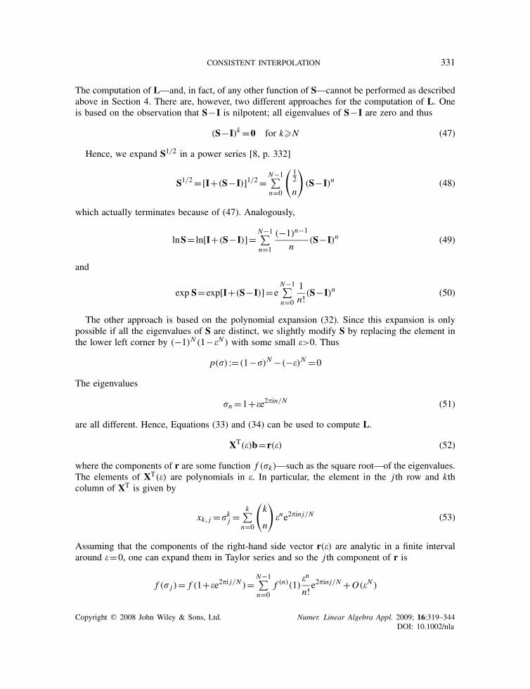
CONSISTENT INTERPOLATION 331
The computation of L—and, in fact, of any other function of S—cannot be performed as describedabove in Section 4. There are, however, two different approaches for the computation of L. Oneis based on the observation that S−I is nilpotent; all eigenvalues of S−I are zero and thus
(S−I)k =0 for k�N (47)
Hence, we expand S1/2 in a power series [8, p. 332]
S1/2=[I+(S−I)]1/2=N−1∑n=0
(12
n
)(S−I)n (48)
which actually terminates because of (47). Analogously,
lnS= ln[I+(S−I)]=N−1∑n=1
(−1)n−1
n(S−I)n (49)
and
exp S=exp[I+(S−I)]=eN−1∑n=0
1
n! (S−I)n (50)
The other approach is based on the polynomial expansion (32). Since this expansion is onlypossible if all the eigenvalues of S are distinct, we slightly modify S by replacing the element inthe lower left corner by (−1)N (1−N ) with some small >0. Thus
p(�) :=(1−�)N −(−)N =0
The eigenvalues
�n =1+e2�in/N (51)
are all different. Hence, Equations (33) and (34) can be used to compute L.
XT()b=r() (52)
where the components of r are some function f (�k)—such as the square root—of the eigenvalues.The elements of XT() are polynomials in . In particular, the element in the j th row and kthcolumn of XT is given by
xk, j =�kj =k∑
n=0
(k
n
)ne2�inj/N (53)
Assuming that the components of the right-hand side vector r() are analytic in a finite intervalaround =0, one can expand them in Taylor series and so the j th component of r is
f (� j )= f (1+e2�i j/N )=N−1∑n=0
f (n)(1)n
n!e2�inj/N +O(N )
Copyright q 2008 John Wiley & Sons, Ltd. Numer. Linear Algebra Appl. 2009; 16:319–344DOI: 10.1002/nla

332 E. RIETSCH
where the exponent in parentheses denotes the order of the derivative. Multiplication of XT
from the left with a row vector whose j th component is e−2�imj/N leads to a row vector whosecomponents are
N∑j=1
�kje−2�imj/N =
k∑n=0
(k
n
)n
N∑j=1
e2�i(n−m) j/N =N
(k
m
)m (54)
Likewise, multiplication of r by this row vector leads to a term
Nm
m! f(m)(1)+O(N+m)
which only contains the mth power of and terms of order N+m or greater.This results in the equation
Nm
m!N−1∑k=m
k!(k−m)!bk =N
m
m! f(m)(1)+O(N+m)
Dividing by the common factors and going to the limit →0 leads to
N−1∑k=m
k!(k−m)!bk = f (m)(1) (55)
Performing this operation for all m from 0 to N−1, one gets the following system of equationsfor the unknown coefficients bn:⎛
⎜⎜⎜⎜⎜⎜⎜⎜⎝
1 1 1 1 1 . . . 1
0 1 2 3 4 . . . N−1
0 0 2 6 12 . . . (N−1)(N−2)
......
......
......
...
0 0 0 0 0 . . . (N−1)!
⎞⎟⎟⎟⎟⎟⎟⎟⎟⎠
⎛⎜⎜⎜⎜⎜⎜⎜⎜⎝
b0
b1
b2
...
bN−1
⎞⎟⎟⎟⎟⎟⎟⎟⎟⎠
=
⎛⎜⎜⎜⎜⎜⎜⎜⎜⎜⎝
f (1)
f (1)(1)
f (2)(1)
...
f (N−1)(1)
⎞⎟⎟⎟⎟⎟⎟⎟⎟⎟⎠
Since all the diagonal elements are non-zero, this matrix is non-singular, and the system of equationshas a unique solution.
While not particularly important in this case (since there are other possibilities), this approachis useful in those cases where p(z) has both distinct and multiple roots—for example, one rootwith multiplicity M and N−M simple roots. Under those circumstances, a generalization of thefirst approach (creating a nilpotent matrix) is not obvious and, on the other hand, (34) cannot beused either.
The notorious instability of polynomial interpolation of equidistantly sampled functions [12] isreflected in the exponential increase of ‖L‖ with polynomial degree. From
p2=N∑
n=0
(N
n
)2
=(2N
N
)(56)
Copyright q 2008 John Wiley & Sons, Ltd. Numer. Linear Algebra Appl. 2009; 16:319–344DOI: 10.1002/nla

CONSISTENT INTERPOLATION 333
[13, p. 4] and (26) follows (with a kind of Sterling-formula expansion):
‖L‖2� 4N√(�N )
(1+O
(1
N
))(57)
Hence, small errors may grow exponentially with the degree of the polynomial used for interpo-lation.
8. INTERPOLATION MATRIX FOR STATIONARY TIME SERIES
The concept of weakly stationary time series has been developed to describe and analyze recordingsof observations as diverse as electromagnetic radiation from outer space, brain waves, speech, andseismic signals [14], to name just a few. The attribute ‘weakly stationary’ refers to the assumptionthat certain statistical properties of the time series—such as mean, variance, and in particular theautocovariance—do not change with time. This means that the expectation value E{un um} dependsonly on the difference |n−m| and not on the specific values of n and m and, with the ergodicityassumption, can be written as
E{un un+k}=ak = limN→∞
1
2N+1
N∑�=−N
u�u�+k (58)
where the ak represent the samples of the autocorrelation function [15, 16]. With this result wereturn to Equation (22), which represents a relationship to be satisfied by the coefficients of theprediction error filter for {un}. Rather than defining it for the specific set of un , we choose it insuch a way that it is good for all time series with the same autocorrelation function.
Obviously, this requires one to rephrase the condition in a somewhat softer form, requestingthat p to be chosen in such a way that the expectation value of the squared error is minimum.
E
{(N∑
n=0pnun
)2}=
N∑n=0
N∑m=0
pn pmE{unum}=N∑
n=0
N∑m=0
pnan−m pm =min (59)
So the objective is to find a vector p that minimizes (59) subject to the constraints
pn+ pN−n =0, p0=1, pN =−1 (60)
or
pn− pN−n =0, p0=−1, pN =−1,N∑
n=0pn =0 (61)
In view of the important role of p for the stability of the interpolation operator (see Equation (26)),the condition
p2=N∑
n=0p2n =small (62)
might be added.Rather than finding the general solution of (59) subject to (60) or (61), we restrict ourselves
to a partial solution subject to (62) and the last two equations in (60). With these constraints, the
Copyright q 2008 John Wiley & Sons, Ltd. Numer. Linear Algebra Appl. 2009; 16:319–344DOI: 10.1002/nla
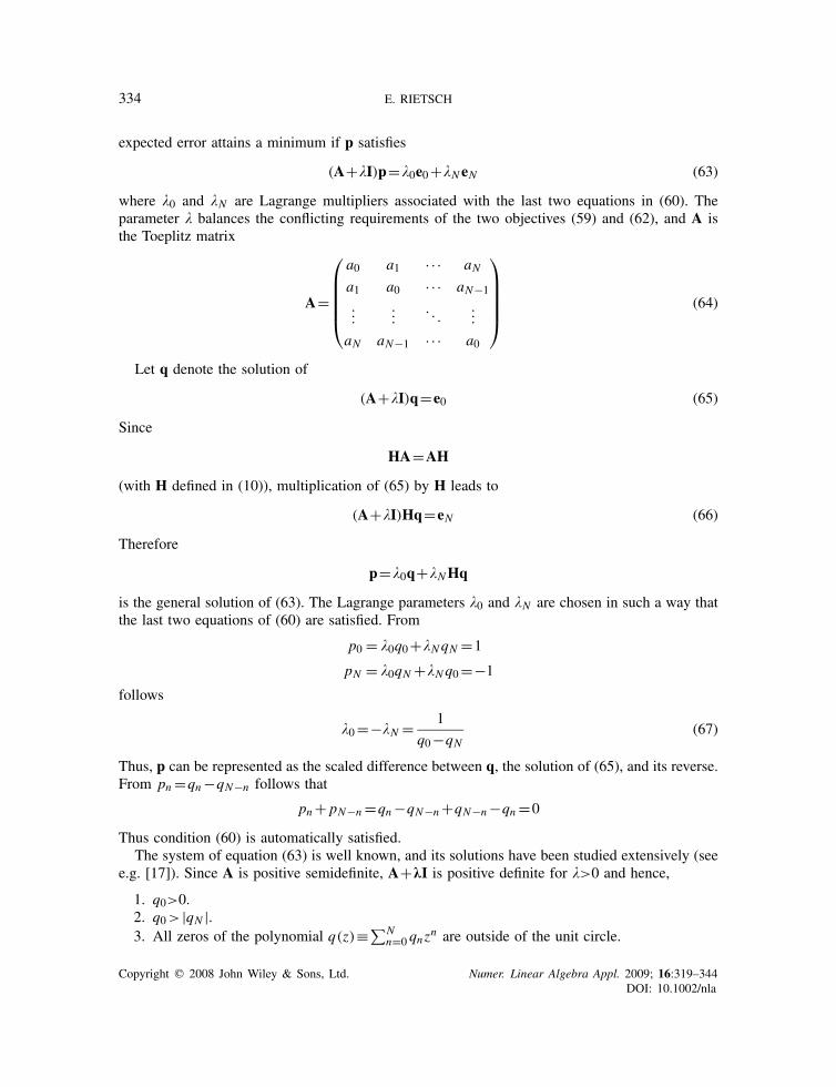
334 E. RIETSCH
expected error attains a minimum if p satisfies
(A+�I)p=�0e0+�N eN (63)
where �0 and �N are Lagrange multipliers associated with the last two equations in (60). Theparameter � balances the conflicting requirements of the two objectives (59) and (62), and A isthe Toeplitz matrix
A=
⎛⎜⎜⎜⎜⎝a0 a1 · · · aNa1 a0 · · · aN−1
......
. . ....
aN aN−1 · · · a0
⎞⎟⎟⎟⎟⎠ (64)
Let q denote the solution of
(A+�I)q=e0 (65)
Since
HA=AH
(with H defined in (10)), multiplication of (65) by H leads to
(A+�I)Hq=eN (66)
Therefore
p=�0q+�NHq
is the general solution of (63). The Lagrange parameters �0 and �N are chosen in such a way thatthe last two equations of (60) are satisfied. From
p0 = �0q0+�NqN =1
pN = �0qN +�Nq0=−1
follows
�0=−�N = 1
q0−qN(67)
Thus, p can be represented as the scaled difference between q, the solution of (65), and its reverse.From pn =qn−qN−n follows that
pn+ pN−n =qn−qN−n+qN−n−qn =0
Thus condition (60) is automatically satisfied.The system of equation (63) is well known, and its solutions have been studied extensively (see
e.g. [17]). Since A is positive semidefinite, A+kI is positive definite for �>0 and hence,
1. q0>0.2. q0> |qN |.3. All zeros of the polynomial q(z)≡∑N
n=0 qnzn are outside of the unit circle.
Copyright q 2008 John Wiley & Sons, Ltd. Numer. Linear Algebra Appl. 2009; 16:319–344DOI: 10.1002/nla

CONSISTENT INTERPOLATION 335
From the second item follows that q0+qN>0, and hence (67) exists. From the third statementfollows that all zeros of the polynomial p(z) :=∑N
n=0 pnzn are on the unit circle (Section A.2).
Consequently, the interpolation is performed by non-harmonic sine and cosine functions whoseperiods were chosen on the basis of the autocovariance function of the time series to be interpolated.In practice, this autocovariance function is approximated by the autocorrelation function of thetime series.
9. EXAMPLE
The following example is meant to illustrate the interpolation method for a short signal (160ms)consisting of two sine waves with frequencies of 60 and 85Hz, respectively. The signal had beencomputed with a sample interval of 4ms; hence, the maximum frequency was below the Nyquistfrequency of 125Hz.
The top panel of Figure 1 shows this superposition of the two sine waves. The known functionvalues are represented by solid black squares, the interpolated ones by open squares. The lower panelshows the interpolation errors. They are about an order of magnitude smaller than errors committedby cubic–spline interpolation and, not unexpectedly, tend to be higher toward the ends of the intervalover which the interpolation was performed. These end effects are caused by deficiencies in thecomputation of the vector p that required knowledge of the autocorrelation function. To illustratethis point, the dashed line (open squares) in Figure 2 shows the correct autocorrelation functionof the superposition of the two sines, normalized to 1 for zero lag; in practice, this function is notnormally known. The solid black squares show the autocorrelation function computed from the 41samples of the signal after tapering with a Papoulis window [18]. Obviously, the agreement betweenthe two deteriorates with increasing lag. It was the latter autocorrelation function that was used tocompute the Toeplitz matrix A and then solve Equation (63) for p with � set to 0.01. Once p isknown, S could be computed and from it the interpolation matrix L. Even though the autocorrelationfunction used was far from perfect, the interpolation result was quite good. However, a predictionfilter computed with a more sophisticated algorithm that directly computes the prediction filterwill, for this example, reduce the errors by an additional two orders of magnitude.
Incidentally, the value of � chosen for Equation (63) was simply the default; setting it to zerodid not noticeably change the result. It slightly raised the value of p2 (Equation (27)) from 5.2828to 5.3125, though, thus indicating a slight increase in the interpolation’s sensitivity to noise (keepin mind that the lowest possible value is 1).
Figure 3 shows the zeros of the characteristic polynomial. As proved in Appendix Sections A.2and A.3, these zeros are always on the unit circle but, except for periodic data, they are notuniformly distributed.
10. FINAL REMARKS
The paper reintroduced the concept of consistent interpolation of equidistantly sampled functionvalues and used its defining criteria to derive a general algorithm for its implementation. It assumedthat the function to be interpolated, while having infinite support, is only known on a finite set ofequidistant points (nodes) and that the function value at the first sample point outside this set canbe obtained from the known function values by linear prediction.
Copyright q 2008 John Wiley & Sons, Ltd. Numer. Linear Algebra Appl. 2009; 16:319–344DOI: 10.1002/nla

336 E. RIETSCH
0 20 40 60 80 100 120 140 160–2
–1.5
–1
–0.5
0
0.5
1
1.5
2
Time (ms)
Original and interpolated function values
0 20 40 60 80 100 120 140 160–0.05
–0.04
–0.03
–0.02
–0.01
0
0.01
0.02
0.03Interpolation error
Time (ms)
Figure 1. Top panel: Superposition of two sine functions. The black squares represent the initially knownfunction values and the open squares the interpolated values. Bottom panel: Interpolation error.
Copyright q 2008 John Wiley & Sons, Ltd. Numer. Linear Algebra Appl. 2009; 16:319–344DOI: 10.1002/nla

CONSISTENT INTERPOLATION 337
0 20 40 60 80 100 120 140 160–1
–0.8
–0.6
–0.4
–0.2
0
0.2
0.4
0.6
0.8
1Autocorrelation functions
Lag (ms)
Figure 2. The dashed line and open squares show the normalized autocorrelation function of the superpo-sition of the two sines; the black squares connected by solid lines represent the windowed autocorrelation
of the 41 samples to be interpolated.
–1 –0.5 0 0.5 1–1
–0.8
–0.6
–0.4
–0.2
0
0.2
0.4
0.6
0.8
1Roots of the characteristic polynomial
Figure 3. Roots of the characteristic polynomial. This figure illustrates their non-uniformdistribution on the unit circle.
Copyright q 2008 John Wiley & Sons, Ltd. Numer. Linear Algebra Appl. 2009; 16:319–344DOI: 10.1002/nla

338 E. RIETSCH
The paper also showed how special cases of this concept lead to interpolation by harmonicfunctions (Fourier series) and polynomials. If information about the general behavior of the functionis provided in the form of its autocorrelation function, this information can be used to implicitlydefine basis functions, which generally are non-harmonic sines and cosines (in special cases,not discussed here, the basis functions can be combinations of low-degree polynomials and non-harmonic sines and cosines).
An interesting aspect of the algorithm is that it allows one to assess the sensitivity of theinterpolated values to small changes of the original function values. This highlights, for example, theknown problems of equidistant polynomial interpolation as well as the stability of the interpolationof equidistantly sampled periodic function by harmonic sines and cosines.
For functions that can be regarded as weekly stationary, constraints on the variance of theparameter vector p allow one to make the interpolation more or less sensitive to data errors. Italso provides a way to select basis functions of inharmonic sines and cosines for interpolation.
As illustrated by the way the differentiation matrix was defined, the interpolation can beperformed for any rational fraction of the original sample interval.
APPENDIX A
A.1. Eigenvalues and Eigenvectors of S
Any eigenvalue � and the components, xn , of the associated right eigenvector x of
S=P+eNaT
must satisfy
xn+1 = �xn for n=1, . . . ,N−1 (A1)
x1+∑anxn = �xN (A2)
From (A1) it follows:
xn =c�n−1 (A3)
for some constant c.Substitution of (A3) for xn in (A2) and replacing the an by the pn defined in (11) leads to the
characteristic polynomial
p(�) :=N∑
n=0pn�
n =0 (A4)
S is simply the so-called companion matrix of p(�) [19]. Since p0 �=0 (see (13) and (14)), �=0is not a solution of (A4). Thus S is non-singular. But it is easy to show that �=1 is a zero ofp(�), if the pn satisfy condition (13). In this case �=−1 is also a zero of p(�), if N is even.The components, yn , of the left eigenvector y of ST with eigenvalue � satisfy
(1+a1)yN = �∗y1 (A5)
yn−1+an yN = �∗yn for n=2, . . . ,N (A6)
Copyright q 2008 John Wiley & Sons, Ltd. Numer. Linear Algebra Appl. 2009; 16:319–344DOI: 10.1002/nla

CONSISTENT INTERPOLATION 339
which leads to
y∗n =c
n−1∑m=0
pm�m−n =−cN∑
m=npm�m−n (A7)
where c is a normalization constant to make ‖y‖=1.
ProofLet
yn = zn(�∗)−n
Then (A6) reads as
zn−1+an yn(�∗)n−1= zn for n>1
Thus
zn = ynn∑
m=1am(�∗)m−1+c
and
yn = yN (�∗)−Nn∑
m=1am(�∗)m−1+c(�∗)−N
with some as yet arbitrary constant c. In particular, for n=N ,
yN = yN (�∗)−NN∑
m=1am(�∗)m−1+c(�∗)−N (A8)
= yN [1−(�∗)−N ]+c(�∗)−N (A9)
since, by virtue of (A4),
N∑m=1
am(�∗)m−1=(�∗)N −1
and hence yN =c. Thus, with (11),
yn =cn∑
m=1pm(�∗)m−n =
N∑m=n
pm(�∗)m−n (A10)
The constant c is now a factor that can be used to normalize the eigenvector. �
If all N zeros �1, . . . ,�N of p(�) are distinct, then S has N linearly independent eigenvectorsand can be diagonalized
S=XRX−1 (A11)
where X denotes a matrix whose columns are the right eigenvectors of S and R=diag(�1, . . . ,�N ).
Copyright q 2008 John Wiley & Sons, Ltd. Numer. Linear Algebra Appl. 2009; 16:319–344DOI: 10.1002/nla

340 E. RIETSCH
Since
X−1=CY∗
where C is a diagonal matrix whose diagonal elements
�n =1/(y∗nxn) (A12)
are the reciprocals of the inner product of the right and left eigenvectors associated with eacheigenvalue. It then follows that
S=XRCY∗ =∑�n�nxny∗n (A13)
A.2. Eigenvectors on the unit circle
In all cases considered here |�n|=1. The eigenvectors associated with distinct eigenvalues arethen sampled exponential functions with purely imaginary argument and form the generally non-orthogonal basis vectors of a vector space in much the same way as the harmonic exponentialfunctions form the basis vectors in the discrete Fourier domain.
For practical purposes—and to make the analogy more apparent—we shall also use the indexingscheme (in the following called ‘symmetry indexing’) described below.
Assume that the �n are sorted by increasing phase and start counting at index −[(N−1)/2].Since the eigenvalues come in complex conjugate pairs, �−� =�� and, in particular, �0=1. Also,for even N , �N =−1.
An important feature of this indexing scheme is that the higher the |�|, the more oscillatory arethe components of the eigenvectors associated with the �±�.
A.3. Zeros of the characteristic polynomial—antisymmetric case
Let
p(z)=q(z)−zNq(1/z) (A14)
denote an N th degree polynomial and q(z) an M th degree polynomial with real coefficients andN�M . All M zeros zm of q(z) are outside the unit circle; there is an >0 such that for all zeros zm
|zm |�1+ (A15)
Obviously, p(1)=0 and thus z=1 is always a zero of p(z), regardless of where the zeros ofq(z) are located. Furthermore, for even N , p(−1)=0 and thus z=−1 is also a zero of p(z).
Here we shall prove:
(A) All N zeros of p(z) are on the unit circle.(B) All N zeros of p(z) are distinct.
To prove proposition (A), let z=ei =1/z̄ and divide (A14) by zN/2. For p(z) to be zero onthe unit circle, it is necessary that
q(z)z̄N/2−q(z̄)zN/2=−2(q(z̄)zN/2)=0 (A16)
where the bar denotes complex conjugation. It follows from (A16) that on the unit circle p(z) iszero, whenever (q(z̄)zN/2) is zero. To prove proposition (A), it is thus necessary to show that
Copyright q 2008 John Wiley & Sons, Ltd. Numer. Linear Algebra Appl. 2009; 16:319–344DOI: 10.1002/nla

CONSISTENT INTERPOLATION 341
(q(z̄)zN/2)=|q(z)|sin(N/2+arg(q(z̄))) has N zeros. Since all zeros of q(z) are outside of theunit circle, |q(z)|>0 on the unit circle, and thus (A16) reduces to
sin(�())=0 (A17)
where
�()=N/2+arg(q(e−i)) (A18)
We assert that
(a) �() is a strictly monotonically increasing function of in the interval [0,2�].(b) �(0)=0, �(2�)=N�.
With zm =|zm |exp(i�m)
q(z̄)=q0M∏
m=1(1− z̄/zm)= q̄0
M∏m=1
|1− z̄/zm |exp[i arctan
(sin(+�m)
|zm |−cos(�+�m)
)]
Hence
�()=N/2+∑marctan
(sin(+�m)
|zm |−cos(+�m)
)(A19)
and
d
d��()=N/2+∑
m
( −1+|zm |cos(+�m)
1+|zm |2−2|zm |cos(+�m)
)
The terms in the above sum take their largest values, (|zm |−1)−1, for +�m =0,2� and theirsmallest value, −(|zM |+1)−1, for +�m =�. Hence, because of (A15),
d
d��() � N
2+ M
|zm |−1� N
2+ M
d
d��() � N
2− M
|zm |+1� N
2− M
2+�2(N−M)+N
(4+2)>0
(A20)
Thus, �() has a positive derivative in [0,2�] and is therefore strictly monotonic; this provesassertion (a).
From (A19) it follows that �(0)=0,�(2�)=N�, and this proves assertion (b).Since � is continuous and increases monotonically from 0 to N� for increasing from 0 to
2�, there are N values n in the interval [0,2�) such that �(n)=(n−1)� for n=1, . . . ,N . Forthese n , Equation (A17) is satisfied. These are all N zeros of p(z).
To prove proposition (B) we note that
�(n+1)−�(n)=�=(n+1−n)d
d��()/=x
�(n+1−n)(N/2+M/)
where n�x�n+1. Likewise,
�(n+1)−�(n)=�=(n+1−n)d
d��()/=x
�(n+1−n)2(N−m)+N
4+2
Copyright q 2008 John Wiley & Sons, Ltd. Numer. Linear Algebra Appl. 2009; 16:319–344DOI: 10.1002/nla

342 E. RIETSCH
Thus, the arguments of two consecutive zeros of p(z) satisfy the inequality
4+2
2(N−M)+N�n+1−n�
2�
N+2M>0 (A21)
For N �2M
2�
N
(1+ M
N (2+)
)�n+1−n�
2�
N
(1− 2M
N
)(A22)
the distribution of the zeros on the unit circle approaches the uniform distribution characteristicfor periodic functions.
A.3.1. Special case if q(z) has a root for z=1. Let q(z) denote an M th degree polynomial withreal coefficients that has one root at z=1 and whose other M−1 roots are outside the unit circle.Then
p(z) :=q(z)−zNq(1/z) (A23)
with N>M, is an N th degree polynomial that has distinct roots on the unit circle. Furthermore,for even N , z=−1 is also a root of p(z). Essentially, this means that this single root of q(z) onthe unit circle does not change the properties of p(z).
ProofLet q(z)=(1−z)q̂(z). Then
p(z)=(1−z)q̂(z)−zN(1− 1
z
)q̂
(1
z
)=(1−z)
[q̂(z)+zN−1q̂
(1
z
)](A24)
The term in brackets in the last part of (A24) has the same form as p(z) in Equation (A25). Hence,it has N−1 zeros on the unit circle, none of which is at z=1; however, for even N−1, one ofthese is at z=−1. This completes the proof. �
A.4. Zeros of the characteristic polynomial—symmetric case
Let
p(z)=q(z)+zNq(1/z) (A25)
denote an N th degree polynomial and q(z) an M th degree polynomial with real coefficients andN�M . All M zeros zm of q(z) are outside the unit circle; thus, there is an >0 such that for allzeros zm of q(z)
|zm |�1+ (A26)
Obviously, for odd N , p(−1)=q(−1)+(−1)Nq(−1)=0, and thus z=−1 is a zero of p(z).However, since p(1)=2q(1) �=0, there is never a zero at z=1.
In the following we shall prove the following:
(A) All N zeros of p(z) are on the unit circle.(B) All N zeros of p(z) are distinct.
Copyright q 2008 John Wiley & Sons, Ltd. Numer. Linear Algebra Appl. 2009; 16:319–344DOI: 10.1002/nla

CONSISTENT INTERPOLATION 343
To prove proposition (A), let z=ei =1/z̄ where the bar again denotes complex conjugationand divide (A25) by zN/2. For p(z) to be zero on the unit circle, it is necessary that
q(z)z̄N/2+q(z̄)zN/2=−2�(q(z̄)zN/2)=0 (A27)
It follows from (A27) that on the unit circle p(z) is zero whenever �(q(z̄)zN/2) is zero. To proveproposition (A), it is thus necessary to show that �(q(z̄)zN/2)=|q(z)|cos(N/2+arg(q(z̄))) hasN zeros. Since all zeros of q(z) are outside of the unit circle, |q(z)|>0 on the unit circle, and thus(A27) reduces to
cos(�())=0 (A28)
where
�()=N/2+arg(q(e−i)) (A29)
As shown in Appendix Section A.2 above this is indeed the case.Since � is continuous and increases monotonically from 0 to N� for increasing from 0 to
2�, there are N values n in the interval [0,2�) such that �(n)=(2n−1)�/2 for n=1, . . . ,N .For these n Equation (A17) is satisfied. These are all N zeros of p(z).
To prove proposition (B) we note that
�(n+1)−�(n)=�=(n+1−n)d
d�()/=x
�(n+1−n)(N/2+M/)
where n�x�n+1. Likewise,
�(n+1)−�(n)=�=(n+1−n)d
d�()/=x
�(n+1−n)2(N−m)+N
4+2
Thus, the arguments of two consecutive zeros of p(z) satisfy the inequality
4+2
2(N−M)+N�n+1−n�
2�
N+2M>0 (A30)
For N �2M
2�
N
(1+ M
N (2+)
)�n+1−n�
2�
N
(1− 2M
N
)(A31)
the distribution of the zeros on the unit circle approaches the uniform distribution characteristicfor periodic functions.
Furthermore, the zeros of p(z) in the symmetric case are bracketed by the zeros of the anti-symmetric case.
A.4.1. Special case if q(z) has a root for z=1. Let q(z) denote an M th degree polynomial with realcoefficients that has one root at z=1 and whose other M−1 roots are outside the unit circle. Then
p(z) :=q(z)+zNq(1/z) for N>M (A32)
is an N th degree polynomial that has a double root at z=1. The other N−2 roots are distinct andon the unit circle. Furthermore, for odd N , z=−1 is also a root of p(z).
Copyright q 2008 John Wiley & Sons, Ltd. Numer. Linear Algebra Appl. 2009; 16:319–344DOI: 10.1002/nla

344 E. RIETSCH
ProofLet q(z)=(1−z)q̂(z). Then
p(z)=(1−z)q̂(z)+zN(1− 1
z
)q̂
(1
z
)=(1−z)
[q̂(z)−zN−1q̂
(1
z
)](A33)
The term in brackets in the last part of (A33) has the same form as p(z) in Equation (A14). Hence,it has one zero at z=1, and all the other zeros are on the unit circle; for even N−1, one of theseis at z=−1. This completes the proof. �
ACKNOWLEDGEMENTS
I am indebted to Texaco for the permission to publish this paper.
REFERENCES
1. Crochiere RE, Rabiner LR. Multirate Digital Signal Processing. Prentice-Hall: Englewood Cliffs, NJ, 1983.2. Meijering E. A chronology of interpolation from ancient astronomy to modern signal and image processing.
Proceedings of the IEEE 2002; 90(3):319–342.3. Ferrar WL. On the cardinal function of interpolation theory. Proceedings of the Royal Society of Edinburgh 1926;
46:323–333.4. Ferrar WL. On the consistency of cardinal function interpolation. Proceedings of the Royal Society of Edinburgh
1927; 47:230–242.5. Wilkinson JH. The Algebraic Eigenvalue Problem. Oxford University Press: London, 1965.6. Horn RA, Johnson CR. Matrix Analysis. Cambridge University Press: Cambridge, 1992.7. Higham N. Computing real square roots of a real matrix. Linear Algebra and its Applications 1987; 88/89:
405–430.8. Mirsky L. An Introduction to Linear Algebra. Dover: New York, NY, 1990.9. Schoenberg IJ. Notes on spline functions. I. The limits of the interpolating periodic spline function as their
degree tends to infinity. Indagationes Mathematicae 1972; 34:412–423.10. Brass H. Optimal estimation rules for functions of high smoothness. IMA Journal of Numerical Analysis 1990;
10:129–136.11. Hildebrand FB. Introduction to Numerical Analysis. Academic Press: New York, NY, 1987.12. Lanczos C. Applied Analysis. Prentice-Hall: Englewood Cliffs, NY, 1956.13. Gradshteyn IS, Ryzhik IM. Table of Integrals, Series, and Products. Academic Press: New York, 1980.14. Robinson EA. Physical Applications of Stationary Time Series. Charles Griffin & Company Ltd.: London, 1980.15. Blackman RB, Tuckey JW. The Measurement of Power Spectra from the Point of View of Communications
Engineering. Dover: New York, NY, 1959.16. Thomas JB. An Introduction to Statistical Communication Theory. Wiley: New York, NY, 1969.17. Golub GH, Loan CFV. Matrix Computations. John Hopkins Series in the Mathematical Sciences. The John
Hopkins University Press: Baltimore, London, 1989.18. Papoulis A. Signal Analysis. McGraw-Hill: New York, NY, 1977.19. Ciarlet PG. Introduction to Numerical Linear Algebra and Optimization. Cambridge University Press: Cambridge,
1988.
Copyright q 2008 John Wiley & Sons, Ltd. Numer. Linear Algebra Appl. 2009; 16:319–344DOI: 10.1002/nla