http

://do

c.re

ro.c

h

Power Laws from Randomly-Sampled

Continuous-Time Random Walks

Giancarlo Mosetti a,b,1 Giancarlo Jug a,c Enrico Scalas a,d

aISI Foundation, Viale S.Severo 65, 10133 Torino (Italy)bDepartment de Physique, Chemin du Musee 3, Universite de Fribourg, CH-1700

Fribourg (Switzerland)cDipartimento di Fisica e Matematica, Universita dell’Insubria, Via Valleggio 11,

22100 Como (Italy)dDipartimento di Scienze e Tecnologie Avanzate, Universita del Piemonte

Orientale, Via Bellini 25 g, 15100 Alessandria (Italy)

Abstract

It has been shown by Reed that random-sampling a Wiener process x(t) at times T

chosen out of an exponential distribution gives rise to power laws in the distributionP (x(T )) ∼ x(T )−β . We show, both theoretically and numerically, that this power-law behaviour also follows by random-sampling Levy flights (as continuous-timerandom walks), having Fourier distribution w(k) = e−|k|α, with the exponent β = α.

Key words: Continuous Time Random Walks; Population Dynamics; Power Laws.PACS: 02.50.Cw, 87.23.2n, 89.65.Cd

1 Introduction

Many stochastic processes in various branches of the physical, economicaland social sciences present empirical power-law behaviour. A much discussedmechanism in recent years for this behaviour has been that of self-organisedcriticality (1). Reed has argued (2), on the other hand, that for a random-walk-like stochastic process, the power-law behaviour follows most naturally whenthe process’ measurement times T are also taken from a random distribution

1 To whom correspondence should be addressed:mosetti@isi.it - tel. +39 0116603090 - fax +39 011 6600049

Published in "Physica A: Statistical Mechanics and its Applications 375(1): 233-238, 2006" which should be cited to refer to this work.

http

://do

c.re

ro.c

h

(e.g. exponential: fT (t) = Λe−Λt). This would account in a phenomenologicalway for many empirically-observed power laws in many stochastic phenomena.

In Economics prime examples of such laws are the distribution of incomes(Pareto’s law (3)) and city sizes (Zipf’s law (4)), as well as - arguably - ofthe standardised price returns on generic stocks or on stock indices (5; 6). Inother realms of investigation, empirical size distributions for which power-lawbehaviour has been claimed include those of granular media’s particle sizes(7); of avalanche sizes (1); of meteor impact’s on the moon (8); of numberof species per genus (9); of frequency of words in long sequences of text (4);of areas of burnt patches in forest fires (10); and so on. In Physics, power-laws are observed in static and dynamic correlation functions at the criticalpoint of a second-order phase transition; in the non-equilibrium transportphenomena pertaining to the so-called 1/f-noise (11), or Barkhausen noisein the context of magnetism, (12); and so on. Within and outside the fieldsof application of the laws of physics the presence of power-law probabilitydistributions P (x) = C x−β appears to be ubiquitous and in the overwhelmingmajority of cases a prediction of the value of the exponent β from the lawswhich determine the local behaviour of the system is lacking.

For this reason, Reed’s proposal appears as an interesting explanation on aphenomenological standpoint for the ubiquity of the power-law distributionwhenever a stochastic process is observed: for observations also take place atobservation times which are themselves stochastically chosen.

In fact, to fix our ideas, let us consider a geometric random-walk process x(t)modelled by the stochastic differential equation

dx = μxdt + σxdw (1)

where dw is the increment in time dt of a Wiener process, σ a diffusion coeffi-cient and μ a drift bias. The distribution function of such process is lognormal,as is well known, however many stochastic processes modelled by this type ofdynamics do show up power-law behaviours empirically. When Ito’s calculus(13) is applied, the probability density for y = ln x is known to be, at a generictime t

P (y, t) =1√

2πσ2texp{−[y − y(0) − (μ − σ2/2)t]2/2σ2t} (2)

and has moment-generating function

My(s) = 〈eys〉Py= exp{y1s +

1

2y2

2s2} (3)

2

http

://do

c.re

ro.c

h

where 〈·〉Pyis the average with respect to the density in Eq. (2) and the first

two moments are given by y1 = y(0) + (μ − σ2/2)t and y2 = σ√

t as in astandard geometric random-walk process (where y(0) = ln x(0) refers to theinitial conditions).

Now we assume that the observation times t = T themselves are taken from arandom-variable probability density fT (t), which we may assume to be of theexponential type (this being the only memoryless case):

fT (t) = Λe−Λt, for Λ > s (4)

where Λ is the sampling rate. The moment-generating function for the variabley = y(T ) is now given by the conditional average over the observation-timesdistribution as well:

My(s)=⟨〈eys〉Py

⟩fT

= ey(0)s Λ

Λ − (μ − σ2/2)s − σ2s2/2(5)

At this point, we can seek the two real poles s1, s2 (with s1 > 0 and s2 < 0)of the above expression to obtain the form

My(s) = ey(0)s s1s2

(s − s1)(s − s2)(6)

which, thought of as a new moment-generating function gives the density

P (y) =

⎧⎪⎨⎪⎩| s1s2

s1−s2|e−s1(y−y(0)) if y > y(0)

| s1s2

s1−s2|e−s2(y−y(0)) if y < y(0)

(7)

These exponential contributions provide, for the variable x itself, the soughtpower-law,

P (x) =

⎧⎪⎨⎪⎩| s1s2

s1−s2| 1x(0)

(x

x(0)

)−s1−1if x > x(0)

| s1s2

s1−s2| 1x(0)

(x

x(0)

)−s2−1if 0 ≤ x < x(0)

(8)

2 Models based on continuous-time random walks (CTRW)

Our point of view is that, for example in the case of high-frequency financialreturns, assuming a geometric random walk process for the random variable

3

http

://do

c.re

ro.c

h

x(t) is somewhat unrealistic when looking at the available empirical data. Infact, trading in financial markets is an asynchronous process since durationsbetween consecutive trading events are random variables (14). In such a case,x(t) has the meaning of the price of an asset and y(t) can be considered asthe log-price or the log-return with respect to the initial price. We thereforepropose an improvement of the ’microscopic’ modelling by a continuous-timerandom-walk (CTRW), as the raw stochastic process with jumps, ξ, describedby a generalised Fourier representation of the density function characterisedby a form

w(k) = e−|k|α (9)

with α a real parameter in [0, 2]. Eq. (9) is the characteristic function of a so-called Levy α-stable random variable. The underlying stochastic dynamics isthen characterised by randomly-spaced jumps of random amplitudes, ξ, whichmore faithfully mimic the actual pricing dynamics of the financial marketsand other relevant situations. As another example for our model, we can con-sider the growth of firms and enterprises (or of atomic islands in appropriatephysics contexts) where x(t) is the firm’s size. The CTRW jumps arising atrandom times are asynchronous idiosyncratic shocks, or growth rates, and oursubordination to the exponential process corresponds to the fact that firmsare monitored at random times. In this way, our model differs from Reed’ssituation in that the waiting times between two adjacent size values are alsorandom variables (a situation closer to reality).

In this context, we recall that Gibrat has claimed the discovery (15) of asimple law that can explain the origin of inequalities within economic growthprocesses (16). A simple equation that takes into account the ideas of Gibratis as follows (17):

x(t + 1) = η(t)x(t) (10)

where x(t) represents the firm’s size and η(t) is a random variable alwaysextracted from the same probability distribution at any discrete period t. Eq.(10) is a growth model with multiplicative noise. It is the basis on whichthe so-called generalized Lotka-Volterra models are built (18). There are nodirect or indirect interactions between the firms, and the logarithm of the size,y(t) = ln x(t), is the sum of independent and identically distributed randomvariables, the growth rates ξ = ln η:

y(t + 1) = y(0) +t∑

m=1

ξ(m) (11)

4

http

://do

c.re

ro.c

h

If the growth rate is independent from the size, the Central Limit Theoremand its generalisations apply in the large t limit and one gets either normal orLevy distributed log-sizes and, therefore, log-normal or log-Levy distributedsizes. In a situation in which the growth shocks, ξ, can arrive at random timesinstead of at fixed periods, Eq. (11) must be replaced by its continuous-timecounterpart, given by the non-homogeneous form:

y(t) = y(0) +n(t)∑m=1

ξ(m). (12)

where n(t) is the number of shocks up to time t. These ideas have been recentlyapplied by economists to models of firm growth (19). It is important to remarkthat the probability distribution for y follows either a normal or anomalousdiffusive behaviour (17).

We now show that implementing the random sampling-time idea of Reed, apower-law behaviour is obtained for the distribution function of the variabley = y(T ).

3 Random sampling of CTRW

3.1 Analytical approach

If we assume Poisson waiting times and Levy distributed jumps 2 , the overalldisplacement density is given by:

P (y, t) =∞∑

N=0

(λt)Ne−λt

N !w∗N

(y) (13)

The Fourier Transform of (13) is

P (k, t) =∞∑

N=0

(λt)Ne−λt

N !wN(k) = eλt(e−|k|α−1) (14)

where w(k) = e−|k|α is the characteristic function of the Levy symmetric stabledistribution with exponent α and λ is the rate for the CTRW jumps. In thefirm-growth interpretation, λ is the rate of arrival of the idiosyncratic shocks.

2 In the following we will assume that the scale factor that usually appears in thedefinition of the characteristic function of a Levy distributions is simply c = 1

5

http

://do

c.re

ro.c

h

As in Reed’s case, the observation times t = T are taken as a random variablesdistributed with rate Λ, fT (t) = Λe−Λt, and averaging over observation timesEq. (14) gives:

P (k) =

∞∫0

dt Λe−Λteλt(w(k)−1) =Λ

Λ + λ(1 − w(k))(15)

The next step is to find the inverse Fourier Transform of (15) in order to getP (y). After some algebraic manipulation, one finds:

P (k) =Λλ

(Λ + λ)2

∞∑n=0

(λ

Λ + λ

)n

[w(k)]n+1 +Λ

Λ + λ(16)

that implies

P (y) =Λλ

(Λ + λ)2

∞∑n=0

(λ

Λ + λ

)n

w∗n+1

(y) +Λ

Λ + λδ(y) (17)

Observing that [w(k)]n = e−n|k|α it is not difficult to argue that the δ functioncan be formally written as w∗0

(x). This allows us to write the expression (17)in a more compact form,

P (y) =Λ

Λ + λ

∞∑n=0

(λ

Λ + λ

)n

w∗n

(y) (18)

Finally, from the stable property of w(k), it is possible to express the convo-lution of Levy densities in the following way:

w∗n

(y) = n− 1

α w(n− 1

α y)

(19)

3.2 Simulation vs analytical results

A closer look to eq. (15) allows us to verify the analytical results discussed inthe previous section. For example, if we want the behaviour of P (y) for largevalues of y we have to consider eq. (15) for values of k near to zero. One cancheck that

P (k) ∼ 1 − λ

Λ|k|α ∼ e−λ|k|α/Λ. (20)

But this is exactly the Fourier Transform of a Levy distributions with exponentα and implies that the pdf of our process has got a power-law tail with the

6

http

://do

c.re

ro.c

h

1e+01 1e+02 1e+03 1e+04 1e+05

1e−

071e

−05

1e−

03

y

P>(y

)α = 1.1

CCDFAy−α

−1e+07 0e+00 5e+06

1e−

071e

−03

y

y

1e+01 1e+02 1e+03 1e+04 1e+05

1e−

071e

−05

1e−

03

CCDFBy−α

α = 1.7

−80000 −40000 0 20000

1e−

071e

−03

y

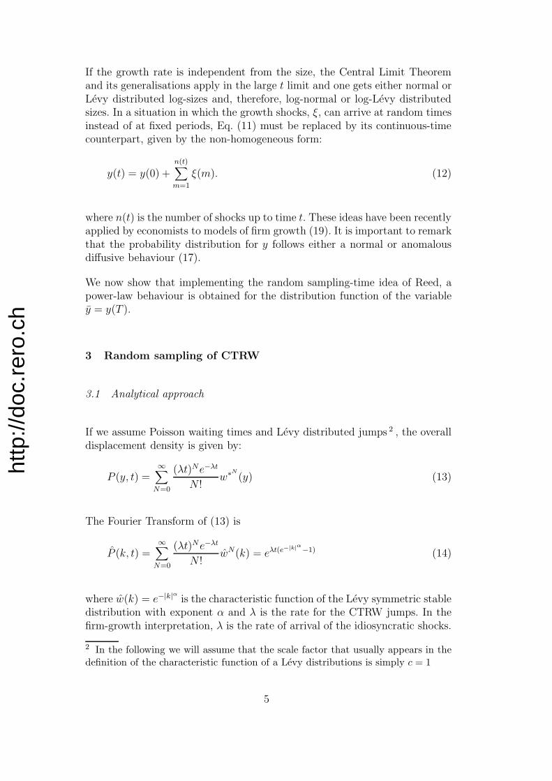
Fig. 1. Tail of the complementary cumulative distribution function (CCDF) for thevariable y for α = 1.1 and α = 1.7. In the two plots the behaviour of y−α is alsoreported. In the two insets, the whole CCDF is plotted. The number N of pointsused for building the CCDF is 107. Values of the parameters in the simulation are:N = 107; Λ = 10−3; λ = 2 ∗ 10−2 (see text for details).

same exponent. In order to check this prediction we performed extensive MonteCarlo simulation. For every simulation we sampled N = 107 points of ourprocess. In Fig. (1) the tail of the complementary cumulative distributionfunction is plotted for two different values of α. In the same plot we reportedalso the straight lines with slope α. In the case α = 1.1, the agreement betweenthe analytical prediction and the Monte Carlo simulation is good. For α = 1.7,the agreement is still satisfactory, but finite-size effects in the simulation arestronger (21).

4 Conclusions

CTRWs are suitable models of asynchronous random processes. For this rea-son, we computed the probability density of a CTRW with exponentially-distributed waiting times and α-Levy-stable distributed jumps, after randomsampling of the evaluation times. Our main result is given in Eq. (18). Itturns out that the tail of the complementary cumulative distribution functionfor the variable y = y(T ) follows a power-law with exponent α equal to theexponent of the jumps. When y has the meaning of log-size of, e.g., a set offirms,y = ln(x) one should notice that the size distribution is no longer strictlypower law, but a logarithmic correction is necessary:

P (x) = P (y)|dy

dx| � 1

|x|[ln(x)]α+1. (21)

7

http

://do

c.re

ro.c

h

It should be noticed that our result entails for this model a super-universalityfor the direct stochastic variable involved, that is β = 1, when x is so largethat the logarithmic correction can be neglected. This analytical result doesnot explain the empirical distribution of firm sizes where an exponent β � 2has been estimated (20). However, it is necessary to be careful when com-paring theoretical results to estimates of power-law exponents, as the latterare delicate (21). It has been shown that a suitable CTRW model can in-deed reproduce various stylised facts of firm growth distributions, but randomsampling in time is not necessary (19).

A possible shortcoming of our model is implicit in the exponential distributionof the sampling times T ; more realistic distributions (albeit with memory) willbe taken into consideration in the future.

Acknowledgements

We are grateful to G. Bottazzi and G. Yaari for useful discussions. E. S. hasbeen partially supported by the Italian MIUR project “Dinamica di altissimafrequenza nei mercati finanziari”.

References

[1] P. Bak, C. Tang, and K. Wiesenfeld, Phys. Rev. Lett., 59, 1987, 381; P.Bak, How Nature Works: The Science of Self-Organised Criticality (Coper-nicus Press, NY, 1996).

[2] W.J. Reed, Econ. Lett., 74, 2001, 15; W.J. Reed, and B.D. Hughes, Phys.Rev. E, 66, 2002, 067103.

[3] M.O. Lorenz, Publications of the American Statistical Association, 9, 1905,209; H.F. Lydall, Econometrica, 27, 1959, 110.

[4] G.K. Zipf, Human Behaviour and the Principle of Least Effort (Addison-Wesley, Cambridge MA, 1949).

[5] B.B. Mandelbrot, J. of Business, 36, 1963, 394.[6] R.N. Mantegna, and H.E. Stanley, Nature, 376, 1995, 46.[7] H. Hinrichsen, and D.E. Wolf, The Physics of Granular Media, (Wiley,

NY, 2004).[8] B.B. Mandelbrot, The Fractal Geometry of Nature, (W.H. Freeman and

Co. NY, 1977); D.W.G. Arthur, J. of the British Astronomical Association,64, 1954, 127.

[9] B. Burlando, J. Theor. Biol., 146, 1990, 161.[10] B. Drossel, and F. Schwabl, Phys. Rev. Lett., 69, 1992, 1629.[11] E. Milotti, ArXiv: physics/0204033; B.B. Mandelbrot, Multifractals and

8

http

://do

c.re

ro.c

h

1/f Noise: Wild Self-Affinity in Physics (1963-1976) (Springer-Verlag,Berlin, 1999).

[12] E. Puppin, Phys. Rev. Lett., 84, 2000, 5415.[13] C.W. Gardiner, Handbook of Stochastic Methods (Springer, Berlin,

1986).[14] E. Scalas, R. Gorenflo, and F. Mainardi, Physica A, 284, 2000, 376 ; F.

Mainardi, M. Raberto, R. Gorenflo, and E. Scalas, Physica A, 287, 2000,468.

[15] R. Gibrat, Les Inegalites Economiques, Application: Aux Inegalites desRichesses, a la Concentration des Entreprises, aux Populations des Villes,aux Statistiques des Familles, etc., d’une Loi Nouvelle, la Loi de l’EffetProportionnel (Librarie du Recueil Sirey, Paris, 1931).

[16] M. Buchanan, Ubiquity: The Science of History (Weidenfeld & Nicholson,London, 2000); T. Lux in: A. Chatterjee, S. Yarlagadda, B.K. Chakrabarti,Eds., Econophysics of Wealth Distribution (Springer, Berlin, 2005).

[17] E. Scalas Physica A, 362, 2006, 225.[18] S. Solomon, in: G. Ballot, G. Weisbuch, Eds., Applications of Simulation

to Social Sciences (Hermes Science Publishing, London, 2000).[19] G.Bottazzi, LEM Working Paper n. 2001-01, Scuola Superiore Sant’Anna

(2001); G.Bottazzi and A.Secchi, Rand Journal of Economics, 37, 2006. G.Bottazzi and A. Secchi, LEM Working Paper n. 2006-18, Scuola SuperioreSant’Anna (2006); G. Bottazzi, G Dosi, and G. Fagiolo, in Breschi, S. andMalerba, F. Eds., Clusters, networks and innovation (Oxford UniversityPress, Oxford, U.K., 2006).

[20] R. Axtell Science, 293, 2001, 1818; E. Gaffeo, M. Gallegati, and A.Palestrini Physica A, 324, 2003, 117; D. Delli Gatti, C. Di Guilmi, E.Gaffeo, G. Giulioni, M. Gallegati, and A. Palestrini, Journal of EconomicBehavior and Organization, 56, 2005, 489.

[21] R. Weron Int. J. Mod. Phys. C, 12, 2001, 209; M.E.J. Newman Contem-porary Physics, 46, 2005, 323.

9