EPJ manuscript No.(will be inserted by the editor)

Discriminating word senses with tourist walks in complexnetworks

Thiago C. Silva1 and Diego R. Amancio2

1 Institute of Mathematics and Computer ScienceUniversity of Sao Paulo, P. O. Box 369, Postal Code 13560-970Sao Carlos, Sao Paulo, Brazil

2 Institute of Physics of Sao CarlosUniversity of Sao Paulo, P. O. Box 369, Postal Code 13560-970Sao Carlos, Sao Paulo, Brazil

Received: date / Revised version: date

Abstract. Patterns of topological arrangement are widely used for both animal and human brains in thelearning process. Nevertheless, automatic learning techniques frequently overlook these patterns. In thispaper, we apply a learning technique based on the structural organization of the data in the attribute spaceto the problem of discriminating the senses of 10 polysemous words. Using two types of characterization ofmeanings, namely semantical and topological approaches, we have observed significative accuracy rates inidentifying the suitable meanings in both techniques. Most importantly, we have found that the character-ization based on the deterministic tourist walk improves the disambiguation process when one compareswith the discrimination achieved with traditional complex networks measurements such as assortativityand clustering coefficient. To our knowledge, this is the first time that such deterministic walk has beenapplied to such a kind of problem. Therefore, our finding suggests that the tourist walk characterizationmay be useful in other related applications.

PACS. 89.75.Hc Networks and genealogical trees – 02.40.Pc General topology – 02.50.-r Probabilitytheory, stochastic processes, and statistics

1 Introduction

The last few years have seen a wave of automatic ap-proaches devoted to processing natural languages [1]. Phys-icists usually study language employing concepts from in-formation theory [2] and other physical concepts [3,4,5,6,7]. More recently, language has been studied from a dif-ferent standpoint as it can be schemed as a complex sys-tem. Since traditional computational linguistic tools canhardly capture long-range information concerning the re-lationships between concepts, researchers have used themethods of complex networks [8] and non-linear systemsto study the overall picture of linguistic phenomena. Ex-amples of language studies from the network standpointinclude applications in machine translation [8,9], extrac-tive summarization [8] and information retrieval. From atheoretical point of view, complex networks have beenused to study patterns of language [10], linguistic evo-lution [11] and to investigate the origin of fundamentalproperties [12], such as the Zipf’s law and word order.Interestingly, one of the most interesting patterns foundwith the study of language as a network refers to the factthat most language networks, even when modeled with

different building rules, exhibit similar features, such asthe so called scale-free and small-world effects [10].

In the current paper, we evaluate the ability of complexnetworks for the Word Sense Disambiguation (WSD) task(i.e., the discrimination of which of the meanings is usedin a given context for a word that has multiple meanings).Traditional approaches make use of contextual attributesof neighboring words to discriminate senses. In such meth-ods, the context of ambiguous words is recognized with thecomputation of corpus-based features such as the part-of-speech of nearby words [1], the grammatical or syntacticalrelations between the word of interest and the other sur-rounding words [13]. A second approach, referred to asknowledge-based paradigm (see e.g. Ref. [14] and refer-ences therein), relies on the analysis of context to infermeaning with the aid of semantic resources. In this case,thesauri [15], ontologies [16], machine machine-readabledictionaries [17] and several others sources of knowledgeresources [13,18] have been useful to provide semantic tipsabout the context of ambiguous words. In recent studies,features extracted from both corpus- and knowledge-basedparadigms have been successfully integrated to yield more

arX

iv:1

306.

3920

v1 [

cs.C

L]

17

Jun

2013

2 Thiago C. Silva, Diego R. Amancio: Discriminating word senses with tourist walks in complex networks

robust discriminative systems [18]. As for the automaticidentification of patterns after the contextual character-ization, pattern recognition techniques such as decisiontrees [19], Naive Bayes [1] and neural networks [20] havebeen employed.

While most traditional approaches disregards the con-nectivity patterns of words, we devised a corpus-basedstrategy that uses topological information extracted fromnetworks modeling the relationship between words in thetextual level [21] and in the attribute space [22]. Initially,the topology of ambiguous words represented as nodesin word adjacency networks was analyzed with a seriesof complex network metrics. Thus, each occurrence of anambiguous word in the text is mapped into an object inthe attribute space. In this space, we applied a hybrid pat-tern recognition which combines semantical and structuralproperties of ambiguous words to perform the discrimina-tion of senses. The results suggest that word senses canbe discriminated because patterns emerge not only in theadjacency networks model but also in the networks arisingfrom the technique devised in the attribute space. Mostimportantly, we show that the introduction of determin-istic tourist walks over the complex network built in theattribute space improves the discrimination of senses incomparison with the same technique based on topologicalmeasurements alone.

2 Methodology

In this section, the methodology applied for discriminat-ing word senses is discussed. The dataset is presented inSection 2.1 and the representation of texts as networks isexplained in Section 2.2. Then the deterministic walk em-ployed for characterizing word senses is discussed in Sec-tion 2.3. We describe traditional classification methods inSection 2.4. Finally, the method devised in the currentpaper is presented in Section 2.5.

2.1 Dataset description

The dataset employed in the WSD task comprises 10 words,which might assume at most four different meanings (seeTable 1). The study of the contextual topological proper-ties of these ambiguous words was carried out on a set of18 books obtained from the Gutenberg1 online repository.The list of books used in the current paper is presented inTable 2.

2.2 Representing texts as complex networks for WSD

Word-sense disambiguation (WSD) refers to the problemof discriminating the meaning used by a polysemous wordin a particular context. The resolution of ambiguities isan essential task in the field of Natural Language Pro-cessing [1] because other tasks (p.e., anaphora resolution,

1 gutenberg.org

Table 1. List of 10 ambiguous words employed in the experi-ments and description of their respective possible senses.

List of words and sensesbear (I) = to endurebear (II) = mammal of the family Ursidaebear (III) = to remember (bear in mind)jam (I) = jellyjam (II) = to compressjust (I) = fairjust (II)= only, simplyjust (III) = at this momentmarch (I) = to trekmarch (II) = third month of the calendarrock (I) = stonerock (II) = to sway, swingrock (III) = name (e.g. Chris Rock)ring (I) = sound of a bellring (II) = circle of metalsave (I) = to rescuesave (II) = to use frugallypresent (I) = nowpresent (II)= to showclose (I) = nearclose (II) = shut, finishnote (I) = to take a noticenote (ii) = brief informal letter

Table 2. List of books (and their respective authors) employedin the experiments aiming at discriminating the meaning ofambiguous words. The year of publication is specified after thetitle of the book.

Title AuthorPride and Prejudice (1813) J. Austen

American Notes (1842) C. DickensCoral Reefs (1842) C. Darwin

A Tale of Two Cities (1859) C. DickensThe Moonstone (1868) W. Collins

Expression of Emotions (1872) C. DarwinA Pair of Blue Eyes (1873) T. HardyJude the Obscure (1895) T. HardyDracula’s Guest (1897) B. Stoker

Uncle Bernac (1897) A. C. DoyleThe Tragedy of the Korosko (1898) A. C. Doyle

The Return of Sherlock Holmes (1903) A. C. DoyleTales of St. Austin’s (1903) P. G. Wodehouse

The Chronicles of Clovis (1911) H. H. MunroA Changed Man (1913) T. Hardy

Beasts and Super Beasts (1914) H. H. MunroThe Wisdom of Father Brown (1914) G. K. Chesterton

My Man Jeeves (1919) P. G. Wodehouse

machine translation and information retrieval) depend onthe accurate discrimination of senses. Traditionally, twoparadigms are employed to address the problem: the deepand the shallow paradigms. While the latter employs sta-tistical techniques to infer contextual information, the for-mer employs knowledge bases, such as dictionaries andthesaurus. In the current paper, we have used the superfi-

Thiago C. Silva, Diego R. Amancio: Discriminating word senses with tourist walks in complex networks 3

RETINA

MIDDLE

EVENT

NEVER

FATIGUE LIFETIME

STONE

FORGET

ROAD

1

1 2 1

61

52

1

1

11

3

Fig. 1. Network obtained from the poem “In the middle ofthe road there was a stone / there was a stone in the middleof the road / there was a stone / in the middle of the roadthere was a stone. / Never should I forget this event / in thelifetime of my fatigued retinas / Never should I forget that inthe middle of the road / there was a stone / there was a stonein the middle of the road / in the middle of the road there wasa stone.” by Carlos Drummond de Andrade.

cial paradigm as it usually yields the best discriminationrates [21].

Two superficial methods were employed in this pa-per. The first method, referred to as semantical approach,is based on the analysis of frequency of nearby words.More specifically, the context surrounding an ambiguousword is mathematically described by the frequency of theirωn closest words. Particularly, we have employed ωn =5, 20, 50. In the second method, referred to as topolog-ical approach, words are represented as nodes [21]. Edgeslinking nodes are created according to the order wordsappear in the text. As such, whenever word i appears im-mediately before word j, the element wij of the matrixW representing the network is incremented by one. Be-fore this step, punctuation marks and stopwords (such asprepositions, articles and other high-frequency words con-veying little semantic meaning) are removed. Then, theremaining words are converted to their canonical form sothat words lexically distinct but semantically related aremapped into the same network node. Specifically, whenmodeling ambiguous words, each of its occurrence is re-garded as as distinct node. An example of the pre-processingsteps taken to process the poem “In the middle of theroad” by Carlos Drummond de Andrade (translation fromPortuguese by Elizabeth Bishop) is given in Table 3. Thegraphical representation of the network originated fromthis poem is provided in Figure 1.

The context surrounding ambiguous words is identi-fied by the recurrence of patterns of connectivity, whichare measured with the following complex networks mea-surements [8]: hierarchical degree, hierarchical clusteringcoefficient, average and variability of the degree of neigh-bors, average shortest path length and betweenness. Fur-

Fig. 2. Illustration of a tourist walk with µ = 1. The greendots represent unvisited sites. The orange and red sites indicatevisited sites, where the first color displays the transient part ofthe tourist walk and the second color, the cycle of the walk.

ther details regarding the topological approach are givenin the Supplementary Information2

2.3 Touristic walks

A tourist walk can be conceptualized as a walker (tourist)aiming at visiting sites (data items) in a d-dimensionalmap, representing the data set. At each discrete time step,the tourist follows a simple deterministic rule: it visitsthe nearest site which has not been visited in the previ-ous µ steps. In other words, the walker performs partiallyself-avoiding deterministic walks over the data set, wherethe self-avoiding factor is limited to the memory windowµ−1. This quantity can be understood as a repulsive forceemanating from the sites in this memory window, whichprevents the walker from visiting them in this interval (re-fractory time). Therefore, it is prohibited that a trajectoryto intersect itself inside this memory window. In spite ofbeing a simple rule, it has been shown that this movementdynamic possesses complex behavior when µ > 1 [23].

Each tourist walk can be decomposed in two terms:(i) the initial transient part of length t and (ii) a cycle(attractor) with period c. Figure 2 shows an illustrationof a tourist walk with µ = 1, i.e., the walker always goesto the nearest neighbor. In this case, one can see that thetransient length is t = 2 and the cycle length c = 8.

2.4 Traditional classification

The traditional bag-of-words [1] technique employed forthe WSD task is exemplified in this section with three low-level algorithms, namely Naive Bayes, kNN and C4.5. For

2 The Supplementary Information is available from https://

dl.dropboxusercontent.com/u/2740286/supEpjb2013.pdf.

4 Thiago C. Silva, Diego R. Amancio: Discriminating word senses with tourist walks in complex networks

Table 3. Pre-processing steps taken to process the poem “In the middle of the road”, by Carlos Drummond de Andrade.Initially punctuation marks and stopwords are taken away from the text. Then the remaining words are mapped into theircanonical forms.

Processing Step Outcome

Original Poem

In the middle of the road there was a stone / there was a stonein the middle of the road there was a stone in the middle of theroad there was a stone. Never should I forget this event / in thelifetime of my fatigued retinas / Never should I forget that inthe middle of the road / there was a stone / there was a stonein the middle of the road / in the middle of the road there wasa stone.

Without stopwordsmiddle road stone stone middle road stone middle road stone neverforget event lifetime fatigued retinas never forget middle road stonestone middle road middle road stone

After Lemmatizationmiddle road stone stone middle road stone middle road stone neverforget event lifetime fatigue retina Never forget middle road stonestone middle road middle road stone

all the three pattern recognition techniques, each contentword surrounding the polysemous word is taken as a singleattribute [1].

2.4.1 Naive Bayes

The Naive Bayes technique is based on the following rule:

Bayesian optimal decision rule : choose sense s′ if thecondition

P (s′|c) > P (sk|c) (1)

holds for each sk 6= s′, where P (sk|c) is the probabilityof the sense sk to occur in the context c.

Usually, the values of P (sk|c) are unknown. Never-theless, they can be recovered straightforwardly from theBayes’s theorem:

P (sk|c) =P (c|sk)

P (c)P (sk). (2)

P (sk) is referred to as a priori probability of sk, i.e., theprobability of sk occur in any context. The evidence con-cerning the context is given by the term P (c|sk). Becausewe are tackling an instantiation of a discrimination task,P (c) can be disregard for it is remains constant for eachsense sk. As such, the most likely sense s′ is given by:

s′ = arg maxsk

P (sk|c)

= arg maxsk

P (c|sk)

P (c)P (sk)

= arg maxsk

P (c|sk)P (sk)

= arg maxsk

[logP (c|sk) + logP (sk)]. (3)

Upon employing the hypothesis of attribute independenceand considering that a neighbor word vj represents thecontext, i.e. c = vj |vj ∈ c, consider the following as-sumption:

Naive Bayes hypothesis :

P (c|sk) = P (vj |vj ∈ c|sk =∏vj∈c

P (vj |sk). (4)

Note that if the Naive Bayes hypothesis is assumed to betrue all the organization of the contextual words is disre-garded. In addition, due to the independence assumption,the presence of an specific word in the context does not af-fect the probability of occurrence of other words. Finally,the most likely sense of the polysemous word is computedas:

s′ = arg maxsk

[logP (sk) +∑vj∈c

logP (vj |sk)]. (5)

In order to illustrate the process of deciding the correctsense of an ambiguous word with the Naive Bayes tech-nique, consider Figure 3. The position of each circle rep-resents the proximity of a given word vj to one of thetwo senses: s =“red” or s =“blue”. Since both senses oc-cur with the same frequency the effective term accountingfor the decision is logP (vj |sk) in equation 5. In the cur-rent paper, the likelihood P (vj |sk) is estimated with theParzen windowing strategy [24]. The decision boundariesare then established according to equation 5. For example,any new instance lying in the interval between -0.19 and0.00 will be classified as s′ =“blue” because this sense isthe most likely sense in that region. In the same way, theinterval lying between 0.00 and 0.18 is governed by the“red” sense because P (vj |“red”) > P (vj |“blue”) in thisparticular interval.

2.4.2 k-nearest neighbors (kNN)

In this technique, each sense s of a given ambiguous wordis attributed according to a voting process performed overthe set of the k nearest neighbors (computed accordingto a similarity measure) comprising the instances labeledpreviously. If most of the k nearest neighbors of the am-biguous word were labeled with sense s′, then sense s′ is at-tributed to the word. To illustrate how the algorithm per-forms the classification, consider Figure 4. Suppose that

Thiago C. Silva, Diego R. Amancio: Discriminating word senses with tourist walks in complex networks 5

RED BLUEBLUE

BLUE

-0.8 -0.4 0.0 0.4 0.8

MEASUREMENT

PROBABILITY

RED

RED

BLUE

BLUE

Fig. 3. Example of decision based on the Naive Bayes al-gorithm. Any word satisfying the condition P (vj |“red”) >P (vj |“blue”) will be classified as s′ =“red”. Analogously,P (vj |“blue”) > P (vj |“red”) determines the boundaries of the“blue” sense decision region.

1.0 1.5 2.0 2.5 3.0 3.5 4.02.0

2.5

3.0

3.5

4.0

4.5

5.0

5.5

6.0

MEASUREMENT X

ME

AS

UR

EM

EN

T Y

Fig. 4. Example of classification with the k-nearest neighbortechnique. Note that the decision relies on a voting process per-formed over the k of nearest neighbors of the ambiguous word,which is represent by the green square. In the experiments weemployed k = 1 along with the Euclidean distance.

we aim at classifying the sense of an polysemous wordillustrated by the green square in Figure 4. If the deci-sion is taken with k = 5 (see the innermost dotted circle),the correct sense would be s′ =“red” because four out ofthe five nearest neighbors belong to the “red” class. Whenthe decision is performed with k = 13 (see the central dot-ted circle) the majority class is the blue one. As a result,s′ =“blue” is the sense associated. In a similar fashion,when k = 19 (see the outermost dotted circle) the senseassociated to the word remains s′ =“blue”.

f > 02

f > 03

s1

s2

s3

f > 01

YES

NO

YES

YES

NO

NO

s1

Fig. 5. Example of decision tree employed to decide the cor-rect sense of an ambiguous word, described by the followingattributes: f1 = −0.23, f2 = +0.29 and f3 = +0.38. The firsttest leads to the edge labeled as “NO” (because f1 > 0) andthe second test leads to the edge “YES” (because f3 > 0).Therefore, the sense s3 is associated to the ambiguous word.

2.4.3 Decision trees

The decision tree algorithm employed in the current paperis the so called C4.5 [25]. The tree used for the decisioncomprises internal and leaf nodes, where the former repre-sent attributes and the latter represent classes (in our case,word senses). Edges represent conditional clauses, such as“IF (attribute ≥ threshold)” or “IF (attribute ≤ thresh-old)”. To classify an unknown instance, one walks on thetree following the rules applied to the attribute related tothe current internal node until one reaches a leaf node.At this point, the class assigned is the class stored in theleaf node. To construct a decision tree, the algorithm C4.5chooses an attribute fi and a threshold L that best sep-arates the dataset [25]. In this case, the criterion used todistinguish items is the information gain [24], which rep-resents the difference in entropy H before and after usingthe attribute to separate the data. More specifically, theinformation gain related to the attribute fi in the trainingset [22] Str is given by:

Ω(Str, fi) = H(Str)−H(Str|fi). (6)

Thus, the attribute with largest information gain receivesthe highest priority to perform the discrimination of senses.The process is reiterated recursively for the two childrennodes of the current node. When separation is complete,i.e. all instances resulting from the separation belongs toa unique class, the process stops and a leaf node is createdto store the corresponding class. The classification processis exemplified in Figure 5. Further details regarding thismethod is provided in Ref. [25].

6 Thiago C. Silva, Diego R. Amancio: Discriminating word senses with tourist walks in complex networks

2.5 Network-based classification

In a typical supervised data classification task, a dataset X is decomposed into two disjoint sets: the trainingset Xtraining, where the labels yi ∈ L = L1, . . . , Lnare known, and the test set Xtest, in which the labelsare unknown. Each instance of Xtraining or Xtest is a d-dimensional vector-based data item [26,27]. Usually, thegeneralization power of the classifier is quantified by mea-suring the accuracy rate achieved when it is applied to thetest set. The training set is used in the training phase toinduce the hypothesis of the classifier, while the test set isutilized in the classification phase to predict new unseeninstances. In the following, these two phases are discussed.

In the training phase, the data in the training set aremapped into a graph G using a network formation tech-nique g : Xtraining 7→ G = 〈V,E〉, where V = 1, . . . , V is the set of vertices and E is the set of edges. Each vertexin V represents a training instance in Xtraining. As it willbe described later, the pattern formation of the classes willbe extracted by using the complex topological features ofthis networked representation.

The edges in E are created using a combination ofthe εr and the k-nearest neighbors (κNN) graph forma-tion techniques. In the original versions, the εr techniquecreates a link between two vertices if they are within adistance ε, while the κNN sets up a link between verticesi and j if i is one of the k nearest neighbors of j or viceversa. Both approaches have their limitations when spar-sity or density is a concern. For sparse regions, the κNNforces a vertex to connect to its k nearest vertices, evenif they are far apart. In this scenario, one can say thatthe neighborhood of this vertex would contain dissimilarpoints. Equivalently, improper ε values could result in dis-connected components, sub-graphs, or isolated singletonvertices.

The network is constructed using these two traditionalgraph formation techniques in a combined form. The neigh-borhood of a vertex xi is given by N(xi) = εr(xi, yxi

),if |εr(xi, yxi

| > k. Otherwise, N(xi) = κ(xi, yxi), where

yxidenotes the class label of the training instance xi,

εr(xi, yxi) returns the set xj , j ∈ V : d(xi, xj) < ε∧yxi

=yxj, and κ(xi, yxi

) returns the set containing the k near-est vertices of the same class as xi. Note that the εr tech-nique is used for dense regions (|εr(xi)| > k), while theκNN is employed for sparse regions. With this mecha-nism, it is expected that each class will have a uniqueand single graph component. For example, Fig. 6 displaysa schematic of how the network looks like for a three-classproblem when the training phase has been completed. Onecan see that each class holds a representative component.

In the classification phase, the unlabeled data itemsin the Xtest are presented to the classifier one by one. Incontrast to the training phase, the class labels of the testinstances are unknown. This test instance is inserted alsousing a mixture of the ε-radius and κNN. In this case,the labels are not taken into consideration. Once the dataitem is inserted, each class analyzes, in isolation, its im-pact on the respective class component using the complextopological features of it. In the high level model, each

ℊc1

ℊc2

ℊc3

Fig. 6. Schematic of the constructed network. At the end ofthe training phase, each class is represented by a graph compo-nent. In the classification phase, a new test instance (yellow or“square-shaped” data) is temporarily inserted into the graph.

class retains an isolated graph component. Each of thesecomponents calculate the changes that occur in its pat-tern formation with the insertion of this test instance. Ifslight or no changes occur, then it is said that the test in-stance is in compliance with that class pattern. As a result,the high level classifier yields a great membership valuefor that test instance on that class. Conversely, if thesechanges dramatically modify the class pattern, then thehigh level classifier produces a small membership value onthat class. These changes are quantified via network mea-sures, each of which numerically translating the organiza-tion of the component from a local to global fashion. Forthis end, the touristic walks are employed in a novel man-ner. Again, in Fig. 6, a test instance denoted by the yellowor “square-shaped” data item is temporarily inserted intothe network (dashed lines). Due to its insertion, the class

components become altered: G′

C1, G′

C2, and G′

C3. It may

occur that some class components do not share any linkswith this test instance. In the figure, this happens withG′

C3. In this case, we say that test instance do not comply

to the pattern formation of the class component. For thecomponents that share at least a link (G′

C1and G′

C2), each

of it calculates considers only the edges of the test instancethat are linked to it in order to measure the compliance.For instance, when we check the compliance of the testinstance with the component G′

C1, the connections from

the test instance to the component G′

C2are ignored, and

vice versa.

Simultaneously to the prediction yielded by the highlevel classifier, a low level classifier also predicts the mem-bership of the same test instance. The way it predictsdepends on the choice of the low level classifier. In theend, the predictions produced by both classifiers are com-bined via a linear combination to derive the prediction ofthe high level framework (meta-learning). Once the testinstance gets classified, it is either discarded or incorpo-

Thiago C. Silva, Diego R. Amancio: Discriminating word senses with tourist walks in complex networks 7

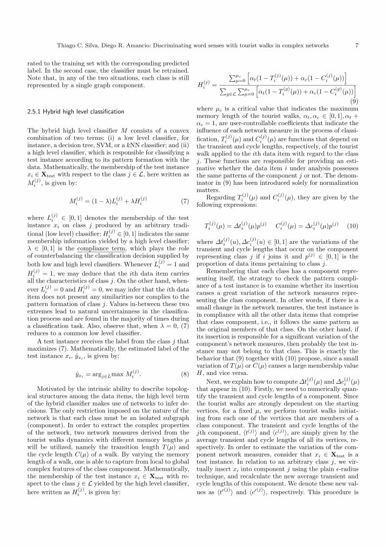
rated to the training set with the corresponding predictedlabel. In the second case, the classifier must be retrained.Note that, in any of the two situations, each class is stillrepresented by a single graph component.

2.5.1 Hybrid high level classification

The hybrid high level classifier M consists of a convexcombination of two terms: (i) a low level classifier, forinstance, a decision tree, SVM, or a kNN classifier; and (ii)a high level classifier, which is responsible for classifying atest instance according to its pattern formation with thedata. Mathematically, the membership of the test instancexi ∈ Xtest with respect to the class j ∈ L, here written as

M(j)i , is given by:

M(j)i = (1− λ)L

(j)i + λH

(j)i (7)

where L(j)i ∈ [0, 1] denotes the membership of the test

instance xi on class j produced by an arbitrary tradi-

tional (low level) classifier; H(j)i ∈ [0, 1] indicates the same

membership information yielded by a high level classifier;λ ∈ [0, 1] is the compliance term, which plays the roleof counterbalancing the classification decision supplied by

both low and high level classifiers. Whenever L(j)i = 1 and

H(j)i = 1, we may deduce that the ith data item carries

all the characteristics of class j. On the other hand, when-

ever L(j)i = 0 and H

(j)i = 0, we may infer that the ith data

item does not present any similarities nor complies to thepattern formation of class j. Values in-between these twoextremes lead to natural uncertainness in the classifica-tion process and are found in the majority of times duringa classification task. Also, observe that, when λ = 0, (7)reduces to a common low level classifier.

A test instance receives the label from the class j thatmaximizes (7). Mathematically, the estimated label of thetest instance xi, yxi

, is given by:

yxi= argj∈Lmax M

(j)i . (8)

Motivated by the intrinsic ability to describe topolog-ical structures among the data items, the high level termof the hybrid classifier makes use of networks to infer de-cisions. The only restriction imposed on the nature of thenetwork is that each class must be an isolated subgraph(component). In order to extract the complex propertiesof the network, two network measures derived from thetourist walks dynamics with different memory lengths µwill be utilized, namely the transition length T (µ) andthe cycle length C(µ) of a walk. By varying the memorylength of a walk, one is able to capture from local to globalcomplex features of the class component. Mathematically,the membership of the test instance xi ∈ Xtest with re-spect to the class j ∈ L yielded by the high level classifier,

here written as H(j)i , is given by:

H(j)i =

∑µc

µ=0

[αt(1− T (j)

i (µ)) + αc(1− C(j)i (µ))

]∑g∈L

∑µc

µ=0

[αt(1− T (g)

i (µ)) + αc(1− C(g)i (µ))

](9)

where µc is a critical value that indicates the maximummemory length of the tourist walks, αt, αc ∈ [0, 1], αt +αc = 1, are user-controllable coefficients that indicate theinfluence of each network measure in the process of classi-

fication, T(j)i (µ) and C

(j)i (µ) are functions that depend on

the transient and cycle lengths, respectively, of the touristwalk applied to the ith data item with regard to the classj. These functions are responsible for providing an esti-mative whether the data item i under analysis possessesthe same patterns of the component j or not. The denom-inator in (9) has been introduced solely for normalizationmatters.

Regarding T(j)i (µ) and C

(j)i (µ), they are given by the

following expressions:

T(j)i (µ) = ∆t

(j)i (µ)p(j) C

(j)i (µ) = ∆c

(j)i (µ)p(j) (10)

where ∆t(j)i (u), ∆c

(j)i (u) ∈ [0, 1] are the variations of the

transient and cycle lengths that occur on the componentrepresenting class j if i joins it and p(j) ∈ [0, 1] is theproportion of data items pertaining to class j.

Remembering that each class has a component repre-senting itself, the strategy to check the pattern compli-ance of a test instance is to examine whether its insertioncauses a great variation of the network measures repre-senting the class component. In other words, if there is asmall change in the network measures, the test instance isin compliance with all the other data items that comprisethat class component, i.e., it follows the same pattern asthe original members of that class. On the other hand, ifits insertion is responsible for a significant variation of thecomponent’s network measures, then probably the test in-stance may not belong to that class. This is exactly thebehavior that (9) together with (10) propose, since a smallvariation of T (µ) or C(µ) causes a large membership valueH, and vice versa.

Next, we explain how to compute∆t(j)i (µ) and∆c

(j)i (µ)

that appear in (10). Firstly, we need to numerically quan-tify the transient and cycle lengths of a component. Sincethe tourist walks are strongly dependent on the startingvertices, for a fixed µ, we perform tourist walks initiat-ing from each one of the vertices that are members of aclass component. The transient and cycle lengths of thejth component, 〈t(j)〉 and 〈c(j)〉, are simply given by theaverage transient and cycle lengths of all its vertices, re-spectively. In order to estimate the variation of the com-ponent network measures, consider that xi ∈ Xtest is atest instance. In relation to an arbitrary class j, we vir-tually insert xi into component j using the plain ε-radiustechnique, and recalculate the new average transient andcycle lengths of this component. We denote these new val-

ues as 〈t′(j)〉 and 〈c′(j)〉, respectively. This procedure is

8 Thiago C. Silva, Diego R. Amancio: Discriminating word senses with tourist walks in complex networks

performed for all classes j ∈ L. It may occur that someclasses u ∈ L will not share any connections with the

test instance xi. Using this approach, 〈t(k)〉 = 〈t′(k)〉 and

〈c(k)〉 = 〈c′(k)〉, which is undesirable, since this configura-tion would state that xi complies perfectly with class u. Inorder to overcome this problem, a simple post-processingis necessary: For all components u ∈ L that do not share

at least 1 link with xi, we deliberately set 〈t′(j)〉 and 〈c′(j)〉to a high value. This high value must be greater than thelargest variation that occurs in a component which sharesa link with the data item under analysis. One may inter-pret this post-processing as a way to state that xi do notshare any pattern formation with class u, since it is noteven connected to it.

With all this information at hand, we are able to cal-

culate ∆t(j)i (µ) and ∆c

(j)i (µ),∀j ∈ L, as follows:

∆t(j)i (µ) =

|〈t′(j)〉 − 〈t(j)〉|∑u∈L |〈t′

(u)〉 − 〈t(u)〉|(11)

∆c(j)i (µ) =

|〈c′(j)〉 − 〈c(j)〉|∑u∈L |〈c′

(u)〉 − 〈c(u)〉|(12)

The network-based high level classifier quantifies thevariations of the transient and cycle lengths of touristwalks with limited memory µ that occur in the class com-ponents when a test instance artificially joins each of themin isolation. According to (9), this procedure is performedfor several values of the memory length µ, ranging from 0(memoryless) to a critical value µc. This is done in orderto capture complex patterns of each of the representativeclass components in a local to global fashion. When µ issmall, the walks tend to possess a small transient and cy-cle parts, so that the walker does not wander far awayfrom the starting vertex. In this way, the walking mech-anism is responsible for capturing the local structures ofthe class component. On the other hand, when µ increases,the walker is compelled to venture deep into the compo-nent, possibly very far away from its starting vertex. Inthis case, the walking process is responsible for capturingthe global features of the component. In summary, thefundamental idea of the high level classifier is to make useof a mixture of local and global features of the class com-ponents by means of a combination of tourist walks withdifferent values of µ.

3 Results and discussion

First, the methodology is applied to an artificial databasein order to better understand its functionality. Afterwards,the WSD problem is analyzed. The discussion of the ob-served results is given below.

3.1 High Level Applied to a Toy Database

In order to better understand the dynamics of the model,consider the toy data set depicted in Fig. 7(a), where there

are two classes: the orange or “square” (14 vertices) andthe blue or “circle” (20 vertices) classes. This exampleserves as a gist of how the hybrid classifier draws its deci-sions. In the training and classification phases, we employκ = 3 and ε = 0.02 for the network construction. Thefuzzy SVM [28] with RBF kernel (C = 40 and γ = 22) isadopted for the low level classifier. By inspection of thefigure, the orange or “square” class displays a well-definedpattern: a pyramidal structure, whereas the blue or “cir-cle” class does not indicate any well-established patterns.Here, the goal is to classify the green or “triangle” dataitem using only the information of the training set. Fig-ures 7(a), 7(b), and 7(c) exhibit the decision boundariesof the two classes when λ = 0, λ = 0.5, and λ = 0.8, re-spectively. When λ = 0, only the SVM prediction is usedby the hybrid technique. In this case, one can see thatthe triangle-shaped data item is not correctly classified.Notice that the decision boundaries are pushed near theblue or “circle” class by virtue of the large amount of blueor “square” items in the vicinity. Now, when λ = 0.5, theSVM and the high level classifier predictions are utilizedin the same intensity. In this situation, the decision bound-aries are dragged toward the orange or “square” class, be-cause of the strong pattern that it exhibits. We can thinkthis phenomenon as being a clash between the two deci-sion boundaries: as λ increases, the more structured classtends to possess more decision power, and, consequently,is able to reduce the effective area of the competing class.For example, when λ = 0.8, the organizational features ofthe orange or “square” class are so salient that its effectivearea invades the high density region of the blue or “circle”class. In the two former cases, the hybrid high level tech-nique can successfully classify the triangle-shaped dataitem.

3.2 High-Level applied to word sense disambiguation

The high-level technique was applied to the problem ofdiscriminating senses of 10 polysemous words. We usedthe database described in Section 2.1, which is availableonline3. For the characterization of senses, two paradigmswere employed: the traditional based on the recurrence ofneighbors (see Table 4) and the one based on the struc-ture of the word adjacency network (see Table 5). In bothcases, we can see that the best results occur when λ > 0.This means that structural patterns in the attribute spaceemerge both on the semantical and topological character-ization. In particular, the strongest dependence (i.e., thelowest p-values) between word senses and structural orga-nization in the word adjacency networks was observed forthe words rock and close. For the semantic approach, thestrongest dependence was found for the words ring androck.

One can wonder the reason behind retrieving a walkwith such complex behavior to solve this kind of problem

3 The database of features extracted from the set of am-biguous words is available from dl.dropbox.com/u/2740286/

database_words.zip

Thiago C. Silva, Diego R. Amancio: Discriminating word senses with tourist walks in complex networks 9

node2

node8

node4

node16

node15

node13

node10

node14

node11

node21

node18

node19

node32

node9

node30

node6

node7

node31node29

node34

node25

node24node23

node35

node22

node27node26 node28

node5

node1

node0

node17

node2

node8

node4

node16

node15

node13

node10

node14

node11

node21

node18

node19

node32

node9

node30

node6

node7

node31node29

node34

node25

node24node23

node35

node22

node27node26 node28

node5

node1

node0

node17

node2

node8

node4

node16

node15

node13

node10

node14

node11

node21

node18

node19

node32

node9

node30

node6

node7

node31node29

node34

node25

node24node23

node35

node22

node27node26 node28

node5

node1

node0

node17

a b c

Fig. 7. An artificial data set containing a structured and a non-structured class. The behavior of the decision boundaries variesas λ increases. Decision boundaries correspond to (a) λ = 0; (b) λ = 0.5; and (c) λ = 0.8.

Table 4. Semantic approach for discriminating senses of ambiguous words. Senses were characterized according to frequencyof the n = 5 neighbors of the ambiguous word [21] and the discrimination of senses was performed with low (kNN, C4.5 andBayes) and high level classifiers. Acc. Rate represents the accuracy rate obtained with an evaluation based on the 10-fold cross-validation technique [35]. The p-value refers to the likelihood of obtaining the same accuracy rate with an random classifier (seeRef. [21] for details). Note that the high level technique always outperforms the traditional low level classification.

Approach Low Level Classification High Level ClassificationWord Algorithm Acc. Rate p-value Acc. Rate p-value Best λ

kNN 79.5 % 4.6× 10−1 83.3 % 1.8× 10−1 0.20save C4.5 78.9 % 5.6× 10−1 85.8 % 7.3× 10−2 0.30

Bayes 76.6 % 7.5× 10−1 83.3 % 1.8× 10−1 0.35

kNN 82.6 % 1.3× 10−1 87.9 % 7.6× 10−3 0.25note C4.5 79.5 % 3.7× 10−1 85.0 % 5.3× 10−2 0.25

Bayes 78.3 % 4.6× 10−1 85.0 % 5.3× 10−2 0.30

kNN 82.8 % 8.1× 10−3 90.5 % 3.3× 10−4 0.35march C4.5 82.8 % 8.1× 10−3 90.5 % 3.3× 10−4 0.30

Bayes 62.5 % 4.2× 10−1 71.4 % 1.5× 10−1 0.30

kNN 62.9 % 7.0× 10−1 68.8 % 1.0× 10−2 0.20present C4.5 57.0 % 9.8× 10−1 60.1 % 8.9× 10−1 0.10

Bayes 60.2 % 8.9× 10−1 64.4 % 5.3× 10−1 0.15

kNN 76.5 % 1.6× 10−2 90.0 % 4.6× 10−2 0.40jam C4.5 76.5 % 4.6× 10−2 90.0 % 4.6× 10−2 0.45

Bayes 90.0 % 4.6× 10−2 90.0 % 4.6× 10−2 0.35

kNN 80.7 % 7.2× 10−3 86.4 % 3.4× 10−5 0.25ring C4.5 84.4 % 2.8× 10−4 89.8 % 7.0× 10−7 0.20

Bayes 83.5 % 7.0× 10−4 87.0 % 3.4× 10−5 0.15

kNN 47.4 % 1.1× 10−1 59.1 % 6.8× 10−5 0.50just C4.5 38.0 % 8.0× 10−1 48.5 % 5.5× 10−2 0.40

Bayes 52.6 % 5.9× 10−3 63.3 % 1.0× 10−6 0.45

kNN 48.0 % 6.2× 10−1 53.7 % 2.3× 10−1 0.20bear C4.5 62.0 % 8.0× 10−3 65.4 % 1.1× 10−3 0.15

Bayes 48.0 % 6.2× 10−1 54.9 % 1.3× 10−1 0.30

kNN 69.7 % 3.6× 10−4 69.7 % 3.6× 10−4 0.00rock C4.5 68.5 % 7.4× 10−4 70.0 % 1.7× 10−4 0.10

Bayes 77.5 % 1.0× 10−7 77.5 % 1.0× 10−7 0.00

kNN 64.8 % 9.1× 10−1 70.5 % 2.1× 10−1 0.25close C4.5 71.9 % 1.0× 10−2 76.1 % 1.7× 10−3 0.15

Bayes 75.3 % 3.9× 10−3 80.0 % 3.7× 10−6 0.15

in detriment to simply using well-known complex networkmeasurements, such as assortativity, clustering coefficient,or average degree. This was devised on account of the waythat the tourist walks artlessly supply structural informa-tion of the network in a local to global fashion by simpleranging the size of the memory of the tourist. As we in-crement the memory of the tourist, it gradually capturesmore global information of the network, since the cycleand transient lengths tend to vary more in relation to

small values of µ. In contrast to that, each complex net-work measurement captures, in a static manner, a specificnetwork’s characteristic. For instance, the degree strictlycaptures local organization of each vertex; the clusteringcoefficient captures quasi-local relations, since it investi-gates the neighborhood’s structure, in search of triangles;and the assortativity aims at exclusively unveiling globalinformation of each network component. Therefore, theidea of gradually capturing the network characteristics of

10 Thiago C. Silva, Diego R. Amancio: Discriminating word senses with tourist walks in complex networks

Table 5. Structural approach for discriminating senses of ambiguous words. Senses were characterized according to topologicalCN measurements [21] and the discrimination of senses was performed with low (kNN, C4.5 and Bayes) and high level classifiers.Note that the high level technique always outperforms the traditional low level classification.

Approach Low Level Low Level Classification High Level ClassificationWord Algorithm Acc. Rate p-value Acc. Rate p-value Best λ

kNN 87.6 % 2.1× 10−2 90.9 % 1.6× 10−3 0.15save C4.5 79.8 % 4.5× 10−1 86.0 % 4.1× 10−2 0.25

Bayes 83.1 % 1.8× 10−1 86.0 % 4.1× 10−2 0.10

kNN 84.5 % 2.6× 10−1 86.1 % 1.1× 10−1 0.10note C4.5 78.4 % 8.2× 10−1 81.4 % 5.6× 10−1 0.10

Bayes 78.4 % 8.2× 10−1 81.4 % 5.6× 10−1 0.10

kNN 87.0 % 1.9× 10−3 89.3 % 3.3× 10−4 0.15march C4.5 60.9 % 4.2× 10−1 73.4 % 6.8× 10−2 0.40

Bayes 73.9 % 6.8× 10−2 77.9 % 2.6× 10−2 0.25

kNN 71.1 % 2.2× 10−3 73.6 % 2.7× 10−3 0.30present C4.5 64.7 % 4.7× 10−1 67.8 % 1.7× 10−1 0.25

Bayes 73.9 % 1.7× 10−3 77.8 % 2.8× 10−5 0.40

kNN 100.0 % 6.0× 10−3 100.0 % 6.0× 10−3 0.00jam C4.5 80.0 % 1.7× 10−1 85.6 % 4.6× 10−2 0.20

Bayes 90.0 % 4.6× 10−2 92.8 % 4.6× 10−2 0.10

kNN 84.6 % 2.8× 10−4 92.4 % 3.3× 10−8 0.35ring C4.5 71.4 % 2.8× 10−1 78.3 % 2.5× 10−1 0.30

Bayes 69.2 % 4.6× 10−1 75.7 % 6.9× 10−2 0.25

kNN 51.3 % 1.6× 10−2 60.0 % 3.1× 10−5 0.45just C4.5 47.0 % 1.1× 10−1 55.8 % 1.0× 10−3 0.35

Bayes 46.2 % 1.5× 10−1 53.3 % 5.9× 10−3 0.30

kNN 62.0 % 8.0× 10−3 67.2 % 2.6× 10−4 0.25bear C4.5 62.0 % 8.0× 10−3 68.9 % 1.1× 10−4 0.30

Bayes 60.9 % 1.4× 10−2 67.0 % 2.6× 10−4 0.25

kNN 78.4 % 3.2× 10−8 82.1 % 1.9× 10−10 0.15rock C4.5 79.3 % 9.7× 10−9 84.5 % 2.3× 10−12 0.15

Bayes 70.3 % 1.8× 10−4 73.3 % 1.5× 10−5 0.10

kNN 72.2 % 8.0× 10−2 81.8 % 6.0× 10−8 0.35close C4.5 68.7 % 4.7× 10−1 80.1 % 1.9× 10−6 0.40

Bayes 68.7 % 4.7× 10−1 79.4 % 6.8× 10−6 0.35

the network from a local to global fashion ceases to existwhen one utilizes pre-made network measurements. As aresult, this makes room for an evident gap that links themeasurements that analyze completely local and globalpeculiarities of the network. One could argue that othernew measurements could be plugged into the high order oflearning term of the classifier. This would solve the prob-lem at the cost of creating unnecessary complexity to themodel, as well as spending a great amount of time to de-vise these specific network measurements. As we can see,when we utilize the tourist walks with varying memorylengths, this gap is filled in a concise and clear manner byjust incrementing µ. This effect is illustrated in Figures 8and 9 for the words “close” and “present”, respectively4.As one can observe, in the WSD task a distinct behav-ior arises both in the evolution of the t and c for specificword senses. In the case of the word “close”, the transientlengths discriminate the two possible senses for a memorylength µ ≥ 6. With regard to the word “present”, a dis-crimination of senses occurs for µ ≥ 5. The dependence of

4 The relationship between t and c with µ for the other wordsis presented in the SI.

the cycle length c with µ also seems to be sense-specific.Remarkably, distinct senses are characterized by distincttimes for c to reach the steady state, i.e., the state wherethere is no variation in response to the increase of µ. Theseresults suggests that the complexity of each componentrepresenting a word sense can be grasped with the intro-duction of further memory lengths and then employed toimprove the discrimination of polysemous words.

4 Conclusion

Patterns of structural organization are often used in theprocess of human learning. Nevertheless, automatic pat-tern recognition techniques oftentimes disregard these pat-terns. For this reason, in the current study, we have ap-plied a recognition technique based on organizational pat-terns specifically to the problem of word senses recognitionin a given context. Through the semantic and topologicalcharacterization of the words, we have noticed that thediscrimination is improved with the high-level technique.These results suggest that there are organizational pat-terns in the resulting space, regardless of the paradigm em-

Thiago C. Silva, Diego R. Amancio: Discriminating word senses with tourist walks in complex networks 11

Memory Length (μ)

Memory Length (μ)

Sense “near”

Sense “finish”

0 2 4 6 8 10 12 14 16 18 200

5

10

15

20Tra

ns

ien

t L

en

gth

(t)

Sense “near”

Sense “finish”

0 2 4 6 8 10 12 14 16 18 200

1

2

3

4

5

6

Cy

cle

Le

ng

th (

c)

Fig. 8. Analysis of variability of t and c with µ for two senses of the word “close”. t and c are useful to discriminate senses forµ ≥ 6. The time to reach the steady state (bottom panel) suggests that distinct senses are characterized by distinct patterns ofcomplexity.

Memory Length (μ)

0 5 10 15 20 25 300

5

10

15

20

Memory Length (μ)

Tra

nsie

nt

Len

gth

(t)

Sense “now”

Sense “to show”

0 5 10 15 20 25 300

1

2

3

4

5

6

7

Cycle

Len

gth

(c)

Fig. 9. Analysis of variability of t and c with µ for two senses of the word “present”. t and c are useful to discriminate senses forµ ≥ 4 and µ ≥ 6, respectively. The time to reach the steady state (bottom panel) suggests that distinct senses are characterizedby distinct patterns of complexity.

12 Thiago C. Silva, Diego R. Amancio: Discriminating word senses with tourist walks in complex networks

ployed to characterize the word senses. Most importantly,we have found that the characterization via touristic walksyielded better discrimination rates when compared to thecharacterization based only in complex networks measure-ments, such as clustering coefficient and betweenness [21].A reason for this important phenomenon was discussed.This finding also suggests that this kind of characteriza-tion may be useful in other related applications. At last,we have found that both syntactic and semantic factorsplay a key role in identifying the meaning of the words, forthe best approach (semantical or topological) dependedfrom word to word.

Future works could study how one can automaticallychoose the best value for the compliance term. We alsointend to apply the same methodology devised here withothers classifying schemes [29,30] and in other classifica-tion tasks [31], such as the problems of disambiguatingnames in citation networks [32,33,34].

Acknowledgments

TCS (2009/12329-1) and DRA (2010/00927-9) acknowl-edge the financial support from FAPESP.

References

1. Manning C D and Schtze H 1999 Foundations of StatisticalNatural Language Processing (MIT Press)

2. Shannon C E Bell System Technical Journal 27 (1948) 3793. Carpena P, Bernaola-Galvn P, Hackenberg M, Coronado A.

V. and Oliver J L Phys. Rev. E (2009) 79 0351024. Ortuo M, Carpena P, Bernaola-Galvn P, Muoz E and So-

moza A M Europhys. Lett. (2009) 57 7595. Alis C M and Lim M T The European Physical Journal B

(2012) 85, 397.6. Castell X, Baronchelli A and Loreto V The European Phys-

ical Journal B (2009) 71 557-564.7. Herrera J P and Pury P A The European Physical Journal

B (2008) 63 135-146.8. Costa L F, Rodrigues F A, Travieso G and Villas Boas P R

Advances in Physics (2007) 99. Amancio D R, Oliveira Jr. O N. and Costa L F Physica A

(2012) 391 440610. Masucci A P and Rodgers G J Phys. Rev. E (2006) 74

02610211. Amancio D R, Oliveira Jr O N and Costa L F New Journal

of Physics (2012) 14 04302912. Ferrer i Cancho R and Sole R V Procs. Natl. Acad. Sci.

USA (2003) 100 78813. Navigli R ACM Comput. Surv. (2009) 41 214. Lesk M Proceedings of the 1986 SIGDOC Conference, As-

sociation for Computing Machinery (1986) 2426.15. Roget P M 1911 Rogets International Thesaurus

(Cromwell) 1st ed. , New York, NY16. G A Miller Communications of the ACM (1995) 38 11 39-

41.17. Soanes C and Stevenson 2003 Oxford Dictionary of English

(Oxford University Press)18. Montoyo A, Palomar M, Rigau G and Suarez A Journal

Of Artificial Intelligence Research (2005) 23 299-330

19. Rokach L. and Maimon O. Z. 2008 Data mining with deci-sion trees: theroy and applications (World Scientific Pub CoInc)

20. Haykin S O 2008 Neural networks and learning machines(Prentice Hall)

21. Amancio D R, Oliveira Jr. O N and Costa L F EurophysicsLetters (2012) 98 18002

22. Silva T C and Zhao L IEEE Transactions on Neural Net-works and Learning Systems (2012) 23 6

23. Lima G F, Martinez A S and Kinouchi O Phy. Rev. Lett.87 (2001) 010603

24. Duda R O, Hart P E and Stork D G 2000 Pattern classi-fication (Wiley-Interscience)

25. Quinlan J R 1992 C4.5: Programs for machine learning(Morgan Kaufmann)

26. Silva T C and Zhao L IEEE Transactions on Neural Net-works and Learning Systems (2012) 23 3

27. Silva T C and Zhao L IEEE Transactions on Neural Net-works and Learning Systems (2012) 23 3

28. Cortes C and Vapnik V N 1995 Machine Learning 2029. Bertini J R, Lopes A A and Zhao L Journal of the Brazilian

Computer Society (2012) 1-1230. Silva I N and Flauzino R A Lecture Notes in Computer

Science (2009) 576831. Faceli K, Carvalho A C P L F and Rezende, S O Applied

Intelligence (2004) 20 199-21332. Geng X and Wang Y Europhysics Letters (2009) 8833. Amancio D R, Oliveira Jr. O N and Costa L F Europhysics

Letters (2012) 99 4800234. Amancio D R, Oliveira Jr. O. N. and Costa, L F Journal

of informetrics (2012) 635. Kohavi R Proceedings of the 14th International Joint Con-

ference on Artificial Intelligence (1995) 2 12