Time-Consistent Conditional Expectation Under Probability ...

This article was downloaded by: [68.181.17.49] On: 29 June 2021, At: 12:15Publisher: Institute for Operations Research and the Management Sciences (INFORMS)INFORMS is located in Maryland, USA

Mathematics of Operations Research

Publication details, including instructions for authors and subscription information:http://pubsonline.informs.org

Time-Consistent Conditional Expectation UnderProbability DistortionJin Ma, Ting-Kam Leonard Wong, Jianfeng Zhang

To cite this article:Jin Ma, Ting-Kam Leonard Wong, Jianfeng Zhang (2021) Time-Consistent Conditional Expectation Under Probability Distortion.Mathematics of Operations Research

Published online in Articles in Advance 01 Mar 2021

. https://doi.org/10.1287/moor.2020.1101

Full terms and conditions of use: https://pubsonline.informs.org/Publications/Librarians-Portal/PubsOnLine-Terms-and-Conditions

This article may be used only for the purposes of research, teaching, and/or private study. Commercial useor systematic downloading (by robots or other automatic processes) is prohibited without explicit Publisherapproval, unless otherwise noted. For more information, contact [email protected].

The Publisher does not warrant or guarantee the article’s accuracy, completeness, merchantability, fitnessfor a particular purpose, or non-infringement. Descriptions of, or references to, products or publications, orinclusion of an advertisement in this article, neither constitutes nor implies a guarantee, endorsement, orsupport of claims made of that product, publication, or service.

Copyright © 2021, INFORMS

Please scroll down for article—it is on subsequent pages

With 12,500 members from nearly 90 countries, INFORMS is the largest international association of operations research (O.R.)and analytics professionals and students. INFORMS provides unique networking and learning opportunities for individualprofessionals, and organizations of all types and sizes, to better understand and use O.R. and analytics tools and methods totransform strategic visions and achieve better outcomes.For more information on INFORMS, its publications, membership, or meetings visit http://www.informs.org

http://pubsonline.informs.org

https://doi.org/10.1287/moor.2020.1101

https://pubsonline.informs.org/Publications/Librarians-Portal/PubsOnLine-Terms-and-Conditions

https://pubsonline.informs.org/Publications/Librarians-Portal/PubsOnLine-Terms-and-Conditions

http://www.informs.org

MATHEMATICS OF OPERATIONS RESEARCHArticles in Advance, pp. 1–32

http://pubsonline.informs.org/journal/moor ISSN 0364-765X (print), ISSN 1526-5471 (online)

Time-Consistent Conditional Expectation UnderProbability DistortionJin Ma,a Ting-Kam Leonard Wong,b Jianfeng Zhanga

aDepartment of Mathematics, University of Southern California, Los Angeles, California 90089; bDepartment of Statistical Sciences,University of Toronto, Toronto, Ontario M5G 1Z5, CanadaContact: [email protected] (JM); [email protected], https://orcid.org/0000-0001-5254-7305 (T-KLW); [email protected] (JZ)

Received: September 21, 2018Revised: September 20, 2019; February 4, 2020Accepted: June 17, 2020Published Online in Articles in Advance:March 1, 2021

MSC2000 Subject Classification: Primary:60H30; Secondary: 35R60OR/MS Subject Classification: Primary:Dynamic programming/optimal control: Markov:finite state, infinite state; Secondary: Probability:diffusion


Copyright: © 2021 INFORMS

Abstract. We introduce a new notion of conditional nonlinear expectation under prob-ability distortion. Such a distorted nonlinear expectation is not subadditive in general, so itis beyond the scope of Peng’s framework of nonlinear expectations. A more fundamentalproblem when extending the distorted expectation to a dynamic setting is time inconsis-tency, that is, the usual “tower property” fails. By localizing the probability distortion andrestricting to a smaller class of random variables, we introduce a so-called distortedprobability and construct a conditional expectation in such a way that it coincides with theoriginal nonlinear expectation at time zero, but has a time-consistent dynamics in the sensethat the tower property remains valid. Furthermore, we show that in the continuous timemodel this conditional expectation corresponds to a parabolic differential equation whosecoefficient involves the law of the underlying diffusion. This work is the first step toward anew understanding of nonlinear expectations under probability distortion and will po-tentially be a helpful tool for solving time-inconsistent stochastic optimization problems.

Funding: This work was supported by National Science Foundation [Grant DMS-1908665].

Keywords: probability distortion • time inconsistency • nonlinear expectation

1. IntroductionIn this paper we propose a new notion of nonlinear conditional expectation under probability distortion. Such anonlinear expectation is by nature not subadditive; thus, it is different from Peng’s well-studied nonlinearexpectations (see, e.g., [18], [19]). Our goal is to find an appropriate definition of conditional nonlinearexpectations such that it is time consistent in the sense that the usual “tower property” holds.

Probability distortion has been largely motivated by empirical findings in behavioral economics and finance(see, e.g., Kahneman-Tversky [13], [23], Zhou [26], and the references therein). It describes the natural humantendency to exaggerate small probabilities for certain events, contradicting the classical axiom of rationality.Mathematically, this can be characterized by a nonlinear expectation where the underlying probability scale ismodified by a distortion function. More precisely, let ξ be a nonnegative random variable representing theoutcome of an uncertain event. The usual (linear) expectation of ξ can be written in the form

E ξ[ ] �∫ ∞

0P ξ ≥ x( ) dx. (1)

Probability distortion, on the other hand, considers a “distorted” version of the expectation

E ξ[ ] :�∫ ∞

0ϕ P ξ ≥ x( )( ) dx, (2)

where the distortion function ϕ : [0, 1] → [0, 1] is continuous, is strictly increasing, and satisfies ϕ(0) � 0 andϕ(1) � 1. Economically the most interesting case is that ϕ is reverse S-shaped, that is, ϕ is concave when p ≈ 0and is convex when p ≈ 1. In the special case ϕ(p) ≡ p, (2) reduces to (1). In general, the distorted expectationE [·] is nonlinear, that is, neither subadditive nor superadditive.

Although (2) is useful in many contexts, a major difficulty occurs when one tries to define the “conditional,”or “dynamic,” version of the distorted expectation. Consider, for example, a “naively” defined distortedconditional expectation given the information F t at time t:

E t ξ[ ] �∫ ∞

0ϕ P ξ > x|F t( )( ) dx. (3)

1

http://pubsonline.informs.org/journal/moor

mailto:[email protected]


https://orcid.org/0000-0001-5254-7305

https://orcid.org/0000-0001-5254-7305



Then it is easy to check that in general E s[E t[ξ]] �� E s[ξ] for s < t, that is, the “tower property” or the flowproperty fails. This is often referred to as a type of “time inconsistency” and is studied extensively in stochasticoptimal control (see Section 1.1 for more discussion).

Motivated by the work of Karnam et al. [15], which provides a new perspective for time-inconsistentoptimization problems, in this paper we find a different way to define the distorted conditional expectation sothat it remains time consistent in terms of preserving the tower property. To be specific, let (Ω,F ,F,P) be afiltered probability space, where F :� {F t}0≤t≤T. We look for a family of operators {E t}0≤t≤T such that, for agiven FT-measurable random variable ξ, it holds that E 0[ξ] � E [ξ] as in (2), and for 0 ≤ s < t ≤ T, the towerproperty holds: E s[E t[ξ]] � E s[ξ]. More generally, we shall construct operators E s,t for 0 ≤ s ≤ t ≤ T such thatE r,s[E s,t[ξ]] � E r,t[ξ] for F t-measurable ξ and r ≤ s ≤ t. We shall argue that this is possible at least for a largeclass of random variables: ξ � g(Xt), where g : R → [0,∞) is increasing, and X is either a binomial tree or a one-dimensional diffusion

dXt � b t,Xt( )dt + σ t,Xt( )dBt, t ≥ 0. (4)It is worth noting that, although the aforementioned class of random variables are somewhat restricted,especially the monotonicity of g, which plays a crucial role in our approach, it contains a large class ofpractically useful random variables considered in most publications about probability distortion, where X isthe state process and g is a utility function, whence monotone.

The main idea of our approach is based on the following belief: in a dynamic distorted expectation the formof the distortion function should depend on the prospective time horizon. Simply put, the distortion functionover [0,T] such as that in (2) is very likely to be different from that in (3), which is applied only to subintervalsof [0,T]. We believe this is why (3) becomes time inconsistent. Similar to the idea of “dynamic utility” in [15],we propose to localize the distortion function as follows: given a collection of initial distortion functions ϕtcorresponding to intervals of the form [0, t], we look for a dynamic distortion function Φ(s, t, x; p) such thatΦ(0, t,X0; ·) � ϕt (e.g., ϕt ≡ ϕ) and that the resulting distorted conditional expectation

E s,t ξ[ ] �∫ ∞

0Φ s, t,Xs;P ξ > y|F s

( )( )dy, 0 ≤ s < t ≤ T, (5)

is time consistent for all ξ � g(Xt) with g increasing. Intuitively, the dependence of the distortion function Φ on(s, t, x) could be thought of as the agent’s (distorted) view toward the prospective random events at future timet at current time s and state x.

We shall first illustrate this idea in discrete time using a binomial tree model to present all the main el-ements. The diffusion case is conceptually similar, but the analysis is much more involved. In both cases,however, the dynamic distortion function has an interesting interpretation: there exists a probability Q

(equivalent to P and independent of the increasing function g) such that

Φ s, t, x;P Xt ≥ y|Xs � x( )( ) � Q Xt ≥ y|Xs � x

( )(see Theorems 1 and 2 as well as Remark 2). We shall refer to Q as the distorted probability, so that (5) rendersthe distorted conditional expectation as a usual linear conditional expectation under Q. We should note thatsuch a hidden linear structure, because of the restriction ξ � g(Xt), has not been explored in previous works. Inparticular, in the continuous time setting, this enables us to show that the conditional expectation E s,t[ξ] in (5)can be written as E s,t[ξ] � u(s,Xs), where the function u satisfies a linear parabolic partial differentialequation (PDE) whose coefficients depend on the distortion function ϕ and the density of the underlyingdiffusion X defined by (4).

We would like to emphasize that although this paper considers only the conditional expectations, it is thefirst step toward a long-term goal of investigating stochastic optimization problems under probability dis-tortion, as well as other time-inconsistent problems. In fact, in a very recent paper He et al. [10] studied anoptimal investment problem under probability distortion and showed that a time-consistent dynamic dis-tortion function of the form Φ � Φ(s, t; p) exists if and only if it belongs to the family introduced in Wang [24]or the agent does not invest in the risky assets. This result in part validates our general framework, which aimsat a large class of optimization problems of similar type in a general setting, by allowing Φ to depend on thestate Xs, and even its law.

The rest of the paper is organized as follows. In Section 1.1 we review some approaches in the literaturefor time-inconsistent stochastic optimization problems, which will put this paper in the proper perspective.

Ma, Wong, and Zhang: Conditional Expectation under Probability Distortion2 Mathematics of Operations Research, Articles in Advance, pp. 1–32, © 2021 INFORMS

In Section 2 we recall the notion of probability distortion and introduce our dynamic distortion function. InSection 3 we construct a time-consistent dynamic distortion function in a discrete time binomial treeframework. In Section 4 we consider the diffusion case (4) with constant σ, and the results are extended to thecase with general σ in Section 5. Finally, in Section 6 we study the density of the underlying state process X,which is crucial for constructing our dynamic distortion function Φ.

1.1. Discussion: Time-Inconsistency in Stochastic ControlWe begin by recalling the usual meaning of “time inconsistency” in a stochastic optimization problem.Consider a stochastic control problem over time horizon [0,T], denote it by P[0,T], and assume u∗0,T is an optimalcontrol. Now for any t < T we consider the same problem over time horizon [t,T] and denote it by P[t,T]. Thedynamic problems {P[t,T]}t∈[0,T] is said to be time consistent if u∗0,T |[t,T] remains optimal for each P[t,T] and timeinconsistent if it is not.

Following Strotz [21], there are two main approaches for dealing with time-inconsistent problems: pre-commitment strategy and consistent planning. The former approach essentially ignores the inconsistency issueand studies only the problem P[0,T], so it can be viewed as a static problem. The consistent planning approach,also known as the game approach, assumes that the agent plays with future selves and tries to find anequilibrium. This approach is by nature dynamic, backward in time, and time consistent; and the solution issubgame optimal. Since Ekeland andLazrak [7], the game approach has gained strong traction in the mathfinance community (see, e.g., Bjork andMurgoci [3], Bjork et al. [4], Hu et al. [11], and Yong [25], to mention afew). We remark, however, that mathematically the two approaches actually produce different values.

In Karnam et al. [15] the authors suggested a different perspective. Instead of using a predetermined“utility” function for all problems P[t,T] as in the game approach (in the context of probability distortion thismeans using the same ϕ in (3) for all 0 ≤ s < t ≤ T), in [15] a dynamic utility is introduced, in the spirit of thepredictable forward utility in Musiela and Zariphopoulou [16], [17] and Angoshtar et al. [1], to formulate a newdynamic problem P[t,T], t ∈ [0,T]. This new dynamic problem is time consistent, and in the meantime, P[0,T]coincides with the precommitment P[0,T]. We should note that similar idea also appeared in the works Cuiet al. [6] and Feinstein andRudloff [8], [9]. In [15] it is also proposed to use the dynamic programingprinciple (DPP) to characterize the time consistency, rather than the aforementioned original definition usingoptimal control. Such a modification is particularly important in situations where the optimal control does notexist. Noting that the DPP is nothing but the “tower property” in the absence of control; we thus consider thispaper the first step toward a more general goal.

2. Static and Dynamic Probability DistortionsIn this section we define probability distortion and introduce the notion of a time-consistent dynamic dis-tortion function.

2.1. Nonlinear Expectation Under Probability DistortionLet (Ω,F ,P) be a probability space, and let L0+(F ) be the set of F -measurable random variables ξ ≥ 0. Thenotion of probability distortion (see, e.g., Zhou [26]) consists of two elements: (i) a “distortion function”and (ii) a Choquet-type integral that defines the “distorted expectation.” More precisely, we have the fol-lowing definition.

Definition 1.(i) A mapping ϕ : [0, 1] → [0, 1] is called a distortion function if it is continuous, is strictly increasing, and

satisfies ϕ(0) � 0 and ϕ(1) � 1.(ii) For any random variable ξ ∈ L0+(F ), the distorted expectation operator (with respect to the distortion

function ϕ) is defined by (2). We denote L1ϕ(F ) :� {ξ ∈ L0+(F ) : E [ξ] < ∞}.

Remark 1.(i) The requirement ξ ≥ 0 is imposed mainly for convenience.(ii) If ϕ(p) � p, then E [ξ] � EP[ξ] is the standard expectation under P.(iii) The operator E [·] is law invariant, namely, E [ξ] depends only on the law of ξ.

The following example shows that E is in general neither subadditive nor superadditive. In particular, it isbeyond the scope of Peng [19], which studies subadditive nonlinear expectations.

Ma, Wong, and Zhang: Conditional Expectation under Probability DistortionMathematics of Operations Research, Articles in Advance, pp. 1–32, © 2021 INFORMS 3

Example 1. Assume ξ1 is a Bernoulli random variable: P(ξ1 � 0) � p, P(ξ1 � 1) � 1 − p, and ξ2 :� 1 − ξ1. Thenclearly E [ξ1 + ξ2] � E [[1]] � 1. However, by (8), we have

E ξ1[ ] � ϕ 1 − p( )

, E ξ2[ ] � ϕ p( )

, and thus E ξ1[ ] + E ξ2[ ] � ϕ p( ) + ϕ 1 − p

( ).

Depending on ϕ and p, E [ξ1] + E [ξ2] can be greater than or less than 1.

Proposition 1. Assume all the random variables below are in L0+(F ). Let c, ci ≥ 0 be constants.(i) E [c] � c and E [cξ] � cE [ξ].(ii) If ξ1 ≤ ξ2, then E [ξ1] ≤ E [ξ2]. In particular, if c1 ≤ ξ ≤ c2, then c1 ≤ E [ξ] ≤ c2.(iii) Assume ξk converges to ξ in distribution, and ξ∗ :� supk ξk ∈ L1

ϕ(F ). Then E [ξk] → E [ξ].Proof. Since ϕ is increasing, (i) and (ii) can be verified straightforwardly. To see (iii), note that limk→∞ P(ξk ≥x) � P(ξ ≥ x) for all but countably many values of x ∈ (0,∞). By the continuity of ϕ, we have limk→∞ ϕ(P(ξk ≥x)) � ϕ(P(ξ ≥ x)) for Lebesgue-a.e. x ∈ [0,∞). Moreover, since ϕ is increasing, ϕ(P(ξk ≥ x)) ≤ ϕ(P(ξ∗ ≥ x)) for all k.By (2) and the dominated convergence theorem we have E [ξk] → E [ξ]. □

We now present two special cases that will play a crucial role in our analysis. In particular, they will leadnaturally to the concept of distorted probability. Let

I :� g : R → 0,∞[ ) : g is bounded, continuous, and increasing{ }

. (6)

Proposition 2.(i) Assume η ∈ L1

ϕ(F ) takes only finitely many values x1, · · · , xn. Then

E η[ ] � ∑n

k�1x k( ) ϕ P η ≥ x k( )

( )( ) − ϕ P η ≥ x k+1( )( )( )[ ]

, (7)

where x(1) ≤ · · · ≤ x(n) are the ordered values of x1, · · · , xn, and x(n+1) :� ∞.In particular, if x1 < · · · < xn and g ∈ I , then

E g η( )[ ] � ∑n

k�1g xk( ) ϕ P η ≥ xk

( )( ) − ϕ P η ≥ xk+1( )( )[ ]

. (8)

(ii) Assume η ∈ L0(F ) has density ρ, and g ∈ I , ϕ ∈ C1([0, 1]). Then

E g η( )[ ] � ∫ ∞

−∞g x( )ρ x( )ϕ′ P η ≥ x

( )( )dx. (9)

Proof.(i) Denote x(0) :� 0. It is clear that P(η ≥ x) � P(η ≥ x(k)) for x ∈ (x(k−1), x(k)]. Then

E η[ ] � ∫ ∞

0ϕ P η ≥ x

( )( )dx � ∑n

k�1x k( ) − x k−1( )[ ]

ϕ P η ≥ x k( )( )( )

.,

which implies (8) by using a simple Abel rearrangement as well as the fact that ϕ(P(η ≥ x(n+1))) � 0.(ii) We proceed in four steps.Step 1. Assume g is bounded, strictly increasing, and differentiable. Let a :� g(−∞), b :� g(∞). Then,

ϕ(P( g(η) ≥ x)) � 1, x ≤ a; ϕ(P(g(η) ≥ x)) � 0, x ≥ b; and integration by parts yields

E g η( )[ ] � a +

∫ b

aϕ P g η

( ) ≥ x( )( )

dx � a +∫ ∞

−∞ϕ P η ≥ x

( )( )g′ x( )dx

� a + ϕ P η ≥ x( )( )

g x( )x�∞x�−∞−∫ ∞

−∞g x( ) d

dxϕ P η ≥ x

( )( )( )dx

�∫ ∞

−∞g x( )ρ x( )ϕ′ P η ≥ x

( )( )dx. (10)


Step 2. Assume g is bounded, increasing, and continuous. One can easily construct gn such that each gnsatisfies the requirements in Step 1 and gn converges to g uniformly. By Step 1, (9) holds for each gn. Sendingn → ∞ and applying Proposition 1(iii), we prove (9) for g.

Step 3. Assume g is increasing and bounded by a constant C. For any ε > 0, one can construct a continuousand increasing function gε and an open set Oε such that |gε| ≤ C, |gε(x) − g(x)| ≤ ε for x /∈ Oε, and the Lebesguemeasure |Oε| ≤ ε. Then (9) holds for each gε. Note that

E |gε η( ) − g η

( )|[ ] ≤ ε + 2CP η ∈ Oε

( ) � ε + 2C∫Oε

ρ x( )dx → 0 as ε → 0.

Then gε(η) → g(η) in distribution, and thus, E [gε(η)] → E [g(η)] by Proposition 1(iii). Similarly,∫ ∞

−∞|gε x( ) − g x( )|ρ x( )ϕ′ P η ≥ x

( )( )dx ≤ ε + 2C

∫Oε

ρ x( )ϕ′ P η ≥ x( )( )

dx → 0.

Then we obtain (9) for g.Step 4. In the general case, denote gn :� g ∧ n. Then (9) holds for each gn and gn ↑ g. By the monotone

convergence theorem,

limn→∞

∫ ∞

−∞gn x( )ρ x( )ϕ′ P η ≥ x

( )( )dx �

∫ ∞

−∞g x( )ρ x( )ϕ′ P η ≥ x

( )( )dx.

If g(η) ∈ L1ϕ(F ), then by Proposition 1(iii) we obtain (9) for g. Now assume E [ g(η)] � ∞. Following the ar-

guments in Proposition 1(iii), note that P(gn(η) ≥ x) ↑ P(g(η) ≥ x) for Lebesgue-almost everywhere (a.e.)x ∈ [0,∞), as n → ∞. Then by the monotone convergence theorem one can verify that E [ gn(η)] �∫ ∞0 ϕ(P(gn(η) ≥ x))dx ↑ ∫ ∞

0 ϕ(P(g(η) ≥ x))dx � E [ g(η)], proving (9) again. □

Remark 2.(i) In the discrete case, Equation (8) can be interpreted as follows. For each k, define the distorted probability

qk by

qk :� ϕ P η ≥ xk( )( ) − ϕ P η ≥ xk+1

( )( ), k � 1, 2, . . . , n. (11)

Then qk ≥ 0,∑n

k�1 qk � 1, and E [g(η)] � ∑nk�1 g(xk)qk. So {qk} plays the role of a “probability distribution,” and E

is the usual linear expectation under the (distorted) probability {qk}. This observation will be the foundation ofour analysis below.

(ii) In the continuous case, the situation is similar. Indeed, denote ρ(x) :� ρ(x)ϕ′(P(η ≥ x)). Then ρ is also adensity function, and by (9), E [g(η)] � ∫ ∞

−∞ g(x)ρ(x)dx is the usual expectation under the distorted density ρof η.

(iii) Although the operator E : L1ϕ(F ) → [0,∞) is nonlinear in general, for fixed η, the restricted mapping

g ∈ I �→ E [g(η)] is linear under nonnegative linear combinations.(iv) Actually, for any ξ ∈ L1

ϕ(F ), note that Fξ(x) :� 1 − ϕ(P(ξ ≥ x)), x ≥ 0, is a cumulative distributionfunction (cdf) and thus defines a distorted probability measure Qξ such that E [ξ] � EQξ[ξ]. However, this Qξ

depends on ξ. The main feature in (8) and (9) is that, for a given η, we find a common distorted probabilitymeasure for all ξ ∈ { g(η) : g ∈ I}.

2.2. Time InconsistencyLet 0 ∈ T ⊂ [0,∞) be the set of possible times, and let X � {Xt}t∈T be a Markov process with deterministic X0.Denoting F � {F t}t∈T � FX as the filtration generated by X, we want to define an F t-measurable conditionalexpectation E t[ξ] such that each E t[ξ] is F t-measurable, and the following “tower property” (or “flowproperty”) holds (we will consider E s,t later on):

E s E t ξ[ ][ ] � E s ξ[ ], for all s, t ∈ T such that s < t. (12)We note that the tower property (12) is standard for the usual (linear) expectation as well as the sublinearG-expectation of Peng [19]. It is also a basic requirement of the so-called dynamic risk measures (see, e.g.,BieleckI et al.[2]). However, under probability distortion, the simple-minded definition of the conditionalexpectation given by (3) could very well be time inconsistent. Here is a simple explicit example.


Example 2. Consider a two-period binomial tree model: Xt � ∑ti�1 ζi, t ∈ T :� {0, 1, 2}, where ζ1 and ζ2 are in-

dependent Rademacher random variables with P(ζi � ±1) � 12, i � 1/2. Let ϕ(p) :� p2, let ξ :� g(X2) for some strictly

increasing function g, and let E 1[ξ] be defined by (3). Then

E E 1 ξ[ ][ ] �� E ξ[ ]. (13)

Proof. By (8), we have

E 1 ξ[ ]|X1�−1� g −2( ) 1 − ϕ12

( )[ ]+ g 0( )ϕ 1

2

( ), E 1 ξ[ ]|X1�1� g 0( ) 1 − ϕ

12

( )[ ]+ g 2( )ϕ 1

2

( ).

Note that E 1[ξ]|X1�−1 < E 1[ξ]|X1�1 since g is strictly increasing. Then, by (8) again, we have

E E 1 ξ[ ][ ] � E 1 ξ[ ]|X1�−1 1 − ϕ12

( )[ ]+ E 1 ξ[ ]|X1�1ϕ

12

( )� g −2( ) 1 − ϕ

12

( )[ ]2+ 2g 0( )ϕ 1

2

( )1 − ϕ

12

( )[ ]+ g 2( ) ϕ

12

( )[ ]2� 916

g −2( ) + 38g 0( ) + 1

16g 2( ). (14)

On the other hand, by (8) we also have

E ξ[ ] � g −2( ) 1 − ϕ34

( )[ ]+ g 0( ) ϕ

34

( )− ϕ

14

( )[ ]+ g 2( )ϕ 1

4

( )� 716

g −2( ) + 12g 0( ) + 1

16g 2( ). (15)

Comparing (14) and (15) and noting that g(−2) < g(0), we obtain E [E 1[ξ]] < E [ξ]. □

2.3. Time-Consistent Dynamic Distortion FunctionAs mentioned in the Introduction, an apparent reason for the time inconsistency of the “naive” distortedconditional expectation (3) is that the distortion function ϕ is time invariant. Motivated by the idea of dynamicutility in Karnam et al. [15], we introduce the notion of a time-consistent dynamic distortion function which formsthe framework of this paper. Denote

T 2 :� s, t( ) ∈ T × T : s < t{ }.

Definition 2.(i) A mapping Φ : T 2 × R × [0, 1] → [0, 1] is called a dynamic distortion function if it is jointly Lebesgue

measurable in (x, p) for any (s, t) ∈ T 2 and, for each (s, t, x) ∈ T 2 × R, the mapping p ∈ [0, 1] �→ Φ(s, t, x; p) is adistortion function in the sense of Definition 1.

(ii) Given a dynamic distortion function Φ, for any (s, t) ∈ T 2 we define E s,t as follows:

E s,t ξ[ ] :�∫ ∞

0Φ s, t,Xs;P ξ ≥ x|F s( )( )dx, ξ ∈ L0

+ σ Xt( )( ). (16)

(iii) We say a dynamic distortion function Φ is time consistent if the tower property holds:

E r,t g Xt( )[ ] � E r,s E s,t g Xt( )[ ][ ], r, s, t ∈ T , 0 ≤ r < s < t ≤ T, g ∈ I . (17)

Remark 3.(i) Compared with the naive definition (3), the dynamic distortion function in (16) depends also on the

current time s, the “terminal” time t, and the current state x. This enables us to describe different (distorted)perceptions of future events at different times and states. For example, people may feel very differentlytoward a catastrophic event that might happen tomorrow as opposed to ten years later with the sameprobability.

(ii) In this paper we apply E s,t only on ξ � g(Xt) for some g ∈ I . As we saw in Remark 2, in this case theoperator E s,t will be linear in g. The general case with nonmonotone g (or even path-dependent ξ) seems to bevery challenging and will be left to future research (see Remark 4). It is worth noting, however, that in manyapplications g is a utility function, which is indeed increasing.

(iii) Given g ∈ I , one can easily show that E s,t[ g(Xt)] � u(s,Xs) for some function u(s, ·) ∈ I . This justifies theright-hand side of (17).


Now, for each 0 < t ∈ T , we assume that an initial distortion function ϕt(·) is given (a possible choice isϕt ≡ ϕ) asthe perspective at time 0 toward the future events at t > 0. Our goal is to construct a time-consistent dynamicdistortion function Φ such that Φ(0, t,X0; ·) � ϕt(·) for all 0 < t ∈ T . We shall consider models both in discrete timeand in continuous time.

3. The Binomial Tree CaseIn this section we consider a binomial tree model which contains all the main ideas of our approach. Let{ϕt}t∈T \{0} be a given family of initial distortion functions.

3.1. The Two-Period Binomial Tree CaseTo illustrate our main idea, let us first consider the simplest case when X follows a two-period binomial tree asin Example 2 (see the left graph in Figure 1). Let ξ � g(X2), where g ∈ I . We shall construct Φ(1, 2, x; p)and E 1,2[ξ].

Note that Φ(0, t, 0; ·) � ϕt(·) for t � 1, 2. By (8) we have

E 0,2 ξ[ ] � g −2( ) ϕ2 1( ) − ϕ234

( )[ ]+ g 0( ) ϕ2

34

( )− ϕ2

14

( )[ ]+ g 2( ) ϕ2

14

( )− ϕ2 0( )

[ ]. (18)

Here we write ϕ2(0) and ϕ2(1), although their values are 0 and 1, so that Equation (22) will be more in-formative when extending it to multiperiod models. Assume E 1,2[ξ] � u(1,X1). Then by definition weshould have

u 1,−1( ) � g −2( ) 1 −Φ 1, 2,−1; 12

( )[ ]+ g 0( )Φ 1, 2,−1; 1

2

( ), (19)

u 1, 1( ) � g 0( ) 1 − Φ 1, 2, 1;12

( )[ ]+ g 2( )Φ 1, 2, 1;

12

( ). (20)

Assume now that u(1, ·) is also increasing. Then by (8) again we have

E 0,1 E 1,2 ξ[ ][ ] � E 0,1 u 1,X1( )[ ] � u 1,−1( ) ϕ1 1( ) − ϕ112

( )[ ]+ u 1, 1( ) ϕ1

12

( )− ϕ1 0( )

[ ]. (21)

Plugging (19) into (21) gives

E 0,1 E 1,2 ξ[ ][ ] � g −2( ) 1 −Φ 1, 2,−1; 12

( )[ ]ϕ1 1( ) − ϕ1

12

( )[ ]+ g 2( )Φ 1, 2, 1;

12

( )ϕ1

12

( )− ϕ1 0( )

[ ]+ g 0( ) Φ 1, 2,−1; 1

2

( )ϕ1 1( ) − ϕ1

12

( )[ ]+ 1 − Φ 1, 2, 1;

12

( )[ ]ϕ1

12

( )− ϕ1 0( )

[ ][ ].

Recall from (17) that we want the above to be equal to (18) for all g ∈ I . This leads to a natural andunique choice:

Φ 1, 2,−1; 12

( ):� ϕ2

34

( ) − ϕ112

( )ϕ1 1( ) − ϕ1

12

( ) , Φ 1, 2, 1;12

( ):� ϕ2

14

( ) − ϕ1 0( )ϕ1

12

( ) − ϕ1 0( ) . (22)

Figure 1. Two-period binomial tree: left for X and right for E t[ξ], with (q+i,j, q−i,j) in (26).


Consequently, (19) now reads

u 1,−1( ) � g −2( ) 1 − Φ 1, 2,−1; 12

( )[ ]+ g 0( )Φ 1, 2,−1; 1

2

( ), (23)

u 1, 1( ) � g 0( ) 1 − Φ 1, 2, 1;12

( )[ ]+ g 2( )Φ 1, 2, 1;

12

( ). (24)

Note that ϕ2(·) is strictly increasing. Assuming further ϕ2(1/4) < ϕ1(1/2) < ϕ2(3/4) and using (22), we have

0 < Φ 1, 2,−1; 12

( )< 1, 0 < Φ 1, 2, 1;

12

( )< 1. (25)

Note that (23) and (25) imply that u(1,−1) ≤ g(0) ≤ u(1, 1); thus, u(1, ·) is indeed increasing.Finally, we note that the distorted expectations E 0,1[u(1,X1)] and E 0,2[ g(X2)] and the distorted conditional

expectation E 1,2[ g(X2)] can be viewed as a standard expectation and conditional expectation, but under a newdistorted probability measure described in the right graph in Figure 1, where

q+0,0 :� ϕ112

( ), q+1,1 :�

ϕ214

( ) − ϕ1 0( )ϕ1

12

( ) − ϕ1 0( ) , q+1,0 :�ϕ2

34

( ) − ϕ112

( )ϕ1 1( ) − ϕ1

12

( ) , q−i,j :� 1 − q+i,j. (26)

This procedure resembles finding the risk-neutral measure in option pricing theory, whereas the arguments ofϕt in (26) represent the quantiles of the simple random walk.

Remark 4.(i) We now explain why it is crucial to assume g ∈ I . Indeed, assume instead that g is decreasing. Then

by (7) and following similar arguments we can see that

Φ 1, 2, 1;12

( )� ϕ2

34

( ) − ϕ112

( )ϕ1 1( ) − ϕ1

12

( ) , Φ 1, 2,−1; 12

( )� ϕ2

14

( ) − ϕ1 0( )ϕ1

12

( ) − ϕ1 0( ) .

This is in general different from (22). That is, we cannot find a common time-consistent dynamic distortionfunction which works for both increasing and decreasing functions g.

(ii) For a fixed (possibly nonmonotone) function g : R → [0,∞), it is possible to construct Φ such thatE 0,2[ g(X2)] � E 0,1[E 1,2[ g(X2)]]. However, this Φ may depend on g. It seems to us that this is too specific and,thus, is not desirable.

(iii) Another challenging case is when X has crossing edges. This destroys the crucial monotonicity in adifferent way and Φ may not exist, as we shall see in Example 3. There are two ways to understand the maindifficulty here: for the binary tree in Figure 2 and for g ∈ I .

• u(1,−1) is the weighted average of g(−2) and g(1), and u(1, 1) is the weighted average of g(−1) and g(2).Since g(−1) < g(1), for any given Φ, there exists some g ∈ I such that u(1,−1) > u(1, 1), namely, u(1, ·) is notincreasing in x.

• In E 1,2[ g(X2)] the conditional probability p2 � P(X2 � 1|X1 � −1) would contribute to the weight of g(1),but not to that of g(−1). However, since g(−1) < g(1), in E 0,2[ g(X2)] the p2 will contribute to the weight of g(1)

Figure 2. A two-period binary tree with crossing edges.


as well. This discrepancy destroys the tower property. The same issue also arises in continuous time when thediffusion coefficient is nonconstant.

The following example shows that it is essential to require that the tree is recombining.

Example 3. Assume X follows the binary tree in Figure 2 and g ∈ I is strictly increasing. Then in general there is notime-consistent dynamic distortion function Φ.

Proof. By (7) we have

E 0,2 g X2( )[ ] � g −2( ) 1 − ϕ21 + p2

2

( )[ ]+ g −1( ) ϕ2

1 + p22

( )− ϕ2

1 − p1 + p22

( )[ ]+ g 1( ) ϕ2

1 − p1 + p22

( )− ϕ2

1 − p12

( )[ ]+ g 2( )ϕ2

1 − p12

( ).

Assume E 1,2[ g(X2)] � u(1,X1). Then by definition we should have

u 1,−1( ) � g −2( ) 1 −Φ 1, 2,−1; p2( )[ ] + g 1( )Φ 1, 2,−1; p2( ),

u 1, 1( ) � g −1( ) 1 −Φ 1, 2, 1; 1 − p1( )[ ] + g 2( )Φ 1, 2, 1; 1 − p1

( ).

Assume without loss of generality that u(1,−1) < u(1, 1), and the case u(1, 1) < u(1,−1) can be analyzedsimilarly. Then

E 0,1 E 1,2 g X2( )[ ][ ] � g −2( ) 1 − Φ 1, 2,−1; p2( )[ ]1 − ϕ1

12

( )[ ]+ g 1( )Φ 1, 2,−1; p2( )

1 − ϕ112

( )[ ]+ g −1( ) 1 −Φ 1, 2, 1; 1 − p1

( )[ ]ϕ1

12

( )+ g 2( )Φ 1, 2, 1; 1 − p1

( )ϕ1

12

( ).

If the tower property E 0,2[ g(X2)] � E 0,1[E 1,2[ g(X2)]] holds for all g ∈ I , then comparing the weights of g(−1)and g(2) we have

1 − Φ 1, 2, 1; 1 − p1( )[ ]

ϕ112

( )� ϕ2

1 + p22

( )− ϕ2

1 − p1 + p22

( ),

Φ 1, 2, 1; 1 − p1( )

ϕ112

( )� ϕ2

1 − p12

( ).

Adding the two terms above, we have

ϕ112

( )� ϕ2

1 + p22

( )− ϕ2

1 − p1 + p22

( )+ ϕ2

1 − p12

( ). (27)

This equality does not always hold. In other words, unless ϕ satisfies (27), there is no time-consistent Φ for themodel in Figure 2. □

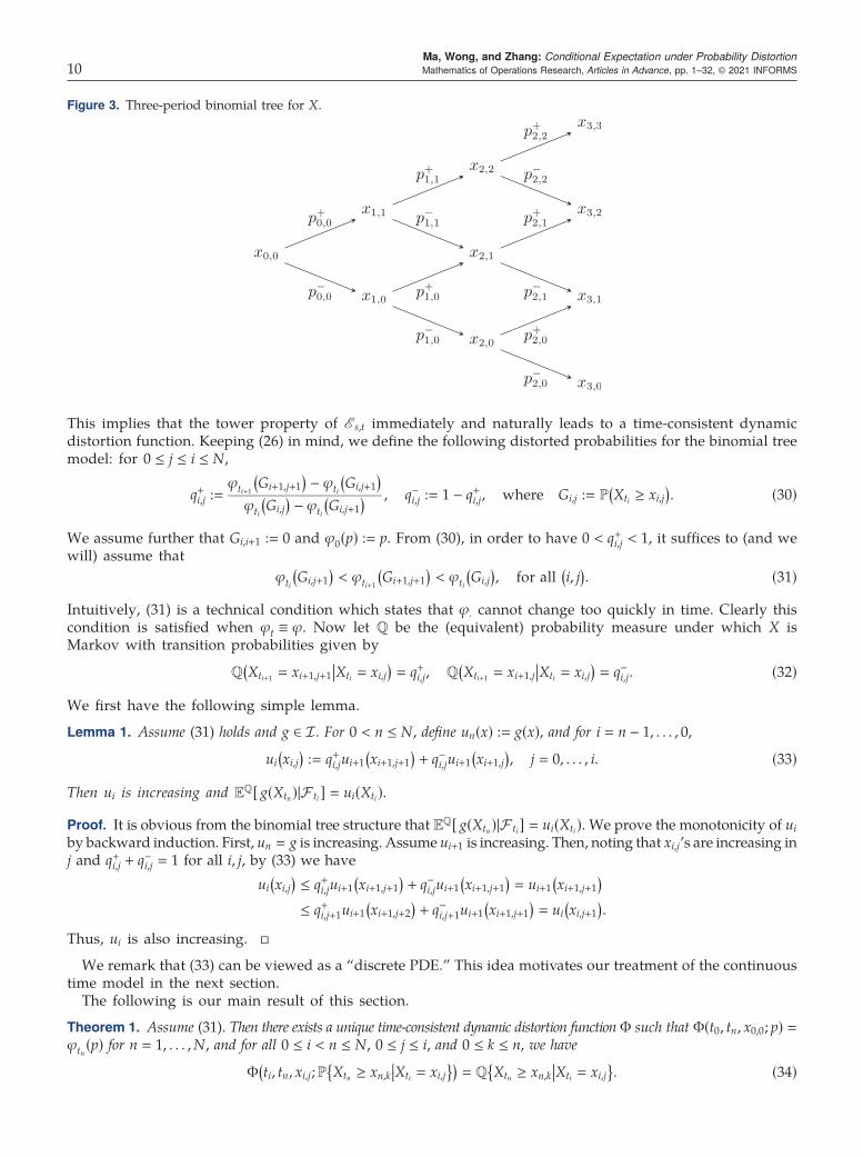
3.2. The General Binomial Tree CaseWe now extend our idea to a general binomial tree model. Let T consist of the points 0 � t0 < · · · < tN , and letX � {Xti}0≤i≤N be a finite-state Markov process such that, for each i � 0, . . . ,N, Xti takes values xi,0 < · · · < xi,iand has the following transition probabilities:

P Xti+1 � xi+1,j+1Xti � xi,j

( ) � p+i,j, P Xti+1 � xi+1,jXti � xi,j

( ) � p−i,j :� 1 − p+i,j, (28)where p±ij > 0 (see Figure 3 for the case N � 3). We also assume that for each ti ∈ T \ {0} we are given adistortion function ϕti .

Motivated by the analysis in Section 3.1, we shall find a distorted probability measure Q so that

E s,t g Xt( )[ ] � EQ g Xt( )|σ Xs( )[ ]for all g ∈ I . (29)


This implies that the tower property of E s,t immediately and naturally leads to a time-consistent dynamicdistortion function. Keeping (26) in mind, we define the following distorted probabilities for the binomial treemodel: for 0 ≤ j ≤ i ≤ N,

q+i,j :�ϕti+1 Gi+1,j+1

( ) − ϕti Gi,j+1( )

ϕti Gi,j( ) − ϕti Gi,j+1

( ) , q−i,j :� 1 − q+i,j, where Gi,j :� P Xti ≥ xi,j( )

. (30)

We assume further that Gi,i+1 :� 0 and ϕ0(p) :� p. From (30), in order to have 0 < q+i,j < 1, it suffices to (and wewill) assume that

ϕti Gi,j+1( )

< ϕti+1 Gi+1,j+1( )

< ϕti Gi,j( )

, for all i, j( )

. (31)Intuitively, (31) is a technical condition which states that ϕ· cannot change too quickly in time. Clearly thiscondition is satisfied when ϕt ≡ ϕ. Now let Q be the (equivalent) probability measure under which X isMarkov with transition probabilities given by

Q Xti+1 � xi+1,j+1Xti � xi,j

( ) � q+i,j, Q Xti+1 � xi+1,jXti � xi,j

( ) � q−i,j. (32)We first have the following simple lemma.

Lemma 1. Assume (31) holds and g ∈ I . For 0 < n ≤ N, define un(x) :� g(x), and for i � n − 1, . . . , 0,

ui xi,j( )

:� q+i,jui+1 xi+1,j+1( ) + q−i,jui+1 xi+1,j

( ), j � 0, . . . , i. (33)

Then ui is increasing and EQ[ g(Xtn)|F ti] � ui(Xti ).Proof. It is obvious from the binomial tree structure that EQ[ g(Xtn)|F ti] � ui(Xti). We prove the monotonicity of uiby backward induction. First, un � g is increasing. Assume ui+1 is increasing. Then, noting that xi,j’s are increasing inj and q+i,j + q−i,j � 1 for all i, j, by (33) we have

ui xi,j( ) ≤ q+i,jui+1 xi+1,j+1

( ) + q−i,jui+1 xi+1,j+1( ) � ui+1 xi+1,j+1

( )≤ q+i,j+1ui+1 xi+1,j+2

( ) + q−i,j+1ui+1 xi+1,j+1( ) � ui xi,j+1

( ).

Thus, ui is also increasing. □

We remark that (33) can be viewed as a “discrete PDE.” This idea motivates our treatment of the continuoustime model in the next section.

The following is our main result of this section.

Theorem 1. Assume (31). Then there exists a unique time-consistent dynamic distortion function Φ such that Φ(t0, tn, x0,0; p) �ϕtn(p) for n � 1, . . . ,N, and for all 0 ≤ i < n ≤ N, 0 ≤ j ≤ i, and 0 ≤ k ≤ n, we have

Φ ti, tn, xi,j;P Xtn ≥ xn,kXti � xi,j

{ }( ) � Q Xtn ≥ xn,kXti � xi,j

{ }. (34)

Figure 3. Three-period binomial tree for X.


Here uniqueness is only at the conditional survival probabilities for all k in the left-hand side of (34). Moreover, thecorresponding conditional nonlinear expectation satisfies (29).

Proof. We first show that (34) has a solution satisfying the desired initial conditon. Note that both P{Xtn ≥ xn,k |Xti �xi,j} and Q{Xtn ≥ xn,k |Xti � xi,j} are strictly decreasing in k, for fixed 0 ≤ i < n ≤ N and xi,j. Then one can easilydefine a function Φ, depending on ti, tn, xi,j, so that (34) holds for all xn,k, 0 ≤ k ≤ n. Moreover, the initial conditionΦ(t0, tn, x0,0; p) :� ϕtn(p) is equivalent to

ϕtn P Xtn ≥ xn,k{ }( ) � Q Xtn ≥ xn,k

{ }, 0 ≤ n ≤ N, 0 ≤ k ≤ n. (35)

We shall prove (35) by induction on n. First recall ϕ0(p) � p and that P{Xt0 � x0,0} � Q{Xt0 � x0,0} � 1; thus, (35)obviously holds for n � 0. Assume now it holds for n < N. Then

Q Xtn+1 � xn+1,k{ } � Q Xtn � xn,k−1

{ }q+n,k−1 +Q Xtn � xn,k

{ }q−n,k

� Q Xtn ≥ xn,k−1{ } −Q Xtn ≥ xn,k

{ }[ ]q+n,k−1 + Q Xtn ≥ xn,k

{ } −Q Xtn ≥ xn,k+1{ }[ ]

q−n,k� ϕtn Gn,k−1

( ) − ϕtn Gn,k( )[ ]

q+n,k−1 + ϕtn Gn,k( ) − ϕtn Gn,k+1

( )[ ]1 − q+n,k[ ]

� ϕtn+1 Gn+1,k( ) − ϕtn Gn,k

( )[ ]+ ϕtn Gn,k

( ) − ϕtn+1 Gn+1,k+1( )[ ]

� ϕtn+1 Gn+1,k( ) − ϕtn+1 Gn+1,k+1

( ).

This leads to (35) for n + 1 immediately and, thus, completes the induction step.We next show that the above-constructed Φ is indeed a time-consistent dynamic distortion function. We first

remark that, for this discrete model, only the values of Φ on the left-hand side of (34) are relevant, and one mayextendΦ to all p ∈ [0, 1] by linear interpolation. Then by (34) it is straightforward to show thatΦ(ti, tn, xi,j; ·) satisfiesDefinition 1(i). Moreover, by (16), (8), and (34), for any g ∈ I we have

E ti ,tn g Xtn( )[ ]

Xti�xi,j �∑nk�0

g xn,k( )

Φ ti, tn, xi,j;P Xtn ≥ xn,kXti � xi,j

{ }( )[−Φ ti, tn, xi,j;P Xtn ≥ xn,k+1

Xti � xi,j

{ }( )]� ∑n

k�0g xn,k( )

Q Xtn ≥ xn,kXti � xi,j

{ } −Q Xtn ≥ xn,k+1Xti � xi,j

{ }[ ]� EQ g Xtn

( )Xti � xi,j

[ ].

That is, (29) holds. Moreover, fix n and g, and let ui be as in Lemma 1. Since um is increasing, we have

E ti,tm E tm ,tn g Xtn( )[ ][ ] � E ti,tm um Xtm

( )[ ] � ui Xti( ) � E ti,tn g Xtn

( )[ ], 0 ≤ i < m < n.

This verifies (17). Thus, Φ is a time-consistent dynamic distortion function.It remains to prove the uniqueness of Φ. Assume Φ is an arbitrary time-consistent dynamic distortion function.

For any appropriate i, j, and g ∈ I , following the arguments of Lemma 1 we see that

u ti, xi,j( )

:� E ti,ti+1 g Xti+1( )[ ]

Xti�xi,j

� g xi+1,j( )

1 − Φ ti, ti+1, xi,j; p+i,j( )[ ]

+ g xi+1,j+1( )

Φ ti, ti+1, xi,j; p+i,j( )

is increasing in xi,j. Then by (8) and the tower property we have∑kg xi+1,k( )

ϕti+1 Gi+1,k( ) − ϕti+1 Gi+1,k+1

( )[ ]� E 0,ti+1 g Xti+1

( )[ ] � E 0,ti E ti,ti+1 g Xti+1( )[ ][ ]

.

� E 0,ti u ti,Xti( )[ ] � ∑

ju ti, xi,j( )

ϕti Gi,j( ) − ϕti Gi,j+1

( )[ ]� ∑

jg xi+1,j( )

1 −Φ ti, ti+1, xi,j; p+i,j( )[ ]

+ g xi+1,j+1( )

Φ ti, ti+1, xi,j; p+i,j( )[ ]

× ϕti Gi,j( ) − ϕti Gi,j+1

( )[ ].


By the arbitrariness of g ∈ I , this implies that

1 − ϕti+1 Gi+1,1( ) � 1 − Φ ti, ti+1, xi,0; p+i,0( )[ ]

1 − ϕti Gi,1( )[ ]

;

ϕti+1 Gi+1,k( ) − ϕsti+1 Gi+1,k+1

( ) � 1 −Φ ti, ti+1, xi,k; p+i,k( )[ ]

ϕti Gi,k( ) − ϕti Gi,k+1

( )[ ]+Φ ti, ti+1, xi,k−1; p+i,k−1

( )ϕti Gi,k−1

( ) − ϕti Gi,k( )[ ]

, k � 1, . . . , i + 1.

This is equivalent to, denoting ak :� Φ(ti, ti+1, xi,k; p+i,k)[ϕti (Gi,k) − ϕti (Gi,k+1)],a0 � ϕti+1 Gi+1,1( ) − ϕti Gi,1( );

ak−1 − ak � ϕti+1 Gi+1,k( ) − ϕti+1 Gi+1,k+1

( )[ ]− ϕti Gi,k

( ) − ϕti Gi,k+1( )[ ]

.

Clearly the above equations have a unique solution, so we must have Φ(ti, ti+1, xi,k; p+i,k) � q+i,k. This impliesfurther that E ti ,ti+1[g(Xti+1 )] � EQ[g(Xti+1 )|F ti .]. Now both E ti,tn and EQ[·|·] satisfy the tower property. ThenE ti ,tn[g(Xtn)] � EQ[g(Xtn)|F ti .] for all ti < tn and all g ∈ I . So E ti ,tn is unique, which implies immediately theuniqueness of Φ. □

Remark 5.(i) We should note that the dynamic distortion function Φ that we constructed actually depends on the

survival function of X under both P and Q (see also (57)).(ii) Our construction of Φ is local in time. In particular, all the results can be easily extended to the case with

infinite times: 0 � t0 < t1 < · · ·.(iii) Our construction of Φ is also local in state, in the sense that Φ(ti, tn, xi,j; ·) involves only the subtree

rooted at (ti, xi,j).

4. The Constant-Diffusion CaseIn this section we set T � [0,T] and consider the case where the underlying state process X is a one-dimensional Markov process satisfying the following SDE with constant-diffusion coefficient:

Xt � x0 +∫ t

0b s,Xs( )ds + Bt, (36)

where B is a one-dimensional standard Brownian motion on a given filtered probability space (Ω,F , {F t}0≤t≤T,P).Again we are given initial distortion functions {ϕt � ϕ(t, ·)}0<t≤T and ϕ0(p) ≡ p. Our goal is to construct a time-consistent dynamic distortion function Φ and the corresponding time-consistent distorted conditional ex-pectations E s,t for (s, t) ∈ T 2. We shall impose the following technical conditions.

Assumption 1. The function b is sufficiently smooth, and both b and the required derivatives are bounded.

Clearly, under the assumption the SDE (36) is well posed. The further regularity of b is used to derive sometail estimates for the density of Xt, which are required for our construction of the time-consistent dynamicdistortion function Φ and the distorted probability measure Q. By investigating our arguments more carefully,we can figure out the precise technical conditions we will need. However, since our main focus is the dynamicdistortion function Φ, we prefer not to carry out these details for the sake of the readability of the paper.

4.1. Binomial Tree ApproximationOur idea is to approximate X by a sequence of binomial trees and then apply the results from the previoussection. To this end, for fixed N, denote h :� T/N and ti :� ih, i � 0, · · · ,N. Then (36) may be discretizedas follows:

Xti+1 ≈ Xti + b ti,Xti( )

h + Bti+1 − Bti . (37)We first construct the binomial tree on T N :� {ti, i � 0, . . . ,N} as in Section 3.2 with

x0,0 � x0, xi,j � x0 + 2j − i( )

h√

, bi,j :� b ti, xi,j( )

, p+i,j :�12+ 12bi,j

h

√. (38)


Since b is bounded, we shall assume h is small enough so that 0 < p+i,j < 1. Let XN denote the Markov chaincorresponding to this binomial tree under the probability PN specified by (38). Then our choice of p+i,j en-sures that

EPN XNti+1 − XN

ti

XN

ti � xi,j[ ]

� p+i,jh

√ − p−i,jh

√ � bi,jh;

EPN XNti+1 − XN

ti − bi,jh( )2

XNti � xi,j

[ ]� p+i,j

h

√ − bi,jh( )2 + p−i,j

h

√ + bi,jh( )2� h − b2i,jh

2.(39)

Clearly, as a standard Euler approximation, XN matches the conditional expectation and conditional varianceof X in (37), up to terms of order o(h).

Next we define the other terms in Section 3.2:

GNi,j :� PN XN

ti ≥ xi,j{ )

, qN,+i,j :�

ϕti+1 GNi+1,j+1

( )−ϕti

GNi,j+1

( )ϕti

GNi,j

( )−ϕti

GNi,j+1

( ) , qN,−i,j :� 1 − qN,+

i,j ;

QN XNti+1 � xi+1,j+1

XN

ti � xi,j{ }

� qN,+i,j , QN XN

ti+1 � xi+1,jXN

ti � xi,j{ }

� qN,−i,j ;

ΦN ti, tn, xi,j;PN XNtn ≥ xn,k

XN

ti � xi,j{ }( )

:� QN XNtn ≥ xn,k

XN

ti � xi,j{ }

.

⎧⎪⎪⎪⎪⎪⎪⎪⎪⎪⎪⎪⎪⎪⎪⎪⎪⎪⎪⎪⎪⎪⎨⎪⎪⎪⎪⎪⎪⎪⎪⎪⎪⎪⎪⎪⎪⎪⎪⎪⎪⎪⎪⎪⎩(40)

We shall send N → ∞ and analyze the limits of the above terms. In this section we evaluate the limitsheuristically, by assuming all functions involved exist and are smooth.

Define the survival probability function and density function of the X in (36), respectively:

G t, x( ) :� P Xt ≥ x( ), ρ t, x( ) :� −∂xG t, x( ), 0 < t ≤ T. (41)Note that, as the survival function of the diffusion process (36), G satisfies the following PDE:

∂tG � 12∂xxG − b∂xG � − 1

2∂xρ + bρ. (42)

It is reasonable to assume GNi,j ≈ G(ti, xi,j). Note that ti+1 � ti + h, xi,j+1 � xi,j + 2

h

√, xi+1,j+1 � xi,j +

h

√. Rewrite

ϕ(t, p) :� ϕt(p). Then, for (t, x) � (ti, xi,j), by (42) and applying Taylor expansion we have (suppressing variableswhen the context is clear):

ϕ t + h,G t + h, x + h

√( )( )− ϕ t,G t, x( )( )

� ∂tϕh + ∂pϕ ∂tGh + ∂xGh

√ + 12∂xxGh

[ ]+ 12∂ppϕ ∂xG[ ]2h + o h( )

� −∂pϕρh

√ + ∂tϕ + ∂pϕbρ − ∂pϕ∂xρ + 12∂ppϕρ

2[ ]

h + o h( );

ϕ t,G t, x + 2h

√( )( )− ϕ t,G t, x( )( ) � ∂pϕ ∂xG2

h

√ + 12∂xxG4h

[ ]+ 12∂pp ∂xG[ ]24h + o h( )

� −2∂pϕρh

√ − 2 ∂pϕ∂xρ − ∂ppϕρ2[ ]h + o h( ).

Thus, we have an approximation for the qN,+i,j in (40):

qN,+i,j ≈

ϕ t + h,G t + h, x + h

√( )( )− ϕ t,G t, x + 2

h

√( )( ).

ϕ t,G t, x( )( ) − ϕ t,G t, x + 2h

√( )( )� 1 + −∂pϕρ

h

√ + ∂tϕ + ∂pϕbρ − ∂pϕ∂xρ + 12 ∂ppϕρ

2[ ]

h + o h( )2∂pϕρ

h

√ + 2 ∂pϕ∂xρ − ∂ppϕρ2[ ]

h + o h( )� 12+ 12μ t, x( )

h

√ + oh

√( ), (43)


where

μ t, x( ) :� b t, x( ) + ∂tϕ t,G t, x( )( ) − 12 ∂ppϕ t,G t, x( )( )ρ2 t, x( )

∂pϕ t,G t, x( )( )ρ t, x( ) . (44)

Next, note that

EQN XNti+1 − XN

ti

XN

ti � xi,j{ }

� h

√2qN,+

i,j − 1[ ]

� μ ti, xi,j( )

h + o h( );

EQN XNti+1 − XN

ti − μ ti, xi,j( )

h( )2

XNti � xi,j

{ }� h + o h( ).

In other words, as N → ∞, we expect that QN would converge to a probability measure Q such that, for someQ-Brownian motion B, it holds that

Xt � x0 +∫ t

0μ s,Xs( )ds + Bt, Q-a.s. (45)

Moreover, formally one should be able to find a dynamic distortion function Φ satisfying:

Φ s, t, x;P Xt ≥ y|Xs � x{ }( ) � Q Xt ≥ y|Xs � x

{ }, 0 ≤ s < t ≤ T. (46)

We shall note that, however, since X0 � x0 is degenerate, ρ(0, ·) and hence μ(0, ·) do not exist, so the aboveconvergence will hold only for 0 < s < t ≤ T. It is also worth noting that asymptotically (33) should read:

u t, x( ) ≈ 12

1 + μ t, x( )h

√ + oh

√( )[ ]u t + h, x +

h√( )

− u t + h, x − h

√( )[ ]+ u t + h, x −

h√( )

� u t, x( ) + ∂tu + 12∂xxu + μ∂xu

[ ]h + o h( ).

That is,

L u t, x( ) :� ∂tu + 12∂xxu + μ∂xu � 0. (47)

4.2. Rigorous Results for the Continuous Time ModelWe now substantiate the heuristic arguments in the previous section and derive the time-consistent dynamicdistortion function and the distorted conditional expectation for the continuous time model. We first have thefollowing tail estimates for the density of the diffusion (36). Since our main focus is the dynamic distortionfunction, we postpone the proof to Section 6.

Proposition 3. Under Assumption 1, Xt has a density function ρ(t, x) which is strictly positive and sufficiently smooth on(0,T] × R. Moreover, for any 0 < t0 ≤ T, there exists a constant C0, possibly depending on t0, such that

|∂xρ t, x( )|ρ t, x( ) ≤ C0,

1C0 1 + |x|[ ] ≤

G t, x( ) 1 − G t, x( )[ ]ρ t, x( ) ≤ C0, t, x( ) ∈ t0,T[ ] × R. (48)

We next assume the following technical conditions on ϕ.

Assumption 2. ϕ is continuous on [0,T] × [0, 1] and is sufficiently smooth in (0,T] × (0, 1) with ∂pϕ > 0. Moreover, forany 0 < t0 < T, there exists a constant C0 > 0 such that for (t, p) ∈ [t0,T] × (0, 1) we have the following bounds:

∂ppϕ t, p( )

∂pϕ t, p( )

≤ C0

p 1 − p( ) , ∂pppϕ t, p

( )∂pϕ t, p

( )

≤ C0

p2 1 − p( )2 , (49)

∂tϕ t, p( )

∂pϕ t, p( )

≤ C0p 1 − p

( ),

∂tpϕ t, p( )

∂pϕ t, p( )

≤ C0. (50)

We note that, given the existence of G(t, x) and ρ(t, x) as well as the regularity of ϕ, the function μ(t, x) in (44) iswell defined.


Remark 6.(i) Note that in (43) and (44) only the composition ϕ(t,G(t, x)) is used, and obviously 0 < G(t, x) < 1 for all

(t, x) ∈ (0,T] × R. Therefore, we do not require the differentiability of ϕ at p � 0, 1. Moreover, since ∂pϕ > 0, thecondition (49) involves only the singularities around p ≈ 0 and p ≈ 1.

(ii) The first line in (49) is not restrictive. For example, by straightforward calculation one can verify that allthe following distortion functions commonly used in the literature (see, e.g., Huang et al. [12, section 4.2])satisfy it: recalling that in the literature typically ϕ(t, p) � ϕ(p) does not depend on t.

• Tversky and Kahneman [23]: ϕ(p) � pγ/[pγ + (1 − p)γ]1/γ, γ ∈ [γ0, 1), where γ0 ≈ 0.279 so that ϕis increasing.

• Tversky and Fox [22]: ϕ(p) � αpγ/[αpγ + (1 − p)γ], α > 0, γ ∈ (0, 1).• Prelec [20]: ϕ(p) � exp(−γ(− ln p)α), γ > 0, α ∈ (0, 1).• Wang [24]: ϕ(p) � F(F−1(p) + α), α ∈ R, where F is the cdf of the standard normal.

As an example, we check the last one, which is less trivial. Set q :� F−1(p). Then

ϕ F q( )( ) � F q + α

( )�⇒ϕ′ F q( )( ) � F′ q + α

( )F′ q

( ) �⇒ ln ϕ′ F q( )( )( ) � ln F′ q + α

( )( ) − ln F′ q( )( )

.

Note that F′(q) � e−q2/2/2π

√. Then ln(F′(q)) � − ln

2π

√ − q/2. Thus,

ln ϕ′ F q( )( )( ) � − q + α

( )22

+ q2

2�⇒ ϕ′′ F q

( )( )ϕ′ F q

( )( ) F′ q( ) � −α.

This implies that, denoting by G(q) :� 1 − F(q) the survival function of the standard normal,

|ϕ′′ p( )|

ϕ′ p( ) p 1 − p

[ ] � |α| F q( )

1 − F q( )[ ]

F′ q( ) � |α|G q

( )1 − G q

( )[ ]F′ q

( ) .

Then by applying (48) on the standard normal (namely, b � 0 and t � 1 there) we obtain the desired estimatefor ∂ppϕ

∂pϕ. Similarly we may estimate ∂pppϕ

∂pϕ.

(iii) When ϕ(t, p) ≡ ϕ(p) as in the standard literature, the second line in (49) is trivial. Another importantexample is the separable case: ϕ(t, p) � f (t)ϕ0(p). Assume f ′ is bounded. Then the second inequality herebecomes trivial, and a sufficient condition for the first inequality is ϕ0(p)

ϕ′0(p) ≤

C0p(1−p), which holds true for all the

examples in (ii).

To have a better understanding about μ given by (44), we compute an example explicitly.

Example 4. Consider Wang’s [24] distortion function: ϕ(t, p) � F(F−1(p) + α), as in Remark 6(ii). Set b � 0.Then μ(t, x) � α/2 t

√.

Proof. First it is clear that ∂tϕ � 0 and ∂pϕ(t, p) � F′(F−1(p) + α)/F′(F−1(p)). Then∂ppϕ t, p

( )∂pϕ t, p

( ) � ∂p ln ∂pϕ t, p( )( )[ ] � 1

F′ F−1 p( )( ) F′′ F−1 p

( ) + α( ))

F′ F−1 p( ) + α

( )) − F′′ F−1 p( )( )

F′ F−1 p( )( )[ ]

.

One can easily check that F′(x) � e−x2/2/2π

√and F′′(x) � −xF′(x). Then

∂ppϕ t, p( )

∂pϕ t, p( ) � 1

F′ F−1 p( )( ) − F−1 p

( ) + α[ ] + F−1 p

( )[ ] � − α

F′ F−1 p( )( ) .

Note that

G t, x( ) � P Bt ≥ x( ) � P B1 ≥ x

t√

( )� P B1 ≤ − x

t√

( )� F − x

t√

( ).

Then

μ t, x( ) � αρ t, x( )F′ F−1 G t, x( )( )( ) �

αρ t, x( )F′ −x/ t

√( ) �α 2πt

√ e−x22t

12π

√ e−−x/ t

√( )22

� α

t√ ,


completing the proof.

We now give some technical preparations. Throughout the paper we shall use C to denote a generic constantwhich may vary from line to line.

Lemma 2. Let Assumptions 1 and 2 hold.(i) The function μ defined by (44) is sufficiently smooth in (0,T] × R. Moreover, for any 0 < t0 < T, there exists

C0 > 0 such that

|μ t, x( )| ≤ C0 1 + |x|[ ], |∂xμ t, x( )| ≤ C0 1 + |x|2[ ], for all t, x( ) ∈ t0,T[ ] × R. (51)

(ii) For any (s, x) ∈ (0,T) × R, the following SDE on [s,T] has a unique strong solution:

Xs,xt � x +

∫ t

sμ r, Xs,x

r

( )dr + Bs

t , where Bst :� Bt − Bs, t ∈ s,T[ ], P-a.s.. (52)

Moreover, the following Ms,x is a true P-martingale and P ◦ (Xs,x)−1 � Qs,x ◦ (Xs,x)−1, where

Xs,xt :� x + Bs

t , Ms,xt :� e

∫ t

sμ r,Xs,x

r( )dBr−12

∫ t

s|μ r,Xs,x

r( )|2dr,dQs,x

dP:� Ms,x

T . (53)

(iii) Recall the process X as in (36). Define

Gs,xt y

( ):� P Xt ≥ y|Xs � x

( ), Gs,x

t y( )

:� P Xs,xt ≥ y

( ), 0 < s < t ≤ T, x, y ∈ R. (54)

Then Gs,xt and Gs,x

t are continuous, strictly decreasing in y, and enjoy the following properties:

Gs,xt ∞( ) :� lim

y→∞Gs,xt y

( ) � 0, Gs,xt ∞( ) :� lim

y→∞ Gs,xt y

( ) � 0;

Gs,xt −∞( ) :� lim

y→−∞Gs,xt y

( ) � 1, Gs,xt −∞( ) :� lim

y→−∞ Gs,xt y

( ) � 1.

Furthermore, Gs,xt has a continuous inverse function (Gs,x

t )−1 on (0, 1), and by continuity we set (Gs,xt )−1

(0) :� −∞, (Gs,xt )−1(1) :� ∞.

(iv) For any g ∈ I fixed, let u(t, x) :� EP[g(Xt,xT )], (t, x) ∈ (0,T] × R. Then u is bounded, is increasing in x, and is the

unique bounded viscosity solution of the following PDE:

L u t, x( ) :� ∂tu + 12∂xxu + μ∂xu � 0, 0 < t ≤ T; u T, x( ) � g x( ). (55)

(v) For the t0 and C0 in (i), there exists δ � δ(C0) > 0 such that if g ∈ I is sufficiently smooth and g′ has compactsupport, then u is sufficiently smooth on [T − δ,T] × R and there exists a constant C > 0, which may depend on g,satisfying, for (t, x) ∈ [T − δ,T] × R,

u t, x( ) − g −∞( ) ≤ Ce−x2, x < 0; |u t, x( ) − g ∞( )| ≤ Ce−x

2, x > 0; ∂xu t, x( ) ≤ Ce−x

2. (56)

Proof. (i) By our assumptions and Proposition 3, the regularity of μ follows immediately. For any t ≥ t0, by (49) andthen (48) we have

∂tϕ t,G t, x( )( )∂pϕ t,G t, x( )( )ρ t, x( )

≤ CG t, x( ) 1 − G t, x( )[ ]

ρ t, x( ) ≤ C;

∂ppϕ t,G t, x( )( )ρ t, x( )∂pϕ t,G t, x( )( )

≤ Cρ t, x( )

G t, x( ) 1 − G t, x( )[ ] ≤ C 1 + |x|[ ].

Then it follows from (44) that |μ(t, x)| ≤ C[1 + |x|].Moreover, note that

∂xμ t, x( ) � ∂xb − ∂tpϕ

∂pϕ+ ∂tϕ∂ppϕ

∂pϕ( )2 − ∂tϕ∂xρ

∂pϕρ2 + 12∂pppϕρ2

∂pϕ− 12∂ppϕ∂xρ

∂pϕ− 12

∂ppϕ( )2ρ2

∂pϕ( )2 .


By (49) and (48) again one can easily verify that |∂xμ(t, x)| ≤ C0[1 + |x|2].(ii) Since μ is locally uniform Lipschitz continuous in x, by a truncation argument Xs,x exists locally. Now

the uniform linear growth (51) guarantees the global existence. Moreover, by [14, chapter 3, corollary 5.16] we seethat Mt,x is a true P-martingale and thus Qt,x is a probability measure.

(iii) Since the conditional law of Xt under P given Xs � x has a strictly positive density, the statementsconcerning Gs,x

t are obvious. Similarly, since the law of Xs,xt under P has a density and dQs,x � dP, the

statements concerning Gs,xt are also obvious.

(v) We shall prove (v) before (iv). Let δ > 0 be specified later, and let t ∈ [T − δ,T]. Let R > 0 be such thatg′(x) � 0 for |x| ≥ R. Note that u(t, x) � E[Mt,x

T g(Xt,xT )]. For x > 2R, we have

u t, x( ) − g ∞( ) � E Mt,xT g Xt,x

T

( ) − g ∞( )[ ][ ] ≤ E Mt,xT |g Xt,x

T

( ) − g ∞( )|[ ]≤ 2‖g‖∞E Mt,x

T 1 Xt,xT ≤R{ }

[ ]� 2‖g‖∞E e

∫ T

tμdBr−3

2

∫ T

t|μ|2dre

∫ T

t|μ|2dr1 Xt,x

T ≤R{ }[ ]

.

Then

u t, x( ) − g ∞( ) 3≤ ‖g‖3∞E e3∫ T

tμdBr−9

2

∫ T

t|μ|2dr[ ]

E e3∫ T

t|μ|2dr[ ]

P Xt,xT ≤ R

( ).

By [14, chapter 3, corollary 5.16] again, we have E[e3∫ T

tμdBr−9

2

∫ T

t|μ|2dr] � 1. By (51), we have

E e3∫ T

t|μ|2dr[ ]

≤ E eC0∫ T

t1+|x|2+|Bt

r |2[ ]dr[ ]≤ eC0δ 1+|x|2[ ]E e

C0δ sup0≤s≤δ

|Bs |2[ ]≤ e2C0δ 1+|x|2[ ],

for δ small enough. Fix such a δ > 0, and let t ∈ [T − δ,T]. Note that we may choose δ independent from g.Henceforth, we let C > 0 be a generic constant. Moreover, since x > 2R,

P Xt,xT ≤ R

( ) ≤ P Xt,xT ≤ x

2

( )� P Bt

T ≤ − x2

( )≤ P B1 ≤ − x

2δ

√( )

≤ Ce−x28δ.

Putting these statements together, we have, for δ small enough,

u t, x( ) − g ∞( ) 3≤ Ce−x28δ+Cδ 1+|x|2[ ] ≤ Ce−3x

2.

This implies that |u(t, x) − g(∞)| ≤ Ce−x2 . Similarly, |u(t, x) − g(−∞)| ≤ Ce−x2 for x < 0.The preceding estimates allows us to differentiate inside the expectation, and we have

∂xu t, x( ) � E g′ Xt,xT

( )∇Xt,xT

[ ],

where ∇Xt,xs � 1 +

∫ s

t∂xμ r, Xt,x

r

( )∇Xt,xr dr and thus ∇Xt,x

T � e∫ T

t∂xμ s,Xt,x

s( )ds > 0.

Then ∂xu ≥ 0. Moreover, recalling (53) we have

∂xu t, x( ) � E g′ Xt,xT

( )e∫ T

t∂xμ s,Xt,x

s( )ds[ ]� E Mt,x

T g′ Xt,xT

( )e∫ T

t∂xμ s,Xt,x

s( )ds[ ]≤ CE Mt,x

T e∫ T

t∂xμ s,Xt,x

s( )ds1 |Xt,xT |≤R{ }

[ ].

Then, by the estimate of ∂xμ in (51), it follows from the same arguments as above that we can showthat |∂xu(t, x)| ≤ Ce−x2 .

Finally, we may apply the arguments further to show that u is sufficiently smooth, and then it follows from the flowproperty and the standard Itô formula that u satisfies PDE (55).

(iv) We shall only prove the results on [T − δ,T]. Since δ > 0 depends only on C0 in (i), one may apply theresults backwardly in time and extend the results to [t0,T]. Then it follows from the arbitrariness of t0 that theresults hold true on (0,T].

We now fix δ as in (v). The boundedness of u is obvious. Note that u(t, x) � EP[g(Xt,xT )Mt,x

T ], and μ and g are continuous.Following similar arguments as in (v) one can show that u is continuous.

Next, for any g ∈ I , there exist approximating sequences {gn} such that each gn satisfies the conditions in (v). Letun(t, x) :� E[ gn(Xt,x

T )]. Then un is increasing in x and is a classical solution to PDE (55) on [T − δ,T]with terminal condition gn.It is clear that un → u. Then u is also increasing in x, and its viscosity property follows from the stability of viscosity solutions.


The uniqueness of the viscosity solution follows from the standard comparison principle. We refer to the classical referenceCrandall et al.[5] for the details of the viscosity theory. □

We are now ready for the main result of this section. Recall (54), and define

Φ s, t, x; p( )

:� Gs,xt Gs,x

t

( )−1 p( )( )

, s > 0. (57)

Theorem2. LetAssumptions 1 and 2 hold. ThenΦ defined by (57) is a time-consistent dynamic distortion function which isconsistent with the initial conditions: Φ(0, t, x; p) � ϕt(p).Proof. First, by Lemma 2(iv) it is straightforward to check that Φ satisfies Definition 2(i).

Next, for 0 < s < t ≤ T, note that the definition (57) of Φ implies the counterpart of (34):

Φ s, t, x;Gs,xt y

( )( ) � Gs,xt y

( ). (58)

Recall (16) and Lemma 2. One can easily see that E s,t[g(Xt)] � u(s,Xs) for any g ∈ I , where u(s, x) :� EP[g(Xs,xt )]

is increasing in x and is the unique viscosity solution of the PDE (55) on [s, t] × R with terminal conditionu(t, x) � g(x). Then, either by the flow property of the solution to SDE (52) or the uniqueness of the PDE, weobtain the tower property (17) immediately for 0 < r < s < t ≤ T.

To verify the tower property at r � 0, let t0 > 0 and δ > 0 be as in Lemma 2(v). We first show that, for any g as inLemma 2(v) and the corresponding u, we have

E 0,t1 u t1,Xt1( )[ ] � E 0,t2 u t2,Xt2

( )[ ], T − δ ≤ t1 < t2 ≤ T. (59)

Clearly the set of such g is dense in I . Then (59) holds true for all g ∈ I , where u is the viscosity solution to thePDE (55). Note that u(t,Xt) � E t,T[ g(XT)]. Then by setting t1 � t and t2 � T in (59) we obtain E 0,t[E t,T[g(XT)]] �E 0,T[ g(XT)] for T − δ ≤ t ≤ T. Similarly we can verify the tower property over any interval [t − δ, t] ⊂ [t0,T].Since Es,t is already time consistent for 0 < s < t, we see the time consistency for any t0 ≤ s < t ≤ T. Now by thearbitrariness of t0 > 0, we obtain the tower property at r � 0 for all 0 < s < t ≤ T.

We now prove (59). Recall from (56) that u(t,−∞) � g(−∞) � 0. Then, for T − δ ≤ t ≤ T, similar to (10), we have

E 0,t u t,Xt( )[ ] �∫ ∞

0ϕ t,P u t,Xt( ) ≥ x( )( )dx �

∫R

ϕ t,G t, x( )( )∂xu t, x( )dx.

Let ψm : R → [0, 1] be smooth with ψm(x) � 1, |x| ≤ m, and ψm(x) � 0, |x| ≥ m + 1. Denote

E m0,t u t,Xt( )[ ] :�

∫R

ϕ t,G t, x( )( )∂xu t, x( )ψm x( )dx.Then, recalling (42) and (55) and suppressing the variables when the context is clear, we have

ddt

E m0,t u t,Xt( )[ ] �

∫R

∂tϕ + ∂pϕ∂tG[ ]

∂xu + ϕ∂txu[ ]

ψmdx

�∫R


∂xuψm + ∂pϕρψm − ϕψ′m

[ ]∂tu

[ ]dx

�∫R

∂tϕ + ∂pϕ bρ − 12∂xρ

[ ][ ]ψm∂xu − ∂pϕρψm − ϕψ′

m

[ ] 12∂xxu + μ∂xu

[ ][ ]dx

�∫R


[ ]− ∂pϕρμ

[ ]ψm∂xu + ϕψ′

mμ∂xu[

+ 12∂xu ∂pϕ∂xρψm − ∂ppϕρ

2ψm + 2∂pϕρψ′m − ϕψ′′

m

[ ]]dx

�∫R

∂tϕ + ∂pϕbρ − ∂pϕρμ − 12∂ppϕρ

2[ ]

ψm + ϕμ + ∂pϕρ[ ]

ψ′m − 1

2ϕψ′′

m

[ ]∂xudx

�∫R

ϕμ + ∂pϕρ[ ]

ψ′m − 1

2ϕψ′′

m

[ ]∂xudx, (60)


where the last equality follows from (44). That is, for any T − δ ≤ t1 < t2 ≤ T,

E m0,t2 u t2,Xt2

( )[ ] − E m0,t1 u t1,Xt1

( )[ ] � ∫ t2

t1

∫R

ϕμ + ∂pϕρ[ ]

ψ′m − 1

2ϕψ′′

m

[ ]∂xudxdt. (61)

It is clear that limm→∞ E m0,t[u(t,Xt)] � E 0,t[u(t,Xt)]. Note that, by (51) and (56), we have

|μ| ≤ C 1 + |x|[ ], ∂pϕρ ≤ CρG 1 − G[ ] ≤ C 1 + |x|[ ], |∂xu| ≤ Ce−x

2.

Then, by sending m → ∞ in (61) and applying the dominated convergence theorem, we obtain (59) and hencethe theorem. □

Remark 7. In the definition ofΦ (see (57)) we require that the initial time s is strictly positive. In fact, when s � 0 thedistribution of Xs becomes degenerate, and thus, μ may have singularities. For example, assume ϕ(t, ·) � ϕ(·) isindependent of t and b ≡ 0, x0 � 0. Then

μ t, x( ) � − ϕ′′ G t, x( )( )2ϕ′ G t, x( )( )

12

πt

√ e−x22t .

It is not even clear if the following SDE is well posed in general:

Xt �∫ t

0μ s, Xs( )

ds + Bt.

Correspondingly, if we consider the following PDE on (0,T] × R:

L u t, x( ) � 0, t, x( ) ∈ 0,T( ] × R, u T, x( ) � g x( ),then it is not clear whether lim(t,x)→(0,0) u(t, x) exists.

Unlike Theorem 1 in the discrete case, surprisingly here the time-consistent dynamic distortion function isnot unique. Let Φ be an arbitrary time-consistent dynamic distortion function for 0 < s < t ≤ T (not necessarilyconsistent with ϕt when s � 0 at this point). Fix 0 < t ≤ T. For any s ∈ (0, t] and g ∈ I , define

u s, x( ) :�∫R

Φ s, t, x;P g Xt( ) ≥ y|Xs � x( )( )

ds. (62)

The corresponding {E s,t} is time consistent, that is, the tower property holds. Suppose Φ defines via (58) aQ-diffusion X with coefficients μ, σ, that is,

Φ s, t, x;P Xt ≥ y|Xs � x( )( ) � P Xs,x

t ≥ y( )

,where Xs,xt � x +

∫ t

sμ r, Xs,x

r

( )dBr +

∫ t

sσ r, Xs,x

r

( )dBr, P-a.s., (63)

and u satisfies the following PDE corresponding to the infinitesimal generator of X:

∂tu + 12σ2∂xxu + μ∂xu � 0, s, x( ) ∈ 0, t( ] × R; u t, x( ) � g x( ). (64)

We have the following more general result.

Theorem 3. Let Assumptions 1 and 2 hold, and let Φ be an arbitrary smooth time-consistent (for t > 0) dynamic distortionfunction corresponding to (63). Suppose μ and σ are sufficiently smooth such that u is smooth and integration by parts in (66)below goes through. Then Φ is consistent with the initial condition Φ(0, t, x; p) � ϕt(p) if and only if

μ � b + σ∂xσ + 12

σ2 − 1[ ] ∂xρ

ρ+ ∂tϕ

∂pϕρ− σ2∂ppϕρ

2∂pϕ. (65)

In particular, if we restrict to the case σ � 1, then μ � μ and hence Φ � Φ is unique.


Proof. The consistency of Φ with the initial condition Φ(0, t, x; p) � ϕt(p) is equivalent to (59) for u, where u is thesolution to PDE (64) on (0,T] with terminal condition g. Similar to (60), we have

ddtE 0,t u t,Xt( )[ ] �

∫R


∂xu + ϕ∂txu[ ]

dx

�∫R


∂xu + ∂pϕρ∂tu[ ]

dx

�∫R


[ ][ ]∂xu − ∂pϕρ

12σ2∂xxu + μ∂xu

[ ][ ]dx

�∫R


[ ]− ∂pϕρμ

[ ]∂xu

[+ 12∂xu −∂ppϕρ2σ2 + ∂pϕ∂xρσ

2 + 2∂pϕρσ∂xσ[ ]]

dx

�∫R

b + σ∂xσ + ∂tϕ

∂pϕρ− σ2∂ppϕρ

2∂pϕ+ 12

σ2 − 1[ ] ∂xρ

ρ

[− μ

]∂pϕρ∂xudx. (66)

Since ∂pϕρ > 0 and since g (and hence u) is arbitrary, we get the equivalence of (59) and (65). □

Remark 8.(i) When σ �≡ 1, the law of Xs,x

t can be singular to the conditional law of Xt given Xs � x. That is, the agentmay distort the probability so dramatically that the distorted probability is singular to the original one. Forexample, some event which is null under the original probability may be distorted into a positive or even fullmeasure, so the agent could be worrying too much on something which could never happen, which does notseem to be reasonable in practice. Our result says that if we exclude this type of extreme distortion, then forgiven {ϕt}, the time-consistent dynamic distortion function Φ is unique.

(ii) In the discrete case in Section 3.2, because of the special structure of the binomial tree, we always have|Xti+1 − Xti |2 � h. Then for any possible Q, we always have EQ[|Xti+1 − Xti |2|Xti � xi,j] � h. This, in the continuoustime model, means σ ≡ 1. This is why we can obtain the uniqueness in Theorem 1.

4.3. Rigorous Proof of the ConvergenceWe note that Theorem 2 already gives the definition of the desired time-consistent conditional expectation forthe constant-diffusion case. Nevertheless, it is still worth asking whether the discrete system in Section 4.1indeed converges to the continuous time system in Section 4.2, especially from the perspective of numericalapproximations. We therefore believe that a detailed convergence analysis, which we now describe, is in-teresting in its own right.

For each N, denote h :� hN :� TN and ti :� tNi :� ih, i � 0, . . . ,N, as in Section 4.1. Consider the notation in (38)

and (40), and denote

ρNi,j :� PN XN

ti � xi,j( )

/ 2h

√( ). (67)

Proposition 4. Under Assumption 1, for any sequence (tNi , xNi,j) → (t, x) ∈ (0,T] × R, we have GNi,j → G(t, x) and ρN

i,j →ρ(t, x) as N → ∞.Again we postpone this proof to Section 6.

Theorem 4. Let Assumptions 1 and 2 hold, and let g ∈ I . For each N, consider the notation in (38) and (40), and define bybackward induction as in (33):

uNN x( ) :� g x( ), uNi xi,j( )

:� qN,+i,j uNi+1 xi+1,j+1

( ) + qN,−i,j uNi+1 xi+1,j

( ), i � N − 1, . . . , 0. (68)

Then, for any (t, x) ∈ (0,T] × R and any sequence (tNi , xNi,j) → (t, x), we have

limN→∞ uNi xi,j

( ) � u t, x( ). (69)Proof. Define

u t, x( ) :� lim supN→∞,ti↓t,xi,j→x

uNi xi,j( )

, u t, x( ) :� lim infN→∞,ti↓t,xi,j→x

uNi xi,j( )

.


We shall show that u is a viscosity subsolution and u a viscosity supersolution of PDE (55). By the comparisonprinciple of the PDE (55) we have u � u � u, which implies (69) immediately.

We shall only prove that u is a viscosity subsolution. The viscosity supersolution property of u can be provedsimilarly. Fix (t, x) ∈ (0,T] × R. Let w be a smooth test function at (t, x) such that [w − u](t, x) � 0 ≤ [w − u](t, x) forall (t, x) ∈ [t,T] × R satisfying t − t ≤ δ2, |x − x| ≤ δ for some δ > 0. Introduce

w t, x( ) :� w t, x( ) + δ−5 |t − t|2 + |x − x|4[ ]. (70)

Then

w − u[ ] t, x( ) � 0 <1Cδ

≤ infδ22 ≤|t−t|+|x−x|2≤δ2

w − u[ ] t, x( ).

By the definition of u(t, x), by otherwise choosing a subsequence of N, without loss of generality we assumethere exist (iN , jN) such that tiN ↓ t, xiN ,jN → x, and limN→∞ uNiN (xiN ,jN ) � u(t, x). Since u and uN are bounded, for δsmall, we have

cN :� w − uN[ ]

tiN , xiN ,jN( )

<1

2Cδ≤ inf

δ22 ≤|ti−t|+|xi,j−x|2≤δ2

w − uN[ ]

ti, xi,j( )

.

Denote

c∗N :� inftiN≤ti≤t+δ2

2 ,|xi,j−x|2≤δ2w − uN[ ]

ti, xi,j( ) � w − uN

[ ]ti∗N , xi∗N ,j∗N

( )≤ cN .

Then clearly |ti∗N − t| + |xi∗N ,j∗N − x| < δ2/2. Moreover, by a compactness argument, by otherwise choosing asubsequence, we may assume (ti∗N , xi∗N ,j∗N ) → (t∗, x∗). Then

0 � limN→∞ cN ≥ lim sup

N→∞w − uN[ ]

ti∗N , xi∗N ,j∗N

( )� w t∗, x∗( ) − lim inf

N→∞ uN ti∗N , xi∗N ,j∗N

( )≥ w t∗, x∗( ) − u t∗, x∗( ) ≥ δ−5 |t∗ − t|2 + |x∗ − x|4[ ]

.

That is, (t∗, x∗) � (t, x), namely,

limN→∞ ti∗N , xi∗N ,j∗N

( )� t, x

( ). (71)

Note that

w ti∗N , xi∗N ,j∗N

( )� uN ti∗N , xi∗N ,j∗N

( )+ c∗N

� qN,+i∗N ,j

∗NuN ti∗N+1, xi∗N+1,j∗N+1

( )+ qN,−

i∗N ,j∗NuN ti∗N+1, xi∗N+1,j∗N

( )+ c∗N

≤ qN,+i∗N ,j

∗Nw ti∗N+1, xi∗N+1,j∗N+1( )

+ qN,−i∗N ,j

∗Nw ti∗N+1, xi∗N+1,j∗N( )

.

Then, denoting (i, j) :� (i∗N , j∗N) for notational simplicity, we have

0 ≤ qN,+i,j w ti+1, xi+1,j+1

( ) − w ti, xi,j( )[ ] + qN,−

i,j w ti+1, xi+1,j( ) − w ti, xi,j

( )[ ]� qN,+

i,j ∂tw ti, xi,j( )

h + ∂xw ti, xi,j( )

h√ + 1

2∂xxw ti, xi,j

( )h

[ ]+ qN,−

i,j ∂tw ti, xi,j( )

h − ∂xw ti, xi,j( )

h√ + 1

2∂xxw ti, xi,j

( )h

[ ]+ o h( )

� ∂tw ti, xi,j( ) + 1

2∂xxw ti, xi,j

( )[ ]h + qN,+

i,j − qN,−i,j

[ ]∂xw ti, xi,j

( ) h

√ + o h( ). (72)


Note that

qN,+i,j − qN,−

i,j � 1 + 2ϕti+1 GN

i+1,j+1( )

− ϕti GNi,j

( )ϕti GN

i,j

( )− ϕti GN

i,j+1( ) ;

ϕti GNi,j

( )− ϕti GN

i,j+1( )

� ϕti GNi,j

( )− ϕti GN

i,j − 2ρNi,j

h

√( )� ∂pϕ ti,GN

i,j

( )2ρN

i,j

h

√ + oh

√( );

ϕti+1 GNi+1,j+1

( )− ϕti GN

i,j

( )� ϕti+1 GN

i,j − 2ρNi,j

h

√p−i,j

( )− ϕti GN

i,j

( )� ∂tϕti GN

i,j

( )h − ∂pϕti GN

i,j

( )2ρN

i,j

h

√p−i,j +

12∂ppϕti GN

i,j

( )2ρN

i,j

h

√p−i,j

[ ]2+o h( )

� ∂tϕti GNi,j

( )h − ∂pϕti GN

i,j

( )ρNi,j

h

√1 − bi,j

h

√[ ]+ 12∂ppϕti GN

i,j

( )ρNi,j

[ ]2h + o h( ).

Then, denoting Gi,j :� G(ti, xi,j) and ρi,j :� ρ(ti, xi,j) and by Proposition 4, we have

qN,+i,j − qN,−

i,j �∂tϕti GN

i,j

( )h + ∂pϕti GN

i,j

( )ρNi,jbi,jh − 1

2∂ppϕti GNi,j

( )ρNi,j

[ ]2h + o h( )

∂pϕ ti,GNi,j

( )ρNi,j

h

√ + oh

√( )� bi,j +

∂tϕti GNi,j

( )− 1

2∂ppϕti GNi,j

( )ρNi,j

[ ]2∂pϕ ti,GN

i,j

( )ρNi,j

+ o 1( )⎡⎢⎢⎢⎢⎢⎢⎢⎢⎢⎢⎢⎢⎢⎢⎢⎢⎢⎢⎢⎢⎢⎢⎢⎢⎣

⎤⎥⎥⎥⎥⎥⎥⎥⎥⎥⎥⎥⎥⎥⎥⎥⎥⎥⎥⎥⎥⎥⎥⎥⎥⎦h

√

� bi,j +∂tϕti Gi,j

( ) − 12 ∂ppϕti Gi,j

( )ρi,j[ ]2

∂pϕ ti,Gi,j( )

ρi,j+ o 1( )

[ ] h

√

� μ ti, xi,j( ) + o 1( )[ ]

h√

.

Thus, by (72) and (71),

0 ≤ ∂tw ti, xi,j( ) + 1

2∂xxw ti, xi,j

( ) + μ ti, xi,j( )

∂xw ti, xi,j( )[ ]

h + o h( )

� ∂tw t, x( ) + 1

2∂xxw t, x

( ) + μ t, x( )

∂xw t, x( )[ ]

h + o h( ).

This implies L w(t, x) ≥ 0. By (70), it is clear that Lw(t, x) � L w(t, x). Then Lw(t, x) ≥ 0; thus, u is a viscositysubsolution at (t, x) □

5. The General Diffusion CaseIn this section we consider a general diffusion process given by the SDE:

Xt � x0 +∫ t

0b s,Xs( )ds +

∫ t

0σ s,Xs( )dBs, P-almost surely (a.s.) (73)

Provided that σ is nondegenerate, this problem can be transformed back to (36):

Xt :� ψ t,Xt( ), x0 :� ψ 0, x0( ), where ψ t, x( ) :�∫ x

0

dyσ t, y( ) . (74)

Then, by a simple application of Itô’s formula, we have

Xt � x0 +∫ t

0b s, Xs( )

ds + Bt, where b t, x( ) :� ∂tψ + bσ− 12∂xσ

[ ]t, ψ−1 t, x( )( )

. (75)

Here ψ−1 is the inverse mapping of x �→ ψ(t, x). Denote

G t, x( ) :� P Xt ≥ x( ), ρ :� −∂xG, G t, x( ) :� P Xt ≥ x( )

, ρ :� −∂xG. (76)To formulate a rigorous statement, we shall make the following assumption.


Assumption 3. The functions b, σ are sufficiently smooth, and both b, σ and the required derivatives are bounded.Moreover, σ ≥ c0 > 0.

The following result is immediate and we omit the proof.

Lemma 3. Under Assumption 3, we have(i) the b defined in (75) satisfies Assumption 1;(ii) G(t, x) � G(t, ψ(t, x)), ρ(t, x) � ρ(t, ψ(t, x))/σ(t, x) are sufficiently smooth and satisfy (48).

Here is the main result of this section.

Theorem 5. AssumeAssumptions 3 and 2 hold. Let Φ be a time-consistent dynamic distortion function determined by (63)for 0 < s < t ≤ T, where σ and μ satisfy the same technical requirements as in Theorem 3. Then Φ is consistent with initialcondition Φ(0, t, x0; p) � ϕt(p) if and only if

μ � b − σ∂xσ + σ∂xσ + 12

σ2 − σ2[ ] ∂xρ

ρ+ ∂tϕ t,G t, x( )( )∂pϕ t,G t, x( )( )ρ − σ2ρ∂ppϕ t,G t, x( )( )

2∂pϕ t,G t, x( )( ) . (77)

In particular, if we require σ � σ, then Φ is unique with

μ t, x( ) � μ t, x( ) :� b t, x( ) + ∂tϕ t,G t, x( )( ) − 12 ∂ppϕ t,G t, x( )( )ρ2σ2 t, x( )

∂pϕ t,G t, x( )( )ρ t, x( ) . (78)

Proof. Let g ∈ I , and let u be the solution to PDE (64) on (0,T] × Rwith terminal condition g. Then Φ is consistentwith initial condition Φ(0, t, x0; p) � ϕt(p) means the mapping t ∈ (0,T] �→ E 0,t[u(t,Xt)] is a constant. Note that

E 0,t u t,Xt( )[ ] �∫R

ϕt P Xt ≥ x( )( )∂xu t, x( )dx �∫R

ϕt P Xt ≥ ψ t, x( )( )( )∂xu t, x( )dx.

Denote x :� ψ(t, x). Then

E 0,t u t,Xt( )[ ] �∫R

ϕt P Xt ≥ x( )( )

∂xu t, x( )dx, where u t, x( ) :� u t, ψ−1 t, x( )( ). (79)

Note that u(t, x) � u(t, ψ(t, x)). Then∂tu � ∂tu + ∂xu∂xψ, ∂xu � ∂xu∂xψ, ∂xxu � ∂xxu ∂xψ

( )2+∂xu∂xxψ,and thus, PDE (64) implies

0 � ∂tu + ∂xu∂tψ[ ] + 1

2σ2 ∂xxu ∂xψ

( )2+∂xu∂xxψ[ ]+ μ∂xu∂xψ

� ∂tu + 12

σ∂xψ( )2∂xxu + ∂tψ + 1

2σ2∂xxψ + μ∂xψ

[ ]∂xu.

Recall (75) and (79), and note that G(t, x) � G(t, ψ(t, x)). Applying Theorem 3 we see that the required timeconsistency is equivalent to

∂tψ + 12σ2∂xxψ + μ∂xψ

� b + σ∂xψ( )

∂x σ∂xψ( ) + 1

2σ∂xψ( )2−1[ ] ∂xρ

ρ+ ∂tϕ t,G t, x( )( )∂pϕ t,G t, x( )( )ρ − σ∂xψ

( )2∂ppϕ t,G t, x( )( )ρ2∂pϕ t,G t, x( )( ) . (80)

Note that

∂xψ∂x σ∂xψ( ) � ∂x σ∂xψ

( ), ∂xψ � 1

σ, ∂xxψ � − ∂xσ

σ2,

ρ t, ψ t, x( )( ) � ρσ t, x( ), ∂xρ � ∂xρσ + ρ∂xσ[ ]

σ.


Then (80) is equivalent to

∂tψ − σ2∂xσ

2σ2+ μ

σ� ∂tψ + b

σ− 12∂xσ

[ ]+ σ∂xσ

σ− σ2∂xσ

σ2

[ ]+ 12

σ

σ

( )2−1

[ ]∂xρσ

ρ+ ∂xσ

[ ]+ ∂tϕ t, ψ t, x( )( )∂pϕ t,G t, x( )( )ρσ − σ2ρ∂ppϕ t,G t, x( )( )

2∂pϕ t,G t, x( )( )σ .

This implies (77) immediately. □

Remark 9. In this remark we investigate possible discretization for the general SDE (73), in the spirit of Section 4.1.Note that

Xti+1 ≈ Xti + b ti,Xti( )

h + σ ti,Xti( )

Bti+1 − Bti[ ]

.

For a desired approximation XN , we would expect

E XNti+1 − XN

ti

XN

ti � x[ ]

� b ti, x( )h + o h( ), E XNti+1 − XN

ti

( )2 XN

ti � x[ ]

� σ2 ti, x( )h + o h( ). (81)

However, for the binomial tree in Figure 3, at each node xi,j there is only one parameter p+i,j, and in general, weare not able to match both the drift and the volatility. To overcome this, we have three natural choices:

(i) The first one is to use trinomial tree approximation: assuming 0 < σ ≤ C0, we have

xi,j � C0jh

√, j � −i, . . . , i, P XN

ti+1 � xi+1,j+1XN

ti � xi,j( )

� p+i,j,

P XNti+1 � xi+1,j−1

XN

ti � xi,j( )

� p−i,j, P XNti+1 � xi+1,j

XN

ti � xi,j( )

� p0i,j :� 1 − p+i,j − p−i,j.

See the left figure in Figure 4 for the case N � 2. Then, by choosing appropriate p+i,j, p−i,j, one may achieve (81).However, note that the trinomial tree has crossing edges, and they may destroy the crucial monotonicityproperty we used in the previous section, as we saw in Remark 4(iii) and Example 3.

(ii) The second choice is to use the binary tree approximation (see the right figure in Figure 4 for the caseN � 2), where x1 � x0 − σ(t0, x0)

h

√, x2 � x0 + σ(t0, x0)

h

√, σ1 � σ(t1, x1), and σ2 � σ(t1, x2). But again there are

crossing edges, and thus, the monotonicity property is violated.(iii) The third choice, which indeed works well, is to utilize the transformation (74). Let XN be the dis-

cretization for X in (75), as introduced in Section 4.1. Then XN :� ψ−1ti (XN

ti ) will serve for our purpose. We skipthe details here.

6. Analysis of the DensityIn this section we prove Propositions 3 and 4. The estimates rely on the following representation formula for ρby using the Brownian bridge. The result is a direct consequence of Karatzas-Shreve [14, section 5.6, exercise6.17] and holds true in the multidimensional case as well.

Figure 4. Left: trinomial tree. Right: binary tree.


Proposition 5. Assume b is bounded. Then we have the following representation formula:

ρ t, x( ) � 12πt

√ exp − x − x0( )22t

+ I t, x( )( )

, t > 0, where

Mts :�

∫ s

0

dBr

t − r, Xt,x

s :� x0 + x − x0[ ] st+ t − s[ ]Mt

s, 0 ≤ s < t;

eI t,x( ) :� E e∫ t

0b s,Xt,x

s( )dBs+∫ t

0x−x0( )b s,Xt,x

s( )−b s,Xt,xs( )Mt

s−12|b s,Xt,x

s( )|2[ ]ds[ ]. (82)

Proof. Since we will use the arguments, in particular, that for (84), in the proof of Proposition 4, we provide adetailed proof here. For notational simplicity, let us assume t � 1 and x0 � 0. Then (82) becomes:

ρ 1, x( ) � 12π

√ exp − x2

2+ I x( )

( ), where

Ms :�∫ s

0

dBr

1 − r, Xx

s :� xs + 1 − s[ ]Ms, 0 ≤ s < 1;

eI x( ) :� E e∫ 1

0b s,Xx

s( )dBs+∫ 1

0xb s,Xx

s( )−b s,Xxs( )Ms−1

2|b s,Xxs( )|2[ ]ds[ ]

. (83)

We first show that the right-hand side of the last line in (83) is integrable. Since b is bounded, it suffices toprove the following (stronger) claim: for any C > 0 and α ∈ (0, 2),

E eC∫ 1

0|Ms |αds

[ ]< ∞. (84)

Indeed, by time change s � t1+t, we have

∫ 10 |Ms|αds �

∫ ∞0 |Mt/(1+t)|α(1 + t)2dt. Since

E |M t1+t|2

[ ]�

∫ t1+t

0

dr1 − r( )2 � t,

by Levy’s characterization we see that t �→ Mt/(1+t) is a Brownian motion. Then

E eC∫ 1

0|Ms |αds

[ ]� E eC

∫ ∞0

|Bt |α1+t( )2dt

[ ]� ∑∞

n�0

Cn

n!E

∫ ∞

0

|Bt|α1 + t( )2 dt

( )n[ ].

Note that ∫ ∞

0

|Bt|α1 + t( )2 dt ≤ sup

t≥0|Bt|α

1 + t( )2+α4∫ ∞

0

dt

1 + t( )1+2−α4� 42 − α

supt≥0

|Bt|α1 + t( )2+α4 .

Then, for a generic constant C,

E eC∫ 1

0|Ms |αds

[ ]≤ ∑∞

n�0

Cn

n!E sup

t≥0|Bt|nα

1 + t( )n 2+α( )4

[ ]

≤ ∑∞n�0

Cn

n!E sup

0≤t≤1|Bt|nα +

∑∞m�0

sup2m≤t≤2m+1

|Bt|nα1 + t( )n 2+α( )

4

[ ]

≤ ∑∞n�0

Cn

n!E sup

0≤t≤1|Bt|nα +

∑∞m�0

2−mn 2+α( )

4 sup0≤t≤2m+1

|Bt|nα[ ]

� ∑∞n�0

Cn

n!E sup

0≤t≤1|Bt|nα +

∑∞m�0

2−mn 2+α( )

4 + m+1( )nα2 sup

0≤t≤1|Bt|nα

[ ]

≤ ∑∞n�0

Cn

n!E sup

0≤t≤1|Bt|nα

[ ]∑∞m�0

2−mn 2−α( )

4 ≤ ∑∞n�0

Cn

n!E sup

0≤t≤1|Bt|nα

[ ]

� E eC sup

0≤t≤1|Bt |α[ ]

.

This implies (84) immediately.


We now prove (83). By [14, section 5.6.B], conditional on {B1 � x}, B is a Brownian bridge and its conditional lawis equal to the law of Xx. Then, by the Girsanov theorem,

G 1, x( ) � P X1 ≥ x( ) � E e∫ 1

0b s,Bs( )dBs−1

2

∫ 1

0|b s,Bs( )|2ds1 B1≥x{ }

[ ]�

∫ ∞

x

12π

√ e−y2

2 E e∫ 1

0b s,Bs( )dBs−1

2

∫ 1

0|b s,Bs( )|2ds B1 � y

[ ]dy

�∫ ∞

x

12π

√ e−y2

2 E e∫ 1

0b s,Xy

s( )dXys−1

2

∫ 1

0|b s,Xy

s( )|2ds[ ]dy.

This, together with the fact that dXxs � xds − Msds + dBs, implies (83) immediately. □

Proof of Proposition 3. Again we shall only prove the case that t � 1, x0 � 0.We first show that, for the I in (83),

|I′ x( )| ≤ C. (85)This, together with (82), implies immediately the first estimate in (48).

Indeed, denote b(t, x) :� ∫ x0 b(t, y)dy. Applying the Itô formula we have

b 1, x( ) � b 1, Xx1

( ) − b 0, Xx0

( ) � ∫ 1

0∂tb t, Xx

t

( ) + 12∂xb t, Xx

t

( )[ ]dt +

∫ 1

0b t, Xx

t

( )dXx

t .

Then

eI x( ) � E eb 1,x( )−∫ 1

0∂t b t,Xx

t( )+12∂xb t,Xx

t( )[ ]dt[ ]. (86)

Differentiating with respect to x and noting that ∂xXxt � t, we have

eI x( )I′ x( ) � E eb 1,x( )−∫ 1

0∂t b t,Xx

t( )+12∂xb t,Xt( )[ ]dt b 1, x( ) −

∫ 1

0t ∂tb t, Xx

t

( ) + 12∂xxb t, Xt

( )[ ]dt

[ ][ ].

This implies

eI x( )|I′ x( )| ≤ CE eb 1,x( )−∫ 1

0∂t b t,Xx

t( )+12∂xb t,Xt( )[ ]dt[ ]

� CeI x( ), and thus |I′ x( )| ≤ C.

We next verify the second part of (48) for x > 0. The case x < 0 can be proved similarly. Clearly it suffices toverify it for x large. Note that

G 1, x( )ρ 1, x( ) �

∫ ∞

0

ρ 1, x + y( )ρ 1, x( ) dy �

∫ ∞

0eI x+y( )−1

2 x+y( )2+x22 −I x( )dy �

∫ ∞

0eI x+y( )−I x( )−xy−1

2y2dy.

Then, for x > C + 1, where C is the bound of I′,

G 1, x( )ρ 1, x( ) ≤

∫ ∞

0eCy−xydy � 1

x − C≤ 1;

G 1, x( )ρ 1, x( ) ≥

∫ 1

0e−Cy−xy−

12y

2dy ≥ e−

121 − e−x−C

x + C≥ cx,

completing the proof. □

Proof of Proposition 4. The convergence ofGN is standard and is also implied by the convergence of ρN , so we shallonly prove the latter. Assume for simplicity that T � 1. Note that ρ is locally uniformly continuous in (0,T] × R.Without loss of generality we shall only estimate |ρN(1, x) − ρ(1, x)| for x in the range ofXN

1 . We remark that we shallassume |x| ≤ R for some constant R > 0, and in the following proof, the generic constant C may depend on R.


Let ξNi , i � 1, . . . ,N, be independent and identically distributed with P(ξNi � 1/N

√ ) � P(ξNi � −1/ N

√ ) � 12,

BNt0 � 0, and BN

ti+1 :� BNti + ξNi+1, and denote bNi :� b(ti,BN

ti ). Introduce the conditional expectation:

Ex ·[ ] :� E ·|BN1 � x

[ ].

Then we see that

ρN 1, x( ) � P XN1 � x

( )/ 2

h

√( )� E ΠN−1

i�0 1 + bNi ξNi+1

[ ]1 BN

1 �x{ }[ ]

/ 2h

√( )� Ex

∏N−1

i�01 + bNi ξ

Ni+1

[ ][ ]P BN

1 � x( )

/ 2h

√( )� Ex

e

∑N−1

i�0bNi ξ

Ni+1−1

2|bNi |2h[ ]1 + o 1( )[ ]

⎡⎢⎢⎢⎢⎢⎢⎢⎢⎢⎢⎢⎢⎢⎢⎢⎢⎢⎢⎢⎢⎢⎣⎤⎥⎥⎥⎥⎥⎥⎥⎥⎥⎥⎥⎥⎥⎥⎥⎥⎥⎥⎥⎥⎥⎦P BN

1 � x( )

/ 2h

√( ).

One can easily show that limN→∞ P(BN1 � x)/(2

h√ ) � e−x2/2/

2π

√, by an elementary argument using Stirling’s

approximation. Then it remains to establish the limit

Exe

∑N−1

i�0bNi ξ

Ni+1−1

2|bNi |2h[ ]⎡⎢⎢⎢⎢⎢⎢⎢⎢⎢⎢⎢⎢⎢⎢⎢⎢⎢⎢⎢⎢⎢⎣

⎤⎥⎥⎥⎥⎥⎥⎥⎥⎥⎥⎥⎥⎥⎥⎥⎥⎥⎥⎥⎥⎥⎦ → eI x( ). (87)

We proceed in three steps, and for simplicity we assume N � 2n and x � 2k/2n

√.

Step 1. Fix t ∈ (0, 1), and assume t � ti for some even i � 2m. (More rigorously we shall considert2m ≤ t < t2m+2.) For any bounded and smooth test function f ,

Ex f BNti

( )[ ]� ∑

jf xij( )P BN

ti � xij,BN1 � x

( )P BN

1 � x( ) � ∑

jf xij( )P BN

ti � xij,BN1 − BN

ti � x − xij( )

P BN1 � x

( )� ∑

lf 2l

h

√( )P BNti � 2l

h

√( )P BN

1 − BNti � 2 k − l( )

h√( )

P BN1 � 2k

h

√( ) .

Note that m/n � t and k/n � xh

√, and denote y :� 2l

2n√ � 2l

h

√. By Stirling’s formula we have

Ex f BNti

( )[ ]� ∑

lf 2l

h

√( ) 2m( )!m+l( )! m−l( )!

2n−2m( )!n−m+k−l( )! n−m−k+l( )!

2n( )!n+k( )! n−k( )!

� 1 + o 1( )[ ]∑lf 2l

h

√( ) 2m n −m( ) n2 − k2( )

2πn m2 − l2( ) n −m( )2− k − l( )2( )√×

m2m n −m( )2 n−m( ) n + k( )n+k n − k( )n−km + l( )m+l m − l( )m−l n −m + k − l( )n−m+k−l n −m − k + l( )n−m−k+ln2n

� 1 + o 1( )[ ]∑lf 2l

h

√( ) 2t 1 − t( ) 1 − x2h( )

2πn t2 − y2h( )

1 − t( )2− x − y( )2h( )√√√ A1

A2A3,


where

A1 :� 1 + xh

√( )n 1+x h

√( )1 − x

h

√( )n 1−x h

√( );

A2 :� 1 + yt

h

√( )n t+y h

√( )1 − y

t

h

√( )n t−y h

√( );

A3 :� 1 + x − y1 − t

h

√( )n 1−t+ x−y( ) h

√( )1 − x − y

1 − t

h

√( )n 1−t− x−y( ) h

√( ). (88)

Note that, for any 0 < z < 1,

ez2 ≤ 1 + z( )1+z 1 − z( )1−z≤ ez

2+2z33 .

Then, by noting that n � 1/2h,

A1

A2A3≤ e

n x2h+23x

3h32−y2h

t −x−y( )2h1−t

[ ]� e−

tx−y( )22t 1−t( ) +1

3x3h

√;

A1

A2A3≥ e

n x2h−y2ht −2|y|3h

32

3t3− x−y( )2h

1−t −2|x−y|3h32

3 1−t( )3

[ ]� e

− tx−y( )22t 1−t( ) −1

3|y|3t3+|x−y|3

1−t( )3

[ ] h

√. (89)

Then, by denoting x ≈ y as x � y[1 + o(1)] for h → 0, we have

Ex f BNti

( )[ ]≈ ∑

lf 2l

h

√( ) 2h

√2πt 1 − t( )√ e−

tx−y( )22t 1−t( ) ≈

∫f y( ) 1

2πt 1 − t( )√ e−tx−y( )22t 1−t( ) dy.

That is, for ti � t, the conditional law of BNt given BN

1 � x asymptotically has density

12πt(1 − t)√ e−

(tx−y)22t(1−t)dy,

which is exactly the density of the Xxt defined in (83).

Step 2. Again assume for simplicity that i � 2m is even. Note that, for each l,

P ξNi+1 �h

√ |BNti � 2l

h

√,BN

1 � x( )� P ξNi+1 �

h

√ |BNti � 2l

h

√,BN

1 − BNti � 2 k − l( )

h

√( )�P BN

ti � 2lh

√, ξNi+1 �

h

√,BN

1 − BNti+1 � 2k − 2l − 1( )

h√( )

P BNti � 2l

h

√,BN

1 − BNti � 2k − 2l( )

h√( )

�P ξNi+1 �

h

√( )P BN

1 − BNti+1 � 2k − 2l − 1( )

h√( )

P BN1 − BN

ti � 2k − 2l( ) h

√( )� 2n − 2m − 1n −m + k − l − 1( )

2n − 2mn −m + k − l( ) � n −m + k − l2 n −m( ) .

Note further that, given BNti , (BN

t1 , . . . ,BNti−1 ) and (ξNi+1,BN

1 ) are conditionally independent. Then

P ξNi+1 �h

√ |FNti ,B

N1 � x

( )�n −m + k − BN

ti

2h

√

2 n −m( ) � 12− BN

ti − x2 1 − ti( )

h

√,


where FNti :� σ(BN

t1 , . . . ,BNti ). This implies

Ex ξNi+1|FNti

[ ]�

h√ 1

2− BN

ti − x2 1 − ti( )

h

√[ ]−

h√ 1

2+ BN

ti − x2 1 − ti( )

h

√[ ]� −BN

ti − x1 − ti

h.

Now denote, for i < N − 1,

ξNi+1 :� ξNi+1 − Ex ξNi+1|FNti

[ ]� 1 − ti1 − ti+1

ξNti+1 +h

1 − ti+1BNti − x

[ ]. (90)

Then FNi � σ(ξ1, . . . , ξi), and

|ξNi+1| ≤h

√, Ex ξNi+1|FN

ti

[ ]� 0. (91)

By induction one can easily verify

BNti � xti + 1 − ti( )MN

ti , where MNti :�

∑i−1j�0

ξNj+11 − tj

. (92)

By (91) we see that MN is a martingale under the conditional expectation Ex, and thus,

Ex |MNti |2

[ ]� ∑i−1

j�0

Ex |ξNj+1|2[ ]1 − tj( )2 ≤ ∑i−1

j�0

h

1 − tj( )2 ≤ ∫ ti

0

dt1 − t( )2 �

ti1 − ti

. (93)

Clearly Mnti � (BN

ti − xti)/(1 − ti). For any C > 0, by setting f (y) � eC(y−xti)/(1−ti) and applying the first inequalityin (89), we have

Ex eCMnti

[ ]≤ 1 + o 1( )[ ]

∫eC

y−xti1−ti

12πti 1 − ti( )√ e

− tix−y( )22ti 1−ti( )+

13x

3h

√dy � 1 + o 1( )[ ]e Cti

1−ti .

Similarly,

Ex e−CMnti

[ ]≤ 1 + o(1)[ ]

eCti1−ti .

Applying the Doob’s maximum inequality on the martingale MN we have that, for any l ≥ 2,

Ex∑0≤j≤i

|MNtj |l

[ ]≤ l

l − 1

( )lEx |MN

ti |l[ ]

≤ CEx |MNti |l

[ ].

This implies

Ex eC sup

0≤j≤i|MN

tj|

[ ]� ∑∞

l�0

Cl

l!Ex sup

0≤j≤i|MN

tj |l[ ]

≤ ∑∞l�0

Cl

l!Ex |MN

ti |l[ ]

� Ex eC|MNti|[ ]≤ Ex eCM

Nti + e−CM

Nti

[ ]≤ Ce

Cti1−ti .

Now following the arguments for (84), one can show that

ExeCh

∑N−1

i�1|MN

ti|

⎡⎢⎢⎢⎢⎢⎢⎢⎢⎢⎢⎢⎢⎢⎢⎢⎢⎢⎢⎢⎣ ⎤⎥⎥⎥⎥⎥⎥⎥⎥⎥⎥⎥⎥⎥⎥⎥⎥⎥⎥⎥⎦ ≤ C.

Moreover, note that

e

∑N−1

i�0biξNi+1

� ebN−1ξNN+

∑N−2

i�0bi ξNi+1−hMN

ti+1+xh[ ]

≤ Ce

∑N−2

i�0biξNi+1

eCh

∑N−1

i�1|MN

ti|.


By (91) one can easily show that Ex[eC∑N−2

i�0 biξNi+1] ≤ C. Then we have

ExeC∑N−1

i�0bNi ξ

Ni+1−1

2|bNi |2h[ ]⎡⎢⎢⎢⎢⎢⎢⎢⎢⎢⎢⎢⎢⎢⎢⎢⎢⎢⎢⎢⎣ ⎤⎥⎥⎥⎥⎥⎥⎥⎥⎥⎥⎥⎥⎥⎥⎥⎥⎥⎥⎥⎦ ≤ C. (94)

Step 3. Fix m, and set sj � j/m. Similar to Step 1, we see that the conditional law of (BNs1 , . . . ,B

Nsm) given BN

1 � xis asymptotically equal to the law of (Xx

s1 , . . . , Xxsm ). Assume for simplicity that N � nm. (More rigorously we

shall consider nm ≤ N < (n + 1)m.) Then

Exe

∑m−1

j�0bNnj B

Nsj+1 − BN

sj

( )− 12m

|bNnj|2[ ]⎡⎢⎢⎢⎢⎢⎢⎢⎢⎢⎢⎢⎢⎢⎢⎢⎢⎢⎢⎢⎢⎢⎢⎣

⎤⎥⎥⎥⎥⎥⎥⎥⎥⎥⎥⎥⎥⎥⎥⎥⎥⎥⎥⎥⎥⎥⎥⎦ ≈ Ee

∑m−1

j�0b sj, Xx

sj

( )Xx

sj+1 − Xxsj

( )− 12m

|b sj, Xxsj

( )|2

[ ]⎡⎢⎢⎢⎢⎢⎢⎢⎢⎢⎢⎢⎢⎢⎢⎢⎢⎢⎢⎢⎢⎢⎢⎣⎤⎥⎥⎥⎥⎥⎥⎥⎥⎥⎥⎥⎥⎥⎥⎥⎥⎥⎥⎥⎥⎥⎥⎦. (95)

Send m → ∞. Clearly the right-hand side of (95) converges to eI(x).It remains to estimate the difference between the left-hand side of (87) and that of (95). Denote

δNm,1 :� Ex∑m−1

j�0

∑n−1i�0

h2

|bNtnj+i |2 − |bNtnj |2

[ ]], δNm,2 :� Ex

∑m−1

j�0

∑n−1i�0

bNtnj+i − bNtnj[ ]

BNtnj+i+1 − BN

tnj+i

( )[ ]

[ ]. (96)

For any R > |x|, note that b is uniformly continuous on [0,T] × [−R,R] with some modulus of continuityfunction ρR. Then, for j � 0, . . . ,m − 1, i � 0, . . . , n − 1,

δNm,i,j :� Ex bN tnj+i,BNtnj+i

( )− bN tnj,BN

tnj

( ) [ ]≤ CEx |BN

tnj+i − BNtnj | + ρR

1m

( )+ 1

|BNtnj|>R

{ } + 1|BN

tnj+i |>R{ }⎡⎢⎢⎢⎢⎢⎢⎢⎢⎢⎢⎢⎢⎢⎢⎢⎢⎢⎢⎢⎣

⎤⎥⎥⎥⎥⎥⎥⎥⎥⎥⎥⎥⎥⎥⎥⎥⎥⎥⎥⎥⎦⎡⎢⎢⎢⎢⎢⎢⎢⎢⎢⎢⎢⎢⎢⎢⎢⎢⎢⎢⎢⎣

⎤⎥⎥⎥⎥⎥⎥⎥⎥⎥⎥⎥⎥⎥⎥⎥⎥⎥⎥⎥⎦≤ CρR

1m

( )+ CREx |BN

tnj | + |BNtnj+i |

[ ]+ CEx |BN

tnj+i − BNtnj |

[ ]. (97)

Recalling (93), we have

Ex |BNti |2

[ ]≤ C|xti|2 + C 1 − ti( )2Ex |MN

ti |2[ ]

≤ C xti( )2+Cti 1 − ti( ) ≤ C;

Ex |BNtnj+i − BN

tnj |2[ ]

� Ex | tnj+i − tnj[ ]

x − MNtnj+i

[ ]+ 1 − tnj

( )MN

tnj+i − MNtnj

[ ]|2

[ ]≤ Cm2 |x|2 + Ex |MN

tnj+i |2[ ][ ]

+ Ch 1 − tnj( )2∑i−1

l�0

1

1 − tnj+l( )2

≤ Cm2 |x|2 + 1

1 − tnj+i

[ ]+ Cm

1 − tnj1 − tnj+i

≤ Cm 1 − tnj+i[ ] .

Then

δNm,i,j ≤ CρR1m

( )+ CR+ C

m 1 − tnj+i[√ ] . (98)

Thus,

δNm,1 ≤ Ch∑m−1

j�0

∑n−1i�0

δNm,i,j ≤ CρR1m

( )+ CR+ ∑N−1

i�0

Chm 1 − ti( )√ ≤ C ρR

1m

( )+ 1R+ 1

m√

[ ]. (99)


Moreover,

δNm,2 � Ex∑m−1

j�0

∑n−1i�0


h x − MNtnj+i+1

[ ]+ ξNnj+i+1

[ ][ ]

≤ ChEx∑m−1

j�0

∑n−1i�0

|bNtnj+i − bNtnj ||x − MNtnj+i+1 |

[ ]+ C Ex

∑m−1

j�0

∑n−1i�0


ξNnj+i+1

2[ ]( )1

2

≤ Ch∑m−1

j�0

∑n−1i�0

δNm,i,j

( )12Ex |x −MN

tnj+i+1 |2[ ]( )1

2+C h∑m−1

j�0

∑n−1i�0

δNm,i,j

( )12

≤ Ch∑m−1

j�0

∑n−1i�0

ρR1m

( )+ 1R+ 1

m 1 − tnj( )√

⎛⎜⎜⎜⎜⎜⎜⎜⎜⎜⎜⎜⎜⎜⎝⎞⎟⎟⎟⎟⎟⎟⎟⎟⎟⎟⎟⎟⎟⎠

12

x2 + 11 − tnj+i+1

( )12

+ C h∑m−1

j�0

∑n−1i�0

ρR1m

( )+ 1R+ 1

m 1 − tnj( )√⎡⎢⎢⎢⎢⎢⎢⎢⎢⎢⎢⎢⎢⎢⎢⎢⎢⎢⎢⎢⎢⎢⎢⎢⎢⎣

⎤⎥⎥⎥⎥⎥⎥⎥⎥⎥⎥⎥⎥⎥⎥⎥⎥⎥⎥⎥⎥⎥⎥⎥⎥⎦⎛⎜⎜⎜⎜⎜⎜⎜⎜⎜⎜⎜⎜⎜⎝

⎞⎟⎟⎟⎟⎟⎟⎟⎟⎟⎟⎟⎟⎟⎠12

≤ C ρR1m

( )+ 1R+ 1

m√

( )12

. (100)

We now estimate the desired difference between (87) and (95). Denote

ξ1 :�∑N−1

i�0bNi ξ

Ni+1 −

12|bNi |2h

[ ], ξ2 :�

∑m−1

j�0bNnj B

Nsj+1 − BN

sj

( )− 12m

|bNnj|2[ ]

.

Then, by (96), (99), and (100), we have

Ex |ξ1 − ξ2|[ ] ≤ C δNm,1 + δNm,2

[ ] ≤ C ρR1m

( )+ 1R+ 1

m√

( )12

.

Moreover, similar to (94), we have

Ex eCξ1 + e−Cξ1 + eCξ2 + e−Cξ2[ ] ≤ C.

One can easily check that |ez − 1| ≤ C|z|√ [e2z + e−2z]. Then

Ex eξ1[ ] − Ex eξ2

[ ] � Ex eξ2eξ1−ξ2 − 1

[ ] ≤ CEx eξ2|ξ1 − ξ2|

√e2 ξ1−ξ2[ ] + e2 ξ2−ξ1[ ][ ][

≤ C Ex |ξ1 − ξ2|[ ]( )12 Ex e4ξ1−2ξ2 + e5ξ2−4ξ1[ ]( )1

2≤ C ρR1m

( )+ 1R+ 1

m√

( )14

.

By first sending m → ∞ and then R → ∞, we obtain the desired convergence. □

AcknowledgmentsThe authors thank the anonymous reviewers for their very careful reading andmany constructive suggestions that helped themimprove the paper greatly.

References[1] Angoshtari B, Zariphopoulou T, Zhou XY (2020) Predictable forward performance processes: The binomial case. SIAM J. Control Optim.

58(1):327–347.[2] Bielecki TR, Cialenco I, Pitera M (2017) A survey of time consistency of dynamic risk measures and dynamic performance measures in

discrete time: LM-measure perspective. Probab. Uncertainty Quant. Risk 2:3.[3] Bjork T, Murgoci A (2010) A general theory of Markovian time inconsistent stochastic control problems. Preprint, submitted September 17,

https://ssrn.com/abstract=1694759.[4] Bjork T, Murgoci A, Zhou XY (2014) Mean–variance portfolio optimization with state-dependent risk aversion. Math. Finance 24(1):1–24.[5] CrandallMG, Ishii H, Lions PL (1992) User’s guide to viscosity solutions of second order partial differential equations. Bull. Amer.Math. Soc.

(N.S.) 27(1):1–67.


https://ssrn.com/abstract=1694759

[6] Cui X, Li D, Wang S, Zhu S (2012) Better than dynamic mean-variance: Time inconsistency and free cash flow stream. Math. Finance22(2):346–378.

[7] Ekeland I, Lazrak A (2010) The golden rule when preferences are time inconsistent. Math. Financial Econom. 4(1):29–55.[8] Feinstein Z, Rudloff B (2013) Time consistency of dynamic risk measures in markets with transaction costs.Quant. Finance 13(9):1473–1489.[9] Feinstein Z, Rudloff B (2018) Time consistency for scalar multivariate risk measures. Preprint, submitted October 11, https://arxiv.org/

abs/1810.04978.[10] He XD, Strub MS, Zariphopoulou T (2019) Forward rank-dependent performance criteria: Time-consistent investment under probability

distortion. Preprint, submitted April 3, https://arxiv.org/abs/1904.01745.[11] Hu Y, Jin H, Zhou XY (2012) Time-inconsistent stochastic linear–quadratic control. SIAM J. Control Optim. 50(3):1548–1572.[12] Huang YJ, Nguyen-Huu A, Zhou XY (2020) General stopping behaviors of naıve and noncommitted sophisticated agents, with application

to probability distortion. Math. Finance 30(1):310–340.[13] Kahneman D, Tversky A (1979) Prospect theory: An analysis of decision under risk. Econometrica 47(2):263–292.[14] Karatzas I, Shreve SE (1998) Brownian Motion and Stochastic Calculus (Springer-Verlag, New York).[15] KarnamC,Ma J, Zhang J (2017) Dynamic approaches for some time-inconsistent optimization problems.Ann. Appl. Probab. 27(6):3435–3477.[16] Musiela M, Zariphopoulou T (2007) Investment and valuation under backward and forward dynamic exponential utilities in a stochastic

factor model in Fu MC, Jarrow RA, Yen Ju-Yi J, Elliott RJ, eds. Advances in Mathematical Finance (Springer), 303–334.[17] Musiela M, Zariphopoulou T (2010) Stochastic partial differential equations and portfolio choice in Charella C, Novikov A, eds. Con-

temporary Quantitative Finance (Springer), 195–216.[18] Peng S (1997) Backward SDE and related g-expectation. Karoui NE, Mazliak L, eds. Backward Stochastic Differential Equations

(Longman, Harlow, UK), 141–160.[19] Peng S (2007) g-Brownian motion and dynamic risk measure under volatility uncertainty. Preprint, submitted November 19, https://

arxiv.org/abs/0711.2834.[20] Prelec D (1998) The probability weighting function. Econometrica 66(3):497–527.[21] Strotz RH (1955) Myopia and inconsistency in dynamic utility maximization. Rev. Econom. Stud. 23(3):165–180.[22] Tversky A, Fox CR (1995) Weighing risk and uncertainty. Psych. Rev. 102(2):269–283.[23] Tversky A, Kahneman D (1992) Advances in prospect theory: Cumulative representation of uncertainty. J. Risk Uncertainty 5(4):297–323.[24] Wang SS (2000) A class of distortion operators for pricing financial and insurance risks. J. Risk Insurance 67(1):15–36.[25] Yong J (2012) Time-inconsistent optimal control problems and the equilibrium HJB equation. Math. Control Related Fields 2(3):271–329.[26] Zhou XY (2010)Mathematicalising behavioural finance in Bhatia R, Pal A, Rangarajan G, Srivinvas V, VanninathanM, eds. Proceedings of the

International Congress of Mathematicians 2010 (World Scientific, Singapore), 3185–3209.


https://arxiv.org/abs/1810.04978





Time-Consistent Conditional Expectation Under Probability ...

Documents

Transcript of Time-Consistent Conditional Expectation Under Probability ...