Conditional Influence Diagrams in Risk Management

Risk Anaiysis, Vol. 13, No. 6, 1993

Conditional Influence Diagrams in Risk Management

Yuan Hang' and George Apostolakis1.2

Received November 6, 1992; revised May 18, 1993

This paper introduces conditional influence diagrams into risk management. A contaminated-site cleanup involving two stakeholders is used as a hypothetical case study. The treatment choices must satisfy several conflicting objectives. Any decision made by one stakeholder will affect the choices of the other stakeholder. In building the influence diagrams for each of the stakeholders, the logical relationship of all relevant factors is determined and the values of these factors are analyzed. The influence diagram for each stakeholder is conditional on the options available to the other stakeholder. The influence diagrams are, then, used to evaluate the possible choices of each stakeholder based on decision options of the other stakeholder. These results are analyzed using game theory methods to gain insights useful to risk management and to demonstrate how mutual trust and cooperation can lead to decisions benefiting both stakeholders.

~ ~~~~~ ~ __

KEY WORDS: Risk management; multiple stakeholders; influence diagrams; game theory.

1. INTRODUCTION In risk management involving two stakeholders,

problems may be created when these stakeholders have different objectives. Even when their objectives are similar, each stakeholder may have a different attitude toward that objective. For example, while environmental impact is of great interest to a regulatory agency, it may not be so for a site owner. The problem of dealing with multiple objectives is a principal concern in this work.

Multiple objectives bring diverse topics into the decision-making process. For example, a contaminated- site cleanup problem consists of economic, toxicological, hydrological, legal, and engineering issues.(l) The

School of Engineering and Applied Science, University of Califor- nia, Los Angeles, California 90024-1597.

Abbreviations used: AP, air pathway; C, Cost; CC, Contaminant concentration; CM, Cost minimization; CR, Containment release; E, Treatment effectiveness and reliability; EP, Environmental protection; GH, Ground hydrology; HSI, Health-and-safety mprovement; M, Manpower; MSI, Minimization of adverse socioeconomic im- pacts; PH, Public health effects; RA, Regulatory agency; SO, Site owner; V,, Evaluation (value node) or RA, Vso, Evaluation (value node) of SO; WH, Worker health effects; WP, Water pathway.

* To whom all correspondence should be addressed.

choice of a cleanup treatment is restricted by the budget of the site owner; the toxicological properties of contaminants should be known in order to evaluate the risk to human beings; hydrological work is necessary to trace the contaminants from their source to the biosphere; there are legal restrictions on the methods that can be used to clean up a contaminated site; and sometimes that treatment should be improved for engineering reasons. A framework is, therefore, needed to integrate all of these issues.

In this paper, a new methodology is proposed that utilizes influence diagrams to integrate the issues that arise in risk management. A case study of a contaminated site cleanup is used to help explain this approach. Since there are two stakeholders involved in the case study, the influence diagrams are developed using two beginning decision nodes, one for each stakeholder. Be- cause there is more than one influence diagram, it is impossible to obtain the optimal decision from either one of them without the other. The result of the influence diagram evaluation is a set of values corresponding to alternative decision pairs. These can be used to search for an optimal decision by utilizing methods of game

0272-433U93/12M)-0625$07.00/1 0 1993 Society for Risk Analysis 625

626 Hong and Apostolakis

theory. An “optimal” decision is acceptable to both stakeholders.

In Section 2, we define influence diagrams, com- pare them to decision trees, and discuss new develop- ments. Section 3 presents information on the case study, from which influence diagrams for the two stakeholders are constructed in a systematic way in Section 4. In Section 5 , these influence diagrams are evaluated. Game theory is used in Section 6 to search for the optimal decision. Finally, Section 7 offers some conclusions.

2. INFLUENCE DIAGRAMS

2.1. Definition of an Influence Diagram

An influence diagram is a singly connected, acyclic, directed graph with two types of nodes or factors (decision and chance) and two types of arrows or arcs (conditional and informational).(2) The nodes are connected by informational and conditional arcs.

An influence diagram consists of three levels: structure, function, and number. The structure level (level 1) is a collection of nodes that shows the qualitative relationship between the decision and its consequences. Every node of the influence diagram is build with a function level (level 2) and a number level (level 3). The function level consists of various kinds of mathematical models.

Every influence diagram contains decision, chance, and value nodes in level 1. A decision node, usually shown as a rectangle, represents choices available to the stakeholder. Level 2 of the decision node would outline the decision motivation and strategies, and level 3 would show relevant decision alternatives and parameters.

A chance node, shown as a circle, represents a random variable or an uncertain quantity. Chance nodes are factors that are either states of nature or are affected by the decision alternatives. The chance nodes include the attributes of the decision alternative, the objectives, and any relevant factors between them. Like the decision node, every chance node has its own sublevels. Level 2 of a chance node comprises performance measures and physical models. A performance measure includes the scale, the range, and the appropriate unit of measure. Because there are different nodes in the influence diagram, each node has its own unique scale. The performance measure will not change after the influence diagram is constructed. The physical models of the chance nodes, the second part of level 2, are mathematical expressions that describe the properties of the nodes. Again, for con-

taminant concentration, the physical model could be its probability distribution. Therefore, the models may differ from one chance node to another. Level 3 of the chance node includes the parameters of the physical models and their numerical values.

The value node, shown as a thick solid rectangle, represents the value of an alternative to the corresponding stakeholder. Level 2 of the value node is described by an objective function. Level 3 of the value node contains the necessay parameters of the objective function. An influence diagram may begin either with a decision node or with chance nodes but must end with a value node. Arcs between nodes represent functional depend- ence. These arcs and nodes form a network called a Bayesian network.

2.2. Physical Models of Nodes

The qualitative and quantitative relationship (structure, function, and number) between the nodes at the structure level help to establish a logical approach to the decision problem. After the diagrams of the qualitative relations are built (level l), the performance measures of each node are completely constructed and the physical models are displayed (level 2).

2.3. Influence Diagrams vs. Decision Trees

Both influence diagrams and decision trees can be used to describe a decision problem. A major difference between them is that the former has only one value node. Any node in the influence diagram needs to be shown only once; in the decision tree, the same node may have to be shown many This characteristic makes an influence diagram a simpler representation for some problems.

The arc from a node in an influence diagram has a different meaning than in a decision tree. For example, in the latter, the arc from a decision node illustrates a possible decision (or alternative) of the stakeholder. In an influence diagram, the arc is informational (i.e., it describes the relations between the decision node and its attributes).

An influence diagram is often less complex than a decision tree whose branches can easily reach into the hundreds. Therefore, an influence diagram is more easily constructed and more easily expanded. On the other hand, unlike decision trees, influence diagrams do not show detailed decison options and their consequences.

Conditional Influence Diagrams 627

Employing influence diagrams to evaluate accident management strategies for nuclear reactors has confirmed their usefulness as a modeling tool.(4) Further comparison of influence diagrams and decision trees can be found in Ref. 5.

2.4. Conditional Influence Diagrams

The influence diagrams presented t~re(~3~") have only one decision-maker

in the litera- (stakeholder),

and they are used fo find the optimal decision. For the case of two stakeholders, however, the influence diagrams may be different.

Of the two stakeholders in an influence diagram, one is the major stakeholder (the one that evaluates his/ her options) and the other is the conditioning stakeholder. The major stakeholder controls the value node of the influence diagram (i.e., the value node gives the value of the major stakeholder's alternatives). Each of the conditioning stakeholder's possible decisions will affect the corresponding assessments by the major stakeholder. The reason for introducing a conditioning stakeholder is that the evaluation of the major stakeholder's alternatives will be affected by the conditioning stakeholder's choices.

There are two possible influence diagrams for the decision problem involving two stakeholders. One is the influence diagram with a major stakeholder and a conditioning stakeholder. The second influence diagram results from reversing their positions.

3. BACKGROUND INFORMATION FOR A CASE STUDY

A contaminated site, a refinery, is chosen as a case study. This site is located on the beach of a gulf; a small city and a small town are situated 8 miles southwest and 5 miles northeast of the refinery. The groundwater at the site was contaminated by the volatile compound benzene. This groundwater is the water supply source for all of the neighboring residents. The owner of the refinery, who is a stakeholder, has to take responsibility for the contaminated groundwater cleanup. This decision, however, on what action to take will be affected by the criteria established by the regulatory agency (the second stakeholder). An acceptable cleanup method will be chosen from a set of alternatives.

The groundwater under the refinery has been seriously contaminated, as was detected from observation

wells In general, the concentration range of organic contaminants has been found to be at 0.1-61 mg/L, a range that does not meet the drinking water criteria of the EPA.m The groundwater cleanup treatment must ensure that safe drinking water is restored at source wells.(*) This case study will limit the contaminant of concern to benzene.

The two stakeholders considered in this contaminated-site cleanup treatment are the site owner (SO) and the regulatory agency (RA). The SO is responsible for the site cleanup and the RA determines the criteria for the cleanup.

The contaminated site, which covers one sixth of a square mile, is quite small compared to the whole region. The groundwater, after being treated, will be recharged to the water table by wells. The contaminated releasing source is considered as a point source.

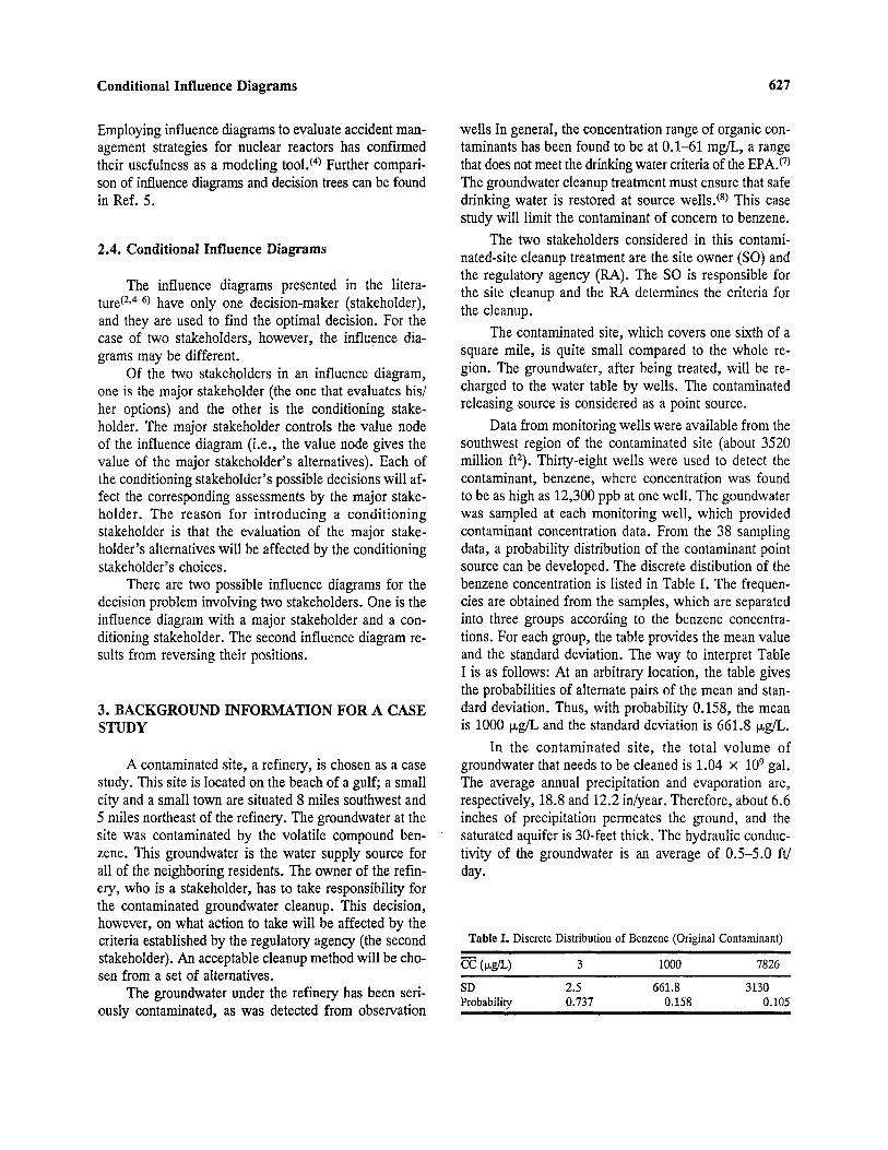
Data from monitoring wells were available from the southwest region of the contaminated site (about 3520 million ft2). Thirty-eight wells were used to detect the contaminant, benzene, where concentration was found to be as high as 12,300 ppb at one well. The goundwater was sampled at each monitoring well, which provided contaminant concentration data. From the 38 sampling data, a probability distribution of the contaminant point source can be developed. The discrete distibution of the benzene concentration is listed in Table I. The frequen- cies are obtained from the samples, which are separated into three groups according to the benzene concentrations. For each group, the table provides the mean value and the standard deviation. The way to interpret Table I is as follows: At an arbitrary location, the table gives the probabilities of alternate pairs of the mean and standard deviation. Thus, with probability 0.158, the mean is 1000 pg/L and the standard deviation is 661.8 p a .

In the contaminated site, the total volume of groundwater that needs to be cleaned is 1.04 x lo9 gal. The average annual precipitation and evaporation are, respectively, 18.8 and 12.2 idyear. Therefore, about 6.6 inches of precipitation permeates the ground, and the saturated aquifer is 30-feet thick. The hydraulic conduc- tivity of the groundwater is an average of 0.5-5.0 ft/ day.

Table I. Discrete Distribution of Benzene (Original Contaminant) - cc ( P a ) 3 1000 7826

SD 2.5 661.8 3130 Probabilitv 0.737 0.158 0.105


m m Action 4. CONSTRUCTION OF THE INFLUENCE DIAGRAMS

The stakeholders SO and RA will manage their own decisions, which will govern the final result of the contaminated site cleanup. In this case, there are two influence diagrams, and they are constructed simultaneously. One has SO as the major stakeholder and RA as the conditioning stakeholder; the other reverses the stakeholders’ positions.

An influence diagram may be constructed level by level. The structure level, including nodes and arcs, is built first, even though the data are incomplete. Then, the substructure of each node is built by defining the function level and determining the number level for every node. This method is the natural way of building influence diagrams.

For the purposes of decision-making, the arrange- ment of the structure consists of five tiers: action, value, objectives, attributes, and state. These tiers should not be confused with the levels (structure, function, and number). While the influence diagram is being developed tier to tier, the substructure is simultaneously being determined. An action tier is the decision node output resulting from a chosen alternative. Put another way, all possible alternatives are outcomes of the decision nodes. The objective tier denotes the purposes of a decision- maker’s action. The attribute tier shows factors that depend on the possible alternatives. The value of an attribute will vary according to each alternative. In some special cases, however, certain attribute(s) may not be affected by certain alternative(s). The state tier includes factors that further describe and clarify the relationship between the attribute and objective tiers.

4.1. The Basic Influence Diagrams: Action and Value Tiers

The construction of influence diagrams must begin with two tiers, action and value, which contain, respectively, decision and value nodes (Fig. 1). Influence diagrams can be identified by their value nodes (the subscript of the value indicates the, major stakeholder). For example, Fig. 1A is the influence diagram for SO, who is the major stakeholder. The choices of RA, the conditioning stakeholder, place conditions on the alternatives alvailable to SO. Figure 1B shows the reverse (i-e., RA is the major stakeholder whose alternatives are condi- tioned by the choices of SO). Therefore, Vso and V, stand for the evaluations of SO and RA in their respective diagrams. The objectives of these two corresponding

: i G f l 5--

Attribute

State

__

Objcctive

Value

(A) ( B)

Fig. 1. Conditional influence diagrams for (A) the site owner (SO) and (B) the regulatory agency (RA).

influence diagrams are different. The SO’S influence diagram (Fig. 1A) indicates a comprehensive evaluation of cleanup treatment methods given the choices of RA. Conversely, Fig. 1B shows the comprehensive evaluation of RA’s policy given the treatment methods of SO.

4.1.1. Decision Nodes SO and RA

A privately owned site has groundwater contamination and SO has to bear the cost to remediate the site to a safe level. Level 2 of the decision node SO is the action of choosing possible treatments. Two treatments are chosen as possible plans of remediation: air stripping and carbon absorption (the two methods are explained in the literature-e.g., in Ref. 9). These possible treatments constitute level 2 of this decision node.

The RA establishes the criteria of the cleanup and grants the license for the cleanup process. The decision of RA is to set a cleanup requirement, which is accom- plished at level 2 of decision node RA. The policy choices are that either 90% or 99% of the contaminants are to be removed from the groundwater; these criteria constitute leveI 3 of the decision node RA.

4.1.2. Value Nodes V,, and VRA

The performance measures (level 2) of the value nodes are chosen as dimensionless utility values, in this


case with the range [0,1]. The physical models of the value nodes are a utility function, which is employed because the stakeholder’s objective are measured in different units (e.g., individual risk, thousands of dollars, etc.) and a stakeholder may weigh these objectives dif- ferently. In order to quantify the evaluation of the different objectives, a standardized value is needed and the utility function is a good choice for this purpose.

4.2. Objective Tier

Next, the two influence diagrams, with their action and value tiers thus far defined, are further developed by inserting additional tiers (chance nodes). In order to build the utility function (level 2 of a value node), the multiple objectives need to be identified; therefore, the objective tier is considered first. In this tier, the multiple objectives of each stakeholder are described by several chance nodes that represent the variables of the utility function. These objectives may differ with each stakeholder. For SO, his cleanup objectives include cost minimization (CM), health-and-safety improvement (HSI), and environmental protection (EP). It is reasonable to assume that cost minimization is a major objective. Health- and-safety impact studies are requried by law. Also, fail- ure to comply with standards may cause both economic and political problems (e.g., with employee health in- surance and personal injury lawsuits). Environmental protection is required of the company management, and noncompliance with environmental regulations results in penalties. Because the objectives affect the value of the action, the arcs from these objective nodes point to the SO’s value node, Vso. Since these objectives depend on the possible choices of the two stakeholders, the arcs from the decision nodes point to these objective nodes.

Stakeholder RA’s objectives include minimization of adverse socioeconomic impact (MSI), in addition to EP and HSI. In this case, RA will not be responsible for the cost of the contaminated site cleanup, so cost minimization will not be an objective of RA. Each node is discussed below and the measures for each are summa- rized in Table 11.

4.2.1. Node HSI

For both diagrams, HSI is expressed as risk to an individual. The scale is logarithmic and the range is from 10-lo (utility of one) to 10’ (utility of zero). A utility function (level 2), which is the physical model of HSI,

Table 11. Measures of Objective Tier

Level 2

Performance Objective tier node measure Unit

1. Health-and-safety improvement Fatalities Individual risk

2. Environmental protection (EP) Constructed 0,1,2,3,4,S

3. Mitigate socioeconomic impact Constructed 0,1,2,3,4

(HSI)

scale

(MSI) scale 4. Cost minimization (CM) Costs M$

is used to describe the stakeholder’s attitude toward risk (e.g., risk averse, risk neutral, or risk prone).

4.2.2. Nodes EP and MSI

There is no common unit of measurement for either environmental or socioeconomic impact. In order to ana- lyze them quantitatively, constructed scales(lO) are introduced for each. These scales are defined either from 0 to 4 or 5, where 0 is the best case and 4 or 5 the worst. In building the two-component utility functions for these two constructed scales, the range of utility values is from 0 to 1. Here, each of the two-component utility functions is assumed to be linear. When the node’s value is 0 (best case), the utility is 1, and when it is 4 or 5 (the worst case), the utility is 0.

4.2.3. Node CM

The CM objective is the minimization of the cost of the cleanup treatment. In level 2, this node will be measured in dollars. Assuming a risk-neutral attitude, SO’s component utility function ranges from $1 to $10 per 1000 gal.

4.2.4. Utility Functions

The decision-makers can choose the component utility functions, such as those listed in Table 111, to describe their attitudes toward each node in the objective tier. Component functions may be risk averse, neutral, or prone.

The form of this multiobjective utility function can be assumed to be additive (linear), multilinear, or mul- tipIicative.(ll) This function is used to account for the


Table 111. Component Utility Functions

Utility Function Risk Attitude

1 - 0.5 log(WH) Averse 1 - 0.5 log(PH) Averse 1 - (CM - 1)/9 Neutral 1 1 - EP/5 Neutral 1 - MSI14 Neutral 1 - 0.5 lOg(WH) Averse 1 - 0.5 log(PH) Averse

Restriction

10-4 to 10-6

10-4 to 10-6

if 11 CM I 10 i f C M s 1 0, 1 , 2 , 3 , 4 , 5 0, 1 ,2 ,3 ,4 10-4 to 10-6

10-4 to 10-6

Node

WH PH CM

EP MSI WH PH

weights of the corresponding objectives that reflect the subjective opinion of the major stakeholder. The variables of the utility function’are the objectives (the objective node in the influence diagrams). The utility functions for each stakeholder’s objectives (in the present case study) are taken to be

k(V,,) = 0.08p(EP) + O.Sp(CM) + 0.42p(HSI)

k(V,) = 0.14p(EP) + 0.40p(MSI) + 0.46p(HSI)

(1)

(2)

The coefficients (0.08,0.50,0.40, ...) are the subjective weights for the respective objectives.

4.3. Attribute Tier

Multiple attributes result from the stakeholders’ decisions. From Ref. 10, there are several attributes that will be affected by the action. In SO’s influence diagram (Fig. lA), the choice of treatment affects the contaminant release (node CR). This node, then, is an attribute of the decision (choice of treatment). Node C, the cost of a particular treatment, is another attribute of the decision. The addition of these attribute nodes (CR and C) directly after the decision nodes is shown in the figure.

The relation between each attribute and each of the objectives must now be studied. The cost minimization (node CM) objective is influenced only by the attribute of cost (node C). The contaminant release (node CR) attribute affects the health-and-safety improvement (node HSI) objective and environmental protection (node EP). Therefore, arcs connect nodes C and CM, CR and HSI, and CR and EP. When considering treatment for CR, information regarding the initial contaminant concentration is needed. Therefore, the node for contaminant concentration (CC) is introduced to influence the node CR. The CC node, which is not influenced by other factors (hence no arc points to it), is called a source node.

In RA’s influence diagram (Fig. lB), the policy

actions are associated with the following attribute nodes: contaminant release (CR), manpower (M), and treatment effectiveness and reliability (E). Therefore, arcs from the attributes point to the corresponding objective nodes.

4.3.1. Node C

In the literature,(”-) the costs of air stripping and carbon absorption are analyzed with 95% contaminant removal. Here, costs for the same treatments are evaluated for 90% and 99% contaminant removal and are shown on Table IV for each alternative pair.

4.3.2. Node CC

The function level of node CC contains the original contaminant concentration distribution.

4.3.3. Node CR

The value of the CR node is the contaminant-effluent distribution after groundwater treatment. The performance measures of the node are the concentration measures corresponding to the effluent media, such as water or air. The physical model of the node deals with release pathways of the contaminant. The physical model of the treatment will be studied later after relevant nodes of release pathways are discussed. In defining the substructure (level 2) of node CR, the model of the air- stripper design defines the function level, since it affects the effluent releases to the atmosphere.

4.3.4. Nodes M and E

In RA’s influence diagram, manpower (M) represents the number of employees required by a particular treatment. If this number is large, more people will be exposed to contaminants. In other words, the value of

Table IV. Costs of Groundwater Treatments

SO’s treatment RA’s policy alternatives requirements (%) Cost (M$)

Air stripping 90 Air stripping 99 Carbon absorption 90 Carbon absorution 99

0.50 2.50 1.40 6.20

Conditional Influence Diagrams 63 1

objective HSI will depend on node M, the number of the employees required.

Treatment effectiveness (E) refers to the reliability of the treatment. A treatment may fail to reach the des- ignated cleanup level, which may cause contaminant releases. Even though the amount of the. released contaminant may not seriously affect human health, the public perception of this event may be very negative. Therefore, it will affect the objective node MSI of RA's influence diagram.

The performance measures (level 2) of the two nodes are constructed scales. The range of both scales is from 0-4. For these constructed scales, the physical model is defined as a scale measure. For example, the highest value for effectiveness is 4, which is a function value for the E node. The data for these constructed scales may be obtained from experts hired by each stakeholder. Table V shows the quantitative measures and parameters about the attribute nodes (level 2).

4.4. State Tier

In order to describe the connection between attributes and objectives in more detail, state nodes are introduced. For example, the objective of health-and-safety improvement (HSI) depends on workers and public health effects, (WH) and (PH) respectively. Arcs from the nodes WH and PH connect them to the HSI node. The attribute, contaminant release (CR), affects the release pathways in the air and groundwater. Therefore, nodes that describe the air and water pathways, AP and WP, depend on the node CR. For example, some of the contaminants may leave a residue in the groundwater or may release toxins into the atmosphere after being treated. The arcs connect node CR and the nodes AP and WP. Because humans are exposed to contaminants through air and water, the nodes AP and WP are related to, and connected with, the nodes WH and PH. Groundwater hydrology provides important information for evaluating

Table V. Measures of Attribute Tier

Level 2

Performance Attribute measure Unit

1. Contaminant release (CR) Concentration Psn 2. Cost of treatment (C) Cost M$ 3. Manpower (M) No. of people Person 4. Effectiveness (E) Constructed scale 0,1,2,3,4

contaminant propagation along the water path. Because groundwater data are uncertain, a chance node for groundwater hydrology (GH) is added to point to the node WP. Node GH, having no arc pointing to it, is a source node (as was CC earlier). The structure levels of the final influence diagrams for SO and RA are shown in Fig. 1.

4.4.1. Node CR

A physical model is needed to provide input values for nodes AP and WP. Air stripping, a process utilized to remove volatile compounds from groundwater, is widely accepted for remedial work on groundwater contamination. It involves a packing tower where contaminated water enters at the top and flows downward through the packing, while the air stream flows upward picking up volatile compounds. Water is collected at the bottom and pumped to its final destination, while the air exits at the top of the tower and is dispersed, along with the volatiles, into the atmosphere. The model involves the design of the packing tower, in which two variables are considered, tower height and the air:water ratio. The packing height is given by(9)

where

R = H - G/L * P,

and

Z, = packing height (m) L = liquid loading rate (m3 m-2 sec-'),

KLu = mass transfer coefficient (sec-l), Ci, = influent concentration (consistent units),

= effluent concentration (consistent units), H = Henry's law constant (atm m3 H20 m-3

G = gas loading rate (m3 m-2 sec-2), P, = operating pressure (= 1 atm).

Here, H is 80 for benzene and Cin/Ceff is determined by RA's decision to remove either 90% or 99% of the contamination. This ratio will be 10 for 90% and 100 for 99%. The choice of G will affect the tower height. The lower the gas loading rate, the higher the packing height.

The significance of the tower height design is that it determines the exposure rates to the workers and to the public [see Eq. (4) below]. The tower height and effluent contaminant concentration will serve as input to

C,,

air),


the node AP. The design of carbon absorption will not be discussed, since it will not affect the air pathway.

4.4.2. Node AP

Propagation of contaminants is estimated by a point- source model, which is the function (level 2) of node AP. The coordinate axis, y , points as the wild direction.(13) We have

where C (x, y , 0) is air contaminant concentration on the ground at the position (x, y ) , Z, is the packing height (assumed to be appropriately equal to the tower height) of the air stripper, u$ = 2Dj/p, (m’) and 4 = 2D3/ p (m2), p, is the wind speed at all directions, Q is the strength of the emission source (g/sec), and D, and D, are mass diffusivity constants. In the case study, the value of p, is 3 m/sec, a, is 25, and a, is 13.

4.4.3. Node WP

In describing the substructure of the node WP, a model in the form of differential equations describes the movement of the water and the contaminants under- ground. The contaminant concentration is calculated using a model of contaminated groundwater migration. The computer code CONMIG(14), which is based on ideal aquifer and solute conditions, is used. The code contains the following assumptions: negligible solute-injection rates in relation to groundwater flow rate, steady-state groundwater flow, negligible difference in density and viscosity between recharge and native water, uniform groundwater velocity in one direction, horizontal scale of migration much larger than aquifer thickness, flow field is horizontally two-dimensional (2D), and contaminants are quickly mixing vertically. The equation governing contaminant migration in uniform 1D flow from a point source without absorption or decay is

C = 1.064 10-2CoVc exp

where

C C,

V,

= change of water concentration ( p a ) = difference in concentration between in-

= volume of injected mass (L) jected and native water

x y y =time (day) V,

A, = longitudinal dispersivity (m) A T = transverse dispersivity (m) m = aquifer thickness (m) n = aquifer effective porosity

= coordinate along the flow direction (m) = coordinate along the vertical direction (m)

= seepage velocity without adsorption (m/ day),

Equation (5) represents the function level of the node WP, while the information about the parameters of Eq. ( 5 ) is the third level.

In the case study, actual porosity of the aquifer is 0.3, and the effective porosity is 0.2. Aquifer longitudinal and transverse dispersivities are, respectively, 30 m and 3 m. These values are used in the code CONMIG.

4.4.4. Node GH

Groundwater hydrology data (Section 3) involve basic information about the propagation of contaminants through groundwater and give input for the water pathway model. Node GH is, therefore, connected with node WP.

4.4.5. Nodes WH and PH

In the substructure of these nodes, the exposure model estimates the human dose of a contaminant based on its concentration and describes the rate of contaminant absorption from various pathways.

Because the contaminant exposure dosages from the air and water paths are independent, the exposure to human beings will vary. For the individual worker, the dose is

w H = A P + W P (6) that is, the worker suffers contaminant exposure from both the water and air. For a member of the public (individual risk), the dose is

PH = max(AP,WP) (7) that is, because the winds are blowing in a direction opposite to the groundwater flow, an individual can only be exposed to one of the two paths. Equations (6) and (7) are the functions of nodes WH and PH, where AP and WP stand for the values of the corresponding nodes.

The risk range for both the workers and the public is to which corresponds to the daily exposure concentrati~n(’~) of benzene of from 1 to 100 p a . This relationship describes the quantitative function from the


exposure dose to the individual’s risk. Then, the risk can be incorporated into the component utility function to find the utility of the node. (The units are probability of deaths per year.) However, there is a one-to-one correspondence between exposure dose and utility. Therefore, the utility value can be determined from a given exposure dose. The relationship between utility and exposure dose for WH and PH is shown in equation form by entries in Table 111.

Health-and-safety improvement is assumed to be related to the health of workers and the public as follows:

p(HS1) = 0.8p(WH) + 0.2p(PH), for SO (8)

p(HS1) = OSp(WH) + 0.5p(PH), for RA (9)

These equations are utility functions, p, where the variables correspond to the utility values of the respective nodes. The coefficients of the variables are the attitudes of the stakeholders. For example, in Eq. (9), RA will pay equal attention to the health of workers and the public.

5. EVALUATION OF INFLUENCE DIAGRAMS

After setting up the levels (structure, function, and number), the next step is to evaluate them. The purpose is to transform the decision vectors into the value matrix, where each decision vector is the set of a stakeholder’s alternatives.

The influence diagrams in Fig. 1 are evaluated for the given decisions and data. An alternative pair comprises one decision each from two alternatives of stakeholders SO and RA. Because each stakeholder has two alternatives, the total possible number of alternative pairs is four.

Air-stlipping-9#%-removed pair: SO chooses the air stripper as the cleanup method and RA sets the cleanup level at 90% of the volatiles removed. The direct result of this alternative pair is that 10% of contaminants remain in the groundwater and 90% of the contaminants are released into the atmosphere.

Air-stnpping-99%-removed pair: This decision pair will cause 99% of the contaminants to be removed. Compared with the former pair, 10% more contaminants wilI propagate through air and 90% fewer contaminants will remain in the groundwater.

Carbon-absorption-9O%-removed pair: This decision pair applies carbon-absorption treatment to the water with RA’s requirement of 90% of contaminants removed before it is recharged to groundwater. This decision pair will not cause any volatile contaminants to

be released into the atmosphere. However, the effectiveness of the method may be reduced when the acti- vated carbon is polluted.

Carbon-absorption-99%-removed pair: This pair is similar to the previous pair except that fewer contaminants are allowed to be recharged into groundwater.

5.1. Evaluation of Source Nodes CC and GH

After the alternative pair is identified, the values of the attribute nodes can be considered as initial input data for the rest of the influence diagram. (The two decision nodes will be discarded after determination of the alternative pair.) The source chance nodes, CC and GH, were estimated during the construction of the diagrams. The value of CC is a random variable (listed in Table I), and the value of GH is the groundwater data (described in Section 3). Therefore, the other nodes can be estimated systematically from values of CC, GH, and the two decision nodes.

5.2. Evaluation of Node CR

The ratio of benzene released into the air is put into Eq. (3), which is used to design the air-stripping treatment for groundwater. From Eq. (3), the packing height is 30 m, According to the example alternative pair, air stripping removes 90% of the benzene from the groundwater, leaving 10% of it to be recharged back into the water table. The value of CR comprises two parts, the water path and the air path. The removed benzene is released into the atmosphere. The benzene distribution does not vary from node CC to node CR, because of the assumption that the distribution remains the same as water is pumped during treatment. After 90% of the benzene is removed from the groundwater, the concentration distribution for the water path is 0.3, 100, and 782 pg/L with probabilities, respectively, of 0.737, 0.158, and 0.105. The distribution for the air path is 24, 160, and 300 mg/sec with the respective probabilities of 0.737, 0.158, and 0.105.

5.3. Evaluation of Nodes W P and AP

The propagation of benzene in the groundwater is estimated by using the computer code CONMIG. In this example, the code determines that the concentration of benzene near the water well for workers will be 10% less than that from the contaminant source. The value


of WP to workers’ exposure is the distribution that is shown in Table VI.

The calculation of the exposure distribution from the air path is similar to the water path. For the air path, the concentration is given by Eq. (4). The value Q comes from the air path output of CR. The distribution of Q is 0.024, 0.16, and 0.30 (g/sec) with respective probabilities of 0.737, 0.158, and 0.105. The results of Eq. (4) are also shown in Table VI. The distribution, represent- ing the highest concentrations on the ground, reflects conservative risk estimates. The same king of calculation is applied to node AP as was used for WP. The last column shows the value of AP.

5.4. Evaluation of Nodes WH and PH

The times for the benzene to reach humans will be different for the air and water paths, and their distribution will be assumed as independent. The accumulated exposure rate to workers is computed from the exposure distribution of the water and air paths. For convenience, the exposure dose from the air path is converted to the equivalent dose in p a . Using Eq. (6), we find that the accumulated rate is the mixed sum from the air and water distributions. Therefore, the fifth column of Table VII is the sum of possible air and water concentrations. The last column is the product of columns two and four. The bottom row of the table is the expected dose to workers. Finally, the value of node WH is found by using the component utility function for WH in Table 111. The utility is 0.407.

The manner of evaluating node PH is similar to that of node WH, the only difference is that Eq. (7) is used instead of Eq. (6). For node PH, the exposure dose to an individual from the water path is 1.954 p&, and the eqivalent exposure dose from the air path is 0.740 kg/L. These two values become the variables in Eq. (7), from which the result is the maximum of the two values. The result is 1.954 p a . From the component utility

Table VI. Contaminant Propagation by Water and Air Paths after Treatment by Air-Stripping Method (90% of Hazards Removed)

Concentration Distribution

WP (Fd)

0.0 10. 78. 0.0 0.56 4.50

0.737 0.158 0.105 0.737 0.158 0.105

Table VII. Risk Expectation After Treatment by Air-Stripping Method (90% of Hazards Removed)

WP AP WH

Conc. Conc. Conc. (I@) Prob. (kglrn’) Prob. (&L) Prob.

0 0.737 0 0.737 0 0.544 5.6 0.116

10.0 0.116 10 0.158 0.56 0.158 15.6 0.025

45.0 0.077 78.6 0.077

78 0.105 4.50 0.105 83.6 0.017 55.0 0.017

123.0 0.011 Expected dose: 15.4

function for PH in Table 111, the utility is 0.855. Finally, using Eq. (8), we get the utility of HSI as 0.495.

5.5. Evaluation of Node C

Based on the data of this example, the cost to clean up the groundwater by the air-stripping method is $0.5 M (Table V).

The node AP, which affects the value of objective node EP, comes from the evaluation given previously. Then, nodes CM and EP are estimated as, respectively, $0.5 M and $1 M. The contaminant release after treatment causes the pollution to be 1 on a constructed scale from 0-5 (Table 11).

These values of CM in millions of dollars and EP on the constructed scale are put into physical models [i.e., the utility functions (Table 111) of the objective nodes CM and EP], in which the results are the utilities 1 and 0.8, respectively.

5.6. Utility Analysis

After the values of the objective nodes are obtained, the value of the alternative pair can be calculated from these objective values by the utility functions of the value node [Eqs. (1) and (2)]. The values of the objective nodes are the component utilities (Table 111). We sub- stitute the component utilities of EP, CM, and HSI (0.80, 1.00, and 0.573) as variables in Eq. (1). The result of the computation (0.77) is the value of the decision pair for stakeholder SO. Correspondingly, RA’s evaluation can be computed by substituting the component utilities (objective values) EP, MSI, and HSI as variables in Eq.


(2). As a result, the value (0.50) of RA’s influence diagram is found. For each alternative pair, there are two values, one each for SO and for RA.

This method can be repeated for every alternative pair. Evaluating the influence diagrams proceeds step by step from the decision nodes to the value nodes. After the evaluation of each alternative pair is obtained, the numerical results should be put into a bimatrix (Table VIII).

RA to choose 99% cleanup and the SO to choose air stripping as the cleanup method.

However, a closer examination of Table VIII re- veals that the expected utility pair (0.80,0.73) represents decisions that are more beneficial to each of the stakeholders (each expected utility is greater than its corresponding value in the equilibrium solution). This means that, if the two stakeholders agree to change their decisions (the RA to 90% cleanup and the SO to carbon absorption), they will both be better off. This requires cooperation and mutual trust between the stakeholders.

6. GAME THEORY ANALYSIS 7. CONCLUDING REMARKS

After obtaining the bimatrix, we proceed to reach the optimal decision by using game theory.(16J7) In this work, the game, which has two players (SO and RA), is a probabilistic game. Because their motivations do not include dominating the opponent, the two stakeholders are not considered to be competing players. From the bimatrix of the alternative evaluation, it is seen that the game is nonzero sum (the reward of one stakeholder is not equal to the loss of the other).

If each stakeholder makes his own decision without considering his opponent’s payoffs, conflict may result. First, the SO’S payoffs are considered. From Table VIII, the SO’s alternative “carbon absorption,” is better than air stripping if RA chooses the alternative that 90% of the benzene should be removed. However, air stripping is better than carbon absorption if 99% of the benzene has to be removed from the groundwater. As a result, the SO’s decision will depend on the RA’s decision.

We now turn to the RA’s payoffs. Comparing the two columns of the RA’s outcomes, no matter what alternative is chosen by the SO, the alternative of 99% cleanup is better than the alternative of 90% cleanup and will, therefore, be chosen. This decision of the RA will force the SO to choose the alternative with the best utility. From the table, it is easy to see that the SO will choose the air-stripping method.

Thus, we see that, when each stakeholder only looks after his own interest, the equilibrium solution is for the

This paper has introduced the concept of conditional influence diagrams and their use as an alternative to decision trees in risk management. This allows the decision options of each stakeholder to be evaluated by assuming that the other stakeholder acts in a given manner. Given the results in the bimatrix, the stakeholders can search for an “optimaly’ solution that would be acceptable to both, Their willingness to cooperate is an important element in their search. The methods of game theory are useful in this regard.

While the analysis presented here provides useful insights into the problem of multiple stakeholders, ex- tending this approach to more than two stakeholders and/ or to more than two decision options for each is not straightforward. In those cases, searching for the optimal solution becomes very complex, even with the use of formal metagame theory. This is to be expected, since the problem of many stakeholders is, in general, a very complicated one.

ACKNOWLEDGMENTS

We thank Joan George, Stephen Chien, and David Bell for helping to edit the manuscript. This work was supported in part by the Risk and Systems Analysis for the Control of Toxics (RSACT) program at UCLA.

REFERENCES Table VIII. Bimatrix of Decision Game

RA’s alternatives

SO’s alternatives- 90% 99%

Air stripping 0.77, 0.50 0.76, 0.68 Carbon absomtion 0.80. 0.73 0.71. 0.90

1. J. Massmann and R. A. Freeze, “Groundwater Contamination from Waste Management Sites: The Interaction Between Risk- Based Engineering Design and Regulatory Policy. 1. Methodol- ogy,” Water Resources Research 23, 351-367 (1987).

2. S. Holtzman, Intelligent Decision Systems (Addison-Wesley Pub- lishing Company, Inc., Reading, Massachusetts, 1989) pp. 5 6 77.


3. Y. Y. Haimes, D. Li, and V. l’ulsiani, “Multiobjective Decision- Tree Analysis.” Risk Analysis 10, 111-129 (1990).

4. M. fae and G. Apostolakis, ‘“The Use of Influence Diagrams for Evaluating Severe Accident Management Strategies,” Nuclear Technology 99, 142-157 (1992).

5. H. Call and W. Miller, “A Comparison of Approaches and Im- plementations for Automating Decision Analysis,” Reliability En- gineering and System Safety 30, 115-162 (1990).

6. R. D. Shachter, “Evaluating Influence Diagrams,” Operations Research 34, 871-882 (1986).

7. “Superfund Public Health Evaluation Manual” (U.S. Environ- mental Protection Agency report EPA/540/1.86/060, PB87-183125, 1986).

8. “Ground Water Handbook” (U.S. Environmental Protection Agency report EPA/625/6-87/016, 1987).

9. E. K. Nyer, Groundwater Treatment Technology (Van Nostrand Reinhold Co., New York, 1985) pp. 47-78.

10. M. W. Merkhofer and R. L. Keeney, “A Multiattributte Utility Analysis of Alternative Sites for the Disposal of Nuclear Waste,” Risk Analysis 7, 173-194 (1987).

11. R. L. Keeney and H, Raiffa, Decisions with Multiple Objectives:

Preference and Value Tradeofls (Wiley & Sons, New York, 1976),

12. “Initial Study and Proposed Negative Declaration for the Pro- posed North Hollywood-Burbank Aeration Facility Project” (Los Angeles Department of Water and Power report, 1986), pp. 1- 39.

13. R. Ranchoux, “Determination of Maximum Ground Level Con- centration,” J. Air Pollution Control Assoc. 26, 1088-1089 (1976).

14. W. C. Walton, Analytical Groundwater Modeling: Flow and Con- taminant Migration (Lewis Publishers, Chelsea, Michigan, 1989),

15. J. J. Cohrssen and V. T. Covello, “Risk Analysis, A Guide to Principles and Methods for Analyzing Health and Environmental Risks” (US. Department of Commerce report, Springfield, Vir- ginia, 1989), pp. 55-98.

16. G. Owen, Game Theoiy (Academic Press, Inc., Orlando, Florida,

17. N. Howard, Paradoxes of Rationality: Theoiy of Metagames and Political Behavior (MIT Press, Cambridge, Massachusetts, 1969), pp. 50-78.

pp. 131-281.

pp. 39-44.

1982), pp. 1-190.

Conditional Influence Diagrams in Risk Management

Documents

Transcript of Conditional Influence Diagrams in Risk Management