BR

ICS

RS

-98-46Larsen

etal.:C

lockD

ifferenceD

iagrams

BRICSBasic Research in Computer Science

Clock Difference Diagrams

Kim G. LarsenCarsten WeiseWang YiJustin Pearson

BRICS Report Series RS-98-46

ISSN 0909-0878 December 1998

Copyright c© 1998, BRICS, Department of Computer ScienceUniversity of Aarhus. All rights reserved.

Reproduction of all or part of this workis permitted for educational or research useon condition that this copyright notice isincluded in any copy.

See back inner page for a list of recent BRICS Report Series publications.Copies may be obtained by contacting:

BRICSDepartment of Computer ScienceUniversity of AarhusNy Munkegade, building 540DK–8000 Aarhus CDenmarkTelephone: +45 8942 3360Telefax: +45 8942 3255Internet: BRICS@brics.dk

BRICS publications are in general accessible through the World WideWeb and anonymous FTP through these URLs:

http://www.brics.dkftp://ftp.brics.dkThis document in subdirectory RS/98/46/

Clock Difference Diagrams

Kim G. Larsen Carsten WeiseBRICS∗, Aalborg University, Denmark

Yi Wang Justin PearsonDepartment of Computer Systems, Uppsala University, Sweden

December, 1998

Abstract

We sketch a BDD-like structure for representing unions of simple con-vex polyhedra, describing the legal values of a set of clocks given boundson the values of clocks and clock differences.

1 Introduction

The basic problem we are trying to tackle is the combination BDD’s and DBM’s(difference bound matrices) in order to allow completely BDD-based approachto the verification of continuous real-time systems. Early appraches in thisdirection are [WTD95] and [Bal96]. Another inspiration for this work comesfrom [ST98]. Some of the ideas come from the implementation of a decisionalgorithm for timed bisimulation ([WL97]).

2 Definition of CDD’s

We assume a finite set of real-valued clocks C = {X1, . . . , Xk}. We are interestedin a data structure to represent and manipulate sets of possible values of theseclocks. In particular, we shall confine ourselves to sets being the finite unions ofsimple convex polyhedra. The simple convex polyhedra are described by boundson the individual clocks and clock differences of the form Xi −Xj . These kindof sets occur typically in the analysis of real-time systems when modelled astimed automata.

∗BRICS: Basic Research in Computer Science, Centre of the Danish National ResearchFoundation

1

For a uniform treatment, we assume an additional clock X0 which always hasvalue zero. Then the absolute value of clock Xi is referred to as Xi −X0.

Let V := {v : C → R} be the set of clock valuations. Then any polyhedradescribed by clock differences is a subset of V .

A clock constraint has the form m ≤ Xi −Xj ≤ n, where i, j ∈ {0, . . . , k} andm,n are integers. Instead of ≤ also < can be used in the lower and the upperbound. We will always require i > j, as m ≤ Xi − Xj ≤ n is the same as−n ≤ Xj −Xi ≤ −m. Note that for i = j, we always have 0 ≤ Xi −Xj ≤ 0.

For any constraint, we call the pair (i, j) the type of the constraint. It is obviousthat in any description of a convex set, at most one constraint per type is needed.As mentioned before, we always assume i > j. We define a linear ordering on thetypes, which we denote by v . This ordering is the “reversed lexicographical”ordering, i.e. (i, j) v (i′, j′) iff either j < j′ or j = j′ and i ≤ i′.In the following, any set describable by a conjunction of clock constraints willbe called a zone. A federation is any finite union of zones.

We will now define a data structure called clock difference diagrams (short:CDD) which can be used to represent federations. The basic idea is derivedfrom BDD’s, but adapted to the fact that our variables do not range over asimple two-valued alphabet, but over the real numbers instead.

While the idea of a BDD is that of a decision-diagram branching on the differentsingle values of the variables of a term, a CDD node branches with respect tointervals of the reals for a given clock difference, i.e. a CDD node is associatedwith the type of the clock difference for which it is testing. The size and thenumber of the intervals is not fixed. However there can only be a finite numberof intervals, and they must be compatible with the clock constraints (i.e. theyare intervals with integer bounds, and any bound can either be included or not).Remember that a major idea in BDD’s is that of sharing identical substructures,therefore a BDD is in fact an acyclic graph rather than a tree, and so will bethe CDD’s.

In the general case we will not require that the intervals belonging to one nodeare disjoint. We will however show that there is an easy way to obtain disjointintervals if needed, as most of our operations will require disjoint intervals.

The finite number of intervals within a node is assured by not differentiating be-tween points when a clock exceeds a given maximal value M . Thus the intervals(+M,+∞) and (−∞,−M) cannot be further partitioned. If an operation yieldsa subinterval intersecting one of these, then this subinterval must be extendedwith the whole interval.

There are two special nodes called True and False. They are used to indicatethat along a certain path all valuations belong to the federation or do not belongto the federation. In general, our graphs will be complete, i.e. for any valuationthere is at least one path leading to either a True or a False node.

Thus a CDD consists of the following kinds of nodes:

2

• end-nodes, which are either True or False, and which have no successor,

• inner nodes, which for a fixed type branch to nodes for different constraints(intervals) of this type

���������

���������

���������

���������

������������

��������

���������

���������

���������

���������

����

����

1

y

1 2 3 4 4 6x

1

2

3

1

y

1 2 3 4 4 6x

1

2

3

1

x1 3 4 6

1 3

y

1 2 3 4 4 6x

1

2

3

y

x

y

x

y

x− y

1 2 3 4

1 3 2 4

0 2

0 1 2 3

0

0 1

Example 2

Example 1

Example3

Figure 1: Three Simple Examples

Example 1, 2 and 3 as given in Figure 1 are simple examples of CDD’s. Notethat instead of True we use boxes with a 1 inside (like in BDD’s). We havealso not drawn the False end-nodes. Remember that there are many different

3

ways to represent a federation as a CDD. Note also that Example 1 uses sharingof the nodes of type (2, 0), i.e. those giving constraints on Y .

A clock difference diagram is defined as a directed, acyclic graph, which has

• a node called the start node from which all nodes of the graph are reach-able,

• inner nodes written as ((i, j), (I1, T1), . . . , (Iq, Tq)) where (i, j) is the typeof a constraint, the In are intervals of the real numbers, and the Tn areCDD’s again. We require completeness, i.e.

⋃n∈{1,... ,q} In = R.

• end-nodes which are either True or False.

Note that a node in a CDD defines a subgraph of all nodes reachable from thisnode. This subgraph can be seen as a CDD with the current node as the startnode. We will identify a node and the sub CDD defined by it.

The interpretation of such a CDD should now be obvious: If we take a pathfrom the start node to an end-node, this path describes a zone given by theconjunction of the clock constraints on this path. A clock constraint on a pathis the constraint representing the interval which we had to choose to follow thebranches building the path. If the path ends in True, then all valuations ofthis zone belong to the federation. The CDD represents the union of all zonesdescribed by paths leading to True.

In order to formalize the semantics of CDD’s, we use the following notation:

• given a type (i, j) and an interval I of the reals, then I(i, j) denotes theclock constraint having type (i, j) which restricts the value of Xi −Xj tothe interval I.

• given a clock constraint φ and a valuation v, by φ(v) we denote the appli-cation of φ to v, i.e. the boolean value derived from replacing the clocksin φ by the values given in v.

Note that typically we will use the notation jointly, i.e. I(i, j)(v) expresses thefact that v fulfills the constraint given by the interval I and the type (i, j).

As an example, if the type is (2, 1) and I = [3, 5), then I(i, j) would be theconstraint 3 ≤ X2 −X1 < 5. For v where v(X2) = 9 and v(X1) = 5.2 we wouldfind that I(i, j)(v) is true, while for v′ with v′(X2) = 3 and v′(X1) = 4 we wouldhave I(i, j)(v′) is false.

Using this, we can formally define the semantics of a CDD by

• [[True]] := V ,

• [[False]] := ∅,

4

• [[((i, j), (I1, T1), . . . , (Iq , Tq))]] :=⋃n∈{1,... ,q}{v ∈ [[Tn]]|In(i, j)(v) = True}

Note that this semantics is defined so that any valuation v for which there is apath to True in the CDD will be part of the set described by the CDD. Thisincludes the case where there might be another path for v leading to a zero,which seems rather counter intuitive. In fact, the False end-nodes could beclipped from the CDD’s without doing harm. They are mainly used here to makesome formal treatment more easy (e.g. definition of union and intersection). Agood implementation would not need to store them.

2.1 Reducing Redundancy

A major point in the coding is to get rid of redundancies as much as possible.Therefore we require orderedness and disjointness.

Orderedness: Remember that we assume some ordering on the types. Wefurther assume that True and False have a type. Their types are the maximalelements in the order, i.e. they are larger than any other type. Given a node Nof a CDD, we can now speak of the node’s type denoted by type(N). We saythat a CDD is ordered if for any node T = ((i, j), (I1, T1), . . . , (Iq, Tq)) it is truethat for all n ∈ {1, . . . , q} that type(T ) v type(Tn) and type(T ) 6= type(Tn).This means that along any path, the types are increasing, and that no typeoccurs twice along the path.

In the following, we will always assume that our CDD’s are ordered. All ouroperations will keep orderedness. Note that in fact Examples 1 to 3 were alreadyordered.

Disjointness: We say that a CDD T = ((i, j), (I1, T1), . . . , (Iq, Tq)) is disjointif all intervals are disjoint, i.e. for all n,m ∈ {1, . . . , q}, from n 6= m it followsthat In∩Im = ∅, and if all sub CDD’s Tn are disjoint as well. The CDD’s True

and False are disjoint by definition.

Basically we will always require disjointness. However some of our operationswill destroy disjointness. But there is a simple way to go from an ordered CDDto a disjoint ordered CDD which will be explained later.

Figure 2 shows how to represent Example 2 as a disjoint CDD. It also gives adifferent graphical representation of the set fitting more the CDD representation.

Sharing: In order to reduce memory for the storing of a CDD we want to haveas much sharing of subgraphs as possible. So within a CDD we require that ifthere are two subgraphs which are isomorphic then they should be the same.It is of course always possible to construct a maximally shared CDD from anygiven CDD.

5

������

������

��������

��������

������

������

11 2 3 4 5

1

2

3

4

y

x

1 2 3 4x

y

Figure 2: Enforcing Disjointness

We can generalize this rule for sharing. If there are two neighboring or over-lapping subintervals in a node which point to the same subgraph, then the twointervals can be replaced by their union, pointing to the subgraph. Also, if anode contains (−∞,+∞) as the only interval, this node may be removed byredirecting all pointers to the node to its subgraph.

2.2 Normal Form

Certain operations on CDD’s require the CDD to be in a defined normal form,analogously to the case of DBM’s for zones. A CDD in normal form is requiredto have maximal sharing, and be ordered and disjoint. Further we require thatalong any path leading to True, the constraints must be the tightest possible,i.e. if we replace a constraint along a path by a tighter one, then the semanticsof the CDD changes.

We will see further down how to obtain a CDD in normal form from an orderedand disjoint CDD.

3 Operations on CDD’s

The most simple operations on CDD’s are union and intersection. Assume twoCDD’s TA, TB given, which are ordered and disjoint. Then the CDD TC =TA ∪ TB is constructed recursively in the following way:

• if TA = False, then TC := TB,

• if TA = True, then TC := True,

• if TA 6∈ {True, False} and type(TA) 6= type(TB), assume w.l.o.g. type(TA) vtype(TB). Let TA = ((i, j), (I1, T1), . . . , (Iq , Tq)), thenTC := ((i, j), (I1, T1 ∪ TB), . . . , (Tq, Tq ∪ TB)).

6

• if TA 6∈ {True, False} and type(TA) = type(TB), thenlet TA = ((i, j), (I1, T1), . . . , (Iq, Tq)) and TB = ((i, j), (J1, S1), . . . , (Jr, Sr)).Then

TC := ((i, j), (I1 ∩ J1, T1 ∪ S1), (I1 ∩ J2, T1 ∪ S2), . . . , (I1 ∩ Jr, T1 ∪ Sr),(I2 ∩ J1, T2 ∪ S1), . . . ,. . . (Iq ∩ Jr, Tq ∪ Sr))

where empty intervals can safely be discarded.

Note that this operation keeps orderedness and disjointness. Sharing can bemaintained as well using the same dynamic methods as with BDD’s.

The intersection is basically the same, where only the non-recursive step has tobe adjusted. The CDD TC = TA ∩ TB is constructed by

• if TA = False, then TC := False,

• if TA = True, then TC := TB,

• else replace Tn ∪ Sm everywhere in the above by Tn ∩ Sm.

3.1 Enforcing Disjointness

Given these basic operations, it is now easy to see how to enforce disjointness.Assume a CDD TA = ((i, j), (I1, T1), . . . , (Iq, Tq)) where Iq−1∩Iq 6= ∅. Then theCDD T = ((i, j), (I1, T1), . . . , (Iq−1, Tq−2), (Iq−1\Iq, Tq−1), (Iq\Iq−1, Tq), (Iq−1∩Iq, Tq−1 ∪ Tq)) will have the same semantics, but the overlap between the lasttwo intervals is gone. Applying this iteratively to all pairs of overlapping in-tervals and then recursively to all sub-CDD’s will yield a disjoint CDD. Notethat the union operation on CDD’s required here does not destroy disjointness,guaranteeing termination.

Figure 2 shows how Example 2 looks like after enforcing disjoint intervals.

3.2 Setting clocks and letting time pass

Two very important operations in the analysis of timed automata, which weare aiming at, is the setting of a clock and letting time pass. Note that forthese operations we need to assume normal form of the CDD. Note that theseoperations are mainly generalizations of their simpler DBM counterparts (wherethey require canonical form).

Setting a clock Xi (i 6= 0) to a constant c is done by replacing intervals in nodes.All intervals describing values of the clock Xi itself now become just [c, c], so asubgraph

((i, 0), (I1, T1), . . . , (Iq, Tq))

7

is replaced by

((i, 0), ([c, c], T1), . . . , ([c, c], Tq))

The difference between Xi and another clock Xj is then the difference between 0andXj minus the new value c ofXi. Note that subgraphs ((i, j), (I1, T1), . . . , (Iq, Tq))where j 6= 0 resp. ((j, i), (I1, T1), . . . , (Iq, Tq)) are reached by going through aninterval I for type (j, 0), due to orderedness. This interval gives the differencebetween Xj and zero. Replacing is done by changing the subgraphs to

((i, j), (c− I, T1), . . . , (c− I, Tq))

resp.

((j, i), (I − c, T1), . . . , (I − c, Tq))

where c − I and I − c are defined as extensions of normal subtraction, i.e.c− I := {c− x | x ∈ I} and I − c := {x− c | x ∈ I}.

1 2 3 4 5

1

2

3

4

x

y − x

y

[ ] ][

] ] [ ] [ [

1 2 3 4

2 2 2

0 1 -1 0 -2 -1

1

Figure 3: Setting Y to two

Figure 3 shows how Example 2 looks like after setting Y to two. Note thatto do this correctly, it is necessary to make Example 2 disjoint and put it intonormal form (as seen in Figure 2 and 6). However, the result is not the mostcompact form for this federation. Additional rules could be defined to gain amore compact form.

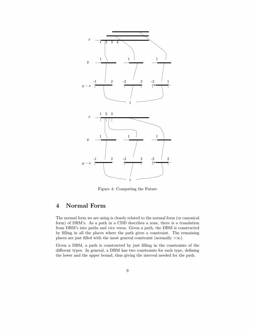
The future of a CDD is also computed straight forward by removing the upperbounds on all clocks, so ((i, 0), (I1, T1), . . . , (Iq, Tq)) becomes ((i, 0), (I ′1, T1), . . . , (I ′q , Tq))where I ′n := (k,∞) if k was the strict lower bound of In, and I ′n := [k,∞) if kwas the non-strict lower bound of In. Figure 4 and 5 gives an example.

In both cases disjointness is destroyed, but can be regained using the methodexplained in the previous section.

8

x

y

y − x

1 1 1

-1 2]

-2 2[ ] [

-2[

1

1 2 3

[ [ ]

2

x

y

y − x

1 2 3 4

1 1 1

-1 2]

-2 2[ ] [

-2 1[

1

Figure 4: Computing the Future

4 Normal Form

The normal form we are using is closely related to the normal form (or canonicalform) of DBM’s. As a path in a CDD describes a zone, there is a translationfrom DBM’s into paths and vice versa. Given a path, the DBM is constructedby filling in all the places where the path gives a constraint. The remainingplaces are just filled with the most general constraint (normally +∞).

Given a DBM, a path is constructed by just filling in the constraints of thedifferent types. In general, a DBM has two constraints for each type, definingthe lower and the upper bound, thus giving the interval needed for the path.

9

��������

��������

��������������������������������������������������������

��������������������������������������������������������

1 2 3 4

1

2

3

4

1 2[[

-1 2

] ] [ ]

-2 2

1

x

y

y − x

1 1

Figure 5: Computing the Future

To bring an arbitrary ordered and disjoint CDD T into normal form – i.e. eachpath to True has only the tightest constraints – one may proceed as follows:

• start with the empty set as the result CDD R,

• for each path in the given CDD T leading to True, compute its DBM,

• now compute the canonical DBM (using shortest path algorithms),

• construct a CDD P from this DBM, which has only one path leading toTrue,

• now add P to R by computing R ∪ P

• once the complete CDD R is constructed, start the process over againuntil the result is stable, i.e. the CDD one starts from is the same as thecomputed one

Note that termination of this procedure is guaranteed, as in the worst case allintervals will have the form [c, c] or (c, c + 1), if they are not subintervals of(−∞,−M) or (+M,+∞).

In Figure 6 we give the normal form the disjoint version of Example 2. Notethat only the consequences for Y −X had to be added. Also all the CDD’s inFigure 3 and Figure 4, 5 are in normal form.

Note that however for a given federation, in general there will be more than oneCDD in normal form. In the following we will justify the term “normal form”despite this fact. The main idea here is that in addition to being in normalform the partitioning into intervals within a node is crucial for the structure ofthe CDD. We will now define what it means that a CDD is “at least as finelypartitioned” or even “as finely partitioned” as another CDD.

Given two CDD’s TA and TB, we say that TA is finer partitioned than TB iff

10

[ [ ] ]1 2 3 4

1 3 1 4 2 4

x

y

y − x ] ] [ ] [ [

-1 2 -2 2 -2 1

1

Figure 6: Normal Form

• either TA = False,

• or TB = True,

• or if TA has the form ((i, j), (I1, T1), . . . , (Iq , Tq)) and TB the form((i, j), (J1, S1), . . . , (Jr, Sr)), and for each n ∈ {1, . . . , q} there is m ∈{1, . . . , r} such that In ⊆ Jm and Tn is finer partitioned than Sm.

Note that if TN is the CDD T after applying the normal from procedure, thenTN is always finer partitioned than T .

There is a simple way to turn a given CDD TA into a CDD which is finerpartitioned than a given CDD TB. By TA / TB we describe the operation ofmaking TA as fine as TB.

• if TB = True or TB = False, then TA / TB := TA,

• if TA = False, then TA / TB := TA,

• if TA = True and TB = ((i, j), (J1, S1), . . . , (Jr, Sr)), then TA / TB :=((i, j), (J1, T rue / S1), . . . , (Jr, T rue / Sr)).

• if TA, TB 6∈ {True, False}, then let TA = ((i, j), (I1, T1), . . . , (Iq , Tq)) andTB = ((i′, j′), (J1, S1), . . . , (Jr, Sr)),

– if type(TA) 6= type(TB) and type(TA) v type(TB), then TA / TB :=((i, j), (I1, T1 / TB), . . . , (Iq, Tq / TB))

– if type(TA) 6= type(TB) and type(TB) v type(TA), then TA / TB :=((i′, j′), (J1, TA / S1), . . . , (Jr, TA / Sr))

11

– if type(TA) = type(TB), then TA / TB :=

((i, j), (I1 ∩ J1, T1 / S1), (I1 ∩ J2, T1 / S2), . . . , (I1 ∩ Jr, T1 / Sr),(I2 ∩ J1, T2 / S1), . . . ,. . . (Iq ∩ Jr, Tq / Sr))

where empty intervals can safely be discarded.

If two CDD’s are mutually finer partitioned, then we will call them equally finepartitioned. Using this notion, we can give a theorem which justifies our notionof normal form.

Theorem 1 Let TA, TB be two CDD’s which are equally fine partitioned and innormal form. Then [[TA]] = [[TB]] iff TA and TB are graph-isomorphic.

5 Deciding inclusion and equality

A basic question which arises in the reachability analysis of timed automata isif a given federation is included in or even equal to another. Obviously checkingTA ⊆ TB is the same as deciding if TA ∩ T C

B is the empty set.

We have already defined how to compute intersection. Complementing CDD’sis very simple, one just needs to exchange the True and False nodes (dueto completeness and disjointness). Testing for the empty set can be done bybringing a CDD into normal form. A CDD in normal form is the empty set iffall its end-nodes are False.

The most costly operation involved in this is the computation of the normalform. Below we will comment on how to make this more efficient.

6 Local Transformations on CDD’s

Bringing a CDD into normal form is a costly operation. In this section we pointout how we can improve on this by using some local transformations on the CDDwhich does not change its semantics. These local transformations can then beused during other operations, or even as operations on their own, to make aCDD “more normal”. At the end of the section, we will show how checking foremptyness of a CDD can be speeded up using the local transformations.

The main idea of the transformations is that we allow constraints to be pro-pogated through the graph. These constraints can then be combined by the localinformation in a node, and can be used to simplify the nodes. They can alsobe combined in order to produce new constraints to be propagated in the CDD.This ideas are in fact extensions of the idea used in [LPW95] und [KLLPW97].

12

The most simple rule is that any interval in a node can propagate the constraintimposed by itself on the type of the node either up- or downwards the CDD.Further any constraint which arrives at a node can be forwarded to the othernodes up- and downwards in the graph. These very basic rules are illustratedin Figure 7.

I(i, j)

I(i, j)

I

I(i, j)

J(i′, j′)

J(i′, j′)

I

(i, j)

I(i, j)

(i, j)

J(i′, j′)

J(i′, j′)

Figure 7: Simple Propagation

To make use of these rules, of course it is necessary to add some data structureto the CDD’s which takes care of constraint propagation. There are many waysto do this, and we will not comment on the straight forward details here.

When a constraint of its own type arrives at a node, the node can decide touse this constraint to refine its partitioning into intervals. The stronger case isif the constraints arrives from a higher level in the graph. Then the constraintcan be used to tighten the intervals in the node. However care must be taken ifsharing is present, as the tightening will only be valid for the path from whichthe constraint was received. Therefore in the general case the node must beduplicated before tightening. This is illustrated in Figure 8. This operation iscorrect as we really can rely on the fact that the constraint is true within thepath where I came from.

We can define this tightening formally. Assume a CDD ((i0, j0), (H1, S1), . . . , (Hr, Sr))which sends the constraint J(i, j) to its child Sm, which is of type (i, j). LetSm = ((i, j), (I1, T1), . . . , (Iq, Tq)). Then

S′m = ((i, j), (I1 ∩ J, T1), . . . , (Iq ∩ J, Tq)), (JC, False))

would be the tightening of Sm w.r.t. J(i, j). We do not replace Sm by S′m inthe CDD (which would mean we would replace it for all subgraphs which shareit), but we only replace it in the node the constraint J(i, j) came from, i.e. theCDD now becomes ((i0, j0), (H1, S1), . . . , (Hm, S

′m), . . . , (Hr, Sr)).

If the constraint comes from one of the paths starting in the node, then wecannot make such a strong tightening. However we can still split the interval,

13

I

T S

becomes

T

I

S

J(i, j)

I − JI ∩ J

0

(i, j)

(i, j)

Figure 8: Tightening Intervals

hoping that this will lead to tighter bounds during further constraint propaga-tion. Duplication happens in this step as well, see Figure 9

I(i, j)

J(i, j)

becomes

(i, j) I ∩ J I − J

Figure 9: Tightening Intervals

So if a constraint J(i, j) arrives from below at ((i, j), (I1, T1), . . . , (Iq, Tq)),

14

then this CDD can be turned into ((i, j), (I1 ∩ J, T1), . . . , (Iq ∩ J, Tq), (I1 ∩JC, T1), . . . , (Iq ∩ JC, Tq)).

Further we can compute new constraints by combining an arriving constraintand the constraint given by the interval in the node. This is done when the ar-riving constraint and the node have “neighbouring” types, i.e. there is a commonindex in the two types as e.g. in (i, j) and (i, k). Such neighbouring constraintscan be combined into a new one by exploiting transitivity of the constraints, sothe resulting constraint of the example would be of type (j, k) (assuming j > k).If I(i, j) and J(r, s) are two neighbouring constraints, then I(i, j) ⊕ J(r, s) isthe combination of the two constraints.

The definition of this operation is rather straight forward, assuming we haveinterval addition I + J := {x + y | x ∈ I, y ∈ J} and subtraction I − J :={x− y | x ∈ I, y ∈ J}. Then

I(i, j)⊕ J(i′, j′) = I + J(i, j′) j = i′

I(i, j)⊕ J(i′, j′) = I + J(i′, j) i = j′

I(i, j)⊕ J(i′, j′) = J − I(j, j′) i = i′, j > j′

I(i, j)⊕ J(i′, j′) = I − J(j′, j) i = i′, j′ > jI(i, j)⊕ J(i′, j′) = J − I(i′, i) j = j′, i′ > iI(i, j)⊕ J(i′, j′) = I − J(i, i′) j = j′, i > i′

Figure 10 shows how to propagate combined constraints.

I(i, j)

I(i, j)

J(i′, j′)

I(i, j)⊕J(i′, j′)

J(i′, j′)

I(i, j)⊕J(i′, j′)

Figure 10: Combining Intervals

Note that all these rules only describe hwo to propagate simple constraints.They can of course be used to propgate more complex constraints as well.

15

As a simple example of how propagating constraints can be used we illustratethis with a simple example of testing for inclusion. The example is given inFigure 11 and 12.

A

x

y

1 3

1 3

1

1

[ [1 2

1 1

]

[ [

[ ]-1 1 -2 2

]

B x

y

y − x

Figure 11: Testing for inclusion

[ [ ]1 2 3

[ ] [ ]1 3 1 3

]-1 2

] [ ]-2 2

0 0

0 0 0 0

0 01 1 1 1

1 3[ [

[ [1 1

-1 2 -2 2] ] [ ]

0 1

Bc

1

[ [ ]1 2 3

[ ] [ ]1 3 1 3

]-1 2

] [ ]-2 2

0 0

0 0 0 0

0 01 1 1 1

1 ≤ x < 2

−1 < y − x ≤ 2

x

y

y − x

2 ≤ x ≤ 3

−2 ≤ y − x ≤ 1

A ∪Bc

Propagation

Figure 12: Testing for inclusion

The CDD A is the zone from example 2 which is more to the right (i.e. its has

16

smaller values for clock X). The CDD B is the future of example 2, as givenin Figure 4. Obviously A must be included in B. Figure 11 shows how A ∩BC

looks like. Now we must test if this CDD is empty. The general approach wouldbe to put it into normal form, and then check if all end-nodes are False.

Here however we simply propagate the clock difference Y −X downward. Thisis down by first propagating the constraint on X to the Y -nodes, and thenpropagating Y − X further down. This immediately results in all end-nodesbecoming False by using downwards tightening. Already after five steps itcan be decided that set inclusion holds, instead of going through the completecomputation of the normal form.

So the basic approach for deciding emptiness of a CDD would be to propagateas much constraints as possible while traversing the graph once either upwardsor downwards. In practice, often thereafter it will already be clear if the CDD isempty. Only if after traversing the CDD there are still paths leading to True,the normal form must be computed. Note that for emptiness checking whentraversing the graph from below, we need to start at the True node only.

We also propose that for the computing of the future and setting a clock it is notnecessary first to compute the normal form, but instead for the future it is onlynecessary to propagate the (real) differences between clocks downwards, whilefor the set operation the constraints implied by the clock’s old value should becombined with all neighbouring constraints once while going through the graphdownwards.

References

[Bal96] Felice Balarin. Approximate Reachability Analysis of Timed Au-tomata. Proc. Real-Time Systems Symposium, Washington, DC, De-cember 1996, pp. 52–61.

[KLLPW97] Kare J. Kristoffersen, Francois Larroussinie, Kim G. Larsen, PaulPettersson and Wang Yi. A Compositional Proof of a Real-Time Mu-tual Exclusion Protocol. In Proceedings of the 7th International JointConference on the Theory and Practice of Software Development.Lille, France, 14-18 April, 1997.

[LPW95] Kim G. Larsen, Paul Pettersson and Wang Yi. Compositional andSymbolic Model-Checking of Real-Time Systems. In Proceedings ofthe 16th IEEE Real-Time Systems Symposium, Pisa, Italy, 5-7 De-cember, 1995.

[ST98] Karsten Strehl and Lothar Thiele. Symbolic Model Checking UsingInterval Diagram Techniques. TIK Report No. 40, ETH Z”urich,February 1998.

17

[WL97] Carsten Weise and Dirk Lenzkes. Efficient Scaling-Invariant Check-ing of Timed Bisimulation. In: Proc. 14th Annual Symposium onTheoretical Aspects of Computer Science ( STACS’97), Lubeck, Ger-many, February/March 1997. LNCS 1200, pp. 177–188.

[WTD95] Howard Wong-Toi and David L. Dill. Verification of real-time sys-tems by successive over and under approximation. International Con-ference on Computer-Aided Verification, July 1995.

18

Recent BRICS Report Series Publications

RS-98-46 Kim G. Larsen, Carsten Weise, Wang Yi, and Justin Pearson.Clock Difference Diagrams. December 1998. 18 pp.

RS-98-45 Morten Vadskær Jensen and Brian Nielsen.Real-Time Lay-ered Video Compression using SIMD Computation. December1998. 37 pp. Appears in Zinterhof, Vajtersic and Uhl, editors,Parallel Computing: Fourth International ACPC Conference,ACPC ’99 Proceedings, LNCS 1557, 1999, pages 377–387.

RS-98-44 Brian Nielsen and Gul Agha.Towards Re-usable Real-Time Ob-jects. December 1998. 36 pp. To appear inThe Annals of Soft-ware Engineering, IEEE, 7, 1999.

RS-98-43 Peter D. Mosses.CASL: A Guided Tour of its Design. December1998. 31 pp. To appear in Fiadeiro, editor,Recent Trends inAlgebraic Development Techniques: 13th Workshop, WADT ’98Selected Papers, LNCS, 1999.

RS-98-42 Peter D. Mosses.Semantics, Modularity, and Rewriting Logic.December 1998. 20 pp. Appears in Kirchner and Kirchner,editors, International Workshop on Rewriting Logic and its Ap-plications, WRLA ’98 Proceedings, ENTCS 15, 1998.

RS-98-41 Ulrich Kohlenbach.The Computational Strength of Extensionsof Weak Konig’s Lemma. December 1998. 23 pp.

RS-98-40 Henrik Reif Andersen, Colin Stirling, and Glynn Winskel. ACompositional Proof System for the Modalµ-Calculus. Decem-ber 1998. 29 pp.

RS-98-39 Daniel Fridlender. An Interpretation of the Fan Theorem inType Theory. December 1998. 15 pp. To appear inInternationalWorkshop on Types for Proofs and Programs 1998, TYPES ’98Selected Papers, LNCS, 1999.

RS-98-38 Daniel Fridlender and Mia Indrika. An n-ary zipWith inHaskell. December 1998. 12 pp.

RS-98-37 Ivan B. Damgard, Joe Kilian, and Louis Salvail. On the(Im)possibility of Basing Oblivious Transfer and Bit Commit-ment on Weakened Security Assumptions. December 1998.22 pp. To appear inAdvances in Cryptology: International Con-ference on the Theory and Application of Cryptographic Tech-niques, EUROCRYPT ’99 Proceedings, LNCS, 1999.