HAL Id: hal-01953756https://hal.inria.fr/hal-01953756

Submitted on 13 Dec 2018

HAL is a multi-disciplinary open accessarchive for the deposit and dissemination of sci-entific research documents, whether they are pub-lished or not. The documents may come fromteaching and research institutions in France orabroad, or from public or private research centers.

L’archive ouverte pluridisciplinaire HAL, estdestinée au dépôt et à la diffusion de documentsscientifiques de niveau recherche, publiés ou non,émanant des établissements d’enseignement et derecherche français ou étrangers, des laboratoirespublics ou privés.

Checkpoint/rollback vs causally-consistent reversibilityMartin Vassor, Jean-Bernard Stefani

To cite this version:Martin Vassor, Jean-Bernard Stefani. Checkpoint/rollback vs causally-consistent reversibility. RC2018 - 10th International Conference on Reversible Computation, Sep 2018, Leicester, United King-dom. pp.286-303, �10.1007/978-3-319-99498-7_20�. �hal-01953756�

Checkpoint/rollback vs causally-consistentreversibility

Martin Vassor and Jean-Bernard Stefani

Univ. Grenoble-Alpes, Inria, CNRS, Grenoble INP, LIG, 38000 Grenoble, France

Abstract. This paper analyzes the relationship between a distributedcheckpoint/rollback scheme based on causal logging, called Manetho,and a reversible concurrent model of computation, based on the π-calculuswith imperative rollback developed by Lanese et al. in [?]. We show arather tight relationship between rollback based on causal logging as per-formed in Manetho and the rollback algorithm underlying the calculusin [?]. Our main result is that the latter can faithfully simulate Manetho,where the notion of simulation we use is that of weak barbed simulation,and that the converse only holds if possible rollbacks in are restricted.

1 Introduction

Motivations. Undo capabilities constitute a key and early example of reversibilityideas in languages and systems [?]. Checkpoint/rollback schemes in distributedsystems [?] constitute prime examples of such capabilities and of their applica-tion to the construction of fault-tolerant systems. There are certainly distinctionsto be made between complete reversibility and checkpoint/rollback schemes, ifonly in terms of the granularity of undone computations, and in terms of thespace/time trade-offs that can be made, as illustrated in [?] that advocates theuse of a reversible language for high performance computing applications. How-ever, one can ask what is the exact relationship between the checkpoint/rollbackschemes that have been proposed in the literature, and concurrent reversiblemodels of computation which have been proposed in the past fifteen years, es-pecially the causally consistent ones that have been proposed following Danosand Krivine’s work on Reversible CCS [?]. More specifically, one can ask whatis the relationship between checkpoint/rollback distributed algorithms based oncausal logging [?], and the distributed algorithms which are implicit in the se-mantics of reversible concurrent languages such as in the low-level semantics ofthe reversible higher-order calculus studied in [?]. The question is particularlyrelevant in these cases, because both exploit causal relations between events indistributed computations. But are these relations identical, and how do associ-ated algorithms compare? Comparing causal relations in concurrent models isin itself not trivial. For instance, recent works on concurrent reversible calculi,e.g. [?,?] show that even when dealing with the same model of computation,causal information can be captured in subtly different ways. To the best of ourknowledge, the question of the relationship between checkpoint/rollback and re-versible models of computation has not been tackled the literature. This paper

aims to do so. Beyond the gain in knowledge, we think this can point the way touseful extensions to checkpoint/rollback schemes in order to handle finer grainundo actions and to deal with dynamic environments, where processes can befreely created and deleted during execution.

Approach. To perform our analysis, we have chosen to compare the Manethoalgorithm [?], with the low-level semantics of the roll-π calculus, which in effectspecifies a rollback algorithm that exploits causal information gathered duringforward computations. Manetho is interesting because it constitutes a repre-sentative algorithm of so-called causal logging distributed checkpoint/rollbackschemes [?], and because it combines nicely with replication mechanisms forfault-tolerance. The analysis proceeds as follows. We first define a languagenamed scl (which stands for stable causal logging, i.e. causal logging with a sta-ble support for checkpoints), which operational semantics formalizes Manethooperational semantics. We prove that this language has sound rollback seman-tics, meaning that Manetho correctly performs its intended rollback. We thendefine a variant of the roll-π calculus [?,?] to obtain an intermediate languagethat is more suitable for the comparison with Manetho, and in particular thatexhibits the same forms of communication and failures as assumed by Manetho.In this language, named lr-π, a program comprises a fixed number of parallelprocesses, communication channels are statically allocated, communication be-tween processes is via asynchronous messages (whose delivery may be delayedindefinitely), and processes may crash fail at any time. Finally, we study theoperational correspondence between scl and lr-π, using standard simulationtechniques.

Contributions We show a rather tight relationship between rollback based oncausal logging as performed in Manetho and the rollback algorithm of roll-π.Our main result is that lr-π can simulate scl (hence, so does the regular roll-π),where the notion of simulation we use is that of weak barbed simulation [?], andthat the converse only holds for a weaker version of lr-π, where possible rollbacksare restricted. This shows that the causal information captured by Manetho isessentially the same as that captured by roll-π, and that the difference betweenthe two schemes lies in the capabilities of the rollback operations, which arelimited in Manetho (as in most checkpoint/rollback schemes) to rolling backto the last checkpointed state.

Outline. The paper is organized as follows. Section ?? briefly presents Manetho,formally defines scl and proves the soundness of rollback in scl. Section ?? in-troduces the lr-π calculus and shows that it can be faithfully encoded in theroll-π) calculus. Section ?? presents our main result. Section ?? discusses re-lated work. Section ?? concludes the paper. Due to the size limit, proofs of ourresults are not presented in the paper, but they are available online [?].

2 Formalizing Manetho

2.1 Manetho

Manetho [?] is a checkpoint-rollback protocol that allows a fixed number ofprocesses, that communicate via asynchronous message passing, to tolerate pro-cess crash failures1. To achieve this result, each time a non-deterministic eventhappens, the concerned process enters a new state interval. Processes keep trackof the current state interval causal dependencies in an antecedence graph. Pro-cesses can take checkpoints and, upon failure, the failed process rolls back to acausally consistent state from this checkpoint. For instance, in the execution inFigure ??, at some point, process p receives a message m3 from process q. Sincedelivering a message is a non-deterministic event, p enters a new state inter-val si1p. When sending a message, the sender piggybacks its antecedence graphin the message. This allows the receiver to update its own antecedence graph.For instance, in Figure ??, when q sends message m3 to p, it piggybacks the an-tecedence graph shown in Figure ??, which p uses to update its own antecedencegraph, by merging them, resulting in the antecedence graph shown in Figure ??.Moreover, when a process sends a message, it keeps a local copy of the message.

When a failure occurs, for instance process q in Figure ??, the process recoversfrom its last checkpoint (for instance checkpoint c1q). Other processes can informthe recovering process of its last known state interval. In the example, processq sent a message m3 to process p when it was in state interval si2q. Hence,the antecedence graph of the state interval si2q is a subgraph of the antecedencegraph of state interval si1p: process p can then retransmit it to q in an out of bandmessage (the red message from p to q in Figure ??). With its antecedence graphrecovered, the process can replay the message sequence to recover its last stateinterval globally known, by asking for copies of the received messages (messagem′2). Notice that the recovering process does not resend its message (internally,it only replays the sending event without actually sending the message in orderto keep track of message counter values).

Notice that during the recovery, only the recovering process changes: apartfrom efficiency considerations, this is to ensure Manetho processes that usecheckpoint/rollback can coexist with replicated processes.

2.2 Formalization

We formalize Manetho processes by means of a small language of configura-tions, called scl. Following the original description of Manetho [?], we model

1 The description of the Manetho protocol differs slightly between the publication[?] and Elnozahy’s PhD thesis [?]. In particular, the latter involves a coordinatingcheckpointing scheme, which is not the case in the former. For the sake of simplicity,in this paper we follow the description in [?]. Checkpoint coordination in any caseis not necessary for the correct operation of the recovery process in a causal log-ging checkpoint/rollback scheme. In [?] it is essentially used to simplify the garbagecollection of recovery information.

p

q

r

c0p

c0q c1q

c0r

si0p

si0q

si0r

m1

si1q

m2

si2qm3

si1p

si1q

AGsi2q

m′2

si2q

Fig. 1. Message exchanges, failure and recovery.

si0p

si0q si1q si2q

si0r

Fig. 2. Antecedence graph of q piggy-backed with m3

si0p si1p

si0q si1q si2q

si0r

Fig. 3. Antecedence graph of p aftermerging the antecedence graph piggy-backed in m3.

a configuration C as a tuple of three elements: (i) a set of processes M; (ii) aset of messages L; (iii) a set of checkpoints K. Checkpoints are just copies ofprocesses, together with a checkpoint identifier.

The processes themselves are composed of a program P, an antecedencegraph AG , and a record of sent messages R. They also contain a process iden-tifier k (the set of process identifiers is noted P) and three counters si, inc, ssnwhich respectively record the state interval, the number of incarnations (i.e. thenumber of times the process has failed and recovered) and the number of mes-sages sent. Originally, in Manetho, a receive counter is also present. We do notinclude it in our formalisation, for it can be retrieved from the antecedence graph(the number of messages received is the number of tree merges). We can alsoretrieve which message triggered each state interval (this information is encodedin each antecedence graph node with a special case for initial state intervals). Fi-nally, processes are decorated with a mark which is used to separate the regularevolution of processes from their recovery.

The complete grammar of configurations is provided in Figure ??, where anempty set is denoted by ε. In the term receive(source,X) · P, source and Xare bound in P. In the term send(dest,P) · Q, dest is a process id, constant or

variable, and P is a closed process. An antecedence graph AG is a graph whosenodes are tuples 〈si, ssn〉.

C ::= 〈M,L,K〉 SCL configurationM ::= T || M | T (Parallel) processes

T ::= 〈k,P,AG , si, inc, ssn,R〉mark SCL processP,Q ::= 0 | ⊥ Empty program, Failed program

| X Variable| send(dest,P) · Q Send message| receive(source,X) · P Receive message

L ::= 〈src, dst, ssn,AGs,P, inc〉 :: L | ε Set of messagesR ::= 〈src, ssn,Q〉 :: R | ε Set of sent messagesK ::= 〈cid, k,P,AG , si, inc, ssn,R〉 :: K | ε Set of checkpoints

Fig. 4. scl syntax

Notice that scl is a higher-order language, where processes exchange mes-sages which carry programs. Although strictly not necessary to model Manethoconfigurations, this allows us to accommodate very simply processes with un-bounded executions. Consider for instance the following configuration C:

〈〈k0, P,AG0, si0, inc0, ssn0, R0〉 || 〈k1, Q,AG1, si1, inc1, ssn1, R1〉,L,K〉

with Q = receive(source,X) ·send(k0, send(k1, X) ·receive(source, Y ) ·Y ) ·Xand P = send(k1, Q) · receive(source, Y ) · Y . This configuration evolves intoitself after the exchange of two messages, from k0 to k1 and from k1 to k0.

For the sake of conciseness, we use the notation inc(k) to denote the incar-nation number of the process with process id k.

Starting and Correct Configurations We now define the set of startingconfigurations: Csscl. A configuration Cs = 〈M,L,K〉 is said to be starting ifand only if:

– all X and dest are bound;– Ti are not marked;– there is no pending message: L = ∅;– the set of checkpoint contains a checkpoint of the initial state of each process:K =

⋃k∈P{〈cid0k, k, Pk,AGk, sik, inc0k, ssn0k〉};

– processes are not crashed: ∀Ti ∈M · Ti 6= 〈k,⊥,AG, si, inc, ssn,R〉;– there is no causal dependency between processes, i.e. the antecedence graph

of each process is a single vertice: ∀〈k, P,AG, inc, ssn,R〉 ∈ M · AG =root(AG).

We also define correct configurations (Cscl) which are configurations C suchthat there exists a starting configuration Cs and Cs →? C (with →? the reflexiveand transitive closure of → defined hereafter).

Operational Semantics The operational semantics of scl is defined by meansof a reduction relation between configurations, noted →. The transition relationis the union of two relations: a forward relation, noted �, that corresponds tonormal process execution, and a rollback relation, noted , that implementsprocess recovery. Our reduction relations � and are defined as the smallestrelations defined by a set of inference rules. For space reasons, we do not presentall the inference rules but only a relevant sample.

To define the reduction relations, we rely on the usual functions and pred-icates: succ(), pred() on natural numbers, ∪, ∩, ∈, etc. on sets, as well as aparallel substitution that operates on free variables: P{a1,...,an/b1,...,bn} substi-tutes each bi with ai in P . The substitution is performed in parallel, henceP{a1/b1}{a2/b2} 6= P{a1,a2/b1,b2}2. Concerning antecedence graphs, we use amerge operation (noted AG1 ∪t AG2) between two graphs, which simply createsa new common ancestor t for the roots of the two graphs to be merged, hereAG1 and AG2.

Forward Rules. We have six forward reduction rules: a rule to send a messagefrom one process to another, a rule for a process to receive a message, a rule fora process to lose a message, a rule to set a new checkpoint, a rule for a processto idle, and finally a rule corresponding to a process failure. For instance, therule for receiving a message is defined as follows:

S.receive

AG′ = AG ∪〈succ(si),ssn0〉 AG0L′ = L\{〈k0, k, ssn0,AG0, Q, inc0〉} inc(k0) = inc0

〈〈k, receive(source,X) · P,AG, si, inc, ssn,R〉 || M,L,K〉� 〈〈k, P{k0,Q/source,X},AG′, succ(si), inc, ssn,R〉 || M,L′,K〉

In this rule, process k receives a message Q with number ssn0 and antecedencegraph AG0 from process k0. The antecedence graph AG of process k is updatedto AG ∪〈succ(si),ssn0〉 AG0. Notice that the condition inc(k0) = inc0 in the rulepremises is non local. This is a simplification from the original Manetho proto-col, in which processes maintain a local vector containing incarnation numbersof all processes which is updated by a message broadcast to all other processesfollowing a process recovery, and the condition inc(k0) = inc0 corresponds to alocal look-up at the vector. For the sake of simplicity, we chose not to model thispart of the protocol, which is of no relevance for our simulation results.

The rule for process failure is defined as follows:

S.fail 〈〈k, P,AG, si, inc, ssn,R〉 || M,L,K〉� 〈〈k,⊥,AG, si, inc, ssn,R〉,L,K〉

With this rule, any process which is not recovering (i.e. any process without amark) can fail (i.e. the program is replaced by ⊥). This rule does not need anyadditional condition since processes can fail at any time.

2 In particular: X{Y /X}{Z/Y } = Z and X{Y,Z/X,Y } = Y .

Rollback Rules. Rollback is done in three steps: restarting the process from itslast checkpoint (one rule initialise checkpoint), retrieving the antecedence graphfrom other processes (two rules: one for the antecedence graph reconstitution andone for ending the antecedence graph reconstitution) and finally, replaying locallymessage exchanges until the last state interval of the received tree is reached(three rules: one to replay messages sent, one to replay messages delivered and thelast to end the replay sequence). We thus have six reduction rules implementingrollback. In the following, we only give full details on some of them.

The first step of the recovery is to re-instantiate the process from its lastcheckpoint:

S.roll

〈cidr, k, Pr,AGr, sir, ssnr, Rr〉 ∈ Kcidr biggest checkpoint id of process k.

〈〈k,⊥,AG, si, inc, ssn,R〉 || M,L,K〉 〈〈k, Pr,AGr, sir, succ(inc), ssnr, Rr〉• || M,L,K〉

Notice that only inc is preserved during this rule, and the other fields are recov-ered from the checkpoint record. This is in line with Manetho, which assumesthat both checkpoint and incarnation number are held in stable storage in orderto survive a process crash.

Then, we can retrieve the new antecedence graph from other processes. Todo that, each other process sends the biggest subtree of their antecedence graphwhich root belongs to the failed process state intervals. The failed process canthen rebuild a new antecedence graph consistent with other processes using therule S.getAG below:

AG′1 ⊂ AG1 rootAG′1 is the biggest si of k0 in AG1 rootAG′1 > rootAG0

〈〈k0, P0,AG0, si0, inc0, ssn0, R0〉• || 〈k1, P1,AG1, si1, inc1, ssn1, R1〉 || M,L,K〉

〈〈k0, P0,AG′1, si0, inc0, ssn0, R0〉• || 〈k1, P1,AG1, si1, inc1, ssn1, R1〉 || M,L,K〉This ends when the reconstructed antecedence graph cannot be augmented any-more (rule S.endAG not shown, which changes the mark of the process underrecovery from • to ◦).

The new antecedence graph is consistent with other processes, but the currentstate of the recovering process does not match the antecedence graph. Hence, wehave to simulate locally the messages sent and received (rules S.replay.sendand S.replay.deliver). To replay a delivery, the process simply gathers a savedcopy of the message from the sender. To replay a send, it updates its memory,but does not send anything (to avoid double delivery). For instance, the ruleS.replay.send is the following:

si0 ≤ rootAG0R′0 = R0 ∪ 〈k0, ssn0, Q〉

〈〈k0, send(k1, Q) · P0,AG0, si0, inc0, ssn0, R0〉◦ || M,L,K〉 〈〈k0, P0,AG0, si0, inc0, succ(ssn0), R′0〉◦ || M,L,K〉

Once the message is about to enter a new state interval that is not in therecovering antecedence graph, the rollback sequence ends: the end recovery ruleS.replay.stop (not shown) simply erases the mark.

2.3 Rollback Soundness

We now show that scl has sound rollback semantics. This in itself is not sur-prising since the Manetho recovery process was already proven correct in [?,?].Nonetheless, our proof method differs from that in [?,?]. The original Manethosemantics is described in pseudo-code while our formalization of Manethoconfigurations and their operational semantics uses reduction rules. Hence, ourproofs are based on case studies on the reduction relation, which is a step closerto a computer assisted verification of its correctness.

Definition 1 (Execution and recovery sequence). Given a set of con-figurations {C1, . . . , Cn}, an execution is a sequence of reductions of the formC1 → . . .→ Cn. A recovery sequence for a process k in a configuration C⊥ is theshortest execution C⊥ →? C such that process k is failed in C⊥ and that it hasno mark in C.

Definition 2 (Soundness of recovery sequence). Let C1 →? C2 →? C3 bean execution, with C2 →? C3 a recovery sequence for a process k. C2 →? C3 issound if and only if there exists a configuration C′3 such that C1 →? C′3 with C3and C′3 being identical except for the incarnation number of process k.

Theorem 1 (Rollback soundness). If C1 is a correct configuration and C1 →?

C2 is a recovery sequence for some process k in C1, then C1 →? C2 is sound.

3 The lr-π Language

We now describe the lr-π language. This language is an intermediate languagebetween the roll-π calculus [?] and Manetho. The lr-π language is a higherorder reversible π calculus in which processes are located and messages are ex-changed asynchronously with continuations. The syntax is similar to roll-π’ssyntax, except that (i) there is no name creation; (ii) processes are identified bya tag (to record causal dependencies between events) and a label (which acts asa process identifier); (iii) there are continuations after sending a message; (iv)the number of parallel processes in an lr-π configuration is fixed and does notchange during execution.

3.1 Syntax

A configuration is a list of processes running in parallel. Each process is identifiedby a location λ and a tag k, which serves the same purpose of tracking causalityas the tags in [?]. We are given a set X of variables (elements among x, y, . . .),a set Lv of location variables (l1, l2, . . .) and a set Lc of location constants(λ1, λ2, . . .). We let L denote Lv ∪ Lc, with elements among λ, λ′, . . .. Theaction of sending program P to a process λ creates a message at that location:ki, λ : λj [P]. Failed processes are written with the symbol ⊥.

The lr-π constructs are similar to roll-π ones: upon delivery of a message, amemory is created to keep track of the evolution of the configuration in order to

reverse deliveries. The tag of the memory corresponds to the tag of the resultingprocess. For instance, the configuration k0, λ1 : x .l 0 || k′, λ1 : λ2[0] reducesto k1, λ1 : 0 || [k0, λ1 : x .l 0 || k′, λ1 : λ2[0]; k1]. We know from the tags thatthe process k1, λ1 : 0 results from the delivery kept in the memory [. . . ; k1].Finally, frozen variants of processes are used during backward reductions tomark processes that should be reverted.

The complete grammar is provided in Figure ??.

C ::=M || C | ε List of parallel processesM ::= 0 Empty process

| bki, λi : Pc | k1, λ1 : P (Frozen) process| [µ; k1] Memory| rlk1 Rollback token| k1, λ2 : λ1[P] Message| k1, λ1 : ⊥ Failed process

P,Q ::= 0 | x Empty program/Variable| λ〈P〉 · Q | x .l P Send/Deliver message

µ ::= k1, λ2 : λ1[P] || k2, λ2 : X .λ Q Record| bk1, λ2 : λ1[P]c || k2, λ2 : X .λ Q Record with frozen message| k1, λ2 : λ1[P] || bk2, λ2 : X .λ Qc Record with frozen delivery| bk1, λ2 : λ1[P]c || bk2, λ2 : X .λ Qc Record fully frozen

Fig. 5. lr-π syntax

3.2 Semantics

The semantics of the lr-π language is defined using a forward reduction relation(noted �) and a backward reduction relation (noted ). Reduction rules aregiven in Figure ??.

The forward reduction is defined by inference rules to send and deliver amessage (L.send and L.deliver), to idle (L.idle), to fail (L.fail) and to losea message (L.Lose).

The backward reduction works in three steps. First, one needs to target aprevious state to revert to: the rule L.rollback creates a rollback token (rlk)which indicates that the memory tagged k is to be restored3. The second stepconsists in tracking the causal dependency of the targeted memory: the span rule(L.span) recursively freezes dependent processes; when all dependent processesare frozen, this step ends (rule L.top). The last steps consists in recursivelyrestoring memories (rule L.descend). Notice that, in lr-π, in contrast to scl, asingle rollback can affect multiple processes.

3 For simplicity, we let this choice be non-deterministic, but we could easily extendthe syntax of lr-π to accommodate e.g. imperative rollback instructions as in [?].

The L.span rule actually comes in multiple flavours, depending on whetherthe message or the delivery process are already frozen. For the sake of concise-ness, we only present one flavour where message and delivery process are notfrozen.

L.deliverµ = k1, λ2 : λ1[P ] || k2, λ2 : X .l Q

k1, λ2 : λ1[P ] || k2, λ2 : X .l Q

�d succ(k2), λ2 : Q{P,λ1/X,l} || [µ, succ(k2)]

L.send k1, λ1 : λ2〈P 〉 ·Q1 || k2, λ2 : Q2 �s k1, λ1 : Q1 || k1, λ2 : λ1[P ] || k2, λ2 : Q2

L.idleM �i M L.fail k1, λ1 : P �⊥ k1, λ1 : ⊥

L.lose k1, λ2 : λ1[P ] || M �l M

L.rollback k1, λ1 : P || [µ, k1] s k1, λ1 : P || [µ, k1] || rlk1

L.descendM does not contain k1 labelled processes∏bk1, λi : Pic || [µ, k1] || M d µ || M

L.topM does not contain k1 labelled processes

(∏

k1, λi : Pi) || M || rlk1 t (∏bk1, λi : Pic) || M

L.spanN and Mi do not contain k1 labelled processes

(∏

[k1, λi : Pi || Mi; ki]) ||∏

k1, λj : Pj || rlk1 || N sp (

∏[bk1, λi : Pic || Mi; ki] || rlki) ||

∏bk1, λj : Pjc || N

Fig. 6. Reduction rules of lr-π

The example in Figure ?? shows two processes λ1 and λ2 exchanging a processP . λ1 sends P to λ2 and waits for an answer. When λ2 receives the message, amemory is created and λ2 sends back the message to λ1 then executes P . Whenλ1 receives the answer, a second memory is created.

The second part of the example shows the reverse execution of the previousexchanges. A rollback token rlk′2 is introduced. In a L.span reduction, theprocess and the message tagged with k′2 are frozen, and a rollback roken rlk′1 iscreated. Then, the process tagged with k′1 is frozen in a L.top reduction. Finally,two L.descend reductions reverse the configuration in the state preceding thefirst delivery of λ2.

This example highlight a major difference from scl: reversing λ2 requiresto reverse λ1 in order to preserve the causal dependency. Contrary to scl (andManetho), reversing a process is guarantee to only affect this process.

k1, λ1 : λ2〈P 〉 ·X .l X || k2, λ2 : Y .m (m〈Y 〉 · Y )

�s k1, λ1 : X .l X || k1, λ2 : λ1[P ] || k2, λ2 : Y .m (m〈Y 〉 · Y )

�d k1, λ1 : X .l X || k′2, λ2 : λ1〈P 〉 · P || [k1, λ2 : λ1[P ] || k2, λ2 : Y .m (m〈Y 〉 · Y ); k′2]

�s k1, λ1 : X .l X || k′2, λ2 : P || k′2, λ1 : λ2[P ]

|| [k1, λ2 : λ1[P ] || k2, λ2 : Y .m (m〈Y 〉 · Y ); k′2]

�d k′1, λ1 : P || k′2, λ2 : P || [k′2, λ1 : λ2[P ] || k1, λ1 : X .l X; k′1]

|| [k1, λ2 : λ1[P ] || k2, λ2 : Y .m (m〈Y 〉 · Y ); k′2]

s k′1, λ1 : P || k′2, λ2 : P || [k′2, λ1 : λ2[P ] || k1, λ1 : X .l X; k′1]

|| [k1, λ2 : λ1[P ] || k2, λ2 : Y .m (m〈Y 〉 · Y ); k′2] || rlk′2 sp k

′1, λ1 : P || bk′2, λ2 : P c || [bk′2, λ1 : λ2[P ]c || k1, λ1 : X .l X; k′1]

|| [k1, λ2 : λ1[P ] || k2, λ2 : Y .m (m〈Y 〉 · Y ); k′2] || rlk′1 t bk′1, λ1 : P c || bk′2, λ2 : P c || [bk′2, λ1 : λ2[P ]c || k1, λ1 : X .l X; k′1]

|| [k1, λ2 : λ1[P ] || k2, λ2 : Y .m (m〈Y 〉 · Y ); k′2]

d bk′2, λ2 : P c || bk′2, λ1 : λ2[P ]c || k1, λ1 : X .l X

|| [k1, λ2 : λ1[P ] || k2, λ2 : Y .m (m〈Y 〉 · Y ); k′2]

d k1, λ1 : X .l X || k1, λ2 : λ1[P ] || k2, λ2 : Y .m (m〈Y 〉 · Y )

Fig. 7. Example of lr-π forward and backward execution

3.3 Starting and Correct Configurations

Among all lr-π configurations, we distinguish correct and starting configurations.A configuration is correct when (1) all variables and location variables are

bound; (2) there is a single process for each λi; and (3) for each process k, λ : P,for each k0 < ki ≤ k, there is a memory tagged with ki. A starting configurationis a correct configuration such that (1) there is no memory; (2) there is nopending message; (3) there is no frozen memory or frozen process; and (4) thereis no rollback token.

The set of correct configurations is written Clr-π and the set of startingconfigurations is written Cslr-π.

3.4 Encoding in roll-π

The lr-π language is inspired by roll-π described in [?]. Similarly to lr-π, Croll-πdenotes the set of correct roll-π configurations. In order to show it inherits thecausal consistency property of roll-π, we sketch in this section, how lr-π canbe encoded into roll-π (full details available in [?]). The major difference be-tween the two languages is that lr-π allows failure, which roll-π doesn’t, andthat roll-π message sending is without continuation. A few minor subtleties alsooccurs: implementing the loss of message, an idle process and the introductionof roll tokens, which can all be encoded very simply.

Process Failure We want to be able to stop each process at any point. Givena process P , we encode it as νI · I(X).X || I〈0〉 || I〈P 〉. Hence, it reduces eitherto νI · P || I〈0〉 (the I〈0〉 part being garbage), either to νI · 0 || I〈P 〉, with I〈P 〉being blocked (memory creation and tag changes not shown).

By applying this strategy recursively to P , it is possible to block the executionat each step. The only way to unblock the process is to revert it, which is exactlywhat a failure does in lr-π.

Thus, we define δ· (·) which creates the failure machinery as follow:

δλ (P ) = νI · I(X) . X || I〈0〉 || I〈trλ (P )〉 (1)

with tr (·) translating lr-π programs into roll-π ones.

Message Loss In the original roll-π, messages cannot be lost. To encode mes-sage loss, we simply add a consumer process.

4 Simulation of scl by lr-π

4.1 Translation from scl to lr-π

We now define the function γ which translates an scl configuration into an lr-πone. Most of this translation is intuitive, only creating memories is not trivialand the intuition is given below. The long version of the paper contains detailsof the translation.

Given an scl configuration M = 〈T1 || . . . || Tn,L,P〉 we define

γ(M) = γT (T1) || . . . || γT (Tn) || γL(L) || γM (M) (2)

where γT trivially translates the scl process into its lr-π equivalent (and defaultsto ⊥ if the process is marked or ⊥). γL recreates an lr-π pending message for eachmessage in a list. Finally γM recreates memories according to the idea below.

Managing Memories Given an scl configuration, we can infer the last stepof a process k (and thus the previous state of the configuration):

– if there is a pending message m sent by k such that the antecedence graphpiggybacked is the current antecedence graph of k and that the ssn of k isthe successor of the ssn piggybacked in m, then the last step of k was tosend m.

– otherwise, if the AG of k is not a single node, then the last step was toreceive a message. The message that triggered the current state interval canbe retrieved from the antecedence graph.

– finally, if the antecedence graph of k is a single node, then k is in its initialstate.

Hence, by applying recursively the above idea, one can infer the full historyof a given process k and then, each time a message delivery is matched, createthe corresponding memory in lr-π.

4.2 Simulation

We now show that, for any scl configuration M , its encoding γ(M) in lr-πfaithfully simulates M . In both scl and lr-π, an observable is a message targetedto some process denoted by its identifier d (noted M ↓d).Definition 3 (Barbed bisimulation). A relation R ⊆ Cscl × Clr-π is astrong (resp. weak) barbed simulation if whenever (M,N) ∈ R– M ↓d implies N ↓d (resp. N →?↓d)– M →M ′ implies N → N ′ (resp. N →? N ′) with M ′RN ′

R is a strong (resp. weak) barbed bisimulation if both R and R−1 are strong(resp. weak) barbed simulations.

Theorem 2 (Simulation). The relation R = {(M,γ(M))|M ∈ Cscl} is aweak barbed simulation.

The proof, which is detailed in [?], relies on the two following lemmas.

Lemma 1 (Observable conservation). If

(M,γ(M)) ∈ R (3)

thenM ↓d⇔ γ(M) ↓d (4)

The lemma is a simple consequence of the definition of observable and of theencoding function γ(·).

Lemma 2 (R closure under reduction). Assuming M ∈ Cscl and Mlr-π =γ(M) (i.e. (M,Mlr-π) ∈ R).

If M →M ′ then exists a sequence of lr-π reductions →?lr-π such that

Mlr-π →?lr-π M

′lr-π (5)

and(M ′,M ′lr-π) ∈ R (6)

The proof of this lemma proceeds by case study on the scl reduction. Mostcases are trivial, in particular, all backward rules except S.replay.stop areeither L.lose or L.idle. The S.fail rule matches L.fail. The forward rules areverbose, but direct. Only the S.replay.stop case involves some complication.To prove it, we first show that for any scl recovery sequence, there exists acorresponding lr-π one. Since none of the other scl backward reductions matchthe lr-π, then S.replay.stop does.

4.3 Discussion on bisimulation

The above relation R is a simulation but is not a bisimulation. In scl, once aprocess takes a checkpoint, the process can not rollback before this checkpoint.To tackle this difference, we define a weak version of lr-π called lr-π− withconstraints on the rollback point and on message loss.

The lr-π− Language In Manetho, when a single process fails, it rolls back toits last public state, i.e. to the last state in which it sent a message which hasbeen received. In lr-π, when such a message is delivered, the receiver creates amemory, hence, we constrain the rollback of a process to the last state such thatexists a memory with a message tagged with this state.

Furthermore, we know that all messages sent during and before the targetstate interval are ignored, hence, in lr-π−, these are marked and ignored.

M ::= . . . Same than lr-π| [µ; k1]• Marked memory| k1, λ2 : λ1[P]• Marked message

Fig. 8. lr-π− syntax, modifications from lr-π syntax

The forward semantics of lr-π− are the same than lr-π, only the backwardrules change. Starting configurations of lr-π− are the same than lr-π, and correctconfigurations (Clr-π−) are defined analogously.

The rollback start is modified to restrict rollback targets: let kij be the biggest

ki ∈ Kλisuch that there exists [P || kij , λ : λi[Q]; k] ∈ M (or kij = ki0 if none

exists). This memory ensures that the state kij is the last state known by an

other process. If there exists a memory containing a process tagged with kij , wemark that memory using LM.Start, as well as all pending messages sent bythe process being reverted:

µ = kij , λi : P || k, λ : λi[Q]

M ′ || [µ; k′] ||∏

k, λ : λi[P ] s M′ || [µ; k′]• ||

∏k, λ : λi[P ]• || rlk′

If no such memory exists, we simply fast forward toward the end of thecurrent state interval with LM.Forward:

M ′ || kij , λi : P ||∏

k, λ : λi[P ] f M′ || kij , λi : θ(P ) ||

∏k, λ : λi[P ]•

where the function θ simulates the local replay of messages:

θ(P ) =

{θ(k, λ, succ(r) : Q) if P = k, λ, r : λ1〈R〉 ·QP otherwise

Marked messages are messages to be ignored, hence only these can be re-moved: LM.Ignore replaces L.Lose:

k1, λ2 : λ1[P ]• || M �l M

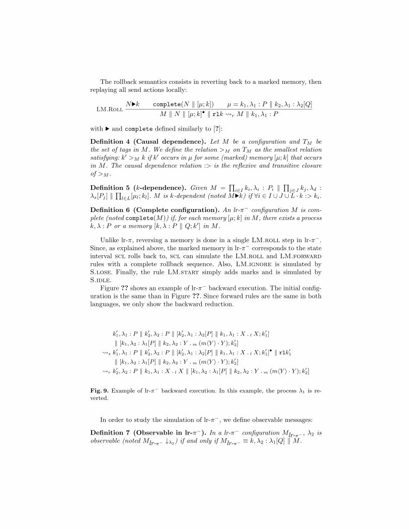
The rollback semantics consists in reverting back to a marked memory, thenreplaying all send actions locally:

LM.RollN·k complete(N || [µ; k]) µ = k1, λ1 : P || k2, λ1 : λ2[Q]

M || N || [µ; k]• || rlk r M || k1, λ1 : P

with · and complete defined similarly to [?]:

Definition 4 (Causal dependence). Let M be a configuration and TM bethe set of tags in M . We define the relation >M on TM as the smallest relationsatisfying: k′ >M k if k′ occurs in µ for some (marked) memory [µ; k] that occursin M . The causal dependence relation :> is the reflexive and transitive closureof >M .

Definition 5 (k-dependence). Given M =∏i∈I ki, λi : Pi ||

∏j∈J kj , λd :

λs[Pj ] ||∏l∈L[µl; kl]. M is k-dependent (noted M·k) if ∀i ∈ I ∪ J ∪L · k :> ki.

Definition 6 (Complete configuration). An lr-π− configuration M is com-plete (noted complete(M)) if, for each memory [µ; k] in M , there exists a processk, λ : P or a memory [k, λ : P || Q; k′] in M .

Unlike lr-π, reversing a memory is done in a single LM.roll step in lr-π−.Since, as explained above, the marked memory in lr-π− corresponds to the stateinterval scl rolls back to, scl can simulate the LM.roll and LM.forwardrules with a complete rollback sequence. Also, LM.ignore is simulated byS.lose. Finally, the rule LM.start simply adds marks and is simulated byS.idle.

Figure ?? shows an example of lr-π− backward execution. The initial config-uration is the same than in Figure ??. Since forward rules are the same in bothlanguages, we only show the backward reduction.

k′1, λ1 : P || k′2, λ2 : P || [k′2, λ1 : λ2[P ] || k1, λ1 : X .l X; k′1]

|| [k1, λ2 : λ1[P ] || k2, λ2 : Y .m (m〈Y 〉 · Y ); k′2]

s k′1, λ1 : P || k′2, λ2 : P || [k′2, λ1 : λ2[P ] || k1, λ1 : X .l X; k′1]• || rlk′1|| [k1, λ2 : λ1[P ] || k2, λ2 : Y .m (m〈Y 〉 · Y ); k′2]

r k′2, λ2 : P || k1, λ1 : X .l X || [k1, λ2 : λ1[P ] || k2, λ2 : Y .m (m〈Y 〉 · Y ); k′2]

Fig. 9. Example of lr-π− backward execution. In this example, the process λ1 is re-verted.

In order to study the simulation of lr-π−, we define observable messages:

Definition 7 (Observable in lr-π−). In a lr-π− configuration Mlr-π− , λ2 isobservable (noted Mlr-π− ↓λ2) if and only if Mlr-π− ≡ k, λ2 : λ1[Q] || M .

Notice that marked messages are not observable. We refine the definition ofobservable message in scl:

Definition 8 (Observable in scl (2)). In a scl configuration Mscl, d is ob-servable (noted Mscl ↓d) if and only if there exists a 〈k, ssn,AG, si,Q, inc〉 ∈ sLdand the incarnation number of k is inc.

This definition only differs from the first one in the way that only messageswhich have been sent since the last rollback are observable.

Theorem 3 (Simulation). The relation R = {(M,γ−1+ (M))|M ∈ Clr-π−} isa weak barbed simulation.

The proof is similar to the proof of Theorem ?? and is provided in [?].

5 Related Work

We do not know of any work that attempts to relate a distributed checkpointrollback scheme with a reversible model of computation, as we do in this paper.However, our work touches upon several topics, including the formal specificationand verification of distributed checkpoint rollback algorithms, the definition ofrollback and recovery primitives and abstractions in concurrent programminglanguages and models, and the study of reversible programming models andlanguages. We discuss these connections below.

Several works consider the correctness of distributed checkpoint rollback al-gorithms. The Manetho algorithm was introduced informally using pseudo codeand proved correct in [?,?]. Several other checkpointing algorithms have beenconsidered and proved correct, such as e.g. adaptive checkpointing [?] or check-pointing with mutable checkpoints [?]. Our proof of correctness for Manethorelies on a more formal presentation of the algorithm, by way of operationalsemantics rules, and the analysis of the associated transition relation. In thatrespect, the work which seems closer to ours is [?], which also formalizes acheckpointing algorithm (the algorithm from [?], which is not a causal loggingcheckpoint/rollback algorithm) by means of operational semantics rules, and alsoproves its correctness by an inductive analysis of its transition relation.

The rollback capability in lr-π is directly derived from the low-level semanticsof roll-π [?]. Compared to [?], the rollback capability in lr-π can be triggeredby the occurrence of a process crash, but we have shown above that this couldbe encoded in roll-π. Undo or rollback capabilities in programming languageshave a long history (see e.g. [?] for an early survey in sequential languages).More recent works which have introduced undo or rollback capabilities in aconcurrent programming language or model include [?], which defines loggingand group primitives for programming fault-tolerant systems, [?], which extendsthe actor model of computation with primitives for creating globally-consistentcheckpoints, [?], which introduces checkpointing primitives in concurrent ML,[?], which extends the Klaim tuple space programming language with rollbackcapabilities directly inspired by roll-π, and [?] which extends a subset of Core

Erlang with a reversible semantics similar to the roll-π one. The rollback ca-pabilities in roll-π have several advantages over these different works: rollbackis possible at any moment during execution, in contrast to [?]; does not sufferfrom the domino effect, in contrast to [?]; and provides direct support for con-sistently undoing all the consequences of a given action, in contrast to [?]. Thesame properties hold for lr-π and reversible Klaim.

6 Conclusion

We have shown in this paper the tight relationship that exists between a check-point/rollback scheme based on causal logging and a reversible concurrent pro-gramming model based on causal consistency. More precisely, we have shownthat the scl language, whose operational semantics formalizes the behaviour ofthe Manetho algorithm, can be (weakly barbed) simulated by lr-π, a reversibleasynchronous concurrent language with process crash failures, based on the roll-πlanguage, a reversible π-calculus with explicit rollbacks. The converse is not true,but we have shown that scl can (weakly barbed) simulate a variant of lr-π withlimited rollbacks. These results probably extend to other checkpoint/rollbackschemes based on causal logging, but one would need first to formally specifythem as we did in this paper for Manetho.

Apart from showing this relationship, the results are interesting for severalreasons. On the one hand, they point to interesting extensions to causal loggingcheckpoint/rollback schemes. In effect lr-π constitutes an extension of check-point/rollback causal logging that does not limit rollbacks to the last savedcheckpoint of a failed process: this can be a useful feature to protect againstcatastrophic faults such as those resulting from faulty upgrades. Also, it is triv-ial to add to lr-π the ability to create new processes and to exchange processes inmessages as in roll-π, thus extending checkpoint/rollback capabilities to dynamicenvironments, where new code can be added and new processes can be created atruntime, or to add compensation capabilities as in [?] to avoid retrying a faultyexecution path. We do not know of checkpoint/rollback schemes that combinethese different capabilities and the tight connection established in this papershows with lr-π how they can be added to causal logging checkpoint/rollbackschemes. On the other hand, they suggest interesting directions to optimize roll-back in reversible concurrent languages. For instance, as in Manetho, one canavoid rolling back all processes in lr-π by a judicious use of local replay.