Consistent tangent operators for rate-independent elastoplasticity

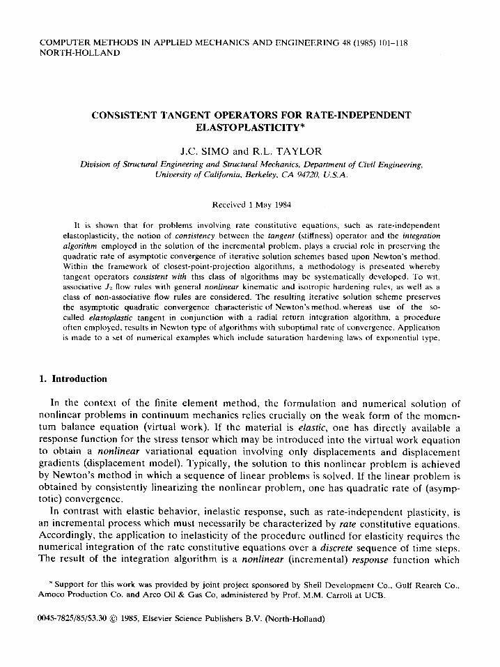
COMPUTER METHODS IN APPLIED MECHANICS AND ENGINEERING 4X (1985) 101-118

NORTH-HOLLAND

CONSISTENT TANGENT OPERATORS FOR RATE-INDEPENDENT ELASTOPLASTICITY”

J.C. SIMO and R.L. TAYLOR

Division of Structural Engineering and Structural Mechanics, Department of Civil Engineering,

University of California, Berkeley, CA 94720, U.S.A.

Received 1 May 1984

It is shown that for problems involving rate constitutive equations, such as rate-independent

elastoplasticity, the notion of consistency between the tangent (stiffness) operator and the integration

algorithm employed in the solution of the incremental problem, plays a crucial role in preserving the

quadratic rate of asymptotic convergence of iterative solution schemes based upon Newton’s method. Within the framework of closest-point-projection algorithms, a methodology is presented whereby tangent operators consistent with this class of algorithms may be systematically developed. To wit, associative JZ flow rules with general nonlinear kinematic and isotropic hardening rules, as well as a class of non-associative flow rules are considered. The resulting iterative solution scheme preserves the asymptotic quadratic convergence characteristic of Newton’s method, whereas use of the so- called elastoplastic tangent in conjunction with a radial return integration algorithm, a procedure often employed, results in Newton type of algorithms with suboptimal rate of convergence. Application is made to a set of numerical examples which include saturation hardening laws of exponential type.

1. Introduction

In the context of the finite element method, the formulation and numerical solution of nonlinear problems in continuum mechanics relies crucially on the weak form of the momentum balance equation (virtual work). If the material is elastic, one has directly available a response function for the stress tensor which may be introduced into the virtual work equation to obtain a nonlinear variational equation involving only displacements and displacement gradients (displacement model). Typically, the solution to this nonlinear problem is achieved by Newton’s method in which a sequence of linear problems is solved. If the linear problem is obtained by consistently linearizing the nonlinear problem, one has quadratic rate of (asymptotic) convergence.

In contrast with elastic behavior, inelastic response, such as rate-independent plasticity, is an incremental process which must necessarily be characterized by rate constitutive equations. Accordingly, the application to inelasticity of the procedure outlined for elasticity requires the numerical integration of the rate constitutive equations over a discrete sequence of time steps. The result of the integration algorithm is a nonlinear (incremental) response function which

* Support for this work was provided by joint project sponsored by Shell Development Co., Gulf Rearch Co., Amoco Production Co. and Arco Oil & Gas Co, administered by Prof. M.M. Carroll at UCB.

00457825/85/$3.30 @ 1985, Elsevier Science Publishers B.V. (North-Holland)

102 J.C. Simo, R.L. Taylor, Tangent operators for elastoplasticity

defines the stress tensor as a function of the strain history up to the current time step. Thus, the integration algorithm enables one to formally treat the elastoplastic problem over a typical time step as an equivalent elastic problem. The crucial point we wish to emphasize is that the tangent moduli that appear in the linearized problem must be obtained by consistent linearization of the response function resulting from the integration algorithm, in order to preserve the quadratic rate of asymptotic convergence. A complete account of consistent linearization procedures relevant to nonlinear continuum mechanics can be found in [8, chapter 41.

For rate-independent plasticity the so-called return mapping algorithms provide an effective and robust integration scheme of the rate constitutive equations. This procedure amounts to a ‘discrete’ enforcement of the consistency condition and appears to have been suggested first by Wilkins [16]. Geometrically, the return mapping algorithm amounts to finding the closest distance of a point to a (cowex) set. Within the framework of this class of algorithms we present a systematic procedure whereby for rate-independent plasticity with arbitrary (nonlinear) laws of isotropic and kinematic hardening, an explicit expression for the tangent moduli consistent with the integration algorithm is derived. We note that radial return algorithms have been often employed in conjunction with the so-called elustoplustic tangent [3, 141. These elastoplastic moduli are obtained from the ‘continuum’ rate constitutive model by enforcement of the consistency condition. Such a procedure, however, results in loss of the quadratic rate of asymptotic convergence particularly important for large time steps. This fact was recognized by Nagtegaal [lo] in the context of a linear isotropic hardening rule.

In addition to classical plasticity models, although with arbitrary (nonlinear) hardening laws, we also consider an example of non-associative plasticity of interest in the modeling of geological materials. The ideas presented herein are illustrated through a set of numerical

examples.

2. Associative J2 plasticity: Nonlinear hardening rules

In this section we consider the formulation of the basic equations of our model problem for associative plasticity. Emphasis is placed on the numerical characterization of plasticity and thus attention is restricted to linear isotropic elastic behavior. The model includes nonlinear isotropic and kinematic hardening rules which are specified by a hardening parameter and a plastic modulus for the back stress. These parameters are assumed to be arbitrary functions of the ‘equivalent’ plastic strain. Classical linear isotropic and kinematic hardening (e.g. the Prager-Ziegler rule) as well as saturation type of hardening rules such as that proposed by Vote [15], are included in the model discussed.

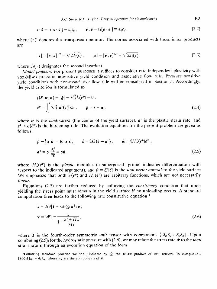
The following notation will be employed. We denote by s and e the deviatoric stress and strain tensors, so that

s = u - +(tr a)1 , e = E - f(tr e)l , W)

where 1 is the second order unit tensor and tr( * ) designates the truce operator. The linear vector spaces of deviutoric stress and deviutoric strain tensors will be equipped with the natural (Euclidean) inner product induced by the trace of the product of two tensors; that is,

J.C. Sirno. R.L. Taylor. Tangent operators for elastoplasticit) 103

S 1 i = tr[s ’ St] e SijSji , e : 2 = tr[e - 2’1 z f?,E~j, (2.2)

where (- )’ denotes the transposed operator. The norms associated with these inner products

are

llsll = [s : s] I’* = ~2J*(s) , JlelJ = [e : e]“’ = m, (2.3)

where J2( .) designates the second invariant. Model problem. For present purposes it suffices to consider rate-independent plasticity with

von-Mises pressure insensitive yield condition and associative flow rule. Pressure sensitive

yield conditions with non-associative flow rule will be considered in Section 5. Accordingly, the yield criterion is formulated as

g=s-ff, (2.4)

where (Y is the back-stress (the center of the yield surface), dP is the plastic strain rate, and dp+ K(f?“) is the hardening rule. The evolution equations for the present problem are given as follows:

S = 2G(i - dP), ci = fHp$fP )

(2.5)

where HA(kp) is the plastic modulus (a superposed ‘prime’ indicates differentiation with respect to the indicated argument), and ri = &I[~/[ ’ 1s t h e unit vector normal to the yield surface We emphasize that both K(cP) and H,(Zp) are arbitrary functions, which are not necessarily

linear. Equations (2.5) are further reduced by enforcing the consistency condition that upon

yielding the stress point must remain in the yield surface if no unloading occurs. A standard computation then leads to the following rate constitutive equation:’

S=2G[I-yri@ri]:8,

y = IJdPIJ = 1

K’f HA’

‘+ 3G

(2.6)

where I is the fourth-order symmetric unit tensor with components +{8ik8j/ + Si,Sj,}. Upon combining (2.9, for the hydrostatic pressure with (2.6), we may relate the stress rate Cr to the total strain rate 6 through an evolution equation of the form

‘Following standard practice we shall indicate by @ the tensor product of two tensors. In components [a@ ri]ij*/ = riijrikr, where nij are the components of ri.


(2.7a)

where ceP(a) is a fourth-order tensor, often referred to as the elustoplastic (tangent) moduli, which has the explicit expression

ceP(a) = Kl@ 1+ 2G[I - fl @I l] - 2Gyri @ ri . (2.7b)

We shall refer to.(2.7b) as the continuum elastoplastic tangent operator in order to make the distinction, crucial to the development that follows, with its discrete version to be derived in Section 4.

3. Integration scheme: Return mapping algorithm

From a computational standpoint the elastoplastic problem may be treated as a strain controlled problem in the sense that the stress history is obtained from the strain history by means of an integration algorithm. An effective procedure for numerically integrating the elastoplastic problem is to employ the so-called return mapping algorithms. The basic idea is illustrated in Fig. 1 for the case of pressure insensitive perfect plasticity. From the converged solution at time t = t,,

one computes an elastic trial stress s:+~. If the resulting state defined by ST+, lies outside of the elastic region enclosed by the yield surface Z’, one defines the final state as the closest-point- projection of sz+i onto the yield surface. Thus, we have the two-step algorithm

sz+1= s, + 2GAe,+, , s,+l= I-%:+1). (3.1)

where P : W5+ JC denotes the (orthogonal) projection onto the elastic region C, a compact set with boundary JC (the yield surface). From a geometric standpoint this procedures amounts to enforcing the consistency condition at the end of each time step and appears to have been first proposed by Wilkins [16]. Error analyses for several return schemes have been considered in detail by Krieg and Krieg [6], and by Schreyer, Kulak and Kramer [13]. For a recent survey discussion see [4]. From a mathematical standpoint it can be shown that closest-point-

Fig. 1. Return mapping algorithm. Perfect plasticity.

J.C. Sitno, R.L. Taylor. Tangent operators for elastoplasticity 10s

projection algorithms defined a contraction mapping in a suitable Hilbert space, and thus produce unconditionally stable algorithms [12].

For an arbitrary convex yield function, the numerical integration of the elastoplastic problem is thus reduced to the standard minimization problem of finding the minimum distance of a point to a convex set. In the particular case of the von-Mises yield condition with associative flow rule and isotropic hardening, the closest-point-projection is trivially defined and leads to the so-called radial return algorithm. The superiority of this procedure over several other proposed projection schemes is now well established [4, 131. In what follows we summarize the

basic integration scheme, modified to account for kinematic hardening, essentially as presented in [5]. It should be noted, however, that since this work is in the context of explicit algorithms, no reference to the need of tangent operators is made.

Radial return algorithm. Nonlinear isotropic and kinematic hardening. Let ri denote the unit vector field normal to the yield surface at the end of a typical time step [t,, I”+~]. We then have

(3.2)

where tn+i = s,+~ - (Y,+]. The stress s~+~ at the end of the step is then computed from the trial elastic stress ST+, according to

T Sri+++ = Sri+++ - yAt2Gii, T

Sn+l = s, + 2GAe,+, . (3.3)

To enforce the consistency condition at t,,, it is necessary to define the yield surface at the end of the time step and hence to determine the hardening parameter and back-stress at t,,+,.

These variables depend in turn on the equivalent plastic strain which, upon evaluating (2.4), with the mid-point rule, becomes

I tn+ 1

-P en+, = tF;+ d/%[ld”(r)/l dr = gp,+ V$[ yht] . (3.4) r”

The evolution equation (2.5)3 may now be integrated to obtain, with the aid of (3.4), the result

a,+1 = a,, + :H;(Z:+&yAt]fi

= (Y, + fl[H,(d;+,)- &(e:)]ri. (3.5)

Introducing the notation AH, = H,(2P,+1)- H,(EP,), from (3.3) and (3.5) we obtain

Sn+* = s,+~ - (Y,+~ = gel - [~GYA~ + flh~,]ii, (3.6)

where &z = s;f+, - LY,+~. Since by (3.2) we have tn+r = ]]tn+l]]ri, it follows from (3.6) that the unit normal n^ is determined in terms of the trial elastic stress lx+, according to

(3.7)

106 J.C. Simo, R.L. Taylor, Tangen? operators for elastoplashcity

From (3.6) and (3.7) it then follows that the enforcement of the consistency condition reduces to the scalar equation

g(yAt) = - +(e:+,)+ jI&f+,lj - [2GrAt + ti:AH,] = 0. (3.8)

Since fZz+l = C?, + d:rAt, for prescribed functions ~(2”) and II, (3.8) yields an equation (generally nonlinear) from which the value of [y At] is determined. The solution of (3.8) may be effectively accomplished by the simple local Newton iteration procedure summarized in Table 1.

For convenience, a step-by-step description of the algorithm discussed in this section has been summarized in Table 2. We notice that for linear isotropic and kinematic hardening rules it reduces to that proposed by Krieg and Key [5]. The same algorithm restricted to linear isotropic hardening also has been employed by Nagtegaal [lo]. The geometric interpretation of the algorithm is contained in Fig. 2.

REMARK 3.1. Variables at time t = tn+l in Table 2, (. ) “+I, to the ith iteration within the time step [tn, t,+l]; i.e., ( s)i,+l.

are understood to correspond

REMARK3.2. Notice that according to the algorithm in Table 1 the values ( -)i+I are calculated

based solely on the converged values (* ),, at the beginning of the time step t = t,,. The (nonconverged) values ( .)L;1I at the previous iteration play no explicit role in this stress

calculation

Table 2 Radial return algorithm. Nonlinear kinematic/isotropic hardening

Table 1 Consistency condition: determination of [rAtI

(i) ~~‘:l= ~pn(:;‘) + ~/25A(k)

I H;+K’ (*)

(ii) Dg(,+“‘) = -2G 1 + ___ 3G 1

(iii) A g(h’k’) (k+l)= ~‘k’___-_--

Dg(A (k’)

(iv) If \g(A’“‘)I > TOL then k + k + 1 and go to (i)

6)

(ii)

(iii)

Compute trial elastic stress,

S:+I = sn + 2GAe,+l,

g+, = ST+, - ff”

Compute unit normal field ri,

Find [yht] by local iteration, Table 1. Compute

the equivalent plastic strain at f,,+l,

(iv) Compute back-stress and deviatoric stress,

a,+1 = an + x~AH._(z+~)~~,

Sn+t = a,+1 + V/3K(k:+l)a

(v) Add elastic volume change

un+l = sn+] + K tr AE~

J.C. Simo, R.L. Taylor, Tangent operators for elastoplasticity 107

Fig. 2. Nonlinear kinematic hardening. Radial return algorithm.

REMARK 3.3. If the elastic trial stress s Ti+l at the ith iteration were computed from the

nonconverged stresses s L-:1 at the previous iteration (rather than from converged stress s, as in Table 2) then the ‘continuum’ elastoplastic tangent (2.7b) becomes the consistent tangent for this particular algorithm. However, use of an iteration scheme based on intermediate nonconverged values appears to be questionable for a problem which, physically, is ‘path-dependent’. In addition, if ‘unloading’ within the iteration process occurs, a new iteration starting from the converged stresses s, is necessary.

4. Variational problem: Consistent tangent operator

In this section we shall develop the tangent operator consistent with the algorithm summarized in Table 2 above. The crucial point is to realize that we no longer have a ‘continuum’ problem described by constitutive equations (2.5). Since we may assume that

( a,, a”,, E,) are known at a time t = t,,, as a result of the radial return algorithm in Table 2, we now have a nonlinear ‘incremental’ model governed by constitutive equations

AC = E - E, + &((a,, e”,, E,, E - E”) . (4.1)

Given an increment of strain AE we compute a uniquely defined stress through the radial return algorithm symbolically given by the mapping (4.1). Although (4.1) is asymptotically consistent with the elastoplastic model (2.5) the distinction between both models is essential.

In addition to (4.1) we have the momentum balance equation, the weak form of which (virtual work) may be formulated as follows. Let b(x) the body force and further let t(x) be the traction vector specified on the part &R of the boundary ati. Let U(X) be specified on &R as uJad = ii, where we require that &fl n cY,R = 0 and a,R U d,R = X2. For specified initial data at t = t,, the momentum balance equation reads

(4.2)


for any admissible variation r/ E H’(R) such that q lavR = 0. Since the treatment of the transient dynamic problem plays no role in the development of the consistent tangent operator that follows, we shall ignore inertia effects and confine our attention to the static case.

The solution of problem (4.1)-(4.2) within the context of the finite element method is accomplished by an iterative scheme based on Newton’s method. Accordingly, one solves a sequence of (consistently) linearized problems given by

DG(u:+l, ~)a Au:,, = I

Vq : [&+I :V(Au;+l)] do = -G(u;+l, q), (4.3) R

until the residual G(u~,+~, r)) vanishes (to within a prescribed tolerance). In (4.3) subscripts refer to the time step and superscripts to iteration within the time step. We now come to the essential point of our discussion: the derivation of an expression for the ‘tangent moduli’ c;+~ consistent with the radial return algorithm summarized in Table 2.

Consistent tangent operator. From steps (iv) and (v) in Table 2 the incremental response function a(~“, E,, a:, E - E,) in (4.1) has the following explicit form:

&(a”, E,,, C”,, E - E,) = K(tr A l n+Jl + (Y,+~ + R,+lri, (4.4)

where R,+l = d\/3K(~;+1) is the radius of the yield surface at t = tn+l. The tangent moduli

cn+, in (4.3) is then defined as

d6(U”, E”, a:, E - E”) C n+1=

de (4.5)

E=C”+,

In what follows explicit indication of the arguments in 6 as well as superscripts referring to iteration will be omitted. In order to carry out the computation of (4.5) use will be made of the following result.

LEMMA 4.1. The derivative of the unit normal field ri (5) = &//j&11 is given by the formula

(4.6)

PROOF. The result easily follows with the aid of the directional derivative. First we note that for an arbitrary vector h E Iw6 we have

By the chain rule it then follows that

&+ah)

so that (4.6) holds. 0

1 :h


In addition we recall the following two formulae which result from a straightforward application of the chain rule:

(4.7)

Thus, with the aid (4.6) and (4.7) we obtain from (4.4) and (4.5) the following expression for c,+,:

c,+,=K1@1+2G &[‘&1@1]-2G$7@fi n+l n+l

+iig) al?,+, da,+1 -+- ae II+1 de . II+1

(4.8)

Next, we note that the last two terms in (4.8) may be explicitly computed from the algorithm as follows.

(a) Computation of h @ dR n+liaEn+l. Taking derivatives with respect to l n+1 of the scalar consistency condition (3.8) we may solve for Atdy/ae,+l to obtain

aY 1 At-= ri.

ae [K’+ El,+1 (4.9)

?I+1 1+ 3G

Hence, since R,,, = VjK(c?“,+,), taking the derivative with respect to E”+~, noting that -P

e,+l = Z: + fly At and using (4.9) we obtain the expression

aRn+, 2 K:+I [email protected]

aE 31+’ iigii.

n+l K’f H&+1 3G

(4.10)

(b) Computation of dcx,,+l/den+l. Since (Y,+~ is explicitly given by step (iv) in Table 2, taking derivative with respect to E n+l and using (4.6) together with (4.9) we arrive at

n+l=p AHa aff ac nil

3m[I-j1@1- li@ii]+:N:,+lhtir@- n+l de nil

ii@li. (4.11)

3G

By substitution of (4.10) and (4.11) into (4.8) we obtain the final expression for the ‘tangent moduli’ consistent with the radial return algorithm for nonlinear isotropic/kinematic hardening summarized in Table 2.

c,+,=K1~1+2G~[1-~1~1]-2Gj+i@ri, (4.12)


where p and 7 are given by

3G

(4.13)

REMARK 4.2. (i) Expression (4.12) should be compared with (2.7b) for the ‘continuum’ elastoplastic tangent. We observe that as a result of the radial return algorithm the shear modulus G enters in the ‘consistent’ tangent (4.12) scaled down by a factor /3 defined by (4.13),. In addition, the factor 2Gy appearing in (2.7b), is replaced in (4.12) by 2Gy, where 7 is defined by (4.13)*.

(ii) Notice that p s 1, and that for large time steps s z+1 may lay far out of the yield surface so that p may become significantly less than unity. In addition, since 7 = y + p - 1, where y is defined by (2.6) 2, we have the bound y - 1~ 7 d y. Therefore, for large time steps, the consistent tangent moduli (4.12) may differ significantly from the ‘continuum’ elastoplastic tangent (2.7b).

(iii) As a result of (ii) use of the ‘continuum’ elastoplastic tangent (2.7b) in conjunction with the radial return algorithm summarized in Table 2 leads to loss of the quadratic rate of asymptotic convergence which characterizes Newton’s method.

5. Non-associative plastic flow: An example

In this section we show that the procedure discussed above in the context of classical J2 associative plasticity applies equally to nonclassical models with a non-associative flow rule. Again wt: wish to emphasize that once an algorithm has been employed to numerically integrate a given rate constitutive equation, the tangent moduli which appear naturally in the formulation of the linearized incremental problem (in the present context nonsymmetric) must be derived from the integrated constitutive equation; the original rate constitutive equation no longer plays a role.

Non-associative model problem. As in Section 2 we shall assume isotropy for the elastic part of the model. However, instead of the yield criterion (2.4) we now consider a pressure sensitive yield condition of the form

f(S, p) = [ISI - q/3K(p) = 0, p = f tr u . (5.1)

We confine ourselves to the case in which the flow rule is pressure insensitive, and consider the simplest case in which the flow potential is of the form g(a) = (Is/I. Thus, the flow rule is then given as in the associative case by

(5.2)

REMARK 5.1. Well-known pressure sensitive yield criterions (e.g. Drucker-Prager) are characterized by equations of the form (5.1).


Fig. 3. Saturation type of yield condition. f(s, p) = j(sjl- [cm - (c- - CO) exp(-p/T)].

REMARK 5.2. The choice of an exponential form for the pressure-dependent function K(p) in (5.1) leads to a saturation type of yield condition illustrated in Fig. 3, which together with the flow rule (5.2) produces a simple non-associative rate-independent plasticity model of some interest in the modeling of the behavior of some geological materials. The reason for this is that the flow rule (5.2) tends to correct the often excessive dilatancy predicted by the normality rule in conjunction with, say, Drucker-Prager yield condition.

In addition to (5.1) and (5.2) we have the evolution equation

S = 2G(t - d”) , (5.3)

which completes the formulation of the model. Enforcement of the consistency condition ieads to the following expression for the (nonsymmetric) elastoplastic tangent:

ceP(u)=[K-~G]1~l+2G[I-R@R]+KV$~‘(p)R~l, (5.4)

so that (5.3) may be written as s’ = ceP(u): ti. Return mapping algorithm. Because of the particular form (5.2) of the flow rule chosen, the

return mapping algorithm takes an extremely simple form. The key observation is that if the trial elastic stress sT lies outside of the yield surface, the projection onto the yield surface consistent with the flow rule (5.2) must leave the elastic trial hydrostatic pressure unchanged. This idea is illustrated geometrically in Fig. 3. Accordingly, one first computes the elastic trial stress in the standard manner as

p:+1= pn +KtrAe,+l, T Sn+1 = s, + 2GAe,+, . (5.5)

If the trial state is outside of the yield surface; i.e., f(~:+~, P:+~)> 0, then the closest-point- projection onto the yield surface consistent with (5.2), is given simply by

p,+1 T

= pn+1,

S n+l = d$K(p,+~)ri , ii = S;+I/((~+I(\ . (5.6)


Equations (5.5) and (5.6) define a nonlinear incremental constitutive equation of the form (4.1). The tangent moduli consistent with this model, thus asymptotically consistent with (5.4) are defined by (4.5) and may be obtained as follows.

Consistent tangent moduli. Making use of Lemma 4.1 in conjunction with formulae (4.7) we obtain the following expression for the tangent moduli cn+] = d~~+~/&~+~:

C n+l = Kl@ l+ 2Gp[I+l@ l]-2G@@ ri +K~~~~(p,+~)ri@l, (5.7)

(5.8)

Comparison of (5.7) with expression (5.4) for the elastoplastic tangent shows that as a result of the return mapping algorithm the shear modulus G appears scaled down in the consistent tangent (5.7) by the factor p defined in (5.8). Since for large time steps one expects p to become significantly less than unity, use of the elastoplastic tangent defined by (5.4) in the solution of the linearized problem (4.3) would result in loss the quadratic rate of asymptotic convergence.

6. Numerical examples

In this section we present three examples that illustrate the practical importance of consistent tangent operators in a Newton solution procedure. Our objective is to exhibit the significant loss in rate of convergence that occurs when the elastoplastic ‘continuum’ tangent is used in place of the tangent consistently derived from the integration algorithm. In all the examples we use a 4-node bilinear isoparametric quadrilateral element combined with a constant pressure field. Accordingly, our approach is analogous to a mixed formulation typically employed in the treatment of the incompressibility constraint (e.g., see [19]). In the context of plasticity, the importance of an appropriate treatment of the pressure field was first recognized by Nagtegaal, Parks and Rice [ll]. Although the 4-node bilinear element with constant pressure interpolation does not strictly satisfy the LBB condition (e.g., see [l, Section 3.2]), a sufficient condition for convergence in the encompressible regimen, it performs satisfactorily in practical situations (e.g., see [lo]). Indeed this element forms the basis for many widely used computer programs (e.g., [2]).

Our global solution algorithm may be summarized as follows. After elimination of the pressure field at the element level, the discrete version of the variational equation (4.3) may be written for each iteration, i, within the time [t,,, t,+,] as

K,(a;+&hzi,+~ = R(u;+I), (6.1)

where a,!, represents the vector of nodal displacement, and KT(ak+l), R(u’,+~) are the tangent stiffness matrix and the residual force vector at the configuration defined by ~f+~. The nodal displacement vector is updated according to

i+l _ i a,+1 - a,+1 + Au’,+* (6.2)


Convergence of the discrete problem is measured in terms of the (discrete) energy norm, which is computed from the residual and incremental displacement vectors as

AE(a;+i) = {Aa?:1)‘R(a’,+l) . (6.3)

Alternative discrete norms may be used in place of (6.3) in particular the Euclidean norm of the residual force vector. In the numerical examples described below we shall often display the behavior of this norm for comparison purposes. In terms of the energy norm (6.3) our termination criteria for the Newton solution strategy takes the following form:

AE(a;+,) d 10-9AE(at,+1). (6.4)

While this appears to be a very severe condition to achieve, it will be shown through the numerical examples that condition (6.4) is easily attained when a consistently derived tangent operator is used.

EXAMPLE 6.1. Thick-walled cylinder under internalpressure. As our first example we consider an infinitely long thick-walled cylinder subjected to internal pressure loading. The inner and outer radii of the cylinder are 5 m and 15 m, respectively. The properties of the material are chosen as E = 70 MPa, v = 0.2. In addition, we consider isotropic and kinematic hardening rules of the exponential type, defined according to the expression

8~(tT~)+(1-8)&= Y,-[Y,- Yo]ey"'+ %Zp, ~E[O, 11. (6.5)

We note that 6 = 0 and 6 = 1 correspond to the limiting cases of pure kinematic and pure isotropic hardening rules, respectively. The values for the parameters in (6.5) are taken as

Y0=0.243MPa, Y,=0.343MPa, y=O.lMPa, Y=O.l5MPa, S=O.l.

(6.6)

The body is assumed to be undisturbed at time zero, and the internal pressure is increased linearly in time until the entire cylinder yields. The finite element mesh employed in the calculation is shown in Fig. 4(a). The size of the time step was selected as to achieve yielding of the entire transverse section in two time steps involving plastic deformation. The position of the elastic-plastic interface in these two time steps is depicted in Fig. 4(b). The calculation was performed with both the ‘continuum’ and the ‘consistent’ elastoplastic tangent, and the results are displayed in Table 3. Notice that in spite of the better performance exhibited by the

I -

I I Im -

I I STEb 1 STE-P 2

Fig. 4(a). Thick-wall cylinder. Finite element mesh. Fig. 4(b). Thick-wall cylinder. Elastic-plastic interface.


Table 3

Number of iterations for each time step

Step 12 345

State el el-el el-pl pl pl Continuum 2 6 9 10 6

Consistent 25 753

‘consistent’ tangent, one does not obtain a substantial reduction in the required number of iterations for convergence except in the fully plastic situation. This is due to the simplic- ity and well-posedness of the boundary value problem at hand; essentially one-dimen- sional. The next example will confirm this observation. We finally note that for the nonlinear yield condition (6.5) convergence with the local algorithm described in Section 4 and summarized in Table 1, was attained in 3-4 iterations. The effectiveness of this procedure is thus demonstrated.

EXAMPLE 6.2. Perforated strip under uniaxial extension. As our second example we consider the plane strain problem of an infinitely long rectangular strip with a circular hole in its axial direction, subjected to increasing extension in a direction perpendicular to the axis of the strip and parallel to one of its sides. The elastic properties of the material are taken as E = 70 MPa, v = 0.2, and the parameters in the saturation type of hardening rule (6.5) are assumed to be Y, = 0.243 MPa, Y,, = Y,, Y = 0, and S = 1. Thus, in this example we assume perfectly plastic behavior. Loading is performed by controlling the vertical displacement of the top and bottom boundaries of the rectangular strip. The finite element mesh employed is shown in Fig. 5 For obvious symmetry reasons, only t of the strip needs to be considered. The evolution of the elastic-plastic interface with increased straining of the strip is shown in Fig. 6. For the purpose

:

I8 m

/ n

Fig. 5. Perforated strip. Finite element mesh. Fig. 6. Perforated strip. Elastic-plastic interface.


of plotting these results, the stresses computed at the Gauss points of a typical element are projected onto the nodal points by means of bilinear interpolation functions. Related ‘smoothing’ procedures are discussed in [17, Section 11.51 and references therein, and are often used as a device for filtering spurious pressure modes (e.g., [7]).

The calculation was performed with both the ‘continuum’ and the ‘consistent’ tangent operators, and the number of iteration required to attain convergence is summarized in Table 4. The numerical values of the energy norm in a typical iteration are displayed in Table 5 and the values of the Euclidean norm of the residual for the same iteration in Table 6. The vastly superior performance of the ‘consistent’ tangent is apparent from these results. One should also note that the Euclidean norm of the residual lags behind the energy norm in the iteration process. This norm gives a direct measure of how well the momentum balance condition is satisfied. With the ‘consistent’ tangent operator, convergence in the energy norm is also accompanied by convergence in the Euclidean norm of the residual. However, from Table 5 and Table 6 we observe that convergence in the energy norm to within the tolerance prescribed in (6.4) does not imply convergence to within the same tolerance in the Euclidean norm of the residual, if the ‘continuum’ tangent is employed. Thus, an even more dramatic comparison in performance could have been drawn had we employed the Euclidean norm of the residual in the termination criteria (6.4).

Table 4

Number of iterations for each time step

Step 12 34 5

State el el-pl el-pi el-pl el-pl

Continuum 2 13 23 23 22 Consistent 25 54 5

Table 5 Energy norm values for step 4

Iteration 1 2 3 4 5 6

Continuum Consistent

Iteration


0.14e + 2 0.80e - 2 0.61e - 3 0.18e - 3 0.89e - 4 0.47e - 7 O.l4e+ 2 O.lle- 1 0.77e - 4 O.lOe- 9

7 8 9 10 11 12

0.27e - 4 0.16e - 4 0.97e - 5 0.59e - 5 0.36e - 5 0.22e - 5 - -

Iteration 13 14 1.5 16 17 18 Continuum 0.13e - 5 0.85e - 6 0.52e - 6 0.32e - 6 0.20e - 6 0.12e - 6 Consistent - - - -

Iteration 19 20 21 22 23 Continuum 0.77e - 7 0.47e - 7 0.29e - 7 0.18e - 7 O.lle- 7 Consistent - - - -


Table 6 Residual norm values for step 4

Iteration 1 2 3 4 5 6


Iteration


Iteration Continuum

Consistent

Iteration Continuum Consistent

0.25e + 3

0.25e + 3

7

0.41e + 0

13

0.98e - 1

19 0.23e - 1

-

0.74e + 1 0.22e + 1 O.lle + 1 0.75e + 0 0.55e + 0

0.74e + 1 0.84e + 1 0.66e - 3 0.35e - 8

8 9 10 11 12

0.32e + 0 0.25e + 0 0.20e + 0 0.15e + 0 0.12e + 0 - - - - -

14 15 16 17 18

0.78e - 1 0.61e - 1 0.48e - 1 0.3%~ - 1 0.30e - 1 - - - - -

20 21 22 23

O.l8e- 1 O.l4e- 1 O.lle- 1 0.91e-2 - -

We also note that the example at hand provides a severe test for the global performance of the Newton solution strategy. The calculations reported here were performed with a time step of At = 0.0125 for the properties Indicated above. For twice this value of the time step the iteration procedure diverges. However, when the Newton solution procedure was combined with a line search procedure, as described in [9], global convergence was attained for a step size At = 0.1.

EXAMPLE 6.3. Thick hollow sphere. As our final example we consider a thick hollow sphere with its outer surface subjected to hydrostatic extension and its inner surface stress free. The elastic properties of the material are taken as E = 22700 MPa, v = 0.3333. In addition, we assume non-associative elastic-plastic behavior governed by the model described in Section 5, with a Drucker-Prager yield condition. Thus, the pressure dependent function K(P) in (5.1) takes the following explicit form

K(P) = c - tan $p, c = 2.70 MPa, tan 4 = 0.879 . (6.7)

The mesh employed in the finite element calculation is shown in Fig. 7. We note that the symmetry of the problem allows an exact solution which may be used to test the algorithm for the non-associative case discussed in Section 5. This is done in Fig. 8, where the analytical and finite element solutions for confining pressure field are plotted versus the porosity. It is interesting to note that the numerical solution was found to be relatively insensitive to the size of the time step but sensitive to the spatial discretization. In the calculation summarized in Table 7, yielding of the entire section is achieved only in two time steps. Essentially the same results are obtained with f of this time step. However, a relatively fine mesh is required to achieve acceptable accuracy, as displayed in Fig. 8. The reasons for this are not yet clear.

The required number of iterations to attain convergence with both the ‘continuum’ and the ‘consistent’ tangent operators is summarized in Table 7. Since convergence with the ‘continuum’ tangent was not achieved in the first time step after thirty iterations, no further calculation with this tangent was performed.


k-- 12.36 m 4

0 I I I I .2 .21 .22 .23 .24 .25 .26

phi (Porosity)

Fig. 7. Thick hollow sphere. Finite element mesh. Fig. 8. Thick hollow sphere: Non-associative Drucker-

Prager flow rule.

Table 7 Number of iterations for each time step

Step 1 2 3 4

State el-pl el-pl pl pl

Continuum >30 ? ? ?

Consistent 8 6 4 3

Acknowledgment

We wish to thank Dr. G.L. Goudreau and Dr. J.O. Hallquist at LLNL, and Prof. T.J.R. Hughes at Stanford U. for their encouragement and helpful discussions.

References

ill

PI

t31

141

151

G.F. Carey and J.T. Oden, Finite Elements, A Second Course, Vol. 11 (Prentice-Hall, Englewood Cliffs, NJ,

1983). G.L. Goudreau and J.O. Hallquist, Recent developments in large-scale finite element Lagrangian hydrocode technology, Comput. Meths. Appl. Mech. Engrg. 33 (1982) 725-757.

E. Hinton and D.R.J. Owen, Finite Elements in Plasticity: Theory and Practice, (Pineridge Press, Swansea,

Wales, 1980). T.J.R. Hughes, Numerical implementation of constitutive models: Rate-independent deviatoric plasticity, Workshop on Theoretical Foundations for Large Scale Computations of Nonlinear Material Behavior, Northwestern University, Evanston, IL (1983). R.D. Krieg and S.W. Key, Implementation of a time dependent plasticity theory into structural computer programs, in: J.A. Stricklin and K.J. Saczalski, eds., Constitutive Equations in Viscoplasticity: Computational

and Engineering Aspects, AMD-20 (ASME, New York, 1976).


[6] R.D. Krieg and D.B. Krieg, Accuracies of numerical solution methods for the elastic-perfectly plastic model, J. Pressure Vessel Technology, ASME 99 (1977) 510-515.

[7] R.L. Lee, P.M. Gresho and R.L. Sani, Smoothing techniques for certain primitive variable solutions of the Navier-Stokes equations, Internat. J. Numer. Meths. Engrg. 14(12) (1979) 1785-1804.

[8] J.E. Marsden and T.J.R. Hughes, Mathematical Foundations of EIasticity (Prentice-Hall, Englewood Cliffs, NJ, 1983).

[9] H. Matthies and G. Strang, The solution of nonlinear finite element equations, Internat. J. Numer. Meths. Engrg. 14 (1979) 1613-1626.

[lo] J.C. Nagtegaal, On the implementation of inelastic constitutive equations with special reference to large

deformation problems, Comput. Meths. Appl. Mech. Engrg. 33 (1982) 469-484. [ll] J.C. Nagtegaal, D.M. Parks and J.R. Rice, On numerically accurate finite element solutions in the fully plastic

range, Comput. Meths. Appl. Mech. Engrg. 4 (1974) 1.53-178.

[12] M. Ortiz, Topics in constitutive theory for nonlinear solids, Ph.D. Dissertation, Dept. of Civil Engineering, University of California, Berkeley, 1981.

[13] H.L. Schreyer, R.L. Kulak and J.M. Kramer, Accurate numerical solutions for elastic-plastic models, J. Pressure Vessel Technology, ASME 101 (1979) 226-234.

[14] P.M. Pinsky, KS. Pister and R.L. Taylor, Formulation and numerical integration of elastoplastic and elasto-viscoplastic rate constitutive equations, Rept. No. UCB/SESM-81/05 Dept. Civil Engrg. Univ. Califor-

nia, Berkeley, 1981.

[15] E. Vote, Metalurgia 51 (1955) 219. [16] M.L. Wilkins, Calculation of elastic-plastic flow, Methods of Computational Physics, 3 (Academic Press, New

York, 1964).

[17] O.C. Zienkiewicz, The Finite Element Method, (McGraw-Hill, Berkshire, England, 1977). [18] O.C. Zienkiewicz, R.L. Taylor and J.M.W. Baynham, Mixed and irreducible formulations in finite element

analysis, in: S.N. Atluri, R.H. Gallager and O.C. Zienkiewicz, eds., Hybrid and Mixed Finite Element Methods (Wiley, New York, 1983).

[19] R.L. Yaylor and O.C. Zienkiewicz, Mixed finite element solution of fluid flow problems, in: R.H. Gallagher, D.H. Norrie, J.T. Oden and O.C. Zienkiewicz, eds., Finite Elements in Fluids, Vol. 4 (Wiley, New York, 1982).

Consistent tangent operators for rate-independent elastoplasticity

Documents

Transcript of Consistent tangent operators for rate-independent elastoplasticity