Triple Tangent Flank Milling of Ruled

Surfaces

Cornelia Menzel1, Sanjeev Bedi2, Stephen Mann3

University of Waterloo, Waterloo, Ontario, Canada. N2L 3G1. (519) 888-4567,FAX (519) 888-6197

Abstract

This paper presents a positioning strategy for flank milling ruled surfaces. It is amodification of a positioning method developed by Bedi et al. [1]. A cylindricalcutting tool is initially positioned tangential to the two boundary curves on a ruledsurface. Optimization is used to move these tangential points to different curveson the ruled surface to reduce the error. A second optimization step is used toadditionally make the tool tangent to a rule line, further reducing the error andresulting in a tool position where the tool is positioned tangential to two guidingrails and one rule line. The resulting surface has 88% less under cutting than theBedi et al. method.

Key words: 5-axis machining, flank milling, machine simulation, tool pathgeneration

1 Introduction

In this paper, we present a method for flank milling of ruled surfaces. In many ways flankmilling provides a greater challenge than point milling of complex surfaces. However, thereare many advantages to flank milling. Since the whole length of the cutter flank is involvedin the cutting process, the metal removal rate can be high. Furthermore, no scallops are leftbehind in single pass flank milling so that less surface finishing work is required. Therefore,flank milling is especially well suited for applications like impellers and turbine blades. Sincefor these parts, performance is particularly dependent on the surface design, it is important

1 Email: Cornelia.Menzel@gmx.de, Exchange student, Technische Universitat Braunschweig,Braunschweig, Germany2 Email: sbedi@uwaterloo.ca, Professor, Mechanical Engineering3 Email: smann@cgl.uwaterloo.ca, Associate Professor, Computer Science

Preprint submitted to Elsevier Preprint 22 May 2003

to develop positioning strategies for flank milling that lead to a minimum error between thedesigned surface and machined surface.

In comparison to other areas of research, relatively little has been published in the area offlank milling [1–7]. Studies in this area focus mainly on the machining of ruled surfaces.Several positioning strategies for five-axis machining of ruled surfaces have been developedto minimize deviations between the actual machined surface and the designed ruled surface.

Bohez et al. [2] developed an algorithm that positions the tool tangent to a point P onthe rule line. They require that the angles between the surface normal at point P and thesurface normals on the two guiding rails are equal. The resulting undercut can be reducedfurther by moving the tool axis away from the surface along the normal at point P untilthe tool is approximately tangent to the two guiding rails. However, this approximation isonly appropriate for low curvature guiding rails. The method produces a maximum overcutin the middle area of the ruled surface. By introducing multiple pass machining the overcutwas further reduced.

Liu [3] presents two methods for generating cutter location data. The single point offsetmethod (SPO) sets the tool axis collinear with the rule line and through a point offset inthe direction of the surface normal at the mid-curve. Liu’s second method is a double pointoffset (DPO) strategy. The general idea is to offset two points on the rule line at parametricvalues of 0.25 and 0.75. The points are offset along the surface normals by the cutter radiusrespectively. The two offset points are then used to define the tool axis orientation. The DPOmethod introduces significant undercut error along the mid-curve of the ruled surface.

A recent approach to machining a ruled surface was developed by Tonshoff et al. [6]. In theirwork, the desired surface is offset by the tool radius. The second step is to fit a ruled surfaceto the offset surface. The straight lines of the ruled surface are the tool axes for the toolpath. This method leads to an unevenly distributed and uncontrollable error over the entiresurface.

Redonnet et al. [4] suggest positioning a cylindrical cutting tool tangential to the ruled surfaceat three points by slightly changing the angle between the tool axis and the rule line. Theydeveloped a system of seven transcendental equations that must be solved simultaneously toobtain each tool position. The system of equations limits the robustness and relatively longcomputation times are required.

Tsay and Her [8] give a different approach to optimizing the tool position for flank millingof ruled surfaces with a cylindrical cutter. They analyze the error in planes perpendicular tothe rule line, and then use statistical analysis to derive equations to minimize this error.

Bedi et al. [1] developed a strategy to roll a cylindrical cutting tool along two guiding rails.The tool remains tangent to the guiding rails at all times. The contact points on the twoguiding curves are at the same parameter value. To machine ruled surfaces, they use theboundary curves of the ruled surface as guiding rails. Higher order surfaces can be machined

2

similarly. This method is easy to implement, robust and fast to compute, since only twotranscendental equations need to be solved numerically. Additionally, this method leads toa predictable deviation. Nonetheless, if this strategy is used to machine a ruled surface, thecutting tool will be tangential to the designed surface only at two points for any given toolposition. In the entire area between the boundary curves, severe undercutting will occur; i.e.,the tool will remove material beyond the designed surface. The maximum deviation will lieat the mid-curve of the surface.

Since these strategies are computationally expensive or lead to uncontrollable or large de-viations, a better positioning method is needed. With Bedi et al.’s strategy serving as abasis, we developed an optimized method that leads to a significant reduction in deviationcompared to the previous strategy.

In our new strategy, the toolpath consists of numerous tool positions each of which places thetool as closely as possible to a different rule line on the surface. The method of placing a toolrelative to two guiding rails is based on Bedi et al.’s rolling cylinder method. Initially the toolis placed tangential to the surface at the ends of the rule lines, just as in the rolling cylindermethod. In the next step, the positioning points are moved inwards along the rule lines untilthe deviation between the rule line and the cutting tool is minimized for this search-direction.In the final step the positioning points are moved sideways until the deviation between therule line and cylindrical tool is further minimized. The strategy results in a reduction of morethan 88% in undercutting. The rolling cylinder method developed by Bedi et al. is presentedfirst for completeness. The details of the optimized strategy are given in Section 2.2.

Our method is similar to Redonnet et al.’s method [4] in that both methods place thetool tangent to the rule line and both rails. The primary difference is that while Redonnetet al. solve a system of seven transcendental equations, our method requires solving a systemof only two transcendental equations.

2 Implementation

2.1 Mathematical background

Bedi et al.’s tangential positioning strategy places the cutting tool tangential to the top andbottom curve of the ruled surface at equal parametric values u. The positioning strategycomputes two points (v1 and v2) on the tool axis that fix the tool orientation. The firststep is to establish the Frenet frames for both guiding curves. The Frenet frame for T (u)is defined by the tangent Tt(u), the main normal Tm(u) and the binormal Tb(u). Similarly,Bt(u), Bm(u) and Bb(u) establish the Frenet frame at B(u).

To position a cylindrical tool tangential to curve T , the tool axis must pass through a planeperpendicular to Tt. The resulting intersection point v1 lies a distance Rtool from curve

3

Fig. 1. Cylindrical tool tangential to two guiding curves

T , where Rtool is the radius of the cylinder. The vector from T (u) to v1 lies in the planedescribed by Tb and Tm at an angle θ towards Tm. Figure 1 shows the Frenet frame for thetop curve as well as the positioning angle θ and point v1 on the tool axis. Similarly, a secondpoint v2 on the tool axis lies in the Bb − Bm plane at distance Rtool from curve B(u). Theangle between Bm and the vector from B(u) to v2 is defined as β. With v1 and v2 defined byθ and β, the tool axis can be set as v1 − v2. Equations (1) and (2) developed by Bedi et al.show this relationship:

v1 − T (u) = Rtool · cos(θ) · Tm(u) + Rtool · sin(θ) · Tb(u) (1)

v2 −B(u) = Rtool · cos(β) ·Bm(u) + Rtool · sin(β) ·Bb(u) (2)

For cylindrical tools, the axis (v1 − v2) must be perpendicular to the two vectors (v1 − T )and (v2 −B). Thus, the dot product must equal zero:

(v1 − v2) ·(

cos(θ) · Tm + sin(θ) · Tb

)= 0 (3)

(v1 − v2) ·(

cos(β) ·Bm + sin(β) ·Bb

)= 0 (4)

Using Equations (1) and (2) to eliminate v1 and v2 from Equations (3) and (4) gives

f1(θ, β) = cos(θ) · p1 + sin(θ) · q1 + Rtool = 0 (5)

f2(θ, β) = cos(β) · p2 + sin(β) · q2 −Rtool = 0 (6)

where

4

p1 = (T −B) · Tm −Bb · Tm ·Rtool sin(β)−Bm · Tm ·Rtool cos(β)

q1 = (T −B) · Tb −Bb · Tb ·Rtool sin(β)−Bm · Tb ·Rtool cos(β)

p2 = (T −B) ·Bm + Tb ·Bm ·Rtool sin(θ) + Tm ·Bm ·Rtool cos(θ)

q2 = (T −B) ·Bb + Tb ·Bb ·Rtool sin(θ) + Tm ·Bb ·Rtool cos(θ)

The two transcendental equations (5), (6) can be solved for the two unknowns θ and β.Subsequently, the two points v1 and v2 on the tool axis are calculated from the angles θ andβ with equations (1) and (2).

2.2 3-Step optimization

Bedi et al.’s method uses the boundary curves of a ruled surface as guiding rails. The new al-gorithm searches for optimum guiding rails that lie anywhere on the ruled surface. Therefore,the above-described method had to be extended to allow for tangency points with differentparameter values u and w. The points T (u) and B(u) in Equations (1),(2) were replaced bythe points SurfT (u, w) and SurfB(u, w), where Surf is a ruled surface. At these surface pointsthe Frenet frames were established on the isoparametric curves in u: the tangent SurfTt(u, w),the normal SurfTm(u, w) and the binormal SurfTb

(u, w) (similar for the second surface point:SurfBt , SurfBm and SurfBb

).

Including these changes in Bedi et al.’s method allows positioning the cutting tool tangentialto any two isoparametric curves (in u) on the ruled surface. To find the optimum guiding rails,for which the deviation between the designed surface and the ruled surface is minimized, a3-step algorithm was developed. Rolling the cylindrical tool along the optimum guiding railswill finally lead to three tangency points at each tool position, two of which are tangenciesbetween the tool and isoparametric curves on the surface, and the third of which is a tangencybetween the tool and a rule line. To find the optimum rails, the following three steps areconducted, as illustrated in Figure 2.

Step 1: Initialization by solving with Bedi et al.’s methodFor a particular u value u, the first step solves the two transcendental equations (5) and(6) with the Newton Raphson algorithm. From these θ, β values, we get a tool positionthat places the tool tangent to the points SurfT (u, 0) and SurfB(u, 1). This tool positionwould have a maximum undercut of the rule line Surf(u, w) at w = 0.5. Only along theboundary curves of the ruled surface will the machined surface match the designed surfaceexactly. The resulting distribution of deviation along the rule line between design surfaceand machined surface is shown in Figure 3 (Step 1).

Step 2: Optimize in direction of rule line (constant parametric u values)In the second step, both tangency points are moved towards the mid-curve along the ruleline at u. At each step, we adjust the tool position by using Bedi et al.’s method, only thistime the two tangency points occur at Surf(u, w1) and Surf(u, w2).

The shift of tangency points in this step reduces the initial undercut from Step 1 at the

5

Fig. 2. Schematic drawing of search algorithm

expense of introducing regions of overcut. The maximum overcut occurs at the boundarycurves of the surface, while the maximum undercut occurs at the mid-curve. These devia-tions can be calculated by subtracting the tool radius from the shortest distance betweena point on the rule line and the tool axis; positive sign indicates overcut, negative signundercut. Both tangency points are shifted along the rule line by equal distances from theguiding rails. Keeping the distances equal ensures an even distribution of the deviation,i.e., the magnitude of the overcut deviation is the same at both guiding rails. The valuesfor parameter w are incremented until an optimum position is found at which the error isminimized (i.e., the undercut at the mid-curve will be equal to the maximum overcut atthe boundary curves of the surface), making the tool tangent to the isoparametric curvesSurf(u, w1) and Surf(u, w2) at the points SurfT (u, w1) and SurfB(u, w2) respectively, forsome values of w1 and w2. The deviation distribution obtained after this step is shown inFigure 3 (Step 2).

Step 3: Optimize in direction of feed (constant parametric w values)Finally, the two tangency points are shifted in opposite u-parameter directions respectively,until the shortest distance between the rule line and the cylinder’s axis is equal to Rtool,the cylinder’s radius. Again, at each step, we adjust the tool position using Bedi et al.’smethod. The further the tangency points are moved, the smaller the undercut error will be.Eventually, the deviation switches from undercut to overcut. This point is considered tobe optimum, since a third tangency point (to the rule line, rather than to an isoparametriccurve) is introduced. The tool is now tangent to the isoparametric curves Surf(u, w1) andSurf(u, w2) at the points SurfT (u1, w1) and SurfB(u2, w2) respectively, and it is tangent tothe rule line Surf(u, w) at some value w ∈ [0, 1].

6

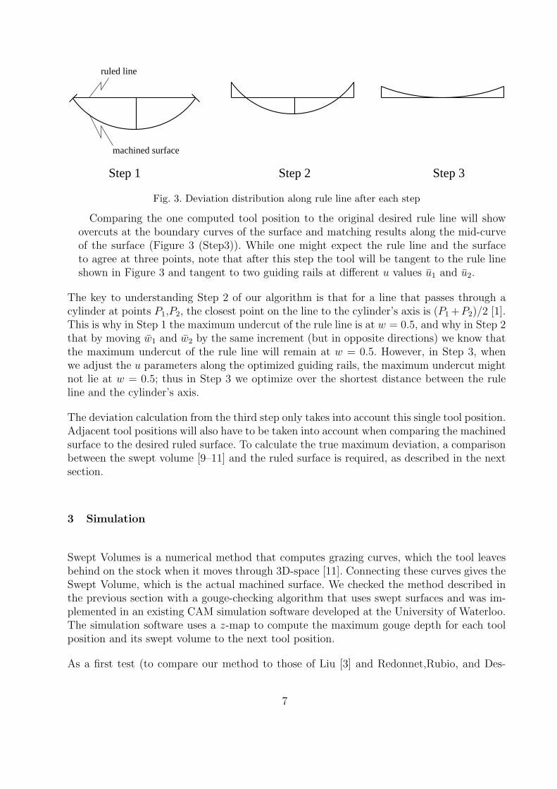
Step 1 Step 2 Step 3

ruled line

machined surface

Fig. 3. Deviation distribution along rule line after each step

Comparing the one computed tool position to the original desired rule line will showovercuts at the boundary curves of the surface and matching results along the mid-curveof the surface (Figure 3 (Step3)). While one might expect the rule line and the surfaceto agree at three points, note that after this step the tool will be tangent to the rule lineshown in Figure 3 and tangent to two guiding rails at different u values u1 and u2.

The key to understanding Step 2 of our algorithm is that for a line that passes through acylinder at points P1,P2, the closest point on the line to the cylinder’s axis is (P1 +P2)/2 [1].This is why in Step 1 the maximum undercut of the rule line is at w = 0.5, and why in Step 2that by moving w1 and w2 by the same increment (but in opposite directions) we know thatthe maximum undercut of the rule line will remain at w = 0.5. However, in Step 3, whenwe adjust the u parameters along the optimized guiding rails, the maximum undercut mightnot lie at w = 0.5; thus in Step 3 we optimize over the shortest distance between the ruleline and the cylinder’s axis.

The deviation calculation from the third step only takes into account this single tool position.Adjacent tool positions will also have to be taken into account when comparing the machinedsurface to the desired ruled surface. To calculate the true maximum deviation, a comparisonbetween the swept volume [9–11] and the ruled surface is required, as described in the nextsection.

3 Simulation

Swept Volumes is a numerical method that computes grazing curves, which the tool leavesbehind on the stock when it moves through 3D-space [11]. Connecting these curves gives theSwept Volume, which is the actual machined surface. We checked the method described inthe previous section with a gouge-checking algorithm that uses swept surfaces and was im-plemented in an existing CAM simulation software developed at the University of Waterloo.The simulation software uses a z-map to compute the maximum gouge depth for each toolposition and its swept volume to the next tool position.

As a first test (to compare our method to those of Liu [3] and Redonnet,Rubio, and Des-

7

Table 1Control points for Liu surface [mm]

T0 = (0; 0; 33.995) T1 = (11.507; 0; 33.995) T2 = (23.014; 20.2324; 33.995)

B0 = (0; 20.429; 0) B1 = (11.507; 20.429; 0) B2 = (23.014; 20.429; 0)

sein [4]) we use the surface given in Liu’s paper as the two rails

T (u) =

u

20.429

0

B(u) =

u

0.0382u2

33.995

with 0 ≤ u ≤ 23.014 and 0 ≤ v ≤ 1. The quadratic Bezier control points for these curvesappear in Table 1. In the examples, the surface is machined with a cylindrical tool withradius of 10mm.

In Table 2 we give the maximum undercut and overcut of four methods on Liu’s surface.The values for Liu’s and Redonnet-Rubio-Dessein’s methods are taken from their papers.This makes a direct comparison a bit more difficult because of the different methods used tocompute the errors. In particular, the values for Liu’s method was computed by comparing arule line to the corresponding tool position, while the values we give for Bedi-Mann-Menzel’smethod and for the method described in this paper were computed as the maximum distancebetween the rule lines and the swept surface. Redonnet-Rubio-Dessein computed the errorby looking at two successive positions rather than the entire swept surface.

For the Bedi-Mann-Menzel method and for the method described in this paper, we used atoolpath comprised of 100 tool positions. In the table, we give the maximum error after eachof the three steps of our method. The error appearing in the first column (Step 1) is alsothe error of the earlier Bedi-Mann-Menzel method. The error of the complete method is thatappearing under the Step 3 column. Roughly speaking, our new method has error comparableto Redonnet-Rubio-Dessein’s method, which is to be expected since both methods place thetool tangent to the rule line and to two other curves on the ruled surface.

For the method described in this paper, in addition to the maximum error, we also give themaximum angle change between adjacent tool positions (such values were not available forthe other two methods).

The test surface in Liu’s paper is fairly simple: one rail is a straight line, while the other is aquadratic curve. As a second test, we designed three ruled surfaces to compare the deviationsbetween Bedi et al.’s strategy to the deviations achieved with the optimized method discussedin this paper. One surface has two concave-up curves, the second has one concave-up and oneconcave-down curve, and the third surface has two concave-down curves. Each ruled surfaceis comprised of two quadratic Bezier curves; a top curve T (u) and a bottom curve B(u).The control points for the quadratic guiding rails are given in Table 3 and the ruled surfaces

8

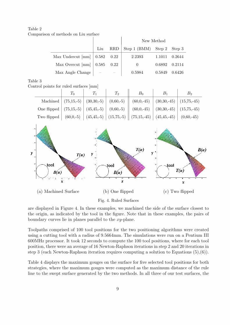
Table 2Comparison of methods on Liu surface

New Method

Liu RRD Step 1 (BMM) Step 2 Step 3

Max Undercut [mm] 0.582 0.22 2.2393 1.1011 0.2644

Max Overcut [mm] 0.585 0.22 0 0.6892 0.2114

Max Angle Change – – 0.5984 0.5849 0.6426

Table 3Control points for ruled surfaces [mm]

T0 T1 T2 B0 B1 B2

Machined (75,15,-5) (30,30,-5) (0,60,-5) (60,0,-45) (30,30,-45) (15,75,-45)

One flipped (75,15,-5) (45,45,-5) (0,60,-5) (60,0,-45) (30,30,-45) (15,75,-45)

Two flipped (60,0,-5) (45,45,-5) (15,75,-5) (75,15,-45) (45,45,-45) (0,60,-45)

(a) Machined Surface (b) One flipped (c) Two flipped

Fig. 4. Ruled Surfaces

are displayed in Figure 4. In these examples, we machined the side of the surface closest tothe origin, as indicated by the tool in the figure. Note that in these examples, the pairs ofboundary curves lie in planes parallel to the xy-plane.

Toolpaths comprised of 100 tool positions for the two positioning algorithms were createdusing a cutting tool with a radius of 9.5664mm. The simulations were run on a Pentium III600MHz processor. It took 12 seconds to compute the 100 tool positions, where for each toolposition, there were an average of 16 Newton-Raphson iterations in step 2 and 20 iterations instep 3 (each Newton-Raphson iteration requires computing a solution to Equations (5),(6)).

Table 4 displays the maximum gouges on the surface for five selected tool positions for bothstrategies, where the maximum gouges were computed as the maximum distance of the ruleline to the swept surface generated by the two methods. In all three of our test surfaces, the

9

Table 4Comparison of methods

Maximum deviation (mm)

Machined example One curve flipped Both curves flipped

Position Bedi Optimized Bedi Optimized Bedi Optimized

undercut 0.2899 0.0061 0.8339 0.0099 0.2876 0.0061

overcut 0 0.0063 0 0.0169 0 0.0091

Maximum angle change between adjacent positions (degrees)

0.6353 0.6225 0.9772 0.9846 0.5727 0.5906

maximum gouging was reduced by more than 97%. We also computed the overcut of the twomethods. Bedi et al.’s method will have 0 overcut, since the segment of interest of the ruleline lies entirely inside the tool. The optimization method described in this paper has a non-zero overcut; however, as seen in Table 4, for our examples this overcut is nearly two ordersof magnitude smaller than the undercut of the Bedi et al. method. We also machined thesurface appearing in Figure 4(a) using both Bedi et al.’s method and the method describedin this paper; details on the machining appear in the next section.

This comparison shows that gouges were significantly reduced on the whole surface with theoptimized method. The gouging regions produced by both methods were computed with thesimulation software and are displayed qualitatively in Figure 5. Note that Figure 3, Step 3might suggest that there should be no undercut. However, this figure compares the tool toa particular rule line, while the tool is actually tangent to two other curves at different uvalues. Thus, as indicated in Table 4, there will be some undercutting.

A few notes on our method as revealed by the simulations are in order. First, note thew parameters w1 and w2 give the two isoparametric curves to which the tool is tangent.Initially, w1 = 0 and w2 = 1, which we adjust in step 2 of our algorithm to equalize theovercut and undercut. The only restrictions we place on these two values is w1 ∈ [0, 0.5] andw2 ∈ [0.5, 1]. However, in our simulations, the optimization settled on values near 0.14 and0.86 respectively, and never approached the ends of these intervals.

A second note regards the optimized u parameters and the angle of the tool axis. In step 1of our algorithm, we use the same u value for both points of tangency. In step 3 of ouralgorithm, we adjust the two u values in opposite directions to make the tool tangent to twoisoparametric lines and tangent to the rule line. A comparison of the tool axis given in thefirst step (i.e., by Bedi et al.’s method) to our method showed in our examples a change inangle by as much as 5 degrees. However, as shown in the last line of Table 4, the maximumchange in the tool axis angle between adjacent tool positions within one method was lessthan 1 degree.

Finally, note that the optimization method reduces the error between a single tool positionand a single rule line at parameter value u. Potentially, the tool at one position u might

10

(a) Bedi et al.’s method (b) Optimized method

Fig. 5. Graphical simulation of the two positioning strategies

Fig. 6. Comparison of measured data with designed ruled surface (w = 0.5)

significantly cut another, nearby rule line at parameter value u′ = u + ε. We did not see thisproblem in the swept volume analysis of our examples.

4 Machining Test

A machining test was conducted to confirm the simulation results. Two parts were flankmilled with a flat end cutter on a Deckel Maho 80Pi Hi-Dyn five-axis machine using the twotoolpaths described in the simulation section (i.e., one was machined with Bedi et al. method,while the other was machined with the new method described in this paper). Measurementsalong the mid-curve of the machined surfaces were taken and compared to each other. Thedeviation of the machined mid-curves from the designed ruled surface is displayed in Figure 6.In this figure, we have graphed a portion of the w = 0.5 curves; only the x,y values of thecurves are shown since all the curves have the same z-values because the boundary curveslie in planes parallel to the xy-plane. The depicted sections of the mid-curve show that themachining results match closely to the expected simulation results at tool position number50 (see Table 4).

11

Fig. 7. Machined Part, where T is the top curve and B is the bottom curve.

5 Conclusions

In flank milling most research work focuses on machining ruled surfaces. Several positioningstrategies have been developed to minimize the deviations between the design surface andthe actual machined surface. The main goal of this study was to develop and implement anoptimized method for flank milling ruled surfaces. Our method was based on the earlier workof Bedi et al. [1], which gave a method for placing a cylindrical tool tangent to two, fixedguiding rails.

For the optimized method, the guiding rails at which the cutting tool and ruled surface arepositioned tangential to each other are no longer restricted to the two boundary curves, butcan be located anywhere on the ruled surface. The new algorithm will find the optimumguiding rails for which the deviation is minimized. Placing the tool tangential to these opti-mum guiding rails leads to three tangency points for each tool position: one point on eachoptimized guiding rail and the third point on the rule line.

The optimized method reduces the deviation by more than 88% compared to the strategyproposed by Bedi et al. Furthermore, only two equations need to be solved for numerically,which makes the algorithm computationally inexpensive and robust.

6 Acknowledgements

This work was funded in part by NSERC, CFI, and OIT.

12

References

[1] S. Bedi, S. Mann, and C. Menzel. Flank milling with flat end cutters. Computer Aided Design,35:293–300, 2003.

[2] E. L. J. Bohez, S. D. R. Senadhera, K. Pole, J. R. Duflou, and T. Tar. A geometric modelingand five-axis machining algorithm for centrifugal impellers. Journal of Manufacturing Systems,16(6):422–463, 1997.

[3] X. W. Liu. Five-axis NC cylindrical milling of sculptured surfaces. Computer-Aided Design,27(12):887–894, 1995.

[4] J.-M. Redonnet, W. Rubio, and G. Dessein. Side milling of ruled surfaces: Optimum positioningof the milling cutter and calculation of interference. International Journal for AdvancedManufacturing Technology, 14:459–465, 1998.

[5] F. Rehsteiner and H. J. Renker. Collision free five axis milling of twisted ruled surfaces. Annalsof CIRP, 42(1):267–271, 1993.

[6] H. K. Tonshoff and N. Rackow. A CAM software prototype for five axis flank milling free-formsurfaces. In Proceedings of the Third International Conference on Metal Cutting and High SpeedMachining, pages 139–147, June 2001.

[7] C. W. Wu. Arbitrary surface flank milling of fan, compressor, and impeller blades. Journal ofEngineering for Gas Turbines and Power, 117:534–539, July 1995.

[8] D. M. Tsay and M. J. Her. Accurate 5-axis machining of twisted ruled surfaces. Journal ofManufacturing Science and Engineering, 123:731–738, 2001.

[9] K. Sheltami, S. Bedi, and F. Ismail. Swept volumes of toroidal cutters using generating curves.International Journal of Machine Tools and Manufacture, 38:855–870, 1998.

[10] D. Roth, S. Bedi, F. Ismail, and S. Mann. Surface swept by a toroidal cutter during 5-axismachining. Computer Aided Design, 33(1):57–63, 2001.

[11] D. J. Roth. Surface swept by a toroidal cutter during 5-axis machining of curved surfacesand its application to gouge checking. Master’s thesis, Mechanical Engineering, University ofWaterloo, 1999.

13