Transformation invariance in pattern recognition -

tangent distance and tangent propagation

Patrice Simard, Yann Le Cun, John Denker, Bernard Victorri

To cite this version:

Patrice Simard, Yann Le Cun, John Denker, Bernard Victorri. Transformation invariancein pattern recognition - tangent distance and tangent propagation. Neural Networks: Trickson the Trade, 1524, Springer-Verlag, pp.239-274, 1998, Lectures Notes in Computer Science.<halshs-00009505>

HAL Id: halshs-00009505

https://halshs.archives-ouvertes.fr/halshs-00009505

Submitted on 8 Mar 2006

HAL is a multi-disciplinary open accessarchive for the deposit and dissemination of sci-entific research documents, whether they are pub-lished or not. The documents may come fromteaching and research institutions in France orabroad, or from public or private research centers.

L’archive ouverte pluridisciplinaire HAL, estdestinee au depot et a la diffusion de documentsscientifiques de niveau recherche, publies ou non,emanant des etablissements d’enseignement et derecherche francais ou etrangers, des laboratoirespublics ou prives.

Transformation Invariance in Pattern

Recognition { Tangent Distance and Tangent

Propagation

Patrice Y. Simard1, Yann A. Le Cun1, John S. Denker1, Bernard Victorri2

1 Image Processing Services Research Lab, AT& T Labs - Research, 100 SchulzDrive, Red Bank, NJ 07701-7033, USA

2 Universite de Caen, Esplanade de la Paix - 14032 Caen Cedex - France

Abstract. In pattern recognition, statistical modeling, or regression,the amount of data is the most critical factor a�ecting the performance.If the amount of data and computational resources are near in�nite,many algorithms will provably converge to the optimal solution. Whenthis is not the case, one has to introduce regularizers and a-priori knowl-edge to supplement the available data in order to boost the performance.Invariance (or known dependence) with respect to transformation of theinput is a frequent occurrence of such a-priori knowledge. In this chapter,we introduce the concept of tangent vectors, which compactly representthe essence of these transformation invariances, and two classes of algo-rithms, \Tangent distance" and \Tangent propagation", which make useof these invariances to improve performance.

1 Introduction

Pattern Recognition is one of the main tasks of biological information process-ing systems, and a major challenge of computer science. The problem of patternrecognition is to classify objects into categories, given that objects in a particu-lar category may vary widely, while objects in di�erent categories may be verysimilar. A typical example is handwritten digit recognition. Characters, typicallyrepresented as �xed-size images (say 16 by 16 pixels), must be classi�ed into oneof 10 categories using a classi�cation function. Building such a classi�cation func-tion is a major technological challenge, as variabilities among objects of the sameclass must be eliminated, while di�erences between objects of di�erent classesmust be identi�ed. Since classi�cation functions for most real pattern recognitiontasks are too complicated to be synthesized \by hand", automatic techniquesmust be devised to construct the classi�cation function from a set of labeledexamples (the training set). These techniques can be divided into two camps,according to the number of parameters they are requiring: the \memory based"algorithms, which use a (compact) representation of the training set, and the\learning" techniques, which require adjustments of a comparatively small num-ber of parameters (during training) to compute the classi�cation function. Thisdistinction can be somewhat arbitrary because some classi�cation algorithms,

for instance Learning vector quantization or LVQ, are hybrids. The distinctionserves our purpose, nonetheless, because memory based algorithms often relyon a metric which can be modi�ed to incorporate transformation invariances,while learning based algorithms consist of selecting a classi�cation function, thederivatives of which can be constrained to re ect the same transformation in-variances. The two methods for incorporating invariances are di�erent enoughto justify two independent sections.

1.1 Memory based algorithms

To compute the classi�cation function, many practical pattern recognition sys-tems, and several biological models, simply store all the examples, together withtheir labels, in a memory. Each incoming pattern can then be compared to allthe stored prototypes, and the label associated with the prototype that bestmatches the input can be output-ed. The above method is the simplest exampleof the memory-based models. Memory-based models require three things: a dis-

tance measure to compare inputs to prototypes, an output function to producean output by combining the labels of the prototypes, and a storage scheme tobuild the set of prototypes.

All three aspects have been abundantly treated in the literature. Outputfunctions range from simply voting the labels associated with the k closest pro-totypes (K-Nearest Neighbors), to computing a score for each class as a linearcombination of the distances to all the prototypes, using �xed [21] or learned [5]coe�cients. Storage schemes vary from storing the entire training set, to pickingappropriate subsets of it (see [8], chapter 6, for a survey) to learning algorithmssuch as Learning Vector Quantization (LVQ) [17] and gradient descent. Distancemeasures can be as simple as the Euclidean distance, assuming the patterns andprototypes are represented as vectors, or more complex as in the generalizedquadratic metric [10] or in elastic matching methods [15].

Pattern tobe classified Prototype A Prototype B

Fig. 1. According to the Euclidean distance the pattern to be classi�ed is more similarto prototype B. A better distance measure would �nd that prototype A is closer becauseit di�ers mainly by a rotation and a thickness transformation, two transformationswhich should leave the classi�cation invariant.

A simple but ine�cient pattern recognition method is to combine a simpledistance measure, such as Euclidean distance between vectors, with a very large

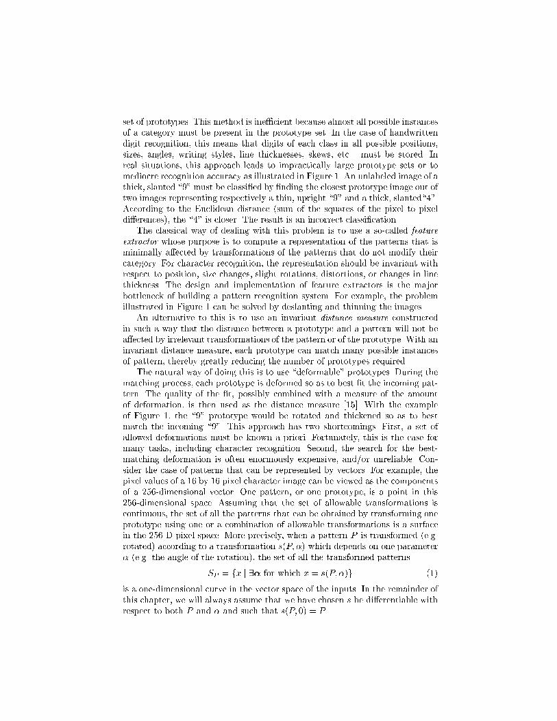
set of prototypes. This method is ine�cient because almost all possible instancesof a category must be present in the prototype set. In the case of handwrittendigit recognition, this means that digits of each class in all possible positions,sizes, angles, writing styles, line thicknesses, skews, etc... must be stored. Inreal situations, this approach leads to impractically large prototype sets or tomediocre recognition accuracy as illustrated in Figure 1. An unlabeled image of athick, slanted \9" must be classi�ed by �nding the closest prototype image out oftwo images representing respectively a thin, upright \9" and a thick, slanted\4".According to the Euclidean distance (sum of the squares of the pixel to pixeldi�erences), the \4" is closer. The result is an incorrect classi�cation.

The classical way of dealing with this problem is to use a so-called feature

extractor whose purpose is to compute a representation of the patterns that isminimally a�ected by transformations of the patterns that do not modify theircategory. For character recognition, the representation should be invariant withrespect to position, size changes, slight rotations, distortions, or changes in linethickness. The design and implementation of feature extractors is the majorbottleneck of building a pattern recognition system. For example, the problemillustrated in Figure 1 can be solved by deslanting and thinning the images.

An alternative to this is to use an invariant distance measure constructedin such a way that the distance between a prototype and a pattern will not bea�ected by irrelevant transformations of the pattern or of the prototype. With aninvariant distance measure, each prototype can match many possible instancesof pattern, thereby greatly reducing the number of prototypes required.

The natural way of doing this is to use \deformable" prototypes. During thematching process, each prototype is deformed so as to best �t the incoming pat-tern. The quality of the �t, possibly combined with a measure of the amountof deformation, is then used as the distance measure [15]. With the exampleof Figure 1, the \9" prototype would be rotated and thickened so as to bestmatch the incoming \9". This approach has two shortcomings. First, a set ofallowed deformations must be known a priori. Fortunately, this is the case formany tasks, including character recognition. Second, the search for the best-matching deformation is often enormously expensive, and/or unreliable. Con-sider the case of patterns that can be represented by vectors. For example, thepixel values of a 16 by 16 pixel character image can be viewed as the componentsof a 256-dimensional vector. One pattern, or one prototype, is a point in this256-dimensional space. Assuming that the set of allowable transformations iscontinuous, the set of all the patterns that can be obtained by transforming oneprototype using one or a combination of allowable transformations is a surfacein the 256-D pixel space. More precisely, when a pattern P is transformed (e.g.rotated) according to a transformation s(P; �) which depends on one parameter� (e.g. the angle of the rotation), the set of all the transformed patterns

SP = fx j 9� for which x = s(P; �)g (1)

is a one-dimensional curve in the vector space of the inputs. In the remainder ofthis chapter, we will always assume that we have chosen s be di�erentiable withrespect to both P and � and such that s(P; 0) = P .

When the set of transformations is parameterized by n parameters �i (ro-tation, translation, scaling, etc.), the intrinsic dimension of the manifold SP isat most n. For example, if the allowable transformations of character imagesare horizontal and vertical shifts, rotations, and scaling, the surface will be a4-dimensional manifold.

In general, the manifold will not be linear. Even a simple image translationcorresponds to a highly non-linear transformation in the high-dimensional pixelspace. For example, if the image of a \8" is translated upward, some pixelsoscillate from white to black and back several times. Matching a deformableprototype to an incoming pattern now amounts to �nding the point on the sur-face that is at a minimum distance from the point representing the incomingpattern. Because the manifold is non-linear, the matching can be very expen-sive and unreliable. Simple minimization methods such as gradient descent (orconjugate gradient) can be used to �nd the minimum-distance point, however,these methods only converge to a local minimum. In addition, running such aniterative procedure for each prototype is prohibitively expensive.

If the set of transformations happens to be linear in pixel space, then themanifold is a linear subspace (a plane). The matching procedure is then reducedto �nding the shortest distance between a point (vector) and a plane: an easy-to-solve quadratic minimization problem. This special case has been studied in thestatistical literature and is sometimes referred to as Procrustes analysis [24]. Ithas been applied to signature veri�cation [12] and on-line character recognition[26].

This chapter considers the more general case of non-linear transformationssuch as geometric transformations of gray-level images. Remember that even asimple image translation corresponds to a highly non-linear transformation inthe high-dimensional pixel space. The main idea of the chapter is to approx-imate the surface of possible transforms of a pattern by its tangent plane atthe pattern, thereby reducing the matching to �nding the shortest distance be-tween two planes. This distance is called the Tangent Distance. The result ofthe approximation is shown in Figure 2, in the case of rotation for handwrittendigits. At the top of the �gure, is the theoretical curve in pixel space whichrepresents equation (1), together with its linear approximation. Points of thetransformation curve are depicted below for various amounts of rotation (eachangle corresponds to a value of �). The bottom of Figure 2 depicts the linearapproximation of the curve s(P; �) given by the Taylor expansion of s around� = 0:

s(P; �) = s(P; 0) + �@s(P; �)

@�+O(�2) � P + �T (2)

This linear approximation is completely characterized by the point P and the

tangent vector T = @s(P;�)@�

. Tangent vectors, also called the Lie derivatives of thetransformation s, will be the subject of section 4. As can be seen from Figure 2,for small angles (k�k < 1), the approximation is very good.

Figure 3 illustrates the di�erence between the Euclidean distance, the fullinvariant distance (minimum distance between manifolds) and the tangent dis-tance. In the �gure, both the prototype and the pattern are deformable (two-

),

+ .

=α

=α

α=1α=−2 α=−1 α=0 α=2

P

α α=0

α=1

α=−2α=−1

α=2

T

P+ .Tα

Pixel space

TP

∂∂ α=T

s(P, )

s(

s

Fig. 2. Top: Representation of the e�ect of the rotation in pixel space. Middle: Smallrotations of an original digitized image of the digit \2", for di�erent angle values of�. Bottom: Images obtained by moving along the tangent to the transformation curvefor the same original digitized image P by adding various amounts (�) of the tangentvector T .

sided distance), but for simplicity or e�ciency reasons, it is also possible todeform only the prototype or only the unknown pattern (one-sided distance).

Although in the following we will concentrate on using tangent distance torecognize images, the method can be applied to many di�erent types of signals:temporal signals, speech, sensor data...

1.2 Learning based algorithms

Rather than trying to keep a representation of the training set, it is also possibleto compute the classi�cation function by learning a set of parameters from the�nite training set. This is the approach taken in neural networks. Let F (x) bethe (unknown) function to be learned, B = f(x1; F (x1)); : : : ; (xp; F (xp))g be a�nite set of training data taken from a constant statistical distribution P , andlet Gw(x) be a set of functions, indexed by the vector of parameters w. The task

E

Euclidean distancebetween P and E

PTangent Distance

Distance betweenS and S

S

SP E

P

E

Fig. 3. Illustration of the Euclidean distance and the tangent distance between P andE. The curves Sp and Se represent the sets of points obtained by applying the chosentransformations (for example translations and rotations) to P and E. The lines goingthrough P and E represent the tangent to these curves. Assuming that working spacehas more dimensions than the number of chosen transformations (on the diagram,assume 3D) the tangent spaces do not intersect and the tangent distance is uniquelyde�ned.

is to �nd a value for w from the �nite training data set B such that Gw bestapproximates F on its input x. For example, Gw may be the function computedby a neural net and the vector w may be the neural net's weights, or Gw maybe a polynomial and w its coe�cients. Without additional information, �ndinga value for w is an ill-posed problem because the training set does not provideenough information to distinguish the best solution among all the candidatesws. This problem is illustrated in Figure 4 (left). The desired function F (solidline) is to be approximated by a functions Gw (dotted line) from four examplesf(xi; F (xi))gi=1;2;3;4. As exempli�ed in the picture, the �tted functionGw largelydisagrees with the desired function F between the examples, but it is not possibleto infer this from the training set alone. Many values of w can generate manydi�erent function Gw, some of which may be terrible approximations of F , eventhough they are in complete agreement with the training set. Because of this,it is customary to add \regularizers", or additional constraints, to restrict thesearch of an acceptable w. For example, we may require the function Gw tobe \smooth", by adding the constraint that kwk2 should be minimized. It isimportant that the regularizer re ects a property of F , hence regularizers requireadditional a-priori knowledge about the function to be modeled.

x2x1 x3 x4

F(x)

x x2x1 x3 x4

F(x)

x

wG (x)

wG (x)

Fig. 4. Learning a given function (solid line) from a limited set of examples (x1 to x4).The �tted curves are shown by dotted line. Left: The only constraint is that the �ttedcurve goes through the examples. Right: The �tted curves not only go through eachexample but also its derivatives evaluated at the examples agree with the derivativesof the given function.

Selecting a good family G = fGw; w 2 <qg of functions is a di�cult task,sometimes known as \model selection" [16, 14]. If G contains a large family offunctions, it is more likely that it will contain a good approximation of F (thefunction we are trying to approximate), but it is also more likely that the selectedcandidate (using the training set) will generalize poorly because many functionsin G will agree with the training data and take outrageous values between thetraining samples. If, on the other hand, G contains a small family of functions, itis more likely that a functionGw which �ts the data will be a good approximationof F . The capacity of the family of functions G is often referred to as the VCdimension [28, 27]. If a large amount of data is available, G should contain alarge family of functions (high VC dimension), so that more functions can beapproximated, and in particular, F . If, on the other hand, the data is scarce, Gshould be restricted to a small family of functions (low VC dimension), to controlthe values between the (more distant) samples1. The VC dimension can also becontrolled by putting a knob on how much e�ect is given to some regularizers.For instance it is possible to control the capacity of a neural network by adding\weight decay" as a regularizer. Weight decay is a loose smoothness constrainton the classi�cation function which works by decreasing kwk2 as well as the erroron the training set. Since the classi�cation function is not necessarily smooth, forinstance at a decision boundary, the weight decay regularizer can have adversee�ects.

As mentioned earlier, the regularizer should re ect interesting properties (apriori knowledge) of the function to be learned. If the functions F and Gw areassumed to be di�erentiable, which is generally the case, the search forGw can be

1 Note that this formalism could also be used for memory based system. In the casewhere all the training data can be kept in memory, however, the VC dimension isin�nite, and the formalism is meaningless. The VC dimension is a learning paradigmand is not useful unless learning is involved.

greatly improved by requiring that Gw 's derivatives evaluated at the points fxigare more or less equal (this is the regularizer knob) to the derivatives of F at thesame points (Figure 4 right). This result can be extended to multidimensionalinputs. In this case, we can impose the equality of the derivatives of F and Gw

in certain directions, not necessarily in all directions of the input space.

Such constraints �nd immediate use in traditional learning pattern recogni-tion problems. It is often the case that a priori knowledge is available on how thedesired function varies with respect to some transformations of the input. It isstraightforward to derive the corresponding constraint on the directional deriva-tives of the �tted function Gw in the directions of the transformations (previouslynamed tangent vectors). Typical examples can be found in pattern recognitionwhere the desired classi�cation function is known to be invariant with respectto some transformation of the input such as translation, rotation, scaling, etc.,in other words, the directional derivatives of the classi�cation function in thedirections of these transformations is zero.

This is illustrated in Figure 4. The right part of the �gure shows how theadditional constraints onGw help generalization by constraining the values ofGw

outside the training set. For every transformation which has a known e�ect onthe classi�cation function, a regularizer can be added in the form of a constrainton the directional derivative of Gw in the direction of the tangent vector (suchas the one depicted in Figure 2), computed from the curve of transformation.

The next section will analyze in detail how to use a distance based on tangentvector in memory based algorithms. The subsequent section will discuss the useof tangent vectors in neural network, with the tangent propagation algorithm.The last section will compare di�erent algorithms to compute tangent vectors.

2 Tangent Distance

The Euclidean distance between two patterns P and E is in general not ap-propriate because it is sensitive to irrelevant transformations of P and of E. Incontrast, the distance D(E;P ) de�ned to be the minimal distance between thetwo manifolds SP and SE is truly invariant with respect to the transformationused to generate SP and SE (see Figure 3). Unfortunately, these manifolds haveno analytic expression in general, and �nding the distance between them is adi�cult optimization problem with multiple local minima. Besides, true invari-ance is not necessarily desirable since a rotation of a \6" into a \9" does notpreserve the correct classi�cation.

Our approach consists of computing the minimum distance between the linearsurfaces that best approximate the non-linear manifolds SP and SE . This solvesthree problems at once: 1) linear manifolds have simple analytical expressionswhich can be easily computed and stored, 2) �nding the minimum distancebetween linear manifolds is a simple least squares problem which can be solvede�ciently and, 3) this distance is locally invariant but not globally invariant.Thus the distance between a \6" and a slightly rotated \6" is small but the

distance between a \6" and a \9" is large. The di�erent distances between Pand E are represented schematically in Figure 3.

The �gure represents two patterns P and E in 3-dimensional space. The man-ifolds generated by s are represented by one-dimensional curves going through Eand P respectively. The linear approximations to the manifolds are representedby lines tangent to the curves at E and P . These lines do not intersect in 3 di-mensions and the shortest distance between them (uniquely de�ned) is D(E;P ).The distance between the two non-linear transformation curves D(E;P ) is alsoshown on the �gure.

An e�cient implementation of the tangent distance D(E;P ) will be givenin the next section. Although the tangent distance can be applied to any kindof patterns represented as vectors, we have concentrated our e�orts on applica-tions to image recognition. Comparison of tangent distance with the best knowncompeting method will be described. Finally we will discuss possible variationson the tangent distance and how it can be generalized to problems other thanpattern recognition.

2.1 Implementation

In this section we describe formally the computation of the tangent distance. Letthe function s transform an image P to s(P; �) according to the parameter �. Werequire s to be di�erentiable with respect to � and P , and require s(P; 0) = P .If P is a 2 dimensional image for instance, s(P; �) could be a rotation of P bythe angle �. If we are interested in all transformations of images which conservedistances (isometry), s(P; �) would be a rotation by �� followed by a translationby �x; �y of the image P . In this case � = (��; �x; �y) is a vector of parametersof dimension 3. In general, � = (�1; : : : ; �m) is of dimension m.

Since s is di�erentiable, the set SP = fx j 9� for which x = s(P; �)g isa di�erentiable manifold which can be approximated to the �rst order by ahyperplane TP . This hyperplane is tangent to SP at P and is generated by thecolumns of matrix

LP =@s(P; �)

@�

�����=0

=

�@s(P; �)

@�1; : : : ;

@s(P; �)

@�m

��=0

(3)

which are vectors tangent to the manifold. If E and P are two patterns to becompared, the respective tangent planes TE and TP can be used to de�ne a newdistance D between these two patterns. The tangent distance D(E;P ) betweenE and P is de�ned by

D(E;P ) = minx2TE;y2TP

kx� yk2 (4)

The equation of the tangent planes TE and TP is given by:

E0(�E) = E + LE�E (5)

P 0(�P ) = P + LP�P (6)

where LE and LP are the matrices containing the tangent vectors (see equa-tion (3)) and the vectors �E and �P are the coordinates of E0 and P 0 (usingbases LE and LP ) in the corresponding tangent planes. Note that E0, E, LEand �E denote vectors and matrices in linear equations (5). For example, if thepixel space was of dimension 5, and there were two tangent vectors, we couldrewrite equation (5) as2

66664

E01E02E03E04E05

377775 =

266664

E1

E2

E3

E4

E5

377775 +

266664

L11 L12L21 L22L31 L32L41 L42L51 L52

377775��1�2

�(7)

The quantities LE and LP are attributes of the patterns so in many cases theycan be precomputed and stored.

Computing the tangent distance

D(E;P ) = min�E;�P

kE0(�E)� P 0(�P )k2 (8)

amounts to solving a linear least squares problem. The optimality condition isthat the partial derivatives of D(E;P ) with respect to �P and �E should bezero:

@D(E;P )

@�E= 2(E0(�E)� P 0(�P ))

>LE = 0 (9)

@D(E;P )

@�P= 2(P 0(�P )�E0(�E))

>LP = 0 (10)

Substituting E0 and P 0 by their expressions yields to the following linear systemof equations, which we must solve for �P and �E :

L>P (E � P � LP�P + LE�E) = 0 (11)

L>E(E � P � LP�P + LE�E) = 0 (12)

The solution of this system is

(LPEL�1EEL

>E � L>P )(E � P ) = (LPEL

�1EELEP � LPP )�P (13)

(LEPL�1PPL

>P � L>E)(E � P ) = (LEE � LEPL

�1PPLPE)�E (14)

where LEE = L>ELE , LPE = L>PLE , LEP = L>ELP and LPP = L>PLP . LUdecompositions of LEE and LPP can be precomputed. The most expensive partin solving this system is evaluating LEP (LPE can be obtained by transposingLEP ). It requires mE �mP dot products, where mE is the number of tangentvectors for E and mP is the number of tangent vectors for P . Once LEP hasbeen computed, �P and �E can be computed by solving two (small) linearsystems of respectively mE and mP equations. The tangent distance is obtainedby computing kE0(�E)�P

0(�P )k using the value of �P and �E in equations (5)and (6). If n is the dimension of the input space (i.e. the length of vector Eand P ), the algorithm described above requires roughly n(mE + 1)(mP + 1) +3(m3

E+m3P ) multiply-adds. Approximations to the tangent distance can however

be computed more e�ciently.

2.2 Some illustrative results

Local Invariance: The \local invariance2" of tangent distance can be illus-trated by transforming a reference image by various amounts and measuring itsdistance to a set of prototypes.

−6 −5 −4 −3 −2 −1 0 1 2 3 4 5 6−6 −5 −4 −3 −2 −1 0 1 2 3 4 5 60

2

4

6

8

10

12

0

2

4

6

8

10

12

0 1

2

3

4

5

6

7

89

0

1

2

3

4

5

6

7

89

Euclidean Distance Tangent Distance

Fig. 5. Euclidean and tangent distances between 10 typical handwritten images of the10 digits (10 curves) and a digit image translated horizontally by various amounts(indicated in absyssa, in pixel). On the �gure the translated image is the digit \3"from the 10 digits above.

On Figure 5, 10 typical handwritten digit images are selected (bottom), andone of them { the digit \3" { is chosen to be the reference. The reference istranslated from 6 pixels to the left, to 6 pixels to the right, and the translationamount is indicated in absyssa. Each curve represents the Euclidean Distance(or the Tangent Distance) between the (translated) reference and one of the 10digits.

Since the reference was chosen from the 10 digits, it is not surprising thatthe curve corresponding to the digit \3" goes to 0 when the reference is nottranslated (0 pixel translation). It is clear from the �gure that if the reference

2 Local invariance refers to invariance with respect to small transformations (i.e. arotation of a very small angle). In contrast, global invariance refers to invariancewith respect to arbitrarily large transformations (i.e. a rotation of 180 degrees).Global invariance is not desirable in digit recognition, since we need to distinguish\6"s and \9"s.

(the image \3") is translated by more than 2 pixels, the Euclidean Distance willconfuse it with other digits, namely \8" or \5". In contrast, there is no possibleconfusion when Tangent Distance is used. As a matter of fact, in this example,the Tangent Distance correctly identi�es the reference up to a translation of 5pixels! Similar curves were obtained with all the other transformations (rotation,scaling, etc...).

The \local" invariance of Tangent distance with respect to small transforma-tions generally implies more accurate classi�cation for much larger transforma-tions. This is the single most important feature of Tangent Distance.

Original

Tangent vectors Points in the tangent plane

Fig. 6. Left: Original image. Middle: 5 tangent vectors corresponding respectively tothe 5 transformations: scaling, rotation, expansion of the X axis while compressingthe Y axis, expansion of the �rst diagonal while compressing the second diagonal andthickening. Right: 32 points in the tangent space generated by adding or subtractingeach of the 5 tangent vectors.

The locality of the invariance has another important bene�t: Local invariancecan be enforced with very few tangent vectors. The reason is that for in�nitesimal(local) transformations, there is a direct correspondence3 between the tangentvectors of the tangent plane and the various compositions of transformations. Forexample, the three tangent vectors for X-translation, Y-translation and rotationsof center O, generate a tangent plane corresponding to all the possible composi-tions of horizontal translations, vertical translations and rotations of center O.The resulting tangent distance is then locally invariant to all the translations andall the rotations (of any center). Figure 6 further illustrates this phenomenon bydisplaying points in the tangent plane generated from only 5 tangent vectors.

3 an isomorphism actually, see \Lie algebra" in [6]

Each of these images looks like it has been obtained by applying various com-binations of scaling, rotation, horizontal and vertical skewing, and thickening.Yet, the tangent distance between any of these points and the original image is0.

Handwritten Digit Recognition: Experiments were conducted to evaluatethe performance of tangent distance for handwritten digit recognition. An inter-esting characteristic of digit images is that we can readily identify a set of localtransformations which do not a�ect the identity of the character, while coveringa large portion of the set of possible instances of the character. Seven such im-age transformations were identi�ed: X and Y translations, rotation, scaling, twohyperbolic transformations (which can generate shearing and squeezing), andline thickening or thinning. The �rst six transformations were chosen to spanthe set of all possible linear coordinate transforms in the image plane (neverthe-less, they correspond to highly non-linear transforms in pixel space). Additionaltransformations have been tried with less success. Three databases were used totest our algorithm:

US Postal Service database: The database consisted of 16�16 pixel size-normalized images of handwritten digits, coming from US mail envelopes. Thetraining and testing set had respectively 9709 and 2007 examples.

NIST1 database: The second experiment was a competition organized bythe National Institute of Standards and Technology (NIST) in Spring 1992. Theobject of the competition was to classify a test set of 59,000 handwritten digits,given a training set of 223,000 patterns.

NIST2 database: The third experiment was performed on a database madeout of the training and testing database provided by NIST (see above). NISThad divided the data into two sets which unfortunately had di�erent distribu-tions. The training set (223,000 patterns) was easier than the testing set (59,000patterns). In our experiments we combined these two sets 50/50 to make a train-ing set of 60,000 patterns and testing/validation sets of 10,000 patterns each, allhaving the same characteristics.

For each of these three databases we tried to evaluate human performance tobenchmark the di�culty of the database. For USPS, two members of our groupwent through the test set and both obtained a 2.5% raw error performance.The human performance on NIST1 was provided by the National Institute ofStandard and Technology. The human performance on NIST2 was measured ona small subsample of the database and must therefore be taken with caution.Several of the leading algorithms where tested on each of these databases.

The �rst experiment used the K-Nearest Neighbor algorithm, using the or-dinary Euclidean distance. The prototype set consisted of all available trainingexamples. A 1-Nearest Neighbor rule gave optimal performance in USPS whilea 3-Nearest Neighbors rule performed better in NIST2.

The second experiment was similar to the �rst, but the distance functionwas changed to tangent distance with 7 transformations. For the USPS andNIST2 databases, the prototype set was constructed as before, but for NIST1 it

was constructed by cycling through the training set. Any patterns which weremisclassi�ed were added to the prototype set. After a few cycles, no more pro-totypes are added (the training error was 0). This resulted in 10,000 prototypes.A 3-Nearest Neighbors rule gave optimal performance on this set.

Other algorithms such as Neural nets [18, 20], Optimal Margin Classi�er [7],Local Learning [3] and Boosting [9] were also used on these databases. A casestudy can be found in [20].

The results are summarized in Table 2.2. As illustrated in the table, the Tan-

Human K-NN T.D. Lenet1 Lenet4 OMC LL Boost

USPS 2.5 5.7 2.5 4.2 4.3 3.3 2.6NIST1 1.6 3.2 3.7 4.1NIST2 0.2 2.4 1.1 1.7 1.1 1.1 1.1 0.7

Table 1. Results: Performances in % of errors for (in order) Human, K-nearest neigh-bor, Tangent distance, Lenet1 (simple neural network), Lenet4 (large neural network),Optimal Margin Classi�er (OMC), Local learning (LL) and Boosting (Boost).

gent Distance algorithm equals or outperforms all other algorithms we tested, inall cases except one: Boosted LeNet 4 was the winner on the NIST2 database.This is not surprising. The K-nearest neighbor algorithm (with no preprocessing)is very un-sophisticated in comparison to local learning, optimal margin classi-�er, and boosting. The advantange of tangent distance is the a priori knowledgeof transformation invariance embedded into the distance. When the trainingdata is su�ciently large, as is the case in NIST2, some of this knowledge can bepicked up from the data by the more sophisticated algorithms. In other words,the a-priori knowledge advantage decreases with the size of the training set.

2.3 How to make tangent distance work

This section is dedicated to the technological \know how" which is necessary tomake tangent distance work with various applications. These \tricks" are usuallynot published for various reasons (they are not always theoretically sound, pageestate is too valuable, the tricks are speci�c to one particular application, intel-lectual property forbids telling anyone how to reproduce the result, etc.), butthey are often a determining factor in making the technology a success. Severalof these techniques will be discussed here.

Smoothing the input space: This is the single most important factor inobtaining good performance with tangent distance. By de�nition, the tangentvectors are the Lie derivatives of the transformation function s(P; �) with respectto �. They can be written as:

LP =@s(P; �)

@�

���� = lim�!0

s(P; �) � s(P; 0)

�(15)

It is therefore very important that s be di�erentiable (and well behaved) withrespect to �. In particular, it is clear from equation (15) that s(P; �) must becomputed for � arbitrarily small. Fortunately, even when P can only take dis-crete values, it is easy to make s di�erentiable. The trick is to use a smoothinginterpolating function C� as a preprocessing for P , such that s(C�(P ); �) is dif-ferentiable (with respect to C�(P ) and �, not with respect to P ). For instance,if the input space for P is binary images, C�(P ) can be a convolution of P witha Gaussian function of standard deviation �. If s(C�(P ); �) is a translation of� pixel, the derivative of s(C�(P ); �) can easily be computed since s(C�(P ); �)can be obtained by translating Gaussian functions. This preprocessing will bediscussed in more details in section 4.

The smoothing factor � controls the locality of the invariance. The smootherthe transformation curve de�ned by s is, the longer the linear approximationwill be valid. In general the best smoothing is the maximum smoothing whichdoes not blur the features. For example, in handwritten character recognitionwith 16x16 pixel images, a Gaussian function with a standard deviation of 1pixel yielded the best results. Increased smoothing led to confusion (such as a\5" mistaken for \6" because the lower loop had been closed by the smoothing)and decreased smoothing didn't make full use of the invariance properties.

If computation allows it, the best strategy is to extract features �rst, smoothshamelessly, and then compute the tangent distance on the smoothed features.

Controlled deformation: The linear system given in equation (8) is singu-lar if some of the tangent vectors for E or P are parallel. Although the probabilityof this happening is zero when the data is taken from a real valued continuousdistribution (as is the case in handwritten character recognition), it is possiblethat a pattern may be duplicated in both the training and the test set, resultingin a division by zero error. The �x is quite simple and elegant. Equation (8) canbe replaced by equation:

D(E;P ) = min�E;�P

kE + LE�E � P � LP�P k2 + kkLE�Ek

2 + kkLP�P k2 (16)

The physical interpretation of this equation, depicted in Figure 7, is that thepoint E0(�E) on the tangent plane TE is attached to E with a spring of elasticityk and to P 0(�p) (on the tangent plane TP ) with a sprint of elasticity 1, and P

0(�p)is also attached to P with a spring of elasticity k. The new tangent distance is thetotal potential elastic energy of stored all three springs at equilibrium. As for thestandard tangent distance, the solution can easily be derived by di�erentiatingequation (16) with respect to �E and �P . The di�erentiation yields:

L>P (E � P � LP (1 + k)�P + LE�E) = 0 (17)

L>E(E � P � LP�P + LE(1 + k)�E) = 0 (18)

The solution of this system is

(LPEL�1EEL

>E � (1 + k)L>P )(E � P ) = (LPEL

�1EELEP � (1 + k)2LPP )�P (19)

(LEPL�1PPL

>P � (1 + k)L>E)(E � P ) = ((1 + k)2LEE � LEPL

�1PPLPE)�E (20)

k

1

k

P

E

E’

P’

Fig. 7. The tangent distance between E and P is the elastic energy stored in each ofthe three springs connecting P , P 0, E0 and E. P 0 and E0 can move without frictionalong the tangent planes. The spring constants are indicated on the �gure.

where LEE = L>ELE, LPE = L>PLE , LEP = L>ELP and LPP = L>PLP . Thesystem has the same complexity as the vanilla tangent distance except that,it always has a solution for k > 0, and is more numerically stable. Note thatfor k = 0, it is equivalent to the standard tangent distance, while for k = 1,we have the Euclidean distance. This approach is also very useful when thenumber of tangent vectors is greater or equal than the number of dimensions ofthe space. The standard tangent distance would most likely be zero (when thetangent spaces intersect), but the \spring" tangent distance still yields valuableinformation.

If the number of dimension of the input space is large compared to thenumber of tangent vector, keeping k as small as possible is better because itdoesn't interfere with the \sliding" along the tangent plane (E0 and P 0 are lessconstrained) .

Contrary to intuition, there is no danger of sliding too far in high dimensionalspace because tangent vectors are always roughly orthogonal and they could onlyslide far if they were parallel.

Hierarchy of distances: If several invariances are used, classi�cation usingtangent distance alone would be quite expensive. Fortunately, if a typical memorybased algorithm is used, for example, K-nearest neighbors, it is quite unnecessaryto compute the full tangent distance between the unclassi�ed pattern and allthe labeled samples. In particular, if a crude estimate of the tangent distanceindicates with a su�cient con�dence that a sample is very far from the pattern tobe classi�ed, no more computation is needed to know that this sample is not oneof the K-nearest neighbors. Based on this observation one can build a hierarchy ofdistances which can greatly reduce the computation of each classi�cation. Let'sassume, for instance, that we havem approximationsDi of the tangent distance,ordered such that D1 is the crudest approximation of the tangent distance and

Dm is exactly tangent distance (for instance D1 to D5 could be the Euclideandistance with increasing resolution, and D6 to D10 each add a tangent vector atfull resolution).

The basic idea is to keep a pool of all the prototypes which could poten-tially be the K-nearest neighbors of the unclassi�ed pattern. Initially the poolcontains all the samples. Each of the distances Di corresponds to a stage of theclassi�cation process. The classi�cation algorithm has 3 steps at each stage, andproceeds from stage 1 to stage m or until the classi�cation is complete: Step 1:the distance Di between all the samples in the pool and the unclassi�ed patternis computed. Step 2: A classi�cation and a con�dence score is computed withthese distances. If the con�dence is good enough, let's say better than Ci (forinstance, if all the samples left in the pool are in the same class) the classi�ca-tion is complete, otherwise proceed to step 3. Step 3: The Ki closest samplesin the pool, according to distance Di are kept, while the remaining samples arediscarded.

Finding the Ki closest samples can be done in O(p) (where p is the numberof samples in the pool) since these elements need not to be sorted [22, 2]. Thereduced pool is then passed to stage i+ 1.

The two constants Ci and Ki must be determined in advance using a valida-tion set. This can easily be done graphically by plotting the error as a functionof Ki and Ci at each stage (starting with all Ki equal to the number of labeledsamples and Ci = 1 for all stages). At each stage there is a minimum Ki andminimum Ci which give optimal performance on the validation set. By takinglarger values, we can decrease the probability of making errors on the test sets.The slightly worse performance of using a hierarchy of distances are well worththe speed up. The computational cost of a pattern classi�cation is then equalto:

computational cost �Xi

number ofprototypesat stage i

�distancecomplexityat stage i

�probabilityto reachstage i

(21)

All this is better illustrated with an example as in Figure 8. This system wasused for the USPS experiment described in a previous section. In classi�cationof handwritten digits (16x16 pixel images), D1, D2, and D3, were the Euclideandistances at resolution 2� 2, 4� 4 and 8� 8 respectively. D4 was the one sidedtangent distance with X-translation, on the sample side only, at resolution 8�8.D5 was the double sided tangent distance with X-translation at resolution 16�16.Each of the subsequent distance added one tangent vector on each side (Y-translation, scaling, rotation, hyperbolic deformation1, hyperbolic deformation2and thickness) until the full tangent distance was computed (D11).

Table 2 shows the expected number of multiply-adds at each of the stages. Itshould be noted that the full tangent distance need only be computed for 1 in 20unknown patterns (probability 0:05), and only with 5 samples out of the original10; 000. The net speed up was in the order of 500, compared with computing thefull tangent distance between every unknown pattern and every sample (this is6 times faster than computing the the Euclidean distance at full resolution).

Category

ConfidenceConfidence

...Euc. Dist

2x2

Euc. Dist

Cost: 16

4x4

Tang.Dist

Unknown Pattern

Cost: 416x16

...

10,000 3,500 500 5

Prototypes

Cost:20000

Confidence

14 vectors

Fig. 8. Pattern recognition using a hierarchy of distances. The �lter proceeds fromleft (starting with the whole database) to right (where only a few prototypes remain).At each stage distances between prototypes and the unknown pattern are computed,sorted, and the best candidate prototypes are selected for the next stage. As the com-plexity of the distance increases, the number of prototypes decreases, making compu-tation feasible. At each stage a classi�cation is attempted and a con�dence score iscomputed. If the con�dence score is high enough, the remaining stages are skipped.

Multiple iterations: Tangent distance can be viewed as one iteration of aNewton-type algorithm which �nds the points of minimum distance on the truetransformation manifolds. The vectors �E and �P are the coordinates of the twoclosest points in the respective tangent spaces, but they can also be interpretedas the value for the real (non-linear) transformations. In other words, we canuse �E and �P to compute the points s(E;�E) and s(P; �P ), the real non-linear transformation of E and P . From these new points, we can recomputethe tangent vectors, and the tangent distance and reiterate the process. If theappropriate conditions are met, this process can converge to a local minimum inthe distance between the two transformation manifold of P and E.

This process did not improved handwritten character recognition, but ityielded impressive results in face recognition [29]. In that case, each succes-sive iteration was done at increasing resolution (hence combining hierarchicaldistances and multiple iterations), making the whole process computationallye�cient.

3 Tangent Propagation

Instead of de�ning a metric for comparing labeled samples and unknown pat-terns, it is also possible to incorporate the invariance directly into a classi�cationfunction. This can be done by learning explicitly the transformation invarianceinto the classi�cation function. In this section, we present a modi�cation of thebackpropagation algorithm, called \tangent propagation", in which the invari-ance are learned by gradient descent.

We again assume F (x) to be the (unknown) function to be learned, B =f(x1; F (x1); : : : ; (xp; F (xp)g to be a �nite set of training data taken from a con-stant statistical distribution P , and Gw(x) to be a set of functions, indexed

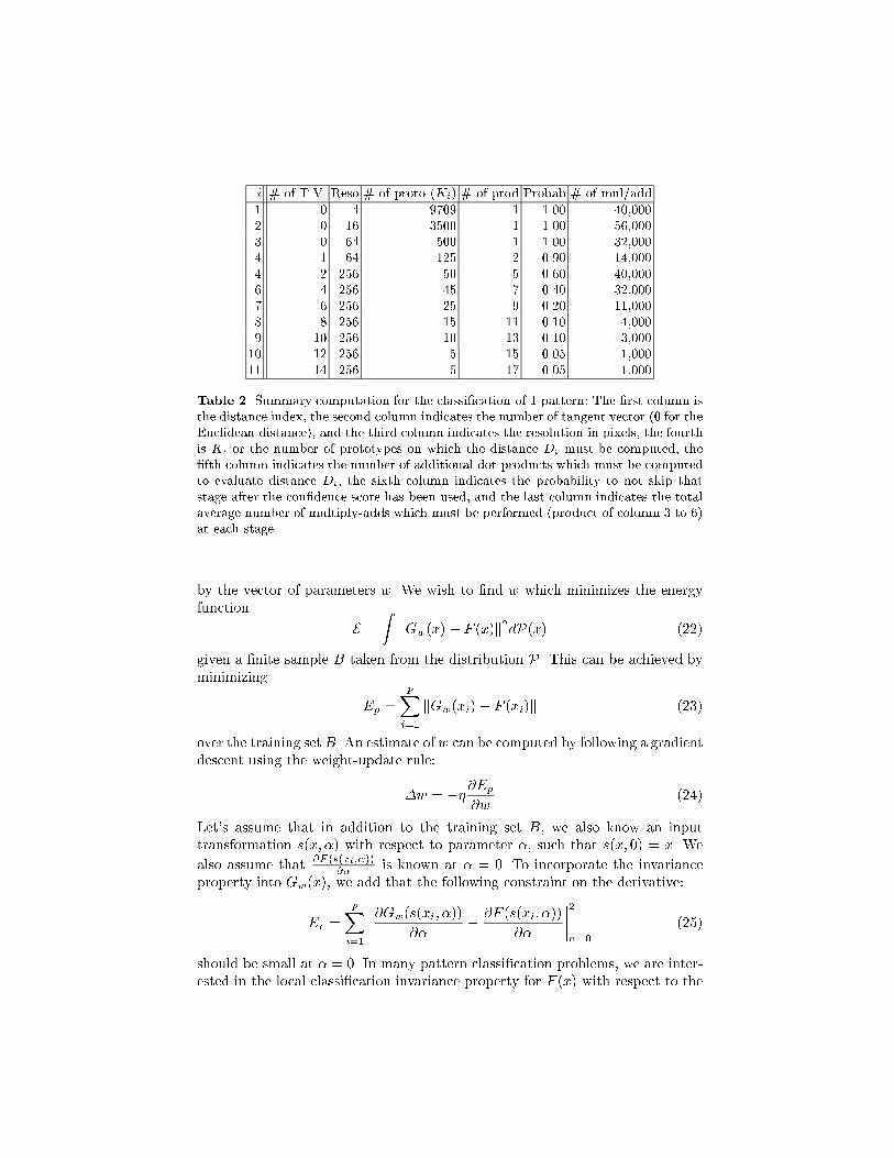
i # of T.V. Reso # of proto (Ki) # of prod Probab # of mul/add

1 0 4 9709 1 1.00 40,0002 0 16 3500 1 1.00 56,0003 0 64 500 1 1.00 32,0004 1 64 125 2 0.90 14,0004 2 256 50 5 0.60 40,0006 4 256 45 7 0.40 32,0007 6 256 25 9 0.20 11,0008 8 256 15 11 0.10 4,0009 10 256 10 13 0.10 3,00010 12 256 5 15 0.05 1,00011 14 256 5 17 0.05 1,000

Table 2. Summary computation for the classi�cation of 1 pattern: The �rst column isthe distance index, the second column indicates the number of tangent vector (0 for theEuclidean distance), and the third column indicates the resolution in pixels, the fourthis Ki or the number of prototypes on which the distance Di must be computed, the�fth column indicates the number of additional dot products which must be computedto evaluate distance Di, the sixth column indicates the probability to not skip thatstage after the con�dence score has been used, and the last column indicates the totalaverage number of multiply-adds which must be performed (product of column 3 to 6)at each stage.

by the vector of parameters w. We wish to �nd w which minimizes the energyfunction

E =

ZkGw(x) � F (x)k2dP(x) (22)

given a �nite sample B taken from the distribution P . This can be achieved byminimizing

Ep =

pXi=1

kGw(xi)� F (xi)k (23)

over the training set B. An estimate of w can be computed by following a gradientdescent using the weight-update rule:

�w = ��@Ep

@w(24)

Let's assume that in addition to the training set B, we also know an inputtransformation s(x; �) with respect to parameter �, such that s(x; 0) = x. We

also assume that @F (s(xi;�))@�

is known at � = 0. To incorporate the invarianceproperty into Gw(x), we add that the following constraint on the derivative:

Er =

pXi=1

����@Gw(s(xi; �))

@��@F (s(xi; �))

@�

����2

�=0

(25)

should be small at � = 0. In many pattern classi�cation problems, we are inter-ested in the local classi�cation invariance property for F (x) with respect to the

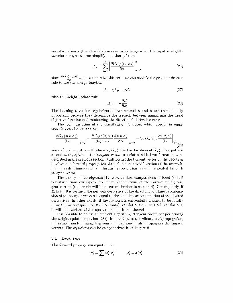
transformation s (the classi�cation does not change when the input is slightlytransformed), so we can simplify equation (25) to:

Er =

pXi=1

����@Gw(s(xi; �))

@�

����2

�=0

(26)

since @F (s(xi;�))@�

= 0. To minimize this term we can modify the gradient descentrule to use the energy function

E = �Ep + �Er (27)

with the weight update rule:

�w = �@E

@w(28)

The learning rates (or regularization parameters) � and � are tremendouslyimportant, because they determine the tradeo� between minimizing the usualobjective function and minimizing the directional derivative error.

The local variation of the classi�cation function, which appear in equa-tion (26) can be written as:

@Gw(s(x; �))

@�

�����=0

=@Gw(s(x; �))

@s(x; �)

@s(x; �)

@�

�����=0

= rxGw(x):@s(x; �)

@�

�����=0(29)

since s(x; �) = x if � = 0. where rxGw(x) is the Jacobian of Gw(x) for patternx, and @s(�; x)=@� is the tangent vector associated with transformation s asdescribed in the previous section. Multiplying the tangent vector by the Jacobianinvolves one forward propagation through a \linearized" version of the network.If � is multi-dimensional, the forward propagation must be repeated for eachtangent vector.

The theory of Lie algebras [11] ensures that compositions of local (small)transformations correspond to linear combinations of the corresponding tan-gent vectors (this result will be discussed further in section 4). Consequently, ifEr(x) = 0 is veri�ed, the network derivative in the direction of a linear combina-tion of the tangent vectors is equal to the same linear combination of the desiredderivatives. In other words, if the network is successfully trained to be locallyinvariant with respect to, say, horizontal translations and vertical translations,it will be invariant with respect to compositions thereof.

It is possible to devise an e�cient algorithm, \tangent prop", for performingthe weight update (equation (28)). It is analogous to ordinary backpropagation,but in addition to propagating neuron activations, it also propagates the tangentvectors. The equations can be easily derived from Figure 9.

3.1 Local rule

The forward propagation equation is:

ali =Xj

wlijx

l�1j xli = �(ali) (30)

Network Jacobian network

wl+1ki

�li �li

li li

bli

yli

bl�1j

xli

ali

xl�1j

�l�1j �l�1j

� �0

wl+1ki

wlij wl

ij

Fig. 9. Forward propagated variables (a; x; ; �), and backward propagated variables(b; y; �; ) in the regular network (roman symbols) and the Jacobian (linearized) net-work (greek symbols). Converging forks (in the direction in which the signal is traveling)are sums, diverging forks just duplicate the values.

Where � is a non linear di�erentiable function (typically a sigmoid). The forwardpropagation starts at the �rst layer (l = 1), with x0 being the input layer, andends at the output layer (l = L). Similarly, The tangent forward propagation(tangent prop) is de�ned by:

li =Xj

wlij�

l�1j �li = �0(ali)

li (31)

The tangent forward propagation starts at the �rst layer (l = 1), with �0 being

the tangent vector @s(x;�)@�

, and ends at the output layer (l = L). The tangentgradient backpropagation can be computed using the chain rule:

@E

@�li=Xk

@E

@ l+1k

@ l+1k

@�li

@E

@ li=@E

@�li

@�li@ li

(32)

�li =Xk

l+1k wl+1ki li = �li�0(ali) (33)

The tangent backward propagation starts at the output layer (l = L), with �L

being the network variation @Gw(s(x;�))@�

, and ends at the input layer. Similarly,

the gradient backpropagation is:

@E

@xli=Xk

@E

@al+1k

@al+1k

@xli

@E

@ali=@E

@xli

@xli@ali

+@E

@�li

@�li@ali

(34)

bli =Xk

yl+1k wl+1ki yli = bli�0(ali) + �i�

00(ali) li (35)

The standard backward propagation starts at the output layer (l = L), withxL = Gw(x

0) being the network output, and ends at the input layer. Finally,the weight update is:

�wlij = �

@E

@ali

@ali@wl

ij

�@E

@ li

@ li@wl

ij

(36)

�wlij = �ylixl�1j � li�

l�1j (37)

The computation requires one forward propagation and one backward propaga-tion per pattern and per tangent vector during training. After the network istrained, it is simply locally invariant with respect to the chosen transformation.The classi�cation computation is in all ways identical to a network which is nottrained for invariance (except for the weights which have di�erent values).

3.2 Results

Two experiments illustrate the advantages of tangent prop. The �rst experimentis a classi�cation task, using a small (linearly separable) set of 480 binarizedhandwritten digits. The training sets consist of 10, 20, 40, 80, 160 or 320 pat-terns, and the test set contains the remaining 160 patterns. The patterns aresmoothed using a Gaussian kernel with standard deviation of one half pixel. Foreach of the training set patterns, the tangent vectors for horizontal and verticaltranslation are computed. The network has two hidden layers with locally con-nected shared weights, and one output layer with 10 units (5194 connections,1060 free parameters) [19]. The generalization performance as a function of thetraining set size for traditional backprop and tangent prop are compared in Fig-ure 10. We have conducted additional experiments in which we implemented notonly translations but also rotations, expansions and hyperbolic deformations.This set of 6 generators is a basis for all linear transformations of coordinatesfor two dimensional images. It is straightforward to implement other generatorsincluding gray-level-shifting, \smooth" segmentation, local continuous coordi-nate transformations and independent image segment transformations.

The next experiment is designed to show that in applications where data ishighly correlated, tangent prop yields a large speed advantage. Since the dis-tortion model implies adding lots of highly correlated data, the advantage oftangent prop over the distortion model becomes clear.

The task is to approximate a function that has plateaus at three locations.We want to enforce local invariance near each of the training points (Figure 11,

0

10

20

30

40

50

60

Backprop

Tangent Prop

10 20 40 80 160 320

%Error onthe test set

Training set size

Fig. 10. Generalization performance curve as a function of the training set size for thetangent prop and the backprop algorithms

bottom). The network has one input unit, 20 hidden units and one output unit.Two strategies are possible: either generate a small set of training points coveringeach of the plateaus (open squares on Figure 11 bottom), or generate one trainingpoint for each plateau (closed squares), and enforce local invariance around them(by setting the desired derivative to 0). The training set of the former methodis used as a measure of performance for both methods. All parameters wereadjusted for approximately optimal performance in all cases. The learning curvesfor both models are shown in Figure 11 (top). Each sweep through the trainingset for tangent prop is a little faster since it requires only 6 forward propagations,while it requires 9 in the distortion model. As can be seen, stable performance isachieved after 1300 sweeps for the tangent prop, versus 8000 for the distortionmodel. The overall speedup is therefore about 10.

Tangent prop in this example can take advantage of a very large regulariza-tion term. The distortion model is at a disadvantage because the only parameterthat e�ectively controls the amount of regularization is the magnitude of the dis-tortions, and this cannot be increased to large values because the right answeris only invariant under small distortions.

3.3 How to make tangent prop work

Large network capacity: Not many experiments have been done with tangentpropagation. It is clear, however, that the invariance constraint is extremelystrong. If the network does not have enough capacity, it will not bene�t fromthe extra knowledge introduced by the invariance.

output output

Average NMSE vs ageAverage NMSE vs age

−1.5 −1 −0.5 0 0.5 1 1.5−1.5

−1

−0.5

0

0.5

1

1.5

−1.5 −1 −.5 0 .5 1 1.5−1.5

−1

−.5

0

.5

1

1.5

0 1000 2000 3000 4000 5000 6000 7000 8000 9000 100000

.1

.15

0 1000 2000 3000 4000 5000 6000 7000 8000 9000 100000

0.1

0.15

Tangent propDistortion model

Fig. 11. Comparison of the distortion model (left column) and tangent prop (rightcolumn). The top row gives the learning curves (error versus number of sweeps throughthe training set). The bottom row gives the �nal input-output function of the network;the dashed line is the result for unadorned back prop.

Interleaving of the tangent vectors: Since the tangent vectors introduceeven more correlation inside the training set, a substantial speed up can beobtained by alternating a regular forward and backward propagation with atangent forward and backward propagation (even if there are several tangentvectors, only one is used at each pattern). For instance, if there were 3 tangentvectors, the training sequence could be:

x1; t1(x1); x2; t2(x2); x3; t3(x3); x4; t1(x4); x5; t2(x5); : : : (38)

where xi means a forward and backward propagation for pattern i and tj(xi)means a tangent forward and backward propagation of tangent vector j of pat-tern i. With such interleaving, the learning converges faster than grouping all thetangent vectors together. Of course, this only makes sense with on-line learning.

4 Tangent Vectors

In this section, we consider the general paradigm for transformation invarianceand for the tangent vectors which have been used in the two previous sections.Before we introduce each transformation and their corresponding tangent vec-tors, a brief explanation is given of the theory behind the practice. There aretwo aspects to the problem. First it is possible to establish a formal connectionbetween groups of transformations of the input space (such as translation, rota-tion, etc. of <2) and their e�ect on a functional of that space (such as a mappingof <2 to <, which may represent an image, in continuous form). The theory ofLie groups and Lie algebra [6] allows us to do this. The second problem has to dowith coding. Computer images are �nite vectors of discrete variables. How cana theory which was developed for di�erentiable functional of <2 to < be appliedto these vectors?

We �rst give a brief explanation of the theorems of Lie groups and Lie al-gebras which are applicable to pattern recognition. Next, we explore solutionsto the coding problem. Finally some examples of transformation and coding aregiven for particular applications.

4.1 Lie groups and Lie algebras

Consider an input space I (the plane <2 for example) and a di�erentiable func-tion f which maps points of I to <.

f : X 2 B 7�! f(X) 2 < (39)

The function f(X) = f(x; y) can be interpreted as the continuous (de�ned forall points of <2) equivalent of the discrete computer image P [i; j].

Next, consider a family of transformations t�, parameterized by �, whichmaps bijectively a point of I to a point of I.

t� : X 2 I 7�! t�(X) 2 I (40)

We assume that t� is di�erentiable with respect to � and X , and that t0 is theidentity. For example t� could be the group of a�ne transformations of <2:

t� :

�xy

�7�!

�x+ �1x+ �2y + �5�3x+ y + �4y + �6

�with

����1 + �1 �2�3 1 + �4

���� 6= 0 (41)

It's a Lie group4 of 6 parameters. Another example is the group of direct isom-etry:

t� :

�xy

�7�!

�x cos � � y sin � + ax sin � + y cos � + b

�(42)

It's a Lie group of 3 parameters.

4 A Lie group is a group that is also a di�erentiable manifold such that the di�eren-tiable structure is compatible with the group structure.

We now consider the functional s(f; �), de�ned by

s(f; �) = f � t�1� (43)

This functional s, which takes another functional f as an argument, shouldremind the reader of Figure 2 where P , the discrete equivalent of f , is theargument of s.

The Lie algebra associated with the action of t� on f is the space generatedby the m local transformations L�i of f de�ned by:

Lai(f) =@s(f; �)

@�i

�����=0

(44)

We can now write the local approximation of s as:

s(f; �) = f + �1L�1(f) + �2L�2(f) + : : :+ �mL�m(f) + o(k�k2)(f) (45)

This equation is the continuous equivalent of equation (2) used in the introduc-tion.

The following example illustrates how L�i can be computed from t�. Let'sconsider the group of direct isometry de�ned in equation (42) (with parameter� = (�; a; b) as before, and X = (x; y)).

s(f; �)(X) = f((x� a) cos � + (y � b) sin �;�(x� a) sin � + (y � b) cos �) (46)

If we di�erentiate around � = (0; 0; 0) with respect to �, we obtain

@s(f; �)

@�(X) = y

@f

@x(x; y) + (�x)

@f

@y(x; y) (47)

that is

L� = y@

@x+ (�x)

@

@y(48)

The transformation La = � @@x

and Lb = � @@y

can be obtained in a similarfashion. All local transformation of the group can be written as

s(f; �) = f + �(y@f

@x+ (�x)

@f

@y)� a

@f

@x� b

@f

@y+ o(k�k2)(f) (49)

which corresponds to a linear combination of the 3 basic operators L�, La andLb

5. The property which is most important to us is that the 3 operators generatethe whole space of local transformations. The result of applying the operators toa function f , such as a 2D image for example, is the set of vectors which we havebeen calling \tangent vector" in the previous sections. Each point in the tangentspace correspond to a unique transformation and conversely any transformationof the Lie group (in the example all rotations of any angle and center togetherwith all translations) corresponds to a point in the tangent plane.

5 These operators are said to generate a Lie algebra, because on top of the additionand multiplication by a scalar, we can de�ned a special multiplication called \Liebracket" and de�ned by [L1; L2] = L1 �L2 �L2 �L1. In the above example we have[L� ; La] = Lb, [La; Lb] = 0, and [Lb; L�] = La.

4.2 Tangent vectors

The last problem which remains to be solved is the problem of coding. Computerimages, for instance, are coded as a �nite set of discrete (even binary) values.These are hardly the di�erentiable mappings of I to < which we have beenassuming in the previous subsection.

To solve this problem we introduce a smooth interpolating function C whichmaps the discrete vectors to continuous mapping of I to <. For example, if P isa image of n pixels, it can be mapped to a continuously valued function f over<2 by convolving it with a two dimensional Gaussian function g� of standarddeviation �. This is because g� is a di�erentiable mapping of <2 to <, and Pcan be interpreted as a sum of impulse functions. In the two dimensional casewe can write the new interpretation of P as:

P 0(x; y) =Xi;j

P [i][j]�(x� i)�(y � j) (50)

where P [i][j] denotes the �nite vector of discrete values, as stored in a computer.The result of the convolution is of course di�erentiable because it is a sum ofGaussian functions. The Gaussian mapping is given by:

C� : P 7�! f = P 0 � g� (51)

In the two dimensional case, the function f can be written as:

f(x; y) =Xi;j

P [i][j]g�(x� i; y � j) (52)

Other coding function C can be used, such as cubic spline or even bilinearinterpolation. Bilinear interpolation between the pixels yields a function f whichis di�erentiable almost everywhere. The fact that the derivatives have two valuesat the integer locations (because the bilinear interpolation is di�erent on bothside of each pixels) is not a problem in practice (just choose one of the twovalues).

The Gaussian mapping is preferred for two reasons: First, the smoothingparameter � can be used to control the locality of the invariance. This is becausewhen f is smoother, the local approximation of equation (45) is better (it is validfor large transformation). And second, when combined with the transformationoperator L, the derivative can be applied on the closed form of the Gaussianfunction. For instance, if the X-translation operator L = @

@xis applied to f =

P 0 � g�, the actual computation becomes:

LX(f) =@

@x(P 0 � g�) = P 0 �

@g�@x

(53)

because of the di�erentiation properties of convolution when the support is com-pact. This is easily done by convolving the original image with the X-derivative

= *

= *

= *

Fig. 12. Graphic illustration of the computation of f and two tangent vectors corre-sponding to Lx = @=@x (X-translation) and Lx = @=@y (Y-translation), from a binary

image I. The Gaussian function g(x; y) = exp(�x2+y2

2�2) has a standard deviation of

� = 0:9 in this example although its graphic representation (small images on the right)have been rescaled for clarity.

of the Gaussian function g� . This operation is illustrated in Figure 12. Similarly,the tangent vector for scaling can be computed with

LS(f) =

�x@

@x+ y

@

@y

�(I � g�) = x(I �

@g�@x

) + y(I �@g�@y

) (54)

This operation is illustrated in Figure 13.

4.3 Important transformations in image processing

This section summarizes how to compute the tangent vectors for image process-ing (in 2D). Each discrete image Ii is convolved with a Gaussian of standarddeviation g� to obtain a representation of the continuous image fi, according toequation:

fi = Ii � g�: (55)

The resulting image fi will be used in all the computations requiring Ii (exceptfor computing the tangent vector). For each image Ii, the tangent vectors arecomputed by applying the operators corresponding to the transformations ofinterest to the expression Ii � g�. The result, which can be precomputed, is animage which is the tangent vector. The following list contains some of the mostuseful tangent vectors:

=

=x

x

Fig. 13. Graphic illustration of the computation of the tangent vector Tu = DxSx +DySy (bottom image). In this example the displacement for each pixel is proportionalto the distance of the pixel to the center of the image (Dx(x; y) = x�x0 and Dy(x; y) =y�y0). The two multiplications (horizontal lines) as well as the addition (vertical rightcolumn) are done pixel to pixel.

X-translation: This transformation is useful when the classi�cation functionis know to be invariant with respect to the input transformation:

t� :

�xy

�7�!

�x+ �y

�(56)

The Lie operator is de�ned by:

LX =@

@x(57)

Y-translation: This transformation is useful when the classi�cation functionis know to be invariant with respect to the input transformation:

t� :

�xy

�7�!

�x

y + �

�(58)

The Lie operator is de�ned by:

LY =@

@y(59)

Rotation: This transformation is useful when the classi�cation function is knowto be invariant with respect to the input transformation:

t� :

�xy

�7�!

�x cos�� y sin�x sin�+ y cos�

�(60)

The Lie operator is de�ned by:

LR = y@

@x+ (�x)

@

@y(61)

Scaling: This transformation is useful when the classi�cation function is knowto be invariant with respect to the input transformation:

t� :

�xy

�7�!

�x+ �xy + �y

�(62)

The Lie operator is de�ned by:

LS = x@

@x+ y

@

@y(63)

Parallel hyperbolic transformation: This transformation is useful when theclassi�cation function is know to be invariant with respect to the input trans-formation:

t� :

�xy

�7�!

�x+ �xy � �y

�(64)

The Lie operator is de�ned by:

LS = x@

@x� y

@

@y(65)

Diagonal hyperbolic transformation: This transformation is useful whenthe classi�cation function is know to be invariant with respect to the in-put transformation:

t� :

�xy

�7�!

�x+ �yy + �x

�(66)

The Lie operator is de�ned by:

LS = y@

@x+ x

@

@y(67)

The resulting tangent vector is is the norm of the gradient of the image,which is very easy to compute.

Thickening: This transformation is useful when the classi�cation function isknow to be invariant with respect to variation of thickness. This is knowin morphology as dilation, or erosion. It is very useful in certain domain,such as handwritten character recognition because thickening and thinningare natural variations which correspond to the pressure applied on a pen, orto di�erent absorbtion property of the ink on the paper. A dilation (resp.erosion) can be de�ned as the operation of replacing each value f(x,y) bythe largest (resp. smallest) value of f(x0; y0) for (x0; y0) within a region of acertain shape, centered at (x; y). The region is called the structural element.We will assume that the structural element is a sphere of radius �. We de�ne

the thickening transformation as the function which takes the function f andgenerates the function f 0� de�ned by:

f 0�(X) = maxkrk<�

f(X + r) for � � 0 (68)

f 0�(X) = minkrk<��

f(X + r) for � < 0 (69)

The derivative of the thickening for � >= 0 can be written as:

lim��!0

f 0(X)� f(X)

�= lim

��!0

maxkrk<� f(X + r) � f(X)

�(70)

f(X) can be put within the max expression because it does not depend onkrk. Since k�k tends toward 0, we can write:

f(X + r)� f(X) = r:rf(X) +O(krk2) � r:rf(X) (71)

The maximum of

maxkrk<�

f(X + r)� f(X) = maxkrk<�

r:rf(X) (72)

is attained when r and rf(X) are co-linear, that is when

r = �rf(X)

krf(X)k(73)

assuming � > 0. It can easily be shown that this equation holds when � isnegative, because we then try to minimize equation (69). We therefore have:

lim��!0

f 0�(X)� f(X)

�= krf(X)k (74)

Which is the tangent vector of interest. Note that this is true for � positiveor negative. The tangent vectors for thickening and thinning are identical.Alternatively, we can use our computation of the displacement r and de�nethe following transformation of the input:

t�(f) :

�xy

�7�!

�x+ �rxy + �ry

�(75)

where

(rx; ry) = r = �rf(X)

krf(X)k(76)

This transformation of the input space is di�erent for each pattern f (wedo not have a Lie group of transformation, but the �eld structure generatedby the (pseudo Lie) operator is still useful. The operator used to �nd thetangent vector is de�ned by:

LT = krk (77)

which means that the tangent vector image is obtained by computing thenormalized gray level gradient of the image at each point (the gradient ateach point is normalized).

The last 5 transformation are depicted in Figure 14 with the tangent vector.The last operator corresponds to a thickening or thinning of the image. This un-usual transformation is extremely useful for handwritten character recognition.

Scaling Rotation Axis deformation Diagonaldeformation

Thicknessdeformation

Fig. 14. Illustration of 5 tangent vectors (top), with corresponding displacements (mid-dle) and transformation e�ects (bottom). The displacement Dx and Dy are representedin the form of vector �eld. It can be noted that the tangent vector for the thicknessdeformation (right column) correspond to the norm of the gradient of the gray levelimage.

5 Conclusion

The basic Tangent Distance algorithm is quite easy to understand and imple-ment. Even though hardly any preprocessing or learning is required, the perfor-mance is surprisingly good and compares well to the best competing algorithms.We believe that the main reason for this success is its ability to incorporate a

priori knowledge into the distance measure. The only algorithm which performedbetter than Tangent Distance on one of the three databases was boosting, whichhas the similar a priori knowledge about transformations built into it.

Many improvements are of course possible. First, a smart preprocessing canallow us to measure the Tangent Distance in a more appropriate \feature" space,instead of the original pixel space. In image classi�cation, for example, the fea-tures could be horizontal and vertical edges. This would most likely furtherimprove the performance6 The only requirement is that the preprocessing must

6 There may be an additional cost for computing the tangent vectors in the featurespace if the feature space is very complex.

be di�erentiable, so that the tangent vectors can be computed (propagated) intothe feature space.

Second, the Tangent Vectors and the prototypes can be learned from thetraining data, rather then chosen a priori. In applications such as speech, whereit is not clear to what transformation the classi�cation is invariant, the ability tolearn the Tangent Vector is a requirement. It is straightforward to modify algo-rithms such as LVQ (Learning Vector quantization) to use a tangent distance. Itis also straightforward to derive an batch [13] or on-line [23] algorithm to trainthe tangent vectors

Finally, many optimizations which are commonly used in distance based al-gorithms can be used as successfully with Tangent Distance to speed up com-putation. The multi-resolution approach have already been tried successfully[25]. Other methods like \multi-edit-condensing" [1, 30] and K-d tree [4] are alsopossible.

The main advantage of Tangent Distance is that it is a modi�cation of astandard distance measure to allow it to incorporate a priori knowledge that isspeci�c to your problem. Any algorithms based on a common distance measure(as it is often the case in classi�cation, vector quantization, predictions, etc...)can potentially bene�t from a more problem-speci�c distance. Many of this \dis-tance based" algorithms do not require any learning, which means that they canbe adapted instantly by just adding new patterns in the database. These addi-tions are leveraged by the a-priori knowledge put in the tangent distance.

The two drawbacks of tangent distance are its memory and computationalrequirements. The most computationally and memory e�cient algorithms gen-erally involve learning [20]. Fortunately, the concept of tangent vectors can alsobe used in learning. This is the basis for the tangent propagation algorithm.The concept is quite simple: instead of learning a classi�cation function fromexamples of its values, one can also use information about its derivatives. Thisinformation is provided by the tangent vectors. Unfortunately, not many exper-iments have been done in this direction. The two main problems with tangentpropagation are that the capacity of the learning machine has to be adjustedto incorporate the additional information pertinent to the tangent vectors, andthat training time must be increased. After training, the classi�cation time andcomplexity are unchanged, but the classi�er's performance is improved.

To a �rst approximation, using Tangent Distance or Tangent propagation islike having a much larger database. If the database was plenty large to beginwith, tangent distance or tangent propagation would not improve the perfor-mance. To a better approximation, tangent vector are like using a distortionmodel to magnify the size of the training set. In many cases, using tangent vec-tor will be preferable to collecting (and labeling!) vastly more training data,and preferable (especially for memory-based classi�ers) to dealing with all thedata generated by the distortion model. Tangent vectors provide a compact andpowerful representation of a-priori knowledge which can easily be integrated inthe most popular algorithms.

References

1. P. A.Devijver and J. Kittler. Pattern Recognition, A Statistical Approache. PrenticeHall, Englewood Cli�s, 1982.

2. Alfred V. Aho, John E. Hopcroft, and Je�rey D. Ullman. Data Structure andAlgorithms. Addison-Wesley, 1983.

3. L�eon Bottou and Vladimir N. Vapnik. Local learning algorithms. Neural Compu-tation, 4(6):888{900, 1992.

4. Alan J. Broder. Strategies for e�cient incremental nearest neighbor search. PatternRecognition, 23:171{178, 1990.

5. D. S. Broomhead and D. Lowe. Multivariable functional interpolation and adaptivenetworks. Complex Systems, 2:321{355, 1988.

6. Yvonne Choquet-Bruhat, Cecile DeWitt-Morette, and Dillard-Bleick. Analysis,Manifolds and Physics. North-Holland, Amsterdam, Oxford, New York, Tokyo,1982.

7. Corinna Cortes and Vladimir Vapnik. Support vector networks. Machine Learning,20:273{297, 1995.

8. Belur V. Dasarathy. Nearest Neighbor (NN) Norms: NN Pattern classi�cationTechniques. IEEE Computer Society Press, Los Alamitos, California, 1991.

9. Harris Drucker, Robert Schapire, and Patrice Y. Simard. Boosting performancein neural networks. International Journal of Pattern Recognition and Arti�cialIntelligence, 7, No. 4:705{719, 1993.

10. Keinosuke Fukunaga and Thomas E. Flick. An optimal global nearest neighbormetric. IEEE transactions on Pattern analysis and Machine Intelligence, 6, No.3:314{318, 1984.

11. R. Gilmore. Lie Groups, Lie Algebras and some of their Applications. Wiley, NewYork, 1974.

12. Trevor Hastie, Eyal Kishon, Malcolm Clark, and Jason Fan. A model for signatureveri�cation. Technical Report 11214-910715-07TM, AT&T Bell Laboratories, July1991.

13. Trevor Hastie and Patrice Y. Simard. Metrics and models for handwritten characterrecognition. Statistical Science, 13, 1998.

14. T. J. Hestie and R. J. Tibshirani. Generalized Linear Models. Chapman and Hall,London, 1990.

15. Geo�rey E. Hinton, Christopher K. I. Williams, and Michael D. Revow. Adap-tive elastic models for hand-printed character recognition. In Advances in NeuralInformation Processing Systems, pages 512{519. Morgan Kaufmann Publishers,1992.

16. A. E. Hoerl and R. W. Kennard. Ridge regression: Biased estimation for non-orthogonal problems. Technometrics, 12:55{67, 1970.

17. T. Kohonen. Self-organization and associative memory. In Springer Series inInformation Sciences, volume 8. Springer-Verlag, 1984.

18. Y. Le Cun, B. Boser, J. S. Denker, D. Henderson, R. E. Howard, W. Hubbard,and L. D. Jackel. Handwritten digit recognition with a back-propagation network.In David Touretzky, editor, Advances in Neural Information Processing Systems,volume 2, (Denver, 1989), 1990. Morgan Kaufman.

19. Y. LeCun. Generalization and network design strategies. In R. Pfeifer, Z. Schreter,F. Fogelman, and L. Steels, editors, Connectionism in Perspective, Zurich, Switzer-land, 1989. Elsevier. an extended version was published as a technical report ofthe University of Toronto.

20. Y. LeCun, L. D. Jackel, L. Bottou, C. Cortes, J. S. Denker, H. Drucker, I. Guyon,U. A. Muller, E. Sackinger, P. Simard, and V. Vapnik. Learning algorithms for clas-si�cation: A comparison on handwritten digit recognition. In J. H. Oh, C. Kwon,and S. Cho, editors, Neural Networks: The Statistical Mechanics Perspective, pages261{276. World Scienti�c, 1995.

21. E. Parzen. On estimation of a probability density function and mode. Ann. Math.Stat., 33:1065{1076, 1962.

22. W. H. Press, B. P. Flannery, Teukolsky S. A., and Vetterling W. T. NumericalRecipes. Cambridge University Press, Cambridge, 1988.

23. Holger Schwenk. The diabolo classi�er. Neural Computation, page in press, 1998.24. Robin Sibson. Studies in the robustness of multidimensional scaling: Procrustes

statistices. J. R. Statist. Soc., 40:234{238, 1978.25. Patrice Y. Simard. E�cient computation of complex distance metrics using hier-

archical �ltering. In Advances in Neural Information Processing Systems. MorganKaufmann Publishers, 1994.

26. Frank Sinden and Gordon Wilfong. On-line recognition of handwritten symbols.Technical Report 11228-910930-02IM, AT&T Bell Laboratories, June 1992.

27. V. N. Vapnik. Estimation of dependences based on empirical data. Springer Verlag,1982.

28. V. N. Vapnik and A. Ya. Chervonenkis. On the uniform convergence of rela-tive frequencies of events to their probabilities. Th. Prob. and its Applications,17(2):264{280, 1971.

29. Nuno Vasconcelos and Andrew Lippman. Multiresolution tangent distance fora�ne-invariant classi�cation. In Advances in Neural Information Processing Sys-tems, volume 10, pages 843{849. Morgan Kaufmann Publishers, 1998.

30. Jean Voisin and Pierre Devijver. An application of the multiedit-condensing tech-nique to the reference selection problem in a print recognition system. PatternRecogntion, 20 No 5:465{474, 1987.