Testing scale invariance in a two-dimensional Bose gas

HAL Id: tel-03591031https://tel.archives-ouvertes.fr/tel-03591031

Submitted on 28 Feb 2022

HAL is a multi-disciplinary open accessarchive for the deposit and dissemination of sci-entific research documents, whether they are pub-lished or not. The documents may come fromteaching and research institutions in France orabroad, or from public or private research centers.

L’archive ouverte pluridisciplinaire HAL, estdestinée au dépôt et à la diffusion de documentsscientifiques de niveau recherche, publiés ou non,émanant des établissements d’enseignement et derecherche français ou étrangers, des laboratoirespublics ou privés.

Testing scale invariance in a two-dimensional Bose gas :preparation and characterization of solitary waves

Brice Bakkali-Hassani

To cite this version:Brice Bakkali-Hassani. Testing scale invariance in a two-dimensional Bose gas : preparation andcharacterization of solitary waves. Quantum Gases [cond-mat.quant-gas]. Sorbonne Université, 2021.English. NNT : 2021SORUS375. tel-03591031

https://tel.archives-ouvertes.fr/tel-03591031

https://hal.archives-ouvertes.fr

Laboratoire Kastler Brossel College de France

These de doctorat de Sorbonne Universite

preparee par

Brice BAKKALI-HASSANI

Testing scale invariance in a two-dimensional Bose gas:

preparation and characterization of solitary waves

Soutenue le 10 decembre 2021 devant le jury compose de :

M. Gabriele FERRARI . . . . . . . . . . . . . . . . . . . . . . . . . . . . . . . . . . . . . . . . . . . . . . . . . . . RapporteurM. David GUERY-ODELIN . . . . . . . . . . . . . . . . . . . . . . . . . . . . . . . . . . . . . . . . . . . . . . RapporteurMme. Leticia TARRUELL . . . . . . . . . . . . . . . . . . . . . . . . . . . . . . . . . . . . . . . . . . . . . . ExaminatriceM. Xavier LEYRONAS . . . . . . . . . . . . . . . . . . . . . . . . . . . . . . . . . . . . . . . . . . . . . . . . . ExaminateurM. Jerome BEUGNON . . . . . . . . . . . . . . . . . . . . . . . . . . . . . . . . . . . . . . . . . . . . . . . . Membre inviteM. Jean DALIBARD . . . . . . . . . . . . . . . . . . . . . . . . . . . . . . . . . . . . . . . . . . . . . . Directeur de these

Travail realise au laboratoire Kastler Brossel, au sein du College de France.

3

Abstract

At a sufficiently large phase-space density, a Bose gas can be described by a macroscopicwave function subject to nonlinear dynamics. Degenerate Bose gases now constitute amajor platform in the study of self-trapped nonlinear fields known as solitons or solitarywaves. Up to now, most experimental observations of solitons have been restricted toone-dimensional situations, where they are generically stable. On the contrary, multi-dimensional solitary waves are more prone to instabilities and thus more challenging toobserve experimentally. In this thesis, we produce solitary waves in a two-dimensionalultracold bosonic system. After presenting our experimental setup, we demonstrate ourability to produce deterministically a Townes soliton, a celebrated solution of the nonlinearSchrodinger equation in two dimensions. Our novel approach is based on a two-componentmixture: starting from a uniform bath of atoms in a given internal state, we imprint thesoliton wave function using an optical transfer to another state. We show that the solitoncan exist with various sizes, a hallmark of the scale invariance present in the underlyingmodel. We then confirm the relation linking the soliton atom number to the interactionstrength. Our experimental observations are supported by further numerical and theoreti-cal considerations. These studies also allow us to go beyond the simplest model sustaininga Townes soliton, by considering effects beyond the mean-field description. Finally, wepropose a few experiments aimed at characterizing excited, moving, as well as collidingsolitons.

Resume

Lorsque la densite dans l’espace des phase d’un gaz de bosons identiques devient suff-isamment elevee, il peut alors etre decrit par une fonction d’onde macroscopique sujettea une dynamique non lineaire. Ces gaz quantiques sont aujourd’hui devenus des plate-formes incontournables dans l’etude des solitons, objets fondamentaux de la physique nonlineaire, aussi connus sous le nom d’ondes solitaires. Jusqu’a maintenant, l’essentiel desobservations experimentales de solitons a ete limite a des situations unidimensionnelles,ou les solitons sont stables naturellement. A l’inverse, les ondes solitaires de plus grandedimension sont generalement fragilisees par la presence d’instabilites dynamiques, ren-dant leur etude experimentale plus difficile. Dans cette these, nous produisons des ondessolitaires a partir d’un systeme de bosons bidimensionnel. Apres avoir presente notre dis-positif experimental, nous montrons comment preparer de facon deterministe un soliton deTownes – une solution remarquable de l’equation de Schrodinger non lineaire en dimensiondeux. Notre approche s’appuie sur l’utilisation d’un gaz a deux composantes : a partird’un echantillon uniforme d’atomes dans un etat interne donne, nous imprimons la fonc-tion d’onde du soliton grace a un transfert optique vers un autre etat. Nous verifions que lesoliton peut exister sous diverses tailles, confirmant ainsi l’invariance d’echelle du modelephysique sous-jacent. Nous confirmons egalement la relation liant le nombre d’atomescontenu dans le soliton et la force des interactions. Nos observations experimentales sontcorroborees par des etudes numeriques et theoriques. Par ailleurs, ces considerationsnous permettent d’etudier la physique au-dela du modele simple comportant un soliton deTownes, en considerant des effets allant au-dela du champ moyen. Finalement, nous pro-posons quelques experiences vouees a etudier les excitations, le mouvement et les collisionsde tels solitons.

Remerciements

C’est avec un immense plaisir et une emotion particuliere que je dedie ces premieres lignesa toutes les personnes qui m’ont, de pres ou de loin, permis de mener a bien cette longueaventure qu’est une these de doctorat.

Ces remerciements vont tout d’abord a mes directeurs de these, Jerome Beugnon etJean Dalibard. Jerome, tu m’as transmis l’essentiel de ce que je retire de ce travail derecherche. D’une aide indispensable au quotidien sur l’experience, tu m’as aussi permis detravailler a ma maniere, me laissant explorer des pistes qui ne paraissaient pas toujoursevidentes, m’aidant a ajuster la trajectoire lorsque necessaire. Merci pour tes conseils,ton ecoute et tes patientes relectures du manuscrit. Jean, tes enseignements – dont lalimpidite fait l’unanimite – ainsi que ta facon de guider les discussions sur la physiqueont profondement modifie ma vision des sciences. Merci pour ta disponibilite et pour tessuggestions qui ont fait murir de longues heures de reflexion, en particulier au moment oul’ecriture de ce manuscrit touche a sa fin. Merci egalement a Sylvain Nascimbene qui aenormement contribue aux travaux que je rapporte ici, par ses nombreux apports et sespropositions toujours eclairantes, lors de nos reunions et en dehors.

J’ai eu la chance d’integrer une equipe exceptionnelle des mon arrivee au laboratoire.Maintenant que ce doctorat touche a son terme, je percois d’autant mieux ce que cespersonnes m’ont apporte. Merci a Jean-Loup qui concluait l’ecriture de son manuscritau moment de mon stage, et avec qui j’ai fait mes premiers pas sur l’experience. Mercia Raphael qui, par ses conseils avises et son sens physique, a grandement contribue auxperformances de cette experience, depuis sa construction jusqu’a nos plus recents projets.Merci a Patricia qui m’a fait beneficier de sa grande experience, de sa rigueur et de sonenthousiasme pendant mes deux premieres annees de doctorat. Merci a Edouard pourses conseils et pour avoir partage son vaste savoir tout au long de ma these, jusqu’a sondepart. Enfin, merci a vous d’avoir amorce une serie d’experiences dont ce travail est leprolongement naturel.

Les generations de doctorant se succedant, ce fut bien vite a mon tour d’accueillir lesnouveaux-venus. Tout d’abord, un immense merci a Chloe avec qui j’ai eu la chance detravailler durant ces trois dernieres annees. Et pas des moindres ! Merci pour ton aide, tonsoutien, ces discussions et ces reflexions essentielles, tout ce sans quoi ce projet n’aurait puressembler a ce qui est retranscrit ci-apres. C’etait le moins que l’on puisse attendre d’unbinome qui fonctionne si bien. Merci mille fois de m’avoir confie Sohan, un petit chat untantinet turbulent mais si mignon a la fois. Merci egalement a Yiquan qui nous a apporteenormement durant les deux annees de son contrat post-doctoral. Un grand merci ensuitea Guillaume. Arrive en pleine crise sanitaire, tu as fait preuve d’une perseverance et d’unerigueur epatantes. Merci a Franco qui, tout juste debarque, est venu epauler Guillaumedans la construction d’une nouvelle experience. A terme, celle-ci remplacera le dispositifdont je rapporte ici les aventures. Merci a vous deux de rester sur tous les fronts, vous

5

6

montrant chaque fois curieux de comprendre ce que nous mijotons a cote. Il ne fait pasde doutes que l’equipe Rubidium a encore de tres beaux jours devant elle.

La vie de laboratoire ne serait pas la meme sans compter toutes les personnes quihabitent ou ont habite le deuxieme etage du batiment E. Merci a celles et ceux qui ontrendu ces annees si enrichissantes, aussi bien humainement que scientifiquement, aussi bienautour d’un cafe, d’un croissant, d’un cake banane-Nutella, que d’une pinte de biere. Mercia Chayma, Raphael, Thomas, Manel, Nicolas, An, Bertrand, Merlin, Alexis, Alexandre,Sebastien, Tanish, Remy, Aurelien, Julien, Jean-Baptiste, Quentin, Tristan, Sarah, Virgin.Merci a Raphael Lopes et Alexei Ourjoumtsev qui ont toujours ete disponibles lorsque jeles sollicitais. Merci a Carmen Toderasc et a toute l’equipe administrative du LKB pourleur aide si precieuse. Merci egalement aux amis du rez-de-chaussee, Paul, Lea, Remy,Andrea, Brice, Rodrigo, et a toutes celles et ceux que j’ai eu la chance de cotoyer auCollege de France. Merci enfin a Nicolas Treps, mon parain pendant ces trois annees,pour son ecoute ainsi que ses conseils.

Ce travail n’aurait pas ete ce qu’il est sans le soutien inconditionnel de mes proches,de mes amis et de ma famille. Merci a mes parents d’avoir ete toujours presents et pleinsd’enthousiame. Un grand merci a mon frere et a ma soeur pour qui l’aventure du doctoratn’est pas si etrangere. Merci a mes comparses sans qui ces annees de these aurait etenettement moins marrantes, je pense bien evidemment a Bruno et a Tristan. D’ou qu’ilslisent ces lignes, je leur dis simplement bonjour. Merci a Francois qui saura, probablementmieux que moi, expliquer le contenu de cette these, le tout en musique. Merci a Elisa quia rendu cette derniere annee de doctorat si merveilleuse, et qui m’a accompagne dans lesjours les plus difficiles de la redaction de ce manuscrit. Merci enfin a toutes celles et ceuxqui ont ete la durant ces annees, Marius, Maxime, Simon, Ayman, Lisa, Lina, Alice, Elise,Serena, Pierre, Gaspard, Damien, Francesca, Artiom, Radu-Alexandru, Perrine, Sarah,tous les voisins du 142 rue d’Avron et toute l’equipe du centre Emmaus Pyrenees.

Contents

Introduction 11

1 Production of planar Bose gases 17

1.1 Experimental sequence . . . . . . . . . . . . . . . . . . . . . . . . . . . . . . 17

1.1.1 Preliminary steps . . . . . . . . . . . . . . . . . . . . . . . . . . . . . 18

1.1.2 A tunable horizontal confinement . . . . . . . . . . . . . . . . . . . . 22

1.1.3 Some calibrations . . . . . . . . . . . . . . . . . . . . . . . . . . . . . 26

1.2 Preparation of binary mixtures . . . . . . . . . . . . . . . . . . . . . . . . . 29

1.2.1 Internal degrees of freedom . . . . . . . . . . . . . . . . . . . . . . . 29

1.2.2 Magnetic dipole-dipole interactions . . . . . . . . . . . . . . . . . . . 33

1.3 Conclusion . . . . . . . . . . . . . . . . . . . . . . . . . . . . . . . . . . . . 36

2 Description of a two-dimensional Bose gas 37

2.1 Description at zero temperature . . . . . . . . . . . . . . . . . . . . . . . . . 37

2.1.1 The nonlinear Schrodinger equation . . . . . . . . . . . . . . . . . . 37

2.1.2 Ground state and dynamics . . . . . . . . . . . . . . . . . . . . . . . 40

2.1.3 Symmetries in two dimensions . . . . . . . . . . . . . . . . . . . . . 43

2.2 Description at finite temperature . . . . . . . . . . . . . . . . . . . . . . . . 46

2.2.1 Classical field formalism . . . . . . . . . . . . . . . . . . . . . . . . . 47

2.2.2 Description at low temperature . . . . . . . . . . . . . . . . . . . . . 48

2.2.3 Berezinskii-Kosterlitz-Thouless transition . . . . . . . . . . . . . . . 50

2.3 Conclusion . . . . . . . . . . . . . . . . . . . . . . . . . . . . . . . . . . . . 52

3 Physics of Townes soliton 53

3.1 Solitons of the nonlinear Schrodinger equation . . . . . . . . . . . . . . . . . 53

3.1.1 Solitons in one dimension . . . . . . . . . . . . . . . . . . . . . . . . 54

3.1.2 Multidimensional solitons . . . . . . . . . . . . . . . . . . . . . . . . 58

3.2 Properties of the Townes soliton . . . . . . . . . . . . . . . . . . . . . . . . 62

3.2.1 Stationary states of the 2D NLSE . . . . . . . . . . . . . . . . . . . 62

3.2.2 Stability of the Townes soliton . . . . . . . . . . . . . . . . . . . . . 66

3.3 Wave-packet collapse . . . . . . . . . . . . . . . . . . . . . . . . . . . . . . . 68

3.3.1 Conditions for collapse . . . . . . . . . . . . . . . . . . . . . . . . . . 68

3.3.2 Collapse dynamics . . . . . . . . . . . . . . . . . . . . . . . . . . . . 70

3.4 A recent experiment . . . . . . . . . . . . . . . . . . . . . . . . . . . . . . . 71

3.4.1 Quench of a 2D Bose gas . . . . . . . . . . . . . . . . . . . . . . . . 71

3.4.2 Modulational instability . . . . . . . . . . . . . . . . . . . . . . . . . 71

3.5 Conclusion . . . . . . . . . . . . . . . . . . . . . . . . . . . . . . . . . . . . 73

7

8 CONTENTS

4 Realization of a Townes soliton 75

4.1 Effective one-component dynamics . . . . . . . . . . . . . . . . . . . . . . . 75

4.1.1 Weak depletion regime . . . . . . . . . . . . . . . . . . . . . . . . . . 75

4.1.2 Preparation and detection . . . . . . . . . . . . . . . . . . . . . . . . 78

4.1.3 An example dynamics . . . . . . . . . . . . . . . . . . . . . . . . . . 81

4.2 Dynamics of a Townes profile . . . . . . . . . . . . . . . . . . . . . . . . . . 82

4.2.1 Various atom numbers . . . . . . . . . . . . . . . . . . . . . . . . . . 83

4.2.2 Check of scale invariance . . . . . . . . . . . . . . . . . . . . . . . . 86

4.2.3 Finite-depletion regime . . . . . . . . . . . . . . . . . . . . . . . . . 88

4.3 Conclusion . . . . . . . . . . . . . . . . . . . . . . . . . . . . . . . . . . . . 89

5 Single-component description of a binary mixture 91

5.1 Two-component description . . . . . . . . . . . . . . . . . . . . . . . . . . . 91

5.1.1 An immiscible mixture . . . . . . . . . . . . . . . . . . . . . . . . . . 91

5.1.2 Spin bubbles . . . . . . . . . . . . . . . . . . . . . . . . . . . . . . . 94

5.2 Effective one-component description . . . . . . . . . . . . . . . . . . . . . . 98

5.2.1 Turning the coupled NLSEs into a single one . . . . . . . . . . . . . 98

5.2.2 A microscopic point-of-view . . . . . . . . . . . . . . . . . . . . . . . 102

5.3 Beyond the nonlinear Schrodinger equation . . . . . . . . . . . . . . . . . . 104

5.3.1 Polaron physics . . . . . . . . . . . . . . . . . . . . . . . . . . . . . . 104

5.3.2 The influence of finite temperature . . . . . . . . . . . . . . . . . . . 104

5.3.3 Beyond mean-field effects . . . . . . . . . . . . . . . . . . . . . . . . 105

5.4 Conclusion . . . . . . . . . . . . . . . . . . . . . . . . . . . . . . . . . . . . 107

6 Perspectives on spin bubbles dynamics 109

6.1 Stability and elementary excitations . . . . . . . . . . . . . . . . . . . . . . 109

6.1.1 Methods . . . . . . . . . . . . . . . . . . . . . . . . . . . . . . . . . . 110

6.1.2 Weak depletion regime . . . . . . . . . . . . . . . . . . . . . . . . . . 111

6.1.3 Surface modes . . . . . . . . . . . . . . . . . . . . . . . . . . . . . . 113

6.1.4 The experimental point-of-view . . . . . . . . . . . . . . . . . . . . . 115

6.2 Collisions of Townes solitons . . . . . . . . . . . . . . . . . . . . . . . . . . . 116

6.2.1 Collisions under the cubic NLSE . . . . . . . . . . . . . . . . . . . . 116

6.2.2 Extension to a binary mixture . . . . . . . . . . . . . . . . . . . . . 119

6.3 Conclusion . . . . . . . . . . . . . . . . . . . . . . . . . . . . . . . . . . . . 120

Summary and outlook 121

A Elementary excitations of the Townes soliton 123

A.1 Continuous symmetries . . . . . . . . . . . . . . . . . . . . . . . . . . . . . 123

A.2 Stability analysis . . . . . . . . . . . . . . . . . . . . . . . . . . . . . . . . . 125

A.3 Neutral modes and symmetries . . . . . . . . . . . . . . . . . . . . . . . . . 126

B Variational method 129

C Anisotropic contribution of MDDI 131

D Perturbative expansions for data analysis 135

D.1 Dynamics of Townes profiles . . . . . . . . . . . . . . . . . . . . . . . . . . . 135

D.2 Dynamics of Gaussian profiles . . . . . . . . . . . . . . . . . . . . . . . . . . 136

CONTENTS 9

E Numerical recipes for the 2D NLSE 137E.1 Resolution in 2D . . . . . . . . . . . . . . . . . . . . . . . . . . . . . . . . . 137E.2 Using radial coordinates . . . . . . . . . . . . . . . . . . . . . . . . . . . . . 140

F Induced interactions 143F.1 A single impurity . . . . . . . . . . . . . . . . . . . . . . . . . . . . . . . . . 143F.2 The effective potential . . . . . . . . . . . . . . . . . . . . . . . . . . . . . . 146

G Elementary excitations of spin bubbles 149

H Publications 153

Bibliography 189

10 CONTENTS

Introduction

The wave function is a fundamental concept in quantum physics. This function associatesa complex-valued probability amplitude to each possible configuration of a physical system.In non-relativistic quantum mechanics, the state of any isolated system of particles can bedescribed in this manner. Because its evolution is described by a linear wave equation –the Schrodinger equation – the wave function behaves essentially like other waves do, beit sound or light. In particular, this wave-like description brings the possibility to observeinterference phenomena, which arise when multiple waves associated to the same fieldoverlap. The duality between a wave-like and a corpuscular behavior is itself at the origin ofseveral difficulties in the interpretation of quantum mechanics. Experimentally, quantuminterference can now be observed using mesoscopic systems, such as large molecules forinstance [1–3]. Nonetheless, the description of most macroscopic systems in terms of awave function is out of reach. Indeed, the number of arguments of this function then scaleslike the number of particles. Moreover, interactions between particles generically lead tocomplicated correlations that cannot be disentangled. As a corollary, the observation ofinterference phenomena is usually unrealistic for such systems.

For a many-body system, there are specific situations which allow a description withmuch less degrees of freedom. For instance, if an assembly of indistinguishable particlesoccupies the same state, then it is sufficient to use a single-particle wave function – themacroscopic wave function – to describe the whole system. When the number of particlesis so large that one can neglect its discrete nature, the problem can be reduced to aclassical field theory for this macroscopic wave function. In such cases, the correspondingstate bears a well-defined phase and can lead to interference phenomena. This coherentfield has thus a lot in common with the electromagnetic field emitted by a laser source.This reasoning can also be extended to a situation where only a few single-particle statesare massively populated. In this case, the macroscopic state will be described by a fieldinvolving the same number of components as there are relevant states.

Which conditions can lead to such a behavior? First of all, the particles should bebosons since they can occupy the same quantum state. Remarkably, the above situa-tion appears as a direct consequence of the phenomenon of Bose-Einstein condensation,initially predicted for an ideal system of massive bosons [4]. Below a certain critical tem-perature, a macroscopic fraction of the particles is expected to accumulate in the state oflowest energy. This transition is thus a manifestation of the gregarious nature of bosons.A description in terms of a classical field has been fruitful in the case of superfluid Helium4, which was realized to exhibit quantum mechanical properties on a large scale soon afterits discovery [5]. This also applies to the Ginzburg-Landau theory of superconductivity [6]for which the notion of a common state is meaningful only for pairs of electrons, the lat-ter being fermions. In both situations, this classical field description is supported by theobservation of coherent phenomena, such as Josephson oscillations or quantized vortices.

11

12 INTRODUCTION

Moreover, there is a deep connection between these two behaviors and the phenomenon ofBose-Einstein condensation. However, interactions are never rigorously absent for massiveparticles and, in these situations, the use of a macroscopic wave function is mostly phe-nomenological. Indeed, a rigorous derivation of a classical field theory from microscopicprinciples is hindered by the presence of strong interactions and the induced correlations.

Experimentally, ultracold quantum gases provide an important realization of a weakly-interacting system. Since the first demonstration of Bose-Einstein condensation in 1995[7, 8], these dilute, defect-free, isolated and fully tunable systems have become a majortool in the study of many-body quantum phenomena. In an early and spectacular exper-iment, two separated condensates were made overlapping and displayed an interferencepattern [9]. This – and many other experiments – confirmed the wave-like properties ofultracold bosonic systems, often referred to as coherent matter-waves. On the theoreti-cal point-of-view, the macroscopic state of the system can be understood using a single-particle nonlinear wave equation for the macroscopic wave function, the so-called nonlinearSchrodinger equation (NLSE). In the context of superfluid systems, this equation is alsoknown as the Gross-Pitaevskii equation. Most developments presented in this thesis willrely on this model. In the weakly-interacting regime, the nonlinear term can be obtaineddirectly by treating all interactions in a mean-field picture. Although the full quantumproblem is itself linear with respect to the many-body wave function, the appearance ofan effective nonlinearity is the price to pay for this considerable simplification.

Since they can be described using a nonlinear wave equation, quantum gases soonbecame a novel platform for the study of nonlinear phenomena. While the importance oflinear physics does not need to be debated, nonlinear physical phenomena have becomea central and transverse research field over the second half of the twentieth century. Inparticular, physicists have realized that nonlinear wave equations, although more difficultto grasp and to analyze mathematically, could lead in general to much richer behaviors.Historically, nonlinear physics have first become a prominent research axis in the contextof hydrodynamics. Indeed, the Navier-Stokes equations on its own can yield a multitudeof nonlinear behaviors such as various types of instabilities [10].

Solitons are probably some of the most important and fascinating objects in nonlinearphysics. In mathematical terms, solitons can be defined as stationary solutions of nonlinearwave equations. They typically arise from the compensation of a linear dispersion effectby a nonlinear contraction mechanism. Solitons were first discovered in the context ofhydrodynamics, for one-dimensional (1D) problems. In 1845, J. S. Russell [11] described asolitary elevation of water propagating in a narrow channel. Importantly, his observationscould not be interpreted using a linear wave equation. At that time, the impact of thisdiscovery was already undeniable at the theoretical level. Yet, the generality and the scopeof the concept of solitons could not be properly appreciated, both on the theoretical andthe experimental side. Following the work of Zabusky & Kruskal [12] in 1965, solitonswere shown to be extremely general and stable solutions for some 1D problems. Moregenerally, solitons are encountered in a broad range of physical settings, including nonlinearphotonics, hydrodynamics, superconductors, polymers, plasmas, and even high-energyphysics [13].

In dimension larger than one, the creation, the manipulation and the observation of self-bound fields is a central challenge [14]. Indeed, there exists a great variety of such states,in particular because these can feature a nontrivial topology. Moreover, the dynamics andthe interactions between such objects bring an even richer phenomenology [15]. In parallel,

13

the introduction of multiple components in the field degrees of freedom can also lead tonew behaviors and can yield composite solitons. Unfortunately, the solitons present in themost simple NLSE models are generically unstable with respect to small perturbations, aproperty less present in 1D systems. To circumvent this issue, numerous strategies havebeen proposed theoretically to protect these states against instabilities, and few of theseexperiments have been implemented.

Let us discuss specifically the case of nonlinear optics. Soon after the invention of lasersin 1960, it was realized that the propagation of coherent and intense light beams throughmatter was significantly affected by nonlinear (Kerr) effects. Moreover, in a stationarysituation well captured by the paraxial approximation, this behavior can be describedusing the NLSE by replacing the time variable by the distance on the propagation axis.This culminated with the first observations of nonlinear self-trapping of light [16–19], andsoliton propagation in optical settings [20, 21]. Intriguingly, it turns out that light andmatter – which are fundamentally of very different nature – can be described in a unifiedframework under specific conditions.

In this thesis, we will be interested in the celebrated Townes soliton. This solitonis a localized solution of the 2D NLSE with a cubic nonlinearity. More precisely, it isthe unique real, nodeless, and axially symmetric solution of the 2D NLSE. The Townessoliton was first predicted by Chiao et al. [17] and Talanov [18] in the context of self-trapping of intense laser beams in nonlinear media. This soliton bears some peculiarproperties inherited from the 2D NLSE. For instance, its L2-norm is fixed by the strengthof the nonlinearity. Furthermore, it can be formed with any size, a hallmark of the scaleinvariance of the 2D NLSE. However, the Townes soliton is unstable as small deviationsaway from equilibrium can lead to the collapse of the field. For all these reasons, the questfor this soliton has triggered a myriad of experimental works in nonlinear optical settings.

The toolbox of the cold-atom physicist is particularly well adapted to the preparationand the study of multidimensional fields, especially when complex state engineering isrequired. On the one hand, the availability of high-resolution optical systems allows thein-situ observation of quantum gases with unprecedented accuracy. On the other hand,a great variety of initial states and Hamiltonians can now be tailored. For instance, thegeometry of these systems can be controlled using a great variety of optical potentials.This has allowed the observation of dark and bright solitons in quasi-1D geometry inpioneering experiments [22–24]. Furthermore, spatial light modulators now allow theproduction of ever-more complex light-field configurations. Such techniques can be usedto design optical box potentials [25] or to imprint specific phase profiles on the atomicwave function. In addition, atomic species naturally come with an internal structurewhich allows the exploration of multi-component or spinor physics [26]. This was recentlyillustrated by the realization of magnetic solitons in two-component [27] or spin-1 Bose-Einstein condensates [28].

Interestingly, quantum gases also offer the possibility to go beyond a description interms of a classical field. In particular, the use of Feshbach resonances [29] has allowedto explore strongly correlated phases of matter, while staying in the dilute regime wherea theoretical treatment is still conceivable. Is it possible to observe effects beyond themean-field description, without leaving the regime of weak interactions? In 2015, Petrov[30] positively answered this question by introducing the concept of quantum droplets.Experimentally, such droplets have now been realized using either binary mixtures ofquantum gases described by short-range interactions [31,32] and single-component systems

14 INTRODUCTION

of highly-magnetic atoms where dipole-dipole interactions play a significant role [33, 34].In both cases, the interactions – treated at the mean-field level – are set to be weaklyattractive, yielding an unstable situation a priori. The inclusion of quantum fluctuations– going beyond the mean-field description – then provides a repulsive effect with a differentscaling in density which can stabilize the system. Eventually, the balance between thesetwo mechanisms defines an equilibrium density. A large system would feature a flat-topdensity profile over a large region, similarly to an incompressible fluid. These constitutean important realization of stabilized multidimensional fields.

Quantum droplets bear strong analogies with other systems encountered in condensedmatter physics, such as Helium droplets [35–37]. In this last case, however, the densitiesand the effect of interactions make the system not amenable to a rigorous theoreticaltreatment. The discovery of dilute quantum droplets has thus opened new directions togain insight on quantum liquids. Furthermore, these systems also allow to study exoticphases of matter such as supersolids, which were predicted in 1970 by Leggett in thecontext of solid Helium [38]. According to the current definition, a supersolid shouldpresent both superfluid properties and an interaction-induced periodic density modulation.Interestingly, the NLSE with a well-chosen nonlocal nonlinearity can support a groundstate with supersolid properties [39]. Emergent platforms having demonstrated signaturesof supersolidity include dipolar quantum gases [40–42], systems interacting strongly withoptical cavities [43], spin-orbit-coupled BECs [44].

In this manuscript, I present our recent realization of a Townes soliton using a two-component planar Bose gas [45]. Our experimental apparatus allows us to prepare coldbosonic samples confined in two dimensions (2D), with a versatile potential in the hor-izontal plane. At zero temperature, one can faithfully use a description in terms of aclassical field satisfying the 2D NLSE. Since interactions in the system are all repulsive,our situation seems a priori incompatible with the attractive interactions required to ob-serve a Townes soliton. We developed a novel approach using a two-component system.In the case where one component is in a strong minority, one obtains effectively attractiveinteractions between the atoms in this component. In contrast with other recent studies of2D solitary waves emerging from a dynamical instability [46,47], we deterministically pre-pared a Townes soliton using an optical transfer. Finally, we also draw fruitful analogiesbetween our system and the behavior of quantum droplets.

I will now detail the content of this thesis.

– In Chapter 1, I describe the experimental platform which allows us to prepareplanar samples of Rubidium 87. In particular, I discuss the techniques used fortailoring controllable optical fields, as reported in [48]. This is crucial to preparebinary systems with arbitrary spin distributions.

– In Chapter 2, I provide some theoretical tools to describe the weakly-interacting2D Bose gas. I also justify the use of the NLSE for studying this system even at low(but finite) temperature.

– In Chapter 3, I discuss the existence and the properties of solitons, focusing on thesingle-component NLSE with attractive interactions. In particular, I introduce thecelebrated Townes soliton and discuss its main features.

– In Chapter 4, I present our main experimental results concerning the determinis-tic preparation and the characterization of Townes solitons using a two-component

15

planar Bose gas. Starting from a uniform bath of atoms in a given state, our proto-col consists in imprinting the wave function of the Townes soliton using an opticaltransfer to another state. Throughout this manuscript, this novel composite systemwill be called a spin bubble.

– In Chapter 5, I justifiy the use of a single-component attractive NLSE for inter-preting the results of Chapter 4, even though the system is made of two componentswith only-repulsive interactions. This mapping is rooted in the immiscible characterof the binary mixture.

– In Chapter 6, I propose a few directions for future characterizations of spin bub-bles. More precisely, I determine the excitation spectrum of spin bubbles in variousregimes. I also investigate the outcome of binary collisions of Townes solitons.

– In the various appendices gathered at the end of the manuscript, I complement someof our results and derive some others step-by-step.

During my thesis, I had the opportunity to work on several other projects using thisexperimental setup. Most of these results not being detailed in the manuscript, I nowdedicate a few lines to mention them. A list of the four corresponding publications can befound in Appendix H. The weakly-interacting 2D Bose gas has specific properties, both atequilibrium and from a dynamical point-of-view. In [49], we related far-from-equilibriumdynamics of distinct initial systems linked by scaling transformations. We also reportedthe discovery of breathing solutions of the nonlinear dynamics. The emergence of a su-perfluid phase in 2D at low temperature is described by a peculiar phase transition, theso-called Berezinskii-Kosterlitz-Thouless phase transition. A noteworthy signature of thistransition shows up in the first-order correlation function of the system, which quanti-fies the spatial coherence of the atomic field. This function decays exponentially fast inthe normal phase, whereas it is expected to show a power-law behavior in the superfluidphase. A determination of this correlation function using matter-wave experiments hasbeen reported in the thesis of Raphael Saint-Jalm [50]. During this last year, we developeda spectroscopic method analogous to Ramsey interferometry for our many-body system.Using this method, we could measure the so-called Tan’s contact accross the BKT transi-tion [51]. We could also reveal the subtle effect of magnetic dipole-dipole interactions ina 2D geometry [52]. Finally, our exploration of immiscible binary mixtures started withthe study of the demixion instability [53].

16 INTRODUCTION

Chapter 1

Production of planar Bose gases

This thesis explores some aspects specific to quantum planar systems. For a two-dimensional(2D) system of atoms with mass m, density n and temperature T , the importance of quan-tum statistics on collective properties is quantified by the so-called phase-space density

D = nλ2th, (1.1)

which compares the inter-particle distance ∼ n−1/2 to the thermal wavelength λth =√2π~2/mkBT . At standard temperatures, λth gives the typical extension of individual

wave packets. A large system reaches the regime of quantum degeneracy when this wave-length gets of the order of to the inter-particle distance, or equivalently when D becomes oforder unity. As a celebrated example, preparing an assembly of bosons at a large phase-space density in 3D may allow one to observe Bose-Einstein condensation [4], i.e. themacroscopic accumulation of particles in the state of lowest energy. Quantum gases thusoffer a unique access to exotic states of matter [54]. However, the preparation of suchsystems requires the control of both the internal and the external degrees of freedom ofindividual atoms.

In this chapter, we present the setup used throughout this thesis to produce 2D degen-erate samples of gaseous Rubidium 87 (87Rb), a bosonic isotope with one valence electronand a nuclear spin I = 3/2 [55]. While many species can now be brought to quantumdegeneracy, atomic vapors of 87Rb keep the advantage of being easily cooled and manip-ulated. Since most of the current setup was built before my arrival in the group, we referthe reader to the previous Master and PhD theses [50,53,56–58] for detailed characteriza-tions. As we show in Sec 1.1, we are able to create a single slab of atoms in the quasi-2Dregime, with a fully programmable in-plane geometry. The central topic of this thesis isthe study of solitons using binary mixtures. In Sec 1.2, we show how to manipulate theinternal degree of freedom of the atoms for the preparation of two-component planar Bosegases.

1.1 Experimental sequence

We first summarize the ingredients for the preparation of 2D systems with an arbitrarygeometry in the horizontal plane. The preliminary steps for all our experiments are pre-sented in Subsec 1.1.1, while Subsec 1.1.2 is devoted to the description of our horizontalconfinement. Finally, some calibrations needed to characterize the system are detailed inSubsec 1.1.3.

17

18 CHAPTER 1. PRODUCTION OF PLANAR BOSE GASES

Fine

structure

(n = 5)

2S1/2

2P1/2

2P3/2

D1

λ1=

795nm D2

λ2=

780nm

Hyperfine

structure

(I = 3/2)

F = 1

F = 2

ν ' 6.8 GHz

F ′ = 3

F ′ = 2

F ′ = 1

F ′ = 0

Zeeman

sublevels

(B 6= 0)

mF = 1

mF = 0

mF = −1

mF = −2

mF = −1

mF = 0

mF = 1

mF = 2

ν/B =

0.7 MHz/G

Light cooling2D & 3D MOT+ Molasses

7 s

N ∼ 109 T ∼ 250 µK

Magnetic trap+ Radio-frequency

Evaporation

14 s

N ∼ 2 · 107 T ∼ 20 µK

Hybrid trapCrossed dipoles & ∇B+ Optical evaporation

4 s

N ∼ 1 · 106 T . 200 nK

Green boxDMD & Accordion

+ Optical evaporation

1 s

N ∼ 1 · 105 T . 50 nK

(a) (b)

Figure 1.1: (a) Internal structure of 87Rb. We depicted only levels relevant for the ex-periments. All states have a principal quantum number n = 5 for the valence electron.Light on the D2 line is slightly red-detuned with respect to the (F = 2→ F ′ = 3) cyclingtransition, used for laser-cooling. The hyperfine splitting in the electronic ground statemanifold lies in the micro-wave domain, and the degeneracy between the various Zeemansublevels is lifted in the presence of a magnetic field B. The two states figured in red,|F = 1,mF = 0〉 ≡ |1〉 and |F = 2,mF = 0〉 ≡ |2〉, are the protagonists of our experimen-tal findings. (b) Time-line of the experimental sequence showing the duration of the maintime-steps. The resulting atom number N and the temperature T are represented aftereach box.

1.1.1 Preliminary steps

In the following, we consider only the low-lying states of 87Rb. The relevant part of itsenergy structure is thus shown in Fig 1.1(a). At low magnetic field, internal levels arecharacterized by their total (integer) angular momentum F and its projection along aquantization axis, indexed by mF . Our setup exploits the usual techniques for preparing adegenerate alkali Bose gas, as summarized in Fig 1.1(b). Each experimental sequence lastsapproximately 30 s and is computer-controlled with the software Cicero-Word generator.In the next paragraphs, we detail the various preliminary steps.

Laser cooling

In a vacuum system with pressure ∼ 10−7 mbar, a piece of solid Rb is heated up to65. A 2D magneto-optical trap (MOT) captures a tiny part of the vapor which risesfrom it. An adjacent glass-cell of dimension 105 × 25 × 25 mm under higher vacuum

1.1. EXPERIMENTAL SEQUENCE 19

(a) From 2DMOT

MC1 MC2

yx

z

(b)QC1

QC2

xz

y

(c)

DB1 DB2

yx

z

Figure 1.2: Preliminary steps. A 3D magneto-optical trap is loaded from an adjacent 2DMOT via a pushing laser beam (red arrow). The 3D MOT is made of six laser beams anda quadrupolar magnetic field produced by the coils MCx (x = 1, 2). (a) Top view of theglass cell. The cloud is depicted as a red dot (not at scale). (b) Side view. Are also shownthe conical coils QCx for the magnetic trap. (c) Top view, with the two crossed dipolebeams DBx loaded from the magnetic trap.

(pressure < 10−10 mbar) is loaded using a laser pushing beam, as shown in Fig 1.2(a-b).Simultaneously, a 3D MOT is switched on at the center of the cell. All laser beams areproduced from a laser with wavelength 780 nm, and cooling is performed on the D2-lineusing the (F = 2→ F ′ = 3)-cycling transition. A quadrupolar magnetic field is generatedby two coils in anti-Helmoltz configuration along the x-axis.

After loading the 3D MOT for 7 s, approximately 109 atoms end up trapped in theregion where the six MOT beams overlap, at a temperature of 250 µK and isolated fromany material support. The MOT is then compressed by ramping the laser-light detuning.A molasses time-step follows for further cooling. Eventually, atoms undergo an opticalpumping stage and are transferred into the hyperfine ground state F = 1.

Magnetic and optical traps, evaporative cooling

The cloud is subsequently transferred to a magnetic trap. This trap is made of a pair of con-ical coils mounted along the vertical z-axis in anti-Helmoltz configuration, see Fig 1.2(b).Since only low-field seekers are trapped, we retain only atoms in state |F = 1,mF = −1〉,which represent ' 1/3 of the total atom number. After compressing the trap for increas-ing the collision rate, radio-frequency evaporation is performed during 12 s. Atoms with alarge energy are forced to leave the trap and the remaining ones re-thermalize with a lowermean energy. At this stage, one is left with a cloud of ∼ 2× 107 atoms at a temperatureof 20 µK.

Afterwards, the trap is decompressed and the cloud is transferred into a hybrid trap,formed by a crossed optical dipole trap – produced from two infrared lasers operating at1064 nm – and a magnetic-field gradient for gravity compensation, see Fig 1.2(c). Opticalevaporation is performed during 3 s after which one obtains a degenerate cloud containing' 5·105 atoms, leading to a Thomas-Fermi radius of approximately 6 µm along the verticaldirection and 15 µm in the horizontal plane.


(a)

d′

MO1

MO2

L2 L1

θ

yz

x

(b) P

λ/4

d′

dTS

PBS2

PBS1

(c)

i

(d)

0

5

10

d

i(µ

m)

Figure 1.3: Loading into the final trap. (a) Front view: box trap formed from repulsivehorizontal walls (green light propagating vertically) and a repulsive optical lattice pro-duced by the interference of the two beams after being focused by the lens L1. In-situabsorption imaging is performed using the red light propagating downwards through thetwo microscope objectives MOx. The lens L2 is used for monitoring the vertical latticeposition. (b) Varying the position d of a translation stage TS modifies the spacing d′,the angle θ and thus the fringe spacing i = λ/ [2 sin(θ/2)]. The relative phase of the twobeams is corrected by controlling the piezo-electric transducer P . (c) The cloud is loadedin the most contrasted fringe (white = no intensity). (d) The spacing i is finally tunedfrom a large (circle) to a smaller (star) value in order to reach the quasi-2D regime.

Loading into the final trap

For loading the final trap, we first rise the horizontal confinement, see Fig 1.3(a-d). Thisrepulsive optical potential is produced by a 532 nm laser whose intensity profile is shapedthanks to a digital micro-mirror device1. Shortly after, the power of one dipole arm isramped up to its maximal value to reduce the cloud’s vertical size, and the atomic cloudis loaded into a single node of a vertical optical lattice, initially with i = 13 µm fringespacing. This lattice – produced from the same 532 nm laser – results from the interferenceof two beams that intersect onto the atoms with a small angle θ. The lenses Lx shown inFig 1.3(a) are aspherical to limit spherical aberrations which could lead a displacement ofthe beam during the compression. After loading this green box, atoms are transferred tothe magnetic-insensitive state |F = 1,mF = 0〉 using a succession of micro-wave pulses.

Compression of the accordion

For atoms lying deep in a well of the optical lattice, one can approximate the verticalpotential by a harmonic potential with angular frequency ωz. The population of thevertically excited states then depends on the thermal energy kBT and the interactionenergy per particle Ei/N . The so-called quasi-2D regime is reached when kBT and Ei/N ~ωz. For such a tight confinement, the cloud is effectively 2D and has a Gaussian densitydistribution of thickness `z =

√~/mωz along the vertical direction. In practice, the fringe

spacing is adiabatically reduced down to 3 µm thanks to an optical accordion [50, 59, 60]

1More precision is given in the next subsection.


6 7 8 9

Ω/2π (kHz)N

Figure 1.4: Calibration of the vertical accordion frequency via parametric heating. Thedepth of the trap is modulated at a frequency Ω/2π, with an amplitude . 1%, during 400ms. The edge of the resonance at Ω0 = 2π ·8.6 kHz (red dashed line) corresponds to twicethe vertical frequency ωz.

before forcing optical evaporation, so that the quasi-2D regime is reached with typically& 1 · 105 atoms. The angular frequency of the vertical optical lattice is typically set toωz = 2π · 4 kHz, and can be adjusted by modifying the power of the accordion beams.This allows us to estimate the thickness `z ' 180 nm of the cloud for all experimentsreported here.

We calibrate ωz by inducing parametric resonance along the vertical direction [61,62].More precisely, we modulate ωz with a small amplitude. The loss rate is maximum whenthe modulation frequency Ω satisfies the resonance condition Ω = 2ωz. The asymmetricprofile of the loss curve shown in Fig 1.4 is related to the anharmonicity of the verticalconfinement. The harmonic frequency ωz is obtained at the high-frequency edge of theresonance. Indeed, atoms with a sufficiently high energy explore a larger portion of thevertical well. Henceforth, they experience a curvature of the potential which is lowerthan deeply trapped atoms do, and some atoms can thus be excited even when Ω . 2ωz.Additionally, the spatial phase of the interference pattern is stabilized by adjusting thedifference of optical path between the two beams. To do so, a picture of the lattice istaken at the beginning of each sequence. The optical path difference is adjusted thanksto piezo-electric transducer placed inside an arm to keep constant the fringe position overlong time scales.

Magnetic field control

The quantization axis is defined by a static magnetic field B. Its direction can be tunedarbitrarily thanks to a set of coils mounted around the glass cell. The magnitude of thismagnetic field is kept sufficiently high – on the order of 1 G, up to 10 G – to lift the degen-eracy between the different Zeeman states. This also limits spin-changing collisions in theground state and thus avoids redistribution of the Zeeman populations. We compensatefor the magnetic field fluctuations along the vertical direction – mainly due to the subwaytraffic – to maintain a sufficient magnetic field stability. We measure less than 1 mGpeak-to-peak fluctuations over the day when the magnetic field is vertical. Fluctuationscan reach up to a few mG when the magnetic field lies in the horizontal plane.


(1) (0)

Figure 1.5: Beam shaping with a DMD. The light impinging on (1)-mirrors is deflectedtoward the atoms, the rest of the beam is lost.

Using the magnetic trap coils, we can create an additional in-plane harmonic potential.While this technique is much less flexible than the one described in Subsec 1.1.2, it providesus with a less rough potential, with frequencies of a few tens of Hz. Note that only magneticfield-sensitive states (e.g. |F = 1,±1〉) can experience this potential. This techniquehas allowed us to study the dynamical symmetry present in our system, see [49, 50] andSubsec 2.1.3.

Final atom number and temperature

Optionally, we can tune the final atom number by transferring a fraction of them fromstate |F = 1,mF = 0〉 to state |F = 2,mF = 0〉. This fraction – which is then resonantwith the 780 nm laser light – is expelled from the trap by sending a short light pulse. Thetemperature of the cloud can also be tuned by adjusting the final level of evaporation.Finally, the system is hold during 0.5 s to reach thermal equilibrium.

1.1.2 A tunable horizontal confinement

We now describe with greater detail our final horizontal potential. By using a digitalmicromirror device (DMD), we are able to tailor the light potential felt by the atoms andto produce a large variety of geometries, with sizes ranging from 5 to 50 µm and densitiesranging from 5 to 100 atoms/µm2. Our DMD (DLP7000 from Texas Instrument interfacedby Vialux GmbH) is an array of 1024 × 784 square mirrors of side 13.7 µm. Each mirrorcan be set in one of the two following positions: on position (1), light of the incoming laserbeam is reflected toward the atoms; on position (0), light is deflected to another direction,such that it is not perceived by the atoms. The potential can thus locally be turned ONor OFF by programming the position of each mirror using a binary image, see Fig 1.5 foran illustration.

The DMD plane is imaged onto the atoms with a magnification 1/70, through a highnumerical aperture microscope (NA = 0.45). Each mirror has an effective size of 0.2 µm onthe atomic plane, and the Gaussian beam reflecting on the DMD has a waist of 40 µm atthe same position. The steepness of the optical potential is limited by the optical resolutionof ∼ 1 µm. Since the potential is repulsive, atoms are trapped in the low-intensity regionswhich are disconnected from free-space. Images displaying the 2D column density of a fewsamples are shown in Fig 1.6. The inset of Fig 1.6(a) gives a side-view of the same sampleloaded in a single node of the vertical lattice. It is also possible to display a movie ofbinary images on the DMD, with a refresh rate as large as 10 kHz. This is useful e.g. for


10 µm0.0

0.5

1.0

1.5

2.0OD

0.0

0.5

1.0

1.5

0.0

0.5

1.0

1.5

2.0

2.5(a) (b) (c)

Figure 1.6: In-situ images of 2D samples. The effective pixel size on the atomic plane is1.15 µm, the optical resolution is limited to ∼ 1 µm. The inset of (a) corresponds to aside view of the same sample before compression of the accordion. Because of the limitedresolution along this imaging axis, the undesirable loading of two dark fringes can only bedetected in this uncompressed configuration.

loading a complicated box from a larger (and more regular) one, or for exciting the cloudwith a time-dependent potential.

Arbitrary control of the in-plane geometry

During this thesis, we have developed a new method for the generation of optical potentialswith a controllable intensity, as reported in [48, 53]. The use of a binary pattern forintensity modulation has been demonstrated for flattening a beam profile in direct imaging[63], as well as for holographic beam shaping when working in Fourier space [64]. Thesetechniques rely on the averaging of the light reflected by many adjacent DMD pixels whoseseparation is smaller than the optical resolution.

The realization of grey-levels of intensity using a DMD requires a dithering operationfor converting a continuous map into a binary image made of (0)’s and (1)’s. Here,this operation is achieved using the so-called error diffusion technique, motivated by thegood performances of this algorithm [65]. Additionally, precise generation of the opticalpotential is made possible thanks to a feedback loop. A related approach has also beenrecently demonstrated for a 1D Bose gas by Tajik et al [66].

Atomic response

Besides the sharp horizontal confinement described earlier, we use an additional DMDprojected onto the atoms (same model, Vialux DLP7000). The corresponding beam hasa waist of ∼ 55 µm in the atomic plane. Since the effective pixel size of this extra-DMD isalso of ∼ 0.2 µm, the area defined by the diffraction spot of the imaging system – with anoptical resolution of ∼ 1 µm – contains approximately 5 × 5 pixels. The combination ofthis DMD with the optical system can be thought as a spatially-varying reflectance for theimpinging beam. Hence, this allows us to modulate the incoming intensity among about25 levels.

In practice, we characterize this supplementary optical potential V2(r) by looking di-rectly at the modification of the atomic density distribution. The potential is added after


Choose targetdensity profile

0.5 1.0OD

InitializeDMD image

0.0 0.5 1.0DMD

Measuredensity profile

0.5 1.0OD

Compareto target

−0.3 0.0 0.3OD

CorrectDMD image

0.0 0.5 1.0DMD

DitherDMD image

0.0 0.5 1.0DMD

Figure 1.7: Feedback loop for intensity modulation. Here we chose a target profile whichvaries linearly along the x–direction, and a uniform (0)-configuration for the initial DMDpattern. The density profile (top left) was obtained after the first three turns in the loopand by averaging 5 independent shots. The error signal (top right) is simply the differencebetween the measured and the target density profiles. The result of the feedback loopafter 15 turns is illustrated on Fig 1.8(a, e).

compression of the accordion, before the last evaporation stage. We work in a regime wherethe cloud is well described by the Thomas-Fermi approximation presented in Subsec 2.1.2.This simply means that the local density n(r) at position r can be written

n(r) ∝ µ− V (r), (1.2)

with µ the (global) chemical potential, and a proportionality factor which is not essentialat this stage. The full potential V (r) = V1(r) + V2(r) also accounts for the overall boxpotential V1(r) with possible optical defects. Because of the simple relation between n(r)and V (r), generating a particular optical potential is equivalent to preparing a specificdensity profile – our target profile. This is achieved by displaying the suitable image onthe device.

Feedback loop

The feedback loop we implemented is shown in Fig 1.7. Starting from a simple image onthe DMD – e.g. a uniform image made of (0)s – we measure the initial density profile. Wecompute the difference between the measured and the target density profile at each pointr of the atomic plane. This error map, convoluted with a Gaussian function for filteringhigh-frequency noise, is then projected back onto the DMD plane. Up to a conversionfactor, the error is added to the continuous DMD map for adapting the local intensity.


10 µm0.0

0.5

1.0

OD

0.0

0.5

1.0

OD

0.0

0.5

1.0

OD

0.0

0.5

1.0

OD

0 20 400.0

0.5

1.0

x, y (pixel)

OD

xy

0 20 400.0

0.5

1.0

x, y (pixel)

OD

xy

0 10 200.0

0.5

1.0

r (pixel)

OD

0 180 3600.0

0.5

1.0

θ ()

OD

(a) (b) (c) (d)

(e) (f) (g) (h)

Figure 1.8: Samples with arbitrary potential. (a-d) are example density profiles measuredafter applying the feedback loop for various target profiles. (e,f) give the profiles integratedalong the x– and y–directions for samples (a,b). (g) shows the radial profile of sample (c),and (h) shows the azimuthal profile of sample (d). Figure adapted from [48].

The latter is dithered using the error diffusion algorithm. The updated binary image isthen displayed on the DMD, and the correction loop goes on until the procedure converges.

Performances

Fig 1.8 presents a few density profiles obtained thanks to this method, which provides uswith an enhanced control of the optical potential. The convergence of the loop is hinderedby various noise sources contributing to the measured density profile: thermal fluctuationsof the atomic cloud, quantum projection noise due to the partial transfer before imaging,photonic shot noise associated to the imaging. While thermal fluctuations are expectedto have little influence deep in the superfluid regime, the two other contributions can bemitigated by averaging more images to determine the density distribution. In practice,this number of images per turn is the main factor limiting the quality of the correction,as discussed in [48]. In practice, we limit ourselves to reasonable optimization times andtypically take 10 to 30 images on each turn. However, the above procedure is less efficientfor preparing potentials varying over a short distance. In particular, it requires a verygood knowledge of the mapping between the DMD and the atomic plane. Both can driftin the course of a day because of mechanical relaxation on the optical table. In some cases,we thus choose a slightly different approach to circumvent this issue.

Azimuthal correction

We illustrate this last remark in Fig 1.9. Here, the goal is to produce a thin ring ofatoms with a flat azimuthal density profile. Experimentally, we find that the methodpresented above can seriously damage the initial density profile by producing small-scalepotential defects, essentially due to the vicinity to the box boundaries. In this case, it


10 µm

0.6 0.8 1.0OD

(a) (b)

−π 0 π

0.4

0.6

0.8

1

θ (µs)

OD

InitialFinal

0.0 0.5 1.0DMD

(c)

0.6 0.8 1.0OD

(d)

Figure 1.9: Azimuthal correction. (a) Initial density profile trapped in a ring of innerradius 15 µm and outer radius 20 µm. (b) The corresponding azimuthal density profile (inblue) presents large fluctuations. (c) The feedback loop produces a DMD image which doesnot vary along the radial direction. (d) Final density profile, together with the azimuthalprofile represented as red dots in (b). Although the improvement is not very apparent onthe images, the dispersion of the red dots in (b) is only 2% of their mean value (versus9% for the blue dots).

is more efficient to produce a correcting potential which varies only along the azimuthalcoordinate, as shown in Fig 1.9(c).

1.1.3 Some calibrations

Detection

In-situ density distributions like the ones shown in Fig 1.6 are obtained using absorptionimaging along the vertical axis, see also Fig 1.3(a). To do so, we first transfer a certainfraction of atoms from state |F = 1,mF = 0〉 to state |F = 2,mF = 0〉. The latteris resonant with our imaging beam. We then measure the optical depth of the sample,i.e. the attenuation of the laser intensity in the forward direction due to light scattering.The optical depth (OD) is defined such that the transmitted intensity Iout links to theincident intensity Iin through the relation

Iout = e−ODIin. (1.3)

We use vertically propagating light, resonant with the (F = 2→ F ′ = 3) cycling transitionat 780 nm, in the low intensity-saturation regime. Thanks to a high numerical aperturemicroscope (NA = 0.45), we get an optical resolution of ∼ 1 µm. The transmitted light isimaged on a CCD camera (Princeton - Pixis 1024 Excelon), with an effective pixel size of1.15 µm on the atomic plane.

Temperature calibration

The temperature of the cloud is estimated using the equation of state of a 2D Bosegas. An important simplification of this equation arises from the so-called scale invariancediscussed later in Subsec 2.1.3. Thanks to this, the phase-space density D can be expressedin a reduced form

D = D(

µ

kBT, g

), (1.4)


−0.4 −0.2 0 0.2 0.4

0

10

20

µ/kBTD

Figure 1.10: Equation of state (1.4) for a coupling strength g = 0.16 provided by Prokof’ev& Svistunov [67] (blue dots), together with the Thomas-Fermi (green dotted line) andHartree-Fock (red dashed line) predictions. We use an interpolating function (solid blueline) for calibrating the temperature. The star indicates the critical point for the superfluidtransition.

where µ and kBT appear only through their ratio. In this equation, we also introducedthe dimensionless parameter g defined by

g =√

8πa

`z(1.5)

which characterizes the interactions in 2D, a being the 3D scattering length2. Thereis no analytic form for Eq (1.4) that links the thermal to the deeply degenerate regime.However, Prokof’ev & Svistunov [67] could determine numerically (1.4) using Monte-Carlosimulations. Their results were verified experimentally by Hung et al. [68] and Yefsah etal. [69] on trapped systems.

In this thesis, we work with uniform samples and we wish to determine their tem-perature T and chemical potential µ. Inspired from [70], we locally modify the effectivechemical potential felt by the atoms by adding a small and flat repulsive potential, assum-ing it does not alter the temperature significantly. This picture applies within the localdensity approximation (LDA). In practice, the extra-potential is imposed using a secondDMD and an adjustable light intensity. We measure the density in this region for variouspotential heights, and extract (T, µ) by fitting these data to an analytical version of (1.4)plotted on Fig 1.10.

Density calibration with Ramsey sequence

The relation between the 2D density and the optical depth is linear for sufficiently smalldensities [71, 72], with a proportionality factor given by the light-scattering cross-sectionσl. In practice, the visible density is kept low by transferring only a small fraction of atomsinto state |F = 2,mF = 0〉. Currently, σl is determined using Ramsey spectroscopy, whichwe now briefly present. In the experiment, atoms can occupy the two internal states|F = 1,mF = 0〉 ≡ |1〉 and |F = 2,mF = 0〉 ≡ |2〉 which can be coupled through micro-wave pulses (see Subsec 1.2.1). These states are characterized by intra-species and inter-

2See Subsec 2.1.1 for more details


(a)

π/2τ

π/2

Det

ecti

on

|1〉

|2〉

φ = δτ

(b)

−50 0 50

0

1

∆ν

ν − ν0 (Hz)

OD

Figure 1.11: (a) Ramsey sequence on the Bloch sphere. (b) In the absence of interactions,the population of atoms detected in state |2〉 exhibits oscillation centered on ν0 (blackpoints), which are shifted by an amount ∆ν in the presence of interactions (blue points).Figure adapted from [51].

species scattering lengths a11, a22, a12, or equivalently by the corresponding 2D couplingstrengths gij .

Let us first neglect interactions and consider a two-level atom with a Bohr frequencyν0. Initially, the atom is in state |1〉. On the Bloch sphere of Fig 1.11(a), this is representedby a Bloch vector pointing downwards. At time t = 0, we apply the following Ramseysequence. A first pulse with frequency ν creates a coherent superposition of states |1〉 and|2〉 with equal weights (π/2-pulse). The corresponding vector now lies in the equatorialplane of the Bloch sphere and is let evolving freely during a time τ . During this waitingtime, atoms get dephased at a rate δ = 2π(ν − ν0) and the corresponding vector rotatesin the equatorial plane at the same angular velocity3. A second identical pulse is appliedbefore measuring the total population transferred into state |2〉. When the experiment isrepeated for several values of ν, the population in |2〉 exhibits oscillations4 centered onν = ν0, with a period (2π/τ), as shown in Fig 1.11(b). In practice, this reference Ramseysequence is performed after releasing the atoms from the trap for a 2 ms time-of-flight,such that the cloud’s density gets low enough and interactions can be neglected5.

Now we consider the effect of interactions on the Ramsey signal. In the supplementalmaterial of [51] (see also [73]), it is shown that weak interactions solely induce a shift ofthe resonant frequency, as indicated in Fig 1.11(b). For atoms deeply in the superfluidregime, the resonant frequency shift associated to mean-field effects can be written as

∆ν = µ1 − µ2 µi =~2

m(g11n1 + g12n2) , (1.6)

where µi is the chemical potential in state |i〉, with density ni after the first pulse. In thepresent case, n1 = n2 = n/2, n being the total density to be determined. Henceforth, one

3This is valid within the rotating-wave approximation (RWA).4The waiting time τ = 10 ms limits the uncertainty on the frequency measurements to ∼ 1 Hz. The

duration of the pulses (typically τ ′ = 100 µs) is much shorter than the time-scale for any spatial dynamics(& 1 ms) and the waiting time τ , so that they can be considered as instantaneous. When |ν−ν0| becomes ofthe order of π/(2τ ′) (the Rabi-frequency), the first pulse cannot bring the Bloch vector onto the equatorialplane, and the amplitude of the oscillations is reduced (not visible on Fig 1.11(b)).

5We calibrated the magnetic field gradient experienced during free-fall to substract the effect of thismagnetic field change on the atomic energy levels.

1.2. PREPARATION OF BINARY MIXTURES 29

obtains

∆ν =~m

∆a√2π`z

n ∆a = a22 − a11. (1.7)

Knowing the scattering length difference ∆a [74], this frequency shift allows us to estimatethe 2D density. σl can then be deduced by comparing this density to the optical depthmeasured on the same sample. This method is more easily implemented than the onebased on the triangle periodic evolution, already described in [50, 53]. Moreover, we canmeasure `z with great accuracy and ∆a is fixed although known with limited accuracy.Hence, this method is much less sensitive to statistical noise than the triangle method.

1.2 Preparation of binary mixtures

We now turn to the preparation of binary mixtures. In Subsec 1.2.1, we show how tocreate linear superpositions of two different states. Importantly, we are able to modify theinter-species scattering length through magnetic dipole-dipole interactions (Subsec 1.2.2).

1.2.1 Internal degrees of freedom

We consider the electronic ground-state manifold of 87Rb, spanned by the states |F,mF 〉with total angular momentum F = 1, 2 (mF = −F, . . . , F ). In most of this work, wemanipulate the two states |F = 1,mF = 0〉 ≡ |1〉 and |F = 2,mF = 0〉 ≡ |2〉 which willform the basis of a pseudo-spin [26]. One advantage of using these states is their insensi-tivity to magnetic fields. If one neglects the quadratic Zeeman shift, the energy splittingbetween these two states is not altered by magnetic field fluctuations and defines theclock-transition frequency ν0 ' 6.8683 GHz. Furthermore, magnetic field inhomogeneitiesdo not modify the potential felt by the atoms.

Coherent coupling

A coherent field nearly resonant with the energy splitting |1〉 ↔ |2〉 can induce Rabioscillations between these states, in the absence of interactions. For example, startingwith all atoms in state |1〉, the probabilities (Π1,Π2) to find the atoms in each state aftera driving time t are given by

Π1(t) =Ω2

δ2 + Ω2sin2

(√δ2 + Ω2

t

2

)Π2(t) = 1−Π1(t), (1.8)

where δ = 2π (ν − ν0) is the detuning of the field’s frequency ν with respect to the hyperfinefrequency, and Ω is the corresponding Rabi frequency. At resonance δ = 0, one canexchange the populations of (|1〉, |2〉) by applying a pulse with duration t such that Ω t =π (π-pulse). For Ω t = π/2 (π/2-pulse), an atom in state |1〉 is put in the coherentsuperposition (|1〉 + |2〉)/

√2. For N atoms initially in state |1〉, the corresponding state

thus writes ( |1〉+ |2〉√2

)N=

1

2N/2

N∑

j=0

√(n

j

)|1 : j, 2 : N − j〉 (1.9)

where |1 : j1, 2 : j2〉 is the fully symmetric state with ji atoms in |i〉, i = 1, 2. Thepopulation of atoms in state |2〉 is thus given by a binomial law. In the large N limitwhich we consider in most cases, one can neglect the so-called quantum projection noise,i.e. the fluctuations of the two populations in state (1.9) which scale as 1/

√N . This holds


also for other pulse durations. We can then replace such a superposition by a productstate |1 : N1, 2 : N2〉 with well-defined atom numbers, in particular when writing thecoupled equations describing our binary mixtures. In practice, we use two techniques forcoherently coupling states |1〉 and |2〉, which we now describe.

Micro-wave for homogeneous addressing

In many situations, we use an antenna located near the glass cell to produce a micro-wave field driving a magnetic dipole transition6. When doing so, we address the cloudhomogeneously since the radiation’s wavelength is of a few cm. We reach Rabi frequencieson the order of Ω = 2π · 10 kHz. As a consequence, magnetic field fluctuations of ∼ 1 mGhave little impact on magnetic field-sensitive transitions7. Furthermore, these transfersoccur much faster than any spatial dynamics studied here, whose typical timescales are& 1 ms.

Raman transfer with spatial resolution

We now present the optical setup used to perform Raman transitions between states |1〉and |2〉. A simplified scheme is shown in Fig 1.12 and many implementation details can befound in [50,53]. To summarize, we use two co-propagating laser beams with almost equalwavelength λ ' 790 nm. These two beams, denoted R1 and R2 hereafter, are frequency-shifted by an amount δνR close to the hyperfine splitting ν0 between states |1〉 and |2〉,so that they can induce resonant two-photon transitions. Both beams have waists of∼ 40 µm and carry a total power of a few 10 mW. As exemplified on Fig 1.13(a), we reachRabi frequencies larger than 25 kHz. Note that the Raman beams are not flat. Indeed,both beams have a finite waist and surface defects on the DMD might also deform thisintensity profile. This induces significant intensity gradients on the atomic plane. This isconfirmed by measuring the local Rabi-frequency on the cloud, as reported in Fig 1.13(b).

The chosen wavelength λ lies in between the D1 and D2 lines. It is detuned enoughsuch that spontaneous emission can be neglected for the characteristic experimental times.Moreover, the light-shifts associated to the coupling to the two upper manifolds exactlycancel each other for this tune-out wavelength. This is crucial since, because of intensitygradients, the Raman beams could otherwise print a non-uniform phase on the atomicstates over the cloud size. Furthermore, since the two beams have identical trajectoriesafter the optical fibers, spatial phase fluctuations over the beam profiles exactly compen-sate in the two-photon Rabi-frequency ΩR ∝ Ω1Ω∗2. From this, we can safely assume thatthe Raman process yields no spatial phase gradients.

6The corresponding field is generated by a Rohde & Schwarz SMB100AV synthesizer providing a 6.8 GHzsource, mixed with a signal around 34 MHz produced by a generator (Rigol DG1062Z) controlled by USB.The frequency of the 6.8 GHz source is stabilized using a 10 MHz reference oscillator. The two signals aremixed using an I-Q mixer (Pulsar IMOH 03-458), the output of which is amplified (Kuhne KU PA 700,maximum output 10 W) before radiating through the antenna. More details can be found in [50, 53]. Asecond micro-wave chain has recently been mounted: it is composed of a Rohde & Schwarz SMB100AVsynthesizer controlled by GPIB, an amplifier (maximum output 50 W) and a one-loop antenna mountedas close as possible to the glass-cell.

7As presented in Subsec 1.1.1, atoms are initially polarized in state |1,−1〉 when being transferred intothe box potential. We apply two successive micro-wave pulses driving the transitions |1,−1〉 ↔ |2, 0〉 and|2, 0〉 ↔ |1, 0〉 to transfer atoms into state |1, 0〉 before starting most experiments. The first frequency isaffected by the linear Zeeman effect and hence much more sensitive to magnetic field fluctuations (1 mGfluctuations correspond to 0.7 kHz frequency fluctuations).


(a)790 nm

λ/2

PBS

EOM

+6.8 GHz

AOM

(b)

DMD

MO

Rb

No momentum

transfer

(c)

M

θ

Momentum

transfer

Figure 1.12: Raman beam setup. (a) Laser light is split into two paths with frequencyshifts controlled using an electro-optical modulator (EOM) and acousto-optical modulators(AOM). The beams are then recombined with orthogonal polarization and sent to the maintable. (b) On the main table, the two overlapping beams impinge on a DMD for intensitymodulation before shining onto the atomic plane. (c) The optical path can be modifiedto create a relative angle between the two beams on the atomic plane, yielding a non-zeromomentum transfer. This is achieved using a motorized mirror M and a polarizing beam-splitted (PBS) which separates again the two frequency components.

Importantly, the two beams can also be splitted and recombined on the atoms mak-ing a non-zero angle θ, see Fig 1.12(c). In this Bragg configuration, the atoms whichare transferred to state |2〉 undergo a kick with momentum p = 2~k/ sin(θ/2) to ensuremomentum conservation. This way, we can imprint a phase gradient corresponding tovelocities v = p/m ranging from 0 to 3.5 µm/ms, a value larger than the sound velocitywritten in Eq (2.19). Conservation of energy, accounting for the kinetic energy of a nonzero-momentum state, yields the following relation for the resonant frequency νR

hνR = hν0 +1

2mv2. (1.10)

The corresponding shift equals 1.3 kHz for the largest velocity, which could be determinedby spectroscopy. In a near future, we intend to study the propagation of spin bubblesand binary collisions in a bath at rest. A preliminary study of these problems is given inChapter 6.

Arbitrary spin distributions

One advantage of this method comes from the small wavelength of the correspondingfield, compared to the micro-wave coupling considered above. This allows us to performspatially-resolved transitions. On the atomic plane, the local Rabi-frequency is propor-tional to the total intensity8. For a given illumination time t, the population transfer

8More precisely, this Rabi-frequency scales as ΩR ∝ Ω1Ω∗2 where Ωi is related to the reduced matrixelements between state |i〉 and upper-lying states, induced by the beam Ri. Since Ωi is proportional to


(a)

0 50 1000

0.2

0.4

0.6

0.8

t (µs)

OD

(b)

10 µm10

15

20

Ω/2π (kHz)

Figure 1.13: (a) Mean OD versus exposure time t, measured inside the circle depicted in(b). The oscillations have a two-photon Rabi frequency Ωr = 2π · 19kHz and are damped(τR = 200(50) µs) because of intensity dispersion in this region. (b) Two-photon Rabi-frequency on the atomic plane.

given in Eq (1.8) thus depends on the local intensity. Before reaching the atoms, the twooverlapping beams impinge on a third DMD for intensity modulation9. They are mixedwith the 780 nm and 532 nm beams – respectively used for imaging and for the horizontalconfinement – and sent vertically, passing through the two microscope objectives. TheDMD is imaged with a magnification 1/37.5, so that each pixel has an effective size of0.4 µm. In Chapter 4, we will adapt the grey-level feedback loop presented in Subsec 1.1.2in order to realize a Townes soliton.

Hyperfine relaxation

A drawback of using state |2〉 is the possibility for hyperfine-changing two-body collisions.These are induced by dipole-dipole interactions [75,76]. Such collisions involve transitionsfrom states in F = 2 to F = 1 and lead to immediate loss of the collision partners on veryshort timescales, due to the amount of energy released in kinetic energy during the process.While the lifetime τ of the sample composed of |1〉 is typically & 10 s and essentiallydetermined by one-body losses, hyperfine relaxation limits the duration of experimentsinvolving state |2〉 to a few tens of milliseconds. More quantitatively, we measured theloss dynamics of an initially homogeneous sample in |2〉 with density n and fit it to thefollowing (one + two-body) loss model

dn

dt= −1

τn− β2D n

2 n(t) =n0 e−t/τ

1 + β2D n0 τ(1− e−t/τ

) . (1.11)

with fit parameters (n0, β2D). By repeating the experiment for various initial densi-ties, we estimate β2D = 140(30) ms·µm2. For a 2D sample, this quantity is integrated

the square-root of Ri’s intensity, we find that ΩR scales as the total intensity when the two beams undergothe same intensity modulation through the DMD.

9In the Bragg configuration, the two beams follow different paths and do not reflect on the same numberof mirrors. The corresponding images on the atoms are symmetric to one another with respect to the y-axisof the camera. The DMD image thus needs to be symmetric as well to be correctly imprinted on the atoms.


along the column density, and one can form a three-dimensional two-body loss coefficientβ3D =

√2π`z β2D, yielding a value β3D = 5(1) × 10−14 cm3·s−1. We note that this quan-

tity is significantly smaller than the value β3D = 10.2(1.3) × 10−14 cm3·s−1 reported bySchmaljohann et al. [75] who studied a 3D BEC. This discrepancy might be explained bythe lower magnetic field, B = 340(20) mG, imposed in [75], which allows for spin dynam-ics in the F = 2 manifold, and thus modifies the decay channels for a cloud initially in|F = 2,mF = 0〉.

1.2.2 Magnetic dipole-dipole interactions

In the low-temperature regime, interactions involving states |1〉 and |2〉 are characterizedby the set of scattering lengths (a11, a12, a22). In this thesis, we use the values given byAltin et al. [74]

a11 = 100.9 a0 a12 = 98.9 a0 a22 = 94.9 a0, (1.12)

a0 being the Bohr radius. In 3D, a description in terms of scattering lengths hold as longas one can neglect long-range interactions, such as dipole-dipole interactions which scale as1/r3. These are characterized by the so-called dipolar length add. Since magnetic momentsof alkali-metal atoms are limited to . 1 Bohr magneton (µB), long-range magnetic dipole-dipole interactions (MDDI) have no sizable effect in most cases. For 87Rb, add = 0.7 a0

which is two orders of magnitude smaller than the values reported in Eq (1.12). Moreover,their averaged contribution to the mean-field energy vanishes when integrated over full3D space (〈cos3 θ − 1〉 = 0), so that they do not contribute to the values of the differentscattering lengths.

This reasoning might be mitigated when setting the scattering length to zero by usinga Feshbach resonance [29] as exemplified in [77, 78], or when working with spinor gaseswhere many scattering lengths coincide and MDDI can have a significant effect [79, 80].In this subsection, we summarize our recent findings concerning MDDI in 2D [52] andshow that the effective inter-species interaction parameter depends on the orientation ofthe guiding magnetic field with respect to the atomic plane.

Modification of the scattering length a12

Consider two atoms (A,B) separated by a vector r. Their electronic spin operators aredenoted sA and sB. For this two-particle system, the MDDI Hamiltonian writes

U(r) =µ0µ

2B

πr3[sA · sB − 3 (sA · u) (sB · u)] , (1.13)

with u = r/r the unit vector connecting these two atoms, and µ0 the magnetic perme-ability. This Hamiltonian does not modify the scattering properties of atoms in the samestate. However, it does play a role for pairs of particles occupying the two different states|1〉, |2〉 and can be seen as an additional inter-species potential

U(r) =µ0µ

2B

πr3

(1− 3 cos2 θ

), (1.14)

where θ is the angle between u and the (arbitrary) quantization axis. To evaluate theeffect of (1.14), we consider the Fourier transform U(k) of the potential U(r) in a quasi-


2D geometry as derived by Fisher [81]

U(k) =~2

m

√8πadd

`z

[cos2 Θ

(2− 3

√2

πkek

2/2 erfc(k/√

2)

)

+ sin2 Θ

(−1 + 3

√2

π

k2x

kek

2/2 erfc(k/√

2)

)], (1.15)

where erfc(x) = 1 − erf(x) is the complementary error function, add = µ0µ2Bm/12π~2 =

0.7 a0 is the dipolar length, Θ is the angle between the magnetic field and the normal tothe atomic plane, and k = k`z. The anisotropy of the potential is signaled by the factorkx in the second term of (1.15). This expression has a simple limit for values of k 1/`z

U(0) =~2

m

√8πadd

`z

(3 cos2 Θ− 1

), (1.16)

which corresponds to the spatial average of the MDDI potential. An analogous calculationin 3D yields an infinite value due to the long-range character of the potential [82]. Anadditional difference with the 3D case [83] is that MDDI does not induce any dynamicalinstability in a single-component planar system of bosons, as shown by Fisher [81]. Byconsidering the spatial average of the contact potential (2.6) in the quasi-2D regime, onecan interpret Eq (1.16) as a modification of the scattering length a12 with respect to its3D bare value a0

12 by an amount

δa12(Θ) = add

(3 cos2 Θ− 1

). (1.17)

Can one add up the scattering lengths a012 and δa12(Θ)?

In general, the scattering length associated to a pair-wise potential cannot be decomposedas the sum of the scattering lengths computed for each term appearing in the potential. Inother words, the scattering length is not a linear function of the potential. Yet, this is truewithin the Born approximation. One condition of applicability of the Born approximationis the fact that the potential does not contain any bound state. However, this is absolutelynot the case of the inter-atomic potentials from which a0

12 can be deduced, which containstens of bound states. At this stage and contrary to Eq (1.17), there is no reason toconclude that the effective scattering length accounting for MDDI can be written as a12 =a0

12 + δa12(Θ).

In fact, this is still authorized and we now briefly explain why. The reasoning is madeof two steps. First, the length scale associated to the interatomic potential – with a vander Waals tail in 1/r6 – is different from the length scale associated the MDDI, since thefirst dominates at a short distance. For this reason, one can use the asymptotic form of thezero-energy wave function associated to a0

12 when treating the effect of MDDI, for instancethrough the Bethe-Peierls prescription [84,85]. Second, the potential associated to MDDIis weak, and can be treated at the Born approximation level in a region where the vander Waals potential can be neglected. Eventually, one finds that the modified scatteringlength indeed writes as a12 = a0

12 + δa12(Θ).

Ramsey spectroscopy

We characterize the effect of MDDI using Ramsey spectroscopy, as presented in Sub-sec 1.1.3. Here, the two identical pulses do not necessarily create equal-weight super-positions of the basis state (|1〉, |2〉). These pulses are parametrized by the population


(a)

0 0.2 0.4 0.6 0.8 1

−40

−20

0

Imbalance f

∆ν

(Hz)

Θ = 0 Θ = 15

Θ = 30 Θ = 45

Θ = 55 Θ = 70

Θ = 90

(b)

0 15 30 45 60 75 90

0.2

0.4

0.6

0.8

1

Θ ()

R

Figure 1.14: Magnetic dipole-dipole interactions in 2D. (a) Clock shift versus imbalanceparameter f for various orientations of the magnetic field. (b) Ratio R defined in Eq (1.19),showing the variation of a12 when varying the orientation of the magnetic field. The sinefit furnishes a calibration of the various interaction parameters. Blue dots correspondto the maximum density, while red squares are obtained at half density. Figure adaptedfrom [52].

imbalance f = (n1 − n2)/(n1 + n2) after the first transfer. For instance, f = 0 for abalanced mixture, f = 1 for a pulse of area Ω t π. We work in the deeply degen-erate regime. Applying Eq (1.6) in this imbalanced case, one deduces that the resonantfrequency shift writes

∆ν =~m

n√2π`z

[a22 − a11 + (2a12 − a11 − a22) f ] (1.18)

for an initial 2D density n. For a given orientation Θ of the magnetic field, we measure thevariation of ∆ν with respect to the imbalance f , and observe the expected affine behavior(1.18), as shown in Fig 1.14(a). The change of slope observed when changing Θ (with afixed y-intercept) reflects the modification of a12. Up to an irrelevant minus-sign, the ratioof the slope to the intercept of this line

R(Θ) =2 a12(Θ)− a22 − a11

a11 − a22(1.19)

should be independent of the density and is thus a robust observable. We plot the variationof the measured ratio for different angles Θ in Fig 1.14(b) and confirm its insensitivity todensity. From a sinusoidal fit of R(Θ), we determine the values of a22 − a11 = −7.0(2) a0

and a012 − a11 = −2.0(1) a0. These are in fair agreement with the values (1.12). Further-

more, we checked that contrary to the 3D case, the effect of MDDI does not depend onthe size nor on the shape of the sample. This result holds as long as the horizontal size ofthe system is much larger than the vertical confinement length `z.


1.3 Conclusion

In this chapter, we have presented our experimental platform for preparing two-dimensionalBose gases. We created a single slab of atoms from a 3D cloud using an optical accordion.We also demonstrated our ability to prepare a system with an arbitrary geometry, thanksto a digital micromirror device and grey-levels of intensity. Emphasis was then placed onthe two states which we manipulate in the rest of this work. In particular, we are ableto create spin superpositions by using spatially-resolved Raman transitions. The effect ofmagnetic dipole-dipole interactions was also investigated. Although weak, these can dras-tically modify the properties of our mixture due to the vicinity to the miscibility-threshold.In particular, tuning a12 will allow us to test important properties of soliton physics inChapter 4.

Chapter 2

Description of a two-dimensionalBose gas

In the previous chapter, we showed how to prepare a homogeneous planar Bose gas deepin the quantum regime. The next step is to describe its main properties. For a largephase-space density, Einstein [4] predicted that a non-interacting 3D bosonic system ex-periences a phase transition characterized by the accumulation of particles in the state oflowest energy. This is the celebrated Bose-Einstein condensation (BEC). Remarkably, theaddition of sufficiently weak interactions does not dramatically modify this picture andcan be captured in a mean-field approximation.

In Sec 2.1, we apply this mean-field approximation to describe the ground state ofa weakly-interacting 2D Bose gas. This allows us to introduce the celebrated nonlinearSchrodinger equation (NLSE), also known as the Gross-Pitaesvkii equation (GPE) in thecontext of superfluids. This equation is a standard model of nonlinear physics and willbe considered throughout this thesis. The dimensionality of a system can dramaticallyaffect its macroscopic behavior, especially the occurrence and the characteristics of phasetransitions. In Sec 2.2, we show that BEC does not occur in 2D at a non zero temperature,but that a transition to a superfluid state still exists. In particular, this justifies the use ofa mean-field formalism even at low (but finite) temperature. The reader will find a moreexhaustive account in the review article [86] and the lecture notes [87].

2.1 Description at zero temperature

In this section, we describe the ground state of a weakly-interacting 2D Bose fluid atzero temperature. We first derive the nonlinear Schrodinger equation (Subsec 2.1.1) anddiscuss some properties that hold in any dimension (Subsec 2.1.2). Interestingly, there areother features specific to the 2D case. In particular, extra symmetries come into play andconstrain the dynamics as well as the equilibrium properties, as shown in Subsec 2.1.3.

2.1.1 The nonlinear Schrodinger equation

The quantum problem

We consider a system of N 1 bosons of mass m, in two dimensions. In this section, weignore any internal degree of freedom. The particles feel a trapping potential V (r) andinteract through a pairwise potential U(r − r′). In the language of first quantization, the

37

38 CHAPTER 2. DESCRIPTION OF A TWO-DIMENSIONAL BOSE GAS

corresponding Hamiltonian is given by

H =

N∑

i=1

[p2i

2m+ V (ri)

]+

1

2

∑

i 6=jU(ri − rj) (2.1)

where ri and pi are the operators representing the position and the momentum of particlei. Equivalently, one can switch to the second quantization formulation and write

H =

∫d2r

[~2

2m∇Ψ†(r) · ∇Ψ(r) + V (r)Ψ†(r)Ψ(r)

+1

2

∫d2r′ Ψ†(r)Ψ†(r′)U(r − r′)Ψ(r′)Ψ(r)

]. (2.2)

In this expression, Ψ(r) (resp. Ψ†(r)) is the field operator annihilating (resp. creating) aparticle at position r. Our goal is to describe the ground state |ΦN 〉 of the Hamiltonian(2.2), under the constraint that |ΦN 〉 contains exactly N particles.

Weakly-interacting regime

In the following, the interaction potential U(r−r′) is assumed to be short-ranged and willeventually be replaced by an effective potential accounting for the low-energy scatteringproperties [85]. This substitution is possible when working in the low-temperature regimein which collisions only affect particles with zero relative angular momentum, through theso-called s-wave channel. This regime is reached when the thermal wavelength λth is muchlarger than the characteristic range of the interactions. For 87Rb, this is given by the vander Waals radius RvdW = 99.4 a0, a0 being the Bohr radius.

In a 3D situation, it is relevant in this low-temperature regime to substitute the fullinter-atomic potential by a peudo-potential Upp with zero range, which acts on a wavefunction ψ as

Upp[ψ(r)] = g δ(r)∂

∂r[rψ(r)]

∣∣∣∣r=0

. (2.3)

In this expression, the coupling parameter g = 4π~2a/m is set precisely to recover the3D scattering length a of the full inter-atomic potential. The latter is related to the 3Dscattering cross-section through σc = 8πa2. Note that for the ground state levels of 87Rband at low magnetic field, the scattering length a ' RvdW is positive and the correspondinginteractions are effectively repulsive (g > 0). Importantly, the derivative term in Eq (2.3)is useful only when wave functions present a singularity at the origin. It does not yieldany difference with respect to a pure contact potential in the case of functions regular atthe origin.

In 2D, there exists no such zero-range potential for quantum scattering problems. Wewill discuss some consequences of this statement at the end of Subsec 2.1.3. Still, it isallowed to use a 2D contact potential when studying the classical field problem associatedto Eq (2.2)

E[φ] =

∫d2r

[~2

2m|∇φ|2 + V (r)|φ(r)|2 +

∫d2r′ U(r − r′)|φ(r)′|2|φ(r)|2

], (2.4)

i.e. when one can neglect the operatorial nature of the field. This is the approach we willfollow in the next paragraph. We now explain which coupling parameter to choose in this

2.1. DESCRIPTION AT ZERO TEMPERATURE 39

case. We saw in the previous chapter that an effective 2D system is realized by imposinga tight confinement along one direction of space, here the vertical direction z. The motionalong that direction is then frozen and occurs only in the perpendicular (x, y)−plane.For deeply trapped atoms, the vertical confinement can be approximately described bya harmonic potential, with angular frequency ωz. The tight-confinement condition thenwrites

kBT and Ei/N ~ωz (2.5)

with Ei/N the interaction energy per particle. In other words, the characteristic energies atplay should not allow the particles to populate the excited states of the vertical potential.Note that most experiments work in the regime µ < kBT . When condition (2.5) isfulfilled, the vertical state of the system is a Gaussian density distribution of extension`z =

√~/(mωz). In a situation where a mean-field treatment is possible, the macroscopic

wave function is regular everywhere and one can forget about the derivative term inEq (2.3). Integrating the resulting contact potential along z yields the following effective2D contact potential

U(r) =~2

mg δ(r) g =

√8π

a

`z. (2.6)

associated to the dimensionless coupling strength g. We insist on the fact that this ex-pression makes sense only for a classical field problem like (2.4). The weakly-interactingregime in 2D corresponds to g 1 [86]. With our experimental parameters (a ' RvdW,ωz/2π ' 4 kHz), one obtains g ' 0.16. While the cloud is kinematically 2D, as ex-pressed by Eq (2.5), collisions conserve their 3D character since a `z, hence the nameof quasi-2D regime.

Hartree ansatz

As discussed by Petrov et al. [88], the ground state of a weakly-interacting 2D system is atrue condensate. This means that, at T = 0, a majority of the particles described by |ΦN 〉are in the same quantum state, described by a single-particle wave-function φ(r). We geta good description of |ΦN 〉 by using the so-called Hartree ansatz

〈r1, . . . , rN |ΦN 〉 ∝ φ(r1) · · ·φ(rN ), (2.7)

i.e. by assuming that all particles are in the same state. In particular, this prescriptionamounts to neglecting all spatial correlations between particles. The macroscopic wave-function φ will be normalized in the following way

∫d2r |φ(r)|2 = N, (2.8)

such that |φ(r)|2 represents the particle density. We emphasize that the validity of (2.7)holds for the ground state description valid at T = 0, and not at temperatures T > 0 apriori. By computing the total energy 〈ΦN |H|ΦN 〉 with the Hartree ansatz, one obtainsthe energy functional

E[φ] =

∫d2r

[~2

2m|∇φ|2 + V (r)|φ(r)|2 +

~2

2mg|φ(r)|4

], (2.9)

where we used the expression of the potential given in Eq (2.6). In this expression, the term∫d2r |φ|4 does not yield any singularity. Note that we also used the following approximate


relation N − 1 ' N assuming N 1. The three terms in Eq (2.9) respectively give thekinetic energy Ek, the potential energy Ep and the interaction energy Ei of the system.We can now minimize (2.9) with respect to φ to get a description of the ground state.To satisfy condition (2.8), we introduce a Lagrange multiplier µ and we add the followingterm

−µN = −µ∫

d2r|φ(r)|2 (2.10)

to the expression defining (2.9). µ represents the chemical potential ∂E/∂N of the system.The modified functional can now be minimized in the standard manner and one gets thestationary nonlinear Schrodinger equation

− ~2

2m∇2φ+ V (r)φ+

~2

mg|φ|2φ = µφ. (2.11)

Multiplying Eq(2.11) by φ∗(r) and integrating over the full plane leads to the followingremarkable relation, valid in any dimension

−µN = Ek + Ep + 2Ei = E + Ei. (2.12)

Time-dependent formulation

We now derive the equation describing the dynamics of the macroscopic wave-function. Wechange notation for this time-dependent field ψ(r, t). An evolution equation generalizing(2.11) can be obtained by considering the following Lagrangian

L[ψ] =

∫d2r

i~2

(ψ∗∂ψ

∂t− ψ∂ψ

∗

∂t

)− E[ψ], (2.13)

where ψ∗ represents the complex conjugate of ψ. Looking for the mimimum of the ac-tion S[ψ] =

∫dtL[ψ] with given initial and final configurations, this leads to the time-

dependent NLSE

i~∂ψ

∂t= − ~2

2m∇2ψ + V (r)ψ +

~2

mg|ψ|2ψ. (2.14)

Importantly, the evolution under Eq (2.14) conserves both the energy E and the atomnumber N . As usual, from a solution φ(r) of the stationary equation (2.11), one can form

a time-dependent function ψ(r, t) = φ(r) e−iµt~ solution of Eq (2.14), µ playing the same

role as the energy for the linear Schrodinger equation.

2.1.2 Ground state and dynamics

Hereafter, we present various properties of the NLSE solutions. These can be generalizedin any dimension D, and a more exhaustive account can be found in [89]. We focuson the 2D homogeneous case which is relevant for our experiments. In practice, this isachieved by considering a system confined in a large and flat potential V (r) with sharpedges (vanishing boundary conditions). Alternatively, it is often easier to consider periodicboundary conditions for theoretical or numerical calculations, as long as one focuses onproperties not sensitive to the presence of edges.


(a)

0 10 20 30 40

x/ξ

n(b)

0 1 2

k/kc

ωk

Figure 2.1: (a) Density profile in the Thomas-Fermi regime (blue solid line) compared tothe ground-state density profile in the absence of interactions (green dashed line). (b)Bogoliubov dispersion relation (blue solid line), together with the phonon regime at lowk’s (green dotted line) and the regime of large k’s (red dashed line) which resembles thefree particle spectrum (up to an additive constant). Momenta are expressed in units ofkc = 1/ξ.

Thomas-Fermi regime

Let us determine the equilibrium properties of the system in a box potential. Deep in thebulk, we study the situation in which one can neglect the kinetic term of Eq (2.11) withrespect to the nonlinear term. This leads to the important relation

µ =~2

mg n, (2.15)

and the density n = |φ|2 is thus uniform far from the edges. This is the so-called Thomas-Fermi approximation. Close to the boundaries, one cannot neglect the kinetic term andthe density |φ|2 varies from n to zero over a characteristic distance

ξ ≡ 1√2gn

, (2.16)

called the healing length, obtained by balancing the kinetic and interaction energy cost inthe transition region. With our typical experimental parameters (g ' 0.16, n ' 100/µm2)one can estimate ξ ' 0.2 µm. In Fig 2.1, we show a density-cut obtained after solv-ing Eq (2.11) in a rectangular system with vanishing boundary conditions. The profile isalmost uniform except when approaching the box edges. For comparison, we also repre-sented the ground state of the system in the absence of interactions – i.e. a sine squarevanishing at both edges.

There exist other stationary solutions to Eq (2.11) with an energy strictly larger thanthe ground state, thus being metastable. In 2D and in 3D, important examples are thevortex states and ring solitons in a disk box potential with axial symmetry [90]. Vortexstates feature a phase winding (multiple of 2π) around the origin, and ring solitons combinethis vorticity with alternating rings of high and low densities. In 2D, these solutions takethe following form using polar coordinates

φ(r, θ) = R(r) eisθ, (2.17)


where s ∈ Z∗. The radial part R(r) of the wave-function must vanish at r = 0 since thephase is ill-defined at this position, and the healing length gives the characteristic radiusof the corresponding density depletion.

Bogoliubov excitations

Elementary excitations above the ground state can be determined via a linear stabilityanalysis of Eq (2.14). In the uniform case, this leads to the celebrated Bogoliubov equations[91] involving complex frequencies ωk = ωk + iγk and associated to plane waves with wavevector k of norm k. In the case of repulsive interactions, one obtains only real frequencies(γk = 0) which satisfy the following dispersion relation

~ωk =~2

2m

√k2 (k2 + 4gn). (2.18)

In this expression, the healing length provides a typical momentum separating the free-particle excitations (k kc ≡ 1/ξ), for which the dispersion relation (2.18) is quadratic,from the phonon excitations (k kc), for which it is linear. The corresponding phononspropagate at the Bogoliubov speed of sound c0 defined such that ωk ' c0k, yielding

c0 =~m

√gn =

~√2mξ

. (2.19)

With our experimental parameters, one can estimate c0 ' 3 mm·s−1. Note that c0 givesan upper bound to the critical velocity for a superfluid flow, based on Landau’s criterion[92]. These sound modes were observed experimentally in a 2D configuration by severalgroups [93–95]. In the finite temperature case, however, the generalization of Bogoliubov’stheory in two dimensions is not straightforward, as explained by Mora & Castin [96].

Hydrodynamic formulation

We reformulate the time-dependent equation (2.14). Using the density-phase representa-tion ψ =

√n(r) eiθ(r), we consider the two variables

n(r) v(r) =~m∇θ, (2.20)

where v can be seen as an irrotational velocity field. Due to the gradient term in (2.20)and the fact that θ is single-valued, the circulation of v along any closed contour Γ mustbe quantized ∫

Γd` · v =

h

ms. s ∈ Z (2.21)

Using the so-called Madelung transform (2.20), Eq (2.14) can be re-expressed as

∂n

∂t= −∇ · (nv)

∂v

∂t=∇

[−1

2v2 − V (r)− ~2

m2g n+

~2

2m2

∆√n√n

].

(2.22)

where the first line is simply a continuity equation ensuring the conservation of the atomnumber. The second equation can be seen as a modified Euler equation. These hydrody-namic equations further simplify in the Thomas-Fermi regime where the last term of thesecond equation – known as the quantum pressure – can be neglected. In this case, themotion of a condensate can be described by classical, irrotational hydrodynamics.


2.1.3 Symmetries in two dimensions

In general, physical models come with a certain number of symmetries. These symmetriesusually constrain the possible behaviors and can greatly simplify the study of the associatedphysical phenomena. For example, the celebrated theorem established by Noether [97]shows that a Hamiltonian system with a continuous symmetry features a correspondingconserved quantity. In the context of partial differential equations, these symmetriesformally correspond to transformations linking different solutions of the same equation.As simple examples, one can derive the conservation of energy from the invariance ofEq (2.14) with respect to a time translation, while the conservation of the norm (2.8) isassociated to the invariance of Eq (2.14) under the transformation ψ 7→ eiϕψ with phaseϕ.

Symmetries of the 2D NLSE are well-known and were studied extensively during thethesis of Raphael Saint-Jalm [50]. In the free-space case or in a harmonic potential, theNLSEs written in various dimensions D all share a certain group of symmetries. However,the two-dimensional case is particular as it comes with an additional set of transformationswhose group is isomorphic to SL(2, R) [98]. In the following, we discuss the origin andsome consequences of this dynamical – or hidden – symmetry. We first focus in the free-space case (with an external potential V = 0) which is easier to grasp and relevant for ourexperiments. For the presentation to be self-contained, the corresponding transformationsare also listed and briefly described in Appendix A.

Scale invariance

Among these transformations, the most important of them is certainly the following dila-tion by a factor λ, which we rewrite hereafter

Dλ [ψ] (r, t) =1

λψ

(r

λ, t

λ2

). (2.23)

Using this transformation, one can deduce a new solution Dλ [ψ] of Eq (2.14) from apreviously known one ψ. This procedure can also be applied to the stationary solutionsobtained from Eq (2.11), for which the transformation (2.23) only affects space. Thecorresponding property is called scale invariance, since the dynamics do not depend onthe scale over which it happens (up to a simple rescaling of time). This phenomenonarises because of the particular form of the “contact-potential” in 2D, which scales exactlylike the kinetic operator ∇2 in a dilation operation. In more precise terms, this happensbecause the interaction energy ∝

∫d2r |φ|4 and the kinetic energy ∝

∫d2r |∇φ|2 for a

classical field scale in the same way under (2.23), both being multiplied by a factor 1/λ2.For the same reason, one cannot form a quantity homogeneous to a length scale based onthe model (2.14) solely1 when V = 0.

These conclusions hold also for a 1/r2-interaction potential, a model known as theCalogero-Sutherland model [99]. This model is well-known for being exactly solvable in1D, e.g. using the Bethe-ansatz [100]. Finally, the spin-1/2 unitary Fermi gas in 3D isanother realization of a scale invariant system [101, 102]. In this important case, the s-wave scattering length a is infinite and does not appear anymore in the description of thesystem. Note that this does not apply to the 3D unitary Bose gas as three-body physics -the existence of Efimovian states with universal properties - then come into play [103,104].

1There is no contradiction between this statement and the introduction of a healing length ξ in Eq(2.16) as the latter is related to a particular system (a homogeneous system with density n).


(a)

0 50 100100

150

200

250

300

(b) (c) (d) (e)

t (ms)

σ2(µ

m2)

10 µm0

50

100n (µm−2)

(b) (c)

(d) (e)

Figure 2.2: Dynamical symmetry. (a) Evolution of the RMS size σ2 in a harmonic trapwith angular frequency ω = 2π · 19.3(1) rad/s, starting from a homogeneous square (b).The oscillations are fitted with a cosine function and an additional linear slope to accountfor losses. The fitted frequency ω′ = 2π · 38.5(1) rad/s agrees well with the frequency 2ωdeduced from Eq (2.25). The density profiles corresponding to the times indexed by (b, c,d, e) are shown on the right. Figure adapted from [49].

Variance identity

An important consequence of the dynamical symmetry described by the SL(2,R) groupis the variance identity, also known as the virial theorem. In the absence of an externalpotential, this identity relates the evolution of the root-mean-square (RMS) size σ to thetotal energy E

d2σ2

dt2=

4E

mσ2 ≡ 1

N

∫d2r n(r, t) r2. (2.24)

In two dimensions and in free space, a stationary state is thus a zero-energy state. Notethat when interactions are repulsive (g > 0), there exists no stationary and normalizablestate for which the definition of σ makes sense. Stationary states can only be realizedwith the help of an external potential. Actually, the relation (2.24) is always true for thelinear Schrodinger equation in any dimension D, but it is maintained in the nonlinear caseonly for D = 2. The variance identity will be our main test-bed of scale invariance inChapter 4.

Dynamics in a harmonic trap

In the presence of a harmonic potential with angular frequency ω, scale invariance isviolated. However, there is still a symmetry group isomorphic to SL(2, R) which hasdistinctive consequences on the dynamics [105, 106]. For example, the variance identity(2.24) is modified and one can verify that

d2σ2

dt2+ 4ω2σ2 =

4E

m. (2.25)

The size σ2 thus oscillates at angular frequency 2ω [106] – or with a period T/2, where T =2π/ω is the period of the classical motion in the trap2. This breathing mode was observed

2This is also the period for the center-of-mass motion, according to Kohn’s theorem [107].


10 µm

t/T = 0 t/T = 0.08 t/T = 0.24 t/T = 0.47

0.0

0.5

1.0

1.5

2.0OD

Figure 2.3: Breather of the 2D NLSE. Evolution of an equiliteral triangle (from the left,first picture) in a harmonic trap. The triangle is inverted after a quarter of period of thetrap (third picture). It is very close to the initial distribution after half a period (fourthpicture). Figure adapted from [49].

experimentally using an elongated 3D Bose gas [108] and a 2D Fermi gas [109], and alsorecently using a multitude of initial states on our setup [49], see Fig 2.2. Importantly, onecan also relate the dynamics in a harmonic trap with the one happening in free spacethrough the transformation (A.9) reported in Appendix A, as tested by Saint-Jalm etal. [49].

Breathers

These well-established facts do not constrain all the possible behaviors of a system de-scribed by the 2D NLSE. In [49], we found that the evolution of certain wave packets in aharmonic trap is periodic. Such periodic solutions of a nonlinear wave equations are calledbreathers. These findings concern the uniform equilateral triangle3 featuring a motion ofperiod T/2. The evolution of a triangle is shown on Fig 2.3. The periodicity was confirmedby numerical simulations of the 2D NLSE. Note that the evolution of an initially uniformdisk was also explored in [49]. However, refined numerical simulations seem to show thatthe uniform disk is not a breather of the 2D NLSE, although it features a nearly periodicevolution at short times. This situation was studied recently by Torrents et al. [110].

The periodicity of the triangular wave-packet in a harmonic trap has been rigorouslyelucidated by Shi et al. [111], thanks to a mapping between the non-interacting (hencelinear) Boltzmann equation and hydrodynamical equations4. Such a mapping is usuallypossible under local thermal equilibrium, i.e. when the collision rate is high-enough. How-ever, it may also be accidentally valid despite the absence of interactions. Shi et al. [111]explicitly showed that the triangle dynamics fall into that category. Olshanii et al. [112]have interpreted this dynamics as the periodic formation of Damski shock-waves [113].

Quantum anomaly

As claimed earlier, the use of a contact potential for describing interactions in 2D must belimited to the weakly-interacting regime g 1. In this case, the mean-field approximation

3Experimentally, such a system is prepared by reaching equilibrium in a uniform box potential, deepin the Thomas-Fermi regime (i.e. with a healing length ξ negligibly small with respect to the size of thesystem).

4As recalled after introducing Eqs (2.22), the NLSE can be mapped to classical hydrodynamical equa-tions for an irrotational flow in the Thomas-Fermi regime.


can describe the ground state with good accuracy. However, while the formulation of theNLSE (2.14) is always mathematically acceptable, the quantum treatment of scatteringis ill-defined for such a contact potential. Indeed, one can show that the low-energylimit for the scattering in 2D introduces a length scale, the so-called 2D scattering lengtha2D [87,114,115]. How does this translate in a geometry with reduced dimension? Petrov& Shlyapnikov [115] could relate this quantity to the parameters of the full 3D problem

a2D ∼ `z exp

(−2π

g

)g =√

8πa3D

`z. (2.26)

The introduction of a2D is in direct contradiction with the scale invariance discussed above,and the symmetry initially present in the classical theory is thus broken by quantummechanics. Such a situation is known as a quantum anomaly [116]. In practice, due to theexponential term, the weakly-interacting regime associated to g 1 implies that a2D is sosmall (with respect to any realistic atomic length scale) that a2D has no concrete physicalmeaning. Scale invariance is then effectively realized in this regime.

How can one investigate the possible breaking of scale invariance for larger values ofg? Experimentally, this regime can be reached using a Feshbach resonance, for instance.Olshanii et al. [117] have proposed an experimental scheme for evidencing this phenomenonas a shift of the breathing mode frequency predicted to be equal to 2ω by the scale-invarianttheory (see Eq (2.25)). Related experiments have been performed since then, allowing theobservation of this anomalous shift in the case of a 2D-Fermi gas [118], as well as in the2D-3D crossover with a unitary Fermi gas [119].

In this section, we have shown how to describe a weakly interacting two-dimensionalBose gas at zero temperature through the nonlinear Schrodinger equation. In the following,we treat the case relevant experimentally of a non-zero temperature.

2.2 Description at finite temperature

We now account for a finite temperature in the description of a two-dimensional Bose gas.Our main question is the following: is the mean-field theory developed in the previoussection still relevant when T > 0, i.e. when the system is not in its ground state butmay present fluctuations? It is well-known that the accumulation of particles in a singlestate, i.e. Bose-Einstein condensation, allows for such a simplification. However, it is alsowell-known that BEC cannot occur in an ideal two-dimensional system at T > 0. It isthus necessary to study the effect of interactions on the thermodynamics of the 2D Bosegas.

To give a simple insight over this vast program, we extend the concept of classicalfield theory to a finite temperature situation and formulate the question of Bose-Einsteincondensation in this formalism (Subsec 2.2.1). Although BEC does not occur in the 2Dinteracting case, we show that both phase and density fluctuations are still strongly re-duced for large phase-space densities, allowing for the presence of a superfluid fraction(Subsec 2.2.2). Finally, we remind that the appearance of this superfluid fraction is linkedto a particular phase transition, the so-called Berezinski-Kosterlitz-Thouless mechanism(Subsec 2.2.3).

2.2. DESCRIPTION AT FINITE TEMPERATURE 47

2.2.1 Classical field formalism

Description of thermal equilibrium

In general, a system at thermal equilibrium is described by a density matrix ρ in whichthe populations of eigen-states depend only on the temperature T . For example, if oneuses the grand-canonical ensemble, this density matrix can be expressed as

ρ = Z−1 exp

(−H − µN

kBT

)Z = Tr

[exp

(−H − µN

kBT

)], (2.27)

where H is the quantum Hamiltonian written in (2.2), µ is the chemical potential andN is the atom number operator. Formally, one could solve the problem by diagonalizingthe argument in the exponential of (2.27) to deduce the corresponding populations ∝exp

(−(E

(i)N − µN)/kBT

). Because of the interaction term in (2.2), however, the eigen-

states of ρ involve a priori entangled many-body states living in a huge Hilbert space,precluding any analytical (even numerical) resolution in most cases.

The classical field formalism relies on a two-fold assumption [120–122]. First, similarlyto Sec 2.1, most atoms occupy a same single-particle state φ. In other words, each eigen-state of ρ writes like Eq (2.7) for various φ’s. Second, one can neglect the granularity ofthe quantum field – associated to the number of particles, excitations – and adopt classicalequations for the fluctuating field φ. The problem of thermal equilibrium is thus reducedto the determination of the probability distribution P[φ] of observing the field φ. Physicalquantities can then be evaluated through expressions of the type

〈O〉 = Tr(Oρ)'∫D[φ]P[φ]O[φ], (2.28)

where O is the classical counterpart of some quantum observable O, and∫D[φ] indicates

an integral over all configurations φ.

Note that in most cases, classical field theories suffer from divergences when account-ing for short-scale modes, a problem analogous to the ultra-violet (UV) catastrophe forthe black-body radiation. Such ultra-violet (UV) divergences come from high-energy de-grees of freedom not being quantized. In practice, these divergences can often be curedby introducing some UV-cutoff at short scales. A natural choice for this cutoff is thethermal wavelength λth. Indeed, modes with an energy lower than the thermal energyhave appreciable populations and satisfy condition (2), while this becomes less and lesstrue for higher-energy modes. However, physical quantities should not be sensitive to theprecise choice of the cutoff, as long as one is not interested in physical properties at thecorresponding scale.

In the following, we thus forget about the density matrix ρ given in Eq (2.27) anduse a description based on a classical fluctuating field φ(r). At thermal equilibrium, thebehavior of the system is then fully determined by the energy functional

E[φ] =

∫d2r

[~2

2m|∇φ|2 + V (r)|φ(r)|2 +

~2

2mg|φ(r)|4

], (2.29)

and the temperature T for the modes of length scale & λth.


BEC as a spontaneous symmetry breaking

We discuss how to translate the notion of Bose-Einstein condensate in the vocabulary ofclassical field theory. In the density-phase representation already considered in Eq (2.20),one writes the fluctuating field as

φ =√n eiθ. (2.30)

As originally formulated by Bogoliubov [91], the presence of a BEC (e.g. in dimensionD = 3) is associated to a density distribution with strongly reduced density fluctuations,together with a spatially-locked phase field θ(r) which does not fluctuate even over largedistances. This prescription – i.e. the choice of a particular phase θ – breaks the U(1)-symmetry of the model, associated to the transformation φ 7→ eiθφ [123]. Moreover, thechosen phase (defined with respect to some arbitrary convention) will differ randomly fromshot to shot.

Long-range order

The property discussed above defines the onset of long-range order (LRO) for the orderparameter φ. To be more quantitative, let us introduce the (reduced) first-order correlationfunction for a homogeneous system5

g1(r1, r2) ≡ 1

n〈φ∗(r1)φ(r2)〉, (2.32)

In reality, g1 is only a function of the distance r = |r1 − r2| because of homogeneityand isotropy, so that we write g1(r) in the following. What is the physical meaning ofg1(r)? Since the system is homogeneous, the modulus of φ will be the same everywhere,on average. Knowing a value of φ at position r1, g1(r) measures the relative valuestaken by φ at the distant point r2. Anticipating the next discussions, we see that, if oneforgets about density fluctuations, g1(r) is a convenient tool for quantifying the phasefluctuations between two distant points. g1 should thus take very small values wheneverthe quantities φ(r1) and φ(r2) are statistically independent. On the contrary, the classicalfield is spatially-coherent when g1 takes values of order unity [124,125]. Like in optics, thepresence of spatial coherence allows the observation of interference effects.

As formulated by Penrose & Onsager in 1956 [126], the presence of a BEC in aninfinite medium is indicated by a non-zero limit of g1 for large separations, a propertyknown as off-diagonal LRO6. This is for example realized in the 3D-case below the criticaltemperature for BEC.

2.2.2 Description at low temperature

Freezing of density fluctuations

In any dimension, the interaction energy becomes dominant for large phase-space densities.Density fluctuations then come with a high cost and are strongly reduced [127–129], as

5In the quantum formalism, g1 is defined as

g1(r1, r2) ≡ 1

n〈Ψ†(r1)Ψ(r2)〉, (2.31)

where the field operators Ψ, Ψ† were introduced in Subsec 2.1.1.6In fact, an equivalent definition of g1 is based on the off-diagonal elements of the density matrix

〈r′|ρ|r〉.


observed experimentally in non-uniform systems [68, 130, 131]. This quasi-condensate orpre-superfluid regime can be understood as a state with a fixed density smaller than nand a fluctuating phase θ. Traditionally, density fluctuations are characterized using thedensity-density correlation function

g2(r1, r2) ≡ 1

n2〈n(r1)n(r2)〉, (2.33)

which depends on r = |r1 − r2| only, and quantifies the probability to detect a particle atposition r1 knowing that another particle has been detected at position7r2. In particular,g2(0) measures the probability to detect simultaneously two particles at the same position.For a random (Poissonian) distribution of particles, one can show that g2(0) = 1. A valueof g2(0) > 1 (resp. g2(0) < 1) thus indicates a bunching (resp. an antibunching) tendencyof these particles. The ideal thermal Bose gas is characterized by a value g2(0) = 2(obtained using the quantum definition (2.34)), while a quasi-condensate should exhibitreduced density fluctuations associated to g2(0) = 1, the results being the same for a trueBEC.

Importantly, g2(0) is generically ill-defined for an interacting quantum fluid. Indeed,g2(r) is expected to diverge as ln2 r at short distance, in 2D [132]. A more rigorousway to study density fluctuation relies on the so-called Tan’s contact, first introduced byTan [133–135] as a proxy for characterizing the tails in the momentum distribution of aninteracting two-component Fermi gas. Tan’s contact also gives information on pair corre-lations. During this thesis, we measured the two-body contact of a weakly-interacting 2DBose gas across the superfluid phase transition [51]. This work has been reported in Ap-pendix H, and confirms that density fluctuations are strongly reduced at low temperaturein our system. Our next concern is thus the freezing of phase fluctuations quantified bythe first-order correlation function g1

Mermin-Wagner-Hohenberg theorem

In 2D and without interactions, g1 decays fast and vanishes at a large distance whateverthe temperature T > 0, in line with the absence of BEC reminded above. The character-istic decay length ` of g1 – or coherence length – is given by λth in the classical regimeD 1. For a system in dimension D < 3, Peierls [136] pointed out in 1935 that self-ordering is seriously hindered by thermal fluctuations. He was then studying the physicsof crystallization. Following the work of Bogoliubov [137] and his famous k−2−theorem,Hohenberg [138] and Mermin & Wagner [139] simultaneously established the followingtheorem: for a system of dimension D < 3 with short-range interactions, there cannotbe any phase transition involving the spontaneous breaking of a continuous symmetry atT > 0. The Mermin-Wagner-Hohenberg (MWH) theorem thus forbids genuine BEC inthe weakly-interacting 2D Bose fluid. Nevertheless, one should keep in mind that, evenin the ideal case, coherence can still establish over a finite size sample for a large enoughdegeneracy [86,87].

7When considering classical fields, there is no need for normal-ordering in Eq (2.33) since all quantitiescommute. In the quantum case, g2 is defined as

g2(r1, r2) ≡ 1

n2〈Ψ†(r2)Ψ†(r1)Ψ(r1)Ψ(r2)〉, (2.34)

where normal ordering allows us to get rid of a δ(r1 − r2) term appearing when writing directly Eq (2.33)with quantum operators. The latter is the expression of quantum shot-noise.


The MWH theorem not only concerns the weakly-interacting 2D Bose fluid, and wenow list a few other models with similar interactions and symmetries. For example, theXY–model in 2D describes planar ferromagnets composed of rigid magnetic momentsS disposed on a regular lattice. The corresponding Hamiltonian includes only nearest-neighbor interactions of the form S · S′. This model clearly features a U(1)-symmetryassociated to a simultaneous rotation of the spins in the lattice plane. The ground stateof the system is obtained when all spins are parallel to each other. However, the MWHtheorem precludes any long-range ordering at finite temperatures, and thus the existenceof true 2D ferromagnets. The concepts developed below, in particular in Subsec 2.2.3, arealso relevant to the study of quasi-crystals in 2D [140], the 2D Coulomb gas [141], thinliquid Helium films [142], exciton-polariton fluids [143] and 2D arrays of Josephson-coupledBECs [144].

Quasi-long-range order

In the low-temperature phase, only long-wavelength phase perturbations (phonons) aresignificant [86]. In this regime, Bogoliubov’s theory can be applied and leads to thefollowing form for the first-order correlation function

g1(r) = 〈exp [i (θ(r2)− θ(r1))]〉 ' exp[−〈θ(r2)− θ(r1)〉2

]. (2.35)

Evaluating the quantity 〈θ(r2) − θ(r1)〉2 (which requires a UV cut-off, typically at λth)shows that the behavior of g1 is very different from the high-temperature case, in which weexpect g1 to decay exponentially. Indeed, for T < Tc, g1 is found to decay as a power-law

g1(r) ∼(λth

r

)αα =

1

Ds(2.36)

Such a slow decay of correlations is the defining feature of quasi-long-range order (QLRO).It allows phase coherence to establish over macroscopic distances, without contradictingthe MWH theorem. This phenomena, which can be seen as a manifestation of phasestiffness, allows the appearance of a superfluid fraction [145]. This shows that the 2Dweakly-interacting Bose gas is indeed superfluid at low temperature, in spite of MWHtheorem.

2.2.3 Berezinskii-Kosterlitz-Thouless transition

What is the main mechanism limiting phase ordering? And how does the weakly-interacting2D Bose gas evolves from a normal fluid at low phase-space densities to a superfluid sys-tem at high phase-space densities? Indeed, we have seen that there is no Bose-Einsteincondensation in this case. The answers to these questions were given by Thouless &Kosterlitz [146] and Berezinskii [147] in 1972, through the so-called Berezinski-Kosterlitz-Thouless (BKT) mechanism.

A topological phase transition

We start by explaining which mechanism limits phase ordering in the system. Vorticeshave been introduced in Subsec 2.1.2. For any contour rounding the center of a vortex, thephase field smoothly changes by an integer multiple of 2π. This is an intrinsic propertyof the topology of the phase field θ(r), hence the name of topological defects. Because ofthe phase winding, isolated vortices induce large variations of the phase field over small


0 0.5 1 1.5

0

0.5

1

nsλ2 th=

4

T/Tc

ns/n

Figure 2.4: Superfluid fraction ns/n determined by Prokof’ev & Svistunov [148] for g =0.16. The universal jump of ns at the critical point is indicated by the red line.

distances. Strictly speaking, a vortex is also associated to a zero of the density field wherethe velocity field gets ill-defined. This density depletion is limited to the vortex core andextends approximately over a size given by the healing length ξ.

Remarkably, there exists a critical temperature Tc below which isolated vortices are notthermodynamically favored in the system. While these isolated vortices proliferate in thehigh-temperature phase and destroy phase ordering, they can only survive in the form ofbound vortex-antivortex pairs below Tc. Such pairs do not perturb significantly the phasefield on large distances. In this case, the thermodynamic properties of the system areessentially determined by phonon modes, and lead to the quasi-long-range order presentedin Subsec 2.2.2. This example of topological phase transition allows the appearance of asuperfluid fraction ns. Across this transition, all thermodynamic quantities are regular,but the superfluid phase-space density Ds = nsλ

2th exhibits a universal jump from 0 to 4

at the critical point. In particular, this means that the exponent α introduced in Eq (2.36)and characterizing the decay of g1 is comprised between 0 and 1/4.

This last universal relation does not provide the value of Tc in terms of n and g sincethe superfluid density ns is not easily accessed. Using Monte-Carlo simulations, Prokof’ev& Svistunov [148] have established a quantitative connection between the critical valueDc of the total phase-space density D, and the coupling strength g. Their result writes

Dc = ln

(ξDg

), (2.37)

where ξD = 380(3) is a number determined numerically. They also provided the superfluidfraction ns/n accross the BKT transition, see Fig 2.4. Note that for temperatures T/Tc <0.2 relevant for this work, the system is almost entirely superfluid.

Some experimental investigations

The BKT mechanism was first demonstrated experimentally by Bishop & Reppy [142] in1978 during their study of two-dimensional liquid 4He films with torsion pendula. In thispioneering work, Bishop & Reppy indirectly determined ns through the reduction of themoment of inertia of a torsion pendulum under the critical temperature. In cold atom


physics, Hadzibabic et al. [149] were first to observe quasi-coherence on a trapped 2D Bosegas at low temperature together with the onset of proliferation of free vortices. There hasbeen a proposal to determine ns by measuring the response of the system to a rotationsimulated using an artificial gauge field [150, 151], though not implemented yet. Besides,Christodoulou et al. [95] determined the superfluid density through their measurement ofthe sound velocity across the BKT transition.

A robust characterization of the decay of g1 across the BKT transition should discrim-inate between an exponential and an algebraic behavior when crossing the critical point,and should also test the value for the exponent α defined in (2.36). Despite remarkableattempts using various platforms (e.g. [152, 153]), such a characterization has been elu-sive until the very recent work of Sumami et al. [154]. Indeed, Sumami et al. indirectlydetermined the behavior of g1 in the homogeneous case by performing matter-wave in-terferometry on a system of two independent and harmonically trapped Bose gases. Ananalogous study with a homogeneous system has been reported in the thesis of RaphaelSaint-Jalm [50], although not published. This protocol might provide an even more strin-gent test of the BKT theory.

2.3 Conclusion

We have introduced the nonlinear Schrodinger equation describing the ground state ofa two-dimensional Bose gas in the weakly-interacting regime. While some properties ofthis equation are relevant in any dimension, there are features specific to the 2D casedue to an additional dynamical symmetry. This leads to spectacular phenomena such asthe existence of breathing solutions in spite of the nonlinear character of the equation.We also presented some features going beyond the mean-field description. In the secondsection, we briefly discussed the main arguments justifying the use of the NLSE even atfinite temperature. In the next chapter we will see which interesting properties emergefrom the 2D NLSE with attractive interactions.

Chapter 3

Physics of Townes soliton

Solitons are fundamental objects in the study of nonlinear phenomena. They are encoun-tered in a broad range of fields, including photonics, hydrodynamics, condensed matter,cosmology and high-energy physics [13]. For our purpose, solitons – or solitary waves1–can be defined as localized stationary solutions of nonlinear wave equations.

Why considering nonlinear models? As long as a linear description is adequate, wavepropagation is generically affected by dispersion, i.e. the fact that the phase velocity de-pends on the wave’s frequency. In a more intuitive fashion, dispersion ultimately provokesthe spreading of a wave packet in time or space. In some cases, however, nonlinearitiescannot be neglected. A nonlinear contracting effect may then compete with the disper-sive behavior. When these two mechanisms exactly compensate each other, one obtainsa self-bound solution – a soliton – often with fascinating properties. Solitons were firstintroduced in the study of one-dimensional problems where some exact analytical solu-tions could be exhibited. They were found to be easily created and remarkably stable.Extensions to higher dimension soon revealed dramatically different behaviors, such asinstabilities and wave collapse.

In this chapter, we discuss the existence and the stability of solitons, laying the foun-dations for the results of Chapter 4. The nonlinear Schrodinger equation (NLSE) withrepulsive interactions was presented in Chapter 2. In the following, we will study the caseof attractive interactions and its solitonic solutions (Sec 3.1), in particular in two dimen-sions. The 2D NLSE is known to host the celebrated Townes soliton (Sec 3.2), a stationarybut unstable solution of this equation. In fact, we show that under certain circumstances,solutions of the 2D NLSE dynamics can collapse in a finite time (Sec 3.3). Finally, wediscuss a recent series of experiments performed by Chen & Hung [46,47] which show theappearance of solitary waves in an attractive 2D Bose gas (Sec 3.4).

3.1 Solitons of the nonlinear Schrodinger equation

In this section, we introduce the various NLSE solitons. We do not dig too much into themathematical details and rather give some phenomenological arguments. One-dimensionalsolitons were first discovered in the context of the Korteweg-de Vries equation, before beingexhibited for the 1D NLSE (Subsec 3.1.1). In higher dimension, stationary solutions aremore fragile than in 1D, as discussed in Subsec 3.1.2.

1The distinction between the notions of soliton and solitary wave is discussed in Subsec 3.1.2. Somewhatimprecisely, we will often use these two expressions indifferently.

53

54 CHAPTER 3. PHYSICS OF TOWNES SOLITON

3.1.1 Solitons in one dimension

Historical background

The first detailed report of a solitonic behavior dates back to the nineteenth century. In1845, Russell [11] described the course of a wave of translation or large solitary elevationin a narrow and shallow channel, over a few kilometers. This discovery also brought somecontroversies about the possibility of such a phenomenon. In particular, the soliton celeritywas claimed to be larger than the one of gravity waves c0 obtained in the linear regime. Atthe end of the nineteenth century, Korteweg & de Vries [155] derived the model equation(KdV) for the propagation of small deformations in a shallow channel

1

c0

∂η

∂t+∂η

∂x+

3

2hη∂η

∂x+h2

6

∂3η

∂x3= 0. (3.1)

In this nonlinear partial differential equation, η(x, t) stands for the elevation of the surfacewith respect to its rest value h, x counts the position along the canal, and t is the time2.The linear gravity-wave celerity writes c0 =

√gh, with g the acceleration of gravity. The

first three terms of Eq (3.1) represent convection in 1D, while the last term has a dispersivecharacter.

Remarkably, Eq (3.1) admits the following exact solution

η(x, t) = η0

[cosh

(√3η0

h

x− vt2h

)]−2

v = c0

(1 +

η0

2h

)(3.3)

which describes the propagation of a localized elevation of maximum height η0 at a constantvelocity v > c0. Solution (3.3) is thus a supersonic excitation of Eq (3.1). For this reason,it is intrinsically a nonlinear phenomenon, i.e. it cannot be obtained as a solution of thecorresponding linear theory. Tidal bores (mascarets in French) and tsunamis are concreteillustrations of solitonic propagation.

The special status of the KdV equation and its shape-maintaining solution (3.3) wasuncovered in 1965. A decade earlier, Fermi et al. [156] numerically simulated the evolutionof a 1D-chain of particles, where nearest neighbor interactions were imposed by a harmonicplus a simple perturbing potential (e.g. linear, cubic). The harmonic case is exactlysolvable. Indeed, the evolution can then be decomposed into independent modes oscillatingwith a well-defined frequency. However, the perturbed cases are not. By tracking thespatial Fourier components of this chain under simple initial conditions, Fermi et al. didnot observe the equipartition of energy between modes which was expected at long times,a characteristic of thermal equilibrium. Quite the contrary, the system showed an almostperiodic evolution. This became known as the Fermi-Pasta-Ulam (FPU) problem.

In 1965, Zabusky & Kruskal [12] re-derived KdV as an effective description for smallamplitude waves in the FPU problem. Through numerical simulations, they noticed thata large class of initial conditions led Eq (3.1) to the formation of multiple pulses similar to

2Note that under the proper change of variable and some rescaling, Eq (3.1) can be expressed in themore standard and dimensionless form

∂η

∂t+

∂

∂x

(∂2η

∂x2+ η2

)= 0, (3.2)

in which we kept the same notations for simplicity.

3.1. SOLITONS OF THE NONLINEAR SCHRODINGER EQUATION 55

(3.3). They were first to coin the term solitons for these peaks. The solitons were foundto propagate at a constant velocity when far from each other, and to emerge roughlyunaffected from successive collisions. This was a crucial step to explain the recurrencephenomenon observed in [156]. In 1967, the inverse scattering method was discovered byGardner et al. [157] as a powerful technique for solving KdV.

Actually, the KdV equation is a particular instance of an integrable model. This holdsalso for the 1D NLSE whose solitonic solutions are presented in the next paragraph.For both examples, the existence of a large number of conservation laws constrains thedynamics to a regular (and solvable) behavior. Such systems do not feature ergodicity :they can only visit a tiny portion of phase-space during the dynamics, as illustrated by therecurrence phenomenon observed by Fermi et al. [156]. In particular, thermal equilibriumis never reached. This is to be opposed to chaotic systems, where slightly differing initialconditions can lead to arbitrary large deviations at long times.

Nonlinear Schrodinger equation

We now remind the nonlinear Schrodinger equation describing the evolution of a matter-wave ψ. In dimension D, we choose to write the NLSE

i~∂ψ

∂t= − ~2

2m∇2ψ +

~2

2mg|ψ|2ψ. (3.4)

In this expression, the quantity g has the dimension of a length to the power (D − 2). Itis dimensionless only for D = 2. As reminded earlier, the cubic nonlinearity |ψ|2ψ stemsfrom our choice of a contact potential. In reality, the NLSE is a very general model asit often emerges when describing the envelope dynamics of a quasi-monochromatic planewave propagating in a dispersive medium with a weak nonlinearity [158].

In the context of nonlinear optics, Eq (3.23) describes the propagation of a light beamwithin the paraxial approximation, inside a medium with a focusing Kerr effect. For aspatial soliton, ψ represents the complex envelop of the electric field. The beam profileis then supposed to be stationary in time: t represents the distance on the optical axis,while the spatial coordinates represent the transverse directions. In this case, dispersionis due to diffraction. In dimension D = 1, it is also possible to obtain temporal solitons,i.e. a beam localized in time, a pulse. In that case, t still represents the distance onthe optical axis, while the spatial direction is a local time. The NLSE also applies tosome cases of non-linear wave propagation in plasmas, such as small-amplitude Langmuirwaves [13,159,160].

Reduced notations

To avoid the heaviness of standard physical units, we define a system of reduced notationswhere all physical quantities are expressed in units of length. In some cases, we will alsoincorporate the absolute value of the parameter g in the norm of the wave function φ,such that

∫d2r |φ|2 = |g|N . This way, it gets clearer that the strength of the nonlinearity

is solely determined by the nonlinear parameter N ≡ gN . To help switching from oneconvention to another, we list the correspondence between the standard and the reducednotations in Table 3.1, with a symbol ′ over the reduced quantities. In practice, we do notuse these primed notations for simplicity and solely mention the convention beforehand.


Quantity In physical units Reduced quantity

Position r r′

Spatial derivative ∇ ∇′

Time t m~ t′

Velocity (c0,v) ~m(c′0,v

′)

Angular frequency ω ~mω′

Energy (E,µ) ~2m (E′, µ′)

Wave function (φ, ψ) (φ′, ψ′)

Table 3.1: Correspondence between the quantities expressed in physical units and reducedquantities. The notations of the two right-hand columns facing each other are defined tobe equal. In some cases, we choose a different normalization for the wave function suchthat

∫d2r |φ|2 = |g|N .

Solitons of the 1D NLSE

The pioneering works [12, 157] raised interest in solvable models with an infinite numberof degrees of freedom. In 1972, Zakharov & Shabat [161] extended the inverse scatteringmethod to the 1D attractive NLSE. Using our reduced notations, this equation writes

i∂ψ

∂t= −∂

2ψ

∂x2− |ψ|2ψ. (3.5)

with∫

d2r |ψ|2 = |g|N . Similarly to KdV, the evolution under (3.5) is also nearly peri-odic, see Fig 3.1 for an illustration starting from a Gaussian distribution. A well-knownstationary solution of Eq (3.5) is the following bright soliton

ψ(x, t) =√

2|µ| 1

cosh(√|µ|x

) e−iµt (3.6)

which only depends on a parameter µ < 0 analogous to a chemical potential. Notethat the analytical form (3.6) is surprisingly similar to the Eq (3.3) describing the KdVsoliton. An extended family of moving solutions can also obtained from (3.6) using Galileaninvariance. Alike KdV solitons, solitons of the 1D NLSE can collide and retrieve theiroriginal shape afterwards, up to a phase jump [161]. This stability is also reminiscent ofparticles undergoing elastic collisions. These properties suggest that a fine tuning of theinitial conditions is not required for the observation of 1D NLSE solitons.

Let us stress that the bright soliton (3.6) is not the only remarkable solution of theattractive NLSE (3.5). The Peregrine soliton is another example both localized in time andspace [162], which is reminiscent of the rapid formation and disappearance of freak wavesin the ocean. Shape-preserving solutions also exist for the repulsive NLSE – correspondingto a nonlinear term with a positive sign in Eq (3.5). Since they correspond to a hole in aninfinite system, they are called grey solitons [163]. If the asymptotic |ψ|2 is taken to beequal to 1 (hence the chemical potential equals κ), they can be expressed as

ψ(x, t) =(ν tanh

[ν√κ(x−√κχt

)]+ iχ

)e−iκt ν2 + χ2 = 1 (3.7)


x t

|ψ|2

t = 0

Figure 3.1: Evolution under the 1D NLSE. Example with Gaussian initial conditions (redcurve at the left). The time of evolution t increases from left to right. The density profile|ψ(x, t)|2 first shows one bright peak (green curve) before it splits into two peaks (purplecurve). The subsequent evolution is almost periodic.

with real numbers −1 < ν, χ < 1. Such a wavefunction cannot be normalized but stillcorresponds to a localized excitation. More precisely, (3.7) can be interpreted as a densityhole with depth ν2 moving at a constant velocity

√κχ. For a 1D BEC, the limit (ν =

0, |χ| = 1) gives a velocity equal to the Bogoliubov speed3, meaning that a grey soliton isalways subsonic. In the other limiting case |ν| = 1, |χ| = 0, the density profile is stationaryand vanishes for x = 0, with a phase jump of π across its center, hence the name of darksoliton. Note that a solution analogous to this dark soliton is the vortex in dimensionD = 2, as presented in Subsec 2.1.2.

Some observations of 1D solitons

In nonlinear optics, the experimental study of NLSE solitons started soon after the inven-tion of intense and monochromatic laser sources. Self-trapping of laser light in a nonlinearmedium was predicted in the early 1960s [16]. However, this situation involving two trans-verse dimensions is qualitatively different from the 1D case, as we will show in the nextsubsection. Henceforth, diffraction needed to be inhibited along one or two directions torealize a genuine 1D soliton, be it a temporal or a spatial soliton.

The first realization of a 1D (temporal) soliton in optics was described by Mollenaueret al. [20], following the earlier proposal of Hasegawa & Tappert [164]. Dynamics in thetransverse directions was frozen thanks to a tight confinement using an optical fiber. Thefirst observation of temporal dark solitons was reported by Weiner et al. [165]. The opticalgeneration of spatial solitons in a 1D configuration was demonstrated a bit later than itstemporal counterpart, using liquid carbon disulphide CS2 [21]. In this case, the beam wasstrongly elliptical so that diffraction along the major axis was essentially suppressed. Otherrealizations and extensions of the NLSE paradigm for the study of optical solitons can befound in the lecture notes of Zakharov et al. [166]. Note that solitonic pulses were proposedas promising platforms for the implementation of ultra-fast optical communications [167].

Regarding matter-wave solitons, two series of experiments performed in 2002 reportedthe production of bright solitons using attractive Bose gases confined in a quasi-1D ge-

3See Subsec 2.1.2.


(a) (b)

Figure 3.2: One-dimensional matter-wave solitons. (a) Atomic cloud in an anti-confiningcigar-shaped trap. In (A), the interactions are repulsive and the systems gets more diluteas it drifts when time goes one (from bottom to top). In (B), attractive interactions allowa self-bound soliton to propagate through the optical wave-guide. The integrated densityprofiles are shown on the left. Figure taken from [23]. (b) Example of soliton train. Theatom number in the initial BEC is one order of magnitude larger than in (a), facilitatingthe formation of multiple solitons. Figure taken from [24].

ometry [23, 24], see Fig 3.2. Both groups used ultracold 7Li initially at equilibrium witha positive scattering length in a cylindrical trap. The scattering length could then betuned from positive to negative thanks to a magnetic Feshbach resonance. Khaykovich etal [23] obtained a single soliton, while a train composed of a few solitons was observed byStrecker et al [24]. In the second case, the axial confinement allowed them to observe thesolitons on a longer timescale.

Following these pioneering experiments, subsequent studies observed the reflection ofa soliton on a potential barrier [168], binary collisions [15], long-lived excitation (breath-ing) modes4 [169]. Bright solitons could also be used for implementing a Mach-Zenderinterferometer [170]. Note that dark solitons in a repulsive Bose gas have been producedearlier using a phase imprinting method [22, 172]. Finally, matter-wave magnetic solitons– spin solitary waves in a multi-component superfluid system – were proposed by Qu etal. [173] and observed very recently [27,28].

3.1.2 Multidimensional solitons

For a given nonlinear problem, supplementary dimensions can substantially enrich theobservable behaviors. For instance, topologically non-trivial configurations like 2D vorticeswith embedded vorticity, or 3D magnetic textures alike skyrmions can be realized [174].However, unlike 1D solitons which are usually stable objects, integrability is genericallylost in 2D and 3D settings – in particular, the inverse scattering method cannot be applied– and stability becomes a major concern. This is the origin of the distinction betweensolitary waves and solitons, the first ones being stationary waves which do not share thestability properties of 1D solitons.

4Note that the existence of a localized breathing mode in this experiment is a signature of physicsbeyond the standard 1D NLSE. Indeed, this soliton does not support localized excited states [171].


(a) D = 1

0 `∗`

E(`)

(b) D = 2

`

(c) D = 3

0 `∗ `min`

Figure 3.3: Scaling analysis. The function E(`) defined in (3.9) is represented for D =1, 2, 3 (blue solid line in each case). While it presents a clear minimum (resp. maximum)for D = 1 (resp. D = 3), it is monotonic for D = 2. An extremum can be obtained only fora particular value of the nonlinear parameter N , and any ` due to scale invariance (greendashed line). In (c), we also plot the analogous scaling in the presence of a harmonicpotential (red dashed line), in the case where a local minimum exists at ` = `min.

As an illustration, the immersion of a 1D soliton in higher dimension is likely tosuffer from transverse instabilities, also known as snake instabilities. Indeed, a systemwith a solitonic profile in one direction and an almost uniform distribution along theothers fragments into small pieces along the uniform direction, as shown by Zakharov &Rubenchik [175].

Scaling analysis

A simple scaling argument can bring insight onto the existence of stationary localized wavepackets φ(r) in dimension D. We first rewrite the energy functional (2.9) in the case of afocusing nonlinearity using our reduced notations

E[φ] =1

2

∫dDr

(|∇φ|2 − |φ|4

), (3.8)

where φ has been normalized such that∫

d2r |φ|2 = |g|N = N . To proceed further, let usintroduce a family of self-similar wave functions, each being described by its characteristicsize `. Then, the energy functional (3.8) should scale with ` as

E(`) ∝ 1

`2− κN

`D, (3.9)

where the number κ > 0 depends on the shape of the chosen wave function. This depen-dence is shown in Fig 3.3 for D = 1, 2, 3. For D = 1, one finds a global minimum for acertain size `∗ ∼ 1/N , a signature of the bright solitons introduced earlier. When D = 3,a global maximum is reached for `∗ ∼ N , indicating a dynamical instability. For D = 2,the two terms of Eq (3.9) have the same scaling with ` as a consequence of scale invariance(see Subsec 2.1.3). An extremum of E[φ] can only be found for a particular value of Nand whatever size `.


Some observations of multidimensional solitary waves

A fundamental realization of 2D NLSE solitary waves is the so-called self-trapping ofoptical beams, i.e. the equilibration between 2D diffraction and nonlinear Kerr focusingof an intense laser beam. Self-focusing was predicted by Askar’yan in 1962 [16], while theself-trapped mode was first described by Chiao et al. [17] and Talanov [18]. This mode isthe celebrated Townes soliton which we study in detail in Sec 3.2.1.

Historically, a first attempt to demonstrate self-trapping was reported by Garmire etal [176]. Using a pulsed laser propagating in CS2, the authors observed the formationof a bright filament. With a modified setup and an enhanced optical resolution, thesame team found a few months later that the filament was in reality formed of multiplesmall-scale filaments [177]. In all experiments performed at that time, the use of nano-second lasers induced time-dependent effects which were not captured by the simple 2DNLSE, as discussed by Shen [178]. The first robust observation of self-trapping usinga continuous-wave laser was reported by Bjorkholm & Ashkin [19]. In this case, thepropagating medium was a sodium vapor characterized by a saturating nonlinearity whichprovided a stabilization mechanism.

Remarkably, the formation of 2D solitary waves has been observed with other types ofnonlinearities, including the photorefractive effect [179], quadratic or second-order opticalnonlinearity [180], combination of fifth-seventh order (∼ focusing-defocusing) nonlinearity[181]. Let us also mention the formation of discrete solitons in photonic lattices [182] andgap solitons in two-dimensional lattices [183]. In another vein, 3D light bullets5 in arraysof waveguides have been reported by Minardi et al. [184]. However, despite long-termefforts (e.g. the recent experiment of Falcao-Filho et al. [185]), a robust observation of thesoliton profile associated to the focusing 2D NLSE has been only qualitative.

In the tightly-confined geometries associated to BECs, an external potential can alsostabilize a 3D solitary wave. As shown in Fig 3.3(c), a local energy minimum may emergein a harmonic potential, provided the BEC atom number does exceed a critical value.It is then in a metastable state which may decay by tunnelling effect [187]. Such a 3Dsystem was observed by Cornish et al. [188] as shown in Fig 3.4. The measured atom num-ber was then significantly larger than the theoretical prediction because multiple solitonswere formed [189]. In [190], Meyer et al. generated the previously unobserved Jones-Roberts dark solitons in a three-dimensional atomic Bose-Einstein condensate using aphase-imprinting method. More recently, Chen & Hung [46, 47] performed a quench of ahomogeneous 2D Bose gas from repulsive to attractive interactions and observed to theformation of multiple solitary waves. The properties of these wave packets were found tobe in good agreement with the Townes soliton, as we discuss in Sec 3.4.

Quantum droplets

Quantum droplets form another important class of multidimensional self-bound objects,although their nature is fundamentally different. Originally proposed by Petrov [30], theywere considered first in a 3D binary system with intra-species repulsion and inter-speciesattraction, in a regime where a mean-field theory predicts no stable state. Petrov suggestedthat quantum fluctuations [191] could stabilize the system and give it liquid-like properties.This approach was subsequently generalized to situations in low dimension [192].

5Light bullets refer to solitons which are localized both along the propagation axis and in transversedirections [186].


Figure 3.4: Formation of 3D matter-wave solitons in a harmonic trap. Images and in-tegrated profiles of remnant condensates after the collapse of a 3D cloud with attractiveinteractions. When the interaction are sufficiently weak, a single peak is observed like in(a), while multiple peaks form for stronger interactions and/or a larger initial condensate(b-d). Figure taken from [188]

The proposal of Petrov [30] was experimentally demonstrated shortly after [31, 32].Moreover, the transition from quantum droplets to bright solitons in a BEC mixture wasstudied by Cheiney et al. [193]. A few month before, quantum droplets were also observedusing highly-magnetic atoms where quantum fluctuations also stabilized the otherwiseunstable system [33,34]. Hot topics on multidimensional solitary waves and related objectswere recently reviewed by Kartashov et al. [14].

Wave collapse

The energy scaling (3.9) allows some wave packets to reach arbitrary small sizes ` duringthe dynamics, in dimension D = 3. It is also true in dimension D = 2 for some valuesof the nonlinear parameter N . This can have dramatic consequences on the dynamics, asfor example it may allow for the collapse of the wave packet. This brings also some newquestions: Can this collapse be observed? Can one predict the corresponding dynamics?Can one stabilize these solitary waves?

Such a sudden contraction was predicted numerically by Kelley [194] in 1965 for alaser beam with a sufficiently high input power. It was soon invoked to explain theanomalous onset of stimulated Raman scattering in liquids and solids observed in thesixties [195]. Self-focusing is not only a fundamental but also a technical problem, as itis often responsible for the damage caused by high-power lasers [196]. In particular, thecontrol of nonlinear effects is one key point of the chirped-pulse amplification technique[197].

The rigorous analysis of this singular behavior triggered a lot of research in mathemat-ics from the late seventies [158,198]. In the (marginal) 2D case where the nonlinearity hasexactly the same scaling as the dispersive term, the situation is said to be critical. In thiscase, the collapse is shown to be strong, i.e. a finite amount of mass concentrates in thecollapsing core6. In 3D or higher dimensions, the situation is called super-critical and thecollapse is weak, i.e. the mass of the collapsing core tends to zero as one approaches thecollapse time. This distinction is important as it determines the efficiency of the collapseas a mechanism for energy dissipation.

6See Subsec 3.3.2.


In atomic systems, a strong increase of the density usually leads to enhanced inelasticprocesses which at least partially destroy the sample. In 3D BECs confined in a harmonictrap, wave collapse occurs when the atom number exceeds a critical value and leads tothe celebrated Bose-nova. This was experimentally demonstrated by Donley et al. [199].In the experiment performed by Eigen et al. [200], collapse was triggered in an initiallyhomogeneous system trapped in a 3D box potential. In this case, the authors confirmedthe scaling laws associated to weak collapse, in particular the counter-intuitive fact thatstronger instability leads to reduced losses.

3.2 Properties of the Townes soliton

In this section, we study the stationary states of the 2D NLSE, in particular the celebratedTownes soliton. Various solutions are presented in Subsec 3.2.1, and the stability of theTownes soliton is discussed in 3.2.2.

3.2.1 Stationary states of the 2D NLSE

Fundamental solutions

Our goal is to determine the localized stationary solutions φ(r) of the 2D NLSE. Bylocalization, we mean that |φ| and its derivatives should go to zero sufficiently fast at alarge distance. Using polar coordinates (r, θ) and the reduced notations of Subsec 3.1.1,φ should thus satisfy the following equation

µφ = −1

2∇2φ− |φ|2φ ∇2 =

∂2

∂r2+

1

r

∂

∂r+

1

r2

∂2

∂θ2. (3.10)

with∫

d2r |φ|2 = |g|N = N . If we consider solutions with a rotational symmetry, φ canbe written as

φ(r, θ) = eisθR(r), (3.11)

with a phase winding s ∈ Z. Functions (3.11) have an angular moment of Lz = Ns~.Using this ansatz, Eq (3.10) rewrites as an ordinary differential equation on R(r)

µR = −1

2

(d2

dr2+

1

r

d

dr− s2

r2

)R−R3, (3.12)

where the phase term is responsible for the centrifugal barrier term s2/r2. If ones assumesa power-law behavior at the origin, i.e. R(r) ∼ rα, then Eq (3.12) leads automaticallyto7 α = |s|. As expected, a phase singularity is associated to a vanishing density forthe vortex modes with s 6= 0. Solutions with s 6= 0 are of great interest, in particular fortheir topological properties [174]. However, we restrict in the following to the fundamentalsolutions with no embedded vorticity. For s = 0, we rewrite Eq (3.12) in a slightly differentmanner

d2R

dr2= −1

r

dR

dr− 2R3 − 2µR, (3.13)

with boundary conditions R(r) → 0 when r → +∞, and dR/dr(0) = 0. In fact, this lastcondition on dR/dr(0) is automatically verified by the fundamental solutions [158], buthere we take it as a regularity assumption. Eq (3.13) is a second-order differential equation.Knowing dR/dr(0) = 0, one only needs to specify R(0) to determine R on the whole axis.However, an arbitrary choice of R(0) does not guarantee the desired asymptotic behavior.

7A solution with α = −|s| 6= 0 cannot be normalized.

3.2. PROPERTIES OF THE TOWNES SOLITON 63

Asymptotic behavior

For a localized state, the nonlinear term becomes negligible at sufficiently large distances.Eq (3.13) then reduces to the linear problem

d2R

dr2= −1

r

dR

dr− 2µR. (3.14)

A localized solution of the nonlinear problem should thus approach a solution of Eq (3.14)asymptotically. For µ > 0 and up to a rescaling, the solutions of (3.13) are the zeroth-orderBessel functions (J0, Y0) with asymptotic behavior

J0(r) ∼√

2

πrcos(r − π

4

)Y0(r) ∼

√2

πrsin(r − π

4

). (3.15)

Since these functions cannot be normalized, the values of µ > 0 will be disqualified fromnow on. For µ < 0, the solutions of (3.14) are the zeroth-order modified Bessel functions(I0,K0) with asymptotic behavior

I0(r) ∼√π

2rexp (+r) K0(r) ∼

√π

2rexp (−r) . (3.16)

Because of the divergent behavior of I0(r), our solution should behave like the zeroth-ordermodified Bessel function of the second kind, K0. More precisely, we expect that

R(r) ∼ C√r/`

e−√

2r/` ` ≡ 1√|µ|, (3.17)

with a characteristic extension `, and a solution-dependent number C.

Scale invariance

Importantly, one can further restrict the parameter space and only study the case µ = −1for which Eq (3.13) rewrites as

d2R

dr2= −1

r

dR

dr− 2R3 + 2R. (3.18)

Indeed, solutions R(`) of (3.13) corresponding to µ 6= −1 can be deduced from a solutionR of (3.18) through the rescaling

R(`)(r) =1

`R(r`

). (3.19)

The mapping between different µ’s is a direct consequence of the scale invariance of the 2DNLSE (3.10), already discussed in the previous chapter. To summarize, finding a singlestationary state R gives access to a family of stationary solutions containing the sameatom number, obtained by dilation operations.

Mechanical analogy, shooting method

To show the existence and to determine the shape of the localized solutions of Eq (3.18),we now propose a mechanical analogy in which R represents the position of a particle,and r is the time [201, 202]. The left-hand-side of Eq (3.13) stands for the acceleration of


(a)

−1 0 1

R

V(R

)(b)

0 2 4 6 8 100

1

rR(r)

(c)

0 5 10

0

1

2

r

Figure 3.5: Mechanical analogy. (a) Double-well associated to Eq (3.18). We show theinitial trajectories of two particles starting from a position slightly smaller (red ball) andlarger (blue ball) than the local equilibrium position R = +1. (b) The corresponding wave-functions R(r) with the same color code. These solutions do not respect the constrain oflocalization. (c) Various trajectories for increasing R(0) while getting closer and closerto the Townes value R(0) ' 2.21. From light to dark green, the initial values R(0) differrespectively by 10−2, 10−3, 10−4 and 10−5 from the Townes value.

the particle, while its right-hand-side is the associated force. More precisely, the first termon the right-hand-side of Eq (3.13) is a time-dependent friction ∝ −dR/dr, while the twolast ones derive from the potential

V (R) =1

2R4 −R2. (3.20)

As shown in Fig 3.5(a), V (R) is a double-well potential. The shooting method consists intuning precisely R(0) to fulfill the asymptotic constrain R(r)→ 0 for large r, noting thatR = 0 is an unstable equilibrium position. Starting from an initial position R(0) > 0, theparticle should first roll down the slope. If R(0) is small, it will go to the right. Due tothe friction term, the mechanical energy is not conserved and the particle will undergodamped oscillations around R = 1, see Fig 3.5(b). If R(0) is large enough, the particlewill go to the left and eventually cross the central hill. It will maybe come back and mostprobably finish its course around one of the stable equilibrium positions, R = ±1.

Townes soliton

In Fig 3.5(c), we observe that starting from a low value of R(0) and increasing it progres-sively, the strictly positive solution that we obtain will approach more and more the valueR = 0 at infinite time, eventually finishing its course at R = 1. Remarkably, there existsa specific value R(0) ' 2.21 for which the particle goes to the position R = 0 at infi-nite time (r → +∞) without ever crossing the hill, thus fulfilling the desired asymptoticcondition. This solution R0(r) which is positive and monotonically decreasing to zero isnothing but the Townes soliton [17]. It is shown in Fig 3.6(a), and we now summarizesome of its properties. Coming back to physical units, the atom number contained in thesoliton verifies

NT |g| =∫

d2r R0(r)2 ≡ NT = 5.85 . . . (3.21)


0 1 20

1

2

r

R0(r)

0 2 4

0.001

0.01

0.1

1

0 2 4 6 8

−0.5

0

0.5

1

r

Rn(r)/R

n(0)

n = 1

n = 2

n = 3

(a) (b)

Figure 3.6: Fundamental solutions. (a) Townes soliton radial profile R0(r), with its quasi-exponential tails represented in logarithmic-linear scale in the inset. (b) Higher-ordersolutions Rn(r) with n = 1, 2, 3 (resp. in red, orange, purple) have exactly n nodes.

∫d2r Rn(r)2 Rn(0)

n = 0 5.85 2.21

n = 1 38.58 3.33

n = 2 97.89 4.15

n = 3 183.66 4.83

Table 3.2: Norm and value at the origin of the four first fundamental solutions of Eq (3.18).

which can be determined only numerically. Alternatively, an approximate value NT '2π can be obtained analytically through a Gaussian ansatz (see Desaix et al. [203] andAppendix B) with an error of only ' 7%. For this specific value of N , the family ofTownes profiles are minimizers of the energy functional (3.8) with exactly E = 0. This isa necessary condition for stationarity, as we immediately deduce from the variance identity(2.24). From this fact combined with Eq (2.12) expressed for µ = −1, we also deduce thefollowing relation

NT = Ek = −Ei. (3.22)

For N < NT , the energy functional E[φ] is always strictly larger than 0. This lower boundis approached from above by dilating infinitely any wave function. For N > NT , thereexist functions with arbitrary negative energy.

Higher-order solutions with zero vorticity

Higher-order solutions of Eq (3.13) were first considered by Haus [201] and Yankauskas[202]. If we carry on with the mechanical analogy, the corresponding trajectories startfrom a position higher than for the Townes soliton value R(0) ' 2.21, cross a finite numberof times n the central hill and finally approach R = 0 at infinite time. These solutionsRn(r) can thus be indexed by their number of nodes n. The solutions corresponding ton = 1, 2, 3 are shown in Fig 3.6(b).


Alike the Townes soliton, all stationary states need to satisfy E = 0 to fulfill thevariance identity (2.24), and thus also verify Eq (3.22). Table 3.2 gives the correspondingnorms and values at the origin – which is also the maximum in absolute value [201, 204].Analogous spherical shell solutions exist also in dimension D = 3. Finally, note that suchoscillating solutions have no equivalent in dimension D = 1, the only localized stationarystate being (3.6). This difference is due to the singular behavior of the Laplacian at theorigin r = 0 in dimension D > 1, as written in Eq (3.10).

3.2.2 Stability of the Townes soliton

Linear stability analysis

Now that we have determined the shape of the Townes soliton, we discuss its stabilitywith respect to small perturbations when evolving under the time-dependent NLSE

i∂ψ

∂t= −1

2∇2ψ − |ψ|2ψ. (3.23)

Here, we used reduced notations of Subsec 3.1.1 with∫

d2r |ψ|2 = |g|N = N . Stability andelementary excitations of the 2D NLSE around the Townes soliton have been investigatedin various works [171, 205–207]. The analysis can be worked out in a way similar to theBogoliubov formalism, as shown in Appendix A. In this paragraph, we only summarizethe main steps and results of this analysis.

Starting from a small perturbation R0(r)+ε(r, 0) around the stationary solution R0(r),one linearizes Eq (3.23) and obtains a linear operator describing the evolution of the per-turbation. Determining the spectrum of this operator allows one to decompose the per-turbation into normal modes evolving independently, with a complex frequency ω. Forthe Townes soliton, Malkin & Shapiro [171] showed that there is no dynamical instability,i.e. no eigen-frequency with a non-zero imaginary part. On the one hand, there is a contin-uous spectrum of real frequencies which correspond to delocalized excitations. In practice,a localized superposition of such excitations would eventually spread and leave the solitonunaffected. Henceforth, modes belonging to the continuous part of the spectrum do notinduce any instability.

Instability by collapse

On the other hand, Malkin & Shapiro exhibit eight discrete modes corresponding to thevalue ω = 0. These so-called neutral modes are all generated by one of the 2D NLSEsymmetries. In other words, each of these modes can be obtained by applying one of thesymmetries listed in Sec A.1 to a previously known solution. One can say that the Townessoliton has no genuine excitation modes. Moreover, these modes cannot grow faster thana power of t, i.e. the difference between the wave function ψ(r, t) obtained at time t andthe Townes soliton can be expressed as

ψ(r, t)−R0(r)eit '

n∑

j=0

εj(r)tj

eit, (3.24)

with an integer n ≤ 3, as long as the corresponding deviation is not too large. However,all this does not guarantee the orbital stability of the soliton. Indeed, using the lens


transformation written in Eq (A.8) and applied to the Townes soliton R0, one can considerthe evolution under Eq (3.23) of the following initial condition

ψ(r, t = 0) = R0 (r) exp

(−βr

2

2

), (3.25)

for a real parameter β. For β > 0 (resp. β < 0), this corresponds to a situation offocusing (resp. defocusing), where the velocity field v associated to ψ and the radiusvector r are anti-parallel (resp. parallel) everywhere. The solution of the 2D NLSE withinitial condition (3.25) can be written exactly as

ψ(r, t) =1

1− βtR0

(r

1− βt

)exp

[i

(t

1− βt −β

2

r2

1− βt

)]. (3.26)

The evolution of the corresponding density profile will thus be self-similar. Importantly, forβ > 0, this solution will become singular exactly at time t∗ = 1/β. Choosing a small β > 0,we have found a solution of the 2D NLSE initially close to the Townes soliton and whichcollapses in a finite time. This shows that the Townes soliton is subject to an instability bycollapse, despite the absence of a standard dynamical instability. Importantly, the othersymmetry-generated mode given in Eq (A.19) may also induce a collapse in a finite time.In this case, it corresponds to a solution having slightly more atoms than the Townessoliton. Note that the same conclusion applies to all the stationary solutions of the 2DNLSE 3.10.

Beyond the cubic equation

Let us outline a few strategies that were proposed for stabilizing the Townes soliton, i.e. tosuppress the instability by collapse and to make it linearly stable. The simplest cure con-sists in adding a harmonic potential to the nonlinear equation [208,209]. This is sufficientto stabilize all solutions with azimuthal number s = 0 (no embedded vorticity) introducedin Subsec 3.2.1, and a subset of the s = ±1 solutions (vortex solutions). Alternatively, onemay consider discrete models in two-dimensional lattices [210, 211], or impose a periodicmodulation of the coupling strength g in the free-case [212].

Another strategy consists in introducing higher-order nonlinearities, besides the stan-dard −|ψ2|ψ cubic term of Eq (3.10). NLSEs with nonlinear terms of the form

(−|ψ|2 + |ψ|4

)ψ

(e−|ψ|

2 − 1)ψ − |ψ|2

1 + |ψ|2ψ (3.27)

were studied for example by Malkin [213], Zakharov et al. [204] and Vakhitov & Kolokolov[206] respectively. All these nonlinear functionals are dominated by the cubic term −|ψ|2ψfor small |ψ|, and the last two terms exhibit saturation of the nonlinearity. More exoticnonlinear models might involve spatial derivatives like the expression

−(|ψ|2 +∇2|ψ|2

)ψ, (3.28)

originally considered by Rosanov et al. [214] as a weakly nonlocal nonlinearity. Notethat the last term is indeed stabilizing, since the two terms have opposite sign around amaximum of |ψ|2, the Laplacian being negative around a maximum.

Note that in all these cases, scale invariance is broken. In particular, solitons withdifferent chemical potentials µ < 0 have generically different norms N = |g|N and differ-ent shapes. However, in the limit where the stationary solution has a very small density


|ψ|2 everywhere, higher-order nonlinearities can be neglected and the solutions tend tothe Townes soliton profile, with an atom number N ' NT /|g|. In most cases, this limitis given by µ→ 0− since 1/

√|µ| sets the typical scale of the stationary solution. Protec-

tion against collapse in a saturating non-linear medium was demonstrated numerically byDawes & Marburger in 1969 [215]. Interestingly, a necessary – though not always sufficient– condition for guaranteeing the linear stability of the fundamental positive solution insuch models is given by the Vakhitov-Kolokolov criterion [206]

dNdµ

< 0. (3.29)

Intuitively, this condition ensures that the system cannot decay spontaneously by emittingparticles towards infinity.

In this section, we have studied the properties and the stability of the Townes soliton.We now propose to discuss a fundamental aspect of the 2D NLSE (3.23) where the Townessoliton will appear again.

3.3 Wave-packet collapse

We study the phenomenon of wave-packet collapse associated to the time-dependent 2DNLSE. This will allow us to highlight the universality of the Townes profile, even insuch a catastrophic situation. We first discuss in which conditions collapse can occur(Subsec 3.3.1). Special emphasis is placed on the consequences of the variance identity.As a second step, we briefly describe the behavior of collapsing solutions, just before thecollapse occurs (Subsec 3.3.2).

3.3.1 Conditions for collapse

As seen earlier, the 2D NLSE may lead to a singularity in finite time, in the sense that one(or more) points of space are associated to a diverging density. In real experiments, the2D NLSE is never appropriate when the wave amplitude has increased so dramatically.Indeed, other effects (higher-order nonlinearities, dissipative processes, physical damage)then need to be taken into account. However, understanding the conditions for the onsetof such phenomena is still relevant for the applications. In parallel, grasping the natureof the singularity has triggered a lot of research in mathematics [158, 198, 216]. In thissection, we examine if one can predict the occurrence of collapse from the knowledge ofthe initial conditions.

A sufficient (but not necessary) condition for collapse

For convenience, we rewrite and integrate the variance identity (2.24) using the reducednotations of Subsec 3.1.1

dσ2

dt2= 4E σ2(t) = σ2

0 + t〈r · v〉0 + 2E t2, (3.30)

where σ is the RMS size of the cloud, v is the velocity field defined in Eq 2.20, and theindex ·0 stands for the averaged value taken at time t = 0. In the case of a real initialstate, the initial velocity field vanishes everywhere and thus 〈r · v〉0 = 0. In this case,one finds that σ will reach zero at a time tσ =

√σ2

0/2|E| if and only if E < 0. For areal wave function, an energy E < 0 is thus a sufficient condition for collapse. Note that

3.3. WAVE-PACKET COLLAPSE 69

(a) Townes profile R0

NNT = Nσ = N∗

Regular Collapse

(b) Arbitrary profile ψ

NNT NσN∗

Regular Collapse

Figure 3.7: Condition for collapse. (a) For a profile with a Townes shape ∝ R0, thecondition for collapse N = N∗ coincides exactly with the upper bound given by thevariance identity Nσ. (b) For an arbitrary profile ψ(r), the solution will be regular forN < NT and singular for N > Nσ. However, there is no analytical criterion to determinethe regularity for NT < N < Nσ.

collapse might happen at an earlier time t∗ < tσ, and it is the case in general. Besides,if one considers an arbitrary profile ψ(r, t = 0), it is always possible to multiply ψ by asufficiently large number – thus modifying the product N = |g|N – to compel σ2 to vanishin a finite time. Indeed, the energy can be made arbitrarily negative in this way, whilethe first two terms on the right-hand-side of Eq (3.30) are left unaffected.

However, let us stress that E < 0 is not a necessary condition for wave-collapse. Forexample, σ2 might vanish in spite of E > 0, for example if the term 〈r ·v〉0 is negative andsufficiently large in absolute value. This corresponds to a situation of strong focusing, asexemplified by the solution explicitly given in Eq (3.25). This solution has indeed a positiveenergy: the initial kinetic energy increases due to the phase term, while the interactionenergy stays the same (the density is unchanged). In this case, the evolution towardcollapse is rigorously self-similar. Conversely, Fibich & Papanicolaou [217] show that fora given profile and a defined atom number, it is always possible to modify its phase fieldto avoid collapse, using a sufficiently “exploding” velocity field directed outwards.

A gap in the theory

We just saw that a given profile can be made collapsing by adjusting the nonlinear param-eter N . It can also be made regular at all times by defocusing it sufficiently. A naturalquestion thus rises: is it possible to focus enough a given profile with a given atom number– i.e. to find the adequate phase field for a given real wave function – to make it collapsein a finite time? An important result was obtained by Weinstein in 1983 [218] who showedthat any solution of the 2D NLSE with regular initial conditions and N < NT is regularat all times. Below this threshold, solutions disperse to zero in a way similar to solutionsof the linear Schrodinger equation. Moreover, example (3.25) shows that this is a sharpcondition, in the sense that one can exhibit a singular evolution for any value of N ≥ NT 8.To summarize, for a given real profile ψ(r, t = 0), the nonlinear parameter N must belarger than NT to authorize a possible collapse. Moreover, there always exists a value ofN = Nσ above which E < 0 and such that collapse is certain.

The regularity of solutions should thus be questioned only in the range NT ≤ N ≤ Nσ,and it is indeed a subtle issue. These two values coincide only for the Townes profile. For

8For examples with N > GT , it is sufficient to multiply the Townes profile by the correct factor c > 1to obtain a negative energy and thus a collapse.


Figure 3.8: Observation of the Townes profile after partial collapse of an optical pulse.(a) Output intensity profile of a laser beam after propagating in a nonlinear medium, forvarious powers. The beams shrinks more and more when the total power increases. (b-c)For a large enough power, the central part of the intensity profile is consistent with theone of a Townes wave-packet. Figures taken from [221].

an arbitrary profile ψ(r), it is probable that there exists a third value N∗ separating thedomain of regular and singular solutions. On the particular case of a Gaussian profile,Fibich & Gaeta [219] have estimated numerically this threshold to be N∗ ' 5.96, which isstrictly lower than Nσ = 2π (see Appendix B). The case of a radial profile decreasing likee−r

4is also considered. However, there is no systematic way of determining if a solution

with NT ≤ N ≤ Nσ will undergo collapse or not.

3.3.2 Collapse dynamics

The numerical study of Kelley [194] was the first to report singular behaviors from smoothinitial conditions. Kelley was then considering cylindrical beams with an initial Gaussianprofile. This was the starting point of intense research on wave collapse. The largeamplitudes and steep gradients which are reached before the formation of the singularityrequire very precise simulations, particularly challenging in the early days of numericalcomputation. In particular, accurate simulations of the collapse dynamics require a veryhigh and adaptative resolution around the singular point.

On the analytical side, early studies of the collapse dynamics assumed that an initialGaussian beam evolved essentially in a self-similar manner. Under this assumption, avariational method can reduce the 2D NLSE to a simple ordinary differential equationdescribing the evolution of the amplitude, see [220] and Appendix B. In this framework,the threshold for collapse on N = |g|N is found to coincide with the sufficient conditionof zero energy. However, we claimed in the last paragraph that this is not verified numeri-cally. More advanced methods, like the so-called adiabatic approach of Malkin [213], weredeveloped since and helped estimate the collapse point with good accuracy.

Self-similar collapse

Using the lens transformation (3.25), it is possible to exhibit a solution of (3.23) whichcollapses exactly at a given time and position of space, while conserving its Townes pro-file through a self-similar evolution. Interestingly, it is also possible to exhibit solutions

3.4. A RECENT EXPERIMENT 71

which collapse on a finite number of positions simultaneously [198]. It was soon realizednumerically that any collapsing solution eventually concentrates a finite mass toward thecollapse point, this atom number being at least equal to the Townes soliton one [222]. Ifthe RMS size is still strictly positive at the time of collapse, it means that only a fractionand not all the mass concentrate around toward the singular point. This applies to theGaussian profile for instance.

In fact, it can be shown that the collapse dynamics is asymptotically quasi-self-similarclose to the singular point. More precisely, most collapsing solutions are well approachedby a profile given by

ψ(r, t) ' 1

λ(t)R0

(r

λ(t)

)exp

[iτ(t) + i

λ(t)r2

2λ(t)

]λ(t) ∼ (t− t∗)1/2 (3.31)

for t < t∗, plus corrections associated to a lack of exact self-similarity, the rest of the dis-tribution forming a background [213,223,224]. In particular, the peak density should thusincrease approximately as (t − t∗)−1. As shown in Fig 3.8, a signature of the self-similarevolution toward a Townes-profile (3.31) during collapse was obtained experimentally byMoll et al. [221]. To do so, they studied the intensity profiles of laser pulses after prop-agating in a nonlinear medium. The Townes profile has thus a universal character, evenfor out-of-equilibrium dynamics.

3.4 A recent experiment

In this last section, we discuss a series of experiments recently realized by Chen & Hung[46,47]. We start from their experimental observations (Subsec 3.4.1) and then discuss theirinterpretation of the phenomena as a modulational instability, yielding a novel insight onTownes soliton physics (Subsec 3.4.2).

3.4.1 Quench of a 2D Bose gas

In the experiments reported by Chen & Hung [46,47], uniform quasi-2D samples of cesiumatoms at equilibrium undergo a quench from repulsive to attractive interactions, usinga Feshbach resonance. In [46], a preliminary universal dynamics was followed by theformation of long-lived solitary waves of size λc containing approximately the Townesatom number NT . It is likely that blobs with an excess atom number underwent collapse,being subject to atom losses when reaching high densities. An alternative protocol usingtwo successive quenches suggested that blobs with an atom number N > NT could stillform a quasi-stationary state after losing this excess. On the contrary, blobs with a toolow atom number generically spread and form a background in the density distribution.

In [47], Chen & Hung confirmed the scale invariance of the underlying physics as wellas the scaling (3.21) of NT with the coupling strength g. As reported in Fig 3.9(a), theobserved solitary waves were in good agreement with the Townes soliton profile. This wasconfirmed over a broad range of experimental parameters, by varying the initial densityand the final interaction parameter.

3.4.2 Modulational instability

How can one interpret the results of Chen & Hung [46, 47]? The uniform state is thesimplest stationary solution of the 2D NLSE (3.10) in a infinite medium. This holds indeed


0 kc km0

γc

k

γk

0 km

ωk

(a) (b)

Figure 3.9: (a) Radial profile of the remnant blobs following the quench of a 2D Bose gasfrom repulsive to attractive interactions. Over a broad range of parameters, the bare data(inset) can be rescaled and collapsed onto a single curve, showing good agreement withthe expected Townes soliton (solid line). Figure taken from [47]. (b) Complex frequenciesωk = ωk + iγk from a Bogoliubov analysis in the attractive case. Contrary to the repulsivecase (2.18), low k modes have an imaginary part and are therefore unstable, with a largestgrowing rate at (kc, γc).

both for a positive and a negative coupling strength. In the positive case, this solution isthe ground state of the system as it minimizes both the kinetic and the interaction energy.By contrast, we have seen that the energy functional (3.9) is not bounded in the negativecase whenever the atom number is larger than the Townes one. We thus anticipate thatthe uniform solution will be subject to a dynamical instability in the presence of a weakmodulation.

Bogoliubov analysis

Let us understand the effect of a tiny modulation above a homogeneous system. Foran atomic system with density n, the Bogoliubov analysis presented in Subsec 2.1.2 canbe directly extended to the attractive case, yielding a set of complex frequencies ωk =ωk + iγk associated to a wave vector of norm k. In the limit of small k, the free-particleterm of Eq (2.18) becomes negligible. As a consequence, (~ωk)2 becomes negative fork ≤ km = 2

√|g|n. Such an imaginary frequency can lead to the exponential growth of

modes k ∈]0, km[ with a rate

γk =~

2m

√k2 (k2

m − k2) (3.32)

which we represent in Fig 3.9(b). Unstable modes thus correspond to long wavelengthsλ ≡ 2π/k ≥ 2π/km. For a system with a finite extension, the corresponding infrared cut-off might suppress the instability. For instance, consider a square of side L with periodicboundary conditions, the initial uniform density then writes n = N/L2, with N is theatom number. This system can only host discrete modes with wave-vector k = (2π/L) nindexed by a pair n ∈ Z2. Unstable modes are not present when λm ≡ 2π/km >

√2L

3.5. CONCLUSION 73

(longest wavelength along the diagonal), which leads to the condition

N < Nc ≡π2

√2|g|' 7

|g| . (3.33)

This critical atom number Nc is similar to the Townes atom number NT defined inEq (3.21). This naive analysis suggests that a finite uniform system is stable below thethreshold for the formation of a Townes soliton, a prediction supported numerically [219].

Fastest-growing mode

In a very large system, one expects self-modulation to be initially dominated by themost unstable mode, i.e. the mode with largest growth rate γk. This maximum is easilydetermined for k and γk respectively equal to

kc =√

2|g|n γc =1

2

~m|g|n. (3.34)

Let us consider the case relevant here of an interaction parameter quenched from positiveto negative values, starting with a system at thermal equilibrium. We then expect modesof low energy (long wavelength) to have initially an appreciable population. Moreover,even if this dominant mode is not initially populated but other modes are, small nonlinearcouplings from the populated modes to this fastest-growing mode might trigger its rapidgrowth. In most practical situations, we thus expect the formation of structures whose sizeis approximately given by the wavelength λc = 2π/kc. Chen & Hung [46,47] exploited thefact that this dynamics leads to the formation of blobs of size λc which contain typically' πλ2

cn = Nc atoms. As noted above, this number is close to the Townes atom numberNT .

This so-called modulational instability (MI) – also known as self-modulation or side-band instability – is a hallmark of many phenomena encountered in nonlinear physics,including hydrodynamics, electrodynamics, optics, or matter-wave physics [225]. Thephenomenon of filamentation, observed in the early experiments on self-focusing, can beseen as a particular manifestation of this instability [178]. The formation of matter-wavesoliton trains by Strecker et al [24] already mentioned in Subsec 3.1.1 was also interpretedin this manner [226]. In the series of experiments [46, 47], solitons were thus formed ina stochastic fashion. This is complementary to our protocol detailed in Chapter 4 whichallows the deterministic realization of Townes solitons.

3.5 Conclusion

In this chapter, we presented the solitary waves associated to the nonlinear Schrodingerequation. The absence of integrability and the collapse instabilities in 2D suggest thephysics is very different from the one-dimensional case. These also make solitary wavesin higher dimensions less easy to probe. The amount of experimental works on this topic,especially in nonlinear optics and matter-wave physics, show the broad interest that wererisen by these issues.

We then focused on the Townes soliton, historically the first solution considered in theproblem of self-trapping of optical beams. Its stability and elementary excitations werediscussed, as well as stabilization mechanisms which can facilitate the observation of thesoliton profile. The Townes soliton also emerges as a universal profile for the collapse


dynamics. The recent demonstration of Chen & Hung [46, 47] confirms this universalcharacter.

As an outlook, note that spatial light modulators could be useful for the deterministicpreparation of solitary waves propagating in optical media, for example in atomic vaporswith large nonlinear parameters and good transparency. In parallel to this, the highversatility of cold-atomic platforms make them ideal candidates to study the existenceand the stability of solitary waves for multidimensional fields. In the next chapter, wepresent our recent deterministic realization of a Townes profile using a novel experimentalapproach, namely a two-component planar Bose gas which mimics the physics of a single-component attractive system.

Chapter 4

Realization of a Townes soliton

In this chapter, we discuss our realization of a matter-wave Townes soliton. This soli-tary wave arises in a two-dimensional homogeneous system described by the nonlinearSchrodinger equation, in the presence of attractive interactions. Under that condition,the soliton may exist with any size, provided it has the correct shape and the correctatom number. In cold atom physics, this can be achieved by considering an assemblyof bosons in a two-dimensional box, described by contact interactions. At low magneticfields, interactions between the 87Rb atoms which we use are repulsive.

To circumvent this limitation, we use a novel approach based on a two-componentplanar Bose gas. Starting from a uniform bath of atoms in a given internal state, weimprint the soliton wave function using an optical transfer to another state. In Sec 4.1, weillustrate the dynamics of strongly imbalanced binary mixtures under our experimentalconditions. As a first test, we observe contraction behaviors which are compatible withthe physics described by the attractive NLSE. A rigorous study of the underlying physicsis postponed to Chapter 5. The realization of a Townes soliton is demonstrated in Sec 4.2.In particular, we check the scale invariance of the solitonic behavior for the well definedatom number NT = NT /|ge|, where NT ' 5.85 and ge the effective coupling strength inour two-component system.

Most of the material presented in this chapter has been taken from [45]. Some com-plementary data were also added.

4.1 Effective one-component dynamics

In the following, we show that under appropriate experimental conditions, the dynamicsof a two-component system can mimic the physics of a single-component matter-wave,evolving according to the nonlinear Schrodinger equation (3.23). This naturally arises ina weak depletion limit presented in Subsec 4.1.1. Our experimental protocol for preparingsuch mixtures is detailed in Subsec 4.1.2, and an example dynamics is given in Subsec 4.1.3.

4.1.1 Weak depletion regime

Effective equation at equilibrium

We first present the main ingredient of this chapter, i.e. the mapping to a single-componentNLSE description for our binary mixture and its domain of validity. To do so, we considera two-component planar superfluid at zero temperature and described by the macroscopic

75

76 CHAPTER 4. REALIZATION OF A TOWNES SOLITON

85

90

95

100n1/n∞ (%)

0

5

10

15

n2/n∞ (%)(a) (b) (c)

0

1

r

n(r)/n∞ n1

n2

n1 + n2

Figure 4.1: Equilibrium configuration of a strongly imbalanced mixture in the weak de-pletion regime. The in-plane density distribution of the majority component |1〉 (resp.the minority component |2〉) is depicted in (a) (resp. in (b)). The minority componentforms a bubble, and digs a small hole in the bath of atoms in state |1〉 which has asymp-totic density n∞. The corresponding radial profiles are shown in (c), together with thealmost constant total density. Profiles were obtained through imaginary time evolution ofthe coupled NLSEs, as described in the next chapter, for parameters similar to the onesexplored in this chapter.

wave-functions (φ1(r), φ2(r)). Each component i = 1, 2 describes the external state ofan atom with mass m in a given internal state |i〉. The dimensionless coupling strength(g11, g22, g12) characterizing the intra- and inter-component interactions are assumed tobe all positive.

Most importantly, we consider a situation in which the density of component |1〉 iseverywhere much larger than in state |2〉, see Fig 4.1 for an example. In the following, werefer to this as the weak depletion regime, and component |2〉 will be called the minoritycomponent. In this configuration, the equilibrium state of component |2〉 can be deter-mined using an equation for a single component only. The corresponding (stationary)cubic NLSE

µ′2φ2 = − ~2

2m∇2φ2 +

~2

mge|φ2|2φ2 ge = g22 −

g212

g11(4.1)

is characterized by an effective (composite) coupling strength ge, a modified chemicalpotential µ′2, and the same mass m. In the following, we give simple physical argumentssupporting this mapping, whereas a rigorous justification will be given in Chapter 5.

An immiscible mixture

For the states we consider hereafter, the interaction parameters are such that g212 > g11 g22.

As a consequence, our mixture is immiscible [53,227] (see also Subsec 5.1.1). The effectivecoupling strength ge is then negative, and the corresponding single-component equation(4.1) can host a Townes soliton. At a large distance away the soliton, the bath of atoms instate |1〉 is essentially unaffected by the minority component and has asymptotic densityn∞. In practice, this is relevant when the soliton size is much smaller than the bathcontainer, and the density is approximately uniform in the intermediate region, far fromthe box edges.

4.1. EFFECTIVE ONE-COMPONENT DYNAMICS 77

The total density is frozen

We will show in the next chapter that, when the interaction parameters gij are all closeto each other, the total density of the mixture is almost constant over the full system’sextent

n1 + n2 ' n∞, (4.2)

and component |1〉 forms a negative pattern of the n2-distribution, as illustrated inFig 4.1(c). This remark applies beyond the weak depletion regime. For example, ifthe two states were to occupy separate domains, then mechanical equilibrium imposesg11n

21 = g22n

22, as we show in Subsec 5.1.1. If g11 ' g22, one finds that the total density

changes very little (in relative value) from one domain to the other. Eq (4.2) is approxi-mately realized in our experiment, since the interaction parameters given in Eq (1.12) alldiffer by less than 6%. The effective interaction parameter ge is then always one order ofmagnitude smaller than the bare gij ’s.

Physical justification

Let us give some physical insights on the use of Eq (4.1) for the minority component, inthe immiscible case. The mapping from an all-repulsive to an effectively-attractive systemmay seem exotic at first glance. It was already considered by Dutton & Clark [228].Actually, Eq (4.1) can be qualitatively understood by analyzing the behavior of a verydilute bubble of atoms in state |2〉 in a bath of the other species.

Since the two components are immiscible, it might be energetically favorable for thebubble to contract and to push away the other component in order to reduce their re-ciprocal overlap. Equilibrium is reached when the decrease of total interaction energy isexactly balanced by the increase of kinetic energy, which rises when the spatial extensiongets smaller. When the atom number in |2〉 is large enough, the two species segregateand form spin domains, with a significant overlap restricted to the frontier between thedomains [53].

Minority component dynamics

An important issue is the promotion of the stationary description (4.1) to its time-dependent version

i~∂ψ2

∂t= − ~2

2m∇2ψ2 +

~2

mge|ψ2|2ψ2. (4.3)

In the weak depletion regime, one can assume that the dynamics of the dense bath of atomsin state |1〉 with density n∞ occurs on a short time scale (∝ m/(~2g11n∞)) compared tothe minority component dynamics. The bath is then always at equilibrium on the timescale of the evolution of the minority component, and Eq (4.3) can be deduced from thisadiabatic approximation [228].

The effective interaction parameter ge corresponds to a dressing of the interactions forcomponent |2〉 by the atoms of the bath [76]. In this limit, the dynamics of the particles instate |2〉 remain scale invariant since the characteristic length of the bath, i.e. its healinglength ξ1 = 1/

√2g11n1, does not play any role. However, Eq (4.3) fails reproducing the

dynamics of density waves which occur on a faster time scale. Nevertheless, we will showin the following that this equation still well captures the dynamics considered in this work.In particular, we will test the important properties associated to Eq (4.3), e.g. the varianceidentity (2.24).


(a)

|1〉|2〉 DMD

yB

Θ

x

z

n2 n1

(b)

10 µm 0

2

4

6

8

n (µm−2)

−0.4

−0.2

0.0

0.2

0.4Error (µm−2)

(c)

(d)

0 5 10 150

2

4

6

8

r (µm)

n(µ

m−

2)

0 5 10 15

0.1

1

10

r (µm)

n(µ

m−

2)

(e)

(f)

Figure 4.2: Preparation of a spin distribution. (a) A uniform disk of atoms in |1〉 undergoesa Raman transition using a pair of co-propagating beams. The in-plane intensity profileof these beams is shaped using a DMD, allowing us to tailor arbitrary intensity patternson the atomic cloud. (b) Density cuts of the cloud immediately after exposure, with aconstant total density (grey dashed line). (c) CCD picture of an example Townes profilein |2〉 at t = 0. The box edge is indicated as a black dashed circle. 20 pictures have beenaveraged. (d) Corresponding error signal at the end of the feedback loop. The amplitudeof the error is less than 10% of the peak density. Radial density profiles for the same dataare shown on (e) using lin-lin scale, and (f) using log-lin scale.

4.1.2 Preparation and detection

We now present our experimental protocol for preparing a system close to equilibrium, inthe weak depletion regime. The experiment starts with a homogeneous system of atomsin the hyperfine state |1〉 ≡ |F = 1,mF = 0〉 and density n∞ ' 100 µm−2. The cloud iscontained in a disk box-potential with sharp edges and radius R = 20 µm. Before preparingthe binary mixture, the system is deeply in the superfluid regime with a temperatureT ' 50 nK, T/Tc ' 0.1 with Tc the critical temperature for the superfluid transition (seeSubsec 2.2.3).

An external magnetic field B of magnitude B = 0.7 G with tunable orientation isapplied, allowing us to tune the intra-species interactions as explained in Subsec 1.2.2.Unless explicitly mentioned, the magnetic field is kept normal to the atomic plane. Theinteraction parameters are defined as gij =

√8πaij/`z, where aij are the scattering lengths

between |i〉 and |j〉 given in Eq (1.12), and `z =√

~/mωz is the harmonic oscillator lengthassociated to the confinement along the vertical direction of frequency ωz = 2π · 4 kHz.Here, we find g11 = 0.16.


Spin distribution imprinting

As expressed by Eq (4.2), equilibrium configurations have approximately a uniform to-tal density. We thus only have to tune properly the spin distribution. The use of Ra-man beams allows us to prepare arbitrary spin distributions, see Subsec 1.2.1. Usingco-propagating Raman beams, we induce a spatially-resolved transfer from state |1〉 tostate |2〉 ≡ |F = 2,mF = 0〉 via a resonant two-photon transition, without any momen-tum transfer. Thanks to an extra DMD and a dithering algorithm, the local intensity andthus the local Rabi-frequency ΩR(r) can be tuned arbitrarily from 0 to a maximum value& 10 kHz, with a spatial resolution of ∼ 1 µm, see Fig 4.2(a-b). For a given exposure timetR, the total density is kept constant everywhere. One obtains a system whose initial wavefunctions can be written as

ψ1 =√n∞√

1− p(r) ψ2 =√n∞√p(r) p(r) = sin2

(ΩR(r)tR

2

)(4.4)

in the bulk. As reminded in Subsec 1.2.1, the light shifts associated to the Raman beamscancel each other, and the Raman beams do not induce any phase gradient on the wave-functions ψi, i = 1, 2. The Raman pulse duration is short enough (tR < 25 µs for all datastudied in this chapter) so that no dynamics occur during the transfer.

Our protocol for preparing well-defined spin patterns is based on an iterative algorithmwhich minimizes the difference between the measured spin distribution and the targetone [51]. In Fig 4.2(c), we show an example realization of a Townes density profile, i.e. adensity distribution n2(r) ∝ R2

0(r) where R0 is the Townes soliton already represented inFig 3.6. The bubble is imprinted at the center of the box to minimize edge effects, andto preserve the rotational symmetry of the system. In the feedback loop, we typicallyaverage 20 pictures for computing the error signal at each turn, see Fig 4.2(d). This ratherlarge number of pictures is required as the signal-to-noise is particularly low in the weakdepletion regime.

Detection

After imprinting a given spin distribution, we let the system evolve for a variable time tand measure the in situ density distribution via absorption imaging. We systematicallywait for a minimum delay of 0.8 ms before taking the image. Indeed, a shorter delaymay let the Raman beams shine onto the CCD chip during the first imaging pulse. Wechecked numerically that this technical delay leads to negligible modifications of the densitydistributions, and we take this time as an initial condition.

In the weak depletion regime, the density n1 is by definition much larger than n2.For that reason, it is not possible to image this component with resonant light, since itwould lead to a too large optical depth. For such dense samples, resonant dipole-dipoleinteractions induced by the probing laser beam make the relation between the opticaldepth and the density nonlinear, and prevent us from determining the density accurately.Imaging with detuned light could reduce the optical depth, but would also blur the patternspresent in the density distribution due to refraction index gradients. For these reasons,we do not image neither consider component |1〉 in the following. As we now focus onlyon component |2〉, we also drop the index 2 (ψ2, n2 → ψ, n, etc).


(a)

0.8 ms

10 ms

30 ms

50 ms

70 ms

−5 0 5

x (µm)

−5 0 5

y (µm)

(b)

0 10 20 30

0,5

1

1,5

2

2,5

t (ms)

∆r

(µm

)

1000 15000

50

100

N2

v(µ

m·s

−1)

Figure 4.3: Fluctuations of the center of mass position on independent realizations. (a)The coordinate histograms at various times reveal a spreading of the center of mass fromshot-to-shot. Data for an initial density distribution varying like ∝ exp

[−(r/`)4

], with

RMS size σ0 = 8.5 µm and N = 1050. (b) Center of mass dispersion as a function of time(blue dots). The fit (blue line) yields a spreading velocity v = 45(2) µm·s−1. The insetshows the velocity v extracted from various datasets, using initial Townes profiles (reddots) and profiles in ∝ exp

[−(r/`)4

](blue dots). Circles correspond to RMS size σ = 8.5

µm and diamonds to σ = 5.7 µm.

Radial profiles

The evolutions studied in the following all start with radially symmetric profiles. Wechecked that this symmetry is approximately preserved during the dynamics, up to smallpreparation and detection imperfections. For better visualization and for increasing thesignal-to-noise, it is thus relevant to work with radial profiles. These radial profiles aredefined with respect to the center of mass of the wave packet

r0 =1

N

∫d2r n(r)r N =

∫d2r n(r), (4.5)

where N is the total atom number of the bubble. N is estimated by simply summing themeasured density distribution pixel-by-pixel. Experimentally, we observe small randomdrifts of the wave-packet from one shot to another. We attribute this motion to thermalfluctuations of the bath of atoms in state |1〉, before inducing the Raman transfer. Aver-aging blindly absorption images taken after the same evolution time would then lead to anartificial broadening of the distribution. To get rid of this effect, we determine the centerof mass of each individual image.

A priori, this step could be achieved by using the standard definition for the center ofmass (4.5). Because of the small densities studied here, we checked by eye that this methodleads to large errors in some cases. We find it more robust to extract the center of massusing a 2D fit to the data, with the (initial) target density distribution as a fitting model.For a given evolution time, we finally bin the data with respect to their distance r to thecenter, with a one-pixel bin size. At this stage, we are left with a 1D radial density profile


n(r), as shown in Fig 4.2(e-f). This shows an excellent control of the density distributionof component |2〉 over almost two decades in density.

Center of mass fluctuations

Choosing an arbitrary dataset, we show in Fig 4.3(a) the histograms of the center of massposition for various evolution times. This clearly reveals the spreading of the centersaforementioned, although a more accurate description of the statistics would necessitatea larger sampling. A global drift is also observed in some cases, probably caused bya residual inhomogeneity of the trapping potential. We plot in Fig 4.3(b) the center ofmass dispersion ∆r for t < 30 ms, where the evolution is well captured by a model in√

∆r20 + (vt)2, typical of a ballistic expansion.

Reproducing the analysis for various datasets yields an approximately constant spread-ing velocity v ∼ 50 µm·s−1, seemingly independent of the shape, size or atom number, asshown on the inset of Fig 4.3(b). Note that the corresponding velocity is low comparedto other velocity scales considered throughout this work (Bogoliubov velocity, expansionvelocity in the absence of interactions). Preliminary data do not show a clear dependenceof this spreading velocity with temperature neither.

Finite size

Since we restrict to the weak depletion regime, all the profiles studied here have a densityn which does not exceed 20% of the bath density n∞ = 100 µm−2. Moreover, the bathitself has a finite size (20 µm radius), and should always be larger than the soliton size.This restricts the range of sizes we can explore for the soliton preparation, since the latterhas a well defined atom number. On the other side, we will show in Subsec 5.2.2 that thesoliton should necessarily have a size σ much larger than the bath healing length ξ1 ' 0.2µm. In fact, one can show that this condition is immediately satisfied in the case of asmall depletion n n∞, provided |ge| g11 as verified here.

Losses

We restrict the evolution to short times to limit the amount of losses in state |2〉 to typically< 10%. Such losses occur mainly in this state because of the two-body hyperfine-changingcollisions already discussed in Subsec 1.2.1. This is especially important for the contractingbubbles which undergo strong losses when the density has increased significantly. Inpractice, the explored evolution times are . 50 ms.

4.1.3 An example dynamics

We now illustrate our approach with an example dynamics and motivate the use of thetime-dependent NLSE (4.3) for our binary mixture. In Fig 4.4, we follow the evolutionof a Gaussian density profile ∝ exp

[−(r/`)2

]with an atom number N = 950(50) and an

initial RMS size σ0 = 5.7 µm. The density distributions in 4.4(a) show an increase of thecentral density from 10 to 16 atoms per µm2 over 30 ms, and an apparent contraction ofthe full distribution. This is made clearer by looking at the corresponding radial profilesin Fig 4.4(b, c).

The various lines shown in Fig 4.4(b-e) enable a direct comparison to the one-componentNLSE. Indeed, these were obtained from a numerical simulation of Eq (4.3) with parame-


(a)

10 µm

t = 0.8 ms t = 9 ms t = 20 ms t = 30 ms

0

5

10

15

n (µm−2)

(b)

0 2 4 6 8 10

0

10

20

r (µm)

n(µ

m−

2)

0.8ms

9ms

20ms

30ms

(c)

0 2 4 6 8 10

1

10

r (µm)

n(µ

m−

2)

(d)

0 10 20 304.5

5

5.5

6

6.5

σ(µ

m)

(e)

0 10 20 30

10

15

20

t (ms)

n(r

=0)(µ

m−

2)

Figure 4.4: Evolution of a Gaussian wave packet, with atom number N = 950(50) andinitial RMS size σ0 = 5.7 µm. The density distributions at various times are shown in(a), together with the radial profiles in lin-lin (resp. log-lin) scale on (b) [resp. (c)]. Thesolid lines are numerical simulations of the one-component NLSE with similar parametersand sampled at the same times (more sparsely dotted lines correspond to longer times).The finite imaging resolution was taken into account by convolving the numerical profileswith a 2D-Gaussian kernel of standard deviation 1.1 µm. The density profile is clearly notGaussian anymore at t = 30 ms. The RMS size σ and the central density n(r = 0) areshown on (d, e).

ters matching the initial target distribution1. In particular, we observe a decrease of theRMS size2 σ compatible with the one expected from the variance identity 2.24. Note thatσ decreases only slightly while the central density increases significantly. This indicatesthat, contrary to the non-interacting case, the evolution of a Gaussian is not self-similarand n(r = 0)σ2 is not a conserved quantity. At times t > 20 ms, we observe a large de-viation of the measured central density with respect to the numerics, which we attributeto the saturation of the optical depth for high density. We find that this affects very littlethe determination of the RMS size.

4.2 Dynamics of a Townes profile

In this section, we demonstrate our ability to prepare a Townes soliton. We preparea Townes profile and explore various atom numbers in Subsec 4.2.1. We then considervarious sizes and interaction strengths in 4.2.2. We confirm the existence of a solitonicbehavior for a specific value of |ge|NT and arbitrary sizes, a hallmark of scale invariance.

1Numerical methods are described in Appendix E .2See Subsec 4.2.1 and Appendix D for more details about the determination of the RMS size.

4.2. DYNAMICS OF A TOWNES PROFILE 83

(a)

0 5 10

0

2

4

n(µ

m−

2)

0.8ms20ms40ms

(d)

0 5 10

0.1

1

r (µm)

n(µ

m−

2)

0.8ms20ms40ms

(b)

0 5 10

0

5

10

0.8ms20ms40ms

(e)

0 5 10

0.1

1

10

r (µm)

0.8ms20ms40ms

(c)

0 5 10

0

10

20

0.8ms20ms40ms

(f)

0 5 100.1

1

10

r (µm)

0.8ms20ms40ms

Figure 4.5: Evolution of a Townes profile. (a-c) Radial profiles at different times forimprinted Townes profiles with (a) N = 250(40), (b) N = 720(20) and (c) N = 1200(50)atoms. The initial RMS sizes σ0 are similar. The solid lines are fits to the data usedfor the determination of the RMS size σ(t), as explained in the main text. (d-f) Samedata reported in log-lin scale. Similarly to Fig 4.4, note that for N notably different fromNT , the functional form of the density distribution n(r) changes significantly during theevolution. Therefore, the product n(0)σ2 is not a constant of motion in spite of the atomnumber conservation.

We finally discuss some effects beyond the weak depletion regime in Subsec 4.2.3.

4.2.1 Various atom numbers

We first study the evolution of a Townes profile for a fixed initial RMS size and variousatom numbers N . Here, the external magnetic field is set perpendicular to the atomicplane, yielding a value of ge = −7.6× 10−3. We focus on data corresponding to an initialvalue of σ0 = 5.7 µm. The corresponding radial density profiles are shown in Fig 4.5. Weobserve an almost stationary time evolution for N = 720(20) whereas the central densityof the cloud decreases for N = 250(40) and increases for N = 1200(50).

Determination of the RMS size

To be more quantitative, we measure the RMS size σ of the system at each time t. Directdetermination of the RMS size is challenging experimentally. Indeed, the contribution ofpoints at large r is important for a 2D integral and our signal-to-noise ratio is poor in thisregion. As a remedy, we use a fit to the data to determine σ(t). The choice of the fittingfunction relies on a time-dependent perturbation theory of the one-component NLSE.


(a)

0 0.5 1 1.5 2

0

0.5

1

r/`

(b)

0 5 10

−2

−1

0

r (µm)δn

(µm

−2)

0.8ms20ms40ms

(c)

0 5 10

0

5

10

r (µm)

0.8ms20ms40ms

Figure 4.6: Determination of the RMS size, fitting procedure. (a) Fitting functionχ(r)/χ(0) deduced from time-dependent perturbation theory (blue dashed line), togetherwith a Townes profile (dashed line). Deformation δn(r, t) as defined in Eq (4.7), for varioustimes t of the experimental runs presented in Fig 4.5(a) for (N = 250) (a), and Fig 4.5(c)(N = 1200) (b). We also plot the best fit of χ(r) to the data.

Technical details have been gathered in Appendix D. Using this perturbation theory, wepredict the deformation of the density profile n(r, t) at short times and close to the criticalatom number NT

δn(r, t) = n(r, t)− n(r, 0) ' ηχ(r)t2, (4.6)

which is expected to be quadratic in time. In this expression, η is a small parametermeasuring the deviation from the critical atom number, and χ(r) is the shape of thedeformation reported in Fig 4.6(a), overlaid with a Townes profile. An explicit expressionof χ(r) in terms of the Townes profile and its first radial derivative is given in Eq (D.6).We checked that the 2D integral of χ(r) is zero, as the integral of the density should beconserved by the evolution under the NLSE.

In practice, we first fit the initial profile to a Townes density profile with a free am-plitude and size, which we denote n0(r). For each time of the evolution, we compute thedeformation of the density profile with respect to the fitted initial one

δn(r, t) = n(r, t)− Λn0(r) (4.7)

where Λ is a correction factor to make the two terms of the right-hand-side of Eq (4.7)have the same atom number. The second step consists in fitting this profile with thefunction χ(r) with a free amplitude and size. This fit is performed on a radial region thatextends from 0 to 1.75σ0, with σ0 the initial RMS size (obtained from the Townes fit).Examples of such fits are reported in Fig 4.6(b,c). Finally, we compute σ0 using the initialTownes fit of Eq (4.7) and this fitting function, which we integrate over the full plane. Thecorresponding profiles are shown in Fig 4.5 as solid lines. Additionally, we estimate theerror on σ by performing a bootstrap analysis. We confirmed the validity of this methodby applying it to the results of numerical simulations of the two-component NLSEs andby checking the overall quality of the fits.


0 10 20 30 40

5

6

7

t (ms)

σ(µ

m)

N = 250

N = 720

N = 1200

0 400 800 1200 1600

−1

0

1

N

γ

σ0 = 4.2 µmσ0 = 5.7 µmσ0 = 7.1 µmσ0 = 8.5 µm

(a) (b)

Figure 4.7: Variance identity and scale invariance. (a) Time evolution of the fitted RMSsize for the three configurations considered in Fig 4.5 with σ0 ' 5.7 µm. The solid lines area fit to the data with Eq (4.8), following the variance identity. (b) Expansion coefficientas a function of the atom number of the imprinted wave packet for a magnetic fieldperpendicular to the atomic plane. All data for different initial sizes collapse onto a singlecurve. The solid line is the theory prediction computed for ge = −7.6 × 10−3 withoutany adjustable parameter. The shaded area around this line represents our estimateduncertainty on the calibration of ge.

Variance identity, expansion coefficient

Using the previous method, we extract the RMS size σ(t) of the cloud for each time t andstudy its time evolution, as shown in Fig 4.7. Qualitatively, the variation of σ for eachatom number confirms our initial intuition of an expansion (resp. a contraction) for thedata represented in Fig 4.5(a) (resp. Fig 4.5(b)), while the size measured for N = 720varies only slightly over 40 ms. We further analyze these data using the variance identity(2.24) which provides the time evolution of the RMS size of the density profile for the one-component NLSE. More precisely, we fit the time evolution of σ to the function resultingfrom the integration of Eq (2.24)

σ2(t) = σ20 +

(~

mσ0

)2

γ t2, (4.8)

with fitting parameters σ0 and γ. Here, we assumed that the imprinted state is a realwave function and thus dσ/dt = 0 at t = 0. The expansion coefficient γ we just defined isa dimensionless quantity. It can be written as γ = 2mσ2

0E/~2, where E is the (conserved)total energy for the effective single-component NLSE (4.3).

For a family of real wave functions with a given shape, the expansion coefficient doesnot depend on the size of the wave function due to scale invariance. Moreover, it shouldvary as an affine function with the atom number N , according to the form of E. In thespecific case of a Townes profile, one can show that the expressions of the kinetic andinteraction energy integrals (3.22) lead to

γ(N) = α

(1− N

NT

)α ' 1.19, (4.9)


where the coefficient α is determined numerically. Consistently, γ cancels for the Townessoliton which contains precisely N = NT atoms. The fits shown in Fig 4.7 as solid linesindicate that the evolution of σ is well-captured by the law (4.8), again confirming thevalidity of the attractive NLSE description.

4.2.2 Check of scale invariance

Townes profiles with various sizes

The expansion coefficient γ should not depend on the size of the wave packet and thusallows us to test scale invariance in our system. We repeat the experiments describedabove for various initial sizes σ0 and various atom numbers N . We report in Fig 4.7(b)the fitted expansion coefficient γ as a function of the atom number N for these differentvalues of σ0. All data collapse onto a single curve γ(N) which experimentally confirmsthe scale invariance of the system.

The stationary state, obtained for γ = 0, contains an atom number equal to N expT =

790(40). We determined N expT using a linear fit of γ with γ(N = 0) = 1.19 fixed at the

expected value. In Fig 4.7(b), we also show as a solid line the prediction for γ of Eq (4.9),where NT = 770(50) is fixed by the independently estimated value of ge

3. It shows a verygood agreement for lower values of N . The small deviation at large N is likely due to thelarger density of the minority component wave packet, which leads to increased losses anddeviation from the low depletion regime.

Gaussian profiles

What is the particular status of the Townes profile in the above experiment? As shownin Subsec 3.3.1, for an arbitrary density profile there always exists an atom number suchthat the energy of Eq (3.8) is zero and hence, from the variance identity (2.24), the RMSsize is stationary. Of course, this is not sufficient to achieve a fully stationary profile. Toshow this, we reproduce the previous analysis starting from a family of Gaussian densitydistributions.

The determination of the RMS size is also done through a fit to the radial densityprofiles whose details have been gathered in Appendix D. We extract a new series ofexpansion coefficients γ for various sizes and atom numbers, which we plot in Fig 4.8(a).The data also collapse onto a single curve. The solid line gives the theoretical prediction forγ(N) analogous to (4.9). In the case of Gaussian wave-packets, γ = 1 in the non-interactingcase (N = 0), and intercepts the x-axis for N = NG ≡ 2π/|ge|, which is only 7% largerthan NT (see Appendix B). Again, we observe good agreement of the experimental datawith theory4.

We find however that even when γ = 0, the corresponding profile is not stationary.We illustrate this point in Fig 4.8(b) where we compare the deformation over time of two

3Note that in all data reported here, the uncertainties on the measured atom number are associated tothe statistical variations of the cloud over the different repetitions of the experiment. Systematic errorson the atom number calibration are estimated to be on the order of 10%. The determination of NT issensitive to the knowledge of the scattering length differences. A variation of these two differences by 0.1 a0corresponds to a variation of NT by ≈ 50 atoms for our experimental parameters.

4We indicate that these data were collected at an early stage of the project. In particular, the feedbackloop for the Raman beam-shaping was not implemented yet. The choice of grey-level images projected onthe DMD was done by inverting the relation between the local target transferred fraction and the localRabi frequency for the two-photon transition.


(a)

0 400 800 1200−1

−0,5

0

0,5

1

N

γ

σ = 2.8 µm

σ = 4.2 µm

σ = 5.7 µm

σ = 8.5 µm

(b)

0

0.5

1

δn/n0

20 ms

50 ms

100 ms

0 5 10

0

0.5

1

r (µm)

20 ms

50 ms

100 ms

(c)

0 20 40 60 80 100

96

98

100

t (ms)

O(%

)

Gaussian

Townes

Figure 4.8: Gaussian initial states. (a) Expansion coefficients for the evolution of Gaussianinitial states. As in Fig 4.7(b), the solid line is the theory prediction computed for ge =−7.6 × 10−3 without any adjustable parameter. It crosses the x-axis for N = NG & NT .(b) Deformation of an initial Gaussian profile in blue (resp. an initial Townes profile in red)computed from Eq (4.7) and normalized by the initial peak density n0. For both data-sets,the initial peak density are very close to each other, σ0 = 8.5 µm , N = 800 ' NG ' NT

leading to a almost constant RMS size (γ ' −0.2). However the Gaussian profile undergoesmuch larger deformations over the represented time-scale. (c) Overlap of the radial profileswith the initial ones for the same data.

wave packets, a Gaussian and a Townes profile, with the same atom number N = 800and same initial RMS size σ0 = 8.5 µm. In Fig 4.8(a) and 4.7(b) these correspond tothe blue pentagons with slightly negative γ values (' −0.2), thus having both an almoststationary RMS size. However, the observed density distributions is clearly not stationaryin the Gaussian case, as shown in the upper panel of Fig 4.8(b), while the correspondingTownes profiles has almost not evolved for the selected profiles (lower panel of Fig 4.8(b)).

To consolidate this argument, we study the overlap O(t) between the profiles at timet and t = 0 for each distribution, which we define as

O(t) =〈n(0)|n(t)〉‖n(0)‖ ‖n(t)‖ , 〈n1|n2〉 =

∫dr n1(r)n2(r) ‖n‖2 = 〈n|n〉. (4.10)

The evolution of O(t) is shown in Fig 4.8(c) and confirms our initial observation. Thishighlights the specific status of the Townes profiles in our experiment5

Control of NT

Thanks to the existence of magnetic dipole-dipole interactions in a mixture of the twocomponents, the value of the inter-species scattering length a12 can be shifted, for a 2Dcloud, by an amount varying from−0.7 a0 to +1.4 a0 around its 3D bare value a0

12 = 98.9a0,see Subsec 1.2.2 and [52]. This is achieved by changing the angle Θ of the applied magneticfield with respect to the atomic plane, as represented in Fig 4.2(a). In all cases, we havea22 − a2

12/a11 < 0 and thus a similar inequality for the interaction parameters gij . This

5Note that in Eq (4.10), the integral does not comprise the Jacobian factor expected from an azimuthalintegration. Indeed, the low signal-to-noise ratio of our data leads to aberrant values when using thisdefinition. We also notice that the values of O(t) do not deviate strongly from one in all our data. Indeed,the density profiles have not dramatically changed and must take positive values everywhere.


(a)

500 1000 1500 2000

−1

0

1

N

γΘ = 0

Θ = 37

Θ = 49

(b)

4 6 8

1000

1500

2000

|ge| (×10−3)

Nex

pT 0 20 40 60 80

2

4

6

8

Θ ()

|ge|(×

10−

3)

Figure 4.9: Control of NT . (a) Expansion coefficient as a function of the atom number Nfor various orientations of the magnetic field. The RMS size of the imprinted cloud is set toσ0 = 8.6 µm for all data considered here, and the bath density is n∞ = 90 atoms per µm2.For each set of points we also plot the linear fit of γ(N) from which we deduce N exp

T . (b)Variation of N exp

T for different values of ge. The solid line is the prediction NT = NT /|ge|.(Inset) The experimentally accessible values of |ge| are plotted with respect to the angle Θ.The shaded area around this line represents our estimated uncertainty on the calibrationof ge.

implies that ge < 0, such that we cannot cross the miscibility threshold using this trick.The inset of Fig 4.9(b) shows the experimentally accessible values of |ge|. Despite thesmallness of the shift on a12 compared to a0

12, it has a strong influence on the effectivecritical atom number NT = NT /|ge|, which varies from NT (Θ = 0) = 770 to NT (Θ =90) = 5600 with our experimental parameters.

In Fig 4.9(a), we report our measurements of the expansion coefficient γ(N) for variousorientations Θ of the magnetic field. We restrict ourselves to atom numbers N < 2200to ensure the bath stays in the weak depletion limit for the sizes σ < 9 µm imposed bythe geometry of the experiment. From a linear fit of γ with γ(N = 0) = 1.19 fixed atthe expected value, we deduce the stationary atom number N exp

T at which this expansioncoefficient vanishes. We show in Fig 4.9(b) the measured variation of N exp

T when varying Θ.We confirm the prediction NT = NT /|ge| with ge varying from −3.9×10−3 to −7.6×10−3.Anisotropic effects due to magnetic dipole-dipole interactions are not expected to modifythe properties of the system as long as σ `z, where `z is the vertical confinementlength [52]. In Appendix C, we show that the modification of NT should remain smallerthan 10% for all data presented here. We have thus observed the main properties of aTownes soliton in our experimental setup.

4.2.3 Finite-depletion regime

Our approach using a two-component gas raises new specific questions. For instance,for a wave packet with large enough |ge|N , the central density can diverge in a finitetime in the single-component case whereas such a collapsing behaviour cannot occur in

4.3. CONCLUSION 89

(a)

0 5 10

0

2

4

6

8

r (µm)

n(µ

m−2)

0.8ms15ms30ms

(b)

0 5 10

0

5

10

r (µm)n

(µm−2)

0.8ms15ms30ms

(c)

0 10 20 30

99

99.5

100

t (ms)

O(%

)

N/NT ' 1

N/NT ' 1.5

Figure 4.10: Dynamics with finite depletion. Radial profiles for a Townes density profilewith N/NT ' 1 in (a) and N/NT ' 1.5 in (b), both with an initial RMS size σ0 ' 8.5 µm.The bath density is set to n∞ ' 30 atoms per µm2, and the angle of the magnetic fieldwith the atomic plane is Θ = 39, leading to a value of NT = 1100(50). (c) Overlap withthe initial profile for the same data.

the two-component case with repulsive interactions (all gij > 0). Indeed, as the minoritycomponent density becomes comparable to the bath one, the bath brings a new length scaleto the effective one-component description, thus breaking scale invariance. As discussedin the next chapter, such corrections act as a stabilization mechanism and modify theequilibrium properties of the system. In particular, they lead for any atom number N >NT to a localized ground state solution with a well-defined size σN . We checked that forall data reported in Fig. 4.7(b) and 4.9(b), the shift of the stationary atom number due tothe additional stabilizing terms remains small (. 10%).

In Fig 4.10, we show some preliminary data signaling physics beyond the standard cubicNLSE. To reach the finite-depletion regime while maintaining a small density in state |2〉,we prepare a bath with a much lower density than previously (n∞ ' 30 atoms per µm2).We then consider two initial Townes density profiles with atom numbers N/NT ' 1 and 1.5respectively. The corresponding initial depletions are 27% and 37%, respectively. Whilethe bubble with N/NT ' 1 undergoes large changes of its amplitude over the first 30 msof evolution, the system with N/NT ' 1.5 seems close to equilibrium. This is furtherconfirmed by extracting the overlap O of the radial profiles with the initial ones for thesame data, as shown in Fig 4.10(c). These results suggest a modification of the equilibriumatom number for such depletions and sizes. In particular, the increase of size for case (a)indicates that the stationary state for such an atom number has a larger size than whatwe imprinted.

4.3 Conclusion

In this chapter, we have presented a novel approach for the exploration of matter-wavesolitons using a two-component planar Bose gas. The mapping to a single-componentattractive system was possible because of the immiscible character of the mixture. Wehave shown our excellent control for the preparation of arbitrary spin distributions usingintensity modulation of Raman laser beams. Experimentally, we showed that the single-


component NLSE gives a fairly accurate description of our system.

Most importantly, we could prepare a Townes soliton in a deterministic fashion. Toour knowledge, this has not been achieved previously. We tested scale invariance of theunderlying physics by observing the solitonic behavior for various sizes. We also confirmedthe universal scaling |ge|NT = NT ' 5.85 that holds between the nonlinear couplingstrength ge and the atom number N of the soliton. The next chapter complements thisexperimental study with various theoretical considerations and numerical verification. Inparticular, we will explore physics beyond the weak depletion regime.

As an outlook, note that similar methods could allow us to investigate higher-ordersolutions of the 2D NLSE, with nodes in the density profile as depicted in Fig 3.6(b), oreven vortex solitons. For the first category, the wave function changes sign across eachnode. This can be implemented by adjusting the duration of the Raman pulse. Imprintinga phase winding is more subtle, and could be achieved by imposing a light shift for acertain time t to induce a dynamical phase e−itE/~ with a well-chosen spatial dependenceof E. However, a phase winding imposes a discontinuity in the laser intensity profile forconnecting the regions that have a 2π phase difference.

There is another recipe for doing so in the weak depletion regime. It consists in applyingfour consecutive pulses of duration tR, with alternating phases Φj = jπ/2, j = 0, 1, 2, 36.If we denote Ωj(r) the corresponding positive Rabi frequency at position r for the pulsej, the wavefunction in state |2〉 will be given in the perturbative regime by

ψ2(r, 4tR) ' tR3∑

j=0

Ωj(r)eiΦj = tR [(Ω0(r)− Ω2(r)) + i (Ω1(r)− Ω3(r))] . (4.11)

By properly choosing the values of Ωj(r) across the sample for each pulse, one can designthe appropriate phase field. In particular, using two instead of four pulses (for exampleΩ0,Ω1) does not allow to tune the real and imaginary parts of ψ2 from positive to negative.For example, an (s = +1) vortex profile F (r)eiθ with polar coordinates (r, θ) could berealized by choosing

Ωj(r) = F (r) cos2

(θ(r)

2− j π

4

). (4.12)

The large refresh rate of our spatial light modulator allows for a sufficiently fast modifi-cation of Ω. The phase jump Φj can be imposed by sweeping the phase of the generatorused for driving the Raman laser AOMs. In practice, it takes . 40 µs for a 2π-shift andshould not be limiting considering the typical timescale for the mixture. Interestingly, thismethod would avoid the discontinuous intensity profile imposed by the dynamical phasemethod aforementioned.

6Phases Φj are defined here in the frame rotating with the effective micro-wave coupling induced bythe pair of Raman beams.

Chapter 5

Single-component description of abinary mixture

In the previous chapter, we demonstrated experimentally that the equilibrium configura-tion of a dilute superfluid immersed in a bath of another component is well-described by asingle-component attractive nonlinear Schrodinger equation. Supported by direct compar-isons of the experimental data with the behavior predicted by the NLSE, this allowed us toobserve a Townes soliton. We interpreted the attractive interactions as the manifestationof the immiscible character of the mixture. We also noticed that the cubic NLSE couldnot capture the physics of the system when the density of the minority component getscomparable to the bath density.

In this chapter, we provide some theoretical foundations to the results of Chapter 4.We start by studying the equilibrium state of an immiscible binary mixture (Sec 5.1). Us-ing these results, we justify rigorously the approach of Chapter 4 by reducing the coupledequations which describe the immiscible mixture to a single equation for the minority com-ponent, without assuming a weak depletion of the bath (Sec 5.2). We also complement thisresult by adopting a microscopic point-of-view on the problem, yielding a complementaryinsight on the weak depletion regime. Finally, we discuss some effects going beyond theNLSE formalism in Sec 5.3.

5.1 Two-component description

In this section, we describe the equilibrium state of an immiscible mixture, in the stronglyimbalanced regime. In Subsec 5.1.1, we remind a simple condition which determineswhether a binary superfluid is miscible or immiscible, in the absence of trapping po-tential. Focusing on the immiscible case, we use numerical simulations to determine theequilibrium state of a minority component immersed in a large bath (Subsec 5.1.2).

5.1.1 An immiscible mixture

Immiscibility criterion

We first revisit some concepts relevant for our experiment and already developed in thethesis of Edouard Le Cerf [53]. Here, we consider a 2D system, but these results donot depend on the dimension of space. At zero temperature, the two wave functions

91

92 CHAPTER 5. SINGLE-COMPONENT DESCRIPTION OF A BINARY MIXTURE

n1

n2

n1

n2

n1

n2

∆ < 1 ∆ > 1 ξs

(a) (b) (c)

Figure 5.1: Immiscibility criterion. The energy balance between a fully overlapping (a)and a fully segregating (b) configuration is determined by the parameter ∆ defined inEq (5.3). (c) In our case, the frontier is smooth and the density profiles partially overlapinside a region of width ξs ∼ a few µm.

(φ1(r), φ2(r)) describing our mixture satisfy a set of coupled NLSEs generalizing Eq (2.11)

µ1φ1 = − ~2

2m∇2φ1 +

~2

mg11|φ1|2φ1 +

~2

mg12|φ2|2φ1

µ2φ2 = − ~2

2m∇2φ2 +

~2

mg22|φ2|2φ2 +

~2

mg12|φ1|2φ2

(5.1)

(5.2)

with∫

d2r|φi|2 = Ni the total atom number in component |i〉, and with dimensionlesscoupling strengths gij > 0 between component |i〉 and |j〉. Since the interactions are allrepulsive, the chemical potentials µi’s are positive numbers. Let us compare the totalenergy of two overlapping condensates to the energy of fully segregating components,neglecting the kinetic energy cost of such a frontier – see Fig 5.1(a,b) and Timmermans[229] for instance. One deduces that, if the interaction parameters satisfy the immiscibilitycriterion

∆ =g2

12

g11 g22> 1, (5.3)

then it is energetically favorable for the two species to segregate, like oil and water woulddo. In this case, the density ni of each component is homogeneous inside the correspondingspin domain, while the other component is completely absent. By computing the pressurein each domain, one deduces that mechanical equilibrium is possible provided that

g11n21 = g22n

22. (5.4)

As depicted in Fig 5.1(c), the frontier between the domains is smooth when the param-eter ∆ takes moderate values above 1. On the other hand, one would expect the twocomponents to fully separate when ∆ 1. More quantitatively, Ao & Chui [230] andBarankov [231] show that, perpendicularly to the frontier, the density profiles rise from

5.1. TWO-COMPONENT DESCRIPTION 93

(a)

0 km

k

ωk

(b)

0 kc km0

γc

k

γk

(c)

kx

(d)

Figure 5.2: Bogoliubov analysis of a balanced mixture with our experimental parameters.(a) Real part ω±k of the Bogoliubov frequencies associated to modes (+) (red line) and (−)(blue line). (b) Same convention for the imaginary γ±k : only the lower branch (−) inducesa dynamical instability, with a maximum rate γc = mc2

−/2~ obtained for a wave-vectorkc = km/

√2 = 2mc−/~. For better visualization, the span of the vertical axis in (b) is

50 times smaller than in (a). (c) Spatial variation of δn1 − δn2 (solid line) and δn1 + δn2

(dotted line) for the lower-branch excitation with the same wave-vector. These modes areessentially associated to spin modulations. The same for the upper branch is shown in(d), associated to total density modulations.

zero to their bulk value over a typical width called the spin healing length

ξs ≡1

(√∆− 1

)1/2

ξ1 + ξ2

2ξi =

1√2giini

, (5.5)

where the ξi’s are the individual healing lengths [230]. With our typical experimentalparameters, one obtains 1.005 < ∆ < 1.05, for any orientation of the magnetic field (seeSubsec 1.2.2). For a balance mixture (n1 = n2 = 50 atoms/µm2), one always finds ξs & 1.5µm, i.e. a length scale significantly larger than the healing length ξi ' 0.25 µm of eachcomponent. In the intermediate region, the two components thus partially mix. Notethat there is a kinetic energy cost in forming a frontier. Hence, we anticipate that whenreducing the atom number of one component, it might become favorable to fully mix withthe other component.

Bogoliubov analysis

We now adopt a dynamical point of view and perform a Bogoliubov analysis of the coupledequations (5.1, 5.2), starting from an initially homogeneous configuration with densitiesni (i = 1, 2). Following Timmermans [229], this yields two branches of excitations (±)with dispersion relations ~ω±k (k), associated to a modulation with wave vector k. Thesecan be written as

(~ω±k

)2= ~2c2

±k2 +

(~2k2

2m

)2

c2± =

1

2

(c2

1 + c22 ±

√(c2

1 − c22

)2+ 4∆c2

1c22

), (5.6)

with c2i = (~/m)2giini the sound velocity of each component taken separately. As usual,

ωk = ωk + iγk is a priori a complex number. We show the two branches in Fig 5.2 for


a balanced mixture using our typical experimental parameters. While the upper branchhas the same form as the standard Bogoliubov spectrum written in Eq (2.18),

(~ω−k

)2can

take negative values for low values of k, if and only if (c−)2 < 0. More precisely, one finds(c−)2 < 0 if and only if the immiscibility criterion (5.3) is satisfied.

As a consequence, a homogeneous and immiscible binary mixture is unstable with re-spect to some small modulations with large wavelengths. The subsequent dynamics, calleddemixion phenomenon, has been extensively studied by our team [53]. In the immisciblecase, the dispersion relation of the lower branch (−) is formally equivalent to the Bogoli-ubov spectrum of an attractive Bose gas which we discussed in Subsec 3.4.2. Moreover,the eigen-vectors associated to (5.6) are associated to a density modulation δni above niin each component. The latter are related to each other through

δn1 = ±mc2− − (~2/m)g11n1

(~2/m)g12n1δn2 ' ±δn2. (5.7)

The last inequality holds for nearby interaction parameters gij , and thus ∆ sligthly differ-ing from one. In this case, the soft modes (−) correspond essentially to spin modulationsfor which the difference δn1−δn2 varies appreciably, i.e. the two density fields oscillate outof phase (see Fig 5.2(c)). On the contrary, the upper branch (+) corresponds to densitymodulations where the total density δn1 + δn2 oscillates, see Fig 5.2(d). Since |c−| |c+|,we find that the characteristic time scales for large wavelength spin modulations is signif-icantly larger than for density modulations, with inverted conclusions for the energies atplay. Hence, we anticipate that the equilibrium state of an inhomogeneous configurationwill be dominated by spin modulations, while the total density should be approximatelyfrozen.

Strong imbalance limit

To further connect the attractive Bose gas case to the physics studied in Chapter 4, weconsider the case of a strongly imbalanced mixture where the initially homogeneous den-sities verify n2 n1. In this situation, the expansion of Eq (5.6) with respect to the smallparameter n2/n1 yields the following expression at first order

γ−k '~

2m

√k2

[k2 + 4

(g22 −

g212

g11

)n2

], (5.8)

for the growth rate of the lower branch in the unstable region. A direct comparison tothe analogous results for an attractive Bose gas (Subsec 3.4.2) allows us to identify theeffective coupling strength ge = g22 − g2

12/g11 associated to the component |2〉. This isprecisely the parameter considered in Chapter 4 for describing the weak depletion regime.We will now describe more precisely the spatial structure of the ground state for such animbalanced mixture.

5.1.2 Spin bubbles

Formulation of the problem

We are interested in localized wave functions of component |2〉 immersed in a bath of atomsin state |1〉, this bath extending to infinity with asymptotic density n∞. In the rest of thismanuscript, we refer to this object as a spin bubble. In this case, the chemical potential µ1

of component |1〉 equals the mean-field energy shift (~2/m)g11n∞. For symmetry reasons,


such a stationary state has a rotational symmetry around its center. In practice, one needsto enclose the system in a box potential with sharp edges. We thus assume that the boxis significantly larger than the spin bubble lying at its center.

An important simplification comes from the scale invariance of the binary system, aris-ing because all interactions are given by “contact potentials” in the mean-field description(see Subsec 2.1.3). Starting from a known equilibrium configuration, we can generate anextended family of spin bubbles by rescaling simultaneously both components with thesame factor. In particular, the value of the asymptotic density n∞ – and thus of the chem-ical potential µ1 – merely sets a length scale for the system. As a consequence, one onlyneeds to study the problem for one value of n∞, other solutions being deduced from thesimultaneous dilation operation. With such a prescription, the system is fully determinedby the value of the other chemical potential µ2. In other words, the only meaningfulquantity is the ratio µ2/µ1.

Radial NLSE resolution

We now determine the spin bubble distributions for various1µ2/µ1. To determine theground state configuration, we evolve the two coupled equations (5.1, 5.2) in imaginarytime through a time split-step algorithm, as explained in Appendix E. In this approach, theinputs of the numerical calculation are the atom numbers of each component, chosen suchthat N1 N2. We initialize the wave function with a Gaussian distribution containing N2

atoms for component |2〉, and its “negative” for component |1〉, with density n∞ at largedistance. The chemical potentials µi’s are deduced afterwards. Due to the vicinity of theinteraction parameters in our case, we expect µ2 and µ1 to be almost equal in whateverequilibrium configuration. Because the energy scales at play in the ground state are small,this method requires extremely long evolution times. These long times can be limiting ina fully 2D geometry as one also desires good spatial resolution.

We developed a new method for evolving Eqs (5.1, 5.2) using only the radial coordinater, enforcing rotational invariance around the origin r = 0 and reducing the full 2D problemto a less involved 1D problem along the radial axis. Note that this method also enforcesvanishing boundary conditions at the edges, since periodic boundary conditions wouldnot make sense for a radial problem. As claimed earlier, the presence of edges does notperturb the spin bubble state as long as it lies deeply in the bulk. The generalization of thestandard split-step method from Cartesian to radial coordinates is not straightforward.Implementation details have thus been gathered in Appendix E. Using this method, weobserve significant acceleration of the calculation with respect to the full 2D algorithm,allowing us to determine the spin bubble states with a good accuracy.

1In principle, the determination of the equilibrium state could be achieved using the shooting methodintroduced in the single-component case (see Subsec 3.2.1). Extending the mechanical analogy to thecoupled equations (5.1, 5.2) and assuming real-valued wave-functions, the mechanical system is now aparticle with position (φ1, φ2) moving in a 2D potential

V (φ1, φ2) = µ1φ21 + µ2φ

22 −

1

2

(g11φ

41 + g22φ

42 + 2g12φ

21φ

22

). (5.9)

The shooting method then consists in fine-tuning the initial conditions in order to approach asymptoticallythe equilibrium position given by (φ1 =

√n∞, φ2 = 0). Because the spatial scale associated to a spin bubble

is at least given by the spin healing-length ξs ξi, the shooting method requires precise numerics as oneneeds to resolve the scales given by the ξi’s and ξs at the same time. We find that it gives very poor resultsin realistic calculation times.


(a)

−100

−50

0

50

100

r

n(r)/n∞

(%)

(b)

−50

0

50

r

(c)

−2

−1

0

1

2

r

Figure 5.3: Numerical determination of spin bubble states. We show the density distri-butions n2 (blue solid lines), n1 − n∞ (red), the excess density δn (grey) for N2/NT = 10(a), 1.5 (b), 1.01 (c). The r-axis is not fixed between graphs. We also show the profilespredicted from the effective equation (5.13) (orange dashed line) and its moderate deple-tion limit (5.16) (orange dotted line). Note that the latter overlap almost perfectly withn2 in (c).

Determination of spin bubble states

We now determine the spin bubble states for various ratios of the chemical potentials µ2/µ1

and coupling strengths (g12, g22) = (0.99, 0.94) g11, similar to the experimental values. Weplot a few example distributions in Fig 5.3(a-c) which confirm that the ground state ismainly associated to a spin modulation, the total density varying only slightly.

A priori, the atom number N2 contained in the spin bubble depends on the values of µ2

and µ1 separately. Using a dimensional argument, one sees that the chemical potentialscan only determine N2 through their ratio µ2/µ1. Since we focus on the ground state(which is thus stable), N2 is a decreasing function of µ2/µ1. This is closely related tothe Vakhitov-Kolokolov criterion given in Eq (3.29) for a single-component NLSE. Hence,there is a one-to-one correspondence between the authorized values of N2 and of µ2/µ1. InFig 5.4(a), we plot the variation of N2 with µ2/µ1 in the explored region. We normalizedN2 to the Townes atom number NT ' 5.85/|ge|, obtained with the effective couplingstrength ge for the binary mixture.

The allowed values for µ2/µ1

Let us first determine the extreme values taken by µ2/µ1. For a bubble with a largeatom number N2, we expect component |2〉 to form a spin domain with density n2 =√g11/g22 n∞ (see Eq (5.4)), rejecting most of the |1〉 component out of the central region.

This is realized for instance in Fig 5.3(a). Such a spin domain can accommodate any atomnumber, and N2 is thus not bounded from above. For an infinite spin domain, the chem-ical potential of component |2〉 simply equals the mean-field energy shift (~2/m)g22n2 =(~2/m)

√g22g11n∞. This gives the lower bound for the ratio (µ2/µ1)min =

√g22/g11. In

Fig 5.4(a), this bound is not reached because the boundary contributes to the chemicalpotential through kinetic energy. As we will see in Subsec 6.1.3, this correction plays therole of a line tension along the perimeter of the domain. For large N2, this correctionscales like the fraction of atoms ∝ 1/

√N2 contained in the domain boundary.

On the other side, we find numerically that the spin bubble only exists provided its


(a)

µmin µmax

1

5

10

µ2/µ1

N2/N

T

(b)

1 1.5 2 2.50

5

10

15

N2/NT

σ/` 0

20 40 600

2

4

6

8

(c)

1 1.5 2 2.50

20

40

60

80

N2/NT

n2(0)/n∞

(%)

5 10 150

50

100

(d)

1 1.05 1.1 1.15 1.2

0

0.5

1

1.5

·10−4

N2/NT

1−O

T

Figure 5.4: Properties of spin bubble states. (a) Atom number as a function of the ratioµ2/µ1, (µ2/µ1)min,max have been defined in the main text. (b) RMS size σ divide bythe natural length scale `0 ∼ ξs defined in Eq (5.20). Inset: same data for larger atomnumbers. (c) Central density rescaled by n∞. Inset: same data for larger atom numbers.In (b) and (c), we show the same observables obtained from the effective equation (5.13)(orange dashed line) and its moderate depletion limit (5.16) (orange dotted line). (d)The overlap of the spin bubble density with the Townes density profile goes to one whenN2/NT → 1.

atom number is larger than the Townes atom number NT . In the next section, we willshow that the profile is indeed determined by a cubic NLSE in this regime. For N2 ≤ NT ,we obtain two components spreading over the entire box, i.e. not a localized state forcomponent |2〉. For N2 & NT , the bubble gets very dilute and the energy cost for addingone particle to the system is simply equal to (~2/m)g12n∞, such that we obtain the upperlimit for2 (µ2/µ1)max = g12/g11.

2One can wonder if these results still hold when considering |1〉 instead of |2〉 as the minority component,or instead if this depends on our particular choice of gij ’s. Indeed, in a trapped configuration, it is usuallyfavorable for the component with the largest interaction strength (here |1〉) to form a shell around theother component. In fact, one finds that (µ2/µ1)min < (µ2/µ1)max is equivalent to ∆ > 1, i.e. only if theimmiscibility criterion given in Eq (5.3) is satisfied. Hence, one would find the same behavior if exchanging|1〉 and |2〉.


The shape of the spin bubble

In Fig 5.4(b), we show the non-monotonic variation of the RMS size σ of the bubbleas a function of N2/NT . In the spin domain regime, we can approximate the densitydistribution by a flat-top disk domain with radius R =

√N2/πn2. In this case, we obtain

an RMS size of σ = R/√

2. The inset of Fig 5.4(b) shows that the size σ grows indeedlike√N2 when N2/NT gets large. The transition between the small and the large atom

number regimes occurs approximately when R ∼ ξs, the spin healing length defined inEq (5.5), or equivalently for N2 ∼ NT .

When the atom number N2 decreases, the kinetic energy and the interaction energycompete for maintaining the |2〉-component together and thus determine the equilibriumshape of the bubble. For N2 & NT , we obtain a smooth distribution peaking at the center,see Fig 5.3(b, c) for two different realizations. In Fig 5.4(b), we observe a rapidly increas-ing size σ when approaching NT from above, with a power-law scaling in 1/

√N2 −NT .

Reciprocally, the central density of the bubble decreases to zero as n2(0)/n∞ ∼ (N2−NT ).

Importantly, we observe that the wave function φ2 tends to a Townes profile when N2

decreases to NT . We confirm this observation by measuring the overlap of φ2 with theTownes profile for various N2. To do so, we use the definition of the overlap O given inEq (4.10) and determine the overlap O`(N2) between |φ2|2 and a Townes density profilewith extension `. We then maximize this quantity to extract OT (N2). This is shown inFig 5.4(d). Our next goal is to justify these results from a theoretical point-of-view, usingan effective single component description for the minority component.

5.2 Effective one-component description

In this section, we discuss the main result of this chapter, i.e. the determination of asingle-component equation for the minority component |2〉. To do so, we present twoapproaches. In a “top-down” approach, we reduce the coupled NLSEs (5.1, 5.2) to asingle-component equation for the minority component (Subsec 5.2.1). This result is validfor any depletion of the bath, provided all interaction parameters are close to each other.In a “bottom-up” approach, we consider spin bubbles from a microscopic point-of-view(Subsec 5.2.2). In particular, we interpret the effective interactions between atoms of theminority component as an exchange of virtual phonons from the underlying condensate.

5.2.1 Turning the coupled NLSEs into a single one

Derivation

We now justify theoretically the observations made in the previous section. Concretely,we derive an effective single-component description of our binary system described byEqs (5.1, 5.2), focusing on the ground state wave function3. To simplify notations, weuse the reduced notations introduced in Subsec 3.1.1 with

∫d2r |ψ2|2 = N2. The effective

single-component description relies on the vicinity of the interaction coupling strengths,i.e.

|g12 − g11|g11

,|g22 − g11|

g11 1, (5.10)

3Extension of this derivation to vortex states is possible, by separating the radial and azimuthal con-tributions in the Laplacian written in Eq (5.12).

5.2. EFFECTIVE ONE-COMPONENT DESCRIPTION 99

which allows us to simplify the NLSE at lowest order in these small parameters. Thesituation in which all parameters are equal correspond to an SU(2) symmetry point. Weremind that for the experiments reported in Chapter 4, the interaction parameters all differby less than 6%. As discussed above, we expect the low-energy dynamics to be dominatedby spin waves, such that the total density

n1 + n2 = n∞ + δn (5.11)

is weakly perturbed, with an excess density δn satisfying |δn| n∞. At low energy,the relevant spatial variations occur on the scale of the spin healing length ξs. UsingEq (5.5), the Laplacian operator ∆ ∼ 1/ξ2

s can itself be considered of order one in the smallparameters defined in Eq (5.10), such that the term ∇2φ1 in Eq (5.1) can be replaced, atorder one, by ∇2√n∞ − n2. This approximation allows one to express the excess densityδn in terms of the second component only, as

g11δn =∇2√n∞ − n2

2√n∞ − n2

+ (g11 − g12)φ22. (5.12)

Inserting this expression in Eq (5.2) and keeping terms of order one at most in (5.11), weobtain the following effective single-component equation for component |2〉

(µ2 − g12n∞)φ2 = −1

2∇2φ2 + geφ

32 +∇2√n∞ − n2

2√n∞ − n2

φ2, (5.13)

which is the main result of this section. In particular, we recover the effective couplingconstant ge = g22 − g2

12/g11.

Structure of the effective equation

In Eq (5.13), the prefactor g12n∞ corresponds to the interaction energy cost for adding asingle particle of component |2〉 into the bath. Such a global energy shift plays no role in thefollowing, and we absorb it in the chemical potential µ2 hereafter. With this simplification,localized solutions exist only for µ2 < 0. Eq (5.13) is a nonlinear Schrodinger equationwith two nonlinear terms. The term geφ

32 is the usual cubic nonlinearity, corresponding

to an effective system of bosonic particles with contact interactions and coupling constantge, as studied in Chapter 3.

The second term is more complicated and plays a significant role when the density nbecomes comparable to the asymptotic bath density n∞. Moreover, it is not defined fordensities larger than n∞. In the limit of large atom numbers the density thus plateausto this value, describing a spin domain configuration. Note that this plateau density n∞differs from the one deduced from the mechanical equilibrium condition (5.4). This is dueto the precision of our derivation, which neglects terms of order larger than one in thesmall parameters defined in Eq (5.10)4. Besides, Eq (5.13) can be derived by adding thesupplementary term

1

2

∫d2r

(∇√n∞ − n2

)2(5.14)

to the energy functional written in Eq. (3.8). This shows that our effective model inheritsfrom the initial Hamiltonian structure.

4This discrepancy could be artificially corrected by defining δn in a slightly different way, for exampleby writing

√g11n1 +

√g22n2 =

√g11n∞ + δn. However, this remedy does not ensure better precision far

from the top-hat region, or for moderate depletions. We thus prefer to keep a simpler prescription for δn.

100CHAPTER 5. SINGLE-COMPONENT DESCRIPTION OF A BINARY MIXTURE

(a)

0 2 4 6

−2

0

2

4

r

F

(b)

0 0.2 0.4 0.6 0.8 10

2

4

ε

N2/N

T

Figure 5.5: (a) Deformation of the Townes soliton in the perturbative regime: functionF introduced by Rosanov & al. [214] and defined in Eq (5.16) (red), together with thenon-deformed Townes profile (blue). (b) Atom number for the effective equation (5.13)(blue) and its moderate depletion limit (5.16) (red) as a function of the small parameterof the theory ε = |µ2|/gen∞. The dashed line gives the perturbative result of Eq (5.19),and the horizontal dotted line indicates the limit N2 = NT .

Weak depletion

One can expand, in the limit of a large bath density, Eq. (5.13) in powers of the depletionn2/n∞. At minimal order, we obtain the NLSE

µ2φ2 = −1

2∇2φ2 + geφ

22φ2, (5.15)

with coupling constant ge. We have thus recovered the attractive NLSE introduced em-pirically in the previous chapter. This result explains the convergence to a Townes solitonfor spin bubbles with low depletions, at least with a precision of order one in the smallparameters (5.10).

In reality, the numerical results of the previous section suggest that the convergenceto a Townes profile when N2 → NT holds rigorously, even slightly away from the SU(2)symmetry point. We thus guess that the quantity δn defined in Eq (5.11) goes to zero fasterthan n2 when going to the low depletion regime (N2 → NT ), such that the replacement ofthe Laplacian term performed in Eq (5.12) is in fact asymptotically exact when going tozero depletion. This is also revealed by the relative smallness of δn in Fig 5.3(c). Whilethe present derivation does not fully explain this fact, the microscopic picture drawn upin Subsec 5.2.2 will complement the macroscopic model used here.

A first correction breaking scale invariance

At next order in the perturbation, we obtain the equation

µ2φ2 = −1

2∇2φ2 + geφ

32 −∇2n2

4n∞φ2. (5.16)

The additional term, which was considered by Rosanov & al. [214], can be viewed as aweakly non-local interaction. Since this term involves an explicit length scale 1/

√n∞, it


breaks scale invariance, and we no longer expect self-similarity between stationary states.In a perturbative treatment, the stationary state can be written as a weakly deformedTownes soliton

φ2(r) =1

`R0(r/`) +

1

2n∞|ge|`3F (r/`), (5.17)

where ` = 1/√|µ2|, R0 is the Townes function introduced in Subsec 3.2 and F is the

solution of the linear problem

(1

2∇2 + 3R2

0 − 1

)F = −1

2R0∇2R2

0 (5.18)

that we show in Fig 5.5(a). In particular, Eq (5.17) allows us to identify the small pa-rameter of the theory ε = |µ2|/gen∞. In other words, ε quantifies this importance ofthe Laplacian term of Eq (5.17) compared to the standard cubic nonlinearity. The atomnumber contained in the perturbed state is always larger than NT and is pertubativelygiven by

N2 ' NT

(1 + 2.72

|µ2||ge|n∞

). (5.19)

For the effective equation (5.13) and its expansion given by Eq (5.16), we determine theground state using the shooting method introduced in Subsec 3.2.1. In practice, we solvethe models only for ge = −1 and |ge|n∞ = 1 using the proper rescaling. We plot thevariation of N2 with respect to ε in Fig 5.5(b) and recover the perturbative result given inEq (5.19).

Comparison

We now compare the different models studied above, namely the coupled NLSEs (5.1, 5.2),the single-component effective equation (5.13), and the first correction (5.16) breakingscale invariance of the 2D NLSE. To do so, we identify distributions containing the sameatom number N2. The three different models are shown together in Fig 5.3(a-c), wherewe observe that the single component effective model gives a faithful description of thetwo-component system for any atom number. We also checked that we obtain betteragreement between the coupled NLSEs and the single component effective equation whenthe interaction parameters get closer to the SU(2) symmetry point.

We now estimate the RMS size of the deformed Townes soliton in the perturbativeregime. The second term inside the parenthesis of Eq (5.19) is assumed to be small, sothat it is legitimate to express |µ2| = 1/`2 in terms of the RMS size σ of the Townes termof Eq (5.17), yielding σ = 1.09 `. Eventually, we obtain the following relation

σ ' `01.26√

N2/NT − 1`0 ≡

1√|ge|n∞

. (5.20)

We thus recover the power-law scaling observed numerically in Subsec 5.1.2. The Townessoliton is asymptotically reached for N2 → NT , for an infinite size and zero depletion ofthe bath. We show the variation of the RMS size σ with the atom number (N2/NT ) forour various models in Fig 5.4(b). All models predict a similar value for 1 < N2/NT < 1.1,a regime in which the perturbative prediction (5.20) performs very well. In this interval,we obtain a maximum depletion of the bath of ' 20% for the coupled NLSEs. This is alsothe maximum depletion of all data presented in Chapter 4, except for Subsec 4.2.3.


We have shown that the Townes soliton is the ground state of the system in the limitof a weak depletion of the bath. A finite depletion of the bath comes with corrections tothe standard cubic NLSE which break scale invariance and imposes an equilibrium sizefor any atom number N2 > NT . In the previous chapter, we have probed the physics ofTownes soliton in a regime in which we are not sensitive to these supplementary terms.Indeed, while the variation of the predicted size is very important for small variations ofN2 (which we cannot resolve anyway), the corresponding energies are small and lead tovery slow dynamics.

An outlook

It would be interesting to prepare any ground state of the system experimentally, withoutusing prior knowledge of the effective coupling strength ge. To prepare the ground state ina deterministic way, one could perform an adiabatic evolution of the system under a micro-wave coherent coupling, starting from an initially homogeneous bath of atoms in state |1〉.To do so, one applies micro-wave at a frequency ν, initially red-detuned with respect to theclock transition |1〉 → |2〉. In a finite-size bath and choosing a strong-enough detuning, thissituation eventually yields a very small transferred population N2 < NT . In this case, oneexpects the minority component to spread over the entire system. Subsequently, one couldslowly ramp up the micro-wave frequency to a final value νf . The atom number N2 willrise during the ramp, and can eventually exceed NT . If the process is adiabatic, the systemwill end up with the size and shape expected for the spin bubble. The corresponding atomnumber will be determined by the final chemical potential µ2 of the effective |2〉-system –itself a function of the final frequency νf . As we will see in Subsec: 6.1.2, the time scalerequired for an adiabatic preparation would be & 1 s. This is currently out of reach usingour setup, mainly because of losses in state |2〉 (see Subsec 1.2.1). However, this might berelevant using another system.

5.2.2 A microscopic point-of-view

Induced interactions

Since we can turn the coupled NLSEs into an equation for a single component |2〉, we canthink of the bath as an intermediate inducing interactions between atoms of the minoritycomponent. Such induced interactions are encountered in a broad variety of phenomena incondensed matter physics, from the superconductivity of metals through the exchange ofphonons [6], to solutions of Helium 3 in liquid Helium 4 [232]. From a more fundamentalpoint-of-view, the quantum description of the electromagnetic interactions can be picturedin terms of photon exchange [233]. In nuclear physics, the nuclear forces between fermionscan be understood in terms of meson exchange through the Yukawa potential.

In cold atom physics, modified interactions between bosons due to the exchange offermions near the Fermi surface have been observed. These were related to the so-calledRuderman-Kittel-Kasuya-Yosida mechanism [234]. An analog manifestation of this effectis the boson-induced interactions experienced by a polarized – thus non-interacting –Fermi gas, which can trigger collapse [235]. This induced interaction is also describedby a Yukawa potential arising from the exchange of phonons in the BEC. In 3D and forincreasing couplings, Naidon [236] shows that the Yukawa potential connects to the Efimovpotential which also allows two impurities to form a bound state with one BEC atom [103].However, this is precluded in 2D since the Efimov mechanism is not present.


The effective potential

In this paragraph, we consider two impurity atoms in state |2〉 immersed in a pure BECin state |1〉, at zero temperature. We temporarily forget about the direct interactions be-tween the atoms in state |2〉 and consider solely the impurity-bath interactions. That way,we can determine the modification of the system’s energy as a function of the separationr between the impurities, which we interpret as a potential energy. Within the Bogoli-ubov approximation and if one neglects the impurity’s dynamics (assuming an infinitemass), this energy can be determined using perturbation theory. We report an elementaryderivation of this interaction potential in Appendix F. The result of this derivation in twodimensions is the following Yukawa-like potential

Vind(r) = − 2

π

~2

mg2

12n0K0

(1√2

r

ξ1

), (5.21)

where ξ1 is the BEC healing length, and K0 is the zeroth-order modified Bessel functionof the first kind with the asymptotic behavior K0(r) ∼ e−r/

√r. An important feature

of these induced interactions is that the effective potential (5.21) is attractive. It is alsoshort-ranged, with a range provided by ξ1.

In the case explored experimentally, the separation between two impurity atoms instate |2〉 is of few µm on average (as given by the size σ), i.e. much larger than ξ1. Forthat reason, one can approximate this potential by a contact-potential whose couplingstrength is given by g′ = −g2

12/g11, see Appendix F. If one sums this contribution to thedirect interaction between atoms in state |2〉, one recovers the effective coupling strength

ge = g22 −g2

12

g11. (5.22)

This provides a microscopic justification to the soliton physics explored in Chapter 4.

Weakly nonlocal contribution of the effective potential

Importantly, we emphasize that the use of a contact potential in this case is possible onlyfor a bubble whose size is much larger than ξ1. This is a much more restricting conditionthan for using the direct contact potential g22, whose range is given by RvdW. To gobeyond this description, we now consider the modified NLSE given by

µφ2(r) =

[−1

2∇2 + g22|φ2|2 +

∫d2r|φ2(r′)|2Vind(r − r′)

]φ2(r), (5.23)

using the reduced notations introduced in Subsec 3.1.1 with∫

d2r |ψ2|2 = N2. FollowingRosanov et al. [214], we now account for the weakly nonlocal character of the effectivepotential Vind. To do so, we decompose φ2(r′) in a Taylor series and eventually obtain

µφ2(r) =

[−1

2∇2 + gen2 −

(g12

g11

)2 ∇2n2

4n∞

]φ2(r). (5.24)

A direct comparison with Eq (5.16) shows that this model and the one derived from thecoupled NLSEs coincide, within a correction in (g12 − g11) /g11 which we neglected in thederivation of Subsec 5.2.1.


5.3 Beyond the nonlinear Schrodinger equation

In this last section, we discuss a few concepts going beyond the NLSE formalism. Wefirst discuss the connection between the behavior of the dilute component |2〉 and polaronphysics (Subsec 5.3.1). Then, we consider the effect of finite temperature on the solitonicbehavior (Subsec 5.3.2). Finally, we go beyond the mean-field formalism and describe thebound states of bosons in 2D with attractive interactions (Subsec 5.3.3).

5.3.1 Polaron physics

In Subsec 5.2.2, we studied the induced interaction between particles whose mass wasassumed to be infinite. Does a finite mass m brings additional physics in this point-of-view? The description of a particle interacting with a bath is a standard problem ofquantum mechanics. It was introduced by Landau & Pekar [237] when describing thestate of an electron moving through a deformable crystal. As the electron travels throughthe crystal and deforms it, it excites phonons which in turn may modify the motion of theelectron. As a result, the electron gets dressed and screened by the cloud of phonons. Thewhole thus forms a quasi-particle known as a polaron. The properties of polarons haveimplications on the study of ionic crystals, polar semiconductors or high-temperaturesuperconductors.

The standard model for polaron physics is the so-called Frohlich Hamiltonian [238].In particular, this model describes the interaction between an impurity atom and theBogoliubov modes of a BEC. Just as a phonon-dressing may modify the interactionsbetween particles, it can also modify the dynamical properties of a single polaron. Animportant question for us concerns the renormalization of the impurity’s mass due to theBEC phonons. This renormalized mass m∗ can be defined as the coefficient entering theterm in p2/2m∗ of the dispersion relation of the impurities. In the weak coupling regimewhich we define in Appendix F, one can estimate the effective mass of the impurities. Byadapting the calculation of Grusdt & Demler [239] to the 2D case, we obtain the followingrelation

m∗ =m

1− 0.125α> m α =

g212

g11. (5.25)

With our experimental parameters, this corresponds to a relative modification of ' 2.5%.While this could not be detected with our current setup, it would become feasible byspectroscopic means with slightly stronger interactions.

As an outlook, going further in the limit of uncorrelated impurities could allow us tostudy the quantum Brownian motion of impurities in a quasi-BEC. Lampo et al. [240]predict a super-diffusive behavior with some memory of the initial conditions. Note thatsuch experiments would necessitate single-particle resolution. In practice, this could beachieved by transferring only a few atoms using our Raman beams. One could then freezethe motion of the particles with a pinning lattice, and detect the position of each impurityusing fluorescence imaging.

5.3.2 The influence of finite temperature

A non-zero temperature is usually associated with disorder and tend to destroy fragilestructures. In particular, spin bubbles arose in a mean-field picture valid only at zerotemperature. What happens to them at finite temperature? In this paragraph, we give aninsight on the question of finite temperature through an experimental point-of-view. We

5.3. BEYOND THE NONLINEAR SCHRODINGER EQUATION 105

still consider a single-component model for the impurity component with bath-mediatedinteractions, and we wonder for which atom number Nc the effective energy of the trans-ferred spin bubble is zero, yielding an expansion factor γ(Nc) = 0.

We have seen that spin bubbles can exist due to the immiscible character of the binarymixture. At finite temperature, a first naive approach consists in using an effective couplingstrength

ge(T ) = g22 + g′(T ), (5.26)

which depends on the temperature T through a bath-induced interaction parameter g′(T ),modified due to thermal fluctuations. As shown by Yu & Pethick [241], this correctioncan be linked to thermodynamic quantities

g′(T ) = −~2

mg2

12

(∂n1

∂µ1

)

T

(5.27)

and g′(T ) can be rewritten in terms of the isothermal compressibility κT = 1/n21(∂n1/∂µ1)T .

Mediated interactions thus get stronger when the underlying bath becomes more com-pressible. Deep in the superfluid regime, the partial derivative entering Eq (5.27) can becomputed using Popov’s theory [50,242], yielding

(∂µ1

∂n1

)

T

=~2

mg11

(1− 1

D

). (5.28)

One recovers the simple mean-field result when taking D → +∞, corresponding to thezero-temperature limit. For finite D, one finds that the effective coupling strength g′ isenhanced by a factor D/(D − 1) > 1. In total, we thus expect the effective nonlinearparameter ge(T ) to become more negative as T increases. This counter-intuitive effect isdue to the rise of compressibility with temperature in the superfluid regime. It is similarto the case studied by Ota et al. [243] who predicted phase separation in a planar mixtureeven for ∆ . 1. In this case, an increase of temperature seems to favor phase separation.For the experiments presented in Chapter 4, we estimate the modification of ge to benegligible (. 2% modification of NT ).

One could be tempted to deduce from this that the condition γ(Nc) = 0 would beshifted to lower values of Nc ≤ NT at finite temperature. However, while the mediatedinteractions at large wavelength g′(T ) might be enhanced, a finite temperature also meansthat the particles can probe more easily the finite range of the effective potential Vind. Forwavelengths smaller than the healing length ξ1, the magnitude of the interactions shouldbe reduced, see Pethick & Smith for example [76]. Moreover, the content in kinetic andinteraction energies should be modified by taking into account thermal fluctuations, forinstance through the equation of state [244]. Finally, one can simply question the relevanceof the simplest single-component model for this problem. Hence, this question seems highlynon-trivial but might be approached with numerical calculations. More importantly, thiscould be experimentally investigated without much difficulty, as we plan to do in a nearfuture. One could then study the effect of the bath thermal excitations and a possiblediffusive behavior of the solitons formed in the other component [245,246].

5.3.3 Beyond mean-field effects

Until now, we have described the physics of our binary mixtures through a mean-field ap-proach captured by the coupled equations (5.1, 5.2). This allowed us to exhibit stationary


states with N & NT , featuring properties similar to the Townes soliton. Contrary to thephysics studied in Sec 3.3, these states are protected from wave-packet collapse due to thepresence of an effective repulsive term arising from the presence of the bath.

This situation is reminiscent of quantum droplets [30], whose formation results fromthe competition between a tunable mean-field attractive term and a beyond-mean-fieldrepulsive term. The scaling of these two terms with density is different and leads to astable equilibrium with a droplet size that depends on the particle number. While ourstabilization mechanism here is purely mean-field, we discuss the possibility of beyondmean-field stabilization for 2D bosons with attractive interactions.

Bound states with universal properties

To proceed, we first forget about the mixture and consider a system of bosons in 2D, withattractive interactions. As noted in Subsec (2.1.3), scale invariance is also broken in theone-component case when one regularizes the contact potential that leads to the interac-tion energy term

∫d2r |φ|4 in Eq. (3.8) [247–249]. Such a regularization is not required

as long as one restricts to the classical field approach of Eq (4.3) valid for |g| 1 [145],but it becomes compulsory for larger |g| where a quantum treatment of atomic interac-tions is in order. It is thus important to know how this modifies the physics of Townessolitons considered up to now, and if such effects could possibly affect our experimentalobservations.

Hammer & Son [247] studied the ground state properties of weakly interacting bosonsin two dimensions using a classical field formalism with a regularized contact potential.According to Holstein [116], a more accurate description of the system can be obtainedby substituting the bare parameter g by a running coupling constant g(k)

1

g(k)=

1

g+

1

2πln

(kck

), (5.29)

which depends on the relative momentum k of the two particles involved in the collision.The introduction of a cut-off in momentum space kc is a signature of an intrinsic lengthscale 1/kc of the physical system, here given by the van der Waals radius RvdW introducedin Subsec 2.1.1. In the weakly interacting regime, one can neglect the k-dependent log-arithmic correction of Eq (5.29). Hammer & Son [247] determined the properties of theground state by using a variational approach. One considers trial wave functions with aTownes profile of extension `. The energy per particle of the classical field with N atomsthen writes

EN (`) ∝ 1

`2+ κ

g(`−1)N

`2(5.30)

where κ > 0 is a numerical factor and g(k) is evaluated at the typical momentum `−1. Incontrast to Eq (3.9), EN has now a non-trivial dependence on ` because of the non-constantparameter g(`−1). This term breaks scale invariance and gives rise to an equilibrium sizeand a binding energy (`N , EN ) that follow a geometrical law

`N+1 ∼ 0.34 `N EN+1 ∼1

(0.34)2EN . (5.31)

Note that `N and EN vary extremely rapidly with N . For example, one can rewrite `N as

`N ∼ RvdW exp [−ζ(N −NT )] , (5.32)

5.4. CONCLUSION 107

with ζ ≈ 1 and NT the Townes atom number associated to the bare g. Observing theseuniversal scalings and the corresponding breaking of scale invariance would be of extremeinterest.

An experimental point-of-view

In practice, the predicted value for `N is physically reasonable only for |N − NT | ∼ fewunits. For N = NT = NT /|g|, this size is ∼ RvdW, which is 3 orders of magnitude smallerthan the size of our system. A small shift of only a few atoms, typically from NT toN∗ ≡ NT − 6, gives a size of a few microns, compatible with the extension of our system.Experimentally, we cannot resolve the difference between these two atom numbers, as itwould require single-particle resolution. Going further away from NT , the correspondingsizes are either much too large or much too small to be experimentally relevant.

Moreover, for |g|≪ 1, as explored here, the typical evolution time scale of a N -particlestate with a Townes profile of size ` slightly different from `N will be prohibitively long.Indeed, consider a system with N = N∗ atoms. At equilibrium, Hammer & Son [247]predict an energy per particle

EN∗(`∗) ∼ −~2

N∗m`2∗, (5.33)

which can be obtained from Eqs (5.30, 5.29). Interestingly, this energy is 1/N∗ smallerthan the usual energy associated with the length scale `∗ ≡ `N∗ . Therefore, if the systemis prepared in a Townes profile of size ` slightly differing from `∗, the typical energy scalegoverning the dynamics is

EN∗(`)− EN∗(`∗) ∼1

NT

∆`

`∗

~2

m`2∗, (5.34)

with ∆` = ` − `∗. This energy difference ∝ 1/NT = |g|/GT is thus negligible for |g| 1and the typical time scale considered in Chapter 4. In the case |g| ∼ 1, a realistic dropletsize would be achieved for only a few atoms and one could observe the predicted scalingof `N with N .

This reasoning brings additional questions: is it relevant to go beyond a mean-fielddescription in our case? Do the above arguments hold for such an imbalanced mixture,where the interactions are composite and part of them are mediated by the bath? We sawin Sec 5.1 that the mean-field formalism predicts stable states only for N2 > NT . It is thusan open question if one can predict bound states also for N2 < NT . As shown above, oneshould go to a regime of stronger interactions to be able to characterize the correspondingstates and scalings. Note that beyond-mean-field effects are predicted to play a role inotherwise immiscible mixtures. For instance, Naidon & Petrov [250] expect that bubblesof the mixed phase could coexist with a pure phase of one of the components, providedmasses or intraspecies interactions are unequal.

5.4 Conclusion

In this chapter, we theoretically and numerically determined the ground state of a stronglyimbalanced mixture. We confirmed the mapping to an effective single-component NLSE ina regime of weak depletion where the density of the minority component is much smaller


than the surrounding bath density. We also introduced an effective equation which con-nects the regime of weak depletion to the physics of spin domains. The rest of the dis-cussion was devoted to a description of the few-particle case through a microscopic point-of-view. We showed that the attractive character of the effective description was linkedto supplementary attractive interactions mediated by the bath phonons. We also roseimportant questions about the case of finite temperature and effects going beyond ourmean-field description.

Chapter 6

Perspectives on spin bubblesdynamics

In most of this manuscript, we considered spin bubbles – localized states of one superfluidcomponent immersed in a delocalized state of another component – from a static point-of-view. In Chapter 4, we determined experimentally the conditions of existence of suchstates. This approach was justified theoretically in Chapter 5. A natural extension of thiswork consists in exploring their dynamical behavior. In this last chapter, we propose afew paths for further characterizations of spin bubbles, through two independent topics.

Given a many-body system at equilibrium, it is fruitful to probe its collective behaviorby analyzing its response to a perturbation. For a sufficiently weak perturbation, thisresponse can usually be understood in a linear approach, yielding eigen-frequencies andeigen-modes of the system. Such an approach has been successful in domains as diverse asthe study of liquid Helium droplets [35–37], helio-sismology [251], and hydrodynamics ingeneral. For quantum gases, the determination of BECs internal modes has helped gaininsight on many-body states since the first experimental achievement of Bose-Einsteincondensation [89]. In Sec 6.1, we study the stability and the elementary excitations of spinbubbles, from low to large depletions of the bath.

Another widespread technique to probe the properties and the internal structure ofmany-body systems consists in studying binary collisions, as is often done in high energyphysics. While the phenomenology of soliton binary collisions under the 1D NLSE is wellunderstood [12], much less is known about situations involving higher-dimensional fields.Importantly, these situations can yield a richer phenomenology than in 1D [252–254].Experiments have allowed to observe collisions of bright solitons in 3D [188] and quasi-1D geometries [15], of vector solitons [255], or quantum droplets [256]. As a preliminarystep for exploring 2D spin bubble collisions, we study the collisions of Townes solitons inSec 6.2.

6.1 Stability and elementary excitations

In this section, we determine the elementary excitations of spin bubbles and compare thedifferent models considered in Chapter 5. After presenting our methods (Subsec 6.1.1),we focus on two extreme regimes. In Subsec 6.1.2, we determine the breathing mode ofthe deformed Townes soliton, in the weak depletion regime. Then, we show that thesurface modes of spin bubbles, deep in the spin-domain regime, are closely linked to

109

110 CHAPTER 6. PERSPECTIVES ON SPIN BUBBLES DYNAMICS

the deformations of incompressible 2D droplets (Subsec 6.1.3). We finally discuss theapplicability of these results from an experimental point-of-view (Subsec 6.1.4).

6.1.1 Methods

Models

In the following, we compare the various models introduced in the previous chapter. Usingthe reduced notations of Subsec 3.1.1, we first remind the coupled NLSEs describing ourbinary mixture

i∂ψ1

∂t= −1

2∇2ψ1 +

(g11|ψ1|2 + g12|ψ2|2

)ψ1

i∂ψ2

∂t= −1

2∇2ψ2 +

(g22|ψ2|2 + g12|ψ1|2

)ψ2,

(6.1)

(6.2)

with wave functions ψi normalized such that∫

d2r |ψi|2 = Ni, Ni being the atom numberin component |i〉, and gij > 0 the various coupling strengths. In parallel, we also considerthe single-component effective models. In Subsec 5.2.1, these were derived when describingthe equilibrium state of the bubble. One of our goal in this section is to test whether theirtime-dependent version can faithfully describe the spin-bubble dynamics. Let us firstconsider the effective NLSE

i∂ψ2

∂t= −1

2∇2ψ2 − ge|ψ2|2ψ2 +

1

2

∇2√n∞ − |ψ2|2√n∞ − |ψ2|2

ψ2, (6.3)

where the wave function ψ2 is normalized such that∫

d2r |ψ2|2 = N2, N2 being the atomnumber in the minority component |2〉. In this expression, ge < 0 is the effective couplingstrength for our binary mixture, as written in Eq (5.22), and n∞ represents the density ofthe bath component |1〉, far from the spin bubble. Importantly, Eq (6.3) is meaningful onlywhen the density |ψ2|2 is smaller than n∞. Furthermore, the extreme value |ψ2|2 = n∞ isreached in the case of a spin domain. In this region, the bath component is then completelyabsent. In Chapter 5, we also considered the expansion of Eq (6.3) with respect to thedepletion |ψ2|2/n∞. At zeroth order, this yielded the cubic NLSE, which we studied indetail in Chapter 3. At first order, we obtained the first correction to the cubic NLSEbreaking scale invariance

i∂ψ2

∂t= −1

2∇2ψ2 − ge|ψ2|2ψ2 −

∇2|ψ2|24n∞

ψ2. (6.4)

For each of the above models, we have determined the localized states for atom numbersN2 larger than the Townes atom number NT ' 5.85/|ge|. These states can be indexed byusing their chemical potential µ < 0, or equivalently by using their atom number N2.

Linearization and diagonalization

In the following, we study the stability and determine the eigen-modes of these localizedstates. To do so, we consider a small perturbation around a given equilibrium state. Welinearize the evolution equation and obtain a linear partial differential equation, analogousto the Bogoliubov equations. For convenience, the explicit form of this linear system forthese models has been reported in Appendix G. The remaining task consists in determining(numerically) the spectrum of the corresponding linear operator, i.e. the set of eigen-values γ = γ + iω . As usual, the problem is simplified using polar coordinates1. Because

1Numerically, the gradient and Laplacian operators appearing in these differential operators were ex-pressed using the Bessel-Fourier transform presented in Appendix E.

6.1. STABILITY AND ELEMENTARY EXCITATIONS 111

of rotational invariance, the linear operator decomposes into invariant subspaces withazimuthal number s ∈ Z, such that the action of the angular part of the Laplacian withineach invariant subspace reduces to a multiplication by (−s2/r2).

If any eigen-frequency γ = γ + iω has a non-zero real part γ, we expect the system tobe subject to a dynamical instability, i.e. the exponential growth of the associated eigen-mode. As expected for the ground state of the system, we do not obtain any unstablemode and always have γ = 0. Thus, we only need to discuss the allowed values for theangular frequency ω associated to a periodic evolution of the perturbation. Importantly,we remind that a stable oscillatory mode is localized if and only if |ω| < |µ|, as discussedby Malkin & Shapiro [171]. In this case, we call it an internal mode (or an elementaryexcitation) of the system2. A priori, such an oscillation is long-lived, at least as long asone can restrict to a linear description for the perturbation. Note that, due to nonlinearcouplings, an internal mode can generate higher-order harmonics which might fall into thecontinuum. These generally lead to a slow damping of the oscillations3.

Determination of ω through real-time evolution

Numerically, the previous method is less easily implemented for the coupled NLSEs (6.1,6.2) for the following reason. The determination of the ground state is necessary forexpressing the linearized evolution operators given in Appendix G, before diagonalization.However, obtaining the ground state is very expensive in terms of computational time,especially for atom numbers slightly above the Townes atom number NT . The reason forthis last statement will be made clearer in Subsec 6.1.2.

Alternatively, it is possible to directly determine the evolution of a given perturbationby simulating the corresponding NLSE. This is the method we choose in Subsec 6.1.2regarding the coupled NLSEs, focusing on the radial mode with azimuthal number s = 0.As a good approximation of the ground state in the regime N2/NT & 1, we imprint at t = 0a Townes profile with the desired atom number and the desired RMS size in the minoritycomponent |2〉, along with its negative in component |1〉. We then let the system evolveusing real time evolution of the coupled NLSEs, as presented in Appendix E. Finally, weextract the RMS size of component |2〉 and the frequency ω from its evolution.

In practice, nonlinear terms in the evolution of the perturbation are always presentwhen using this protocol, and contribute to the signal by shifting the oscillation frequency.In all numerical results reported here, we assume that the amplitude of the mode, alwayssmaller than 1% of the initial RMS size, yields only little modification of the bare eigen-frequency. As a cross-check, we also used the same protocol for determining the frequencyof the s = 0 mode for the single-component models described in the previous paragraph,yielding excellent agreement with the linearization method.

6.1.2 Weak depletion regime

Using the methods described above, we now determine the spectrum of spin bubbles, fo-cusing on the weak depletion regime. For an infinitely small depletion, we expect thesystem to be described by the cubic NLSE. The elementary excitations of the correspond-ing Townes soliton were discussed in Subsec 3.2.2 and in Appendix A. Briefly, we remind

2The mode is delocalized if |ω| > |µ|, i.e. it is not attached to the localized wave packet.3We mean by slow that the decay is typically not exponential but rather inverse polynomial, as discussed

by Pelinovsky et al. [257].


(a)

|µ|

ω

γω = 0

(b)

|µ|

ω

γ

ω0

(c)

1 1.05 1.1 1.150

1

2

3

4

N2/NTω0/2π

(Hz)

(d)

1 1.2 1.40

5

10

15

N2/NT

ω0/2π(H

z)

Figure 6.1: Breathing mode. (a) Spectrum of the Townes soliton in the first quarterof the complex plane γ = γ + iω, featuring only neutral (γ = ω = 0) and delocalized(γ = 0, ω > |µ|) modes. (b) For the weakly deformed Townes soliton, a breathing modewith angular frequency ω0 detaches from the neutral modes. (c) Frequency of the breathingmode for the effective equation (6.3) (green), its weak depletion expansion (6.4) (red), andthe coupled NLSEs (6.1, 6.2) (blue). The grey dotted line gives the perturbative result(6.5). We set n∞ = 100 atoms/µm2 and ge = −7.6 · 10−3, similarly to Chapter 4. (d)Same as (c) for larger N2/NT , only for the single-component models. The limit for thecontinuum frequencies (ω0 = |µ|, using reduced notations) is indicated by the dashed linewith the same color code. The star indicates the largest value of N2/NT ' 1.45 for whichthe breathing mode of the effective equation (6.3) is localized.

that the Townes soliton has only eigen-frequencies inside the continuum spectrum (corre-sponding to |ω| > |µ|) and non-oscillating neutral modes (ω = 0). The latter are generatedby symmetries and exact solutions of the NLSE. This spectrum is represented in Fig 6.1(a)where we restricted to the first quarter of the complex plane4.

For models departing from the cubic NLSE, the situation is modified and genuineelementary excitations can emerge. For example, the elementary excitations of the firstcorrection to the cubic NLSE breaking scale invariance (6.4) were studied by Rosanovet al. [214]. In particular, the authors of [214] exhibit a breathing mode with angularfrequency ω0(µ) 6= 0, corresponding to an isotropic deformation with azimuthal numbers = 0 and associated to an oscillation of the bubble’s size. Rosanov et al. also providethe expression of ω0(µ) 6= 0 in the perturbative limit µ → 0−. Using physical units, weexpress this frequency as a function of N2/NT

ω0 (N2/NT ) = κ~m|ge|n∞ (N2/NT − 1)3/2 , (6.5)

with a numerical factor κ ' 0.95 obtained numerically. To obtain this expression, we usedthe link between µ and N2/NT written in Eq (5.19). In the limit N2 → N+

T , higher-ordernonlinearities can be neglected. In this case, the Townes soliton and its spectrum arerecovered. For N2 > NT , Eq (6.5) shows that this mode detaches from the neutral modeswith ω = 0, as represented in Fig 6.1(b). As a validation step, we show in Fig 6.1(c) thebreathing mode frequency for all three models presented in Subsec 6.1.1, together with theperturbative result given by Eq (6.5). All models overlap for N2/NT < 1.05. In particular,

4The rest of the spectrum simply contains γ∗ and −γ, for each value of γ shown in Fig 6.1(a), asexplained in Appendix A.2.


the perturbative law (6.5) is also verified for the breathing mode of the binary mixture5.Henceforth, this result suggests that the models (6.3) and (6.4) not only account for thestatic properties of spin bubbles, but also for their dynamics.

What about the non-perturbative regime? For N2/NT > 1.05, we observe in Fig 6.1(c)a clear disagreement between the low depletion correction (6.4) and the two others.Rosanov et al. [214] observe numerically that the breathing mode for the NLSE (6.4)exists for any values of µ < 0, whereas no other mode seem to detach from the continuum.This is in strong contrast with the situation of Eq (6.3). Intuitively, one does not expectthe bubble to breath when the depletion gets maximal, since its central density then can-not increase. We show in Fig 6.1(d) that the breathing mode approximately disappearsfor N2/NT & 1.45, where it reaches the limit of the continuum. This corresponds to adepletion of |ψ|2/n∞ ' 55% at the center of the bubble (see Fig 5.4). Moreover, we showin the next paragraph that other modes emerge for Eq (6.3) for larger atom numbers.

6.1.3 Surface modes

We now look for additional modes associated to an azimuthal deformation, i.e. to anazimuthal number s 6= 0. For the coupled NLSEs in the immiscible case, these elementaryexcitations have been determined for a trapped immiscible mixture [258], and for a linearinterface [259]. For simplicity, here we study only the effective model (6.3). Indeed, wesaw that this model gives a fair description of the spin bubbles, even for finite depletion.

As shown in Fig 6.2(b), diagonalisation of the linearized evolution operator show thatthe first s 6= 0 mode (namely the quadrupolar mode with s = 2) appears for N2/NT ' 4,i.e. when the depletion of the bath approaches 100% (see Fig 5.4). Using this model, wethus find that surface modes only appear in the spin domain regime. For larger atomnumbers, other modes with larger values of s fall below the continuum. This occursapproximately when the perimeter of the domain equals s-times the spin healing length' 1/

√n∞|ge|.

Link with incompressible hydrodynamics

As seen earlier, a spin domain has a fixed density in the bulk. As a consequence, onemay expect this system to behave like an incompressible liquid. In reality, this maximumdensity is fixed by the bath density and can be seen as an external parameter. Hence,the analogy is true only for the effective description of the minority component |2〉 but,of course, not without the bath. In particular, the binary system is not self-bound in theabsence of potential, since the two components described by repulsive interactions wouldthen expand.

For a 3D spherical droplet shaped by surface tension, one can show that surface modesare quantized, see [260] for example. These ripplon type excitations also exist for a 2Dincompressible droplet. As depicted in Fig 6.2(a), these excitations correspond to an os-cillation of the boundary such that

r(θ, t) = R [1 + α cos (s θ − ωst)] , (6.6)

5As a consequence, ω0 goes to zero faster than the other characteristic frequency ∝ µ, which fixes thespatial scale of the soliton and thus of our numerical grid. This explains why the evolution in imaginarytimes used to obtain the ground state gets prohibitively long when N2 → NT , as claimed in the previoussubsection.


(a) s = 2 s = 3

s = 4 s = 5

s = 6 s = 7

(b)

4 20 40 600

20

40

N2/NT

ωs/2π

(Hz)

(c)

20 40 60−50

−40

−30

−20

−10

N2/NT

E/hN

2(H

z)

Figure 6.2: Surface modes. We plot in (b) the frequency of each surface mode representedin (a), using the same color code. Similarly to Fig 6.1(d), we expressed the angular fre-quency in physical units using n∞ = 100 atoms/µm2 and ge = −7.6 · 10−3. Solid lines arededuced from diagonalisation of the linearized operators, while the dotted lines are thepredictions written in Eq (6.7) for an incompressible 2D droplet [261]. We only plot thefrequencies of localized modes which fall below the continuum line (grey dashed line). Thestar indicates the smallest value of N2/NT ' 4 for which the quadrupolar mode (s = 2) islocalized. (c) Energy per particle computed with the effective NLSE (6.4) (solid blue line)and the hydrodynamical model valid deep in the spin-domain regime (red dashed line).

where R is the radius of the bubble, θ is the polar angle around the bubble, r(θ, t) itsboundary at an angle θ and at time t, and α 1 the amplitude of the mode. Thisdefinition also accounts for a possible breathing mode s = 0, as described earlier. However,it immediately implies that a breathing mode is forbidden for an incompressible fluid.Furthermore, modes with s = ±1 represent a global motion of the bubble (not an internaloscillation) such that we do not consider them in the following. Surface modes with angularfrequency ωs (|s| > 2) can be obtained following Akulenko & Nesterov [261]

ωs =

√T

mn∞R3s (s− 1) (s+ 1), (6.7)

which also involve the atomic mass m, the surface density n∞ and the linear tensioncoefficient T . In particular, for a large azimuthal number s and thus a large wave vectorks = 2πs/R, we recover the well-known dispersion relation ω(k) ∝ k3/2 of capillary waves.In this case, the excitations are not sensitive to the curvature of the droplet.

How to choose the different parameters involved in Eq (6.7) for our single-componenteffective model? For the radius R, we will simply use the relation N2 = n∞πR2 applicableto a homogeneous disk, and which become asymptotically exact when N2 → +∞. Theonly missing ingredient is thus the linear tension coefficient which we now determine.

Linear tension coefficient

To estimate the linear tension coefficient for the single-component effective equation, weuse the result of Barankov [231] for a 2D mixture6. First, we will assume that the intra-

6The difficulty consists in finding a relation which only involves the parameters present in the effectivesingle-component model. Actually, extending the procedure of [231] to our single-component equationshould be feasible.


N/NT

Not bound

1

Townes-like

Breathingmode

1.45

No internalmode

4

Spin domain

Surfacemodes

Figure 6.3: Summary of the elementary excitations when varying N2/NT .

species coupling strength are equal, i.e.7 g11 = g22 ≡ g. Since the effective couplingstrength |ge| g, we can use the following result valid at first order in |ge|/g

T ' ~2

2m

√|ge|n3/2

∞ , (6.8)

which only depends on the parameters present in the effective model. To check that thisestimate is correct, we compared the total energy obtained numerically to the followingestimate E ' e0A+ T `, valid in the spin-domain limit. Here, A = πR2 is the total area,e0 = gen∞ the energy per unit area, and ` = 2πR the perimeter of the domain. Thefirst term accounts for the bulk contribution, and the second one for the existence of aboundary. We show the result in Fig 6.2(c).

In Fig 6.2(c), we show the frequency of the modes given in Eq (6.7), together with theresult of the diagonalization. As expected, we find good agreement between these two.In the previous subsection, we have seen that the breathing mode exists only inside afinite interval of |µ|. We deduce that the effective NLSE (6.3) has no localized elementaryexcitations for 1.45 . N2/NT . 4. As a consequence, if a domain in this regime ofparameters is initially excited, we expect it to self clean by emitting delocalized excitations.This is similar to the situation of 3D quantum droplets, as shown by Petrov [30].

6.1.4 The experimental point-of-view

To conclude this study of spin bubbles’ elementary excitations, we discuss the relevanceof these features for our experimental setup. We summarized the different results of thissection in Fig 6.3. First, the observation of the breathing mode for the weakly deformedTownes soliton – and its scaling given in Eq (6.5) – would be very interesting. In particular,it would yield a new point-of-view on the breaking of scale invariance. However, theexperimental time scales required to observe such a scaling for N2/NT < 1.05 (typicalperiod of 1 s) are too long compared to the dissipative dynamics associated to two-bodylosses in state |2〉 (see Subsec 1.2.1). For this reason, this study seems currently out ofreach.

On the other hand, the frequencies obtained for the surface modes, as shown inFig 6.2(b), are compatible with realistic experimental time scales. Actually, this study hasmore to do with (linear) interface phenomena in phase separated mixtures than it is specificto radially symmetric spin bubbles. In particular, there have been various proposals to in-duce hydrodynamic instabilities using segregated BECs, such as the Rayleigh-Taylor [262],the Kelvin-Helmholtz instability [263] or the Plateau–Rayleigh [264] instabilities. All theseproposals start with immiscible components separated by a linear interface.

7Since the spin-domain density is equal to n∞, this assumption is already present in the effective model.


x

d

σ

Figure 6.4: Collisions of Townes solitons. Initially, two counter-propagating Townes soli-tons of size σ, velocity v, and relative phase ϕ are separated by a distance d.

Experimentally, one could wonder how to prepare a quasi-stationary linear interface.Because of the experimental constraint g22 < g11, such domains would feature a densityin the region populated by state |2〉 larger than in |1〉. Hence, this situation correspondsto a modulation of both the total density and the spin distribution. Our experimentalplatform allows us to prepare arbitrary density and spin distributions. As an example,one could start from a system in state |1〉 with the desired total density obtained usingan extra-optical potential, as described in Subsec 1.1.2. From that point, one could use aspatially resolved Raman transition to transfer half of the system in state |2〉, the otherhalf remaining in |1〉. In particular, our optical resolution should allow thus to tailor thesmooth density profiles expected at the interface.

6.2 Collisions of Townes solitons

In this second part, we describe binary collisions of Townes solitons using numerical simu-lations. We limit ourselves to the cubic NLSE in Subsec 6.2.1 and determine the stabilityregime for head-on collisions. As already claimed in Subsec 3.1.1, solitons of the 1D NLSEgenerically collide and retrieve their original shape afterwards. We will see hereafter thatthe situation is different in 2D. In Subsec 6.2.2, we point out interesting directions in thecase of solitons prepared from a binary mixture.

6.2.1 Collisions under the cubic NLSE

We consider the collisions of Townes solitons evolving under the cubic NLSE. Using thereduced notations of Subsec 3.1.1, we write this equation in the attractive case as

i∂ψ

∂t= −1

2∇2ψ + g|ψ|2ψ, (6.9)

with g < 0 the dimensionless coupling strength. The wave function ψ is normalized suchthat

∫d2r |ψ|2 = N , N being the total atom number. We evolve the initial states described

in the next paragraph using real-time evolution of the NLSE in 2D with periodic boundaryconditions, as described in Appendix E.

6.2. COLLISIONS OF TOWNES SOLITONS 117

t = 0 t = 0.75tc t = tc

0.0

0.5

1.0

1.5n/n0t = 2tc

Figure 6.5: Density profiles for head-on collisions taken at various times t, with relativephase ϕ = 0, and ρ ' 1. We divided n by the peak density n0 obtained at time t = 0.

Initial states

We consider initial states given by two counter-propagating Townes solitons, with the samesize. Thanks to the Galilean invariance of Eq (6.9), we restrict the analysis to the restframe for the center of mass, which we set to r = 0. We also take the velocities of eachsolitons aligned with (Ox). Finally, we denote the Townes soliton Rσ(x, y), stationarysolution of Eq (6.9) with N = NT and RMS size σ. For solitons initially separated by adistance d, travelling at a velocity v and with a zero impact parameter, we will thus useas initial conditions

ψ(r, t = 0) = Rσ(x+ d/2, y)ei(kx+ϕ) +Rσ(x− d/2, y)e−ikx. (6.10)

In this expression, the wave packet represented by the first term lies essentially in thex < 0 half plane and propagates toward increasing x, and conversely for the second term,see Fig 6.4(a). The wave vector k is related to the velocity through the relation k = mv/~,and it is associated to a de Broglie wavelength λdB = 2πk. In practice, we choose d σ,so that there is initially negligible overlap between the two wave packets, and the totalatom number is approximately given by 2NT . Numerically, the useful time scale is givenby the classical collision time for point-like particles tc = d/2v. In the following, weconsider a regime in which the initial separation d does not play any role, except for fixingtc. Finally, we also introduced a possible relative phase ϕ. Such a relative phase will alterthe interference pattern made by the two wave packets when overlapping.

Interaction parameter ρ = λdB/σ

Contrary to the 1D cubic NLSE, Townes solitons are deformed during the collision anddo not conserve their shape after tc. However, one can clearly distinguish between quali-tatively different behaviors. Because of the scale invariance of Eq (6.9), the two relevantlength scales σ and λdB should determine the dynamics only through their ratio ρ = λdB/σ.Rewriting λdB in terms of the velocity v, we see that ρ is proportional to the duration ofthe interaction during which the two solitons overlap (if they were to separate afterwards).

Nearly elastic collisions

A small value of the interaction parameter ρ corresponds to a very short interaction time.In this case, one expects the collision to be nearly elastic and the solitons to emerge almostunaltered from the process. In other words, kinetic energy dominates over the interaction


t = 0 t = 0.75tc t = tc

0

1

n/n0t = 2tc(a)

0

1

n/n0(b)

Figure 6.6: Density profiles for head-on collisions taken at various times t, with ρ ' 4.3and relative phase ϕ = 0 (a), π (b). We divided n by the peak density n0 obtained attime t = 0.

term in Eq (6.9), and the inter-soliton interactions almost play no role. Such a processwith small ρ and relative phase ϕ = 0 is shown in Fig 6.5. After leaving the interactionregion indicated by the interference pattern, we indeed observe well defined peaks withconstant velocities. After the collision, we observe that the peak density of each wavepacket first increases, before decreasing at longer times. Using longer evolution times, wepredict numerically that the two separated wave packets will spread and that the evolutionwill be regular at all times.

As stated above, the relative phase ϕ determines the position of the interference pat-tern during the interaction. In this nearly elastic regime, we find that this phase playsessentially no role. Finally, we did not observe any significantly new feature for collisionswith non-zero impact parameters in this regime. By measuring the diffusion angle of thesewell-defined wave packets, we observed a small enhancement of this angle for an impactparameter b ' σ of the system, the maximum angle increasing with larger values of ρ.This is not surprising since we do not expect any deviation for head-on collisions, as wellas when the impact parameter is much large than the extent σ of each wave packet.

Strongly inelastic collisions

For larger values of ρ corresponding to longer interaction times, the situation is dramati-cally different. As illustrated in Fig 6.6(a) for a relative phase ϕ = 0, the central densityblows up during the period of overlap, i.e. the system collapses at the origin r = 0. Obvi-ously, we do not expect our simulations to properly describe the dynamics just before thecollapse8. We only assert that they provide a fair estimate of the threshold for collapse atthe center, which we observe for ρc ' 3.6. For a relative phase ϕ 6= 0, these conclusionsno longer hold. In particular, for ϕ = π, the density at the center is strictly zero at anytime and collapse can thus never occur at the center r = 0, as shown in in Fig 6.6(b).

Near-threshold collisions

Interestingly, we observe a remarkable behavior close to the threshold for collapse at thecenter, as we show in Fig 6.7. In this case, after an initial rise of the density at the

8In particular, the image shown in Fig 6.6(a) at t = 2tc has been added to show that collapse is indicatedby a long-living peak in our simulation.

6.2. COLLISIONS OF TOWNES SOLITONS 119

t = 0 t = 0.75tc t = tc

0.00

0.25

0.50

0.75

1.00n/n0t = 2tc

Figure 6.7: Scattering perpendicularly to the propagation axis for ρ ' 3.4, just above thethreshold for collapse at the center given by ρc ' 3.6. We divided n by the peak densityn0 obtained at time t = 0.

center, a large part of the mass is eventually scattered perpendicularly to the propagationaxis. We observe that the system is then regular at all times. This situation in whichfour well-defined momentum states participate to the nonlinear dynamics is reminiscentof four-wave mixing in Bose-Einstein condensates [265]. In particular, one could wonderif this formalism could be useful for understanding this numerical observation. However,contrary to the usual case of four-wave mixing, here the different wave packets overlapnotably in momentum space. Finally, it is not excluded that some fine tuning of theparameters could lead to long-lived wave packets propagating along y.

6.2.2 Extension to a binary mixture

Propagation in a bath

We now address the question relevant experimentally of binary collisions of solitons ob-tained from a binary mixture. We insist on the fact that the following discussions are notrigorous. They are rather conjectures which we plan to explore in future work. Our firstconcern is the description of initial states like (6.10) in the case of spin bubbles. Indeed,these states being immersed in a bath, the naive use of Galilean invariance to describea moving soliton should impart the same motion to the bath. On the other hand, weobserve numerically that launching the soliton with a finite velocity in a bath initially atrest yields nontrivial dynamics, which can even destroy the spin bubble for large velocities.

In practice, one might obtain a shape-maintaining bubble by pushing it gradually. Inparticular, Sasaki et al. [266] show that a deformed bubble can propagate at a constantvelocity in a bath at rest at a large distance. However, Sasaki et al. studied the case ofspin domains formed in strongly segregating components, so that our situation necessi-tates further theoretical investigation. In parallel, one might look for an effective NLSEgeneralizing Eq (6.3), in the case of a relative motion between the soliton and the bath.This effective equation could describe the state obtained from this gradual launch, goingto the frame attached to the bubble. In other words, our protocol could then be under-stood as an adiabatic evolution of the bubble under this effective model, with a slowlyevolving bath velocity. However, the existence of a dynamical instability for large relativevelocities of the two components suggested that this adiabatic protocol will not yield astable soliton above a certain propagation velocity, see the work of Takeuchi et al. [263]for example.


Collisions

A second question concerns the long time dynamics following the collision. If the limitof short interaction times (small ρ) is accessible, it seems reasonable to think that thecollisions will still be nearly elastic. After the collision, the deformed solitons wouldescape from the interaction region. They might be excited and could undergo long livingoscillations.

For longer interaction times (i.e. ρ & a few units), we showed earlier that the systemdescribed by the cubic NLSE (6.9) can undergo collapse. In the case of a binary mixture,we have seen in Chapter 5.1.1 that the system possesses a well-defined ground state andthus cannot undergo such a collapse. In this regime, do we expect the system to form abound state, as explored for example by Montesinos et al. [254] in the case of stabilizedtwo-dimensional vector solitons? One could also wonder about the fate of such boundstates after long times. In particular, we have seen in Subsec 6.1.3 that the ground stateof the system does not possess any localized elementary excitations for a certain range ofatom numbers. This situation might lead to a self-cleaning (self-evaporating) of the self-bound system. Finally, it would be interesting to determine if the collision can destroyboth solitons, as predicted in the last paragraph of Subsec 6.2.1.

Experimental implementation

Finally, we briefly discuss the experimental feasibility of such experiments with minimalmodifications of our current setup. Using the method described in Subsec 1.2.1, we cantransfer two bubbles separated by d with proper beam shaping. However, the two bubbleswould then propagate in the same direction. A collision of one of the solitons on theexternal box potential could reverse its propagation direction, eventually producing acollision. However, this situation would bring a new difficulty associated to the barrierreflection. In order to circumvent this issue, one could switch the momentum transfer fromone direction to the opposite direction, by exchanging the frequencies of the two beamsinvolved in the two-photon transition.

6.3 Conclusion

In this chapter, we have discussed a few experimental paths for future characterizations ofthe spin bubbles explored in this thesis. We first determined the excitation spectrum of thespin bubbles. This allowed us to compare the various equilibrium descriptions introducedin Chapter 5. This suggested that a single-component model could also describe accuratelythe spin bubbles’ dynamics. In the large depletion regime, we draw an analogy between theexcitation spectrum of a spin domain and the behavior of an incompressible 2D droplet.

In a second part, we briefly described the binary collisions of Townes solitons. Contraryto the cubic 1D NLSE, the counter-propagating solitons do not survive after a collision,in the case of the 2D NLSE. There is however a possibility for nearly elastic collisions,depending on the effective duration of the interaction between the two solitons. Finally,we discussed the extension of the observed phenomena to the case of solitons preparedfrom a binary mixture.

Summary and outlook

In this thesis, I presented our recent realization of a Townes soliton using a two-componentplanar Bose gas [45]. In Chapters 1, I first explained how to produce two-dimensionalsamples of Rubidium 87 with fully controllable geometry. I also detailed our techniquesfor the preparation of binary mixtures, using two different internal states of Rubidium87. A theoretical description of this two-dimensional weakly-interacting Bose gas withrepulsive interactions was given in Chapter 2. This allowed us to derive a nonlinear waveequation – the celebrated nonlinear Schrodinger equation – as a good description for boththe equilibrium and the dynamical properties of our system. We discussed the specificdynamical symmetries associated to this equation, which give rise to additional featuresnot present in 1D and 3D geometries.

In Chapter 3, I introduced the Townes soliton. This long-sought solitary wave is asolution of the 2D nonlinear Schrodinger equation with attractive interactions. Because ofthe specific symmetries of this equation, the Townes soliton has some peculiar properties.It contains an atom number fixed by the strength of the interactions, and it can adoptany size because of the scale invariance of the underlying theory. However, this soliton isalso intrinsically unstable and can be subject to collapse for small deviations away fromequilibrium. In Chapter 4, we showed our experimental realization of this solution usinga novel protocol based an immiscible mixture of superfluids. The Townes soliton wasprepared as the state of one minority component of the system, digging a shallow hole ina bath of the other component. We called this system a spin bubble.

In Chapter 5, I justified rigorously our approach in two complementary ways. Startingfrom the system of coupled NLSEs describing the mixture, we re-derived the attractiveNLSE under the approximation that all interaction parameters were nearly equal. In thiscase, the total density of the system is approximately frozen. The ground state is theneffectively described by a spin modulation which obeys a single-component NLSE withadditional nonlinearities. Eventually, the attractive NSLE was recovered in the limit ofa small depletion of the bath. From a microscopic point-of-view, we showed that theinteractions between atoms of the minority component were modified due to the exchangeof virtual phonons through the superfluid bath. Beyond this paradigm, we discusseda few effects not currently observable with our setup, but which could motivate futuredevelopments. These concerned the connection of our work to polaron physics, the effectof finite temperature, and the possibility to study bound states of attractive bosons in 2Dwith universal properties for sufficiently strong interactions.

Chapter 6 was conceived as an outlook. First, we determined the excitation spectrumof spin bubbles. In particular, we showed the appearance of a breathing mode for thedeformed Townes soliton, in the case of a finite depletion of the bath. We could also relatethe state of this bubble in the spin-domain regime (in which the bath is fully expelled atthe center) with the behavior of an incompressible fluid, which can be subject to surface

121


deformations. In addition, we briefly explored the dynamics of colliding Townes solitonsand raised some prospects about analogous experiments using solitons formed from abinary mixture.

As discussed throughout this thesis, there are many possible extensions to this work.Let me recall a few of them. In a very near future, we first plan to understand how the stateof the bubble is modified when it has a relative motion with respect to the bath. While onecould expect the bubble to be slightly deformed in the low-velocity case, its dynamics couldbe subject to strong damping mechanisms for larger velocities, such as surface instabilities,vortex generation, etc. This will also lead us to study the interactions between movingbubbles. A second direction concerns the temperature dependence of the solitonic features.In particular, it would useful to determine how the conditions for quasi-stationarity varywith temperature. Due to the interactions with thermal fluctuations, one could also expectsome diffusive motion of the soliton center of mass, and a modification of the solitonlifetime. Another path could consist in studying the effect of disorder on this behavior.Experimentally, a disordered potential could be implemented by applying a supplementaryoptical potential, using a speckle pattern [267] or by generating random patterns on adigital micromirror device [268]. In particular, the interplay between interactions anddisorder could yield new insights on localization phenomena in 2D [269]. Using a single-particle detection scheme, we could study the dynamics of isolated impurity atoms evolvinginside a 2D superfluid bath, an instance of quantum brownian motion [240]. Finally,reaching a regime of strong interactions could allow us to study phenomena going beyondthe mean-field description applied throughout this work. In consonance with this, we arecurrently studying the possibility of micro-wave induced Feshbach resonance in our system,as predicted by Papoular et al. [270]. Another long-time prospect in this direction wouldconsist in inducing Rydberg excitations inside the system. The corresponding Rydbergdressing could lead to a greatly enhanced effective interaction potential. This is preciselythe goal of the new experiment which is currently built by the next generation of studentsin the team.

Appendix A

Elementary excitations of theTownes soliton

In this appendix, we determine the elementary excitations of a Townes soliton and discussits stability with respect to small perturbations. Our presentation is mostly inspired fromMalkin & Shapiro [171]. As a preliminary step, we recall the list of the continuous sym-metries associated to the 2D NLSE (Sec A.1). After linearizing the equation of motion(Sec A.2), we describe the so-called neutral modes of the soliton. Importantly, we showthat each of them can be associated to one of the continuous symmetries listed below(Sec A.3). The main conclusion of the analysis is the following: despite there is no dynam-ical instability in the usual sense, there exist neutral modes which can lead to a collapseof the perturbed soliton in a finite time.

A.1 Continuous symmetries

For the presentation to be self-contained, we first remind the continuous symmetries asso-ciated to the 2D NLSE in the free case (V = 0), as detailed by Saint-Jalm [49,50]. In thecontext of partial differential equations, a symmetry can be defined as a group of transfor-mations1 defined on a functional space, which realize a one-to-one correspondence betweensolutions of the equation. These transformations form a continuous group when they areparametrized by a continuous parameter. We rewrite the 2D NLSE for a complex fieldψ(r, t) with attractive interactions using the reduced notations introduced in Subsec 3.1.1

i∂ψ

∂t= −1

2∇2ψ − |ψ|2ψ. (A.1)

with∫

d2r |ψ|2 = |g|N ≡ N . All the symmetries described here also apply to the repulsivecase.

Galilean group

The Galilean group is a symmetry group of the 2D NLSE in any dimension D [98]. It iscomposed of the following transformations.

– The translations Tr0 by a distance vector r0

Tr0 [ψ] (r, t) = ψ(r − r0, t). (A.2)1The identity operator, the composition of two transformations, and the inverse of any transformation

must belong to the group.

123

124 APPENDIX A. ELEMENTARY EXCITATIONS OF THE TOWNES SOLITON

– The boosts Bvy with velocity v0

Bv0 [ψ] (r, t) = ψ(r − v0t, t) exp

[i

(v0 · r −

v20

2t

)]. (A.3)

– The rotations in plane Rθ of angle θ

Rθ [ψ] (r, t) = ψ(R−θ · r, t). Rθ =

cos θ − sin θ

sin θ cos θ

. (A.4)

– The time translations Ut0 of time t0

Ut0 [ψ] (r, t) = ψ(r, t− t0). (A.5)

In total, the above transformations form a group with 6 generators. The gauge transfor-mation Pϕ with phase ϕ

Pϕ [ψ] (r, t) = eiϕψ(r, t). (A.6)

is also a symmetry in any dimension.

Dynamical symmetry

In 2D, the NLSE symmetry group is enlarged thanks to a dynamical symmetry [50, 98]associated to the following transformations

– The dilations Dλ by a factor λ

Dλ [ψ] (r, t) =1

λψ

(r

λ, t

λ2

), (A.7)

hallmark of scale invariance of the 2D NLSE.

– The lens transformations or expansions Lβ by a factor β

Lβ [ψ] (r, t) =1

1− βt ψ(

r

1− βt, t

1− βt

)exp

(− i

2

βr2

1− βt

). (A.8)

These last two sets of transformations can be combined with the time translations Ut0 toform a group isomorphic to SL(2, R).

Link with the 2D NLSE in a harmonic potential

There also exist transformations Kα linking the solutions ψ′ of the 2D NLSE in a harmonicpotential V (r) = αr2/2 to solutions in the free case V (r) = 0

Kα[ψ′]

(r, t) =1

λ(t)ψ′(

r

λ(t), arctan(

√|α|t)√

|α|

)exp

(i

2

λ(t)r2

λ(t)

), (A.9)

with λ(t) =√

1 + αt2, and λ its derivative [105]. Written that way, we allow the potentialV to be either confining (in which case α = mω2 > 0, with ω the associated angularfrequency), or anti-confining (α < 0). To be rigorous, these transformations are notsymmetries of the 2D NLSE, since they do not link solutions of the free 2D NLSE. Formally,they correspond to Backlund transformations between two different partial differentialequations, as investigated by Saint-Jalm et al. [49, 50].

A.2. STABILITY ANALYSIS 125

A.2 Stability analysis

We now present a stability analysis for the Townes soliton, analogous to Bogoliubov’sformalism [171, 205–207]. Thanks to scale invariance, one can restrict the analysis ofstability around the Townes soliton R0 defined by

−R0 = −1

2∇2R0 −R3

0 ∇2 =d2

dr2+

1

r

d

dr. (A.10)

The linear system

We assume initial conditions ψ(r, t = 0) slightly departing from the stationary solutionR0(r), and write it as ψ(r, t = 0) = R0(r)+ε(r, t = 0). The wave function ψ(r, t) evolvingunder Eq (A.1) can then be expressed as

ψ(r, t) = [R0(r) + ε(r, t)] eit, (A.11)

with ε(r, t) a small perturbation with respect to R0(r), at least at short times. Decom-posing ε(r, t) into real and imaginary parts ε(r, t) = u(r, t) + iv(r, t), Eq (A.1) can belinearized around the stationary solution R0(r, t) = R0(r) eit. This leads to the followingdifferential system2

∂

∂t

uv

=

0 L0

−L1 0

uv

=M

uv

, (A.13)

where we defined the operatorM in terms of the self-adjoint differential operators L0 andL1 introduced by Zakharov [205]

L0 = 1− 1

2∇2 −R2

0 L1 = 1− 1

2∇2 − 3R2

0. (A.14)

Structure of the spectrum of MA standard way to proceed consists in reducing the operator M into its simplest form.One thus wishes to decompose M into generalized eigen-functions and eigen-spaces withassociated eigen-values3 γ = γ+ iω ∈ C. This will allow us to identify modes which evolveindependently – normal modes – at least as long as the linear perturbation theory remainsvalid. Contrary to L0 and L1, M is not self-adjoint itself. Hence, it is a priori unclear ifthis operator can be diagonalized, and where the eigen-values γ lie in the complex plane.However, from the definition ofM, one can show that if γ is an eigen-value, then −γ andγ∗ are too.

Malkin & Shapiro [171] show that there is no dynamical instability, i.e. that M hasno eigen-value γ with a real part γ 6= 0. An eigen-value with γ 6= 0 would lead to theexponential growth of the amplitude of the corresponding eigen-function. Moreover, the

2This is easily obtained by noticing that

|ψ|2 = (R+ u)2 + v2 ' R2 + 2Ru (A.12)

at first order.3This is the analog of the Jordan decomposition for infinite dimension operators. Our choice for the

real and imaginary part of γ will help identify stable and unstable modes.


operator M has a continuous spectrum of imaginary eigen-values γ = iω ∈ iR such that|ω| > 1. As shown in [171], these correspond to non-normalizable (delocalized) excita-tions whose amplitude oscillates in time. In practice, a localized superposition of suchexcitations would eventually spread and leave the soliton unaffected. Henceforth, thesedo not induce any instability. Finally, Malkin & Shapiro show that there are otherwiseno elementary excitations that can be associated to an eigen-value γ = iω ∈ iR such that0 < |ω| < 1.

A.3 Neutral modes and symmetries

The remaining part of the spectrum is associated to the eigen-value γ = 0. The corre-sponding generalized eigen-functions can be identified by inserting the following ansatz

ε(r, t) =n∑

j=0

εj(r) tj n ∈ N. (A.15)

for the perturbation in the evolution equation (A.13). These modes are called neutralmodes and do not oscillate, but grow like polynomials with the time4 t. To proceed,let us decompose the operator M within invariant subspaces with well-defined azimuthalquantum number s ∈ Z, such that the angular part of the Laplacian reduces to a multi-plication by (−s2/r2) in each invariant subspace. As usual, this simplification arises fromthe rotational symmetry of the linearized problem.

One can exhibit eight neutral modes in total: four of them are associated to theazimuthal value s = 0 (corresponding to isotropic perturbations), and four others arecombinations of s = ±1 modes (dipole modes). Moreover, these cannot grow faster thant3. Following the analysis of Malkin & Shapiro [171], we now associate each of these neutralmodes with a 2D NLSE symmetry. By this, we mean that each of them can be obtainedby applying one of the symmetries listed in Sec A.1 to a previously known solution.

Six neutral modes are stable

The translations Tr0 defined in Sec A.1 generate two independent dipole modes whenapplied to the trivial solution R0(r, t). These are rigorously time-independent since adisplaced soliton is not subject to any dynamics. They are thus obtained by setting n = 0in Eq (A.15). The boosts Bvy generate another pair of independent dipole modes. Sincethey correspond to a uniform motion of the soliton without any deformation, these modesgrow linearly with time (n = 1 in Eq (A.15)), as immediately deduced from Eq (A.3).

For the isotropic perturbations s = 0, a first neutral mode is generated by the gaugetransformations Pϕ applied to the trivial solution R0(r, t). It is obviously time-independent(n = 0 in Eq (A.15)). A second one is generated by the dilation operation Dλ arising fromscale invariance. Using Eq (A.7) and the fact the Townes soliton has an overall runningphase R0(r) eit, we find that the only time-dependence in the perturbation comes from themodification of the phase factor, with grows linearly (n = 1 in Eq (A.15)).

4Remember that, after some evolution time, the linear analysis may break down, as the perturbingterms become non-negligible.

A.3. NEUTRAL MODES AND SYMMETRIES 127

One unstable mode is generated by LβA third isotropic mode with s = 0 can be found by applying the lens transformations(A.8) to the Townes soliton R0(r, t)

Lβ [R0] (r, t) =1

1− βtR0

(r

1− βt

)exp

[i

(t

1− βt −β

2

r2

1− βt

)], (A.16)

with a real parameter β. For a small β, the exact solution (A.16) varies like a polynomialin t at short times, with a dominant quadratic term (n = 2 in Eq (A.15)). Importantly,for β > 0, this solution will form a singularity exactly at t0 = 1/β. This shows thatthe Townes soliton is subject to an instability by collapse, despite there is no dynamicalinstability in the usual sense. Interestingly, all the modes considered above conserve theTownes soliton norm

N =

∫d2r R2

0(r) ≡ NT ' 5.85. (A.17)

One unstable mode is generated by KαTo exhibit the fourth and last mode with azimuthal number s = 0, we first consider thestationary solutions of the 2D NLSE in a harmonic trap V (r) = αr2/2. For α ≥ 0 anda chemical potential µ ∈] − ∞,√α[, there exists a unique solution which is radial andmonotonically decreasing [209]. We can thus select the particular solution Rα obtainedfor µ = −1 and satisfying the equation

−1

2

(d2Rαdr2

+1

r

dRαdr

)−R3

α +1

2αr2Rα = −Rα. (A.18)

Then, using the transformation (A.9), we can form the exact solution

Kα [Rα] (r, t) =1

λ(t)Rα

(r

λ(t)

)exp

[i

(arctan(

√|α|t)√

|α|+λ(t)r2

2λ(t)

)]. (A.19)

with λ(t) =√

1 + αt2. For a small α, this exact solution generates the last secular modeexhibited by Malkin & Shapiro [171], which grows like a polynomial with a dominantt3 term (n = 3 in Eq (A.15)). We now wish to describe the long-time behavior of thisperturbation for a small α. To do so, we first develop the solution (A.19) at t = 0 forsmall α > 0 as Rα(r) ' R0(r) + αu(r). Using (A.18), one finds that u(r) satisfies thefollowing linear differential equation

L1u = −1

2r2R0, (A.20)

with u(0) ' 0.26, the operator L1 being defined in Eq (A.14). We can now discuss thefate of the initial wave function R0(r) + αu(r) for a small α. Interestingly, this mode isthe only one not to conserve the Townes atom number. More precisely, one finds in thelimit of small α

N = NT + 2α

∫d2r u(r)R0(r)

︸︷︷︸<0

. (A.21)

For α > 0, one finds N < NT , such that the solution will be regular at all times [218].This is not surprising since the exact solution (A.19) is regular and expands.


The previous reasoning cannot be extended to α < 0 since localized solutions do notexist in an inverted harmonic potential [271]. However, one can still study the behaviorof an initial wave function R0(r) + αu(r) for a small α < 0. This corresponds to N > NTand thus an excess atom number with respect to the Townes soliton. In this case, onecan show that the total energy is negative, such that this wave function will eventuallycollapse in a finite time, as shown by the variance identity (2.24). In fact, it is even easierto exhibit a collapsing solution initially close to the Townes soliton. To do so, one hassimply to multiply the Townes soliton by a factor slightly larger than one. The energy ofthe corresponding profile will then be negative.

Appendix B

Variational method

In this appendix, we study the 2D NLSE through a Gaussian ansatz, which leads toanalytical calculations and can help one get insight onto the dynamics. We first determinethe total energy E as a function of the atom number N contained in the wave packet.Using the reduced notations of Subsec 3.1.1, we thus consider the static wave function

φ(r) =

√N

2πβexp

(− r

2

4β

)(B.1)

with nonlinear parameter N = |g|N . Inserting this ansatz into the energy functional

E[φ] =

∫d2r

[1

2|∇φ|2 − 1

2|φ(r)|4

], (B.2)

we obtain, term-by-term

E(β) =N4β− N

2

8πβ. (B.3)

Using this expression, we deduce that E = 0 for a nonlinear parameter N = 2π ≡ NG. ForN > NG (resp. N < NG), one deduces from the variance identity (2.24) that the RMSsize of the wave packet will increase (resp. decrease). In a situation where the RMS sizedecreases, the profile eventually becomes singular in a finite time. We now apply a time-dependent variational method to describe approximately the 2D NLSE dynamics [203,272].We still consider a Gaussian density distribution, but the wave function is now time-dependent and we choose to write it as

ψ(r, t) =

√N

2πβ(t)exp

(− r2

4β(t)

)exp

(−iα(t)r2

), (B.4)

We insert this time dependent ansatz in the Lagrangian

L[ψ] =

∫d2r

i~2

(ψ∗∂ψ

∂t− ψ∂ψ

∗

∂t

)− E[ψ], (B.5)

from which the NLSE derives. After dividing by N , we find

L(α, α, β, β) = αβ − 2α2β − 1

2β

(1− NNG

). (B.6)

We now write the Euler-Lagrange equations

d

dt

(∂L∂α

)=∂L∂α

d

dt

(∂L∂β

)=∂L∂β

, (B.7)

129

130 APPENDIX B. VARIATIONAL METHOD

Gaussian profile ∝ exp(− r2

4β

)

N

NT ' 5.85 NG ' 2π

N∗ ' 5.96

Regular Collapse

Figure B.1: Regularity domain for Gaussian initial conditions. The collapse thresholdNG = 2π obtained from the variational method is very close to the more accurate valueN∗, determined numerically by Fibich & Gaeta [219].

which lead to the following differential equations

β = −4αβ α = 2α2 − 1

2

(1− NNG

)1

β2. (B.8)

If we assume that the wave function is a real Gaussian at t = 0, then α(t = 0) = 0 andβ(t = 0) = β0 > 0. In this case, the solutions of (B.8) can be written explicitly

α(t) = −1

2

γt

β0 + γβ0t2

β(t) = β0 +γ

β0t2, (B.9)

with the expansion factor

γ = 1− NNG. (B.10)

The evolution of the RMS size σ2 = 2β obtained through the variational method coincideswith the exact result given by the variance identity (2.24). Moreover, the variationalmethod predicts a collapse of the wave-function (a diverging density) if and only if γ < 0(i.e. N > NG), with a collapse time t∗ = β0/

√|γ| which coincides with the instant tσ

of zero RMS size. As indicated in Fig B.1, this is very close to the collapse thresholdN∗ ' 5.96 determined numerically by Fibich & Gaeta [219]. This shows the power ofvariational methods, even when they consist of minimal ingredients.

Appendix C

Anisotropic contribution of MDDI

We study qualitatively the anisotropic contribution of magnetic dipole-dipole interactions(MDDI) to the mixture studied in this thesis. We show that it is sufficient to take the(isotropic) modification of a12 into account for interpreting the experimental results ofChapter 4. As shown in Subsec 1.2.2, MDDI modify the interactions between components|1〉 and |2〉 through an additional interaction potential U(r). In the following, we willconsider the Fourier transform of this potential [81]

U(k) = gdd

[cos2 Θ

(2− 3

√2

πkek

2/2 erfc(k/√

2)

)

+ sin2 Θ

(−1 + 3

√2

π

k2x

kek

2/2 erfc(k/√

2)

)]. (C.1)

In this expression, erfc(x) = 1 − erf(x) is the complementary error function, gdd =√8πadd/`z, add = µ0µ

2Bm/12π~2 = 0.7 a0 is the dipolar length (a0 is the Bohr radius), Θ

is the angle between the magnetic field (contained in the (Oxz) plane) and the normal tothe atomic plane, `z is the vertical harmonic oscillator length, and k = k`z. As long asmomenta k 1 are involved, one can limit to the first finite-range correction to U(k)

U(k) ' gdd

[3 cos2 Θ− 1 + 3

√π

2

(cos2 Θ k − sin2 Θ

k2x

k

)]. (C.2)

In this last expression, the terms independent of k simply add to the inter-species couplingstrength. The k−dependent terms break scale invariance, and the term involving kx alsobreaks isotropy. In the following, we determine how much these k−dependent termsdetermine the properties of the ground state in our system.

Single-component effective description

We use an effective single-component description φ for component |2〉, with the reducednotations of Subsec 3.1.1 and normalizing φ such that

∫d2r |φ|2 = N , N being the atom

number in state |2〉. Our effective description accounts for the mediated interactions(modified by MDDI) as well as the first correction to the cubic NLSE obtained for a finitedepletion of the bath (see Subsec 5.2.1). For taking MDDI into account, we introduce a

131

132 APPENDIX C. ANISOTROPIC CONTRIBUTION OF MDDI

momentum-dependent coupling strength ge(k) defined as

ge(k) = g22 −

(g0

12 + U(k))2

g11

' g22 −(g0

12

)2+ 2g0

12U(k)

g11

' ge + g′e

(cos2 Θ k − sin2 Θ

k2x

k

)

(C.3)

(C.4)

(C.5)

In this expression, g012 =

√8πa0

12/`z is defined from the 3D-bare value a012 given in

Eq (1.12). Note that we assumed U(k) g012 to obtain the second line. Finally, we

introduced

ge = g22 −(g0

12

)2+ 2g0

12gdd

(3 cos2 Θ− 1

)

g11g′e = 3

√2πg0

12gdd

g11(C.6)

in the last line, with ge the Θ-dependent effective coupling strength considered in1 Sub-sec 4.2.2.

Gaussian ansatz

We will now use the following anisotropic Gaussian ansatz to describe the ground state

φ(x, y) =

√N

2πσxσyexp

[−1

4

(x2

σ2x

+y2

σ2y

)], (C.7)

with total atom number N and RMS sizes which we will express as σx = λσ, σy = σ/λ, λmeasuring the deviation from isotropy. The corresponding kinetic energy is given by

E0 =N

8σ2

(1

λ2+ λ2

). (C.8)

The interaction energy associated to Eq C.5 is more easily be computed by going to Fourierspace

E1 =1

2

∫d2k

(2π)2n(k)ge(k)n(−k)

=N2

8πσ2

(ge + g′e

`zσ

[f⊥(λ) cos2 Θ + f‖(λ) sin2 Θ

]),

(C.9)

(C.10)

using the Fourier transform n(k) of the density profile n = |φ|2. In this expression, weintroduced the following functions of λ

f⊥(λ) =

∫d2k k exp

[−(λ2k2

x +k2y

λ2

)]'√π

2

f‖(λ) =

∫d2k

k2x

kexp

[−(λ2k2

x +k2y

λ2

)]'√π

4− 3√π

8(λ− 1) .

(C.11)

(C.12)

1Precisely, the expression of ge used in Subsec 4.2.2 differs from the quantity considered here by anegligibly small correction ∝ g2dd/g11.

133

(a)

1 1.1 1.2 1.30

5

10

N/NG

RM

Ssi

ze(µ

m)

(b)

20 40 60 800

0.5

1

1.5

2

Θ ()

N/N

G

(c)

0 20 40 60 800.9

0.95

1

1.05

1.1

Θ ()

λ

Figure C.1: (a) RMS size as a function of N/NG for a tilt of magnetic field of Θ = 37,deduced from minizing E(σ, λ). (b) Stationary atom number N/Ng with RMS size = 8.5µm as a function of Θ for models (1) (blue) and (2) (red). (c) Anisotropy parameter λ(λ = 1 corresponds to an isotropic Gaussian profile).

For both functions, we also gave the expansion at first order for small anisotropy |λ−1| 1. For the finite-depletion correction, we have to compute

E2 =1

8

∫d2r

(∇n)2

n∞

=N2

64πn∞σ4

(1

λ2+ λ2

).

(C.13)

(C.14)

Minimization and discussion

Gathering all the terms, we can now minimize the following energy functional for a givenangle Θ and an atom number N

E(σ, λ) = E0 + E1 + E2 =N

8σ2

(1 +

N

8πn∞σ2

)(1

λ2+ λ2

)

+N

π

(ge + g′e

`zσ

[√π

2cos2 Θ +

(√π

4− 3√π

8(λ− 1)

)sin2 Θ

]), (C.15)

with respect to the two free parameters (σ, λ). In the following, we will compare threemodels

– Model (1), obtained by taking all the terms of Eq (C.15) into account.

– Model (2), without accounting for the finite-range + anisotropy corrections to E1.In other words, by setting g′e = 0. This model is analogous to the effective equationconsidered in Subsec 5.2.1.

– Model (3), without accounting for the finite depletion correction E2 and the finite-range + anisotropy corrections to E1. It thus consists in using a Gaussian ansatzfor the 2D NLSE with a modified ge, yielding a modified stationary atom numberNG = 2π/|ge|.

Choosing Θ = 37 for illustration, we show in Fig C.1(a) the RMS size of the ground statefor the first two models2, as a function of the atom number N . How to relate this point-of-view with the study of Subsec 4.2.2? In Subsec 4.2.2, our goal was to determine the

2With our definition of σ in Eq (C.7), the RMS size is given by√

2σ.

134 APPENDIX C. ANISOTROPIC CONTRIBUTION OF MDDI

stationary state of the system, assuming it was approximately given by a Townes profileand had an RMS size ' 8.6 µm, i.e. the typical size we explored in the experiment. Todo so, we looked for the atom number N which canceled the expansion coefficient γ.

Using the variational approach developed here, we can do the same assuming theground state is approximately given by a Gaussian distribution3. In Fig C.1(b), we showthe modification of N with respect to NG for the first two models, when imposing anRMS size of 8.6 µm. In Fig C.1(c), we show the corresponding anisotropy parameter λ.From this, we deduce that the deviation of N/NG for models (1) and (2) from the simplesteffective model (3) is . 10 % for all values of Θ < 50 as we explored in Subsec 5.2.1. Evenfor Θ = 90, the expected anisotropy is λ ' 5 %, which would be challenging to detectexperimentally.

Outlook

Let us mention that the anisotropic contribution of MDDI might be detectable throughthe adiabatic preparation of the ground state, as proposed at the end of Subsec 5.2.1.Moreover, the isotropic and anisotropic contributions to the spin bubble state could bestudied separated by applying a magnetic field rotating around the axis orthogonal tothe atomic plane, as recently demonstrated by Tang et al. [273]. This would cancel theanisotropic contribution of MDDI without affecting the correction to the inter-speciesscattering length. On a broader perspective, it would be interesting to consider such aproblem in the case of highly-magnetic atoms, such as Dysprosium or Erbium [83]. In 3D,the shape of a single-component trapped gas of highly-magnetic dipolar atoms has beenmodified by tuning the orientation of a static magnetic field [274,275].

3We remind that the Gaussian profile is not a stationary of the equation of motion, in particular for thesimple 2D NLSE. However, as shown in Appendix B and in Fig 4.8, the atom number for which γ cancelsgives a good estimate of the Townes atom number.

Appendix D

Perturbative expansions for dataanalysis

In this appendix, we develop perturbatively the nonlinear Schrodinger equation to obtainfitting functions for the data presented in Chapter 4. We study the evolution of initialTownes profiles (Subsec D.1) and Gaussian profiles (Subsec D.2).

D.1 Dynamics of Townes profiles

We use time-dependent perturbation theory to extract a suitable fitting function for thedeformation of the Townes density profile. We use the reduced notations of Subsec 3.1.1and consider the evolution of a Townes-shaped wave function ψ with nonlinear parameterN under the time-dependent NLSE

i∂ψ

∂t= −1

2∇2ψ − |ψ|2ψ. (D.1)

From Subsec 3.2.1, we know that the stationary solution of Eq. (D.1) with chemical po-tential µ = −1 is given by R0(r)eit, with a nonlinear parameter N = NT 1. We considera wave function ψ proportional to the Townes profile R0(r) at t = 0, but with an inter-action parameter N that is slightly different from NT . We define the small parameter ofthe expansion η such that N = (1 + η)NT . At short times, the deformation of the wavefunction with respect to the Townes profile is expected to be small, and we can expandthe solution with respect to η

φ(r, t) = [R0(r) + ηε(r, t) + . . .] eit. (D.2)

We restrict here to the first-order correction in η, and consider the first terms of the Taylorexpansion of ε(r, t) with respect to τ

ε(r, t) = ε0(r) + ε1(r)t+ ε2(r)t2 + . . . (D.3)

The initial condition gives directly ε0(r) = R0(r), and by injecting the expansion given inEq. (D.3) in Eq. (D.1), we identify

ε1(r) = iR30(r)

ε2(r) =1

2

(1− 1

2∇2 −R2

0

)R3

0.(D.4)

1The results we derive here can be extended to other values of µ by dilations, due to the scale invarianceof Eq (D.1).

135

136 APPENDIX D. PERTURBATIVE EXPANSIONS FOR DATA ANALYSIS

Interestingly, this last identity can be further simplified using the equation (A.10) verifiedby the Townes soliton R0, and we obtain

ε2(r) =

(R5

0 −R30 −

3

2R0R

′0

2). (D.5)

When computing the density profile n(r, t) = |ψ(r, t)|2, only the real term ε2 contributesat first order in η (the imaginary term ε1 contributes to the phase of the wave function).We deduce the expected deformation of the density profile at first order and at short times

δn(r, t) = n(r, t)− n(r, 0)

' 2ηR0(r)ε2(r)t2 ≡ ηχ(r)t2, (D.6)

where we have defined χ(r) = 2R0(r)ε2(r). We checked that the 2D integral of χ is zero,as the norm of ψ should be conserved by the evolution under Eq. (D.1).

D.2 Dynamics of Gaussian profiles

For a family of profiles which are not stationary for any N , one cannot duplicate theprevious method. This applies for instance to the dynamics of Gaussian profiles which westudy hereafter. To determine how an initial Gaussian profile

ψ(r, t = 0) = G(r) =

√N

2πσ2exp

(− r2

4σ2

)(D.7)

is deformed, we expand the evolved density profile at short times t

n(r, t) = |ψ(r, t)|2 ' n(r, 0) +

(∂n

∂t

)

t=0

t+

(∂2n

∂t2

)

t=0

t2

2. (D.8)

Since the initial condition is real, one immediately shows that2

(∂n

∂t

)

t=0

= 2Re

[ψ(r, 0)

(∂ψ

∂t

)

t=0

]= 0 (D.9)

using Eq (A.1), with Re(·) corresponding to the real part. On the other hand, we obtain

1

2

(∂2n

∂t2

)

t=0

=

∣∣∣∣(∂ψ

∂t

)

t=0

∣∣∣∣2

+ Re

[ψ(r, 0)

(∂2ψ

∂t2

)

t=0

]

=N

16πσ6

[(r2

σ2− 2

)e−

r2

2σ2 − 4Nπ

(r2

σ2− 1

)e−

r2

σ2

](D.10)

(D.11)

such that the deformation n(r, t) − n(r, 0) evolves initially quadratically with time. Thefirst term with parenthesis is associated to the linear part of the 2D NLSE, while thesecond term is generated by the nonlinear cubic term. Eventually, we use the followingfunction for fitting the deformation and determining the RMS size of the data used inSubsec 4.2.2

χG(r) = A

[(r2

σ2− 2

)e−

r2

2σ2 +B

(r2

σ2− 1

)e−

r2

σ2

], (D.12)

with fitting parameters A, B and σ.

2This is obtained from the continuity equation written in Eq (2.22), since the velocity field is then zero.

Appendix E

Numerical recipes for the 2DNLSE

E.1 Resolution in 2D

In this appendix, we summarize the ingredients we used for implementing 2D NLSE simu-lations [276,277]. We present the algorithm for a single component, but the generalizationto a two-component system is immediate. We consider a time-dependent field ψ(x, y, t)on a square domain Σ of side L, normalized to the total atom number such that

∫

Σd2r |ψ(x, y, t)|2 = N. (E.1)

For convenience, we use periodic boundary conditions

ψ(x+ L, y, t) = ψ(x, y + L, t) = ψ(x, y, t). (E.2)

The field can be expanded as a Fourier series

ψ(r, t) =1

L

∑

q∈Z2

exp

(i2π

Lr · q

)φq(t), (E.3)

which can be inverted to express the Fourier coefficients φq(t) as

φq(t) =1

L

∫

Σd2r exp

(−i

2π

Lr · q

)ψ(r, t) q ∈ Z2. (E.4)

For completeness, note that the Fourier coefficients of ∇rψ are given by[i2πL qφq(t)

]q∈Z2

using this convention, and that the Parseval-Plancherel equality writes

∫

Σd2r |ψ(r)|2 =

∑

q∈Z2

|φq(t)|2. (E.5)

Discretization in space and time

For 2D simulations, we sample the fields ψ on a square lattice with N2s sites. We will use

the index jx and jy (and the vector notation j = (jx, jy) for compactness) such that

xjx =L

Nsjx, yjy =

L

Nsjy, 0 ≤ jx, jy ≤ Ns (E.6)

137

138 APPENDIX E. NUMERICAL RECIPES FOR THE 2D NLSE

considering that xL = x0, yL = y0 due to periodic bourdary conditions. We thus get aphysical lattice spacing d` ≡ L/Ns. For a system with typical density n and dimensionlesscoupling strength g, the characteristic length scale associated to the field ψ is the healinglength ξ = 1/

√2gn. Sampling the field ψ correctly in this region requires maintaining

d` ≤ ξ. We also discretize the time evolution of the field. Fixing a distance d` bringscharacteristic time and energy scales given by

t0 ≡m(d`)2

~E0 ≡ ~

2π

t0=

2π~2

m(d`)2. (E.7)

We will thus express the time t in the dimensionless form τ = t/t0, with time-step dτ . Wealso express ψ in a dimensionless form by forming

Ψj =1√nψ(xjx , yjy) n ≡ N

`2, (E.8)

n being the averaged density. The normalization condition (E.1) now writes

∑

j∈[[0,Ns−1]]2

|Ψj |2 = N2s . (E.9)

The discrete Fourier transform of Ψj is defined as

Φq =1

L

∑

j∈[[0,Ns−1]]2

exp

(−i

2π

Nsj · q

)Ψj '

Ns√Nφq, (E.10)

with q ∈ [[−Ns/2 + 1, ..., Ns/2]]2 for Ns even, corresponding to the First Brillouin Zone(FBZ)1. The inverse transformation writes

Ψj =1

Ns

∑

q∈FBZ

exp

(i2π

Nsj · q

)Φq. (E.11)

Split-step method

We solve the NLSE (A.1) using the time split-step algorithm. First, let us have a look atthe linear Schrodinger equation

i~∂ψ

∂t= Hψ =

(− ~2

2m∇2 + V (r)

)ψ ψ(t = 0) = ψ0 (E.12)

whose solutions can be written as

ψ(t) = U0(t)ψ0 U0(t) = exp

(−iHt

~

). (E.13)

The evolution operator U0 has a simple composition property

U0(k dt) = U0(dt)k k ∈ Z. (E.14)

1Why choosing the FBZ? Periodic boundary conditions on ψ impose an infra-red cut-off and a dis-cretization of q-vectors, as expressed in the Fourier series (E.3). All q-vectors are defined modulo-Ns, andat this stage all labeling of q modulo-Ns are equivalent. For example, one could choose q ∈ [[0, ..., Ns− 1]]2

instead of using the FBZ. However, the best interpolation to the fields derived from ψ – like its gradient orits laplacian – are given by the FBZ labeling. Choosing the FBZ labelling is thus necessary for computingthe kinetic energy, for instance.

E.1. RESOLUTION IN 2D 139

The Hamiltonian H is made of two terms which do not commute, so that the exponentialcannot be expanded a priori. However, for a small enough time interval dt, one can neglectthe error in splitting the two terms and write

U0(dt) = exp

[− i

~

(p2

2m+ V

)dt

]' exp

(− i

~p2

2mdt

)exp

(− iV

~dt

), (E.15)

using Trotter’s product formula. For the NLSE, we extend this time split-step methodand apply an infinitesimal time-evolution operator defined by

U(dt) = exp

(− i

~p2

2mdt

)exp

[− i~

(V +

~2

mg|ψ|2

)dt

], (E.16)

which depends explicitly on the field ψ through the last non-linear term.

Algorithm

We now turn to dimensionless fields and explicitly write the split-step algorithm. Startingfrom a field Ψj(τ0), we first evolve in real-space for an infinitesimal time dτ , using onlythe potential Vj (possibly depending on time) and the interaction term. We write thecorresponding part of the NLSE in a dimensionless form

i∂Ψj

∂τ=(Vj +G|Ψj |2

)Ψj Vj ≡

m(d`)2

~2Vj G ≡ N

N2s

g. (E.17)

and first compute the auxiliary field

Ψ′j = exp[−i(Vj(τ0) +G|Ψj(τ0)|2

)dτ]

Ψj(τ0). (E.18)

Then, we write the evolution due to the kinetic term only in Fourier space

i∂Φq

∂τ=

1

2

(2πq

Ns

)2

Φq, (E.19)

and compute the evolved field using the Fourier transform Φ′q of Ψ′j

Φq(τ1) = exp

[− i

2

(2πq

Ns

)2

dτ

]Φ′q, (E.20)

before returning to real space to obtain Ψj(τ1). Arbitrary evolution times are performedby iterating the procedure2.

In order to compute the ground state of a given NLSE energy functional, we use anevolution with imaginary time given by the substitution t → −it. The algorithm is verysimilar to the real-time evolution. If the initial state used for this evolution has a non-zero overlap with the ground state, then the evolution should converge toward the groundstate. However, the evolution not being unitary, the atom number is not conserved bythese operations. Therefore, one needs to renormalize the field Ψj after each step, usingcondition (E.9) in order to maintain a constant atom number.

2In order to control the error made by splitting the exponential evolution operation, one should keepthe argument of the exponential low enough. Such a condition on dτ depends on the potential landscapefor the potential energy, but we can express it for the interaction and kinetic energy term, respectively

G|Ψj |2dτ ∼ Gdτ 11

2

(2π

Ns

)2

q2dτ ≤ π2

2dτ 1, (E.21)

so that we need to satisfy simultaneously dτ 1/G, and dτ 2/π2.


E.2 Using radial coordinates

We now turn to the resolution of the NLSE (A.1) using radial coordinates, assumingrotational invariance around the origin r = 0. This allows us to map the 2D problem toa 1D problem and should speed up the algorithm. If we use a split-step method, evolvingthe field with the real space terms of the equation is still straightforward. However, thekinetic term is not as simple to manipulate. Indeed, the evolution in Fourier space (E.19)was easily implemented because the plane waves exp (i q · r) are eigenfunctions of theLaplacian operator in 2D. Thus, the infinitesimal kinetic evolution operator (E.19) wasdiagonal in the Fourier basis. This is not true when considering only the radial part ofthe Laplacian.

Bessel functions and Hankel transform

The eigen-functions of the radial Laplacian operator are obtained using the functionszeroth-order Bessel function of the first kind J0(qr), with J0 verifying

∆J0 = J ′′0 (r) +1

rJ ′0(r) = −J0(r), (E.22)

corresponding to the eigenvalue −1 for the Laplacian. Owing to the spectral theorem,the family r 7→ J0(qr)q∈R+ forms a basis of r-dependent functions that are sufficientlyregular. Our approach is based on the work of Baddour [278]. We start by introducingthe Hankel transform – or Bessel-Fourier transform – of a function f(r) defined on [0,+∞[and sufficiently regular

F (ρ) =

∫ +∞

0f(r)J0(ρr) r dr. (E.23)

This transformation can be inverted3

f(r) =

∫ +∞

0F (ρ)J0(ρr) ρdρ, (E.25)

which allows us to go from one representation to the other. Our goals are two-fold.

1. Formulate the Hankel transformations for compact support functions.

2. Discretize these transformations.

Discrete Hankel transform

We start with point (1). We restrict the basis of J0 functions by limiting to functions fthat are defined on [0, R], with f(R) = 0. In particular, this means that the system isdefined on a disk of radius R with strict boundary conditions at r = R – using periodicboundary conditions would not make sense for a radial grid. We have the exact seriesexpansion

f(r) =

+∞∑

k=1

fkJ0

(jkr

R

), (E.26)

3This is readily verified by using the definition of J0(r) as an integral

J0(r) =1

2π

∫ 2π

0

eir cos(θ) dθ. (E.24)

E.2. USING RADIAL COORDINATES 141

where jk is the k-th zero of J0. The fk’s are the coefficients of the decomposition onthe discrete basis r 7→ J0(jkr/R)k∈N∗ . In terms of the Hankel transform F of f , thesecoefficients write4

fk =2

R2J21 (jk)

F

(jkR

), (E.28)

where J1 is the first-order Bessel function. If we denote ρk = jk/R the sampling pointsof the Hankel transform F , and Fk = F (ρk) its values, then the series expansion (E.26)writes

f(r) =2

R2

+∞∑

k=1

FkJ2

1 (jk)J0

(jkr

R

). (E.29)

The action of the Laplacian is determined using (E.22)

∆f =2

R2

+∞∑

k=1

FkJ2

1 (jk)

(− j

2k

R2

)J0

(jkr

R

). (E.30)

such that the coefficients Fk are multiplied by −j2k/R

2.

Discrete grid on the radial axis

We now turn to point (2). We need to discretize f on a grid of size Ns ∈ N lying in [0, R].We will choose the following sampling points5

rm =jmπ, m ∈ [[1, Ns]], (E.32)

and impose R = jNs+1/π as a boundary. The series expansion (E.29) at position rm writes

fm ≡ f(rm) =2

R2

+∞∑

k=1

FkJ2

1 (jk)J0

(jkrmR

). (E.33)

To manipulate such expressions numerically, we restrict this sum to a finite number ofk values (the first Ns ones). This is legitimate if the function f varies slowly betweensuccessive sampling points rm. We thus introduce the approximate expansion

fm =π

R

Ns∑

k=1

YmkFk Ymk =2

πR

1

J21 (jk)

J0

(jkrmR

), (E.34)

where we introduced the matrix Y of size Ns × Ns [278]. When Ns goes to infinity, Ytends to its own inverse. By contrast with the discrete Fourier transform, this is not exactfor finite Ns. However, we will still use the approximate inverse transformation

Fk =R

π

Ns∑

k=1

Ykmfm. (E.35)

4This is a consequence of the following relation∫ 1

0

J0(xjm)J0(xjn)x dx = δmnJ21 (jk)

2(E.27)

5The asymptotic behavior of J0 being

J0(r) ∼√

1

2πrcos(r − π

4

), (E.31)

its zeros are approximately given by jm ' mπ − π/4. On thus obtains rm ' m− 1/4.


Application to the split-step algorithm

Using these transformations, we determine the action of the kinetic energy evolution termon the field Ψ(r). We denote its discretized version Ψm = Ψ(rm), and its Fourier-Besselcoefficients Φk. First, let us notice that

ei(dτ/2)∆J0

(jkr

R

)= e−ij

2k dτ/(2R2)J0

(jkr

R

), (E.36)

so that we can compute

ei(dτ/2)∆Ψ(r) ' 2

R2

L∑

k=1

Φk

J21 (jk)

[ei(dτ/2)∆J0

(jkr

R

)]

=2

R2

Ns∑

k=1

Φk

J21 (jk)

J0

(jkr

R

)e−ij

2k dτ/(2R2)

' 2

πR

Ns∑

m=1

L∑

k=1

YkmΨm

J21 (jk)

J0

(jkr

R

)e−ij

2k dτ/(2R2).

(E.37a)

(E.37b)

(E.37c)

Using the following relation

2

πR

1

J21 (jk)

J0

(jkrm′

R

)= Ym′k , (E.38)

we evaluate the left-hand side of equation (E.37a) at rm′ and find

[ei(dτ/2)∆Ψ

]m′

=

Ns∑

m=1

Ns∑

k=1

Ym′kYkme−ij2k dτ/(2R2)Ψm. (E.39)

We will thus perform evolution under the kinetic term without going to Bessel-Fourierspace. Instead, we will use a matrix multiplication in real-space

Ψm′(tn+1) =

Ns∑

m=1

Km′mΨ′m, (E.40)

using the auxiliary field Ψ′ obtained at time tn from Ψ(tn), where the matrix K has beendefined as

Km′m =

Ns∑

k=1

Ym′kYkm exp

(−ij

2k dτ

2R2

). (E.41)

Note that the matrices Y and K are computed once for all at the beginning of the algo-rithm. Since this operation involves matrices of size Ns×Ns, the corresponding calculationtime is still quadratic with the size Ns of the system, like for the 2D case. Although thescaling with Ns is a priori unchanged, the time need to compute the evolution for a samesize is decreased by a factor & 5 with respect to the 2D case.

Appendix F

Induced interactions

We study the interactions between two impurity atoms induced by a uniform BEC [232].We consider a 2D geometry at zero temperature, but most results can be generalizedto a 3D situation. For simplicity, the impurities do not interact with each other. Still,they interact with the atoms forming the BEC. These interactions are characterized by acoupling strength g12, whereas interactions among the BEC atoms are characterized byg11 > 0. For a BEC described by the bosonic field operators Ψ(r), Ψ†(r), the inter-speciesinteraction part of the Hamiltonian writes

H12 =~2

mg12

[Ψ†(Ra)Ψ(Ra) + Ψ†(Rb)Ψ(Rb)

]. (F.1)

Here, the Ra,b denote the position operators of each impurity. Although the contactpotential in Eq (F.1) is generically ill-defined, we will see in the following that it leads towell-defined perturbative calculations. We first determine the perturbation caused by asingle impurity immersed in a BEC (Sec F.1), and then compute the effective potentialenergy of two impurities (Sec F.2).

F.1 A single impurity

First, let us determine the perturbation on the BEC density distribution caused by thepresence of a single impurity. For simplicity, the impurity is assumed to have an infinitemass. As a consequence, it is not subject to any dynamics and remains fixed at a positionRa = 0. This impurity thus solely modifies the structure of the underlying BEC throughthe potential

Va =~2

mg12 n(0). (F.2)

Bogoliubov’s approximation

To compute the effect of this perturbation on the BEC, we use Bogoliubov’s approximation[89]. We decompose the field operator Ψ(r) as

Ψ(r) ' √n0 + δΨ(r) =√n0 +

∑

k 6=0

akeik·r√L2, (F.3)

where n0 is the condensate density, and ak is the operator annihilating a particle in thesingle-particle state with wave function eik·r/

√L2 (L2 is the area of the system). Let us

143

144 APPENDIX F. INDUCED INTERACTIONS

first forget about the interaction with the impurity. Neglecting terms involving more thantwo ak, a

†k (with k 6= 0), we diagonalize the Hamiltonian for component |1〉 by introducing

the new bosonic operators bk, b†k such that

ak = uk bk + vk b†−k uk, vk = ±

(k2 + 2g11n0

2k√k2 + 4g11n0

± 1

2

)1/2

. (F.4)

These correspond to quasi-particle excitations carrying an energy quantum ~ωk given by

~ωk =~2k

2m

√k2 + 4g11n0. (F.5)

The ground state |Φ0〉 of the system (with energy E0) is then found as the vacuum of

quasi-particles, i.e. bk|Φ0〉. We also denote |Φk〉 = b†k|Φ0〉, the excited state containing asingle quasi-particle (with k 6= 0), with energy Ek = E0 + ~ωk.

Perturbation of the bath

We compute the modified ground state |Φ′0〉 at first order in perturbation theory. To doso, we only take into account the excited states with at most one elementary excitation.The perturbed ground state then writes

|Φ′0〉 = |Φ0〉+ |δΦ0〉 = |Φ0〉+∑

k 6=0

〈Φk|Va|Φ0〉E0 − Ek

|Φk〉, (F.6)

with the following matrix elements

〈Φk|Va|Φ0〉 =~2

mg12

√n0

L2(uk + vk) . (F.7)

We now compute the modified density distribution

〈n(r)〉 = 〈Φ′0|n(r)|Φ′0〉 = ‖√n0|Φ0〉+ δΨ†|Φ0〉+√n0|δΦ0〉‖2 (F.8)

By developing the second and third terms of this expression via Eqs (F.4, F.3, F.6) andusing Pythagore’s theorem, one obtains

〈n(r)〉 = n0 +∑

k 6=0

∣∣∣〈Φk|δΨ†|Φ0〉+√n0〈Φk|δΦ0〉

∣∣∣2

= n0 +∑

k 6=0

∣∣∣∣eik·r√L2vk −

~2

mg12

n0√L2

uk + vk~ωk

∣∣∣∣2

.

(F.9)

(F.10)

In this last expression, developing the modulus square yields three sums. One of themis independent of the perturbation and simply adds a contribution n′ to the condensatedensity n0. This is the celebrated quantum depletion. Another is quadratic with respectto the parameter g12 and must be neglected at first order. The interesting term is thusthe crossed term. It is also the only one which depends on the position r. By takingthe continuum limit and substituting the sum on the wave vectors

∑k 6=0 by the integral

∫d2k

(L2π

)2, we can rewrite this defect in the density profile as

δn(r) = −~2

mg12

n0

L2

∫d2k

(L

2π

)2 vk (uk + vk)

~ωk2 cos (k · r)

= − 2

πg12n0

∫ +∞

0k dk

J0(kr)

(1 + uk/vk) (k2 + 4g11n0),

(F.11)

(F.12)

F.1. A SINGLE IMPURITY 145

(a)

0 5 10 15−0.3

−0.2

−0.1

0

r/ξ

δn/n0(g

12)

(b)

0 2 4 60

0.2

0.4

0.6

0.8

1

kξ

Vk/V∞

Figure F.1: (a) Density perturbation created by a single impurity, in units of g12 1. (b)Scattering amplitude Vk associated to the Frohlich Hamiltonian of Eq (F.14), as a function

of the momentum k, with V∞ = ~2m g12

√n0/L2.

where J0 is the zeroth-order Bessel function of the first kind. The second line was obtainedusing Eq (F.5) and the algebraic relation

(uk + vk)2 =

k√k2 + 4g11n0

. (F.13)

The integral in Eq (F.12) is dimensionless. The factor (1 + uk/vk)−1 yields a 1/k diver-

gence, which is compensated by the Jacobian of the integral in polar coordinates. Thisfactor goes to zero like 1/k2 at infinity, and this integral is thus well defined. We can com-pute this quantity numerically. As shown in Fig F.1(a), δn(r)/n0 varies smoothly from∼ −g12 (which we assume to be small in absolute value) to zero, over a typical distancegiven by the healing length ξ = 1/

√2g11n0. As a first conclusion, we find that a single

impurity creates a small hole of relative depth g12 and size ξ in the BEC. Moreover, theenergy shift of the system is simply given by (~2/m)g12n0, i.e. the mean-field shift.

The effective mass

In this paragraph, we consider a single impurity (a) with a finite mass – equal to themass m of the BEC atoms – and work out the renormalization of this mass through theinteractions with the Bogoliubov modes of the BEC. The derivation follows closely Grusdt& Demler [239], adapted to the 2D case. We approximate the impurity-BEC interactionterm by

~2

mg12Ψ†(Ra)Ψ(Ra) =

~2

mg12n0 +

∑

k 6=0

Vk

(bk + b†−k

)e−ik·Ra , (F.14)

where we kept only the terms of lowest order in the Bogoliubov operators bk, b†k. We also

introduced the scattering amplitude

Vk =~2

mg12

√n0

L2(uk + vk) =

~2

mg12

√n0

L2

(k2

k2 + 4g11n0

)1/4

(F.15)

where the last expression is obtained using Eq (F.13). Physically, this consists in neglectingelementary processes involving the impurity and more than one Bogoliubov quasi-particles,


thus limiting to elementary processes involving the BEC state (k = 0) at least once.Contrary to a contact potential, the amplitude Vk associated to these processes is notconstant but is reduced for low k’s, as shown in Fig F.1(b). The first term of Eq (F.14) issimply the mean-field shift which we eliminate in the following. Grouping all the terms,we obtain the celebrated Frohlich Hamiltonian [238].

To proceed, we characterize the importance of the impurity-boson interactions bydefining a dimensionless quantity. To do so, we form an energy characteristic of thephonon-impurity interactions Ei = (~2/m)g12

√n0/ξ2. By comparing it to the chemical

potential of the condensate µ = (~2/m)g11n0, we can define the following coupling constant

α ≡ 1

2

(Ei

µ

)2

=g2

12

g11(F.16)

where the factor 1/2 is chosen to follow the usual convention. The so-called weak-couplingregime corresponds to α 1. Following Grusdt & Demler [239], we determine the renor-malized mass of the polaron, defined as the coefficient m∗ which should enter its dispersionrelation p2/2m∗. The result, valid only in the weak-couling regime, writes

m∗ ' m

1− αI > m, (F.17)

where the integral I is written below and determined numerically

I = π

∫ +∞

0du

u4

√u2 + 1

(u√u2 + 1 + u2

)3 ' 0.125 (F.18)

In the weak coupling regime, the polaron mass is thus always up-shifted with respect tothe bare mare. Using our experimental parameters, we find a relative variation of massgiven by m∗/m − 1 ' 2%. This quantity is small with respect to one, as expected fromthe weak-coupling approximation.

F.2 The effective potential

We now consider two impurities of infinite mass, separated by R = Rb − Ra, and thecorresponding interaction potential V = Va + Vb. We wish to determine the variation ofenergy of the full system as a function of the separation R. Since the impurities do notinteract directly, we simply recover (twice) the mean-field energy shift at first order inperturbation theory. We thus apply second order perturbation theory which introducesindirect couplings in the energy correction δE. Limiting again to at most one elementaryexcitation for the excited states, we obtain

δE =∑

k 6=0

〈Φ0|V |Φk〉〈Φk|V |Φ0〉E0 − Ek

. (F.19)

Similarly to Eq (F.7), we give the expression of the matrix elements

〈Φk|V |Φ0〉 =~2

mg12

√n0

L2(uk + vk)

(e−ik·Ra + e−ik·Rb

). (F.20)

F.2. THE EFFECTIVE POTENTIAL 147

Plugging this in Eq (F.19), we keep only the terms which depend on the separation R toextract the interaction potential Vind. Taking the continuum limit, this leads to

Vind (R) = − ~4

m2g2

12

n0

L2

∫d2k

(L

2π

)2 (uk + vk)2

~ωk2eik·R. (F.21)

Using the relation (F.13), we further simplify this expression into

Vind (R) = −~2

m

1

π2g2

12n0

∫d2k

eik·R

k2 + 4g11n0

= −~2

m

2

πg2

12n0

∫k dk

J0(kR)

k2 + 4g11n0.

(F.22)

(F.23)

In the last integral, one can recognize the Hankel transform of the zeroth-order modifiedBessel function of the first kind K0, such that we can write

Vind(R) = −~2

m

2

πg2

12n0K0

(1√2

R

ξ

). (F.24)

We remind the asymptotic behavior K0(R) ∼ e−R/√R. In 3D, an analogous calculation

yields a Yukawa potential ∝ e−R/ξ/(R/ξ) involving the 3D healing length ξ. In any case,the potential is attractive. It is also short-ranged with a range provided by the healinglength ξ. For an average distance between atoms R ξ and in a mean-field treatment,one can approximate this potential by a contact potential whose coupling strength is givenby

g′ =m

~2

∫d2RVind (R)

= − 1

π2g2

12n0

∫d2k

1

k2 + 4g11n0

∫d2R eik·R

︸︷︷︸(2π)2δ(k)

,

(F.25)

(F.26)

so that we obtain eventually

g′ = − g212

g11. (F.27)

Importantly, this effective coupling strength is always negative, even though g12 might bepositive or negative. Furthermore, this quantity does not depend on the BEC density n0.

Weakly nonlocal contribution of the effective potential

In a mean-field treatment of the impurity component φ2, it might be necessary to accountfor the nonlocal character of the potential Vind. Using the reduced notations introducedin Subsec 3.1.1 with

∫d2r |ψ2|2 = N2, we rewrite the NLSE as

µφ2(r) =

[−1

2∇2 +

∫d2r|φ2(r′)|2Vind(r − r′)

]φ2(r). (F.28)

Following Rosanov et al. [214], we now account for the weakly nonlocal character of theeffective potential Vind. To do so, we decompose φ2(r′) in a Taylor series and eventuallyobtain

µφ2(r) =

[−1

2∇2 + g′n2 + κ

∇2n2

4

]φ2(r), (F.29)


with a prefactor κ which can be written as

κ =m

~2

∫d2RR2 Vind(R)

= −(g12

g11

)2 1

n0.

(F.30)

(F.31)

In this last equality, we used the fact that

∫d2RR2eik·R = − (2π)2 [δ(kx)δ′′(ky) + δ(ky)δ

′′(kx)]. (F.32)

Appendix G

Elementary excitations of spinbubbles

In this appendix, we provide the equations used to determine the elementary excitationsfor the various NLSEs encountered in Chapter 5. We will use the reduced notations ofSubsec 3.1.1. The procedure can be summarized as follows. For a single-component NLSE,we are given an equilibrium solution R(r) with chemical potential µ, and consider a smallperturbation around R(r). Similarly to Sec A.2, we write this perturbation as

ψ(r, t) = [R(r) + ε(r, t)] e−iµt, (G.1)

with ε(r, t) a small perturbation with respect to R(r). We decompose ε(r, t) into realand imaginary parts ε(r, t) = u(r, t) + iv(r, t). We then linearize the evolution equationassuming small u and v, and obtain a set of linear partial differential equations. Ourgoal in this appendix is to write explicitly these equations. Similarly to what we didin Sec A.2, the remaining task consists in determining (numerically) the spectrum of thecorresponding linear operator.

Nonlinear Schrodinger equation with nonlocal correction

We first consider the NLSE studied by Rosanov et al. [214]

i∂ψ

∂t= −1

2∇2ψ − |ψ|2ψ − ∇

2|ψ|24

ψ, (G.2)

with∫

d2r |ψ|2 = gN , g < 0 being the dimensionless coupling strength in 2D and N thetotal atom number. Contrary to Eq (5.16), here we expressed all the lengths in terms ofthe typical length-scale `0 = 1/

√|ge|n∞. After linearizing the evolution equation (G.2),

we obtain the system introduced by [214]

∂

∂t

uv

=

0 Lnl

0

−Lnl1 0

uv

(G.3)

149

150 APPENDIX G. ELEMENTARY EXCITATIONS OF SPIN BUBBLES

which is analogous to Eq (A.13), except that the differential operators (Lnl0 , L

nl1 ) now write1

Lnl0 = −µ− 1

2∇2 −R2 − 1

2R∇2R− 1

2(∇R)2

Lnl1 = −µ− 1

2

(1 +R2

)∇2 − (R∇R) · ∇ − 3R2 −R∇2R− 1

2(∇R)2 .

(G.5)

(G.6)

Note that in this last expression, the scalar product (R∇R) · ∇ acts only on the radialvariable.

Single-component effective equation

We then consider the elementary excitations of the effective equation

i∂ψ

∂t= −1

2∇2ψ − |ψ|2ψ +

1

2

∇2√

1− |ψ|2√1− |ψ|2

ψ, (G.7)

considered in Chapter 5, cf Eq (5.13). For the linearization procedure, we find it easier torewrite the last term of Eq (G.7) as

+1

2

∇2√

1− |ψ|2√1− |ψ|2

ψ =

[−1

8

(∇|ψ|2

)2

(1− |ψ|2)2 −1

4

∇2|ψ|21− |ψ|2

]ψ, (G.8)

although this expression seems less easy to interpret physically. The only difference withthe previous case is the expression of the operators (Leff

0 , Leff1 ), now given by2

Leff0 = −µ− 1

2∇2 −R2 − 1

2

(∇R)2

(1−R2)2 −−1

2

R∇2R

1−R2

Leff1 = −µ− 1

2

1

1−R2∇2 − 3R2 − (R∇R) · ∇

(1−R2)2 −1

2

(3R2 + 1

)(∇R)2

(1−R2)3 − R∇2R

(1−R2)2

(G.10)

(G.11)

Coupled nonlinear Schrodinger equations

Finally, we consider the coupled NLSEs with equal masses

i∂ψ1

∂t= −1

2∇2ψ1 +

(g11|ψ1|2 + g12|ψ2|2

)ψ1

i∂ψ2

∂t= −1

2∇2ψ2 +

(g22|ψ2|2 + g12|ψ1|2

)ψ1,

(G.12)

(G.13)

with∫

d2r |ψi|2 = Ni, Ni being the atom number in component |i〉, and with intra-speciesand inter-species dimensionless coupling strengths g11, g22, g12. In this case, we look for

1To derive this result, use the relation

|ψ|2 = (R+ u)2 + v2 ' R2 + 2Ru (G.4)

valid at first order, and the identity: ∇2 (fg) =(∇2f

)g +

(∇2g

)f + 2 (∇f) (∇g) .

2The perturbation must not only be small with respect to R, but it should also not modify too muchthe factors like 1/(1− |ψ|2). To obtain these expressions, one thus uses the following expansion

1

1− |ψ|2 '1

1−R2

(1 + 2

R

1−R2u

). (G.9)

151

perturbations around the equilibrium configuration (R1, R2), with chemical potentials(µ1, µ2)

ψ(r, t) = [R1(r) + u1(r, t) + iv1(r, t)] e−iµ1t

ψ(r, t) = [R2(r) + u2(r, t) + iv2(r, t)] e−iµ2t,

(G.14)

(G.15)

with u1, v1, u2, v2 ∈ R. The linear system can now be written as

∂

∂t

u1

v1

u2

v2

=

0 L(1)0 0 0

−L(1)1 0 −L12 0

0 0 0 L(2)0

−L12 0 −L(2)1 0

u1

v1

u2

v2

, (G.16)

with the following differential operators

L(1)0 = −µ1 −

1

2∇2 + g11R

21 + g12R

22

L(1)1 = −µ1 −

1

2∇2 + 3g11R

21 + g12R

22,

(G.17)

(G.18)

(L(2)0 , L

(2)1 ) being deduced from (L

(1)0 , L

(1)1 ) by exchanging the indices 1 and 2 in these last

equations. We also introduced an operator L12 coupling the two components

L12 = 2g12R1R2. (G.19)

152 APPENDIX G. ELEMENTARY EXCITATIONS OF SPIN BUBBLES

Appendix H

Publications

During this thesis, the projects I was involved in led to the following publications

– Dynamical symmetry and breathers in a two-dimensional Bose gas, R. Saint-Jalm,P. C. M. Castilho, E. Le Cerf, B. Bakkali-Hassani, J.-L. Ville, S. Nascimbene, J.Beugnon, J. Dalibard, Physical Review X 9, 021035 (May 2019).

– Magnetic dipolar interaction between hyperfine clock states in a planar alkali Bosegas, Y. -Q. Zou, B. Bakkali-Hassani, C. Maury, E. Le Cerf, S. Nascimbene, J. Dal-ibard and J. Beugnon, Physical Review Letters 125, 233604 (December 2020).

– Tan’s two-body contact across the superfluid transition of a planar Bose gas, Y. -Q.Zou, B. Bakkali-Hassani, C. Maury, E. Le Cerf, S. Nascimbene, J. Dalibard and J.Beugnon, Nature Communications 12, 760 (February 2021).

– Optical control of the density and spin spatial profiles of a planar Bose gas, Y. -Q.Zou, E. Le Cerf, B. Bakkali-Hassani, C. Maury, G. Chauveau, P. C. M. Castilho,R. Saint-Jalm, S. Nascimbene, J. Dalibard and J. Beugnon, Journal of Physics B:Atomic, Molecular and Optical Physics 54, 08LT01 (April 2021).

– Realization of a Townes soliton in a two-component planar Bose gas, B. Bakkali-Hassani, C. Maury, Y. -Q. Zou, E. Le Cerf, R. Saint-Jalm, P. C. M. Castilho, S.Nascimbene, J. Dalibard and J. Beugnon, Physical Review Letters 127, 023603 (July2021).

All these articles are reproduced in the following pages, except for the last one which isextensively discussed in the main text.

153

https://journals.aps.org/prx/abstract/10.1103/PhysRevX.9.021035

https://journals.aps.org/prl/abstract/10.1103/PhysRevLett.125.233604

https://www.nature.com/articles/s41467-020-20647-6

https://iopscience.iop.org/article/10.1088/1361-6455/abf298

https://iopscience.iop.org/article/10.1088/1361-6455/abf298

https://journals.aps.org/prl/abstract/10.1103/PhysRevLett.127.023603

Dynamical Symmetry and Breathers in a Two-Dimensional Bose Gas

R. Saint-Jalm, P. C. M. Castilho, É. Le Cerf, B. Bakkali-Hassani, J.-L. Ville, S. Nascimbene, J. Beugnon, and J. Dalibard*

Laboratoire Kastler Brossel, College de France, CNRS, ENS-PSL University, Sorbonne Universite,11 Place Marcelin Berthelot, 75005 Paris, France

(Received 19 March 2019; published 21 May 2019)

A fluid is said to be scale invariant when its interaction and kinetic energies have the same scaling in adilation operation. In association with the more general conformal invariance, scale invariance provides adynamical symmetry which has profound consequences both on the equilibrium properties of the fluid andits time evolution. Here we investigate experimentally the far-from-equilibrium dynamics of a cold two-dimensional rubidium Bose gas. We operate in the regime where the gas is accurately described by aclassical field obeying the Gross-Pitaevskii equation, and thus possesses a dynamical symmetry describedby the Lorentz group SO(2,1). With the further simplification provided by superfluid hydrodynamics, weshow how to relate the evolutions observed for different initial sizes, atom numbers, trap frequencies, andinteraction parameters by a scaling transform. Finally, we show that some specific initial shapes—uniformly filled triangles or disks—may lead to a periodic evolution corresponding to a novel type ofbreather for the two-dimensional Gross-Pitaevskii equation.

DOI: 10.1103/PhysRevX.9.021035 Subject Areas: Atomic and Molecular Physics,Nonlinear Dynamics, Superfluidity

I. INTRODUCTION

Symmetries play a central role in the investigation of aphysical system. Most often, they are at the origin ofconserved quantities, which considerably simplify thestudy of the equilibrium states and the evolution of thesystem. For example, spatial symmetries associated withtranslation and rotation lead to the conservation of linearand angular momentum. More generally, it is interesting todetermine the dynamical (or hidden) symmetries of thesystem under study, which can lead to more subtle con-served quantities. These symmetries are described by thegroup of all transformations of space and time that leave theaction, therefore, the equations of motion, invariant.A celebrated example is the 1=r potential in three dimen-sions, where there exists a dynamical symmetry describedby the group Oð4Þ for the bounded orbits [1]. When treatedby classical mechanics, it leads to the conservation of theLaplace-Runge-Lenz vector from which one deduces thatthe bounded orbits are actually closed trajectories.Among the systems that display rich dynamical

symmetries are the ones whose action is left invariantby a dilation transformation of space and time. Such

scale-invariant systems were initially introduced in particlephysics to explain scaling laws in high-energy collisions[2]. We consider here the nonrelativistic version of scaleinvariance, which applies to the dynamics of a fluid ofparticles. We consider the simultaneous change of lengthand time coordinates of each particle according to thescaling

r → r=λ; t → t=λ2: ð1Þ

In this dilation, the velocity of a particle is changed asv → λv. Therefore, the kinetic energy of the fluid scales asEkin → λ2Ekin, which ensures that the corresponding part ofthe action (∝

REkindt) remains invariant in the transforma-

tion (1). If the interaction energy has the same scalingEint → λ2Eint, the total action of the fluid is invariant in thedilation. The simplest example of such a fluid is acollection of nonrelativistic particles, either noninteracting(Eint ¼ 0) or with pairwise interactions described by a 1=r2

potential. A scale-invariant fluid possesses remarkablysimple thermodynamic properties: For example, its equa-tion of state depends only on the ratio of chemical potentialto temperature instead of being an independent function ofthese two variables.Most physical systems exhibiting scale invariance also

possess a more general conformal invariance, where time andspace are modified by conformal transformations instead ofthe simple dilations given in Eq. (1) [3]. In the nonrelativisticdomain, this conformal invariance exists for the Schrödingerequation describing themotion of the two systemsmentioned

*[email protected]

Published by the American Physical Society under the terms ofthe Creative Commons Attribution 4.0 International license.Further distribution of this work must maintain attribution tothe author(s) and the published article’s title, journal citation,and DOI.

PHYSICAL REVIEW X 9, 021035 (2019)

2160-3308=19=9(2)=021035(15) 021035-1 Published by the American Physical Society

above, free particles [4,5] and particles interactingwith a 1=r2

potential [6]. In both cases, the dynamical symmetry groupassociated with this scale and conformal invariance is theLorentz group SO(2,1). This is also the case for the three-dimensional pseudo-spin-1=2 Fermi gas in the unitary regime(for a review, see, e.g., Ref. [7]). There, the scattering lengthbetween the two components diverges, ensuring the requireddisappearance of a length scale related to interactions. Inaddition to the existence of a universal equation of state, thisdynamical symmetry leads to a vanishing bulk viscosity[8,9] and also to general relations between the momentsof the total energy and those of the trapping energy in aharmonic potential [10].In this article, we consider another example of a scale-

and conformal-invariant fluid with the SO(2,1) dynamicalsymmetry, the “weakly interacting” two-dimensional (2D)Bose gas. The concept of “weak interaction” means in thiscontext that the state of the gas is well described by aclassical field ψðr; tÞ. This field is normalized to unity(R jψ j2d2r ¼ 1) so that the density of the gas readsnðr; tÞ ¼ Njψðr; tÞj2 where N is the number of particles.In the scaling of positions, the 2D matter-wave fieldchanges as ψðrÞ → λψðλrÞ, which guarantees that the normis preserved and that the dynamical part of the action∝ iℏ

Rdt

Rd2rψ∂tψ is invariant. The interaction energy

of the gas then reads for contact interaction

Eint ¼N2ℏ2

2mgZ

jψðrÞj4d2r; ð2Þ

where m is the mass of a particle, and g the dimensionlessparameter characterizing the strength of the interaction.One can immediately check that Eint obeys the λ2 scalingrequired for scale invariance, which can be viewed as aconsequence of the dimensionless character of g. Theclassical field description used here is valid if one restrictsto the case of a small coupling strength g ≪ 1 [11]. Thisrestriction is necessary because of the singularity of thecontact interaction ðℏ2=mÞgδðrÞ in 2D when it is treated atthe level of quantum field theory. Note that the conditiong ≪ 1 does not constrain the relative values of the inter-action and kinetic energies. Actually, in the following weoften consider situations where Eint ≫ Ekin (Thomas-Fermiregime).So far, the scale and conformal invariance of the weakly

interacting 2D Bose gas has been mainly exploited tomeasure its equation of state [12,13]. Also, one of itsdynamical consequences in an isotropic 2D harmonicpotential of frequency ω has been explored: The frequencyof the breathing mode was predicted to be exactly equal to2ω for any g [14–16], as tested in Refs. [17,18]. Note that inthe presence of a harmonic potential, the whole system isnot scale invariant anymore, but it still possesses adynamical symmetry described by the group SO(2,1), as

shown in Ref. [15]. Recently, deviations from this pre-diction for g≳ 1, an example of a quantum anomaly [19],have been observed [20,21].The purpose of our work is to go beyond static properties

of the weakly interacting 2D Bose gas and its single-modeoscillation in a harmonic potential and to reveal moregeneral features associated with its dynamical symmetry.To do so, we study the evolution of the gas in a 2Dharmonic potential of frequency ω, starting from a uni-formly filled simple area (disk, triangle, or square). Here,we use g ≤ 0.16 so that the classical field description islegitimate. We first check (Sec. II) the prediction fromRef. [15] that Ekin þ Eint should have a periodic evolutionin the trap with the frequency 2ω. We then investigate thetransformations linking different solutions of the equationsof motion. These transformations are at the heart of thedynamical symmetry group SO(2,1). In practice, we firstlink the evolution of clouds with the same atom number andhomothetic initial wave functions in harmonic potentialswith different frequencies (Sec. III). Then, restricting to thecase where superfluid hydrodynamics is valid, we deriveand test a larger family of transformations that allows one toconnect the evolutions of two initial clouds of similarshapes with different sizes, atoms numbers, trap frequen-cies, and interaction strengths (Sec. IV). Finally, in Sec. Vwe explore a property that goes beyond the symmetrygroup of the system and that is specific to triangular anddisk-shaped distributions in the hydrodynamic limit: Wefind numerically that these distributions evolve in aperiodic manner in the harmonic trap, and we confirm thisprediction over the accessible range for our experi-ment (typically, two full periods of the trap 4π=ω).These particular shapes can therefore be viewed as two-dimensional breathers for the Gross-Pitaevskii (nonlinearSchrödinger) equation in the hydrodynamic limit [22].They also constitute a novel example of universal dynamicsin a quantum system prepared far from equilibrium[23–25].

II. EVOLUTION OF POTENTIAL ENERGY

Our experiment starts with a 3D Bose-Einstein conden-sate of 87Rb that we load around a single node of a vertical(z) standing wave created with a laser of wavelength532 nm. The confining potential along z is approximatelyharmonic with a frequency ωz=ð2πÞ up to 4.9 kHz. Theinteraction parameter is g ¼ ffiffiffiffiffiffi

8πp

as=lz, where as is the 3Ds-wave scattering length and lz ¼ ðℏ=mωzÞ1=2. The inter-action energy per particle and the residual temperature areboth smaller than ℏωz so that the vertical degree of freedomis effectively frozen [26]. The initial confinement in thehorizontal xy plane is ensured by “hard walls” made with alight beam also at 532 nm. This beam is shaped using adigital micromirror device (DMD), and a high-resolutionoptical system images the DMD pattern onto the atomic

R. SAINT-JALM et al. PHYS. REV. X 9, 021035 (2019)

021035-2

plane [27], creating a box potential on the atoms. The cloudfills uniformly this box potential, and it is evaporativelycooled by adjusting the height of thewalls of the box. For alldata presented here, we keep the temperature low enough tooperate deep in the superfluid regime with T=Tc < 0.3,where Tc is the critical temperature for the Berezinskii-Kosterlitz-Thouless transition. At this stage, the atoms areprepared in the F ¼ 1, mF ¼ 0 hyperfine (ground) state,which is insensitive to magnetic field.Once the gas reaches equilibrium in the 2D box, we

suddenly switch off the confinement in the xy plane andsimultaneously transfer the atoms to the field-sensitive stateF ¼ 1, mF ¼ −1 using two consecutive microwave tran-sitions. Most of the experiments are performed in thepresence of a magnetic field that provides the internal stateF ¼ 1, mF ¼ −1 with an isotropic harmonic confinementin the xy plane, with ω=2π around 19.5 Hz. We estimate theanisotropy of the potential to be ≲2%. We let the cloudevolve in the harmonic potential for an adjustable timebefore making an in situmeasurement of the spatial densitynðrÞ ¼ NjψðrÞj2 by absorption imaging.The measurement of nðrÞ gives access to both the

interaction energy (2) and the potential energy in theharmonic trap

Epot ¼N2mω2

Zr2jψðrÞj2d2r: ð3Þ

Since the gas is an isolated system, we expect the totalenergy Etot ¼ Ekin þ Eint þ Epot to be conserved during theevolution, where the kinetic energy Ekin reads

Ekin ¼Nℏ2

2m

Zj∇ψ j2d2r: ð4Þ

The SO(2,1) symmetry for a 2D harmonically trappedgas brings a remarkable result: Ekin þ Eint and Epot shouldoscillate sinusoidally at frequency 2ω [15]. More precisely,using the 2D Gross-Pitaevskii equation, one obtains therelations

dEpot

dt¼ −

dðEkin þ EintÞdt

¼ ωW; ð5Þ

dWdt

¼ 2ωðEkin þ Eint − EpotÞ; ð6Þ

where we define W ¼ ωmRr · vnd2r and the velocity field

vðrÞ ¼ ðℏ=mÞIm½ψðrÞ∇ψðrÞ=jψðrÞj2. Initially, the gas isprepared in a steady state in the box potential so that v ¼ 0;hence, Wð0Þ is also null. Therefore, the potential energyevolves as

EpotðtÞ ¼1

2Etot þ ΔE cosð2ωtÞ; ð7Þ

where ΔE ¼ 12½Epotð0Þ − Ekinð0Þ − Eintð0Þ can be positive

or negative. A similar result holds for the sum Ekin þ Eint(with ΔE replaced by −ΔE) but not for the individualenergies Ekin or Eint.We show in Fig. 1(a) the evolution of the potential

energy per particle for an initially uniformly filledsquare. Although the density distribution is not periodic[see Fig. 1(b)], the potential energy Epot evolves periodi-cally and is well fitted by a cosine function with a periodthat matches the 2ω prediction and the expected zero initialphase. For a better adjustment of the data, we add a (small)negative linear function to the fitting cosine. Its role islikely to account for the residual evaporation rate of atomsfrom the trap (approximately 0.1 s−1).This simple dynamics can be viewed as a generalization

of the existence of the undamped breathing mode atfrequency 2ω that we mention in the Introduction[14,15]. We emphasize that this result is a consequenceof the SO(2,1) symmetry and does not hold for the Gross-Pitaevskii equation in 1D or 3D.

0 20 40 60 80 100 120t (ms)

0.15

0.25

0.35

0.45

Epo

t/h

N(k

Hz)

1 2 3 4 5

(a)

1(b)

2 3 4 5

0

50

100n ( m−2)

FIG. 1. Time evolution of the potential energy per particle of a 2Dgas of 87Rb atoms in an isotropic harmonic potential of frequencyωfor a square of side length 27.6ð5Þ μm with 4.1ð2Þ × 104 atoms.(a) Evolution of the potential energy per particle. Each point is anaverage of seven to ten realizations, and the error bars indicate thestandard deviation of these different realizations. The frequency ofthe trap is measured with the oscillation of the center of mass:ω=2π ¼ 19.3ð1Þ Hz.The oscillations ofEpot are fittedwith a cosinefunction and an additional linear slope (continuous line). This slopeis −0.25ð4Þ Hz=ms and accounts for the loss of particles from thetrap. The fitted frequency is 38.5(1) Hz, which is compatible withω=π, as predicted by the SO(2,1) symmetry of the gas. (b) Densitydistribution of an initially uniform gas after the evolution in aharmonic potential at timesωt ¼ 0, π, 2π, 3π, 4π, corresponding tothe first periods of the potential energy indicated by the labels from1to 5. The horizontal black lines represent 10 μm.

DYNAMICAL SYMMETRY AND BREATHERS … PHYS. REV. X 9, 021035 (2019)

021035-3

III. GENERAL SCALING LAWS

An important consequence of the dynamical symmetryof the 2D Gross-Pitaevskii equation is the ability to link twosolutions ψ1;2 of this equation corresponding to homotheticinitial conditions: One can relate ψ1ðr; tÞ and ψ2ðr0; t0Þ,provided they evolve with the same parameter gN and thesame trap frequency ω1 ¼ ω2. By using a simple scaling onspace and time, this link can be further extended to thecase ω1 ≠ ω2.The general procedure is presented in the Appendix, and

we start this section by summarizing the main results.Consider a solution of the Gross-Pitaevskii equationψ1ðr; tÞ for the harmonic potential of frequency ω1:

iℏ∂ψ1

∂t ¼ −ℏ2

2m∇2ψ1 þ

ℏ2gNm

jψ1j2ψ1 þ1

2mω2

1r2ψ1: ð8Þ

Using scale and conformal invariance, we can construct asolution ψ2ðr0; t0Þ of the Gross-Pitaevskii equation with thefrequency ω2 ¼ ζω1 using

ψ2ðr0; t0Þ ¼ fðr; tÞψ1ðr; tÞ; ð9Þ

where space is rescaled by r0 ¼ r=λðtÞ with

λðtÞ ¼1

α2cos2ðω1tÞ þ α2ζ2sin2ðω1tÞ

1=2

; ð10Þ

and the dimensionless parameter α is the homotheticratio between the initial states. The relation between thetimes t and t0 in frames 1 and 2 is

tanðω2t0Þ ¼ ζα2 tanðω1tÞ; ð11Þ

and the multiplicative function f is

fðr; tÞ ¼ λðtÞ exp−i

m_λr2

2ℏλ

; ð12Þ

where _λ≡ ½ðdλÞ=ðdtÞ. The two solutions ψ1;2ðtÞ corre-spond to the evolution of two clouds with the sameparameter g1N1 ¼ g2N2. At t ¼ 0, these two wave func-tions correspond to the ground states of the Gross-Pitaevskii equation in the box potentials with characteristiclengths L1;2, with L2 ¼ αL1. Both initial wave functionsψ1;2ð0Þ can be chosen real, and the scale invariance of the(time-independent) 2D Gross-Pitaevskii equation ensuresthat they are homothetic: αψ2ðαr; 0Þ ¼ ψ1ðr; 0Þ. For exam-ple, in the limit Eint ≫ Ekin, ψð0Þ corresponds to a uniformdensity in the bulk and goes to zero at the edges on a scalegiven by the healing length ξ≡ ½Nℏ2=ð2mEintÞ1=2. Fortwo box potentials of homothetic shapes filled with thesame number of particles, the ratio ξ2=ξ1 is equal to theratio L2=L1.

We explore experimentally this mapping between twoevolutions in the particular case L1 ¼ L2 and ω1 → 0, i.e.,α ¼ 1 and ζ → þ∞. We thus compare the evolution ofclouds with the same shape and the same size either in aharmonic potential or in free (2D) space. The choice of theinitial shape is arbitrary; here we start from a uniformtriangle of side length 40.2ð3Þ μm with 3.9ð3Þ × 104 atomsand let it evolve either in a harmonic potential of frequencyω2=ð2πÞ ¼ 19.7ð2Þ Hz or without any potential (ω1 ¼ 0).In both cases, we record images of the evolution, examplesof which are given in Figs. 2(a) and 2(b). These twoevolutions should be linked via Eq. (9). The relation (11)between t and t0 reads

tanðω2t0Þ ¼ ω2t; ð13Þ

and the relation (10) becomes

λðtÞ ¼ ð1þ ω22t

2Þ1=2: ð14Þ

The relation (13) indicates that the scaling transformationmaps the first quarter of the oscillation period in theharmonic trap ω2t0 ≤ π=2 onto the ballistic expansion fromt ¼ 0 to t ¼ ∞. In the absence of interactions, this resulthas a simple physical interpretation: After the ballisticexpansion between t ¼ 0 to t ¼ ∞, the asymptotic positiondistribution reveals the initial velocity distribution of thegas, whereas the evolution in the harmonic trap during aquarter of oscillation period exchanges initial positions andinitial velocities. We emphasize that the mapping (13) alsoholds for an interacting system as a consequence of theSO(2,1) symmetry underlying the 2D Gross-Pitaevskiiequation [28].In order to reconstruct the scaling laws (13) and (14)

from the measured evolutions, we compare each imagen1ðr; tÞ for the free evolution with the set of imagesn2ðr0; t0Þ obtained for the in-trap evolution. More precisely,we start by defining the overlap O½n1; n2 between twoimages in the following way:

(i) We introduce the scalar product ðn1jn2Þ between twoimages

ðn1jn2Þ ¼Z

n1ðrÞn2ðrÞd2r ð15Þ

and the norm of an image kn1k ¼ ffiffiffiffiffiffiffiffiffiffiffiffiffiffiffiðn1jn1Þp

.(ii) In order to relate two images that differ by a spatial

scaling factor λ, we introduce the quantity

p½n1; n2; λ ¼ðnðλÞ1 jn2ÞknðλÞ1 kkn2k

; ð16Þ

where nðλÞ1 ðrÞ ¼ λ2n1ðλrÞ is the image rescaled fromn1ðrÞ by the factor λ, with the same atom number:


021035-4

N1 ¼Rn1ðrÞd2r ¼

RnðλÞ1 ðrÞd2r. Note that the

definition of the norm given above entails knðλÞ1 k ¼λkn1k. By construction, the quantity p½n1; n2; λ isalways smaller or equal to 1, and it is equal to 1 only

when the image nðλÞ1 is identical to n2 up to amultiplicative factor.

(iii) Finally, for a couple of images ðn1; n2Þ, we vary λand define their overlap as

O½n1; n2 ¼ maxλ

p½n1; n2; λ: ð17Þ

In practice, for each image n1ðtÞ acquired at a given time t,we determine the time t0opt where the overlap between n1ðtÞand n2ðt0Þ is optimal. We denote ΛðtÞ as the value of thescaling parameter λ for which the valueO½n1ðtÞ; n2ðt0optÞ isreached (see the Supplemental Material [30] for moredetails). Since the center of the images may drift duringthe evolution, we also allow for a translation of n2 withrespect to n1 when looking for the optimum in Eqs. (16)and (17).The result of this mapping between the two evolutions is

shown in Figs. 2(c) and 2(d). In Fig. 2(c), we plot t0opt as afunction of t. The prediction (13) is shown as a continuousline and is in good agreement with the data. In Fig. 2(d), weshow the variation of the corresponding optimal scalingparameter ΛðtÞ. Here again, the prediction (14) drawn as acontinuous line is in good agreement with the data. Theoverlap between the density distributions at the correspond-ing times is shown in the inset of Fig. 2(d) and is alwaysaround 0.95, confirming that these density distributions

have very similar shapes. Indeed, the overlap between twoimages averaged over a few experimental realizations takenin the same conditions ranges from 0.98 to 0.99 due toexperimental imperfections.Finally, we note that here we connect solutions of the

Gross-Pitaevskii equation (8) with the same atom numberN1 ¼ N2. Actually, the results derived above also apply topairs of solutions with g1N1 ¼ g2N2, since only the productgN enters in the Gross-Pitaevskii equation (8).

IV. SCALING LAWS IN THEHYDRODYNAMIC REGIME

In the previous section, we link the evolution of twoclouds with the same atom number N (or the same gN). Weshow now that it is also possible to link evolutions withdifferent N’s and g’s, provided we restrict to the so-calledhydrodynamic (or Thomas-Fermi) regime, where the heal-ing length ξ is very small compared to the size of the gas.

A. General formulation

The Gross-Pitaevskii equation (8) can be equivalentlywritten in terms of the density and the velocity fields as

∂tnþ ∇ · ðnvÞ ¼ 0; ð18Þ

m∂tvþ ∇1

2mv2 þ ℏ2

mgnþ 1

2mω2r2 þ PðnÞ

¼ 0; ð19Þ

where PðnÞ ¼ −ℏ2=2mð∇2ffiffiffin

p Þ= ffiffiffin

pis the so-called quan-

tum pressure. When the characteristic length scales over

(a) (b) (c) (d))()(

FIG. 2. Evolution of a gas with triangular shape [side length 40.2ð3Þ μm, 3.9ð3Þ × 104 atoms] for two different values of the harmonictrapping frequency. (a),(b) Averaged images of the density distribution after a variable evolution time in the harmonic potential offrequency ω1 ¼ 0 and ω2=2π ¼ 19.7ð2Þ Hz, respectively. The images are an average over five to ten realizations, and the horizontalblack lines represent 10 μm. Pairs of images with approximately corresponding evolution times are shown. (c) Optimal time t0optðtÞ forwhich the overlap between images of the first and the second evolutions is maximum. (d) Optimal rescaling factor between thecorresponding images n1ðtÞ and n2ðt0optÞ. In the two graphs (c) and (d), the solid lines are the theoretical predictions given by Eqs. (13)and (14). The inset of (d) presents the overlap between the corresponding images of the two series. In (c) and (d), the error bars indicatethe confidence intervals within 2 standard deviations of the fits used to reconstruct the scaling laws.


021035-5

which the density and velocity vary are much larger thanthe healing length ξ, one can neglect the contribution of thequantum pressure in Eq. (19):

m∂tvþ ∇1

2mv2 þ ℏ2

mgnþ 1

2mω2r2

¼ 0: ð20Þ

This approximation corresponding to the Thomas-Fermilimit leads to the regime of quantum hydrodynamics for theevolution of the density n and the irrotational velocityfield v [31]. It enriches the dynamical symmetries of theproblem, as we see in the following. For our experimentalparameters, this approximation is legitimate since thehealing length is a fraction of a micrometer only, muchsmaller than the characteristic size of our clouds (tens ofmicrometers).We consider two homothetic shapes, e.g., two boxlike

potentials with a square shape, with sizes L1;2 and filledwith N1;2 atoms. We assume that we start in both cases withthe ground state of the cloud in the corresponding shape sothat the initial velocity fields are zero. Note that contrary tothe case of Sec. III, the ratio between the healing lengthsξ2=ξ1 is not anymore equal to L2=L1 so that the initial wavefunctions are not exactly homothetic, but this mismatchoccurs only close to the edges over the scale of ξ1;2 ≪ L1;2.As before, at time t ¼ 0we switch off the potential creatingthe shape under study and switch on a harmonic potentialwith frequency ω1;2. Our goal is to relate the two evolutionswith parameters ðg1N1; L1;ω1Þ and ðg2N2; L2;ω2Þ.The general transformation involves three dimensionless

constant parameters μ, α, ζ:

g2N2 ¼ μ2g1N1; L2 ¼ αL1; ω2 ¼ ζω1; ð21Þ

and reads

g2n2ðr0; t0Þ ¼ λ2μ2g1n1ðr; tÞ; ð22Þ

v2ðr0; t0Þ ¼ λμv1ðr; tÞ − μ_λr ð23Þ

with _λ ¼ ½ðdλÞ=ðdtÞ. The spatial variables are rescaled asr0 ¼ r=λðtÞ with the function λ now given by

λðtÞ ¼1

α2cos2ðω1tÞ þ

ζα

μ

2

sin2ðω1tÞ1=2

; ð24Þ

and the relation between the times t and t0 in frames 1and 2 is

tanðω2t0Þ ¼ζα2

μtanðω1tÞ: ð25Þ

With a calculation similar to that detailed in the Appendix,one can readily show that if ðn1; v1Þ is a solution of thehydrodynamic equations (18) and (20) for the frequency

ω1, then ðn2; v2Þ is a solution for the frequencyω2. If μ ¼ 1,these equations also apply beyond the Thomas-Fermi limit,as we show in Sec. III. More strikingly, they show that inthe quantum hydrodynamic regime, the evolution of anycloud is captured by a universal dynamics that dependsonly on its initial geometry.

B. Connecting evolutions with a fixed trap frequency,a fixed size, and different gN

We present here the experimental investigation of thescaling described above, focusing on the case L1 ¼ L2 andω1 ¼ ω2, i.e., α ¼ ζ ¼ 1. In other words, we compare theevolution of two clouds with the same initial shape anddensity distribution, different atom numbers, and differentinteraction strengths in a given harmonic trap. For sim-plicity, we consider the result of the evolution at times t andt0 such that ω1t ¼ ω2t0 ¼ π=2, which satisfies the con-straint (25). In this case, λðtÞ ¼ 1=μ so that the generalscaling (22) reads

g2n2ðμr; t0π=2Þ ¼ g1n1ðr; tπ=2Þ: ð26Þ

We start with a cloud in a uniform box potential with theshape of an equilateral triangle of side lengthL ¼ 38.2ð3Þ μm. At t ¼ 0, we transfer the atoms in theharmonic trap of frequency ω=2π ¼ 19.6 Hz and removethe box potential. At t ¼ π=ð2ωÞ, we image the cloud. Weperform this experiment for different values of g (andslightly different atom numbers) corresponding to theproduct gN between 200 and 4000. This leads to a ratioξ=L always smaller than 0.03, ensuring that we stay in thequantum hydrodynamic regime. The variation of g isachieved by changing the intensity I of the laser beamscreating the vertical confinement with g ∝ I1=4. The valuesof g are obtained from the measurement of the verticalfrequency ωz (see Supplemental Material [30]).We analyze the series of images using the same general

method as in Sec. III. We select arbitrarily one image as areference point (here, the one corresponding to gN ≈ 2000shown as a red square on Fig. 3). Then, we calculate thebest overlap between this reference point and all otherimages obtained for different gN’s, and extract an optimalscaling parameter Λ. The results of this analysis aredisplayed on Fig. 3. The inset shows that the overlap isclose to 1 for all values of gN, indicating that the clouds allhave the same shape, as expected from Eq. (26). On themain graph of Fig. 3, we show the variations of Λ−2 withgN. The scaling law (24) predicts that Λ−2 ¼ μ2 ∝ gN,which is indicated by the solid line passing by the originand the reference point. Here again, this prediction is inexcellent agreement with the data, apart from the point forthe largest gN. We attribute this discrepancy to the fact thatthe local defects of the vertical confinement play a moresignificant role at larger powers of the vertical confininglaser beam.


021035-6

Interestingly, the shape for t0 ¼ π=ð2ωÞ, i.e., t ¼ ∞ foran evolution without any trap, is close to a uniformly filledtriangle but inverted compared to the initial one (see insetsof Fig. 3). The emergence of such a simple form after time-of-flight is reminiscent of the simple diamondlike shapeobtained for the 3D expansion of a uniform gas initiallyconfined in a cylindrical box [32]. Note that we alsoobserve such a diamondlike shape at t ¼ π=ð2ωÞ startingfrom a square box, albeit with a nonuniform density (seeSupplemental Material [30]).

C. Connecting evolutions with a fixed trap frequency,different sizes, and different gN

Finally, we compare the evolution of two clouds withhomothetic shapes and α, μ ≠ 1, ζ ¼ 1, which meansclouds with different initial sizes, different atom numbers,and evolving in the same harmonic trap. We perform anexperiment where the initial shape is a square with auniform density. The first cloud has a side lengthL1 ¼ 27.0ð5Þ μm, contains N1 ¼ 3.7ð3Þ × 104 atoms,and its initial density distribution is shown on Fig. 4(a).The second one has a side length L2 ¼ 36.8ð5Þ μm andcontains N2 ¼ 5.4ð3Þ × 104 atoms [Fig. 4(b)]. The ratioξ=L is around 0.01 for these two clouds. We let them evolvein the same harmonic potential described above and withthe same interaction parameter g and take pictures after

different evolution times. We expect that the two evolutionsn1ðr; tÞ of the first cloud and n2ðr0; t0Þ of the second cloudare linked via Eqs. (22), (24), and (25), with parametersα ¼ L2=L1 ¼ 1.36ð4Þ and μ ¼ ffiffiffiffiffiffiffiffiffiffiffiffiffiffi

N2=N1

p ¼ 1.21ð8Þ. Weanalyze the two series of images with the same procedure asin Sec. III and determine the scaling laws that link the twoevolutions one to the other. The best overlaps between theimages of the first and second series are shown in Fig. 4(c).They are all above 0.97, indicating that the two evolutionsare indeed similar. The relation between the time t0 of thesecond frame and the corresponding time t of the first frameis shown on Fig. 4(d), and the best scaling factor ΛðtÞ isshown on Fig. 4(e). The solid lines show the theoreticalpredictions (25) and (24), which are in very good agree-ment with the experimental data.With the three experiments described in Secs. III and IV,

the scaling laws (22)–(25) are tested independently for thethree parameters α, μ, and ζ, demonstrating that in thequantum hydrodynamic regime, the evolution of a cloudinitially at rest depends only on its initial shape, up toscaling laws on space, time, and atom density.

V. TWO-DIMENSIONAL BREATHERS

In Sec. II, we have shown that due to the SO(2,1)symmetry, the evolution of the potential energy Epot is

FIG. 3. Scaling factor at ωt ¼ π=2 for different values of gN.(a) Initial density distribution of the cloud. (b)–(d) Densitydistributions of the cloud after an evolution during t ¼ π=ð2ωÞin the harmonic trap for different values of gN. For (a)–(d), thehorizontal black lines represent 10 μm. Main graph: Best scalingfactor Λ−2 as a function of gN. The red square corresponds to thereference image and its ordinate is fixed to 1. The solid linerepresents the prediction (26). The shaded area represents itsuncertainty due to the one in the atom number of the referencepoint. The vertical error bars represent the precision at 2 standarddeviations of the fit that determines Λ−2. (e) Value of the overlapbetween the density distributions and the reference point. Theerror bars due to the fit are smaller than the black points.

(a) (d)

(e)

(b)

(c)

)(

)(

FIG. 4. Mapping between two clouds with the same shape,different sizes, and different atom numbers. (a),(b) Initial densitydistribution of the two clouds. The horizontal black lines represent10 μm. (c) Best overlap between each image of the first series ofimages and the images of the second one. (d) Optimal time t0opt ofthe second evolution as a function of the time t of the firstevolution. (e) Optimal scaling factor ΛðtÞ between the first andsecond evolutions. In (d) and (e), the solid lines are the predictions(25) and (24) where the values of the parameters α and μ aremeasured independently. The uncertainty of these values isrepresented as a shaded area. In (d), this area is too narrow tobe discernable. In (c)–(e), the error bars indicate the confidenceintervals within 2 standard deviations of the fit that we use toreconstruct the scaling laws. They are too small to be seen on (d).


021035-7

periodic with period T=2≡ π=ω for an arbitrary initial stateψðr; 0Þ [see Eq. (7)]. Of course, the existence of thisperiodicity does not put a strong constraint on the evolutionof ψðr; tÞ itself. Because of the nonlinear character of theGross-Pitaevskii equation, the evolution of ψ is notexpected to be periodic, as illustrated in Fig. 1(b) for asquare initial shape. When looking experimentally ornumerically at various initial shapes like uniformly filledsquares, pentagons, or hexagons, we indeed observe thateven though EpotðjT=2Þ ¼ Epotð0Þ for integer values of j,the shapes nðrÞ ¼ NjψðrÞj2 at those times are notablydifferent from the initial ones. We find two exceptions tothis statement, which are the cases of an initial equilateraltriangle and a disk. This section is devoted to the study ofthese very particular states that we call “breathers”.In the present context of a fluid described by the Gross-

Pitaevskii equation, we define a breather as a wave functionψðr; tÞ that undergoes a periodic evolution in an isotropicharmonic trap of frequency ω (for a generalization todifferent settings, see, e.g., Refs. [22,33]). According tothis definition, the simplest example of a breather is asteady-state ψSðrÞ of the Gross-Pitaevskii equation, e.g.,the ground state. Other breathers are obtained by super-posing ψS with one eigenmode of the Bogoliubov–deGennes equations resulting from the linearization of theGross-Pitaeveskii equation around ψS. In principle (withthe exception of the breathing mode [15]), the population ofthis mode should be vanishingly small to avoid dampingvia nonlinear mixing. Extending this scheme to the super-position of several modes in order to generate morecomplex types of breathers seems difficult. Indeed, the

eigenmode frequencies are, in general, noncommensurablewith each other; therefore, the periodicity of the motioncannot occur as soon as several modes are simultaneouslyexcited [34]. Note that for a negative interaction coefficientg in 1D, a bright soliton forms a stable steady state of theGross-Pitaevskii equation (even for ω → 0) and thus alsomatches our definition. In that particular 1D case, a richerconfiguration exhibiting explicitly the required time perio-dicity is the Kuznetsov-Ma breather, which is obtained bysuperposing a bright soliton and a constant background(see, e.g., Ref. [37] and references therein).Here, we are interested in 2D breathers that go well

beyond a single-mode excitation, and we start our studywith the uniform triangular shape. In this case, for experi-ments performed with a gas in the Thomas-Fermi regime,we find that the evolution of the shape is periodic withperiod T=2 within the precision of the measurement. As anillustration, we show in Fig. 5(a) four images takenbetween t ¼ 0 and T=2. The scalar product ðnð0ÞjnðtÞÞbetween the initial distribution and the one measured attimes T=2, T, 3T=2, and 2T shown in Fig. 5(b) is indeedvery close to 1. We can reproduce the same result forvarious initial atom numbers.We did not find an analytical proof of this remarkable

result, but we can confirm it numerically by simulating theevolution of a wave function ψðr; tÞ with the Gross-Pitaevskii equation [38]. We show in Fig. 6(a) a fewsnapshots of the calculated density distribution and inFig. 6(b) the evolution of the modulus of the (usual) scalarproduct jhψð0ÞjψðtÞij between the wave functions at times0 and t. The calculation is performed on a square grid of

(a) (c)

(d)(b)

)(

)(

FIG. 5. (a) Density distributions of an initially triangular-shaped cloud at t=T ¼ 0, t=T ¼ 0.08, t=T ≈ 1=4, and t=T ≈ 1=2. The firstand last distributions are close to each other. (b) Scalar product between the initial density distribution of a triangular-shaped cloud (redsquare) and the density distributions during its evolution in the harmonic trap. The first point is fixed at 1. The dashed lines indicatewhere t=T is a multiple of 1=2. The shape seems to be periodic of period T=2. (c) Density distributions of an initially disk-shaped cloudat t=T ¼ 0, t=T ≈ 2=7, t=T ≈ 1, and t=T ≈ 2. The first two and the last distributions are close to each other. (d) Scalar product betweenthe initial density distribution of a disk-shaped cloud (red square) and the density distributions during its evolution in the harmonic trap.The first point is fixed at 1. The dashed lines indicate where t=T is a multiple of 2=7. The shape seems to be periodic of period 2=7. In (a)and (c), the horizontal black lines represent 10 μm. In (b) and (d), the black arrows indicate the point corresponding to densitydistributions shown in (a) and (c), respectively. The error bars represent the statistical error of the measurement.


021035-8

size Ns × Ns with Ns ¼ 512. The initial wave function isthe ground state of a triangular box with the side lengthNs=2 centered on the grid, obtained by imaginary timeevolution for gN ¼ 25 600. Note that by contrast to the“scalar product between images” introduced above, thequantity jhψð0ÞjψðtÞij is also sensitive to phase gradients ofthe wave functions. Its evolution shows clear revivalsapproaching unity for t close to multiples of T=2.We show in Fig. 7(a) the finite-size scaling analysis

of the value of the first maximum of this scalar productoccurring at tmax ≈ T=2 for increasing grid sizesNs ¼ 64;…; 1024. The product gN is adjusted such thatthe healing length ξ ¼ ½Nℏ2=ð2mEintÞ1=2 ¼ al, where l isthe grid spacing and a2 ¼ 0.5, 1, 2, 4, 8. The conditiona ≪ Ns ensures that ξ is much smaller than the size of thetriangle (Thomas-Fermi regime), while having a≳ 1 pro-vides an accurate sampling of the edges of the cloud. Theoverlap between jψð0Þi and jψðtmaxÞi increases with thegrid size and reaches 0.995 for the largest grid.In the simulation, the trapping frequency ω is adjusted

such that jΔEj ≪ Etot in Eq. (7); the cloud then keeps anapproximately constant area over time, which is favorablefor the numerics. Note that this choice does not restrict thegenerality of the result, since the scaling laws seen inSec. III allow one to connect the evolution of a givenψðr; t ¼ 0Þ in traps with different frequencies. In particular,if the evolution starting from ψðr; 0Þ in a trap of frequencyω1 is periodic with period π=ω1, the evolution in anothertrap with frequency ω2 will be periodic with period π=ω2

[see Eq. (11)].Two simulations with the same ratio a=Ns ∝ ξ=L, where

L ¼ lNs=2 is the size of the initial cloud, describe the same

physical system with a better accuracy as a and Ns areincreased. For the results in Fig. 7(a), increasing thenumber of pixels Ns for a fixed a=Ns makes the scalarproduct closer to 1. If this result could be extended as suchto arbitrary large values of Ns, this would demonstrate thatthe ground state of a triangular box evolves periodically in aharmonic potential. However, a closer look at the results ofthis finite-size scaling analysis seems to indicate that ashould either be kept constant or increased at a slower ratethan Ns to have the scalar product approaching 1 in anoptimal way. Of course this conjecture deduced from ournumerical analysis needs to be further explored with ana-lytical tools, which is out of the scope of the present paper.

(a) (c)

(d)(b)

FIG. 6. (a) Calculated density distributions at times t=T ¼ 0, 1=8, 1=4, 1=2 and (b) calculated time evolution of jhψð0ÞjψðtÞij startingfrom the ground state in a triangular box. The numerical integration of the Gross-Pitaevskii equation is performed on a 512 × 512 grid.The triangle is centered on the grid, with a side length equal to half the grid size. We choose gN ¼ 25 600 corresponding to an initialhealing length ξ ≈ l, where l is the grid step. (c) Calculated density distributions at times t=T ¼ 0, 2=7, 1, 2 and (d) calculated timeevolution of jhψð0ÞjψðtÞij starting from the ground state in a disk-shaped box. The numerical integration of the Gross-Pitaevskiiequation is performed on a 512 × 512 grid. The disk is centered on the grid, with a diameter equal to half the size of the grid. We choosegN ¼ 12 800 leading to an initial healing length ξ ≈ 2l, where l is the grid step. In (b) and (d), the black arrows indicate the timescorresponding to the snapshots presented in (a) and (c).

(a) (b)

FIG. 7. Finite-size scaling for the numerical simulations.(a) Scalar product jhψð0ÞjψðT=2Þij for an initial triangular shape.The size of the grid Ns and the sampling of the healing lengtha≡ ξ=l are varied. The highest value is 0.9953 obtained forNs ¼ 1024, a ¼ 1. (b) Scalar product jhψð0Þjψð2TÞij for aninitial disk shape. The highest value is 0.9986 obtained forNs ¼ 1024, a ¼ 2.8. On both figures, the black dots indicate thehighest value of the scalar product for each line.


021035-9

The requirement for the Thomas-Fermi regime(ξ=L ≪ 1) is necessary for obtaining a periodic evolutionof the shape with period T=2. Indeed, in the ideal gas case(g ¼ 0), the evolution over T=2 corresponds to an inversionof the initial shape with respect to the origin, i.e., a trianglepointing upwards for the case of interest here [Fig. 5(a)].One may then wonder about the existence of a periodicity Tfor the triangular shape, irrespective of the product gN.Indeed this periodicity holds in both limiting cases g ¼ 0(ideal gas) and gN large (Thomas-Fermi regime). However,numerical simulations show unambiguously that the evo-lution is not periodic in the intermediate case.We also run the same simulations for other simple

regular polygons (square, pentagons, hexagon). We donot observe a similar revival of the initial wave functionover the time period ð0; 5TÞ (see Supplemental Material[30] for details).Finally, we turn to the case of a disk-shaped initial cloud

[Fig. 5(c)]. The experiment is performed with a cloudprepared such that jΔEj ≪ Etot in Eq. (7), so that thepotential energy is approximately constant over time.In this particular case, the experimental result shown inFig. 5(d) seems to indicate a periodicity of approximately2T=7 for the evolution of the overlap between nðr; 0Þ andnðr; tÞ. To illustrate this, Fig. 5(c) displays four densitydistributions at times between 0 and 2T. Let us assume thatthis periodicity 2T=7 is exact when ΔE ¼ 0. For a disk-shaped initial distribution with any value of ΔE, theevolution cannot be 2T=7 periodic. Indeed, the potentialenergy of the cloud is only T=2 periodic, which is not asubmultiple of 2T=7. However, all the disk-shaped cloudsshould have a 2T periodicity, which is the least commonmultiple of T=2 and 2T=7. As we show now, this 2Tperiodicity is well supported by a numerical analysis.We show in Fig. 6(c) snapshots of the calculated density

distribution and in Fig. 6(d) the time evolution of theoverlap jhψð0ÞjψðtÞij starting from the ground state in adisk-shaped box potential centered on a 512 × 512 grid.The disk diameter is chosen equal to half the grid size, andthe simulation is run for gN ¼ 12 800. This simulationshows that the overlap between ψðr; 0Þ and ψðr; tÞ indeedrecovers values close to 1 at times close to multiples of2T=7, as observed experimentally.A closer inspection of Fig. 6(d) indicates that the time

evolution of the overlap is in good approximation periodicwith period 2T, with a symmetry around t ¼ T as well asaround t ¼ 2T. If the evolution is effectively periodic withperiod 2T, the symmetry around these points is expected.Indeed, the wave function is chosen real for t ¼ 0, and willthus be real also at 2T (up to a global phase). Therefore, theevolution must be symmetric around those points thanks totime-reversal symmetry. On the other hand, this symmetrydoes not show up around the other local maxima j2T=7(j ¼ 1;…; 6), indicating that one does not expect a fulloverlap with the initial state for those points.

In order to investigate further the revival around 2T, werun a finite-size scaling analysis for the same grid sizes asfor the triangles and for a2 ¼ 1, 2, 4, 8, 16 [Fig. 7(b)]. Wefind that the numerical results are compatible with a fullrecovery of the initial wave function at time 2T, with ascalar product between the wave functions at times 0 and2T attaining a maximum of 0.9986 for the largest grid sizeNs ¼ 1024 and a2 ¼ 8. In this case, the optimal value of afor a given Ns (marked with a dot in Fig. 7) increases withNs; note that the optimal ratio a=Ns ∝ ξ=L decreases whenNs increases, which guarantees that the cloud remains inthe Thomas-Fermi regime.To conclude this section, we emphasize that the phe-

nomenon described here is notably different from theexistence of a breathing mode at frequency 2ω [14,15]that we mention in the Introduction and explore in Sec. II.Here, we observe a periodic motion of the whole cloud notjust of the second moment hr2i of the position. We also notethat the observed phenomenon is a genuine nonlineareffect, which cannot be captured by a linearization ofthe motion of the cloud around an equilibrium position.Indeed, the state of the gas at an intermediate time maydramatically differ from the state at initial time or after a fullperiod both in terms of size and shape. A proper analysis ofthese breathers may require a multimode approach, with theobserved phenomenon resulting from a mode synchroni-zation effect via nonlinear couplings.

VI. SUMMARY AND OUTLOOK

In this paper, we investigate experimentally someimportant consequences of the dynamical symmetries ofthe two-dimensional Gross-Pitaevkii equation describingthe evolution of a weakly interacting Bose gas in aharmonic potential. First, we show that the SO(2,1)symmetry leads to a periodic evolution of the potentialenergy and to scaling laws between the evolution of cloudswith the same atom number and the same interactionparameter. Second, we show that in the quantum hydro-dynamic regime, more symmetries allow one to describethe evolution of the gas by a single universal functionirrespective of its size, atom number, trap frequency, andinteraction parameter g. This universal evolution dependsonly on the initial shape and velocity field of the cloud.Third, we identify two geometrical boxlike potentials,equilateral triangle and disk, which lead to a periodicmotion of the wave function when one starts with a gasuniformly filling these shapes and releases it in a harmonicpotential of frequency ω. The periods of these breathers areπ=ω and 4π=ω for the triangles and the disks, respectively.This result is confirmed by a numerical simulation for acloud initially in the Thomas-Fermi regime of the boxlikepotential, giving an overlap between the initial state and thestate after one period larger than 0.995 and 0.998 for thetriangle and the disk, respectively.


021035-10

The existence of these breathers raises several interestingquestions. First, it is not immediate that their existence is adirect consequence of the dynamical symmetries of thesystem. If this is the case, such breathers could appear alsofor other systems exhibiting the SO(2,1) symmetry, like athree-dimensional unitary Fermi gas or a cloud of particleswith a 1=r2 interaction potential. Remarkably, the lattercase can be approached using classical (Newton) equationsof motion; a preliminary numerical analysis with up to 105

particles indicates that an initial triangular (resp. disk)shape with uniform filling also leads to an approximateperiodic evolution in a harmonic potential with same periodT=2 (resp. 2T) as the solution of the Gross-Pitaevskiiequation. We also note that in the 1D case, the spectrum ofthe Hamiltonian of a gas of particles interacting with arepulsive 1=r2 potential is composed of evenly spacedenergy levels, ensuring a periodic evolution of the systemfor any initial state [39,40].The allowed shapes for such breathers is also an

intriguing question. In our exploration (both experimentaland numerical), we find this behavior only for triangles anddisks, but one cannot exclude that complex geometricalfigures can show a similar phenomenon. Another issue isrelated with thermal effects. For all studies reported here,we operate with a gas deeply in the degenerate regime,which is well approximated by the zero-temperature Gross-Pitaevskii formalism. A natural extension of our work istherefore to study to which extent the present findings willsubsist in the presence of a significant nonsuperfluidcomponent. For our experimental setup, this will requirea significant increase in the vertical trapping frequency sothat the vertical degree of freedom remains frozen for thethermal component of the gas.Finally, we recall that the SO(2,1) symmetry is only an

approximation for the description of a two-dimensionalBose gas. It is valid when the gas can be modeled by aclassical field analysis, hence, for a small interactionparameter g ≪ 1. For stronger interactions, one has to turnto a quantum treatment of the fluid. This breaks the scaleinvariance and the SO(2,1) symmetry that exist at theclassical field level, providing an example of a “quantumanomaly” [19,41,42]. For example, the frequency of thebreathing mode of a gas in a harmonic potential then differsfrom its classical value 2ω. It remains to be understood if asimilar quantum anomaly shows up for the breathersdescribed in this work.

ACKNOWLEDGMENTS

This work is supported by Domaine d'interêt majeur(DIM) NanoK, ERC (Synergy UQUAM), QuantERAERA-NET (NAQUAS project), and Grant No. ANR-18-CE30-0010. We thank Yvan Castin, Cheng Chin, IgnacioCirac, Lei Feng, Jörg Schmiedmayer, and Steven Simon forstimulating discussions.

APPENDIX: SYMMETRY GROUPS OF THESCHRÖDINGER AND 2D GROSS-PITAEVSKII

EQUATIONS

For completeness, we summarize in this Appendix themain properties of the transformations that leave invariantthe Schrödinger equation (i) for a free particle and (ii) for aparticle confined in a harmonic potential. The ensemble ofthese transformations forms a group called the maximalkinematical invariance group, which is parametrized in the2D case by eight real numbers. In what follows, we areinterested only in the subgroup that is relevant for scale andconformal invariance. For example, in the case of a freeparticle, five parameters are related to space translations,changes of Galilean frame, and rotations, which do not playa role in our study. We are then left with three parameterscorresponding to time translations, dilations, and specialconformal transformations. These transformations alsoleave the 2D Gross-Pitaevskii equation invariant. In thefollowing, we identify their generators and show that theyobey the SO(2,1) commutation algebra. We follow closelythe approach of Refs. [5,43], which was developed for theSchrödinger equation describing the motion of a singleparticle but also applies with little modifications to thecase of the nonlinear Gross-Pitaevskii equation. In thisAppendix, we set ℏ ¼ 1 to simplify the notations.

1. Free particles

Although we are interested ultimately in the case wherethe particles evolve in a harmonic potential, we start by abrief summary of the free-particle case, for which thealgebra is slightly simpler, while involving transformationsof a similar type. In Ref. [5], it was shown that in additionto space translations, rotations, and Galilean transforma-tions, the three following transformations leave invariantthe free-particle Schrödinger equation:

(i) The translations in time

r → r; t → tþ β; ðA1Þsince the Hamiltonian has no explicit timedependence.

(ii) The dilations

r → r=λ; t → t=λ2 ðA2Þ

already introduced in Eq. (1) of the main text.(iii) The so-called “expansions”

r →r

γtþ 1; t →

tγtþ 1

; ðA3Þ

which correspond to a special conformal transfor-mation for the time.

The combination of these transformations forms a three-parameter group with the most general transformationwritten as


021035-11

r → gðr; tÞ≡ rγtþ δ

; ðA4Þ

t → hðtÞ≡ αtþ β

γtþ δ; ðA5Þ

with the constraint αδ − βγ ¼ 1. The dilation (A2) isobtained by setting β ¼ γ ¼ 0, δ ¼ λ, and αδ ¼ 1.Let us consider a function ψ1ðr; tÞ which is a solution of

the Gross-Pitaevskii equation in free space:

P0½ψ1; r; t ¼ 0 ðA6Þ

with

P0½ψ ; r; t≡ i∂ψ∂t þ

1

2m∇2rψ −

gNm

jψ j2ψ : ðA7Þ

Starting from ψ1ðr; tÞ, we define the function ψ2ðr0; t0Þ as

ψ2ðr0; t0Þ ¼ fðr; tÞψ1ðr; tÞ ðA8Þ

with r0, t0 set as

r0 ¼ gðr; tÞ; t0 ¼ hðtÞ ðA9Þ

and

fðr; tÞ ¼ ðγtþ δÞ exp−i

mγr2=2γtþ δ

: ðA10Þ

With a tedious but straightforward calculation, one cancheck that ψ2ðr0; t0Þ is also a solution of the Gross-Pitaevskii equation

P0½ψ2; r0; t0 ¼ 0 ðA11Þ

for any value of the parameters α, β, γ, δ with the constraintαδ − βγ ¼ 1. The group of transformations (A4) and (A5)thus allows one to generate an infinite number of solutionsof the Gross-Pitaevskii equation. We could pursue thisanalysis by determining the generators associated with theaction of these transformations on the wave functionsψðr; tÞ, but we postpone it to the case of a harmonicallyconfined system which is more relevant for our physicalsystem. The two studies are anyway very similar, and thesymmetry groups of the two systems have the same Liealgebra [5,43].

2. Particles in a harmonic trap

In the presence of an isotropic harmonic potential offrequency ω, the general transformations on position andtime leaving invariant the Schrödinger equation are alsodefined by a set of four numbers ðα; β; γ; δÞ with theconstraint αδ − βγ ¼ 1 [43]. Setting

η ¼ tanðωtÞ; η0 ¼ tanðωt0Þ; ðA12Þ

the change in position is

r → r0 ¼ gðr; tÞ≡ rλðtÞ ðA13Þ

with

λðtÞ ¼ ½½α sinðωtÞ þ β cosðωtÞ2þ ½γ sinðωtÞ þ δ cosðωtÞ21=2; ðA14Þ

while the transformation on time t → t0 ¼ hðtÞ reads

η0 ¼ αηþ β

γηþ δ: ðA15Þ

Note that the time translations belong to this set oftransformations, as expected for a time-independentproblem. They are obtained by taking α ¼ δ ¼ cosðωt0Þand β ¼ −γ ¼ sinðωt0Þ.We start with a solution ψ1 of the Gross-Pitaevskii

equation in the trap

Pω½ψ1; r; t ¼ 0 ðA16Þ

with

Pω½ψ ; r; t ¼ P0½ψ ; r; t −1

2mω2r2ψ : ðA17Þ

Using this group of transformations, we can generateanother function ψ2ðr0; t0Þ satisfying

Pω½ψ2; r0; t0 ¼ 0 ðA18Þ

following the definitions (A8) and (A9) with now

fðr; tÞ ¼ λðtÞ exp−i

m_λr2

2λ

: ðA19Þ

The fact that ψ2 is a solution of the Gross-Pitaevskiiequation was proven for the noninteracting case inRef. [43], and one can check that the contribution of theinteraction term proportional to jψ j2ψ cancels in the 2Dcase thanks to the scaling f ∝ λ.In the main text, we use a specific version of the

transformation ðr; tÞ → ðr0; t0Þ that (i) maps the timet ¼ 0 onto the time t0 ¼ 0, and (ii) is such that _λð0Þ ¼ 0since we want to relate a real solution ψ1 onto another realsolution ψ2 (ψ1 and ψ2 are both ground-state wavefunctions in a boxlike potential). These two conditions,in association with αδ − βγ ¼ 1, impose β ¼ γ ¼ 0 andδ ¼ 1=α, hence,


021035-12

λðtÞ ¼α2sin2ðωtÞ þ 1

α2cos2ðωtÞ

1=2

ðA20Þ

and

tanðωt0Þ ¼ α2 tanðωtÞ: ðA21Þ

Finally, we note that the simple dilation transformationr0 ¼ r=

ffiffiffiζ

p, t0 ¼ t=ζ allows one to relate a solution of the

Gross-Pitaevskii equation ψ1ðr; tÞ in a trap with frequencyω1 to a solution

ψ2ðr0; t0Þ ¼ffiffiffiζ

pψ1ðr; tÞ ðA22Þ

in a trap with frequency ω2 ¼ ζω1:

Pω1½ψ1; r; t ¼ 0 ⇒ Pω2

½ψ2; r0; t0 ¼ 0: ðA23Þ

We can thus combine this dilation with the transformation(A20) and (A21) in order to obtain the transformation thatlinks two (initially real) solutions ψ1ðr; tÞ and ψ2ðr0; t0Þ ofthe Gross-Pitaevskii equation for a given gN obtained inharmonic traps with frequencies ω1;2 and starting withhomothetic initial conditions with characteristic lengthsL1;2. This transformation reads

r0 ¼ rλðtÞ ; tanðω2t0Þ ¼ ζα2 tanðω1tÞ ðA24Þ

with

λðtÞ ¼α2ζ2sin2ðω1tÞ þ

1

α2cos2ðω1tÞ

1=2

ðA25Þ

and α ¼ L2=L1, ζ ¼ ω2=ω1. This transformation corre-sponds to the scaling (10) used in the main text.

3. Generators and SO(2,1) symmetry

We now look for the infinitesimal generators of thetransformation ψ1 → ψ2 in the presence of a harmonicpotential (Appendix Sec. II) and show that they fulfill thecommutation algebra characteristic of the SO(2,1) group.We focus here on the transformation (A13)–(A15) whichrelates solutions of the Gross-Pitaevskii equation forthe same nonlinear coefficient gN and the same trapfrequency ω.We first note that the set of four numbers ðα; β; γ; δÞ with

the constraint αδ − βγ ¼ 1 actually forms a set of threeindependent parameters for the free-particle case(Appendix Sec. I). To this set of numbers, we can associatea matrix

M ¼α β

γ δ

ðA26Þ

of the group SLð2; RÞ. In order to simplify our discussion,we consider the following three subgroups of SLð2; RÞ,each parametrized by a single parameter sj, j ¼ 1, 2, 3:

es1=2 0

0 e−s1=2

;

coshðs2=2Þ sinhðs2=2Þsinhðs2=2Þ coshðs2=2Þ

; ðA27Þ

and

cosðs3=2Þ − sinðs3=2Þsinðs3=2Þ cosðs3=2Þ

: ðA28Þ

We obtain three independent generators by considering asmall displacement from the unit matrix for each subgroup(jsjj ≪ 1). In all three cases, we write the passage from ψ1

to ψ2 as

ψ2ðr; tÞ ≈ ½1 − isjLjðtÞψ1ðr; tÞ; ðA29Þ

where we introduce the time-dependent generator LjðtÞ.The goal is to determine explicitly these operators and theircommutation relation in order to check that they satisfy theSO(2,1) algebra.(a) Generator associated with s1. We have in this case

M ≈ 1þ s12σz; ðA30Þ

where the σj, j ¼ x, y, z are the Pauli matrices. Wefirst get λðtÞ ¼ 1 − ðs1=2Þ cosð2ωtÞ so that

fðr;tÞ¼1−s12cosð2ωtÞ− is1

mωr2

2sinð2ωtÞ; ðA31Þ

and the infinitesimal changes in r, t are

gðr;tÞ≈ r

1þs1

2cosð2ωtÞ

; hðtÞ¼ tþ s1

2ωsinð2ωtÞ:

ðA32Þ

These expressions allow one to determine the passagefrom ψ1 to ψ2 as in Eq. (A29) with

L1ðtÞ ¼ −i2cosð2ωtÞð1þ r · ∇Þ

þ 1

2ωsinð2ωtÞðmω2r2 − i∂tÞ: ðA33Þ

(b) Generator associated with s2. We find

M ≈ 1þ s22σx: ðA34Þ

In this case, λðtÞ ¼ 1þ ðs2=2Þ sinð2ωtÞ, and


021035-13

fðr; tÞ¼ 1þ s22sinð2ωtÞ− is2

mωr2

2cosð2ωtÞ: ðA35Þ

It also provides the transformation of space and timecoordinates:

gðr; tÞ ≈ r

1 −

s22sinð2ωtÞ

;

hðtÞ ¼ tþ s22ω

cosð2ωtÞ: ðA36Þ

This corresponds to a transformation similar to the oneconsidered above in Eq. (A32) with the time trans-lation t → tþ π=ð4ωÞ. The associated operator for thepassage from ψ1 to ψ2 is thus

L2ðtÞ ¼1

2ωcosð2ωtÞðmω2r2 − i∂tÞ

þ i2sinð2ωtÞð1þ r · ∇Þ: ðA37Þ

(c) Generator associated with s3. Finally, we have for thethird case,

M ≈ 1 −s32iσy: ðA38Þ

We simply have λðtÞ ¼ 1, fðr; tÞ ¼ 1, and this casecorresponds to the time translations mentioned above,for which we have

gðr; tÞ ¼ r; hðtÞ ¼ t − s3=2ω: ðA39Þ

The operator L3ðtÞ is thus

L3ðtÞ ¼i2ω

∂t: ðA40Þ

From the expressions of the three generators Lj, weeasily find the commutations relations valid at any time

½L1;L2¼−iL3; ½L2;L3¼ iL1; ½L3;L1¼ iL2; ðA41Þ

which are characteristic of the Lorentz group SO(2,1). Asexplained in Ref. [15], this set of commutation relationsallows one to construct, in particular, families of solutionswith an undamped breathing motion.

[1] M. Bander and C. Itzykson, Group Theory and theHydrogen Atom (I), Rev. Mod. Phys. 38, 330 (1966).

[2] R. Jackiw, Introducing Scale Symmetry, Phys. Today 25,No. 1, 23 (1972).

[3] Y. Nakayama, Scale Invariance vs Conformal Invariance,Phys. Rep. 569, 1 (2015).

[4] C. R. Hagen, Scale and Conformal Transformations inGalilean-Covariant Field Theory, Phys. Rev. D 5, 377(1972).

[5] U. Niederer, The Maximal Kinematical Invariance Group ofthe Free Schrödinger Equation, Helv. Phys. Acta 45, 802(1972).

[6] V. de Alfaro, S. Fubini, and G. Furlan, Conformal Invari-ance in Quantum Mechanics, Nuovo Cimento Soc. Ital. Fis.34A, 569 (1976).

[7] The BCS-BEC Crossover and the Unitary Fermi Gas,edited by W. Zwerger (Springer Science & Business Media,New York, 2011), Vol. 836.

[8] D. T. Son, Vanishing Bulk Viscosities and ConformalInvariance of the Unitary Fermi Gas, Phys. Rev. Lett.98, 020604 (2007).

[9] E. Elliott, J. A. Joseph, and J. E. Thomas, Observation ofConformal Symmetry Breaking and Scale Invariance inExpanding Fermi Gases, Phys. Rev. Lett. 112, 040405(2014).

[10] F. Werner and Y. Castin, Unitary Gas in an IsotropicHarmonic Trap: Symmetry Properties and Applications,Phys. Rev. A 74, 053604 (2006).

[11] B. V. Svistunov, E. S. Babaev, and N. V. Prokof’ev, Super-fluid States of Matter (CRC Press, Boca Raton, London,New York, 2015).

[12] C.-L. Hung, X. Zhang, N. Gemelke, and C. Chin,Observation of Scale Invariance and Universality in Two-Dimensional Bose Gases, Nature (London) 470, 236 (2011).

[13] T. Yefsah, R. Desbuquois, L. Chomaz, K. J. Günter,and J. Dalibard, Exploring the Thermodynamics of aTwo-Dimensional Bose Gas, Phys. Rev. Lett. 107,130401 (2011).

[14] Y. Kagan, E. L. Surkov, and G. V. Shlyapnikov, Evolution ofa Bose Gas under Variations of the Confining Potential,Phys. Rev. A 54, R1753 (1996).

[15] L. P. Pitaevskii and A. Rosch, Breathing Mode and HiddenSymmetry of Trapped Atoms in Two Dimensions, Phys. Rev.A 55, R853 (1997).

[16] V. Gritsev, P. Barmettler, and E. Demler, Scaling Approachto Quantum Non-Equilibrium Dynamics of Many-BodySystems, New J. Phys. 12, 113005 (2010).

[17] F. Chevy, V. Bretin, P. Rosenbusch, K. W. Madison, and J.Dalibard, Transverse Breathing Mode of an ElongatedBose-Einstein Condensate, Phys. Rev. Lett. 88, 250402(2002).

[18] E. Vogt, M. Feld, B. Fröhlich, D. Pertot, M. Koschorreck,and M. Köhl, Scale Invariance and Viscosity of a Two-Dimensional Fermi Gas, Phys. Rev. Lett. 108, 070404(2012).

[19] M. Olshanii, H. Perrin, and V. Lorent, Example of aQuantum Anomaly in the Physics of Ultracold Gases, Phys.Rev. Lett. 105, 095302 (2010).

[20] T. Peppler, P. Dyke, M. Zamorano, I. Herrera, S. Hoinka,and C. J. Vale, Quantum Anomaly and 2D-3D Crossover inStrongly Interacting Fermi Gases, Phys. Rev. Lett. 121,120402 (2018).

[21] M. Holten, L. Bayha, A. C. Klein, P. A. Murthy, P. M.Preiss, and S. Jochim, Anomalous Breaking of Scale


021035-14

Invariance in a Two-Dimensional Fermi Gas, Phys. Rev.Lett. 121, 120401 (2018).

[22] T. Dauxois and M. Peyrard, Physics of Solitons (CambridgeUniversity Press, Cambridge, England, 2006).

[23] C. Eigen, J. A. P. Glidden, R. Lopes, E. A. Cornell, R. P.Smith, and Z. Hadzibabic, Universal Prethermal Dynamicsof Bose Gases Quenched to Unitarity, Nature (London) 563,221 (2018).

[24] S. Erne, R. Bücker, T. Gasenzer, J. Berges, and J. Schmied-mayer, Universal Dynamics in an Isolated One-DimensionalBose Gas Far from Equilibrium, Nature (London) 563, 225(2018).

[25] M. Prüfer, P. Kunkel, H. Strobel, S. Lannig, D. Linnemann,C.-M. Schmied, J. Berges, T. Gasenzer, and M. K.Oberthaler, Observation of Universal Dynamics in a SpinorBose Gas Far from Equilibrium, Nature (London) 563, 217(2018).

[26] J. L. Ville, T. Bienaime, R. Saint-Jalm, L. Corman, M.Aidelsburger, L. Chomaz, K. Kleinlein, D. Perconte, S.Nascimbene, J. Dalibard, and J. Beugnon, Loading andCompression of a Single Two-Dimensional Bose Gas in anOptical Accordion, Phys. Rev. A 95, 013632 (2017).

[27] M. Aidelsburger, J. L. Ville, R. Saint-Jalm, S. Nascimbene,J. Dalibard, and J. Beugnon, Relaxation Dynamics in theMerging of N Independent Condensates, Phys. Rev. Lett.119, 190403 (2017).

[28] One may question the validity of the Gross-Pitaevskiiequation (GPE), hence, of scale invariance, after a longexpansion time when the gas occupies a large area R2. If wewere interested in the ground state of a box of size R → ∞and a given gN, we would indeed expect deviations withrespect to GPE because the relevant momenta k ∼ R−1

would tend to 0, and logarithmic corrections in k to thecoupling constant would become significant [29]. Here, thisissue is absent because the initial interaction energy isconverted into kinetic energy at the beginning of theexpansion. The relevant atomic momenta thus remainapproximately ð2mEint=Nℏ2Þ1=2 at all times, which vali-dates the use of the GPE.

[29] D. S. Petrov, M. Holzmann, and G. V. Shlyapnikov, Bose-Einstein Condensation in Quasi-2D Trapped Gases, Phys.Rev. Lett. 84, 2551 (2000).

[30] See Supplemental Material at http://link.aps.org/supplemental/10.1103/PhysRevX.9.021035 for details onthe measurement of the vertical frequency and the exper-imental reconstruction of the scaling laws, for the measureddensity distributions starting from a cloud with a square

shape, and for more results of numerical simulations startingfrom various geometrical shapes.

[31] L. Pitaevskii and S. Stringari, Bose-Einstein Condensationand Superfluidity, 2nd ed. (Oxford University Press, Oxford,2016).

[32] I. Gotlibovych, T. F. Schmidutz, A. L. Gaunt, N. Navon,R. P. Smith, and Z. Hadzibabic, Observing Properties of anInteracting Homogeneous Bose-Einstein Condensate:Heisenberg-Limited Momentum Spread, InteractionEnergy, and Free-Expansion Dynamics, Phys. Rev. A 89,061604(R) (2014).

[33] A. R. Bishop, J. A. Krumhansl, and S. E. Trullinger,Solitons in Condensed Matter: A Paradigm, Physica(Amsterdam) 1D, 1 (1980).

[34] For the ground state of a harmonically confined 2D gas inthe Thomas-Fermi limit, the mode frequencies areωð2n2 þ 2nmþ 2nþmÞ1=2 with n, m positive or nullintegers [35,36].

[35] S. Stringari, Dynamics of Bose-Einstein Condensed Gasesin Highly Deformed Traps, Phys. Rev. A 58, 2385(1998).

[36] T.-L. Ho and M. Ma, Quasi 1 and 2d Dilute Bose Gas inMagnetic Traps: Existence of Off-Diagonal Order andAnomalous Quantum Fluctuations, J. Low Temp. Phys.115, 61 (1999).

[37] L.-C. Zhao, L. Ling, and Z.-Y. Yang, Mechanism ofKuznetsov-Ma Breathers, Phys. Rev. E 97, 022218 (2018).

[38] Despite the fact that our parameters are well within theThomas-Fermi regime, we perform the numerical analysisusing the Gross-Pitaevskii equation (8) and not the quantumhydrodynamic equations (18) and (20). The reason is thatthe discontinuity of the density that appears in the latter caseon the edge of the sample may lead to numerical singular-ities in the subsequent dynamics.

[39] F. Calogero, Solution of the One-Dimensional N-BodyProblems with Quadratic and/or Inversely Quadratic PairPotentials, J. Math. Phys. 12, 419 (1971).

[40] B. Sutherland, Exact Results for a Quantum Many-BodyProblem in One Dimension. II, Phys. Rev. A 5, 1372 (1972).

[41] B. R. Holstein, Anomalies for Pedestrians, Am. J. Phys. 61,142 (1993).

[42] A. Cabo, J. L. Lucio, and H. Mercado, On Scale Invarianceand Anomalies in Quantum Mechanics, Am. J. Phys. 66,240 (1998).

[43] U. Niederer, The Maximal Kinematical Invariance Groupof the Harmonic Oscillator, Helv. Phys. Acta 46, 191(1973).


021035-15

ARTICLE

Tan’s two-body contact across the superfluidtransition of a planar Bose gasY.-Q. Zou1, B. Bakkali-Hassani1, C. Maury1, É. Le Cerf1, S. Nascimbene 1, J. Dalibard 1 & J. Beugnon 1

Tan’s contact is a quantity that unifies many different properties of a low-temperature gas

with short-range interactions, from its momentum distribution to its spatial two-body cor-

relation function. Here, we use a Ramsey interferometric method to realize experimentally

the thermodynamic definition of the two-body contact, i.e., the change of the internal energy

in a small modification of the scattering length. Our measurements are performed on a

uniform two-dimensional Bose gas of 87Rb atoms across the Berezinskii–Kosterlitz–Thouless

superfluid transition. They connect well to the theoretical predictions in the limiting cases of a

strongly degenerate fluid and of a normal gas. They also provide the variation of this key

quantity in the critical region, where further theoretical efforts are needed to account for our

findings.

https://doi.org/10.1038/s41467-020-20647-6 OPEN

1 Laboratoire Kastler Brossel, Collège de France, CNRS, ENS-PSL Research University, Sorbonne Université, 11 Place Marcelin Berthelot, 75005 Paris, France.email: [email protected]

NATURE COMMUNICATIONS | (2021) 12:760 | https://doi.org/10.1038/s41467-020-20647-6 | www.nature.com/naturecommunications 1

1234

5678

90():,;

The thermodynamic equilibrium of any homogeneous fluidis characterized by its equation of state. This equation givesthe variations of a thermodynamic potential, e.g., the

internal energy E, with respect to a set of thermodynamics vari-ables such as the number of particles, temperature, size, andinteraction potential. All items in this list are mere real numbers,except for the interaction potential whose characterization mayrequire a large number of independent variables, making thedetermination of a generic equation of state challenging.

A considerable simplification occurs for ultra-cold atomic fluidswhen the average distance between particles d is much larger thanthe range of the potential between two atoms. Binary interactionscan then be described by a single number, the s-wave scatteringlength a. Considering a as a thermodynamic variable, one candefine its thermodynamic conjugate, the so-called Tan’s contact1–9

C 8πma2

_2∂E∂a

; ð1Þ

where the derivative is taken at constant atom number, volume, andentropy, andm is the mass of an atom. For a pseudo-spin 1/2 Fermigas with zero-range interactions, one can show that the conjugatepair (a, C) is sufficient to account for all possible regimes for the gas,including the strongly interacting case a≳ d10,11. For a Bose gas, thesituation is more complicated: formally, one needs to introduce alsoa parameter related to three-body interactions, and in practice, thisthree-body contact can play a significant role in the stronglyinteracting regime12–15.

Since the pioneering experimental works of refs. 16,17, the two-body contact has been used to relate numerous measurablequantities regarding interacting Fermi gases: the tail of themomentum distribution, short-distance behavior of the two-bodycorrelation function, radio-frequency spectrum in a magneticresonance experiment, etc. (see refs. 18,19 and references therein).Its generalization to low-dimensional gases has also been widelydiscussed13,20–28. For the Bose gas case of interest here, experi-mental determinations of two- and three-body contacts are muchmore scarce, and concentrated so far on either the quasi-pureBEC regime29,30 or the thermal one29,31. Here, we use a two-pulseRamsey interferometric scheme to map out the variations of thetwo-body contact from the strongly degenerate, superfluid case tothe non-degenerate, normal one.

We operate with a uniform, weakly interacting two-dimensional (2D) Bose gas where the superfluid transition is ofBerezinskii–Kosterlitz–Thouless (BKT) type32,33. For our rela-tively low spatial density, effects related to the three-body contactare negligible and we focus on the two-body contact. It is wellknown that for the BKT transition, all thermodynamic functionsare continuous at the critical point, except for the superfluiddensity34. Our measurements confirm that the two-body contactis indeed continuous at this point. We also show that the(approximate) scale invariance in 2D allows us to express it as afunction of a single parameter, the phase-space density D ¼ nλ2,where n is the 2D density, λ ¼ ð2π_2=mkBTÞ1=2 the thermalwavelength, and T the temperature. Our measurements aroundthe critical point of the BKT transition provides an experimentalmilestone, which shows the limits of the existing theoreticalpredictions in the critical region.

ResultsOur ultra-cold Bose gas is well described by the Hamiltonian H,sum of the kinetic energy operator, the confining potential, andthe interaction potential Hint ¼ aK with

K ¼ 2π_2

m

Z ZψyðrÞ ψyðr0Þ δðr r0Þ ψðr0Þ ψðrÞ d3r d3r0: ð2Þ

Here δðrÞ is the regularized Dirac function entering in the defi-nition of the pseudo-potential35 and the field operator ψðrÞannihilates a particle in r. Using Hellmann–Feynman theorem,one can rewrite the contact defined in Eq. (1) asC ¼ 8πma2hKi=_2.

In our experiment, the gas is uniform in the horizontal xyplane, and it is confined with a harmonic potential of frequencyωz along the vertical direction. We choose ℏωz larger than boththe interaction energy and the temperature, so that the gas isthermodynamically two-dimensional (2D). On the other hand,the extension of the gas az ¼ ð_=mωzÞ1=2 along the direction z isstill large compared to the 3D scattering length a, so that thecollisions keep their 3D character36. Therefore, the definition (1)of the contact and the expression (2) of the interaction potentialremain relevant, and the interaction strength is characterized bythe dimensionless parameter ~g ¼ ffiffiffiffiffi

8πp

a=az 0:16.If the zero-range potential δðr r0Þ appearing in (2) did not

need any regularization, the contact C would be equal simply tog2ð0ÞC0 where

C0 4ð2πÞ3=2 a2nNaz

ð3Þ

sets the scale of Tan’s contact, with n the average 2D density andN the atom number. The in-plane two-body correlation functionis defined by g2ðrÞ ¼ h: nðrÞnð0Þ :i=n2, where nðrÞ is the operatorassociated with the 2D density and the average value is calculatedafter setting the particle creation and annihilation operators innormal order. We recall that for an ideal Bose gas, the value ofg2(0) varies from 2 to 1 when one goes from the non-condensedregime to the fully condensed one37.

It is well known that g2(0) is generally an ill-defined quantityfor an interacting fluid. For example, in a Bose gas with zero-range interactions, one expects g2(r) to diverge as 1/r2 in 3D andðlog rÞ2 in 2D when r→ 012,13. On the other hand, when oneproperly regularizes the zero-range potential δ in Eq. (2), Tan’scontact is well-behaved. In the zero-temperature limit, the mean-field energy of the 2D gas is E ¼ ð_2=2mÞ~gnN38, leading to C=C0. In the large temperature, non-degenerate limit (but stillassuming the s-wave scattering regime), one can use the virialexpansion (see Supplementary Note 4 and ref. 35) to calculate thedeviation of the free energy F(N, A, T, a) of a uniform quasi-2Dgas with N atoms in an area A with respect to the ideal classi-cal (Boltzmann) gas value. It reads F FBoltzmann ¼ ð_2=mÞ~gnN ,from which the value of the contact C= 2C0 is obtained usingC= (8πma2/ℏ2)(∂F/∂a)N,A,T.

In this work, we determine the contact experimentally bymeasuring the change in energy per atom hΔν= ΔE/N when thescattering length is changed by the small amount Δa. Replacing∂E/∂a by ΔE/Δa in the definition (1), we obtain

CC0

ffiffiffiffiffi2π

p maz_n

Δν

Δa: ð4Þ

To measure the energy change hΔν resulting from a smallmodification of the scattering length, we take advantage of aparticular feature of the 87Rb atom: All scattering lengths aij, with(i, j) any pair of states belonging to the ground-level manifold,take very similar values39. For example, ref. 40 predicts a11=100.9 a0, a22= 94.9 a0 and a12= 98.9 a0, where the indices 1 and2 refer to the two states 1j i F ¼ 1;mz ¼ 0j i and 2j i F ¼ 2;mz ¼ 0j i used in this work and a0 is the Bohr radius. Foran isolated atom, this pair of states forms the so-called clocktransition at frequency ν0≃ 6.8 GHz, which is insensitive (at firstorder) to the ambiant magnetic field. Starting from a gas atequilibrium in 1j i, we use a Ramsey interferometric scheme tomeasure the microwave frequency required to transfer all atoms

ARTICLE NATURE COMMUNICATIONS | https://doi.org/10.1038/s41467-020-20647-6

2 NATURE COMMUNICATIONS | (2021) 12:760 | https://doi.org/10.1038/s41467-020-20647-6 | www.nature.com/naturecommunications

to the state 2j i. The displacement of this frequency with respect toν0 provides the shift Δν due to the small modification of scat-tering length Δa= a22− a11.

The Ramsey scheme consists of two identical microwave pul-ses, separated by a duration τ1= 10 ms. Their duration τ2 ~ 100μs is adjusted to have π/2 pulses, i.e., each pulse brings an atominitially in 1j i or 2j i into a coherent superposition of these twostates with equal weights. Just after the second Ramsey pulse, wemeasure the 2D spatial density n in state 2j i in a disk-shapedregion of radius 9 μm, using the absorption of a probe beamnearly resonant with the optical transition connecting 2j i to theexcited state 5P3=2; F0 ¼ 3. We infer from this measurement thefraction of atoms transferred into 2j i by the Ramsey sequence,and we look for the microwave frequency νm that maximizes thisfraction.

An example of a spectroscopic signal is shown in Fig. 1. Inorder to determine the bare transition frequency ν0, we alsoperform a similar measurement on a cloud in ballistic expansion,for which the 3D spatial density has been divided by more than100 and interactions play a negligible role. The uncertainty on themeasured interaction-induced shift Δν= νm− ν0 is on the orderof 1 Hz. In principle, the precision of our measurements could beincreased further by using a larger τ1. In practice, however, wehave to restrict τ1 to a value such that the spatial dynamics of thecloud, originating from the non-miscibility of the 1− 2 mixture(a212 > a11a22), plays a negligible role (Supplementary Note 2). Wealso checked that no detectable spin-changing collisions appearon this time scale: more than 99 % of the atoms stay in the clockstate basis. Another limitation to τ1 comes from atom losses,mostly due to 2-body inelastic processes involving atoms in 2j i.

For τ1= 10 ms, these losses affect <5% of the total population andcan be safely neglected.

We see in the inset of Fig. 1 that there indeed exists a frequencyνm for which nearly all atoms are transferred from 1j i to 2j i, sothat E(N, a22)− E(N, a11)=N h(νm− ν0) (see the SupplementaryNote 1 for details). We note that for an interacting system, theexistence of such a frequency is by no means to be taken forgranted. Here, it is made possible by the fact that the inter-speciesscattering length a12 is close to a11 and a22. We are thus close tothe SU(2) symmetry point where all three scattering lengthscoincide. The modeling of the Ramsey process detailed in Sup-plementary Note 1 shows that this quasi-coincidence allows oneto perform a Taylor expansion of the energy E(N1,N2) (with N1

+N2=N) of the mixed system between the two Ramsey pulses,and to expect a quasi-complete rephasing of the contributions ofall possible couples (N1,N2) for the second Ramsey pulse. Thepresent situation is thus quite different from the one exploited inref. 31, for example, where a11 and a12 were vanishingly small. Italso differs from the generic situation prevailing in the spectro-scopic measurements of Tan’s contact in two-component Fermigases, where a microwave pulse transfers the atoms to a third,non-interacting16 or weakly-interacting state19.

We show in Fig. 2 our measurements of the shift Δν for den-sities ranging from 10 to 40 atoms/μm2, and temperatures from10 to 170 nK. Since ℏωz/kB= 210 nK, all data shown here are inthe thermodynamic 2D regime kBT < ℏωz. More precisely, thepopulation of the ground state of the motion along z, estimatedfrom the ideal Bose gas model41, is always≳90 %. All shifts arenegative as a consequence of a22 < a11: the interaction energy ofthe gas in state 2j i is slightly lower than in state 1j i. For a givendensity, the measured shift increases in absolute value withtemperature. This is in line with the naive prediction ofC / g2ð0Þ since density fluctuations are expected to be an

Fig. 1 Ramsey signal. Example of an interferometric Ramsey signal showingthe optical density of the fraction of the gas in state 2j i after the secondRamsey pulse, as a function of the microwave frequency ν. These data wererecorded for n 40 atoms/μm2 and T ~ 22 nK, τ1= 10 ms. Here, τ2 hasbeen increased to 1 ms to limit the number of fringes for better visibility.Inset. Filled black disks (resp. open red circles): central fringe for atoms in2j i (resp. 1j i) in our standard configuration τ2= 0.1 ms. The density in 1j i isobtained by applying a microwave π-pulse just before the absorptionimaging phase. When atoms are maximally transferred in state 2j i, weobserve no significant population in state 1j i, compatible with a full transferinduced by the Ramsey pulses. Blue squares: single-atom responsemeasured during the ballistic expansion of the cloud by imaging atoms in2j i. The lines in the inset are sinusoidal fits to the data. The vertical errorbars of the inset correspond to the standard deviation of the threerepetitions made for this measurement.

Fig. 2 Frequency shift of the resonance. Variations of the shift Δν withtemperature for various 2D spatial densities. The horizontal error barsrepresent the statistical uncertainty on the temperature calibration, exceptfor the points at very low temperature (10–22 nK). These ultra-cold pointsare deeply in the Thomas–Fermi regime, where thermometry based on theknown equation of state of the gas is not sensitive enough. Thetemperature is thus inferred from an extrapolation with an evaporationbarrier height of the higher temperature points. The error on the frequencymeasurement is below 1 Hz and is not shown in this graph. Inset: Variationsof the shift Δν with density at low temperature T ~ 22 nK, i.e., a stronglydegenerate gas. The straight line is the mean-field prediction correspondingto Δa=−5.7 a0.

NATURE COMMUNICATIONS | https://doi.org/10.1038/s41467-020-20647-6 ARTICLE


increasing function of T. Conversely for a given temperature, theshift is (in absolute value) an increasing function of density.

For the lowest temperatures investigated here, we reach thefully condensed regime in spite of the 2D character of the sample,as a result of finite size effects. In this case, the mean-field pre-diction for the shift reads Δν ¼ n _ Δa=ð ffiffiffiffiffi

2πp

mazÞ [i.e., C= C0in Eq. (4)]. Our measurements confirm the linear variation of Δνwith n, as shown in the inset of Fig. 2 summarizing the data forT= 22 nK. A linear fit to these data gives Δa/a0=−5.7 (1.0)where the error mostly originates from the uncertainty on thedensity calibration. In the following, we use this value of Δa forinferring the value of C/C0 from the measured shift at any tem-perature, using Eq. (4). We note that this estimate for Δa is ingood agreement with the prediction Δa/a0=−6 quoted in ref. 40.The first corrections to the linear mean-field prediction werederived (in the 3D case) by Lee, Huang, and Yang in ref. 42. Forour densities, they have a relative contribution on the order of 5 %of the main signal (Δν≲ 1 Hz) (Supplementary Note 3), and theirdetection is borderline for our current precision.

We summarize all our data in Fig. 3, where we show thenormalized contact C/C0 defined in Eq. (4) as a function of thephase-space density D. All data points collapse on a single curvewithin the experimental error, which is a manifestation of theapproximate scale invariance of the Bose gas, valid for a relativelyweak interaction strength ~g ≲ 143,44.

DiscussionWe now compare our results in Fig. 3 to three theoretical pre-dictions. The first one is derived from the Bogoliubov approx-imation applied to a 2D quasi-condensate45. This prediction isexpected to be valid only for D notably larger than the phase-space density at the critical point Dc (see “Methods” section) andit accounts well for our data in the superfluid region. Within thisapproximation, one can also calculate the two-body correlationfunction and write it as g2ðrÞ ¼ gT¼0

2 ðrÞ þ gthermal2 ðrÞ. One can

then show the result (Supplementary Note 3)

CC0

¼ 1þ gthermal2 ð0Þ; ð5Þ

which provides a quantitative relation between the contact andthe pair correlation function, in spite of the already mentionedsingularity of gT¼0

2 ðrÞ in r= 0.For low phase-space densities, one can perform a systematic

expansion of various thermodynamic functions in powers of the(properly renormalized) interaction strength46, and obtain aprediction for C (dashed blue line in the inset of Fig. 3). Bycomparing the 0th, 1st, and 2nd orders of this virial-typeexpansion, one can estimate that it is valid for D≲ 3 for ourparameters. When D ! 0, the result of ref. 46 gives C/C0→ 2,which is the expected result for an ideal, non-degenerate Bose gas.The prediction of ref. 46 for D 3 compares favorably with ourresults in the weakly degenerate case.

Finally, we also show in Fig. 3 the results of the classical fieldsimulation of ref. 47 (red dotted line), which are in principle validboth below and above the critical point. Contrary to the quantumcase, this classical analysis does not lead to any singularity for ⟨n2

(0)⟩, so that we can directly plot this quantity as it is provided inref. 47 in terms of the quasi-condensate density. For our inter-action strength, we obtain a non-monotonic variation of C. Thisunexpected behavior, which does not match the experimentalobservations, probably signals that the present interactionstrength ~g ¼ 0:16 (see “Methods” section and the SupplementaryNote 5) is too large for using these classical field predictions, asalready suggested in ref. 47.

Using the Ramsey interferometric scheme on a many-bodysystem, we have measured the two-body contact of a 2D Bose gasover a wide range of phase-space densities. We could implementthis scheme on our fluid thanks to the similarities of the threescattering lengths in play, a11, a22, a12, corresponding to anapproximate SU(2) symmetry for interactions. Our method canbe generalized to the strongly interacting case aij≳ az, as long as aFano-Feshbach resonance allows one to stay close to the SU(2)point. One could then address the LHY-type corrections at zerotemperature48,49, the contributions of the weakly-bound dimerstate and of three-body contact13,14, or the breaking of scaleinvariance expected at non-zero temperature.

Finally, we note that even for our moderate interactionstrength, classical field simulations seem to fail to reproduce ourresults, although they could properly account for the measure-ment of the equation of state itself43,44. The semi-classical treat-ment of ref. 50 and the quantum Monte Carlo approach of ref. 51

(see also ref. 52) should provide a reliable path to the modeling ofthis system. This would be particularly interesting in the vicinityof the BKT transition point where the usual approach based onthe XY model53, which neglects any density fluctuation, does notprovide relevant information on Tan’s contact. It would allow oneto address the fundamental question raised for example in ref. 26,regarding the behavior of the contact CðDÞ or its derivatives inthe vicinity of the phase transition, and the possibility to signalthe position of the critical point either by a singularity or at least afast variation of Tan’s contact around this point.

MethodsThe preparation and the characterization of our sample have been detailed in54,55

and we briefly outline the main properties of the clouds explored in this work. Inthe xy plane, the atoms are confined in a disk of radius 12 μm by a box-likepotential, created by a laser beam properly shaped with a digital micromirrordevice. We use the intensity of this beam, which determines the height of thepotential barrier around the disk, as a control parameter for the temperature. Theconfinement along the z direction is provided by a large-period optical lattice, witha single node occupied and ωz/(2π)= 4.41 (1) kHz. We set a magnetic field B=0.701 (1) G along the vertical direction z, which defines the quantization axis. Weuse the expression Dc ¼ ln ð380=~gÞ for the phase-space density at the critical pointof the superfluid transition56. Here, ~g ¼ ffiffiffiffiffi

8πp

a11=az ¼ 0:16 is the dimensionlessinteraction strength in 2D, leading to Dc ¼ 7:7. We study Bose gases from thenormal regime (D ¼ 0:3Dc) to the strongly degenerate, superfluid regime(D> 3Dc).

Fig. 3 Contact measurement. Variations of the normalized Tan ’s contactC/C0 with the phase-space density D. The encoding of the experimentalpoints is the same as in Fig. 2. The colored zone indicates the non-superfluid region, corresponding to D<Dc 7:7. The continuous black lineshows the prediction derived within the Bogoliubov approximation. Inset:Zoom on the critical region. The dashed blue line is the prediction fromref. 46, resulting from a virial expansion for the 2D Bose gas. The dotted redline shows the results of the classical field simulation of ref. 47.



Data availabilityThe data sets generated and analyzed during the current study are available from thecorresponding author on request.

Received: 28 July 2020; Accepted: 11 December 2020;

References1. Tan, S. Large momentum part of a strongly correlated Fermi gas. Ann. Phys.

323, 2971–2986 (2008).2. Baym, G., Pethick, C. J., Yu, Z. & Zwierlein, M. W. Coherence and clock shifts

in ultracold Fermi gases with resonant interactions. Phys. Rev. Lett. 99, 190407(2007).

3. Punk, M. & Zwerger, W. Theory of rf-spectroscopy of strongly interactingfermions. Phys. Rev. Lett. 99, 170404 (2007).

4. Braaten, E. & Platter, L. Exact relations for a strongly interacting Fermi gasfrom the operator product expansion. Phys. Rev. Lett. 100, 205301 (2008).

5. Werner, F., Tarruell, L. & Castin, Y. Number of closed-channel molecules inthe BEC-BCS crossover. Eur. Phys. J. B 68, 401–415 (2009).

6. Zhang, S. & Leggett, A. J. Universal properties of the ultracold Fermi gas. Phys.Rev. A 79, 023601 (2009).

7. Combescot, R., Alzetto, F. & Leyronas, X. Particle distribution tail and relatedenergy formula. Phys. Rev. A 79, 053640 (2009).

8. Haussmann, R., Punk, M. & Zwerger, W. Spectral functions and rf response ofultracold fermionic atoms. Phys. Rev. A 80, 063612 (2009).

9. Braaten, E. In BCS-BEC Crossover and the Unitary Fermi Gas (ed. Zwerger,W.) (Springer, 2011).

10. Petrov, D. S. Three-body problem in Fermi gases with short-rangeinterparticle interaction. Phys. Rev. A 67, 010703 (2003).

11. Endo, S. & Castin, Y. Absence of a four-body Efimov effect in the 2+ 2fermionic problem. Phys. Rev. A 92, 053624 (2015).

12. Braaten, E., Kang, D. & Platter, L. Universal relations for identical bosonsfrom three-body physics. Phys. Rev. Lett. 106, 153005 (2011).

13. Werner, F. & Castin, Y. General relations for quantum gases in two and threedimensions. II. Bosons and mixtures. Phys. Rev. A 86, 053633 (2012).

14. Smith, D. H., Braaten, E., Kang, D. & Platter, L. Two-body and three-bodycontacts for identical bosons near unitarity. Phys. Rev. Lett. 112, 110402(2014).

15. Barth, M. & Hofmann, J. Efimov correlations in strongly interacting Bosegases. Phys. Rev. A 92, 062716 (2015).

16. Stewart, J. T., Gaebler, J. P., Drake, T. E. & Jin, D. S. Verification of universalrelations in a strongly interacting Fermi gas. Phys. Rev. Lett. 104, 235301(2010).

17. Kuhnle, E. D. et al. Universal behavior of pair correlations in a stronglyinteracting Fermi gas. Phys. Rev. Lett. 105, 070402 (2010).

18. Carcy, C. et al. Contact and sum rules in a near-uniform Fermi gas atunitarity. Phys. Rev. Lett. 122, 203401 (2019).

19. Mukherjee, B. et al. Spectral response and contact of the unitary Fermi gas.Phys. Rev. Lett. 122, 203402 (2019).

20. Barth, M. & Zwerger, W. Tan relations in one dimension. Ann. Phys. 326,2544–2565 (2011).

21. Valiente, M., Zinner, N. T. & Mølmer, K. Universal properties of Fermi gasesin arbitrary dimensions. Phys. Rev. A 86, 043616 (2012).

22. Hofmann, J. et al. Quantum anomaly, universal relations, and breathing modeof a two-dimensional Fermi gas. Phys. Rev. Lett. 108, 185303 (2012).

23. Langmack, C., Barth, M., Zwerger, W. & Braaten, E. Clock shift in a stronglyinteracting two-dimensional Fermi gas. Phys. Rev. Lett. 108, 060402 (2012).

24. Vignolo, P. & Minguzzi, A. Universal contact for a Tonks-Girardeau gas atfinite temperature. Phys. Rev. Lett. 110, 020403 (2013).

25. Barth, M. & Hofmann, J. Pairing effects in the nondegenerate limit of the two-dimensional Fermi gas. Phys. Rev. A 89, 013614 (2014).

26. Chen, Y.-Y., Jiang, Y.-Z., Guan, X.-W. & Zhou, Q. Critical behaviours ofcontact near phase transitions. Nat. Commun. 5, 1–8 (2014).

27. Decamp, J., Albert, M. & Vignolo, P. Tan’s contact in a cigar-shaped diluteBose gas. Phys. Rev. A 97, 033611 (2018).

28. He, M. & Zhou, Q. s-wave contacts of quantum gases in quasi-one-dimensional and quasi-two-dimensional traps. Phys. Rev. A 100, 012701(2019).

29. Wild, R. J., Makotyn, P., Pino, J. M., Cornell, E. A. & Jin, D. S. Measurementsof Tan’s contact in an atomic Bose-Einstein condensate. Phys. Rev. Lett. 108,145305 (2012).

30. Lopes, R. et al. Quasiparticle energy in a strongly interacting homogeneousBose-Einstein condensate. Phys. Rev. Lett. 118, 210401 (2017).

31. Fletcher, R. J. et al. Two- and three-body contacts in the unitary Bose gas.Science 355, 377–380 (2017).

32. Berezinskii, V. L. Destruction of long-range order in one-dimensional andtwo-dimensional system possessing a continous symmetry group - ii. quantumsystems. Sov. Phys. JETP 34, 610 (1971).

33. Kosterlitz, J. M. & Thouless, D. J. Ordering, metastability and phasetransitions in two dimensional systems. J. Phys. C 6, 1181 (1973).

34. Kosterlitz, J. M. Nobel lecture: Topological defects and phase transitions. Rev.Mod. Phys. 89, 040501 (2017).

35. Huang, K. Statistical Mechanics (Wiley, New York, 1987).36. Petrov, D. S. & Shlyapnikov, G. V. Interatomic collisions in a tightly confined

Bose gas. Phys. Rev. A 64, 012706 (2001).37. Naraschewski, M. & Glauber, R. J. Spatial coherence and density correlations

of trapped Bose gases. Phys. Rev. A 59, 4595–4607 (1999).38. Hadzibabic, Z. & Dalibard, J. Two-dimensional Bose fluids: an atomic physics

perspective. Riv. del. Nuovo Cim. 34, 389–434 (2011).39. van Kempen, E. G. M., M. F. Kokkelmans, S. J. J., Heinzen, D. J. & Verhaar, B.

J. Interisotope determination of ultracold rubidium interactions from threehigh-precision experiments. Phys. Rev. Lett. 88, 093201 (2002).

40. Altin, P. A. et al. Optically trapped atom interferometry using the clocktransition of large 87Rb Bose–Einstein condensates. N. J. Phys. 13, 065020(2011).

41. Chomaz, L. et al. Emergence of coherence via transverse condensation in auniform quasi-two-dimensional Bose gas. Nat. Commun. 6, 6162 (2015).

42. Lee, T. D., Huang, K. & Yang, C. N. Eigenvalues and eigenfunctions of a Bosesystem of hard spheres and its low-temperature properties. Phys. Rev. 106,1135 (1957).

43. Hung., C.-L., Xibo, Z., Nathan, G. & Cheng, C. Observation of scale invarianceand universality in two-dimensional Bose gases. Nature 470, 236 (2011).

44. Yefsah, T., Desbuquois, R., Chomaz, L., Günter, K. J. & Dalibard, J. Exploringthe thermodynamics of a two-dimensional Bose gas. Phys. Rev. Lett. 107,130401 (2011).

45. Mora, C. & Castin, Y. Extension of Bogoliubov theory to quasicondensates.Phys. Rev. A 67, 053615 (2003).

46. Ren, H.-C. The virial expansion of a dilute Bose gas in two dimensions. J. Stat.Phys. 114, 481–501 (2004).

47. Prokof’ev, N. V. & Svistunov, B. V. Two-dimensional weakly interacting Bosegas in the fluctuation region. Phys. Rev. A 66, 043608 (2002).

48. Mora, C. & Castin, Y. Ground state energy of the two-dimensional weaklyinteracting Bose gas: first correction beyond Bogoliubov theory. Phys. Rev.Lett. 102, 180404 (2009).

49. Fournais, S., Napiorkowski, M., Reuvers, R. & Solovej, J. P. Ground stateenergy of a dilute two-dimensional Bose gas from the Bogoliubov free energyfunctional. J. Math. Phys. 60, 071903 (2019).

50. Giorgetti, L., Carusotto, I. & Castin, Y. Semiclassical field method for theequilibrium Bose gas and application to thermal vortices in two dimensions.Phys. Rev. A 76, 013613 (2007).

51. Holzmann, M. & Krauth, W. Kosterlitz-Thouless transition of the quasi-two-dimensional trapped Bose gas. Phys. Rev. Lett. 100, 190402 (2008).

52. Rançon, A. & Dupuis, N. Universal thermodynamics of a two-dimensionalBose gas. Phys. Rev. A 85, 063607 (2012).

53. Nelson, D. R. & Kosterlitz, J. M. Universal jump in the superfluid density oftwo-dimensional superfluids. Phys. Rev. Lett. 39, 1201 (1977).

54. Ville, J. L. et al. Loading and compression of a single two-dimensional Bosegas in an optical accordion. Phys. Rev. A 95, 013632 (2017).

55. Ville, J. L. et al. Sound propagation in a uniform superfluid two-dimensionalBose gas. Phys. Rev. Lett. 121, 145301 (2018).

56. Prokof’ev, N. V., Ruebenacker, O. & Svistunov, B. V. Critical point of a weaklyinteracting two-dimensional Bose gas. Phys. Rev. Lett. 87, 270402 (2001).

AcknowledgementsWe thank Paul Julienne, Raphael Lopes, Félix Werner, Tarik Yefsah, Martin Zwierlein,Wilhem Zwerger, Johannes Hofmann, Markus Holzmann, and Qi Zhou for useful dis-cussions. We acknowledge the contribution of Raphaël Saint-Jalm at the early stage of theproject. This work was supported by ERC (Synergy Grant UQUAM), Quantera ERA-NET (NAQUAS project), and the ANR-18-CE30-0010 grant. Our team is a member ofthe SIRTEQ network of Région Ile-de-France.

Author contributionsY.-Q.Z., B.B.-H., and C.M. performed the experiment and carried out the preliminarydata analysis. Y.-Q.Z. performed detailed data analysis. E.L.C. participated in the pre-paration of the experimental setup. S.N., J.D., and J.B. contributed to the development ofthe theoretical model. J.D. and J.B. wrote the manuscript with contributions from allauthors.

Competing interestsThe authors declare no competing interests.

NATURE COMMUNICATIONS | https://doi.org/10.1038/s41467-020-20647-6 ARTICLE


Additional informationSupplementary information is available for this paper at https://doi.org/10.1038/s41467-020-20647-6.

Correspondence and requests for materials should be addressed to J.B.

Peer review information Nature Communications thanks the anonymous reviewers fortheir contribution to the peer review of this work. Peer reviewer reports are available.

Reprints and permission information is available at http://www.nature.com/reprints

Publisher’s note Springer Nature remains neutral with regard to jurisdictional claims inpublished maps and institutional affiliations.

Open Access This article is licensed under a Creative CommonsAttribution 4.0 International License, which permits use, sharing,

adaptation, distribution and reproduction in any medium or format, as long as you giveappropriate credit to the original author(s) and the source, provide a link to the CreativeCommons license, and indicate if changes were made. The images or other third partymaterial in this article are included in the article’s Creative Commons license, unlessindicated otherwise in a credit line to the material. If material is not included in thearticle’s Creative Commons license and your intended use is not permitted by statutoryregulation or exceeds the permitted use, you will need to obtain permission directly fromthe copyright holder. To view a copy of this license, visit http://creativecommons.org/licenses/by/4.0/.

© The Author(s) 2021



Magnetic Dipolar Interaction between Hyperfine Clock States in a Planar Alkali Bose Gas

Y.-Q. Zou, B. Bakkali-Hassani, C. Maury, É. Le Cerf, S. Nascimbene , J. Dalibard, and J. Beugnon *

Laboratoire Kastler Brossel, College de France, CNRS, ENS-PSL University,Sorbonne Universite, 11 Place Marcelin Berthelot, 75005 Paris, France

(Received 28 July 2020; accepted 4 November 2020; published 2 December 2020)

In atomic systems, clock states feature a zero projection of the total angular momentum and thus a lowsensitivity to magnetic fields. This makes them widely used for metrological applications like atomicfountains or gravimeters. Here, we show that a mixture of two such nonmagnetic states still displaysmagnetic dipole-dipole interactions comparable to the one expected for the other Zeeman states of the sameatomic species. Using high-resolution spectroscopy of a planar gas of 87Rb atoms with a controlled in planeshape, we explore the effective isotropic and extensive character of these interactions and demonstrate theirtunability. Our measurements set strong constraints on the relative values of the s-wave scattering lengthsaij involving the two clock states.

DOI: 10.1103/PhysRevLett.125.233604

Quantum atomic gases constitute unique systems toinvestigate many-body physics thanks to the precision withwhich one can control their interactions [1,2]. Usually, inthe ultralow temperature regime achieved with these gases,contact interactions described by the s-wave scatteringlength dominate. In recent years, nonlocal interactionpotentials have been added to the quantum gas toolbox.Long-range interactions can be mediated thanks to opticalcavities inside which atoms are trapped [3]. Electric dipole-dipole interactions are routinely achieved via excitation ofatoms in Rydberg electronic states [4]. Atomic species withlarge magnetic moments in the ground state, like Cr, Er, orDy, offer the possibility to explore the role of magneticdipole-dipole interactions (MDDIs) [5]. The latter case hasled, for instance, to the observation of quantum droplets [6],roton modes [7], or spin dynamics in lattices with off siteinteractions [8–10].For alkali-metal atoms, which are the workhorse of many

cold-atom experiments, the magnetic moment is limited to≲1 Bohr magneton (μB) and in most cases, MDDIs have nosizeable effect on the gas properties [11]. However, somepaths have been investigated to evidence their role also forthese atomic species. A first route consists of specificallynulling the s-wave scattering length using a Feshbachresonance [12,13], so that MDDIs become dominant. Asecond possibility is to operate with a multicomponent (orspinor) gas [14], using several states from the ground-levelmanifold of the atoms. One can then take advantage of apossible coincidence of the various scattering lengths inplay. When it occurs, the spin-dependent contact interac-tion is much weaker than the spin-independent one, andMDDIs can have a significant effect [15], e.g., on thegeneration of spin textures [16,17] and on magnon spectra[18]. In all instances studied so far with these multi-component gases, each component possesses a nonzero

magnetic moment and creates a magnetic field thatinfluences its own dynamics, as well as the dynamics ofthe other component(s).In this Letter, we present another, yet unexplored, context

in which MDDIs can influence significantly the physics of atwo-component gas of alkali-metal atoms.We operatewith asuperposition of the two hyperfine states of 87Rb involved inthe so-called hyperfine clock transition, j1i≡ jF ¼ 1; mZ ¼0i and j2i≡ jF ¼ 2; mZ ¼ 0i, where thequantization axisZis aligned with the uniform external magnetic field[Fig. 1(a)]. For a single-component gas prepared in one ofthese two states, the average magnetization is zero bysymmetry andMDDIs have no effect. However, when atomsare simultaneously present in these two states, we show thatmagnetic interactions between them are nonzero, and that thecorresponding MDDIs can modify significantly the positionof the clock transition frequency.Our Letter constitutes a magnetic analog of the obser-

vation of electric dipole-dipole interactions (EDDIs)between molecules in a Ramsey interferometric scheme[19]. There, in spite of the null value of the electric dipolemoment of a molecule prepared in an energy eigenstate, itwas shown that EDDIs can be induced in a molecular gasby preparing a coherent superposition of two rotationalstates. Both in our Letter and in [19], the coupling betweentwo partners results in a pure exchange interaction, withone partner switching from j1i to j2i and the other one fromj2i to j1i. This exchange Hamiltonian also appears forresonant EDDIs between atoms prepared in differentRydberg states [20].In spite of their different origin, the physical manifes-

tations of MDDIs in our setup are similar to the standardones. Here, we study it for a 2D gas using high-resolutionRamsey spectroscopy [Fig. 1(b)] and we explicitly test twoimportant features of dipole-dipole interactions in this

PHYSICAL REVIEW LETTERS 125, 233604 (2020)

0031-9007=20=125(23)=233604(6) 233604-1 © 2020 American Physical Society

planar geometry: their effect does not depend on the in planeshape of the cloud (isotropy), nor on its size (extensivity).More precisely, we recast the role of MDDIs as a modifi-cation of the s-wave interspecies scattering length a12 andshow the continuous tuning of a12 by changing the orienta-tion of the external magnetic field with respect to the atomplane. We obtain in this way accurate information on therelative values of intra- and interspecies bare scatteringlengths of the studied states.We start with the restriction of the MDDIs Hamiltonian

to the clock state manifold [21], using the magneticinteraction between two electronic spins sA and sB withmagnetic moments mA;B ¼ 2μBsA;B,

Vddðr; uÞ ¼μ0μ

2B

πr3½sA · sB − 3ðsA · uÞðsB · uÞ; ð1Þ

where r is the distance between the two dipoles and u is theunit vector connecting them. The calculation detailed in theSupplemental Material [22] shows that MDDIs do notmodify the interactions between atoms in the same state j1ior j2i, but induce a nonlocal, angle-dependent exchangeinteraction [Figs. 1(c) and 1(d)]. The second-quantizedHamiltonian of the MDDIs for the clock states is thus

Hð1;2Þdd ¼ μ0μ

2B

4π

ZZd3rAd3rB

1 − 3 cos2 θr3

× Ψ†2ðrAÞΨ†

1ðrBÞΨ2ðrBÞΨ1ðrAÞ; ð2Þ

where the ΨiðrαÞ are the field operators annihilating aparticle in state jii at position rα, r ¼ jrA − rBj, and θ is theangle between rA − rB and the quantization axis.

We now investigate the spatial average value of Hð1;2Þdd .

We note first that, for a 3D isotropic gas, the angular

integration gives hHð1;2Þdd i3D ¼ 0, as usual for MDDIs [5].

We then consider a homogeneous quasi-2D Bose gasconfined isotropically in the xy plane with area L2. Weassume that the gas has a Gaussian density profile along thethird direction z, n1;2ðzÞ ¼ N1;2e−z

2=l2z =ffiffiffiπ

plzL2, where

lz ¼ffiffiffiffiffiffiffiffiffiffiffiffiffiffiℏ=mωz

pis the extension of the ground state of

the harmonic confinement of frequency ωz for particles ofmass m, and N1;2 is the atom number in states j1i, j2i. Onethen finds [23–25]

hHð1;2Þdd i2D ¼ μ0μ

2BN1N2

3ffiffiffiffiffiffi2π

plzL2

ð3 cos2Θ − 1Þ; ð3Þ

where Θ is the angle between the external magnetic field Band the direction perpendicular to the atomic plane. Thisenergy is maximal and positive for B perpendicular tothe atomic plane (Θ ¼ 0) and minimal and negative for B inthe atomic plane (Θ ¼ π=2). Equation (3) shows that theenergy per atom in state j1i depends only on the spatialdensity N2=L2 of atoms in state j2i, which proves theextensivity.In 2D, the Fourier transform of the dipole-dipole

Hamiltonian possesses a well-defined value at the origink ¼ 0 [23]. Consequently, for a large enough sample

(typically, L ≫ lz), the average energy hHð1;2Þdd i2D, evalu-

ated by switching the integral (2) to Fourier space, isindependent of the system shape. This contrasts with the3D case, for which the MDDIs energy changes sign whenswitching from an oblate to a prolate cloud [5,26].Considering the effective isotropy of the MDDIs inthis 2D configuration, it is convenient to describe theirrole as a change δa12 of the interspecies scattering length

with respect to its bare value defined as að0Þ12 . In 2D,

interspecies contact interactions lead to hHð1;2Þcontacti2D ¼ffiffiffiffiffiffi

8πp

a12ℏ2N1N2=ðmlzL2Þ and we deduce

δa12ðΘÞ ¼ addð3 cos2Θ − 1Þ; ð4Þ

where add ¼ μ0μ2Bm=ð12πℏ2Þ is the so-called dipole length

that quantifies the strength of MDDIs [27].We now tackle the experimental observation of this

modification of the interspecies scattering length in a quasi-2D Bose gas. The experimental setup was described in[30,31]. Basically, a cloud of 87Rb atoms in state j1i isconfined in a 2D box potential: A “hard-wall” potentialprovides a uniform in plane confinement inside a 12 μmradius disk, unless otherwise stated. The vertical con-finement can be approximated by a harmonic potential

(a)

(c) (d)

(b)

FIG. 1. (a) Level diagram of the hyperfine ground-level mani-fold showing the two states relevant to this Letter: j1i≡ jF ¼ 1;mZ ¼ 0i and j2i≡ jF ¼ 2; mZ ¼ 0i. (b) Image of the atomiccloud obtained through absorption imaging along the directionperpendicular to the atomic plane. Atoms are confined in the xyplane in a disk of radius 12 μm. The orientation of the magneticfield B is tuned in the xz plane. (c) Schematics of atoms preparedin the state j1i, with no MDDIs in this case. MDDIs are alsoabsent when all atoms are in j2i. (d) Significant MDDIs occur foratoms in a linear superposition of j1i and j2i.


233604-2

with frequency ωz=2π ¼ 4.4ð1Þ kHz, corresponding tolz ¼ 160 nm. We operate in the weakly interacting regimecharacterized by the dimensionless coupling constantg ¼ ffiffiffiffiffiffi

8πp

a11=lz ¼ 0.16ð1Þ, where a11 is the s-wave scat-tering length for atoms in j1i. The in plane density of thecloud is n ≈ 95=μm2 and we operate at the lowest achiev-able temperature in our setup T < 30 nK. A ≈ 0.7 G biasmagnetic field Bwith tunable orientation is fixed during theexperiment.Spectroscopy is performed thanks to a Ramsey sequence

similar to [32]. Atoms initially in j1i are coupled to state j2iwith a microwave field tuned around the hyperfine splittingof 6.8 GHz. A first Ramsey pulse with a typical durationof a few tens of microseconds, creates a superposition of thetwo clock states with a tunable weight. After an “inter-rogation time” TR ¼ 10 ms, a second identical Ramseypulse is applied [33]. After this second pulse, we performabsorption imaging to determine the population in j2i. Wemeasure the variation of this population as a function of thefrequency of the microwave field, see Figs. 2(a) and 2(b).We fit a sinusoidal function to the data, so as to determinethe resonance frequency of the atomic cloud. All frequencymeasurements Δν are reported with respect to referencemeasurements of the single-atom response that we performon a dilute cloud. The typical dispersion of the measure-ment of this single-atom response is about 1 Hz andprovides an estimate of our uncertainty on the frequencymeasurements. We checked that the measured resonancefrequencies are independent of TR in the range 5–20 ms.Shorter delays lead to a lower accuracy on the frequencymeasurement. For longer delays, we observe demixingdynamics [34] between the two components and a modi-fication of the resonance frequency.In the following, we restrict to the case of strongly

degenerate clouds [35] described in the mean-field approxi-mation. Consider first the case of a uniform 3D gas. Theresonant frequency Δν can be computed by evaluating thedifference of mean-field shifts for the two components [32],

Δν ¼ ℏmn½a22 − a11 þ ð2a12 − a11 − a22Þf: ð5Þ

Here the aij are the inter- and intraspecies scatteringlengths, n ¼ n1 þ n2 is the total 3D density of the cloudwhere each component i has a density ni after the firstRamsey pulse and f ¼ ðn1 − n2Þ=ðn1 þ n2Þ describes thepopulation imbalance between the two states.It is interesting to discuss briefly two limiting cases of

Eq. (5). In the low transfer limit f ≈ 1, the first Ramseypulse produces only a few atoms in state j2i, imbedded in abath of state j1i atoms. Interactions within pairs of state j2iatoms then play a negligible role, so that the shift Δν doesnot depend on a22. It is proportional to ða12 − a11Þ, hencesensitive to MDDIs. In the balanced case f ¼ 0, theRamsey sequence transforms a gas initially composed onlyof atoms in state j1i into a gas composed only of atoms in

state j2i. The energy balance between initial and finalstates then gives a contribution Δν ∝ ða22 − a11Þ, which isinsensitive to MDDIs.It is important to note that the validity of Eq. (5) for a

many-body system is not straightforward and requiressome care [36,37]. We discuss in Ref. [38] the applicabilityof this approach to our experimental system and show thatit relies on the almost equality of the three relevantscattering lengths aij of the problem. Note also that inour geometry, even if the gas is uniform in plane, thedensity distribution along z is inhomogeneous and thespectroscopy measurement is thus sensitive to the inte-grated density nðx; yÞ ¼ R

dznðx; y; zÞ.We now discuss the measurement of the frequency shift

Δν as a function of the imbalance f for different orienta-tions of the magnetic field with respect to the atomic plane,see Fig. 2(c). For each orientation, we confirm the linearbehavior expected from Eq. (5). The variation of the slope

(a)

(c)

(b)

FIG. 2. (a),(b) Normalized Ramsey oscillations measured for Bperpendicular (Θ ¼ 0°) or parallel (Θ ¼ 90°) to the atomic plane.For both cases, we show the transferred population as a functionof detuning δ to the single-atom resonance. In each case theresonance is marked by a vertical dashed line. The circles(respectively, squares) correspond to a balanced (respectively,unbalanced) mixture f ¼ 0 (respectively, f ≈ 0.95). Vertical errorbars represent the standard deviation from the two measurementsrealized for each points. (c) Variation of the frequency shift Δνwith the imbalance f. We restrict to positive imbalances, forwhich the population in j2i remains small enough to limit the roleof two-body relaxation and spin-changing collisions. For eachangle, the solid line is a linear fit to the data.


233604-3

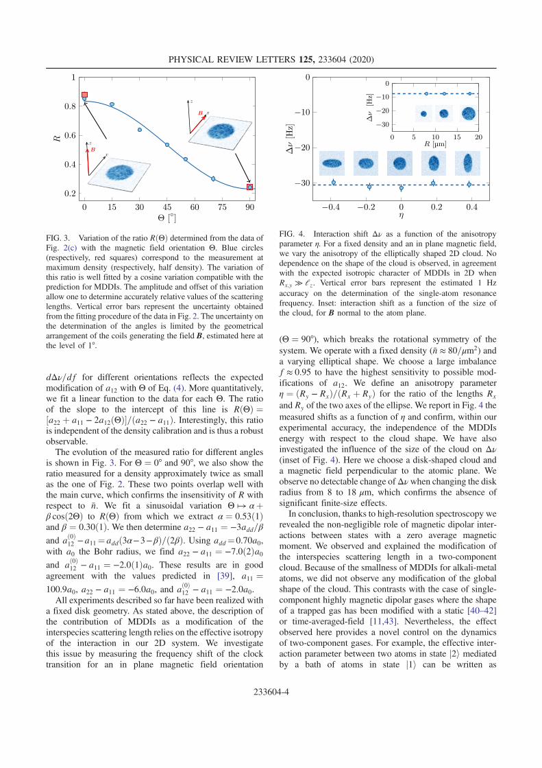
dΔν=df for different orientations reflects the expectedmodification of a12 with Θ of Eq. (4). More quantitatively,we fit a linear function to the data for each Θ. The ratioof the slope to the intercept of this line is RðΘÞ ¼½a22 þ a11 − 2a12ðΘÞ=ða22 − a11Þ. Interestingly, this ratiois independent of the density calibration and is thus a robustobservable.The evolution of the measured ratio for different angles

is shown in Fig. 3. For Θ ¼ 0° and 90°, we also show theratio measured for a density approximately twice as smallas the one of Fig. 2. These two points overlap well withthe main curve, which confirms the insensitivity of R withrespect to n. We fit a sinusoidal variation Θ ↦ αþβ cosð2ΘÞ to RðΘÞ from which we extract α ¼ 0.53ð1Þand β ¼ 0.30ð1Þ. We then determine a22 − a11 ¼ −3add=βand að0Þ12 −a11¼addð3α−3−βÞ=ð2βÞ. Using add¼0.70a0,with a0 the Bohr radius, we find a22 − a11 ¼ −7.0ð2Þa0and að0Þ12 − a11 ¼ −2.0ð1Þa0. These results are in goodagreement with the values predicted in [39], a11 ¼100.9a0, a22 − a11 ¼ −6.0a0, and að0Þ12 − a11 ¼ −2.0a0.All experiments described so far have been realized with

a fixed disk geometry. As stated above, the description ofthe contribution of MDDIs as a modification of theinterspecies scattering length relies on the effective isotropyof the interaction in our 2D system. We investigatethis issue by measuring the frequency shift of the clocktransition for an in plane magnetic field orientation

(Θ ¼ 90°), which breaks the rotational symmetry of thesystem. We operate with a fixed density (n ≈ 80=μm2) anda varying elliptical shape. We choose a large imbalancef ≈ 0.95 to have the highest sensitivity to possible mod-ifications of a12. We define an anisotropy parameterη ¼ ðRy − RxÞ=ðRx þ RyÞ for the ratio of the lengths Rx

and Ry of the two axes of the ellipse. We report in Fig. 4 themeasured shifts as a function of η and confirm, within ourexperimental accuracy, the independence of the MDDIsenergy with respect to the cloud shape. We have alsoinvestigated the influence of the size of the cloud on Δν(inset of Fig. 4). Here we choose a disk-shaped cloud anda magnetic field perpendicular to the atomic plane. Weobserve no detectable change ofΔνwhen changing the diskradius from 8 to 18 μm, which confirms the absence ofsignificant finite-size effects.In conclusion, thanks to high-resolution spectroscopy we

revealed the non-negligible role of magnetic dipolar inter-actions between states with a zero average magneticmoment. We observed and explained the modification ofthe interspecies scattering length in a two-componentcloud. Because of the smallness of MDDIs for alkali-metalatoms, we did not observe any modification of the globalshape of the cloud. This contrasts with the case of single-component highly magnetic dipolar gases where the shapeof a trapped gas has been modified with a static [40–42]or time-averaged-field [11,43]. Nevertheless, the effectobserved here provides a novel control on the dynamicsof two-component gases. For example, the effective inter-action parameter between two atoms in state j2i mediatedby a bath of atoms in state j1i can be written as

FIG. 3. Variation of the ratio RðΘÞ determined from the data ofFig. 2(c) with the magnetic field orientation Θ. Blue circles(respectively, red squares) correspond to the measurement atmaximum density (respectively, half density). The variation ofthis ratio is well fitted by a cosine variation compatible with theprediction for MDDIs. The amplitude and offset of this variationallow one to determine accurately relative values of the scatteringlengths. Vertical error bars represent the uncertainty obtainedfrom the fitting procedure of the data in Fig. 2. The uncertainty onthe determination of the angles is limited by the geometricalarrangement of the coils generating the field B, estimated here atthe level of 1°.

FIG. 4. Interaction shift Δν as a function of the anisotropyparameter η. For a fixed density and an in plane magnetic field,we vary the anisotropy of the elliptically shaped 2D cloud. Nodependence on the shape of the cloud is observed, in agreementwith the expected isotropic character of MDDIs in 2D whenRx;y ≫ lz. Vertical error bars represent the estimated 1 Hzaccuracy on the determination of the single-atom resonancefrequency. Inset: interaction shift as a function of the size ofthe cloud, for B normal to the atom plane.


233604-4

geff22 ¼ g22 − g212=g11, where gij ¼ffiffiffiffiffiffi8π

paij=lz [44]. With

our parameters, we achieve a variation by a factor 7 ofgeff22 , which will lead to important modifications of polarondynamics. Similarly, it can be exploited to tune themiscibility of mixtures or the dynamics of spin textures.The distance to the critical point for miscibility, whoseposition is given by g22g11 ¼ g212, is also strongly sensitiveto a variation of g12. For instance, the length scale of spintextures appearing in phase separation dynamics of abalanced mixture will be modified, for our parameters,by a factor of almost 3 when Θ is switched from 0° to 90°[34]. In addition, one can exploit the nonlocal character ofMDDIs by confining the atoms in a deep lattice at unitfilling, where the exchange coupling evidenced here willimplement the so-called quantum XX model [45] withoutrequiring any tunneling between lattice sites. The extremesensitivity of the clock transition and its protection frommagnetic perturbations will then provide a novel, precisetool to detect the various phases of matter predicted withinthis model.

This work is supported by ERC (Synergy UQUAM),European Union's Horizon 2020 Programme (QuantERA-NAQUAS project), and the ANR-18-CE30-0010 grant. Wethank F. Pereira dos Santos, M. Zwierlein, and P. Juliennefor stimulating discussions. We acknowledge the contri-bution of R. Saint-Jalm at the early stage of the project.

*[email protected][1] C. Chin, R. Grimm, P. Julienne, and E. Tiesinga, Feshbach

resonances in ultracold gases, Rev. Mod. Phys. 82, 1225(2010).

[2] I. Bloch, J. Dalibard, and W. Zwerger, Many-body physicswith ultracold gases, Rev. Mod. Phys. 80, 885 (2008).

[3] K. Baumann, C. Guerlin, F. Brennecke, and T. Esslinger,Dicke quantum phase transition with a superfluid gas in anoptical cavity, Nature (London) 464, 1301 (2010).

[4] R. Löw, H. Weimer, J. Nipper, J. B. Balewski, B. Butscher,H. P. Büchler, and T. Pfau, An experimental and theoreticalguide to strongly interacting Rydberg gases, J. Phys. B 45,113001 (2012).

[5] T. Lahaye, C. Menotti, L. Santos, M. Lewenstein, andT. Pfau, The physics of dipolar bosonic quantum gases,Rep. Prog. Phys. 72, 126401 (2009).

[6] I. Ferrier-Barbut, H. Kadau, M. Schmitt, M. Wenzel, and T.Pfau, Observation of Quantum Droplets in a StronglyDipolar Bose Gas, Phys. Rev. Lett. 116, 215301 (2016).

[7] L. Chomaz, R. M.W. van Bijnen, D. Petter, G. Faraoni, S.Baier, J. H. Becher, M. J. Mark, F. Waechtler, L. Santos, andF. Ferlaino, Observation of Roton mode population in adipolar quantum gas, Nat. Phys. 14, 442 (2018).

[8] A. de Paz, A. Sharma, A. Chotia, E. Marechal, J. H.Huckans, P. Pedri, L. Santos, O. Gorceix, L. Vernac, andB. Laburthe-Tolra, Nonequilibrium Quantum Magnetism ina Dipolar Lattice Gas, Phys. Rev. Lett. 111, 185305 (2013).

[9] S. Baier, M. J. Mark, D. Petter, K. Aikawa, L. Chomaz,Z. Cai, M. Baranov, P. Zoller, and F. Ferlaino, ExtendedBose-Hubbard models with ultracold magnetic atoms,Science 352, 201 (2016).

[10] S. Lepoutre, J. Schachenmayer, L. Gabardos, B. Zhu, B.Naylor, E. Marechal, O. Gorceix, A. M. Rey, L. Vernac, andB. Laburthe-Tolra, Out-of-equilibrium quantum magnetismand thermalization in a spin-3 many-body dipolar latticesystem, Nat. Commun. 10, 1714 (2019).

[11] S. Giovanazzi, A. Görlitz, and T. Pfau, Tuning the DipolarInteraction in Quantum Gases, Phys. Rev. Lett. 89, 130401(2002).

[12] M. Fattori, G.Roati, B.Deissler, C.D’Errico,M.Zaccanti,M.Jona-Lasinio, L. Santos, M. Inguscio, and G. Modugno,Magnetic Dipolar Interaction in a Bose-Einstein CondensateAtomic Interferometer, Phys. Rev. Lett. 101, 190405 (2008).

[13] S. E. Pollack, D. Dries, M. Junker, Y. P. Chen, T. A.Corcovilos, and R. G. Hulet, Extreme Tunability of Inter-actions in a 7Li Bose-Einstein Condensate, Phys. Rev. Lett.102, 090402 (2009).

[14] D. M. Stamper-Kurn and M. Ueda, Spinor Bose gases:Symmetries, magnetism, and quantum dynamics, Rev. Mod.Phys. 85, 1191 (2013).

[15] S. Yi, L. You, and H. Pu, Quantum Phases of Dipolar SpinorCondensates, Phys. Rev. Lett. 93, 040403 (2004).

[16] M. Vengalattore, S. R. Leslie, J. Guzman, and D. M.Stamper-Kurn, Spontaneously Modulated Spin Texturesin a Dipolar Spinor Bose-Einstein Condensate, Phys.Rev. Lett. 100, 170403 (2008).

[17] Y. Eto, H. Saito, and T. Hirano, Observation of Dipole-Induced Spin Texture in an 87Rb Bose-Einstein Condensate,Phys. Rev. Lett. 112, 185301 (2014).

[18] G. E. Marti, A. MacRae, R. Olf, S. Lourette, F. Fang, andD.M. Stamper-Kurn, Coherent Magnon Optics in a Ferro-magnetic Spinor Bose-Einstein Condensate, Phys. Rev.Lett. 113, 155302 (2014).

[19] B. Yan, S. A. Moses, B. Gadway, J. P. Covey, K. R. A.Hazzard, A. M. Rey, D. S. Jin, and J. Ye, Observation ofdipolar spin-exchange interactions with lattice-confinedpolar molecules, Nature (London) 501, 521 (2013).

[20] S. de Leseleuc, D. Barredo, V. Lienhard, A. Browaeys, andT. Lahaye, Optical Control of the Resonant Dipole-DipoleInteraction between Rydberg Atoms, Phys. Rev. Lett. 119,053202 (2017).

[21] For all experiments reported here, the fraction of atoms inany other spin state remains below our detection sensitivityof 1%.

[22] See SupplementalMaterial at http://link.aps.org/supplemental/10.1103/PhysRevLett.125.233604 for details on the calcula-tion of the effective interspecies scattering length a12.

[23] U. R. Fischer, Stability of quasi-two-dimensional Bose-Einstein condensates with dominant dipole-dipole inter-actions, Phys. Rev. A 73, 031602(R) (2006).

[24] A. K. Fedorov, I. L. Kurbakov, Y. E. Shchadilova, and Yu. E.Lozovik, Two-dimensional Bose gas of tilted dipoles: Rotoninstability and condensate depletion, Phys. Rev. A 90,043616 (2014).

[25] C. Mishra and R. Nath, Dipolar condensates with tilteddipoles in a pancake-shaped confinement, Phys. Rev. A 94,033633 (2016).


233604-5

[26] S. Yi and L. You, Trapped atomic condensates withanisotropic interactions, Phys. Rev. A 61, 041604(R)(2000).

[27] We use the definition of Ref. [5]. Other definitions with adifferent numerical factor are found in the literature, see forinstance, [28,29].

[28] D. C. E. Bortolotti, S. Ronen, J. L. Bohn, and D. Blume,Scattering Length Instability in Dipolar Bose-EinsteinCondensates, Phys. Rev. Lett. 97, 160402 (2006).

[29] M. A. Baranov, M. Dalmonte, G. Pupillo, and P. Zoller,Condensed matter theory of dipolar quantum gases, Chem.Rev. 112, 5012 (2012).

[30] J. L. Ville, T. Bienaime, R. Saint-Jalm, L. Corman, M.Aidelsburger, L. Chomaz, K. Kleinlein, D. Perconte, S.Nascimbene, J. Dalibard, and J. Beugnon, Loading andcompression of a single two-dimensional Bose gas in anoptical accordion, Phys. Rev. A 95, 013632 (2017).

[31] R. Saint-Jalm, P. C. M. Castilho, É. Le Cerf, B. Bakkali-Hassani, J.-L. Ville, S. Nascimbene, J. Beugnon, and J.Dalibard, Dynamical Symmetry and Breathers in a Two-Dimensional Bose Gas, Phys. Rev. X 9, 021035 (2019).

[32] D. M. Harber, H. J. Lewandowski, J. M. McGuirk, and E. A.Cornell, Effect of cold collisions on spin coherence andresonance shifts in a magnetically trapped ultracold gas,Phys. Rev. A 66, 053616 (2002).

[33] The imbalance f is tuned mostly by changing the pulseduration but for small pulses area it is more convenient toalso decrease the Rabi frequency to avoid using very shortmicrowave pulses.

[34] E. Timmermans, Phase Separation of Bose-Einstein Con-densates, Phys. Rev. Lett. 81, 5718 (1998).

[35] At nonzero temperature, quantum statistics of thermalbosons lead to multiply this shift by a factor which variesfrom 1 in the very degenerate regime to 2 for a thermalcloud.

[36] M. J. Martin, M. Bishof, M. D. Swallows, X. Zhang, C.Benko, J. von Stecher, A. V. Gorshkov, A. M. Rey, andJ. Ye, A quantum many-body spin system in an opticallattice clock, Science 341, 632 (2013).

[37] R. J. Fletcher, R. Lopes, J. Man, N. Navon, R. P. Smith,M.W. Zwierlein, and Z. Hadzibabic, Two- and three-bodycontacts in the unitary Bose gas, Science 355, 377 (2017).

[38] Y.-Q. Zou, B. Bakkali-Hassani, C. Maury, É. Le Cerf, S.Nascimbene, J. Dalibard, and J. Beugnon, Tan’s two-bodycontact across the superfluid transition of a planar Bose gas,arXiv:2007.12385.

[39] P. A. Altin, G. McDonald, D. Döring, J. E. Debs, T. H.Barter, J. D. Close, N. P. Robins, S. A. Haine, T. M. Hanna,and R. P. Anderson, Optically trapped atom interferometryusing the clock transition of large 87Rb Bose-Einsteincondensates, New J. Phys. 13, 065020 (2011).

[40] D. H. J. O’Dell, S. Giovanazzi, and C. Eberlein, ExactHydrodynamics of a Trapped Dipolar Bose-EinsteinCondensate, Phys. Rev. Lett. 92, 250401 (2004).

[41] J. Stuhler, A. Griesmaier, T. Koch, M. Fattori, T. Pfau, S.Giovanazzi, P. Pedri, and L. Santos, Observation of Dipole-Dipole Interaction in a Degenerate Quantum Gas, Phys.Rev. Lett. 95, 150406 (2005).

[42] T. Lahaye, T. Koch, B. Fröhlich, M. Fattori, J. Metz, A.Griesmaier, S. Giovanazzi, and T. Pfau, Strong dipolareffects in a quantum ferrofluid, Nature (London) 448, 672(2007).

[43] Y. Tang, W. Kao, K. Y. Li, and B. L. Lev, Tuning the Dipole-Dipole Interaction in a Quantum Gas with a RotatingMagnetic Field, Phys. Rev. Lett. 120, 230401 (2018).

[44] C. J. Pethick and H. Smith, Bose-Einstein Condensation inDilute Gases (Cambridge University Press, Cambridge,England, 2008).

[45] S. Sachdev, Quantum Phase Transitions (CambridgeUniversity Press, Cambridge, England, 2006).


233604-6

Journal of Physics B: Atomic, Molecular and Optical Physics

J. Phys. B: At. Mol. Opt. Phys. 54 (2021) 08LT01 (7pp) https://doi.org/10.1088/1361-6455/abf298

Letter

Optical control of the density and spinspatial profiles of a planar Bose gas

Y-Q Zou1,4, É Le Cerf1,4, B Bakkali-Hassani1, C Maury1, G Chauveau1,P C M Castilho2, R Saint-Jalm3, S Nascimbene1 , J Dalibard1 andJ Beugnon1,∗

1 Laboratoire Kastler Brossel, College de France, CNRS, ENS-PSL University, Sorbonne Universite, 11Place Marcelin Berthelot, 75005 Paris, France2 Instituto de Física de Sao Carlos, Universidade de Sao Paulo, CP 369, 13560-970 Sao Carlos, Brazil3 Department of Physics, Ludwig-Maximilians-Universitat München, Schellingstr. 4, D-80799 München,Germany

E-mail: [email protected]

Received 13 February 2021, revised 19 March 2021Accepted for publication 25 March 2021Published 30 April 2021

AbstractWe demonstrate the arbitrary control of the density profile of a two-dimensional Bose gas byshaping the optical potential applied to the atoms. We use a digital micromirror device (DMD)directly imaged onto the atomic cloud through a high resolution imaging system. Ourapproach relies on averaging the response of many pixels of the DMD over the diffraction spotof the imaging system, which allows us to create an optical potential with an arbitrary intensityprofile and with micron-scale resolution. The obtained density distribution is optimized with afeedback loop based on the measured absorption images of the cloud. Using the same device,we also engineer arbitrary spin distributions thanks to a two-photon Raman transfer betweeninternal ground states.

Keywords: quantum gases, spatial light modulator, spin textures

(Some figures may appear in colour only in the online journal)

1. Introduction

Ultracold quantum gases are ideal platforms to study physi-cal phenomena, thanks to their high flexibility and their isola-tion from the environment. They are widely used for quantumsimulations [1] and metrological applications [2]. Various trapgeometries have been realized to confine atomic clouds. His-torically, harmonic confinements have been the norm in coldatom experiments due to their ease of implementation [3, 4].

4 These authors contributed equally to this work.∗ Author to whom any correspondence should be addressed.

The recent realization of uniform systems opened new per-spectives to explore the thermodynamic properties and dynam-ical behavior of quantum gases [5–8]. Other trap potentialshave been applied to explore physics in specific geometries,such as supercurrents in ring potentials [9–12], analog sonicblack holes in more complex potentials [13], and low-entropyphases in lattice systems [14].

In the past years, several approaches have been developedto generate complex optical potential profiles [15–22]. Mostof them rely on the development of spatial light modula-tors, which can modulate the phase or the intensity of a lightbeam. Digital micromirror devices (DMDs) are one of the mostwidely used in cold atom experiments thanks to their low cost,simple use and high refresh rates. They consist of millions ofindividual micromirrors which can be set in two different ori-

0953-4075/21/08LT01+7$33.00 1 © 2021 IOP Publishing Ltd Printed in the UK

J. Phys. B: At. Mol. Opt. Phys. 54 (2021) 08LT01

Figure 1. Sketch of the experimental setup for arbitrary densitycontrol. Two DMDs are used to project an optical potential onto theatoms with a high NA microscope objective (objective 1). Both ofthem are illuminated by a blue-detuned 532 nm laser. DMD1provides the hard-wall potential, while DMD2 adds an additionalpotential for density control. The light fields from the two DMDs aremixed on a polarizing beam splitter with orthogonal polarizations sothat they do not interfere with each other. The atoms are imagedonto the camera with a second identical objective (objective 2). Weuse absorption imaging to measure the 2D density profiles on a CCDcamera.

entations, hence corresponding to a ‘black’ or ‘white’ signal ina chosen image plane of the DMD chip. They have been used tocorrect optical aberrations when working as a programmableamplitude hologram in a Fourier plane [23], and to producedifferent potential profiles by direct imaging [21, 24–26].

In this article, we demonstrate arbitrary control of the den-sity profile of two-dimensional (2D) Bose gases by tailoringthe in-plane trapping potential using DMDs. We program apattern on the DMD chip and simply image it onto the atomiccloud. The limitation due to the binary status of the DMD pix-els (black or white) is overcome by realizing a spatial averageof the response of ∼25 pixels over the point spread function ofthe imaging system. This gives us access to several levels ofgrey for the optical potential at a given position in the atomicplane. The DMD pattern is computed thanks to an error diffu-sion algorithm combined with a feedback loop to directly opti-mize the measured atomic density distribution. The method isproved to be efficient and robust to optical imperfections. Inaddition, we demonstrate the realization of arbitrary spin dis-tributions with the same protocol by using spatially resolvedtwo-photon Raman transitions.

2. Apparatus and main results

We work with a degenerate 2D Bose gas of 87Rb atoms. Themain experimental setup has been described previously in[27, 28]. Briefly, about 105 Rb atoms in the F = 1, m = 0hyperfine ground state are loaded into a 2D box potential.The vertical confinement is provided by a vertical lattice. Allatoms are trapped around a single node of the lattice in anapproximately harmonic potential with a measured trap fre-

quency ωz/2π = 4.1(1) kHz. The in-plane trap is providedby a hard-wall potential created by a first DMD (DMD1 inthe following)5. All laser beams used for creating the 2Dbox potential have a wavelength of 532 nm and thus repelRb atoms from high intensity regions. The cloud temperatureis controlled by lowering the in-plane potential height, thusenabling evaporative cooling. We reach temperatures below30 nK and an average 2D atom density of ∼80 μm−2, corre-sponding to a regime where the cloud is well described by theThomas–Fermi approximation. Both the interaction energyand thermal energy are smaller than the vertical trapping fre-quency and the atom cloud is thus in the so-called quasi-2Dregime.

We show in figure 1 a sketch of the experimental setupfor arbitrary density control. We modify the density distribu-tion by using another DMD (DMD2) to impose an additionalrepulsive optical potential to the hard-wall potential made byDMD1. The pattern on DMD2 is imaged onto the atomicplane thanks to an imaging system of magnification ≈1/70.The pixel size of DMD2 is 13.7 μm, leading to an effectivesize of 0.2 μm in the atomic plane. The numerical aperture(NA ∼ 0.4) is limited by a microscope objective above thevacuum glass cell containing the atoms and leads to a spatialresolution around 1 μm. Consequently, the area defined by thediffraction spot of the imaging system typically corresponds toa region where 5 × 5 pixels of DMD2 are imaged, which makespossible the realization of grey levels of light intensity. DMD2is illuminated by a blue-detuned 532 nm laser with a waist ofw ∼ 55 μm in the atomic plane. The intensity of the beam isset to provide a maximum repulsive potential around 2μ whereμ is the chemical potential of the gas for a density of 80 μm−2.The potential is added before the final evaporation stage in thebox potential.

The 2D atomic density profile is obtained by absorptionimaging with a second identical microscope objective placedbelow the glass cell. This imaging system has a similar opti-cal resolution and the effective pixel size of the camera inthe atomic plane is 1.15 μm. We probe the atoms in the trapusing a 10 μs pulse of light on the D2 line resonant betweenthe F = 2 ground state and the F′ = 3 excited state. Beforedetection, a microwave pulse is applied to transfer a controlledfraction of atoms into the ground level from F = 1, m = 0to F = 2, m = 0, which thus absorbs light from the imagingbeam. The transferred fraction is controlled so that the mea-sured optical depth (OD) is always smaller than 1.5 to reducenonlinear imaging effects.

Figure 2 presents a selection of 2D density profilesrealized in our experiment. For each example, we showin figures 2(a)–(d) averaged absorption images and infigures 2(e)–(h) the corresponding mean OD integrated alongone or two spatial directions. Figure 2(a) shows a uniform pro-file in which we have corrected the inhomogeneities caused byresidual defects of the overall box potential created by the com-bination of DMD1 and vertical lattice beams. Figures 2(b)–(d)

5 All DMDs used in this work are DLP7000 from Texas Instruments andinterfaced by Vialux GmbH.

2


Figure 2. Various density profiles realized in our experiment. From left to right, we show a uniform profile and linearly varying densityprofiles along x, along the radial direction and along the azimuthal direction. (a)–(d) Averaged absorption images (50, 99, 50, 20 shotsrespectively). (e)–(h) Corresponding OD profiles integrated over one direction (x and y in (e) and (f), azimuthal in (g) and radial in (h)). Thesolid lines represent the OD profiles of the target density distributions. Error bars show the statistical error corresponding to one standarderror of the mean.

Figure 3. (a) Diagram of the iterative algorithm. (b) Example ofgrey-level profile Gn obtained during the optimization loop used tocreate the linearly varying profile shown in figure 2(b).(c) Corresponding dithered image computed with the error diffusionalgorithm and programmed on the DMD. The grey level ranges from0 to 1, with an effective pixel size of 1.15 μm equal to the one of theabsorption image. The DMD pattern is binary with an effective pixelsize of 0.2 μm.

correspond to linearly varying density distributions respec-tively along the x direction, along the radial direction and alongthe azimuthal direction.

3. Detailed implementation

One could naively think that for a given target density pro-file, the suitable pattern on DMD2 could be directly computedand imaged onto the atoms. However, several features preventsuch a simple protocol. First, the DMD is a binary modulator.Then, for a finite number of pixels, it is not possible to createan arbitrary grey-level pattern with perfect accuracy. Here, weuse the well-known error diffusion technique to generate thebinary pattern for a given grey-level profile [29, 30] (see theappendix for a short description). Second, the imaging systemfrom DMD2 to the atoms has an optical response that leads toa modification of the ideal image, mainly because of the finiteaperture of the optical elements. Third, any imperfection on theoptical setup (inhomogeneity of the laser beam, optical aber-rations. . . ) also degrades the imaging of the DMD pattern ontothe atomic cloud. Finally, the atomic density distribution isobtained through absorption imaging, which adds noise mostlycoming from the photonic shot noise induced by the imagingbeam. Hence, an iterative method is needed to obtain the opti-mal DMD pattern that gives a density distribution as close aspossible to the target. The working principle of the optimiza-tion loop is simply to add (remove) light at the positions wherethere are more (fewer) atoms than the target until the densityprofile converges to the target one.

Figure 3(a) shows the steps of the iterative loop. Thebasic idea of each step n consists in computing the differencebetween the measured density distribution An and the targetimage Tn, and adding it with a suitable gain K to the previousgrey-level intensity profile Gn. This gives the grey-level profileof iteration n + 1 (see figure 3(b)),

Gn+1 = Gn + K(An − Tn), (1)

3


Figure 4. Convergence of the iterative algorithm. (a) Plot of Fm, Nd

and F with iteration number. Target profile is a linear densitydistribution along x in a square box (of figure 2(b)). F convergesvery fast and stays around 0.06 after iteration 6. Nd decreasessuddenly at iteration 8 and 15 because Na (number of absorptionimages for averaging) changes from 5 to 10 at iteration 8 and to 99at iteration 15. For Fm, we show the estimated statistical error barsto give an illustrative indication of our typical uncertainties. Theseerror bars are obtained from a bootstrap approach on the differentrepetitions of the experiment in the same conditions. (b) For the lastiteration (iteration 15), we plot Fm, Nd and F versus the number ofimages Na used for averaging. Both Fm and Nd decrease with Nawhile F does not depend on Na. (c) Evolution of F for different K′

0s.

which is then discretized thanks to the error diffusionalgorithm (see figure 3(c)) and imaged onto the atoms. Besidesthis general idea, we detail below some specific features of ourloop:

• We initialize the optimization with a grey-level profile G0

which can either be uniformly 0 or 1.• To avoid border effects, we select on the absorption

images a region slightly inside the box potential (two pix-els smaller in each direction) for density control and weextrapolate the grey-level profile Gn outside the box. Theextrapolation is done by simply duplicating the value ofthe outermost pixels of Gn by three more pixels along eachside for a square box or along the radial direction for adisk.

• The image An of the density distribution is obtained fromthe average of several repetitions of the experiment with

the same parameters to limit the contribution of detectionnoise.

• The measured image of the atomic distribution is convo-luted with a Gaussian function of rms width 1 pixel of thecamera of the imaging system. This convolution acts as alow pass filter which reduces high spatial frequency noise,especially detection noise.

• Considering the Gaussian shape of the beam illuminatedon DMD, we choose K to be position dependent K(x, y) =

K0 × e2[(x−x0)2+(y−y0)2]

w2 , where w is the waist of the beamin the atomic plane and x0 and y0 are the coordinatesof the center of the beam. It makes the effective gainapproximately the same for all the pixels.

• At each iteration, we rescale the amplitude of the targetprofile to obtain the same mean OD as the one of An. Thisavoids taking into account errors coming from the shot-to-shot variation of the atom number which would leadto a global error that we are not interested in. Note thatthis variation is smaller than 10% during the optimizationloop.

4. Characterization of the loop

We stop the optimization loop when the measured densitydistribution has converged to the target one, up to a prede-fined precision. To estimate the deviation from the target, wedefine a figure of merit Fm corresponding to the measuredroot-mean-square deviation:

Fm =

√Npix

∑(i, j)∈A(OD(i, j) − ODT (i, j))2

(∑

(i, j)∈AOD(i, j))2, (2)

where A is the region of interest containing Npix pixels andOD(i, j) (resp. ODT(i, j)) is the measured average OD (resp.target OD). The value of the figure of merit Fm results fromtwo kinds of contributions. Obviously, there is the actual devi-ation of the density distribution from the target. In addition,several features of the measurement method give an unde-sired contribution to Fm. Indeed, thermal fluctuations of theatomic cloud, projection noise due the partial transfer imag-ing discussed above and photonic shot noise in absorptionimaging lead to unavoidable residual noise. For our parame-ters, we computed in a separate work that the two dominantmechanisms are photonic and projection noise with a similarweight, whose exact values depend on the studied density dis-tribution. In the low temperature regime explored here thermalfluctuations are almost negligible.

The contributions coming from photonic shot noise andprojection noise can be reduced by averaging more images.However, for the typical repetition rate of our experiment (∼30 s), the number of averaged images has to be limited to a fewtens for realistic applications. To characterize the optimizationloop, we compute this noise contribution Nd so as to remove itfrom the measured Fm. We directly estimate Nd from the set ofimages taken with the same parameters by computing the dis-persion of the measured absorption images from the averagedimage,

4


Nd =

√Npix

∑k

∑(i, j)∈A(ODk(i, j) − OD(i, j))2

N2a (

∑(i, j)∈AOD(i, j))2

, (3)

where the index k refers to the kth absorption image amongthe Na pictures taken for the average. We thus define thecorrected figure of merit:

F =√

F2m − N 2

d , (4)

which quantifies the distance of the density profile from thetarget while removing measurement noise.

In figure 4(a), we show the evolution of Fm, Nd and F asa function of the number of iterations in the example case of alinear profile in a square box (as shown in figure 2(b)). We ini-tialize the loop with a grey-level profile equal to zero and wechoose K0 = 0.2. The number of pictures which are averagedis 5 for the first 7 iterations, 10 up to iteration 14 and 99 forthe last iteration. This leads to clear jumps of Nd with the iter-ation number. Interestingly, we see that F converges almostmonotonously to about 0.06 after the first 6 iterations and thenstays approximately constant whatever the value of Na is. Thisindicates that the contribution of measurement noise is wellsubtracted. This is confirmed in figure 4(b), where we plot Fm,Nd and F as a function of Na using the data of the final itera-tion of figure 4(a). As expected, both Fm and Nd decrease withNa while F does not change.

We also studied the behavior of the iterative loop with dif-ferent K′

0s varying from 0.1 to 0.6. The convergence of F isplotted in figure 4(c). The iterative algorithm works well fora large range of values of K0. We observe that increasing K0

speeds up the convergence, but too large values of K0 leadto strong local variations in the measured images. In prac-tice, for most target distributions, we use K0 = 0.2 as a goodcompromise between these two trends.

In the appendix, we study through simple numerical simu-lations the remaining limitations that contribute to the exper-imentally obtained F . The main limitation comes from thenumber of iterations used in the experiment (∼15). We showthat the figure of merit F decreases slowly down to ∼0.02for larger iteration numbers but reaching such a limit wouldrequire prohibitively long experimental times.

5. Arbitrary spin distribution

Using a similar protocol, we also demonstrate arbitrary spindistributions by shaping a pair of copropagating Raman beamswhich couple the |F = 1, m = 0〉 (|1〉) and |F = 2, m = 0〉(|2〉) states by a two-photon Raman transition. The two Ramanbeams originate from the same laser and have a wavelengthof ∼790 nm, in between the D1 and D2 line of 87Rb atoms.One beam is frequency shifted with respect to the other by∼6.8 GHz to fulfill the two-photon resonance between thetwo states. The two beams are coupled into the same single-mode optical fiber with orthogonal linear polarizations. Afterreflection on a third DMD (DMD3, not shown in figure 1)they are overlapped with the two beams coming from DMD1and DMD2 and are imaged onto the atomic plane with amagnification of ≈1/40 and a waist of 40 μm.

Figure 5. Imprinting a spatial spin texture. We show the densitydistribution of atoms in |2〉 immersed in a bath of atoms in |1〉.The total density of the gas is uniform in a 20 μm radius disk(∼ 80 μm−2, corresponding to OD ∼ 8). The main figures show theradial profiles of component |2〉 in semilog scale for (a) a Gaussianprofile and (b) a solitary Townes profile. The solid lines are thetarget radial profiles. Error bars show the statistical errorcorresponding to one standard error of the mean. Insets show thecorresponding averaged absorption images (20 shots). The dashedlines represent the edges of the bath of atoms in |1〉.

Starting from a cloud of atoms in state |1〉 of uniform den-sity, we pulse the Raman beams with a duration of a few tensof μs to coherently transfer a controlled fraction of atoms tostate |2〉. In this protocol, the total density of the cloud remainsuniform. We then image the density distribution of atoms instate |2〉 prior to any spin dynamics and apply an optimizationprotocol identical to the one developed for creating arbitrarydensity distributions. We show in figure 5 two examples ofspin profiles realized in our system at the end of the optimiza-tion loop: a Gaussian profile (figure 5(a)) and the so-calledTownes profile (figure 5(b)), which is a solitonic solution of the2D attractive non-linear Schrödinger equation that decreasesalmost exponentially with r at large r [31]. The measured pro-files are very close to the target over typically two orders ofmagnitude in density.

6. Discussion and outlook

In conclusion, we have demonstrated the arbitrary control ofthe density profile of an ultracold 2D quantum gas by tai-loring a repulsive optical potential. We have also demon-strated the arbitrary creation of spin textures using spatiallyresolved Raman transitions. An iterative method was applied,making the method robust to technical imperfections. Theapproach described here can be straightforwardly applied toother atomic species. It opens new possibilities for studying thedynamics of single or multi-component low-dimensional gaseswhere, for instance, the presence of scale-invariance or inte-grability leads to a rich variety of non-trivial time evolutions[32–35].

Acknowledgments

This work is supported by ERC (Synergy UQUAM andTORYD), European Union’s Horizon 2020 Program (Quan-tERA NAQUAS project) and the ANR-18-CE30-0010 grant.

5


Appendix A

A.1. Error diffusion algorithm

We briefly recall in this paragraph the main features of the errordiffusion algorithm, which we use to compute the pattern pro-grammed on the DMD. Error diffusion is used to convert agrey-level image where each pixel takes arbitrary values intoan image with only zeros and ones. Starting for instance fromthe top left pixel of the image, one chooses the status of the cor-responding DMD pixel by rounding to 0 or 1 the targeted greylevel . This binary choice results in an error which is ‘diffused’to the remaining neighboring pixels with a given weight. Inthis work, we use the method developed in reference [29]. Weprocess the pixels from left to right and from top to bottom.The error made when choosing the state of a pixel (denoted bya in equation (5)) is diffused to its first right neighbor andthe three nearest neighbors of the following line with weightsgiven by

⎛⎜⎝

− 716

. . .

. . .316

516

116

. . .

⎞⎟⎠ . (5)

A.2. Simulations

In this section, we simulate the experiment to understandthe various contributions to the obtained value of the figureof merit F for the density correction. In the simulation,we start with a ‘test’ density profile A0, which is obtainedfrom an experiment with DMD2 being off. It is an averagedimage of 100 experimental shots so that the detection noiseis mostly averaged out. We follow the same procedure whichwas described in figure 3(a) but in a ‘numerical experiment’.We simulate the action of the potential shaped by the DMD byusing the local density approximation in the Thomas–Fermiregime. Thus, for each iteration n of the loop we compute thedensity profile as

An = A0 − αCn, (6)

where Cn is the light intensity profile given by the DMD pat-tern after a convolution step that simulates the finite numericalaperture of the optical system. We use here a Gaussian profilewith an rms width σ = 0.5 μm. The parameter α is introducedto represent the effect of the light potential on the atomic den-sity. We use as an input to the simulation experimental imagesof the OD distribution (OD ∼ 1) and we choose α = 2 to beas close as possible to the calibrated experimental parameters.We add an offset to An to keep the mean OD constant. We alsohave the possibility to add some noise to An to simulate theexperimental fluctuations.

We show in figure 6 the simulated evolution of F as a func-tion of the iteration number. The target is a linear profile alongthe x direction, same as the one studied in figures 2(b) and 4.The blue and red curves show the simulated results with theparameters used in the experiment: K0 = 0.2 and the absorp-tion image is convolved with a Gaussian function of an rmswidth 1 pixel. For the blue curve, we add independently oneach pixel of An a Gaussian noise corresponding to Nd = 0.09,

Figure 6. Numerical simulation of the experiment. Evolution of Fas a function of iteration number with (blue) or without (red) noise.The target distribution is a linear density profile along x. Thediamond corresponds to the number of iterations used in figure 4(a).The inset shows the same curves at large iteration number.

which is the typical noise obtained in the experiment for theaverage of 10 repetitions of the sequence. For the red curve,no detection noise is added, i.e. Nd = 0. The marker on the redcurve corresponds to the point when the iterative loop is ter-minated for the experimental data shown in figure 4(a). Here,F = 0.046, in qualitative good agreement with the obtainedexperimental value of 0.06.

We finally discuss the limitations to the obtained figure ofmerit. We show in the inset of figure 6 the evolution of thefigure of merit at large iteration number. Better values (∼0.02)are obtained for larger number of iterations (∼600) but with aslow convergence largely hidden by the typical experimentalnoise. This regime is not reachable in practice with our typicalexperimental cycle time. The residual value could be explainedby the filtering made when convolving the absorption imageand also by the residual defects coming from the error diffusionprotocol.

ORCID iDs

S Nascimbene https://orcid.org/0000-0002-3931-9436J Beugnon https://orcid.org/0000-0003-1701-8533

References

[1] Bloch I, Dalibard J and Nascimbene S 2012 Quantumsimulations with ultracold quantum gases Nat. Phys. 8267–76

[2] Cronin A D, Schmiedmayer J and Pritchard D E 2009 Optics andinterferometry with atoms and molecules Rev. Mod. Phys. 811051–129

[3] Pritchard D E 1983 Cooling neutral atoms in a magnetic trap forprecision spectroscopy Phys. Rev. Lett. 51 1336–9

[4] Grimm R, Weidemüller M and Ovchinnikov Y B 2000 Opticaldipole traps for neutral atoms Adv. At. Mol. Opt. Phys. 4295–170

[5] Gaunt A L, Schmidutz T F, Gotlibovych I, Smith R P andHadzibabic Z 2013 Bose–Einstein condensation of atoms ina uniform potential Phys. Rev. Lett. 110 200406

[6] Chomaz L, Corman L, Bienaime T, Desbuquois R, WeitenbergC, Nascimbene S, Beugnon J and Dalibard J 2015 Emergenceof coherence via transverse condensation in a uniform quasi-two-dimensional Bose gas Nat. Commun. 6 6162

6


[7] Mukherjee B, Yan Z, Patel P B, Hadzibabic Z, Yefsah T, Struck Jand Zwierlein M W 2017 Homogeneous atomic Fermi gasesPhys. Rev. Lett. 118 123401

[8] Hueck K, Luick N, Sobirey L, Siegl J, Lompe T and Moritz H2018 Two-dimensional homogeneous Fermi gases Phys. Rev.Lett. 120 060402

[9] Ryu C, Andersen M F, Clade P, Natarajan V, Helmerson Kand Phillips W D 2007 Observation of persistent flow of aBose–Einstein condensate in a toroidal trap Phys. Rev. Lett.99 260401

[10] Moulder S, Beattie S, Smith R P, Tammuz N andHadzibabic Z 2012 Quantized supercurrent decay inan annular Bose–Einstein condensate Phys. Rev. A 86013629

[11] Corman L, Chomaz L, Bienaime T, Desbuquois R, WeitenbergC, Nascimbene S, Dalibard J and Beugnon J 2014 Quench-induced supercurrents in an annular Bose gas Phys. Rev. Lett.113 135302

[12] Guo Y, Dubessy R, de Goër de Herve M, Kumar A, Badr T,Perrin A, Longchambon L and Perrin H 2020 Supersonicrotation of a superfluid: a long-lived dynamical ring Phys.Rev. Lett. 124 025301

[13] Lahav O, Itah A, Blumkin A, Gordon C, Rinott S, Zayats A andSteinhauer J 2010 Realization of a sonic black hole analog ina Bose–Einstein condensate Phys. Rev. Lett. 105 240401

[14] Chiu C S, Ji G, Mazurenko A, Greif D and Greiner M 2018Quantum state engineering of a Hubbard system with ultra-cold fermions Phys. Rev. Lett. 120 243201

[15] Mogensen P C and Glückstad J 2000 Dynamic array generationand pattern formation for optical tweezers Opt. Commun. 17575–81

[16] Bergamini S, Darquie B, Jones M, Jacubowiez L, BrowaeysA and Grangier P 2004 Holographic generation of micro-trap arrays for single atoms by use of a programmable phasemodulator J. Opt. Soc. Am. B 21 1889–94

[17] Pasienski M and DeMarco B 2008 A high-accuracy algorithmfor designing arbitrary holographic atom traps Opt. Express16 2176

[18] Henderson K, Ryu C, MacCormick C and Boshier M G2009 Experimental demonstration of painting arbitrary anddynamic potentials for Bose-Einstein condensates New J.Phys. 11 043030

[19] Gaunt A L and Hadzibabic Z 2012 Robust digital holographyfor ultracold atom trapping Sci. Rep. 2 721

[20] Nogrette F, Labuhn H, Ravets S, Barredo D, Beguin L, VernierA, Lahaye T and Browaeys A 2014 Single-atom trapping inholographic 2D arrays of microtraps with arbitrary geome-tries Phys. Rev. X 4 021034

[21] Gauthier G, Lenton I, McKay Parry N, Baker M, Davis M J,Rubinsztein-Dunlop H and Neely T W 2016 Direct imagingof a digital-micromirror device for configurable microscopicoptical potentials Optica 3 1136

[22] Ohl de Mello D, Schaffner D, Werkmann J, Preuschoff T,Kohfahl L, Schlosser M and Birkl G 2019 Defect-free assem-bly of 2D clusters of more than 100 single-atom quantumsystems Phys. Rev. Lett. 122 203601

[23] Zupancic P, Preiss P M, Ma R, Lukin A, Eric Tai M, RispoliM, Islam R and Greiner M 2016 Ultra-precise holographicbeam shaping for microscopic quantum control Opt. Express24 13881

[24] Jinyang L, Kohn R N, Becker M F and Heinzen D J 2009 1.5%root-mean-square flat-intensity laser beam formed usinga binary-amplitude spatial light modulator Appl. Opt. 481955–62

[25] Ha L C, Clark L W, Parker C V, Anderson B M and Chin C 2015Roton-maxon excitation spectrum of Bose condensates in ashaken optical lattice Phys. Rev. Lett. 114 055301

[26] Tajik M, Rauer B, Schweigler T, Cataldini F, Sabino J, MøllerF S, Ji S-C, Mazets I E and Schmiedmayer J 2019 Design-ing arbitrary one-dimensional potentials on an atom chip Opt.Express 27 33474

[27] Ville J L et al 2017 Loading and compression of a single two-dimensional Bose gas in an optical accordion Phys. Rev. A 95013632

[28] Ville J L, Saint-Jalm R, Le Cerf , Aidelsburger M, NascimbeneS, Dalibard J and Beugnon J 2018 Sound propagation in auniform superfluid two-dimensional Bose gas Phys. Rev. Lett.121 145301

[29] Floyd R W 1976 An adaptive algorithm for spatial grey-scaleProc. of the Society of Information Display vol 17

[30] Dorrer C and Zuegel J D 2007 Design and analysis of binarybeam shapers using error diffusion J. Opt. Soc. Am. B 241268–75

[31] Chiao R Y, Garmire E and Townes C H 1964 Self-trapping ofoptical beams Phys. Rev. Lett. 13 479

[32] Cazalilla M A, Citro R, Giamarchi T, Orignac E and RigolM 2011 One dimensional bosons: from condensed mattersystems to ultracold gases Rev. Mod. Phys. 83 1405–66

[33] Saint-Jalm R, Castilho P C M, Le Cerf É, Bakkali-Hassani B,Ville J-L, Nascimbene S, Beugnon J and Dalibard J 2019Dynamical symmetry and breathers in a two-dimensionalBose gas Phys. Rev. X 9 021035

[34] Lv C, Zhang R and Zhou Q 2020 SU(1,1) echoes for breathersin quantum gases Phys. Rev. Lett. 125 253002

[35] Shi Z-Y, Gao C and Zhai H 2020 Idealized hydrodynamics(arXiv:2011.01415)

7

188 APPENDIX H. PUBLICATIONS

Bibliography

[1] M. Arndt, O. Nairz, J. Vos-Andreae, C. Keller, G. van der Zouw &A. Zeilinger; “Wave–particle duality of C60 molecules”; Nature 401, pp. 680–682(1999). [Cited on page 11]

[2] Y. Y. Fein, P. Geyer, P. Zwick, F. Kia lka, S. Pedalino, M. Mayor, S. Ger-lich & M. Arndt; “Quantum superposition of molecules beyond 25 kDa”; NaturePhysics 15, pp. 1242–1245 (2019). [Cited on page 11]

[3] A. Shayeghi, P. Rieser, G. Richter, U. Sezer, J. H. Rodewald, P. Geyer,T. J. Martinez & M. Arndt; “Matter-wave interference of a native polypeptide”;Nature Communications 11, p. 1447 (2020). [Cited on page 11]

[4] A. Einstein; “Quantentheorie des einatomigen idealen Gases”; Sitzungsberichte derPreussischen Akademie der Wissenschaften pp. 261–267 (1924). [Cited on pages 11,17, and 37]

[5] R. P. Feynman; “Chapter II - Application of Quantum Mechanics to Liquid He-lium”; ; pp. 17–53 (Elsevier) (1955). [Cited on page 11]

[6] P. G. De Gennes; Superconductivity of Metals and Alloys; Advanced book classics(Perseus, Cambridge, MA). (1999). [Cited on pages 11 and 102]

[7] K. B. Davis, M. O. Mewes, M. R. Andrews, N. J. van Druten, D. S. Durfee,D. M. Kurn & W. Ketterle; “Bose-Einstein Condensation in a Gas of SodiumAtoms”; Physical Review Letters 75, pp. 3969–3973 (1995). [Cited on page 12]

[8] M. H. Anderson, J. R. Ensher, M. R. Matthews, C. E. Wieman & E. A.Cornell; “Observation of Bose-Einstein Condensation in a Dilute Atomic Vapor”;Science 269, pp. 198–201 (1995). [Cited on page 12]

[9] M. R. Andrews, C. G. Townsend, H.-J. Miesner, D. S. Durfee, D. M. Kurn& W. Ketterle; “Observation of Interference Between Two Bose Condensates”;Science 275, pp. 637–641 (1997). [Cited on page 12]

[10] F. Charru; Instabilites hydrodynamiques (EDP Sciences) (2021). [Cited onpage 12]

[11] J. S. Russell; “Report on Waves”; British Association for the Advancement ofScience (1845). [Cited on pages 12 and 54]

[12] N. J. Zabusky & M. D. Kruskal; “Interaction of ”Solitons” in a CollisionlessPlasma and the Recurrence of Initial States”; Physical Review Letters 15, pp. 240–243 (1965). [Cited on pages 12, 54, 56, and 109]

189

http://dx.doi.org/10.1038/44348

http://dx.doi.org/10.1038/44348

http://dx.doi.org/10.1038/s41567-019-0663-9

http://dx.doi.org/10.1038/s41567-019-0663-9

http://dx.doi.org/10.1038/s41467-020-15280-2

http://dx.doi.org/https://doi.org/10.1016/S0079-6417(08)60077-3

http://dx.doi.org/10.1103/PhysRevLett.75.3969

http://dx.doi.org/10.1126/science.269.5221.198


http://dx.doi.org/doi:10.1051/978-2-7598-0110-7



190 BIBLIOGRAPHY

[13] M. Peyrard & T. Dauxois; Physique des Solitons. (2004). [Cited on pages 12,53, and 55]

[14] Y. V. Kartashov, G. E. Astrakharchik, B. A. Malomed & L. Torner; “Fron-tiers in multidimensional self-trapping of nonlinear fields and matter”; Nature Re-views Physics 1, pp. 185–197 (2019). [Cited on pages 12 and 61]

[15] J. H. V. Nguyen, P. Dyke, D. Luo, B. A. Malomed & R. G. Hulet; “Collisionsof matter-wave solitons”; Nature Physics 10, p. 918–922 (2014). [Cited on pages 12,58, and 109]

[16] G. A. Askaryan; “Effect of the Gradient of a Strong Electromagnetic Ray onElectrons and Atoms”; Zhur. Eksptl’. i Teoret. Fiz. 42 (1962). [Cited on pages 13,57, and 60]

[17] R. Y. Chiao, E. Garmire & C. H. Townes; “Self-Trapping of Optical Beams”;Physical Review Letters 13, pp. 479–482 (1964). [Cited on pages 13, 60, and 64]

[18] V. I. Talanov; “Self-Focusing of Electromagnetic Waves in Non-Linear Media ”;Izv. Vysshikh Uchebn. Zavedenii, Radiofiz. 7 (1964). [Cited on pages 13 and 60]

[19] J. E. Bjorkholm & A. A. Ashkin; “cw Self-Focusing and Self-Trapping of Lightin Sodium Vapor”; Physical Review Letters 32, pp. 129–132 (1974). [Cited onpages 13 and 60]

[20] L. F. Mollenauer, R. H. Stolen & J. P. Gordon; “Experimental Observationof Picosecond Pulse Narrowing and Solitons in Optical Fibers”; Physical ReviewLetters 45, pp. 1095–1098 (1980). [Cited on pages 13 and 57]

[21] A. Barthelemy, S. Maneuf & C. Froehly; “Propagation soliton et auto-confinement de faisceaux laser par non linearite optique de kerr”; Optics Communi-cations 55, pp. 201–206 (1985). [Cited on pages 13 and 57]

[22] S. Burger, K. Bongs, S. Dettmer, W. Ertmer, K. Sengstock, A. Sanpera,G. V. Shlyapnikov & M. Lewenstein; “Dark Solitons in Bose-Einstein Conden-sates”; Physical Review Letters 83, pp. 5198–5201 (1999). [Cited on pages 13and 58]

[23] L. Khaykovich, F. Schreck, G. Ferrari, T. Bourdel, J. Cubizolles, L. D.Carr, Y. Castin & C. Salomon; “Formation of a Matter-Wave Bright Soliton”;Science 296, pp. 1290–1293 (2002). [Cited on pages 13 and 58]

[24] K. E. Strecker, G. B. Partridge, A. G. Truscott & R. G. Hulet; “Formationand propagation of matter-wave soliton trains”; Nature 417, p. 150–153 (2002).[Cited on pages 13, 58, and 73]

[25] N. Navon, R. P. Smith & Z. Hadzibabic; “Quantum Gases in Optical Boxes”;(2021); 2106.09716. [Cited on page 13]

[26] D. M. Stamper-Kurn & M. Ueda; “Spinor Bose gases: Symmetries, magnetism,and quantum dynamics”; Review of Modern Physics 85, pp. 1191–1244 (2013).[Cited on pages 13 and 29]

http://dx.doi.org/10.1038/s42254-019-0025-7

http://dx.doi.org/10.1038/s42254-019-0025-7

http://dx.doi.org/10.1038/nphys3135





http://dx.doi.org/https://doi.org/10.1016/0030-4018(85)90047-1



http://dx.doi.org/10.1126/science.1071021

http://dx.doi.org/10.1038/nature747

https://arxiv.org/abs/2106.09716

http://dx.doi.org/10.1103/RevModPhys.85.1191

BIBLIOGRAPHY 191

[27] A. Farolfi, D. Trypogeorgos, C. Mordini, G. Lamporesi & G. Ferrari;“Observation of Magnetic Solitons in Two-Component Bose-Einstein Condensates”;Physical Review Letters 125, p. 030401 (2020). [Cited on pages 13 and 58]

[28] X. Chai, D. Lao, K. Fujimoto, R. Hamazaki, M. Ueda & C. Raman; “MagneticSolitons in a Spin-1 Bose-Einstein Condensate”; Physical Review Letters 125, p.030402 (2020). [Cited on pages 13 and 58]

[29] C. Chin, R. Grimm, P. Julienne & E. Tiesinga; “Feshbach resonances in ultracoldgases”; Review of Modern Physics 82, pp. 1225–1286 (2010). [Cited on pages 13and 33]

[30] D. S. Petrov; “Quantum Mechanical Stabilization of a Collapsing Bose-Bose Mix-ture”; Physical Review Letters 115, p. 155302 (2015). [Cited on pages 13, 60, 61,106, and 115]

[31] C. R. Cabrera, L. Tanzi, J. Sanz, B. Naylor, P. Thomas, P. Cheiney & L. Tar-ruell; “Quantum liquid droplets in a mixture of Bose-Einstein condensates”; Sci-ence 359, pp. 301–304 (2018). [Cited on pages 13 and 61]

[32] G. Semeghini, G. Ferioli, L. Masi, C. Mazzinghi, L. Wolswijk, F. Minardi,M. Modugno, G. Modugno, M. Inguscio & M. Fattori; “Self-Bound QuantumDroplets of Atomic Mixtures in Free Space”; Physical Review Letters 120, p. 235301(2018). [Cited on pages 13 and 61]

[33] I. Ferrier-Barbut, H. Kadau, M. Schmitt, M. Wenzel & T. Pfau; “Observa-tion of Quantum Droplets in a Strongly Dipolar Bose Gas”; Physical Review Letters116, p. 215301 (2016). [Cited on pages 14 and 61]

[34] L. Chomaz, S. Baier, D. Petter, M. J. Mark, F. Wachtler, L. Santos &F. Ferlaino; “Quantum-Fluctuation-Driven Crossover from a Dilute Bose-EinsteinCondensate to a Macrodroplet in a Dipolar Quantum Fluid”; Physical Review X 6,p. 041039 (2016). [Cited on pages 14 and 61]

[35] M. Casas & S. Stringari; “Elementary excitations of 4He clusters”; Journal ofLow Temperature Physics 79, pp. 135–149 (1990). [Cited on pages 14 and 109]

[36] G. E. Volovik; The Universe in a Helium Droplet ; International Series of Mono-graphs on Physics (Oxford University Press, Oxford) (2009). [Cited on pages 14and 109]

[37] M. Barranco, R. Guardiola, S. Hernandez, R. Mayol, J. Navarro & M. Pi;“Helium Nanodroplets: An Overview”; Journal of Low Temperature Physics 142,p. 1 (2006). [Cited on pages 14 and 109]

[38] A. J. Leggett; “Can a Solid Be ”Superfluid”?” Physical Review Letters 25, pp.1543–1546 (1970). [Cited on page 14]

[39] Y. Pomeau & S. Rica; “Dynamics of a model of supersolid”; Physical ReviewLetters 72, pp. 2426–2429 (1994). [Cited on page 14]

[40] L. Chomaz, D. Petter, P. Ilzhofer, G. Natale, A. Trautmann, C. Politi,G. Durastante, R. M. W. van Bijnen, A. Patscheider, M. Sohmen, M. J.Mark & F. Ferlaino; “Long-Lived and Transient Supersolid Behaviors in DipolarQuantum Gases”; Physical Review X 9, p. 021012 (2019). [Cited on page 14]






http://dx.doi.org/10.1126/science.aao5686

http://dx.doi.org/10.1126/science.aao5686





http://dx.doi.org/10.1103/PhysRevX.6.041039


http://dx.doi.org/10.1007/BF00692450

http://dx.doi.org/10.1007/BF00692450

http://dx.doi.org/10.1093/acprof:oso/9780199564842.001.0001

http://dx.doi.org/10.1007/s10909-005-9267-0

http://dx.doi.org/10.1007/s10909-005-9267-0






192 BIBLIOGRAPHY

[41] F. Bottcher, J.-N. Schmidt, M. Wenzel, J. Hertkorn, M. Guo, T. Lan-gen & T. Pfau; “Transient Supersolid Properties in an Array of Dipolar QuantumDroplets”; Physical Review X 9, p. 011051 (2019). [Cited on page 14]

[42] L. Tanzi, S. M. Roccuzzo, E. Lucioni, F. Fama, A. Fioretti, C. Gabban-ini, G. Modugno, A. Recati & S. Stringari; “Supersolid symmetry breakingfrom compressional oscillations in a dipolar quantum gas”; Nature 574, pp. 382–385(2019). [Cited on page 14]

[43] J. Leonard, A. Morales, P. Zupancic, T. Esslinger & T. Donner; “Supersolidformation in a quantum gas breaking a continuous translational symmetry”; Nature543, pp. 87–90 (2017). [Cited on page 14]

[44] J.-R. Li, J. Lee, W. Huang, S. Burchesky, B. Shteynas, F. . Top, A. O.Jamison & W. Ketterle; “A stripe phase with supersolid properties in spin–orbit-coupled Bose–Einstein condensates”; Nature 543, pp. 91–94 (2017). [Cited onpage 14]

[45] B. Bakkali-Hassani, C. Maury, Y.-Q. Zou, E. Le Cerf, R. Saint-Jalm,P. C. M. Castilho, S. Nascimbene, J. Dalibard & J. Beugnon; “Realization ofa Townes Soliton in a Two-Component Planar Bose Gas”; Physical Review Letters127, p. 023603 (2021). [Cited on pages 14, 75, and 121]

[46] C.-A. Chen & C.-L. Hung; “Observation of Universal Quench Dynamics andTownes Soliton Formation from Modulational Instability in Two-Dimensional BoseGases”; Physical Review Letters 125, p. 250401 (2020). [Cited on pages 14, 53,60, 71, 73, and 74]

[47] C.-A. Chen & C.-L. Hung; “Observation of Scale Invariance in Two-DimensionalMatter-Wave Townes Solitons”; Physical Review Letters 127, p. 023604 (2021).[Cited on pages 14, 53, 60, 71, 72, 73, and 74]

[48] Y.-Q. Zou, E. Le Cerf, B. Bakkali-Hassani, C. Maury, G. Chauveau, P. C. M.Castilho, R. Saint-Jalm, S. Nascimbene, J. Dalibard & J. Beugnon; “Opticalcontrol of the density and spin spatial profiles of a planar Bose gas”; Journal ofPhysics B: Atomic, Molecular and Optical Physics 54, p. 08LT01 (2021). [Citedon pages 14, 23, and 25]

[49] R. Saint-Jalm, P. C. M. Castilho, E. Le Cerf, B. Bakkali-Hassani, J.-L.Ville, S. Nascimbene, J. Beugnon & J. Dalibard; “Dynamical Symmetry andBreathers in a Two-Dimensional Bose Gas”; Physical Review X 9, p. 021035 (2019).[Cited on pages 15, 22, 44, 45, 123, and 124]

[50] R. Saint-Jalm; Exploring two-dimensional physics with Bose gases in box poten-tials: phase ordering and dynamical symmetry ; PhD Thesis; Universite Paris Sci-ences et Lettres (2019). [Cited on pages 15, 17, 20, 22, 29, 30, 43, 52, 105, 123,and 124]

[51] Y.-Q. Zou, B. Bakkali-Hassani, C. Maury, E. Le Cerf, S. Nascimbene,J. Dalibard & J. Beugnon; “Tan’s two-body contact across the superfluid transi-tion of a planar Bose gas”; Nature Communications 12, p. 760 (2021). [Cited onpages 15, 28, 49, and 79]


http://dx.doi.org/10.1038/s41586-019-1568-6

http://dx.doi.org/10.1038/s41586-019-1568-6








http://dx.doi.org/10.1088/1361-6455/abf298

http://dx.doi.org/10.1088/1361-6455/abf298


http://dx.doi.org/10.1038/s41467-020-20647-6

BIBLIOGRAPHY 193

[52] Y.-Q. Zou, B. Bakkali-Hassani, C. Maury, E. Le Cerf, S. Nascimbene,J. Dalibard & J. Beugnon; “Magnetic Dipolar Interaction between HyperfineClock States in a Planar Alkali Bose Gas”; Physical Review Letters 125 (2020).[Cited on pages 15, 33, 35, 87, and 88]

[53] E. Le Cerf; Demixing phenomena in 2D Bose gases; PhD Thesis; Sorbonne Uni-versite (2020). [Cited on pages 15, 17, 23, 29, 30, 76, 77, 91, and 94]

[54] I. Bloch, J. Dalibard & W. Zwerger; “Many-body physics with ultracold gases”;Review of Modern Physics 80, pp. 885–964 (2008). [Cited on page 17]

[55] D. A. Steck; “Rubidium 87 D Line Data”; (2019). http://steck.us/alkalidata.[Cited on page 17]

[56] K. Kleinlein; Setting up a new experiment for investigating artificial magnetismof two-dimensional Bose gases; Master’s Thesis; Ludwig-Maximilians-Universitat –Munchen (2014). [Cited on page 17]

[57] L. Corman; The two-dimensional Bose Gas in box potentials; PhD Thesis; Univer-site Paris sciences et lettres (2016). [Cited on page 17]

[58] J.-L. Ville; Quantum gases in box potentials : sound and light in bosonic Flatland ;PhD Thesis; Universite Paris sciences et lettres (2018). [Cited on page 17]

[59] T. C. Li, H. Kelkar, D. Medellin & M. G. Raizen; “Real-time control of theperiodicity of a standing wave: an optical accordion”; Optics Express 16, pp. 5465–5470 (2008). [Cited on page 20]

[60] J. L. Ville, T. Bienaime, R. Saint-Jalm, L. Corman, M. Aidelsburger,L. Chomaz, K. Kleinlein, D. Perconte, S. Nascimbene, J. Dalibard &J. Beugnon; “Loading and compression of a single two-dimensional Bose gas inan optical accordion”; Physical Review A 95, p. 013632 (2017). [Cited on page 20]

[61] L. D. Landau & E. M. Lifshitz; Course of Theoretical Physics. Volume 1. Me-chanics (Course of Theoretical Physics). (1960). [Cited on page 21]

[62] M. E. Gehm, K. M. O’Hara, T. A. Savard & J. E. Thomas; “Dynamics ofnoise-induced heating in atom traps”; Physical Review A 58, pp. 3914–3921 (1998).[Cited on page 21]

[63] J. L., J. Rudolph N. K., M. F. B. & D. J. H.; “1.5% root-mean-square flat-intensitylaser beam formed using a binary-amplitude spatial light modulator”; Applied Optics48, pp. 1955–1962 (2009). [Cited on page 23]

[64] P. Zupancic, P. M. Preiss, R. Ma, A. Lukin, M. E. Tai, M. Rispoli, R. Islam& M. Greiner; “Ultra-precise holographic beam shaping for microscopic quantumcontrol”; Optics Express 24, pp. 13881–13893 (2016). [Cited on page 23]

[65] C. Dorrer & J. D. Zuegel; “Design and analysis of binary beam shapers usingerror diffusion”; Journal of the Optical Society of America B 24, pp. 1268–1275(2007). [Cited on page 23]

[66] M. Tajik, B. Rauer, T. Schweigler, F. Cataldini, J. Sabino, F. S. Møller, Ji,S.-C. Igor E. Mazets & J. Schmiedmayer; “Designing arbitrary one-dimensionalpotentials on an atom chip”; Optics Express 27, pp. 33474–33487 (2019). [Citedon page 23]

http://dx.doi.org/10.1103/physrevlett.125.233604


http://steck.us/alkalidata

http://dx.doi.org/10.1364/OE.16.005465

http://dx.doi.org/10.1364/OE.16.005465

http://dx.doi.org/10.1103/PhysRevA.95.013632


http://dx.doi.org/10.1364/AO.48.001955

http://dx.doi.org/10.1364/AO.48.001955

http://dx.doi.org/10.1364/OE.24.013881

http://dx.doi.org/10.1364/JOSAB.24.001268


http://dx.doi.org/10.1364/OE.27.033474

194 BIBLIOGRAPHY

[67] N. Prokof’ev & B. Svistunov; “Two-dimensional weakly interacting Bose gas inthe fluctuation region”; Physical Review A 66, p. 043608 (2002). [Cited on page 27]

[68] C.-L. Hung, X. Zhang, N. Gemelke & C. Chin; “Observation of scale invarianceand universality in two-dimensional Bose gases”; Nature 470, pp. 236–239 (2011).[Cited on pages 27 and 49]

[69] T. Yefsah, R. Desbuquois, L. Chomaz, K. J. Gunter & J. Dalibard; “Explor-ing the Thermodynamics of a Two-Dimensional Bose Gas”; Physical Review Letters107, p. 130401 (2011). [Cited on page 27]

[70] K. Hueck, N. Luick, L. Sobirey, J. Siegl, T. Lompe & H. Moritz; “Two-Dimensional Homogeneous Fermi Gases”; Physical Review Letters 120, p. 060402(2018). [Cited on page 27]

[71] L. Chomaz, L. Corman, T. Yefsah, R. Desbuquois & J. Dalibard; “Absorptionimaging of a quasi-two-dimensional gas: a multiple scattering analysis”; New Journalof Physics 14, p. 055001 (2012). [Cited on page 27]

[72] L. Corman, J. L. Ville, R. Saint-Jalm, M. Aidelsburger, T. Bienaime,S. Nascimbene, J. Dalibard & J. Beugnon; “Transmission of near-resonant lightthrough a dense slab of cold atoms”; Physical Review A 96, p. 053629 (2017). [Citedon page 27]

[73] D. M. Harber, H. J. Lewandowski, J. M. McGuirk & E. A. Cornell; “Effectof cold collisions on spin coherence and resonance shifts in a magnetically trappedultracold gas”; Physical Review A 66, p. 053616 (2002). [Cited on page 28]

[74] P. A. Altin, G. McDonald, D. Doring, J. E. Debs, T. H. Barter, J. D. Close,N. P. Robins, S. A. Haine, T. M. Hanna & R. P. Anderson; “Optically trappedatom interferometry using the clock transition of large87Rb Bose–Einstein conden-sates”; New Journal of Physics 13, p. 065020 (2011). [Cited on pages 29 and 33]

[75] H. Schmaljohann, M. Erhard, J. Kronjager, M. Kottke, S. van Staa,L. Cacciapuoti, J. J. Arlt, K. Bongs & K. Sengstock; “Dynamics of F = 2Spinor Bose-Einstein Condensates”; Physical Review Letters 92 (2004). [Cited onpages 32 and 33]

[76] C. J. Pethick & H. Smith; Bose–Einstein Condensation in Dilute Gases; 2ndedition (Cambridge University Press) (2008). [Cited on pages 32, 77, and 105]

[77] S. E. Pollack, D. Dries, M. Junker, Y. P. Chen, T. A. Corcovilos & R. G.Hulet; “Extreme Tunability of Interactions in a 7Li Bose-Einstein Condensate”;Physical Review Letters 102, p. 090402 (2009). [Cited on page 33]

[78] M. Fattori, G. Roati, B. Deissler, C. D’Errico, M. Zaccanti, M. Jona-Lasinio, L. Santos, M. Inguscio & G. Modugno; “Magnetic Dipolar Interactionin a Bose-Einstein Condensate Atomic Interferometer”; Physical Review Letters101, p. 190405 (2008). [Cited on page 33]

[79] M. Vengalattore, S. R. Leslie, J. Guzman & D. M. Stamper-Kurn; “Sponta-neously Modulated Spin Textures in a Dipolar Spinor Bose-Einstein Condensate”;Physical Review Letters 100, p. 170403 (2008). [Cited on page 33]







http://dx.doi.org/10.1088/1367-2630/14/5/055001

http://dx.doi.org/10.1088/1367-2630/14/5/055001



http://dx.doi.org/10.1088/1367-2630/13/6/065020

http://dx.doi.org/10.1103/physrevlett.92.040402

http://dx.doi.org/10.1017/CBO9780511802850





BIBLIOGRAPHY 195

[80] Y. Eto, H. Saito & T. Hirano; “Observation of Dipole-Induced Spin Texture inan 87Rb Bose-Einstein Condensate”; Physical Review Letters 112, p. 185301 (2014).[Cited on page 33]

[81] U. R. Fischer; “Stability of quasi-two-dimensional Bose-Einstein condensates withdominant dipole-dipole interactions”; Physical Review A 73, p. 031602 (2006).[Cited on pages 34 and 131]

[82] J. Dalibard; “Collisional dynamics of ultra-cold atomic gases”; Proceedings of theInternational School of Physics Enrico Fermi (1998). [Cited on page 34]

[83] T. Lahaye, C. Menotti, L. Santos, M. Lewenstein & T. Pfau; “The physicsof dipolar bosonic quantum gases”; Reports on Progress in Physics 72, p. 126401(2009). [Cited on pages 34 and 134]

[84] L. D. Landau & L. M. Lifshitz; Quantum Mechanics Non-Relativistic Theory,Third Edition: Volume 3 (Course of Theoretical Physics); 3rd edition (Butterworth-Heinemann). (1981). [Cited on page 34]

[85] J. Dalibard; “Les interactions entre atomes dans les gaz quantiques. Del’universalite de van der Waals aux resonances de Fano–Feshbach”; Cours du Collegede France (2021). [Cited on pages 34 and 38]

[86] Z. Hadzibabic & J. Dalibard; “Two-dimensional Bose fluids: An atomic physicsperspective”; La Rivista del Nuovo Cimento 34, pp. 389–434 (2011). [Cited onpages 37, 39, 49, and 50]

[87] J. Dalibard; “Fluides quantiques de basse dimension et transition de Kosterlitz-Thouless”; Cours du College de France (2017). [Cited on pages 37, 46, and 49]

[88] D. S. Petrov, D. M. Gangardt & G. V. Shlyapnikov; “Low-dimensionaltrapped gases”; Journal de Physique IV 116, pp. 5–44 (2004). [Cited on page 39]

[89] L. Pitaevskii & S. Stringari; Bose-Einstein Condensation and Superfluidity ;International Series of Monographs on Physics (Oxford University Press, Oxford)(2016). [Cited on pages 40, 109, and 143]

[90] L. D. Carr & C. W. Clark; “Vortices and ring solitons in Bose-Einstein conden-sates”; Physical Review A 74, p. 043613 (2006). [Cited on page 41]

[91] N. N. Bogoliubov; “On the theory of superfluidity”; Izvestiya vuz. Fizika 11, pp.23–32 (1947). [Cited on pages 42 and 48]

[92] L. Landau; “Theory of the Superfluidity of Helium II”; Physical Review 60, pp.356–358 (1941). [Cited on page 42]

[93] J. L. Ville, R. Saint-Jalm, E. Le Cerf, M. Aidelsburger, S. Nascimbene,J. Dalibard & J. Beugnon; “Sound Propagation in a Uniform Superfluid Two-Dimensional Bose Gas”; Physical Review Letters 121, p. 145301 (2018). [Cited onpage 42]

[94] M. Bohlen, L. Sobirey, N. Luick, H. Biss, T. Enss, T. Lompe & H. Moritz;“Sound Propagation and Quantum-Limited Damping in a Two-Dimensional FermiGas”; Physical Review Letters 124, p. 240403 (2020). [Cited on page 42]



http://dx.doi.org/10.1088/0034-4885/72/12/126401

http://dx.doi.org/10.1088/0034-4885/72/12/126401

http://dx.doi.org/10.1393/ncr/i2011-10066-3

http://dx.doi.org/10.1051/jp4:2004116001

http://dx.doi.org/10.1093/acprof:oso/9780198758884.001.0001


http://dx.doi.org/10.1103/PhysRev.60.356




196 BIBLIOGRAPHY

[95] P. Christodoulou, M. Ga lka, N. Dogra, R. Lopes, J. Schmitt & Z. Hadz-ibabic; “Observation of first and second sound in a BKT superfluid”; Nature 594,pp. 191–194 (2021). [Cited on pages 42 and 52]

[96] C. Mora & Y. Castin; “Extension of Bogoliubov theory to quasicondensates”;Physical Review A 67, p. 053615 (2003). [Cited on page 42]

[97] E. Noether; “Invariante Variationsprobleme”; Nachrichten von der Gesellschaft derWissenschaften zu Gottingen, Mathematisch-Physikalische Klasse 1918, pp. 235–257 (1918). [Cited on page 43]

[98] U. Niederer; “The maximal kinematical invariance group of the free Schrodingerequation.” Helvetica Physica Acta 45, pp. 802–810 (1972). [Cited on pages 43,123, and 124]

[99] B. Sutherland; “Quantum Many-Body Problem in One Dimension: GroundState”; Journal of Mathematical Physics 12, pp. 246–250 (1971). [Cited on page 43]

[100] B. Sutherland; Beautiful Models (World Scientific) (2004). [Cited on page 43]

[101] W. Zwerger; “The BCS-BEC crossover and the unitary Fermi gas”; (2012). https://doi.org/10.1007/978-3-642-21978-8. [Cited on page 43]

[102] F. Werner & Y. Castin; “The Unitary gas in an isotropic harmonic trap: Symme-try properties and applications”; Physical Review A 74, p. 053604 (2006). [Citedon page 43]

[103] V. Efimov; “Energy levels arising from resonant two-body forces in a three-bodysystem”; Physics Letters B 33, pp. 563–564 (1970). [Cited on pages 43 and 102]

[104] F. Werner & Y. Castin; “Unitary Quantum Three-Body Problem in a HarmonicTrap”; Phys. Rev. Lett. 97, p. 150401 (2006). [Cited on page 43]

[105] U. Niederer; “The maximal kinematical invariance group of the harmonic oscilla-tor”; Helvetica Physica Acta 46, pp. 191–200 (1973). [Cited on pages 44 and 124]

[106] L. P. Pitaevskii & A. Rosch; “Breathing modes and hidden symmetry of trappedatoms in two dimensions”; Physical Review A 55, pp. R853–R856 (1997). [Citedon page 44]

[107] W. Kohn; “Cyclotron Resonance and de Haas-van Alphen Oscillations of an In-teracting Electron Gas”; Physical Review 123, pp. 1242–1244 (1961). [Cited onpage 44]

[108] F. Chevy, V. Bretin, P. Rosenbusch, K. W. Madison & J. Dalibard; “Trans-verse Breathing Mode of an Elongated Bose-Einstein Condensate”; Physical ReviewLetters 88, p. 250402 (2002). [Cited on page 45]

[109] E. Vogt, M. Feld, B. Frohlich, D. Pertot, M. Koschorreck & M. Kohl;“Scale Invariance and Viscosity of a Two-Dimensional Fermi Gas”; Physical ReviewLetters 108, p. 070404 (2012). [Cited on page 45]

[110] J. Torrents, V. Dunjko, M. Gonchenko, G. E. Astrakharchik & M. Ol-shanii; “The origin of the period-2T/7 quasi-breathing in disk-shaped Gross-Pitaevskii breathers”; (2021); 2108.09915. [Cited on page 45]

http://dx.doi.org/10.1038/s41586-021-03537-9

http://dx.doi.org/10.1038/s41586-021-03537-9


http://dx.doi.org/10.5169/seals-114417

http://dx.doi.org/10.1063/1.1665584

http://dx.doi.org/10.1142/5552

https://doi.org/10.1007/978-3-642-21978-8

https://doi.org/10.1007/978-3-642-21978-8




http://dx.doi.org/10.1103/PhysRevA.55.R853







BIBLIOGRAPHY 197

[111] Z.-Y. Shi, C. Gao & H. Zhai; “Idealized Hydrodynamics”; (2020); 2011.01415.[Cited on page 45]

[112] M. Olshanii, D. Deshommes, J. Torrents, M. Gonchenko, V. Dunjko& G. E. Astrakharchik; “Triangular Gross-Pitaevskii breathers and Damski-Chandrasekhar shock waves”; SciPost Physics 10 (2021). [Cited on page 45]

[113] B. Damski; “Formation of shock waves in a Bose-Einstein condensate”; PhysicalReview A 69 (2004). [Cited on page 45]

[114] S. K. Adhikari; “Quantum scattering in two dimensions”; American Journal ofPhysics 54, pp. 362–367 (1986). [Cited on page 46]

[115] D. S. Petrov & G. V. Shlyapnikov; “Interatomic collisions in a tightly confinedBose gas”; Physical Review A 64, p. 012706 (2001). [Cited on page 46]

[116] B. R. Holstein; “Anomalies for pedestrians”; American Journal of Physics 61, pp.142–147 (1993). [Cited on pages 46 and 106]

[117] M. Olshanii, H. Perrin & V. Lorent; “Example of a Quantum Anomaly in thePhysics of Ultracold Gases”; Physical Review Letters 105, p. 095302 (2010). [Citedon page 46]

[118] M. Holten, L. Bayha, A. C. Klein, P. A. Murthy, P. M. Preiss & S. Jochim;“Anomalous Breaking of Scale Invariance in a Two-Dimensional Fermi Gas”; Phys-ical Review Letters 121, p. 120401 (2018). [Cited on page 46]

[119] T. Peppler, P. Dyke, M. Zamorano, I. Herrera, S. Hoinka & C. J. Vale;“Quantum Anomaly and 2D-3D Crossover in Strongly Interacting Fermi Gases”;Physical Review Letters 121, p. 120402 (2018). [Cited on page 46]

[120] M. Brewczyk, M. Gajda & K. Rzazewski; “Classical fields approximation forbosons at nonzero temperatures”; Journal of Physics B: Atomic, Molecular andOptical Physics 40, pp. R1–R37 (2007). [Cited on page 47]

[121] P. B. Blakie, A. S. Bradley, M. J. Davis, R. J. Ballagh & C. Gardiner; “Dy-namics and statistical mechanics of ultra-cold Bose gases using c-field techniques”;Advances in Physics 57, pp. 363–455 (2008). [Cited on page 47]

[122] N. P. Proukakis & B. Jackson; “Finite-temperature models of Bose–Einsteincondensation”; 41, p. 203002 (2008). [Cited on page 47]

[123] Y. Castin; “Bose-Einstein condensates in atomic gases: simple theoretical results”;Les Houches Summer School 72, p. 1 (2000). [Cited on page 48]

[124] M. Naraschewski & R. J. Glauber; “Spatial coherence and density correlationsof trapped Bose gases”; Physical Review A 59, pp. 4595–4607 (1999). [Cited onpage 48]

[125] C. Cohen-Tannoudji, B. Diu & F. Laloe; Mecanique quantique. Tome III.Fermions, bosons, photons, correlations et intrication. (2017). [Cited on page 48]

[126] O. Penrose & L. Onsager; “Bose-Einstein Condensation and Liquid Helium”;Physical Review 104, pp. 576–584 (1956). [Cited on page 48]


http://dx.doi.org/10.21468/scipostphys.10.5.114

http://dx.doi.org/10.1103/physreva.69.043610


http://dx.doi.org/10.1119/1.14623

http://dx.doi.org/10.1119/1.14623


http://dx.doi.org/10.1119/1.17328

http://dx.doi.org/10.1119/1.17328





http://dx.doi.org/10.1088/0953-4075/40/2/r01

http://dx.doi.org/10.1088/0953-4075/40/2/r01

http://dx.doi.org/10.1080/00018730802564254

http://dx.doi.org/10.1088/0953-4075/41/20/203002



198 BIBLIOGRAPHY

[127] Y. Kagan, B. V. Svistunov & G. V. Shlyapnikov; “Influence on inelastic pro-cesses of the phase transition in a weakly collisional two-dimensional Bose gas”;Journal of Experimental and Theoretical Physics 66, p. 552 (1987). [Cited onpage 48]

[128] D. S. Petrov, M. Holzmann & G. V. Shlyapnikov; “Bose-Einstein Condensationin Quasi-2D Trapped Gases”; Physical Review Letters 84, pp. 2551–2555 (2000).[Cited on page 48]

[129] Y. Kagan, V. A. Kashurnikov, A. V. Krasavin, N. V. Prokof’ev & B. Svis-tunov; “Quasicondensation in a two-dimensional interacting Bose gas”; PhysicalReview A 61, p. 043608 (2000). [Cited on page 48]

[130] P. Clade, C. Ryu, A. Ramanathan, K. Helmerson & W. D. Phillips; “Obser-vation of a 2D Bose Gas: From Thermal to Quasicondensate to Superfluid”; PhysicalReview Letters 102, p. 170401 (2009). [Cited on page 49]

[131] S. Tung, G. Lamporesi, D. Lobser, L. Xia & E. A. Cornell; “Observation ofthe Presuperfluid Regime in a Two-Dimensional Bose Gas”; Physical Review Letters105, p. 230408 (2010). [Cited on page 49]

[132] F. Werner & Y. Castin; “General relations for quantum gases in two and threedimensions. II. Bosons and mixtures”; Physical Review A 86 (2012). [Cited onpage 49]

[133] S. Tan; “Energetics of a strongly correlated Fermi gas”; Annals of Physics 323, p.2952–2970 (2008). [Cited on page 49]

[134] S. Tan; “Generalized virial theorem and pressure relation for a strongly correlatedFermi gas”; Annals of Physics 323, p. 2987–2990 (2008). [Cited on page 49]

[135] S. Tan; “Large momentum part of a strongly correlated Fermi gas”; Annals ofPhysics 323, p. 2971–2986 (2008). [Cited on page 49]

[136] R. Peierls; “Quelques proprietes typiques des corps solides”; Annales de l’institutHenri Poincare 5, pp. 177–222 (1935). [Cited on page 49]

[137] N. N. Bogoliubov; “Quasimittelwerte in Problemen der Statistischen Mechanik I,II”; Physikalishe Abhandlungen Soviet Union 6, pp. 1, 113, 229 (1962). [Cited onpage 49]

[138] P. C. Hohenberg; “Existence of Long-Range Order in One and Two Dimensions”;Physical Review 158, pp. 383–386 (1967). [Cited on page 49]

[139] N. D. Mermin & H. Wagner; “Absence of Ferromagnetism or Antiferromagnetismin One- or Two-Dimensional Isotropic Heisenberg Models”; Physical Review Letters17, pp. 1133–1136 (1966). [Cited on page 49]

[140] D. R. Nelson & B. I. Halperin; “Dislocation-mediated melting in two dimensions”;Physical Review B 19, pp. 2457–2484 (1979). [Cited on page 50]

[141] P. Minnhagen; “The two-dimensional Coulomb gas, vortex unbinding, andsuperfluid-superconducting films”; Review Modern Physics 59, pp. 1001–1066(1987). [Cited on page 50]









http://dx.doi.org/10.1016/j.aop.2008.03.004







http://dx.doi.org/10.1103/PhysRevB.19.2457



BIBLIOGRAPHY 199

[142] D. J. Bishop & J. D. Reppy; “Study of the Superfluid Transition in Two-Dimensional 4He Films”; Physical Review Letters 40, pp. 1727–1730 (1978). [Citedon pages 50 and 51]

[143] J. Kasprzak, M. Richard, S. Kundermann, A. Baas, P. Jeambrun, J. M. J.Keeling, F. M. Marchetti, M. H. Szymanska, R. Andre, J. L. Staehli,V. Savona, P. B. Littlewood, B. Deveaud & L. S. Dang; “Bose–Einstein con-densation of exciton polaritons”; Nature 443, pp. 409–414 (2006). [Cited onpage 50]

[144] V. Schweikhard, S. Tung & E. A. Cornell; “Vortex Proliferation in theBerezinskii-Kosterlitz-Thouless Regime on a Two-Dimensional Lattice of Bose-Einstein Condensates”; Physical Review Letters 99, p. 030401 (2007). [Citedon page 50]

[145] B. Svistunov, E. Babaev & N. Prokof’ev; Superfluid States of Matter (CRCPress) (2015). [Cited on pages 50 and 106]

[146] J. M. Kosterlitz & D. J. Thouless; “Ordering, metastability and phase transi-tions in two-dimensional systems”; Journal of Physics C: Solid State Physics 6, pp.1181–1203 (1973). [Cited on page 50]

[147] V. L. Berezinsky; “Destruction of Long-range Order in One-dimensional and Two-dimensional Systems Possessing a Continuous Symmetry Group. II. Quantum Sys-tems.” Journal of Experimental and Theoretical Physics 34, p. 610 (1972). [Citedon page 50]

[148] N. Prokof’ev, O. Ruebenacker & B. Svistunov; “Critical Point of a WeaklyInteracting Two-Dimensional Bose Gas”; Physical Review Letters 87, p. 270402(2001). [Cited on page 51]

[149] Z. Hadzibabic, P. Kruger, M. Cheneau, B. Battelier & J. Dalibard;“Berezinskii–Kosterlitz–Thouless crossover in a trapped atomic gas”; Nature 441,pp. 1118–1121 (2006). [Cited on page 52]

[150] N. R. Cooper & Z. Hadzibabic; “Measuring the Superfluid Fraction of an Ul-tracold Atomic Gas”; Physical Review Letters 104, p. 030401 (2010). [Cited onpage 52]

[151] S. T. John, Z. Hadzibabic & N. R. Cooper; “Spectroscopic method to measurethe superfluid fraction of an ultracold atomic gas”; Physical Review A 83, p. 023610(2011). [Cited on page 52]

[152] W. H. Nitsche, N. Y. Kim, G. Roumpos, C. Schneider, M. Kamp, S. Hofling,A. Forchel & Y. Yamamoto; “Algebraic order and the Berezinskii-Kosterlitz-Thouless transition in an exciton-polariton gas”; Physical Review B 90, p. 205430(2014). [Cited on page 52]

[153] P. A. Murthy, I. Boettcher, L. Bayha, M. Holzmann, D. Kedar, M. Neidig,M. G. Ries, A. N. Wenz, G. Zurn & S. Jochim; “Observation of the Berezinskii-Kosterlitz-Thouless Phase Transition in an Ultracold Fermi Gas”; Physical ReviewLetters 115, p. 010401 (2015). [Cited on page 52]




http://dx.doi.org/10.1201/b18346


http://dx.doi.org/10.1088/0022-3719/6/7/010

http://dx.doi.org/10.1088/0022-3719/6/7/010












200 BIBLIOGRAPHY

[154] S. Sunami, V. P. Singh, D. Garrick, A. Beregi, A. J. Barker, K. Luksch,E. Bentine, L. Mathey & C. J. Foot; “Observation of the BKT Transition ina 2D Bose Gas via Matter-Wave Interferometry”; (2021); 2108.08840. [Cited onpage 52]

[155] D. J. Korteweg & G. de Vries; “XLI. On the change of form of long wavesadvancing in a rectangular canal, and on a new type of long stationary waves”; TheLondon, Edinburgh, and Dublin Philosophical Magazine and Journal of Science 39,pp. 422–443 (1895). [Cited on page 54]

[156] E. Fermi, P. Pasta, S. Ulam & M. Tsingou; “Studies of Nonlinear Problems”;(1955). [Cited on pages 54 and 55]

[157] C. S. Gardner, J. M. Greene, M. D. Kruskal & R. M. Miura; “Method forSolving the Korteweg-deVries Equation”; Phys. Rev. Lett. 19, pp. 1095–1097 (1967).[Cited on pages 55 and 56]

[158] C. Sulem & P.-L. Sulem; The Nonlinear Schrodinger Equation. Self-Focusing andWave Collapse; volume 139 (Springer-Verlag New York) (1999). [Cited on pages 55,61, 62, and 68]

[159] V. E. Zakharov; “Collapse of Langmuir Waves”; Soviet Journal of Experimentaland Theoretical Physics 62, pp. 1745–1759 (1972). [Cited on page 55]

[160] E. A. Kuznetsov, A. M. Rubenchik & V. E. Zakharov; “Soliton stability inplasmas and hydrodynamics”; Physics Reports 142, pp. 103–165 (1986). [Cited onpage 55]

[161] V. E. Zakharov & n. Shabat, A.; “Exact Theory of Two-dimensional Self-focusingand One-dimensional Self-modulation of Waves in Nonlinear Media”; Soviet Journalof Experimental and Theoretical Physics 34, p. 62 (1972). [Cited on page 56]

[162] D. H. Peregrine; “Water waves, nonlinear Schrodinger equations and their so-lutions”; The Journal of the Australian Mathematical Society. Series B. AppliedMathematics 25, p. 16–43 (1983). [Cited on page 56]

[163] T. Tsuzuki; “Nonlinear waves in the Pitaevskii-Gross equation”; Journal of LowTemperature Physics 4, pp. 441–457 (1971). [Cited on page 56]

[164] A. Hasegawa & F. Tappert; “Transmission of stationary nonlinear optical pulsesin dispersive dielectric fibers. I. Anomalous dispersion”; Applied Physics Letters 23,pp. 142–144 (1973). [Cited on page 57]

[165] A. M. Weiner, J. P. Heritage, R. J. Hawkins, R. N. Thurston, E. M.Kirschner, D. E. Leaird & W. J. Tomlinson; “Experimental Observation ofthe Fundamental Dark Soliton in Optical Fibers”; Physical Review Letters 61, pp.2445–2448 (1988). [Cited on page 57]

[166] V. E. Zakharov & S. Wabnitz; Optical Solitons: Theoretical Challenges and In-dustrial Perspectives; volume 12 (Springer-Verlag Berlin Heidelberg) (1998). [Citedon page 57]

[167] M. J. Ablowitz, G. Biondini & L. A. Ostrovsky; “Optical solitons: Perspectivesand applications”; Chaos: An Interdisciplinary Journal of Nonlinear Science 10, pp.471–474 (2000). [Cited on page 57]


http://dx.doi.org/10.1080/14786449508620739

http://dx.doi.org/10.1080/14786449508620739

http://dx.doi.org/10.1080/14786449508620739

http://dx.doi.org/10.2172/4376203




http://dx.doi.org/10.1017/S0334270000003891

http://dx.doi.org/10.1017/S0334270000003891

http://dx.doi.org/10.1007/BF00628744

http://dx.doi.org/10.1007/BF00628744

http://dx.doi.org/10.1063/1.1654836

http://dx.doi.org/10.1063/1.1654836



http://dx.doi.org/10.1007/978-3-662-03807-9

http://dx.doi.org/10.1063/1.1310721

http://dx.doi.org/10.1063/1.1310721

BIBLIOGRAPHY 201

[168] A. L. Marchant, T. P. Billam, T. P. Wiles, M. M. H. Yu, S. A. Gardiner& S. L. Cornish; “Controlled formation and reflection of a bright solitary matter-wave”; Nature Communications 4 (2013). [Cited on page 58]

[169] A. Di Carli, C. D. Colquhoun, G. Henderson, S. Flannigan, G.-L. Oppo,A. J. Daley, S. Kuhr & E. Haller; “Excitation Modes of Bright Matter-WaveSolitons”; Physical Review Letters 123, p. 123602 (2019). [Cited on page 58]

[170] G. D. McDonald, C. C. N. Kuhn, K. S. Hardman, S. Bennetts, P. J. Everitt,P. A. Altin, J. E. Debs, J. D. Close & N. P. Robins; “Bright Solitonic Matter-Wave Interferometer”; Physical Review Letters 113, p. 013002 (2014). [Cited onpage 58]

[171] V. M. Malkin & E. G. Shapiro; “Elementary excitations for solitons of the nonlin-ear Schrodinger equation”; Physica D: Nonlinear Phenomena 53, pp. 25–32 (1991).[Cited on pages 58, 66, 111, 123, 125, 126, and 127]

[172] J. Denschlag, J. E. Simsarian, D. L. Feder, C. W. Clark, L. A. Collins,J. Cubizolles, L. Deng, E. W. Hagley, K. Helmerson, W. P. Reinhardt,S. L. Rolston, B. I. Schneider & W. D. Phillips; “Generating Solitons by PhaseEngineering of a Bose-Einstein Condensate”; Science 287, pp. 97–101 (2000). [Citedon page 58]

[173] C. Qu, L. P. Pitaevskii & S. Stringari; “Magnetic Solitons in a Binary Bose-Einstein Condensate”; Physical Review Letters 116, p. 160402 (2016). [Cited onpage 58]

[174] B. A. Malomed; “Multidimensional solitons: Well-established results and novelfindings”; The European Physical Journal Special Topics 225, p. 2507–2532 (2016).[Cited on pages 58 and 62]

[175] V. E. Zakharov & A. M. Rubenchik; “Instability of waveguides and solitons innonlinear media”; Soviet Journal of Experimental and Theoretical Physics 38, p.494 (1974). [Cited on page 59]

[176] E. Garmire, R. Y. Chiao & C. H. Townes; “Dynamics and Characteristics of theSelf-Trapping of Intense Light Beams”; Physical Review Letters 16, pp. 347–349(1966). [Cited on page 60]

[177] R. Y. Chiao, E. Garmire, M. A. Johnson, S. Krinsky, H. A. Smith & C. H.Townes; “A New Class of Trapped Light Filaments”; IEEE Journal of QuantumElectronics 2, pp. 467–469 (1966). [Cited on page 60]

[178] Y. R. Shen; “Self-focusing: Experimental”; Progress in Quantum Electronics 4, pp.1–34 (1975). [Cited on pages 60 and 73]

[179] G. C. Duree, J. L. Shultz, G. J. Salamo, M. Segev, A. Yariv, B. Crosignani,P. Di Porto, E. J. Sharp & R. R. Neurgaonkar; “Observation of self-trappingof an optical beam due to the photorefractive effect”; Physical Review Letters 71,pp. 533–536 (1993). [Cited on page 60]

[180] W. E. Torruellas, Z. Wang, D. J. Hagan, E. W. VanStryland, G. I. Stege-man, L. Torner & C. R. Menyuk; “Observation of Two-Dimensional Spatial Soli-tary Waves in a Quadratic Medium”; Physical Review Letters 74, pp. 5036–5039(1995). [Cited on page 60]

http://dx.doi.org/10.1038/ncomms2893






http://dx.doi.org/10.1140/epjst/e2016-60025-y









202 BIBLIOGRAPHY

[181] A. S. Reyna, K. C. Jorge & C. B. de Araujo; “Two-dimensional solitons in aquintic-septimal medium”; Physical Review A 90, p. 063835 (2014). [Cited onpage 60]

[182] J. W. Fleischer, M. Segev, N. K. Efremidis & D. N. Christodoulides; “Ob-servation of two-dimensional discrete solitons in optically induced nonlinear photoniclattices”; Nature 422, pp. 147–150 (2003). [Cited on page 60]

[183] E. A. Cerda-Mendez, D. Sarkar, D. N. Krizhanovskii, S. S. Gavrilov,K. Biermann, M. S. Skolnick & P. V. Santos; “Exciton-Polariton Gap Soli-tons in Two-Dimensional Lattices”; Physical Review Letters 111, p. 146401 (2013).[Cited on page 60]

[184] S. Minardi, F. Eilenberger, Y. V. Kartashov, A. Szameit, U. Ropke,J. Kobelke, K. Schuster, H. Bartelt, S. Nolte, L. Torner, F. Lederer,A. Tunnermann & T. Pertsch; “Three-Dimensional Light Bullets in Arrays ofWaveguides”; Physical Review Letters 105, p. 263901 (2010). [Cited on page 60]

[185] E. L. Falcao Filho, C. B. de Araujo, G. Boudebs, H. Leblond & V. Skarka;“Robust Two-Dimensional Spatial Solitons in Liquid Carbon Disulfide”; PhysicalReview Letters 110, p. 013901 (2013). [Cited on page 60]

[186] Y. Silberberg; “Collapse of optical pulses”; Optics Letters 15, pp. 1282–1284(1990). [Cited on page 60]

[187] M. Ueda & A. J. Leggett; “Macroscopic Quantum Tunneling of a Bose-EinsteinCondensate with Attractive Interaction”; Physical Review Letters 80, pp. 1576–1579(1998). [Cited on page 60]

[188] S. L. Cornish, S. T. Thompson & C. E. Wieman; “Formation of Bright Matter-Wave Solitons during the Collapse of Attractive Bose-Einstein Condensates”; Phys-ical Review Letters 96, p. 170401 (2006). [Cited on pages 60, 61, and 109]

[189] N. G. Parker, A. M. Martin, S. L. Cornish & C. S. Adams; “Collisions of brightsolitary matter waves”; Journal of Physics B: Atomic, Molecular and Optical Physics41, p. 045303 (2008). [Cited on page 60]

[190] N. Meyer, H. Proud, M. Perea-Ortiz, C. O’Neale, M. Baumert, M. Holyn-ski, J. Kronjager, G. Barontini & K. Bongs; “Observation of Two-DimensionalLocalized Jones-Roberts Solitons in Bose-Einstein Condensates”; Physical ReviewLetters 119, p. 150403 (2017). [Cited on page 60]

[191] T. D. Lee, K. Huang & C. N. Yang; “Eigenvalues and Eigenfunctions of a BoseSystem of Hard Spheres and Its Low-Temperature Properties”; Physical Review106, pp. 1135–1145 (1957). [Cited on page 60]

[192] D. S. Petrov & G. E. Astrakharchik; “Ultradilute Low-Dimensional Liquids”;Physical Review Letters 117, p. 100401 (2016). [Cited on page 60]

[193] P. Cheiney, C. R. Cabrera, J. Sanz, B. Naylor, L. Tanzi & L. Tarruell;“Bright Soliton to Quantum Droplet Transition in a Mixture of Bose-Einstein Con-densates”; Physical Review Letters 120, p. 135301 (2018). [Cited on page 61]

[194] P. L. Kelley; “Self-Focusing of Optical Beams”; Physical Review Letters 15, pp.1005–1008 (1965). [Cited on pages 61 and 70]







http://dx.doi.org/10.1364/OL.15.001282

http://dx.doi.org/10.1364/OL.15.001282





http://dx.doi.org/10.1088/0953-4075/41/4/045303

http://dx.doi.org/10.1088/0953-4075/41/4/045303









BIBLIOGRAPHY 203

[195] E. J. Woodbury & W. K. Ng; “Ruby laser operation in near IR”; Proceedings ofthe Institute of Radio Engineers (1962). [Cited on page 61]

[196] M. Hercher; “Laser-induced Damage in Transparent Media”; Journal of the Opti-cal Society of America 54, p. 563 (1964). [Cited on page 61]

[197] S. Backus, C. G. Durfee, M. M. Murnane & H. C. Kapteyn; “High powerultrafast lasers”; Review of Scientific Instruments 69, pp. 1207–1223 (1998). [Citedon page 61]

[198] G. Fibich; The Nonlinear Schrodinger Equation. Singular Solutions and Opti-cal Collapse; volume 192 (Springer International Publishing) (2015). [Cited onpages 61, 68, and 71]

[199] E. A. Donley, N. R. Claussen, S. L. Cornish, J. L. Roberts, E. A. Cornell &C. E. Wieman; “Dynamics of collapsing and exploding Bose–Einstein condensates”;Nature 412, pp. 295–299 (2001). [Cited on page 62]

[200] C. Eigen, A. L. Gaunt, A. Suleymanzade, N. Navon, Z. Hadzibabic & R. P.Smith; “Observation of Weak Collapse in a Bose-Einstein Condensate”; PhysicalReview X 6, p. 041058 (2016). [Cited on page 62]

[201] H. A. Haus; “Higher Order Trapped Light Beam Solutions”; Applied Physics Letters8, pp. 128–129 (1966). [Cited on pages 63, 65, and 66]

[202] Z. K. Yankauskas; “Radial field distributions in a self-focusing light beam”; SovietRadiophysics 9, pp. 261–263 (1966). [Cited on pages 63 and 65]

[203] M. Desaix, D. Anderson & M. Lisak; “Variational approach to collapse of opticalpulses”; Journal of the Optical Society of America B 8, pp. 2082–2086 (1991). [Citedon pages 65 and 129]

[204] V. E. Zakharov, V. V. Sobolev & V. C. Synakh; “Behavior of Light Beams inNonlinear Media”; Soviet Journal of Experimental and Theoretical Physics (1971).[Cited on pages 66 and 67]

[205] V. E. Zakharov; “Instability of Self-Focusing of Light”; Soviet Journal of Experi-mental and Theoretical Physics (1968). [Cited on pages 66 and 125]

[206] N. G. Vakhitov & A. A. Kolokolov; “Stationary solutions of the wave equationin a medium with nonlinearity saturation”; Radiophysics and Quantum Electronics16, pp. 783–789 (1973). [Cited on pages 66, 67, 68, and 125]

[207] M. I. Weinstein; “Modulational Stability of Ground States of NonlinearSchrodinger Equations”; SIAM Journal on Mathematical Analysis 16, pp. 472–491(1985). [Cited on pages 66 and 125]

[208] T. J. Alexander & L. Berge; “Ground states and vortices of matter-wave conden-sates and optical guided waves”; Physical Review E 65, p. 026611 (2002). [Citedon page 67]

[209] L. D. Carr & C. W. Clark; “Vortices in Attractive Bose-Einstein Condensatesin Two Dimensions”; Physical Review Letters 97, p. 010403 (2006). [Cited onpages 67 and 127]

http://dx.doi.org/10.1063/1.1148795

http://dx.doi.org/10.1007/978-3-319-12748-4

http://dx.doi.org/10.1038/35085500



http://dx.doi.org/10.1063/1.1754519

http://dx.doi.org/10.1063/1.1754519

http://dx.doi.org/10.1007/BF01038975

http://dx.doi.org/10.1007/BF01038975


http://dx.doi.org/10.1007/BF01031343

http://dx.doi.org/10.1007/BF01031343

http://dx.doi.org/10.1137/0516034

http://dx.doi.org/10.1137/0516034

http://dx.doi.org/10.1103/PhysRevE.65.026611


204 BIBLIOGRAPHY

[210] J. Yang & Z. H. Musslimani; “Fundamental and vortex solitons in a two-dimensional optical lattice”; Optics Letters 28, pp. 2094–2096 (2003). [Citedon page 67]

[211] Y. V. Kartashov, B. A. Malomed & L. Torner; “Solitons in nonlinear lattices”;Reviews of Modern Physics 83, pp. 247–305 (2011). [Cited on page 67]

[212] G. D. Montesinos, V. M. Perez-Garcia & P. Torres; “Stabilization of solitonsof the multidimensional nonlinear Schrodinger equation: matter-wave breathers”;Physica D: Nonlinear Phenomena 191, p. 193–210 (2004). [Cited on page 67]

[213] V. M. Malkin; “On the analytical theory for stationary self-focusing of radiation”;Physica D: Nonlinear Phenomena 64, pp. 251–266 (1993). [Cited on pages 67, 70,and 71]

[214] N. Rosanov, A. Vladimirov, D. Skryabin & W. Firth; “Internal oscillationsof solitons in two-dimensional NLS equation with nonlocal nonlinearity”; PhysicsLetters A 293, pp. 45–49 (2002). [Cited on pages 67, 100, 103, 112, 113, 147,and 149]

[215] E. L. Dawes & J. H. Marburger; “Computer Studies in Self-Focusing”; PhysicalReviews 179, pp. 862–868 (1969). [Cited on page 68]

[216] V. E. Zakharov; “The Nature of the Self-Focusing Singularity”; Soviet Journal ofExperimental and Theoretical Physics 68, pp. 940–947 (1975). [Cited on page 68]

[217] G. Fibich & G. Papanicolaou; “Self-Focusing In The Perturbed And UnperturbedNonlinear Schrodinger Equation In Critical Dimension”; SIAM Journal on AppliedMathematics (1999). [Cited on page 69]

[218] M. I. Weinstein; “Nonlinear Schrodinger equations and sharp interpolation esti-mates”; Communications in Mathematical Physics 87, pp. 567–576 (1983). [Citedon pages 69 and 127]

[219] G. Fibich & A. L. Gaeta; “Critical power for self-focusing in bulk media and inhollow waveguides”; Optics Letters 25, pp. 335–337 (2000). [Cited on pages 70,73, and 130]

[220] S. A. Akhmanov, A. P. Sukhorukov & R. V. Khokhlov; “Self-Focusing andDiffraction of Light in a Nonlinear Medium”; Soviet Physics Uspekhi 10, pp. 609–636 (1968). [Cited on page 70]

[221] K. D. Moll, A. L. Gaeta & G. Fibich; “Self-Similar Optical Wave Collapse:Observation of the Townes Profile”; Physical Review Letters 90, p. 203902 (2003).[Cited on pages 70 and 71]

[222] M. I. Weinstein; “The nonlinear Schrodinger equation: singularity formation, sta-bility and dispersion”; Contemporary Mathematic 99, pp. 213–232 (1989). [Citedon page 71]

[223] G. M. Fraiman; “The asymptotic stability of the manifold of self-similar solutionsin the presence of self-focusing”; Zhurnal Eksperimentalnoi i Teoreticheskoi Fiziki88, pp. 390–400 (1985). [Cited on page 71]

http://dx.doi.org/10.1364/OL.28.002094


http://dx.doi.org/10.1016/j.physd.2003.12.001




http://dx.doi.org/10.1007/BF01208265

http://dx.doi.org/10.1364/OL.25.000335

http://dx.doi.org/10.1070/pu1968v010n05abeh005849

http://dx.doi.org/10.1070/pu1968v010n05abeh005849


BIBLIOGRAPHY 205

[224] D. W. McLaughlin, G. C. Papanicolaou, C. Sulem & P. L. Sulem; “Focusingsingularity of the cubic Schrodinger equation”; Physical Review A 34, pp. 1200–1210(1986). [Cited on page 71]

[225] V. E. Zakharov & L. Ostrovsky; “Modulation instability: The beginning”; Phys-ica D: Nonlinear Phenomena 238, pp. 540–548 (2009). [Cited on page 73]

[226] L. Salasnich, A. Parola & L. Reatto; “Modulational Instability and ComplexDynamics of Confined Matter-Wave Solitons”; Physical Review Letters 91, p. 080405(2003). [Cited on page 73]

[227] W. B. Colson & A. L. Fetter; “Mixtures of Bose liquids at finite temperature”;Journal of Low Temperature Physics 33, pp. 231–242 (1978). [Cited on page 76]

[228] Z. Dutton & C. W. Clark; “Effective one-component description of two-component Bose-Einstein condensate dynamics”; Physical Review A . [Cited onpage 77]

[229] E. Timmermans; “Phase Separation of Bose-Einstein Condensates”; Physical Re-view Letters 81, pp. 5718–5721 (1998). [Cited on pages 92 and 93]

[230] P. Ao & S. T. Chui; “Binary Bose-Einstein condensate mixtures in weakly andstrongly segregated phases”; Physical Review A 58, pp. 4836–4840 (1998). [Citedon pages 92 and 93]

[231] R. A. Barankov; “Boundary of two mixed Bose-Einstein condensates”; PhysicalReview A 66, p. 013612 (2002). [Cited on pages 92 and 114]

[232] J. Bardeen, G. Baym & D. Pines; “Effective Interaction of He3 Atoms in DiluteSolutions of He3 in He4 at Low Temperatures”; Physical Review 156, pp. 207–221(1967). [Cited on pages 102 and 143]

[233] M. D. Schwartz; Quantum Field Theory and the Standard Model (Cambridge Uni-versity Press). (2014). [Cited on page 102]

[234] B. J. DeSalvo, K. Patel, G. Cai & C. Chin; “Observation of fermion-mediatedinteractions between bosonic atoms”; Nature 568, pp. 61–64 (2019). [Cited onpage 102]

[235] G. Modugno; “Fermi-Bose mixture with tunable interactions”; 164 (2007). [Citedon page 102]

[236] P. Naidon; “Two Impurities in a Bose–Einstein Condensate: From Yukawa to Efi-mov Attracted Polarons”; Journal of the Physical Society of Japan 87, p. 043002(2018). [Cited on page 102]

[237] F. Grusdt & E. Demler; “The effective mass of the polaron”; Journal of Experi-mental and Theoretical Physics 18, pp. 419–423 (1948). [Cited on page 104]

[238] H. Frohlich; “Electrons in lattice fields”; Advances in Physics 3, pp. 325–361(1954). [Cited on pages 104 and 146]

[239] F. Grusdt & E. Demler; “New theoretical approaches to Bose polarons”; (2015);1510.04934. [Cited on pages 104, 145, and 146]





http://dx.doi.org/10.1007/BF00114996








http://dx.doi.org/10.1038/s41586-019-1055-0

http://dx.doi.org/10.3254/978-1-58603-846-5-657

http://dx.doi.org/10.7566/JPSJ.87.043002

http://dx.doi.org/10.7566/JPSJ.87.043002

http://dx.doi.org/10.1080/00018735400101213

http://dx.doi.org/10.1080/00018735400101213


206 BIBLIOGRAPHY

[240] A. Lampo, S. H. Lim, M. . Garcıa-March & M. Lewenstein; “Bose polaron asan instance of quantum Brownian motion”; Quantum 1, p. 30 (2017). [Cited onpages 104 and 122]

[241] Z. Yu & C. J. Pethick; “Induced interactions in dilute atomic gases and liquidhelium mixtures”; Physical Review A 85, p. 063616 (2012). [Cited on page 105]

[242] V. N. Popov; “On the theory of the superfluidity of two- and one-dimensional Bosesystems”; Theoretical and Mathematical Physics 11, pp. 565–573 (1972). [Citedon page 105]

[243] A. Roy, M. Ota, A. Recati & F. Dalfovo; “Finite-temperature spin dynamicsof a two-dimensional Bose-Bose atomic mixture”; Physical Review Research 3, p.013161 (2021). [Cited on page 105]

[244] T. Yefsah; Thermodynamique du gaz de Bose a deux dimensions; PhD Thesis;Universite Pierre et Marie Curie - Paris VI (2011). [Cited on page 105]

[245] S. Sinha, A. Y. Cherny, D. Kovrizhin & J. Brand; “Friction and Diffusionof Matter-Wave Bright Solitons”; Physical Review Letters 96, p. 030406 (2006).[Cited on page 105]

[246] L. M. Aycock, H. M. Hurst, D. K. Efimkin, D. Genkina, H.-I. Lu, V. M. Galit-ski & I. B. Spielman; “Brownian motion of solitons in a Bose–Einstein condensate”;Proceedings of the National Academy of Sciences 114, pp. 2503–2508 (2017). [Citedon page 105]

[247] H.-W. Hammer & D. T. Son; “Universal Properties of Two-Dimensional BosonDroplets”; Physical Review Letters 93, p. 250408 (2004). [Cited on pages 106and 107]

[248] D. Lee; “Large-N droplets in two dimensions”; Physical Review A 73, p. 063204(2006). [Cited on page 106]

[249] B. Bazak & D. S. Petrov; “Energy of N two-dimensional bosons with zero-rangeinteractions”; New Journal of Physics 20, p. 023045 (2018). [Cited on page 106]

[250] P. Naidon & D. S. Petrov; “Mixed Bubbles in Bose-Bose Mixtures”; PhysicalReview Letters 126, p. 115301 (2021). [Cited on page 107]

[251] J. Christensen-Dalsgaard; “Helioseismology”; Reviews of Modern Physics 74,p. 1073–1129 (2002). [Cited on page 109]

[252] G. I. Stegeman & M. Segev; “Optical Spatial Solitons and Their Interactions:Universality and Diversity”; Science 286, pp. 1518–1523 (1999). [Cited on page 109]

[253] S. Gatz & J. Herrmann; “Propagation of optical beams and the properties oftwo-dimensional spatial solitons in media with a local saturable nonlinear refractiveindex”; Journal of the Optical Society of America B 14, pp. 1795–1806 (1997).[Cited on page 109]

[254] G. D. Montesinos, V. M. Perez-Garcıa & H. Michinel; “Stabilized Two-Dimensional Vector Solitons”; . [Cited on pages 109 and 120]

http://dx.doi.org/10.22331/q-2017-09-27-30


http://dx.doi.org/10.1007/BF01028373


http://dx.doi.org/10.1073/pnas.1615004114




http://dx.doi.org/10.1088/1367-2630/aaa64f



http://dx.doi.org/10.1103/revmodphys.74.1073

http://dx.doi.org/10.1103/revmodphys.74.1073



BIBLIOGRAPHY 207

[255] S. Lannig, C.-M. Schmied, M. Prufer, P. Kunkel, R. Strohmaier, H. Stro-bel, T. Gasenzer, P. G. Kevrekidis & M. K. Oberthaler; “Collisions of Three-Component Vector Solitons in Bose-Einstein Condensates”; Physical Review Letters125, p. 170401 (2020). [Cited on page 109]

[256] G. Ferioli, G. Semeghini, L. Masi, G. Giusti, G. Modugno, M. Inguscio,A. Gallemı, A. Recati & M. Fattori; “Collisions of Self-Bound QuantumDroplets”; Physical Review Letters 122, p. 090401 (2019). [Cited on page 109]

[257] D. E. Pelinovsky, Y. S. Kivshar & V. V. Afanasjev; “Internal modes of envelopesolitons”; Physica D: Nonlinear Phenomena 116, pp. 121–142 (1998). [Cited onpage 111]

[258] C. Ticknor; “Dispersion relation and excitation character of a two-componentBose-Einstein condensate”; Physical Review A 89, p. 053601 (2014). [Cited onpage 113]

[259] I. E. Mazets; “Waves on an interface between two phase-separated Bose-Einsteincondensates”; Physical Review A 65, p. 033618 (2002). [Cited on page 113]

[260] L. D. Landau & E. M. Lifshitz; Fluid Mechanics, Second Edition: Volume 6(Course of Theoretical Physics). (1987). [Cited on page 113]

[261] L. D. Akulenko & S. V. Nesterov; “Azimuthal wave motions on the surface ofa rotating fluid cylinder”; Fluid Dynamics 33, pp. 402–406 (1998). [Cited onpage 114]

[262] K. Sasaki, N. Suzuki, D. Akamatsu & H. Saito; “Rayleigh-Taylor instabilityand mushroom-pattern formation in a two-component Bose-Einstein condensate”;Physical Review A 80, p. 063611 (2009). [Cited on page 115]

[263] H. Takeuchi, N. Suzuki, K. Kasamatsu, H. Saito & M. Tsubota; “QuantumKelvin-Helmholtz instability in phase-separated two-component Bose-Einstein con-densates”; Physical Review B 81, p. 094517 (2010). [Cited on pages 115 and 119]

[264] K. Sasaki, N. Suzuki & H. Saito; “Capillary instability in a two-component Bose-Einstein condensate”; Physical Review A 83, p. 053606 (2011). [Cited on page 115]

[265] M. Trippenbach, Y. B. Band & P. S. Julienne; “Theory of four-wave mixing ofmatter waves from a Bose-Einstein condensate”; Physical Review A 62, p. 023608(2000). [Cited on page 119]

[266] K. Sasaki, N. Suzuki & H. Saito; “Dynamics of bubbles in a two-componentBose-Einstein condensate”; Physical Review A . [Cited on page 119]

[267] B. Allard, T. Plisson, M. Holzmann, G. Salomon, A. Aspect, P. Bouyer& T. Bourdel; “Effect of disorder close to the superfluid transition in a two-dimensional Bose gas”; Physical Review A 85, p. 033602 (2012). [Cited on page 122]

[268] A. Lukin, M. Rispoli, R. Schittko, M. E. Tai, A. M. Kaufman, S. Choi,V. Khemani, J. Leonard & M. Greiner; “Probing entanglement in a many-body-localized system”; Science 364, pp. 256–260 (2019). [Cited on page 122]

[269] M. Mochol, M. P lodzien & K. Sacha; “Dark soliton in a disorder potential”;Physical Review A 85, p. 023627 (2012). [Cited on page 122]







http://dx.doi.org/10.1007/BF02698192







http://dx.doi.org/10.1126/science.aau0818


208 BIBLIOGRAPHY

[270] D. J. Papoular, G. V. Shlyapnikov & J. Dalibard; “Microwave-induced Fano-Feshbach resonances”; Physical Review A 81, p. 041603 (2010). [Cited on page 122]

[271] V. I. Talanov; “Self-modeling wave beams in a nonlinear dielectric”; Soviet Radio-physics 9, pp. 260–261 (1966). [Cited on page 128]

[272] V. M. Perez-Garcıa, H. Michinel, J. I. Cirac, M. Lewenstein & P. Zoller;“Low Energy Excitations of a Bose-Einstein Condensate: A Time-Dependent Vari-ational Analysis”; Physical Review Letters 77, pp. 5320–5323 (1996). [Cited onpage 129]

[273] Y. Tang, W. Kao, K.-Y. Li & B. L. Lev; “Tuning the Dipole-Dipole Interactionin a Quantum Gas with a Rotating Magnetic Field”; Physical Review Letters 120,p. 230401 (2018). [Cited on page 134]

[274] S. Giovanazzi, A. Gorlitz & T. Pfau; “Tuning the Dipolar Interaction in Quan-tum Gases”; Physical Review Letters 89, p. 130401 (2002). [Cited on page 134]

[275] J. Stuhler, A. Griesmaier, T. Koch, M. Fattori, T. Pfau, S. Giovanazzi,P. Pedri & L. Santos; “Observation of Dipole-Dipole Interaction in a DegenerateQuantum Gas”; Physical Review Letters 95, p. 150406 (2005). [Cited on page 134]

[276] W. Bao, D. Jaksch & P. A. Markowich; “Numerical solution of theGross–Pitaevskii equation for Bose–Einstein condensation”; Journal of Computa-tional Physics 187, pp. 318–342 (2003). [Cited on page 137]

[277] J. Javanainen & J. Ruostekoski; “Symbolic calculation in development of algo-rithms: split-step methods for the Gross–Pitaevskii equation”; Journal of PhysicsA: Mathematical and General 39, pp. L179–L184 (2006). [Cited on page 137]

[278] Baddour, N.; “The Discrete Hankel Transform”; IntechOpen (2019). [Cited onpages 140 and 141]


http://dx.doi.org/10.1007/BF01038974

http://dx.doi.org/10.1007/BF01038974








http://dx.doi.org/10.1088/0305-4470/39/12/l02

http://dx.doi.org/10.1088/0305-4470/39/12/l02

http://dx.doi.org/10.5772/intechopen.84399

Testing scale invariance in a two-dimensional Bose gas

Documents

Transcript of Testing scale invariance in a two-dimensional Bose gas