Symmetry, Invariance and Ontology in Physics and Statistics

Symmetry 2011, 3, 611-635; doi:10.3390/sym3030611OPEN ACCESS

symmetryISSN 2073-8994

www.mdpi.com/journal/symmetry

Article

Symmetry, Invariance and Ontology in Physics and StatisticsJulio Michael Stern

Department of Applied Mathematics, Institute of Mathematics and Statistics, University of Sao Paulo,Rua do Matao 1010, Cidade Universitaria, Sao Paulo 05508-090, Brazil; E-Mail: [email protected];Fax: +55-11-38193922

Received: 23 February 2011; in revised form: 25 August 2011 / Accepted: 26 August 2011 /Published: 1 September 2011

Abstract: This paper has three main objectives: (a) Discuss the formal analogy betweensome important symmetry-invariance arguments used in physics, probability and statistics.Specifically, we will focus on Noether’s theorem in physics, the maximum entropy principlein probability theory, and de Finetti-type theorems in Bayesian statistics; (b) Discuss theepistemological and ontological implications of these theorems, as they are interpreted inphysics and statistics. Specifically, we will focus on the positivist (in physics) or subjective(in statistics) interpretations vs. objective interpretations that are suggested by symmetry andinvariance arguments; (c) Introduce the cognitive constructivism epistemological frameworkas a solution that overcomes the realism-subjectivism dilemma and its pitfalls. The work ofthe physicist and philosopher Max Born will be particularly important in our discussion.

Keywords: cognitive constructivism; de Finetti’s and Noether’s theorems; informationgeometry; MaxEnt formalism; objective ontologies; reference priors; subjectivism

Symmetry 2011, 3 612

Objectivity means invariance with respect to the group of automorphisms.Hermann Weyl. Symmetry, (1989, p.132).

Let us turn now to the relation of symmetry or invariance principles to the laws of nature...It is good to emphasize at this point the fact that the laws of nature, that is, the correlations

between events, are the entities to which the symmetry laws apply, not the events themselves.Eugene Wigner. Symmetry and Conservation Laws, (1967, p.16).

We cannot understand what is happening until we learn to think ofprobability distributions in terms of their demonstrable information content.

Edwin Jaynes. Probability Theory: The Logic of Science, (2003, p.198).

1. Introduction

In order to make this article accessible for readers in the physics and the statistics communities, wegive a succinct review of several concepts, terminology and results involved, and also include simplederivations of a few classical results. Section 2 presents an overview of calculus of variations andNoether’s theorem. Section 3 contrasts positivist and objective-ontological views of the invariant objectsdiscussed in Section 2. Section 4 gives a very basic overview of Bayesian statistics and some resultsconcerning the construction of invariant priors and posterior convergence theorems. Section 5 presentsde Finetti’s theorem and his subjectivist interpretation of Bayesian statistics. Sections 6 and 7 extendthe discussion of symmetry-invariance in statistics to the MaxEnt framework in statistics and Noether’stheorem in physics. These sections also include the discussion of objective ontologies for statistics,and a critique to de Finetti’s position. Section 8 presents the cognitive constructivism epistemologicalframework as solution to the realist-subjectivist dilemma. This third alternative offers a synthesis ofthe classical realist and subjectivist positions that, we believe, is also able to overcome some of theirshortcomings. Section 9 presents our final conclusions and directions for further research.

2. Minimum Action Principle and Physical Invariants

This section is a brief overview of symmetry and invariance in classical physics. Variational calculusis briefly reviewed in the following subsection. This section also presents the minimum action principleand a basic interpretation of Noether’s theorem, linking symmetry and invariance in classical physics,see [1,2]. Many readers with a good backgrounds in physics will be well-acquainted with this materialand may rather skip the following examples and derivations. These are kept as simple as possible, inorder to make them easily accessible to readers from different backgrounds. We also hope that thisapproach will help them to understand and recognize the similarities between the techniques presentedin this section and analogous techniques presented in Section 7 concerning probability and statistics. Thepresentation in the next subsections follows Section 2.7 of [3], see also [4,5], For an historical perspectivesee [6]. For thorough reviews of Noether’s theorem and its consequences, see [2].


2.1. Variational Principles

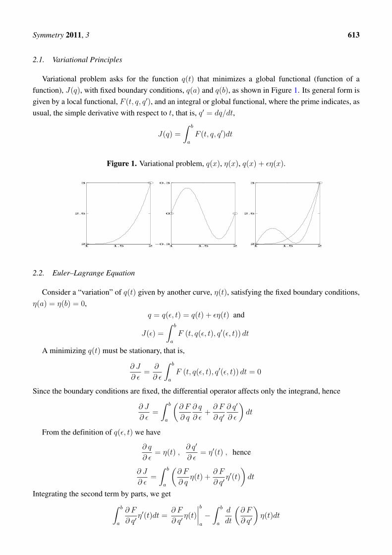
Variational problem asks for the function q(t) that minimizes a global functional (function of afunction), J(q), with fixed boundary conditions, q(a) and q(b), as shown in Figure 1. Its general form isgiven by a local functional, F (t, q, q′), and an integral or global functional, where the prime indicates, asusual, the simple derivative with respect to t, that is, q′ = dq/dt,

J(q) =

∫ b

a

F (t, q, q′)dt

Figure 1. Variational problem, q(x), η(x), q(x) + εη(x).

1 1.5 22

2.5

3

1 1.5 2−0.3

0

0.3

1 1.5 22

2.5

3

2.2. Euler–Lagrange Equation

Consider a “variation” of q(t) given by another curve, η(t), satisfying the fixed boundary conditions,η(a) = η(b) = 0,

q = q(ε, t) = q(t) + εη(t) and

J(ε) =

∫ b

a

F (t, q(ε, t), q′(ε, t)) dt

A minimizing q(t) must be stationary, that is,

∂ J

∂ ε=

∂

∂ ε

∫ b

a

F (t, q(ε, t), q′(ε, t)) dt = 0

Since the boundary conditions are fixed, the differential operator affects only the integrand, hence

∂ J

∂ ε=

∫ b

a

(∂ F

∂ q

∂ q

∂ ε+∂ F

∂ q′∂ q′

∂ ε

)dt

From the definition of q(ε, t) we have

∂ q

∂ ε= η(t) ,

∂ q′

∂ ε= η′(t) , hence

∂ J

∂ ε=

∫ b

a

(∂ F

∂ qη(t) +

∂ F

∂ q′η′(t)

)dt

Integrating the second term by parts, we get∫ b

a

∂ F

∂ q′η′(t)dt =

∂ F

∂ q′η(t)

∣∣∣∣ba

−∫ b

a

d

dt

(∂ F

∂ q′

)η(t)dt


where the first term vanishes, since the extreme points, η(a) = η(b) = 0, are fixed. Hence

∂ J

∂ ε=

∫ b

a

(∂ F

∂ q− d

dt

∂ F

∂ q′

)η(t)dt

Since η(t) is arbitrary and the integral must be zero, the parenthesis in the integrand must be zero. Thisis the Euler–Lagrange equation:

∂ F

∂ q− d

dt

∂ F

∂ q′= 0

If F does not depend explicitly on t, only implicitly through q and q′, Euler–Lagrange equation implies

d

dt

(q′∂ F

∂ q′− F

)= q′′

∂ F

∂ q′+ q′

d

dt

∂ F

∂ q′− ∂ F

∂ t− ∂ F

∂ qq′ − ∂ F

∂ q′q′′ =

−q′(∂ F

∂ q− d

dt

∂ F

∂ q′

)− ∂ F

∂ t= 0 ⇒

(q′∂ F

∂ q′− F

)= const

2.3. Hamilton’s Principle and Classical Mechanics

The Lagrangian of a classical mechanics system specified by generalized vector coordinates q(t),kinetic energy T (q, q′), and potential energy V (q, t), is defined as L(t, q, q′) = T (q, q′)− V (q, t).

Hamilton’s Principle states that, if a classical mechanics system is anchored at initial and final fixedpositions q(a) and q(b), a < b, then the system follows the trajectory that minimizes its physical action,

J(q) =

∫ b

a

L(t, q, q′)dt

defined as the integral of the Lagrangian over time along the system’s trajectory. Noether’s theoremestablishes very general conditions under which the existence of a symmetry in the system, described bythe action of a continuous group in the system, implies the existence of a quantity that remains constantin the system’s evolution, that is, a conservation law, see for example Section 2.7 of [3].

As a first example, consider a Lagrangian L(t, q, q′) that does not depend explicitly of q. This situationreveals a symmetry: The system is invariant by a translation on the coordinate q. From Euler–Lagrangeequation, it follows that the quantity p = ∂ F/∂ q′ is conserved. In the language of classical mechanics,q would be called a cyclic coordinate, while p would be called a generalized moment.

As a second example, consider a Lagrangian that does not depend explicitly on t. In this case,Euler–Lagrange equation implies q′ ∂ L

∂ q′− L = E, where the constant E is interpreted as the system’s

conserved energy. Indeed, if the potential, V (q), is only function of the system position, and the kineticenergy is a quadratic form on the velocities, T =

∑i,j ci,j q

′i q′j , the last equation assumes the familiar

form E = 2T − L = T + V .As a particular instance of the examples above, consider a particle in a plane orbit around a radially

symmetric and time independent potential, L = m2

(r′2 + r2θ′) − V (r). Since the Lagrangian does notdepend explicitly on θ, the system conserves its angular momentum, A, displayed in the next equation.Since the Lagrangian also does not depend explicitly on t, the system conserves its energy, E,

∂ L

∂ q′= mr2q′ = A , T + V =

m

2(r′

2+ r2θ′) + V (r) = E


These two constants of motion, A and E, are in fact a complete set of parameters for the particle’s orbit,that is, these constants fully specify the possible orbits, as becomes clear by combining the last equationsinto the following system of ordinary differential equations,

r′2

=2

m(E − V (r))− m2r2

A, θ′ =

A

mr2

3. Positivism vs. Objective Ontologies

In this section we discuss the ontological status of the constants or conserved quantities that emergefrom Noether’s theorem, such as the energy or angular momentum. In Sections 6 and 7 we are goingto discuss similar formalisms in the realm of mathematical statistics, and will raise similar questionsconcerning the ontological status of parameters in statistical models.

Ontology is the study of oντoς , “of that which is”. Hence, we pose the question: Are these parametersreal, or do they represent or correspond to something real? The commonsense or naıve realism answeris in the affirmative: These parameters correspond to real entities, things that actually exist out there,in the external world or in the environment. These entities can be pointed at and even be preciselymeasured; they are as real as the kitchen sink. The positivist philosophical school strongly dissentsfrom the naıve realism position, claiming that these parameters are nothing but artificial constructs,things that only exist inside the system, model or theory. They are in reality only ghosts. These twoconflicting philosophical positions reappear in a great variety of forms, with many subtle differencesand interesting nuances. We will not venture into the analysis of these fine distinctions, for our maingoal is to overcome this dichotomy with the introduction, in Section 8, of the cognitive constructivismepistemological framework. However, in order to reach this goal, we must analyze several connectionsrelating ontology and the concepts of symmetry and invariance, for these are the keys that can unlockour ontological enigmas.

3.1. Positivism, Subjectivism and Solipsism

According to the positivist school, closely related to the skeptical or solipsist traditions, the primaryphysical quantities must be directly measurable, like (non-relativistic) time, position, etc. In the exampleat hand, the variables of direct interest, corresponding to the primary physical quantities, describe thesystem’s trajectory, giving the time-evolution of the particle’s position, [r(t), θ(t)].

For the positivist school, quantities like A and E have a metaphysical character. The literal meaning ofthe word meta-physical is just beyond-physical, designating entities that are not accessible to our sensesor, in our case, quantities that are not directly measurable. Therefore, from a positivist perspective,metaphysical entities have a very low ontological status, that is, they do not correspond to objects havinga real existence in the world. Rather, they are ghost that only exist inside our formalism.

In the example at hand, E and A constitute a very convenient index system for the collection ofall possible orbits, but that does not grant these quantities any real existence. On the contrary, thesequantities must be considered just as integration constants, useful variables in an intermediate step forthe calculation of the system’s orbits. They can be used as convenient auxiliary variables, generatingsecondary or derived concepts, but that is all that they can ever aspire to be. The physicist Max Born, inpp.49,144,152 of [7], summarizes this position:


Positivism assumes that the only primary statements which are immediately evident are thosedescribing direct sensual impressions. All other statements are indirect, theoretical constructions todescribe in short terms the connections and relations of the primary experiences. Only these have thecharacter of reality. The secondary statements do not correspond to anything real, and have nothing todo with an existing external world; they are conventions invented artificially to arrange and simplify“economically” the flood of sensual impressions.

[The] strictly positivistic standpoint: The only reality is the sense impressions. All the rest are“constructs” of the mind. We are able to predict, with the help of the mathematical apparatus . . . whatthe experimentalist will observe under definite experimental conditions . . . But it is meaningless toask what there is behind the phenomena, waves or particles or what else.

We have before us a standpoint of extreme subjectivism, which may rightly be called “physicalsolipsism”. It is well-known that obstinately held solipsism cannot be refuted by logical argument.This much, however, can be said, that solipsism such as this does not solve but evades the problem.Logical coherence is a purely negative criterion; no system can be accepted without it, but no system isacceptable just because it is logically tenable. The only positive argument in support of this abstracttype of ultra-subjectivism is [that] the belief in the existence of an external world is irrelevant andindeed detrimental to the progress of science.

3.2. Born’s Criticism of Positivism

The gnosiological sense of the word metaphysics has its roots in Aristotelic philosophy: In a nutshell,it designates concepts that enable possible answers to why-questions, that is, metaphysical concepts arethe basis for any possible answer explaining “why” things are the way they do. Hence, metaphysicalconcepts are at the core of metaphorical figures and explanation mechanisms, providing an articulationpoint between the empirical and the hypothetical, a bridge from the rational and the intuitive, a linkbetween calculation and insight. In this role, metaphysical concepts give us access to a “much deeper”level of reality. Without metaphysical concepts, physical reasoning would be downgraded to merelycranking the formalism, either by algebraic manipulation of the symbolic machinery or by sheer numbercrunching. Furthermore, metaphysical concepts are used to express metaphorical figures that constitutethe basis of our communication. These points are addressed by Max Born in pp.144,152 of [7]:

Many physicists have adopted [the positivist] standpoint. I dislike it thoroughly . . . The actualsituation is very different. All great discoveries in experimental physics have been due to theintuition of men who made free use of models, which were for them not products of the imagination,but representatives of real things. How could an experimentalist work and communicate with hiscollaborators and his contemporaries without using models composed of particles, electrons,nucleons, photons, neutrinos, fields and waves, the concepts of which are condemned as irrelevantand futile?

However, there is of course some reason for this extreme standpoint. We have learned that a certaincaution is necessary in using these concepts . . . Modern theories demand a reformulation. This newformulation is slowly evolving, but has probably not reached a final expression.


The final lines of the last quotation address a distinct characteristic of modern science, namely, itsdynamism, the rapid pace of its growth, the creation and reformulation of theories. However, formulatingnew theories implies creating new concepts and, sometimes, abandoning an old one. The frustrationof finding out that some of the traditional good-old “things” do not “exist”, may be followed by thepost-traumatic reaction of denying the existence of anything that is not unequivocally perceived by directsensorial experience. In this setting, the popularity of positivism or subjectivism may be understood as afirst (although clumsy) reaction against naıve realism. We believe that the two extreme epistemologicalpositions of naıve realism and subjective solipsism can be seen as two tentatives of building an ontologybased on a correspondence principle, as opposed to the approach taken in epistemological framework ofcognitive constructivism. We will return to this theme in Section 8.

3.3. Ontology by Invariance and Autonomy

The idea of founding an ontology on invariance properties has its origin in the Erlangen Program ofFelix Klein, [8]. His approach to geometry provided a unified treatment for Euclidean, non-Euclideanand Riemannian geometry, see [9] and [10]. In Klein’s approach, the intrinsic properties of a geometricspace is specified by a set of privileged actions, effected by a discrete or continuous group of possibletransformations. Well-known examples are the rigid translations and rotations of Euclidean geometry,the parallel transport of Riemannian geometry, and so on. Moreover, the essential geometric objects orproperties are characterized as invariants under the specified actions.

Furthermore, invariance suggests self-determination or autonomy: Invariance properties can beinterpreted as stating the irrelevance of peripheral peculiarities. For example, the irrelevance of theparticular coordinate system or reference frame being used (in a well-defined class of equivalence), etc.Hence, invariant objects are perceived to be detached from any idiosyncratic condition, to stand bythemselves, to be autonomous. Max Born, in pp.158,163,104,51 of [7], summarizes this position asapplied to building an ontology for physical sciences:

I think the idea of invariant is the clue to a rational concept of reality, not only in physics butin every aspect of the world. The theory of transformation groups and their invariants is a wellestablished part of mathematics. Already in 1872 the great mathematician Felix Klein discussed inhis famous ‘Erlanger Program’ the classification of geometry according to this point of view; thetheory of relativity can be regarded as an extension of this program to the four-dimensional geometryof space-time. The question of reality in regard to gross matter has from this standpoint a clear andsimple answer.

Thus we apply analysis to construct what is permanent in the flux of phenomena, the invariants.Invariants are the concepts of which science speaks in the same way as ordinary language speaks of“things”, and which it provides with names as if they were ordinary things.

The words denoting things are applied to permanent features of observation orobservational invariants.

The invariants of [a] theory have the right to be considered as representations ofobjects in the real world. The only difference between them and the objects of everyday life is that the


latter are constructed by the unconscious mind, whereas the objects of science are constructed byconscious thinking.

In the next sections we will analyze some formalisms for dealing with symmetry and invariance inBayesian statistics, their traditional subjectivist interpretations, and alternative ontological or objectiveinterpretations based on the concepts of symmetry and invariance.

4. Bayesian Statistics

A standard model of (parametric) Bayesian statistics concerns an observed (vector) random variable,x, in the sampling space, X , that has a sampling distribution with a specified functional form, p(x | θ),indexed by the (vector) parameter, θ, in the parameter space, Θ. This same functional form, regardedas a function of the free variable θ with a fixed argument x, is the model’s likelihood function. Infrequentist or classical statistics, one is allowed to use probability calculus in the sample space, butstrictly forbidden to do so in the parameter space, that is, x is to be considered as a random variable,while θ is not to be regarded as random in any way. In frequentist statistics, θ should be taken as a “fixedbut unknown quantity”.

In the Bayesian context, the parameter θ is regarded as a latent (non-observed) random variable.Hence, the same formalism used to express credibility or (un)certainty, namely, probability theory, isused in both the sample and the parameter space. Accordingly, the joint probability distribution, p(x, θ)should summarize all the information available in a statistical model. Following the rules of probabilitycalculus, the model’s joint distribution of x and θ can be factorized either as the likelihood function ofthe parameter given the observation times the prior distribution on θ, or as the posterior density of theparameter times the observation’s marginal density,

p(x, θ) = p(x | θ)p(θ) = p(θ |x)p(x)

The prior probability distribution p0(θ) represents the initial information available about theparameter. In this setting, a predictive distribution for the observed random variable, x, isrepresented by a mixture (or superposition) of stochastic processes, all of them with the functional form ofthe sampling distribution, according to the prior mixing (or weights) distribution,

p(x) =

∫θ

p(x | θ)p0(θ)dθ

If we now observe a single event, x, it follows from the factorizations of the joint distribution abovethat the posterior probability distribution of θ, representing the available information about the parameterafter the observation, is given by

p1(θ) ∝ p(x | θ)p0(θ)

In order to replace the “proportional to” symbol, ∝, by an equality, it is necessary to divide the righthand side by the normalization constant, c1 =

∫θp(x | θ)p0(θ)dθ. This is the Bayes rule, giving the

(inverse) probability of the parameter given the data. That is the basic learning mechanism of Bayesianstatistics. Computing normalization constants is often difficult or cumbersome. Hence, especially inlarge models, it is customary to work with unnormalized densities or potentials as long as possible


in the intermediate calculations, computing only the final normalization constants. It is interesting toobserve that the joint distribution function, taken with fixed x and free argument θ, is a potential for theposterior distribution.

Bayesian learning is a potentially recursive process, where the posterior distribution after alearning step becomes the prior distribution for the next step. Assuming that the observations are i.i.d.(independent and identically distributed) the posterior distribution after n observations, x(1), . . . x(n),becomes,

pn(θ) ∝ p(x(n) | θ)pn−1(θ) ∝∏n

i=ip(x(i) | θ)p0(θ)

If possible, it is very convenient to use a conjugate prior, that is, a mixing distribution whose functionalform is invariant by the Bayes operation in the statistical model at hand. For example, the conjugatepriors for the Normal and Multivariate models are, respectively, Wishart and the Dirichlet distributions.The explicit form of these distributions is given in the next sections.

In the next two subsections we further discuss the dynamics of the Bayesian learning process, that is,we present some rationale for choosing the prior distribution used to start the learning process, and someconvergence theorems for the posterior as the number observations increases.

4.1. Fisher’s Metric and Jeffreys’ Prior

The Fisher information matrix, J(θ), is defined as minus the expected Hessian of the log-likelihood.The Fisher information matrix can also be written as the covariance matrix of for the gradient of thesame likelihood, i.e.,

J(θ) ≡ −E∂ 2 log p(x | θ)

∂ θ2= E

(∂ log p(x | θ)

∂ θ

∂ log p(x | θ)∂ θ

)The physicist Harold Jeffreys [11] used the Fisher’s metric to define a class of prior distributions

proportional to the determinant of the information matrix,

p(θ) ∝ |J (θ)|1/2

Jeffreys’ priors are geometric objects in the sense of being invariant by a continuous and differentiablechange of coordinates, η = f(θ), in the parameter space, see pp. 41–54 of [12]. That is:

J(θ) =

[∂ η

∂ θ

]J(η)

[∂ η

∂ θ

]′, hence

|J (θ)|1/2 dθ =

∣∣∣∣∂ η∂ θ∣∣∣∣ |J (η)|1/2 = |J (η)|1/2 dη

It is important to realize that the argument of transformation-invariance used in the derivation ofJeffrey’s priors is quite distinct from the argument of symmetry-invariance relative to the action of agiven group in the system used in Noether’s theorem. Nevertheless, in Sections 5, 6 and 7 this latertype of argument will be used to derive parametric families of sampling distributions for which, inturn, Jeffrey’s priors offer a coherent starting point or ground state in the Bayesian inferential process.Moreover, transformation-invariance is, in its own right, an important property intimately related to ourleitmotif of ontology by invariance and autonomy, as further discussed in Sections 8 and 9.


Example (multinomial distribution):

p(y | θ) = n!∏m

i=1θxii

/∏m

i=1xi! , θm = 1−

∑m−1

i=1θi , xm = n−

∑m−1

i=1xi

L = log p(x | θ) =∑m

i=1xi log θi

∂ 2L

(∂ θi)2= −xi

θ2i

+xmθ2m

,∂ 2L

∂ θi∂ θj= −xm

θ2m

, i, j = 1 . . .m− 1

−E∂ 2L

(∂ θi)2=n

θi+

n

θm, −E

∂ 2L

∂ θi∂ θj=

n

θm

|J(θ)| = (θ1θ2 . . . θm)−1 , p(θ) ∝ (θ1θ2 . . . θm)−1/2

p(θ |x) ∝ θx1−1/21 θ

x2−1/22 . . . θxm−1/2

m

Hence, in the multinomial example, Jeffreys’ prior “discounts” half an observation of each kind, whilethe flat prior discounts none.

4.2. Posterior Convergence

In this section we briefly state two asymptotic results that are fundamental to Bayesian statistics. Fora detailed, intuitive and very understandable discussion, see Appendix B of [13].

Theorem 4.1 (Posterior Consistency for Discrete Parameters). Consider a model where f(θ) is theprior in a discrete (vector) parameter space, Θ = {θ(1), θ(2), . . .}, X = [x(1), . . . x(n)] is a series ofobservations, and the posterior is given by

f(θ(k) |X) ∝ f(θ(k)) p(X | θ(k)) = f(θ(k))∏n

i=1p(x(i) | θ(k))

Further, assume that in this model there is a single value for the vector parameter, θ(0), that givesthe best approximation for the “true” predictive distribution g(x) (in the sense that it minimizes theinformation divergence, as defined in Section 7). Then,

limn→∞

f(θ(k) |X) = δ(θ(k), θ(0))

We can extend this result to continuous parameter spaces, assuming several regularity conditions, likecontinuity, differentiability, and having the argument θ(0) as a interior point of Θ with the appropriatetopology. In such a context, we can state that, given a pre-established small neighborhood around θ(0),like C(θ(0), ε) the cube of side size ε centered at θ(0), this neighborhood concentrates almost all mass off(θ |X), as the number of observations grows to infinity. Under the same regularity conditions, we alsohave that Maximum a Posteriori estimator is a consistent estimator, i.e., θ → θ(0).

The next result states the convergence in distribution of the posterior to a Normal distribution, usingthe Fisher information matrix as defined in the last subsection, see Appendix B of [13].

Theorem 4.2 (Posterior Normal Approximation). The posterior distribution converges to a Normaldistribution with mean θ(0) and precision nJ(θ(0)).


4.3. Subjective Coherence vs. Objective Priors

The invariance properties of Jeffreys’ priors entail objective interpretations that may be suggested inanalogy with Noether’s theorem. In pp. 132–133 of [14], we find some further explanations for themeaning of Weyl’s opening quote in this paper:

We found that objectivity means invariance with respect to the group of automorphisms . . . Thisis what Felix Klein called a ‘geometry’ in the abstract sense. A geometry, Klein said, is defined bya group of transformations, and investigates everything that is invariant under the transformations ofthis given group.

Under appropriate regularity conditions, the information geometry is defined by the metric in theparameter space given by the Fisher information matrix, that is, the geometric length of a curve iscomputed integrating the differential form dl2 = dθ′J(θ)dθ, see [15–17]. Hence, in analogy with Klein’sErlangen Program, Jeffreys’ priors can be interpreted as giving the underlying geometry of the parameterspace. In this role, Jeffreys’ priors provide reference metrics for the parameter space of statistical models,metrics that we so often take for granted and use for a great variety of purposes without further thought orconsideration. Under the objective perspective, the posterior convergence theorem characterizes “true”parameter values as fixed points of the learning process, that is, as (stochastic) invariants. Naturally, allthese interpretations have a strong objective character.

However, subjective interpretations of the results presented in this section are also possible. Underthe subjectivist perspective, Jeffreys’ prior can be understood as coherence conditions for the subject’sopinion. For a subjectivist, invariance by reparameterization is only a consistency condition on rationalbut personal prior beliefs. Even convergence results can be re-interpreted as leading not to to any kindof objectivity, but to inter-subjectivity, that is, as leading, in due time, to the mutual agreement of severalsolipsist agents. However, perhaps the best justification or the most powerful defense for the subjectivistposition was presented by Bruno de Finetti, the undisputed champion of the subjectivist position. Inthe next section we review de Finetti’s theorem and its original interpretation. These considerations, notsurprisingly, are based on yet another symmetry relation, namely, exchangeability.

5. Exchangeability and De Finetti Theorems

In Section 4 we derived several results of Bayesian statistics assuming that observations arei.i.d. random variables, Nevertheless, the i.i.d. hypothesis has a strong “objectivist” flavor. DeFinetti’s theorem, [18,19], allows us to replace the i.i.d. hypothesis by a symmetry condition,namely, exchangeability.

A finite sequence of n random (vector) variables, y(1), y(2), . . . y(n) is (finitely) exchangeable if thejoint distribution of these random variables is permutation-symmetric, that is, if, for any permutation πin {1, 2, . . . n},

p(y(1), y(2), . . . y(n)) = p(yπ(1), yπ(2), . . . yπ(n))

An infinite sequence of random variables is infinitely exchangeable if any of its finite subsequencesis exchangeable.


Bruno de Finetti’s original exchangeability theorem states that, for an infinite exchangeable sequenceof (scalar) Boolean random variables, partial joint probability distributions can always be represented asa mixture on the parameter space of a product of Bernoulli distributions,

p(y1, . . . yn) =

∫ 1

0

∏n

i=1θyi(1− θ)1−yi q(θ)dθ =

∫ 1

0

θxn(1− θ)1−xn q(θ)dθ

the probability distributions of the partial sums, xn =∑n

i=1 yi, can always be represented as thecorresponding mixture on the parameter of binomial distributions,

f(xn) =

(n

xn

)∫ 1

0

θxn(1− θ)1−xn g(θ)dθ

and the mixing cumulative distribution, G(θ), is the limit cumulative distribution for thepartial frequencies,

Gn(θ) = Pr (xn/n ≤ θ)

The statement above assumes that there is a limit density, g(θ); otherwise one has to employ the abstractlimit probability measure, dG(θ). For a simple and intuitive proof, see Section VII.1.4 of [20]. Feller’sproof follows some of the same arguments used by de Finetti, including some interesting demonstrationtechniques based on the theory of difference equations, see [18,19,21]. For a short and elegant proof thatrelies on measure theoretic analysis, see [22]. For several extensions of de Finetti’s theorem, see [23,24].

From simple characterization theorems, see [25], it is immediate to extend de Finetti’s theorem fromthe Binomial to the Multinomial case. Arguments of analysis, see Chapter 4 of [26] or Section VII.12of [27], allow us to further extend de Finetti’s theorem to obtain a general representation theorem forfinite subsequences of an infinitely exchangeable sequence of real-valued random variables. Assumingthat ordinary densities can replace the more abstract probability measures, the general form of the jointprobability distribution for a finite set of (observed) random variables, x1, . . . xn, can be representedby the product of a parameterized density for individual observations mixed by a density on the(latent) parameter,

p(x(1), . . . x(n)) =

∫Θ

∏n

i=1p(x(i) | θ)q(θ)dθ

If these probability models are subject to additional constraints, like the symmetry conditions consideredin next sections, the general representation takes the form of a mixture in the corresponding family ofinvariant distributions.

5.1. De Finetti’s Subjectivism

Bruno de Finetti is the founder of modern Bayesian statistics, and an outspoken advocate of extremesubjectivism. In his lecture—Exchangeability, Induction and “Unknown” Probabilities—Chapter 8of [28], de Finetti offers a synthesis of his interpretation of probability as subjective uncertainty in thecontext of the theorem presented in the last section:

Every time that probability is given by a mixture of hypotheses, with independence holding foreach of them respectively, it is possible to characterize the inductive relevance that results on the


basis of [the mixture] equation in terms of exchangeability . . . [This] shows how the concept ofexchangeability is necessary in order to express in a meaningful way what is usually referred to as“independence with constant but unknown probability”. This expression is not correct because in fact(a) there is no independence; (b) the probability is not constant because the composition of the urnbeing unknown, after learning the outcome of the draws, the probability of the various compositionsis subject to variation.

Hence, according to de Finetti, the “objective” i.i.d. condition is a mirage, a displaced reflection“outside” of a more fundamental symmetry condition “inside”, namely, exchangeability. Naturally, forde Finetti, exchangeability is on the eyes of the beholder, expressing his or her own explicit or implicitopinions on how observational data should be correctly handled.

Irving John Good was another leading figure of the early days of the Bayesian revival movement.Contrary to de Finetti, Good has always been aware of the dangers of an extreme subjectivist position.Some of his conclusions seem to echo Born’s arguments presented in Section 1, see for example, RandomThoughts about Randomness, p. 93 in Chapter 8 of [29].

Some of you might have expected me, as a confirmed Bayesian, to restrict the meaning of the word‘probability’ to subjective (personal) probability. That I have not done so is because I tend to believethat physical [objective] probability exists and is in any case a useful concept... The philosophicalimpact of de Finetti’s theorem is that it supports the view that solipsism cannot be logically disproved.Perhaps it is the mathematical theorem with most potential philosophical impact.

In Sections 6 and 7, we shall widen the scope of our discussion, presenting probability distributionsderived from symmetry conditions far more general than exchangeability. Some of these examples areof great historical importance. However, in contrast to de Finetti’s theorem, some of these resultsseem to favor objective interpretations. As planned in the introduction, we will continue to explorethe importance of symmetry arguments in the realism-subjectivism debate. Nevertheless, the increasingpower and sophistication of the available symmetry arguments seem to have the effect of generating evermore violent oscillations or inducing an even greater polarization between the two alternatives in therealism-subjectivism dilemma. Sections 6 and 7 are the last steps leading to the presentation, in Section 8,of the cognitive constructivism epistemological framework that, as promised in the introduction, will beable to solve (many aspects of) the ongoing ontological conundrum.

6. Simple Symmetric Probability Distributions

Sections 6 and 7 present important results linking symmetry constraints and the functional form ofprobability distributions. We follow the very simple approach to functional equations of probabilitydistributions in [30]. For related but more general and sophisticated approaches, see [31–33].

6.1. Cauchy’s Functional Equations

In this subsection we introduce the additive and multiplicative forms of Cauchy functional equation,since this functional equation will be used several times in the sequel.


Cauchy’s additive functional equation has the form

f(x+ y) = f(x) + f(y)

The following argument from Cauchy (1821) shows that a continuous solution of this functional equationmust have the form

f(x) = cx

Repeating the sum of the same argument, x, n times, we must have f(nx) = nf(x). If x = (m/n)t,then nx = mt and

nf(x) = f(nx) = f(mt) = mf(t) , hence

f(mnt)

=m

nf(t)

taking c = f(1), and x = m/n, it follows that f(x) = cx, over the rationals, x ∈ IQ. From the continuitycondition for f(x), the last result must also be valid over the reals, x ∈ R. Q.E.D.

Cauchy’s multiplicative functional equation has the form

f(x+ y) = f(x)f(y) , ∀x, y > 0 , f(x) ≥ 0

The trivial solution of this equation is f(x) ≡ 0. Assuming f(x) > 0, we take the logarithm, reducingthe multiplicative equation to the additive equation,

ln f(x+ y) = ln f(x) + ln f(y) , hence

ln f(x) = cx , or f(x) = exp(cx)

6.2. Radial Symmetry and the Gaussian Distribution

John Herschel [34] gave the following derivation of the Gaussian or Normal distribution, concerningthe distribution of errors in astronomical measurements, see also [35].

A few years later, James Clerk Maxwell used the same arguments to derive the functional form of theprobability distribution of molecular velocities in statistical physics. The derivation follows three simplesteps, based on arguments of (1) independence; (2) radial symmetry; and (3) normalization. For the sakeof simplicity, we give the derivation using a two dimensional Cartesian coordinate system, x = [x1, x2].

Axial independence (a.k.a. orthogonality condition): Measurements on orthogonal axes should beindependent. Hence, the joint distribution should be decomposed in product form,

f(x) = f(x1)f(x2)

Radial symmetry (a.k.a. isotropy condition): Measurement errors should not depend on the currentorientation of the coordinate system. This step uses the exponential solution to Cauchy multiplicativefunctional equation.

f(x) = f(x1)f(x2) = f(x21 + x2

2)⇒ f(x) ∝ exp(x21 + x2

2) = exp(||x||2)

Normalization: The probability density must integrate to unity.∫f(x)dx1dx2 = 1⇒ f(x) =

a

πexp(−a||x||2) , a > 0


In the next section, we give a second derivation of this functional form based on the MaxEntformalism, given more general constraints on the first and second statistical moments, that is, theexpectation vector and covariance matrix.

6.3. Homogeneous Discrete Markov Processes

We seek the general form of a homogeneous discrete Markov process. Let wk(t), for t ≥ 0, be theprobability of occurrence of exactly k events. Let us also assume the following hypotheses:

Time Locality: If t1 ≤ t2 ≤ t3 ≤ t4, then the number of events in [t1, t2] is independent of the numberof events in [t3, t4].

Time Homogeneity: The distribution for the number of events occurring in [t1, t2] depends only onthe interval length, t = t2 − t1.

From time locality and homogeneity, we can decompose the occurrence of no (zero) events in [0, t+

u] as,w0(t+ u) = w0(t)w0(u)

Hence, w0(t) must obey Cauchy’s functional equation, and

w0(t) = exp(ct) = exp(−λt)

Since w0(t) is a probability distribution, w0(t) ≤ 1, and λ > 0.Hence, v(t) = 1 − w0(t) = 1 − exp(−λt), the probability of one or more events occurring before

t > 0, must be the familiar exponential distribution.For k ≥ 1 occurrences before t+ u, the general decomposition relation is

wn(t+ u) =n∑k=0

wk(t)wn−k(u)

Theorem 6.1 (Renyi–Aczel). The Poisson distribution,

wk(t) = e−λt(λt)k/k!

is the (non-trivial) solution of this system of functional equations under the rarity condition: Theprobability that an event occurs in a short time at least once is approximately equal to the probability thatit occurs exactly once, that is, the probability of simultaneous occurrences is zero. The general solutionhas the form of a mixture of Poisson processes, each one counting bursts of a fixed number of events.For the proof, by induction, see Section 2.1–2.3 in [30].

Pereira and Stern [25] present the characterization of the Multinomial by the Poisson distribution,and vice versa. These characterizations allow us to interpret the exchangeability symmetry characterizinga Multinomial processes in terms of the time homogeneity symmetry and superposition principlecharacterizing corresponding Poisson counting processes, and vice versa. From a strict predictiviststandpoint, it can be observed, our analogy between de Finetti’s and Renyi–Aczel theorems is not fullycomplete, because an exogenous (to the characterization) mixing distribution on the Poisson parameterhas to be integrated into the Bayesian inferential model. In order to present our analogy argument infull strength, the straight i.i.d. hypothesis for non-overlapping same-length intervals in Renyi-Aczel


theorem, as stated in Section 2.3.6 of [30], should be replaced by a weaker conditional i.i.d. hypothesis,given the asymptotic frequency rate of the stochastic process. A direct characterization of the mixedPoisson process can be found in Proposition 1.28 at p.66 of [36].

7. Minimum Information or MaxEnt Principle

Section 2 presented Noether’s theorem that, based on the minimum action principle and the system’sinvariance under a group action produces an invariant (physical) quantity. This section presents theMaximum Entropy (MaxEnt) argument to derive the functional form of an invariant distribution. It ispossible to derive the functional form of many of the most probability distributions used in statisticalmodels, see [37]. We also present Bregman’s algorithm as simple and elegant way to compute finiteMaxEnt distributions even when no closed analytical form is available. The formulation of Bregman’salgorithm also provides a useful tool for quickly validating the analytic form of many MaxEnt solutions.Many readers with a good background in probability and statistics will be well-acquainted with thismaterial and may rather skip the following examples and derivations. These are kept as simple aspossible, in order to make them easily accessible to readers from different backgrounds. We also hopethat this approach will help them to understand and recognize the similarities between the techniquespresented in this section and analogous techniques presented in Sections 2.

The formal similarities between the minimum action and MaxEnt frameworks imply that all thepositivist and anti-positivist positions analyzed in Section 3 can be carried over to the realm of statistics.In particular, all the heated debates concerning the reality of parameters, or what they represent, canbe restated, almost ipsis litteris, in the context of statistical models. Furthermore, the same formalsimilarities will allow many epistemological arguments used to introduce the cognitive constructivismframework to be carried from the domain of physics to statistics, and vice versa.

7.1. Maximum Entropy under Constraints

The origins of the entropy concept lay in the fields of thermodynamics and statistical physics, butits applications have extended far and wide to many other phenomena, physical or not. The entropyof a probability distribution, H(p(x)), is a measure of uncertainty (or impurity, confusion) in a systemwhose states, x ∈ X , have p(x) as probability distribution. For detailed analysis and further references,see [38–40] and Appendix E of [41]. For the sake of simplicity, we present most of the followingdiscussion in the context of a finite system, with states spanned by an indexed i ∈ {1, 2, . . . n}.

The Boltzmann–Gibbs–Shannon measure of entropy is defined as

Hn(p) = −In(p) = −∑n

i=1pi log(pi) = −Ei log(pi) , 0 log(0) ≡ 0

The opposite of the entropy, I(p) = −H(p), the negentropy, is a measure of information available aboutthe system.

Shannon’s inequality, a theorem that follows directly from the definition of entropy, can be statedas follows: If p and q are two distributions over a system with n possible states, and qi 6= 0, then theinformation divergence of p relative to q, In(p, q), is positive, except if p = q, when it is null,

In(p, q) ≡∑n

i=1pi log

(piqi

), In(p, q) ≥ 0 , In(p, q) = 0⇒ p = q


Shannon’s inequality motivates the use of the information divergence as a measure of (non-symmetric)“distance” between distributions. In statistical sciences, this measure is known as the Kullback–Leiblerdistance. The denominations directed divergence or cross information are used in Engineering.

Given a prior distribution, q, we would like to find a vector p that minimizes the informationdivergence In(p, q), where p is under the constraint of being a probability distribution, and maybe alsounder additional constraints over the expectation of functions taking values on the system’s states. In thespecification of the constraints, A is an (m− 1)× n real matrix, and the problem is formulated as

p∗ ∈ arg min In(p, q) , p ≥ 0 | 1′p = 1 and Ap = b

The solution p∗ is the minimum information divergence distribution, relative to q, given the constraints{A, b}. We can write the probability normalization constraint as a generic linear constraint, including1 and 1 as the m-th (or 0-th) rows of matrix A and vector b. By doing so, we do not need to keep anydistinction between the normalization and the other constraints. The operators � e � indicate the point(element) wise product and division between matrices of same dimension.

The Lagrangian function of this optimization problem and its derivatives are:

L(p, w) = p′ log(p� q) + w′(b− Ap)

∂ L

∂ pi= log(pi/qi) + 1− w′A•,i ,

∂ L

∂ wk= bk − Ak,• p

Equating the n+m derivatives to zero, we have a system with n+m unknowns and equations, givingviability and optimality conditions (VOCs) for the problem:

pi = qi exp (w′A•,i − 1) or p = q � exp ((w′A)′ − 1)

Ak,• p = bk , p ≥ 0

We can further replace the unknown probabilities, pi, writing the VOCs only on w, the dual variables(Lagrange multipliers),

hk(w) ≡ Ak,• (q � exp ((w′A)′ − 1))− bk = 0

In the case of finite systems, the last form of the VOCs motivates the use of iterative algorithms ofGauss–Seidel type, solving the problem by cyclic iteration. In this type of algorithm, one cyclically “fits”one equation of the system, for the current value of the other variables. For a detailed analysis of thistype of algorithm, see [42–46].

Bregman’s Algorithm:Initialization: Take t = 0, w(t) ∈ Rm, and

p(t)i = qi exp

(w(t)′A•,i − 1

)Iteration step: for t = 1, 2, . . ., Take

k = (t mod m) and ν |ϕ(ν) = 0 , where


w(t+1) =[w

(t)1 , . . . w

(t)k−1, w

(t)k + ν, w

(t)k+1, . . . w

(t)m

]′p

(t+1)i = qi exp(w(t+1)′A•,i − 1) = p

(t)i exp(νAi,k)

ϕ(ν) = Ak,• p(t+1) − bk

From our discussion of entropy optimization under linear constraints, it should be clear that theminimum information divergence distribution for a system under constraints on the expectation offunctions taking values on the system’s states,

Ep(x)ak(x) =

∫ak(x)p(x)dx = bk

(including the normalization constraint, a0 = 1, b0 = 1) has the form

p(x) = q(x) exp (−θ0 − θ1 a1(x)− θ2 a2(x) . . .)

Note that we took θ0 = −(w0 − 1), θk = −wk, and we have also indexed the state i by variable x,so to write the last equation in the standard form used in the statistical literature. Hence, this form isa convenient way to check that several distributions commonly used in statistics can be interpreted asminimum information (or MaxEnt) densities (relative to the uniform distribution, if not otherwise stated)given some constraints over the expected value of state functions. For example:

- The Binomial distribution is characterized as the distribution of maximum entropy for i ∈{1 . . . n}, given the expected value of the mean, relative to the combinatorial prior C(n, i).- The Normal distribution is characterized as the distribution of maximum entropy on Rn, given the

expected values of its first and second moments, i.e., mean vector and covariance matrix.- The Wishart distribution:

f(S | ν, V ) ≡ c(ν, V ) exp

(ν − d− 1

2log(det(S))−

∑i,jVi,jSi,j

)is characterized as the distribution of maximum entropy in the support S > 0, given the expectedvalue of the elements and log-determinant of matrix S. That is, writing Γ′ for the digamma function,

E(Si,j) = Vi,j , E(log(det(S))) =∑d

k=1Γ′(ν − k + 1

2

)- The Dirichlet distribution

f(x | θ) = c(θ) exp(∑m

k=1(θk − 1) log(xk)

)is characterized as the distribution of maximum entropy in the simplex support, x ≥ 0 | 1′x = 1, giventhe expected values of the log-coordinates, E(log(xk)).

For the Multinomial distribution, the mean vector represents expected frequency rates, and thecombinatorial prior represents the equiprobability condition. The Multinomial distribution is only afunction of accumulated counts, it is not dependent on the particular order of the outcomes. Hence itrepresents exchangeable events, generalizing the Binomial case examined in Section 5.


For the Normal distribution, the mean represents a translation vector, and the coefficients ofthe correlation matrix represent rotation angles. Translations and rotations constitute the actiongroup defining Euclidean geometry. In particular, Herschel’s isotropy and orthogonality conditions, seeSection 6.2, are expressed by the zero mean vector and (multiples of) the identity correlation matrix. Fora general discussion for symmetry characterizations of the Normal distribution, see Section 8.2 of [32].

The Dirichlet and the Wishart distribution can be characterized as conjugate andtransformation-invariant priors for the first two distributions, or as MaxEnt distributions in theiron right. Dirichlet-Multinomial and Normal-Wishart models, and many of its variations, like discreteBayesian networks, regression, factor analysis, generalized linear models, and combinations of theabove, known as finite mixture models, encompass the most widely used classes of statistical models.This is due to the formal convenience for mathematical manipulation offered by these models, and alsoby the importance (in the target application) of the symmetries encoded by these models. The nextsection should help to clarify this last statement.

8. Cognitive Constructivism

In the preceding sections, we have discussed several forms of invariance found in statistical models.However, a fundamental epistemological inquiry concerns whether these invariances concern: (a) theobserver; (b) the observed phenomena an sich (in itself); or (c) the observation process. Thesethree possibilities are related to the epistemological frameworks of (a) subjectivism, skepticism,solipsism, etc.; (b) naıve or dogmatic forms of realism; (c) cognitive constructivism. Previous sectionsdiscussed some aspects of the first two epistemological frameworks. The last sections make additionalconsiderations about these two frameworks and also introduce a third option, Cognitive Constructivism,or Cog-Con.

8.1. Objects as Eigen-Solutions

The Cog-Con framework rests upon Heinz von Foerster’s metaphor of Objects as tokens foreigen-solutions, the key to Cog-Con ontology and metaphysics. The recursive nature of a learningsystem interacting with its environment produces recurrent states or stable solutions. Under appropriateconditions, such a (learned or known) solution, if presented to the system, will regenerate itself asa fixed point, an equilibrium or homeostatic state, etc. These are called eigen-values, eigen-vectors,eigen-functions, eigen-behaviors or, in general, eigen-solutions. The circular or cyclic characteristic ofrecursive processes and their eigen (auto, equilibrium, fixed, homeostatic, invariant, recurrent, recursive)states are investigated by von Foerster in [47,48]. The concept of eigen-solution is the key to distinguishspecific objects in the cognitive domain of a learning system. Objects are “tokens for eigen-solutions”.(A soccer ball is something that interacts with a human in the exact way it is supposed to do for playingsoccer.) Eigen-solutions can also be tagged or labeled by words, and these words can be articulated inlanguage. Of course, the articulation rules defined for a given language, its grammar and semantics, onlymake the language useful if they somehow correspond to the composition rules for the objects the wordsstand for.


Moreover, von Foerster establishes four essential attributes of eigen-solutions: Eigen-values areontologically discrete, stable, separable and composable. It is important to realize that, in the sequel,the term “discrete”, used by von Foerster to qualify eigen-solutions in general, should be replaced,depending on the specific context, by terms such as lower-dimensional, precise, sharp, singular etc.In several well-known examples in exact sciences, these four essential properties lead to the concept ofbasis, basis of a finite vector space, like in linear algebra, basis of a Hilbert space, like in Fourier orWavelet analysis, or more abstract settings, like basis for matroid structure, generators for an algebraicgroup, etc. Nevertheless, the concept of eigen-solution and its four essential properties is so importantin the Cog-Con framework that it is used as a fundamental metaphor in far more general—and notnecessarily formalized—contexts. For detailed interpretations of the of these four essential attributes oneigen-solutions in the context of Bayesian learning systems, see [41,49–52].

8.2. Semantics by Construction and by Correspondence

In this subsection we further investigate some consequences of the Cog-Con perspective on objectsand their representation in language, contrasting it with more traditional approaches, based on dyadiccuts and subsequent correspondences. Correspondence approaches start by making a distinction thatcuts the world in two, and then choose or decide if objects are correctly placed “in here” or “out there”:Are they internal concepts in a given system or are they external entities in the environment? Do theybelong to the “subjective” or “upper” world of the mind, spirit, intuitive thought etc., or do they belongto “reality” or “lower” world of the body, matter, etc.?

The predetermined cut splitting the world in two also suggests two natural alternative ways to travelthe epistemological path: Either the correct ideas above are those corresponding to the “reality” below,or the correct things below are those corresponding to the “good” ideas above, etc. The existence of trueand static correspondence principle is a necessary pre-requisite, but there are different ways to establishthe connection, or to learn it (or to remember it). An empiricist diligently observes the world, expectingto develop convenient tools and technology that can, in turn, be used to climb the track of scientificdiscovery. A dogmatic idealist works hard at his metaphysical doctrine, in order to secure a good spot atthe top, expecting to have an easy ride sliding down the trail of knowledge.

The dyadic correspondence approach is simple and robust. It can be readily adapted to many differentsituations and purposes. It also has attractive didactic qualities, being easy to understand and to teach.The dyadic correspondence approach has low entrance fees and low maintenance costs, as long as oneunderstands that the assumption of a predetermined correspondence makes the whole system essentiallystatic. Its major weakness relates to this rigidity. It is not easy to consider new hypothesis or originalconcepts, and even harder to handle the refutation or the dismissal of previously accepted ones. Newworld orders always need to be, at least conceptually, proven afresh or build up from scratch.

In Cognitive Constructivism, language can be seen as a third pole in the epistemological framework,a third element that can play the role of a buffer, moderating or mitigating the interaction of systemand environment, the relation of theory and experiment, etc. After all, it is only in language that it ispossible to enunciate statements, which can then be judged for truthfulness or falsehood. Moreover,language gives us a shelf to place our objects (representations of eigen-solutions), a cabinet to storethese (symbolic) tokens. Even if the notion of object correspondence, to either purely internal concepts


to a given system or to strictly external entities in the environment, is inconsistent with the Cog-Conframework, this framework is perfectly compatible with having objects re-presented as symbols in oneor several languages. This view is very convenient and can be very useful, as long as we are not carriedaway, and start attributing to language magic powers capable of creating ex nihilo the world we live in.As naıve as this may seem, this is a fatal mistake made by some philosophers in the radical constructivistmovement, see [41].

The Cog-Con approach requires, from the start, a more sophisticated construction, but it shouldcompensate this trouble with the advantage of being more resilient. Among our goals is escaping thedilemmas inherent to predetermined correspondence approaches, allowing more flexibility, providingdynamic strength and stability. In this way, finding better objects, representing sharper, stabler, easier tocompose, or more generally valid eigen-solutions (or even better representations for these objects in thecontext of a given system) does not automatically imply the obliteration of the old ones. Old concepts ornotations can be replaced by better ones, without the need of ever being categorically discredited. Hence,theories have more room to continuously grow and adapt, while a concept at one time abandoned maybe recycled if its (re)use is convenient at a later opportunity. In this way, the Cog-Con epistemologicalframework naturally accommodates dynamic concepts, change of hypotheses and evolution of theories,all so characteristic of modern science.

9. Conclusions and Further Research

When Bayesian statistical models are examined in the Cog-Con framework, the role played bythe model’s parameters becomes clear: They are (converging to stochastic) eigen-solutions of theBayesian learning process of information acquisition by the incorporation of observational data. Theseeigen-solutions are characterized by several important invariance properties including asymptotic,symmetry and transformational aspects. All these distinct invariance properties are interrelated by thestructure of the statistical model and, in the spirit of Herman Weyl’s opening quote in this paper, mutuallysupport the notion of emerging eigen-solutions as autonomous ontological objects. The precision aspectof the quality of such an eigen-solution can be evaluated by its current posterior density and suchan evaluation can, in turn, be used to access its objectivity. Similarly, we can access the objectivetruthfulness of more general hypotheses, stated as equations on the parameters. The Full BayesianSignificance Test was designed having this very purpose in mind, including the evaluation of otheraspects of eigen-solutions represented by statistical hypotheses, like their stability and compositionality,see [49,53–55].

Frequentist statistics categorically forbids probabilistic statements in the parameter space. DeFinettian subjectivist interpretation of Bayesian statistics “justifies” the use of prior and posteriordistributions for the parameters, but their role is to be used as nothing more than integration variables inthe process of computing predictive distributions. In a very positivist spirit, like any other non-directlyobservable or latent quantity, parameters are labeled as meta-physical entities, and given a very lowontological status. Finally, in the Cog-Con interpretation of Bayesian statistics, parameters can taketheir rightful place on the center stage of the inferential process. They are not just auxiliary variables,but legitimate objects of knowledge that can be properly used in true bearing statements. We claim


that the last situation corresponds to what a scientist naturally finds, needs and wants in the practice ofempirical science.

Ontological frameworks based on correspondence semantics seem to be particularly inappropriate inquantum mechanics. We believe that many of the arguments and ideas presented in this paper can bere-presented, even more emphatically, for statistical models concerning experimental measurements inthis realm. The formal analogies between the invariance arguments and their use in statistics and physicsis even stronger in quantum mechanics than in the case of classical physics, see [56–60]. For example, theidea of eigen-solution, which already plays a very important role in the epistemology of classical physics(see for example [41]), plays an absolutely preponderant role in quantum mechanics. Furthermore, thequantum mechanics superposition principle makes the use of mixtures of basic symmetric solutions asnatural (and necessary) in quantum mechanics as they are in statistics. Moreover, quantum mechanicstheory naturally leads to interpretations that go beyond the classical understanding of probability as“uncertainty about a well-defined but unknown state of nature”. As stated in p. 168 of [7], in quantummechanics “the true physical variable is the probability density”.

Perhaps Born’s statement ending the last paragraph is also pertinent in application areas (sometimesderogatorily) labeled “soft” science. In the context of physics and other “hard” sciences, we searchfor anchors that can hold to the very fabric of existence, which can grip rock-bottom reality, orprovide irreducible elements that can be considered as basic constituents or components of a multitudeof derived complex systems. In this context, this article argued that the objective perspectiveoffered by the Cog-Con epistemological framework is far superior to the strict subjective (or at mostinter-subjective) views of the decision theoretic epistemological framework of traditional Bayesianstatistics. Meanwhile, in the context of “soft” sciences, like marketing, psychology or sociology, thesubjective and inter-subjective views of traditional Bayesian statistics may not contradict but rathercomplement the objective perspective offered by Cog-Con. We intend to explore this possibility infuture research.

Acknowledgements

The author is grateful for the support of the Department of Applied Mathematics of the Institute ofMathematics and Statistics of the University of Sao Paulo, FAPESP—Fundacao de Amparo a Pesquisado Estado de Sao Paulo, and CNPq—Conselho Nacional de Desenvolvimento Cientıfico e Tecnologico(grant PQ-306318-2008-3). The author is also grateful for the helpful discussions with several of hisprofessional colleagues, including Carlos Alberto de Braganca Pereira, Fernando Bonassi, Luis Esteves,Marcelo de Souza Lauretto, Rafael Bassi Stern, Sergio Wechsler and Wagner Borges. Finally, the authoris grateful to Marlos Viana, our guest editor. His accurate questions and observations were very helpfulfor the correction of a few technical imprecisions, filling in some gaps in argumentation, and makingexplicit certain lines of reasoning linking the several sections of this article.


References

1. Noether,E. Invariante Varlationsprobleme. Nachrichten der Konighche Gesellschaft derWissen-schaften zu Gottingen; 1918, 235–257. Translated to Transport Theory and StatisticalPhysics, 1971, 1, 183–207.

2. Neuenschwander, D.E. Emmy Noether’s Wonderful Theorem; Johns Hopkins University Press:Balti- more, MD, USA, 2011.

3. Byron, F.W.; Fuller, R.W. Mathematics of Classical and Quantum Physics; Addison-Wesley:Boston, MA, USA, 1969.

4. Lanczos, C.L. Noether’s Invariant Variational Problems, Appendix II. In The Variational Principlesof Mechanics; Dover: New York, NY, USA, 1986; pp. 401-405.

5. McShane, E.J. The Calculus of Variations. Chapter 7. In Emmy Noether; Brewer, J.W., Smith, M.K.,Eds.; Marcel Dekker: New York, NY, USA, 1981; pp. 125–130.

6. Doncel, M.G.; Hermann, A.; Michel, L.; Pais, A. Symmetries in Physics (1600–1980). InProceedings of the 1st International Meeting on the History of Scientific Ideas, Sant Feliu deGuıxols, Catalonia, Spain, 20–26 September 1983.

7. Born, Y. Physics in My Generation; Pergamon Press: London, UK, 1956.8. Klein, F. Vergleichende Betrachtungen uber neuere geometrische Forschungen. Math. Ann. 1893,

43, 63–100. Translated to A comparative review of recent researches in geometry. Bull. N.Y. Math.Soc. 1893, 2, 215–249.

9. Hawkins, T. The erlanger programm of felix klein: Reflections on its place in the history ofmathematics. Hist. Math. 1984, 11, 442–470.

10. Klein, F. Elementarmathematik vom Horeren Standpunkte aus: Geometrie; J.Springer: Berlin,Germany, 1928; Volume 2. Translated to Elementary Mathematics from an Advanced Standpoint:Geometry; Dover: New York, NY, USA, 2004.

11. Jeffreys, H. Theory of Probability; Clarendon Press: Oxford, UK, 1961.12. Zellner, A. Introduction to Bayesian Inference in Econometrics; Wiley: New York, NY, USA, 1971.13. Gelman, A.; Carlin, J.B.; Stern, H.S.; Rubin, D.B. Bayesian Data Analysis, 2nd ed.; Chapman and

Hall/CRC: New York, NY, USA, 2003.14. Weyl, H. Symmetry; Princeton University Press: Princeton, NJ, USA, 1989.15. Amari, S.I. Methods of Information Geometry; American Mathematical Society: Providence, RI,

USA, 2007.16. Boothby, W. An Introduction to Differential Manifolds and Riemannian Geometry; Academic Press:

New York, NY, USA, 2002.17. Do Carmo, M.P. Differential Geometry of Curves and Surfaces; Prentice Hall: New York, NY,

USA, 1976.18. De Finetti, B. Funzione Caratteristica de un Fenomeno Aleatorio. Memorie della R.Accdemia dei

Lincei 1930, 4, 86–133.19. De Finetti, B. Independenza Stocastica ed Equivalenza Stocastica. Atti della Societa Italiana per il

Progresso delle Scienze 1934, 2, 199–202.


20. Feller, W. An Introduction to Probability Theory and Its Applications, 2nd ed.; Wiley: New York,NY, USA, 1966.

21. Castelnuovo, G. Calcolo delle Probabilita; N. Zanichelli: Bologna, Italy, 1933.22. Heath, D.; Sudderth, W. De finetti theorem on echangeable variables. Am. Stat. 1976, 30, 188–189.23. Diaconis, P.; Freeman, D. A dozen de finetti style results in search of a theory. Ann. Inst. Poincare

Probab. Stat. 1987, 23, 397–423.24. Wechsler, S. Exchangeability and predictivism. Erkenntnis 1993, 38, 343–350.25. Pereira, C.A.B.; Stern, J.M. Special characterizations of standard discrete models. REVSTAT Stat. J.

2008, 6, 199–230.26. Bernardo, J.M.; Smith, A.F.M. Bayesian Theory; Wiley: New York, NY, USA, 2000.27. Renyi, A. Probability Theory; North-Holland: Amsterdam, The Netherlands, 1970.28. De Finetti, B.; Mura, A. Synthese Library v.340. In Philosophical Lectures on Probability;

Springer: Heidelberg, Germany, 2008.29. Good, I.J. Good Thinking: The Foundations of Probability and Its Applications; University of

Minnesota Press: Minneapolis, MN, USA, 1983.30. Aczel, J. Lectures on Functional Equations and their Applications; Academic Press: New York,

NY, USA, 1966.31. Diaconis, P. Group Representation in Probability and Statistics; Institute of Mathematical Statistics

(IMA): Hayward, CA, USA, 1988.32. Eaton, M.L. Group Invariance Applications in Statistics; IMA: Hayward, CA, USA, 1989.33. Viana, M. Symmetry Studies: An Introduction to the Analysis of Structured Data in Applications;

Cambridge University Press: Cambridge, UK, 2008.34. Herschel, J.F.W. Quetelet on probabilities. Edinb. Rev. 1850, 92, 1–57.35. Jaynes, E.T. Probability Theory: The Logic of Science; Cambridge University Press: Cambridge,

UK, 2003.36. Kallenberg, O. Probabilistic Symmetries and Invariance Principles; Springer: New York, NY,

USA, 2005.37. Kapur, J.N. Maximum Entropy Models in Science and Engineering; John Wiley: New Delhi,

India, 1989.38. Caticha, A. Lectures on Probability, Entropy and Statistical Physics. Tutorial book for MaxEnt

2008. In Proceedings of the 28th International Workshop on Bayesian Inference and MaximumEntropy Methods in Science and Engineering, Boraceia, Sao Paulo, Brazil, 6–11 July 2008.

39. Dugdale, J.S. Entropy and Its Physical Meaning; Taylor and Francis: London, UK, 1996.40. Khinchin, A.I. Mathematical Foundations of Information Theory; Dover: New York, NY,

USA, 1953.41. Stern, J.M. Cognitive Constructivism and the Epistemic Significance of Sharp Statistical

Hypotheses. Tutorial book for MaxEnt 2008. In Proceedings of the 28th International Workshopon Bayesian Inference and Maximum Entropy Methods in Science and Engineering, Boraceia, SaoPaulo, Brazil, 6–11 July 2008.

42. Censor, Y.; Zenios, S.A. Parallel Optimization: Theory, Algorithms, and Applications; OxfordUniversity Press: New York, NY, USA, 1997.


43. Elfving, T. On some methods for entropy maximization and matrix scaling. Linear Algebra Appl.1980 , 34 , 321–339.

44. Fang, S.C.; Rajasekera, J.R.; Tsao, H.S.J. Entropy Optimization and Mathematical Programming;Kluwer: Dordrecht, The Netherlands, 1997.

45. Garcia, M.V.P.; Humes, C.; Stern, J.M. Generalized line criterion for gauss seidel method.J. Comput. Appl. Math. 2002, 22, 91–97.

46. Iusem, A.N. Proximal Point Methods in Optimization; IMPA: Rio de Janeiro, Brazil, 1995.47. von Foerster, H. Understanding Understanding: Essays on Cybernetics and Cognition; Springer

Verlag: New York, NY, USA, 2003.48. Segal, L. The Dream of Reality. Heintz von Foerster’s Constructivism; Springer: New York, NY,

USA, 2001.49. Borges, W.; Stern, J.M. The rules of logic composition for the bayesian epistemic e-values. Log. J.

IGPL 2007 , 15, 401–420.50. Stern, J.M. Cognitive constructivism, eigen-solutions, and sharp statistical hypotheses. Cybern.

Hum. Knowing 2007, 14, 9–36.51. Stern, J.M. Language and the self-reference paradox. Cybern. Hum. Knowing 2007, 14, 71–92.52. Stern, J.M. Decoupling, sparsity, randomization, and objective bayesian inference. Cybern. Hum.

Knowing 2008, 15, 49–68.53. Pereira, C.A.B.; Stern, J.M. Evidence and credibility: Full bayesian significance test for precise

hypotheses. Entropy J. 1999, 1, 69–80.54. Pereira, C.A.B.; Wechsler, S.; Stern, J.M. Can a significance test be genuinely bayesian? Bayesian

Anal. 2008, 3, 79–100.55. Stern, J.M. Paraconsistent sensitivity analysis for bayesian significance tests. Lect. Notes Artif.

Intell. 2004, 3171, 134–143.56. Gross, D.J. Symmetry in physics: Wigner’s legacy. Phys. Today , 1995, 48, 46–50.57. Houtappel, R.; van Dam, H.; Wigner, E.P. The conceptual basis and use of the geometric invariance

principles. Rev. Mod. Phys. 1965, 37, 595–632.58. Fleming, H. As Simetrias como instrumento de obtencao de conhecimento. Ciencia e Filosofia

1979, 1, 99–110.59. Wigner, E.P. Symmetries and Reflections; Indiana University Press: Bloomington, IN, USA, 1967.60. Wigner, E.P. Symmetry principles in old and new physics. Bull. Am. Math. Soc. 1968, 74, 793–815.

c© 2011 by the author; licensee MDPI, Basel, Switzerland. This article is an open access articledistributed under the terms and conditions of the Creative Commons Attribution license(http://creativecommons.org/licenses/by/3.0/.)

Copyright of Symmetry (20738994) is the property of MDPI Publishing and its content may not be copied or

emailed to multiple sites or posted to a listserv without the copyright holder's express written permission.

However, users may print, download, or email articles for individual use.

Symmetry, Invariance and Ontology in Physics and Statistics

Documents

Transcript of Symmetry, Invariance and Ontology in Physics and Statistics