A tangent±secant approach to rate-independentelastoplasticity: formulations and computational issues

G. Alfano, L. Rosati *, N. Valoroso

Universita di Napoli Federico II, Facolta di Ingegneria, Dipto. di Scienza delle Costruzioni, Piazzale Tecchio, 80, 80125 Napoli, Italy

Abstract

A general and robust solution procedure for nonlinear ®nite element equations in small strain elastoplastic structural problems is

presented. Its peculiar feature lies in the choice of the most suitable constitutive operator to be adopted at each iteration of a generic

load step in order to ensure the utmost stability and convergence rate. Namely, the consistent tangent operator is replaced by a secant

one, or vice versa, whether the adopted norm of the residual does not, or does, conveniently decrease at the current iteration. The

secant operator is de®ned as to recover the ®nite-step increment of the plastically admissible stress from the total, not iterative, strain

increment. The original formulation of the solution procedure, consisting of alternate tangent and secant iterations, is then extended to

achieve an e�ective coupling with line searches. The excellent performances of the two procedures are illustrated by numerical examples

carried out for typical benchmark problems in plane strain and three-dimensional cases. Ó 1999 Elsevier Science S.A. All rights

reserved.

Keywords: Finite elements; Elastoplasticity

1. Introduction

The displacement-based ®nite element analysis of elastoplastic structural models relies upon two mainingredients: the numerical integration of the rate constitutive equations over a generic time step and theiterative algorithm exploited to solve the nonlinear equilibrium equations.

In order to enhance the overall e�ciency of the solution procedure, a greater attention has to be devotedto the latter issue since the former is currently carried out by fairly standard methods. This is the outcomeof the extensive attention which has been devoted in the last 15 years [8] to the solution of the ®nite-stepconstitutive problem after the pioneering paper by Wilkins [38] and its subsequent extensions [16,17,30].

All the main aspects concerning this topic have been thoroughly investigated in the specialized literature:accuracy and stability of integration algorithms have been analyzed in Refs. [25,26,35] while algorithmicdetails for several models of inelastic behavior have been provided in Refs. [9,14,32±34,36].

On the other side the choice of the most economical iterative scheme for the solution of nonlinear ®niteelement equations is still argument of an open debate, also because it is usually problem dependent.

Most of such iterative schemes are based on the Newton method [19]. The load is applied incrementallyand iterations within each load step are necessary to ensure the balance between the external forces and theforces supported by the internal stresses.

It is well known that Newton method is conditionally convergent, and as a general rule, the convergencerate decreases as the degree of stability increases. The extreme cases are achieved in the modi®ed Newtonmethod, usually termed initial sti�ness method, and in the full Newton method [19].

www.elsevier.com/locate/cmaComput. Methods Appl. Mech. Engrg. 179 (1999) 379±405

* Corresponding author. Tel.: +39-81-768-2111; fax: +39-81-239-0445; e-mail: rosati@unina.it

0045-7825/99/$ - see front matter Ó 1999 Elsevier Science S.A. All rights reserved.

PII: S 0 0 4 5 - 7 8 2 5 ( 9 9 ) 0 0 0 4 8 - 1

The former is extremely robust but requires a large number of iterations to ensure convergence. Themethod is very economical since the Jacobian matrix can be assembled and factorized once per load in-crement but the rate of convergence is so poor that usually o�sets any other computational advantage.

On the contrary, the full Newton method provides the highest rate of convergence, i.e. asymptoticallyquadratic, among the iterative methods currently employed to solve nonlinear sets of equations [19].Stability is however rather critical since small load steps are required to ensure convergence. Further, theJacobian matrix needs to be computed and factorized afresh at each iteration thus considerably increasingthe numerical cost of the whole strategy.

In elastoplasticity the quadratic rate of asymptotic convergence has been achieved only after that theconcept of consistent tangent operator has been introduced by Simo and Taylor in their famous paper [31].

In a recent paper [3] the authors have shown that both the convergence rate and the stability propertiesof the full Newton method based on the use of the consistent tangent operator can be signi®cantly increasedif a sort of continuum tangent operator [27] is adopted at the ®rst iteration of each plastic load step.

Actually, the stability of the solution strategy based on a full Newton method crucially depends upon theelastoplastic operator used at the ®rst iterations; only when the bowl of convergence of the iterative pro-cedure has been reached, the importance of the consistent tangent operator becomes predominant.

In this respect we recall that the typical steps of a displacement-based ®nite element formulation ofelastoplastic problems, involving at each iteration the solution of the constitutive problem and checking ofthe momentum balance, can be viewed as the minimization of a convex functional with respect to plasticstrains and displacements [3].

Accordingly, use of the consistent tangent operator becomes extremely successful for increasing theconvergence rate, without producing divergence of the numerical strategy, only at the last iterations, i.e.when the iterative solution is conveniently close to a minimum of the functional.

Looking for more stable solution strategies our attention was naturally drawn to the so-called quasi-Newton or secant approaches which exhibit intermediate performances between the modi®ed and the fullNewton method.

The procedure entailed by quasi-Newton methods is usually very economical since the Jacobian does notneed to be inverted at each iteration. Rather the Jacobian inverse is periodically updated by rank-one orrank-two (DFP, BFGS) corrections [8,22]. The convergence rate of quasi-Newton methods is only linearbut the stability properties are signi®cantly greater than the ones characterizing a full Newton approach.

The previous considerations make one reasonably feel that a solution strategy encompassing both thehigh convergence rate of a full Newton method and the stability of the secant one can be very e�ective.

However, as they stand, quasi-Newton methods do not seem to be well suited to a simple andstraightforward merging with the traditional implementations of the full Newton method, although someproposals in this sense can be found in Ref. [10].

This circumstance convinced the authors of the opportunity of searching for alternative formulations ofthe secant method, a goal already pursued in Ref. [21] from a di�erent perspective. We thus derived in Ref.[2] the expression of a symmetric secant operator which provides the total, not iterative, increment in thestep of the plastically admissible stress associated with a given strain increment.

Hence, the method proposed in Ref. [2] belongs to the class of the so-called Picard or direct procedures[40]. Actually, the structural sti�ness operator associated with the secant elastoplastic operator establishesan explicit nonlinear relation between the total displacement increment in the step and the assigned loadincrement.

The stability properties of secant method exploited in Ref. [2] turned out to be excellent, and in somecases, it was possible to assign load steps several times greater than the ones that make the full Newtonmethod converge. However, as expected, the number of iterations required at each load step was com-parable with the one pertaining to a modi®ed Newton method and hence unacceptable for large-scalecomputations.

Aim of the present paper is thus to combine within a generic load step the high convergence rate entailedby the tangent approach with the remarkable stability properties of the secant one.

To this end the secant procedure originally formulated in Ref. [2] in terms of the total increment of thedisplacements in the step is conveniently transformed so as to assume the iterative displacement incrementsas the primary unknown.

380 G. Alfano et al. / Comput. Methods Appl. Mech. Engrg. 179 (1999) 379±405

This greatly facilitates the implementation of the tangent±secant strategy since just a logical switch needsto be added to the routine in which the constitutive operator is evaluated at the element level.

In our implementation the most convenient choice between the consistent tangent and the secant op-erator, to be made at each structural iteration, is assumed to depend upon the energy norm of the residual.Speci®cally, we always try to use the tangent operator, so as to speed up the calculations, by switching tothe secant one at those iterations in which the energy norm does not reduce, according to a user de®nedratio, with respect to the least value achieved at the previous iterations. Only subsequently, when the energynorm has conveniently decreased, the converse switch from the secant to the tangent operator is performed.

The numerical performances of the tangent±secant strategy turned out to be comparable with the onesachievable with a pure tangent approach supplemented by line searches. This prompted us to ®nd out themost convenient way of coupling this classical technique [8] with the proposed one.

The resulting solution procedure, which we called enhanced tangent±secant strategy, allowed us toconsiderably reducing the CPU time required to solve typical benchmark problems in plane strain and inthree-dimensions with respect to a tangent approach with line searches.

2. Elastoplastic constitutive equations

We brie¯y recall the equations governing an elastoplastic material model of associative type endowedwith kinematic and isotropic hardening laws [18].

Assuming small deformations the total strain e is additively decomposed in the elastic and plastic parts,denoted by e and p, respectively:

e � e� p: �1�Strains and stresses r are assumed to belong in turn to the dual spaces D and S.

Kinematic hardening is modelled through the back stress b 2 S and the dual internal variable g 2 D.Further, two dual variables, the static h 2 R and the kinematic one f 2 R, are associated with isotropichardening.

The elastic domain C is de®ned by

C � fr 2 S : /�r; b; h�6 0g;where the convex yield function / is given the expression:

/�r; b; h� � /�rÿ b� ÿ hÿ �r � 0; �2�being / a positively homogeneous smooth function and �r a quantity related to the yield limit of the virginmaterial.

The elastoplastic constitutive equations are then [18,20]:

r � dwel�eÿ p�; �3a�

b � dwkin�g�; �3b�

h � dwiso�f�; �3c�

_p � _k dr/�r; b; h�; �3d�

_g � _k db/�r; b; h�; �3e�

_f � _k dh/�r; b; h�; �3f�

/�r; b; h�6 0; kP 0; k/�r; b; h� � 0; �3g�

G. Alfano et al. / Comput. Methods Appl. Mech. Engrg. 179 (1999) 379±405 381

_r � _pÿ _b � _gÿ _h _f � 0: �3h�

Eq. (3a) is the elastic law relating the stress r to the elastic strain through the elastic potential wel, i.e. thespeci®c elastic energy.

Eqs. (3b) and (3c) represent the kinematic and isotropic hardening laws expressed in terms of the rel-evant potentials wkin and wiso.

Eqs. (3d)±(3f) together with the loading±unloading conditions (3g) represent the plastic ¯ow rule and theevolution laws of the internal variables expressed in terms of the plastic multiplier k.

Finally Eq. (3h) is Prager's consistency condition.We remind that Eqs. (3d) and (3g) can be jointly expressed in equivalent terms [20] by stating that the

plastic strain rate belongs to the normal cone [28] at r to the elastic domain C

_p 2NC�r� () �r� ÿ r� � _p6 0 8r� 2 C : �4�Assuming linear constitutive laws, the elastic and hardening potentials become

wel�e� � 12Ee � e; wkin�g� � 1

2Hking � g; wiso�f� � 1

2hisof

2;

where E and Hkin are positive de®nite tensors and hiso > 0. In the case of isotropic elasticity we have

E � K�1 1� � 2G�Iÿ 13�1 1�� � K�1 1� � 2GIdev; �5�

where K and G are the bulk and the shear moduli, respectively, while I and 1 denote in turn the rank-fourand rank-two identity tensors.

The specialization of Hkin and hiso will be postponed at the end of this section with reference to the vonMises model.

In the analysis of elastoplatic structural models the loading history is discretized in a ®nite number ofload steps, and within each of them, the plastic ¯ow rule is suitably time integrated.

We shall adopt the fully implicit (Euler backward) ®nite di�erence scheme according to which the plasticstrain increment in the step is assumed to be normal to the elastic domain at the stress state evaluated at theend of the step:

pÿ p0 2NC�r� () �r� ÿ r� � Dp6 0 8r� 2 C : �6�

As in the previous expression, we shall indicate by D��� � ��� ÿ ���0 the di�erence between the values of thestate variables at the end ��� and at the beginning ���0 of the generic load step. The latter, di�erently fromthe former, are known from the solution of the previous step.

For brevity the ®nite-step counterpart of the remaining elastoplastic constitutive equations appearing inEqs. (3a)±(3h) will be presented in the concise formalism introduced in the next section.

2.1. The generalized standard material

Although plasticity is the main concern of the paper, we shall make reference to the internal variablemodel of Generalized Standard Material (GSM)[13] since it encompasses within the same formal contextseveral models of inelastic behavior [11,20]. In particular the GSM allows one to address plasticity withhardening by adopting the same formalism employed for perfect plasticity.

Only at the end of this section the constitutive relations of the GSM will be specialized to the classicalvon Mises model with linear isotropic and kinematic hardening since it has been considered in the nu-merical applications.

Grouping together the kinematic and static internal variables in the vector a 2 X � D�R andv 2 X 0 � S �R:

a � g

f

� �; v � b

h

� �;

382 G. Alfano et al. / Comput. Methods Appl. Mech. Engrg. 179 (1999) 379±405

the following generalized variables are considered in the GSM:

~e � e

o

� �; ~e � e

a

� �; ~p � p

ÿa

� �; ~r � r

v

� �;

where ~e, ~e and ~p belong to the product space ~D � D� X while ~r 2 ~S � S � X 0. In the sequel we shall alsouse the notation ~r � �r; v�.

The duality product between the generalized variables is induced by the corresponding one coupling Dand S as well as the one existing between X and X 0:

~r � ~e � r � e; ~r � ~e � r � e� v � a; ~r � ~p � r � pÿ v � a;

where, for simplicity, the same symbol has been used to denote duality products de®ned on di�erent pairs ofdual linear spaces.

The plastic consistency condition states that ~r must be not external to the generalized convex elasticdomain ~C � ~S de®ned by

~C � f~r 2 ~S : ~/�~r�6 0() �r; v� : /�r; v�6 0g; �7�

where ~/ : ~S ! R is the yield function expressed in terms of generalized stress.In terms of generalized variables, the ®nite-step counterpart of Eqs. (3d)±(3g) are written in the more

compact form:

~r � d~w�~eÿ ~p�; �8a�

~pÿ ~p0 � k d~/�~r�; �8b�

~/�~r�6 0; kP 0; k~/�~r� � 0; �8c�

thus assuming the same formal expression of perfect plasticity.The function ~w, given by

~w�~e� � wel�e� � wkin�g� � wiso�f�; �9�represents the Helmholtz free energy and it is assumed to be strictly convex and smooth as a consequence ofthe analogous properties holding for the elastic and hardening potentials wel, wkin and wiso.

Let us now specialize the previous results to the von Mises model. It can be shown [3] that the kine-matical internal variable g coincides with the plastic strain p and that Hkin � hkinI for linear kinematichardening. The hardening relations (3b) and (3c) become then

b � hkinp; h � hisof; �10�where hkin and hiso coincide in turn with the coe�cients 2=3Hkin and 2=3Hiso classically employed in theliterature [18].

The yield function for the von Mises model is de®ned by

/�r; b; h� � kdev�rÿ b�k ÿ hÿ �r � ksk ÿ R; �11�

where �r equals��������2=3

ptimes the yield limit ry of the virgin material and R is the radius of the yield surface in

the deviatoric plane.The normal to the elastic domain is thus given by

n � dr/ � dev�rÿ b�kdev�rÿ b�k �

s

ksk ; �12�

and Eqs. (8b) and (8c) become:

pÿ p0 � kn; fÿ f0 � k; ksk ÿ R6 0; kP 0; k�ksk ÿ R� � 0: �13�

G. Alfano et al. / Comput. Methods Appl. Mech. Engrg. 179 (1999) 379±405 383

Adopting the classical elastic prediction/plastic correction solution scheme, a trial elastic state

str � 2G�Ideveÿ p0� ÿ b0 �14�is ®rst evaluated. If the yield condition is violated, plastic consistency is enforced by evaluating the plasticmultiplier k by means of the well-known formula:

k � kstrk ÿ R0

b; �15�

where b � 2G� hkin � hiso and R0 � �r� h0.

3. Solution strategies for the structural problem

In most cases of engineering interest the solution of continuous structural problems endowed with theconstitutive Eqs. (8a)±(8c) cannot be achieved in closed form and an iterative algorithm must be exploitedfor a suitably discretized structural model.

We shall consider the widely used displacement-like ®nite element formulation of the elastoplasticstructural problem which is based on the iterative scheme of alternating a linear elastic prediction and anonlinear plastic correction.

In the former phase the equilibrium equation generates incremental displacements which are used toupdate the strains. For the given strains new values of stresses and internal variables are obtained in thecorrection phase by solving the constitutive Eqs. (8a)±(8c). The iterative process is continued until equi-librium is satis®ed. Further details on the variational formulation of the method and on the computerimplementation can be found, e.g., in Ref. [3] and references cited therein.

The structural equilibrium equation is expressed in terms of the numerical vector u of displacementparameters, through the residual R de®ned by

R�u� � lÿZ

XBtE�Buÿ p� dX; �16�

where integration is extended to the domain X of the structural model. The residual represents the out-of-balance forces obtained as di�erence between the external loads and the forces associated with the internalstresses

r � E�Buÿ p�; �17�where B is the strain±displacement operator.

Accordingly, since p is a nonlinear function of u obtained in the correction phase, we are ®nally led tosolving the nonlinear system of algebraic equations:

R�u� � 0 �18�in the unknown u.

In the following sections two strategies will be considered for the solution of (18): the full Newtonmethod, in the form developed by Simo and Taylor [31] and the secant approach due to the authors [2].

3.1. The tangent approach

With a view towards computer implementation let us express the residual (16) in the form traditionallyused in ®nite-element formulations:

R�u� � Ane

e�1le

(ÿXng

g�1

wgeJ g

e B̂te�ng�rc�eg

e�u��); �19�

where B̂e denotes the strain±displacement matrix for the eth element, expressed in natural coordinates n andng refer the ng Gauss points of the element, wg

e being the relevant weights.

384 G. Alfano et al. / Comput. Methods Appl. Mech. Engrg. 179 (1999) 379±405

Further le is the vector of the equivalent forces of the element, J ge is the jacobian determinant of the

isoparametric transformation and the symbol A stands for the standard assembly operator [40].Finally, eg

e is the linear function given by

ege�u� � B̂e�ng�u:

while rc denotes the nonlinear function which associates, with each assigned strain e, the stress rc�e� givenby the solution of the constitutive problem (8a)±(8c).

Adopting a full Newton approach the system (18) is linearized around the ith �i P 0� estimate u�i� of thesolution. Hence, one has to solve the linear system:

R�u�i�� � dR�u�i�; du�i�1��i� � � 0 �20�

in the iterative incremental displacements du�i�1��i� � u�i�1� ÿ u�i�, where the derivative of R with respect to u is

given by

dR�u; du� � ÿAne

e�1

Xng

g�1

wgeJ g

e B̂te�ng��derc��deg

e�u; du��( )

� ÿAne

e�1

Xng

g�1

wgeJ g

e B̂te�ng��derc�B̂e�ng�

( )du;

and the explicit dependence upon the iteration counter has been omitted for notational simplicity.The derivative Eep � derc de®nes the consistent elastoplastic tangent operator ®rstly introduced by Simo

and Taylor in Ref. [31] with reference to the von Mises model under plane strain conditions. The notion ofconsistency between the solution of the constitutive problem and the linearization of the equilibriumequation has been subsequently extended to a variety of di�erent constitutive models [14,23,33,34], also inthe large strain regime [36].

The linear system (20) to be solved at the ith iteration becomes ®nally

K�i�tandu

�i�1��i� � R�i�; �21�

where it has been set R�i� � R�u�i�� and the tangent structural sti�ness operator K�i�tan is given by

K�i�tan � A

ne

e�1

Xng

g�1

wgeJ g

e B̂te�ng�Eg�i�

ep B̂e�ng�( )

: �22�

Notice that the symbol Eg�i�ep has been used to emphasize the fact that the consistent tangent operator at

the gth Gauss point must be updated at each iteration since the function rc modi®es.

3.1.1. The consistent tangent operatorA general approach to the evaluation of consistent tangent operators for rate-independent elastoplastic

models with kinematic and isotropic hardening has been contributed in Ref. [4].It is based on the derivation of the consistent tangent operator for the GSM and its subsequent spe-

cialization to a form which is particularly convenient from the computational standpoint. Referring to [4]for further details we here report, for the sake of completeness, only the basic results.

The consistent tangent operator for the GSM can be given the following compact expression:

~Eep � ~Nÿ 1

b~N ~N; �23�

where

~N � ��d2~e~e

~w�ÿ1 � k�d2~r~r

~/��ÿ1 �24�

G. Alfano et al. / Comput. Methods Appl. Mech. Engrg. 179 (1999) 379±405 385

and

~N � ~N d~r~/; b � ~N d~r

~/ � d~r~/: �25�

Recalling the de®nitions of ~r and ~e, ~N and ~N can be conveniently partitioned as follows:

~N �N11 N12 N13

N21 N22 N23

N31 N32 N33

24 35; ~N �N1

N2

N3

24 35;so that the consistent tangent operator appearing in Eq. (22) is given by

Eep � N11 ÿN1 N1

b: �26�

Introducing the fourth-order tensor EH � E�Hkin and

Fÿ1 � �I� kEH�d2rr/��; G � �d2

rr/�Fÿ1EH;

a convenient application of the Sherman±Morrison±Woodbury formula [12] yields the following generalexpression of the consistent tangent operator [4]:

Eep � Eÿ kE�d2rr/�Fÿ1Eÿ �Eÿ kEG�n �Eÿ kEG�n

�EH ÿ kEHG�n � n� hiso

; �27�

where n � dr/.It is apparent that the previous expression can be applied to any elastoplastic model by suitably spe-

cializing the constitutive operator E, Hkin, hiso and the second derivative �d2rr/� of the yield function.

Further, the numerical evaluation of the tensor Fÿ1 can be avoided for most isotropic yield criteria [6] thusleading to a closed-form expression of Eep which is particularly e�ective from the computational point ofview.

For the von Mises model formula (27) specializes to the well-known expression:

Eep � K�1 1� � 2G�1ÿ C�Idev � 2G�CÿA�n n; �28�

explicitly reported in Ref. [7], where

C � 2Gkkstrk ; A � 2G

2G� hkin � hiso

;

notice that C changes at each iteration because of k and str.

3.2. The secant approach

The basic idea underlying the strategy proposed in Ref. [2] is di�erent from the tangent one and belongsto class of the so-called direct, or Picard, procedures [40]. A solution of the nonlinear system (18) is iter-atively sought for by de®ning a secant operator which associates the total, rather than iterative, dis-placement increment in the step.

The details are as follows. We remind that the values of the state variables at the beginning of the stepsatisfy the equilibrium equation:

l0 ÿZ

XBtE�Bu0 ÿ p0�dX � 0: �29�

The combination of the previous expression with Eq. (16) leads then to solving the nonlinear system:

R�Du� � DlÿZ

XBtE�B Duÿ Dp� dX � 0; �30�

in the unknown Du.

386 G. Alfano et al. / Comput. Methods Appl. Mech. Engrg. 179 (1999) 379±405

The previous system is recast in the equivalent form:

R�Du� � DlÿZ

XBtEsecB Du dX � 0; �31�

by de®ning a linear secant operator Esec ful®lling the condition:

EsecB Du � E�B Duÿ Dp� � Dr: �32�Accordingly, when applied to the given total strain increment De � B Du, the secant operator provides theassociated stress increment in the step.

A solution of the nonlinear system (31) is then iteratively sought for by solving the linear system ofequations:

DlÿZ

XBtEsec�Du�i��B dX

24 35Du�i�1� � 0: �33�

Setting

K�i�sec � Ksec�Du�i�� �Z

XBtEsec�Du�i��B dX; �34�

Eq. (33) becomes

Dlÿ K�i�sec Du�i�1� � 0: �35�Notice that in the previous equations we have emphasized the dependence of the secant operator upon theith guess of the displacement increment Du�i� in the step.

A convenient expression of Esec will be presented in Section 3.2.1. In the meanwhile let us illustrate howthe previous linear system of equations, expressed in terms of the trial values Du�i� � u�i� ÿ u0 of the totaldisplacement increment in the step, can be reformulated in terms of the iterative increments du

�i�1��i� . It is

apparent how this greatly simpli®es the coupling of the tangent and secant strategy from the computationalpoint of view.

To this end we observe that du�i�1��i� � Du�i�1� ÿ Du�i� so that (Eq. 35) can be written as

K�i�sec du�i�1��i� � Dlÿ K�i�sec Du�i�: �36�

By virtue of Eqs. (32) and (29) the right-hand side of the previous equation becomes

Dlÿ K�i�sec Du�i� � lÿ l0 ÿZ

XBtE�B�u�i� ÿ u0� ÿ �p�i� ÿ p0��dX

� lÿZ

XBtE�Bu�i� ÿ p�i��dX � R�u�i��; �37�

so that we ®nally obtain

K�i�sec du�i�1��i� � R�i�; �38�

since we have previously set R�i� � R�u�i��.Clearly the assembly of the secant structural sti�ness operator is achieved as in Eq. (22) apart from

replacing Eep with Esec.

3.2.1. The secant operatorLet us now illustrate the derivation of a symmetric expression of the secant operator. To this end

condition (32) is more conveniently expressed as follows:

Esec De � E�Deÿ Dp�; �39�in terms of the total strain increment De in the step.

G. Alfano et al. / Comput. Methods Appl. Mech. Engrg. 179 (1999) 379±405 387

An explicit expression of the secant operator can thus be arrived at by expressing Dp as function of De

through a suitable fourth-order tensor. Such a tensor should hopefully have a form which, combined withthe elastic operator, yield a symmetric secant tensor as ®nal result.

This actually represents the only constraint, dictated by an obvious computational convenience, to theintrinsic indeterminacy in the de®nition of an elastoplastic secant operator. Basically this is due to thevariety of possibilities which can be exploited in order to represent Dp as function of De.

In this respect we remind that Dp is calculated in the correction phase of the constitutive problem as anonlinear function of the trial stress increment E De. Accordingly, we have to approximate such a nonlinearfunction with a linear one.

The most natural choice is represented by a projector onto the one-dimensional subspace spanned by Dp.For the von Mises model such a conjecture is further strengthened by the geometric interpretation of theradial return in the deviatoric subspace, see e.g. Fig. 2 of Ref. [31]. We thus write

Dp � kn � kE De � nE De � n n � k

n En

E De � n De; �40�

since the denominator E De � n is always positive, see Remark 3.1 below.The secant operator becomes then:

Esec � Eÿ kEn En

E De � n : �41�

In the particular case of linear isotropic elasticity and of the von Mises model the previous expressionspecializes to:

Esec � K�1 1� � 2GIdev ÿ 2Gk

De � n n n; �42�

since n is deviatoric.

Remark 3.1. The quantity E De � n is positive.

Actually, it turns out to be E Dp � Dp > 0 for any Dp 6� 0 since the elastic operator is positive de®nite.Invoking the additive decomposition of the total strain (1) we can thus write:

E De � Dp > E De � Dp � Dr � Dp 8Dp 6� 0: �43�Being the last quantity nonnegative as consequence of the ®nite- step ¯ow rule, see e.g. Eq. (6), we

ultimately infer:

E De � n > 0; �44�

which represents the desired result.

The previous condition assumes a particularly interesting form when specialized to the von Mises model.We have in fact [2]:

E De � n � 2G De � n � R0 1

�ÿ s0 � n

R0

�� kb; �45�

where b � 2G� hkin � hiso, see Section 2.1.Assuming that a limit state has been achieved in the previous load step, so that s0 � R0n, and that in the

current step n � n0, we have k=�De � n� � 2G=b and the elastoplastic secant operator collapses to thecontinuum one.

The bene®cial e�ects resulting from the adoption of the secant operator at the early iterations of a loadstep, see Section 4, are thus given further evidence since the same nice features were obtained by adopting asort of continuum elastoplastic operator according to the solution strategy illustrated in Ref. [3].

388 G. Alfano et al. / Comput. Methods Appl. Mech. Engrg. 179 (1999) 379±405

Remark 3.2. It has been emphasized that, at least in principle, a moltitude of expressions can be derived for thesecant operator besides Eq. (41). It is then natural to investigate further on this possibility with the condition offinally obtaining a well-defined symmetric expression of the secant operator.

In order to provide deeper insights into the matter, it is instructive to give a brief account of the ap-proaches we tried to exploit. As mentioned above, Dp is obtained from the trial stress increment E De in thenonlinear correction phase. To derive the equation relating these two quantities we make explicit referenceto the von Mises model in order to fully exploit the geometric properties entailed by the circular shape ofthe elastic domain in the deviatoric space.

The ®nal result is, however, quite general but its rigorous derivation requires some technical results ofconvex analysis whose presentation is beyond the scope of this paper [29].

Since s is coaxial with n we can write

s � Idev�rÿ b� � Rk

Dp; �46�

being k > 0. Recalling Eqs. (8a)±(8c) we thus have

E�eÿ p� ÿ hkin�p0 � Dp� � Rk

Dp; �47�

which can also be expressed as

E�De� e0 ÿ Dp� ÿ hkin�p0 � Dp� � Rk

Dp: �48�

The previous expression becomes ®nally

E De� n0 � A Dp; �49�where it has been set:

n0 � Ee0 ÿ hkinp0; A � E� hkin

�� R

k

�I: �50�

It is not di�cult to verify that A � kstrkIdev=k for the von Mises model since only the restriction 2GIdev of E

to the subspace of deviatoric tensors does play an e�ective role.Eq. (49) shows that an expression of Dp as function of De can be arrived at by suitably modifying the

term n0. For instance, by multiplying and dividing it for the scalar n0 � De, assumed to be di�erent from zero,the following expression of the secant operator would be obtained:

Esec � K�1 1� � 2G�1ÿ C�Idev ÿ C

n0 � Den0 n0; �51�

its range of applicability is however restricted by the assumption n0 � De 6� 0 whose validity cannot be statedas a general rule.

In the case n0 � De � 0 one could substitute this quantity either with n0 � Dp or with n0 � De since at leastone of them is di�erent from zero. Straightforward calculations show however that the resulting expressionsof the secant operator would not turn out to be well-de®ned for any value of De.

In the light of the previous considerations expression (41) was actually used in numerical calculations.

4. Implementation of the tangent±secant strategy

The main objective of this section is to present a general and robust solution procedure for small strainelastoplastic structural problems which can encompass both the high convergence rate of the tangent ap-proach and the remarkable stability properties of the secant one.

Basically this requires to adopt, at each iteration of the structural problem, the most convenient oper-ator, the tangent (22) or the secant one (34), according to a criterion that will be detailed in the sequel.

G. Alfano et al. / Comput. Methods Appl. Mech. Engrg. 179 (1999) 379±405 389

The computer implementation of the proposed strategy is then greatly simpli®ed by virtue of the con-siderations developed in the previous section. Actually Eq. (38) di�ers from Eq. (21) only in the de®nition ofthe structural operator K which has always the same formal expression

K �Z

XBtDB dX; �52�

where D � Eep or D � Esec depending on whether a tangent or a secant approach is adopted.Hence, taking into account the standard architectures of the displacement-based ®nite element method,

only few lines need to be added to the routine in which the constitutive operator is evaluated at the elementlevel.

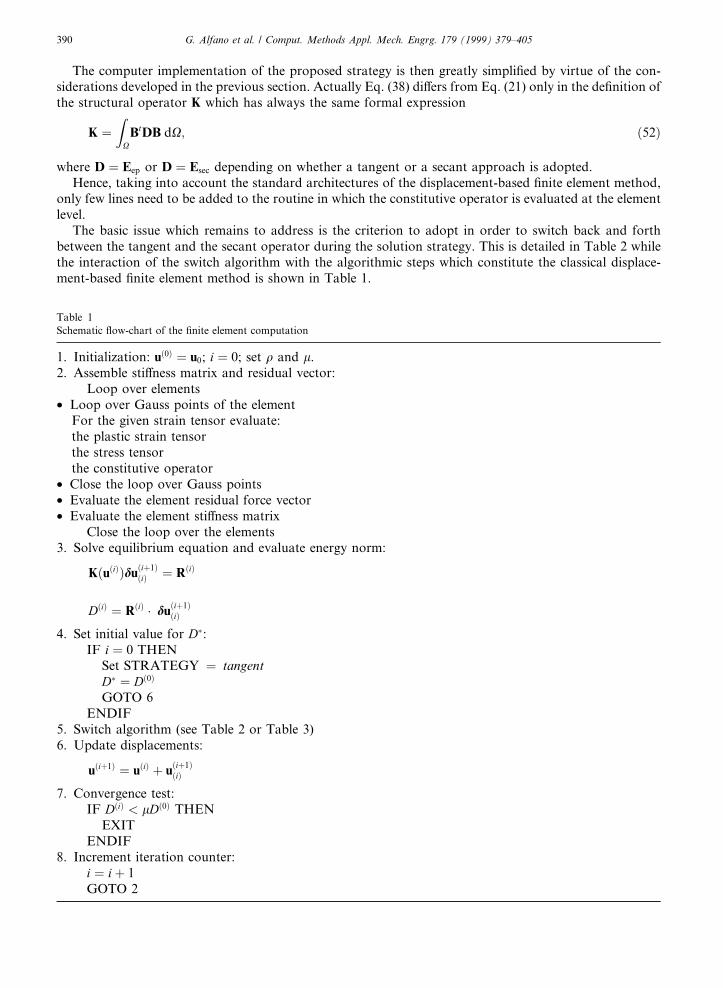
The basic issue which remains to address is the criterion to adopt in order to switch back and forthbetween the tangent and the secant operator during the solution strategy. This is detailed in Table 2 whilethe interaction of the switch algorithm with the algorithmic steps which constitute the classical displace-ment-based ®nite element method is shown in Table 1.

Table 1

Schematic ¯ow-chart of the ®nite element computation

1. Initialization: u�0� � u0; i � 0; set q and l.2. Assemble sti�ness matrix and residual vector:

Loop over elements· Loop over Gauss points of the element

For the given strain tensor evaluate:the plastic strain tensorthe stress tensorthe constitutive operator

· Close the loop over Gauss points· Evaluate the element residual force vector· Evaluate the element sti�ness matrix

Close the loop over the elements3. Solve equilibrium equation and evaluate energy norm:

K�u�i��du�i�1��i� � R�i�

D�i� � R�i� � du�i�1��i�

4. Set initial value for D�:IF i � 0 THEN

Set STRATEGY � tangentD� � D�0�

GOTO 6ENDIF

5. Switch algorithm (see Table 2 or Table 3)6. Update displacements:

u�i�1� � u�i� � u�i�1��i�

7. Convergence test:IF D�i� < lD�0� THEN

EXITENDIF

8. Increment iteration counter:i � i� 1GOTO 2

390 G. Alfano et al. / Comput. Methods Appl. Mech. Engrg. 179 (1999) 379±405

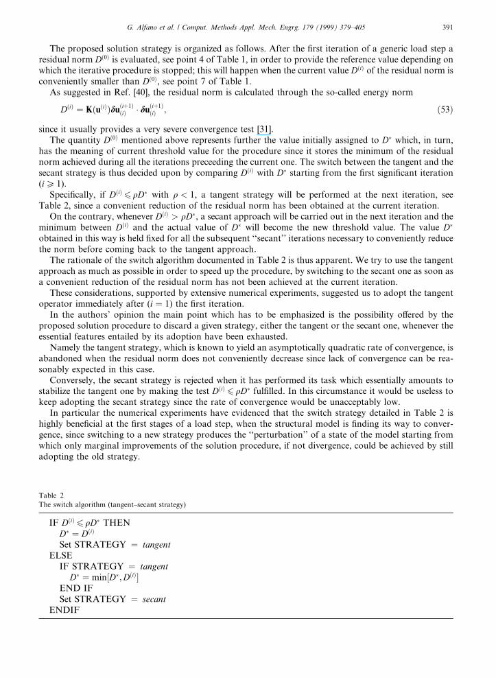
The proposed solution strategy is organized as follows. After the ®rst iteration of a generic load step aresidual norm D�0� is evaluated, see point 4 of Table 1, in order to provide the reference value depending onwhich the iterative procedure is stopped; this will happen when the current value D�i� of the residual norm isconveniently smaller than D�0�, see point 7 of Table 1.

As suggested in Ref. [40], the residual norm is calculated through the so-called energy norm

D�i� � K�u�i��du�i�1��i� � du

�i�1��i� ; �53�

since it usually provides a very severe convergence test [31].The quantity D�0� mentioned above represents further the value initially assigned to D� which, in turn,

has the meaning of current threshold value for the procedure since it stores the minimum of the residualnorm achieved during all the iterations preceeding the current one. The switch between the tangent and thesecant strategy is thus decided upon by comparing D�i� with D� starting from the ®rst signi®cant iteration(i P 1).

Speci®cally, if D�i�6 qD� with q < 1, a tangent strategy will be performed at the next iteration, seeTable 2, since a convenient reduction of the residual norm has been obtained at the current iteration.

On the contrary, whenever D�i� > qD�, a secant approach will be carried out in the next iteration and theminimum between D�i� and the actual value of D� will become the new threshold value. The value D�

obtained in this way is held ®xed for all the subsequent ``secant'' iterations necessary to conveniently reducethe norm before coming back to the tangent approach.

The rationale of the switch algorithm documented in Table 2 is thus apparent. We try to use the tangentapproach as much as possible in order to speed up the procedure, by switching to the secant one as soon asa convenient reduction of the residual norm has not been achieved at the current iteration.

These considerations, supported by extensive numerical experiments, suggested us to adopt the tangentoperator immediately after (i � 1) the ®rst iteration.

In the authors' opinion the main point which has to be emphasized is the possibility o�ered by theproposed solution procedure to discard a given strategy, either the tangent or the secant one, whenever theessential features entailed by its adoption have been exhausted.

Namely the tangent strategy, which is known to yield an asymptotically quadratic rate of convergence, isabandoned when the residual norm does not conveniently decrease since lack of convergence can be rea-sonably expected in this case.

Conversely, the secant strategy is rejected when it has performed its task which essentially amounts tostabilize the tangent one by making the test D�i�6 qD� ful®lled. In this circumstance it would be useless tokeep adopting the secant strategy since the rate of convergence would be unacceptably low.

In particular the numerical experiments have evidenced that the switch strategy detailed in Table 2 ishighly bene®cial at the ®rst stages of a load step, when the structural model is ®nding its way to conver-gence, since switching to a new strategy produces the ``perturbation'' of a state of the model starting fromwhich only marginal improvements of the solution procedure, if not divergence, could be achieved by stilladopting the old strategy.

Table 2

The switch algorithm (tangent±secant strategy)

IF D�i�6 qD� THEND� � D�i�

Set STRATEGY � tangentELSE

IF STRATEGY � tangentD� � min�D�;D�i��

END IFSet STRATEGY � secant

ENDIF

G. Alfano et al. / Comput. Methods Appl. Mech. Engrg. 179 (1999) 379±405 391

Only when the bowl of convergence has been reached the tangent strategy becomes successful to attainboth convergence and a quadratic rate.

We specify that by ``perturbation'' of the structural model we mean the change in the direction of du�i�1��i�

entailed by the tangent or the secant strategy.

4.1. Algorithmic details of the tangent±secant strategy

Let us now turn to discuss some algorithmic details of the tangent±secant strategy and to illustrate somealternative implementations with respect to the one presented in Table 2.

First of all, a sensitivity analysis has been performed on the quantity q of Table 2 in order to establishwhich could be the best value to adopt in numerical calculations.

Recalling that q is always less than 1, we found that values ranging from 0.4 to 0.5 provide the bestcompromise between the necessity of ensuring convergence of the solution procedure and the goal ofkeeping the convergence rate as high as possible.

More speci®cally, greater values of q yield a more frequent adoption of the tangent strategy which caninvalidate convergence although, in our experience, this never happened even with the value q� 0.9. On thecontrary, low values of q are associated with too a high number of secant iterations which appreciablydeteriorate the convergence rate.

It is worth noting that values of q greater than one have been used in Ref. [5], where the tangent±secantstrategy has been successfully applied to no-tension materials by suitably modifying the switch algorithm ofTable 2. Besides the value of q, the essential modi®cations concerned the way in which the threshold valueD� was updated during the iterations.

These last considerations refer to a more general problem which is represented by the possibility ofconsidering a variety of switch algorithms. We detail in particular one of them to provide additional in-sights in the proposed procedure and to discuss some points which will be useful in Section 5 where theenhanced version of the tangent±secant strategy is presented.

It has been previously remarked that small load steps are required to ensure convergence in a puretangent approach unless additional techniques, such as line search, are employed. Our aim is to produce ane�ective, robust solution algorithm which can be comparable, in terms of convergence and numerical ef-®ciency, with a tangent approach combined with line searches.

Let us then consider an FE structural model subject to a load step for which a pure tangent approach,i.e. without line searches, would diverge. What typically happens is that, after the ®rst iteration, the residualnorm decreases and then, in one of the subsequent iterations, increases progressively up to make the so-lution procedure diverge.

There are then two consecutive iterations (iÿ 1 and i) in which the residual norm increases; without lossin generality, we can suppose that D�iÿ1� � D�. In our procedure the tangent strategy, which is the oneadopted immediately after the ®rst iteration, is stopped and the secant operator enters the evaluation of thestructural operator to be employed at the �i� 1�th iteration.

Now the main point is: which displacements one has to consider to evaluate the secant operator? Theones just found or the displacements evaluated at the �iÿ 1�th iteration which are characterized by a valueof the residual norm lower with respect to the current one? Clearly, in this last case, the ith iteration be-comes completely ine�ective.

In the strategy documented in Table 2 we always consider the current values of the displacements but, atleast in principle, it could seem more reasonable to address the displacements associated with D� which, forthe case just examined, are the ones calculated at the �iÿ 1�th iteration.

We also implemented this alternative strategy by evaluating the secant operator with the values of thedisplacements associated with D�, on the additional condition that this value had been determined during a``tangent'' iteration. In the absence of this last condition, the following inconvenience would be originated.

Refer to a sequence of secant iterations after which the condition D�i�6 qD� is ful®lled and D�i� becomesthe new threshold value D�. Assume further that in the following tangent iteration the residual norm in-creases so that a switch to the alternative strategy is made.

We then have to perform a new sequence of secant iterations. However, if we evaluated the secantoperator with the displacements associated with the threshold value D�, ®xed in the last secant iteration, we

392 G. Alfano et al. / Comput. Methods Appl. Mech. Engrg. 179 (1999) 379±405

would ultimately perform two consecutive sets of secant iterations, thus considerably slowing the solutionprocedure.

Numerical experiments obtained with the switch algorithm just described did not yield signi®cant im-provements with respect to the one reported in Table 2. For this reason this alternative strategy wasabandoned, taking also into account the fact that it required an increased computational burden.

5. The enhanced tangent±secant strategy

The tangent±secant strategy illustrated in the previous section allowed us to signi®cantly improve theoverall performances of a pure tangent approach. To ®x the ideas let us make reference to the classicalbenchmark problem of an in®nitely long rectangular strip in plane strain documented in Refs. [31,40].

The eight load steps which are typically necessary to ensure convergence in a pure tangent approach canbe completely avoided in our strategy since the total load, represented by imposed displacements, can beassigned in one step by reducing at the same time the total number of iterations.

Similar performances can be obtained with the tangent approach only by supplementing it with a line-search technique. With speci®c reference to the example cited above this was explicitly stated by Simo andTaylor at page 116 of their paper [31].

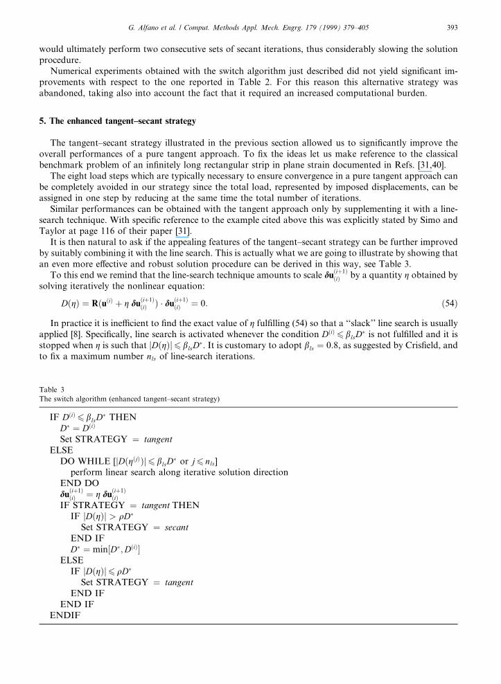
It is then natural to ask if the appealing features of the tangent±secant strategy can be further improvedby suitably combining it with the line search. This is actually what we are going to illustrate by showing thatan even more e�ective and robust solution procedure can be derived in this way, see Table 3.

To this end we remind that the line-search technique amounts to scale du�i�1��i� by a quantity g obtained by

solving iteratively the nonlinear equation:

D�g� � R�u�i� � g du�i�1��i� � � du

�i�1��i� � 0: �54�

In practice it is ine�cient to ®nd the exact value of g ful®lling (54) so that a ``slack'' line search is usuallyapplied [8]. Speci®cally, line search is activated whenever the condition D�i�6blsD

� is not ful®lled and it isstopped when g is such that jD�g�j6 blsD

�. It is customary to adopt bls � 0:8, as suggested by Cris®eld, andto ®x a maximum number nls of line-search iterations.

Table 3

The switch algorithm (enhanced tangent±secant strategy)

IF D�i�6 blsD� THEN

D� � D�i�

Set STRATEGY � tangentELSE

DO WHILE [jD�g�j��j6 blsD� or j6 nls]

perform linear search along iterative solution directionEND DOdu�i�1��i� � g du

�i�1��i�

IF STRATEGY � tangent THENIF jD�g�j > qD�

Set STRATEGY � secantEND IFD� � min�D�;D�i��

ELSEIF jD�g�j6 qD�

Set STRATEGY � tangentEND IF

END IFENDIF

G. Alfano et al. / Comput. Methods Appl. Mech. Engrg. 179 (1999) 379±405 393

Clearly, di�erent implementations of the line-search technique are possible. We shall make reference inparticular to the one contained in the FEAP program [39] which was used in our numerical experiments, seeSection 6.

The ®rst problem we had to face in order to combine the tangent± secant strategy with line searches wasto decide where to insert the line searches iterations: only after each tangent iteration, only after a speci®cnumber, say one or two, of secant iterations or after both of them?

The best strategy turned out to be the last one in the sense that we allowed line searches to be activatedafter each tangent and after each secant iteration even if, in this last case, the need of search iterations wasquite rare.

The second problem we addressed was concerned with the convenience of modifying the value of nls withrespect to the one adopted in the classical implementation. This need was motivated by the followingconsiderations.

Let us make reference to two consecutive ``tangent'' iterations characterized by an increase of the re-sidual norm, a situation which usually produces divergence of the solution procedure if a further tangentiteration is performed without an intermediate line search.

Particularly at the early iterations of a load step, the increase of the residual norm can be of severalorders of magnitude. In this case the line search is almost ine�ective since the value of g tends to zero and itis usually determined by the condition that nls has been reached, see e.g. Tables 4b and 5b.

In practice this means that a lot of computing time has been wasted to ®nd out that the direction du�i�1��i� is

completely wrong, since g! 0, so that the subsequent tangent iteration will be performed from values ofthe displacements almost equal to u�i�.

On the other hand, there is no way to circumvent this drawback of the tangent strategy supplementedby line searches unless an alternative strategy is used to modify the direction du

�i�1��i� determined in a

tangent iteration whenever it fails to be a descent direction for the residual norm. Since we now dispose ofthe secant strategy, the maximum number nls of line-search iterations, assumed to be 10 in FEAP, washalved.

A further choice we had to make was to decide the strategy to adopt at the end of line search iterations.In other words did we have to switch to the alternative strategy (from tangent to secant or vice versa)anyway or could it be more appropriate to keep performing iterations with the previous strategy? Further,on the basis of which parameter we had to decide in one sense or in the other one?

It was soon clear that the value jD�g�j evaluated at the end of the line search, rather than g itself, had toplay the most prominent role. We thus decided to perform a tangent (secant) iteration whether jD�g�j was(was not) conveniently smaller than the threshold value D� evaluated at the previous iterations.

In other words it seemed natural to consider a su�ciently low value of jD�g�j as a reasonable expectationthat a subsequent tangent iteration could have been successful.

However, D�g� is de®ned by Eq. (54) and hence it does not strictly have the meaning of a residualnorm, as given by Eq. (53). For this reason we made tighter the condition on D�g�, with respect to theone which stops line searches, by setting jD�g�j6 qD� since q is always less than bls. Depending onwhether the test is satis®ed or not a tangent or a secant approach will be adopted at the next iteration,see Table 3.

As a ®nal remark, it is worth noting that line search de®nitely alleviates the intrinsic drawbacks of boththe tangent and secant strategies. Actually, on one hand it increases the stability properties of the tangentapproach, and on the other side, it is able of accelerating the secant strategy by reducing the relevantnumber of iterations required in the solution strategy.

In our experience the number of line searches along a ``secant'' direction was very small, two as amaximum, and they turned out to be necessary only at the ®rst iterations of a load step, since these aretypically the most critical ones for convergence.

6. Numerical examples

We present two well-known examples selected from the literature that illustrate the performances ofthe solution strategies detailed in the previous sections. The examples were run on a 233 MHz Pentium

394 G. Alfano et al. / Comput. Methods Appl. Mech. Engrg. 179 (1999) 379±405

based machine by using the program FEAP, version 6.4 b [39], developed by Profs. R.L. Taylor andJ.C. Simo. The results have been obtained by adopting the values q � 0:5, bls � 0:8 and l � 10ÿ16, seeTable 1.

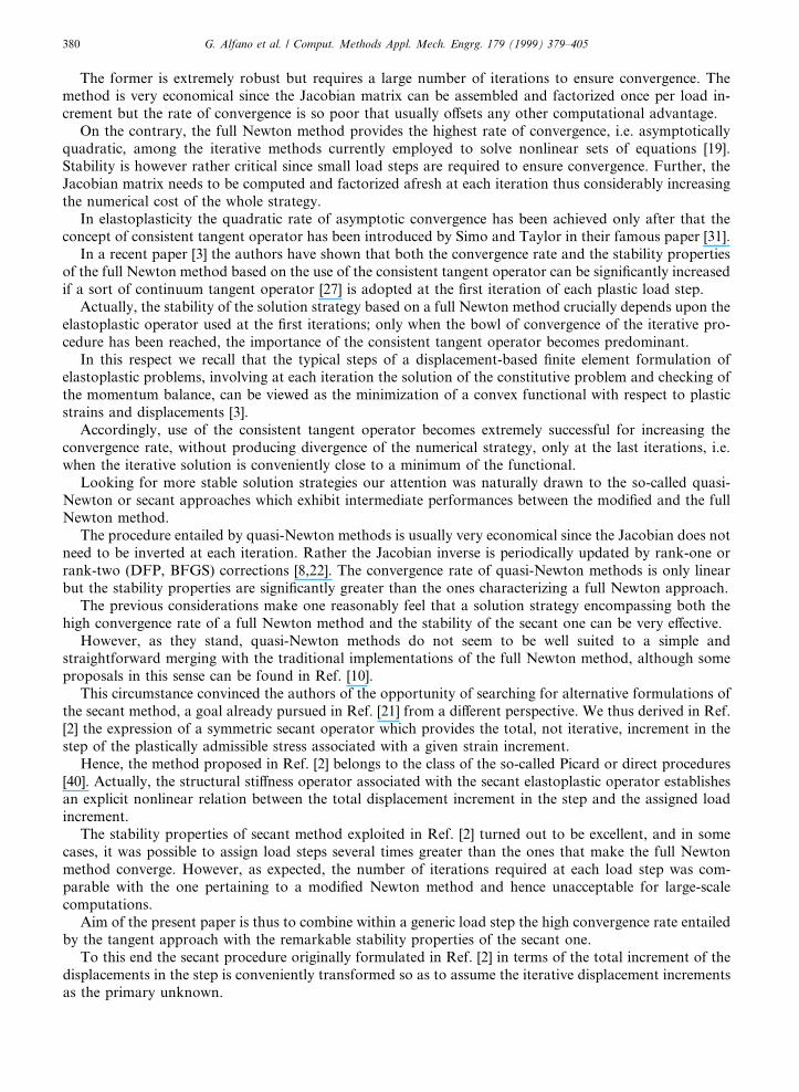
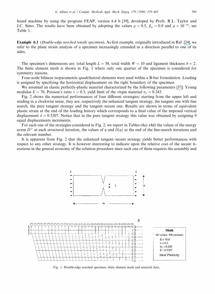
Example 6.1 (Double-edge notched tensile specimen). As ®rst example, originally introduced in Ref. [24], werefer to the plane strain analysis of a specimen increasingly extended in a direction parallel to one of itssides.

The specimen's dimensions are: total length L � 30, total width W � 10 and ligament thickness b � 2.The ®nite element mesh is shown in Fig. 1 where only one quarter of the specimen is considered forsymmetry reasons.

Four-node bilinear isoparametric quadrilateral elements were used within a B-bar formulation. Loadingis assigned by specifying the horizontal displacement on the right boundary of the specimen.

We assumed an elastic perfectly-plastic material characterized by the following parameters [37]: Youngmodulus E � 70, Poisson's ratio m � 0:3, yield limit of the virgin material ry � 0:243.

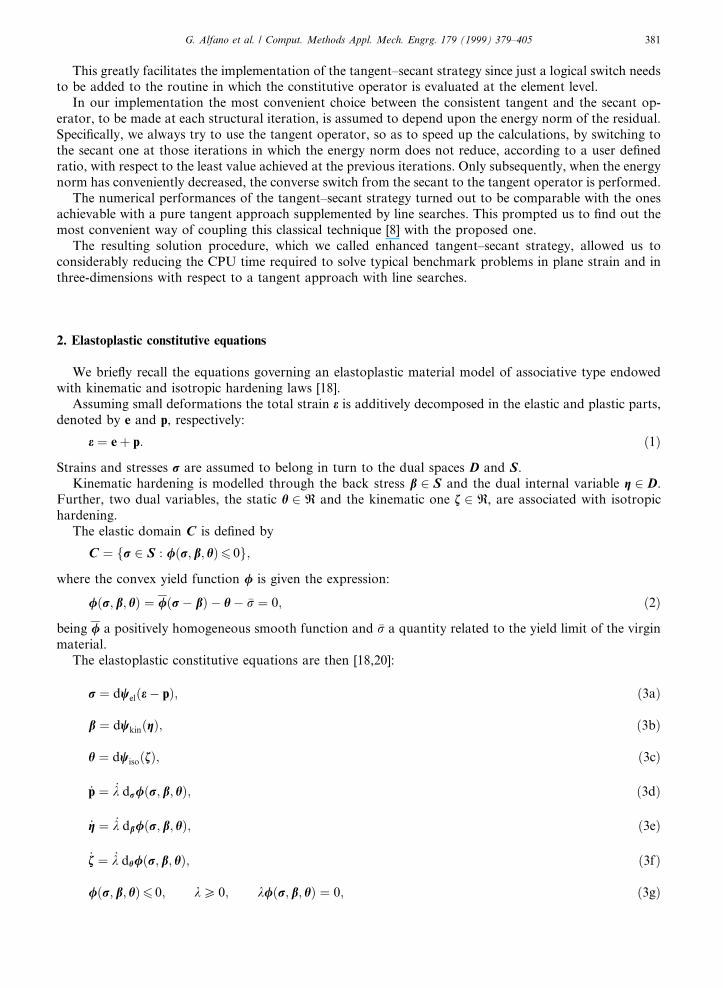
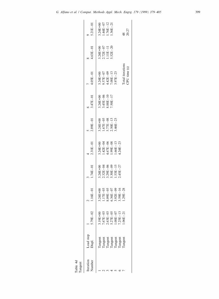
Fig. 2 shows the numerical performances of four di�erent strategies; starting from the upper left andreading in a clockwise sense, they are, respectively the enhanced tangent strategy, the tangent one with linesearch, the pure tangent strategy and the tangent±secant one. Results are shown in terms of equivalentplastic strain at the end of the loading history which corresponds to a ®nal value of the imposed verticaldisplacement d � 0:5207. Notice that in the pure tangent strategy this value was obtained by assigning 9equal displacements increments.

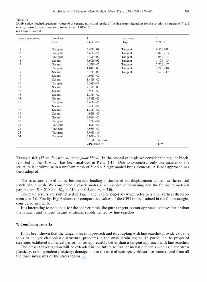
For each one of the strategies considered in Fig. 2, we report in Tables (4a)±(4d) the values of the energynorm D�i� at each structural iteration, the values of g and D�g� at the end of the line-search iterations andthe relevant number.

It is apparent from Fig. 2 that the enhanced tangent±secant strategy yields better performances withrespect to any other strategy. It is however interesting to indicate upon the relative cost of the secant it-erations in the general economy of the solution procedure since each one of them requires the assembly and

Fig. 1. Double-edge notched specimen: ®nite element mesh and material data.

G. Alfano et al. / Comput. Methods Appl. Mech. Engrg. 179 (1999) 379±405 395

the factorization of the structural operator, a burden not required by line search which operates at theelement level.

For this reason more re®ned meshes were considered and CPU times for the four strategies of Fig. 2 havebeen plotted in Fig. 3 versus the number of mesh elements. The results documented in Fig. 3 make onereasonably assess that the numerical performances reported in Fig. 2 are substantially una�ected by thedimension of the mesh.

Fig. 2. Double-edge notched specimen: compared overall performances and plot of the equivalent plastic strain.

396 G. Alfano et al. / Comput. Methods Appl. Mech. Engrg. 179 (1999) 379±405

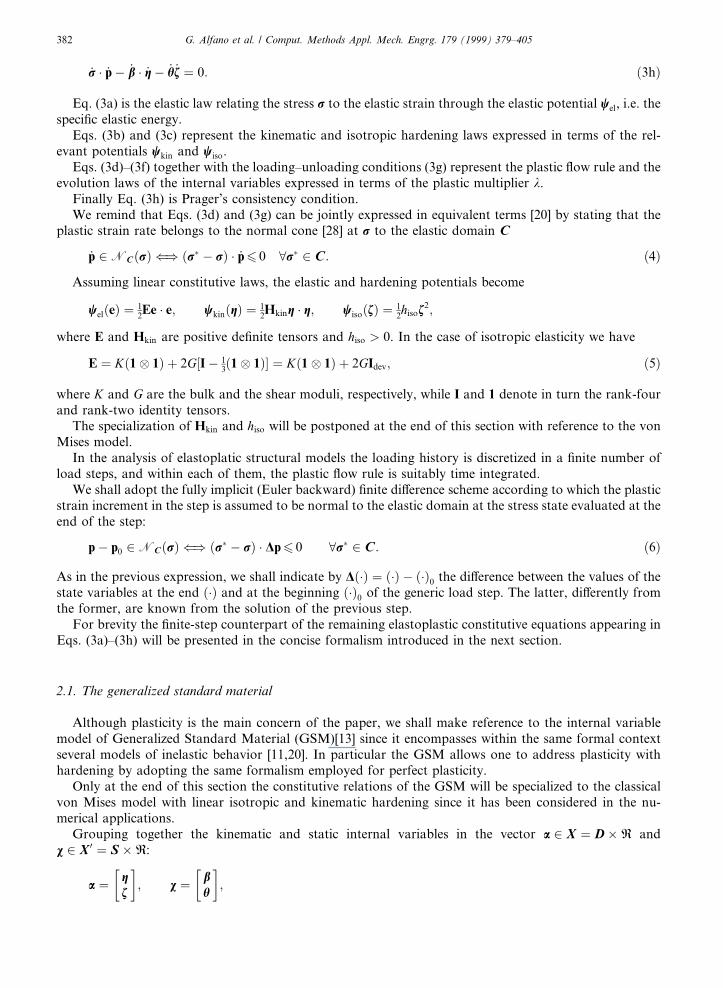
Example 6.2 (Three-dimensional rectangular block). In the second example we consider the regular block,reported in Fig. 4, which has been analyzed in Refs. [1,15]. Due to symmetry, only one-quarter of thestructure is idealized with a uniform mesh of 5� 5� 5 eight-noded brick elements. A B-bar approach hasbeen adopted.

The structure is ®xed at the bottom and loading is simulated via displacement control at the centralpatch of the mesh. We considered a plastic material with isotropic hardening and the following materialparameters: E � 210:000, Hiso � 210, m � 0:3 and ry � 250.

The main results are synthetized in Fig. 5 and Tables (5a)±(5d) which refer to a ®nal vertical displace-ment d � 2:0. Finally, Fig. 6 shows the comparative values of the CPU times attained in the four strategiesconsidered in Fig. 5.

It is interesting to note that, for the coarser mesh, the pure tangent±secant approach behaves better thanthe tangent and tangent±secant strategies supplemented by line searches.

7. Concluding remarks

It has been shown that the tangent±secant approach and its coupling with line searches provide valuabletools to analyze elastoplastic structural problems in the small strain regime. In particular the proposedstrategies exhibited numerical performances appreciably better than a tangent approach with line searches.

The present investigation will be extended in the future to further inelastic models such as plane stressplasticity, rate-dependent plasticity, damage and to the case of isotropic yield surfaces constructed from allthe three invariants of the stress tensor [23].

Table 4a

Double-edge notched specimen: values of the energy norm and results of the line-search iterations for the solution strategies of Fig. 2

(energy norm for each time step; tolerance l� 1.0Eÿ16)

(a) Tangent±secant

Iteration number Load step 1 Load step 2

Displ. 2.60Eÿ01 Displ. 5.21Eÿ01

1 Tangent 6.45E+01 Tangent 6.57E+01

2 Tangent 5.40Eÿ01 Tangent 1.02Eÿ03

3 Tangent 3.49E+02 Tangent 3.08Eÿ04

4 Secant 3.60E+02 Tangent 1.19Eÿ05

5 Secant 4.55Eÿ02 Tangent 2.70Eÿ07

6 Tangent 1.04E+00 Tangent 3.74Eÿ10

7 Secant 3.15E+00 Tangent 3.52Eÿ17

8 Secant 4.03Eÿ02

9 Secant 1.49Eÿ02

10 Tangent 7.38Eÿ01

11 Secant 2.19E+00

12 Secant 3.92Eÿ02

13 Secant 1.37Eÿ02

14 Secant 6.84Eÿ03

15 Tangent 7.45Eÿ02

16 Secant 2.42Eÿ01

17 Secant 1.32Eÿ02

18 Secant 4.92Eÿ03

19 Secant 2.09Eÿ03

20 Tangent 8.26Eÿ04

21 Tangent 3.87Eÿ04

22 Tangent 6.95Eÿ07

23 Tangent 3.04Eÿ10

24 Tangent 3.03Eÿ16

Total iterations 31

CPU time (s) 14.39

G. Alfano et al. / Comput. Methods Appl. Mech. Engrg. 179 (1999) 379±405 397

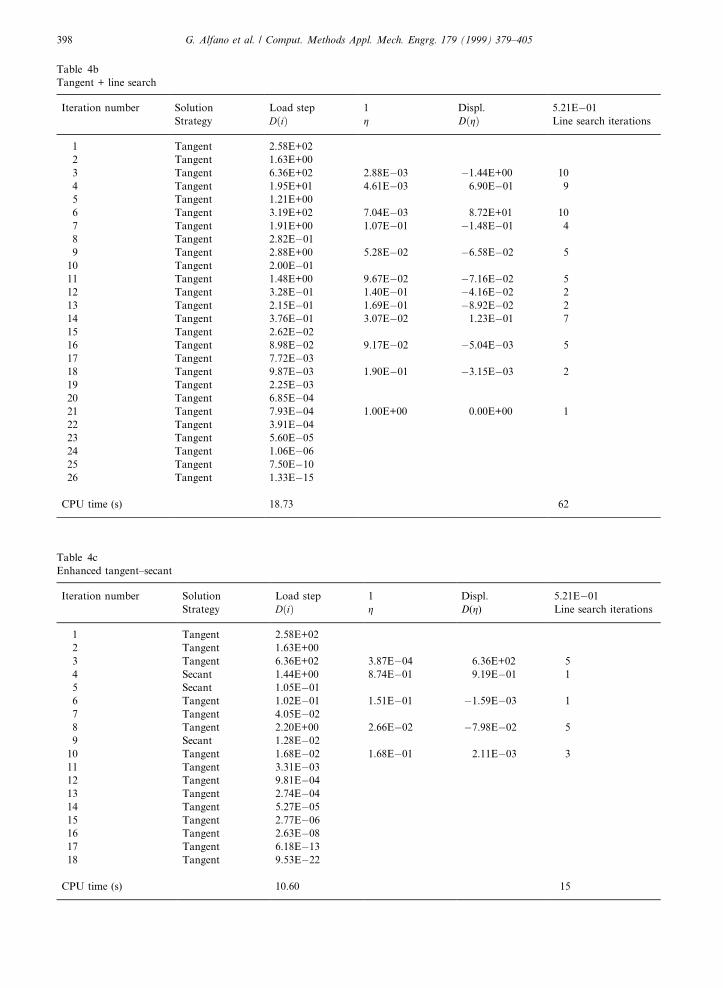
Table 4b

Tangent + line search

Iteration number Solution Load step 1 Displ. 5.21Eÿ01

Strategy D�i� g D�g� Line search iterations

1 Tangent 2.58E+02

2 Tangent 1.63E+00

3 Tangent 6.36E+02 2.88Eÿ03 ÿ1.44E+00 10

4 Tangent 1.95E+01 4.61Eÿ03 6.90Eÿ01 9

5 Tangent 1.21E+00

6 Tangent 3.19E+02 7.04Eÿ03 8.72E+01 10

7 Tangent 1.91E+00 1.07Eÿ01 ÿ1.48Eÿ01 4

8 Tangent 2.82Eÿ01

9 Tangent 2.88E+00 5.28Eÿ02 ÿ6.58Eÿ02 5

10 Tangent 2.00Eÿ01

11 Tangent 1.48E+00 9.67Eÿ02 ÿ7.16Eÿ02 5

12 Tangent 3.28Eÿ01 1.40Eÿ01 ÿ4.16Eÿ02 2

13 Tangent 2.15Eÿ01 1.69Eÿ01 ÿ8.92Eÿ02 2

14 Tangent 3.76Eÿ01 3.07Eÿ02 1.23Eÿ01 7

15 Tangent 2.62Eÿ02

16 Tangent 8.98Eÿ02 9.17Eÿ02 ÿ5.04Eÿ03 5

17 Tangent 7.72Eÿ03

18 Tangent 9.87Eÿ03 1.90Eÿ01 ÿ3.15Eÿ03 2

19 Tangent 2.25Eÿ03

20 Tangent 6.85Eÿ04

21 Tangent 7.93Eÿ04 1.00E+00 0.00E+00 1

22 Tangent 3.91Eÿ04

23 Tangent 5.60Eÿ05

24 Tangent 1.06Eÿ06

25 Tangent 7.50Eÿ10

26 Tangent 1.33Eÿ15

CPU time (s) 18.73 62

Table 4c

Enhanced tangent±secant

Iteration number Solution Load step 1 Displ. 5.21Eÿ01

Strategy D�i� g D(g) Line search iterations

1 Tangent 2.58E+02

2 Tangent 1.63E+00

3 Tangent 6.36E+02 3.87Eÿ04 6.36E+02 5

4 Secant 1.44E+00 8.74Eÿ01 9.19Eÿ01 1

5 Secant 1.05Eÿ01

6 Tangent 1.02Eÿ01 1.51Eÿ01 ÿ1.59Eÿ03 1

7 Tangent 4.05Eÿ02

8 Tangent 2.20E+00 2.66Eÿ02 ÿ7.98Eÿ02 5

9 Secant 1.28Eÿ02

10 Tangent 1.68Eÿ02 1.68Eÿ01 2.11Eÿ03 3

11 Tangent 3.31Eÿ03

12 Tangent 9.81Eÿ04

13 Tangent 2.74Eÿ04

14 Tangent 5.27Eÿ05

15 Tangent 2.77Eÿ06

16 Tangent 2.63Eÿ08

17 Tangent 6.18Eÿ13

18 Tangent 9.53Eÿ22

CPU time (s) 10.60 15

398 G. Alfano et al. / Comput. Methods Appl. Mech. Engrg. 179 (1999) 379±405

Tab

le4

d

Tan

gen

t

Iter

ati

on

Lo

ad

step

12

34

56

78

9

Nu

mb

erD

isp

l.5

.79

Eÿ0

21

.16

Eÿ0

11.7

4Eÿ0

12.3

1Eÿ0

12.8

9Eÿ0

13.4

7Eÿ0

14.0

5Eÿ0

14.6

3Eÿ0

15.2

1Eÿ0

1

1T

an

gen

t3

.19

E+

00

3.2

4E

+00

3.2

4E

+00

3.2

4E

+00

3.2

4E

+00

3.2

4E

+00

3.2

4E

+00

3.2

4E

+00

3.2

4E

+00

2T

an

gen

t7

.67

Eÿ0

31

.17

Eÿ0

32.3

2Eÿ0

41.4

2Eÿ0

41.6

7Eÿ0

53.4

5Eÿ0

69.5

7Eÿ0

72.7

2Eÿ0

71.4

4Eÿ0

7

3T

an

gen

t2

.63

Eÿ0

38

.09

Eÿ0

53.2

9Eÿ0

64.6

7Eÿ0

65.7

7Eÿ0

88.8

8Eÿ1

04.4

2Eÿ0

91.1

1Eÿ1

11.7

6Eÿ1

2

4T

an

gen

t5

.27

Eÿ0

56

.36

Eÿ0

75.3

0Eÿ0

91.9

9Eÿ0

82.5

0Eÿ1

37.5

0Eÿ1

77.0

8Eÿ1

35.5

2Eÿ2

01.3

6Eÿ2

1

5T

an

gen

t1

.08

Eÿ0

73

.92

Eÿ0

91.5

3Eÿ1

51.6

6Eÿ1

33.4

6Eÿ2

33.9

7Eÿ2

3

6T

an

gen

t7

.25

Eÿ1

33

.59

Eÿ1

62.4

5Eÿ2

74.2

4Eÿ2

3

7T

an

gen

t1

.06

Eÿ2

11

.29

Eÿ2

8T

ota

lit

erati

on

s48

CP

Uti

me

(s)

20.2

7

G. Alfano et al. / Comput. Methods Appl. Mech. Engrg. 179 (1999) 379±405 399

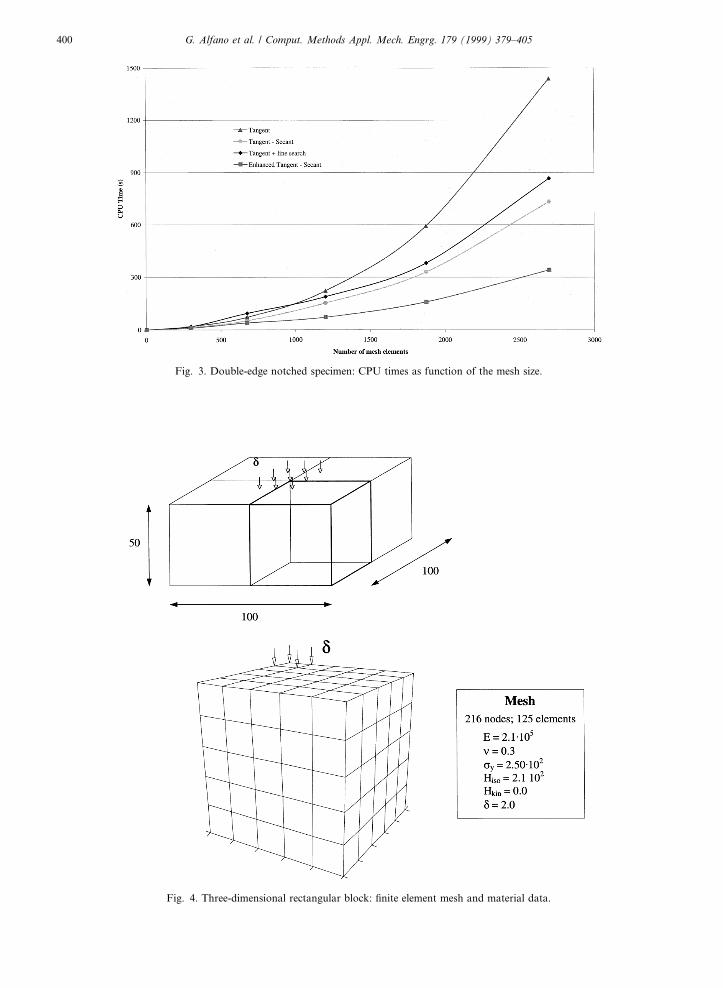
Fig. 3. Double-edge notched specimen: CPU times as function of the mesh size.

Fig. 4. Three-dimensional rectangular block: ®nite element mesh and material data.

400 G. Alfano et al. / Comput. Methods Appl. Mech. Engrg. 179 (1999) 379±405

Additional numerical experiments will concern the opportunity of modifying the value of q during thestructural iterations, see Tables 2 and 3, as function, e.g., of the ratio between D�i� and D�0�.

Table 5a

Three-dimensional rectangular block: values of the energy norm and results of the line-search iterations for the solution strategies of

Fig. 5

(a) Tangent±secant

Iteration number Load step 1

Displ. 2.00E+00

1 Tangent 1.40E+07

2 Tangent 2.11E+06

3 Tangent 2.16E+07

4 Secant 3.65E+07

5 Secant 1.93E+05

6 Tangent 2.85E+06

7 Secant 5.70E+06

8 Secant 6.55E+04

9 Tangent 9.61E+04

10 Secant 1.72E+05

11 Secant 8.06E+03

12 Tangent 1.18E+03

13 Tangent 1.54E+02

14 Tangent 3.34E+00

15 Tangent 3.48Eÿ03

16 Tangent 1.46Eÿ05

17 Tangent 9.06Eÿ14

CPU time (s) 14.44

Table 5b

Tangent + line search

Iteration number Solution Load step 1 Displ. 2.00E+00

Strategy D�i� g D (g) Line search iterations

1 Tangent 1.40E+07

2 Tangent 2.11E+06

3 Tangent 2.16E+07 4.82Eÿ02 ÿ9.87E+04 9

4 Tangent 1.98E+05

5 Tangent 2.90E+05 4.60Eÿ01 ÿ1.04E+05 1

6 Tangent 3.13E+05 2.02Eÿ01 ÿ1.48E+05 3

7 Tangent 7.20E+04

8 Tangent 1.04E+06 8.17Eÿ02 ÿ4.91E+04 6

9 Tangent 8.24E+04 1.80Eÿ01 ÿ3.47E+04 2

10 Tangent 2.20E+04

11 Tangent 5.95E+05 4.47Eÿ02 ÿ3.89E+02 10

12 Tangent 7.91E+03

13 Tangent 3.75E+03

14 Tangent 1.95E+04 2.55Eÿ01 ÿ8.15E+02 4

15 Tangent 5.14E+02

16 Tangent 1.18E+01

17 Tangent 4.27Eÿ01

18 Tangent 8.91Eÿ05

19 Tangent 6.37Eÿ12

CPU time (s) 22.74 35

G. Alfano et al. / Comput. Methods Appl. Mech. Engrg. 179 (1999) 379±405 401

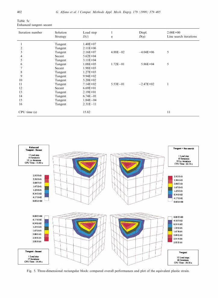
Fig. 5. Three-dimensional rectangular block: compared overall performances and plot of the equivalent plastic strain.

Table 5c

Enhanced tangent±secant

Iteration number Solution Load step 1 Displ. 2.00E+00

Strategy D�i� g D(g) Line search iterations

1 Tangent 1.40E+07

2 Tangent 2.11E+06

3 Tangent 2.16E+07 4.88Eÿ02 ÿ4.04E+06 5

4 Secant 5.62E+04

5 Tangent 3.11E+04

6 Tangent 1.08E+05 1.72Eÿ01 5.86E+04 5

7 Secant 1.98E+03

8 Tangent 1.27E+03

9 Tangent 9.94E+02

10 Tangent 5.20E+02

11 Tangent 7.14E+02 5.53Eÿ01 ÿ2.47E+02 1

12 Secant 6.69E+01

13 Tangent 2.19E+01

14 Tangent 6.74Eÿ01

15 Tangent 1.84Eÿ04

16 Tangent 2.31Eÿ11

CPU time (s) 15.82 11

402 G. Alfano et al. / Comput. Methods Appl. Mech. Engrg. 179 (1999) 379±405

Tab

le5

d

Tan

gen

t

Iter

ati

on

Lo

ad

step

12

34

56

78

910

11

12

13

Nu

mb

erD

isp

l.1

.54

Eÿ0

13

.08

Eÿ0

14

.62

Eÿ0

16.1

5Eÿ0

17.6

9Eÿ0

19.2

3Eÿ0

11.0

8E

+00

1.2

3E

+00

1.3

8E

+00

1.5

4E

+00

1.6

9E

+00

1.8

5E

+00

2.0

0E

+00

1T

an

gen

t8

.29

E+

04

7.8

8E

+0

48

.37

E+

04

8.4

8E

+04

8.5

1E

+04

8.5

3E

+04

8.5

4E

+04

8.5

4E

+04

8.5

4E

+04

8.5

3E

+04

8.5

2E

+04

8.5

0E

+04

8.4

9E

+04

2T

an

gen

t1

.32

E+

04

1.7

4E

+0

21

.56

E+

01

1.9

7E

+00

1.3

2E

+00

4.1

0Eÿ0

12.4

0Eÿ0

11.3

6Eÿ0

13.5

9Eÿ0

11.2

7Eÿ0

11.1

5Eÿ0

11.1

0Eÿ0

11.0

5Eÿ0

1

3T

an

gen

t5

.64

E+

03

8.9

0Eÿ0

12

.22

Eÿ0

23.9

3Eÿ0

52.8

4Eÿ0

53.4

9Eÿ0

61.9

5Eÿ0

61.3

4Eÿ0

67.9

3Eÿ0

61.1

3Eÿ0

68.0

0Eÿ0

75.4

1Eÿ0

74.1

6Eÿ0

7

4T

an

gen

t1

.32

E+

03

7.4

2Eÿ0

32

.14

Eÿ0

84.5

4Eÿ1

48.4

5Eÿ1

41.5

4Eÿ1

51.8

8Eÿ1

62.8

5Eÿ1

61.1

1Eÿ1

41.9

2Eÿ1

68.1

9Eÿ1

73.1

1Eÿ1

71.6

1Eÿ1

7

5T

an

gen

t6

.82

E+

02

2.2

6Eÿ0

92

.20

Eÿ1

9

6T

an

gen

t1

.57

E+

02

1.6

9Eÿ2

1

7T

an

gen

t9

.10

Eÿ0

1

8T

an

gen

t5

.70

Eÿ0

6

9T

an

gen

t3

.20

Eÿ1

5T

ota

l

iter

ati

on

s

60

CP

Uti

me

(s)

50.7

0

G. Alfano et al. / Comput. Methods Appl. Mech. Engrg. 179 (1999) 379±405 403

Acknowledgements

The ®nancial support of the C.N.R. (National Research Council) is gratefully acknowledged.

References

[1] U. Andel®nger, E. Ramm, D. Roehl, Two-dimensional and three-dimensional enhanced assumed strain elements and their

applications in plasticity, in: Proceedings of the third International Conference on Comp. Plast., Barcelona, Pineridge, Swansea,

1992.

[2] G. Alfano, L. Rosati, N. Valoroso, A secant-like strategy for ®nite element solutions in elastoplasticity, Proc. of XIII Nat. Conf.

AIMETA 3 (1997) 145±150.

[3] G. Alfano, L. Rosati, N. Valoroso, A displacement-like ®nite element model for J2 elastoplasticity variational formulation and

®nite-step solution, Comput. Meth. Appl. Mech. Engrg. 155 (1998) 325±358.

[4] G. Alfano, L. Rosati, A general approach to the evaluation of consistent tangent operators for rate-independent elastoplasticity,

Comput. Meth. Appl. Mech. Engrg., in press, 1998.

[5] G. Alfano, L. Rosati, N. Valoroso, A numerical strategy for ®nite element analysis of no-tension materials, submitted to Int. J.

Numer. Meth. Engrg., 1998.

[6] G. Alfano, L. Rosati, N. Valoroso, Closed-form evaluation of the consistent tangent operator for isotropic yield criteria of

arbitrary type, in: Proceedings of WCCM IV, Buenos Aires, 1998.

[7] F. Auricchio, R.L. Taylor, J. Lubliner, Application of a return map algorithm to plasticity models, in: D.R.J. Owen et al. (Eds.),

Computational Plasticity, Proceedings of the 3rd International Conference, Pineridge, Swansea, 1992, pp. 2229±2248.

[8] M.A. Cris®eld, Nonlinear Finite Element Analysis of Solids and Structures 1, Wiley, England, 1991.

[9] P. Fuschi, D. Peric, D.R.J. Owen, Studies in generalized midpoint integration in rate-independent plasticity with reference to plane

stress J2-¯ow theory, Comput. and struct. 43 (1992) 1117±1133.

[10] M. Geradin, S. Idelsohn, M. Hogge, Compuational strategies for the solution of large nonlinear problems via quasi-Newton

methods, Comput. and Struct. 13 (1981) 73±81.

[11] P. Germain, Q.S. Nguyen, P. Suquet, Continuum thermodynamics, J. Appl. Mech. ASME 50 (1983) 1010±1020.

[12] G.H. Golub, C.F. Van Loan, Matrix computations, The John Hopkins University Press, Baltimore, MD, 1989.

[13] B. Halphen, Q.S. Nguyen, Sur les materiaux standards g�en�eralis�es, J. Mech. 14 (1975) 39±63.

[14] G. Hofstetter, J.C. Simo, R.L. Taylor, A modi®ed cap model: closest point solution algorithms, Comput. and Struct. 46 (1993)

203±214.

[15] E.P. Kasper, R.L. Taylor, A mixed-enhanced strain method: linear problems, University of California at Berkeley, Report no.

UCB/SEMM-97/02, 1997.

[16] R.D. Krieg, S.W. Key, Implementation of a time dependent plasticity theory into structural computer programs, Constitutive

Equations in Viscoplasticity: Computational and Engeneering Aspects, AMD-20, ASME, New York, 1976.

Fig. 6. Three-dimensional rectangular block: CPU times as function of the mesh size.

404 G. Alfano et al. / Comput. Methods Appl. Mech. Engrg. 179 (1999) 379±405

[17] R.D. Krieg, D.B. Krieg, Accuracies of numerical solutions methods for elastic-perfectly plastic model, J. Pressure Vessel Tech.

A.S.M.E. 99 (1977) 510±515.

[18] J. Lubliner, Plasticity Theory, Macmillan, New York, 1990.

[19] D.G. Luenberger, Linear and Nonlinear Programming, 2nd ed., Addison-Wesley, Reading, 1984.

[20] F. Marotti de Sciarra, L. Rosati, A uni®ed formulation of elastoplastic models by an internal variable approach, in: D.R.J. Owen

et al. (Eds.), Computational Plasticity, Proceedings of the fourth International Conference, Pineridge, Swansea, 1995, pp. 153±164.

[21] J.B. Martin, W.W. Bird, A secant approach for holonomic elastoplastic incremental analysis with a von Mises yield function, Eng.

Comput. 3 (1986) 192±201.

[22] H. Matthies, G. Strang, The solution of nonlinear ®nite element equations, Int. J. Numer. Meth. Engrg. 14 (1979) 1613±1626.

[23] H. Matzenmiller, R.L. Taylor, A return mapping algorithm for isotropic elastoplasticity, Int. J. Numer. Meth. Engrg. 37 (1994)

813±826.

[24] J.C. Nagtegaal, J.C. Parks, J.C. Rice, On numerically accurate ®nite element solutions in the fully plastic range, Comput. Meth.

Appl. Mech. Engrg. 4 (1974) 153±177.

[25] M. Ortiz, E.P. Popov, Accuracy and stability of integration algorithms for elastoplastic constitutive relations, Int. J. Numer.

Meth. Engrg. 21 (1985) 1561±1576.

[26] M. Ortiz, J.C. Simo, An analysis of a new class of integration algorithms for elastoplastic constitutive relations, Int. J. Numer.

Meth. Engrg. 23 (1986) 353±366.

[27] D.R.J. Owen, E. Hinton, Finite Elements in Plasticity: Theory and Practice, Pineridge, Swansea, 1980.

[28] R.T. Rockafellar, Convex Analysis, Princeton University Press, Princeton, 1970.

[29] G. Romano, L. Rosati, F. Marotti, de Sciarra, A critical review of extremal paths and work functionals in elastoplasticity, Int. J.

Eng. An. Des. 2 (1995) 83±95.

[30] H.L. Schreyer, R.F. Kulak, M.M. Kramer, Accurate numerical solutions for elastic±plastic models, J. Pressure Vessel Tech.

ASME. 101 (1979) 226±234.

[31] J.C. Simo, R.L. Taylor, Consistent tangent operators for rate-independent elastoplasticity, Comput. Meth. Appl. Mech. Engrg. 48

(1985) 101±118.

[32] J.C. Simo, M. Ortiz, A uni®ed approach to ®nite deformation elastoplasticity, Comput. Meth. Appl. Mech. Engrg. 49 (1986) 221±

245.

[33] J.C. Simo, R.L. Taylor, A return mapping algorithm for plane stress elastoplasticity, Int. J. Numer. Meth. Engrg. 22 (1986) 649±

670.

[34] J.C Simo, J.W. Ju, Strain and stress based continuum damage models ± Part II: computational aspects, Int. J. Solids and

Structures 23 (7) (1987) 841±869.

[35] J.C. Simo, S. Govindjee, Nonlinear B-stability and symmetry preserving return mapping algorithms for plasticity and

viscoplasticity, Int. J. Numer. Meth. Engrg. 31 (1991) 151±176.

[36] J.C. Simo, Algorithms for static and dynamic multiplicative plasticity that preserve the classical return mapping schemes of the

in®nitesimal theory, Comput. Meth. Appl. Mech. Eng. 99 (1992) 61±112.

[37] S.L. Weissman, M. Jamian, Two-dimensional elastoplasticity: approximation by mixed ®nite elements, Int. J. Numer. Meth.

Engrg. 36 (1993) 3703±3727.

[38] M.L. Wilkins, Calculation of elastic±plastic ¯ow, in: (Ed.), Methods of Computational Physics 3, Academic Press, New York,

1964.

[39] R.L. Taylor, FEAP User Manual, vers. 6.4, University of California at Berkeley, 1998.

[40] O.C. Zienkiewicz, R.L. Taylor, The Finite Element Method, 4th ed., vols. 1 and 2, McGraw Hill, New York, 1991.

G. Alfano et al. / Comput. Methods Appl. Mech. Engrg. 179 (1999) 379±405 405