Computational Techniques
22
Computational Techniques Prof. Dr. Niket Kaisare Department of Chemical Engineering Indian Institute of Technology, Madras Module No. # 08 Lecture No. # 02 Ordinary Differential Equations (Boundary Value Problem) (Refer Slide Time: 00:27) Hello, and welcome to lecture 2 of module 8 and this particular lecture we are going to use Microsoft excel, in order to solve an example of ODE boundary value problem using the shooting method. What we have been doing in this particular module is to saw look at methods to solve ODE, boundary value problems and this specific example that we are going to take - this is the example that we discussed in the previous module - is heat conduction in a rod. This rod is, let us say the length of the rod is 2 meters, one end of the rod is kept at 30 degrees Celsius, the other end is kept at 80 degrees Celsius and this rod loses heat to the atmosphere the atmosphere is also at 30 degrees Celsius. And the overall equation that we can obtain from this particular system is d square T by dx squared equal to beta multiplied by T minus 30, where the value of beta is going to be equal to 0.01.
-
Upload
khangminh22 -
Category
Documents
-
view
1 -
download
0
Transcript of Computational Techniques

Computational Techniques Prof. Dr. Niket Kaisare
Department of Chemical Engineering Indian Institute of Technology, Madras
Module No. # 08
Lecture No. # 02
Ordinary Differential Equations (Boundary Value Problem)
(Refer Slide Time: 00:27)
Hello, and welcome to lecture 2 of module 8 and this particular lecture we are going to use Microsoft excel, in order to solve an example of ODE boundary value problem using the shooting method. What we have been doing in this particular module is to saw look at methods to solve ODE, boundary value problems and this specific example that we are going to take - this is the example that we discussed in the previous module - is heat conduction in a rod. This rod is, let us say the length of the rod is 2 meters, one end of the rod is kept at 30 degrees Celsius, the other end is kept at 80 degrees Celsius and this rod loses heat to the atmosphere the atmosphere is also at 30 degrees Celsius.
And the overall equation that we can obtain from this particular system is d square T by dx squared equal to beta multiplied by T minus 30, where the value of beta is going to be equal to 0.01.

So, this is the example that we are going to take in this particular module. In order to solve this by using a shooting method we are going to convert this boundary value problem of course, subject to 2 boundary conditions that is T 0 equal to 30 and T 2 equal to 80. This is the problem that we have, we are going to convert into a first order ODEs and in order to do that we are going to write our y equal to T and z equal to T dash.
So, our first equation is going to be dy by dx is going to be nothing but z. So, our first equation is dy by dx equal to z, our second equation is d by dx of dT by dx and dT by dx is nothing but z. So, dz by dx is going to be equal to beta multiplied by T minus 30, T is nothing but y. So, beta multiplied by y minus 30. And our boundary value,or the original boundary value is y 0 is going to be equal to 30 and the other boundary value is y 2 equal to 80.
So, this is our original problem. The way we are going to convert this into an initial value problem is, we are going to guess z 0 and modify these guesses such that finally we reach y 2 equal to 80 and we are going to modify using bisection method. So, this is going to be our strategy for ODE, boundary value problem using the shooting method.
So, to recap the boundary value problem that we are interested in solving is these two equations subject to these two boundary conditions. Instead of that we are going to solve the same initial value problem with condition y 0 equal to 30 and we will keep wearing the condition z 0 such that finally, we should be able to match the condition y 2 equal to 80. So that is the problem that we are going to look at using Microsoft excel.

(Refer Slide Time: 05:22)
So, what I have done over here is I have written down that is it I will just have got ready. So, now we will solve this ODE boundary value problem using Microsoft excel. Again, when I use the term Microsoft excel I do not necessarily mean you have to use Microsoft excel in order to solve a problem. Any kind of a spreadsheet such as the open office or the Google spreadsheet is going to be good enough in order to solve any of the problems that we are doing in this particular module or for that matter this entire course.
So, what I have written over here is the original boundary value problem. We have T double dash equal to beta multiplied by T minus 30, the value of beta we have chosen as 0.01, so I will write that down over here, and T 0 equal to 30 and T 2 equal to 80. What we have done just now on the board is we have converted this into an initial value problem by substituting T equal to y and T dash equal to z.
So, our first equation is going to be dy by dx that is y dash is going to be equal to z that is our first equation. Our second equation is dz by dx, which is nothing but T double dash. So, dz by dx is going to be equal to 0.01 multiplied by T minus 30, T in this case is y, so y minus 30.
So, these are our 2 equations in 2 unknowns y and z; we require 2 initial conditions. The first initial condition is given by one of the boundary conditions and that is y 0 equal to 30, the second initial condition we will use z 0 equal to guess and these guesses will be made such that finally, we are interested in satisfying the boundary value y 2 equal to 80. So that is the value, that we

are interested in satisfying. So, we will make these guesses such that we end up shooting accurately at y 2 equal to 80.
So, this is our entire problem statement. So, what we are going to do is, we are going to use the midpoint method for solving the ODE problem; solve ODE-IVP using midpoint method. We have done this midpoint method in our previous module, I am going to recap this overall midpoint method. This time we are going do this midpoint method for a two dimensional problem; we have a problem in two variables. I will just zoom on to the full screen mode, so that we can view the entire thing more easily. We will start off with, so what we need to define is we need to define our h, h we are going to define. Let say for this particular problem we will define h as say 0.01, again I will quickly go through the choice of h also in this particular example.
So, we will start off with x equal to 0 and we will have y and our z over here, y 0 we are going to start off at 30, as I had said earlier. z 0 we will start off as 0, keep in mind z equal to 0 basically means that the gradient at the entry is going to be equal to 0. What that essentially should lead us to that irrespective of whether what we are going, what numerical procedure we are going to follow, our temperatures throughout the entire reactor should remain steady at 30 degrees because there is no heat transfer that is going to take place under these conditions.
So, let see whether our method is able to get that or not. And now, we require for midpoint method we will require k 1 for variable 1, and we will require k 1 for variable 2 k 1. For variable 1 is going to be nothing but y equal to z value that comes over here. So, this is going to be our k 1; k 1 for variable 2 is going to be nothing but 0.01 multiplied by y minus 30.
So, k 1 is obtained through this particular equation, our k 1 for the second variable is obtained through these equations. So, k 1 for the first variable is nothing but k 1 equal to z computed at the location i, and k 2 is nothing but 0.01 multiplied by y i minus 30. In order to compute k 2 using the midpoint method, we need to obtain y. So, in order at the midpoint method what we need is, we require to compute f of x plus h by 2 and y plus h k 1 by 2. So, this is the function value that we need to compute.
So, basically we need the value of y plus h multiplied by k 1 by 2, likewise we need the value of z also. This is going to be y i or I will just drop the subscripts and superscripts over here, h multiplied by k 1 by 2 and this is what we have function and just do format cells, so that looks better and do the format cells for here also.
So, this is going to be y plus h k 1 by 2 and likewise we will have z plus h k 1 by 2. So, this is what we need for the computation of this function value. So, this is going to be equal to y plus h

multiplied by k 1 1 by 2 and we will put the dollar signs, this is what we have been doing all throughout the h value does not change. So, instead of having B 8 we are going to have dollar B, dollar 8.
So that is going to be y plus h k 1 1 by 2, and we also need z plus h k 1 2 by 2. So, z plus h multiplied by k 1 2 by 2 and we can do again as before, we will put dollar signs over here, and then we will basically need k 2 1 and we will need k 2 2. And k 2 1 and k 2 2 are just going to be computed in the same manner as before; so I will just copy and paste and we will just do f 2 and we will see k 2 1 is going to be from this particular equation. So, y dash equal to z, so k 2 is going to be z computed at the midpoint. The midpoint is given by x plus h by 2 comma z plus h k 1 by 2. So, this is the value of k 2 1 and likewise the value of k 2 2 is going to be equal to 0.01 multiplied by this guy minus 30 that is going to be the value of k 2 1.
Our next x is going to be x plus h and again as always we will put dollars in front of this h; so that is going to be our next x. Our y is going to be nothing but y plus h multiplied by k 2, so that is our midpoint method. In our midpoint method, we have y i plus 1 equal to y i plus h multiplied by k 2 and that is what we will have over here, it should be writing instead of h, I should be putting this particular guy.
(Refer Slide Time: 15:55)
And I will put dollars over there so that whenever we are going to just drag and drop we are not that value is not going to change and likewise, z is i plus 1 is going to be z i plus h multiplied by

k 2 and for h again I will put the dollar signs. And this particular row I will just copy it to the next row and we will take this entire row and we will copy the entire row below 2 meters.
If instead of 0.01 if we had 0.02, if we had h equal to anything else our results are not going to change, because the overall ambient is at 30 degrees, the initial condition is at 30 degrees. So, if there is no gradient initial into to the system, the overall system is going to remain at 30.
So, the results that we are going to get are the results that we have obtain from the midpoint method do match our intuition. So, I will write this as midpoint boundary value problem with bisection.
(Refer Slide Time: 17:02)
So, now we are going to use the bisection method in order to solve this boundary value problem. So, what do I mean by that is, what I am going to do over here is list out the various values that we are going to get. So, our y 2 target is 80 and what I am going to write over here is, y 2 calculated is going to be equal to the y 2 value that we get is the y value at length of 2. So that is going to be our y 2 calculated and we are going to solve this entire thing using the bisection method. So, just resize this a little bit, so that we can observe everything that happens.
So, in this section now, this is the ODE IVP using the midpoint method and I will have this as the bisection method. Now, the bisection is what we are going to use in order to solve for shooting to our final solution.

So, this is going to be our z 0 guess and this is going to be our y 2 minus 80 and I have resized this little bit more. So, our initial z 0 guess was equal to 0 with that z 0 guess equal to 0. The y 2 minus 80 this is what I will write over here, y 2 minus 80 is going to be equal to y 2 calculated minus 80, so this is what we will get. So, y 2 minus 80 is going to minus 50, I will copy this and paste the value over here, paste special values and the value is pasted over there.
So, let us see what guess z 0 equal to 100 gives us. So, what I am going to do is the guess over here is going to be changed to 100 and with the guess equal to 100 the value y 2, calculated value turns out to be 151 degrees. So, I will copy this and I will paste this over here.
So, what we have is with z 0 guess equal to 0; we have our temperature as 30 degrees or deviation from 80 degrees boundary was minus 50. The deviation from 80 degrees boundary using an initial guess of 100 was 151.
So, now, we are going to shoot at the midpoint between the 2. So that shoot is going to be equal to into be equal to the previous guy plus the next guy by 2; so that is the new short is going to be 50. So, what we are going to do is, we are going to take this value, z 0 value, this is our z 0 value and I will color all these guys also that it is easier for us to realize what is happening over here.
(Refer Slide Time: 21:57)
So, with z 0 equal to 0 our deviation was minus 50, with z 0 equal to 100 our deviation was 150. So, we are going to change our z 0 to 50 and see what we get. With the change of z 0 to 50 the temperature is 130, whereas the deviation from our temperature is 50. So, I will copy that and paste it over here and again I am only going to paste values, right click and paste special values

only and so our next point has to be a midpoint between 0 and 50; so that midpoint is going to be equal to 25.
(Refer Slide Time: 22:39)
(Refer Slide Time: 23:02)
So, we are going to change that initial guess to 25, with that guess change to 25 our temperature that we are shooting at becomes 80.334; we can copy this and paste it over here, paste special values. Now, again our value is going to lie between 0 and 25 that midpoint is. So, it is going to be equal to 25 divided by 2 which is 12.5; so we replace this by 12.5.

So, when we change this to 12.5 what we are getting is that the temperature at the end of 2 meters ends up being 55. So that is what happens over here what I will also do is, I will just plot the temperature and I will do insert and scatter plot as we use to do before we will do a temperature versus the location plot over here.
(Refer Slide Time: 23:44)
So, now, let us go to full screen mode and see what is happening. So that we are able to see this in a more, we will get a clearer picture about this. So, when we took our initial guess as 100 what we want to do, we will also insert a line; so this thin line is our target that is the target we intend to reach and we go to full screen mode.
So, initially when we had our z 0 equal to 0 our temperature remained flat, that is, the thick line is the temperature profile it remained flat and we were shooting much below the intended value of 80 when we change this value to 100, we shot to the intended instead of in intended value of 80, we hit at 1 at 230.
So, then we decreased this from 100 to 50 and with 50 we are hitting at the intended value. Instead of 18 as the intended value, we were hitting that at 130 was the temperature at the other end.
(Refer Slide Time: 25:15)
So, next we tried 25 through the bisection rule and we are now very close to 80, again the error is 0.33. If this error is acceptable to us, we stop our iteration; if this is not acceptable to us, then we are going to change this again.
(Refer Slide Time: 25:33)
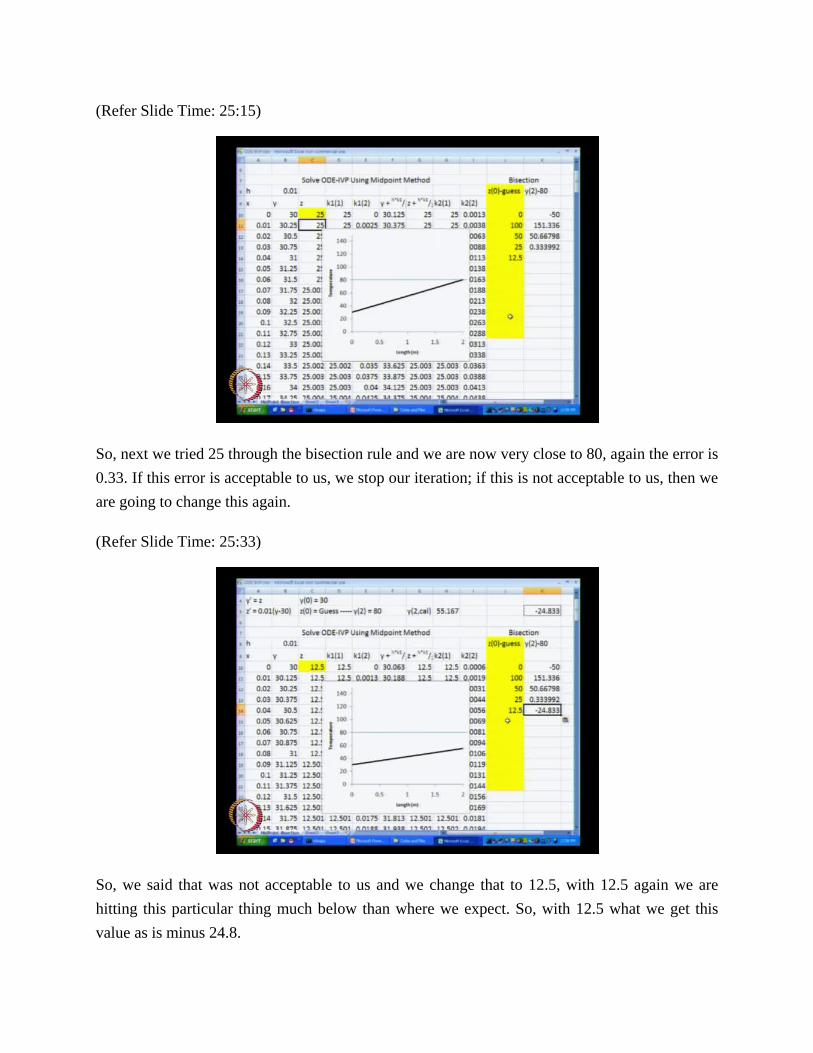
So, we said that was not acceptable to us and we change that to 12.5, with 12.5 again we are hitting this particular thing much below than where we expect. So, with 12.5 what we get this value as is minus 24.8.

(Refer Slide Time: 25:57)
So, the next value is going to be between 12.5 and 25, because they lie on either side of the guess and so the next value that we are going to try is 18.5 for z 0 and with 18.5, we are getting this as minus 12. Keep in mind that, again we are shooting below the desired point. So, now, what we have done is the next value that we got is 18.575 as the next value. From the bisection method when we substitute 18.75 and then solve the ODE IVP using the midpoint method this is the temperature curve that we are going to get.
So, the next guess of at the temperature that we are reaching is less than 80 which is signified by the negative value, again that we get of y 2 minus 80, which basically means we are going to replace 12.5 as the guess, and so the 2 guesses that we are going to have is 18.75 and 25 and we are going to take an average of the 2.

(Refer Slide Time: 27:12)
So, we will take 25 plus 18.75 divided by 2 that is going to be our next guess of z 0; we copy that and paste the value over there using paste special values. And now, we have gotten again closer to the solution from when the guess was 18.75 the value over here is, minus 5.95, again this value is negative.
(Refer Slide Time: 27:45)
So, we are going to replace 18.75 as the guess, with 21.875 as the guess and we are going to take the average between the 2 values 21.875 plus 25 divided by 2. We are going to continue this, I

forgot to tell you that we need to predefine what our stopping criterion is going to be. And in this particular example let us use a stopping criterion that y 2 minus 80 should be less than 0.1. So, we are fairly close with the initial guess as 25, let us try to get even closure to that solution, this particular value has to fall below 0.1, the absolute value should fall below 0.1.
So, 23.4375 we copy that and paste it as our z 0 using paste special, as we have been doing so far and again as you see that this temperature has in closure to the actual 80 degree Celsius value. We copy this and paste it over here, again using paste special and because this is a negative value, we are going to retain the solution 25 and replace the other solution with 23.43.
(Refer Slide Time: 28:56)

(Refer Slide Time: 29:22)
(Refer Slide Time: 29:46)
So, we will take the average of 23.43 and 25, which lie on either side of the solution and thus this becomes our new average; we copy it and we paste it in the yellow block over here using paste special and now the value that we reach is minus 1.24 that is the value that we have reached over here. Now, again because this value is negative, we take an average between 24.2 and 25 that would be our next guess and we will use this particular value and substituted as z 0 using paste special as before and now we have reached minus 0.45 again this is negative value. So, again we take an average between 24.6 and 25 as our next guess hopefully which we should converge.

Now, again we have copied this and pasted it in the yellow block over here, which signifies z 0, paste special values and yes.
So, finally, we have converged paste special values. So, finally we have converged to our solution; we will get the solution when our z 0 guess is approximately 24.8 and when the value of z 0 is 24.8. We have reached the temperature exit at the temperature at the end of the rod as 80 degrees Celsius and this is how the temperature changes; it changes linearly between 30 degrees Celsius and 80 degree Celsius between within the rod.
So, the problem that we had was one end of the rod was kept at 30, the other end of the rod was kept at 80 and there was heat loss taking place to the surroundings from this particular system and this is the overall result that we are going to get from this particular reactor.
And this is how we have ended up approaching the overall solution. We took a guess value of z 0 based on the guess value of z 0 solved initial value problem and obtained the value that we will get at the end of the rod and then we use that particular information in order to guess a new value of z 0 and with that over and over again and finally we reached the desired value that we were interested in.
So that is essentially how we have gone about solving this particular problem. Now, let us just recap what we have done; we will go back to our board and we will try to recap the overall procedure that we have followed in this particular example.
(Refer Slide Time: 32:08)

So, let us recap what we have really done in solving the ODE boundary value problem using the shooting method. The problem that we had was of the form d square T by dx square equal to, I am just going to put that as some function of T dT by dx and x. I am just going to write this as a general function in in this particular form. And the boundary conditions that over give into us were, T 0 equal to some value alpha and T L equal to some value beta, instead of T L give into us we could have been given T dash L equal to beta. So, let us say if we had two different cases, we had or T L equal to beta or T dash of L equal to beta, this is also another possibility for the boundary condition.
So, now we had to solve these problems. This was the original problem; we converted this through change of variables, where variable y was defined equal to T, variable z was defined as equal to T dash. As a result of this, the equations that we got, the first equation was dy by dx was equal to z; the second equation was d by dx of dT by dx which makes it dz by dx. So, dz by dx was equal to function f of y z and x, y, z ; x and this were subject to the boundary conditions y 0 equal to alpha and the other boundary condition was either y L equal to beta or z L equal to beta one of the 2 conditions.
(Refer Slide Time: 34:46)
So, for example if the other end is insulated we will have z L equal to beta or if the other end is the temperature is specified as it was in this particular problem, we would have y L equal to beta. So, this is the overall problem and instead of solving it for y 0 equal to alpha and y L equal to beta, instead of that we solve an initial value problem. Aand the initial value problem that we solved was dy by dx equal to z dz by dx equal to f of y z and x, subject to y 0 equal to alpha and

z 0 not y and z 0 equal to some value phi, let us say this as phi and when we solve this particular problem this will give us y and z as a function of x.
So, for example the temperature changes like this and the overall dT by dz probably changes somewhat like this. So, this is how z goes and this is how y goes, and this is the value at y L. And let say we had the problem of solving, y L should be equal to beta, then we define our function capital f of phi as equal to y L minus beta.
So, this is our capital F, where y L obtained by solving ODE initial value problem. So, what we did in our non-linear equations part of the course, which was module 4 is, this particular function F of phi was a function that was explicitly given to us. For example, the example that we took was 2 minus 2 plus x minus l n x. In that particular case, the function was explicitly given to us, we knew that this is the overall function and based on that we could find out whether certain value satisfy f of x equal to 0 or not in this particular case we have not been given explicit function in the variable phi, but we have implicitly defined this function in variable phi by solving this ODE initial value problem every time, we change phi our value y at the end of the rod changes.
(Refer Slide Time: 37:52)
So, for one particular value of phi, for value of phi 1 we will get this as our y L. For certain value of phi 2, we will get this as our y L so on and so forth. So, by solving this overall ODE initial value problem, as we change our initial value phi from phi to phi 1, phi 1 to phi 2, phi 2 to phi 3 so on and so forth. We are getting different values at the end of the rod. using Now, using this

different values of the end of the rod, we want to ensure that they come as close as possible to the value beta.
So, this is the problem that we are going to solve. So, what we did was we the first value we took was, we took phi equal to 0 in the example that we solved using Microsoft excel. When we use phi equal to 0, we got F of phi as minus 80. Next, we use our phi equal to 100 that was the second guess that we took, phi equal to 100 basically meant that the initial slope we gave was a very large slope.
When we gave an initial slope as the very large slope, the temperature at the end of the rod ended being something like 230, because the temperature was 230; 230 minus 80 we got that as a value 150. Because these two values where on either side of the true solution the true solution that we wanted is, F of phi equal to 0. Because they lied on the either side we could use basically the bisection method in order to change the value from phi equal to 0 to from phi equal to 0 and phi equal to 100. We could change it to phi equal to 50 instead of using bisection method at this stage we could have use any other method of our choice. For example, if we had used the Regula Falsi method, we would have gotten phi 3 as nothing but 100 minus this guy minus this guy divided by this minus this value the whole thing multiplied by phi at 100 that was how we get got the Regula Falsi method. So, the way we will get the Regula Falsi method is basically, x i minus x i minus x i minus 1 divided by f i minus f i minus 1 whole thing multiplied by f i.
So, this is what we can do so this is this guy and the overall thing we can have that as 150 minus minus 80 divided by not 150 minus minus 80 that is going to be in the denominator has this as 100 minus 0 divided by 150 minus minus 80 so that is plus 80 multiplied by 150.
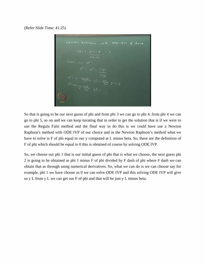
(Refer Slide Time: 41:25)
So that is going to be our next guess of phi and from phi 3 we can go to phi 4, from phi 4 we can go to phi 5, so on and we can keep iterating that in order to get the solution that is if we were to use the Regula Falsi method and the final way to do this is we could have use a Newton Raphson's method with ODE IVP of our choice and in the Newton Raphson’s method what we have to solve is F of phi equal to our y computed at L minus beta. So, these are the definition of F of phi which should be equal to 0 this is obtained of course by solving ODE IVP.
So, we choose our phi 1 that is our initial guess of phi that is what we choose, the next guess phi 2 is going to be obtained as phi 1 minus F of phi divided by F dash of phi where F dash we can obtain that as through using numerical derivatives. So, what we can do is we can choose say for example, phi 1 we have choose as 0 we can solve ODE IVP and this solving ODE IVP will give us y L from y L we can get our F of phi and that will be just y L minus beta.

(Refer Slide Time: 43:47)
Next, we can solve ODE IVP for phi 1 plus delta phi let say we choose our delta phi as 0.01. So, we solve this overall ODE IVP for this particular value solve IVP which will give us the value of y L which was obtained for phi equal to 0.01 from this we will get F of phi plus delta phi which is again the same as y obtain at the end of the rod minus minus beta.
So, now, this particular value let us call this value is nothing but F of phi plus delta phi this value is nothing but F of phi we can use these two guys and our F dash of phi is going to be approximately equal to F of phi plus delta phi minus F of phi divided by delta phi.
So, which we can write that as equal to y of L computed with z 0 equal to phi plus delta phi minus y of L computed using z 0 equal to phi the whole thing divided by delta phi. So, we can use this particular expression for F dash and then with this expression our phi 2 or in general our phi i plus 1 is going to be equal to phi i plus not plus minus F divided by F dash and F dash is going to be obtained in this particular form.
So, we can write this as minus y of L computed at z 0 equal to phi multiplied by delta phi this whole thing should be divided by y L at phi plus delta phi minus y l at phi we choose and initial guess for the initial value z 0 that is going to be phi 1 using phi 1 and a choice of delta phi a delta phi. We can take it as relatively small value and this particular case for example I have taken delta phi as 0.01.
So, we choosing small enough delta phi, we can calculate our y so that is, in this particular case that is the temperature at the end of the rod with the initial value being equal to 0.01. We have
already computed the temperature at the end of the rod with an initial value equal to 0 the difference between the 2 divided by with the delta phi will give us F dash. F dash f divided by F dash is going to give us the amount by which we have to move our phi i.
So, this is going to be what we get as the Newton Raphson’s method. So, what we have done essentially is converted ODE boundary value problem into an ODE initial value problem. We choose and initial guess or two initial guesses for which to solve the ODE initial value problem, if we have 2 initial guesses which lie on either sides of the solution we can either use the bisection method as I showed you in excel or we can use Regula Falsi method as I have demonstrated over here.
So, we can use the Regula Falsi method or bisection method to get a new choice. An alternative way to do this instead of using a bisection or Regula Falsi method is to use a Newton Raphson’s method and if we were to use a Newton Raphson’s method, this is what our expression is going to be where keep in mind this y L is the solution through a numerical scheme of solving an ODE initial value problem, instead of having this as a given function f of x.
So, this is the overall procedure for solving a boundary value problem using shooting method.
(Refer Slide Time: 43:47)
Now, while the shooting method in principle is indeed applicable for this system and we have shown in this particular example its applicability. One of the problems with the shooting method is that the ODE initial value problems that we obtain through this procedure or often going to be unstable. We have seen what instability means, when we talked about ODE initial value

problems in the previous module, what we mean by instability is that under certain conditions, we quickly go to our solution, quickly reaches plus infinity or minus infinity for certain choice of phi values.
So, if that is what happens from the overall system, we will not be able to solve the initial value problems, I will take up quick example in the next lecture. So, in the next lecture of this module we will start off with a quick example where this particular thing happens. We will go over that example and we will then go ahead and make a comparison between. You know ODE boundary value problem solution for this particular example of temperature in a rod and compare it with the ODE boundary value problem for the reactor that we are going to use in the next lecture, that we will motivate, that we will use in to show certain problems with the boundary value problem solution using the shooting method and finally we will go on to the solving this problem using a finite difference method. So that going to be an agenda for our next lecture and see you in the next lecture. Thank you.