
Alternative Route Techniques
346
Alternative Route Techniques and their Applications to the Stochastic on-time Arrival Problem zur Erlangung des akademischen Grades eines Doktors der Ingenieurwissenschaften / Doktors der Naturwissenschaften von der Fakultät für Informatik des Karlsruher Instituts für Technologie (KIT) genehmigte Dissertation von Moritz Helge Kobitzsch aus Berlin Tag der mündlichen Prüfung: 06.11.2015 Erster Gutachter: Herr Prof. Dr. Peter Sanders Zweiter Gutachter: Herr Andrew Goldberg, PhD
-
Upload
khangminh22 -
Category
Documents
-
view
0 -
download
0
Transcript of Alternative Route Techniques
Alternative Route Techniquesand their Applications to the Stochastic on-time Arrival Problem
zur Erlangung des akademischen Grades eines
Doktors der Ingenieurwissenschaften /Doktors der Naturwissenschaften
von der Fakultät für Informatikdes Karlsruher Instituts für Technologie (KIT)
genehmigte
Dissertation
von
Moritz Helge Kobitzsch
aus Berlin
Tag der mündlichen Prüfung: 06.11.2015
Erster Gutachter: Herr Prof. Dr. Peter Sanders
Zweiter Gutachter: Herr Andrew Goldberg, PhD

In memory of my sister.
ii

"Piled Higher and Deeper" by Jorge Cham (www.phdcomics.com)
This thesis is based on 80 914 lines of code1. According to SLOCCount, this puts thecoding work alone at an estimated twenty-one years of development. The credibility(s.a.) is backed by 90 358 words, distributed over 7 448 lines of LaTex code.
1Data generated using David A. Wheeler’s ’SLOCCount’
iii


� Acknowledgements
This thesis presents not only my own work. Many of the topics discussed in this workare strongly influenced by many different people, without whom this thesis would havenot been possible. There is no way of putting a clear number on the relevance of theirinput; the order in which they are listed is purely coincidental and should not reflectany meaning.
First, I would like to thank all of my co-authors. I owe Samitha Samaranayake, forintroducing me to the stochastic on-time arrival problem and all the fruitful discussionswe had. Dennis Schieferdecker, your input on the different topics we worked on togetheras well as your support during my own endeavours are greatly appreciated. DennisLuxen I have to thank for his countless contributions to our work on route corridors.Not only for the route corridors, but also for a great experience during my short stayat Microsoft Research, I owe gratitude to Daniel Delling and Renato Werneck whoboth taught me a lot. Thank you for all the help you have given me and your support,not only in my professional but also in my personal life.
In addition, I have to thank all of my coworkers and office mates that made life atthe institute as good as it could be. I specifically am grateful to Sebastian Schlag forall the fruitful discussions over coffee, to Timo Bingmann for his support in systemmaintenance and his efforts in the office social events. I thank Christian Schulzfor supplying his partitioner and trying out adjustments to better support my ownalgorithms and Jochen Speck for his general support in managing our compute servers.
Furthermore, I have to give thanks to my students that helped a great deal inaccomplishing the results presented in my thesis. Both Marcel Radermacher andStephan Erb have engaged me in most interesting discussions and have provided agreat deal of input. Also, Valentin Buchhold helped a great deal by implementing a lotof useful tools and algorithms for me.
Last, but not least, I have to thank my friends and family for all the moral supportover the duration of this work. I especially owe gratitude to my mother for all her
v

support in not only proofreading my publications but also this thesis. Sina Schmittand Vera Döttling, thank you for all your intense moral support during hard times.
vi

� Contents
1 Introduction 11.1 Context . . . . . . . . . . . . . . . . . . . . . . . . . . . . . . . . . . . 2
1.1.1 Algorithm Engineering in Route Planning . . . . . . . . . . . . 21.2 Contribution and Thesis Outline . . . . . . . . . . . . . . . . . . . . . . 3
I An Introduction to Speed-up Techniques and AlternativeRoutes 7
2 Preliminaries 92.1 On Road Network Representations . . . . . . . . . . . . . . . . . . . . 92.2 Data Structures . . . . . . . . . . . . . . . . . . . . . . . . . . . . . . . 11
2.2.1 Graph Representation . . . . . . . . . . . . . . . . . . . . . . . 112.2.2 Priority Queue . . . . . . . . . . . . . . . . . . . . . . . . . . . 122.2.3 Graph Traversal . . . . . . . . . . . . . . . . . . . . . . . . . . . 14
2.3 Shortest Paths . . . . . . . . . . . . . . . . . . . . . . . . . . . . . . . . 152.3.1 Problem Definition . . . . . . . . . . . . . . . . . . . . . . . . . 152.3.2 SSSP Variations . . . . . . . . . . . . . . . . . . . . . . . . . . . 16
2.4 Algorithms . . . . . . . . . . . . . . . . . . . . . . . . . . . . . . . . . . 172.4.1 The Labelling Algorithm . . . . . . . . . . . . . . . . . . . . . . 172.4.2 Dijkstra’s Algorithm . . . . . . . . . . . . . . . . . . . . . . . . 182.4.3 The Bellman-Ford Algorithm . . . . . . . . . . . . . . . . . . . 19
2.5 Further Concepts and Notations . . . . . . . . . . . . . . . . . . . . . . 21
3 Speeding up Dijkstra’s Algorithm 233.1 Goal Direction . . . . . . . . . . . . . . . . . . . . . . . . . . . . . . . . 253.2 Separator-Based Techniques . . . . . . . . . . . . . . . . . . . . . . . . 27
vii

Contents
3.3 Hierarchical Approaches . . . . . . . . . . . . . . . . . . . . . . . . . . 283.4 Additional Techniques . . . . . . . . . . . . . . . . . . . . . . . . . . . 29
4 Shortest Paths Details 334.1 Contraction Hierarchies . . . . . . . . . . . . . . . . . . . . . . . . . . . 33
4.1.1 Construction . . . . . . . . . . . . . . . . . . . . . . . . . . . . 334.1.2 Query Algorithm . . . . . . . . . . . . . . . . . . . . . . . . . . 354.1.3 Batched Shortest Path using Contraction Hierarchies . . . . . . 374.1.4 Dynamic Implementation . . . . . . . . . . . . . . . . . . . . . . 394.1.5 Theoretical Results . . . . . . . . . . . . . . . . . . . . . . . . . 39
4.2 Customizable Route Planning . . . . . . . . . . . . . . . . . . . . . . . 414.2.1 Construction . . . . . . . . . . . . . . . . . . . . . . . . . . . . 414.2.2 Customization . . . . . . . . . . . . . . . . . . . . . . . . . . . . 434.2.3 Query Algorithm . . . . . . . . . . . . . . . . . . . . . . . . . . 444.2.4 Real Time Customization . . . . . . . . . . . . . . . . . . . . . 46
5 Alternative Routes - a Snapshot 495.1 Alternative Graphs . . . . . . . . . . . . . . . . . . . . . . . . . . . . . 54
5.1.1 Computation . . . . . . . . . . . . . . . . . . . . . . . . . . . . 555.1.2 Recent Improvements . . . . . . . . . . . . . . . . . . . . . . . . 58
5.2 The Via-Node Paradigm . . . . . . . . . . . . . . . . . . . . . . . . . . 595.2.1 The Concept of Viability . . . . . . . . . . . . . . . . . . . . . . 595.2.2 Current Implementations . . . . . . . . . . . . . . . . . . . . . . 625.2.3 Relaxation . . . . . . . . . . . . . . . . . . . . . . . . . . . . . . 64
6 Experimental Methodology 676.1 Hardware and Environment . . . . . . . . . . . . . . . . . . . . . . . . 676.2 Instances . . . . . . . . . . . . . . . . . . . . . . . . . . . . . . . . . . . 686.3 Queries . . . . . . . . . . . . . . . . . . . . . . . . . . . . . . . . . . . . 706.4 Specialized Inputs . . . . . . . . . . . . . . . . . . . . . . . . . . . . . . 72
6.4.1 Bi-Criteria Inputs . . . . . . . . . . . . . . . . . . . . . . . . . . 726.4.2 Stochastic Travel Times . . . . . . . . . . . . . . . . . . . . . . 746.4.3 Arc Expanded Graphs . . . . . . . . . . . . . . . . . . . . . . . 76
6.5 Comparing Alternative Route Quality . . . . . . . . . . . . . . . . . . . 766.6 Quality Measures . . . . . . . . . . . . . . . . . . . . . . . . . . . . . . 77
6.6.1 Classic Measures . . . . . . . . . . . . . . . . . . . . . . . . . . 776.6.2 An Additional Measure . . . . . . . . . . . . . . . . . . . . . . . 78
viii

Contents
II Contributions 81
7 Parallel Pareto Optimal Routes 837.1 Multi-Criteria Search . . . . . . . . . . . . . . . . . . . . . . . . . . . . 847.2 paPaSearch . . . . . . . . . . . . . . . . . . . . . . . . . . . . . . . . . 85
7.2.1 A Parallel Pareto Queue . . . . . . . . . . . . . . . . . . . . . . 867.2.2 Vertex Local Operations . . . . . . . . . . . . . . . . . . . . . . 89
7.3 An Efficient Implementation . . . . . . . . . . . . . . . . . . . . . . . . 907.3.1 B-Trees . . . . . . . . . . . . . . . . . . . . . . . . . . . . . . . 927.3.2 Further Parallel Queues . . . . . . . . . . . . . . . . . . . . . . 947.3.3 A Practical Parallel Pareto-queue . . . . . . . . . . . . . . . . . 957.3.4 Engineering paPaSearch . . . . . . . . . . . . . . . . . . . . . . 1007.3.5 Analysis . . . . . . . . . . . . . . . . . . . . . . . . . . . . . . . 1017.3.6 Increasing Parallelism . . . . . . . . . . . . . . . . . . . . . . . 103
7.4 Experimental Evaluation . . . . . . . . . . . . . . . . . . . . . . . . . . 1047.4.1 Pareto Queue . . . . . . . . . . . . . . . . . . . . . . . . . . . . 1047.4.2 Label Sets . . . . . . . . . . . . . . . . . . . . . . . . . . . . . . 1077.4.3 Performance . . . . . . . . . . . . . . . . . . . . . . . . . . . . . 1097.4.4 Delta-Stepping . . . . . . . . . . . . . . . . . . . . . . . . . . . 112
7.5 Conclusion . . . . . . . . . . . . . . . . . . . . . . . . . . . . . . . . . . 114
8 Engineering the Penalty Method 1178.1 Adjusting the Penalty Method . . . . . . . . . . . . . . . . . . . . . . . 119
8.1.1 Penalization . . . . . . . . . . . . . . . . . . . . . . . . . . . . . 1198.1.2 A New Stopping Criterion . . . . . . . . . . . . . . . . . . . . . 1218.1.3 Selecting Feasible Paths . . . . . . . . . . . . . . . . . . . . . . 122
8.2 Experimental Evaluation – Modifications . . . . . . . . . . . . . . . . . 1248.2.1 Parameterization Influences. . . . . . . . . . . . . . . . . . . . . 1248.2.2 Quality Considerations . . . . . . . . . . . . . . . . . . . . . . . 125
8.3 Customizing a Single Query . . . . . . . . . . . . . . . . . . . . . . . . 1298.3.1 Omitting Origin and Destination Cells. . . . . . . . . . . . . . . 1308.3.2 Alternative Route Extraction . . . . . . . . . . . . . . . . . . . 133
8.4 Experimental Evaluation . . . . . . . . . . . . . . . . . . . . . . . . . . 1338.4.1 Penalization . . . . . . . . . . . . . . . . . . . . . . . . . . . . . 1348.4.2 Parallel Execution . . . . . . . . . . . . . . . . . . . . . . . . . 1388.4.3 Final Configuration . . . . . . . . . . . . . . . . . . . . . . . . . 141
8.5 Conclusion . . . . . . . . . . . . . . . . . . . . . . . . . . . . . . . . . . 144
9 A new Approach to Via-Alternatives 1479.1 Alternative Graphs via Plateaux . . . . . . . . . . . . . . . . . . . . . . 148
9.1.1 Building Shortest Path Trees . . . . . . . . . . . . . . . . . . . 1499.1.2 Discovering Plateaux . . . . . . . . . . . . . . . . . . . . . . . . 152
ix

Contents
9.1.3 Generating a Compact Representation and Actually Finding thePlateaux . . . . . . . . . . . . . . . . . . . . . . . . . . . . . . . 154
9.1.4 Direct Alternative Graph Compaction . . . . . . . . . . . . . . 1579.1.5 Artificial Shortcuts . . . . . . . . . . . . . . . . . . . . . . . . . 1619.1.6 Additional Processing . . . . . . . . . . . . . . . . . . . . . . . . 161
9.2 Experimental Evaluation . . . . . . . . . . . . . . . . . . . . . . . . . . 1649.3 Conclusion . . . . . . . . . . . . . . . . . . . . . . . . . . . . . . . . . . 167
10 Alternative Routes via Segment Exclusion 17110.1 The Concept of Segment Exclusion . . . . . . . . . . . . . . . . . . . . 172
10.1.1 Implementation Details . . . . . . . . . . . . . . . . . . . . . . . 17610.1.2 Potential Problems . . . . . . . . . . . . . . . . . . . . . . . . . 18010.1.3 Constructing an Alternative Graph . . . . . . . . . . . . . . . . 180
10.2 Experimental Evaluation . . . . . . . . . . . . . . . . . . . . . . . . . . 18110.2.1 Running Time . . . . . . . . . . . . . . . . . . . . . . . . . . . . 18110.2.2 Quality . . . . . . . . . . . . . . . . . . . . . . . . . . . . . . . 185
10.3 Conclusion . . . . . . . . . . . . . . . . . . . . . . . . . . . . . . . . . . 189
11 On a Hybrid Navigation Scenario 19111.1 A General View on Corridors . . . . . . . . . . . . . . . . . . . . . . . 19211.2 Search Space Corridors . . . . . . . . . . . . . . . . . . . . . . . . . . . 193
11.2.1 Goal Direction . . . . . . . . . . . . . . . . . . . . . . . . . . . 19311.2.2 Hierarchical Techniques . . . . . . . . . . . . . . . . . . . . . . 194
11.3 Turn Corridors . . . . . . . . . . . . . . . . . . . . . . . . . . . . . . . 19511.3.1 Theoretical Discussions . . . . . . . . . . . . . . . . . . . . . . . 196
11.4 Detour Corridors . . . . . . . . . . . . . . . . . . . . . . . . . . . . . . 19711.4.1 Attached Components . . . . . . . . . . . . . . . . . . . . . . . 199
11.5 Robustness . . . . . . . . . . . . . . . . . . . . . . . . . . . . . . . . . 20111.5.1 The Random Drive Concept . . . . . . . . . . . . . . . . . . . . 20111.5.2 Evaluation . . . . . . . . . . . . . . . . . . . . . . . . . . . . . . 203
11.6 Attached Component Filtering . . . . . . . . . . . . . . . . . . . . . . . 20811.6.1 Corridor Size Reduction . . . . . . . . . . . . . . . . . . . . . . 20811.6.2 Robustness . . . . . . . . . . . . . . . . . . . . . . . . . . . . . 212
11.7 Corridor Computation . . . . . . . . . . . . . . . . . . . . . . . . . . . 21211.7.1 Conceptual Approaches . . . . . . . . . . . . . . . . . . . . . . . 21211.7.2 Contraction Hierarchies-Based Corridors . . . . . . . . . . . . . 219
11.8 Turn Corridor Contraction Hierarchies . . . . . . . . . . . . . . . . . . 21911.9 Experimental Evaluation . . . . . . . . . . . . . . . . . . . . . . . . . . 223
11.9.1 Corridor-based Alternative Routes . . . . . . . . . . . . . . . . 22611.9.2 Conclusion . . . . . . . . . . . . . . . . . . . . . . . . . . . . . . 226
x

Contents
12 Method Comparison 23112.1 Analysis . . . . . . . . . . . . . . . . . . . . . . . . . . . . . . . . . . . 231
12.1.1 Running Time Analysis . . . . . . . . . . . . . . . . . . . . . . . 23112.1.2 Path Extraction Strategies . . . . . . . . . . . . . . . . . . . . . 233
12.2 Quality Analysis . . . . . . . . . . . . . . . . . . . . . . . . . . . . . . 23512.2.1 Alternative Graph Parameters . . . . . . . . . . . . . . . . . . . 23512.2.2 Route Quality . . . . . . . . . . . . . . . . . . . . . . . . . . . . 235
12.3 Conclusion . . . . . . . . . . . . . . . . . . . . . . . . . . . . . . . . . . 239
III Further Studies 241
13 On Stochastic On-Time Arrival 24313.1 Problem Definition and Baseline Algorithm . . . . . . . . . . . . . . . . 244
13.1.1 The SOTA problem . . . . . . . . . . . . . . . . . . . . . . . . . 24513.1.2 Baseline Algorithm . . . . . . . . . . . . . . . . . . . . . . . . . 24713.1.3 Correctness Preserving Pruning Techniques . . . . . . . . . . . . 250
13.2 Contribution: Alternative-Route Pruning Techniques . . . . . . . . . . 25113.3 Experimental Study . . . . . . . . . . . . . . . . . . . . . . . . . . . . . 253
13.3.1 Pruning Techniques . . . . . . . . . . . . . . . . . . . . . . . . . 25413.4 Evaluation . . . . . . . . . . . . . . . . . . . . . . . . . . . . . . . . . . 25613.5 Conclusion . . . . . . . . . . . . . . . . . . . . . . . . . . . . . . . . . . 258
14 Conclusion 261
Glossary 263
Acronyms 273
Bibliography 277
List of Publications
German Summary
Appendices
A Additional Information on Inputs 305
B B-Tree configuration 309B.0.1 Skewed Insertion . . . . . . . . . . . . . . . . . . . . . . . . 309B.0.2 Speed-Up . . . . . . . . . . . . . . . . . . . . . . . . . . . . . 309
xi

Contents
C Continued Measurements on Parallel Pareto-search 315
D Extended Considerations for the Penalty Method 317D.1 Iteration Configuration . . . . . . . . . . . . . . . . . . . . . . . . . 317D.2 Upper Bound Graph . . . . . . . . . . . . . . . . . . . . . . . . . . 319
E Additional Information on Corridors 323E.1 Random Drives . . . . . . . . . . . . . . . . . . . . . . . . . . . . . 323
E.1.1 Random Walks . . . . . . . . . . . . . . . . . . . . . . . . . 324E.1.2 Corridor Growth . . . . . . . . . . . . . . . . . . . . . . . . . 324
F Further Comparisons 331
xii

1Chapter 1
Introduction
A motivational view on the contents of this thesis and a navigational guide.
The former US president Franklin D. Roosevelt once said “There are as many opinionsas there are experts.” In the context of route planning, this saying translates into amultitude of optimal paths between any two given locations, influenced by personalpreferences of different experts. While modern algorithms resulted in a wide availabilityof services that help us to navigate our daily life, these personal preferences can sheda negative light on the quality of the offered service. A simple method of testing aservice would be to ask it for its suggestion for a known route. If the service doesnot offer any suggestion that resembles one’s own preferences, one would most likelydeem it unfit for personal use. Multiple services – e.g. Google Maps or Nokia Here,see Figure 1.1 – try to alleviate this problem by offering a set of alternative routes tobest cover different preferences.
In the research community, however, the problem of finding good alternative routeshas seen far less attention than the classic shortest path problem. A long range ofpublications, a result of the shortest-path horse race that sprung the 9th DIMACSimplementation challenge introduced a plethora of speed-up techniques; techniques thataccelerate shortest path computations in a specific setting. We describe the resultsof the horse race in Chapter 3. Most of these techniques, however, rely on a uniquerepresentation of distance between any given locations. Given this distance, theyoperate by pruning as much of the road network from a search as possible. This processdiscards anything that does not describe an optimal path. As a result, these techniquescomplicate the process of finding good alternative routes. Each of the possible routesmay only be optimal in a setting described by the personal preferences of a group ofusers. Offering all possible settings in a single speed-up technique, however, seemscomplicated.
In this thesis, we take a close look at a wide range of different techniques forthe computation of alternative routes on the two most popular speed-up techniques
1

1 Introduction
(a) Google Maps (b) Nokia Here
Figure 1.1: Example of alternative routes in mapping services for a route betweenKarlsruhe and Berlin.
currently in use. From the standpoint of an algorithm engineer, we explore how toexploit the different techniques for their full potential.
1.1 Context
This thesis covers techniques for route planning, with a focus on alternative routes,from the view of an algorithm engineer. At this point, we would like to present ageneral context as well as summarize the contributions presented throughout this work.In general, the main goal of this thesis is to describe techniques for an interactivesetting. Such a setting usually allows for a turnaround time between a hundred andtwo hundred milliseconds.
1.1.1 Algorithm Engineering in Route Planning
Information technology, by now, influences many aspects of our daily life. Thisinfluence is made possible by algorithms and data structures that form the heart ofevery computer application. Algorithm theory describes simple models of problemsand machines and forms a base for algorithmic research. Typically, algorithm theory isconcerned with describing worst case bounds or provable asymptotic guarantees. Inthe context of route planning, however, no completely satisfying guarantees have beenfound, yet. Nevertheless, a plethora of different techniques have been developed bythe community. These techniques work surprisingly well and manage to handle roadnetworks at the scale of whole continents; offering query times of less than a millisecond.Many of these techniques, as well as the work we present in this thesis, originate froma concept that tries to overcome one problem present in the strictly theoretical point
2

1.2 Contribution and Thesis Outline
DESIGN ANALYSIS IMPLEMENTATION
EX
PERI
MEN
TS
ALGORITHM
ENGINEERING
Figure 1.2: Algorithm Engineering Cycle
of view. To fully define this concept, known as algorithm engineering, is far beyondthe scope of this thesis and we refer to [San09] for a more complete definition. In thecontext of this work, however, we would like to shortly summarize the general process.Simplified, algorithm engineering can be viewed as a cyclic process (see Figure 1.2)that revisits every step based on deductions originating from the previous step. Theimplementation and the experimental analysis augment the pure theoretical view ofalgorithm design and analysis.
In algorithm engineering, we focus strongly on actual inputs rather than consideringall possible input possibilities; especially, as many of them might never be relevant.In shortest-path calculations for example, arbitrary graphs1 are far from the realitythat we have to handle. In road networks, the combination from an embedding in theplan and the presence of speed limitations severely restricts possible connections andintroduces a natural hierarchy; this hierarchy ranges from arterial roads to highways.
The success of these techniques aroused the interest of algorithm engineers in thetheoretical background as well. This interest gas led to new discoveries that try toconsolidate the practical results theoretically. We discuss these theoretical results inChapter 3.
1.2 Contribution and Thesis Outline
This work is based on a multitude of contributions that stem from the publicationslisted in Appendix 14. At this point, we present a brief summary of their content. Wedo not cover the introductory Chapters (2 – 5) and the discussion Chapter (12) indetail at this point, but focus on the distinct contributions.
1see Chapter 2 for a definition
3

1 Introduction
Parallel Computation of Pareto Optimal Routes – Chapter 7. Pareto optimalrouting is probably the most direct approach to consider multiple criteria. Instead ofonly considering travel time, multiple possible metrics can be handled directly at thesame time. Any of the possible combinations is considered a part of the solution spaceif it is not dominated by another solution; in this setting, a solution that is better inevery aspect dominates another solution. We present the first practical implementationof a parallel algorithm that computes Pareto optimal routes.
Penalty Method – Chapter 8. The penalty method is a previously introducediterative process to compute alternative routes. Speaking on a high level, it repeatedlycomputes shortest paths in an ever changing model of the road network by applyingsome form of penalization to the found shortest path. The highly dynamic method,however, does not go well with classic techniques for fast computation of shortest pathsthat usually rely on a static network. Adapting a recently rediscovered method, wepresent the first implementation of the penalty method that is suited for interactivescenarios, offering query times close to or below 100 ms.
Hierarchy Decomposition for Alternative Routes – Chapter 9. The most com-mon approach to the computation of alternative routes on road networks is the so-calledvia-node approach. The technique relies on specifying an intermediate destination tocompute a multi-hop path from the starting point, through the intermediate destinationand ending at the final destination. Finding those intermediate destinations is a difficultproblem on its own. Testing a potential candidate for its quality only adds to thecost. We present a new approach that manages to handle both of these problems in anelegant fashion and manages to compute alternative routes of a higher quality thanpreviously presented via-node approaches.
Alternative Routes via Segment Exclusion – Chapter 10. Both previous meth-ods have a significant drawback. Choosing an appropriate penalization that does notaffect wrong regions of the path seems difficult. The same can be said for findinga reasonable intermediate destination. To alleviate these difficulties, we explore anintermediate solution: instead of penalizing a full path, we only consider a small set(e.g. a short segment) of intermediate locations on the path and exclude it from furtherconsiderations. As such, the approach can somewhat be imagined as the dual approachto the via-vertex paradigm. Our previously unconsidered approach offers a simpleconcept, fast implementation and surprisingly good results.
Route Corridors – Chapter 11. As a final concept, we introduce route corridors; aconcept that has been developed to handle a hybrid routing scenario that connects amobile device to a server. Originating from the idea of limited connectivity on a devicewith low compute power, corridors were designed to ensure a reliable service. The
4

1.2 Contribution and Thesis Outline
concept is based on the idea to provide the mobile device with just enough informationto be able to handle some limited amount of human error. The resulting corridorsprovide viable means to extract alternative routes from a severely reduced graph, thusenabling usually very expensive techniques at a low cost.
An Application to the Stochastic on-time Arrival Problem – Chapter 13. Mosttechniques in classic route planning assume a static travel time for the traversal ofevery road segment. This is, at best, a very optimistic view on reality. One approachto achieve a more realistic model is to assume the travel time to follow some probabilitydistribution and to consider the reliability of different paths. This is done in thestochastic on-time arrival problem. These considerations are very complex, though,and require rather high computational effort to find solutions. A lot of this effortis wasted on parts of the network that now, in the more difficult model, cannot bediscarded without losing guaranteed correctness. In an experimental study, we observein how far alternative routes can be used to approximate this setting. We follow thenotion that we need only consider important subsets of the road network when travelingsufficiently long, even though we cannot guarantee the restriction to be sound.
5


Part I
An Introduction to Speed-upTechniques and Alternative Routes
7


2Chapter 2
Preliminaries
Beneath every building – hidden from the eye – lies a solid foundation. Thisthesis, as well, requires this initial building block in the form of basic conceptsand notations, provided in this chapter.
So far, we have kept to a very abstract level of detail. For the following formaldiscussions, we need to introduce our terminology and the basic notations. Both areadditionally summarized in the glossaries.
2.1 On Road Network Representations
In practice, navigation is concerned with roads and the connecting intersections. Beforewe can go on and describe our algorithms, we have to describe how the road networkmaps to the terminology used in theoretical computer science. The main concept usedin shortest path computations is a graph. A graph is a collection of elements, usuallynamed vertices, and a set of arcs that describe some form of relation between thesevertices. We provide Definition 2.1.
Definition 2.1 (Vertex, Arc, (reversed) Graph). The tuple G =: (V, A ⊆ V × V )defines a graph G, consisting of a finite set of vertices V and a finite set of arcs A.Vertices are numbered from 0 to |V | − 1, with |V | describing the number of vertices.An arc is an ordered pair (u, v) of vertices, u, v ∈ V ; we call u the origin and v thedestination of the arc. A graph is considered undirected if ∀a = (u, v) ∈ A : (v, u) ∈ A,else it is considered directed. Any function μ : A �→ R is called a metric, or cost function.If a metric is defined on the arcs, the graph is called weighted, else unweighted. Drawingvertices as dots and arcs as connections between them, a graph is called planar if anembedding into a 2D-surface exists without any two arcs crossing each other.
The reversed graph to G (V, A) can be obtained by replacing any arc (u, v) with thearc (v, u) and setting μ (v, u) to μ (u, v)).
9

2 Preliminaries
Typical examples of a metric are the travel-time or travel-distance. Within thecontext of graphs, we have to introduce the concept of overlay graphs.
Definition 2.2 (Overlay Graph). An overlay graph G+ to a graph G (V, A) is definedon a subset V + ⊆ V of vertices. In contrast to a subgraph of G, though, an overlaygraph may contain any arc of the set A+ ⊆ V + × V + . The arcs are chosen in such away that they characterize the graph G, e.g. in a weighted graph, we choose the metricon the arcs in A+ in such a way that shortest path distances within G+ are the sameas in G.
In the context of these graphs, our discussion focuses on the following set of measuresthat further describe a graph.
Definition 2.3 (Graph Measures). We specify the number of vertices by |V | =: n andthe number of arcs as |A| =: m. We name δ (v ∈ V ) = δout (v) := |(v, ·) ∈ A| the (out-)degree of a vertex v. For directed graphs, we additionally define δin (v) := |(·, v) ∈ A|,the in-degree of v.
A graph is considered sparse if δ (·) ≤ c for some constant value or asymptoticallyspeaking if m ∈ O (n) 1 .
On is own, this definition seems rather indistinct. It will be clearer the moment wefinish describing how graphs relate to navigation in road networks, though. In generalwe distinguish between two different representations:
Vertex-Based Representation. The vertex-based representation is the most straightforward representation when you consider a classic map. Intersections form the verticesand arcs represent the road segments in between. If you draw the intersections accordingto their geographic locating and draw a connecting line for every arc, the representationwould –at least in some sense – resemble a map in a travel guidebook.
Modeling restrictions for specific turns or even integrating penalties for specific turnsdoes not integrate naturally into this representation. One possibility to integrate turnsis the arc-based representation.
Arc-Based Representation. The arc-based representation [Win02] of a road net-works considers the road segments as basic elements (vertices) of the graph rather thanthe intersections. An arc in the graph represents the traversal of an intersection andthe following road segment. This modification essentially replicates a vertex from thevertex-based representation multiple times, each representing the space right before onewould enter the intersection itself. Formally speaking, given a graph G (V, A) , and afunction T : A × A �→ R, assigning a turn cost to every traversal of an intersection and∞ to forbidden turns, the arc-based representation G
′ (V
′, A
′) of G (V, A) is defined by:
1We refer to [MS08] for a definition of the Landau/asymptotic notation.
10

2.2 Data Structures
V′ := A and A
′ = {(ai, aj) : ai, aj ∈ A ∧ T (ai, aj) < ∞} . In case of a weighted graph,the metric to G
′ (V
′, A
′) on (ai, aj) ∈ A′ is defined as μ
′ (ai, aj) := μ(aj) + T (ai, aj) .
In this thesis we use the vertex-based representation, unless otherwise stated.This fundamental description translates into other relevant concepts like paths and
distances within a road network:
Definition 2.4 (Path, Shortest Path, Length, Distance). Given a weighted graphG (V, A), a metric μ, and two vertices s, t ∈ V : A path (P ,Ps,t) is a sequence ofconnected arcs ai = (vi, vi+1), with vi ∈ V . The path is called simple if ∀i = j : vi = vj.Its length (L) is defined as ∑
i μ (ai). If the length of P is minimal over all possiblepaths, P is called a shortest path and we refer to it by Π (Πs,t) . Additionally, we labelL (Πs,t) := D (s, t), the distance between s and t. The length of the longest shortestpath is called the diameter (D) of G. We additionally define the concatenation of pathsfor two paths Ps,v and Pv,t as Ps,v · Pv,t := Ps,v,t, the path that firsts visits all verticesof Ps,v and follows Pv,t after reaching v.
2.2 Data Structures
Throughout this thesis, we make use of some basic data structures and data represen-tations. These will be described in the upcoming section.
2.2.1 Graph Representation
We represent our graph data structure as a sorted array that contains all arcs. Thearcs are sorted by their origin and left unordered with respect to other sorting criteria.This order enables us to describe the full set of arcs that originate at a vertex with asingle additional array. Each entry in this additional augmenting array – we call it anoffset array – represents a vertex and holds an offset into the arc-array. The offset foreach vertex points to the first arc that belongs to it. The list of arcs for a given vertexends at the first arc of the next vertex. To avoid special cases, we keep an additionalsentinel entry in the offset array that points to the end of the list of arcs.
Since access to arc is based on its origin, we do not store it explicitly with the arcs.The array representation makes the structure efficient for scanning all arcs of a givenvertex; modifications of the graph, however, are expensive.
Figure 2.1 presents a small example graph as well as its adjacency array representation.This type of graph representation is known by different names. [MS08] describes itas adjacency array, but it is also known as the forward star representation. We wereunable to determine the exact origin of the representation and direct to [DP84] for alist of early algorithms utilizing it.
11

2 Preliminaries
directed arcundirected arc 4
a
b
d
c
3
2 5
1
6
(a) Graph
offsets
destination
cost
forward flag
backward flag
a b c d sen
0 3 7 9 12
0 1 2 3 4 5 6 7 8 9 10 11
1 1 34 2 6T F T
FT T
04TT
02TF
23T
35
T
13
T
31TT
06
T
15T
21TTF
F F FF
(b) Adjacency Array
Figure 2.1: Illustration of the adjacency array graph representation as implementedfor most of our algorithms. If all arcs share the same flags, the flags are omittedin the representation.
2.2.2 Priority Queue
A priority queue is an abstract concept of a data structure, fundamental to all thealgorithms presented throughout this thesis. It presents an ordered collection ofelements, ordered according to a priority function. As this thesis is concerned withshortest path computations, we chose tentative shortest path distances as priority; asa direct result, we assume low values to be of higher priority. Next to trivial interfaces,a priority queue provides the following functionality:
insert: insert an element into the queue
extractMin: extract the minimal element from the queue, according to the assignedpriorities
Addressable Priority Queues allow for an important additional operation:
12

2.2 Data Structures
decreaseKey: decrease the key of a stored element, moving it closer to the front ofthe queue.
The abstract concept has been implemented in various ways, usually called heaps.At this point, we cover three different variants used within this thesis. All three donot support addressing elements in a natural way and we have to augment them withadditional functionality.
Binary Heap. Originally used in sorting [Wil64], the binary heap forms a simpleyet elegant data structure. It is used in many of the techniques we discuss startingin Chapter 3. A binary heap is represented as a balanced binary tree, often timesserialized to an array. The tree is designed to fulfill the so-called heap property: aproperty that ensures each parent to be of higher priority than its children. Inspectingthe element of highest priority can be done in O (1). Inserting an element into a binaryheap is implemented by appending it to the array at the last position and movingthe item up the tree until the heap property is fulfilled. As the tree is fully balanced,this requires at most O (log n) comparisons. A similar procedure is performed for theremoval of an element: as the minimal element is at the top of the tree, the hole has tobe filled. In a binary heap, we take the element at the end of the array and move it tothe top of the tree, temporarily violating the heap property. We restore the propertyby moving the element down the tree, swapping is with the child-element of higherpriority. This process is continued until the heap property is restored; the hight of thetree guarantees a cost of O (log n) for this operation. Next to a potential overhead ofthe addressing part (possible in O (1)), decreasing the key of an element is essentiallyidentical to insertion, both in asymptotic running time as in its implementation.
Due to its simplicity, the binary heap is the most often used priority queue datastructure. In some cases, it is generalized to the k-ary heap by increasing the branchingfactor of the heap from 2 to k. The binary heap is the standard heap used in this thesis.
Bucket Heap. If we consider keys to be nonnegative integers, which most often is thecase when it comes to route planning, binary heaps offer some optimization potential.Denardo and Fox [DF79] present an alternative approach to the concept of a priorityqueue:
For any algorithm that operates on monotonously increasing integer labels in thepriority queue, Denardo and Fox propose to utilize a set of buckets: The bucket heapof Denardo and Fox does not distinguish between elements with equal labels. Elementsthat are assigned the same label are kept in a single bucket and can be operated on inan arbitrary order (or even asynchronously and in parallel). The moment a bucket runsempty, the next non-empty bucket is localized by linearly scanning over all buckets.Often, the range that can contain non-empty buckets is limited. For example, in astatic graph, the maximal cost of an arc is limited by an cost bound Δ = maxa∈A μ (a) .An algorithm that only offsets labels by the cost of arcs therefore has to scan at most
13

2 Preliminaries
Δ buckets to find the next non-empty bucket if such a bucket exists. For all furtheralgorithms, this property will be given and extractMin operates in O (Δ). Inserting avertex into the priority queue can be done in O (1), as we only have to append it tothe respective bucket. The same holds for decreaseKey, as we can directly move thevertex to its final position.
In the presence of a Δ limiting the maximal offset, we can implement the list ofbuckets as a cyclic structure and avoid the reoccurring allocation of new buckets.Whenever a bucket runs empty, the pointer to the bucket of elements with minimalassigned label is moved and the bucket is reused for the next maximal possible label.
The bucket heap is used in the code of Chapter 9.A drawback of this approach is that Δ can become quite large and buckets can be
sparsely populated. A similar approach that handles this situation in a way bettersuited to most of our purposes is given in the form of radix heaps.
Most of our techniques require only a few accesses to the heaps. If more accessesshould be required, a radix heap [AMOT90, CGS97] could offer a way of increasingperformance.
In the following sections, we discuss some fundamental algorithms for graph traversal.The history of this problem, reaching back into the late eighteen-hundreds.
2.2.3 Graph TraversalPath finding itself is one of the classical graph problems. In the context of this thesis,we also make use of additional graph traversal algorithms not directly related to shortestpaths on weighted graphs. The graph traversal algorithm relevant to the content of thisthesis is depth-first search (DFS). Precursors of DFS reach back into the 18th centuryto the French engineer Charles Pierre Trémaux (unpublished) and have been pickedup by Tarry [Tar95] and Lucas [Luc94]. The Trémaux method describes an algorithmto navigate a mace. DFS follows basic ideas of this method and operates as follows.Using O (n) additional space to mark vertices as visited, DFS follows an arbitraryarc originating at the current vertex after marking it as visited. When the algorithmencounters a previously visited vertex, it backtracks to the previous vertex and anotherarc is chosen. We present an implementation in pseudocode for DFS-traversal – whichcan be done in O (n + m) – in Algorithm 2.1.
Usually, the DFS algorithm is not executed to explicitly generate an order butrather to execute some task directly when encountering a vertex. Multiple schemesare possible to execute a task or for ordering the vertices. The most popular onesare preorder and postorder. Algorithm 2.1 shows a preorder numeration in which theorder is assigned when first visiting a vertex. It is also possible to assign a numberto a vertex when last leaving it. The latter numbering would generate a postordernumeration of the vertices. For further readings on DFS, we refer to [MS08].
We use the DFS algorithm to extract reasonable sub-graphs and during our prepro-cessing to extract Strongly Connected Components(SCCs); the algorithm for SCCs
14

2.3 Shortest Paths
Algorithm 2.1 Depth First SearchInput: A weighted graph G (V, A) and a source (s) vertexOutput: An order the vertices were visited in
1: procedure rec_dfs(order [],v,next)2: if order [v] = ∞ then � v has been visited before3: return next4: else5: order [v] = next++ � Assign order to unvisited vertex6: for all a := (v, w) ∈ A do7: next = REC_DFS(order, w, next) � Recursively traverse neighbors8: end for9: return next
10: end if11: end procedure12:13: order [] = {∞, . . . , ∞} � Initialize order14: order [s] = 015:16: REC_DFS(order, s, 0) � Recursively calculate the order17:18: return order[]
loops over all vertices and performs an iteration of the DFS algorithm on previouslyunvisited vertices.
2.3 Shortest Paths
The problem of finding shortest paths through a network is one of the fundamentalproblems in algorithm engineering. In the following section, we give a formal definitionof the problem and introduce the main variations relevant to the contents of this thesis.
2.3.1 Problem Definition
Already around 1956, Bellman, Ford, and Moore describe a routing problem [Bel58,For56, Moo59], and offer a solution based on dynamic programming. A bit later,in 1959, Edsgar W. Dijkstra [Dij59] described two problems in the connection withgraphs, one of which is similar to the routing problem presented by Bellman. Together,Bellman and Dijkstra describe the central problem we cover extensively in this thesis:the routing problem (Bellman), or Problem 2 (Dijkstra), the task to find the path
15

2 Preliminaries
of minimum length between two given vertices, known by now as the Single SourceShortest Path Problem (SPP). Formally, we define it as follows:
Definition 2.5 (Single Source Shortest Path Problem (SPP)). Given a weighted graphG (V, A), with assigned metric μ, mapping a ∈ A �→ R as well as two vertices s, t ∈ V ,called source and target: Calculate the shortest path Πs,t between s and t.
This fundamental problem, which is well defined for graphs that do not containnegative cycles, is studied as plain version but also in a lot of variations, some of whichwe shortly describe next.
2.3.2 SSSP VariationsThe variations relevant to our work focus on considerations of different metrics. Here,we shortly describe three versions of the SPP related to this thesis.
Pareto-optimal Shortest Path. Pareto-optimal shortest path operates on a multi-criteria metric. A simple example would be the simultaneous optimization of bothtraveled distance and travel time. The goal is, instead of a single shortest path, tofind all non-dominated solutions to the SPP. Formally, dominance for Pareto-optimalsolutions is defined in the following way:
Definition 2.6 (Pareto-Dominance in Shortest Paths). Given a weighted G (V, A), ametric μ : A �→ R
d as well as two paths Pa, Pb between two vertices s and t of respectivelengths La and Lb: Assuming metrics are better for smaller values, Pa dominates Pb if∀i<d : La [i] ≤ Lb [i] .
This augmentation of the metric-space into higher dimensions is a natural approachthat, however, has significant impact on the SPP for multiple criteria: Garey andJohnson [GJ79] show that even for only two simultaneous criteria, the calculation ofshortest paths becomes N P-hard; nevertheless, the problem remains solvable for manyrelevant instances [MHW01].
Time-Dependent Shortest Path. In contrast to Pareto-optimal shortest path, thetime-dependent shortest path problem, for the most part, considers only a single metricto be optimized. This metric, however, is not considered constant but instead variesover the course of a day. The metric, in this scenario, is usually referred to as travel timefunction (TTF). Orda and Rom describe how to handle quite general TTFs [OR91],especially TTFs that violate the FIFO property, a property that essentially describesa scenario in which waiting at a given position is never beneficial. Time-dependentshortest path aims at incorporating information that is reoccurring regularly; suchrestrictions could be speed-limits that are valid at specific times of the day – e.g. dueto noise limitations – or the morning and evening rush-hour. For a detailed view oftime-dependent routing, we refer to [Bat14].
16

2.4 Algorithms
Stochastic Shortest Path. The final shortest path model this thesis is concernedwith is the presence of unreliable travel times that cannot be predicted and thereforecannot be distilled into TTFs. Unreliable disturbances cannot be distilled into atime-dependent model that predicts travel times in a reliable way. A different wayof dealing with such unreliable variations is to model the travel time as a probabilitydistribution. Various studies that discuss distributions to best match measured traveltimes are covered in Chapter 13. In the presence of probability distributions for ametric, two variations of the SPP are considered. The first variation is to calculate thepath of least expected travel time for time-varying probability distributions2 [MHM00],the other variation considers a full strategy that aims at optimizing the chance foron-time arrival under the constraints of a given budget [SBB12b]. We study the latterconcept in Chapter 13 as a use-case of alternative routes. At that point, we define theproblem more closely and discuss related work.
2.4 Algorithms
The history of shortest path algorithms is difficult to trace; Schrijver gives somevaluable insights into their development [Sch10] in a discussion that outlines thefollowing sections. In classic algorithms, before the algorithm engineering communityentered into the SPP horse race3, two variations of the labelling algorithm describethe state of the art for the SPP. At this point, we give a short introduction to thebasic concepts of these algorithms before we go on to describing more recent results onshortest paths.
2.4.1 The Labelling AlgorithmThe labelling algorithm, due to Ford [For56], is a mostly theoretical construct in thecontext of this work and the most simplistic algorithm for computing shortest pathsthat we discuss. Nevertheless, it describes the general concept of labels and provides asimple basis for discussion.
The labelling algorithm follows a very intuitive concept. At first, we assign a labelof ∞ to every vertex and a label of 0 to the source of the search. Now, as long assuch a vertex exists, the algorithm selects an arc that allows to improve another labelby relaxing it; the process of relaxation extends a path by an additional arc, creatingpotentially improved labels for the new endpoint of the extended path. As long asno cycle of negative length exists that is reachable from the source, the algorithmconverges to optimal distance labels for every vertex. The ability to pick any arc thatresults in an improvement of another label, however, can result in long running times
2without the varying time component, the problem can be reduced to a static setting by evaluatingeach probability distribution for its expected value
3see Chapter 3
17

2 Preliminaries
[Edm70]. Slight modifications of this simple algorithm allow for guaranteed asymptoticrunning times in specific settings:
2.4.2 Dijkstra’s AlgorithmIn his publication on the SPP, Dijkstra introduced an algorithm [Dij59] that, for along time, has been the fastest algorithm for a wide range of shortest path settings andstill is the foundation for the highly optimized techniques we describe in Chapter 3.Even though, initially Leyzorek et al. [LGJ+57] described a rudimentary version of thesame algorithm, today it is mostly known as Dijkstra’s method. For the algorithm towork, the graph cannot contain arcs of negative length (μ (a) ≥ 0, ∀a ∈ A). Dijkstra’salgorithm operates in rounds and keeps three sets of vertices. The first set describes thevertices that already were assigned a final distance label. These vertices are referredto as settled. The second set contains all vertices that have been assigned a tentativedistance label. These vertices are named reached and form the set that the algorithmoperates on. The final set is considered unreached and contains all vertices with ∞as distance label. During the execution, the algorithm keeps all reached vertices in apriority queue. Initially, this priority queue consists only of the source vertex that wasassigned the tentative label of zero.
As we depict in Algorithm 2.2, in each iteration, the vertex with minimal distancelabel is extracted from the queue and, if possible, the adjacent arcs are relaxed.Tentative distances are updated (decreaseKey, compare Section 2.2.2) and formerlyunreached vertices are inserted into the priority queue with a priority of their now lessthan infinite tentative distance. The vertex that has been removed from the queue isconsidered settled. During the whole process, one can keep an array of parent pointers;each of these pointers names the vertex that last improved the distance label for theassociated vertex. This allows to extract a (reverse) representation of the shortest pathby following the parent pointers, starting at the target, until you reach the source.
Due to the fact that the algorithm never touches a settled vertex again, it is calledlabel-setting. The characteristic of a label-setting algorithm allows for halting theexecution the moment the target is settled. In the presence of negative cost at somearcs, the algorithm cannot operate as a label-setting algorithm anymore.
The asymptotic running time of Dijkstra’s algorithm depends on the actual priorityqueue implementation. Without specifying the priority queue, the algorithm runsin O (n · (Tinsert + TextractMin) + m · TdecreaseKey). The algorithm inserts and removeseach vertex exactly once from the priority queue and each arc results in at most asingle decreaseKey operation.
Technically, Dijkstra’s algorithm solves an even more general problem than the SPP.The algorithm computes the paths and distances from the source to all vertices thatare not farther away than the target. Executed without specifying a target, Dijkstra’salgorithm computes the shortest paths to all vertices in the graph.
Even though it has been discovered in 1957, the general method still remains the
18

2.4 Algorithms
Algorithm 2.2 Dijkstra’s AlgorithmInput: A weighted graph G (V, A) with associated metric μ, a source (s) and a
target (t) vertexOutput: The shortest path between s and t encoded as a sequence of pointers as well
as its length
1: L [] = {∞, . . . , ∞} � Initialize tentative distance2: L [s] = 03: Q = {s, 0} � Initialize the priority queue4: parent [] = {∞, . . . , ∞}5: while Q.size() and not isSettled(t) do6: v = Q.extractMin() � Settle v7: for all arcs a := (v, w) ∈ A do8: if L [w] = ∞ then � Previously unreached vertex9: L [w] = L [v] + μ (a)
10: Q.push(w, L(w)) � Set w to reached11: parent[w] = v12: else13: if L [v] + μ (a) < L [w] then � Improved tentative distance14: L [w] = L [v] + μ (a)15: Q.decreaseKey(w, L(w))16: parent[w] = v17: end if18: end if19: end for20: end while21: return L [t] , parent[] � Path can be extracted by following the parent pointers
standard approach for shortest-path queries. The advanced techniques we discuss inChapter 4 follow the same design during the search-phase.
An alternative to Dijkstra’s algorithm is given in the form of the Bellman-Fordalgorithm:
2.4.3 The Bellman-Ford Algorithm
The Bellman-Ford algorithm, sometimes also referred to as Bellman-Ford-Moore Algo-rithm [Bel58, For56, Moo59], is an algorithm that employs a dynamic programmingparadigm, comparable to the ideas presented by Shimbel [Shi54], to compute shortestpaths in the presence of negative cost. The algorithm operates in at most n rounds.The state in round i can be described as the distance between the source and eachvertex using paths of at most i arcs. In every round, the algorithm extends these known
19

2 Preliminaries
paths by an additional arc. As such, the algorithm follows the labelling paradigmdescribed earlier by checking labels for eligibility in a fixed order. We illustrate themost basic implementation of the process in Algorithm 2.3. As the pseudo-code shows,the algorithm operates in a fixed number of n rounds. After these rounds, a final checkcan be performed to detect negative cycles. Without negative cycles, all shortest pathsare simple paths. As such, the longest, in terms of hops, shortest path cannot be longerthan n vertices in length. As such, if the final loop over all arcs can find an additionalimprovement, the associated path contains at least one vertex twice which implies thepresence of a negative cycle in the graph. Even though the algorithm is not used inqueries on speed-up-techniques, it is a major component of the update mechanismsused in Chapter 8 and Chapter 10.
Algorithm 2.3 Bellman Ford Moore AlgorithmInput: A weighted graph G (V, A) with associated metric μ, and a source (s) vertexOutput: The shortest path between s and all other vertices encoded as a tree of
pointers as well as their length or −∞ if a negative cycle exists
1: L [] = {∞} � Initialize tentative distance2: L [s] = 03: parent [] = {∞}4: for i := 1 to n do5: for all a = (u, v) ∈ A do6: if L [u] + μ (a) < L [v] then7: L [v] = L [u] + μ (a)8: parent [v] = u9: end if
10: end for11: end for12: for all a = (u, v) ∈ A do � Check for negative cycles13: if L [u] + μ (a) < L [v] then14: L [] = {−∞}15: parent [] = {∞}16: return L [t] , parent[]17: end if18: end for19: return L [t] , parent[] � Path can be extracted by following the parent pointers
We employ the algorithm as one of the processing variants discussed in Chapter 8and Chapter 10.
Floyd-Warshall. An algorithm that operates in a similar way to the Bellman-FordAlgorithm is the Floyd-Warshall algorithm. Conceptually very simple, it solves the
20

2.5 Further Concepts and Notations
all-to-all shortest path problem in O (n3) by inductively computing all distances ofshortest paths in iteration i that only have vertices labeled l <= i as inner vertices;a precursor to this algorithm for graphs with unit-metric is due to Shimbel [Shi53].Initially, all arcs can be considered shortest paths without inner vertices. The algorithmitself only operates in a triple nested loop without a requirement for additional datastructures apart from a distance matrix. [Flo62].
Algorithm 2.4 Floyd WarshallInput: A weighted graph G (V, A) with associated metric μOutput: A distance matrix for all shortest path distances between vertices of G
1: d [u, v] = ∞, ∀u, v ∈ V2: d [u, v] = μ (u, v) , ∀(u, v) ∈ A3: d [u, u] = 0, ∀u ∈ V4: for k := 1 to n do5: for i := 1 to n do6: for j := 1 to n do7: d [i, j] = min d [i, j] , d [i, k] + d [k, j]8: end for9: end for
10: end for11: return d
The algorithm is used in Chapter 8 and Chapter 10 for fast updates in a modifiedand vectorized form.
2.5 Further Concepts and Notations
Some other concepts beside the ones related to shortest paths also influence this thesis.In the following, we discuss the most important ones.
Partition. Some of the techniques we describe starting in Chapter 3 are based onseparators or partitions. We define these related subjects as follows:
Definition 2.7 (Separator). In graph theory, we distinguish between vertex-separatorsand arc-separators. A vertex-separators describes a set of vertices that, if removed fromthe graph together with their adjoint arcs, fragment the vertices into a specific numberof disconnected components. In the same way, an arc-separator describes a set of arcswhose removal segregates the graph into multiple disjoint components.
The definition of separators allows for the, in a for us relevant version, definition ofpartitions:
21

2 Preliminaries
Definition 2.8 (Partition, Cell). A partition (P) is a arc-separator induced frag-mentation of a graph’s vertices into separated components. We refer to the distinctcomponents as cells (C). As such, the union of all cells forms the full set of vertices.Any vertex adjacent to an arc whose destination vertex is located in a different cellthan the vertex itself is called a border vertex.
Similar to the SPP, finding good partitions has seen a renaissance with the increasedwork in algorithm engineering. To describe these techniques in a fitting manner wouldbe far beyond the scope of this thesis. Schulz [Sch13], however, gives a great overviewover the work related to the calculation of partitions and also describes one of thebest algorithms currently available to calculate partition in general graphs. Furtherinformation can also be found in the survey article of Buluç et al. [BMS+13].
Multi-Level A less concrete concept that manifests itself in multiple aspects of thisthesis is the concept of multi-level approaches. In general, a multi-level approachoperates by applying the same concept recursively or iteratively to the solution(s)found by the first execution. For example, we can think of multi-level partitions inwhich each cell is used to induce a new sub-graph as an input for a second partitioningstep. This approach of multi-level partitions – see Chapter 3 – has been utilized inmultiple approaches to speed up algorithms for the SPP. The concept can also beutilized to lessen the required computational effort by heuristically shrinking the inputin a meaningful way. For example, the partitioner described in [Sch13] shrinks itsinput graph by matching well connected vertices until the graph is small enough toemploy costly algorithms. In a complex process of shrinking and expanding, this initialsolution is used to construct a final partition over multiple levels in which refinement isused to optimize the previously constructed solution to find a solution for the expandedgraph.
22

3 Chapter 3
Speeding up Dijkstra’sAlgorithm
Speeding up the computation of shortest paths is one of the most prominentsubjects in the algorithm engineering community. At this point, we provide abrief history of the efforts to speed-up Dijkstra’s algorithm.
The SPP was initially solved by Dijkstra [Dij59] in 19591 from a worst case perspectiveand optimized by several others with better priority queues (e.g. [Tho04], bringingthe asymptotic running time down to O (m + n log log min {n, Δ})). This near linearalgorithm is still far beyond practicability for our desired scenario of less than ahundred milliseconds, if we consider large-scale use on continental-sized networks. Onthese large-scale instances, running times of Dijkstra’s algorithm can reach into theorder of seconds, classifying it as unfit for interactive use. As a result, the task offinding shortest paths in road networks has become a topic of interest in the algorithmengineering community.
One example is the 9th installment2 of the DIMACS challenge. The Center forDiscrete Mathematics & Theoretical Computer Science organizes the series of DIMACSchallenges, and the 9th time the challenge focused on the topic of shortest pathcomputation [DGJ09]. The challenge follows along a series of publications, also referredto as the shortest-path horse race, that peaked interest into techniques to speed-upshortest path algorithms. In the following paragraphs, we take a brief look at theresults of the horse race and the challenge.
As we discussed previously, Dijkstra’s algorithm does not only compute the distancefrom the source to the target but also to all vertices reachable by a shorter path thanthe path from the source to the target. A simple way to reduce the overhead hidden inthat fact is described in [Dan62] and schematically illustrated in Figure 3.1. Insteadof just searching from the source to the target, we can search starting from both the
1We refer to the most used reference, despite the considerations mentioned in Chapter 2.2Held in the DIMACS Center, Rutgers University, New Jersey, in November 2006
23

3 Speeding up Dijkstra’s Algorithm
s
t
(a) Unidirectional
s
t
(b) Bidirectional
t
s
(c) Goal-Directed
Figure 3.1: Schematic illustration of the classic implementation of Dijkstra’salgorithm, the bidirectional variant and a goal-direction technique.
source and the target at the same time. Imagine the search to operate roughly ina cyclic manner around the source (or the target respectively in the bi-directionalcase): executing the algorithm from both vertices at the same time about halves thenecessary computational effort. Schematically, we present the reason for this reductionin Figure 3.1 (left and middle).
On a Euclidean plane, we can imagine Dijkstra’s algorithm to operate in a circularmanner around the source (and target). The algorithm finishes when the circle aroundthe source reaches the radius D (s, t). In a bidirectional search, ideally the searchesreach each other directly in the middle. So instead of looking at all vertices in thecircle around s of radius D (s, t), we look at all vertices in the two circles around s andt, both of radius D(s,t)
2 .As the concept of bidirectional search forms a central element of the following
techniques or can at least be applied to many of them, we give a few more details atthis point.
Bi-Directional Search. In a bi-directional implementation, we perform a forwardsdirected search from the source and a backwards directed search starting at the target.The search that begins at the source operates as usual, in the search from the targetwe consider the reversed graph. Both searches operates as usual on their own priorityqueues. However, in addition to the normal procedure, we also issue a request for thecurrent tentative distance of the arc’s destination in the priority queue of the oppositesearch. In case the vertex has been reached in the opposite priority queue as well, wecombine both distances to a full path and remember the vertex as a potential meetingvertex. The minimal combined distance over all found vertices marks the shortest
24

3.1 Goal Direction
path. The search can be stopped the moment a vertex v has been settled in bothdirections. It is guaranteed that the algorithm will have encountered a fitting meetingvertex at the time the stopping criterion triggers, the path does not necessarily containv, though.
The choice of which search to advance can be made freely. The most common choiceis a simple alternating concept. Another approach, could be to choose the priorityqueue based on its size or the currently contained minimal label.
Still, even when executed as a bi-directional algorithm and using highly optimizedpriority queues, Dijkstra’s algorithm takes too long for many interactive applications.For some time, navigational providers have been turning to heuristic methods to speedup shortest path computations; one example would be to explicitly limit the search tohighways after a given travel time or preselecting different detail levels (e.g. [Sed96]).The research community, on the other hand, has slowly entered into a race for thefastest computation of shortest paths. Following the assumption of a static network forwhich a large amount of queries has to be processed, researchers have found differentways to process the graph in advance to hasten the query algorithm later on. Thealgorithms discovered follow a range of different concepts. In the following sections,we take a look at these concepts and discuss some important contributions to therespective paradigms. First, however, we introduce an additional concept: searchspaces.
Definition 3.1 (Search Space). The search space with respect to a speed-up techniqueor pruning technique is the set of vertices of a graph G (V, A) that is considered duringthe search for a shortest path. It describes a subset to V .
Most techniques still employ a bi-directional instance of Dijkstras’ method. Theyoperate on a modified graph, though.
3.1 Goal Direction
The first concept studied in the literature was goal-direction. Whereas Dijkstra’salgorithm searches into all possible directions (in the classic sense, a graph does notnecessarily come with an embedding in the plane), goal-direction techniques allowfor a more natural way of shortest path computation. On a classic map, the naturalapproach is to identify the source and target and subsequently look for a path betweenthe two. In the process, we would naturally only consider routes that are located inthe region between them.
At this point, we cover two main techniques: A* and Arc Flags. For other techniques– namely Precomputed Cluster Distances, Geometric Containers, and Compressed PathDatabases – we refer to [BDG+15].
25

3 Speeding up Dijkstra’s Algorithm
A*. A classic method for goal-direction search is the A* algorithm [HNR68]. Thealgorithm employs a potential function π := V �→ R that usually forms a lower boundon D (v, t) . This function offsets vertices in the priority queue during an execution ofDijkstra’s algorithm. The offsets changes the processing order to prefer vertices duringthe search that are closer to the target; see Figure 3.1 for a schematic illustration. Ifπ were an exact lower bound (π (v) = D (v, t)), this method would scan only verticesthat lie on a shortest path between the source and the target.
Due to the underlying Dijkstra’s algorithm, a requirement for correctness is thedifference μ (v, w) − π (v) + π (w) being larger or equal to zero3. In that case, we callthe potential function feasible.
Similar to Dijkstra’s algorithm, an A* search can be executed as a bi-directionalsearch, the correctness of the algorithm requiring consistency between the potential forthe forward (πf) and backward search (πb) [IHI+94] or a modified stopping criterion[GH05, KK97]. One way of achieving this consistency is to create dual feasible potentialfunctions by using (πf −πb)/2 for the forward search and (πb −πf )/2) for the backwardsearch.
The obvious lower bound to use is the geographical distance between two vertices,divided by the maximum travel speed [Poh70, SV86]; this heuristic, however, performspoorly in practice and the performance gain is negligible [GH05]. As a differentapproach with a far better performance, Goldberg and Harrelson introduced specialvertices called landmarks. Such landmarks can be used in combination with the triangleinequality to derive a feasible potential function [GH05]. Based on the small set ofprecomputed distances for all landmarks, the triangle inequality produces far betterbounds than the previous approach. The combination came to be known as the A*Landmarks Triangle Inequality (ALT) algorithm. It is one of the few algorithms thathas been configured for an external memory setting [GW05].
Arc Flags. Arc Flags [HKMS09, Lau09] form another approach to goal-directionthat is currently in use in some mobile navigation systems. A partition into K roughlybalanced cells4 forms the foundation to this technique. For each of these cells, a singlebit is stored at every arc. The bit indicates whether the respective arc is part of anyshortest path directed into the associated cell. During a search to a vertex in cell i, anyarc can be omitted for which the i− th bit is not set. The obvious trade-off between thenumber of bits to be stored at every arc and the size of the partitions manifests itself instrong fanout when the search closes in on the target-partition. A multi-level approach[MSS+06] and a bi-directional search [HKMS09] alleviate this problem, though.
Computing these flags for the currently fastest goal-direction technique, however, is3Executing Dijkstra’s algorithm by offsetting the respective keys by π (v) is equivalent to the reduction
of the arc cost as specified here4cells with about the same number of vertices
26

3.2 Separator-Based Techniques
expensive. [HKMS09] and the recent PHAST algorithm [DGNW13] improve the costto manageable regions, making the technique more competitive.
3.2 Separator-Based Techniques
Separator-based techniques construct an overlay graph to a graph G (V, A) with thehelp of separators as described in Definition 2.7. In general, a separator-based techniquecomputes a – preferably small – set of vertices or arcs to decompose the graph into a setof (ideally) balanced cells. Even though road networks in general are not planar, think ofbridges or tunnels, small separators have been shown to exist [EG08, DGRW11, SS12b],similar to planar graphs [LT79]. As already discussed, we distinguish between twobasic concepts: vertex-separators and arc-separators.
Vertex-Separators. A vertex-separator is a – preferably small – subset Vs ⊆ V ofvertices that decomposes G (V, A) into a set of cells. This subset can be used to createan overlay graph by introducing shortcuts [VV78] that preserve distances between anytwo vertices in Vs. Since distances between vertices in the overlay graph representdistances in G, we can use the small overlay graph to speed up the query algorithm.Initially, a bi-directional search starts in G both at the source and at the target. Whenthe search reaches a border vertex, it switches to the overlay graph and continues withinit, bridging entire regions of the graph via a small set of shortcuts. The literature showsmultiple variations of this technique. For example, Schulz et al. [SWW99] choose asmall set of important vertices (Vs) – not necessarily a separator – and construct anoverlay graph from this set. The general concept can also be extended to a multi-levelversion [SWZ02]. The quality of the results is subject to an obvious trade-off betweenmemory consumption and experienced speed-up [GSVGM98, JHR98, DHM+09].
Arc-Separators. Closely related to the vertex-separators, the arc-separator approachis based on a partition of the graph into k cells (C1, . . . , Ck) . For each cell, shortcutsrepresent the distances between the respective border vertices of the cell. A queryalgorithm runs a bi-directional implementation of Dijkstra’s algorithm that, wheneverit reaches a border vertex, switches to the overlay-graph comprised by the borderarcs and the newly introduced shortcuts. Similar to the vertex-separators, the generalapproach can be extended to multi-level separators.
An early implementation, Hierarchical MulTi (HiTi) [JP02] implements this ideaon grid graphs and only results in moderate speed-ups. Recent advances in the fieldof graph-partitioning (e.g. [DGRW11, SS12b, SS13, Sch13]) have led to a rediscoveryof this approach in the form of Customizeable Route Planning (CRP) [DGPW11,DGPW13]. CRP is tailored to road networks and splits the preprocessing into twophases, a metric-independent preparation phase and a customization phase. Themetric-independent stage concerns itself only with the structure of the graph, not with
27

3 Speeding up Dijkstra’s Algorithm
the actual metric. This phase requires a good multi-level partition and can take a longtime. The customization phase, however, is optimized to be fast and allows to updatemetrics almost instantly or even to incorporate new ones.
3.3 Hierarchical Approaches
A third approach to speeding up Dijkstra’s algorithm is to try and exploit the inherenthierarchy of road networks. Shortest paths of sufficient length tend to convergeto a small arterial network, e.g. interstates or highways. As an intuitive heuristic[EPV11, HM11, FSR06], we could restrict the search to predefined road categoriesafter a given distance traveled.
In the following paragraphs, we shortly introduce some techniques that employ thegeneral idea of a natural hierarchy in the graph to speed up queries while maintainingcorrect results.
Reach. Initially, reach is a centrality measure defined in relation to the verticesof a graph. With respect to a shortest path Πs,t, the reach of a vertex v ∈ Π isdefined as the minimum of D (s, v) and D (v, t). Based on this definition, we name themaximum reach with respect to any shortest path that contains v the global reach of v.The method, originally introduced by Gutman [Gut04], operates similar to Dijkstra’salgorithm but prunes the search at any vertex v for which both D (s, v) and D (v, t)are larger than r (v). To compute exact reach values for all vertices, a full all-to-allshortest path computation is required. The search remains correct, however, if r (v)only depicts an upper bound on the exact value. Based on this premise, Gutman[Gut04] argues that even reach values deducted form partial shortest path trees areable to speed up the computation of shortest path distances. Goldberg et al. [GKW09]show that the inclusion of shortcuts can both speed up the preprocessing and providebetter bounds by effectively reducing the reaches of most vertices.
Highway Hierarchies. Highway Hierarchies (HH) are basically a clever implementa-tion of the formerly described simple heuristic for hierarchical route planning. Ratherthan relying on road categories, HH build their own (multi-level) highway network[SS05, SS12a]. To put it simply, HH define all arcs that are part of some shortest pathbut not close to their respective source/target to be highway arcs. In an iterativeprocess, localized searches find such highway arcs. The result are being used to shrinkthe graph by restricting it to the highway network and contracting vertices (see belowfor a closer description of vertex contraction) with low degree. For a detailed descriptionof this technique, we refer to [Sch08a].
Highway Node Routing. Highway Node Routing (HNR) takes a different approachto the idea of an overlay graph to represent an important subnetwork. Sanders and
28

3.4 Additional Techniques
Schultes [SS07] describe the overlay graph as the (ideally) minimal graph that preservesshortest path distances between a (preferably small) set of important vertices. Thesevertices are chosen in such a way that they cover as many shortest paths as possible.The technique can be extended to a dynamic scenario [SS07] if the metric does notchange completely and keeps most of the inherent hierarchy of the road network intact.
Contraction Hierarchies. As a successor to HH and HNR, Contraction Hierarchies(CHs) [GSSV12] follow the same basic algorithmic ideas but are both faster andconceptually simpler. The basic idea, which also lends its name to the whole technique,is a procedure called vertex-contraction. The contraction of a vertex v creates anoverlay graph G+ to a graph G (V, A) by removing v from G and inserting shortcutsto preserve shortest path distances between the remaining vertices.The necessity of ashortcut is usually determined by a local query in G \ v between every pair of neighborsu, w and a comparison to the two hop path u, v, w. These local searches are calledwitness-searches and a path that proves a shortcut to be unnecessary due to its shorterlength is called a witness. After each contraction, the resulting overlay graph is usedas an input for the next contraction step.
The localized view of the problem, distilled in the single contraction operation, resultsin a surprisingly efficient and elegant speed-up technique. At first glance, it might seemthat an n-level hierarchy could not capitalize on the hierarchical structure of a roadnetwork efficiently; on a closer look, however, the independence of two contractions indifferent not directly connected parts of the graph results in a rather shallow hierarchy.CH can handle dynamic scenarios to a certain degree. In the dynamic scenario, ashortest path is checked for potential delays present in the network. If such a delay ispresent on the path, the contract operation is partly undone and recomputed with theupdated information.
The simplicity of CHs resulted in a fair range of different extensions and continuativeconcepts. For further reading, we direct to [BDG+15].
3.4 Additional Techniques
Next to the different speed-up techniques for one-to-one queries, some additionaltechniques offer benefits beyond the pure point-to-point queries, some of which wediscuss in the following paragraphs.
PHAST. Even though there has been a lot of research regarding point-to-point shortestpath computations, 50 years after the invention of Dijkstra’s algorithm it was still themain single core algorithm (compare [MS03] for a parallel implementation) to computecomplete shortest path trees. Modern Central Processing Units(CPUs), offering fastlinear memory access by means of prefetching, allow for a faster approach described in[DGNW13]. The basic approach requires the construction of a CH. By ordering the
29

3 Speeding up Dijkstra’s Algorithm
vertices with respect to their hop distance from the topmost vertex, Parallel HardwareAccelerated Shortest Path Trees (PHAST) can operate in two phases. In the first phase,a classic upwards search within the CH initializes a subset of the distance entries. Dueto the bi-directional search mechanism, it especially sets the correct distance value forthe topmost vertex. In the second phase, PHAST sweeps (or scans) over all distancevalues: for each vertex, all arcs in the backward graph are scanned and distance valuesupdated when appropriate.
The main observation behind PHAST, described in the process above, is that we canexploit the up-down characteristic of a shortest path in a CH. The first phase looksfor the upwards parts of all the possible shortest paths. Even though some distancesfound this way may not be optimal, one can easily accept that the (by requirement)optimal parts of all up-down paths will be found. The second phase only concentrateson the downwards part, extending previously found upwards paths downwards. Byoperating from the top of the hierarchy to the bottom, we guarantee that the distanceswe operate on are always optimal.
The simple access pattern with its linear write access allows for speeding up Dijkstra’salgorithm in its classical one-to-all form. Even better (amortized) speed-ups are possiblewhen using vector instructions5 to compute multiple shortest path trees at the sametime.
Bounded Hop Techniques. A further concept involving shortest paths are boundedhop techniques. These techniques usually aim at computing only D (s, t) rather than thefull path; they can, of course, be used to compute shortest paths by simply describinga sequence of local decisions. The literature presents two different approaches to thisparadigm. At this point, we only give a brief overview of both techniques, as they arebeyond the scope of this work. For an in-depth overview of these techniques, we referto [BDG+15].
A first representative is the labeling algorithm [Pel00, GPPR04]. The algorithmcomputes a label L to each vertex in such a way that D (s, t) can be determined byintersecting L(s) and L(t). Recently, this approach has been rediscovered and improved[ADF+11, ADGW11, ADGW12, DGW13], making it the currently fastest method todetermine D (s, t). Some of its applications even reach into shortest path distances indatabases [ADF+12].
The second paradigm of bounded hop techniques that has seen quite a lot of attentionis Transit Node Routing (TNR) [SS06, BFSS07, BFM+07, Sch08b, BFM09, ALS13].In TNR, we select a small set of vertices, the so-called transit nodes, and computea full distance table between them. For every other vertex, i.e. the ones not in theset of transit nodes, a small set of access nodes (a subset of the transit nodes) iscomputed and the distance to and from these access nodes is stored. The query TNRdistinguishes between local and global queries. A global query is any query that passes
5A set of instructions that apply the same operation to multiple data-elements at the same time
30

3.4 Additional Techniques
to both an access node of the source as well as an access node of the target. Thedesired distance value can be determined by a quadratic combination of the (small)sets of access nodes and is the result of three table lookups per possible combination.The local queries cannot be answered using the precomputed distance tables but relyon an execution of a classic implementation of Dijkstra’s algorithm. Due to the localcharacter of the request, however, the computational overhead is low. The decisionwhether a query is global or local is usually subject to a heuristic (locality filter) thatis allowed false positives on the locality but no false negatives. Similar to a wide rangeof other techniques, TNR can be extended to multiple levels of transit nodes.
31


4Chapter 4
Shortest Paths Details
As they say, the devil is within the details. This thesis heavily relies on a deepinsight into two current speed-up techniques. The following chapters aims atproviding these details.
In the previous chapter, we introduced a series of techniques to speed up Dijkstra’salgorithm. Two of these techniques, CH and CRP, form the foundation for thetechniques we present in Chapters 7 through 14. To be able to give a thoroughdescription and analysis of our approaches, we now describe both techniques in fargreater detail than in the previous chapter.
4.1 Contraction Hierarchies
Unless otherwise specified, we base most of the description in this section on the workof Geisberger et al. [GSSV12].
4.1.1 ConstructionPreviously, we already described the core of a CH to be the vertex-contraction operation.Formally described in Algorithm 4.1, the operation builds an overlay graph throughthe removal of a single vertex. For the overlay graph to describe the input graph, allshortest path distances between the remaining vertices must be preserved. This canbe achieved by creating so-called shortcuts. In a CH, a shortcut represents a – notnecessarily shortest1 – path comprised of two arcs (or by extension shortcuts).
To decide on the necessity of a shortcut, localized searches, called witness-searches, areused: during the contraction of the vertex v, we compare the distances in the tentative
1Some shortcuts might be sup-optimal, due to a usually restricted search that decides on the necessityof a shortcut.
33

4 Shortest Paths Details
Algorithm 4.1 Vertex-ContractionInput: A weighted graph G (V, A) with associated metric μ, a vertex vOutput: An overlay graph G+ (V +, A+) with V + := V \ v and D (s, t), s, t ∈ V + in
G+ is equal to D (s, t) in G for all s, t
1: V + = V \ v � The final vertices2: A+ = A \ {(u, v)|u ∈ V } � Temporary set of arcs3: for all u, w : u, w ∈ V + ∧ (u, v), (v, w) ∈ A do � Loop over all pairs of neighbors4: if D (u, w) in G+ (V +, A+) = D (u, w) in G then5: A+ = A+ ∪ (u, w) � If distance changes, insert a shortcut6: μ(u, w) := μ(u, v) + μ(v, w)7: end if8: end for9: return G+ (V +, A+)
overlay graph between all vertices uin := {u|(u, v) ∈ A} and wout := {w|(v, w) ∈ A} toμ (u ∈ uin, v) + μ (v, w ∈ wout) . If the direct path through v is shorter than the witness,a shortcut is constructed and added to the overlay graph. If a witness-search preventsthe addition of a shortcut, the respective path is called a witness.
Figure 4.1 illustrates the process of contracting a vertex v. The arc u1, w forms awitness to u1, v, w and a shortcut can be omitted. The shortcut u2, w has to be created,due to the only shortest path between u2 and w requiring v. During the contractionprocess, the length-values of the remaining (shortcuts) arcs get increasingly larger andthe graph gets denser. As a result, witness-searches get increasingly expensive. Thisproblem is usually met by restricting the search for witnesses to a maximal number ofhops. While this restriction may result in an increased number of shortcuts that areadded to the overlay graph, the heuristic does not affect the correctness of the approach.
To construct a CH, the vertex-contraction operation is used to create a series ofoverlay graphs by iteratively contracting all vertices. The vertices are contractedfollowing an order of precedence (≺) that classifies the importance of vertices in thehierarchy; for u ≺ v, we say that v is more important than u.
Finding a good order of precedence for the contraction process is hard [BCK+10],however on-line heuristics, involving for example the (currently) necessary number ofshortcuts, can determine reasonable orders during the contraction process. If desired,we can parallelize the contraction by operating on independent sets of vertices inparallel [Vet09].
The result of the full process is both the order and a list of additional shortcutswhich, in combination, allow for the definition of a forward graph
(G↑
)as well as a
backward graph(G↓
).
34

4.1 Contraction Hierarchies
v
u1
u2
w
(a) Input
u1
u2
w
μ (u1, v) + μ (v, w)
(b) Contracted Result
Figure 4.1: Contraction of vertex v: arcs are assumed to have unit cost. The pathu1, v, w is not a (unique) shortest path and no further action has to be taken. u2and w would become disconnected after the removal of v. A new arc (shortcut) ofweight μ (u2, v) + μ (v, w) keeps shortest path distances within the resulting overlaygraph the same as in the original graph. u1, w does not necessarily represent adirect connection but can stand for a whole path that has to be discovered by meansof a witness-search.
Definition 4.1 (CH graphs). Given an order of precedence ≺ on the vertices of aweighted graph G (V, A) and the list of all shortcuts As created during the iterativecontraction process of the CH preprocessing:
We define G↑as G↑(V, A↑
)with A↑ := {a = (u, v)|a ∈ A ∪ As ∧ u ≺ v} . Analogously,
we define G↓as G↓(V, A↓
)with A↓ := {(v, u)|(u, v) ∈ A ∪ As ∧ v ≺ u} . The metric for
both graphs remains identical to the metric of the input graph G and the respectiveshortcuts As.
Staring from this definition we can move on to describe the query algorithm in thenext section.
4.1.2 Query Algorithm
The query algorithm employed for finding a shortest path within a CH is very similarto the bi-directional implementation of Dijkstra’s algorithm.
Query. To perform a query within a CH, we employ a forward search in G↑, starting atthe source s, and a backward search in G↓, starting at the target t. Due to Definition 4.1,both directions run a classic implementation of Dijkstra’s algorithm as specified inAlgorithm 2.2. In the same way as for every bi-directional algorithm presented, wecheck for a potential meeting vertex that has already been reached in the oppositesearch direction and keep the best vertex. The structure of G↑ and G↓ restricts allpaths to a very specific form, called an up-down-path, as both searches only go upin the hierarchy, looking at more and more important vertices. The combined path
35

4 Shortest Paths Details
≺ vf
v
s t5
1
1
2
1
Figure 4.2: Schematic diagram of a CH search from s to t. When settling verticesin an alternating order, starting at s, only the path s, vf , t has been found at themoment both directions have settled vf . The correct shortest path uses v, though.This illustrates the typical structure of a shortest path in a CH (up-down path) aswell as the requirement for an adjustment to the stopping criterion. Arcs of theforward search are illustrated as solid lines, arcs of the backward search as dashedlines.
from s over the meeting vertex v to t goes upwards from s to v and, since we have toreverse the path found in G↓, down from v to t. The construction method of a CHguarantees [GSSV12] that for any shortest path in the input graph, such an up-downpath exists in the CH with the same cost. One thing, however, is different to the classicbi-directional implementation of Dijkstra’s algorithm: the CH requires the separationof the forward graph G↑ and the backward graph G↓. As a result, we cannot stop thesearch the moment a vertex has been settled in both search directions.
Figure 4.2 illustrates both the typical up-down characteristic as well as the reasonfor the adjusted stopping criterion. Instead of searching downwards in the direction oft, the forward search only considers v and vf . During a ordinary instance of Dijkstra’salgorithm, t would be settled before we even settle vf in the forward search. In theCH query, however, we cannot descend into the direction of t (or s). It is possible tosimulate the classical bi-directional search, though, by first marking all arcs reachableby source and target and to allow the descent in the direction of the target. Theoverhead required to first explore the entire search space of both directions, however,does seem wasteful for short-ranged queries.
Instead, in a ordinary CH query, we focus on a different kind of stopping criterion.When the search spaces meet, we continue the search until the minimum weight inthe priority queue represents a longer path than the currently found best one. Thisapproach is reasonable as, if the shortcuts are distributed evenly, the shortcuts of arcshigher up in the hierarchy get longer and longer, resulting in a far lower overhead thana general full exploration of the search spaces.
Path Extraction. Opposed to Dijkstra’s algorithm, extraction of a shortest pathfrom a CH is not as trivial as following the parent pointers. Arcs most often do not
36

4.1 Contraction Hierarchies
represent actual road segments in the network. Most often, they stand for a wholesequence of these segments combined into a single shortcut. Still, parent pointers formthe initial base to extract a path from a CH. If an encountered arc turns out to be ashortcut, the shortcut is unpacked.
Unpacking a shortcut can be handled in different ways. Most common are thetwo extremes of either storing a complete list of all unpacked shortcuts to retrievethe represented path from, or of recursively unpacking the shortcut. This processto recursively unpack the shortcut on the fly only requires a single additional pieceof information that has to be stored with the shortcut: the contracted vertex thatresulted in its creation.
For the extraction of a shortcut arc (u, w) and middle vertex v, we scan the associatedarcs of v. As v was contracted before u and w, v ≺ u, w holds. As a result, we canscan v for two arcs (u, v) and (v, w) . This process replaces a shortcut with two arcsthat originate at its middle vertex (one in G↑, the other on in G↓) and that representthe same path as the original shortcut. The process terminates, as for every arc oneof its vertices is replaced with a vertex lower down in the hierarchy (when unpacking(u, w) to (u, v) and (v, w), we have v ≺ u, w).
4.1.3 Batched Shortest Path using Contraction HierarchiesThe characteristic of all shortest paths found in a CH – remember the up-downstructure – lends itself to a totally different concept: batched shortest path computation[DGNW13]. Delling et al. present PHAST, an algorithm that, in the same way asDijkstra’s original algorithm, computes full shortest path trees (the distance from agiven source to all other vertices). Their groundwork is a specially preprocessed CHthat relabels vertices with respect to the reversed order of precedence; the last vertexcontracted is labeled as zero, the first one is labeled n − 1. The proposed algorithmoperates in two phases. The first phase is comprised of a ordinary forwards directedsearch in G↑. It labels all reachable vertices by assigning them their shortest pathdistance in G↑. The number of vertices touched in this phase is rather small, due tothe small search space size of a CH.
In a second phase, all vertices are scanned, starting at the most important vertex,considering only arcs in G↓. Remember that a shortest path within a CH consistssolely of a single upward and a single downward part (both of which may be missingentirely). The upward parts of all shortest path in the full graph are found by the firstphase already. In the second phase, PHAST now extends all existing upward pathsby the respective downward parts. The order in which the assignments are performedguarantees that all distances are updated correctly. The main benefit of this approachis the linear access pattern employed in the costly second phase.
Even though Dijkstra’s algorithm can be implemented in almost linear time [Tho04],the, in modern CPUs most effective, linear scanning pattern in combination withlow overhead due to simple data structures allows for a very fast computation of full
37

4 Shortest Paths Details
shortest path trees.The combination with vector instructions or even General Purpose Graphics Pro-
cessing Units(GPGPUs) allows for the parallel computation of multiple such trees at atime. The low number of vertices in the topmost levels of a CH leaves a large changefor some of the required distance values to reside in a cache. In this way, the techniqueis somewhat related to time-forward processing [CGG+95].
s
≺
s
(a) Upward Search
s
s
sweep
(b) Downward Sweep
Figure 4.3: The two phases of the PHAST algorithm. The first stage is comprisedof a standardized upward search in the forward graph. In the second stage, all arcsof the backward graph are relaxed (if necessary) to compute shortest path distancesin a top-down manner. The sweep phase is depicted in progress, having set distancevalues for a part of the result array.
Schematically, we illustrate the way PHAST operates in Figure 4.3. The first phase,the upward search in G↑, operates just as in a standardized CH query. Instead ofchecking another priority queue for potential meeting vertices, though, the searchis performed to exhaustion; to prepare for the second phase, it is setting an initialtentative distance for all vertices reachable from s in G↑.
From these initial distance values, two are known to be exact. The source (s) of asearch is always known to be reachable in zero time. In addition, the topmost vertexis no origin to any arc, neither in G↑ nor in G↓. Following an iterative argument, wecan extend all shortest paths from top to bottom in the second phase: During thecomputation of D (s, v) for any vertex v that is not reachable optimally via a shortestpath in G↑, a vertex exists that is the topmost vertex on an up-down path from s to v.The distance of the topmost vertex is known to be correct and all vertices reachablefrom v in G↓ are known inductively to be correctly assigned their distance. This impliesthat v is either reachable optimally via a shortest path in G↑ or we can extend anyup-down path via a single arc to find the correct distance for v.
38

4.1 Contraction Hierarchies
4.1.4 Dynamic ImplementationFor the purpose of many speed-up techniques, road networks were thought of as staticentities. At least for the structure of the network, this assumption is mostly sound, asnew roads do not come into existence over night and preprocessing modern speed-uptechniques can be done in a rather short amount of time: many of them only takeminutes or at most hours and can be adjusted to incorporate structural changes thatoccur rarely in comparison with traffic jams.
These structural changes are in contrast to both expected and unforeseeable delays.The somewhat predictable part, e.g. the morning or evening rush, is usually modeledin form of time-dependent queries (cf. Section 2.3.2). Next to specific implementationsaimed at time-dependent queries – see [Bat14] for a detailed discussion – CH has beenadopted in some instances to support dynamic queries due to unpredictable delays,traffic jams, or road closures [GSSV12]. The authors present two different approachesto enable dynamic changes to the network. The first follows the idea to locally correctthe CH to incorporate dynamic changes on the fly; to do so, one needs to keep track ofthe dependencies between shortcuts to partially unwind the contraction process andreconstruct the CH locally. In a second approach, the authors propose to change thequery algorithm to allow for any form of delay. Instead of a simple query, the algorithmchecks for sanity of the found route by checking all used arcs for associated penalties.If no arc is affected, the result is correct and can be presented to the user2. Shouldone of the arcs be linked to a current delay, however, the query is rerun and allowed tolook downwards in the hierarchy around the affected part of the path.
4.1.5 Theoretical ResultsThe concept of a CH is surprisingly simple, yet it is even more surprising, at least fromthe standpoint of a theoretician, that it works at all. For some time, no theoreticaljustification existed that explained why a CH could offer sub-millisecond queries.Eventhough the actual practicability is the main goal of any speed-up-technique mentioned,in algorithm engineering (see Figure 1.2), not only the implementation and experimentsare important but also, to close the cycle, the theoretical justification.
For general graphs, it is most unlikely that any theoretical justification for any ofthe presented techniques exists. In fact, there are inputs for which most techniques areknown to be ineffective. That said, for specific graph classes non-trivial bounds havebeen proven. In the following paragraphs, we give a short overview on the theoreticalresults, which we pick up again in Section 11.3.1.
Special Graph Classes. Independently, different authors [Mil12, BCRW13] ob-served a natural connection of CH to filled graphs [Par61] and elimination trees [Sch82].
2In contrast to locally correcting the CH, only delays can be modeled this way and no arc can bereduced in its cost.
39

4 Shortest Paths Details
r
(a) Small r
r
(b) Large r
Figure 4.4: Concept of highway dimension and the corresponding hitting set (blackdots). The set covers all shortest paths of length at least r. The highway dimensionfor the depicted scenario would be three, depending, of course, on other radii andhitting sets.
The connection allows for a simple application of nested dissections [LRT79] on planargraphs to find an order of precedence for a CH with O (n log n) shortcuts. On graphswith treewidth w, the search space of a CH can be bounded by O (w log n) [Mil12],on minor-closed graphs with O (
√n) separators it can be bounded by O (
√n) [Mil12].
Such separators of size O (√
n) can also be found in planar graphs [LRT79, LT79], aclass of graphs closely related to road networks. Even though road networks themselvesare not planar, mostly due to bridges and tunnels, small separators are known to exist[EG08, DGRW11]. The similarities between road networks and planar graphs or evengrid graphs – a type of graph that can be found as a basic element of many cities,e.g. Manhatten – cannot be carried over completely; compare [Som14] for a study ofvarious methods and their trade-offs. Most techniques show a stronger performance onactual road networks in comparison to other artificial graphs.
All these results are to be considered carefully though, as running time does notdirectly relate to the search space. Larger vertex degrees might result in worse runningtimes than one would expect.
The principle of algorithm engineering asks for a theoretical justification for thesediscrepancies. One possible justification is due to Abraham et al. [AFGW10]:
Highway Dimension. Abraham et al. propose a measure for graphs called highwaydimension [AFGW10, ADF+11, ADF+13]. Intuitively speaking, highway dimensiondescribes the diversity of all shortest paths of a given minimal length. Similar toHNR, we try to cover all shortest paths with a locally sparse hitting set. Such a
40

4.2 Customizable Route Planning
hitting set to a length r covers all shortest paths if every such path of length atleast r contains a vertex from the set. Abraham et al. define the highway dimension(h) of a weighted graph G (V, A) in relation to such a hitting set S ⊆ V : hS definesthe maximal number of vertices from S contained in any ball of radius r around avertex from V . The highway dimension of G is given as the minimal hS over allpossible hitting sets and radii r. TNR [BFSS07] is directly related to this notion andgives an experimental justification to the authors’ claim that road networks have asmall highway dimension. The concept directly translates into non-trivial boundsfor CH and a few other techniques: A polynomial time preprocessing can create aCH with O (h log h log D) shortcuts, supporting a CH query3 in O
((h log h log D)2
)time, for a graph of diameter D. The concept has been tested on artificial networks[BKMW10, AFGW10, ADF+13] with provable small highway dimension.
Similar results have been found for other techniques as well. Due to their limitedrelevance to our contributions, we only cover CH-related results at this point.
4.2 Customizable Route Planning
The second technique that requires a closer introduction is CRP, an extension of theclassic multi-level separators [HSW08]. Unless otherwise specified, we base this sectionon [DGPW11, DGPW13].
CRP is a technique based on multi-level separators, designed to handle changes toits metric in an efficient way. The technique splits the preprocessing in two, performinga separate construction and customization step.
4.2.1 ConstructionThe construction of the basic CRP data structures follows the idea of natural bottlenecksdistributed throughout a road network. Be it in form of a highway network or actualnatural borders like rivers or mountains, road networks usually offer a vast amount ofdifferent natural separators. These structural properties are completely independent ofany actual metric one could come up with.
The basic idea ha been used before (cf. Chapter 3). Only recent advancements inpartitioning techniques [DGRW11, Sch13] have made the idea viable for road networkson a continental scale, though.
The first step of the preprocessing is used for all parts that are purely a structuralmatter: It creates a multi-level partition of the network as illustrated schematicallyin Figure 4.5. The lowest partition level defines a set of small graphs, while allcells themselves are used to generate a full clique – a fully connected subgraph (seeFigure 4.6) – that can be used to bypass a cell (compare Figure 4.7). We store thesecells in the form of distance matrix.
3the same holds true for a Reach query
41

4 Shortest Paths Details
(a) Top-Level Partition (b) Sub-partition
Figure 4.5: Schematic diagram of a multi-level partition of Germany with twolevels. The second level is only shown for a single cell.
When finished, the construction step provides the data structures that are requiredfor the customization and the query of CRP. The main pieces of information we obtainare the multi-level partition, a vertex-mapping for the graph in accordance to thispartition, and the layout of the cells that hold all the distance information. Thevertex-mapping, which we describe next, offers some helpful optimizations during thequery phase; the cells, at the current point, are purely handled in a structural fashionand do not contain valid distance information. This information is only computedduring the customization.
Vertex Labelling. To simplify some processes down the line, CRP relabels verticesaccording to the following scheme: In a multi-level partition, border vertices on a givenlevel are also border vertices on the level below. Each border vertex, however, has atopmost level for which it is a border vertex instead of an inner vertex. This level isconsidered the first sorting criterion and vertices that are border vertices on a higherlevel come first. Within a level, vertices are sorted by increasing cell id. The firstvertex in this order is relabeled to the id zero and following vertices are assigned therespective next id. This labeling process allows to decide on the level that a vertex hasto be processed on.
Shadow Levels. In an extension to the multi-level partition, we can utilize the powerof graph-partitioning even further by creating some additional levels of partitions. Theseadditional levels are referred to by the literature under many different names: shadow-levels, guidance-levels, or mezzanine-levels. These levels are only utilized during themetric-customization. At query-time, these levels are ignored. This approach does
42

4.2 Customizable Route Planning
(a) Top-Level Clique (b) Sub-Level Cliques
Figure 4.6: The resulting data structures after constructing the multi-level parti-tion, shown for a single cell and its underlying partition.
offer a decisive advantage during construction and only requires a rather small amountof additional information to be stored. The distance matrices for these guidance-levelsare not stored permanently.
4.2.2 Customization
The second part of the preprocessing for CRP is a phase that is extremely fast incomparison to the construction. It can easily be executed for many possible metrics.In general terms, the customization is done in levels: Starting at the bottommost level,the clique-weights for the initial cell are computed, some of which might be of infiniteweight. This first step operates on arcs of the original graph. The moment these cellsare computed, only border arcs of the original graph contribute to the following steps.For the rest, the customization operates on cliques computed in the previous level.Delling et al. utilize two main constructs for customization:
Microcode. The first conception, microcode [DW13], follows the basic operationsof CH preprocessing. Similar to the ideas developed independently in [BCRW13],microcode describes the process of building a CH, completely omitting all witnesssearches. For a transformation from Algorithm 4.1 to a so called micro-instruction,we realize that, if every shortcut is created, the actual operation does not depend onany information stored in the metric. Instead of keeping track of IDs or an explicitgraph, we assume an arc, and by extension a shortcut, to be stored at a fixed memoryposition. Now, the full process can be interpreted as a simple stream of instructionsthat add up two values and store the result at a third memory position; this is, if
43

4 Shortest Paths Details
the result improves the already stored value. These three values are exactly whatcomprises a micro-instruction. [DW13] also discusses the use of guidance-levels tocreate the microcode and to reduce the memory footprint by using macro-instructions,another set of instructions that lists i + o input memory positions and i · o outputlocations. By mixing both types of instructions, the full process gets slowed down incomparison to pure micro-instructions due to additional branches and explicit loops.In total, however, these instructions allow for sub-second customization on multi-coreservers.
Bellman-Ford. The second building block of CRP customization is the Bellman-Fordalgorithm (compare Algorithm 2.3). Updating the distance matrix for a given cell, werequire a solution to the all-to-all shortest path problem. Even though the algorithm ofFloyd and Warshall (compare Algorithm 2.4) is an efficient algorithm for this problem,Delling et al. show far better performance for the Bellman-Ford algorithm; a reasonfor this is the very simple structure of the shortest paths we can expect during thecustomization. For the most parts, shortest path in our setting will only consist ofa few hops, visiting each of the cells exactly once. The low number of iterations incombination with vector instructions makes for an efficient algorithm. Except for thebottommost level, which for the most time is handled using microcode, we only haveto consider a small set of cliques connected by a few arcs in between. For the mostpart, shortest paths are expected to visit each clique once, due to the embedding in theplane. The expected low number of hops in a path – remember that the Bellman-Fordalgorithm computes distances by the number of required hops – results in a very lownumber of iterations required to find the shortest path distances with respect to thecurrent cell. In addition, the algorithm can be executed for multiple different sourcesin parallel using vector instructions – see [DW13] for a more detailed discussion.
4.2.3 Query AlgorithmThe query algorithm for CRP is conceptually identical to other hierarchical techniques.Starting at the source and target, we search upward in the hierarchy defined by themulti-level partition. In simple terms, when we reach a border vertex v, the searchswitches to the highest level that contains v as a border vertex.
Following this procedure, the search can bridge entire regions (cells) of a graph usinga single shortcut. Figure 4.7 illustrates this process for a short example path. Assumingboth source and target to be inner vertices of a cell, the search first starts on arcs ofthe unprocessed graph. Reaching the border vertices of the associated cells, the searchswitches to the highest possible level and continues. In the example in Figure 4.7, thepath only goes up a single level and bridges one cell via a shortcut. Vertices of bridgedcells only become relevant during path unpacking.
In contrast to CH queries, as we already mentioned earlier, the search does notonly go upwards in the hierarchy, though. In fact, it can be implemented as a purely
44

4.2 Customizable Route Planning
st
Figure 4.7: Query in a multi-level partition. The path follows ordinary arcs untila border vertex is reached, takes a shortcut through a partition and follows ordinarygraph arcs again in the partition containing the target.
unidirectional search. For a CH, an unidirectional query would still require someway of knowing when to descend. In a CRP query, each vertex has a different set ofarcs that might be valid. Which set is valid depends on the highest common levelof a vertex in relation to the source and/or target. The highest common level canbe determined purely based on its own id and the id of the target (or the source ifsearching backwards). The reason for this is the vertex labeling we described earlier.In simple terms, one can imagine the id of a vertex to be built out of different blocks.Each block describes the id of a cell that contains the vertex. Assuming c cells, thefirst k := log c bits of the vertex id label the cell on the topmost level. If two vertex idsdiffer within these first k bits, it is safe to search for the shortest path between themon the highest level. While this does not exactly describe the true label properties, itprovides the general idea. The exact details can be found in [DGPW11] or [DGPW13].
Path Unpacking. Similar to a CH, a shortest path computed by a CRP query mostlikely contains shortcuts. To find the actual path, we have to unpack it. The shortcutswe encounter during a CRP query are different to those in a CH. Whereas each CHshortcut consists of exactly two arcs that might have to be extracted in a recursivemanner, even a nested dissection [LRT79] does not guarantee a path structured assimply as in a CH. For CRP, shortcuts are unpacked using localized instances ofDijkstra’s algorithm. These instances are induced by the cells on the level below ofthe shortcut bridging a higher level cell. The respective origin and destination of theshortcut are used as source and target vertices. As we illustrate in Figure 4.8, onemight have to continue this process recursively as the path found in the cells on a givenlevel might be comprised of shortcuts as well.
45

4 Shortest Paths Details
s
t
(a) Top-Level
s
t
s′
t′
(b) Sub-Level
s
t
s′1
t′2
t′1s′2
(c) Graph Level
Figure 4.8: Recursive unpacking process during a CRP query.
The costly unpacking process, results in a far slower query than a CH query. Thiseffect is even magnified by the larger search space of a CRP query in comparison toa CH query. Still, CRP allows for shortest path computations in the order of a fewmilliseconds, more than fast enough for any interactive service. The strength of CRPis in its simple structure and the fast customization. Additionally, storing multiplemetrics is cheap. The trivial parallelization allows to integrate a new metric within lessthan a second and the required memory overhead in terms of shortcuts is less than ahundred megabytes. Supporting multiple metrics at once becomes cheap in comparisonto a classic CH, for which each metric had to be processed independently. However,the recent customizable CH [DSW14] also offers this possibility for a CH.
4.2.4 Real Time Customization
One of our contributions is the utilization of GPGPUs to enable real time customiza-tion of CRP (see [DKW14]) for which I supplied the initial implementation. Thiscontribution is a joined work with Daniel Delling and Renato Werneck.
While our approach does not allow for arbitrary customizations, we were still ableto allow for a multitude of different encodings based on a classification and penaltysystem. A metric for this scenario is encoded in form of a few small lookup tables thatcontain multipliers. These tables can be adjusted at will, for example to make travelalong a highway more costly or to penalize tunnels. The cost of an arc can be decodedfrom some base cost and references to these multipliers. By this method, we are ableto store every bit of information required for customization on the GPGPU itself andonly transfer a new table which is cheap compared to the gigabytes of data requiredfor a whole graph. The transfer of the customized data back to the CPU, which is
46

4.2 Customizable Route Planning
used to perform the queries, can be done asynchronously and finished nearly at thesame time as the customization.
As this process of fast GPGPU-based customization plays no major role in thetechniques we discuss later on, we will only dedicate a few small paragraphs to theseresults, even though they enable a whole new degree of personalization.
Contraction Customization. In Section 4.2.2, we already discussed methods ofcustomizing CRP. One of these methods was the so-called microcode, introducedby Delling and Werneck in [DW13]. We modified microcode to operate efficientlyon a GPGPU. Most important in these modifications is to make use of the sharedmemory4 as much as possible. The much larger global memory5 requires coalescedaccess patterns to work efficiently. This holds true for the shared-memory as well. Theeffects are much worse in global memory, though. We managed to reduce the memoryrequirements of the contraction process by reusing fully processed entires. The momenta memory position has been read for the last time, we allow for it to be reused. As amicro-instruction usually compares the computed value to the already stored valueat the target position (initially set to infinity for all values), we have to make surethis result does not influence our contraction process. For that reason, we augmentthe instructions by an additional bit that, if set, forces a write access. This way, weperform a reinitialization of previously used entries in the shared memory at the costof a single bit per instruction.
Second, we also require a high degree of parallelization. Even though the describedcompression enables us to pack multiple different cells greedily into blocks (as long asthe required working set fits into the fast memory) that we can process simultaneously,the size of the shared memory severely limits the number of cells we can process at atime. On modern GPGPUs, we require hundreds of threads to work in parallel to hidelatencies effectively [Cor14]. While the original microcode is processed as a stream ofinstructions, it is not inherently sequential and we can find some parallelism withina cell: any two instructions that do not write to the same memory location can beexecuted independently of each other. We compute levels of instructions by selectingthem greedily from the latest to the earliest, assigning a instruction to the highestpossible level.
Bellman-Ford Customization. On CPUs, microcode has proven less efficient onhigher levels of the hierarchy [DW13] than a Bellman-Ford based customization. Thesame holds true for GPGPUs, for which the Bellman-Ford algorithm has been shownto work efficiently [DBGO14]. In our special case, we can make use of the specialstructure of the (turn-aware) structure of the CRP-cells that distinguish between entry
4Fast but small (48 KB) memory on the GPGPU. Similar to a cache on a CPU but explicitlyaddressable.
5Slower memory, comparable to RAM.
47

4 Shortest Paths Details
Table 4.1: Customization cost (time and energy consumption) on various hardwaresettings. The western European road network is used for an input (see Chapter 6).
rate memory time power energysetup GPU amount core mem [MiB] [ms] [W ] [J ]
1 Titan 1 1.0 6.0 3 791 150.4 248 37.72 Titan 1 1.2 6.0 3 791 129.3 280 36.23 780 Ti 2 1.2 7.0 3 800 67.3 574 38.64 780 Ti 4 1.2 7.0 3 821 35.8 1 045 37.4
and exit vertices. The arcs of an entry vertex only need to be relaxed once at thebeginning of the computation. The arcs of an exit vertex only need to be relaxed onceat the end of the computation. The Bellman-Ford algorithm itself only runs on innervertices. We present both a global and a local implementation of this scheme, oneoperating in global, one in shared memory.
A Few Results. During the customization, we only transfer a minimal amount ofdata to the GPGPU, a set of small tables that enable the decoding of arcs. All furtherdata, i.e. the micro-instructions, can be transferred prior to the actual customization aspart of the metric independent preprocessing. The new GPGPU-based implementationallows for immensely fast customization. In Table 4.1, we present an overview of thecustomization results obtained when using our tuned GPGPU customization. Thetransfer of the customized cells back to main memory can be hidden almost completelyin an asynchronous transfer. The NVIDIA Titan offers 6 144 MiB of DDR5 RAM(6 GHz), 14 multiprocessors of 192 cores each (2688 cores in total) and operates at acore clock rate of 1 GHz, as long as it stays cool enough (837 MHz else). The EVGAGTX 780 Ti offer 15 multiprocessors, offering 2880 CUDA cores in total, each of whichoperates at 1.2 GHz. It has 3 GiB of RAM clocked at 7 GHz.
Our results reduce the amount of time required for customization by an order ofmagnitude, compared to 12 cores of an Intel Xeon X5680 (3.33 GHz, 6×64 KB L1,6×256 KB L2 and 12 MB shared L3 cache) using DDR3-1333 RAM. In addition tothe reduced computation time, the GPGPU implementation also reduces the requiredenergy footprint of the customization to about a third of the required energy of thetwelve core CPU.
48

5 Chapter 5
Alternative Routes - a Snapshot
Our main topic is the consideration of alternative routes to a shortest path.At this point, we present the current state of the art.
So far, we have introduced the basic concepts and a wide range of different speed-uptechniques. The main topic of this thesis, however, are alternative routes. Our rea-soning behind this thorough introduction of modern speed-up techniques will becomeclear in the following sections as most of the methods we describe require a solidunderstanding of speed-up techniques to be able to grasp them.
An early mention dates back to the fifties, even though it does not completelydescribe an alternative route. Minty [Min57] proposed an analog computer for theSPP. He states:
Build a string model of the travel network, where knots represent cities andstring lengths represent distances (or costs). Seize the knot “Los Angeles”in your left hand and the knot “Boston” in your right hand and pull themapart. If the model becomes entangled, have an assistant untie and re-tieknots until the entanglement is resolved. Eventually, one or more pathswill stretch tight – they then are alternative shortest routes.1
Next to this rather impractical algorithm for continental scale networks, initially themain focus on alternative routes was directed at [Jac55] – but not limited to [Tru52] –communication networks.
A variety of different concepts describe methods of finding alternative routes. Ina road network, the most obvious one is to directly consider different metrics. BenAkiva et al. [BABDR84] describe an approach considering metrics such as travel time,distance, traffic signals, aesthetics or even road signs that guide the path for their
1This method does, of course, only computes alternative paths of identical length.
49

5 Alternative Routes - a Snapshot
algorithm. As they already state, many of the paths might be similar. At othertimes, routes might even be unreasonable. An example might be a route that uses acompletely unfortified road in order to safe a few meters.
The literature discusses a selection of other techniques; the following paragraphsgive an overview and a short summary of these techniques.
Different Objective Functions. The most basic approach to alternative routeswould be to consider a set of different metrics [BABDR84]. For example: we couldconsider the best travel-time, minimal distance, road quality, scenery, and many morecriteria. A problem in this approach, however, is that many of the potential criteria arenot independent of each other. Differences between the resulting routes might be toosmall to justify the overhead of supporting each of these metrics independently. CRP,however, would be actually able to support a reasonable amount of metrics at low cost.
k-Shortest Path. A, at the first glance reasonable, approach to alternative routes isthe k-shortest path problem [Yen71]. The basic notion behind the problem, which hasbeen studied quite extensively (e.g. [Shi79, Epp94, Epp98, Rup97]), is that next to theshortest path itself, slightly suboptimal paths will offer good alternatives. While thisidea seems valid for specific networks2, it has been described as less effective [BDGS11]in the context of alternative routes in road networks. It is rather unlikely to find a goodalternative route among the first few hundred paths. Jumping off the highway at aramp and directly returning back onto it does not take much time compared to the fulljourney. Doing this at every possible combination of ramps might already contribute alarge number of possible paths that are only slightly worse than the original shortestpath. This directly implies that we might need a very large value for k before we canreport a reasonable alternative route.
Eliminating arcs/vertices. Among the first considerations for alternative routes isthe concept of blocked paths or blocked vertices. The studies are motivated by telephoneconnections for which operators only had a low number of potential connections theycould establish. Automatically finding connections for long range calls in the U.S.A.was an early research topic according to Jacobitti [Jac55]:
When a telephone customer makes a long-distance call, the major problemfacing the operator is how to get the call to its destination. In somecases, each toll operator has two main routes by which the call can bestarted towards this destination. [. . .] If the first-choice route is busy, thesecond choice is made, followed by other available choices at the operator’sdiscretion. [. . .] When operator or customer toll dialing is considered, thechoice of routes has to be left to a machine.
2Possible examples could be Directed Acyclic Graphs(DAGs) with a low number of paths or socialnetworks in which paths are of very short length.
50

The process of eliminating vertices or arcs from the graph can be handled with (nearinfinite) penalties. As such, the elimination process can be seen as a specialized formof penalization.
Penalties. In 2011, Bader et al. [BDGS11] reiterate and discuss a somewhat relatedapproach to the blocked vertices that goes back to de la Barra and Perez [dlBPA93].Instead of excluding a single vertex, they apply a penalty to the arcs of the shortestpath and adjoining arcs3. Penalizing the shortest path alone could result in a largenumber of small detours as described in the former paragraph on k-shortest paths.The penalization of adjoining arcs avoids this scenario. The authors of [BDGS11]describe an iterative process to compute route candidates, the union of which formsthe so-called alternative graph: each of the contributing paths is a shortest path in adynamically adjusted graph. Variations of penalization schemes as well as the chosenpaths that form the alternative graph give this method many degrees of freedom.
Equilibria. Another special form of penalization could be seen in the calculationof equilibria. The computation of equilibria usually focuses on a large set of sourceand target pairs, the so-called demand set [LS11], distributed over a network. Forthe computation of alternative routes, we could interpret a query as a demand setthat includes the same source and target multiple times. The initial solution to thisproblem, which uses free-flow traffic, would result in a large amount of demand alongthe shortest path. In an iterative process, arc weights are adapted based on previousdemand and new routes are calculated. The process of finding a good flow through thenetwork for the desired demand is described by Frank and Wolfe [FW56]. It is unclear,however, how well these methods behave if only a single pair of source and target isselected. One way of dealing with this could be to select multiple pairs of vertices thatare close to the desired source and target.
To the best of our knowledge, not many techniques exist that use speed-up techniquesto compute such equilibria. The single effort known to us is that of Luxen and Sanderswho offer a method based on CH [LS11]; their method implements the Frank-Wolfealgorithm. For a fast integration, they perform a non-recursive cumulative unpacking,called hierarchy decomposition, in which they process the shortcuts in a preset order.During the process, counters are updated from top to bottom of the hierarchy until afinal set of arc-level counters is found.
In its current form, this seems too expensive for a real-time scenario due to repeatedCH creation. The approach of Luxen and Sanders should be implementable far moreefficiently using using the recent customizeable CH [DSW14].
Branching methods. The branching method, as a method to approximate k-shortestpaths goes back to Bellman and Kalaba [BK60]. This method computes a concatenated
3The adjoining arcs form a variation to [dlBPA93] who only consider penalizing the path itself.
51

5 Alternative Routes - a Snapshot
path by first computing the shortest path between s and t and then selecting someadjacent arc (u, v) with u ∈ Πs,t and v /∈ Πs,t. The concatenation of Πs,u, the arc (u, v),and Πv,t provides the desired new path. To approximate the k-shortest path problem,the found paths are kept in a list and sorted by increasing length.
Via-Nodes/Plateaux. The plateau-method or the related via-vertex approach [Cam05,LS12, ADGW13] are the currently most used approaches to compute alternative routes.The basic idea is to identify a good intermediate destination, or via-vertex, to describea concatenated path. Abraham et al. [ADGW13] define a set of criteria the alternativeroute has to fulfill to present a viable candidate. We discuss these criteria in Section 5.2.The main problem of this approach is how to identify a good vertex to act as avia-vertex. The plateau-method essentially describes a way of identifying such vertices.It defines a plateau as an overlapping segment of a forwards directed shortest path treerooted at the source and a backwards directed shortest path tree rooted at the target.Due to this overlap between the two trees (compare Figure 5.1), the transition fromthe source-tree to the target-tree will, in some sense, look naturally – we will discusslater what exactly we mean by this.
Pareto-Optimal Routes. When offering a routing service, one of the arguments foralternative routes is the varying preferences of different users: while one might considerthe fastest route to be best, others might prefer a slower but shorter path. A naturalway of handling all possible variations is the concept of Pareto-optimal shortest path(compare Section 2.3). As given in Definition 2.6, in this scenario we compute all pathswhich are not definitely worse than any other path. The problem can be solved viaa generalization of Dijkstra’s algorithm [Han80]. Despite the extensive research onspeed-up techniques, only few consider Pareto-optimal shortest paths for speed-uptechniques. The main focus for Pareto-optimal-optimal routes is on goal directedsearch [SI91, MdlC05] or approximation due to highly similar routes [DW09]. Baderet al. [BDGS11] study Pareto-optimal shortest paths as a way to compute alternativeroutes without employing a speed-up technique and employ similar filtering ideas asDelling and Wagner. Sanders and Mandow [SM13] present theoretical work on theparallelization of multi-objective search. Next to the direct utilization of Pareto-optimalroutes, we can artificially introduce a second criterion by counting the frequency ofan arc appearing as part of a previously computed alternative route. In an iterativeprocess, we can repeatedly modify the second criterion and compute another, nowhopefully different, Pareto optimal path.
A paradigm related to this approach is presented in [GKS10]. Geisberger et al.compute shortest paths for a linear combination of two metrics. This linear combinationallows the discovery of the subset of Pareto-optimal-optimal paths that lie on theconvex hull of all Pareto-optimal-optimal paths. The authors present not only a way
52

v1v2
s
t
Figure 5.1: Illustration of a plateau for the shortest paths Πs,v1 and Πv2,t. Theplateau is the common segment v2, v1 which, due to subpath optimality, is also ashortest path.
to compute single paths for a fixed linear combination but also show how to efficientlycompute the full range of distinct paths that exist.
Time-Dependence. A completely different approach could be to take varying traveltime profiles (TTF) [BGSV13] into account. The notion behind this idea is thata route that is optimal at any given time of the day could also provide a generalalternative path. Batz [Bat14] offers a detailed overview of current efforts to computesuch time-dependent routes and even offers possibilities of computing full TTF-profilesbetween a given source and target. These profiles could be used to describe a set ofalternative routes. Results in compression experiments indicate that the data currentlyavailable to the research community offers only little variation, though [BGL+12].
Quality. The most important criterion, next to the quality4 of the alternative routescalculated, is the time required for finding them. A technique suitable for usagein a modern navigation service has to operate on a speed-up technique in order toprovide reasonable query times. In the following sections, we take a look at the more
4We will discuss the perception of quality in a moment
53

5 Alternative Routes - a Snapshot
recent developments regarding alternative routes. Next to the approaches that tryand approximate the k-shortest path problem, two main concepts were developed thatstrictly focus on alternative routes in navigational services. Both approaches discusstheir own criteria on how to describe a high quality set of alternative routes. The firstconcept, which we discuss in Section 5.1, evaluates the full set of alternative routes asa whole. The second concept, discussed in Section 5.2, evaluates the quality of a singleroute in relation to previously found paths.
5.1 Alternative Graphs
As the first concept, we discuss alternative graphs, which were, to the best of ourknowledge, introduced in [BDGS11]. An alternative graph essentially describes acompact representation of multiple paths as a whole in a human-readable form. Thisrepresentation of a set of paths as a graph can encode even more choices as the routeson their own; e.g. Figure 5.2b can be calculated from two paths but contains fourpossible routes.
Next to the ease of use, the concept of alternative graphs allows for an evaluation ofa set of paths as a whole rather than on their own, a concept that is not considered inthis form elsewhere. The authors express these requirements in a set of measures thatdescribe the graph as a whole. They do not make any assumptions on the quality ofsingle paths that leads through the alternative graph.
Definition 5.1 (Alternative Graph Quality Criteria due to [BDGS11]). Given analternative graph Gst (V st, Ast), following indicators describe the quality of Gst.
total distance Dtot :=∑
a=(u,v)∈Ast
μ (a)DGst (s, u) + μ (a) + DGst (v, t)
average distance Davg :=∑
a∈Ast μ(a)DGst (s,t)·Dtot
decision arcs mδ :=∑
v∈V st\{t}δout (v) − 1
The total distance criterion describes in how far the different paths through Gst arenon-overlapping. Average distance measures how much longer the average alternativepath is in relation to the shortest path. Finally, the decision arcs denote the complexityof the graph presented to the user. The higher the amount of decision arcs, the easier ahuman might get confused when presented with Gst. As a target function, Bader et al.ask to maximize Dtot − (Davg − 1) under the constraints that Davg ≤ 1.1 and mδ ≤ 10.
The proposed criteria are not without problems, though. Figure 5.2 illustrates twoalternative graphs that offer identical parameters for every one of the measures fromDefinition 5.1 yet are different enough that one might be preferable over the other.
54

5.1 Alternative Graphs
s
t
(a) Undesired
s
t
(b) Desired
Figure 5.2: Two graphs with identical Dtot, Davg, and mδ, of which the right onemight be more desirable. Assume unit cost for all arcs.
An additional problem of this approach is that the presence of many good pathsenables the inclusion of a very bad path. Figure 5.3 gives an example of a setting inwhich near unlimited stretch could be achieved, of course only while ignoring the limitson the decision arcs (mδ). We can, however, increase this effect while respecting thelimits on mδ by increasing the length of the shortest path we consider.
5.1.1 Computation
The main technique discussed by Bader et al. focuses on penalties. The general conceptof penalization, which has already been studied in [CBB07], offers a wide range ofpossibilities due to a multitude of available implementation choices. The most drasticforms include the effective deletion of a set of arcs by applying a near infinite penaltyor the deletion of single vertices, which essentially translates into the penalization ofits adjoining arcs. In a far fetched translation, we can even get close to time-dependentrouting by interpreting a snapshot of the time-dependent cost as a penalization withrespect to the free flow cost. This interpretation, however, does not consider thechanges in the TTFs that occur during the journey.
In terms of the penalty method, Bader et al. follow similar ideas to those already tobe found in [dlBPA93]. [BDGS11] introduces two types of penalties: the first one isapplied to the shortest path, the second one to the arcs that are directly connected tobut not part of the shortest path5. In addition, they combine the approach with thenotion of plateaux and propose a thinout mechanism. We discuss their contributions
5The shortest path might only be a shortest path when considering penalties that have been appliedin a previous penalization step.
55

5 Alternative Routes - a Snapshot
s
t
ε
x
Figure 5.3: Inclusion of a bad path into an alternative graph due to combinedview. Assume unit weight for the shortest path and a set of x identically weightedpaths schematically shown as the tiled area. In these conditions, ε can grow aslarge as 1.1 + x
10 without violating the constraints of Definition 5.1. The number ofpaths for x is limited by the mδ; the effect gets even worse if the distance betweens and t gets larger, though.
in the following paragraphs.
Penalization. As mentioned, Bader et al. consider two types of penalties. We presentthem in Definition 5.2.
Definition 5.2 (Penalties). Given a shortest path Πs,t in a weighted graph G (V, A)between a source s and a target t, we define the following penalties:
path-penalty ψ := ε · μ (a) ,∀a ∈ Πs,t, ε ∈ R
rejoin-penalty ψr := ι2 · D (s, t) ,
∀a = (u, v) ∈ A, (u ∈ Πs,t ∧ v /∈ Πs,t) ∨ (u /∈ Πs,t ∧ v ∈ Πs,t), ι ∈ [0, ε]
ε and ι are some penalty factors that can be used to tweak the penalties. Bader et al. alsopropose that limits on successive increases might be required as well. Furthermore, theysay that it could be beneficial to choose ε per arc (u, v) in dependence of D (s, u) andD (v, t). This idea of varying penalties has also been discussed previously in [dlBPA93].
The main notions behind the penalties in Definition 5.2 are as follows: The path-penalty is designed to force a deviation from the shortest path. To be independent ofthe network representation (c.f. igure 5.4), Bader et al. propose a multiplicative factor.This factor increases every arc by a fraction of its original length. The factor should
56

5.1 Alternative Graphs
st
Figure 5.4: Illustration of the effect that path geometry can have on the penalizationif not done carefully. Both paths between s and t could be equivalent. If, however,we add a fixed penalty per arc, the upper path would be penalized far more stronglythan the lower one.
not be too large in order to not miss out on good paths, but large enough to avoidrediscovering the same path over and over again.
The rejoin-penalty is designed to reduce the number of short deviations along theroute. Similar to the k-shortest path problem, we can consider a highway and theaccompanying ramps as an example. When we penalize the highway, it might, at somepoint, become faster to get off the highway at a ramp and directly return to it. Suchshort hops are undesired and can be avoided using the rejoin-penalty.
From the sequence of resulting paths, [BDGS11] selects a set with the goal to maxi-mize the objective function (see Definition 5.1). According to a personal conversationwith the authors, we could verify that they usually compute the first twenty paths toconstruct the alternative graph from.
The combination of both penalties seems to provide reasonable alternative graphsalready. Bader et al., however, achieve better results by combining the penalizationapproach with another technique.
Plateaux. The best results of [BDGS11] stem from the combination of the penal-ization scheme as described above and the plateau method [Cam05]. As the penaltymethod is based on a preexisting set of paths, it is possible to execute the classicplateau method in advance and apply penalties afterwards on the set of these routes.
Thinout. The iterative process of alternative graph construction with the help of singlepaths may lead to the inclusion of unnecessary information in the alternative graph.To reduce the complexity of the found graph as well as to increase its quality, Baderet al. propose two methods to thin out the graph and remove unwanted information.Global Thinout considers the full graph and identifies useless arcs by checking thestretch factor of the shortest path that includes the arc ( for an arc (u, v) the pathΠs,u · (u, v) · Πv,t). If the length of this concatenated path exceeds the distance betweens and t by too much, the arc is removed from the alternative graph. In Local Thinout,only the arc (u, v) and the distance within the alternative graph between u and v iscompared as to the respective difference in stretch. This way, most long and inefficientarcs can be identified.
57

5 Alternative Routes - a Snapshot
Implementation Suggestions. All experimental data presented in [BDGS11] buildson Dijkstra’s algorithm. The authors suggest that the presented algorithms might beefficiently implementable using techniques such as the dynamic variant of HNR. Similarto the observations in [LS11], we suspect that the amount of dynamic changes to thenetwork might exceed the efficiency bounds of dynamic HNR or CH. Other dynamicapproaches that came into focus lately (mostly based on Arc-Flags [DFV11, DDFV12]),also seem too inefficient for our demands. Even customizeable CH [DSW14] might betoo costly for this endeavour.
Paraskevopoulos and Zaroliagis [PZ13] recently improved upon the method of Baderet al.. We discuss their changes in the following paragraphs. Our own take on anefficient implementation will be dealt with in Chapter 8.
5.1.2 Recent Improvements
Due to Paraskevopoulos and Zaroliagis, some improvements [PZ13] to the methodas described by Bader et al. [BDGS11] were developed in parallel with our owncontributions that we discuss in Chapter 8. The authors follow the general approachof [BDGS11] but add an additional pruning step, reducing the number of consideredvertices immensely. Paraskevopoulos and Zaroliagis actually provide an implementationthat offers reasonable query times, though their implementation only achieves querytimes of below a hundred milliseconds for rather small instances. In terms of quality,due to the concepts of Bader et al., [PZ13] manages to provide immense improvementsby developing some sophisticated selection strategies that also answer some of theopen questions that are not discussed in detail in [BDGS11]. As it turns out,theimprovements are not directly comparable, though. The authors of [PZ13] use aseverely different network model. We discuss this aspect further in Chapter 8.
Pruning according to [PZ13]. One of the benefits of the previously (compareChapter 3) discussed ALT algorithm is that lower bounds remain valid even whileapplying changes to the metric, as long as the applied changes are non-decreasing.For pruning purposes, the authors restrict the search space to be used during theexecution of the penalty/plateau method to vertices that will offer a reasonably shortalternative route. To be exact, all vertices v with D (s, v) + D (v, t) > (1 + ε) · D (s, t).Using the ALT algorithm with potential-function π (·), it is rather straightforward tocompute all non-pruned vertices. The authors execute a normal ALT query, pruningall vertices v with D (s, v) + π (v, t) > (1 + ε) · D (s, t) in the forwards search andπ (s, t) + D (v, t) > (1 + ε) · D (s, t) in the backwards search. Using the queue of theopposite direction for an exact distance estimate, only the correct vertices are kept forlater processing.
58

5.2 The Via-Node Paradigm
An Improved Plateau Selection Strategy. For selecting good plateaux that im-prove the objective function according to Bader et al., [PZ13] suggests consideringboth the cost of the plateau path as well as the amount of sharing it has withother plateau-paths. The main difficulty in this optimization problem is that theselection of a plateau influences the quality criteria of other plateaux due to the po-tential overlapping sub-paths. As a result, the inclusion of a new path might reduceDtot for other alternative candidates. [PZ13] ranks a plateau P = (Pu, . . . , Pv) by := μ(P )
D(s,Pu)+μ(P )+D(Pv ,t) − μ(P )+D(s,t)(1+Dtot)·D(s,t) . These ranks () seem, according to the au-
thors’ experiments, to improve the plateau-based selection over the approach taken in[BDGS11].
Penalization Adjustments. The most important adjustment of [PZ13] seems to bethe change proposed for the ψr. Rather then treating inbound and outbound arcs tothe shortest path identically, [PZ13] proposes to penalize inbound arcs more if theyare close to the source and less if they are close to the target. In an analogous fashion,outbound arcs are penalized more strongly if they are close to the target and less ifthey are close to the source. The authors do so by scaling the penalization linearly forevery arc (u, v) by D (s, u) /D (s, t) in case of an inbound arc and by D (v, t) /D (s, t)for outbound arcs. This idea has already been mentioned in [BDGS11], though.
5.2 The Via-Node Paradigm
The via-vertex paradigm, or the related plateau-method, is a very intuitive form ofcomputing alternative routes and follows the approach a lot of people would takethemselves when searching for good alternatives on a map. The selection of a singlevertex to describe the alternative routes is not only conceptually very simple, themethod also lends itself for an implementation on top of a speed-up technique. We canargue that all necessary computations seamlessly integrate into speed-up techniquesthe moment a good intermediate vertex is found. Assuming one could easily name agood via-vertex v for any source and target pair, an alternative route can be describedas the concatenated path Πs,v,t . Not all possible concatenated paths form a reasonablealternative path, though. To the best of our knowledge, Abraham et al. [ADGW13]are the first to formally specify a set of criteria a viable alternative route has to fulfill:
5.2.1 The Concept of ViabilityThe notion of viability criteria is rather straightforward and can be easily motivated.Figure 5.5 gives an idea of what we desire from a good alternative to a shortest pathby providing some negative examples.
According to the definitions of Abraham et al. [ADGW13], we formally describe thecriteria in the following way:
59

5 Alternative Routes - a Snapshot
Definition 5.3 (Global Viability). Given a shortest path Πs,t in a graph G (V, A)between a source s and a target t, as well as a via-vertex v: The concatenated path Ps,v,t
of Πs,v and Πv,t is a viable alternative if the following three conditions are fulfilled.
limited sharing (LS) The length of the common segments between Ps,v,t and Πs,t isbounded in relation to the length of Πs,t. Formally, we limit L (Ps,v,t ∩ Πs,t) ≤α · D (s, t) , for α ∈ [0, 1] .
local optimality (LO) In addition, we postulate that any segment of Ps,v,t – not longerthan a certain fraction of the shortest path – has to be optimal. We require forany u, w ∈ Ps,v,t with L (Πu,w∈ Ps,v,t) ≤ β · D (s, t) that Πu,w∈ Ps,v,t = Πu,w, withβ ∈ [0, 1] . We refer to local optimality also by LO.
uniformly bounded stretch (BS) Finally, any segment of Ps,v,t is bounded in relationto the distance between its first and last vertex. We limit for any u, w ∈ Ps,v,t thesegment Πu,w∈ Ps,v,t between u and w on Ps,v,t by: L (Πu,w∈ Ps,v,t) ≤ (1 + ε) ·D (u, w) , for ε ∈ [0, ∞] . We refer to bounded stretch also by BS.
Any via-vertex that fulfills the criteria in Definition 5.3 is called an admissible orviable via-vertex.
While Definition 5.3 seems reasonable to us, it presents one major problem. Thecriteria themselves are costly to check. Limited sharing is rather easy to verify onextracted paths. The other two criteria require a shortest path query for any pair ofvertices from Πs,v × Πv,t
6.It remains unclear whether it is possible to calculate local optimality (LO) and
bounded stretch (BS) in sub-quadratic time. Abraham et al. describe a way ofapproximating both criteria, though, thus allowing for a reasonable execution time byonly requiring three shortest path queries for any potential via-vertex.
Definition 5.4 (Approximated Local Viability). Given a shortest path Πs,t in agraph G (V, A) between a source s and a target t, as well as a via-vertex v and anapproximation parameter T : The concatenated path Ps,v,t of Πs,v and Πv,t is a viablealternative if the following three conditions are fulfilled.
limited sharing (LS) Remains the same as in Definition 5.3: The length of the com-mon segments between Ps,v,t and Πs,t is bounded in relation to the length of Πs,t.Formally, we limit L (Ps,v,t ∩ Πs,t) ≤ α · D (s, t) , for α ∈ [0, 1] .
local optimality (LO) Let uT be the vertex that is closest to v of all vertices on Πs,v
with D (uT , v) ≥ T . In a similar way, let wT be the vertex that is closest to v ofall vertices on Πv,t with D (v, wT ) ≥ T . We call Ps,v,t T -LO, or in short LO, ifL (ΠuT ,wT
∈ Ps,v,t) = D (uT , wT ) .. A viable path has to be T -LO for T = β · D (s, t)for some β ∈ [0, 1] .
6Due to the concatenation of two shortest paths, the criteria are fulfilled automatically for everyother pair of vertices.
60

5.2 The Via-Node Paradigm
v
s t
(a) High Sharing
vs vt
v
s t
(b) Limited Sharing
v
s t
(c) High Stretch
vs vt
v
s t
(d) Bounded Stretch
v
s t
(e) Localized Detour
uTwT
v
s t
(f) T-Test
Figure 5.5: Motivation behind the viability criteria (a,c,e). The path shouldbe sufficiently different (top), not too long in comparison with the shortest path(middle), and reasonable during every sufficiently short segment (bottom). The (ap-proximated) viability (see Definition 5.4) tests that operate against these unwantedconditions are illustrated in the respective images b,d, and f.
bounded stretch (BS) The distinct segment of the alternative route may not be muchlonger than the bridged segment of the shortest path. For the vertex u ∈ Πs,v ∩ Πs,t
with D (s, u) maximal and the vertex w ∈ Πv,t ∩ Πs,t with D (w, t) maximal, welimit the segment Πu,w∈ Ps,v,t between u and w on Ps,v,t by: L (Πu,w∈ Ps,v,t) ≤(1 + ε) · D (u, w) , for ε ∈ [0, ∞] .
The test for LO with regard to T is called T -test.
From this point forward, we refer to the approximated local criteria whenever wetalk of limited sharing (LS), bounded stretch (BS), and local optimality (LO). Theideas of Definition 5.4 are additionally visualized in Figure 5.5.
Abraham et al. show the T -test to offer a 2-approximation of the global localoptimality criterion as well as a relation of approximated local optimality and boundedstretch to uniformly bounded stretch. According to [ADGW13], any path that passesthe T -test for T = β · D (s, t) and has bounded stretch (according to Definition 5.4) of(1 + ε) is uniformly bounded in its stretch by β
β−ε.7
7Compare Definition 5.3
61

5 Alternative Routes - a Snapshot
Plateaux and the T -test. As we mentioned previously, plateaux are strongly relatedto the concept of via-vertexs. This relation stems from the fact that a large enoughplateau induces an admissible via-vertex somewhere along the plateau. Remember thata plateau is an overlapping segment of two shortest path trees. As such, if we assumea vertex v in the center of a plateau of length 2T , we can guarantee for a successfulT -test at v. In the case of a plateau, we can introduce this vertex as an artificialvia-vertex and omit the additional shortest path query required for the T -test. Animplementation to compute alternative routes using plateaux is available by CambridgeVehicle Information Technology [Cam05]8 under the name of Choice Routing.
5.2.2 Current ImplementationsStarting with the concept of viability, Abraham et al. [ADGW13] introduce a seriesof different implementations that can be used to find alternative routes based onvia-vertexs.
Bi-directional Dijkstra The most basic implementation discussed in [ADGW13]builds on two unidirectional executions of Dijkstra’s algorithm. In the first search,starting at the source, the algorithm searches towards the target in the forward graph.The second search starts at the target and searches backwards towards the source. Thesearches, however, do not stop when reaching the source or target. Instead the settleall vertices within a ball of (1 + ε)D (s, t) .
The resulting overlap of vertices contains all possible via-vertexs, as no viablealternative route can be longer. In their algorithm, named X-BDV, Abraham et al.check all candidates for the resulting stretch and for their performance in the T -test.Both checks can be done in constant time per vertex when first executing a singleadditional instance of Dijkstra’s algorithm. They report the best vertex in accordanceto some objective function.
As it is very expensive, the algorithm is mostly used as a reference. The query timeis too large for practical use in our interactive setting, but the algorithm can be seenas a gold standard in terms of the number of alternative routes found.
Reach. A natural extension to the slow X-BDV algorithm is to prune the searchesin accordance with some speed-up technique. The theoretical results [AFGW10] foundin relation to these techniques suggest that speed-up techniques will rarely prune goodvia-vertexs. This is partly motivated in LO, which indicates the existence of a shortestpath that shares little with the shortest path. Abraham et al. propose two variations,the first of which uses Reach and is referred to by X-REV: Similar to X-BDV, analgorithm based on Reach builds (now pruned) shortest path trees from s and t. Thepruning has an unwanted side effect, however. Most speed-up techniques do not offer
8It operates using Dijkstra’s algorithm, however, and is too slow for large-scale networks as a result.
62

5.2 The Via-Node Paradigm
≺v
p(v)
u
w
(a) Step 1
≺v
p(v)
(b) Step 2
≺ v
p(v)
(c) Step 3
Figure 5.6: Relaxed search variant (first order) of the CH forward search in G↑atthe vertex v. The vertex u (see 5.6a) is included in the search, even though u ≺ v.w on the other hand is pruned as w ≺ p(v). During multiple steps of the algorithm,the level used for pruning can be raised (5.6b) and lowered (5.6c).
any guarantees besides the fact that the pruned search tree does contain the shortestpath between s and t. As a result, the path from s to any vertex contained in bothshortest path trees (in the same way as the way to t from said vertex) might notrepresent an actual shortest path. This induces the necessity to first query Πs,v andΠv,t for any via-vertex v. In combination with the T -test, each via-vertex candidaterequires three pruned shortest path queries to check its admissibility. Furthermore, theaddition of shortcuts to the graph introduces a partial unpacking problem. To correctlycompute the amount of sharing and to find the necessary vertices for the T -test, wehave to unpack the paths. Without information about the vertices where the via-pathdeviates from/rejoins the shortest path and the vertices as described in Definition 5.4,we cannot check the admissibility. In a balanced hierarchy, as is usually the case inpractice, these vertices can be calculated with by binary search in O (log n). Again,as in X-BDV, Abraham et al. report the best via-vertex among the tested candidates,according to some rating function that considers the criteria of Definition 5.4.
Contraction Hierarchies. In its most basic form, the CH implementation (X-CHV)is again identical to the approach of X-BDV. We perform the normal forward andbackward search in G↑ and G↓. Similar to X-BDV and X-REV, all common verticesof both searches form candidates for the respective via-vertex selection. Even morethan with Reach, the information found in the respective CH queries does not fullyreflect actual shortest path information. Again, we first have to query for Πs,v andΠv,t for any via-vertex v. In the same way as for X-REV, we have to employ partialunpacking of shortcuts to find out about the required vertices for the T -test and thedeviation/rejoin vertices to the shortest path.
63

5 Alternative Routes - a Snapshot
5.2.3 Relaxation
Pruning the search trees is a necessity to allow for queries fast enough to supportany interactive service. Modern speed-up techniques have become so good in pruningvertices from the search trees, though, that we might miss out on a lot of potentialvia-vertexs. Abraham et al. introduce the concept of relaxation to alleviate the resultingproblems of strong search tree pruning. To relax the search of a speed-up technique,they lessen the amount of pruned vertices. For Reach, Abraham et al. propose tomultiply the reaches of all vertices by an appropriate constant. The resulting valuesincrease the amount of unpruned vertices. For any δ ≥ 1, they specify the algorithmδ-REV that operates identically to X-REV but uses reaches multiplied by δ. In addition,the authors show the existence of a non-trivial δBDV that guarantees δBDV -REV tofind the same solutions as X-BDV in a more efficient way.
For X-CHV, the relaxation is far more complicated than for X-REV and lacks itstheoretical justification. To relax the search of a CH query, Abraham et al. proposefor the algorithm to be able to look down in the hierarchy. Naturally, the amount oflooking down has to be limited or we would end up executing X-BDV. The process,illustrated in Figure 5.6, operates as follows: Let pi(v) be the i-th ancestor of v in theCH search tree. In the k-relaxed variant of a CH search, an arc (v, w) is pruned ifw ≺ {v, p1(v), . . . , pk(v)} . In the case that v has less than k ancestors, the arc (v, w)is not pruned. While the process is somewhat intuitive, it remains unclear to whateffects this relaxation influences the shortest path tree in G↑or G↓. The method hasproven itself experimentally, though. Still, it gets expensive very fast and the trade-offbetween relaxation and query performance offers diminishing returns for larger thanthree to four times relaxed CH searches. We refer to a k relaxation of the X-CHV byk-CHV.
A further approach to relaxation has recently been patented by Google [Gei14].Their new approach artificially reduces the number of levels in the CH. Instead oflooking at the set of k parents to decide which arcs to relax, they simply relaxation allthe arcs within a level in addition to the upwards directed arcs. While this approachshould find roughly the same vertices for via candidates as the previous approach byAbraham et al. [ADGW13], the process is simpler and a bit more intuitive.
Candidate Sets for Alternative Routes. A separate implementation of the CHbased via-vertex paradigm is the algorithm of Luxen and Schieferdecker [LS12]. Theauthors operate on the conjecture that the number of viable alternative routes betweentwo sufficiently far apart regions of a road network is limited. Therefore, they proposeto compute reasonable via-vertexs in advance. [LS12] uses a multi-level partition inaddition to a third partition that supports the execution of an arc-flags enhanced CH.Between pairs of cells on a given level9 the authors compute a set of alternative routes
9On the coarsest level between all pairs, on the finer levels only between close pairs of cells.
64

5.2 The Via-Node Paradigm
{S}
{T}
(a) Preprocessing
s
t
(b) Global Query
t
s
(c) Local Query
Figure 5.7: Candidate sets for alternative routes: Between pairs of cells the set ofreasonable alternative paths is calculated between their border vertices. The requiredvia-vertexs form the candidate set (5.7a). The query checks these candidatesand reports the first admissible alternative route (5.7b). Closer s,t-pairs use afine-grained additional partition (5.7c).
between the respective border vertices. These routes are covered with a small numberof via-vertex candidates. As a result, these via-vertexs need not be in the actual searchtrees of the source or target.
During query time, all appropriate via-vertex candidates are checked for theirapproximated admissibility (see Definition 5.4). In contrast to X-CHV or the othervariants from [ADGW13], Luxen and Schieferdecker simply return the first admissiblepath. In the case of no precomputed via-vertex candidates for a given pair of sourceand target, they fall back to X-CHASEV, a variant of X-CHV that uses arc-flags tofurther speed up the query algorithm. The main benefit of this work is an improvedquery performance in terms of query time. The authors manage to provide the,currently, fastest method to compute alternative routes comparable to the quality ofa relaxed X-CHV variant (see Figure 5.7 for an illustration of the technique). Thisperformance comes at a price of additional preprocessing, memory consumption andcomplex algorithms as the authors require an additional partitioning step to the CHpreprocessing, storage for the via-vertex candidates and the respective partitions.Finally, the overhead to calculate arc-flags for the CH adds its footprint to both thepreprocessing time and memory overhead. In addition, it is unclear to us how toexplain the gap to X-BDV.
65


6 Chapter 6
Experimental Methodology
Any experiment can only become meaningful in the right setting.
This thesis focuses, as explained earlier, on experimental algorithms. A big part of thisfield is the evaluation of new algorithms using real-world instances. This is in contrastto the worst-case considerations of algorithm theory. In this chapter, we present ourexperimental setup that is used throughout the main experiments of this thesis.
6.1 Hardware and Environment
We evaluate our algorithms on various machines, each supporting a Linux basedenvironment. The following paragraphs describe our experimental environment.
Machines. The hardware setup for our evaluation is characterized in Table 6.1. Mostof our algorithms, except for the algorithms in Chapter 7 and 8, operate sequentially.These algorithms only use a single core of the machines. In parallel algorithms wespecify the number of cores used in the respective section.
Environment. The compute servers used in our experiments operate on a Linuxenvironment, running Ubuntu LTS on a 3.5 kernel. We compile our code with GCC4.8. For flags we use optimization level three (-O3) and architecture specific tuning via-mtune=native and -march=native. For algorithms that use vector instructions, weutilize SSE in version 4.2 (-msse4.2).
The parallel execution of our algorithms is done in either of two models. The firstone, a thread parallel model, is implemented in OpenMP. We use OpenMP in version3.1 (-fopenmp). For the work presented in Chapter 7, we operate on a task parallelmodel and utilize Intel R© Threading Building Blocks1 in version 4.0.
1www.threadingbuildingblocks.org
67

6 Experimental Methodology
Table 6.1: Compute machines used in the experimental evaluation throughout thisthesis. The benchmark value (bm) is measured on using the benchmark providedfor [BDG+15]. Cache sizes are given in KB. The benchmark indicates the averagequery time of an instantiation of Dijkstra’s algorithm on the road network of theUnited States.name CPU RAM BM
Model Cores [GHz] L1 L2 L3 [s]
M1 X5550 2 × 4 2.67 8 × 64 4 × 512 8 192 DDR3-PC1333 4.7M2 E5-2670 2 × 12 2.30 24 × 64 24 × 512 30 720 DDR4-PC2133 3.4
6.2 Instances
The main sources of instances used in our evaluations are twofold.
DIMACS Challenge. The most widely used instance for the evaluation of shortestpath algorithms is the Western European road network. It has been provided bythe PTV AG during the DIMACS implementation challenge [BFM09]. The networkconsists of 18 million vertices and 42.5 million arcs. Except for ferries, for which thetraversal time of an arc is directly specified, the graph provides 13 road categories.Category i is assigned an average speed of 10 · i
[kmh
]. According to recent publications
[DGPW13], this assignment, even though at first glance simplistic, seems to resemblecommercially available data quite well.
OpenStreetMap. Even though the graph form the DIMACS challenge offer a publiclyavailable and realistic source, the size of the graph is limited. Sadly, larger graphs fromthe challenge are missing important road segments [ADGW13].
In recent years, another source for road networks came into existence. The communityproject OpenStreetMap2 is building a crowd-sourced database of geographic information.By uploading their own Global Positioning System (GPS)-tracks, anyone can contributeto this source and improve it. The database offers a wide range of different classificationsfor road segments; as a results, it seems to provide a far more detailed picture thanthe DIMACS graphs in some regions. We build a graph from the database extractsprovided by GeoFabrik3 as of August 11th, 2014. The files contain all OSM items upto the 10th of August 2014, 20:02 UTC+0.
To enable others to extract the same input graph that we used, we describe ourextraction process in detail: For this process, we extract all arcs that are part of theroad network, discarding those only available for pedestrians. We calculate the length
2www.openstreetmap.org3download.geofabrik.de
68

6.2 Instances
Table 6.2: Assumed average travel speed values for the different speed-categoriesused in our conversion from the OpenStreetMap format. The assumed average speedvalues were taken from ProjectOSRM.
road type avg. road type avg. road type avg.speed speed speed
motorway 90 primary_link 60 unclassified 25motorway link 75 secondary 55 residential 25trunk 85 secondary_link 50 road 25trunk_link 75 tertiary 40 living_street 10primary 65 tertiary_link 30 service 10
Table 6.3: Overview of the used instances in our experiments. All numbers specifiedare multiples of a thousand items. The Karlsruhe instance does not only cover thecity of Karlsruhe but the whole administrative district.
source ID name |V | |A| Dijkstra|V |[%] decr.[%] |A|[%]
PTV 1 Western Europe 18010.2 42560.3 50.7 3.8 51.1
2 Germany-DIMACS 4375.4 10736.2 49.3 4.2 49.4
OSM
3 Europe 30110.7 72309.2 49.6 3.7 49.24 Germany 4925.5 11639.9 50.1 3.6 50.15 Netherlands 823.5 1986.8 50.5 4.1 50.56 Baden-Wuertt. 677.7 1617.7 49.9 3.7 49.97 Adm. Karlsruhe 160.2 382.2 48.8 3.7 48.98 Berlin 60.7 148.3 50.8 4.6 50.69 Luxembourg 30.5 71.5 50.5 3.6 50.5
of every arc before we combine paths of degree-two vertices into a single arc, strippingthe network of its exact geographical representation. From the induced graph, we takethe largest SCC and estimate the required time to traverse an arc via assumed averagespeed values based on the provided road classes. We use the average traveling speedsspecified in Table 6.2 for our calculation of the expected traveling time along a roadsegment. The values are chosen with respect to the values used in ProjectOSRM4;ProjectOSRM is a community supported navigation service for OSM data.
In combination, we get a reasonable set of test instances, covering a wide spread ofdifferent graph sizes. Table 6.3 summarizes the instances and provides an overview oftheir most important features.
4project-osrm.org
69

6 Experimental Methodology
Model. All algorithms presented here are based on a simple model of the road networkwithout any turn cost or restrictions. This model has been, for the most part, thestandard model considered by algorithms for the SPP. For this reason, we do notextract any information on turns from the OpenStreetMap files. This decision is alsojustified in the fact that turn-restrictions modeled in OpenStreetMap have, for a longtime, not been in the focus of the contributors. Mostly aimed at visualization, only therecent availability of services like ProjectOSRM made the lack of restrictions apparentto the contributors of OpenStreetMap and they only just begun adding the restrictionsto the dataset.
6.3 Queries
For our experiments, we concern ourselves with a range of different types of queries.Each one of these query types offers a special kind of insight into the quality ofour algorithm; the different sets consist of a thousand different requests per type.Depending on the goal of the respective table/figure, we may choose to present theaverage value, the mean, minimum, maximum, or specific quartiles with respect tothese queries.
Random Queries. Random source and target pairs represent one of the most usedtype of queries. For this type of query, we select a source vertex s of a graph G (V, A)uniformly at random. The target for the query is, again, selected uniformly at randomfrom V \ s . A major drawback of the random queries is that they mostly describelonger range queries. In general, we expect far shorter queries to be the typical load ofa route planning service. The numbers based on random queries can be interpreted asa kind of worst case. We mostly present results on random queries to supply a validcomparison with the wide range of available publications.
The complexity of such a random query can also be seen in the performance ofDijkstra’s algorithm as presented in Figure 6.3. In general, a random query settlesaround 50 % of the vertices in a graph. The decreaseKey operations only play a minorrole
Random Short-Range Queries. In addition to the general random queries, we alsopresent some numbers on a set of short-ranged random queries. For these queries, thetargets is not more than three hundred kilometers away from the source. These queriesare mostly used in Chapter 8 to compare to [PZ13] in which such queries are used fortheir measurements. For comparison with our usual Dijkstra rank queries, we givethe average Dijkstra rank of this input set in Table 6.5. The limit, as can be seen incomparison with Table 6.4, affects mostly queries on the European network. A randomquery on all other networks used in this thesis is usually within or close to the boundof three hundred kilometers.
70

6.3 Queries
Table 6.4: Characterization of random input sets used on the different graphs.
source ID name Pathhops time [min] km
PTV 1 Western Europe 1 348 680 1 253
2 Germany-DIMACS 464 207 387
OSM
3 Europe 1 554 1 180 1 7934 Germany 429 268 3905 Netherlands 159 79 1346 Baden-Wuertt. 258 99 1327 Adm. Karlsruhe 173 53 668 Berlin 124 21 189 Luxembourg 100 27 33
Table 6.5: Average Dijkstra rank of random input sets, limited to a maximum ofthree hundred kilometers between source and target (distance metric).
source ID name log avg rank
PTV 1 Western Europe 18.59
2 Germany-DIMACS 19.28
OSM
3 Europe 18.344 Germany 19.395 Netherlands 18.186 Baden-Wuertt. 18.017 Adm. Karlsruhe 15.868 Berlin 14.469 Luxembourg 13.40
Dijkstra Rank. The Dijkstra rank tries to overcome the drawbacks of the randomqueries. First used by Sanders and Schultes [SS05], these queries express the difficultyof a shortest-path query in relation do Dijkstras’ algorithm. Given a random sourcevertex s, the Dijkstra rank of a vertex v is specified as the iteration of Dijkstra’salgorithm that settles it, starting at s. For our Dijkstra rank plots, we again choose1 000 different vertices uniformly at random. For each of these, we execute an instanceof Dijkstra’s algorithm and remember the vertices of rank 2i for all i such that 2i ≤ n .This approach gives us a thousand different source and target pairs per Dijkstra rank.The Dijkstra rank itself is only limited by the number of vertices in the graph. It isnot to be confused with the diameter.
Comparing Dijkstra Ranks. The Dijkstra ranks have to be treated carefully, though,when comparing different graphs. Figure 6.1 illustrates a large relative difference
71

6 Experimental Methodology
1.0
1.2
1.4
1.6
1.8
2.0
2.2
2.4
● ● ●●
●
●●
●● ● ●
●
●
●
●
●
●
●
●
●●
●
●
●
● ● ● ● ●● ● ● ●
● ● ● ● ● ● ● ● ● ●
21 22 23 24 25 26 27 28 29 210 211 212 213 214 215 216 217 218 219 220 221 222 223 224
●
●
Europe (G1)Germany (G2)Europe (G3)Germany (G4)NetherlandsBaden−Wuertt.Adm. KarlsruheBerlinLuxembourg
Figure 6.1: Relative variation in length (hops) on different input graphs.
between the median hop count and the average hop-count found in the specific settings.On a fixed graph, the complexity of different Dijkstra ranks gives a good impressionof the behavior of different ranges. When comparing two Dijkstra ranks on differentgraphs, we might deal with different complexities. The plot justifies the use of Dijkstraranks with respect to both the complexity of the query and the length of shortestpaths, though.
6.4 Specialized Inputs
Next to the classic alternative routes on road networks, we also consider problems thatrequire their own specific inputs. We describe these inputs in the following sections.
6.4.1 Bi-Criteria Inputs
In Chapter 7, we present an algorithm that speeds up the general problem of Pareto-optimal paths. Our solutions to this problem are of a more general relevance than thepure alternative routes considerations. To compare ourselves to available publications,we evaluate our implementation on input data provided by other researchers. We usethree sources of inputs:
72

6.4 Specialized Inputs
Table 6.6: Characterization of the road instances provided by Ehrgott, Machuca,Mandow, and Raith; we specify the size of the graph in its number of verticesand arcs as well as the complexity of the bi-criterion problem in the form of thePareto-optimal labels.
instance state |V | |A| labelsavg. max
DC1-DC9 Washington, DC 9 559 39 377 3.33 7RI1-RI9 Rhode Island 53 658 192 084 9.44 22NJ1-NJ9 New Jersey 330 386 1 202 458 10.44 21NY1-NY20 New York City 264 346 730 100 2 082.60 7 397
Road Networks. The set of road networks used in our studies was provided byEnrique Machuca as well as Andrea Raith and Matthias Ehrgott. Raith and Ehrgott[RE09] studied a set of three US road networks with highly correlated objectives(Pearson’s correlation coefficient: 0.99) in the form of travel time and distance. Foreach of the three graphs (Washington DC (DC), Rhode Island (RI), and New Jersey(NJ)) they select nine different source vertices to generate specific instances.
Machuca and Mandow [MM12] operate on an uncorrelated (Pearson’s coefficient:0.16) version of the New York City (NY) road map. Next to the travel time, theyconsider a model of the economic cost. In this model, they try and approximate theactual economic cost of traversing an arc in the form of fuel consumption and highwaytolls. Similar to Raith and Ehrgott, Machuca and Mandow select a series of sourcevertices to generate a set of twenty instances.
Grid Graphs. A further kind of graph often used as input in considerations ofPareto-optimal paths are grid graphs. Grid graphs offer distinct advantages for testingalgorithms to solve the multi-criteria search problem.
The correlation is a good indicator of the complexity of the multi-criteria-search. Afeature most interesting for our evaluations is that we can easily generate metrics forany kind of correlation coefficient; this enables us to test a wide range of of problems.We can easily create anything from between small and easy and large and difficultinstances. In addition, grid graphs do not differ too much from road networks. Roadnetworks are also mostly planar and crossings with four connected arcs are their mostcommon feature.
The method we use to achieve a specific kind of correlation between two objectiveshas been described in [MMO91]. We can generate a metric μq for any correlationcoefficient q, starting at a random metric: For a grid graph with assigned metricμ (a) := (x, y), a ∈ A, both x and y chosen uniformly at random from an interval[1, cmax], we generate a new μq, via the following assignment:
73

6 Experimental Methodology
q ≥ 0: x′ := x and y′ := q · x + (1 − q) · y
q < 0: x′ := x and y′ := 1 + cmax − (|q| · x + (1 − |q|) · y)
This variation allows for any correlation coefficient q ∈ [−1, 1] on arbitrarily large gridgraphs. In the literature, cmax is usually chosen as ten. To study the effect of largerlabel counts, we also provide some experiments using cmax = 1000 .
Sensor Networks. As a final kind of input used in Chapter 7, we generated a seriesof artificial sensor networks. The intent behind the inclusion of this additional kind ofartificial networks, next to the grid graphs, is to study influences of higher variationin vertex degrees on our algorithm. Dennis Schieferdecker kindly provided us with aseries of sensor networks based on a variation of unit disc graphs. The exact generationprocess can be found in his PhD thesis [Sch14]. To put it simply, the generationprocedure randomly places vertices in a plane with a pattern indicating some holes,applying a Unit Disc Graph (UDG) model to create the necessary communicationlinks, or arcs. We studied a series of graphs with 100 000 vertices each, varying degreebetween five and fifty, and hop distance as well as an uncorrelated integer of the range[1, 10 000] as metric.
6.4.2 Stochastic Travel TimesIn Chapter 13 we discuss yet a different problem. Before, we were only concerned witha static metric or the combination of a few static metrics. For our final contribution,we take a look at probability distributions. For the exact problem definition turn toChapter 13. At this point, it shall suffice to get a general idea of the problem.
In the previous settings, all metrics are expressed as a constant. This view is, ofcourse, a simplification of the real conditions found in a road network. We know oftwo different approaches to lessen this simplification to find potentially better shortestpaths. One approach is the previously discussed method of time-dependent shortestpaths. The second approach is a probabilistic setting in which the experience cost atan arc is subject to a probability distribution. This probabilistic setting provides aseries of challenges like finding a robust path, a path that maximizes the chance toarrive on time, or a full driving strategy. In this thesis, we discuss a new approach forthe latter and evaluate it on the following input sets.
To test our approach, we consider two different types of inputs, each with its ownstyle of probability distributions. Despite many studies arguing for log-normal orgamma distributions (e.g. [HL74, RESAD06, CYGW07], many approaches choosenormal distributions (e.g. [LSTM03]) for their simplicity.
Mobile Millenium Framework. The university of Berkeley provides data due to theMobile Millenium Project (http://traffic.berkeley.edu). The project collects probe data
74

6.4 Specialized Inputs
(a) 7 a.m. (b) 7 p.m.
Figure 6.2: Congestions during certain times of the day in the city of Stuttgart,according to our traffic simulation data.
from various GPS sources and processes the resulting traces via filtering and estimationtechniques [HAB12] to obtain travel time distributions. These distributions are kept ata granularity of road segments and are represented in the form of Gaussian mixtures.Even though Gaussian mixtures have been argued to poorly fit actual travel times[HL74], we perform experiments on the given data; we apply filters to remove someextreme values that seem to be the result of measuring errors. These experimentsnot only prove some kind of robustness to the distribution type, we also are directlycomparable to other publications that use said data set.
Traffic Simulation. For the generation of Gamma distributions, we consider an inputbased on traffic simulation [KMVP14]. The simulation is based on a detailed model ofStuttgart, including public transportation as well as a detailed demand model. Themodel was used to generate travel times for a full day in intervals of an hour, based onthe road capacities and the expected demands. From the resulting travel times, weconstructed Gamma distributions for road penalties. We assign the minimum possibletravel time to an arc and add a probability distribution to result in the same mean andvariation we find in the simulated travel time; e.g. for 24 values t1, . . . , t24 we create anarc from tmin = min(t1, . . . , t24) and assign a gamma distribution that has a mean andvariation that resembles ti − tmin, i ∈ [1, 24] . In Figure 6.2 we give an impression ofthe amount of congestion during two different times along the day.
75

6 Experimental Methodology
6.4.3 Arc Expanded Graphs
Finally, we also created a set of arc-based representations of our inputs. The reasoningbehind this is given in the algorithms presented in Chapter 11. In this chapter, wefocus on a set of algorithms that could benefit severely from simple u-turns. To combatany concerns, we provide some experiments on the arc-based graphs for which weset a u-turn penalty of 100 seconds, essentially forbidding u-turns. Remember thatvertex-based techniques can, in some sense, directly function on arc-based graphs. Theinterpretation of the graph differs, however. See Section 2.1 for a description.
The arc-expanded graph of Western-Europe (graph number one) that we use in ourtests has 42.5 million vertices and 191.1 million arcs. We refer to it as graph 1e .
Acknowledgements
The used input instances within this thesis are the result of the work of many people.At this point, we would like to thank all those that provided the input data for thisthesis and the accompanying papers. We would like to give thanks to the PTV AG forsupplying the network of Western Europe for the DIMACS challenge. Also, we like tothank the many contributors to the OpenStreetMap project. Finally, we owe gratitudeto all the individuals that supported us with specific graphs: Dennis Schieferdecker forthe generation of the sensor networks, Enrique Machuca, Andrea Raith, and MatthiasEhrgott for supplying their multi-criteria networks as well as Samitha Samaranayakefor supplying us with the Mobile Millenium graphs and Peter Vortisch as well as NicolaiMallig for generating the time-dependent graphs used in Chapter 13.
6.5 Comparing Alternative Route Quality
The approaches presented in the following chapters differ greatly and even aim to solvecompletely different problems. Sadly, we cannot offer a definite decision on what thebest method to compute alternative routes is. The quality of an alternative route,other than that of a shortest path, cannot be specified easily and is, for the most part,purely subjective. A wide range of different influences can make many different routesoptimal in some sense.
Nevertheless, some criteria can be quantified for all techniques. The most importantis the success rate; it specifies in how many cases a viable alternative route can befound on average. Most publications calculate the success rate for the first, second,and third alternative routes [ADGW13, LS12].
For the sake of comparison to other authors [ADGW13, LS12, BDGS11], we presenttypically used measures in the form of success rates for first, second, and thirdalternatives, their average quality in terms of LO, limited sharing, BS, and values forDtot and Davg.
76

6.6 Quality Measures
(a) Path (b) First Success (c) Second Success
(d) Path (e) First Success (f) Invalid
Figure 6.3: Influence of the alternative route discovery order on the success ratefor higher degree alternatives: Both sequences show the same three paths. Thefirst sequence offers successfully discovered first and second alternative routes. Thesecond sequence shows a higher quality first alternative route but also a failedattempt for the discovery of a second alternative route, due to high overlap.
The usually taken approach, however, allows to sacrifice alternative route qualityfor better success rates. It can be beneficial to select routes that have a higher initialoverlap to still be able later on to find enough new information for a second alternative.This setting is visualized in Figure 6.3. This strong influence of the overlap by previousroutes in the discovery of higher degree alternatives brings us to also offering someadditional insight into the techniques presented here. We present the number of firstalternatives we can find (# alt) in our plots to show how many different alternativeroutes can be found. The measures are described in full in the upcoming section.
6.6 Quality Measures
The following paragraphs give a short insight into the measures we use and theirpotential evidence.
6.6.1 Classic MeasuresFor many of the techniques presented in Chapter 5, there are currently no statementson the quality of the calculated routes to be found. What springs to mind, though,is that different approaches come with different quality criteria. In [BDGS11], the
77
6 Experimental Methodology
authors focus on an objective function that combines the values Dtot and Davg into asingle value. The other extreme is found in [ADGW13] and [LS12]: here, the authorsfocus on the quality of a single route and the accompanying success rates during thecalculation but barely consider the interaction between different routes.
Alternative Graph Measures. The objective function described by Bader et al.(Dtot − α (Davg − 1)) does provide some insight into the distinctness of different pathsthrough the alternative graph. The influence of the average distance, however, isminimal. Due to the limit of 1.0 < Davg < 1.1, the main objective function basicallyonly considers Dtot, usually setting α := 1 . Previously, we have already shown that twographs of identical values for Dtot can represent alternative graphs of entirely differentquality. Taken on their own, both measures still give some insight into the quality ofan entire set of routes.
Alternative Route Measures. The alternative route measures compare a singlealternative route to the shortest path as to stretch and its local quality. Limitedsharing is compared to all previously found paths. Both stretch and local optimalityoffer a good insight into the quality of a single path, at least with respect to the stillimportant feature of travel time. The amount of overlap to the previous alternativegraph has to be treated carefully. While obviously reasonable for the first alternativeroute, second or third alternative routes may only exist in cases where initially a routewith high overlap has been found. The result would be a direct interaction betweenthe success rates and the general quality of alternative routes of higher degree. Thesuccess rate, as a result, is mostly meaningful for the first alternative path. Second oreven third alternative routes might suffer severely from prior alternative routes thatare mostly distinct from the previously found set of paths.
6.6.2 An Additional Measure
Next to these usually discussed measures, we also focus on two additional measures foralternative routes. We also take a look at the number of potentially viable alternativeroutes that can be chosen for the first alternative route. This number has to betreated carefully, though, as different viable routes might only differ very little. Forthe comparison, we only take a look at routes that offer at least a single variation toany other route found. Among all the routes, we report the best possible values forlocal optimality (LO), limited sharing, and bounded stretch (BS).
In addition to the parameters of Definition 5.3, we consider the relative length of thesegment with the highest BS. In our opinion, the local or global character of the BS ishighly relevant to its conspicuousness during the traversal of a route. This influence isnot equivalent to the LO. While a minimally increased length for a segment may resultin the loss of LO, the difference might not even be noticeable for a driver and mainly
78

6.6 Quality Measures
be due to an overly accurate model. To indicate the difference between a localizedvalue for BS and the global character, we additionally present values for the relativelength of the segment that provides the highest BS. We refer to this measure as ε-baseto indicate the length of the segment that the values stems from.
79


Part II
Contributions
81


7Chapter 7
Parallel Pareto Optimal Routes
The Multi-criteria shortest path problem is not only relevant to alternativeroutes but also a component to many approaches in multi-modal routing scenar-ios (e.g. [DDP+13]). This chapter presents required data structures – which canbe of use on their own – and an efficient implementation of a parallel algorithmto solve the bi-criteria shortest path problem. This chapter is the result ofcollaboration with Stephan Erb during his masters thesis. We augmented theB-tree code of Timo Bingmann to support bulk operations. The implementationused in our experiments was created by Stephan Erb under my supervision andin an extensive collaboration. The presented numbers are new measures basedre-evaluated and extended experiments. In addition to the code of Stephan Erb,Valentin Buchhold implemented the code to enable single-dimension Δ-steppingunder my supervision.
For our first contribution, we take a closer look at the computation of Pareto-optimalshortest paths. Remember Definition 2.6: A Pareto-optimal path is characterized by anon-dominated label, a label to which no other path exists that is better or equal toit in every aspect. In this chapter, we consider the bi-criteria shortest path problem,in which two metrics are considered at the same time, e.g. travel time and economiccost. Our main contribution to this field is an efficient implementation of an algorithmpresented by Sanders and Mandow [SM13] that, to the best of our knowledge, firstsolved the Pareto-optimal shortest path problem precisely and in parallel. Prior totheir approach, we only know of heuristic parallel approaches based on weighted sums[Son06, SB10]. In the upcoming sections, we first introduce the algorithm of Sandersand Mandow in detail before we go on and introduce our contributions that enable anefficient parallel algorithm for the bi-criteria shortest path problem.
83

7 Parallel Pareto Optimal Routes
7.1 Multi-Criteria Search
In simplified terms, the algorithm of Sanders and Mandow, named paPaSearch, can beseen as an extension to Dijkstra’s algorithm. In the case of a single considered metric,both algorithms are identical to each other. The main observation of Sanders andMandow is that one might not only consider a single Pareto-optimal label (compareAlgorithm 2.2) at a time but rather all Pareto-optimal labels simultaneously; thisobservation also marks the main difference to Dijkstra’s algorithm in higher dimensions(considering multiple metrics). Remember the basic principle behind Dijkstras’ algo-rithm: the idea that at any point during the execution of the algorithm, due to positivearc cost the currently minimal distance label cannot be improved upon. Similar to thisconcept, a Pareto-optimal label, optimal among all labels, cannot be dominated if allof the metric’s components are of positive cost. We consider globally optimal labels atthis point, not only locally optimal labels.
Not only for paPaSearch but in general, multi-criteria search is an extension toDijkstra’s algorithm in which we consider vertex-labels rather than vertices themselves.To be exact, Dijkstra’s algorithm can be easily re-formulated in a way that we alsoconsider the minimal label instead of the minimal vertex. Classical algorithms to themulti-criteria shortest path problem follow this approach by defining a total order onthe labels [Han80, Mar84, TTLC92]. The order has to provide the guarantee that aminimal label with respect to the order is also globally Pareto-optimal. In that case,the algorithm is work-optimal, i.e. it only operates on labels that are part of the output.Nevertheless, temporarily generated labels – labels that will be dominated later on inthe execution of the algorithm – differ dependent on the chosen order and orders mayvary in their computational overhead as a result. Typical orders include positive linearcombinations (xT · �, with xi > 0 ,∀i ∈ [0, d − 1]) or lexicographic orderings. Reducingthe order of the labels to a single-dimensional ordering destroys valuable informationin comparison to full-fledged labels: the projection guarantees that the minimal labelin the order is also Pareto-optimal among all remaining labels. However, we canonly guarantee this for a minimal label. Sanders and Mandow essentially combine allpossible orders in their algorithm [SM13] and process all possible labels simultaneously.
Goal Directed Search. Next to the different ordering strategies [Mar84, TTLC92,PS13], goal direction has been considered to speed up the one-to-one Pareto-optimalSPP [MdlC10]. The consistent vertex potentials haven proven to be efficient in therecent study of Machuca et al. [MMdlCRS12]. The reconsideration of the multi-objective variant of A* due to Stewart and White [SI91] brings multi-objective searchcloser to the properties of A*; in particular, the authors claim that better informedconsistent heuristics always result in an equally or more efficient search. [SM13] presentsa simple way of parallelizing NAMOA*, the algorithm described in [MdlC10] as anextension of [MdlC05]. In the following parts of this thesis, we only cover the one-to-all
84

7.2 paPaSearch
case of the bi-criterion SPP, though.
7.2 paPaSearch
The most basic form of papaSearch is nearly identical to Algorithm 2.2. We specifyit in Algorithm 7.1. On a high level, only little modification is required to obtainpapaSearch from Dijkstra’s algorithm. The details, however, require far more attentionwhen describing their algorithm to the fullest. In the following paragraphs, we take acloser look at Sanders and Mandow’s algorithm for parallel multi-criteria search.
Algorithm 7.1 Parallel Pareto SearchInput: A weighted graph G (V, A), a d-dimensional metric μ, a source vertex (s)Output: The shortest path between s and all other vertices in G
1: L [] = {∅}n � Initialize tentative distance2: L [s] = 0d
3: Q ={(
s, 0d)}
� Initialize the Pareto-queue4: while Q.size() > 0 do5: L = Q.extractAllParetoOptima() � Settle Pareto-optimal labels6: for all (v, �) ∈ L and arcs a := (v, w) ∈ A do7: �′ := � + μ (a)8: if �′ not dominated by any label of L [w] then9: L [w] = L [w] ∪ �′ � compare unreached vertices
10: Q.push(w, �′)11: end if12: for all � ∈ L [w] with �′ dominates � do � compare decreaseKey13: L [w] = L [w] \ �14: Q.remove(w, �)15: end for16: end for17: end while18: return L [·]
The complexity of the algorithm is hidden in the details: Sanders and Mandowdescribe 6 steps that make up the actual algorithm. In general, the algorithm maintainstwo kinds of data structures: a Pareto-queue 1 and for each vertex a label-set, holdingall the currently known Pareto-optimal labels of the vertex. The different steps of thealgorithm are:
Definition 7.1.1A variation of a priority queue which we will describe later on.
85

7 Parallel Pareto Optimal Routes
1 - Pareto Queue: The set L of Pareto-optimal labels has to be identified and removedfrom the Pareto-queue Q.
2 - Generating Candidates: For every label-vertex-pair (v, �) ∈ L we have to scan all arcsadjacent to v. For every arc (v, w) we generate a new label-vertex-pair (w, �+μ ((v, w)) .
3 - Grouping Candidates: Due to the relaxation of multiple labels at once, we mightgenerate multiple candidate labels for a single vertex. To group the candidate labels, wesort the labels by their respective vertex-id.
4 - Pareto Optima: The different candidate labels need not be Pareto-optimal labels,even when considered on their own. As we expect a small number of candidates anda large number of labels at the vertices, [SM13] proposes to filter the label candidatesprior to any interaction with the label-sets of the respective vertices.
5 - Merging Labels: The labels in the label-set of a vertex and the new candidates forthat vertex are merged. Again, dominated labels have to be removed and newly foundPareto-optimal labels are stored in the label-set.
6 - Bulk Update: To complete the process of a single round of paPaSearch, the changesto the different label-sets have to be reflected in Q as well. Newly dominated labels areremoved and surviving label-candidates are inserted into the Pareto-queue.
The workload of paPaSearch is distributed over two general classes of operations.We consider global operations and operations that are local to vertices. The globaloperations are performed on a newly introduced data structure: the Pareto-queue. Thelocal operations only consider labels or label-candidates at a specific vertex. First, wepresent a closer look at the global operations before describing the local operations indetail.
7.2.1 A Parallel Pareto Queue
For a sequential multi-criteria search, we already talked about how we can order thedifferent labels to achieve a label-setting algorithm. These algorithms can use the orderto operate purely on a classical priority queue to obtain the next label to process. Forthe Pareto-queue, Sanders and Mandow propose a balanced binary search tree.
A binary search tree is a graph that consists of vertices called nodes. At the top ofthe tree is a special node called the root of the search tree, the only node that is nodescendant to any other node. The nodes at the bottom of the search tree do not haveany further descendants and are called leaves. The number of descendants of everynode depends on the kind of tree we use. In a binary search tree, every inner node (allnodes but the leaves) has two descendants. If the search tree is balanced, the differencein height of the sub-trees to the left and to the right of a given node cannot exceedsome predefined bounds. In a search tree, we also require an order to be defined onthe contained elements. All elements to the left of a given node are smaller or equal to
86

7.2 paPaSearch
a key (also referenced as splitter key)2 associated with it, the elements to the right ofit are larger. An example for such a tree is the red-black tree introduced in [GS78].A balanced search tree has a height of �log n�, meaning that the longest path fromthe root to a leaf contains at most O (log n) vertices. For the Pareto-queue, [SM13]proposes to store labels in the leaves of a balanced binary search tree that orders thedifferent labels lexicographically by increasing x, y-coordinate and finally by vertex-id.
Locate Pareto Minima. Only very little modification is required to utilize a red-black tree structure for the purpose we require. For every inner node v, we storethe leaf with the minimal y coordinate that occurs in the subtree rooted at v (theleftmost one is chosen to break ties). This slightly modified tree already allows for theparallel extraction process of paPaSearch; we describe it in Algorithm 7.2. Due to thelexicographic order, in combination with knowledge on the minimal y coordinate inevery subtree, we can efficiently search the tree and only descend into the direction ofnon-dominated labels.
Algorithm 7.2 findParetoMinimaInput: A search tree node v, a domination value uOutput: All Pareto-optimal labels stored in the subtree rooted at v
1: if v is a leaf then2: return label stored at v3: else4: if miny(v.left) < miny(v.right) then5: return findParetoMinima(v.left, u)6: else7: if u < miny(v.left) then8: return findParetoMinima(v.right, u)9: else
10: return findParetoMinima(v.left, u) � Do in parallel11: ∪ findParetoMinima(v.right, miny(v.left))12: end if13: end if14: end if
Bulk Updates: The bulk updates required for paPaSearch are far more complicatedthan the localization of Pareto-optimal labels. They require the introduction of asplit and concat operation on trees as defined in [MS08]. For both operations, werely on the interpretation of the tree as a sorted sequence.
2Under the assumption of unique keys.
87

7 Parallel Pareto Optimal Routes
y
x
dominatedoptimal
(a) Pareto Queue
x
y
(b) Search Tree
Figure 7.1: Illustration of the content of a Pareto-queue (7.1a) and a simplifiedview of its search tree representation (7.1b). The dashed line marks the currentPareto-front. In the search tree representation, the red node does not need to bescanned as its minimal y value is larger than the minimal y value in the subtreeto its left. The search tree representation only shows a difference in relative ycoordinates for dominated entries.
Definition 7.2.
concat: The concat operation is defined on two sorted sequences s0 = 〈l0, . . . , li−1〉and s1 = 〈li, . . . , ln〉 if li−1 < li . The required running time is in the order ofO (log max (i, n − i + 1)); in words it is logarithmic in the length of the longer se-quence. Let s0 be the larger sequence. First we descend into the tree of s0 forheight(s1) − height(s2) levels by following the pointers to the right. At this point,we add the right sequence to the tree and propagate the required updates upwardsthrough the tree as we would have done during a ordinary insertion. See [MS08] for acloser description.
split: Consider a sequence s = 〈l0, . . . , ln〉 that we want to split at li . The result ofthis split is given in two sorted sequences s0 = 〈l0, . . . , li−1〉 and s1 = 〈li, . . . , ln〉 . Fromevery node v on the path from the root to li we create two new nodes vl and vr . Tovl we append the children of v that are to the left of the path (or none if the pathdescends to the left) and to vr the children that are to the right of the path. Exploitingthe fact that the left trees are of strictly decreasing height and the right trees of strictlyincreasing height, we can concatenate the left trees into s0 and li in combination withthe right trees to s1 in O (log n) concatenations and O (log n) total time. For furtherdetails, refer to [MS08].
Based on these operations, we can describe a recursive parallel version of Algo-rithm 7.3. The reasoning behind the removal of ranges will become apparent later onwhen we describe the vertex local operations.
The bulk update operation can be implemented analogously to bulkRangeRemove.A major problem with the operations discussed is the potentially too finely grainedparallelism. Viewing the nodes of a binary search tree as atomic units seems a bit
88

7.2 paPaSearch
Algorithm 7.3 bulkRangeRemove, |T | denotes the number of elements in T
Input: A search tree T , a list of ranges 〈R1, . . . , Rk〉, operating processor i, . . . , jOutput: The search tree T without the elements in the ranges R1, . . . , Rk
1: if k = 1 ∨ i = j then2: sequentially remove R1, . . . , Rk from T � by processor i, O (k log |T |)3: return T4: else5: (T1, T2) := splitAt(T, R�k/2�+1) � by processor i,O (log |T |)6: bulkRangeRemove( T1,
⟨R1, . . . , R�k/2�
⟩, i, . . . �(i + j)/2� ) � in parallel with
7: bulkRangeRemove( T2,⟨R�k/2�+1, . . . , Rk
⟩, �(i + j)/2� + 1, . . . , j )
8: return concat(T1, T2) � processor i, O (log |T |)9: end if
wasteful. In the database community, B-tree variants have proven to be more efficient,especially when it comes to cache usage (compare [LLSL10] for example).
The operations on the Pareto-queue are connected to the vertex local operationsat two points. The first point is the generation and the grouping of candidate labels.The second is the collection of update request to the Pareto-queue after the merge ofnew label candidates in combination with the removal of dominated labels from theirrespective label-sets. Both operations require a parallel sort, creating a lexicographicorder by vertex-id, x and y-coordinate of the label candidates during the formeroperation, a lexicographic order by x and y-coordinate and the vertex-id as a tie-breaker during the latter.
7.2.2 Vertex Local Operations
The vertex local operations mostly describe a filtering step. This step initially operateson the new candidate labels alone to filter out already dominated labels. During themerge operation, this process continues to detect previously existing labels that arenow dominated.
The connection between the Pareto-queue and the local operations was previouslydescribed as step two (generating candidates) and step three (grouping candidates).In this two step approach, paPaSearch first creates new labels by relaxing all arcsadjacent to the label’s vertex. To avoid load balancing issues due to varying vertexdegrees, [SM13] propose a prefix-sum over all degrees to distribute the different arcsto the processors in a fair way. The different labels are sorted lexicographically togroup them by their respective vertex-id and to prepare the data for later interactionwith the label-sets. The sorted labels are distributed to the available processors bymeans of another prefix-sum, potentially splitting the spanning multiple processorswith the labels of a single vertex; this directly implies the need for synchronization
89

7 Parallel Pareto Optimal Routes
and concurrent access to the different label-sets.
Pareto-Optima Among Candidates. Usually we expect a low number of new labelcandidates and a large number of labels in the local label-sets. Filtering the candidatesamongst themselves promises a reduction of overhead when operating with large label-sets. As just stated, a parallel algorithm is required to implement the filtering, aseach set of new labels might be assigned to an arbitrary number of processors. [SM13]describes a method based on prefix-minima to compute the Pareto-optimal labels. Dueto the lexicographic ordering by the x-coordinate as first and the y-coordinate as asecond criterion, every new minimal y coordinate marks a new Pareto-optimal label(compare Figure 7.1). Prefix-minima can be obtained in parallel in an identical mannerto prefix-sums.
Merging Label Candidates and Label-Sets. According to one of the authors of[MMdlCRS12], the most common structure for storing label-sets is an unbounded array.We were unable to verify this for ourselves, though. Inserting labels into an unboundedarray at arbitrary positions requires an expected linear running time in the size of thearray. In addition, parallel execution of operations seem impossible due to the highdegree of dependence between the different operations over the full range of the array.For our implementation of paPaSearch, we therefore follow the general proposal ofSanders and Mandow to store label-sets in a search tree. Rather than using a binarysearch tree, however, we utilize a B-tree implementation; we describe this approach inSection 7.3.3.
In the bi-criteria case, this representation allows for the localization of a label withrespect to both its x-coordinate and for its y-coordinate in time of O (log |L [v] |); thisis due to the increasing x-coordinate and decreasing y-coordinate in the lexicographicorder of non-dominated labels. The range of dominated old labels to a new candidatelabel, in case it is not dominated by an old label itself, can be obtained by locatingit both with respect to its x coordinate (the location marks the start of a sequenceof potentially dominated labels) and its y-coordinate (which defines the end of thesequence of dominated labels). This sequence of ranges may contain overlappingranges. By filtering and pruning, we can construct a list of non-overlapping ranges thatworks well with Algorithm 7.3. For insertion, the same approach as in Algorithm 7.3has already been proposed in [FS07]. The implementation provided by Frias andSingler, currently part of the GCC STL, operates as the frame of reference for our ownconsiderations.
7.3 An Efficient Implementation
In the conclusions to [SM13] Sanders and Mandow state:
90

7.3 An Efficient Implementation
35
21
32
17
82
s t
b
a
4 1
(a) Graph
t
b
a
s
reached
Pareto front
settled
pruned
a
t
t
(b) Iteration 1
t
b
a
t
a
t
t
(c) Iteration 2
t
b
a
t
a
t
t
(d) Iteration 3
Figure 7.2: An example execution of the parallel Pareto-optimal search
As paPaSearch is explained here, it might be too complicated to be practical.We still decided to go to this level of sophistication because this yieldselegant and easy to interpret asymptotical results. However we believethat a simplified version of the algorithm might be useful in practice. Inparticular, we may get away with implementations that work sequentiallyat each single node in the node local operations. The batched nature of allthe operations might also help with cache efficiency.
In this chapter, we discuss some modifications and simplifications to the previouslypresented version of paPaSearch. The results presented here are based on our ownpublication [EKS14] and are twofold. First, we present an efficient adaptation of weight-balanced B-trees, a data structure introduced by Arge and Vitter [AV03]. Additionally,we present some simplifications and adaptations to paPaSearch that result in an efficient
91

7 Parallel Pareto Optimal Routes
parallel implementation of a bi-criteria search.
7.3.1 B-Trees
One parameter not considered in the asymptotic analysis of paPaSearch is the effect ofmodern memory hierarchies. The simplified model of constant time memory access doesnot reflect the reality. For the most part, memory access is subject to a full hierarchyof caches – usually referred to by L1, L2, and L3 – all data passes through on its wayfrom the Random Access Memory (RAM) to the registers used by the CPU. Efficientdata structures are often evaluated for their cache behavior, leading to research onboth cache-aware and cache-oblivious algorithms. For example the well-known vanEmde Boas layout [vEBKZ77] describes a cache-efficient layout for a binary searchtree. The cache paradigm is closely related to considerations on hard disc access fordatabases, a field for which the B-tree has become one of the standard data structures.
Basic Concept. First introduced by Bayer and McCreight ([BM72, HM82, BM02]),today the B-tree has become a standard data structure for systems operating onmemory that focuses on blocks for memory transfers. B-trees are, in their core essence,a variation of the classical binary search tree. The main difference is in the numberof splitter keys per node. In a binary search tree, every node distinguishes betweenelements that are designated for the left sub-tree and those that are put into the rightsub-tree via a single comparison to the node’s splitter key. In a B-tree, conceptuallywe unite a set of different search tree nodes into a single B-tree node. Instead of asingle splitter element, a B-tree node consists of a sequence of splitters, each of whichbehaves exactly like the splitter in a binary search tree. All elements smaller or equalto the splitter are located to the left of it, all larger elements are located to the right.Comparisons to determine into which sub-tree an element belongs can now be madevia binary search or by linear scanning, utilizing multiple elements of a cache-linerather than a single element. The number of these splitter elements in a node itself isa tuning parameter. For illustration purposes, we present a juxtaposition of a binarysearch tree and an according B+-tree3 in Figure 7.3. Balancing in a B-tree requiresthe possibility of splitting and fusing different nodes. At first glance it is hard to seethe reasoning behind this extension. The benefits, however, will become apparent inthe next paragraph.
Caching Effects. In the presence of caches or even more when considering spinningdiscs, the B-tree provides some advantages; non-uniform cost for memory access letsthe B-tree shine in comparison to a classical binary search tree. Linear access patternsto a continuous range of elements (compare [DGNW13] or [ADGW11]) benefit the
3A B-tree that stores elements only in the leaves.
92

7.3 An Efficient Implementation
1
4
2 6
753
1 2 3 4 5 6 7 8
(a) Binary Search Tree
5 6 7 81 2 3 4
6 842
4 8
(b) B+-tree
Figure 7.3: A binary search tree (left) and a B+-tree (right) representation of thesame set of keys. The root found at the top, leaves on the bottom and inner nodesin between.
most from current hardware features such as prefetching4 or caching. Whereas we aremost likely to generate a cache-fault5 for close to every comparison at a node whentraversing a binary search tree6, we utilize every cache-line for multiple comparisonswhen traversing a B-tree. The literature presents a wide range of different materialthat concerns B-trees. At this point, we only mention a small selection. In terms oftheir cache efficiency, even cache-efficient layouts for binary search trees (e.g. [CHL99])cannot compete with the B-tree [Sai09]. The original concept has received quite a bitof attention. Most prominent are versions that consider cache-aware [CGM01, RR00]or cache-oblivious [BDFC00, BFGK05] variants of the B-tree.
Weight Balanced B-tree. An extension to the balancing constraints of B-trees isdue to Arge and Vitter [AV03]: they introduce the so-called weight-balanced B-tree,an extension to the weak B-tree or (a,b)-tree that allows a wider range of children forinner nodes7. Arge and Vitter abandon the restrictions on the number of children for anew constraint based on the size of a (sub)tree. The size, or weight, of a tree is definedas the number of elements stored within it. Their B-tree variant is fully characterizedby Definition 7.3.
Definition 7.3 (Weight-balance Constraints). Let T be a weight-balanced B-tree withbranching parameter b > 4 and leaf parameter k > 0. The following conditions hold:
1. all leaves are on the same level and have a weight between k and 2k − 1
2. the weight of an internal node on level l is limited by 2blk
4A process in which the processor heuristically transfers likely to be accessed data from memory tothe cache.
5An access to a un-cached region of memory, triggering the transfer of data from the main memoryto the cache.
6Cache aware layouts reduce this effect.7In the standard B-tree, all leaves are on the same level (usually referred to by level zero) and each
inner node has between a and 2a − 1 children for some constant a.
93

7 Parallel Pareto Optimal Routes
3. an internal node other than the root has its weight bounded from below by 12blk
4. the root has more than a single childAs a result from these restrictions [AV03], inner nodes offer between b
4 and 4b childrenand the root node has between 2 and 4b children.
Further Studies. Different efforts have been made to further increase the perfor-mance of B-trees. Rao and Ross [RR00] propose a variant, the CSB+-tree that increasesthe branching factor of inner nodes by eliminating the need to store a pointer for everychild. Instead, the different children are kept in a continuous block of memory, makingthem addressable via a single pointer to this memory block; Chen et al. [CGM01]propose a similar idea and additionally treat inner nodes different from leaves and theroot by increasing their branching factor. Additional overhead to fetch these largernodes can be hidden in prefetching. The positive effect of larger nodes has also beenstudied in [HP03]. Larger nodes seem to keep a good balance between cache misses,Transaction Look-aside Buffer (TLB) misses and number of executed instructions. Evenmore techniques to optimize the cache performance of B-trees have been presented byGraefe and Larson [GL01].
Parallel B-trees. The B-tree is also a prominent data structure in the databasecommunity. A natural way of improving performance on a lot of data structures is toparallelize them. In general, in accordance to Sitchinava and Zeh [SZ12], we distinguishbetween concurrent data structures – a type of data structure that allows multiplethreads of execution to interact with it simultaneously – and parallel data structures –a type of data structure that executes single operations in parallel in order to speed upqueries or updates. Many different locking-based parallel B-trees haven been proposed[PMSSY96, PMSS04, LSSSS07]; recent results indicate better performance for lock-freeimplementations [SCK+11], though.
7.3.2 Further Parallel QueuesNext to the work in the database community, other approaches have studied in how farpriority queues or search trees can be augmented to support parallel processing. Here,we only present a selection of these approaches to provide ideas for further reading.
Parallel Buffer Trees. Sitchinava and Zeh [SZ12] present a parallel buffer tree forthe Parallel External Memory (PEM) model. The tree is able to process a sequence ofinsert, delete, find, and RangeQuery operations in an optimal number of parallelInput/Output (I/O) operations. The implementation heavily uses sorting and distribu-tion/merging to achieve these optimal bounds. The practicability of the presented datastructure is, however, not investigated in the paper. Similar to the proposed structureof [SM13], the implementation looks forbiddingly expensive.
94

7.3 An Efficient Implementation
Parallel Priority Queues. In the efforts to parallelize Dijkstra’s algorithm, someresearch considered the parallelization of the priority queue. The abstract data typehas been mentioned as early as 91 by Pinotti and Pucci [PP91] and has received quitea bit of attention over the years (e.g. [DP92, CH94, BDMR96, HAP12]). We knowof three kinds of approaches to parallelize operations on a priority queue. The firsttype of parallelization speeds up individual queue operations using a small number ofprocessors [Bro99], the second type operates in bulk updates of O (k) items utilizingO (k) processors (e.g. [DP92]), or allowing concurrent operations [RK88]. Some ofthese queues require the number of elements to be large in comparison to the number ofcores used. However, Sanders has shown [San98] that also a small number of elementsmay be enough to gain performance boosts by parallel execution. How well the resultstransfer to current hardware remains an open question.
7.3.3 A Practical Parallel Pareto-queue
For our own implementation of the Pareto-queue, we chose a weight-balanced B-tree[AV03]. Our main reasoning behind this relies on two arguments. First, the cacheefficiency of B-trees offers big advantages over classical search tree implementations.As previously argued, this has been observed in many studies. Our second criterion isfounded in the simplicity we gain from the weight-balance constraints (see Definition 7.3)for re-balancing efforts.
The data structure we propose is a standard weight-balanced B-tree with a minoraugmentation: just as Sanders and Mandow propose, we store the minimal y-coordinateof the label contained in the (sub-)tree that is induced by a given node within thenode itself. Additionally, we opt for nodes that are several cache lines in length (cf.Hankel and Patel [HP03]). Aside from these modifications, the general layout of ourdata structure remains the same as proposed by Arge and Vitter. In addition, weintroduce methods to operate on this Pareto-queue in a bulk update process. All ofour proposed methods operate in a task-parallel model, in particular we use the Intel R©
Threading Building Blocks8 for our purposes. In the following paragraphs, we describethe different tasks that fully define our own implementation of the Pareto-queue.
Retrieval of Pareto-optimal Labels. The retrieval follows the same design that hasalready been proposed for paPaSearch. Recursively and in parallel we descend downthe tree until we reach a leaf. In the leaves, we scan the labels from left to right toreport all Pareto-optimal labels. Due to the lexicographic order of the labels, every newminimum for the y coordinate marks a new Pareto-optimal label (compare Figure 7.1).We give our modified Algorithm 7.4 as a comparison to Algorithm 7.2.
One can see that our retrieval algorithm and the original Algorithm 7.2 behaveidentically in their concepts. Some conceptual additions, however, set it apart from the
8www.threadingbuildingblocks.org
95

7 Parallel Pareto Optimal Routes
Algorithm 7.4 findParetoMinimaInput: A B-tree node v, a domination value uOutput: All Pareto-optimal labels stored in the subtree rooted at v
1: if v is a leaf then2: return all Pareto-optimal label stored at v � by scanning3: else4: for all children c of v do5: if miny(c) < u then6: spawn parallel task: findParetoMinima(c, u)7: u = miny(c) � simulates the decision of Algorithm 7.28: end if9: end for
10: return collectSubtaskResults() � dummy method, actual implementationdiffers
11: end if
algorithm given in [SM13]: Next to our cache-efficient data structure, we also introducea different method for the aggregation of the extracted labels. We keep a large regionof memory ready to hold the extracted labels. Whenever a task processes a leaf, itallocates memory from that region via a simple fetch_and_add9 to a global pointerthat points to this memory region. To avoid unnecessary conflicts between caches, weallocate memory in sizes that correspond to cache lines.
Every thread uses its allocated memory, or buffer, until it runs full. When theretrieval is finished, some of the buffers might not have been filled. Luckily for us,there is a way around this problem that comes at barely any extra cost: As a furtheroptimization to paPaSearch, we integrate the generation of new candidate labels directlyinto the retrieval step. The generated label candidates have to be sorted with respectto their vertex-id and lexicographically with respect to their coordinates anyhow.
Threads utilize this sorting mechanism and simply fill their (partly empty) bufferwith a few additional dummy elements. These dummy elements are assigned to anonexistent vertex (Identification (ID) set to infinity) and are collected at the end ofthe label-set by the sorting algorithm. By keeping track of the number of generatedlabels, we can discard these dummy elements after the labels have been sorted. Thenumber of these additionally sorted labels is bounded by the number of threads used– small in comparison to the number of considered labels – and the number of cachelines we allocate as a buffer. As long as we assume the branching parameter andthe leaf parameter as a constant, our modifications regarding the pure retrieval ofPareto-optimal labels have no influence on the asymptotic analysis of paPaSearch.
9An atomic method that retrieves the value of a variable and adds an offset to it without thepossibility of interference by another thread.
96

7.3 An Efficient Implementation
As discussed here, generating the candidate labels during the extraction, however,could introduce a bottleneck. In our experiments, we did not encounter any problemswith this on typical inputs. For graphs with highly nonuniform distribution of vertexdegrees, especially when single vertices with a very high degree are part of the graph,we could introduce a threshold for a maximal vertex degree to process sequentiallyand spawn multiple tasks to handle vertices with a high degree in parallel. This iscurrently not implemented in our code, though.
Weight Deltas. The main ingredient for our Pareto-queue during updates is a se-quence of insert and remove requests, sorted lexicographically by the affected label.Our implementation relies on detecting imbalances within the B-tree early on. Wedo this by computing a single prefix sum in advance: Each update is assigned aninteger value of ±1 , indicating an insertion (+1) or a removal (-1) of a label. A prefixsum over these assigned values allows for a direct calculation of something that wecall weight-delta: the weight-delta δij marks the change to the weight of the B-treebetween two requests ui and uj from the sequence of updates10 U = 〈u1, . . . , uk〉 . Thedifference between the prefix-sum entries at position i and j mark the change to theportion of the tree that is bounded to the left by the label of ui and to the right bythe label of uj .
Updating the Pareto-queue. Our Pareto-queue operates on a sequence of updatesU = 〈u1, . . . , uk〉 . Each update consists of a combination of a label and a vertex-id,a unique combination in the Pareto-queue. Additionally, we distinguish between twotypes of updates; the insert requests store a new label in the Pareto-queue, theremove requests delete an existing label from the Pareto-queue. A removal is triggeredeither because the label is dominated or because it has been one of the Pareto-optimallabels in the last iteration.
We combine the removal and the addition of new labels into a single step to avoidunnecessary balancing operations. Due to the large amount of labels that are removedfrom the Pareto-queue at a time, we are likely to empty parts of the B-tree to the pointthat it violates the minimum weight constraints. Newly generated labels, however, arelikely to fill the void and restore the balance.
Our insertion algorithm works in a way similar to the algorithm proposed in [FS07]and is given in pseudo-code in Algorithm 7.5. At every node, we split the sequence intomultiple parts and apply it to the B-tree in parallel; for an illustration see Figure 7.4.Due to the large branching factor of a B-tree in comparison to the binary search tree,we generate a lot of tasks early on.
The way the algorithm is currently described, it works almost without the requirementof additional memory (in place). The layout of the tree itself is not changed, as longas the balance constraints are not violated. In case of violated balance constraints, we10The exact description of an update follows shortly.
97

7 Parallel Pareto Optimal Routes
Updates(sorted)
Level n
Level n− 1
Figure 7.4: Splitting an update sequence at level n to apply it to level n − 1 inparallel.
start a new task that is described in the following paragraph. If a task reaches a leaf,we apply the labels sequentially to that leaf by merging the updates and the requests.The mix of updates to the leaf requires a small trick, though, to be efficient. As ourleaves store labels in an array, removal and insertion of labels can be costly if done ona per label basis. We avoid the problem of shifting labels back and forth by mergingthe old leaf and the updates into a spare leaf that is associated with every thread.This brings the merge process to a simple linear scan of both labels and updates. Oncompletion, we simply swap out the spare leaf for the modified leaf, which now becomesthe spare leaf for further updates done by that thread.
Touching all labels during the insertion of a few new candidates sounds expensive atfirst. The distribution of all update requests we found in typical problem instances,however, indicates that we touch close to every label anyhow (compare Figure 7.8).
Intuitively, it looks like this process is prone to load imbalances if a large number ofupdates target a small part of the B-tree. One can see, though, that the number ofelements that can be stored in a sub-tree is limited. As a result, the number of removerequests is limited as well. In the same way we can put a limit on the maximal numberof insertions and in total can claim that severe imbalances in the update sequenceimply an imbalance in the B-tree as well. These imbalances are handled in their ownway, as we explain in the next paragraph.
Balancing the Pareto-queue. To balance the Pareto-queue, we utilize a techniquealready described by Overmars [Ove83]: partial rebuilding. As one can see in Algo-rithm 7.5, we can detect imbalanced sub-trees, purely relying on the information ofthe weight deltas and the weight function of the B-tree, at the root (of a sub-tree) inneed of balancing.
For the partial reconstruction of our B-tree based Pareto-queue, we initiate abalancing task for every consecutive range of sub-trees that is about to becomeunbalanced. We also allocate an appropriate number of leaves for the balanced (sub)-tree. From this point forward, the update procedure and the balancing procedureoperate in a very similar manner. We recursively – and in parallel – distribute theupdates by descending down the B-tree until we reach a leaf. Contrary to the previouslydescribed update procedure, we do not update the leaves in place. Instead, we directlystore the merged sequences into the newly created set of leaves. From these leaves,
98

7.3 An Efficient Implementation
Algorithm 7.5 updateParetoQueueInput: A B-tree node v, an update sequence U , a prefixsum P over UOutput: a modified node v that represents the sub-tree after U has been applied
1: if v is a leaf then2: merge U and v � can be done in place3: return v4: else5: bounds b[]6: for all splitters s of v do � locate the splitters in the sequence7: b[s] = binarySearch(s, U)8: end for9: balanced = true
10: for all children c of v do11: if weight(c) + δb[c]b[c+1] violates weight constraints then � from P12: balanced = false13: end if14: end for15: if balanced then16: for all children c of v do17: if b[c + 1] − b[c] > 0 then � parallel tasks for nonempty sequences18: c = updateParetoQueue( c, U [b[c] : b[c + 1]], P [b[c] : b[c + 1]] )19: end if20: end for21: else22: balanceTree(v, U , P) � details follow23: end if24: return v25: end if
we construct a fully balanced tree to replace the unbalanced sub-tree(s). During theupdate process, we can again make use of the weight-deltas and the weight function todetermine the desired location of every label in the final leaves. As we construct a fullybalanced tree, the number of elements in the leaves is well defined; especially becauseof the known size of the updated tree due to its weight and the information from theweight-delta. For every leaf l, the sum of all preceding sibling nodes (restricted to theunbalanced part) in combination with the weight-delta provides the exact number ofsurviving labels that are lexicographically smaller than the labels stored in l .
The main difference to Algorithm 7.5 is how we handle large update sequences thatfall into a single leaf. In the update process, we were hiding the imbalances in ourbalancing procedure. Now, we have to deal with the fact that there might be a large
99

7 Parallel Pareto Optimal Routes
Figure 7.5: Illustration of the merging process. New leaves are created from the(distributed via the tree) updates and pre-existing content. The result is used tocreate a new tree that can be swapped in for the unbalanced once.
sequence targeting the content of a single leaf. In case of such a sequence, we knowthat it contains a lot of new labels, due to the limited amount of labels that can bedeleted from a leaf. We handle this sequence by splitting the sequence into appropriatechunks and locate the affected subranges within the leaf via binary search. If we chooselarge enough chunks, the amount of cache conflicts between two processes writing tothe same destination in the cache should be negligible.
From the now perfectly created leaves, we can construct a tree in a recursive parallelprocess. This new tree can be integrated into the node from which we started ourbalancing operation as the amount of space for children is guaranteed to be largeenough. We give a schematic illustration to this process in Figure 7.5.
7.3.4 Engineering paPaSearch
Conceptually very simple, the paPaSearch algorithm does not leave much room forengineering efforts. The main overhead is hidden in the Pareto-queue, for whichwe already offered a solution. We demonstrate the efficiency of our solution in theupcoming Section 7.4. Our main goal in the implementation of the paPaSearchalgorithm was to minimize typical bottlenecks such as poor cache usage or overly fine-grained parallelism. By integrating the label generation into the process of detectingPareto-optimal elements, we already eliminated a source of unnecessary overhead dueto additional load-balancing. While not currently implemented, our algorithm couldbe augmented to avoid load balancing issues due to high degree vertices. Handlingleaves sequentially avoids overly fine-grained parallelism, compared to a task that isassociated with the much higher count of nodes in a binary search tree. In addition,the sequentially processed leaves allow for a different form of label filtering that hasproven to be far more efficient than the filtering method proposed in [SM13]. In ourimplementation, the sequential update of a single node looks like a bottleneck. However,
100

7.3 An Efficient Implementation
later Sections present arguments that indicate a benefit to use our own Pareto-queuealso for storing label-sets, in case the workload on label-sets gets larger11. As a result,it would pose no difficulties to extend our algorithm to handle large update sequencesto a single vertex in parallel at only minimal additional cost.
Interleaved Filtering. In [SM13] the authors propose to filter candidate labels amongthemselves prior to any interaction with the label-set of the respective vertex. Thereasoning behind this step is that we expect the number of candidates per vertex tobe small in comparison to the label-set and aim at minimizing the interaction. Thisprocess, however, ignores some of the filtering capabilities that stem from a closerinteraction between the candidate labels and the label-set. In our engineered version ofpaPaSearch, we opt for an interleaved filtering step that does not require any additionaloperations over the previously proposed step. In a linear scan among the candidatelabels we search for the next non-dominated label12. Due to the rather small size ofthe label-sets we experienced in practice, a binary search seems excessive. In scenariosthat exhibit rather larger candidate sets, such a variation could be integrated.
This undominated label has to be checked in relation to the label-set. Instead of firstfiltering all label candidates, we turn directly to the label-set and locate its positionamong the previously existing labels. If we find the label to be Pareto-optimal, wesimply add it to the label-set and search for dominated labels in the label-set. In caseit is dominated by another label, however, we can utilize the dominating label (or tobe exact: its y-coordinate) for filtering further candidate labels. While the changeseems insignificant, we found this modification to work much better than the originallyproposed filtering step.
7.3.5 Analysis
The asymptotic analysis of our implementation only needs to be discussed in terms of thechanges we applied to the theoretical work of Sanders and Mandow [SM13]. For the origi-nal asymptotic analysis, the authors provide a bound of O ((N + M) log M · p−1 + n log p log M)for a set of N label scans and M arc relaxations on p processors. In general, ouralgorithm follows the design of Sanders and Mandow with a different data structure asthe main variation. As a result, most of their analysis transfers to our implementationas well. While we did not implement some optimizations which would be required fora fully equivalent analysis, the interleaved operations performed by our algorithm canbe adjusted to handle the currently not-considered corner cases as well.
For example, our current implementation uses the extraction process to directlygenerate candidate labels. Theoretically, vertices of very high degree could result in loadimbalances as we currently perform the relaxation process sequentially. The respective11In case of few labels, the maintenance overhead of the B-tree is larger than its benefit.12Initially, this is always the first of the lexicographically sorted labels.
101

7 Parallel Pareto Optimal Routes
task could, however, be executed in parallel too, given our task parallel setting. On ourevaluated networks, this additional step did not offer reasonable benefits to concernourselves with its implementation.
Some adjustments, as the interleaving of some computations have no influence on theanalysis. Others require some small changes to comply with the asymptotic runningtime. An example would be our consideration to treat a vertex or a leaf as an atomicunit. These can, however, be fixed by performing operations in parallel using constantsize chunks distributed dynamically via work stealing. On the tested networks, thisapproach was unnecessary. In our analysis, we focus on the tree operations as theyoffer the most drastic change in comparison to the theoretic description in [SM13].
Extraction of Pareto-optimal-labels. The extraction process is equivalent in itsanalysis to the procedure discussed by Sanders and Mandow, only differing in the size ofa leaf. Whereas the original discussion ends up with a single label, our implementationscans a full leaf for Pareto-optimal labels. Under the assumption of a constant maximumsize for a leaf and a constant size for the inner nodes, this does not affect the asymptoticanalysis.
Bulk Update By its definition, a weight-balanced B-tree of size N is of heightO (log N). Assuming an update sequence of size s that does not introduce any im-balances, the sequential update cost of the tree is bounded by13 O (s log N). In theparallel case, however, we need to consider our distribution mechanism. The height ofthe B-tree remains at O (log N). In every level of the B-tree, we consider the sizes ofthe locally relevant update sequence and the amount of the splitters. Due to the sortednature of both sequences, we can use binary search to localize the splitters within theupdate sequence or vice versa.
As long as the updates do not result in any imbalances, the amount of labels thatcan be added to a given sub-tree is limited. The weight of a sub-tree of height h islimited to be in
[bha4 , bha
]. Given the additional removal requests, the maximum s on
every level � is limited by b�a . This consideration results in a critical path of lengthO
(∑�∈[1,log N ] b log b�a
)which equals O (b log N(log a + log b log N)). Assuming a and
b as constant, we end up with a critical path of length O(log2 N
).
The sequential workload is given as O (sb log N), where we compare each of the bsplitters to every single label on all of the O (log N) levels of the B-tree. In total, we getan asymptotic running time of O
(log N( s
p+ log N)
). The critical path is longer than
the one using a classical binary search tree. The process described by Frias and Singler[FS07] requires O
(p log N + s
plog N + log p log N
)time for splitting, inserting, and
concatenating respectively. In our algorithm, however, we expect s ∈ Θ (N) and as a
13Localization of a given element in a leaf can be done in constant time (O (log b)).
102
7.3 An Efficient Implementation
result14, the running time is still dominated by O(
sp
log N). s > p log N is sufficient for
this observation. In the interesting cases, our algorithm offers the same performance asthe implementation of Frias and Singler. Assuming a constant size for b, our asymptoticperformance is equal to the one offered in [FS07].
Partial Reconstruction. The construction of a B-tree of size N can be achievedin O (N), due to the geometrically decreasing work per level. In parallel, we canachieve this construction in O
(Np
+ log N), given that we use a recursive mechanism
for the construction and the tree is of height O (log N). In the combination with theconstruction of perfectly balanced subtrees, we can use an amortized argument toaccount for the cost of rebalancing as the critical path length only decreases15. Theconstruction of half-full B-trees guarantees that we can insert or remove an equalamount of labels from the B-tree. In our case, we can use this argument to charge theworkload of the construction to the Θ (N) operations that result in the imbalance ofthe respective tree.
7.3.6 Increasing Parallelism
For Dijkstra’s algorithm, as already mentioned, Δ-stepping [MS03] can be used toachieve parallel execution. The notion behind this is that we can operate on many ofthe currently reached, but unsettled, vertices at a time without performing unnecessarywork. Remember that Dijkstra’s algorithm operates approximately in a cyclic manneraround the source of the query (compare Figure 3.1). Obviously, since Dijkstra’salgorithm requires μ (a) ≥ 0, ∀a ∈ A , we can settle all vertices of minimum weight atthe same time. Δ-stepping takes this approach a step further and selects all verticeswhose weight is within Δ of the current minimum weight in the priority queue. Whilethis, of course, does not guarantee a final label for every processed vertex, the benefitin parallelism is larger than the drawback of the unnecessarily performed work.
The same approach can be used to increase the parallelism available during aninstantiation of the paPaSearch algorithm. However, only single dimension relaxationintegrates seamlessly into our B-tree based Pareto-queue. We can integrate a y-coordinate based Δ-stepping by simply modifying the extraction process by addingthe Δ value to the minimum y value associated with the left sibling before descending.In the same way, while scanning a leaf, we adjust the minimal y value found by Δ forfurther pruning. As a result, the extraction process finds all labels that are within Δwith respect to the y-coordinate of the Pareto-front.
Whereas the integration of a y-coordinate based Δ-stepping can be done withease, the same does not hold true for the x-coordinate. Our experiments show (seeSection 7.4.4) a large benefit for the y-coordinate already. New techniques to enable14In our experiments, we measured 0.1 · N � s � 0.2 · N .15The splitters can be selected perfectly without additional work from the sorted sequences.
103

7 Parallel Pareto Optimal Routes
two-dimensional (or even higher dimensional) Δ-stepping pose an interesting topic forfurther research.
7.4 Experimental Evaluation
In our experimental evaluation, we focus on two different aspects. First we discuss themodified weight-balanced B-trees and their behavior regarding the bulk operations.Afterwards, we present a close look at the performance of the paPaSearch algorithm inour engineered implementation. To allow better scaling observations, we use M2 inthis chapter.
7.4.1 Pareto QueueFor our experiments that study the performance of our B-tree implementation, wefollow the general setup of the only competitor known to us that operates in the samesetting as we do: the mcstl::set of Frias and Singler [FS07]. Their experimentsevaluate the insertion of a range of elements into a previously constructed search tree,both for a uniform distribution of the labels as well as for a skewed set of labels. Forthe skewed input set, we only generate labels that fall within the first few percent ofthe already inserted labels. Our Pareto-queue implementation itself can be configuredwith two parameters, the branching factor b and the leaf parameter l.
Parameter Tuning. To test the performance of our data structure, we performeda series of experiments to study the impact of both configuration parameters on theperformance of our B-tree. For a range of different choices, we performed experimentsfor pure bulk insertion and bulk removal requests as well as some experiments combiningupdate requests that add as well as remove some labels.
We follow the general approach of Frias and Singler [FS07] for our first experiments:Our tests operate on different batch sizes β . Every batch is applied to a tree ofsize n with n := β · ρ for some ratio ρ . After the initial construction of the tree,we first invalidate all caches before applying the batch operations. The elementsto insert/remove are selected to be among the first σ · n, σ ∈ [0, 1] of the alreadycontained elements to show the behavior of our tree on skewed input instances.
Our experiments consider all variations of β ∈ {10 000, 20 000 . . . , 100 000} for ratiosρ ∈ {10, 20, . . . , 100} and σ ∈ {0.1, 0.2, . . . , 1.0} . For all of these combinations, wecheck different smaller leaf parameters k ∈ {8, 16, 24, 32, 40, 48, 56, 64, 128} and largerleaf parameters k ∈ [256, 384, 512, 640, 768, 896, 1 024] as well as a range of differentbranching parameters b ∈ {8, 16, 32, 64, 128, 192, 256} for a different number of threadsperforming the work (compare Definition 7.3 for the definition of k and b).
Due to the large amount of resulting data, we can only discuss a selection at thispoint. Figure 7.6 depicts three heatmaps; the first averaged over all our measurements,
104
7.4 Experimental Evaluation
the second focusing on skewed input sequences, and the third depicting sparse updates.The data indicates that in general it seems best to operate in lower branching factorsand with rather large values for the leaf parameter. Skewed update sequences seem tohave only a minor effect on the selection; this is evidence of the good integration ofskewed sequence handling into our algorithm. Very sparse updates, however, show adifferent behavior. The sparser the access to the tree gets, the less we benefit fromthe larger leaf sizes. For sparse updates, it seems best to both increase the branchfactor slightly as well as to decrease the leaf parameter (see Figure 7.6c). Still, ourimplementation performs well in the general configuration of larger leaf size coupledwith a low branching factor, even for sparse updates.
The measurements presented in Figure 7.6 only consider insertions and were per-formed on M116. Additional measurements for mixed updates (both insert- anddelete-operations) as well as pure deletion updates show near identical performancecharacteristics.
A Comparison to the MCSTL. The implementation of Frias and Singler [FS07] isavailable via the MCSTL project website17. This implementation, however, is notcompatible with current implementations of the GCC compiler suite. For a compar-ison to their implementation, we adjusted their implementation by mixing currentlibstdc++ implementations with some old functions that are not included anymore.Furthermore, we had to provide some missing macros and specify some additionalincludes. Even though it is near impossible to oversee whether the adjustments breakother components of the strongly interconnected libstdc++, according to a simplechecker, the implementation of the mcstl::set seems to work fine. This is confirmedeven more in the fact that our measurements show consistent behaviour.
For our experiments, we compared this implementation of the mcstl::set to ourpreviously specified B-tree configurations (see Table 7.1). The comparison is executedon the same test framework that we used for the parameter selection; to be precise,we test the performance of the mcstl::set for the same set of batch sizes, ratios, andskew values. All tests are performed using one through sixteen cores. At this point, weonly present values for the general setup.
Figure 7.7 compares our B-tree in its general setting to the mcstl::set. Theexperiments show our tree to outperform the mcstl::set by far. For uniform insertions,our single-threaded variant already has the same performance as the 16 times parallelexecution of the mcstl::set. In parallel execution, we gain additional speed-up overthe compared implementation.
Figure 7.7 also shows the benefit of our method to handle skewed input sequences.Whereas we experience minor performance decreases for some versions for the mcstl::set,probably due to some additional load balancing operations, our B-tree can handle16The experiments were not repeated on M2, as they required an extreme amount of processing time.17http://algo2.iti.kit.edu/singler/mcstl/
105

7 Parallel Pareto Optimal Routes
size: all skew: all ratio: all
8
16
32
64
128
192
256
8 16 24 32 40 48 56 64 128 256 384 512 640 768 896 1024
Leaf Parameter
Bra
nchi
ng P
aram
eter
0.016
0.020
0.024
time
(a) All Data
size: all skew: 0.1 ratio: all
8
16
32
64
128
192
256
8 16 24 32 40 48 56 64 128 256 384 512 640 768 896 1024
Leaf Parameter
Bra
nchi
ng P
aram
eter
0.010
0.015
0.020time
(b) Skewed
size: 100000 skew: 1 ratio: 100
8
16
32
64
128
192
256
8 16 24 32 40 48 56 64 128 256 384 512 640 768 896 1024
Leaf Parameter
Bra
nchi
ng P
aram
eter
0.025
0.030
0.035
0.040
0.045time
(c) Sparse
Figure 7.6: Selection of different heatmaps, showing the B-tree performance fora varying set of parameters (leaf/branching). Each plot depicts a different inputcharacterization. The experiments were performed on M1.
106

7.4 Experimental Evaluation
Table 7.1: Proposed configurations of our B-tree in different scenarios.name skew density branching leafSparse low very low 128 48Dense all medium-high 16 512
General all all 32 256
skewed sequences more efficiently. The efficient bulk construction helps to handle theseusually more difficult sequences of operations, resulting in a slightly faster performance.Only for rather small instances we suffer a small performance impact as our tree failsto exploit enough parallelism for an efficient work distribution.
The comparison to the mcstl::set validates our implementation of the Pareto-queueand underlines its necessity for an efficient implementation. Bulk operations, as requiredfor the implementation of the paPaSearch algorithm, can be performed efficiently inparallel, far more efficiently than expected from the available implementation of themcstl::set. Building on top of this Pareto-queue implementation, we go on to evaluateour implementation of the paPaSearch algorithm for its viability in the next Section.
7.4.2 Label Sets
To show the viability of our implementation, we evaluate two major aspects. First,and most important of all, we study the viability of our implementation against atuned implementation of a sequential algorithm. We validated this implementationby comparing it to other state of the art algorithms. This comparison is published in[EKS14] and achieves better query times then our competitor, even though we operateon a slower CPU (1.83 GHz Intel Core 2 T5600 over a 2.4 GHz Core 218). We found ourimplementation, referred to by the name LexClassic, to be competitive to previousimplementations and we use it as a baseline algorithm to compare our new parallelimplementation to. The implementation operates in a label-setting fashion by using alexicographic order for the selection of labels to process. This lexicographic order allowsfor a quick pruning of new labels by comparing every new label to the lexicographicallylargest label known for the respective vertex. For the most part, this comparison canbe used to filter out dominated labels directly without locating them among the fulllabel-set with respect to their x-coordinate first. This effect can be seen in Figure 7.8.The figure gives strong evidence that we operate at the end of the label-set anyhow.We can see that close to 90 % of all work is done on labels that are among the largestlabels with respect to their x-coordinate. This access pattern potentially contributesto the success of the lexicographic approach, as it does not suffer from the usage ofa simple array-type label-set19. For the labels generated during an instance of the18An exact CPU number is not specified in the paper of Raith and Ehrgott19So far, we are not aware of other label-set types used in the literature.
107

7 Parallel Pareto Optimal Routes
104 105 106 107 108 109 1010 1011 1012 1013
0.005
0.01
0.02
0.05
0.1
0.2Ti
me/
Ele
men
t [μs
]
Sequence Size
● ● ●●
● ● ●● ● ●
● ● ●● ● ●
● ● ● ●
●●
● ● ● ●
● ●● ●
● ●● ●
● ●●
●●
●
● ● ●
●● ●
● ●●
●
● mcstl btree 1 2 4 8 16
(a) Bulk Insertion: Uniform
104 105 106 107 108 109 1010 1011 1012 1013
0.005
0.01
0.02
0.05
0.1
0.2
Tim
e/E
lem
ent [
μs]
Sequence Size
●● ●
● ● ● ● ● ● ●
● ● ● ● ● ●●
● ● ●
●
●
●
● ●●
●
●
●●
● ●●
●●
●
● ● ● ●
●●
●
●●
●● ● ●
●
● mcstl btree 1 2 4 8 16
(b) Skewed Bulk Insertion: Insertions among the first 10 percent.
Figure 7.7: A direct comparison of the mcstl::set and our B-tree Pareto-queuefor their performance. The plots depict operation times per element for up to 16threads during the insertion of k elements (sequence size) into a tree of size 10 · k .The results for skewed insertion (on M2) suffer from our tuning on M1. For M1,we found a more uniform behaviour, showing that our data structure has to beadjusted for cache sizes. See Figure B.5 for the respective plot on M1.
108

7.4 Experimental Evaluation
0 10 20 30 40 50 60 70 80 90
020
4060
80
Position in Label−Set [%]
Acc
umul
ated
Ope
ratio
ns [%
]
LexicographicPareto Search
(a) Insertion
0 10 20 30 40 50 60 70 80 90
020
4060
80
Position in Label−Set [%]
Acc
umul
ated
Ope
ratio
ns [%
]
LexicographicPareto Search
(b) Domination
Figure 7.8: Relative position of operations with respect to the entire label-sets,accumulated averages over all instances of the NY dataset.
paPaSearch algorithm, we cannot report a similar effect. Rather than operating at theend of the label-sets, the operations are spread out over the entire label-set.
Due to the linear cost for inserting elements randomly into an unbounded array, wepropose the use of our B-tree not only for the Pareto-queue but also for the label-sets.
We test the hypothesis on grid graphs. The results are shown in Figure 7.9. Thefigure shows that our B-tree acts well as label-set, the benefit depends on the setting,though.
What can be seen is a negligible difference for the set of easier problems. We expectthis small difference to result from us having to check close to the entire label-setanyway. In more difficult instances that contain a lot of labels, we can see a benefitfrom switching to our B-tree based label-sets. We therefore propose them as the moregeneral solution that can also be augmented to support parallel operations on thelabel-sets as well.
7.4.3 Performance
We evaluate the performance of our parallel implementation of the Pareto-optimalshortest path algorithm on a set of different instances. The instances cover both realroad networks, provided to us by our competitors, and a set of commonly used gridgraphs. In addition, we also tested on some graphs of higher average vertex degree. Forour experiments, we configured our implementation to use a the sparse configurationfor the label-sets and the dense configuration for the Pareto-queue.
Correlation Influence. Compared to an algorithm operating in lexicographic or-der, our algorithm has to handle some synchronization, task management and other
109

7 Parallel Pareto Optimal Routes
100 200 300 400 500
110
100
1000
Size (Squared)
Tim
e [s
]
●
●
●
●●
●●
●●
●
●●
●
●
●
●
●●
●●
●●
●●
●●
●●
● ●
●
●
Vec10Vec10kBtree10Btree10k
(a) Uncorrelated (q=0)
100 200 300 400 500
1010
010
00
Size (Squared)
Tim
e [s
]
●
●
●
●
●●
●●
●
●
●
●●
●●
●●
●●
●● ● ● ● ● ●
●
●
Vec10kVec10Btree10kBtree10
(b) Negatively Correlated (q=-0.9)
Figure 7.9: Running Times on grid graphs with fixed correlation coefficient andvarying size. Juxtaposition of unbounded array (Vec) and B-tree (BTree) as label-sets. Values plotted for maximal cost of 10 and 10 000 (10k). Missing values notspecified due to large memory consumption.
overheads. It is not surprising to find that we cannot outperform the label-settingalgorithm in cases where next to no parallelism is available. This situation can beexpected in small graphs with highly correlated arc costs. Grid graphs are ideallysuited to investigate the influence of vertex count and correlation as we can generategraphs of arbitrary size with preselected correlation coefficients (see Section 6.4.1).
In the direct comparison to the label-setting algorithm, Figure 7.10, the comparisonof both strongly depends on the correlation between the two metric components. Thefigure indicates a minor slowdown introduced over the tuned label-setting algorithm ifwe execute our parallel implementation on a single thread. When using a series of cores,the speed-up given by the parallel execution results in a large overall improvement. Forlarger instances and for less correlated arc cost, our algorithm works best. Still, onlyrather small graphs with not completely correlated arc cost suffice for our algorithmto outperform the label-setting algorithm (compare Figure 7.10c and Figure 7.10c).Already a second of running time is enough for our implementation to outperform thesequential algorithm.
Further instances. One might argue that grid graphs might not hold enough signif-icance. Our experiments on further instances, however, indicate that the results holdtrue on other instances as well. Especially the road networks provided by Machucacorrespond exactly to what we learned to expect from an uncorrelated to negativelycorrelated grid graph of the respective size. Therefore, we omit the accompanying plotsat this point. Turn to Appendix C for further information. A similar thing can be saidfor sensor networks. The increase in maximal vertex degree by an order of magnitude
110

7.4 Experimental Evaluation
100 200 300 400 500
110
100
Size (Squared)
Tim
e [s
]
●
●
●
●
●●
●●
●●
●●
●●
●●
●
● LSetClassicpaPapaPa−Seq
(a) Negatively Correlated (q=-0.9)
100 200 300 400 500
110
100
Size (Squared)
Tim
e [s
]
●
●
●
●●
●●
●●
●●
●●
●●
●●
● LSetClassicpaPapaPa−Seq
(b) Uncorrelated (q=0)
100 200 300 400 500
0.1
Size (Squared)
Tim
e [s
]
●
●
●
●●
●●
● ●
●●
● ● ●●
● ●
● LSetClassicpaPapaPa−Seq
(c) Correlated (q=0.9)
100 200 300 400 500
0.1
110
Size (Squared)
Tim
e [s
]
●
●
●
●●
●●
●● ●
● ●● ●
●● ●
● LSetClassicpaPapaPa−Seq
(d) Correlated (q=0.5)
Figure 7.10: Influence of correlation on the speed-up experienced in an executionof the paPaSearch algorithm. Maximal arc cost of ten, parallel execution using 16threads on M2.
over the degree in a classical grid graphs, even with the addition of holes that breakthe grid structure, does not provide a noticeable challenge for our implementation.Again, additional measurements can be found in Appendix C.
Scaling. We have already seen that our B-tree shows a promising scaling behavior,not only with respect to the input size but also with respect to the number of cores usedin the operations; remember Figure 7.7. Our full algorithm does not only require ourB-tree but relies on further pre-built components as well. To get a better understandingof the scaling potential of our algorithm, we take a closer look at the different stepsand their contribution to the overall performance. As previously described, we handlemultiple steps during a search: localization of Pareto-optimal labels with candidate
111

7 Parallel Pareto Optimal Routes
100 200 300 400 500
12
34
56
78
Size
Spe
ed−U
p
● ● ● ● ● ● ● ● ● ● ● ● ● ● ● ● ●
● 24816
(a) Correlated (q=0.5)
100 200 300 400 500
12
34
56
78
Size
Spe
ed−U
p
● ● ● ● ● ● ● ● ● ● ● ● ● ● ● ● ●
● 24816
(b) Negatively Correlated (q=-0.5)
Figure 7.11: Speed-up of parallel Pareto-optimal shortest path search over thesequential version on M2. The maximal cost of an arc is set to ten.
generation, update of label-sets and Pareto-queue, as well as two sorting runs toorganize label candidates and update requests. We discuss two different viewpointsof scaling. The first is the general scaling behavior of our full algorithm, presented inFigure 7.11.
While the presented speed-up for the full algorithm is a bit less than the previouslyseen behavior of our standalone B-tree (compare Figure 7.7), our algorithm still scalessurprisingly well. In dependence of the problem size and complexity, we can reach agood efficiency, speeding up the execution by a factor of five on eight cores. On sixteencores, we can reach close to a factor of eight. Again, our implementation offers a betterperformance on the machine used for tuning. See Figure C.2 for a comparison.
Two aspects of our implementation lend themselves for future optimizations. Takinga look at Figure 7.12, we can identify the pre-built sorting mechanisms as a problem,taking a relatively large share in the overall running time and even increasing theirshare in the computation when operating on a larger number of cores. The work onthe label-sets scales surprisingly well while the share of the Pareto-queue operationincreases slightly. Nevertheless, the overall share in the workload is very large. Otherstorages for label-sets should be investigated.
7.4.4 Delta-Stepping
The most prominent argument against our implementation is the high amount ofavailable parallelism required to achieve the full potential. A direct possibility toincrease the amount of available parallelism, as we previously discussed, is to introduceΔ-stepping. In the course of this thesis, we implemented an initial version of thisapproach that only considers the y-coordinate; this variant integrates well into our
112

7.4 Experimental Evaluation
1 2 4 8 16
1030
5070
90
Cores
Rel
ativ
e S
hare
[%]
SC SU PM PQ LS
(a) Small Grid (100)
1 2 4 8 16
1030
5070
90
Cores
Rel
ativ
e S
hare
[%]
SC SU PM PQ LS
(b) Large Grid (400)
Figure 7.12: Relative share of the different components of our paPaSearch imple-mentation of the total running time, measured on uncorrelated grid graphs. Wepresent the relative share to the total running time for sorting candidates (SC) andupdates(SU), updating the Pareto-queue (PQ) and label-set (LS), and for discoveryof the Pareto-optimal labels (PM). The graphs are uncorrelated grid graphs with amaximum cost of ten.
chosen data structures and presents a good starting point for initial studies.We illustrate the potential of Δ-stepping in Figure 7.13 and Figure 7.14. The Figures
show a high degree of adjustability with respect to the chosen values for Δ. Thenumber of required iterations needed until the algorithm concludes is reduced verymuch in relation to the increasing values of Δ. The loss of the label-setting property isalso clearly visible, though; in Figure 7.13 we can see that already a small relaxationin relation to the maximum arc cost can increase the number of processed values. Avalue of ten chosen for Δ nearly doubles the total number of processed labels. Largervalues of Δ increase the number of labels even more. This effect translates over to theexperienced speed-up achievable via Δ-stepping. We can already infer from Figure 7.13that increasingly high values of Δ are not beneficial to the overall execution time of ouralgorithm as the required number of iterations does not decrease in a similar rate asthe number of additionally processed labels rises. The amount of available parallelismcan only benefit our algorithm as long as it is not completely negated by the additionalworkload due to unnecessarily relaxed labels.
The results shown in Figure 7.14 indicate that Δ-stepping offers promising results.Compared to the algorithm without Δ-stepping enabled (Δy = 0), our modified variantmanages to speed-up the query very effectively. The highly correlated inputs gain themost from using Δ-stepping. The same cannot be said for negatively correlated data,though. For a correlation coefficient of −0.9, we barely see any effect. Nevertheless,Δ-stepping offers great potential for further experiments, especially on instances that
113

7 Parallel Pareto Optimal Routes
1 2 5 10 20 50 100
123456789
10111213141516
Pro
cess
ed L
abel
s [m
]
Algorithm Progress [Iteration %]
01020
304050
607080
90100200
300400500
600700800
9001000
Figure 7.13: Cumulative count of Pareto-optimal labels processed with and withoutΔ-stepping enabled over the course of the algorithm’s execution for a range ofdifferent values of Δ. X-axis scaled to 100 % of the iterations required whenrunning the algorithm without Δ-stepping enabled (Δ = 0). The figure presentsdata based on a 400 by 400 grid with maximal cost of 1 000 and an uncorrelatedmetric.
exhibit fewer labels. Especially the question whether it is reasonable to consider thex-coordinate as well needs to be studied.
7.5 Conclusion
The presented data structures as well as our engineered implementation of paPaSearchhave shown that the computation of Pareto-optimal shortest paths can benefit im-mensely from parallel implementations. We managed to achieve good speed-up withour implementation and are positive that further research into Δ-stepping has thepotential for even better results. As an important subproblem of many algorithms (e.g.[DDP+13]), the algorithm has validity of its own. We hope that the Pareto-queue oreven the full paPaSearch algorithm can be used to fasten the solutions to bi-criteriaproblems of different variation as can be found in multi-modal routing for example.Any technique that requires the computation of Pareto-optimal shortest path shouldbe able to benefit from our algorithm. Not only the full algorithm but also our B-tree
114

7.5 Conclusion
100 200 300 400 500
0.5
11.
52
2.5
Size
Spe
ed−U
p
●●
● ● ●● ●
● ● ● ● ● ● ● ● ● ●
●●
● ● ●●
●● ●
● ● ● ● ●● ● ●
●
●
δy=10δy=8δy=6δy=4δy=2
(a) p = 16, q = 0
100 200 300 400 500
0.5
11.
52
2.5
Size
Spe
ed−U
p
● ● ● ● ●● ● ● ● ● ● ● ● ● ● ● ●
●●
● ● ● ●●
● ● ● ● ● ● ● ● ● ●
●
●
δy=10δy=8δy=6δy=4δy=2
(b) p = 16, q = −0.9
100 200 300 400 500
0.5
11.
52
2.5
Size
Spe
ed−U
p
● ●
●
●●
●● ● ● ●
●
● ●
●
● ● ●●
●
●
●●
●
●
●
● ● ●●
●
●
● ●●
●
●
δy=10δy=8δy=6δy=4δy=2
(c) p = 16, q = 0.9
100 200 300 400 500
12
34
56
78
9
Size
Spe
ed−U
p
● ● ● ● ● ● ● ● ● ● ● ● ● ● ● ● ●
●
●
●●
●● ● ● ● ●
● ● ●● ●
● ●
●
●
168421
(d) Δy = 10, q = 0
Figure 7.14: Speed up over our baseline implementation for the Δ-stepping variantusing only the y-coordinate on grid graphs.
can be used as a general purpose data structure. Our comparison to the mcstl::setshows its high efficiency and its validity, research into Δ-stepping promises interestingresults and even further improvement.
As it stands, however, Pareto-optimal shortest path search is currently still too costlyfor providing a competitive tool for the computation of alternative routes. Even onrather small graphs, we can experience running times in orders hundreds of seconds,fully disqualifying it for our purposes of supplying a real-time system for alternativeroutes. The results of Bader et al. [BDGS11] contraindicate the use even further, asthe quality of the resulting routes seems to be insufficient.
115


8 Chapter 8
Engineering the Penalty Method
Penalization is highly configurable, allowing to block vertices or arcs or allowsfor applying different more sophisticated penalties. However, in a speed-up-technique, it requires some form of dynamic adjustment to handle these penaltiesefficiently. The implementation requires dynamic changes while still offeringquery times below two hundred milliseconds. The chapter is based on our ownpublication "Evolution and Evaluation of the Penalty Method for AlternativeGraphs" [KRS13]. Initial ideas were developed in Marcel Radermachers bache-lors thesis, supervised by Dennis Schieferdecker and myself. This chapter usesmy own implementation, though, which greatly extends and improves upon thepublication.
A natural way of finding alternative routes to a shortest path is to look for other pathswith a similar length. One possible way to approach this is to assume a delay alonga road or path and ask for a route that is optimal under these modified conditions.This can be reasonable if for example we know a certain highway to be prone to trafficjams and we want to avoid it. This simple example describes the basic idea of how thepenalty method operates. Next to us, it has been considered by Bader et al. [BDGS11]as well as Paraskevopoulos and Zaroliagis [PZ13].
In general, the method operates in an iterative fashion. Each iteration computes ashortest path P and adds it to a collection. Along this path P , the method appliespenalties to road segments and to road segments that are directly connected to P .After the penalization, the method is continues by computing the next shortest pathin a now updated model of the road network.
Usually, speed-up techniques assume a static road network (c.f. Chapter 3). Asalready suggested in [BDGS11], using dynamic adaptations might still be possible.Some techniques have been implemented to support dynamic changes to the network.One of the first was [DW07] that introduces dynamic routing using the ALT algorithm.Their results show large slowdowns depending on the number of changes. The reduction
117

8 Engineering the Penalty Method
is the greatest if motorways are affected, which is what we expect to happen in ourscenario, though.
[PZ13] employ pruning based on the ALT algorithm. Their results validate ourconcerns regarding the problematic performance: it seems that their approach onlyworks up to medium range queries, as they limit their maximum covered distance for apath to three hundred kilometers. For continental scale networks, they report querytimes in the order of close to a second, even though they consider only short-rangequeries.
Recent extensive research into Dynamic Arc-flags [DFV11, DDFV12, DDF14] offersa lot of promising results; turn-around times in the order of multiple seconds prohibittheir use in our setting, though.
Similar effects as for ALT have also been reported for HNR [SS07]; the resultsconfirm that variations on important roads are significantly harder to handle than forunimportant roads. Updating a single arc can take around forty milliseconds. Formany arcs updated at a time, the amortized cost per arc decreases, though, as some ofthe workload is shared. Updating a thousand random arcs takes eight seconds, whichwould be too high. It is unclear, however, how the performance would behave for aseries of connected arcs. We would expect the update times to be much lower, butsuspect that they might still be too high.
Dynamic Contraction Hierarchies. Instead of using HNR, we could improve theupdate times by using the dynamic adaptation of CH. The comparisons betweenCustomizeable Contraction Hierarchies (CCH) and CRP, however, make us think thatCRP might be the better choice if we consider full customization.
However, updating the data structures is not the only way CH can handle dynamicqueries. An alternative method is to modify the query itself to operate on the updatedgraph. Adding downwards facing arcs around modified road segments on demand, thequery can handle a surprising amount of changes to the graph without a significantimpact.
This addition of arcs has some negative impact on our approach, though. In ourcase, we would expect each iteration to traverse the full alternative graph. From allvertices in this graph, we would have to perform an upward search. Even though theseupwards searches show a large overlap, as we also see in Chpater 11, we still expectthe performance to possibly degrade too much.
These results led us to the decision to not consider the approaches any further.A full exploration of its performance could prove interesting, though, especially incombination with our considerations in Chapter 10.
In this chapter, we present an approach for the penalty method in taking advantageof CRP, which is one of the three-phase techniques; it uses three phases in the sensethat the preprocessing phase is itself split into two parts. The first part, c.f. Section 4.2,is completely independent of the metric and only operates on the structure of the
118

8.1 Adjusting the Penalty Method
graph. While in itself time-consuming, this phase is executed only once and is notaffected by the penalty method.
In the second part, CRP computes the metric-dependent information by calculatingcost-values for all arcs in the overlay graph. The so-called customization step can bedone very quickly and in parallel for many of the affected regions.
8.1 Adjusting the Penalty Method
According to a conversation with one of the authors of [BDGS11], the original imple-mentation computes a set of twenty paths. On this set, they employ a greedy algorithmto select fitting paths for the alternative graph. In an interactive setting, this wouldallow for a maximal turnaround time of five to ten milliseconds per path.
The techniques presented in [PZ13], while impressive in their achieved quality1, alsoraise a few questions as to what extend we can apply them for our scenario. Some oftheir modifications seem to also be specifically tailored to their interpretation of a roadnetwork. The difference to our view does not only prevent a reasonable comparisonbut also renders some of their techniques inefficient for us. In addition, their algorithmseems to require a high number of computations as they require close to a secondof running time for rather short range queries of up to 300 km. Assuming the usualrunning times of the ALT algorithm, we can deduce that their algorithm requiresbetween twenty and thirty iterations of penalization, as well.
Using a current state-of-the-art algorithm, we are not aware of a way to enablepenalization and still offer turnaround times of less than five milliseconds. Therefore,we have to adjust the general process of penalization to operate on as few iterations aspossible.
The adjustments we propose for the penalization process can be attributed to threedifferent parts: the penalization, the stopping criterion, and the path selection. In thefollowing sections, we discuss these changes in detail. Another aspect to consider is therunning time. In the second part of this chapter, starting in Section 8.3, we discusshow to achieve an efficient implementation of our modified penalty method.
8.1.1 Penalization
For our penalization schemes, we tested a series of different settings. For the most partwe kept to the known approaches, though. We distinguish between a multiplicativefactor and an additive penalty. The former can apply to both arcs on the path aswell as the connected ones, the latter is only used on arcs that are connected to apenalized path. Additionally, we have tested both penalties in an asymmetric settingin which they are scaled with respect to their distance to the source or target. For
1Parts of which we contribute to their interpretation of road networks.
119

8 Engineering the Penalty Method
the penalization of arcs on the path, we tested both linear scaling penalties along thepath(k · ψ · μ (a), for k denoting the number of times an arc a has been penalized)and exponentially scaling penalties (ψk · μ (a)). For the arcs connected to a path, weapplied additive penalties of ψr · D (s, t), as proposed in [BDGS11]. We also testedasymmetrically scaled penalties, using either (0.1 + ψr · D(s,u)
D(s,t) ) or (0.1 + ψr · D(v,t)D(s,t) ),
depending on whether an arc is leaving or joining a penalized path. The latter methodhas been defined this way in [PZ13] but has also been mentioned in [BDGS11]. For allmethods, we both tried limiting the increases to a single penalization and to a maximalfactor of 1.252. We would like to point out at this point that we are skeptical withrespect to the penalization scheme of [PZ13] in a general purpose setting. As [BDGS11]already points out, multiplicative penalties on arcs adjacent to a path tend to beaffected by representation choices made within the graph. The choice between a longarc and a series of arcs to represent road geometry influences the applied penalty; thelatter one ends up penalizing the graph far less than the former one. This property isundesirable for the penalty method and offers a strong argument against the presentedpenalization scheme.
Applying Penalties When applying penalties to the graph, multiple methods canbe implemented. For example, we could directly apply the penalty and have a way torestore the original arcs afterwards. Another way would be to maintain an additionalweight for all arcs. To be able to implement a large variety of different settings, wechose a different way. We apply our penalty in form of flags that indicate for all arcsin what way they contribute to the alternative graph computation.
The limited number of reasonable penalization iterations allows for a simple way totest a wide range of penalization methods. We assume a maximum of thirty-two pathcomputations and store a set of bits with every vertex. This flag is used to indicate itsinvolvement in the different computations. The restriction to thirty-two paths does notimpose an actual limitation in our view, as a reasonable penalization strategy shouldrequire a fewer iterations anyhow3.
Using the built-in popcount instruction, we are able to determine the number of timesan arc (u, v) has been part of a shortest path (popcount (u&v)) or an ingoing or outgoingarc (popcount (u& ∼ v)). If we ignore asymmetric rejoin penalties for a moment, thenumber of times that an arc should have been penalized by is popcount (uˆv)4. Forexample, given the flags 11011 and 10100 for u and v respectively, we can deductthat both of them have been part of the same path once. In addition, they have beenconnected to each other four times, three times of which v having been connected tothe shortest path, one of which u was a neighbor to the shortest path. Keeping track of
2In this case, we also took care to correct for additive penalties.3This method ignores potential parallel arcs. These small hops are undesirable in an alternative
graphs anyhow, though.4&, ∼, andˆdescribe the unary operators and, not, and xor
120
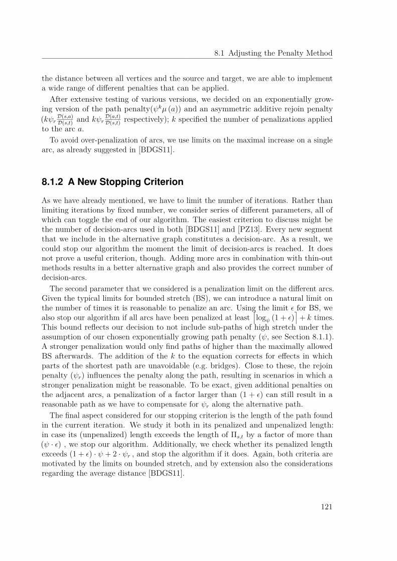
8.1 Adjusting the Penalty Method
the distance between all vertices and the source and target, we are able to implementa wide range of different penalties that can be applied.
After extensive testing of various versions, we decided on an exponentially grow-ing version of the path penalty(ψkμ (a)) and an asymmetric additive rejoin penalty(kψr
D(s,a)D(s,t) and kψr
D(a,t)D(s,t) respectively); k specified the number of penalizations applied
to the arc a.To avoid over-penalization of arcs, we use limits on the maximal increase on a single
arc, as already suggested in [BDGS11].
8.1.2 A New Stopping Criterion
As we have already mentioned, we have to limit the number of iterations. Rather thanlimiting iterations by fixed number, we consider series of different parameters, all ofwhich can toggle the end of our algorithm. The easiest criterion to discuss might bethe number of decision-arcs used in both [BDGS11] and [PZ13]. Every new segmentthat we include in the alternative graph constitutes a decision-arc. As a result, wecould stop our algorithm the moment the limit of decision-arcs is reached. It doesnot prove a useful criterion, though. Adding more arcs in combination with thin-outmethods results in a better alternative graph and also provides the correct number ofdecision-arcs.
The second parameter that we considered is a penalization limit on the different arcs.Given the typical limits for bounded stretch (BS), we can introduce a natural limit onthe number of times it is reasonable to penalize an arc. Using the limit ε for BS, wealso stop our algorithm if all arcs have been penalized at least
⌈logψ (1 + ε)
⌉+ k times.
This bound reflects our decision to not include sub-paths of high stretch under theassumption of our chosen exponentially growing path penalty (ψ, see Section 8.1.1).A stronger penalization would only find paths of higher than the maximally allowedBS afterwards. The addition of the k to the equation corrects for effects in whichparts of the shortest path are unavoidable (e.g. bridges). Close to these, the rejoinpenalty (ψr) influences the penalty along the path, resulting in scenarios in which astronger penalization might be reasonable. To be exact, given additional penalties onthe adjacent arcs, a penalization of a factor larger than (1 + ε) can still result in areasonable path as we have to compensate for ψr along the alternative path.
The final aspect considered for our stopping criterion is the length of the path foundin the current iteration. We study it both in its penalized and unpenalized length:in case its (unpenalized) length exceeds the length of Πs,t by a factor of more than(ψ · ε) , we stop our algorithm. Additionally, we check whether its penalized lengthexceeds (1 + ε) · ψ + 2 · ψr , and stop the algorithm if it does. Again, both criteria aremotivated by the limits on bounded stretch, and by extension also the considerationsregarding the average distance [BDGS11].
121

8 Engineering the Penalty Method
Algorithm 8.1 Penalty Method. This simplified illustration does not show the limitednumber of penalizations to a single arc.Input: A graph G (V, A) with associated metric μ, a source s and a target tOutput: An alternative graph H
1: H := P := Πs,t
2: D = L (P )3: G′ := applyPenalties(G)4: P ′ = Πs,t (G′)5: s = 0 � compare bounded stretch and decision-arcs6: while s < 10 and LG (P ′) ≤ (1 + ε) · D and LG′ (P ′) ≤ (ψ · (1 + ε) + 2ψr) · D do7: if isFeasible( Πs,t (G′) ) then8: s = s + 19: H := H ∪ Πs,t (G′) � include good paths in H
10: end if11: G′ := applyPenalties(G′) � further penalize the graph12: P ′ = Πs,t (G′)13: end while14: return H
8.1.3 Selecting Feasible Paths
As previously discussed, the usual approach to create an alternative graph initiallycomputes a series of penalized paths. Afterwards, a selection process is applied to triesand optimize Dtot and Davg. From the selected paths, all information – as far as wecan tell – is added to the alternative graph, potentially to be removed by thin-outmethods. In accordance to the quality criteria of Abraham et al. (see Definition 5.3),we propose the following method.
Instead of adding full paths to the alternative graph, we perform an evaluation andonly keep those parts that fulfil the criteria in Definition 5.4. Every path we findis divided into continuous segments. These segments are distinct from the currentalternative graph, except for their first and last vertex. We evaluate them for theirquality according to limited sharing and bounded stretch. We omit local optimality inthese considerations due to its incompatibilities with the penalization process.
We consider only segments that offer an alternative to a sub-path which is at leastfive percent of the shortest path in length. If, at the same time, their bounded stretchis less than twenty-five percent, we can add them to the alternative graph5.
The mathematical formulation of our criteria can be found Definition 8.1.
5In a commercial system, one might have to consider allowing longer detours in some special scenarioslike routes in Berlin for which no alternative routes would exist in comparison to the inner cityhighway.
122

8.1 Adjusting the Penalty Method
tsw
uv
(a) Intersection
s t
vu
(b) Join
Figure 8.1: Consideration of a path to use in an alternative graph. The left sideshows a segment that leaves the shortest path at u, crosses the alternative graphat v and joins it at w . On the right side, the path joins the corridor directly atv. By considering all segments between corridor vertices individually ((u, v) and(v, w) are treated separately of each other), we might end up keeping only the firstpart of the deviation for our alternative graph. The latter segment is discarded if itdoes not constitute a viable deviation on its own. As a result, both paths, thoughdifferent, could end up contributing the same to the alternative graph.
Definition 8.1 (Feasible Segment). A path segment, given as a sequence of arcs〈(v0, v1), (v1, v2), . . . , (vk−1, vk)〉 in relation to an alternative graph H with v0 ∈ H,vk ∈ H, and vj /∈ H , ∀j ∈ [1, k − 1]6 is feasible if the following conditions hold:
α · D (s, t) ≤ DH (v0, vk) (8.1)L (v0, . . . , vk) ≤ (1 + ε) · DH (v0, vk) (8.2)
The value for α describes the desire for limited sharing and is identical to the parameterin Definition 5.4. In the same way, ε is used to limit the bounded stretch.
We illustrate the concept of our Definition 8.1 in Figure 8.1. The main reason forthe common segments is that we want to provide a reasonable path to the target fromthe end of every segment. In a common vertex, there is always a reasonable way toswitch from one path to another.
Adding full paths to the alternative graph, rather than feasible segments, unneces-sarily increases the number of decision arcs. By using only viable segments, we avoidthe addition of unreasonably long and very minor detours. This restriction, however,reduces the value of Dtot that we can achieve. It is rather easy (compare Figure 8.4),however, to construct alternative graphs that contain unreasonable arcs which cansurvive both global and local thin-out. The problematic part in the thin-out methods isthat they only operate on the alternative graph alone. In our comparison, we considerthe full set of paths in the calculations and, as a result, prevent the insertion of sucharcs in the first place.
6(v0, v1) is also a valid segment, as long as the arc itself is not part of H.
123

8 Engineering the Penalty Method
Table 8.1: Impact on the average values for Dtot and Davg in dependence ofdifferent optimizations in our technique. Values specified consider random querieson the Berlin network (G8). We use an exponentially increasing scale along a path(factor 1.1) and asymmetric additive penalties (factor 0.002 D (s, t)).BS: stops if no further penalty was applied (all arcs penalized fully), limitedsharing (LS) adds only segments ignores short segments, LI limits the numberincreases on a single arc, μ stops the search if the last path without penalties is toolong, μπ does the same on the penalized path.
w/o thin-out thin-outset-up BS LS LI μ μπ Dtot Davg #arcs # alt Dtot Davg #arcs # alt
1 - - - - - 5.23 1.06 24.39 7.16 4.83 1.06 21.96 6.942 + - - - - 4.90 1.06 21.87 6.81 4.57 1.05 20.44 6.733 + + - - - 4.72 1.07 16.74 6.57 4.39 1.05 15.46 6.494 + + + - - 4.42 1.05 14.83 6.79 4.27 1.05 14.43 6.715 + + + + - 4.14 1.05 13.01 6.26 4.04 1.05 12.73 6.206 + + + + + 3.79 1.05 10.65 5.60 3.72 1.05 10.49 5.57
As a side note, our incremental approach allows to stop the algorithm early if acertain quality has been achieved. In our experiments, we always consider the full run,according to the previously mentioned stopping criterion, though.
8.2 Experimental Evaluation – Modifications
After the discussion of our modifications, we first take a look at how they affect thequality of the results. These considerations are mostly independent of running time ofa single customization.
8.2.1 Parameterization Influences.We have proposed a series of different ways to restrict the alternative graph in boththe number of iterations used and the segments that are added to it. None of thesemethods comes free, as can be seen in Table 8.1. In combination with Figure 8.2, wecan easily argue that the proposed changes still benefit our calculations. The reductionof Dtot by more than one over all the different set-ups can be justified by the increasein quality. While the last set-up does not exhibit any different behavior in our examplegraph, we found it to produce the best alternative graphs, based on visual appearance.
Without thin-out, our current set-up 6 may generate graphs with more than tendecision arcs. Using thin-out, set-up 6 stays within the limit, though.
The discussion based on the Berlin network is too restricted. Therefore, we alsostudied the effects of all the set-up variants on the western European road network
124

8.2 Experimental Evaluation – Modifications
(G1). In general, the observed changes remain the same. More restrictive set-ups lessenthe quality (Dtot) in a similar way. Therefore, the proposed changes remain valid.
Figure 8.3 indicates that our first restriction has the largest impact. As long as werestrict the calculations to viable segments of reasonable length, the further restrictionshave only a minor impact on the quality of the alternative graph. For most of thequeries, we can barely report a negative effect. Only extremely long queries can besaid to degrade in their quality. We notice a drop in quality from 4.5 to around 3.8 onaverage for the Dijkstra rank of twenty-four. On the other hand, the positive effect onthe number of decision arcs cannot be neglected.
In comparison to the values specified by Bader et al., we reach Dtot = 3.17 (Davg =1.04, # arcs = 7.2) on average compared to their value of Dtot = 3.34 on the samegraph. At the same time, our algorithm requires less than eight penalization iterationson average. While the values are a bit less, we think that the small decrease is wellwithin reasonable limits. If we perform a fixed number of twenty iterations, we canreach their values, as well.
8.2.2 Quality Considerations
Given the proposed adjustments to the alternative graph calculation, we need todiscuss their implications. A problematic finding in the penalty method, at least inour view, is the fact that, as illustrated in Figure 8.4, local detours of poor quality canincrease Dtot. Especially in subsections of the paths, this can become a problem. Thissetting is important to consider, as detours to a detour – even though reasonable whenconsidered as a whole – might be considered as too long, locally. Given that a pathcan be evaluated only with respect to the other arcs in the alternative graph, we couldeven generate local detours of near infinite relative length.
Therefore, it is difficult to fairly compare different approaches to the alternative graphproblem, as one can optimize for Dtot using such detours. In ignoring some connections,it is possible to increase the values of Dtot in a way that may be unreasonable.
In a direct comparison of the results of [BDGS11] and [PZ13], the improved qualityis most noticeable. As we see later on, the method we chose cannot produce a similarimprovement. In the following discussion, we provide arguments that justify why ourapproach is still reasonable, even though we only reproduce the results of [BDGS11].
The main reason for the differences in quality of our implementation and the one in[PZ13] is rooted in the different models of road networks. After a conversation withthe authors, we found that [PZ13] uses a model which we deem too simplistic for ourpurpose. The authors consider only three different road categories. In comparison,our network G1, which has been claimed to be realistic in [DGPW13], uses fifteencategories. They set highways to a travel speed of 130km
h, trunk roads7 to a travel
7According to the OpenStreetMap Wiki, trunk is a reference to the second most important roadcategory of a country.
125

8 Engineering the Penalty Method
(a) Set-up 1(b) Set-up 2
(c) Set-up 3 (d) Set-up 4
(e) Set-up 5 (f) Set-up 6
Figure 8.2: Exemplary evolution over the different set-ups of Table 8.1 for arandom route in the Berlin road network.
126
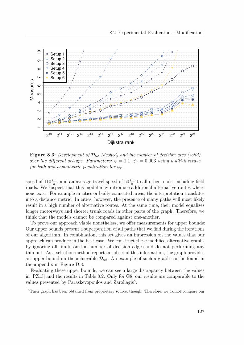
8.2 Experimental Evaluation – Modifications
●●
●●
●●
●●
●
●
●
●
●
●
●
●
●
●
●
● ● ● ● ● ● ● ● ● ●● ●
●
● ●
●
●
●
●
●
●
●
●
●
●
●
●
●
12
34
56
78
910
210 211 212 213 214 215 216 217 218 219 220 221 222 223 224
Dijkstra rank
Mea
sure
s
●
●
Setup 1Setup 2Setup 3Setup 4Setup 5Setup 6
Figure 8.3: Development of Dtot (dashed) and the number of decision arcs (solid)over the different set-ups. Parameters: ψ = 1.1, ψr = 0.003 using multi-increasefor both and asymmetric penalization for ψr .
speed of 110kmh
, and an average travel speed of 50kmh
to all other roads, including fieldroads. We suspect that this model may introduce additional alternative routes wherenone exist. For example in cities or badly connected areas, the interpretation translatesinto a distance metric. In cities, however, the presence of many paths will most likelyresult in a high number of alternative routes. At the same time, their model equalizeslonger motorways and shorter trunk roads in other parts of the graph. Therefore, wethink that the models cannot be compared against one-another.
To prove our approach viable nonetheless, we offer measurements for upper bounds:Our upper bounds present a superposition of all paths that we find during the iterationsof our algorithm. In combination, this set gives an impression on the values that ourapproach can produce in the best case. We construct these modified alternative graphsby ignoring all limits on the number of decision edges and do not performing anythin-out. As a selection method reports a subset of this information, the graph providesan upper bound on the achievable Dtot. An example of such a graph can be found inthe appendix in Figure D.3.
Evaluating these upper bounds, we can see a large discrepancy between the valuesin [PZ13] and the results in Table 8.2. Only for G8, our results are comparable to thevalues presented by Paraskevopoulos and Zaroliagis8.
8Their graph has been obtained from proprietary source, though. Therefore, we cannot compare our
127

8 Engineering the Penalty Method
s
t
u
v1
w
v2
45
45
1045
45
5
535
(a) Concrete example
s
t
u
v
x
0.2 · D (s, t)
D (s, t)
D (s, t)− x
0
(b) Theoretic construct
Figure 8.4: Illustration of a long local deviation along (u, w) and the influenceon Dtot. The graph using (u, w), ignoring (u, v1) and (v2, w) has Dtot equal to two.The other way around, we get Dtot equal to 1.95 . The second example is more ofa theoretical nature. It illustrates a scenario in which we can essentially generatean infinite local (x → 0) detour that, in terms of Dtot, remains a better choicethroughout the full process.
Using a distance metric on G8, we can increase the upper bound for Dtot to 7.8. In acomparison with their value (4.16 in [PZ13]), their method reaches fifty-three percentof the upper bound. Applying this same reduction to the other inputs, our algorithmprovides similar results on all graphs. Therefore, we compare ourselves to the qualityvalues presented in [BDGS11], even though they are lower than the ones in [PZ13].The comparison to other methods, both from the literature and our own methods,follow in Chapter 12.
algorithm on an identical data set.
128

8.3 Customizing a Single Query
Table 8.2: Upper bounds, consisting of all paths found within twenty penalizationiterations that are not more than twenty-five percent longer than the shortest path.This setting is comparable to the one chosen in [PZ13]. Values are calculated usingψ = 0.1 and ψr = 0.1 and the penalization described by [PZ13], using the sametype of queries (300 km limit). The comparison on the Berlin road network (G8)does not use an identical graph source. The graph in [PZ13] for this road networkis extracted from proprietary data. The number of first alternatives is specifiedwithout checks for LO. All reference values marked by an asterisk refer to differentdata sources or ones that were not defined closely enough in [PZ13].
w/o thin-out with thin outID Dtot Davg arcs # alt Dtot Davg arcs # alt [PZ13]G1 3.44 1.05 77.26 2.87 3.00 1.04 64.07 2.78 ∗5.24G2 3.64 1.05 83.06 3.37 3.19 1.04 70.41 3.26 ∗5.46G3 3.69 1.04 101.26 3.27 3.22 1.04 80.23 3.17 ∗5.24G4 4.63 1.05 125.03 5.13 4.17 1.05 103.37 5.00 5.46G5 3.37 1.04 64.90 2.56 2.94 1.04 50.61 2.48 -G6 4.28 1.05 95.02 4.34 3.82 1.05 77.14 4.22 -G7 3.64 1.05 55.27 3.60 3.21 1.04 43.34 3.51 -G8 4.14 1.04 34.26 4.36 3.72 1.04 26.31 4.28 ∗4.23G9 3.16 1.05 25.79 2.48 2.77 1.04 19.69 2.44 5.19
8.3 Customizing a Single Query
So far, we have seen that we can perform an iterative approach with an on-line stoppingcriterion. We already stated that our implementation is using CRP. We made thischoice, as CRP is used in commercial systems already (e.g. Bing Maps) and offerssome benefits in its structure. The distance matrices offer good cache locality and as aseparator-based approach, we can employ parallelism on independent parts.
In the following parts of this chapter, we discuss how we can achieve reasonableperformance on CRP, using parallelism, SSE, and some modifications to the generalstructure of CRP.
Cell Update Techniques. Before getting into the actual penalization, we have toexplore the update techniques we use for customization. [DGPW13] already considersdifferent techniques. Their road network model differs from ours, though; theirimplementation considers a turn-aware model. We chose to use the simple model overthe one incorporating turn-cost (compare [DGPW11, DGPW13, DW13]) to allow for abetter comparability to the other alternative route techniques. This choice is validatedby the fact that the only turn-cost available to us are a penalization of u-turns. Sincewe use a different model, we cannot simply rely on their measurements for our selection.
129

8 Engineering the Penalty Method
(a) Input Format (b) Relevant Result (c) Algorithm Progress
Figure 8.5: Schematic of our update algorithm based on the Floyd-Warshallalgorithm.
Since we update cells very often, optimal customization performance is critical.Next to the previously known techniques, we also added an additional one to therepertoire of available methods based on the Floyd-Warhsall algorithm. For ourmodified version, we make use of the vertex mapping already present for the CRPalgorithm (c.f. Figure 8.5a).
When we compute the distance matrix, most parts of the information are irrelevantto our progress. The vertex labelling we described puts the desired results in the top leftcorner of the matrix (c.f. Figure 8.5b). Our optimized version of the Floyd-Warshallalgorithm is tailored to this setting. We make use of this fact in progressing (c.f.Figure 8.5c) from the bottom right corner of the matrix to the top left. As long asthe considered via-vertex is not part of the output, we discard its respective row andcolumn of the matrix. This way, we reduce the future workload in every iteration.
The correctness of this approach follows from a contraction argument: our imple-mentation implicitly contracts all non-border vertices. Among the remaining vertices,we use the usual implementation of the Floyd-Warshall algorithm.
Using the distance matrices, the algorithm can be implemented by limiting i and j(see Algorithm 2.4) to the maximum of |C| , k in every iteration. This does not affectthe asymptotic running time, which is still O (n3), but the actual running time. Forfurther speed-up, we use vector instructions.
8.3.1 Omitting Origin and Destination Cells.
The cells that require an update can be calculated via a simple traversal of the extractedpath. We trigger an update for every cell on the bottom level that contains a vertexfrom the shortest path. These updates can be performed completely independently andin parallel. Iteratively, we mark the parent cells of the just updated cells and continuein the same way until all updates have been performed. Pseudo-code for the algorithmcan be found in the Appendix (Algorithm D.1).
130

8.3 Customizing a Single Query
(a) The path (b) Level zero (c) Level one (d) Level two
Figure 8.6: Illustration of the steps from a shortest path between a source anda target in CRP and the results of our dirty-cell computation with a maximalconsidered level of one in a three level CRP. The levels are marked zero, one, andtwo. Dirty cells are marked in red, non-dirty cells are marked in green.
In this process, we can omit updating the cells containing the source and the target(see Figure 8.6) at the cost of a minor modification to the query. The reasoning inthis approach is, that for the most part a query does not cross a cell multiple times.Imagine the search space that grows in a circle around the source. Omitting these twocells on every level (compare Figure 8.6), we enter a trade-off between the performanceof the query and the customization cost.
To preserve correctness, we need to descend both into the direction of the sourceand the target. Figure 8.7 gives an example of a query that cannot use the usuallevel as the full cell containing the source has not been updated. By descending intoboth the direction of the source and the target, we prevent the algorithm from using anon-updated cell.
The query is slowed, however, if we have to cross a cell. These cases, however, arerare and do not affect the query in a noticeable way. The rather large cost for updatinga cell easily compensates for the small additional query overhead.
Next to this optimization, we can even go one step further and omit full levels inthe query and update process.
Dynamic Max Level Selection. CRP itself is optimized to allow long-range queries.For short to mid-range shortest paths, higher levels will not be touched. They are,however, necessary for the optimal performance on transcontinental shortest-pathqueries. The correctness of the algorithm itself, however, does not require to useall computed levels. Instead, it can be restricted to any subset of them. Due tothe iterative process of path computation and penalization, we can utilize knowledgeabout the shortest path itself in our algorithm. This is substantially different from ausual shortest-path query in which the information only becomes apparent when thecomputation is finished. In our case, we can use the structure of the shortest path toadapt the behavior of our algorithm during its execution. By analysing the number ofhops of an average query of a given Dijkstra rank, we are able to select an appropriate
131
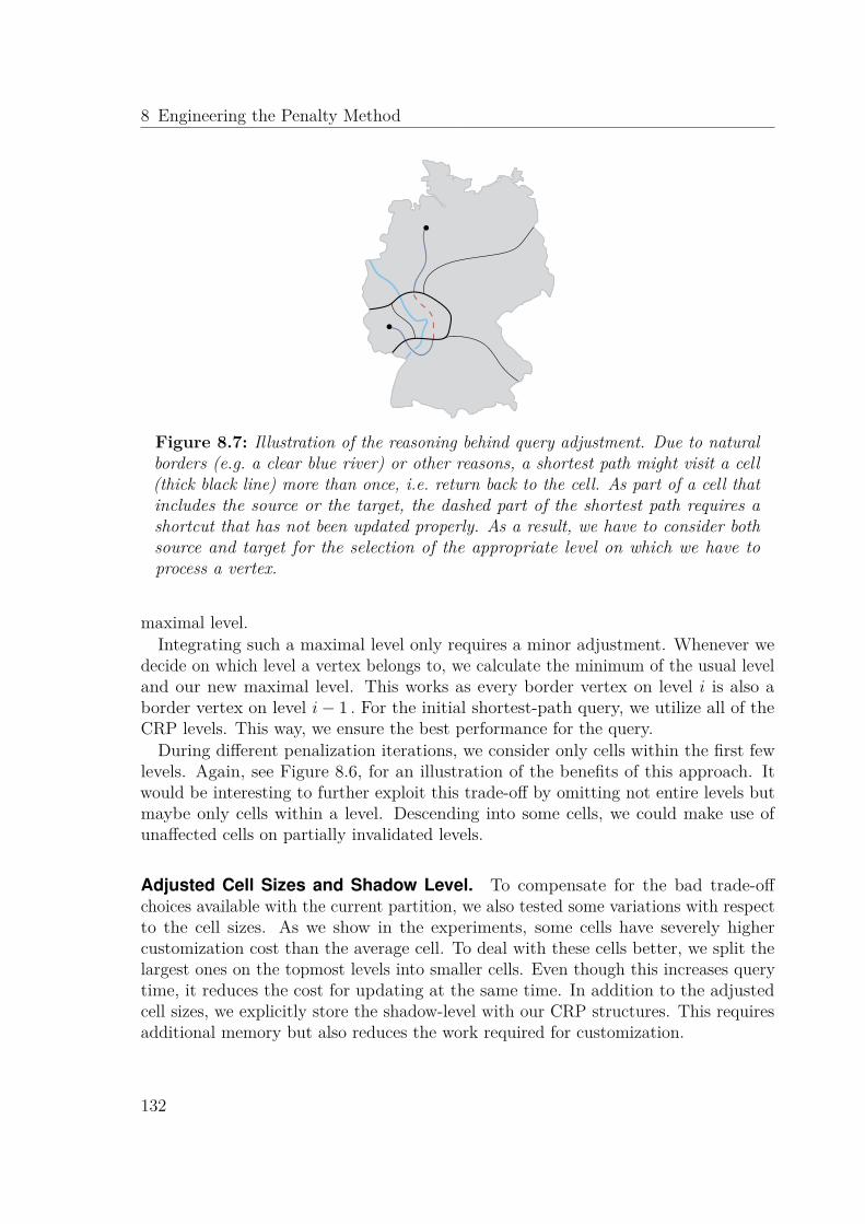
8 Engineering the Penalty Method
Figure 8.7: Illustration of the reasoning behind query adjustment. Due to naturalborders (e.g. a clear blue river) or other reasons, a shortest path might visit a cell(thick black line) more than once, i.e. return back to the cell. As part of a cell thatincludes the source or the target, the dashed part of the shortest path requires ashortcut that has not been updated properly. As a result, we have to consider bothsource and target for the selection of the appropriate level on which we have toprocess a vertex.
maximal level.Integrating such a maximal level only requires a minor adjustment. Whenever we
decide on which level a vertex belongs to, we calculate the minimum of the usual leveland our new maximal level. This works as every border vertex on level i is also aborder vertex on level i − 1 . For the initial shortest-path query, we utilize all of theCRP levels. This way, we ensure the best performance for the query.
During different penalization iterations, we consider only cells within the first fewlevels. Again, see Figure 8.6, for an illustration of the benefits of this approach. Itwould be interesting to further exploit this trade-off by omitting not entire levels butmaybe only cells within a level. Descending into some cells, we could make use ofunaffected cells on partially invalidated levels.
Adjusted Cell Sizes and Shadow Level. To compensate for the bad trade-offchoices available with the current partition, we also tested some variations with respectto the cell sizes. As we show in the experiments, some cells have severely highercustomization cost than the average cell. To deal with these cells better, we split thelargest ones on the topmost levels into smaller cells. Even though this increases querytime, it reduces the cost for updating at the same time. In addition to the adjustedcell sizes, we explicitly store the shadow-level with our CRP structures. This requiresadditional memory but also reduces the work required for customization.
132

8.4 Experimental Evaluation
Cleaning Up. Due to the modifications we make to CRP during the penalization, wehave to do some maintenance work after the query. We do this by simply keeping a listof dirty cells for every level. When we modify a cell for the first time, we simply replacethe pointer in the data structure that points to the (now) modified cell. The originalpointer is remembered with the list of dirty cells. When our algorithm concludes, wesimply traverse this list and restore the original data structures for CRP. This preventsa final customization on the dirty cells.
8.3.2 Alternative Route Extraction
To allow a comparison to other techniques, we also extract paths from the graph.We extract paths by employing X-BDV9). Given the small size of the graph, theperformance is good enough and can be neglected in comparison to the construction ofthe graph itself. Some checks, however, cannot be performed in the restrictive settingof an the alternative graph. Especially the check for local optimality (LO) does providereasonable results, if we do not consider the full graph. Therefore, we can only assumethe different segments of the graph to be reasonable and not rely on the LO check.Our evaluation on the full graph show that this assumption can be made, though.
Further Potential. The available parallelism has some potential for further improve-ments, still. The trade-off between the number of levels to customize and the querytime is currently only partially exploited for its parallelism. For example one couldemploy Δ-stepping to hasten the execution. The large matrices increase the degree ofthe traversed vertices, next to the creation of longer arcs, which lend themselves to aparallel implementation via Δ-stepping, for example. In addition, we could parallelizethe individual tasks during the path extraction. We could also add goal direction tosubsequent queries by restricting the search to cells that allow for low stretch routesto be found in the first place. Finally, we assume that there are different partitioningschemes we could implement to even better exploit the trade-off between query andpenalization performance.
8.4 Experimental Evaluation
After our initial consideration with regards to the penalization scheme, we now discussthe performance of different iterations. At this point, we focus purely on parametertuning an efficiency. Our experiments use a partition of the European road network(PTV) created by Punch [DGRW11]; the properties of the partition are summarized inTable 8.3. It was kindly provided by Daniel Delling. The partition is similar to theone used in the initial contribution of Delling et al. [DGPW11].
9The complete plateau method, see Section 5.2.
133

8 Engineering the Penalty Method
Table 8.3: Overview of the partition used in our experiments to the penalty method.A graphical illustration of the partitions can be found in the Appendix (Figure A.2).
level vertex limit cells size border vertices border-arcsavg max avg max
0 25 664 300 27.1 5.2 21 5.3 241 28 82 278 218.9 10.0 55 9.7 442 212 5 046 3 569.2 26.4 96 24.9 933 216 319 56 458.2 67.9 208 63.4 2054 220 20 900 509.0 136.8 384 126.2 361
The level zero is commonly referred to as the shadow-level. For our purposes, weconsider two variants of the CRP algorithm. The first one considers all levels, storingthe distance matrices explicitly, even for the shadow-level; we refer to this variant asCRP-4S which is essentially a five level variation of CRP. In the second variant, weonly use levels one through four; this variant is named CRP-4. This version only usesthe shadow-level to guide the creation of the microcode.
For customization, we tested a series of different methods from [DW13] as well as ourpruned Floyd-Warhsall implementation, summarizing the results in Table 8.4. In thesimple model, our microcode customization only performs best for the first level, nomatter whether we study CRP-4 or CRP-4S. Surprisingly, on the first level of CRP-4S,our tuned Floyd-Warhsall implementation manages to outperform all other variants.From level two on upwards, the Bellman-Ford implementation performs best. For ourupdate methods, we select Microcode for the first level of both CRP-4 and CRP-4S.For the topmost three levels, we select the SSE tuned implementation of Bellman-Ford.Finally, we select our tuned implementation of the Floyd-Warshall algorithm for levelone of CRP-4S. This does not only speed-up our algorithm but also saves memoryconsumption in comparison to the microcode for the minor cost of a few lines of code.
Both settings offer comparable running times, when we perform a full update. Thelarger flexibility in updating only parts of a cell on the bottommost level, led us tochoose the version that incorporates the shadow layer for all further processing, though.
8.4.1 Penalization
Penalizing a path in CRP requires the update of multiple cells on different levelsof the hierarchy. Figure 8.8 summarizes the affected cells in our partition of theWestern-European road network. Short-range queries only affect very few cells – belowa tenth of a percent for the bottommost level. For long-range queries and higher levels,this percentage increases significantly. For example, a long-range query covers morethan twenty percent of the topmost cells.
In combination, Figure 8.8 and Table 8.4 indicate that updating all levels might be
134

8.4 Experimental Evaluation
Table 8.4: Update cost on different levels of the CRP hierarchy for various tech-niques in our implementation. The maximal value specifies the 99% quartile tocorrect for measuring errors. Levels two through four are the same for both CRP-4and CRP-4S and their measurements are given in [ms]. The former levels specifytimes in [μs]. The Microcode for levels three and four is omitted due to its largesize and decreasing benefits. The values represent a single customization.
level Dijkstra Bellman-Ford Floyd-Warshall Microcodeavg max avg max avg max avg max
0 6.84 18.16 3.49 9.75 2.17 3.62 1.16 4.371 22.09 83.33 11.61 42.77 8.01 30.33 8.28 43.98
0+1 132.04 356.56 80.89 273.17 74.83 143.97 11.03 43.422 0.25 1.12 0.13 0.56 0.13 0.71 0.17 1.073 2.07 10.72 1.10 5.46 2.02 12.08 - -4 16.89 62.43 11.96 39.24 33.58 103.11 - -
infeasible. Even though the average case behaves quite well, the maximal time spentupdating a single cell is very expensive.
Pruning source- and target cells. When customizing CRP, the most work is donein the lower levels. As we just argued, the distribution of workload shifts to higherlevels when only considering a single path, though. In our scenario, the update costsfor cells on higher levels are considerably larger than those of lower levels. Figure 8.9aillustrates the cost for the penalization of a single path. It can be seen that in thestandard CRP model, even the penalization of a single path can be too expensive. Theunmodified customization would not even allow for a single iteration in our setting.
The proposed pruning of the source and target cells can hasten the short-rangequeries, though. As illustrated in Figure 8.9b, we can decrease the cost of an iterationfor Dijkstra ranks up to 220 to less than ten milliseconds on average. This can beachieved by not updating those cells that are only required for long-range queries.Compare Figure 8.10 for an illustration of the full benefits. Longer-range queries,however, still suffer from the high update cost of some of the top-level cells.
For the most interesting queries this modification already allows for a sufficientnumber of iterations to compute a viable alternative graph, given the amount ofiterations we require. We study the possible trade-off between query-performance andcustomization overhead by reducing the number of used levels in the next section.
Maximum Level Selection. Extracting paths from CRP is expensive, compared toan algorithm like CH. Each extraction process has to recursively find the arcs thatcontribute to a shortest-path segment in the lower level (c.f. Figure 8.11b). When
135

8 Engineering the Penalty Method
●●
●●
●●
●●
●●
●●
●●
●
● ● ● ●
●●
●
● ●
●
●
●
●
●
●0.
001
0.01
0.1
110
210 211 212 213 214 215 216 217 218 219 220 221 222 223 224
Dijkstra Rank
Affe
cted
Cel
ls [%
of l
evel
]
●
●
Level 0Level 1Level 2Level 3Level 4
Figure 8.8: Affected cells on the different CRP-hierarchy levels for the Western-European road network (PTV) and the previously discussed partition. This plotalready incorporates the optimization to omit the cells that contain either the sourceor the target.
we limit the number of levels used during the query, the query itself is undergoing aslowdown while, at the same time, the extraction process is hastened. In combination,this directly translates into a near equivalence of the settings using all levels and asetting that completely ignores the topmost one. Taking the cost for the customizationprocess into account, it becomes apparent that the topmost level can be ignored duringthe penalization process. It only adds a slight benefit during the initial shortest-pathcomputation10.
It turns out that the query itself is far more sensitive to the level selection process thanthe path extraction (c.f. Figure 8.11). Our measurements indicate that a restrictionto the two lowermost levels is viable up until approximately Dijkstra rank 215. Theaddition of the third level is enough up to Dijkstra rank 222, and only very longlong-range queries require four levels.
The overall process, however, is a bit more complicated. As a result of the interactionbetween the update costs, the query, and the path extraction, we are required to takea look at the whole picture. The only obvious fact, so far, is that the costs for the10It is possible to hasten the extraction process by adding some flags that indicate whether an arc in
a cell of level i is part of an arc in level i + 1. In the dynamic nature of our algorithm, these flagswould add a considerable customization overhead, though.
136

8.4 Experimental Evaluation
Dijkstra Rank
Tim
e [m
s]0.
010.
11
1010
0
210 211 212 213 214 215 216 217 218 219 220 221 222 223 224
Level 0 Level 1 Level 2 Level 3 Level 4 Others
(a) All cells updated.
Dijkstra Rank
Tim
e [m
s]0.
010.
11
1010
0
210 211 212 213 214 215 216 217 218 219 220 221 222 223 224
Level 0 Level 1 Level 2 Level 3 Level 4 Others
(b) Source- and target-cells pruned.
Figure 8.9: Cost of a single iteration, depicting the accumulated time to update allcells of a given path up to the specified level as well as the additional cost associatedwith the respective CRP query and administrative overheads. Dijkstra rank onethrough ten are omitted for readability.
137

8 Engineering the Penalty Method
Dijkstra Rank
Spe
ed−u
p
● ● ● ● ● ● ● ● ● ● ● ● ● ● ●
● ●
●● ●
●
●
●
●
●
110
100
210 211 212 213 214 215 216 217 218 219 220 221 222 223 224
● ●Level 0 Level 1 Level 2 Level 3 Level 4 Total
Figure 8.10: Speed-up of penalization: pruned source- and target-cells over allcells updated.
lowest two levels are negligible for longer-range queries. In total, we spent around threemilliseconds on them.
In Figure 8.12 we illustrate the cost and the possible count of iterations for animplementation that considers only a certain subset of levels. Considering the full costof an iteration, it seems that a maximum of three levels performs best. The updatecost for the fourth level already outweighs the benefits during the query. Including thecost for the penalized query and all book-keeping overhead, the introduced methodsalready allow for alternative graph computations of queries up to Dijkstra rank 220 .This is under the assumption of about ten rounds of penalization. For the largestDijkstra rank, the sequential execution allows for a single round of penalization. Asingle penalization might already suffice to find an alternative route to a shortest path.
The independent parts of the computation allow for a parallel execution of thealgorithm. Using multiple cores, we can increase this limited count of possible iterationsto achieve a full implementation of the penalty method.
8.4.2 Parallel Execution
In combination, Table 8.4 and Figure 8.8 indicate that the query itself might be thebottleneck of each iteration. Especially when we use fewer levels, compare Figure 8.11a,the query dominates the effects of parallel-executed customization. If we use more levels,
138

8.4 Experimental Evaluation
●●
●●
●●
●●
●●
●●
●● ●
●●
●
●
●
●
●
●
●
●
●
●
●
●●
0.01
0.1
110
100
1000
210 211 212 213 214 215 216 217 218 219 220 221 222 223 224
Dijkstra Rank
Tim
e [m
s]
●
●
5 Levels4 Levels3 Levels2 Levels1 Level
(a) Query
●●
●●
●●
●●
●●
●●
●●
●
●●
●● ● ●
● ●●
●●
●●
●
●
0.01
0.1
110
100
1000
210 211 212 213 214 215 216 217 218 219 220 221 222 223 224
Dijkstra Rank
Tim
e [m
s]
●
●
5 Levels4 Levels3 Levels2 Levels1 Level
(b) Extraction
Figure 8.11: Query and extraction cost of a CRP query on G1 when limitingthe algorithm to operate only on a subset of levels. The legend shows the ID ofthe topmost level that was used during the query. Optimizing the extraction mightspeed-up the overall process. It remains unclear, though, how to achieve this in ourdynamic setting.
139
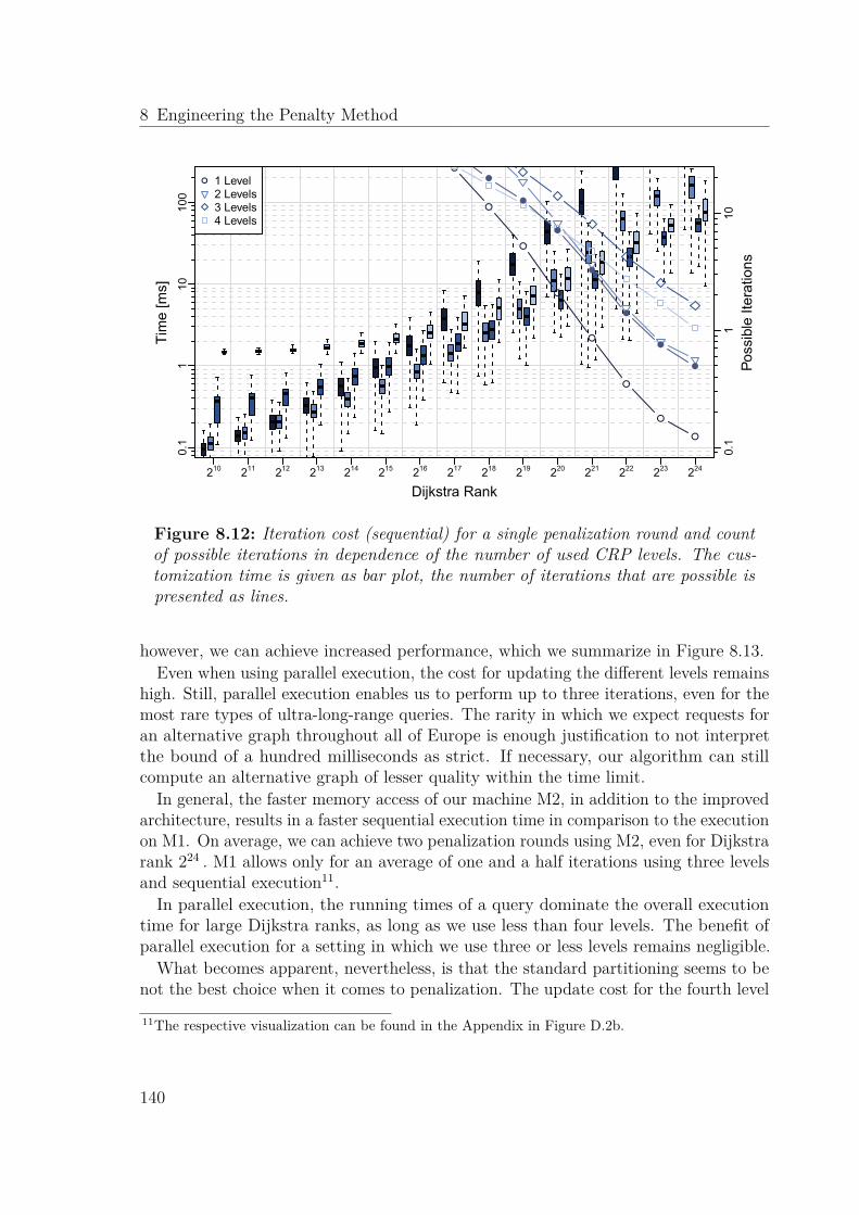
8 Engineering the Penalty Method
0.1
110
100
●
●
●
●
●
●
●
●
●
●
●
●
●
●
●
0.1
110
210 211 212 213 214 215 216 217 218 219 220 221 222 223 224
● 1 Level2 Levels3 Levels4 Levels
Dijkstra Rank
Tim
e [m
s]
Poss
ible
Iter
atio
ns
Figure 8.12: Iteration cost (sequential) for a single penalization round and countof possible iterations in dependence of the number of used CRP levels. The cus-tomization time is given as bar plot, the number of iterations that are possible ispresented as lines.
however, we can achieve increased performance, which we summarize in Figure 8.13.Even when using parallel execution, the cost for updating the different levels remains
high. Still, parallel execution enables us to perform up to three iterations, even for themost rare types of ultra-long-range queries. The rarity in which we expect requests foran alternative graph throughout all of Europe is enough justification to not interpretthe bound of a hundred milliseconds as strict. If necessary, our algorithm can stillcompute an alternative graph of lesser quality within the time limit.
In general, the faster memory access of our machine M2, in addition to the improvedarchitecture, results in a faster sequential execution time in comparison to the executionon M1. On average, we can achieve two penalization rounds using M2, even for Dijkstrarank 224 . M1 allows only for an average of one and a half iterations using three levelsand sequential execution11.
In parallel execution, the running times of a query dominate the overall executiontime for large Dijkstra ranks, as long as we use less than four levels. The benefit ofparallel execution for a setting in which we use three or less levels remains negligible.
What becomes apparent, nevertheless, is that the standard partitioning seems to benot the best choice when it comes to penalization. The update cost for the fourth level
11The respective visualization can be found in the Appendix in Figure D.2b.
140

8.4 Experimental Evaluation0.
11
1010
0
●
●
●
●
●
●
●
●
●
●
●
●
●●
0.1
110
210 211 212 213 214 215 216 217 218 219 220 221 222 223 224
● 1 Level2 Levels3 Levels4 Levels
Dijkstra Rank
Tim
e [m
s]
Poss
ible
Iter
atio
ns
Figure 8.13: Parallel penalization on G1, using twenty-four threads on M2. Thecustomization time is given as bar plot, the resulting number of possible iterationsis presented as lines.
is too high, as the amount of cells that can be updated in parallel is too low. For threelevels and less, the query time is dominant.
Adjusted Cell Sizes. Figure 8.14 illustrates that splitting large cells provides abetter trade-off than previously observed. Even in sequential execution, using fourlevels is already faster than the the setting using only three levels for Dijkstra ranksbetween powers of twenty-two and twenty-four. Therefore, we chose to use thesemodifications to improve performance for larger Dijkstra ranks.
8.4.3 Final ConfigurationAs previously mentioned, after extensive measurements on different configurations, weselected ψ = 1.1 and ψr = 0.01 for our implementation of the penalty method. For thepenalization, we chose an exponential penalization of path arcs and an asymmetricadditive penalty applied once to all arcs adjacent to a (penalized) shortest path. Thechosen configuration provides the results illustrated in Figure 8.15. For our timingmeasurements, we present values measured on twenty-four threads, an amount ofthreads only required for peak performance. Measurements using only four threadsare barely slower. Most times, using only a few threads suffices. Further details onpossible configurations can be found in Appendix D.
141

8 Engineering the Penalty Method
0.1
110
100
●
●
●
●
●
●
●
●
0.1
110
210 211 212 213 214 215 216 217 218 219 220 221 222 223 224
● 1 Level2 Levels3 Levels4 Levels
Dijkstra Rank
Tim
e [m
s]
Poss
ible
Iter
atio
ns
Figure 8.14: Cost of a sequential penalization of G1 on M2 using a partition inwhich large cells have been split into four separate cells. Compare Figure 8.12 for asetting without this subdivision.
On random queries, we reproduce the values specified by Bader et al., reaching avalue of Dtot = 3.17 (Davg = 1.04, # arcs = 7.2) on average compared to their valueof Dtot = 3.34, which requires an average query time of a hundred milliseconds. Forshort-ranged queries (maximum of 300 km between s and t), we achieve Dtot = 2.23 inaround ten milliseconds. On these short-ranged queries, our Dijkstra implementationrequires an approximate eight milliseconds for a single run.
Given our additional restrictions on the paths and our online selection strategy, weare willing to accept this minor decrease in quality, compared to Bader et al.. All ofthese values can be tuned to provide even better quality (compare Figure 8.3, Set-up6); we deem this unnecessary, however, as the actual values depend strongly on theunderlying graph and especially the used metric.
We achieve near interactive query performance for the full range of Dijkstra ranks(Figure 8.15a).
Quality. In Figure 8.16, we illustrate the development of the different quality pa-rameters. The stretch of different paths increases slowly from short-ranged queries tolong-ranged queries. The amount of sharing (α) remains mostly constant at aroundfifty percent. The local optimality degrades from around ninety percent to aroundthirty percent. The distance between the points offering the largest values for bounded
142

8.4 Experimental Evaluation
Dijkstra Rank
Tim
e [m
s] /
Itera
tions
● ● ● ● ● ● ● ● ● ● ● ● ● ● ●
0.01
0.1
110
100
210 211 212 213 214 215 216 217 218 219 220 221 222 223 224
●
InitUpdateQueryAGCTotalIterations
(a) Timing (M2)
● ●● ●
●● ● ● ● ●
●●
● ● ●● ● ● ●
● ●
●
●●
●●
●
●
●
●
●
●
●
●
●
●●
●●
● ●●
●● ●
● ● ●
01
23
45
67
89
10
010
2030
4050
6070
8090
100
21 22 23 24 25 26 27 28 29 210 211 212 213 214 215 216 217 218 219 220 221 222 223 224
Dijkstra Rank
Mea
sure
s
Suc
cess
Rat
e [%
]
●
●
totavgalts#dec. arcssuccess
(b) Quality
Figure 8.15: Final evaluation of our implementation of the penalty method, usingψ = 1.1 and ψr = 0.01 . The quality specified depicts average values with respect tothe successfully executed calculations (Dtot > 1). Figure 8.15a provides accumulatedtimings for the initial query (init), updates (penalization and customization), re-peated queries (query) and the construction of the actual alternative graph (AGC).In addition, we depict the average number of iterations performed as well as thetotal time taken for our algorithm.
143

8 Engineering the Penalty Method
●
● ●
●●
● ●● ● ● ●
● ● ● ● ●● ●
● ●●
●
●
●●
●
●
●
●
●
●●
●
●
● ● ●
●● ●
●
●●
●● ●
010
2030
4050
6070
8090
01
23
45
67
89
10
21 22 23 24 25 26 27 28 29 210 211 212 213 214 215 216 217 218 219 220 221 222 223 224
Dijkstra Rank
Para
met
er V
alue
● ●α β ε ε−base success #alt δtot
Figure 8.16: Development of quality for Customizeable Route Planning withPenalization (CRP-π) over different path lengths
stretch (ε) behave in the same way. Dtot increases slowly, peaking at a Dijkstra rank of223. The number of first alternatives follows this development, not dropping of at rank224, though.
8.5 Conclusion
Even though it seemed unlikely at first, the penalty method can be implementedefficiently. In our studies, we thoroughly explored the different trade-offs associatedwith an implementation on the basis of CRP and were able to configure the algorithm toour specific goals. We refer to our highly tuned implementation as CRP-π. Exploitingthe initial shortest-path search, we can dynamically adjust our technique to handleevery possible scenario in the most reasonable way possible. Our final result offers atechnique that is comparable to the results of Bader et al. [BDGS11] in its quality andcan handle close to any query type within or at least close to a hundred milliseconds.
The mentioned optimization potential for further parallelism could result in evenbetter performance. Also, tuning the partition further to fit the desired purpose evenbetter might prove beneficial. The formerly mentioned radix heap could prove beneficialas a replacement for the utilized binary heap. Finally, also the query itself offers somepotential for parallelization. While we found the parallel execution of both forwardand backwards search to be subject to too much synchronization overhead to justify
144

8.5 Conclusion
the implementation, introducing Δ-stepping could offer a large potential for furtherexploitation of parallelism. Ours is the only implementation of the penalty methodsuited for interactive applications, even on continental-sized road networks.
145

9 Chapter 9
A new Approach toVia-Alternatives
This chapter presents a different approach to the calculation of via-alternativesand alternative graphs in general. We present the first speed-up technique basedalgorithm that directly computes a full alternative graph, rather than evaluatinga series of path candidates. Our algorithm requires a single bidirectional queryto succeed and offers high quality alternative routes in a competitive amountof time. This chapters describes the single-author publications [Kob13].
The most common approach for the calculation of alternative routes, so far, is thevia-vertex appraoch. The algorithms presented by Abraham et al. [ADGW13] as wellas an extension due to Luxen and Schieferdecker [LS12] both operate in a similarfashion. After selecting a via-vertex candidate in a heuristic fashion, the vertex istested for admissibility and selected on success. The ordering heuristic approximatesthe quality of an alternative route based on shortcuts. The test itself requires threeshortest-path queries. Therefore, both methods present the first viable alternative pathas a result instead of evaluating all candidates.
The discovery of candidates is one of the major parts of both algorithms. Abrahamet al. require a relaxed pruning mechanism to achieve reasonable success rates. Theyrelax the pruning mechanism by allowing the query to descend within the hierarchy.This descend is controlled via the levels of up to k parent vertices1. The relaxationnot only increases the success rate. The highly increased number of candidates alsoincreases the workload of the algorithm during its testing phase.
Luxen and Schieferdecker follow a different approach and build an alternative routecover for all vertices within pairs of distinct regions. Their algorithm employs theclassical algorithm of Abraham et al. [ADGW13] as a base case to detect possiblealternative routes. Every discovered viable candidate is remembered in relation to theregions of the source and the target. For every query, their algorithm first explores
1Google recently patented a method [Gei14] that might improve this mechanism.
147

9 A new Approach to Via-Alternatives
these stored candidates. If a previously found vertex offers a viable candidate, thevertex is reported as via-vertex. Else, the method uses the algorithm of Abrahamet al. to find new candidates. In combination with the Arc-Flags (ArcFlags) algorithm,[LS12] offer the currently fastest algorithm for the discovery of alternative routes.
One point of critique, in our eyes, is the sequential evaluation of different candidatesthat reports the first viable via-vertex. We think that the heuristic selection ofcandidates might negatively impact the route quality. In this chapter, we develop analgorithm that can test all its candidates at once. Even though we require a largerinitial overhead, the simultaneous tests results in competitive running times to themethod of Abraham et al..
Our method borrows ideas from PHAST [DGNW13] and [LS11] to calculate analternative graph on top of a single bi-directional shortest path query. The methoddoes not require additional relaxation. The basic principles are comparable to themethod presented in [Cam05]. Instead of using Dijkstra’s algorithm, however, we useCH.
9.1 Alternative Graphs via Plateaux
Previous techniques for alternative routes all follow an iterative approach; they computea single path at a time. Surprisingly, even techniques that focus on the discoveryof full graphs [BDGS11, PZ13] calculate a series of paths. The only exception isChoice Routing [Cam05] and the reference algorithm X-BDV of Abraham et al. (seeSection 5.2).
Both techniques require Dijkstra’s, though, which is too slow for long-range queriesin an interactive setting. We improve upon Choice Routing and X-BDV by applyingtheir concept, i.e. the discovery of plateaux, to Contraction Hierarchies. By testing allcandidates in a single bi-directional query, we are unique among all (speed-up techniquebased) algorithms designed to compute alternative routes.
Our approach operates in three different steps.
Shortest-path Trees The first step computes two (partial) shortest-path trees. Sincewe are using a CH, these trees consist mostly of shortcuts.
Hierarchy Decomposition As in [LS11], we collapse the hierarchy of the CH. Thisphase discovers the plateaux and prepares our alternative graph.
Post Processing In a final step, we process the graph to contain less unnecessarydata.
The first step is a bi-directional query that computes two shortest-path trees. As inX-BDV, the intersection of these trees defines so-called plateaux, which can be usedto perform the T-test for local optimality (see Section 5.2.1). Rather than evaluating
148

9.1 Alternative Graphs via Plateaux
single plateaux for alternative routes, we construct a full graph that maintains all theinformation required for alternative route extraction.
Speed-up techniques in general are optimized for point-to-point queries. For CH,however, techniques exist that compute full and partial shortest-path trees [DGW11,DGNW13]. Both techniques use an initial upward search in combination with a sweep.PHAST processes all vertices, Restricted PHAST (RPHAST) a precomputed subset ofthe vertices. For our approach, we cannot compute these vertices in advance but haveto identify them. We describe our approach to this problem in Section 9.1.1.
By using a CH, we face the same problem as the classical via-vertex approach. Thetrees found in the first step contain a lot of shortcuts. Within these shortcuts, some ofthe required plateaux can be hidden. Our second step in the algorithm processes thesetrees, extracting all shortcuts to discover the plateaux.
Collapsing the hierarchy can be a costly operation. In fact, this step containsthe largest part of the workload. As the most costly part of the algorithm, it alsoprovides the name for our algorithm: Hierarchy Decomposition for Alternative Routes(HiDAR). The process is difficult, not only because the amount of arcs represented bythe shortcuts is large. In addition, even at first glance fully unrelated shortcuts canshare a common segment.
This step, similar to the usually employed relaxation, is only a heuristic, though.We cannot guarantee the discovery of all viable via-vertexs. The heuristic is very good,though, and misses fewer vertices than the usual relaxation. In comparison to X-BDV,we cannot offer the same success rates, though. We narrow the gap to the referencealgorithm, though.
Finally, the last part of our algorithm performs post-processing on the computedalternative graph.. This step is independent of the alternative route extraction algorithmand reduces the size of the alternative graph. We both compress and filter the graph,based on some information computed in step two, without actually touching all verticesa second time. The graph that we construct provides all information required toperform a quick evaluation of alternative route viability with respect to the criteria setforth by Abraham et al. (see Definition 5.4).
9.1.1 Building Shortest Path TreesThe first step of Hierarchy Decomposition for Alternative Routes (HiDAR) is thecomputation of two shortest-path trees. For our algorithm to perform well, we need torestrict the trees to a reasonable subset between the two extremes: a full shortest-pathtree and a point-to-point query.
In the decision process, we performed some initial experiments using the algorithm ofAbraham et al. [ADGW13]. The experiments revealed that all viable via-vertexs wereactually contained within one of shortcuts of either the source or the target. While wecannot guarantee this in general, the measurements justify our approach to calculatefull shortest-path trees for the union of search spaces of the source and the target.
149

9 A new Approach to Via-Alternatives
Due the the large overall size of all possible search spaces, we cannot computethe search space of all vertices in advance, as done for RPHAST [DGW11]. In ouralgorithm, we combine the discovery of the vertices with the initial upward search.
1. Upward Search and Sweep Space Generation. Both the generation of thesweep space and the initial distance computations traverse the graph in an upwardsfashion. We can exploit this identical mode of operation and combine both into a singleparse. Whereas we require Dijkstra’s algorithm to compute distances in a generalgraph, we can utilize a different order of processing in a CH. Since the search is directedupwards, we can order the vertices with respect to their level in the CH 2.
Theorem 9.1 (Correctness of the Upward Search). Processing the vertices in order oftheir CH-level does not influence the distance calculation.
Proof. Similar to the correctness of PHAST, we can employ an inductive argument.Whenever a vertex v is processed on level �, its distance is correct and all arc relaxationsuse a correct distance value. The source offers the base case with a correct distance ofzero. The distance of a vertex v on level � depends only on vertices at level � − 1 andsmaller. The inductive argument claims them to be assigned a correct distance value.As a direct result, the distance value of v is also correct.
Naturally, this correctness argument only holds with respect to the search spaceof the CH. An alternative argument would be that a breadth-first search (BFS) cancompute correct distance values in a weighted DAG, as well.
Using the CH level as ordering criterion, we can compute both all reachable verticesand the initial distance values at the same time, saving an additional parse over thevertices. The exact process is described in Algorithm 9.1. We describe it the wayit works starting at the source. The algorithm works the same way from the target,though.
During the upward search on the forward graph, we add additional vertices to thequeue. All vertices that are reachable in the backward graph are added to the queuewith an infinite weight. When we process a vertex of infinite weight, we only considerthe backward graph for relaxation.
The union of all touched vertices forms the set of vertices that we sweep in thesecond phase.
We can also employ some initial pruning at this point, throwing away all vertices forwhich the upward part already indicates a larger distance than 1 + ε times the bestknown value for D (s, t) so far. In doing so, we employ the usual stopping criterion ofa CH. The correctness of this approach follows directly from the correctness of a CHquery. Similar to the usual CH query, we advance the two searches simultaneously andkeep track of a tentative distance value for the full path.
2The level in a CH is defined as the number of hops from a vertex to the topmost vertex.
150

9.1 Alternative Graphs via Plateaux
≺
s s s
(a) Classic
≺
s s s
(b) Bucket
Figure 9.1: Changed operation order: the top row shows a schematic of the classicorder that uses a priority queue to calculate distances within the search space ofthe source s. The bottom row shows our operation order that processes the searchspace of s in a per-level fashion. Due to the full exploration of the search space, wegain no benefit from the priority queue based ordering.
The method proposed seems promising as we do not require the ordering capabilitiesof a priority queue for the vertices, perform only a single parse over the search spaceand still do not lose much in terms of pruning potential over the standard CH query.
Formally speaking, the result of this initial phase, when starting at the source,consists of all vertices that are reachable in the union of G↑ and G↓ from either sourceor target. This is different from the search space of Dijkstra’s algorithm as we searchbackwards in G↓; both searches only go up the hierarchy. In addition to the sweepspace, we perform the full initialization as done in PHAST or RPHAST.
2. Sweep. In the second phase, we can operate purely using the information gainedfrom the first phase. Exactly as in RPHAST, we can sweep the set of vertices that wehave computed in the previous step (RPHAST calculates the sweep sets in advance).This phase extends and corrects the tentative shortest-path trees found in the first stepof this phase. This second part, the sweep, concludes the first phase of our HiDARalgorithm.
Theorem 9.2 (Tree correctness). The query of HiDAR calculates two shortest-pathtrees.
Proof. The correctness is a direct implication of the correctness of RPHAST, the re-gional version of PHAST, in combination with the sweep space. As seen in Theorem 9.1,the modified upward search offers a correct initialization.
151

9 A new Approach to Via-Alternatives
Algorithm 9.1 ComputeShortestPathTreesAndSweepSpaceInput: A graph processed into a CH, a source s and a target tOutput: The shortest-path distances between s and all vertices reachable from the
source in G↑ and ∞ for all vertices reachable in G↓
1: Q [·] := ∅2: Q [� [s]] .push(s)3: distance[] = ∞4: distance[s] = 05: sweep = ∅6: for all level ≥ � [src] do7: for all v ∈ Q[level] do8: sweep.push(v)9: if distance[v] = ∞ then
10: for all (v, w) ∈ G↑ do11: distance [w] = min(distance[w], distance[v] + μ ((v, w))12: Q [� [w]] .push(w)13: end for14: end if15: for all (v, w) ∈ G↓ do16: Q [� [w]] .push(w)17: end for18: end for19: end for20: return (distance, sweep)
For the correctness of the sweep, we can directly use the proof for RPHAST whichrequires the full upwards search space of a vertex. Since we are extending the searchin G↓ from every vertex, this is obviously the case.
9.1.2 Discovering Plateaux
The second phase of HiDAR is concerned with the discovery of the different plateaux.The separation of a CH into two different graphs and the presence of shortcuts preventsa similar process as done for X-BDV and Choice Routing. The plateaux are hiddenwithin shortcuts. These long paths, condensed into a single arc, might share a commonsegment, even if their respective origins and destinations are distinct.
The problem we are facing is similar to the decision of whether a common substringcan be constructed in a very specific context free grammar [Cho59], starting at twodifferent symbols. To the best of our knowledge, a full exploration of the respectivewords that can be constructed from the grammar is the only viable option. We take
152

9.1 Alternative Graphs via Plateaux
Algorithm 9.2 unpackShortcutsInput: A graph processed into a CH, a list of arcs A to unpackOutput: The unpacked shortcuts
1: Q [·] := ∅2: H := ∅3: for all a ∈ A do4: if isShortcut( a ) then5: Q [� [middleV ertex(a)]] .push(a)6: else7: H = H ∪ a � remember non-shortcuts for the alternative graph8: end if9: end for
10: for all level do � form top to bottom11: for all a ∈ Q [level] do12: if isShortcut(a) then13: if not Q [� [middleV ertex(a)]] .contains(a) then14: Q [� [middleV ertex(a)]] .push(a)15: end if16: else17: H = H ∪ a � remember non-shortcuts for the alternative graph18: end if19: end for20: end for21: return H
care, however, to reduce the work done as much as possible by carefully extractingevery unique shortcut exactly once.
To achieve this, we follow an idea similar to the one already discussed in [LS11].Their algorithm scans all arcs within the CH in reverse contraction order; they callthis process hierarchy decomposition. Since we cover only a very small part of thegraph, we cannot scan the full set of arcs, though. Instead, we extract arcs in thesame fashion that we already employed for initialization; the only difference is that weoperate in reverse contraction order.
We stick to the notion to unpack all shortcuts simultaneously, though, instead offully extracting one shortcut after another. Our algorithm is using the same bucket-structure as in Algorithm 9.1. To guide the process, we order the different tasks bytheir respective middle vertices. Algorithm 9.2 provides the respective pseudo-code.For every shortcut, we issue an unpacking request to queue of the level of the shortcuts’middle vertex.
We can interpret this approach as an instance of Dijkstra’s algorithm in a special
153

9 A new Approach to Via-Alternatives
(a) CH graph
012345678910111213
∞∞
11
∞ ∞
13
7
6
8
13
∞
∞∞11
∞
(b) Priority based extraction algorithm
Figure 9.2: Unpacking process of a single shortcut (9.2a, represented shortestpath in blue at the bottom). During the execution of our algorithm, we deal with asuperposition of a multitude of such trees. In the case of a full extraction, we areoperating on a DAG instead of a tree.
graph, compare Figure 9.2 for reference. The source of the algorithm is an artificialvertex that is connected to all arcs we want to unpack. The extraction tasks themselvesrepresent the vertices in this paradigm. Every shortcut is connected to its comprisingarcs with the difference in levels between their middle vertices for a weight. If an arcis not a shortcut, it is connected with infinite weight. The extraction process nowperforms Dijkstra’s algorithm on this graph until all remaining vertices are of infinitivedistance. Due to the processing order, every shortcut is extracted exactly once, as theunpacking is the equivalent to the relaxation in Dijkstra’s algorithm.
So far, we only talked about how to unpack the information in the shortest-pathtrees and have not even mentioned the plateaux. In discovering the plateaux, we haveto deal with the fact that a plateau might span multiple shortcuts or arcs. As a result,fully marking them and calculating their length is not possible yet.
To do so, we require some additional information at the shortcuts. We enable ourunpacking to detect plateaux by storing information on the next and prior verticeswith every middle vertex. In the upcoming section, we describe how to use thisinformation to not only discover plateaux in an efficient way but also to create acompact representation of the alternative graph at the same time.
9.1.3 Generating a Compact Representation and ActuallyFinding the Plateaux
The method for discovering plateaux and directly compacting the graph at the sametime is the central component of HiDAR. We develop it in multiple steps, refining italong the way.
We start by first discussing some observations and introducing some additionalconcepts. A central concept of HiDAR is the so-called important vertex. In our
154

9.1 Alternative Graphs via Plateaux
interpretation, an important vertex is a vertex that offers important information withinthe alternative graph. This information can take one of the following forms: it iseither a possible decision (offering more than one vertex as possible successor) or isrequired to mark the beginning/end of a plateau. Finally, a vertex might be requiredfor correct overlap calculations, i.e. a vertex with more than one predecessor. Theformal definition of an important vertex is given in Definition 9.1.
Definition 9.1 (Important Vertex). A vertex in an alternative graph is important ifone of the following conditions holds:
1. a plateau begins at the vertex
2. a plateau ends at the vertex
3. a decision can be made at the vertex (more than one arc begins here)
4. two paths join (more than one arc ends at the vertex)
The search for important vertices forms the most basic step on our way to the fullplateau algorithm.
The Conceptual Plateau Algorithm. First consider a setting without any shortcuts.In this setting, we can easily describe how to detect important vertices: at each vertexwe only have to observe the arcs associated with it. The most obvious aspect of this isthe number of possible predecessors and successors which can be calculated via a simplecount. What is less obvious is the start/end of a plateau. Given two shortest-pathtrees, however, we only need to compare the two. A plateau starts/ends at v if only asingle arc at v is part of both trees.
The algorithm is described in pseudo-code in Algorithm 9.3.As can be seen from this initial Algorithm, the decision whether to keep an arc or
mark a vertex as important can be done locally at every vertex. The only requirementis to have information on possible next or previous vertices along the tree.
Plateau Discovery Algorithm. As we just stated, we only require the direct pre-decessors and successors of every vertex to construct the alternative graph. In Algo-rithm 9.3 we assumed this information to be already given in form of the unpackedshortcuts. For the full algorithm, we have to store the predecessor/successor of themiddle vertex with every shortcut. The information can easily be computed in advance,though. Given this data, we process the shortcuts as described in Algorithm 9.2.
Following the argument of running Dijkstra’s algorithm on a modified graph (c.f.Figure 9.2), we are guaranteed to know about all shortcuts that contain the samemiddle vertex v at the moment we process it
When we allow shortcuts, some of them will represent identical segments. For everyone of these segments, we choose a representative to be used in the algorithm To allow
155

9 A new Approach to Via-Alternatives
Algorithm 9.3 Plateau Algorithm ConceptInput: A list S of shortcuts, a source (s), and a target (t)Output: An alternative graph
1: V := {v : ∃u(u, v) ∈ S ∨ (v, u) ∈ S} � alternative graph vertices2: A = ∅ � alternative graph arcs3: I = ∅ � important vertices4: for all v ∈ V do5: plateau = false6: if ∃u∈V (u, v) ∈ S ∧ (v, u) ∈ S then � (u, v) ∈ G↑ ∩ G↓
7: if |{(w, v), (v, w) ∈ S \ (u, v), (v, u)}| ≥ 1 then � start or end of a plateau8: I = I ∪ v9: end if
10: plateau = true11: else12: if |u : (v, u) ∈ S| > 1 ∨ |u : (u, v) ∈ S| > 1 then13: I = I ∪ v14: end if15: end if16: for all u, (v, u) ∈ S do17: a := minID ((v, u) ∈ S)18: A = A ∪ (a, plateau)19: end for20: end for21: return V, A, I
for a consistent choice, we keep track of the arc-ID of the original shortcut. This ID isused as a priority. In our unpacking process, we only process the arc with the minimalID when we encounter two arcs that have the same source and target. As can be seenin the set notation used in Algorithm 9.3, we only require a single shortcut rather thanall parallel ones.
To allow for correct discovery of plateaux, however, we need to carry over forward andbackward flags to the chosen shortcut when discarding a parallel one. The only differencewith respect to Algorithm 9.3 is that we need to operate on the predecessors/successorsstored with the middle vertices when we process the arcs as most of the arcs describea shortcut at the moment they are processed.
This simple transition allows us to compute important vertices as well as all verticesand arcs for the alternative graph during the unpacking process. One could ask,however, why we require integrate this process with the unpacking as we could simplyperform the unpacking process and afterwards run Algorithm 9.3. The reasoning forthis can be found in the next section.
156

9.1 Alternative Graphs via Plateaux
d5
au v
u v
b c d3 2 1
14
3 5
a3 TT b FT c6 F F 9 TF
Figure 9.3: Interaction between a shortcut of length 14 connecting the two verticesu and v and a list of segment indicators. The segment indicators define 5 differentarcs in relation to the original shortcut. Assume the shortcut (u, v) to be an arcfrom G↑, i.e. directed forwards. In order with respect to their distance along thepath, the segment indicators indicate the start of a plateau, a backwards directedsegment, an inactive segment and finally another forward segment. The respectivelength can be calculated directly from the distance values stored in the segmentindicators as well as the length of the shortcut.
9.1.4 Direct Alternative Graph CompactionThe final goal of our algorithm is a compact representation of the alternative graph.The number of vertices we process during Algorithm 9.2 is expected to be very large.In comparison, we expect far fewer choices to be encoded in the graph. For the optimalperformance, we try and minimize the work performed on all of the vertices. While wedo not know a way to circumvent the full extraction of all paths from the shortcuts,we are able to avoid operating on the entire set of vertices more than once. We do soby directly computing a compact representation during the unpacking process.
The parts of a shortcut that we use in the alternative graph can be encoded in asimple way, using an additional concept: Given an unpacked shortcut as a sequenceof vertices 〈v1, . . . , vk〉, we can represent its contribution to the alternative graph as alist of vertices and associated flags, ordered by their occurrence in the sequence. Theexact sequence of vertices in between can be omitted. We call this concept segmentindicator. The vertices between two segment indicators form a segment. Formally, wedefine both segments and segment indicators in Definition 9.2.
Definition 9.2 (Segments, Segment Indicators). A segment indicator to a sequenceof vertices S = 〈v1, . . . , vk〉 is a vertex v ∈ S with associated flags. The flags mark(in)activity and plateaux. In addition to these flags, every segment indicator is associatedwith a distance value that marks its distance from the first vertex of the sequence.
Given two ordered segment indicators vi, vj, i < j, the (sub)sequence 〈vi, . . . , vj〉defines a segment. Depending on the flags associated with vi, the segment is eitheractive or inactive, plateau or not plateau (only available in forward or backwarddirection). Refer to Figure 9.3 for an example of segment indicators to an arc.
As long as active segments are distinct over all shortcuts, the respective segments
157

9 A new Approach to Via-Alternatives
can be used in the evaluation of alternative route admissibility. This allows for thedirect creation of a compact representation of the alternative graph by using importantvertices and adding arcs for all active segments.
Knowing the extended version of Algorithm 9.3, the correct segment indicatorscan be generated, as very segment indicator is associated with an important vertex.When we discover an important vertex, we simply generate a single active segmentindicator for the shortcut with the lowest ID (which we chose to represent an arc inthe alternative graph). For all other shortcuts at the important vertex we generatean inactive segment indicator. By focusing on the shortcuts with the lowest ID, weguarantee correctness of the algorithm. The details are discussed in Theorem 9.3.Before discussing its correctness, we first describe the process.
Segment Indicator Generation. Every important vertex is either directly connectedto a plateau (start or end), offers a choice for the next traversed arc (compare decisionarcs), or combines two paths into a single path. Segment indicators correspond to therespective arcs that describe the corresponding graph underneath. As a result, weobviously only require segment indicators at important vertices. At every such vertex,we simply compare the inbound and outbound (shortcut) arcs with regard to theirlast/next vertex along the way.
If we find more than a single vertex as a predecessor/successor or find a shortcut fromboth G↑ and G↓ with the same predecessor/successor, we have to generate a segmentindicator. The exact decision is given in Algorithm 9.4. The presented algorithm doesnot cover the assignment of distances to the different segments. An additional missingdetail is the interaction with the unpacking process presented in Algorithm 9.2 andAlgorithm 9.3. To propagate information throughout the unpacking process, we assignflags to the shortcuts that can make an arc both part of G↑ and G↓. As such, we onlyneed to unpack it once but still get the benefit of detecting plateaux correctly.
It is not obvious that the results of Algorithm 9.4 correctly represent the alternativegraph. Even though we create a single active segment for every successor at a vertex,it is not directly clear that it would be impossible to create two independent arcs thatshare a common segment. Over the course of Algorithm 9.4, we generate segmentsstarting at important vertices. To ensure the correctness of our approach, we need toprove that this local setting can never generate distinct arcs for the alternative graphthat actually share inner vertices. Finally, we need to ensure that no informationon potential plateaux is lost. Both claims regarding the correctness of HiDAR arediscussed in Theorem 9.3.
Theorem 9.3 (HiDAR correctness). The segment generation process introduces noparallel arcs. The start vertices and the end vertices of all plateaux are marked correctly.Every arc of the alternative graph is represented by a single active segment, identifiedby the minimal ID over all shortcuts containing it.
158
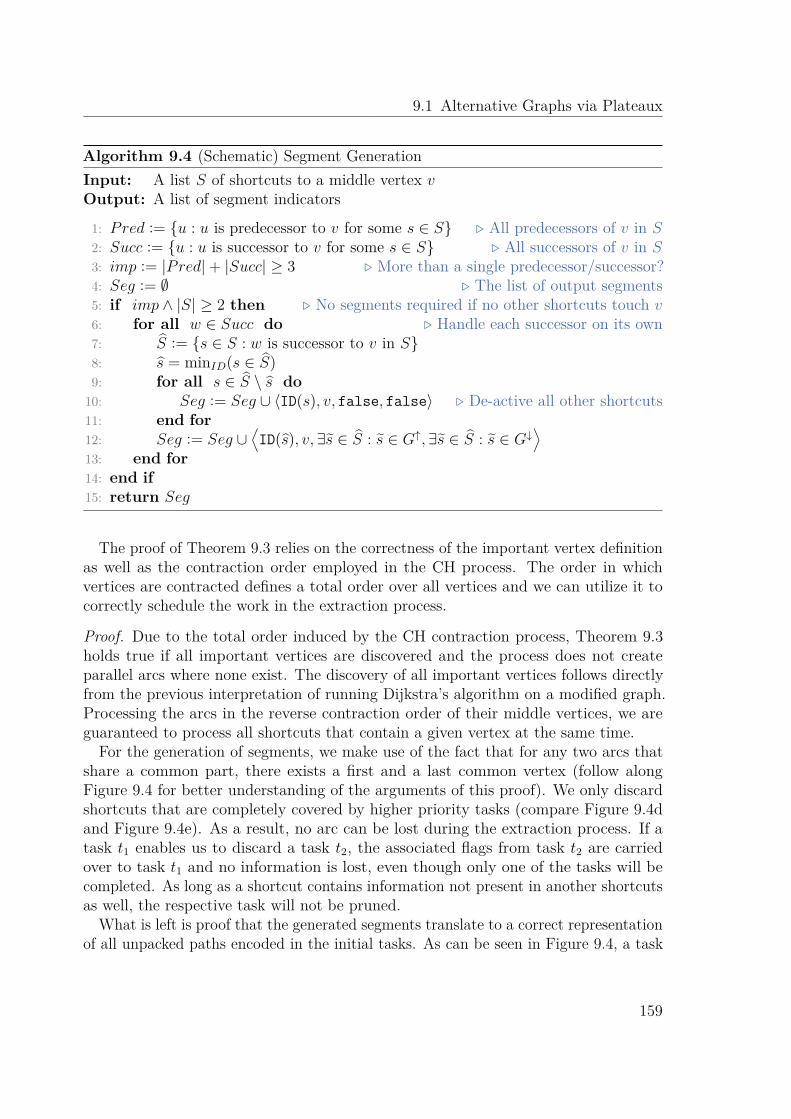
9.1 Alternative Graphs via Plateaux
Algorithm 9.4 (Schematic) Segment GenerationInput: A list S of shortcuts to a middle vertex vOutput: A list of segment indicators
1: Pred := {u : u is predecessor to v for some s ∈ S} � All predecessors of v in S2: Succ := {u : u is successor to v for some s ∈ S} � All successors of v in S3: imp := |Pred| + |Succ| ≥ 3 � More than a single predecessor/successor?4: Seg := ∅ � The list of output segments5: if imp ∧ |S| ≥ 2 then � No segments required if no other shortcuts touch v6: for all w ∈ Succ do � Handle each successor on its own7: S := {s ∈ S : w is successor to v in S}8: s = minID(s ∈ S)9: for all s ∈ S \ s do
10: Seg := Seg ∪ 〈ID(s), v, false, false〉 � De-active all other shortcuts11: end for12: Seg := Seg ∪
⟨ID(s), v, ∃s ∈ S : s ∈ G↑, ∃s ∈ S : s ∈ G↓
⟩13: end for14: end if15: return Seg
The proof of Theorem 9.3 relies on the correctness of the important vertex definitionas well as the contraction order employed in the CH process. The order in whichvertices are contracted defines a total order over all vertices and we can utilize it tocorrectly schedule the work in the extraction process.
Proof. Due to the total order induced by the CH contraction process, Theorem 9.3holds true if all important vertices are discovered and the process does not createparallel arcs where none exist. The discovery of all important vertices follows directlyfrom the previous interpretation of running Dijkstra’s algorithm on a modified graph.Processing the arcs in the reverse contraction order of their middle vertices, we areguaranteed to process all shortcuts that contain a given vertex at the same time.
For the generation of segments, we make use of the fact that for any two arcs thatshare a common part, there exists a first and a last common vertex (follow alongFigure 9.4 for better understanding of the arguments of this proof). We only discardshortcuts that are completely covered by higher priority tasks (compare Figure 9.4dand Figure 9.4e). As a result, no arc can be lost during the extraction process. If atask t1 enables us to discard a task t2, the associated flags from task t2 are carriedover to task t1 and no information is lost, even though only one of the tasks will becompleted. As long as a shortcut contains information not present in another shortcutsas well, the respective task will not be pruned.
What is left is proof that the generated segments translate to a correct representationof all unpacked paths encoded in the initial tasks. As can be seen in Figure 9.4, a task
159

9 A new Approach to Via-Alternatives
s1 t1
s2
s0
t2
t0v0
v1v2 v3
v4
(a) Graph
s0 t0 0 TF
v1s1 t1 1
TF
v0s2 t2 2
FT
v0
(b) Initial Tasks
Ft1 1t2 2
Tv1v1
v0v0 T
F
(c) Tasks generated at v0
v0 v1 2v2 TFFv1 1 Tv2 v0
s0 v1 0v2t0 0v3 v1t2 2v3 v1
T FT F
TF
v1 1v2 v0 TT(d) Tasks generated at v1
v2 v1 0v4 T Fv1 1v4 TTv2v1 0v4 T Tv2
(e) Tasks generated at v2
v0 T Tv0 F F
12
0 v2 T T1 v2 F F
0 v1 T T
2 v1 F F1 v1 FT
0 v3 T
2 v3 F
F
T
(f) Generated segments; each segment generated at the depicted vertex
Figure 9.4: Generation of segments and tasks on small problem – consisting ofthree shortcuts – chosen to exemplify the process. Lower numbers translate to higherpriorities (both for extraction order and for tasks). Grayed out tasks are temporarytasks – shown for illustration purposes – that are not actually created.
160

9.1 Alternative Graphs via Plateaux
may cause a deactivation segment which is followed by an activation segment later ondue to a completely different task; in the figure the task that extracts the shortcutwith ID two is deactivated at v0 by the task extracting the shortcut of ID one. Thecoverage in terms of the segments is handed over to the task with ID zero at v1 andthe task is finally activated again at v3. The argument for this process is simply basedon the first and last common vertex. When a task t is first deactivated at some vertexv, then v is the first common vertex with another task. These two tasks also have alast common vertex w. Either we create an active segment for task t at vertex w, or –in the case that another task of higher priority is present – transfer the coverage overto this higher priority task. In the case of the transfer, w acts as new first commonvertex between t and the new task and the last common vertex argument is postponedfor later on but remains valid3.
From the list of shortcuts and the segment indicators, we finally construct analternative graph. We scan the segment indicators associated with every shortcut andgenerate arcs for every active segment. Their length can be directly computed fromthe segment indicators. Every vertex that is part of an active segment indicator isselected as a vertex for the alternative graph.
9.1.5 Artificial ShortcutsA final piece of information is still missing from our algorithm. Until now, we onlyconsidered middle vertices and did nothing to handle the different origins and des-tinations of the initial shortcuts. We can easily integrate them transparently intothe full process, though. Our algorithms as presented so far consider all shortcuts inthe order of their middle vertices. To correctly integrate all arcs in this process andto process their origin and destination correctly, we simply wrap each arc into twoartificial shortcuts that have the origin and the destination as their respective middlevertices. As respective origin and destination of the artificial shortcuts we introducenew dummy vertices to the graph.
This extension comes cheap as we only require a simple scan over all arcs from thefirst phase. Due to the small CH search spaces the number of arcs is manageable. Tointegrate the artificial shortcuts into the unpacking process, we only need to appendinformation for the new vertices and their adjacent (artificial) shortcuts to the datathat guides the unpacking process. This augmentation presents the final step of ouralternative graph generation algorithm.
9.1.6 Additional ProcessingFinally, our algorithm performs a filtering step to keep the processing during theexecution as simple as possible. In this effort, we reduce the overhead required later in
3The order in which these local decisions are made does not matter for the correctness.
161

9 A new Approach to Via-Alternatives
u
v
(a) Arcu
v
u′
0
c(u, v)
(b) Packed Onceu
v
u′
v′
0
0c(u, v)
c(u, v)
(c) Packed Twice
Figure 9.5: Creation of artificial shortcuts to an arc (u, v). The additional verticesu′, v′ are connected to u, v via arcs of weight zero. The further process describes astraight forward contraction (see Algorithm 4.1) without any witness-searches.
an alternative route extraction.During the computation of the shortest-path distances, we prune all arcs from the
search space that offer a larger distance than desired4. Vertices with larger valuescannot influence the quality of our alternative graph in a positive way, as they wouldfail the admissibility criteria anyhow.
As a second optimization, we perform some additional post-processing that furtherhastens the alternative route extraction later on. Even though route extraction isnot part of HiDAR, we still assume the minimal quality criteria with respect to thedefinition of Abraham et al. (see Definition 5.3). We consider them by reducing thealternative graph to only contain plateaux of viable length in comparison to theirassociated detours.
For this filtering process, a localized view of the alternative graph is not enough.We tackle this problem with a DFS algorithm that keeps track of the current lengthtravelled along a plateau and the distance from the source; see Algorithm 9.5 andFigure 9.6 for reference.
The tree-like structure of the alternative graph, as long as we restrict it to the arcsfrom the forwards search, guarantees our DFS to always find correct values for thelength of our plateaux. The moment our algorithm discovers the end of a viable plateau,we track the arcs of the backward tree to the target. Along the way, we mark whichparts of the tree have to be remembered. During the backtracking steps of the DFS,we also mark the paths that lead to a plateau that has been deemed long enough.
When tracking the paths to the target, we could end up performing work quadraticin the number of vertices. We prevent this by marking the vertices appropriately, whichensures that we only touch every arc in the graph once.
4D (s, v) + D (v, t) ≥ (1 + ε) · D (s, t) .
162
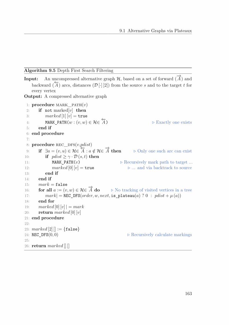
9.1 Alternative Graphs via Plateaux
Algorithm 9.5 Depth First Search Filtering
Input: An uncompressed alternative graph H, based on a set of forward (−→A ) andbackward (←−A ) arcs, distances (D [·] [2]) from the source s and to the target t forevery vertex
Output: A compressed alternative graph
1: procedure mark_path(v)2: if not marked[v] then3: marked [1] [v] = true4: MARK_PATH(w : (v, w) ∈ H∈ ←−
A) � Exactly one exists5: end if6: end procedure7:8: procedure rec_dfs(v,pdist)9: if ∃a = (v, u) ∈ H∈ ←−
A : a /∈ H∈ −→A then � Only one such arc can exist
10: if pdist ≥ γ · D (s, t) then11: MARK_PATH(v) � Recursively mark path to target ...12: marked [0] [v] = true � ... and via backtrack to source13: end if14: end if15: mark = false16: for all a := (v, w) ∈ H∈ −→
A do � No tracking of visited vertices in a tree17: mark| = REC_DFS(order, w, next, is_plateau(a) ? 0 : pdist + μ (a))18: end for19: marked [0] [v] | = mark20: return marked [0] [v]21: end procedure22:23: marked [2] [] := {false}24: REC_DFS(0, 0) � Recursively calculate markings25:26: return marked [] []
163

9 A new Approach to Via-Alternatives
st
(a) Input
st
(b) Forward DFS
st
(c) Backward Propagation
st
(d) Result
Figure 9.6: Sequence showing the development of the extracted alternative graphthrough the DFS and the marked backwards paths to the final alternative graph ofour algorithm.
9.2 Experimental Evaluation
For the evaluation of HiDAR, we take a look at the different phases in the algorithm,both in terms of their workload as well as their measured running time. Since HiDARis basically parameter-free and depends only on the used CH and the maximal delayaccepted for an alternative route, the performance evaluation can be presented in onlya few paragraphs. During the execution of our algorithm, we choose ε = 0.25 – thevalue limiting the maximal allowed bounded stretch – in accordance to the related[ADGW13] and [LS12].
Workload. Even though the theoretical justification for CH is not yet fully understood(compare Section 4.1), its practical use on road networks is without question. In practice,the search spaces of a CH behave very well and grow slow with respect to the Dijkstrarank. We can observe this behavior in Figure 9.7 for the size of the explored searchspaces as well. The pruning mechanism works surprisingly well, considering that wediscover tentative distances later than the usual CH query – remember that we need
164

9.2 Experimental Evaluation
to generate the search space in reverse contraction order for the following sweep. Theselected number of vertices for further processing remains very small. For the mostpart, the resulting graphs contain far less than a thousand vertices. We visualize thenumber of number of vertices and arcs in our output in Figure 9.9.
The workload during the processing of the different tasks, as well as the generatedsegments, grow stronger than the selected vertices. They behave very similar tothe search space, though. Luckily, the amount of vertices and arcs encoded withinthe shortcuts remains manageable for all distances (see Figure 9.8). The resultingalternative graphs grow rather large. The employed filtering method, however, reducesthe graphs to a very reasonable size. The size still exceeds what would be suitable topresent to a human. It remains small enough for further processing using expensivealgorithms for the extraction of alternative routes, though. The number of verticesand arcs to represent all plateaux as well as the possible paths is relatively low andstays far below a thousand, even for extremely long travels. For a typical journey, wewould expect roughly around a hundred vertices and arcs.
Running Time. The running time required for HiDAR is, at least for the longerjourneys, dominated by the extraction process that can end up processing close to70 000 different tasks (or arcs). In spite of the potentially high costs for the extractionprocess, the running time for HiDAR remains well within the limit for an interactiveapplication, not exceeding fifty milliseconds. All reasonable queries are well within tenmilliseconds. The pruning mechanism, while effective, only proves relevant to shortrange queries as the shortest-path query itself plays only a minor role in the total costof the algorithm. The high cost for the extraction process fully justifies the approach todirectly create the compact representation during the extraction process over a variantthat performs an additional parse of the extracted data.
Extracting a series of alternative routes from the small alternative graph is easy:The precomputed plateaux can be chosen and selected and the adjacent paths have tobe traced back to the current graph for overlap. This requires only a few hops, though.The required running times are irrelevant, even for a full exploration, in comparison tothe previous extraction overhead and are well within a single millisecond for all queries.
Quality. In terms of quality, our implementation directly compares to previous via-vertex approaches, while offering higher success rates, closing the gap to X-BDV. Incomparison to other via-vertex approaches for the success rates, we close the gap tothe far slower 3-REV by fifty percent, ninety-nine, and a hundred percent for the first,second, and third alternative route. The gaps to the upper bound in the form of thefull plateau method (X-BDV) are nearly identical. At the same time, our algorithmoffers nearly identical running times to 3-CHV and is up to five times as fast as 3-REV.We still loose out on some of the possible via-vertexs, though.
As can be seen in Figure 9.11, the alternative routes found by HiDAR offer very
165

9 A new Approach to Via-Alternatives
●●
●●
●●
●●
●
●
●
●
● ●
●
500
1000
1500
210 211 212 213 214 215 216 217 218 219 220 221 222 223 224
Cou
nt
Dijkstra Rank
● Search SpacePruned VerticesSelected Vertices
Figure 9.7: Workload of HiDAR in terms of vertices over different Dijkstra ranks.Even though just a heuristic, the pruning mechanism works well.
●
●●
●
●●
●
●
●
●
●●
●●
●
100
1000
1000
0
210 211 212 213 214 215 216 217 218 219 220 221 222 223 224
Cou
nt
Dijkstra Rank
● Forward TasksBackward TasksSegments
Figure 9.8: The number of tasks reflects the growing number of arcs representedin shortcuts. Our pruning and compaction mechanisms manage to keep the numberof generated segments small, though. The final graph contains even fewer arcs asmany of the generated segments are inactive.
166

9.3 Conclusion
●●
●●
●●
●●
●●
●●
●● ●
1010
010
00
210 211 212 213 214 215 216 217 218 219 220 221 222 223 224
Cou
nt
Dijkstra Rank
● VerticesArcsFiltered VerticesFiltered Arcs
Figure 9.9: Juxtaposition of the filtered and unfiltered alternative graphs createdby HiDAR. The result of our algorithm presents a manageable graph that can easilybe exploited for further considerations. The size of the output does not exceed athousand vertices.
slow stretch (ε). As a direct result, the values for local optimality (β) are also verygood. These high values come at the price of a large amount of limited sharing (α),though. As with most CH based techniques, we can see a drop-off in quality at Dijkstrarank 224. This drop-off affects the success rate, Dtot, as well as the number of firstalternatives we can find.
9.3 Conclusion
The HiDAR algorithm can be seen as a middle ground between the initial via-vertexapproach [ADGW13] and the calculation of alternative graphs in [BDGS11]. In contrastto the work discussed in [BDGS11], we present the – to the best of our knowledge –only algorithm that actually computes all paths that form the alternative graph ona speed-up technique at once. Even though Bader et al. focus on full graphs in theirparadigm, they only present methods based on single shortest-path computations.
While we follow the general idea of Abraham et al. [ADGW13] in what constitutesa viable alternative route, we manage to alleviate one of the major problems thatcomes with the calculation of a collection of paths: the high cost that is associatedwith making an informed choice during the path selection. We manage to perform allviability checks required over the course of a single run. As such we manage to staycompetitive for a well informed choice. In this, we allow for more sophisticated ways
167

9 A new Approach to Via-Alternatives
to select alternative routes. Our algorithm is able to evaluate all candidates in full andto report the best alternative route, instead of the first viable one.
168

9.3 Conclusion
Dijkstra Rank
Tim
e [m
s]0.
010.
11
10
21 22 23 24 25 26 27 28 29 210 211 212 213 214 215 216 217 218 219 220 221 222 223 224
SP−SearchExtractionPostproc.Total
(a) Without pruning
Dijkstra Rank
Tim
e [m
s]0.
010.
11
10
21 22 23 24 25 26 27 28 29 210 211 212 213 214 215 216 217 218 219 220 221 222 223 224
SP−SearchExtractionPostproc.Total
(b) With pruning
Figure 9.10: Running time of HiDAR and its different components over a variationof different Dijkstra ranks. Especially lower Dijkstra ranks benefit from the pruningmechanism.
169

9 A new Approach to Via-Alternatives
●
●
●
●● ●
●● ● ●
● ● ● ● ● ● ● ● ●● ●
●
● ●●
●
●
●
●
●
●
●
●
●●
●●
● ●
●●
●●
●
010
2030
4050
6070
8090
01
23
45
67
89
10
22 23 24 25 26 27 28 29 210 211 212 213 214 215 216 217 218 219 220 221 222 223 224
Dijkstra Rank
Para
met
er V
alue
● ●α β ε ε−base success #alt δtot
Figure 9.11: Development of the quality parameters, according to Definition 5.3,for HiDAR.
170

10 Chapter 10
Alternative Routes via SegmentExclusion
Vertex exclusion, the dual approach to the via-vertex paradigm, offers a linkfrom the via-vertex approach to the penalty method. We study an intermediateapproach, the exclusion of segments, for its potential and discuss some exten-sions. This unpublished work is a proof of concept implementation of my ownand uses the mechanisms of CRP-π. The presented concept does not offer thesame quality as CRP-π but reduces the workload. In addition, it could offera way to introduce penalization to Contraction Hierarchy (CH)-based routingengines. The evaluation on a CH is a topic of future work, though.
Although seemingly unconnected at first glance, the exclusion of vertices introducesa connection between the penalty method and via-vertex algorithms. The exclusionof a single vertex1 can be described as dual to the via-vertex paradigm. At the sametime, it is a special form of penalization. In fact, our implementation uses the samecode for penalization as CRP-π. The main difference is given in our approach ofdirectly choosing a very high penalty. This penalty has to be chosen high enough as toessentially block off the vertex while still keeping the graph connected to avoid specialcases. Due to this near infinite penalty associated with segment exclusion, we callour algorithm Customizeable Route Planning with Infinite Penalization (CRP-∞). Asalready stated, our implementation uses CRP-π and simply applies a very high penaltyfactor.
Basically, the concept addresses two shortcomings of the previous techniques atthe same time. The main problem in the via-vertex method consists of discoveringpotentially good candidates (c.f. Section 5.2.3). To find candidates, current methods[ADGW13] relax the search criteria, using a heuristic that depends on up to k parentvertices. While heuristic relaxation of the hierarchic properties can yield surprisinglygood results, knowing about all possible candidates is preferable. Especially in a
1Our implementation actually considers a series of vertices.
171

10 Alternative Routes via Segment Exclusion
production environment, a heuristic that depends on a CH order can produce unwantedinconsistencies. If a dependency between the ordering mechanism and the discovery ofcandidates exists, different preprocessing runs can offer different results.
While the penalty method is consistent in our implementation of CRP-π, the thepenalization is depending on the metric and can be hard to tune correctly. Some specialcases also require adaptive penalties. For example, if we consider a near optimal detourfor a sub-path, see Figure 10.1, we might need small penalties to find it. If we penalizethe full path too strongly, we can end up discovering a worse alternative instead. Inadvance, it cannot be known what constitutes a good penalization scheme to a path,though. In comparison, see Figure 10.2, exclusion can handle the same situation well.
Furthermore, we currently require a lot of cores to effectively lower the cost of asingle iteration. If we apply parallelism, it would be more reasonable to test multiplecandidates at the same time. However, the iterative process of the penalty methodprevents this.
By avoiding regions of the path instead of penalizing a full path, we can solve many ofthese problems: we can both test multiple candidates in parallel and can avoid findinggood penalization schemes. Furthermore, we avoid the difficult discovery of via-vertexs.Finally, the restriction to a local penalization might allow an implementation on a CHas well.
These benefits do not come without their own attached drawbacks, though. Thehighest cost to pay, when we exclude full segments from a path, can be in the form ofvery high bounded stretch. Our experiments show, however, that high stretch is barelya real concern.
Parametric Penalization. The exclusion of segments is not the only possible way topotentially handle penalization better. Another option would be to consider advancedpenalization schemes that combine multiple forms of penalization. We could, forexample, start the algorithm using low penalty values and increase the values overthe progress of the algorithm. As we have seen in Section 8.1 and the accompanyingexperiments, we currently require to keep the number of iterations low. The penaltyfactor itself has only little effect on the cost of an iteration. Advanced penalizationschemes might required to increase the number of iterations, resulting in slower runningtimes.
10.1 The Concept of Segment Exclusion
The discovery of segments to consider is straightforward: the initial computation of ashortest path provides all potential candidates. Since we always search for the shortestpath anyway, their discovery implies no additional computation overhead.
Even though a study of the dual to the via-vertex approach – excluding a singlevertex – would have been nice, we found it to be unreasonable. Although working well
172

10.1 The Concept of Segment Exclusion
ψ · D
�+ ε
1.2 · D
ψ · �
u
w
Figure 10.1: Illustration of the idea behind our consideration of segment exclusion.The discovery of the alternative between u and w highly depends on the form ofpenalization and has a good chance to be missed. In cases of a large value for ψ ,the path with the deviation between u and w could still end up more expensive thanthe second and longer alternative path. This is the case for ψ > 1.2·D−�−ε
D−�. Small
values for ψ require a longer time to discover the long path, though.
in many situations – for example when blocking access to an inner city highway –, itdoes not work in general. For the most part, the exclusion of a single vertex results ina local detour that offers only little variation in the route. Therefore, we decided touse an intermediate approach: instead of penalizing the full path or excluding a singlevertex, we consider a segment for exclusion. For our purpose, we define a segment as aconsecutive set of vertices on the shortest path2.
This intermediate solution can still offer multiple benefits over the via-vertex and thepenalization approach. In segment exclusion, we vary the metric in a very simple form,compared to advanced penalization schemes. To realize the exclusion of a segment, wecan choose a high additive or multiplicative penalty. Doing so, we essentially forbidthe usage of any blocked segment, as long as it is not required to maintain a connectedgraph. Therefore, we can even reuse our implementation of CRP-π.
2We explicitly chose vertices over arcs, as the exclusion of vertices prevents the discovery of veryshort detours.
173

10 Alternative Routes via Segment Exclusion
D
�+ ε
1.2 · D
�
u
w
e1
e2
e3
Figure 10.2: In contrast to Figure 10.1, the variations on what to exclude resultin the discovery of all reasonable alternative routes. Excluding e1, we discover theshorter alternative path of length D + ε. Excluding e{2,3} , we can only discover thelonger path of length 1.2D .
While the approach is very similar to the penalty method, it is in many wayspreferable. The most obvious reason is in the computational overhead. Whereas thecustomization of the full path requires a lot of cells to be considered, a small segmentis restricted to only a few of them.
In addition, there is no benefit in testing multiple increasing penalties. Vertices inthe segment are either not used or essential to the query (e.g. due to a bridge or aborder between countries). Blocking a segment a second time by applying even strongerpenalties does not change this result.
Furthermore, we can perform many independent queries in parallel.The iterative process of the penalization still offers some benefits. The application
of penalties to detours does not come as naturally for the blocking approach as it doesfor penalization.
Segment Selection. Using segments of consecutive vertices for exclusion offers aninteresting trade-off between the number of starting locations to consider and thediscovery of new routes. As formulated in Definition 5.4, the amount of allowed sharing
174

10.1 The Concept of Segment Exclusion
D
v 0.2D
w
Figure 10.3: Schematic illustration of sufficient blocking locations. Considering ablocked segment length of 0.1 · D (st) and an alternative to at least 0.2 · D (s, t) ,the locations marked by the dots are sufficient to find most reasonable alternativeroutes.
between an alternative route and the shortest path is limited. Typically, the researchcommunity considers a maximum of eighty percent of sharing between the two pathsas viable. This, however, requires the alternative path to deviate from the shortestpath for a segment (σ) with L (σ) ≥ 0.2D (s, t) .
While we might find a good alternative route at practically every vertex, the purenumber of possible starting locations prohibits an exhaustive test. Luckily, we canapproximate the result of such an exhaustive exploration in a reasonable way: Weconsider segments that overlap by a fixed amount of their length. We provide themotivation for this argument in Figure 10.3, under the assumption of the usuallyrequired difference between the shortest path3. If we consider blocking a segment σof length4 L (σ), we test every segment that starts at distances equal to a multipleof L(σ)2
αD(s,t) . For example, if we consider L (σ) = 0.1D (src, t) and α = 0.2 , we blockevery segment that starts at multiples 0.05D (s, t) . We refer to this method as a-prioridivision. For every possible deviation of length αD (s, t) , this guarantees full segment
3Typically, the sharing is limited to eighty percent [ADGW13] (α = 0.2).4L (σ) ≤ αD (s, t) .
175
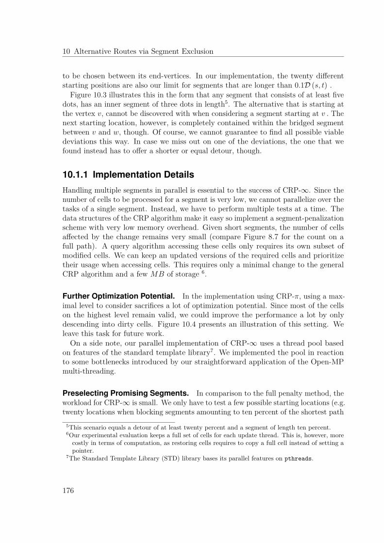
10 Alternative Routes via Segment Exclusion
to be chosen between its end-vertices. In our implementation, the twenty differentstarting positions are also our limit for segments that are longer than 0.1D (s, t) .
Figure 10.3 illustrates this in the form that any segment that consists of at least fivedots, has an inner segment of three dots in length5. The alternative that is starting atthe vertex v, cannot be discovered with when considering a segment starting at v . Thenext starting location, however, is completely contained within the bridged segmentbetween v and w, though. Of course, we cannot guarantee to find all possible viabledeviations this way. In case we miss out on one of the deviations, the one that wefound instead has to offer a shorter or equal detour, though.
10.1.1 Implementation Details
Handling multiple segments in parallel is essential to the success of CRP-∞. Since thenumber of cells to be processed for a segment is very low, we cannot parallelize over thetasks of a single segment. Instead, we have to perform multiple tests at a time. Thedata structures of the CRP algorithm make it easy so implement a segment-penalizationscheme with very low memory overhead. Given short segments, the number of cellsaffected by the change remains very small (compare Figure 8.7 for the count on afull path). A query algorithm accessing these cells only requires its own subset ofmodified cells. We can keep an updated versions of the required cells and prioritizetheir usage when accessing cells. This requires only a minimal change to the generalCRP algorithm and a few MB of storage 6.
Further Optimization Potential. In the implementation using CRP-π, using a max-imal level to consider sacrifices a lot of optimization potential. Since most of the cellson the highest level remain valid, we could improve the performance a lot by onlydescending into dirty cells. Figure 10.4 presents an illustration of this setting. Weleave this task for future work.
On a side note, our parallel implementation of CRP-∞ uses a thread pool basedon features of the standard template library7. We implemented the pool in reactionto some bottlenecks introduced by our straightforward application of the Open-MPmulti-threading.
Preselecting Promising Segments. In comparison to the full penalty method, theworkload for CRP-∞ is small. We only have to test a few possible starting locations (e.g.twenty locations when blocking segments amounting to ten percent of the shortest path
5This scenario equals a detour of at least twenty percent and a segment of length ten percent.6Our experimental evaluation keeps a full set of cells for each update thread. This is, however, more
costly in terms of computation, as restoring cells requires to copy a full cell instead of setting apointer.
7The Standard Template Library (STD) library bases its parallel features on pthreads.
176

10.1 The Concept of Segment Exclusion
t
s
Figure 10.4: Illustration of a fine grained query mechanism, only descending intodirty cells. The large cell on the right is used. Only in the updated part we use thelower level during the query.
in length). In addition, we can perform many of these tests in parallel. Nevertheless,we would like to to reduce unnecessary computations as much as possible.
Even if the number of threads does not matter, we cannot simply assign a singlethread to each of the tasks, as the memory bandwidth is limited. In a productionenvironment, the use of excessive parallelism is undesirable, as well.
Next to the previously discussed a-priori division, we can take a divide and conquerapproach as well. By recursively generating tasks, we can take the informationdiscovered in every step into account. If, for example, we find a very good detour for alarge part of the shortest path, it is very unlikely to find a different detour by blockinganother segment between its end-vertices.
Figure 10.5a illustrates this setting: if ε < δ, no segment exists for which we can findthe path using v2 . At the same time, the figure presents an example of a case in whichthe iterative approach of the classic penalization has a better chance of discoveringboth paths8.
Such a detour does not necessarily have to be an alternative to the full shortestpath, but rather to a significant portion of it. For the ranges next to the providedalternative, we continue in the normal recursive fashion.
The next case we consider is the discovery of essential vertices. If the penalized pathcontains some of the vertices that have been blocked off (see Figure 10.5c), we canassume that the respective vertices are essential to the shortest path. This definitionof essential is not as strict as the general concept of bridges in graphs, for which theremoval corresponds to the graph becoming disconnected. It is closely related, though.
8We can improve the exclusion method for this kind of setting, though. We describe how to do thisafter the current considerations.
177

10 Alternative Routes via Segment Exclusion
D
s
t
D+ε
D + δ
v1
v2
(a) Good Detour
s
t
Dd
j
(b) Local Detour
s
t
De0e1
(c) Essential Vertices
Figure 10.5: Illustration of some scenarios we can encounter during the recursivegeneration of tasks.
A vertex or arc is essential if its removal from the graph results in a significant detour;for example: the case of a bridge in a graph would result in a detour of infinite length.Due to our high penalization factors, a significant detour is equivalent to a penalizedarc to be part of the discovered path (e0 to e1 in Figure 10.5c). In case we discoversuch an essential range of vertices, we restrict the divide and conquer progress to omitthese vertices.
The final scenario we can encounter is the local detour (see Figure 10.5b). If wediscover a very high value for bounded stretch, we can handle it in the same way as wedo for the discovery of essential vertices.
Divide and Conquer Discovery. In our implementation, we assign regions to dif-ferent tasks. We describe the process for a segment length of 0.1D (s, t) and limitedsharing set to α = 0.2 . In the example of a single thread of execution, the initial regionwould be the full shortest path and we would consider a segment enclosing D(s,t)
2 inthe most balanced way9. After the task has been processed, we analyse the detour todecide how to generate further tasks. In case none of the formerly mentioned scenariosoccurs, we generate a task to the left that is in the middle of the region
[0, D(s,t)
2
]and
one for the region[D(s,t)
2 + 1, D (s, t)]
.In case of a good detour, we simply stop the recursion. In the other cases, we adjust
the regions to omit essential (or close to essential – compare the local detour) vertices.This method can be applied recursively until the respective regions get too small toplace a blocked segment of the desired length. By assuring an overlap of half a segment
9In this case balanced refers to the ranges to the left and to the right of the named location.
178

10.1 The Concept of Segment Exclusion
s0
e0
S0
s
t
(a) Level 0
s0
te1
e0
S0
s1
S1
s
(b) Level 1
t
S0s0
e0
s
(c) Level 2
Figure 10.6: Recursive levels during the task generation.
at the respective end vertices, we prevent our algorithm from blocking a segment morethan once.
We illustrate the process in Figure 10.6. The initial segment chosen is S0 inFigure 10.6a. The found detour crosses the blocked segment, influencing the choice ofthe recursive segments tested in Figure 10.6b, leaving a small gap between the respectiveend-vertices of the regions to be considered. After this initial first level, the rangecontaining S1 is considered too small for further recursion. Due to the different arcson the path, we can encounter the same situation for one part of the range containingS0 . In this example the effect results in a single range to be considered for recursioninstead of two ranges. The different positions of the respective S0 in Figures 10.6a and10.6c can result in subtle differences in the found alternative. These differences can beproblematic (c.f. Section 10.1.2) but can also be exploited (c.f. Section 10.1.3).
Heuristics. Instead of this divide-and-conquer approach, one could try to choosesegments heuristically based on many different influences. Local detours, the level ofdifferent vertices in the CRP data structures, or even vertex-reach could be considered.They are a topic of currently ongoing research, though.
Recursive Extension. The case presented in Figure 10.5a indicates a possibilityof further candidates if we recursively apply penalties to good detours. During thepreviously described divide and conquer approach, we remember which detours resultedin the pruning of sub-trees. For these detours, we perform additional steps after theinitial algorithm has finished. We start by first excluding the middle third of thealternative – the one that we remembered earlier – from the search. Afterwards, wesimply reinitialize the divide and conquer algorithm to continue at the previously
179

10 Alternative Routes via Segment Exclusion
pruned tree.
10.1.2 Potential Problems
As previously mentioned, one problem of this approach is that we can force thealternative route to start or end unreasonably. If we block off parts of the pathcompletely, we could end up producing very high stretch values. We can avoid most ofthese locally bad decisions with a simple trick: we only accept detours that start/endin a certain minimal distance to the blocked segment. To be exact, we postulate adistance between the segment and the deviation vertices of at least one percent ofD (s, t) . This reduces the occurrences of high stretch values to almost none. We onlyfound fifteen cases within our twenty-four thousand queries, for the most time offeringat most a fifty percent increase on a very short segment. Even though these problematicstretches are very undesirable, other techniques suffer from them as well. Abrahamet al. [ADGW13] report maximal stretch values of up to sixty-three percent increase(1-CHV, see Section 5.2.3), which is comparable to the fifty percent increase that weexperience in these rare cases.
In the cases for which we found high values for the bounded stretch, the values werevery close to the shortest path and described segments of very short length. We couldprobably corrected them by doing some local searches around the blocked segment.Due to the low rate of occurrence, we did not implement this, however.
10.1.3 Constructing an Alternative Graph
In the via-vertex paradigm, we compute a full graph in one query. In the setting ofCRP-π, we computed a growing number of paths and extracted viable segments fromthe set. Here, we take yet another approach. Unlike our previous approaches, CRP-∞computes many different paths in parallel.
The set of paths that we calculate can contain many similar ones, parts of whichmay be reasonable, parts of which might not be reasonable. We tried two differentmethods to construct a viable alternative graph. Our first idea to rank the differentpaths by a quality and select the best one for the graph did not work10. The reason forthis lies within the previously mentioned segments with bad stretch. Considering thepaths on their own, the rate in which we find locally high values for bounded stretchincreases, even though not to unreasonable levels. Still, we can combine the segmentsin a way that limits the number of bad paths that we encounter. We add all discoveredsegments into a large graph. On this graph, we apply a simple filter to then removesome unreasonable arcs. If two segments are parallel to each other, we discard oneof them, if they are too short on their own (less than the desired values for limited10We considered the length, the distance between the deviation vertices and the blocked segment, as
well as the stretch.
180
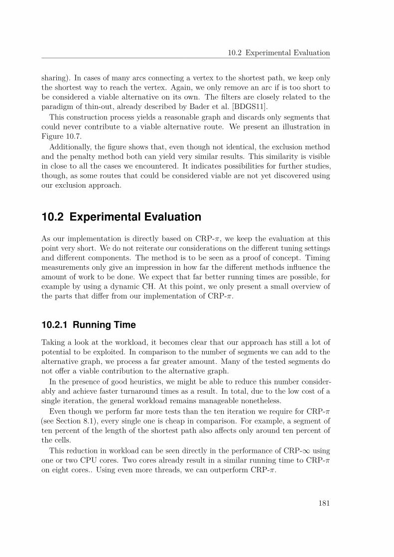
10.2 Experimental Evaluation
sharing). In cases of many arcs connecting a vertex to the shortest path, we keep onlythe shortest way to reach the vertex. Again, we only remove an arc if is too short tobe considered a viable alternative on its own. The filters are closely related to theparadigm of thin-out, already described by Bader et al. [BDGS11].
This construction process yields a reasonable graph and discards only segments thatcould never contribute to a viable alternative route. We present an illustration inFigure 10.7.
Additionally, the figure shows that, even though not identical, the exclusion methodand the penalty method both can yield very similar results. This similarity is visiblein close to all the cases we encountered. It indicates possibilities for further studies,though, as some routes that could be considered viable are not yet discovered usingour exclusion approach.
10.2 Experimental Evaluation
As our implementation is directly based on CRP-π, we keep the evaluation at thispoint very short. We do not reiterate our considerations on the different tuning settingsand different components. The method is to be seen as a proof of concept. Timingmeasurements only give an impression in how far the different methods influence theamount of work to be done. We expect that far better running times are possible, forexample by using a dynamic CH. At this point, we only present a small overview ofthe parts that differ from our implementation of CRP-π.
10.2.1 Running Time
Taking a look at the workload, it becomes clear that our approach has still a lot ofpotential to be exploited. In comparison to the number of segments we can add to thealternative graph, we process a far greater amount. Many of the tested segments donot offer a viable contribution to the alternative graph.
In the presence of good heuristics, we might be able to reduce this number consider-ably and achieve faster turnaround times as a result. In total, due to the low cost of asingle iteration, the general workload remains manageable nonetheless.
Even though we perform far more tests than the ten iteration we require for CRP-π(see Section 8.1), every single one is cheap in comparison. For example, a segment often percent of the length of the shortest path also affects only around ten percent ofthe cells.
This reduction in workload can be seen directly in the performance of CRP-∞ usingone or two CPU cores. Two cores already result in a similar running time to CRP-πon eight cores.. Using even more threads, we can outperform CRP-π.
181

10 Alternative Routes via Segment Exclusion
(a) Rank 21, Exclusion (b) Rank 21, Penalty
(c) Rank 17, Exclusion (d) Rank 17, Penalty
Figure 10.7: Examples of the generated graphs of our exclusion approach. Redarcs are only shown to indicate the discarded parts of the graph. For comparison,we show the same graphs as computed by CRP-π as well.
182

10.2 Experimental Evaluation
Dijkstra Rank
Tim
e [m
s]
0.1
110
100
21 22 23 24 25 26 27 28 29 210 211 212 213 214 215 216 217 218 219 220 221 222 223 224
T1T2T4T8T12
(a) A-Priori Division
Dijkstra Rank
Tim
e [m
s]
0.1
110
100
21 22 23 24 25 26 27 28 29 210 211 212 213 214 215 216 217 218 219 220 221 222 223 224
T1T2T4T8T12
(b) Divide and Conquer
Figure 10.8: Parallel execution of CRP-∞ on multiple cores. We only showexperiments for M2, as the memory on machine two has already proven fasterin the experiments for CRP-π. The segment length is chosen as ten percent ofD (s, t) .
183

10 Alternative Routes via Segment Exclusion
Dijkstra Rank
Slo
wdo
wn
11.
52
2.5
21 22 23 24 25 26 27 28 29 210 211 212 213 214 215 216 217 218 219 220 221 222 223 224
●
●
●
●
●
●
●
●
●
●
●
●●
●● ●
● ●●
●●
●●
●
● ● ●● ●
●● ● ●
● ●
●
● ●● ● ● ● ● ● ●
● ●●
● ●S5 S7 S10 S12 S15 S17 S20
Figure 10.9: Slowdown in comparison to the fastest run for different segmentsizes (SX specifies a segment of X
100 · D (s, t) in length.
Parallel Execution. Our measurements for the parallel execution of the algorithm,visualized in Figure 10.8, indicate that our algorithm is bound by the memory band-width, as long as we use more than four threads. Up to four threads, the parallelalgorithm scales well, which is to be expected for a set of independent tasks. Thiseffect is similar to the results that we experienced for the penalty method (CRP-π)and indicates potential for further improvements by reducing the memory footprint ofour application.
Segment Size When it comes to running time, it turns out that the actual segmentsize barely influences our algorithm. This is a result of the direct dependence betweenthe number of update tasks and the workload of a single task. In the end, both factorsbalance each other out. We visualize this effect in Figure 10.9, which shows only aslowdown of around forty percent between the slowest and the fastest setting. For thiscomparison, we ignore the effects of the short-range queries, as their running time isfast enough for all variants. In general, segment sizes result in faster queries.
Divide and Conquer vs. A-Priori Division When comparing Figure 10.8b toFigure 10.8a, we can see that the divide and conquer approach helps in speeding up thealgorithm. The information gained in the process can actually reduce the computationaloverhead. Still, the low number of unique routes we discover in comparison to the large
184

10.2 Experimental Evaluation
number of tested cases indicates that we could do even better with heuristics.Nevertheless, the divide and conquer approach is a step into the right direction.
The sequential performance is improved greatly in comparison to the a-priori division.Starting at four CPU cores, however, the two approaches break even.
10.2.2 Quality
When comparing our efforts for segment-exclusion to the general penalization (seeFigure 10.10), we can identify some interesting developments. Apparently, the qualityof the first chosen alternative for exclusion offers far greater values for local optimality(β) than we can see for CRP-π. This comes at the cost of limited sharing (α). Thebounded stretch (ε) remains lower than the values for CRP-π, indicating higher qualityfor the found detours. We can, however, see a severe drop-off in terms of number the ofalternatives and Dtot for long-range queries. Depending on the desired setting, blockingsegments can offer a viable choice, though. They are competitive in their quality forlow-range and mid-range queries. Especially in the combination with a dynamic CH,the method should be explored further.
Divide and Conquer. The decrease in computational cost we have seen comes at aminor decrease in quality.
Considering individual factors in our algorithm is difficult as all parameters influencethe algorithm in a major way. To test these influences, we performed a series ofexperiments varying the sequence size to be selected from {5, 7, 10, 12, 15, 17, 20}, usingfour cores and performing our recursive approach as well as a-priori division for taskgeneration.
While there is some minor variation, the number of segments we can add to thealternative graph remains close to identical for most Dijkstra ranks. Higher ranks aremore sensitive with respect to the number of alternative routes found. The variationcomes at the price of a larger number of decision arcs. Their count still remains withinthe acceptable limit of at most ten, though. The general success rate for the firstalternative route remains the same.
Segment Size In general, it seems to be possible to select a wide range of possiblesegment lengths, depending on the distance between the respective source and targetvertices. Most choices yield a very similar result in pure numbers, even though theactual paths differ. In our experiments, the union of multiple alternative graphs,computed with different segment sizes, yields better results than the graphs on theirown. Nevertheless, we propose a segment length of 0.1D (s, t) as a general setting thatworks well in practice.
Increasing the length past the chosen ten percent only shows little benefit.
185

10 Alternative Routes via Segment Exclusion
●
● ●
●●
● ●● ● ● ●
● ● ● ● ●● ●
● ●●
●
●
●●
●
●
●
●
●
●●
●
●
● ● ●
●● ●
●
●●
●● ●
010
2030
4050
6070
8090
01
23
45
67
89
10
21 22 23 24 25 26 27 28 29 210 211 212 213 214 215 216 217 218 219 220 221 222 223 224
Dijkstra Rank
Para
met
er V
alue
● ●α β ε ε−base success #alt δtot
(a) CRP-π
●
●
●●
● ●●
● ● ●●
● ● ● ● ● ●●
●● ●
●
●●
●
●●
●
●
●
●
●
● ● ●
●● ●
●
● ●
●● ●
010
2030
4050
6070
8090
01
23
45
67
89
10
21 22 23 24 25 26 27 28 29 210 211 212 213 214 215 216 217 218 219 220 221 222 223 224
Dijkstra Rank
Para
met
er V
alue
● ●α β ε ε−base success #alt δtot
(b) CRP-∞
Figure 10.10: Development of the quality parameters, according to Definition 5.3,for CRP-π and CRP-∞.
186

10.2 Experimental Evaluation
● ● ● ● ● ● ● ● ● ●●
●● ● ● ● ● ●
●● ●
●
● ●
●●
●
●
●
●
●
●
●
●
● ● ●● ● ●
●
●●
●●
●
01
23
45
67
89
10
010
2030
4050
6070
8090
100
21 22 23 24 25 26 27 28 29 210 211 212 213 214 215 216 217 218 219 220 221 222 223 224
Dijkstra Rank
Mea
sure
s
Suc
cess
Rat
e [%
]
●
●
totavgalts#dec. arcssuccess
(a) A-Priori Division
● ● ● ● ● ● ● ● ● ●●
●● ● ● ● ● ● ●
● ●
●
●●
●●
●
●
●
●
●
●
●
●
● ● ●● ● ●
●
● ●
●●
●
01
23
45
67
89
10
010
2030
4050
6070
8090
100
21 22 23 24 25 26 27 28 29 210 211 212 213 214 215 216 217 218 219 220 221 222 223 224
Dijkstra Rank
Mea
sure
s
Suc
cess
Rat
e [%
]
●
●
totavgalts#dec. arcssuccess
(b) Divide and Conquer
Figure 10.11: Juxtaposition of the quality of results from the divide and conqueras well as the a-priori division concepts. Our algorithm considers a segment sizeof ten percent of the shortest path in length.
187

10 Alternative Routes via Segment Exclusion
● ● ● ● ● ● ● ● ● ●●
●● ● ● ● ● ● ●
● ●
●
●●
●●
●
●
●
●
●
●
●
●
● ● ●●
● ●●
● ●
●
●
●
01
23
45
67
89
10
010
2030
4050
6070
8090
100
21 22 23 24 25 26 27 28 29 210 211 212 213 214 215 216 217 218 219 220 221 222 223 224
Dijkstra Rank
Mea
sure
s
Suc
cess
Rat
e [%
]
●
●
totavgalts#dec. arcssuccess
(a) Five Percent
● ● ● ● ● ● ● ● ● ●●
●● ● ●
● ● ● ●● ●
●
● ●
●●
●
●●
●
●
●
●
●
● ● ●
● ● ●
●
●●
●● ●
01
23
45
67
89
10
010
2030
4050
6070
8090
100
21 22 23 24 25 26 27 28 29 210 211 212 213 214 215 216 217 218 219 220 221 222 223 224
Dijkstra Rank
Mea
sure
s
Suc
cess
Rat
e [%
]
●
●
totavgalts#dec. arcssuccess
(b) Fifteen Percent
Figure 10.12: Quality comparison of additional segment sizes (A-Priori Division).
188

10.3 Conclusion
10.3 Conclusion
Excluding segments from the search provides a middle ground between the two majorparadigms considered in the computation of alternative routes, the via-vertex and thepenalty method. Finding potential points of application is straightforward, opposedto the difficult search for candidates in the via-vertex paradigm. The penalization isless complex than the one required for the penalty method (CRP-π). The restrictionto different parts of the shortest path allows for the parallel discovery of multiplecandidates, potentially even in a distributed setting. These benefits come at the priceof less guarantees with regard to the quality of the route. The only guarantee thatwe can possibly give is that the stretch along the found alternative will, at no point,exceed the factor of penalization. This factor depends on the length of the segment,though, and can be potentially very high. Even though this effect seems to occur onlyin a negligible number of cases and for far lower stretch values, possible additions tocompletely prevent it are required before such an approach can be used in a commercialsystem.
Also, while requiring less computational overhead than CRP-π, it would be desirableto operate sequentially by finding a good heuristic to select segment candidates insteadof recursively creating them. In even further additions, one could forgo the updateentirely and check the possibility of dirty regions which the search has to descend into,as would be the case with a dynamic CH. Since only a small set of them is affected,this should allow for a reasonable query time without the required update overhead.Even though our current implementation does not allow for a computation belowthe desired bound of a hundred milliseconds for all types of queries, the single-coreperformance is already very impressive. Using as much as four cores, we reach anaverage of around a hundred and fifty milliseconds, even for the longest long-rangequeries. For future research, the discovery of better heuristics could replace the divideand conquer approach. This could allow for an algorithm that provides high qualityalternative routes while operating within a hundred milliseconds for all queries.
In total, we have proven the exclusion of segments to be a viable method for alternativeroute computation. For good performance, heuristics to find reasonable locations haveto be explored. The expected problems in quality are nearly non-existent.
189


11Chapter 11
On a Hybrid NavigationScenario
Our final method for alternative routes originates in a hybrid routing scenariothat combines mobile navigation with powerful servers for computation. Thechapter is based on a fruitful collaboration on [DKLW12]. The implementation,which was done by me for the original publication, has been greatly extendedfor this chapter. Also, the analysis is a result of my own efforts. The initialidea of a corridor can be attributed to Daniel Delling and Renato Werneck.
The wide distribution of smart phones makes mobile navigation services omnipresent.Internet connectivity is available not only in the form of stationary Wireless LocalArea Networks(WLANs) but also over the phone network itself. Most techniques forfast shortest-path computation require powerful hardware to work efficiently. Someof them can be implemented on a mobile phone with limited compute capabilities(compare [GSSV12]), though.
A common approach to offering navigational services on a mobile device is todistribute the workload between a server and the device. In most scenarios, the phonetakes care of the rendering process as well as the voice assists. The computation of theshortest path takes place on a powerful compute server that only transfers the result tothe phone. By splitting the computation in such a way, the mobile device only needsto be able to render and display the route but not to compute it itself. As a result, thenavigation algorithm can be far more complex.
By focussing only on the displaying part, the driver may experience a potential lossof service in areas with bad or even no connectivity at all. Consider a situation inwhich a driver comes upon a complicated intersection offering a number of possiblechoices on how to continue. If the driver misses the desired turn, the navigation devicehas to offer a new path.
In case of a loss of connectivity, a potential driver would have no choice but to turnaround. If a u-turn should not be possible, he might even have to guess a way backto the proposed shortest path. In the presence of multiple viable paths from a source
191

11 On a Hybrid Navigation Scenario
to a target, the option to turn around might be unnecessarily bad in comparison toan updated path. When we take reaction times into account, it becomes even moreimportant that an updated route can be presented quickly. A quick response can endup saving the driver from a very long detour. As such, not only the complete lossof connectivity might influence the quality of service but also a slow mobile Internetconnection could suffice for a negative experience.
We present a method –initially published in [DKLW12] – that provides means ofhandling such situations quickly and without the requirement of communicating witha server. We approach this scenario by not only transferring a shortest path to themobile device but rather a meaningful Directed Acyclic Graph directed at the target.Within this DAG, which we call a corridor, the mobile device is able to correct somedriver-side errors on its own. This capability requires close to no additional computecapabilities on the device.
This chapter is separated into two parts. First, we discuss general ideas for corridors,independent of the way of computation. After this discussion, we focus on algorithmsto efficiently compute corridors using Contraction Hierarchies.
11.1 A General View on Corridors
We refer to a corridor in relation to a source vertex s and target vertex t in a graphG (V, A). Within this graph, a corridor is a DAG that is directed at the target in away that for every vertex v there exists a single next vertex to go to that is also withinthe corridor. Following these vertices results in a shortest path from v to t. Formally,we provide Definition 11.1.
Definition 11.1 (Corridor). Given a graph G (V, A), a source s, and target t: acorridor to s and t is a set of vertices Γ with s, t ∈ Γ that respects the shortest-pathdistances in G , i.e. DΓ (v, t) = DG (v, t) ∀v ∈ Γ . Furthermore, every vertex v in Γ isassigned a parent (p) vertex, such that D (v, t) = μ (v, p) + D (p, t) .
Some simple examples of valid corridors are the shortest path from a source s to atarget t, or even a full shortest-path tree, directed at t. The main goal of this chapteris to explore different options in between these two extremes.
The benefits of the corridor approach to navigation are twofold. First, the corridorprovides robustness in a scenario where the loss of connectivity poses a threat. Secondly,a corridor provides immediate updates to the driving direction in case of a missedturn/exit, due to the stored parent vertices. Using these vertices, a shortest pathcomputation translates to a simple traversal.
Even additional information, like the estimated arrival time, can be stored withevery vertex, if it should be required. This simplicity in the shortest-path computationpredestines corridors for fast computation of new routes on devices with low computa-tional power. This compute capability is limited tot he corridor, though. As a direct
192

11.2 Search Space Corridors
result of this limitation, we ask the question of how robust a corridor is against leavingit.
The property of robustness is difficult to grasp, as it is near impossible to describea typical traversal of a corridor. Of course, a full shortest-path tree is robust againstall possible kinds or errors. At the same time, the shortest path alone cannot be usedto correct for even a single deviation. It is unclear however, what the best choices inbetween might look like. For example, we expect far more errors in highly complicatedhighway ramp configurations or complex intersections than on general highway segmentsin which the directions request only to continue on the same road. The subjectiveimpression of complexity is hard to translate into an accurate measurement. Weprovide Definition 11.2 for the evaluation in the context of this thesis.
Definition 11.2 (Robustness). We define the robustness of a corridor Γ with respectto a type of driver. Any driver can be seen as the model of some form of randombehavior, not following the proposed route with some given probability. The robustnessof a corridor is defined in form of a success rate indicating the percentage of driversthat reach their destination without leaving the corridor. We refer to the robustness ofa corridor as � (Γ).
In the following Sections, we explore reasonable ways to compute possible corridors.
11.2 Search Space Corridors
The most obvious method for computing a corridor is to utilize the information alreadyprovided by a known speed-up technique. Pruning methods, for the most time, arenot able to reduce the information to the shortest path alone. The – in terms ofshortest-path computation – superfluous information might actually present a viableselection for corridors.
11.2.1 Goal Direction
To lessen both the computational and memory overhead involved with corridors, wecan prune parts of the shortest-path tree. The most obvious choice would be to notconsider the full shortest-path tree but rather restrict the search to all vertices thatcan reach the target within (1 + ε) · D (s, t) . In the case of driving directions, thisapproach considers a lot of unreasonable vertices for potential deviations; detours thatoriginate from failure to follow the given directions can be expected to stay withinsome vicinity of the shortest path. Considering both the source and the target, we canachieve better pruning by employing goal-direction techniques like ALT or ArcFlags.Both techniques offer reasonably low query times to be considered, we argue that theyare unreasonable nonetheless.
193

11 On a Hybrid Navigation Scenario
ALT-corridor. When we consider a complete run of Dijkstra’s algorithm, the shortest-path tree – or even a pruned one – provides information on vertices far beyond thedesired destination of a drive. The circular way in which the algorithm operates(compare Figure 3.1) results in a large amount of information on paths leading awayfrom the desired target. A way to circumvent this could be to perform a bi-directionalsearch and only to consider vertices v with D (s, v) + D (v, t) ≤ (1 + ε) · D (s, t) , whichwe can, for example, achieve using the ALT algorithm.
We can even execute some control over the technique and the number of verticesincluded by choosing different values of ε . Results in the context of the penalty method([PS13]) indicate a large associated overhead for this technique, though. The largeamount of required vertices brings us to the decision to not investigate this methodany further.
ArcFlags Corridor. An alternative method for a the calculation of a corridor wouldbe to consider ArcFlags as a pruning technique1. Searching from the target backwardsalong the flagged arcs to the source, we can keep all vertices v in the corridor that donot violate D (v, t) ≤ (1 + ε) · D (s, t) . In relation to the ALT-based version, we expecta less dense corridor than a ALT-based corridor at the cost of far lower robustness.The main reason for this loss in robustness is founded in some artefacts that are typicalfor the ArcFlags algorithm, fans and local queries. Figure 11.1 presents two exemplarycorridors and justifies our decision to also discard ArcFlags as a possible method.
These effects (compare Figure 11.1b) can be reduced by introducing multiple levelsof ArcFlags and using a bi-directional query. Doing so, we are still left with longsub-paths that offer no robustness. It is unclear, how the robustness along such apath might be increased in a natural way. A similar approach to the one we discuss inSection 11.8 could be possible, though.
11.2.2 Hierarchical Techniques
The other most frequently used methods are CH and CRP. We also considered thesearch spaces of both techniques. In terms of CH, the reasonable search space toconsider equals the graph computed by our own HiDAR algorithm. Similar to thesetting of the long paths already seen in Figure 11.1b, hierarchical techniques containmany long arcs. These long arcs lead to the same argument as we have already seenfor goal directed techniques; we give an example in Figure 11.2.
As a result, the search spaces of hierarchical techniques alone cannot be considereda viable choice for a reasonable corridor. They could offer a viable starting position,though, forming a reasonable base for one of the two techniques that we describe inthe next sections.
1We thank Dennis Schieferdecker for providing us with the ArcFlags for our graph.
194

11.3 Turn Corridors
(a) Local Area (b) Long Path
Figure 11.1: Graphical representation of two ArcFlags corridors. In a local area(cell), all flags are set to true. This prevents any pruning close to the target. Atthe end of a long path, ArcFlags suffer from a fan-like effect. Both problems can bealleviated (multi-level ArcFlags / bi-directional implementation – see Section 3.1).The technique does not provide promising solutions for all problematic parts, though.
11.3 Turn Corridors
Our first model considers the scenario which we mentioned a few times already: adriver might exhibit erroneous behavior. These errors could manifests themselves inwrong turns along the given directions. We directly translate these wrong turns intoour corridor definition and, accordingly, name this model a turn corridor (compareFigure 11.4a).
A turn corridor can be inductively described: initially we start with the shortestpath which forms a turn corridor of degree zero. Given a corridor of degree d, we cancalculate the next degree corridor by augmenting the degree d corridor with all verticesthat are directly connected to it. Finally, we compute the shortest-path hull of thevertices by including the shortest paths from all of these vertices to the target. Theformal description of a turn corridor is given in Definition 11.3.
Definition 11.3 (Turn Corridor). Given a source vertex s and a target t in a graphG (V, A), a turn corridor of degree zero is given by Γ0 := Πs,t . Inductively, we define
195

11 On a Hybrid Navigation Scenario
Figure 11.2: Exemplary representation of a corridor based on HiDAR. In thesame way as we experience when using CRP, shortcuts (depicted here without theirrespective underlying road geometry) result in long (sub)-paths without means forcorrecting erroneous behavior. The query depicted illustrates a shortest path ofDijkstra rank of two to the power of nineteen.
a turn corridor of degree k + 1 to a corridor of degree k via the deviation verticesΔ (Γk) := {v ∈ V : ∃a = (u, v) ∈ A ∧ u ∈ Γk} as: Γk+1 = Γk ∪ {u ∈ Πv,t : v ∈ Δ (Γk)} .
This inductive definition provides a natural way of managing the required robustnessin the trade-off with relation to corridor size. The calculation is simple as we do notrequire a multi-source shortest-path computation. Instead, we can simply traverse thecorridor and scan arcs to find the deviation vertices. Next, the inductive definition alsoprovides means to correct errors on the paths we have found in the previous iteration,treating every vertex within a corridor in the same way.
11.3.1 Theoretical DiscussionsTurning to highway dimension (h), we can show this version of corridors to be limited(non-trivially) in their size. As we explained in Section 4.1.5, highway dimensionpostulates a small (h) shortest-path cover for all shortest paths of a given length in alocal area. Under a few reasonable assumptions, we can show that the size of a turncorridor is limited by O (h · n0.75). While, of course, a size this large is still impracticalfor large graphs, the limit only specifies a (non-trivial) upper bound. Our experimentsshow that the actual size of a corridor does not increase as much as this limit suggests.
Theorem 11.1 (Turn Corridor Size). Let G (V, A) be an undirected graph with con-stant maximum degree δ (·)max, highway dimension h and assigned metric μ, μ (a) ∈Θ (1) ∀a ∈ A . Moreover, let D (s, t) ∈ O (
√n) ∀s, t ∈ V . Then, |Γ1 (s, t)| ≤ h · n0.75
holds.Assuming a constant upper bound for the metric is a strong assumption. It can be
justified, though, as we can explicitly split long arcs, if necessary.
196
11.4 Detour Corridors
Proof. Let c := Θ ( 4√
n) and by extension D (s, t) ∈ O (c2) . We consider two cases.
Case 1 (D (s, t) ∈ ω (c)): We partition the shortest path Πs,t into O (c) parts, each ofwhich is at most c in length. In each of the resulting parts P i, we can select a vertexvi. Consider the balls of size 2c and 4c around vi : Due to μ (a) ∈ Θ (1) , any deviationvertex is contained within the ball of size 2c around vi . The subpath optimality, theprinciple that guarantees the correctness of Dijkstras’ algorithm, states that the prefixof a shortest path is a shortest path itself. In our case, we can postulate an optimalpath of length 2c at the beginning of each shortest path to the target; due to highwaydimension, this path is covered by one of h vertices within the ball of size 4c . Evenif all of the O (c) deviation vertices were assigned a distinct shortest path to one ofthese h vertices, the total number of vertices would still be bounded by O (c2). Sinceno shortest path can be longer than the equivalent of turning around and followingthe original shortest path, the length of the shortest path from the covering verticesto the target is also bounded by O (c2). Given that our partition consists of O (c)parts, the total amount of vertices in a turn corridor of degree one is bounded byO (h · c3). See Figure 11.3 for an illustration.
Case 2 (D (s, t) ∈ O (c)): The limited maximum degree gives |Δ (Πs,t)| ∈ O (c) . As adirect result, due to D (s, t) ∈ O (c) and G being undirected, we get a bound of O (c2)for the size of Γ1 .
Especially the assumption of distinct paths overestimates the size of the corridor.We expect many of the paths to the target to actually share vertices. In addition, wecurrently do not know any way of integrating the interaction between neighbouringballs.
11.4 Detour Corridors
Another possibility to compute corridors is to consider the notion of a realizationperiod. This realization period describes the reaction time that a potential drivermight require after making an error. Focused on the situation, a driver might take acertain time δt to realize new instructions from the navigation device. To compensatefor this, it seems reasonable to consider every location that is reachable within thetime δt when starting somewhere along the shortest path. In accordance to this limiton the detour δt, we refer to this setting as a detour-corridor.
These locations, or vertices, can be computed in a straightforward manner withDijkstra’s algorithm (Algorithm 2.2). Instead of staring an instance at a source, wesimply start at all locations along the shortest path at once. We can achieve thisbehavior by initially adding all vertices of the shortest path into the priority queue
197

11 On a Hybrid Navigation Scenario
vi
(a) Path Division
2c
O (c2)
hi
vi4c
(b) Local Deviations
Figure 11.3: Illustration of the proof to Theorem 11.1.
with a distance value of zero. During the algorithm, we limit the relaxation to onlyconsider vertices that are within the bounds given by δt.
If the value for δt is reasonably small, the number of vertices within this tube aroundthe shortest path can be expected to be small as well. The method already requiresmore effort than the turn corridor, though.
These vertices, settled in the expansion algorithm, are the initial part of the corridor.To form a valid DAG directed at the target t, we have to compute the shortest-pathhull of the vertices and add all found paths to the corridor as well.
Recursive Extension. The corridor can be extended in a recursive manner. Theprocess does not come as naturally as for the turn corridors, though. A direct recursiondoes not seem appropriate as it would, for the most part, double the tube around theshortest path in its size. Instead, we propose to focus on the vertices that currentlyoffer no deviation possibilities. We limit the recursion to vertices that part of pathsthat leave the tube of size δt around the shortest path. These vertices are discoveredafter the extension phase and are identified by not having any neighbours within thecorridor besides their respective predecessors/successors. To reduce the additional cost,we also propose to reduce the allowable detour with every recursive extension. For ourexperiments, we use deltat
2r , for the recursion level r .Schematically, these vertices can be seen in Figure 11.4b in form of the two additional
paths.
Detour Corridor Properties. As with turn corridors, we can limit the size of detourcorridors. As long as we limit the detour time to δt ∈ Θ (1), the arguments given inthe proof of Theorem 11.1 can be applied to detour corridor size as well. The only
198

11.4 Detour Corridors
t
sv
(a) Turn
s
t
δt
(b) Detour
Figure 11.4: Schematics of detour and turn corridors.
difference between the two is that the number of deviation vertices to a vertex isnot limited by the maximum degree but rather by πδ2
t (which is within O (1), givenour prior assumptions). We can even lower this bound to πδ2
t +√
n2δt√n
≈ 2δt on average,assuming a density of one of the vertices over the plane.
11.4.1 Attached ComponentsBoth of the discussed methods have the tendency to generate attached components.No matter how exactly the component looks, these components add little in termsof alternative routes, as they are entered and exited via the same arc. Therefore,testing for both bounded stretch and local optimality cannot yield a positive result.We propose two methods to filter out these kinds of components.
Bridge-Filtering. Bridge-filtering is the stronger filtering method of the two; abridge in graph-theory is an arc that, if removed, splits the graph into two components.We employ the standard DFS-based algorithm to detect bridges in an (undirected)representation of the corridor. To avoid side effects regarding the source and the target,we add an additional arc between these two vertices to ensure that they are located ona circle. The bridge detection algorithm finds all arcs that are not part of a circle. Ina second step, we scan the graph and remove all vertices and arcs that can only bereached using such a bridge. We illustrate this method in Figure 11.5b.
Topological-Tree-Filtering. The bridge-filtering method removes all attached com-ponents. If we want to provide correct route requests for all possible turns up to acertain limit, this removal of components can be seen as an extreme choice. A less
199

11 On a Hybrid Navigation Scenario
s
t
(a) Corridor
s
t
(b) Bridge Filtering
s
t
(c) Top. Tree Filtering
Figure 11.5: Visualization of our methods for attached component filtering. Thegray arcs and vertices visualize the part that is filtered by the two methods. The redarcs in Figure 11.5a indicate the location of bridges.
aggressive technique would be to use a method based on a topological sort. Ourtopological-tree-filtering only removes attached trees, as illustrated in Figure 11.5c,starting at their leaves. Again, we prevent possible side-effects on s and t by adding anadditional arc between them in an undirected interpretation of the corridor. Afterwards,we perform a topological sort, to remove all vertices that are connected to the corridorby exactly a single arc.
Drawbacks of Filtering. Filtering reduces the amount of unnecessary informationat the cost of corridor robustness2. When considering turn cost, it is unlikely that wewould have to ask the driver to perform a u-turn in a local area. By removing theseattached components, we lose some knowledge as well. Especially the bridge-filteringmethod removes information on all attached circles. It would be possible, however,to implicitly remember u-turns using the topological-tree-filtering on a turn corridor.Comparing the maximal number of wrong turns allowed and the number of wrongturns taken, we can detect whether a vertex would normally be in the corridor. Ifthe number of wrong turns taken is lower than the number of wrong turns during thecalculation, we know that the vertex is part of an attached tree and can safely requesta u-turn.
2We define our notion of robustness in the next Section.
200
11.5 Robustness
11.5 Robustness
The decision whether a corridor is robust is hard to make as it is near impossible todescribe what we would expect in terms of erroneous behavior from a driver. Next tothe complexity of the respective intersections, the various drivers using a navigationdevice cannot be pressed into a simple model. We still chose to simulate a series ofdifferent potential drivers to evaluate the corridor methods for their robustness.
11.5.1 The Random Drive Concept
Our concept to test a corridor is based on the general notion of random walks [Pea05].In our interpretation of the random walk, we take a look at random drives in a plane,limiting the drive to a reasonable setting. For example we assume that a driver withina corridor does not to suddenly turn around in the middle of a road and heads into theopposite direction. As a direct result of this assumption, we can limit the randomnessto events that occur at intersections.
After an initial error, this assumption might be invalid. If the driver can perform au-turn on the current arc, he can return to the shortest path on its own. If the u-turnis not possible, our corridor provides the correct next vertex to travel to.
The moment the GPS detects a deviation from the initial route – ideally this shouldhappen prior to a driver realizing its mistake, even though it is the other way aroundfor the most time – our algorithm can instantly supply the driver with an updatedroute information and accompanying driving directions. This still holds true, if thedriver turns around in the middle of the road. Due to the driver only being able toreach two locations for which the correct driving directions are already known, we canargue that the driver will either have settled for the new and updated route informationor return to his or her original trajectory. In both cases, further random u-turns arenot to be expected.
For our experiments, we tested a range of drivers, each of which is described in oneof the following paragraphs. At this point, we present a selection of the tested drivers.Further studies can be found in Appendix E.
The Adjusted RD Driver. We describe an adjusted deviation driver, or aRD, usingtwo probabilities p and p′ > p; p defines the probability of an initial wrong turn. Theadditional parameter p′ describes the probability of taking another wrong turn afteran initial mistake. This heightened probability of a wrong turn emulates a potentialpanic-driven reaction of a driver after discovering the initial mistake. After followingthe (updated) driving directions again, the driver switches back to the initial probabilityp . In our experiments, we use p′ = 2p .
201

11 On a Hybrid Navigation Scenario
Complexity Driver. We do not expect a uniform probability of taking a wrong turn.For example, as long as we continue on a road, we would not expect a driver to randomlymake a left turn. To account for this, we study the complexity-driven random deviationdriver (cRD). It is described in a single parameter p, which gives the probability of awrong turn. We scale this probability by |∠(u,v,w)−180|·k
90·2 p with k specifying the numberof potential wrong directions to travel in (except for u-turns).
Angular Resistance Driver. Bot previous drivers use wrong turns as their methodof deviation. While every deviation is initiated by a wrong turn, only considering turnswould result in a bias towards turn corridors. Similar to the model of corridors thatallow for a certain time of error, we model a driver based on an error period. Theangular resistance driver (AR) is parameterized by an error probability p and a timebudget t . Extending the cRD, we analyze the path for the angle present in the currentturn descriptions. An error occurs at v with probability |∠(u,v,w)−180|·k
90·2 p (compare cRD).After such an initial error, we switch to a deviation mode for a travel time of t. Whenthe driver’s state is in this deviation mode, rather than following the driving directionsspecified by the corridor, the driver automatically follows the path of least resistance.To be exact, we calculate the angle between the previously taken road segment andthe potential candidates. Among all candidates, we choose the one which is closest tocontinuing straight; in other words, for a road segment u, v we choose w to minimize∠(u, v, w) − 180 .
None of the presented drivers can be described as a very realistic model. Nevertheless,the tested drivers give a general idea of the entire concept and show the viability ofcorridors. A random wrong turn along a path seems rather unlikely. For a better model,we could even try to improve the corridor calculation to consider difficult intersectionsinstead of all intersections. This would allow for smaller corridors that are directed atcorrecting only a specific kind of mistake. We would require some information on thedifficulty of different intersections, though. An angular analysis as done for the AR orcRD could provide a starting point.
Corridor Robustness We evaluate a corridor by simulating a series of randomdrives for a given source and target pair. If the driver reaches an intersection that isnot within the corridor, we count the try as a failure, otherwise as a success. The onlyexception from this rule is the budgeted driving period of the angular resistance driver;here we check the inclusion property at the end of the driving period. The success rateof a corridor gives an intuition on how well the corridor can handle different rates oferrors.
202

11.5 Robustness
11.5.2 Evaluation
Before we consider the time necessary to compute one of our corridor models, we focuson their general properties. We evaluate them for both their size and the achievablesuccess rates in relation to the previously introduced random drivers. Following theextensive evaluation, we discuss an efficient implementation.
General Properties. In a hybrid scenario, we require a maximum quality of serviceat minimal expense. The expense is divided into two factors: the number of vertices inthe corridor and the time we have to invest in the computation. The latter is subjectto factors considered in the upcoming sections. At this point, we focus on the former.In the appendix, we present Figure E.5 and Figure E.6, to visualize the growth of therespective corridor models. In general, the detour corridor offers a lot of informationvery close to the shortest path and no robustness on longer alternative segments. Theturn model, on the other hand, offers the natural recursive extension and in extensionrobustness along most of the contained paths.
Judging purely by the visual representation (compare Figure 11.6), the recursivevariant of the detour corridor (Figure 11.6b) seems the most robust. In our experiments,we see the merits of both the turn variant as well as the recursive detour variant. Ingeneral, a high degree of robustness comes at the cost of a high number of verticeswithin the corridor – potentially too high for practical purposes.
We visualize the size of different corridor methods in Figure 11.7. Already relativelyshort random detours result in rather large corridors. A detour corridor for a tensecond detour (δt = 100) is comparable in its size to a turn corridor of degree three.Figure 11.6 indicates the turn corridor to be better suited to our cause, though. Ratherlong detours – i.e. longer than ten seconds – seem to generate corridors that are toolarge.
The corridors consist of, in comparison to the theoretical bound, far fewer vertices.Perhaps the most obvious reason behind this behavior is given in the low number ofdistinct reasonable paths between any given source and target. As a result, we expecta corridor to direct a driver directly back to the initial shortest path in the most cases.
As our model does not support turn penalties, one could offer criticism that the highnumber of expected u-turns effectively reduces the corridor to the shortest path andthe directly connected deviation vertices. To counter this argument, we provide thesame information for the arc-expanded version of the graph, a version in which u-turnsare penalized by a hundred seconds. We give a juxtaposition of corridors sizes for bothversions in Figure 11.8. While the switched setting does increase the corridor growth,the size remains manageable.
While the general size of the corridor gets far larger in the arc-expanded version ofthe graph, the relative growth between a corridor of degree i and one of degree i + 1remains at a relative factor of about two. This indicates that our methods do notbenefit in an unfair way from using the standard graph model over the arc-expanded
203

11 On a Hybrid Navigation Scenario
(a) δt = 100 (b) δt = 100, recursion depth: 3
(c) Two turns (d) Four turns
Figure 11.6: Juxtaposition of a detour corridor, a recursive detour corridor, andtwo different turn corridors on a short range query (Dijkstra rank 214 .
204

11.5 Robustness
●●
●●
●●
●●
●●
●●
●●
●
●
●
●
●
●●
●●
●●
●●
●●
●
Dijkstra Rank
Cor
ridor
Siz
e10
010
0010
000
210 211 212 213 214 215 216 217 218 219 220 221 222 223 224
●
●
1−turn3−turnδt= 100δt= 200δt= 100, R=3δt= 200, R=3
Figure 11.7: Corridor size in relation to Dijkstra rank for various corridor methods.δt/10 specifies the allowed detour in seconds and R the recursion level for the detourcorridor.
one. In addition, the methods that we are introducing in the upcoming sections performwell enough to handle even the arc-expanded graph fast enough for interactive settings,remaining within a hundred milliseconds for a six-turn corridor.
Success Rate. The different driver models favour different types of corridor models.The figures 11.9-11.12 illustrate the different corridor models and the experiencedsuccess rates. In every random drive we performed, we limited the time spent on thedrive to at most two times the length of the shortest path. Whenever a driver did notleave the corridor within this time-frame, the resulting drive is considered a success.
The detour corridors for ten and twenty seconds of allowed deviation (δt ∈ {100, 200})only show disappointing success rates. A single exception is the cRD driver who isexpected to take far less wrong turns than the other models and favours errors alongthe dense parts of the graph. In these sections, we expect far shorter arcs and as aresult a good coverage in the detour model. For lesser error probabilities, the successrates gradually improve, though.
The recursive variant of the detour corridor – both plots show a recursion depthof three – increases the chances of staying within the corridor. All success rates forboth the turn-by-turn driver models as well as the AR variants of the drivers stayrather poor, though. We can increase the recursive properties of the approach by not
205

11 On a Hybrid Navigation Scenario
● ● ● ● ● ● ● ● ● ● ● ● ● ● ●
●●
● ●●
●● ●
● ●●
●
●●
●
10
210 211 212 213 214 215 216 217 218 219 220 221 222 223 224
Rel
ativ
e S
ize
Dijkstra Rank
●
●
1−turn2−turn3−turn
4−turn5−turn6−turn
(a) Standard Graph Model (Graph 1)
● ● ● ● ● ● ● ● ● ● ● ● ● ● ● ●
● ● ● ● ● ●● ● ● ● ● ● ●
● ● ●
1010
0
210 211 212 213 214 215 216 217 218 219 220 221 222 223 224
Rel
ativ
e S
ize
Dijkstra Rank
●
●
1−turn2−turn3−turn
4−turn5−turn6−turn
(b) Arc-Expanded Graph Model (Graph G1e)
Figure 11.8: Corridor size (turn model) measured as a relative factor to theshortest path.
206

11.5 Robustness
Dijkstra Rank
Suc
cess
Rat
e [%
]
020
4060
8010
0
210 211 212 213 214 215 216 217 218 219 220 221 222 223 224
● ●●
● ●
●●
●●
●●
●● ●
●
● aRD cRD AR50 AR100
(a) δt = 100
Dijkstra Rank
Suc
cess
Rat
e [%
]
020
4060
8010
0
210 211 212 213 214 215 216 217 218 219 220 221 222 223 224
● ●● ● ●
●● ●
●●
● ●
●
●
●
● aRD cRD AR50 AR100
(b) δt = 200
Figure 11.9: Success rate in relation to the length of the shortest path for a detourcorridor; error probability set to ten.
207

11 On a Hybrid Navigation Scenario
reducing the size of δt in every recursion. This change results in far higher vertexcounts, though.
As to be expected, the turn model excels for the turn-based driver models. Theclose relation between the corridor model and the driver almost guarantees this. Wedo require some turns for the method to work, though. A three-turn corridor alreadyexhibits quite favorable success rates for most of the driver types. Only the AR50 andAR100 drivers provide an exception to this. The long reaction times of five and tenseconds respectively can be seen as unrealistic, though. A AR10 driver performs verywell (not shown), although a reaction time of one second should be equivalent to asingle turn anyhow.
Turning to rather extreme parameters (six turns and fifty seconds of random deviationc.f. Figure 11.12), we can see that corridors can handle even the most unrealisticscenarios rather well; the turn model outperforms the detour model (without recursion),except for very long routes in combination with the AR50 and AR100 driver.
Based on our experiments, we deem the turn model to be the most promising one.While the turn model performs perfectly for the turn-by-turn drivers, it even providesa good quality for the detour based drivers (AR model).
The detour models (both recursive and non-recursive) perform slightly better onthe detour-based drivers than the turn model, which is to be expected. For someparameter choices, however, the turn model of a corridor can already outperform thedetour model even for those drivers. The turn-by-turn drivers perform significantlyworse in the detour model. At the cost of a high increase of vertices, we can switchthis around by including all vertices that are connected to a road that is reachablewithin δt . We can, however, hardly justify this increase in vertices as the turn modelalready performs very well.
The computational methods of both variants are closely related and we invite thereader to make their own selection of models and parameters that best fit the desiredpurpose.
11.6 Attached Component Filtering
In the following sections, we present an experimental evaluation that shows the effectsof our filtering methods for attached components.
11.6.1 Corridor Size Reduction
The reduction of corridor size severely depends on the region that the path is locatedin. For example in cities, we can barely see any effect. The reason for this is the graphdensity. For longer range queries, the fact that a highway exit and highway entry aretwo distinct arcs prevents us from detecting them in our filters. Nevertheless, we can
208

11.6 Attached Component Filtering
Dijkstra Rank
Suc
cess
Rat
e [%
]
020
4060
8010
0
210 211 212 213 214 215 216 217 218 219 220 221 222 223 224
● ●●
● ●
●●
●●
●
●●
●●
●
● aRD cRD AR50 AR100
(a) δt = 100
Dijkstra Rank
Suc
cess
Rat
e [%
]
020
4060
8010
0
210 211 212 213 214 215 216 217 218 219 220 221 222 223 224
●● ● ●
●●
● ●
●●
●
●●
●
●
● aRD cRD AR50 AR100
(b) δt = 200
Figure 11.10: Success rate in relation to the length of the shortest path for arecursive detour corridor (depth of three); error probability set to ten.
209

11 On a Hybrid Navigation Scenario
Dijkstra Rank
Suc
cess
Rat
e [%
]
020
4060
8010
0
210 211 212 213 214 215 216 217 218 219 220 221 222 223 224
●
●
●
●
●
●●
●●
● ●● ● ● ●
● aRD cRD AR50 AR100
(a) One turn
Dijkstra Rank
Suc
cess
Rat
e [%
]
020
4060
8010
0
210 211 212 213 214 215 216 217 218 219 220 221 222 223 224
● ● ● ● ● ● ● ●●
●●
●
●
●
●
● aRD cRD AR50 AR100
(b) Three turns
Figure 11.11: Success rate in relation to the length of the shortest path for a turncorridor; error probability set to ten percent.
210

11.6 Attached Component Filtering
Dijkstra Rank
Suc
cess
Rat
e [%
]
020
4060
8010
0
210 211 212 213 214 215 216 217 218 219 220 221 222 223 224
●●
● ● ●●
● ● ● ●● ● ●
●
●
● aRD cRD AR50 AR100
(a) Detour corridor; δt = 500
Dijkstra Rank
Suc
cess
Rat
e [%
]
020
4060
8010
0
210 211 212 213 214 215 216 217 218 219 220 221 222 223 224
● ● ● ● ● ● ● ● ● ● ● ● ● ● ●
● aRD cRD AR50 AR100
(b) Turn corridor; six turns
Figure 11.12: Success rate in relation to the length of the shortest path for adetour corridor; error probability set to ten percent.
211
11 On a Hybrid Navigation Scenario
see a large reduction of vertices, when we apply either one of our filtering methods.We visualize the results in Figure 11.13 for both methods.
If we only desire the calculation of an alternative graph, further filtering couldtarget deviations that only offer little variation or very high stretch. Both kinds ofdeviation cannot be detected using our implemented filtering methods, though. Wepresent an overview of our filtering results in Figure 11.14 and Figure 11.15. The turncorridors can be reduced to about three-quarters of their unfiltered size. For a largernumber of turns, both the general reduction and the benefit of using bridge-filteringover topological-tree-filtering increase. As expected, the detour model holds a lot moreunwanted information. This results in a far greater reduction rate when we applyeither one of our filtering methods. The differences between bridge-filtering, which canachieve a reduction of forty percent, and topological-tree-filtering, which only reachesaround thirty percent, are far greater in the detour model. This further confirms thatlong detours in rural areas often contribute little to the alternative graph.
11.6.2 Robustness
The large reduction in size comes along with a reduced robustness as well. Unless wecan get hold of actual data that indicates where wrong turns happen, it is hard to arguehow to reduce a corridor in size. For example, we would expect a bridge-filtering to befully reasonable close to a turn that most likely will never happen. If a mistake werecommon at the given intersection, however, we would potentially only want to filterusing the topological-tree removal. Since both techniques remove a lot of the u-turninformation along a path, the success rates drop significantly, as shown in Figure 11.16,when compared to Figure 11.11 and Figure 11.9.
The filtering has its own justification, when considering corridors as a method for thecomputation of alternative graphs, though. Attached components cannot contribute toan alternative path in a reasonable way. Depending on the cost of the alternative routeextraction mechanism, applying a filter beforehand to reduce the workload can bebeneficial. Especially as our filtering methods both offer linear asymptotic guarantees.
11.7 Corridor Computation
For our considerations about an efficient implementation, we focus on the turn corridormodel. The ideas and methods that we develop in the following paragraphs can beapplied to the detour paradigm in the same way, though.
11.7.1 Conceptual Approaches
Computing turn corridors, especially if we consider their potential size, seems like adifficult task at first. The upper bound on their size, however, is rather large and we
212

11.7 Corridor Computation10
2030
40
21 22 23 24 25 26 27 28 29 210 211 212 213 214 215 216 217 218 219 220 221 222 223 224
Dijkstra Rank
Rem
oved
Ver
tices
[%]
●●
●● ● ● ● ● ●
● ●● ●
●● ● ●
● ●●
●
●●
●
● ● ● ● ●● ● ● ● ● ● ● ● ● ● ● ● ● ● ●
●
●●
●
● ●1−turn−TTF1−turn−BF
3−turn−TTF3−turn−BF
6−turn−TTF6−turn−BF
(a) Turn Corridors
1020
3040
21 22 23 24 25 26 27 28 29 210 211 212 213 214 215 216 217 218 219 220 221 222 223 224
Dijkstra Rank
Rem
oved
Ver
tices
[%]
●
●
●● ● ●
●●
●● ● ● ● ● ● ● ●
●●
●●
●
●● ●
●● ● ● ● ● ● ● ● ● ● ● ● ●
●
●
●
δt=100−R0−TTFδt=100−R0−BFδt=200−R0−TTFδt=200−R0−BFδt=200−R3−TTFδt=200−R3−BF
(b) Detour Corridors
Figure 11.13: Reduction of corridor size for a selection of corridor types(TTF=Topological-Tree-Filtering, BF=Bridge-Filtering). The detour corridor isspecified with respect to the allowed detour (δt/10 s and the recursion depth (R).
213

11 On a Hybrid Navigation Scenario
(a) Unfiltered
(b) Topological-Tree-Filtering (c) Bridge-Filtering
Figure 11.14: Visualization of our filtering methods. The example shows a fiveturn corridor on a Query of Dijkstra rank two to the power of nine.
214

11.7 Corridor Computation
(a) Unfiltered
(b) Topological-Tree-Filtering
(c) Bridge-Filtering
Figure 11.15: Visualization of our filtering methods. The example shows a detourcorridor of recursion level three with a initial detour of 20 seconds (δt = 200). Theused search is a query of Dijkstra rank two to the power of thirteen. 215

11 On a Hybrid Navigation Scenario
Dijkstra Rank
Suc
cess
Rat
e [%
]
020
4060
8010
0
210 211 212 213 214 215 216 217 218 219 220 221 222 223 224
●
●●
●
● ●● ●
●● ● ● ● ● ●
● aRD cRD AR50 AR100
(a) Three turn corridor
Dijkstra Rank
Suc
cess
Rat
e [%
]
020
4060
8010
0
210 211 212 213 214 215 216 217 218 219 220 221 222 223 224
●● ● ● ●
● ● ● ●● ● ●
●● ●
● aRD cRD AR50 AR100
(b) Detour corridor (δt = 200, three recursions)
Figure 11.16: Success Rates on a bridge-filtered corridor. The topological-tree-filtering method yields very similar results.
216

11.7 Corridor Computation
Algorithm 11.1 Simplistic Turn Corridor ComputationInput: A corridor Γof degree d to a target tOutput: A corridor of degree d + 1
1: D := {v ∈ V |∃a = (u, v) ∈ A, v /∈ Γ, u ∈ Γ}2: for all v ∈ D do3: Γ = Γ ∪ Πv,t
4: end for5: return Γ
have already seen that corridors contains only a fraction of the theoretically possiblevertices. A main reason for this is the limited number of alternative routes we can findeven with techniques like X-BDV, as – for the most part – the directions guide thedriver back to the initial shortest path.
For the computation of a turn corridor, we first present a preliminary algorithm (seeAlgorithm 11.1) that describes the general concept of our approach.
Though very simple in principle, the straightforward implementation exhibits a lot ofoptimization potential that we can exploit for an efficient algorithm for turn corridors.The expected form of a turn corridor exhibits some optimization potential. For themost part, we expect a small set of different shortest paths to the target and very shortdetours along these paths. So, let us first take a step back and examine a turn corridoralgorithm based on Dijkstra’s algorithm:
Dijkstra-based Corridor. To compute a turn corridor with Dijkstra’s algorithm, weinstantiate an implementation of the Algorithm searching backwards from the target,searching for the source s. As depicted in Algorithm 11.2, the further progress extendsthis potentially incomplete shortest-path tree whenever it should become necessary.
Computing the deviation vertices is straightforward. We traverse all vertices thathave just been added to the corridor Γ (initially this set is comprised of the shortestpath itself) and their adjacent arcs. All vertices that can be reached from one of thevertices of the last iteration and have not been added to the corridor are stored on astack for further processing3.
For every such vertex v, we need to find the shortest path to the target. To do so,we check whether v has already been settled by our instance of Dijkstra’s algorithm. Ifthis is not the case, we first continue the initial instances of Dijkstras’ algorithm untilwe settle v. Afterwards, we track the parent pointers until we reach the first vertexlocated within the corridor. By adding all the traversed vertices to the corridor, wecompute the shortest-path hull of Γ ∪ {v} .
The set of vertices extracted in this way forms a valid corridor which directly follows3The order we use here is not relevant for the correctness and ignored in Algorithm 11.2. It offers
better locality, though.
217

11 On a Hybrid Navigation Scenario
Algorithm 11.2 Dijkstra-based Turn Corridor ComputationInput: A corridor Γof degree d to a target t in the form of a tree pointing at t, a
partially completed instance of Dijkstra’s algorithmOutput: A corridor of degree d + 1 in the same form
1: p [·] =⊥ � Parent pointers to every vertex2: D := {v ∈ V | ∃ a = (u, v) ∈ A, v /∈ Γ, u ∈ Γ}3: for all v ∈ D do4: while not settled[v] do5: step_dijkstra()6: end while7: for all (u, w) ∈ Πv,t, u /∈ Γ do8: Γ = Γ ∪ u9: p [u] = w
10: end for11: end for12: return Γ
from the correctness of Dijkstra’s algorithm. Every vertex v in the corridor is onlyadded once and examined at most δ (v) times, each arc at most looked at from both itsorigin and destination. As a result, the running time of Dijkstras’ algorithm dominatesthe execution of the corridor method.
For small distances between s and t, this algorithm might even perform well enough,losing its practicality on larger instances, though, as the running time of Dijkstra’salgorithm gets longer. Nevertheless, we utilize it as a comparison algorithm and referto this simple version as dijkC.
The most obvious approach at this point is to turn to speed-up techniques. A directvariation of the shortest-path tree approach is to accelerate its computation (e.g. byemploying the PHAST algorithm).
The PHAST algorithm only shifts the general problem towards larger graphs. Theexecution still requires a considerably long time and the full benefit of the algorithmonly shows in an amortized setting in which many trees can be computed in parallel.In addition, unless we compute the search space for every source, we compute the fullshortest-path tree in every iteration. We implemented it as phastC for a comparison,though.
For our own method, we employ a different algorithm that, making use of a point-to-point technique, might seem to offer a strange choice at first.
218

11.8 Turn Corridor Contraction Hierarchies
11.7.2 Contraction Hierarchies-Based Corridors
Opposed to the single (iteratively extended) one-to-all query, CH is a point-to-pointtechnique which implies the requirement for a different calculation method for ourcorridors. Even though a CH provides an extremely fast point-to-point shortest-pathquery, the experienced size of a corridor (c.f. Figure 11.7) already indicates a still highcomputational cost due to the large amount of necessary queries. We gradually increasethe performance as shown in the next paragraphs until we arrive at our proposedsolution.
The straightforward implementation of a CH-based corridor algorithm would beto follow the design presented in Algorithm 11.1. We refer to this version as cCH.Every computed shortest path is calculated to its full length. During the traversal,however, we stop at the first vertex already in the corridor. The larger the corridorgrows, the greater the chance gets to encounter such a vertex early. The nature of thepoint-to-point algorithm requires us to compute the full path in every query, though.We can only limit the extraction process to consider only a prefix.
We can use the technique introduced in the variant of a many-to-many version ofthe CH, to reduce unnecessary overhead. This variant operates differently for theforward and backward parts of the query algorithm. In the many-to-many variant,we are interested in a S × T sized table, containing the distances between all s ∈ Sand all t ∈ T . The algorithm first performs the backwards search for all t verticesto exhaustion, computing a list of tentative distances to all vertices reachable in G↓.During the forwards search, all these values are scanned to compute all distances inO (S + T ) passes over a CH search space rather than O (S · T )4. The same thing can bedone to improve the performance of the initial algorithms in only a slight modification,referred to by cBCH. In cBCH, we eliminate the requirement of traversing the backwardsgraph multiple times. By traversing it completely, we add some additional cost to forshort-range queries, though.
What holds for the part in G↓ does also hold for G↑. Computing a large seriesof shortest-path queries, we are likely to traverse major parts of the search space inG↑ a repeated number of times. Borrowing ideas that we have already discussed inChapter 9, we present a third version of a CH-corridor in the upcoming Section.
11.8 Turn Corridor Contraction Hierarchies
Our method of choice, initially developed for the turn corridor and therefore referredto as tcCH or turn corridor CH, starts of in the same way as cBCH. In an initializationphase, we perform an exhaustive upward search in G↓, starting at the target t.
The step towards the tcCH is made through the introduction of a method to prunevertices during the search in G↑. Conceptually, the process is divided into three different
4The different scans of distance values of course require time in the order of O (S · T ).
219

11 On a Hybrid Navigation Scenario
st
(a) Initial Search
st
(b) Deviation Vertices and Second Search
st
(c) Tree Extension
Figure 11.17: Schematic of tcCH progress.
phases during which we keep track of a few flags for every vertex: the finalized flag,which describes whether a distance value is tentative or final, and the extracted flagthat indicates whether a vertex has been extracted for the corridor already.
1 - upward search: The upward search is comparable to the approach already takenin Chapter 9. We locate all vertices in G↑ that are reachable from any of thedeviation vertices. Since we do not require any distance information in this phase,we can perform this search for all vertices at the same time. Our experimentsshow close to no difference between a sequential and a simultaneous generation ofthe search space, though. For pruning purposes, we can stop the upward searchat every vertex with an already finalized distance value.
2 - sweep: This phase propagates distances along the partial shortest-path tree. Theprocess is identical to the general approach of PHAST or its localized variant[DGNW13, DGW11]. Vertices are processed in reverse contraction order (incom-parable vertices – vertices that are on the same level – ordered arbitrarily). Everyvertex processed at this stage gets its finalized flag assigned to true.
3 - path unpacking: The previous stage results in a (set of) shortest path(s), partially
220

11.8 Turn Corridor Contraction Hierarchies0
2040
6080
100
0 10 20 30 40 50 60 70 80 90 100
Algorithm Progress
Sea
rch
Spa
ce [%
]
Figure 11.18: Covered search space size over the course of a six turn corridorgeneration.
consisting of shortcuts. The final stage of our algorithm unpacks these shortcutsto extract the actual shortest-path information and computes the deviationvertices (if necessary) for the next cycle.
We describe the different phases in more detail in the following paragraphs.
Upward Search. The upward search starts with an initial set of deviation vertices.In the first round that computes the corridor of degree zero, this set only contains thesource s of the query. For all the deviation vertices, we perform the upward search inG↑, using the bucket approach already described in Chapter 9 (compare Algorithm 9.1and Algorithm 11.3).
Due to previously executed queries, we can prune the query at all vertices for whichthe distance to the target has already been finalized. This is the case, after the initialsearch, for all vertices that can be reached from s in G↑. In addition, this also holdsfor all vertices on the shortest path, especially the part in G↓. The searches starting atthe deviation vertices, c.f. Figure 11.17, can most often be pruned early on (comparethe near linear growth in Figure 11.18).. A majority of the different queries requiresonly a single additional vertex or even none at all.
221

11 On a Hybrid Navigation Scenario
Algorithm 11.3 Compute Sweep SpaceInput: A graph processed into a CH, a set of deviation vertices D, a set of final
flags, and a target tOutput: The set of vertices to sweep in the next step of tcCH
1: Q [·] := ∅2: for all v ∈ D do3: Q [� [s]] = Q [� [s]] ∪ s4: end for5: S = ∅6: for all l ≥ minv∈D � [v] do7: for all v ∈ Q[l] do8: S = S ∪ v9: for all (v, w) ∈ G↑ do
10: if not finalized[w] then11: Q [� [w]] = Q [� [w]] ∪ w � � [v] < � [w]12: finalized[w] = true � even though the distance is still tentative13: end if14: end for15: end for16: end for17: return S
Sweep. The sweep phase is identical to the one of HiDAR and R-PHAST [DGW11].From the topmost vertices to the lowermost, we scan arcs in G↑ and set the distancevalue. This process extends the tree directed at the target by adding the newlydiscovered vertices. During the process, their respective final flag is set to true. Someof these vertices are connected only via shortcuts, though. Since we have to extractthem for the discovery of deviation vertices anyway, we can also finalize the distancevalues along them.
Path Unpacking. To compute the deviation vertices for the next step (and the finalcorridor in the last iteration), we need to extract all prefixes of the shortcuts. The partwe are concerned with is given by all vertices in the beginning of the shortcut that arenot yet part of the corridor.
For finding out whether a vertex is part of the previously extracted ones, we keepa flag (extracted) for every vertex that indicates the participation of said vertexin the shortest-path tree directed at the target. If this flag is set to true, it alsodisplays that the connection to the tree is in the form of ordinary arcs and not in thepotential form of a shortcut. Any vertex still connected via a shortcut (extractedequals false) triggers an unpacking process. During the extraction, we can either use
222

11.9 Experimental Evaluation
the recursive method or access pre-unpacked shortcuts. For the recursive method, wecan discard every suffix of a shortcut for which the middle vertex has been extracted.Using pre-unpacked corridors, we can stop traversal at the first vertex that is alreadypart of the corridor. The latter method ensures the avoidance of unnecessary workloaddue to the repeated unpacking of shortcuts.
During the extraction, or traversal, of the path, we can set the respective distancevalues and also assign the finalized flag a value of true. The sub-path optimality, c.f.Section 2.4.2, guarantees that all encountered distances are optimal. This assignmentallows for earlier pruning in the search space generation phase.
11.9 Experimental Evaluation
Our algorithm for computing a turn corridor performs well, even though its size cangrow rather large. We are able to compute a turn corridor of reasonable degree (up tosix turns) fast enough for any interactive application (less than fifty milliseconds). Weshow the validity of our optimizations in the comparison to the conceptual methodsthat we introduced during the development of our tcCH method.
The validity of the different corridor methods strongly depends on the size of theused graph. Whereas Dijkstra’s algorithm is fast enough for interactive applicationson small graphs, the running times of networks like the German road system areforbiddingly high. Our evaluation on the full selection of inputs specified in Table 6.3paints an interesting picture.
For smaller instances, due to its simple extension to search for a deviation vertexwithout starting anew, Dijkstra’s algorithm can even outperform cCH and cBCH for amedium to high number of turns (e.g. Figure 11.19a). This is founded in the need of aCH based algorithm to recompute many parts of the different queries again and again.The larger the cost for an instantiation of Algorithm 2.2 gets, however, the better theCH versions perform (c.f. Figure 11.19b).
In general, cBCH is better than cCH, except for very short-ranged queries on largegraphs. For graphs the size of Baden-Wuerttemberg and larger, dijkC is outperformedby cBCH, even if we consider six turns. The phastC version remains faster for thelonger paths, though.
Considering a full shortest-path tree does not offer a viable implementation choice ifthe graph gets much larger. Due to its cache efficient-scan over the data and the goodquery behavior, phastC offers a viable choice for medium sized graphs. It is, however,only competitive for long-range queries and a high number of turns. In other words,phastC can become competitive if we cover a major part of the graph with the corridor.Starting from road networks the size of the Netherlands, cBCH begins to outperformthe phastC algorithm.
None of the techniques can compete with tcCH, though. Our method of choiceperforms best in all tested scenarios and should be employed when solving the corridor
223

11 On a Hybrid Navigation Scenario
0.01
0.1
110
Tim
e [m
s]
Dijkstra Rank
● ●● ● ● ● ●
●●
●●
●
●●
● ● ● ●● ● ●
●●
●●
●●
●
● ●dijkC phastC cCH cBCH tcCH
21 22 23 24 25 26 27 28 29 210 211 212 213 214
(a) Luxembourg network (G9); six turn corridor.
0.01
0.1
110
100
Tim
e [m
s]
Dijkstra Rank
● ● ● ● ● ● ● ●●
●●
●●
●●
●●
● ● ● ● ● ● ●● ● ● ●
●●
●●
●●
● ●dijkC phastC cCH cBCH tcCH
21 22 23 24 25 26 27 28 29 210 211 212 213 214 215 216 217
(b) Adm. Karlsruhe network (G7); three turn corridor.
Figure 11.19: Plots showing exemplary running times of the various corridoralgorithms.
224

11.9 Experimental Evaluation
● ● ● ● ● ● ●●
●●
●●
●●
●
●●
●●
●●
●●
●●
●●
●
●
●
0.1
110
210 211 212 213 214 215 216 217 218 219 220 221 222 223 224
● ●1−turn 2−turn 3−turn 4−turn 5−turn 6−turn
Figure 11.20: Running times of tcCH for a different number of turns on theWestern European road network (G1).
calculation problem.
Detour Corridor Performance. Even though we prefer the turn model as ourcorridor method, we also provide some numbers (Figure 11.21) for the detour model.We can see that for reasonably small values of δt, the computational overhead is morethan manageable. Even with a recursion depth of three (see Figure 11.21), all querieson the European road network (G1) stay within an acceptable bound of a hundredmilliseconds.
Many-to-One Performance. The base of our tcCH can also be used as a generalmany-to-one query algorithm. As such, the algorithm is comparable to the many-to-many technique already described in [GSSV12]. The extension of the shortest-path treedown the hierarchy allows for earlier pruning and an overall good query performance.
Figure 11.22 indicates that, even though we have to actually traverse the foundshortest path to extend the backwards tree, our method requires only a minimalnumber of different sources to perform faster than the standard one-to-one queries; forthe one-to-one queries, we do not even extract the full path in this setting. In fact,searching from more than ten targets, we outperform the standard CH query. Thismethod can, of course, be used to find many targets, starting at a single source, aswell.
225

11 On a Hybrid Navigation Scenario
11.9.1 Corridor-based Alternative RoutesIn terms of alternative routes, corridors seem to lack behind most of the other techniques,at least for long-range queries. As a alternative graph they are not presentable to ahuman, due to the explosion in decision arcs as well as total-distance (Dtot) that we cansee in Figure 11.23. This should not affect their use as an alternative graph, though.The general success rate is not high enough for long-range queries, when compared toother methods. For short-range to mid-range queries, they can actually be consideredreasonable.
The quality values for the criteria of Definition 5.3 are comparable to via-vertexalternative routes.
11.9.2 ConclusionCorridors, as we introduced them, offer a wide range of applications. Next to theiroriginal design, they offer high quality alternative routes for short-range to mid-rangequeries. Their main area of application still remains in a hybrid navigation scenario tooffer robustness against deviations. While the models chosen for the different driversare far from being realistic, we think that the number of drivers and the variationbetween them offers a good impression, nevertheless. The method proposed for theircomputation can also be used as a general many-to-one/one-to-many technique thatonly requires a very small load before the initial start-up overhead is amortized. Interms of sizes, we think that a three-turn corridor offers the best trade-off betweenrobustness and size. Given a better model of wrong turn probability, it would beinteresting to study tailored versions of corridors, maybe even offering some robustnessguarantees.
226

11.9 Experimental Evaluation
● ● ● ● ● ● ● ● ● ●●
●●
●
●
●●
●●
●
●
●
●
●
●
●
●
●
110
100
210 211 212 213 214 215 216 217 218 219 220 221 222 223 224
●
●
δt = 10δt = 50δt = 100δt = 200δt = 500
(a) Without recursion
● ● ● ● ● ● ● ● ● ●●
●●
●
●
●●
●
●
●
●
●
●
●
●
●
110
100
210 211 212 213 214 215 216 217 218 219 220 221 222 223 224
●
●
δt = 10δt = 50δt = 100δt = 200δt = 500
(b) Recursion depth three.
Figure 11.21: Running times of the detour corridor paradigm over various choicesof δt .
227

11 On a Hybrid Navigation Scenario
Nor
mal
ized
Que
ry T
ime
Query
12
10 20 30 40 50
Many−To−One CHOne−To−One CH
Figure 11.22: Normalized running time of the underlying Many-To-One CH of ourtcCH algorithm in comparison to a standard one-to-one CH query algorithm. Therunning times are measured over a series of different shortest-path queries, startingat different source vertices (chosen at random) and directed at the same target.The graph is the Western European road network (G1). Times are normalized inrelation to the standard CH query.
228

11.9 Experimental Evaluation
●
●●
●● ● ● ● ● ●
● ●● ● ● ● ● ●
● ● ●
●
● ●●
●
●
●
●
●
●
●●
● ● ●●
●
●●
●●
●
●
010
2030
4050
6070
8090
01
23
45
67
89
10
22 23 24 25 26 27 28 29 210 211 212 213 214 215 216 217 218 219 220 221 222 223 224
Dijkstra Rank
Para
met
er V
alue
● ●α β ε ε−base success #alt δtot
(a) Detour Corridor
●
●
● ●
●
● ●●
● ● ●● ●
● ● ● ● ● ● ●●
●
●
●●
●
●
●
●●
●
●
●
● ●● ● ● ● ●
●
●●
●
●
●
010
2030
4050
6070
8090
01
23
45
67
89
10
22 23 24 25 26 27 28 29 210 211 212 213 214 215 216 217 218 219 220 221 222 223 224
Dijkstra Rank
Para
met
er V
alue
● ●α β ε ε−base success #alt δtot
(b) Turn Corridor (six turns)
Figure 11.23: Development of the quality parameters, according to Definition 5.3,for the corridor approach.
229


12Chapter 12
Method Comparison
Alternative-route techniques, just as the paths they compute, cannot be directlycompared as to being better or not. We present a selection of metrics andparameters to highlight their different properties. A technique being worse in ametrics than another one presented does not mean that the approach is useless,though.
12.1 Analysis
Based on the graph and path measures first introduced in Chapter 5 and the additionalmeasures of Section 6.5, we present a detailed quality analysis and comparison of ouralternative-route techniques in the following sections. We start off by comparing ournewly introduced techniques to the methods found in the literature and then presentsome additional details.
12.1.1 Running Time AnalysisTable 12.1 shows that our techniques are slower than the fastest method for via-vertexalternative routes. The fastest method requires a far larger amount of preprocessing,though. These cost are a major concern in a production environment if we want toincorporate further parameters or perform the preprocessing on a regular basis.
Using only the ordinary preprocessing of CH and CRP, our techniques require farless computational overhead than the multi-level [LS12] approach. Penalty-basedtechniques as well as the corridors show a far longer running time than the via-vertexapproach. All techniques are within the limits required to be handled successfullyduring a http cycle1.
1While we require less than a hundred milliseconds for an interactive feel, running times of around200 milliseconds are still below reasonable time-out thresholds.
231
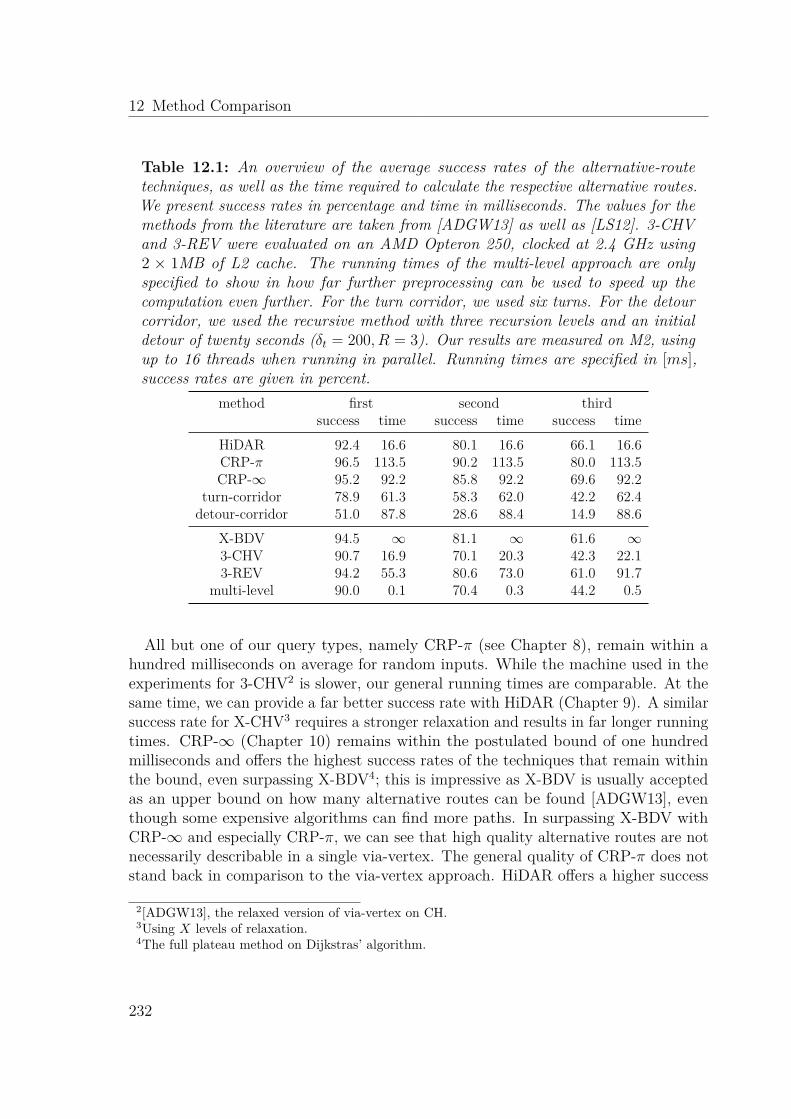
12 Method Comparison
Table 12.1: An overview of the average success rates of the alternative-routetechniques, as well as the time required to calculate the respective alternative routes.We present success rates in percentage and time in milliseconds. The values for themethods from the literature are taken from [ADGW13] as well as [LS12]. 3-CHVand 3-REV were evaluated on an AMD Opteron 250, clocked at 2.4 GHz using2 × 1MB of L2 cache. The running times of the multi-level approach are onlyspecified to show in how far further preprocessing can be used to speed up thecomputation even further. For the turn corridor, we used six turns. For the detourcorridor, we used the recursive method with three recursion levels and an initialdetour of twenty seconds (δt = 200, R = 3). Our results are measured on M2, usingup to 16 threads when running in parallel. Running times are specified in [ms],success rates are given in percent.
method first second thirdsuccess time success time success time
HiDAR 92.4 16.6 80.1 16.6 66.1 16.6CRP-π 96.5 113.5 90.2 113.5 80.0 113.5CRP-∞ 95.2 92.2 85.8 92.2 69.6 92.2
turn-corridor 78.9 61.3 58.3 62.0 42.2 62.4detour-corridor 51.0 87.8 28.6 88.4 14.9 88.6
X-BDV 94.5 ∞ 81.1 ∞ 61.6 ∞3-CHV 90.7 16.9 70.1 20.3 42.3 22.13-REV 94.2 55.3 80.6 73.0 61.0 91.7
multi-level 90.0 0.1 70.4 0.3 44.2 0.5
All but one of our query types, namely CRP-π (see Chapter 8), remain within ahundred milliseconds on average for random inputs. While the machine used in theexperiments for 3-CHV2 is slower, our general running times are comparable. At thesame time, we can provide a far better success rate with HiDAR (Chapter 9). A similarsuccess rate for X-CHV3 requires a stronger relaxation and results in far longer runningtimes. CRP-∞ (Chapter 10) remains within the postulated bound of one hundredmilliseconds and offers the highest success rates of the techniques that remain withinthe bound, even surpassing X-BDV4; this is impressive as X-BDV is usually acceptedas an upper bound on how many alternative routes can be found [ADGW13], eventhough some expensive algorithms can find more paths. In surpassing X-BDV withCRP-∞ and especially CRP-π, we can see that high quality alternative routes are notnecessarily describable in a single via-vertex. The general quality of CRP-π does notstand back in comparison to the via-vertex approach. HiDAR offers a higher success
2[ADGW13], the relaxed version of via-vertex on CH.3Using X levels of relaxation.4The full plateau method on Dijkstras’ algorithm.
232

12.1 Analysis
rate than X-BDV for the third alternative. This effect can be attributed to the order inwhich routes are chosen, though, as the previously selected routes impact the overlapfor further candidates. We study the effects of different route extraction strategies inthe next section.
Both corridor methods remain well within the postulated bound. The success ratesfor first and second alternative paths are too low to justify their usage as an alternative-route technique, though. Since our techniques are all based on the creation of a graphand run X-BDV on it, extracting a second and third alternative comes cheap. Only thegraphs created by the corridor methods are large enough to impact upon the runningtime in a noticeable way.
A Note on Possible Combinations. Some combinations of the techniques presentedhere seem rather logical. Bader et al. have already shown that the combination ofthe plateau method and the penalty method [BDGS11] offers better results thanthe methods on their own. The different underlying speed-up techniques prevent ancombination apart from uniting the final alternative graphs. While CRP-π and CRP-∞use the same technique, their results are too similar to show any significant benefit.The benefit of combining the plateau method, in form of HiDAR, with CRP-π hasalready been discussed by Bader et al. and is left out for this reason.
12.1.2 Path Extraction StrategiesAs previously shown in Figure 6.3, the strategy of how to select paths could potentiallyhave a large influence on the success rates and the quality of the found alternative routes.To check this influence, we performed a series of experiments, calculating success ratesfor the first three alternative routes, as well as their quality. For strategies, we orderedthe candidates in order of their quality with respect to the different parameters inDefinition 5.4. Finally, we also considered a linear combination of the different qualityparameters, as used in the publications of Abraham et al. [ADGW13] and Luxen andSchieferdecker [LS12]. For each of these strategies, we performed an extraction of upto three alternative routes on a thousand random pairs of source and target vertices.We summarize the results in Table 12.2.
Interestingly enough, the general selection strategy does not seem to impact uponthe success rates for finding a second or third alternative route. The strategy can havea large impact on the perceived quality of a path, though. In most cases, the results fora given method are consistent, offering similar results for all parameter values. Largevariations are possible, though, and sometimes are in the order of close to ten percent.One might say, though, that any reasonable strategy does not change the quality inan unreasonable way. Focusing on the optimization of a single value can result in aloss of quality for later alternatives; the overlap with selected routes may prevent thediscovery of other high-quality routes. Optimizing for a good BS for example yields aworse result on the third alternative than the optimization for limited sharing.
233

12 Method Comparison
Table 12.2: Success rates and parameter quality over different selection strategies.The strategies order candidates by a single parameter or a linear combination(F , equally weighting all three) of them. Depicted are the values for up to threealternative routes. The quality values of ML are inconsistent with the providedsuccess rates, as Luxen and Schieferdecker fail to provide a quality evaluation fortheir best success rates. The success rates for which the specified quality values arepresented in [LS12] are considerably lower (81.2, 51.2, and 25.0 percent). For thecorridors experiments, we used a six-turn corridor and a three-recursive detourcorridor with an initial detour of twenty seconds (δt = 200). The quality values for3-CHV and 3-REV are only specified for the first alternative. The ones for thesecond and third alternatives are taken from the non-relaxed versions.
method S first second thirdrate α β ε rate α β ε rate α β ε
CR
P-π
α 96.5 30.6 30.3 18.4 90.2 35.7 30.5 14.1 80.0 37.7 31.6 11.2β 96.5 50.1 50.6 11.4 90.2 51.8 47.7 11.5 80.0 42.4 32.7 12.5ε 96.5 52.0 61.0 6.7 90.2 44.8 39.5 10.9 80.0 38.3 26.5 12.4F 96.5 43.4 55.8 8.0 90.2 45.4 42.5 11.4 80.0 39.4 28.6 12.6
CR
P-∞
α 95.2 44.6 58.7 17.4 85.8 50.2 57.2 13.1 69.6 46.2 49.4 11.3β 95.2 59.9 83.0 9.2 85.8 55.2 65.4 10.7 69.6 41.1 43.7 12.4ε 92.5 56.8 82.3 5.8 85.8 50.6 58.6 10.8 69.6 42.0 42.1 14.6F 92.5 52.6 83.6 6.5 85.8 52.1 61.3 12.4 69.6 43.4 43.2 12.0
HiD
AR α 92.4 37.5 61.7 12.2 80.1 40.9 56.6 9.8 66.1 39.2 49.6 7.9
β 92.4 55.1 85.8 7.0 80.1 48.1 66.5 9.2 66.1 37.9 47.1 8.5ε 92.4 53.5 81.7 5.8 80.1 44.1 58.8 8.1 66.1 37.0 46.7 8.3F 92.4 48.5 82.5 6.3 80.1 43.3 60.1 8.2 66.1 37.0 46.0 8.4
turn
α 78.9 42.8 50.9 11.6 58.3 36.2 40.0 8.8 42.2 28.5 30.0 6.2β 78.9 50.1 69.2 6.5 58.3 37.1 4.3 9.3 42.2 26.2 24.5 8.1ε 78.9 48.9 67.0 6.4 58.3 35.3 3.9 8.4 42.2 27.4 26.5 6.2F 78.9 47.3 68.0 6.4 58.3 36.3 41.0 8.6 42.2 26.9 25.6 6.1
deto
ur
α 51.0 29.7 38.1 5.2 28.6 18.3 22.4 2.5 14.9 10.0 11.4 1.1β 51.0 32.2 46.2 2.4 28.6 17.9 20.3 5.0 14.9 9.2 8.9 1.4ε 51.0 31.6 44.8 2.4 28.6 17.8 20.6 2.1 14.9 9.5 9.6 3.7F 51.0 31.0 45.6 2.4 28.6 18.1 20.3 4.5 14.9 9.5 9.3 1.5
X-BDV F 94.5 47.2 73.1 9.4 80.6 62.4 71.8 11.8 59.6 41.2 68.7 13.23-CHV F 90.7 45.4 67.7 11.5 70.1 55.3 77.6 10.8 53.3 59.3 79.0 12.03-REV F 94.2 46.7 71.9 9.5 80.6 60.3 71.3 12.2 61.0 66.6 74.9 12.8ML* F 90.0 48.6 75.8 9.9 70.4 57.0 80.4 10.7 44.2 59.8 82.6 10.7
234

12.2 Quality Analysis
12.2 Quality Analysis
Next to the values for random queries, we also present information with regard todifferent Dijkstra ranks. This analysis discusses the quality of the different approachesfor different query types.
12.2.1 Alternative Graph ParametersIn addition to the considerations we already presented within the chapters, we nowcompare the different approaches with regard to their respective quality parameters.We omit the values for average distance, as they show very little variation. The valuesreach from 1.02 to 1.06, except for the corridors, which reach 1.1 for medium-rangedqueries. We depict values for total distance (Dtot) and the number of decision-arcsin Figure 12.1. Except for the corridors, which offer a very large number of verticesand arcs, HiDAR offers the best Dtot. We might extract alternative routes from thecorridor to get reasonable values for Dtot. The next section shows that the corridorsdo not offer better values than the other techniques, though. They do reach thesevalues, but only by ignoring the limit on decision-arcs, though. CRP-∞ can competewith CRP-π for most Dijkstra ranks, making it a viable replacement for low-range tomid-range queries. For ranks 221 through 224, Dtot remains far lower than with CRP-π.Given a similar number of decision-arcs, we can see that CRP-∞ finds shorter detours.
12.2.2 Route QualityNext to the alternative graph parameters, we study the quality of extracted routesas well. Here, we present the success rate for the first alternative route as well asits quality. The selection considers the first viable route according to a strategy thatselects the longest plateau first.
Success Rate. In terms of success rate, most methods show a very similar behavior.Figure 12.2 shows all but the corridor methods to offer close to the same success ratefor all Dijkstra ranks. For medium-ranged queries, the via-vertex approach is a bit lessgood than the other approaches. It surpasses the corridors starting at Dijkstra rank218 . As we stated in Chapter 6, this rank roughly represents queries of three hundredkilometers in length. In general, the penalty-based approaches offer the best successrates. They also require the largest computational effort, though.
The number of different choices that are available as a first alternative routes offersa more distinct picture. For short-ranged and mid-ranged queries, the general pictureremains the same. For long-ranged queries, however, HiDAR now surpasses CRP-∞.Especially the corridors methods offer only a few possible alternatives. Still, the mostcostly method offers the best results. CRP-πs offers up to two additional choices forDijkstra rank 224 .
235

12 Method Comparison
12
34
56
78
21 22 23 24 25 26 27 28 29 210 211 212 213 214 215 216 217 218 219 220 221 222 223 224
Dijkstra Rank
Tota
l Dis
tanc
e
● ● ●
●
●
●
●
●
● ● ●●
●
●
●
●
●
●
PenaltyExclusionHidarTurnDetour
01
23
45
67
89
11
21 22 23 24 25 26 27 28 29 210 211 212 213 214 215 216 217 218 219 220 221 222 223 224
Dijkstra Rank
Dec
isio
n A
rcs
●●
●
●
●●
●
●
●
●
PenaltyExclusionHidarTurnDetour
Figure 12.1: Alternative Graph Measures
236
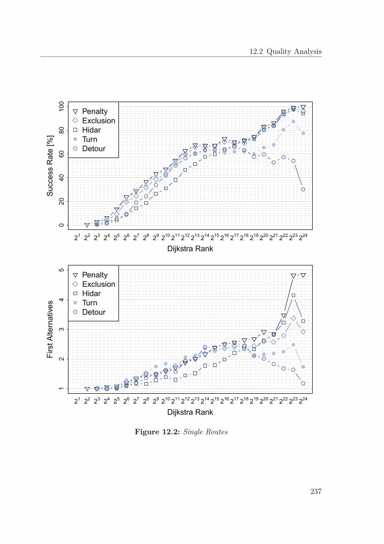
12.2 Quality Analysis0
2040
6080
100
21 22 23 24 25 26 27 28 29 210 211 212 213 214 215 216 217 218 219 220 221 222 223 224
Dijkstra Rank
Suc
cess
Rat
e [%
]
● ●●
●
●
●●
●●
●● ●
● ● ● ● ●●
●●
●
●
●
● ●●
●
●
●
●
●
●
●●
● ● ● ●●
●●
●●
●
●
●
●
PenaltyExclusionHidarTurnDetour
12
34
5
21 22 23 24 25 26 27 28 29 210 211 212 213 214 215 216 217 218 219 220 221 222 223 224
Dijkstra Rank
Firs
t Alte
rnat
ives
● ● ● ●● ●
●●
●●
● ●
● ●● ● ●
● ● ● ●
●
●
● ● ● ●●
●●
● ●
● ●
● ●● ●
●
●●
●● ●
●
●
●
PenaltyExclusionHidarTurnDetour
Figure 12.2: Single Routes
237

12 Method Comparison
020
4060
8010
0
21 22 23 24 25 26 27 28 29 210 211 212 213 214 215 216 217 218 219 220 221 222 223 224
Dijkstra Rank
Loca
l Opt
imal
ity [%
]
● ● ● ● ● ● ● ● ●●
● ● ● ● ● ● ● ●● ● ●
● ●
● ● ● ● ● ● ● ●●
● ●● ● ● ● ● ● ● ● ●
● ●
●
●
PenaltyExclusionHidarTurnDetour
Figure 12.3: Quality according to Definition 5.3.
020
4060
8010
0
21 22 23 24 25 26 27 28 29 210 211 212 213 214 215 216 217 218 219 220 221 222 223 224
Dijkstra Rank
Sha
ring
[%]
●
●
● ●
●● ●
●● ● ●
● ●● ● ● ● ● ● ●
●●
●
●●
●●
● ● ● ● ● ● ● ● ● ● ● ● ● ● ● ● ●
●●
●
PenaltyExclusionHidarTurnDetour
Figure 12.4: Quality according to Definition 5.3.
238

12.3 Conclusion0
24
68
1114
1720
23
21 22 23 24 25 26 27 28 29 210 211 212 213 214 215 216 217 218 219 220 221 222 223 224
Dijkstra Rank
Stre
tch
[%]
● ●●
●●
●
●●
●
●● ● ●
●
● ●●
●● ●
●
●
●
● ● ●●
●●
●
●
●
● ● ● ●● ● ● ●
●
●
●●
●
●
●
PenaltyExclusionHidarTurnDetour
Figure 12.5: Quality according to Definition 5.3.
Stretch. Similar to the values in Table 12.2, the values for bounded stretch (BS)are comparable for most of the Dijkstra ranks. For long-range queries, penalizationmethods offer larger BS, though.
Local Optimality. Optimizing for long plateaux means essentially optimizing forlocal optimality (LO). As a result, we see the largest differences between our methods inFigure 12.3. Penalization tends to find paths that offer far lower values for LO. CRP-∞is closer to HiDAR, though, than the classic form of penalization. This indicates routescalculated by CRP-π might try to avoid the shortest path too strongly.
Sharing. On average, most techniques offer very little variation in terms of sharing.This depends on the selection strategy, though, as we can see when comparing to thevalues in Table 12.2. The wide range of possible strategies make it impossible to give acomplete overview.
12.3 Conclusion
We have discussed five different methods of computing alternative routes for staticgraphs. These methods offer an interesting selection of possible routes that can becalculated using speed-up techniques or parallel processing. As with the general
239

12 Method Comparison
underlying problem itself, none of the techniques can be claimed as superior in allaspects. While corridors seem to be reasonable with respect to their initial goal, theother techniques in form of CRP-π, CRP-∞, and HiDAR offer their own benefits. Allof them can be considered as alternative algorithms to compute alternative routes.
Our algorithms offer very good success rates and can also be used to discover routesof higher quality. For commercial systems, there exist a lot of topics for furtherstudies. All CH-based methods offer a problem in terms of consistency. Whenever thepreprocessing is redone, the order of contraction may change. As a direct result, thediscovery of via-vertex may change and offer non-deterministic results.
A penalization approach, as in CRP-π or CRP-∞ – a variant that may be possibleto implement on a CH as well – can alleviate this problem. A via-vertex, given therestrictions usually imposed, is arguably a viable choice for an alternative route, though.The same can, however, not be said as easily for a penalization approach. Any smallsegment on a penalized path can, if it is unreasonable, result in unsatisfied customers.
In addition, all techniques offer less possibilities than we would expect in general.Especially the success rates for low-range and mid-range queries should be increasedto better cover the most common queries. Possibly, a combination of several of theproposed techniques might be useful. It is doubtful, however, that a multi-techniqueset-up is sustainable in a commercial system. In addition, the idea of what mightconstitute a good alternative route might have to be reconsidered. Current qualitycriteria are mostly motivated by the techniques they were introduced with first.
In terms of running times, we cannot compete with the currently fastest approachof Luxen and Schieferdecker. Taking preprocessing overhead into account, we simplyoffer a different trade-off.
Using more time in the query, penalization as done in CRP-π and CRP-∞ offers aninteresting addition to the field of alternative routes. Our implementation is the firstone to allow for interactive queries on continental networks. The improved successrates over the full plateau method (X-BDV) indicate that more versions of reasonablealternative paths exist than the classical via-vertex approach might make think. Apossible example to consider might be to search for multi-hop routes: instead ofcomputing the concatenation of two paths, we might consider a list of intermediatevertices.
240

Part III
Further Studies
241


13 Chapter 13
On Stochastic On-Time Arrival
In the presence of uncertainty, optimal routing requires a good strategy. Thischapter discusses possible further applications for alternative route techniques inan advanced scenario. The implementation presented in this paper is supportedby a wrapper for the fftw library, written by Dennis Schieferdecker. Thelibrary is used to speed-up the convolutions required in the following setting.The code for the stochastic on-time arrival problem (SOTA) algorithm is areimplementation of my own, written during fruitful discussion with SamithaSamaranayake.
The most typical metric used in the SPP is the travel time metric, which considersthe average expected travel time along a path. This metric should, normally, providethe fastest means of traveling from a source to a target. But Metrics only consideringa single value offer only a rather simplified view of the real world, as this standardassumption of a static road network does not represent known dynamic influences. Atypical example of such a parameter can be found in the recurrent delays during therush hour that result in slow-moving traffic or even traffic jams on many importantroad segments.
In general, we can distinguish between two types of delays that occur in road networks:regular delays and irregular delays. Regular delays can be identified, to a certaindegree, via a series of measurements; remember Figure 6.2 for a comparison. At certaintimes of the day, heavily used roads are crowded due to regularly occurring demandlike the commute to and from work; as a result, we can find re-emerging patterns overthe course of a week. These patterns manifest themselves in slower travel times forcertain road segments during the rush hour in comparison to the ones experiencedduring free flowing-traffic. These types of changes are subject to the research done ontime-dependent route planning. For a thorough discussion of the subject, we refer to[Bat14].
We know of only a single study that discusses the merits of considering times of high
243

13 On Stochastic On-Time Arrival
or low traffic density in navigation systems [DBKS10]. The improvements claimed bythe authors seem a bit high in our eyes, though, and seem to result in a comparison ofroutes in the time-dependent model against routes calculated for free-flowing traffic.A consideration of the on average expected travel time would probably reduce theimprovements gained by the consideration of time-dependence severely. We see asimilar effect in our algorithms that show significantly different results if we considerfree-flowing traffic instead of expected travel times. In addition, the model used inthe study seems to contain simulated data and lacks verification in form of an actualuser-study. Besides this study, no further discussions of the merits of time-dependentroute planning are known to us.
In the second type of delays, the research community considers a form of irregulardelays that cannot be pinpointed to a specific recurring pattern. These irregulardelays can result from a car in a narrow road during a parallel parking maneuver, agarbage truck or some other delivery vehicle blocking a road. In addition, many otherforms of unpredictable behavior that can affect the road network are possible. Theseuncertainties can also be used to model effects of traffic lights, stop signs or any othertraffic guidance method that can result in a stop. All of these potentially long delayscan be expressed as a probabilistic delay, associated with the road segments.
Handling these stochastic delays is a difficult task, though, and an exact computationmight not always be required.
Our final contribution is split into two sections. In the upcoming section, we describethe general problem of the stochastic on-time arrival problem problem. We alsointroduce the algorithms currently used to solve it.
Afterwards, we discuss our own contribution: We postulate that even complexproblems in road networks often reduce to a set of meaningful alternative routes.For example, attached components next to a road will never contribute to a viablerouting strategy. By reducing the algorithms for difficult problems to work on a smallersub-graph, we can significantly impact the performance of these algorithms. Eventhough this method lacks any approximation guarantees, we show in an experimentalstudy that they offer viable approximations nonetheless. We present these results inthe context of an algorithmic study, without introducing tailored algorithms.
13.1 Problem Definition and Baseline Algorithm
The literature mainly distinguishes between two different ways of considering unreliabletravel times: shortest path with on-time arrival reliability (SPOTAR) and the SOTA1,the latter being the main topic of interest in this chapter. Both techniques operateon a limited travel time budget. SPOTAR is targeted at an optimal a priori paththat maximizes the probability of on-time arrival. A solution to this problem is due
1Different settings considering reliability of the computed paths exist. Examples of different ap-proaches are [CBWB06, CBB07].
244

13.1 Problem Definition and Baseline Algorithm
to Nie and Wu [NW09] who consider the first-order stochastic dominance of paths.The optimal solution is not viable due to potentially exponential running times in theworst-case; Nie and Wu present a pseudo-polynomial algorithm for an approximatesolution that performs well in practice. For a restricted version that considers Gaussiandistributions, Nikolova et al. [NKBM06] show how to find a solution in O
(nΘ(log n)
).
We discuss the second approach in the following sections.
13.1.1 The SOTA problem
The stochastic on-time arrival problem problem aims at the calculation of an on-linestrategy to guide a driver, rather than the calculation of a single a priori path. Sucha strategy denotes a next vertex for every budget that the respective vertex can bereached with, given a fixed starting budget. This allows for a dynamic adjustment ofrouting directions, depending on previously experienced travel times. The resulting(expected) success rate of a driver following the SOTA strategy is guaranteed to beequal to or higher the probability of SPOTAR.
Formally, the SOTA problem is defined as follows:
Definition 13.1 (stochastic on-time arrival problem (SOTA) problem). We consider agraph G (V, A) and for every arc a ∈ A a cost-function μa (·) in the form of a probabilitydensity distribution; the distributions themselves are considered independent of oneanother. Given a time budget T , a source s and a target t, find an optimal routingpolicy that maximizes the probability of reaching t within the time budget T . Such arouting strategy determines the optimal next vertex to travel to, based on the remainingtime budget due to the previously realized travel time. Let pv,t [T ] denote the probabilityof reaching t from v within the budget T . A solution to the optimal routing policy isdescribed in the equations, given 0 ≤ τ ≤ T :
pv,t [τ ] = maxa=(v,w)∈A
∫ τ
0μa (ω) pv,t [τ − ω] dω, ∀u ∈ V \ {t} (13.1)
pt,t [τ ] = 1
succv,t (τ) = arg max(v,w)∈A
∫ τ
0μa (ω) pv,t [τ − ω] dω, ∀u ∈ V \ {t} (13.2)
Fan and Nie [FN06] formulate the SOTA problem as a dynamic programmingproblem, solving it with a Successive Approximation algorithm. Their algorithmcannot be bounded in a finite number of steps, though, when the network containscycles [SBB12a]. In the SOTA setting, such a cycle can be part of an optimal strategy.An example for such a case is presented in Figure 13.1. Figuratively speaking, ina solution to the SOTA problem we compute a SPOTAR path in advance for anyremaining budget and every possible vertex we might end up at during a journey.
245

13 On Stochastic On-Time Arrival
s t
v
10010
15090
120100
290
2010
2100
(a) Graph
2010
s t
v
10010
15090
120100
290
2100
(b) SPOTAR
15090
s t
v
10010
120100
290
2010
2100
(c) SPOTAR at v, rem. budget 110
s t
v
10010
15090
120100
290
2010
2100
121
119∞
99
101
ts⊥
⊥tv∞
(d) SOTA strategy
Figure 13.1: A small example that contains a cycle in the optimal strategy. Letthe budget for the travel be 130. Arc weights are specified in the boxes, each stackgiving a time and the probability of experiencing this time in percent. The SPOTARpaths (13.1b, 13.1c) show the contributing parts of the respective arcs. For theSOTA strategy, we give the next vertex in dependence of the remaining budget.
To deal with such cycles, Nie and Fan propose a discrete approximation algorithmthat converges in a finite number of steps and is running in pseudo-polynomial time[NF06]. Under the reasonable assumption of a strictly positive minimum weight over allarcs (μ (a ∈ A) > 0), Samaranayake et al. [SBB12a] present a number of optimizationtechniques like a label-setting algorithm and advanced convolution methods centered onthe idea of Fast Fourier-Transformations(FFTs) by zero-delay convolutions [SBB12b].
The structure of the problem prevents the direct application of the techniques dis-cussed in Chapter 4; a main reason for this is the inclusion of loops in an optimalstrategy. Nevertheless, some form of pre-processing is still possible. Sabran et al.[SSB14] manage to employ versions of reach and ArcFlags to speed-up the computa-tion. The success of the techniques ranges from little improvement, speeding up thecomputation by a few percent, to close to an order of magnitude. These techniquesrequire close to a day running time, though, even on very small graphs.
The difficulty of this problem is our main reason to consider it in the connectionwith alternative routes. Whereas a connection between a reasonable path as consideredin the SPOTAR model and a set of meaningful alternative routes seems plausible, the
246

13.1 Problem Definition and Baseline Algorithm
same cannot be said immediately for the connection with an online SOTA strategy.The main difference between a path in an alternative graph and the SOTA strategyis the inclusion of cycles in the latter. For a viable alternative path, we postulate asimple path by employing the criterion of local optimality. In SOTA, the optimalstrategy depends on the possibility to turn around at any given location. As a result,the two approaches offer some considerable structural differences. Nevertheless, ourstudy shows that alternative route techniques can offer a viable approximation choicefor such a difficult problem.
13.1.2 Baseline Algorithm
Before coming to the discussion of our main topic, i.e. in how far alternative routetechniques can be applied to the SOTA problem, we introduce the baseline algorithmand its main principles.
Discretization As the basic problem can be seen as a continuous problem, it doesnot seem reasonable to consider higher resolutions than the resolution considered instatic route planning, especially, as the probabilistic model itself can only be seen asan estimate. A fully continuous interpretation of the problem is not beneficial, as weare limited in the resolution anyhow. We denote the discrete interpretation of thecontinuous functions in the use of square brackets ([·]) over parenthesis in the formulas.
The optimal order algorithm. As we have already mentioned, the equations (13.2)can be solved using Successive Approximation [FN06]. Samaranayake et al. [SBB12a]present an algorithm for finding the optimal solution to the SOTA problem in a singlepass through the time-space domain. The only requirement is the previously mentionedassumption of a strictly positive lower bound for the cost of an arc. Let uk
v [t] denotethe Cumulative Distribution Function (CDF) that denotes the probability of reachingthe target t from v in at most k steps: Algorithm 13.1 describes the method presentedin [SBB12a].
The computation of the CDF cannot be computed analytically; the form of apointwise maximum over the adjacent arcs and their associated convolutions preventsit. We can improve on algorithm 13.1 by considering not just the minimum realizabletravel time at an arc connected to a vertex but also the length of the shortest possiblecycle which contains it. The proof can be found in [SSB14], but the idea behind itis rather simple: assume for any link a = (v, w) that we have computed uw [·] up tosome budget τw . Due to the minimal possible travel time between v and w of δv,w, wecan update uv [·] up to the budget of τv ≤ τw + δv,w . Now consider a shortest cyclev = v0, . . . , vk = v of length δv = ∑k
i=1 δvi−1,vithat v belongs to. Stepping along the
path, we update each uvi[·] by a delta of δvi−1,vi
before arriving back at vk = v . Dueto the updates along the path, we update uv [·] by δvk,vk−1 , completing the circle. The
247

13 On Stochastic On-Time Arrival
Algorithm 13.1 Single Pass SOTAInput: A graph G (V, A), a metric in the form of probability distributions (p [·]), a
source s, a target t, a time budget TOutput: An optimal routing strategy from s to t that respects T
1: δ = mina∈A τa, τa = minτ : pa [τ ] > 0 � Minimal realizable travel time2: kmax = �T/δ� � The number of steps3: u0
v [τ ] = 0, ∀v ∈ V, v = t, τ ∈ [0, T )4: u0
t [τ ] = 0, τ ∈ [0, T )5: for k ∈ [1, kmax] do6: τ k = kδ7: uk
t [τ ] = 0, τ ∈ [0, T )8: for all v ∈ V, v = t do9: uk
v [τ ] = uk−1v [τ ] , τ ∈
[0, τ k − δ
]10: uk
v [τ ] = uk−1v [τ ] , τ ∈
(τ k − δ, τ k
]11: uk
v [τ ] = maxa=(v,w)∈A
∫ t0 pv,w [ω] uk−1
w [τ − ω] dω, τ ∈(τ k − δ, τ k
]12: end for13: end for14: return uk
i [·]
total increase of τi is therefore given by δi . The process, however, is dependent on theorder in which the vertices are processed (compare Figure 13.2). Whereas the updatesin topological order (see Figure 13.2c) increase the respective τi values by δi = 11 ,updates in reverse topological order behave less well (Figure 13.2b).
To determine the best possible order to process the vertices in, Samaranayake et al.[SBB12a] discuss an algorithm related to Dijkstra’s algorithm (compare Algorithm 2.2and Algorithm 13.2). The algorithm processes the elements by a reverse pass throughthe time-space domain. Beginning at the source, for which the CDF has to be computedup until the target budget, the algorithm iteratively computes the most constraintvertices. The most constrained prerequisite, i.e. the vertex that is required to be knownup to the largest budget, is selected next and added to the (reverse) order. For thisprocess, the algorithm maintains a max heap that contains the most restricted elements;we present a pseudo-code for this approach in Algorithm 13.2.
An example: If we were to compute the best order for the graph shown in Fig-ure 13.2a to get from b to t with a budget of 30, the order algorithm would yield(b, 30), (c, 25), (a, 23), (b, 19), (c, 14), (a, 12), (b, 8), (c, 3), (a, 1) . The reversal of this orderyields a → c → b , the same order as processed in Figure 13.2c. The target t is omittedin this process as its complete CDF is known in advance and provides the base case.
248

13.1 Problem Definition and Baseline Algorithm
ta
b
c
1
4
2
5
(a) graph
Iter. a b c1 1 5 22 9 7 33 11 8 11
(b) a → b → c
Iter. a b c1 1 8 82 12 19 143 23 30 25
(c) a → c → b
Figure 13.2: Updates of the τi values over the course of the SOTA algorithm fora small cyclic graph.
Algorithm 13.2 Order AlgorithmInput: A graph G (V, A), a metric in the form of minimal realizable travel times
(μ), a source s, a target t, a time budget TOutput: An optimal order for the SOTA algorithm to process the vertices in
1: O = ∅2: Q = {(s, T )}3: while Q = ∅ do4: n = (v, τ) = maxτ Q � get most constraint vertex5: Q = Q \ {n}6: O = O ∪ {n}7: for all w : (v, w) ∈ A, w = t, τ − δv,w > 0 do8: τw = max(Q.getKey(w), τ − δv,w)9: Q.updateKey(w, τw) � insert w if not already contained
10: end for11: end while12: return O
Zero Delay Convolution. During the process of the baseline algorithm, we requirethe continuous evaluation of CDFs from the CDFs of neighboring vertices and theprobability density functions assigned to the respective arcs. The probability densityfunctions pa∈A [·] are fixed and can be evaluated in advance. The former parameter,however, is continuously updated over the progress of the algorithm. To avoid un-necessary calculations, Samaranayake et al. propose the usage of so-called zero delayconvolutions: a FFT-based method for calculating convolutions between a fixed variableand a continuous stream.
The method considers two vertices i and j as well as the arc a := (i, j) between themin the following way: Given the CDF uj and the probability density function pa [·], theCDF ui can be calculated as ui [k] = ∑k−1
l=1 uj [l] pa [k − l] , ∀k . Dean [Dea10] shows thatZero-Delay Convolutions(ZDCs) can be applied to SOTA to reduce the computationaloverhead at each link, due to the convolutions, from O (T 2 log T ) to O
(T log2 T
). While
the straightforward approach for a convolution requires an effort quadratic in the number
249

13 On Stochastic On-Time Arrival
uj [1]pa [1]uj [1, 2] ∗
pa [2, 3]uj [3, 4] ∗
pa [2, 3]uj [5, 6]
pa [2, 3]uj [7, 8]
uj [1, 4]
∗pa [4, 7]
∗uj [5, 8]
ui [2]
uj [2]pa [1]uj [3]pa [1]uj [4]pa [1]uj [5]pa [1]uj [6]pa [1]uj [7]pa [1]uj [8]pa [1]uj [9]pa [1]
ui [3] ui [4] ui [5] ui [6] ui [7] ui [8] ui [9] ui [10] ui [11]
Figure 13.3: Illustration of a ZDC based arc relaxation under the assumption thatthe vertices i and j are connected by a single arc. At the computation of ui [k], weonly require access to values of uj [k − 1] and other earlier values. We can extendthe size of the convolution blocks when the minimum cost of an arc is larger than 1 .
of discrete values (O (T 2)), FFT can compute such a Discrete Fourier-Transformation(DFT) in O (T log T ) (ui [k] = (uj [·] ∗ pa [·]) [k]). The algorithm requires access to allvalues, though. Given that the probability density function pa [·] can be evaluated forany k, we can compute ui [k] as a sum of multiple DFTs. The basic motivation behindthis approach is to utilize FFTs as much as possible.
Some values are easy to compute. For example, given μ (a ∈ A) > 0, we findui [1] = 0 and ui [2] = uj [1] · pa [1] . For the computation of ui [3] , we need to calculateui [3] = uj [2] pa [1] + uj [1] pa [2] with the latter equal to (uj [1, 2] ∗ pa [2, 3]) [1] . Theremaining entries at positions two and three of this DFT are part of ui [3] and ui [4] andcan be used as such. As a result, we only require a single additional value (uj [3] pa [1])to compute ui [4] . The more values of uj become available over the course of thealgorithm, the larger the possible FFTs tasks become; see Figure 13.3 for an illustration.All values of uj [·] required during the computation of ui [·] are of a smaller index.
The metric assigned to the problem, defining a minimal realizable travel time (δ)along an arc, enables us to reduce the computational overhead even further by employingδ-multiple ZDC. The factor δ allows for larger blocks of convolutions to be handled at atime, reducing the computational cost from O
(T log2 T
)to O
(T · (log2 T
δ))
[SBB12b].
13.1.3 Correctness Preserving Pruning TechniquesIt is rather obvious that the algorithm for the computation of an optimal SOTAstrategy, even when using ZDC in combination with FFTs and the optimal order,remains a very costly process. Without sacrificing correctness, we can prune somevertices from being considered in the optimal order.
Lower Bounds. Given an optimal traversal of an arc during free-flowing trafficwithout any delays, the time taken for the traversal marks a lower bound. If weconsider only these lower bounds during an instance of Dijkstra’s algorithm, it becomes
250

13.2 Contribution: Alternative-Route Pruning Techniques
obvious that any budget below the minimal realizable travel time evaluates to zeroin terms of its probability of reaching the target on time. The same can be said forvertices that do not offer a combined travel time of D (s, v) + D (v, t) > T . These donot have to be considered during the calculation, as they cannot contribute a positivevalue to the CDF at the source vertex.
Upper Bounds. The discretization in our interpretation allows for upper bounds aswell; they are usually not considered, as we expect the maximal allowed budget to belower than the upper bound anyways. For every distribution we find some 100 − ε2
percent quantile, giving a guarantee in some sense to traverse the arc in the giventime. This is an approximation, but can be easily justified by the inaccuracy of theunderlying model. The travel time that gives this 100 − ε percent chance to traversethe arc is assumed as the maximal cost of the arc. Again, utilizing Dijkstra’s algorithm,we can set uv [τ ] = 1, ∀τ ≥ D (v, t) with respect to this maximum metric. This alsoenables us to directly adjust the time-space domain in case the initial budget hasbeen chosen too large. This is technically an approximation; the measurement-basedprocess of determining the respective probability distributions is an approximationto begin with, though, too. Given the nature of the utilized distributions, a routingalgorithm would end up considering up to a day’s worth of budget when it comes totraversing a city the size of Stuttgart or San Francisco. This scenario is both unrealisticand undesirable. In terms of the comparison we consider later in this chapter, thisrestriction only speeds up the baseline algorithm and does not benefit our consideredpruning methods.
13.2 Contribution: Alternative-Route PruningTechniques
After our description of the baseline algorithm, we present our own contributions forpruning the SOTA algorithm.
The main justification for our approach is given in Figure 13.1. As one can see, theoptimal strategy given by the SOTA algorithm can be interpreted as the specificationof a SPOTAR path for any remaining budget at every reachable vertex. The goalof the SPOTAR model is to find the path with the highest probability of arrivingwithin the given time frame. In the SOTA model, we, figuratively speaking, preparefor any possible outcome and compute a SPOTAR path for every vertex we couldend up at with all possible remaining budgets. We encode this in specifying thenext vertex to travel to for any potentially remaining budget. At the source, we canimagine that the first vertex proposed by the strategy corresponds to the solution tothe SPOTAR problem. As long as we do not experience any delay, the path should
2We use ε = 0.001 to calculate the 99.999 % quantile.
251

13 On Stochastic On-Time Arrival
s
t
(a) Network
δ
s
t
(b) Unique
v
ab
δ
s
t
(c) Alternatives
Figure 13.4: Reasoning behind the alternative-route approach: consider a long-distance route from s to t. Apart from local adjustments, it is unlikely that we haveto leave the SPOTAR path at any point. Consider the scenario of a unique shortestpath. When traveling along it, a small delay can hardly be corrected in anythingbut a local fashion. In the presence of multiple possibilities, we expect a changebetween those only if one is slower but more reliable and the other one faster butless reliable. If we find a large enough delay (indicated by δ) at some point thatresults in a different path specified by the SOTA strategy, the new path (indicatedby b chosen over a) cannot be fully unreasonable but rather has to be a good pathas well for the rest of the journey.
continue to offer the maximal chance of arriving on time. The moment the budgetchanges unexpectedly, due to some random occurrence along the way, we would haveto overthrow our initial decision and rethink the directions by computing the mostreliable path for the currently remaining budget. This new path, however, cannot becompletely unreasonable as well. Assuming that all paths that can be considered bySPOTAR are from a set of reasonable alternatives, we can approximate SOTA withour own techniques.
If we consider a situation as depicted in Figure 13.4, we follow a path from s to t. Atsome point we might experience (or have accumulated) some delay. In many cases, thisdelay should not change the general direction of travel, at least during long-distancetrips. The reasoning behind this argument is that the natural hierarchy of a roadnetwork restricts long-distance travel to a small subset of important roads. If we travelalong a highway and consider static and independent probabilities, a change in theshortest path to follow is unlikely 3.
3We consider this a potentially oversimplified view, as the probability of a delay in close proximityto a traffic jam increases dramatically.
252
13.3 Experimental Study
For the most part, we would expect a strategy to follow slower but more reliablepaths, unless the budget gets too small. When the budget gets reduced below a certainsize, faster and potentially unreliable paths become the only possible choice.
In our example, a potential change in directions depends on the remaining budget.As long as a reliable, but slow, path (e.g. the one labelled a in Figure 13.4c) remainswithin the budget, it presents the path of choice. After an experienced delay, however,the budget might not be sufficient to a travel along the initially chosen path a and thestrategy presents b as the alternative path to follow. This kind of change is associatedwith a faster but potentially less reliable path. Completely ignoring the higher roadcategories at this point is not an option, as the travel time would increase significantly.In addition, roads of similar categories in close vicinity to each other should be roughlyequivalent in terms of their reliability.
Similar reliability on identical road types allows to exploit the natural hierarchyof the network in some sense. In fact, our experiments show that for the most partwe can restrict the search to a reasonable sub-graph without sacrificing much interms of correctness. This approach does not offer any guarantees of correctness,though. We only present it as a potential use case for alternative-route techniques. Weassume that, even in other settings, the general structure of reasonable routes does notdeviate completely from shortest paths with respect to travel time metric. This ideais motivated in the fact that travel time will always be one of the major factors andcannot be ignored completely.
Pruning Model. Given the parameterization of SOTA, pruning the algorithm usingthe alternative graph DAGs is not viable. Instead, we prune on the basis of vertices.This enables the strategy to hop between neighboring paths and to perform u-turns.However, this model affects the potency of attached component filtering for corridors.Since our test graphs contain only cities, the density within the network and the vertex-based pruning result in next to no attached components. For long-range travels, thecomponent filtering might offer great improvements. Unfortunately, we were not ableto obtain any reasonable probability data for larger graphs. Some tests on randomlygenerated data show promising results, though.
13.3 Experimental Study
The main goal of this study is an experimental evaluation of possible applications forour previously implemented alternative-route techniques. Therefore, we do not presentany new algorithmic approaches or techniques specifically tailored to the scenario.
We compare two different settings. The first one is the original SOTA algorithmwithout any application of additional pruning techniques. The second scenario considersthe original SOTA method restricted to a set of preselected vertices. For the selectionof these sub-graphs, we test a variation of alternative-route techniques.
253

13 On Stochastic On-Time Arrival
Standard of Comparison. While it is rather easy to quantify the decrease in qualitythat we can experience using our approximation-based methods, the same cannot besaid for the benefits. The decrease in quality can be measured in the CDF at thesource over the full range of the budget from minimal necessary budget to guaranteedarrival. We present both average values describing the full interval and error valuesscaled to a range from zero to a hundred percent of the budget range.
Unlike the objective measure of probability in the CDF, the measure of running timeis too dependent on the actual implementation choices made during the implementationof the SOTA algorithm. We still present some values for comparison, even though wefeel that they might favor our method too strongly.
To potentially give a better impression of our results, we focus on the number ofperformed convolutions. While this unit of measure is not an optimal one either, itdescribes the workload of the algorithm and is independent of other implementationchoices.
Next to the approximation of the CDF at the source, we present an additionalmeasure. This measure describes how well an optimal a-posteriori pruning set would becovered by the respective strategy. This set, which is introduce shortly in the followingsection, contains all vertices that are part of an optimal SOTA strategy.
13.3.1 Pruning Techniques
For completeness, we give a short overview of the different pruning methods we evaluatein this chapter. All of these techniques are used to select a set of vertices. Since it isunclear at which positions we might want to turn back, we do not limit this possibility.
The success of the SOTA strategy is reduced significantly if we only consider pathsthat are directed at the target. Since our alternative graphs define DAGs, a lot of thepotential benefits of a SOTA strategy would be lost.
Basic SOTA. The most basic version of the SOTA algorithm is the unpruned version.While of course employing upper and lower bound pruning, it does not use anyadditional pruning. This version represents our standard SOTA algorithm.
Optimal Pruning. Optimal (a-posteriori) pruning is what we call our referencealgorithm for a pruned SOTA instantiation. It is a rather theoretical construct, asit requires a full SOTA query and as such cannot possibly help in speeding up itscomputation. The method first executes the unpruned version of the algorithm. In asecond step, we traverse the computed SOTA strategy and extract all vertices thatcontribute to the CDF of the source vertex. This set of vertices is considered foranother run of the SOTA algorithm.
Even though it might not seem so at first, this method could potentially be restrictedfurther without any loss of quality. The method does not prioritize equivalent paths
254

13.3 Experimental Study
in any way. If the SOTA strategy contains references to multiple choices of the samequality, all of them are considered in the pruned version as well. It can be seen rathereasily that this restriction does not lower the quality of the found CDF at the source.By eliminating vertices that did not contribute to the final result in the first place, weonly eliminate an unnecessary workload.
The acquired set of vertices provides an idea of the actually workload required tocompute an optimal strategy. The vertices found this way are also used to measurehow well the other techniques replicate this information.
Corridor Pruning. As a first method of pruning, we employ unmodified versionsof our corridor algorithms. All vertices within the corridor are selected as pruningvertices. The amount of vertices is, however, far larger than suitable. Our differentmethods offer a vast choice for configuration, though. For a tailored method, the actualdistributions at the different arcs could be used to restrict necessary deviations. Wecould create a corridor that limits deviations to parts of the graph in which they arelikely. In addition, we could consider more deviations when we are in closer to thetarget, as the expected delay increases over the time of travel.
The dense corridors contain a far larger amount of circles than the other techniques.Therefore, this method should also reduce the amount of computation less than whatwe expect from other techniques. We consider multiple-turn versions of our corridorsand the recursive detour variant. The graphs tested offer only little potential to reducethe standard corridor in its size; due to the density of the graph, a corridor containsbarely any attached trees. We would expect these components to be of greater relevancein long-range queries, though.
Alternative Route and Graph Techniques. For the alternative-route/graph-basedpruning techniques, we consider the full set of possible choices. We extract every routethat might contribute a possible alternative path. The combination of these differentpaths forms our pruning set.
For the via-node-based methods, we consider the reference technique X-BDV toavoid any artifacts due to the underlying CH. Instead of only selecting a set of differentpaths, we consider the full set of plateaux, just as done in HiDAR. This way we donot only consider all potentially viable alternative routes, but also smaller deviationsthat would not make a reasonable alternative on their own. We discard all paths,though, that do not reach a plateau that would be long enough to pass the test forlocal optimality.
In the penalty-based approach, we use the upper-bound graphs that we introduced inSection 8.2.2. These graphs consider all paths found during the different penalizationiterations, ignoring the viability of segments and decision arcs. We limit the iterationsby our usual criteria, though, to keep the processing overhead manageable, performingabout ten penalization iterations.
255

13 On Stochastic On-Time Arrival
Table 13.1: Computational overhead of the SOTA algorithm in comparison to aperfect pruning strategy.
unpruned perfect pruning reduction factorgraph steps vertices steps vertices steps vertices
Stuttgart 11 302 276 48 462 74 822 318 0.01 0.007San Francisco 111 348 4 166 1 449 72 0.04 0.045
13.4 Evaluation
First, we take a look at the optimal pruning method. When we compare the workloadfor the general SOTA algorithm with the a-posteriori optimized version, we can seethat most of the work performed does not yield any improvements. Only a fraction ofthe actually processed vertices contribute to the final CDF at the source. Most of theconvolutions that SOTA performs can be pruned. Compare Table 13.1 and Figure 13.5in this regard.
The data shows that the results follow a similar pattern, no matter whether we areconsidering measured data (San Francisco) or simulated data (Stuttgart). The optimalstrategy is only concerned with a minor fraction of the initially generated prune-spaceand calculation order.
In our visualization of a perfectly pruned search, the motivation behind our ideato use alternative-route techniques becomes apparent. Along a shortest path, someadditional arcs may provide a choice for some budget values. Most of the vertices inthe search space of the SOTA algorithm do not contribute to the result, though. Eventhough they could theoretically offer a benefit, the mostly uniform behavior we expectin a road network manifests itself in only minor detours close to the shortest path.Only in a few cases, the search departs from the shortest path and follows anotherpath. The different path resembles a viable alternative route, though.
Turning to Figure 13.5, we can spot a close resemblance to the previously introducedcorridors. In comparison to Figure 11.6, we can instantly make out a lot of similarities4.In the following paragraphs, we compare the results we get from executing differentalternative techniques to prune the SOTA algorithm with the optimal algorithm.
Table 13.2 indicates the best approximation for our corridor variants. This is alsoconfirmed in Figure 13.6. The corridors offer very small average and maximal errorswith a low variance. The direct alternative variants, offer a good approximation onaverage. In spite of the good average quality, the worst case results are significant,though. If we compare the penalty method to the via-vertex approach, we get a verylarge difference in the number of vertices which we have to consider. However, for the
4These images are, of course, selected to show a large similarity. The images not showing such acharacteristic mostly contain a shortest path, though, too.
256

13.4 Evaluation
Figure 13.5: Visualization of a perfect prune space in relation to the prune spaceof the basic SOTA algorithm. The visualized networks mark the prune space ofthe basic SOTA algorithm. The highlighted part describes the subset that offers(some) positive results for the chosen budget. This set defines what we refer to asan optimal prune space.
via-vertex method, the increased number of vertices barely results in lower failure rates.The most expensive pruning method, the recursive detour corridor, offers a very lowmaximum failure rate and, even though far from being the perfect strategy, requiresabout a tenth of the convolutions required for the baseline algorithm.
In all tested versions of distributions, we find the same results. The corridor methodsoffer a close to perfect set-up, producing errors that are well within reasonable limitsin the presence of uncertain data. At the same time, our methods greatly reduce thenumber of required convolutions. The effect also directly translates into improvedrunning times (see Table 13.3).
The combination of both low error rates and improved running times indicates thatalternative routes might offer a good approximation method for difficult problems.
Error Distribution The deviation in the CDF at the source shows some variation,depending on the used strategy. We present Figure 13.6 as a visual aid. As Table 13.2already indicates, most methods show only little variation in the CDF on the SanFrancisco network. The classical alternative approaches show a rather large uniformerror, though. On the Stuttgart network, we can see a more general deviation witha lesser error. The deviations tend to be worse for the higher budgets. Judging bythe steps in the different settings, we expect that we could consider different metricsbesides the expected travel time for further improvement. Finding reasonable routes
257
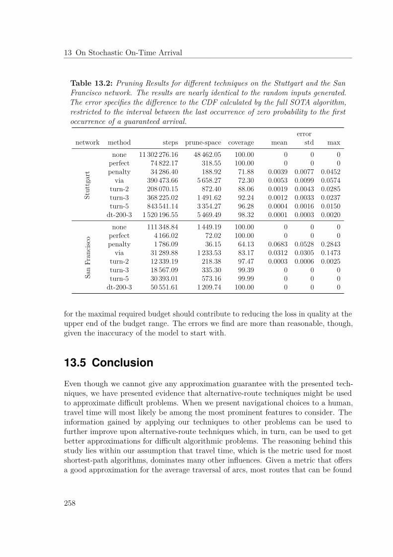
13 On Stochastic On-Time Arrival
Table 13.2: Pruning Results for different techniques on the Stuttgart and the SanFrancisco network. The results are nearly identical to the random inputs generated.The error specifies the difference to the CDF calculated by the full SOTA algorithm,restricted to the interval between the last occurrence of zero probability to the firstoccurrence of a guaranteed arrival.
errornetwork method steps prune-space coverage mean std max
Stut
tgar
t
none 11 302 276.16 48 462.05 100.00 0 0 0perfect 74 822.17 318.55 100.00 0 0 0penalty 34 286.40 188.92 71.88 0.0039 0.0077 0.0452
via 390 473.66 5 658.27 72.30 0.0053 0.0099 0.0574turn-2 208 070.15 872.40 88.06 0.0019 0.0043 0.0285turn-3 368 225.02 1 491.62 92.24 0.0012 0.0033 0.0237turn-5 843 541.14 3 354.27 96.28 0.0004 0.0016 0.0150
dt-200-3 1 520 196.55 5 469.49 98.32 0.0001 0.0003 0.0020
San
Fran
cisc
o
none 111 348.84 1 449.19 100.00 0 0 0perfect 4 166.02 72.02 100.00 0 0 0penalty 1 786.09 36.15 64.13 0.0683 0.0528 0.2843
via 31 289.88 1 233.53 83.17 0.0312 0.0305 0.1473turn-2 12 339.19 218.38 97.47 0.0003 0.0006 0.0025turn-3 18 567.09 335.30 99.39 0 0 0turn-5 30 393.01 573.16 99.99 0 0 0
dt-200-3 50 551.61 1 209.74 100.00 0 0 0
for the maximal required budget should contribute to reducing the loss in quality at theupper end of the budget range. The errors we find are more than reasonable, though,given the inaccuracy of the model to start with.
13.5 Conclusion
Even though we cannot give any approximation guarantee with the presented tech-niques, we have presented evidence that alternative-route techniques might be usedto approximate difficult problems. When we present navigational choices to a human,travel time will most likely be among the most prominent features to consider. Theinformation gained by applying our techniques to other problems can be used tofurther improve upon alternative-route techniques which, in turn, can be used to getbetter approximations for difficult algorithmic problems. The reasoning behind thisstudy lies within our assumption that travel time, which is the metric used for mostshortest-path algorithms, dominates many other influences. Given a metric that offersa good approximation for the average traversal of arcs, most routes that can be found
258

13.5 Conclusion0.
001
0.01
110
0 10 20 30 40 50 60 70 80 90 100
Interpolated Budget (Percentage of [Min,Max])
Abs
olut
e di
ffere
nce
in C
DF
[%]
●●●●●●●●●●●●●●●●●●●●●●●●●●●●●●●●●●●
●●●●●●●●●●●●●●●●●●●●●●●●●●●●●●●●●●●●●●●●●●●●●●●●●●●●●●●●●●●●●●●
●●
●●●●●●●●●●●●●●●●●●●●●●●●●●●●●●●●●●●●●●●●●●●●●●●●●●●●●●●●●●●●●●●●●●●●
●●●●●●●●●●●●●●●●●●●●●●●●●●●●
●●●
●
●
●
penaltyviaδt = 200R32−turn3−turn5−turn
(a) San Francisco
0.00
10.
011
10
0 10 20 30 40 50 60 70 80 90 100
Interpolated Budget (Percentage of [Min,Max])
Abs
olut
e di
ffere
nce
in C
DF
[%]
●●●●●●●●●●●●●●●●●●●●●●●●●●●●●●●●●●●●●●●●●●●●●●●●●●●●●●●●●●●
●●●●●●●●●●●●●●●●●●●●●●●●●●●●●●●●●●●●●●●●
●
●●●●●●●●●●●●●●●●●●●●●●●●●●●●●●●●●●●
●●●●●●●●●●●●●●●●●●●●●
●●●●●●●●●●●
●●●●●●●●●●●●●●●●●●●●●●●●●●●●●●●●
●
●
●
penaltyviaδt = 200R32−turn3−turn5−turn
(b) Stuttgart
Figure 13.6: Error variation in the CDF at the source over the range between theminimal and the maximal required budget.
259
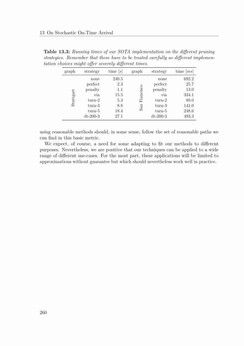
13 On Stochastic On-Time Arrival
Table 13.3: Running times of our SOTA implementation on the different pruningstrategies. Remember that these have to be treated carefully as different implemen-tation choices might offer severely different times.
graph strategy time [s] graph strategy time [ms]St
uttg
art
none 240.5
San
Fran
cisc
o
none 692.2perfect 2.3 perfect 25.7penalty 1.1 penalty 13.0
via 15.5 via 334.1turn-2 5.3 turn-2 89.0turn-3 8.8 turn-3 141.0turn-5 18.4 turn-5 248.6
dt-200-3 27.1 dt-200-3 493.3
using reasonable methods should, in some sense, follow the set of reasonable paths wecan find in this basic metric.
We expect, of course, a need for some adapting to fit our methods to differentpurposes. Nevertheless, we are positive that our techniques can be applied to a widerange of different use-cases. For the most part, these applications will be limited toapproximations without guarantee but which should nevertheless work well in practice.
260
14Chapter 14
Conclusion
A few final thoughts and closing remarks.
Whereas the calculation of shortest paths in road networks is a thoroughly studiedproblem and offers solutions that can answer distance queries within the time requiredfor a few random memory accesses, the same does not hold true for the calculation ofalternative routes. The problem is, in itself, hard to specify as it remains an ambiguoustask. Opposed to a static metric for which we can easily define optimal paths, thequestion of how to define an optimal alternative route is hard to answer, apart froma few rare cases. As long as we cannot find two perfectly disjoint paths of the samelength, the paths most likely become incomparable and offer a full set of Pareto-optimalchoices.
Alternative Route Quality. The propositions of Abraham et al. offer an intuitive setof criteria for the quality of an alternative route. Especially the bounded stretch andlimited sharing present requirements that are, in our view, without a doubt absolutelyjustified. The travel time alone might not be the only reasonable criterion, especially aswe cannot determine it to a perfect accuracy, but one can easily see that it remains animportant part of any travel. The value of the criterion of limited sharing is even moreobvious. Offering a tiny difference on a long journey might constitute a good path onits own, the relevance to a driver is questionable, though. This justifies the requirementof a certain amount of variance very well. The requirement for local optimality is,due to its origin in the via-vertex paradigm, a bit too specialized in our view. Insome regions we can find parallel roads of different types which might each offer apreferable choice for different drivers, but one of them might not offer an optimal pathbetween any two points on it. The considerations purely based on travel-time can alsobe considered problematic when – as it is the case in Berlin – there are some muchfaster roads that might nevertheless be considered undesirable by some. An inner cityhighway might offer far better travel times on average but is associated with a higher
261

14 Conclusion
stress level. In shorter travels, the relative amount of additional time someone mightconsider acceptable to invest can be larger than for long journeys. When driving forten hours, a detour of twenty-five percent in length is a considerable amount of time.Given a journey of ten minutes, one might choose a fifteen-minute one in order to avoidsome uncomfortable driving.
Results. Besides considerations regarding quality, we have presented a wide range oftechniques in this work that offer ways to compute a great variety of different alternativeroute types as well as the possibility of solving other problems and supporting othertasks. As is the case with the basic problem that we studied, it is, in our eyes, impossibleto offer a single solution that presents the best method to compute alternative routes.As the routes themselves, each of the presented approaches offers its own merits and canbe considered viable on its own. Whereas the corridors seem inferior to the techniquesspecifically designed to compute alternative routes, they shine in our experimentalstudy of the stochastic on-time arrival problem. The parallel implementation ofthe bi-criteria shortest-path problem, while too slow for an interactive algorithm oncontinental networks, offers a tool to use in one of the many algorithms that concernthemselves with bi-criteria searches. Our presented data structures that enable thisparallel algorithm are even useful on their own for sets with bulk operations. One of themajor benefits of our algorithms to compute alternative routes is their independence ofthe quality criteria in Definition 5.3. Since in all of our techniques but the bi-criteriasearch we compute graphs that are independent of these criteria, the selection processshould be able to adjust in reasonable ways to other possible criteria one might thinkof. Other techniques are much more sensitive to these criteria and could suffer severelyunder a change of requirements. The considerations we presented offer a good selection,using multiple accepted speed-up techniques that are also used in commercial systems.
Open Questions. Next to further potential optimizations that could bring thepenalty method down to below a hundred milliseconds for all tested queries, some otherquestions remain. The most interesting in our view is not an algorithmic question,though. In our opinion, to improve the quality of alternative routes it is most relevantto understand what constitutes a good alternative route. This would require a thoroughstudy that is beyond the scope of this thesis, however. Nevertheless, we are positivethat the results presented in this thesis offer a good way of calculating alternativeroutes for many possible definitions of quality, as long as the travel time remains acentral component of the quality criteria1.
1Of course we would be able to consider any other metric for our penalty method and all othermetrics that offer a similar hierarchy in a network as travel time does.
262

� Glossary
Symbols
#arc mNumber of arcs in a graph. [10, 14, 18, 23, 54–56]
#vertex nNumber of vertices in a graph. [10, 14, 18–21, 23, 29, 37, 40, 63, 71, 85, 87, 88, 101, 196, 197,245]
k-ary heapA specific implementation of a priority queue, using balanced trees with a branchingfactor of k. [13]
A
algorithm engineeringA branch of algorithmic theory that focuses both on asymptotic guarantees and strongperformance on real-world instances. It is usually described at as cycle of design,analysis, implementation, and experiments. [3, 15, 17, 22, 23, 40]
arc AAn ordered pair (u, v) of vertices. The first vertex (u) is referred to as the origin,the second (v) as the destination of the arc. In our setting, an arc represents a roadsegment between two intersections. [9–22, 24–30, 33–39, 41, 43–46, 48, 50–52, 54–60, 64, 65,68–70, 73, 74, 76, 84–86, 89, 101, 103, 110, 112, 113, 117–125, 127, 129, 133–136, 141, 142, 148–150,152–159, 161–163, 165, 166, 173, 178–182, 185, 192, 194–196, 199–201, 203, 205, 206, 208, 217, 218,222, 226, 235, 245–251, 255, 256, 258, 263–268, 270–273, 318, 320–322]
263

Glossary
B
B-treeA search tree with multiple router keys per node. Its origins stem from databases thattry to minimize block accesses to a HDD. [83, 86, 90, 92–112, 114, 306, 313, 316, 317]
binary heapA specific implementation of a priority queue, footing a a balanced binary tree. Alsogeneralized as k-ary heap. [13, 144]
border arcAn arc whose origin and destination belong two different cells of a partition. [27, 43]
border vertexIn a partition of the vertices of a graph, a border vertex is a vertex that has an adjacentarc whose destination is located in a different cell than its origin. [22, 27, 42, 44, 45, 65,132, 134]
bounded stretch BSCondition for the viability of alternative routes due to Abraham et al.: an alternativeround may not contain segments that are much longer than the best possible distancebetween the endpoints of said segment. [60, 61, 78, 121–123, 142, 164, 172, 178, 180, 185, 199,239, 261, 273, 335]
bucket heapA specific implementation of a priority queue, using buckets in a simplified waycompared to radix heap. [13, 14]
budget TThe longest time available for a journey from a source to a target. [244–254, 256–259]
C
cell CElement of a partition. [22, 26, 27, 41–45, 47, 48, 64, 65, 130–138, 141, 142, 174, 176, 177, 181,195, 264, 311, 321, 322]
cliqueA clique is a (sub-)graph (G (V, A))that contains the arc (u, v) for all u, v ∈ V . [41, 43,44]
contractContraction describes an operation that reduces the size of a graph by reducing thenumber of vertices in a controlled (and reverseable) way. Usually part of a heuristic to
264

Glossary
enable more expensive algorithms to operate on smaller graphs. [28, 29, 33–35, 37, 39, 153,159, 165, 220, 271, 272]
corridor ΓA set of vertices with associated shortest path information directed at a common target.[4, 123, 191–206, 208, 212, 213, 216–227, 229, 232–235, 240, 253, 255–257, 262, 327, 328, 333–336]
cost μSynonym for the value that a metric assigns to an arc. [13, 18, 19, 26, 35, 36, 39, 46, 55, 74,84, 110, 112, 113, 119, 132, 135, 136, 165, 172, 198, 200, 245, 247, 250, 251, 266, 269, 318, 320]
cost bound ΔAn upper bound for the value of μ (a ∈ A) [13, 14, 23]
cost function μSynonym for a metric. [9]
D
degree δ (·)Measure. Describes the number of outgoing (or ingoing) arcs at a vertex. [10, 28, 40, 69,74, 89, 97, 100, 101, 109–111, 133, 196, 197, 199, 217, 218]
destinationThe second vertex of an arc. [9, 22, 24, 45, 152, 161, 218, 263, 264]
diameter DThe length of the longest shortest path within a weighted graph. [11, 41, 71]
distance DThe length of the shortest path between two vertices in a weighted graph. [10–12, 17–19,21, 23–31, 33–35, 37, 38, 41–44, 49, 54–62, 73, 74, 76, 78, 84, 120–125, 127–130, 134, 142–144, 150,152, 154, 157, 158, 162–165, 167, 173–176, 178, 180, 183–185, 192–194, 196–198, 218–223, 226, 235,251, 252, 261, 264, 266, 267, 269–271, 321, 322]
dominateA label dominates another label if it is better or equal in every aspect considered forthe label. [83–87, 89, 90, 107]
F
FIFO propertyIn terms of time-dependent, the FIFO property requires the metrics to assure thatwaiting at a vertex is never beneficial. [16]
265

Glossary
G
goal-directionA paradigm in which a search is augmented with a sense of direction that restrictssearches to reasonable directions. [24–26, 193]
graph GA collection of vertices and arcs. The theoretical concept of a graph is used to describea road network by mapping intersections to vertices and road segments to arcs. [x,5, 9–16, 18–22, 24, 25, 27–30, 33–46, 51, 54–57, 60, 62–64, 68–74, 76, 78, 85, 86, 97, 109–111, 113,115, 117–125, 127–129, 133, 135, 138, 140, 142, 143, 147–167, 171, 173, 177, 178, 180–182, 185, 192,194–197, 199, 203, 205, 206, 208, 212, 218–223, 226, 231, 233, 235, 239, 244–249, 253–255, 262–265,268, 270–272, 306, 307, 309, 310, 322, 326, 327]
H
highway dimension hA measure classifying the minimal size of a hitting set covering all shortest paths. [40,41, 196, 197]
hitting setA hitting set with respect to a collection of sets Si is a set of elements sj such thatSi ∩ sj = ∅ . [40, 41, 266]
L
label �A label is a value or set of values assigned to a vertex. It is usually used as a distance-label and describes the length of a path from a given source to the respective vertex.[13, 14, 17, 18, 20, 25, 73, 74, 83–87, 89, 90, 95–104, 107, 109–114, 265, 266, 269–271]
label-settingA label-setting algorithm is an implementation of the general labeling algorithm. Duringthe execution, a label or vertex is relaxed only once. [18, 86, 107, 110, 113, 246]
leafA leaf is a reference to a special node in a search tree. Leaves are located at the lowestlevel of the tree and has no descendants. [86, 87, 92–96, 98–100, 102–104, 106, 107, 270, 316,317]
length LSummed cost of the arcs of a path [11, 16–20, 34, 40, 41, 49, 50, 52, 55–57, 60, 61, 68, 72, 78,79, 85, 102, 103, 117, 121–123, 125, 157, 162, 175, 177, 178, 180, 181, 184, 185, 187, 196, 205, 219,261, 265, 266, 270]
266

Glossary
level �Hierarchical data structures and algorithms are based on levels. A level in a hierarchydescribes a set of elements that are equal in their height in the hierarchy. [22, 25, 27–29,31, 38, 41–45, 47, 51, 63, 64, 93, 98, 102, 103, 130–141, 147, 150, 152–154, 176, 177, 179, 194, 195,205, 215, 220, 222, 231, 232, 311, 312, 321–323]
LIFOLast in first out principle. The element last added is the first one to be removed. [271]
limited sharing BSCondition for the viability of alternative routes due to Abraham et al.: the alternativeroute is allowed only to share a limited amount of distance traveled with the originalshortest path. [59–61, 63, 76, 78, 122–124, 167, 174, 175, 178, 180, 185, 233, 261, 275, 305, 335]
local optimality LOCondition for the viability of alternative routes due to Abraham et al.: every sufficientlyshort segment of an alternative route has to be a shortest path. [60, 61, 78, 122, 133, 142,148, 167, 185, 199, 239, 247, 255, 261, 275, 335]
M
metric μA metric is a function μ : A �→ R . Typical examples are travel time, distance, oreconomic cost required to traverse an arc. [9–11, 13, 16–21, 26–29, 34, 35, 41–43, 46, 49, 50,52, 54, 56, 58, 59, 73, 74, 83–86, 103, 110, 114, 118–122, 124, 127, 128, 142, 152, 163, 172, 173, 192,196, 197, 231, 243, 245, 246, 248–251, 253, 257, 258, 260–262, 265, 267–269, 271, 272, 322]
microcodeOperations describing the process of constructing a CH under the assumptions of allshortcuts to be necessary. [43, 44, 47, 48, 134]
N
nodeA node is the basic element that makes up a search tree. [86–88, 92–97, 99, 100, 102, 264,266, 269, 270]
O
Open-MPA multi-threading library. [176]
originThe first vertex of an arc. [9, 11, 38, 45, 152, 161, 218, 263, 264, 271]
267

Glossary
overlay graphAn overlay to a graph (G (V, A)) is a graph itself, defined on a subset of the vertices V .For arcs, the overlay-graph may contain a combination of arcs from A as well as newarcs. The concept of overlay-graphs is usually used to characterize a larger graph byrepresenting essential parts of it using a smaller graph. [10, 27–29, 33–35]
P
Pareto dominanceA solution to a problem dominates another solution if it is better or equal to thedominated solution in every aspect of the criteria. [16]
Pareto-optimalIn a multi-criteria setting, a Pareto-optimal solution describes a solution to which noother solution exists that is better in every aspect of the desired criteria. [ix, 16, 52, 72,73, 83–91, 95–98, 100–104, 107–109, 111–115, 261, 306, 313, 318–320]
partition PCollection of subsets Si to a set S with ⋃
i Si = S ∧ Si ∩ Sj = ∅. [21, 22, 26–28, 41–45, 64,65, 133, 134, 136, 142, 144, 197, 264, 309, 311]
path PA series of vertices of a graph, connected by arcs. [11, 15–20, 23–25, 29, 30, 33–39, 44, 45,49–57, 59–61, 63, 65, 69, 72, 73, 77, 78, 83, 87, 88, 102, 103, 117–125, 127, 129–131, 133–137, 141, 142,147, 148, 150, 152, 155, 157–159, 162–165, 167, 172–180, 185, 191, 192, 194–198, 202, 203, 208, 212,217, 219, 223, 225, 231–233, 239, 240, 243–247, 251–256, 260, 261, 266, 270, 272, 322]
planarPlanar is a possible property of a graph. A planar graph can be drawn on a 2D-surfacewithout any crossings in the arcs. [9, 27, 40, 73]
plateauA plateau describes a shared segment between two shortest paths. [52, 53, 55, 57–59, 62,133, 148, 149, 152, 154–158, 162, 165, 232, 233, 235, 239, 240, 255]
potential πA potential describes a built-up of energy. For our purposes, we view the potential as alower bound for the length of a shortest path with respect to a given metric. [26, 58, 84]
priority queue QAbstract data structure that enables efficient retrieval of elements ordered by somepriority. [ix, 12–14, 18, 19, 23–26, 36, 38, 85–89, 94, 95, 97, 98, 100, 101, 103, 104, 107–109, 112–114,151, 197, 249, 263, 264, 269, 306, 313]
268

Glossary
pruneA process in which unnecessary overhead in a search is detected and the respectivecomputations are eliminated before they are executed. [25, 63, 135, 147, 151, 159, 164, 166,169, 193–195, 219–221, 225, 250, 254–257, 270]
R
radix heapA specific implementation of a priority queue, utilizing properties of integer representa-tion, maximum arc weights, and a bucket structure. [14, 144,264]
reach rA centrality measure on vertices. The reach of a vertex v is the maximum over theminimal distances to the source/target (D (s, v)/D (v, t)) of any potential shortest paththat contains v . [28, 62–64, 179, 246]
reachedA vertex that has been assigned a tentative distance label. The label is not known tobe final. [18, 19, 35, 103]
registerA register describes the typical access form on which the CPU operates. Data has tobe transferred from RAM to a register before the CPU can perform operations on it.[92]
relaxationIn the context of shortest path algorithms, the relaxation of an arc represents thecreation of new tentative distance labels by extending a path ending at a given vertexby and additional arc, adding the cost (defined by the metric) of the respective arc tothe label. In hierarchical speed-up techniques, the relaxation weakens the hierarchyaccording to some criteria. [17, 18, 48, 64, 86, 101, 103, 113, 147–150, 154, 171, 198, 232, 250,266]
robust �The degree to what a corridor can be used to correct for incorrect driving behavior.[192–194, 196, 200, 201, 203, 226]
rootThe root of a search tree is the topmost node. It is the only node that is not adescendant to any other node. [86–88, 93, 94, 98, 270]
269

Glossary
S
search space SThe search space with respect to a pruning (or speed-up) technique describes the subsetof vertices of a graph that is considered during the pruned search. [25, 36, 37, 40, 46, 58,131, 149–152, 161, 162, 164, 165, 194, 218–221, 223, 256]
search treeA search tree is an ordered collection of interconnected nodes used to store elementsthat are identified by a comparable key. Every node splits its descendants into partsbased on a set of router keys, distributing the stored elements into subtrees. Usuallysearch trees are kept in balance, allowing to locate an arbitrary key within logarithmictime by following the router keys from the topmost node (the root) to a leaf. The mostcommon search tree uses a single router key per node, splitting the elements in half. Itis referred to as binary search tree. [86–90, 92–95, 97, 100, 102, 104, 264, 266, 267, 269]
segment SA continuous subsequence of vertices along a path. [4, 79, 117, 122–124, 152, 155, 157–159,166, 171–181, 184, 185, 189, 240, 255]
separator SA separator to a set S of connected elements describes a set of elements that fragmentsS into disjoint parts. [21, 22, 27, 40, 41]
settledA vertex with final distance label (correct shortest path distance) in an implementationof Dijkstra’s algorithm or any implementation following the general procedure ofDijkstra’s algorithm. [18, 19, 25, 36, 71, 85, 103, 198, 217]
shortcutArtificial arc in a graph that represents an entire path (not necessarily a shortest path)within another graph. [27–29, 33–37, 39, 40, 43–46, 51, 63, 132, 147–149, 152–161, 165, 166, 196,221–223, 267, 271, 272]
shortest path Πpath of minimal length between two vertices in a weighted graph. [1, 3, 10–12, 14–21, 23,25, 26, 28–30, 33–38, 40, 41, 44–46, 49–57, 59–64, 68, 71, 72, 74, 76, 78, 83–85, 109, 112, 114, 115,117, 120–122, 129–132, 135, 136, 138, 141, 144, 147–149, 151, 152, 154, 155, 162, 165, 167, 172, 173,175–178, 180, 181, 187, 189, 191–198, 201, 203, 205–207, 209–211, 217–223, 225, 228, 239, 244, 252,253, 256, 258, 261, 262, 265–272, 276, 305, 306, 318–320, 329–332]
simpleProperty of a path within a graph. A simple path does not contain any vertex twice.[20]
270

Glossary
source sThe origin of a shortest path query. [11, 15–20, 23–28, 30, 31, 34–38, 44, 45, 51–53, 56, 57,59–63, 65, 70, 71, 73, 85, 103, 119–124, 131, 132, 135–138, 142, 147, 149–152, 154, 156, 162, 163, 175,176, 178, 180, 183–185, 191–197, 199, 200, 202, 203, 217–219, 221, 222, 225, 228, 233, 243, 245, 248,249, 251, 252, 254–257, 259, 264, 266, 269, 272, 321, 322]
speed-upRelation between experienced running time of an algorithm and a comparative baselinealgorithm. [1, 20, 22, 23, 25, 27–30, 33, 39, 49, 51–53, 59, 62, 64, 65, 105, 110, 112–114, 117, 138,147, 148, 167, 193, 218, 262, 269–271, 306, 318–320]
stackA container data structure that operates on the LIFO principle. [217]
T
target tThe destination of a shortest path query. [11, 16, 18–20, 23–28, 30, 31, 34–36, 44, 45, 51–53,56, 57, 59–63, 65, 70, 71, 119–124, 131, 132, 135–138, 142, 147, 149–152, 156, 162, 163, 175, 176, 178,180, 183–185, 192–200, 202, 203, 217–219, 221, 222, 225, 228, 233, 243, 245, 247–249, 251, 252, 254,255, 264, 265, 269, 272, 321, 322]
time-dependentTime-Dependency in routing considers a series of metrics. The metrics are referencedto by the expected arrival time at the origin of the arc. [16, 17, 39, 53, 55, 74, 76, 243, 244,265]
U
undirectedProperty of a graph. A graph is undirected if ∀a = (u, v) ∈ A : (v, u) ∈ A . [196]
unpackReverse process of shortcut creation or contraction. Used to extract the actual shortestpaths from a speed-up-technique based on shortcuts. [37, 51, 153–159, 161]
unreachedA vertex that has not been assigned a tentative distance label less than ∞. [18, 19]
unweightedProperty of a graph. A graph is called unweighted if no metric has been defined on itsarcs. [9]
271

Glossary
V
vertex VBasic construction element of a graph. In route planning vertices usually represents anintersection. [4, 9–11, 14–30, 33–38, 40–42, 44, 45, 48, 50–52, 54–56, 58–65, 68–71,73, 74, 76, 84–89, 96, 97, 100–103, 107, 109, 110, 117, 118, 120–123, 130, 132–134, 147–163, 165–167,171–181, 185, 189, 192–201, 203, 208, 212, 217–223, 226, 228, 231–233, 235, 240, 245–251, 253–257,261, 263–272, 322, 335]
via-vertex vIntermediate destination on a trip that, in combination with source and target fullydescribes an alternative route via the shortest paths Πs,v concatenated with Πv,t. [4, 52,58–60, 62–65, 147–149, 165, 167, 171–173, 180, 189, 226, 231, 232, 235, 240, 256, 257, 261, 306, 307,335]
W
weight μSynonym for the value that a metric assigns to an arc. [43, 56, 103, 246]
weightedProperty of a graph. A graph is called weighted if a metric has been defined on itsarcs. [9–11, 14–16, 19–21, 34, 35, 41, 56, 85, 150, 265, 270]
witnessIn the context of contraction, a witness to a potential shortcut is a path that is shorterthen the potential shortcut and thus proves the shortcut to be unnecessary. [29, 33–35,43, 162]
272

� Acronyms
Symbols
CRP-∞Customizeable Route Planning with Infinite Penalization [171, 176, 180, 181, 183, 186,232–235, 239, 240, 338]
CRP-πCustomizeable Route Planning with Penalization [144, 171–173, 176, 180–186, 189, 232–235,239, 240, 309, 312, 321, 325, 338]
A
ALTA* Landmarks Triangle Inequality [26, 58, 117–119, 193, 194]
ArcFlagsArc-Flags [148, 193–195, 246]
B
BFSbreadth-first search [150]
BSbounded stretch [60, 61, 76, 78, 79, 121–124, 133, 142, 164, 172, 178, 180, 185, 199, 233, 239, 261,264, 267, 305, 335]
C
CCHCustomizeable Contraction Hierarchies [118]
273

Acronyms
CDFCumulative Distribution Function [247–249, 251, 254–259]
CHContraction Hierarchy [29, 30, 33–41, 43–46, 51, 58, 63–65, 118, 135, 148–154, 159, 161, 164, 167,171, 172, 181, 185, 189, 192, 194, 219, 222, 223, 225, 228, 231, 232, 240, 255, 267, 306]
CPUCentral Processing Unit [29, 37, 46–48, 92, 107, 181, 185, 269, 322, 323]
CRPCustomizeable Route Planning [27, 33, 41–47, 50, 118, 119, 129–137, 139, 140, 144, 171–173,176, 179–186, 189, 194, 196, 231–235, 239, 240, 273, 307, 309, 312, 321, 322, 325, 338]
D
DAGDirected Acyclic Graph [50, 150, 154, 192, 198, 253, 254]
DFSdepth-first search [14, 15, 162, 164, 199]
DFTDiscrete Fourier-Transformation [250]
F
FFTFast Fourier-Transformation [246, 249, 250]
G
GPGPUGeneral Purpose Graphics Processing Unit [38, 46–48, 300, 307]
GPSGlobal Positioning System [68, 75, 201]
H
HHHighway Hierarchies [28, 29]
274

Acronyms
HiDARHierarchy Decomposition for Alternative Routes [149, 151, 152, 154, 158, 162, 164–167, 169,170, 194, 196, 232–235, 239, 240, 255, 337]
HNRHighway Node Routing [28, 29, 40, 58, 118]
I
I/OInput/Output [94]
IDIdentification [96, 156, 158, 161]
L
LOlocal optimality [60–62, 76, 78, 122, 129, 133, 142, 148, 167, 185, 199, 239, 247, 255, 261, 267, 305,335]
LSlimited sharing [60, 61, 124]
P
PEMParallel External Memory [94]
PHASTParallel Hardware Accelerated Shortest Path Trees [30, 37, 38, 148–151, 218, 220, 222]
R
RAMRandom Access Memory [92, 269]
RPHASTRestricted PHAST [149–152]
S
SASuccessive Approximation [245, 247]
275

Acronyms
SCCStrongly Connected Component [14, 69]
SOTAstochastic on-time arrival problem [243–258, 260, 262, 307]
SPOTARshortest path with on-time arrival reliability [244–246, 251, 252]
SPPSingle Source Shortest Path Problem [16–18, 22, 23, 49, 70, 84, 85, 243]
STDStandard Template Library [105, 176]
T
TLBTransaction Look-aside Buffer [94]
TNRTransit Node Routing [30, 31, 41]
TTFtravel time function [16, 17, 53, 55]
U
UDGUnit Disc Graph [74]
W
WLANWireless Local Area Network [191]
Z
ZDCZero-Delay Convolution [249, 250]
276

� Bibliography
[ADF+11] Ittai Abraham, Daniel Delling, Amos Fiat, Andrew V. Goldberg, andRenato F. Werneck. VC-dimension and shortest path algorithms. InInternational Colloquium on Automata, Languages, and Programming(ICALP), volume 6755 of Lecture Notes in Computer Science, pages690–699. Springer, 2011. [see pages 30 and 40]
[ADF+12] Ittai Abraham, Daniel Delling, Amos Fiat, Andrew V. Goldberg, and Re-nato Fonseca F. Werneck. HLDB: Location-based services in databases.In ACM SIGSPATIAL International Conference on Advances in Geo-graphic Information Systems (GIS), pages 339–348, 2012. [see page 30]
[ADF+13] Ittai Abraham, Daniel Delling, Amos Fiat, Andrew V. Goldberg, andRenato F. Werneck. Highway dimension and provably efficient shortestpath algorithms. Technical Report MSR-TR-2013-91, Microsoft Re-search, 2013. [see pages 40and 41]
[ADGW11] Ittai Abraham, Daniel Delling, Andrew V. Goldberg, and Renato F.Werneck. A hub-based labeling algorithm for shortest paths on roadnetworks. In International Symposium on Experimental Algorithms(SEA), volume 6630 of Lecture Notes in Computer Science, pages 230–241. Springer, 2011. [see pages 30and 92]
[ADGW12] Ittai Abraham, Daniel Delling, Andrew V. Goldberg, and Renato F.Werneck. Hierarchical hub labelings for shortest paths. In ExperimentalAlgorithms, volume 7501 of Lecture Notes in Computer Science, pages24–35. Springer, 2012. [see page 30]
277

Bibliography
[ADGW13] Ittai Abraham, Daniel Delling, Andrew V. Goldberg, and Renato F.Werneck. Alternative routes in road networks. ACM Journal of Experi-mental Algorithms, 18(1):1–17, 2013. [see pages 52, 59, 61, 62, 64, 65, 68,76, 78, 147, 149, 164, 167, 171, 175, 180, 232, and 233]
[AFGW10] Ittai Abraham, Amos Fiat, Andrew V. Goldberg, and Renato F. Wer-neck. Highway dimension, shortest paths, and provably efficient algo-rithms. In ACM-SIAM Symposium on Discrete Algorithms (SODA),pages 782–793. Society for Industrial and Applied Mathematics (SIAM),2010. [see pages 40, 41, and 62]
[ALS13] Julian Arz, Dennis Luxen, and Peter Sanders. Transit node routingreconsidered. In International Symposium on Experimental Algorithms(SEA), pages 55–66, 2013. [see page 30]
[AMOT90] Ravindra K. Ahuja, Kurt Mehlhorn, James Orlin, and Robert E. Tarjan.Faster algorithms for the shortest path problem. Journal of the ACM,37(2):213–223, April 1990. [see page 14]
[AV03] Lars Arge and Jeffrey Scott Vitter. Optimal external memory intervalmanagement. SIAM Journal on Computing (SICOMP), 32(6):1488–1508, 2003. [see pages 91, 93, 94,and 95]
[BABDR84] M Ben-Akiva, MJ Bergman, Andrew J Daly, and Rohit Ramaswamy.Modeling inter-urban route choice behaviour. In International Sympo-sium on Transportation and Traffic Theory, pages 299–330. VNU Press,1984. [see pages 49 and 50]
[Bat14] Gernod Veit Batz. Time-Dependent Route Planning with ContractionHierarchies. Phd thesis, Karlsruhe Institute of Technology, Departmentof Informatics, 2014. [see pages 16, 39, 53, and 243]
[BCK+10] Reinhard Bauer, Tobias Columbus, Bastian Katz, Marcus Krug, andDorothea Wagner. Preprocessing speed-up techniques is hard. InAlgorithms and Complexity (CIAC), volume 6078 of Lecture Notes inComputer Science, pages 359–370. Springer, 2010. [see page 34]
[BCRW13] Reinhard Bauer, Tobias Columbus, Ignaz Rutter, and Dorothea Wagner.Search-space size in contraction hierarchies. In International Colloquiumon Automata, Languages, and Programming (ICALP), Lecture Notesin Computer Science, pages 93–104, 2013. [see pages 39 and 43]
278

Bibliography
[BDFC00] Michael A. Bender, Erik D. Demaine, and Martin Farach-Colton. Cache-oblivious B-trees. In Foundations of Computer Science, pages 399–409.IEEE Computer Society, 2000. [see page 93]
[BDG+15] Hannah Bast, Daniel Delling, Andrew V. Goldberg, Matthias Müller-Hannemann, Thomas Pajor, Peter Sanders, Dorothea Wagner, andRenato F. Werneck. Route planning in transportation networks. Com-puting Research ReposFitory, abs/1504.05140, 2015. [see pages 25, 29,30, and 68]
[BDGS11] Roland Bader, Jonathan Dees, Robert Geisberger, and Peter Sanders.Alternative route graphs in road networks. In International ICST Con-ference on Theory and Practice of Algorithms in (Computer) Systems(TAPAS), volume 6595 of Lecture Notes in Computer Science, pages21–32. Springer, 2011. [see pages 50, 51, 52, 54, 55, 57, 58, 59, 76, 77, 115,117, 119, 120, 121, 125, 128, 144, 148, 167, 181, and 233]
[BDMR96] Armin Bäumker, Wolfgang Dittrich, Friedhelm Meyer auf der Heide, andIngo Rieping. Realistic parallel algorithms: Priority queue operationsand selection for the BSP model. In Parallel Processing (EuroPar),Lecture Notes in Computer Science, pages 369–376. Springer, 1996.
[see page 95]
[Bel58] Richard Bellman. On a routing problem. Quarterly of Applied Mathe-matics, 16:87–90, 1958. [see pages 15and 19]
[BFGK05] Michael A. Bender, Jeremy T. Fineman, Seth Gilbert, and Bradley C.Kuszmaul. Concurrent cache-oblivious B-trees. In Symposium onParallelism in Algorithms and Architectures (SPAA), pages 228–237.Association for Computing Machinery (ACM), 2005. [see page 93]
[BFM+07] Holger Bast, Stefan Funke, Domagoj Matijevic, Peter Sanders, andDominik Schultes. In transit to constant time shortest-path queriesin road networks. In Workshop on Algorithm Engineering and Exper-iments (ALENEX). Society for Industrial and Applied Mathematics(SIAM), Society for Industrial and Applied Mathematics (SIAM), 2007.
[see page 30]
[BFM09] Holger Bast, Stefan Funke, and Domagoj Matijevic. Ultrafast shortest-path queries via transit nodes. The Shortest Path Problem: NinthDIMACS Implementation Challenge, 74:175–192, 2009. [see pages 30and 68]
279

Bibliography
[BFSS07] Holger Bast, Stefan Funke, Peter Sanders, and Dominik Schultes. Fastrouting in road networks with transit nodes. Science, 316(5824), 2007.
[see pages 30 and 41]
[BGL+12] Gernot V. Batz, Robert Geisberger, Dennis Luxen, Peter Sanders, andRoman Zubkov. Efficient route compression for hybrid route planning.In Mediterranean Conference on Algorithms (MedAlg’12), volume 7659of Lecture Notes in Computer Science, pages 93–107. Springer, 2012.
[see page 53]
[BGSV13] Gernot V. Batz, Robert Geisberger, Peter Sanders, and ChristianVetter. Minimum time-dependent travel times with contraction hierar-chies. ACM Journal of Experimental Algorithms, 18(1.4):1–43, 2013.
[see page 53]
[BK60] Richard Bellman and Robert Kalaba. On k-th best policies. Journal ofthe Society for Industrial & Applied Mathematics, 8(4):582–588, 1960.
[see page 51]
[BKMW10] Reinhard Bauer, Marcus Krug, Sascha Meinert, and Dorothea Wagner.Synthetic road networks. In Algorithmik Aspects of Information andManagement (AAIM), Lecture Notes in Computer Science, pages 46–57.Springer, 2010. [see page 41]
[BM72] R Bayer and EM McCreight. Organization and maintenance of largeordered indexes. Acta Informatica, 1(3):173–189, 1972. [see page 92]
[BM02] Rudolf Bayer and Edward McCreight. Organization and maintenanceof large ordered indexes. Springer, 2002. [see page 92]
[BMS+13] Aydin Buluç, Henning Meyerhenke, Ilya Safro, Peter Sanders, andChristian Schulz. Recent advances in graph partitioning. ComputingResearch ReposFitory, abs/1311.3144, 2013. [see page 22]
[Bro99] Gerth Stølting Brodal. Priority queues on parallel machines. ParallelComputing, 25(8), 1999. [see page 95]
[Cam05] Cambridge Vehicle Information Tech. Ltd. Choice routing,2005. http://camvit.com/camvit-technical-english/Camvit-Choice-Routing-Explanation-english.pdf. Accessed: 2014-03-28.
[see pages 52, 57, 62, and 148]
[CBB07] Yanyan Chen, Michael G. H. Bell, and Klaus Bogenberger. Reliablepretrip multipath planning and dynamic adaptation for a centralized
280

Bibliography
road navigation system. IEEE Transactions on Intelligent Transporta-tion Systems (ITSC), 8(1):14–20, 2007. [see pages 55and 244]
[CBWB06] Yanyan Chen, Michael GH Bell, Dongzhu Wang, and Klaus Bogenberger.Risk-averse time-dependent route guidance by constrained dynamic A*search in decentralized system architecture. Transportation ResearchRecord: Journal of the Transportation Research Board, 1944(1):51–57,2006. [see page 244]
[CGG+95] Yi-Jen Chiang, Michael T Goodrich, Edward F Grove, Roberto Tamas-sia, Darren Erik Vengroff, and Jeffrey Scott Vitter. External-memorygraph algorithms. In ACM-SIAM Symposium on Discrete Algorithms(SODA), pages 139–149. Society for Industrial and Applied Mathemat-ics (SIAM), Society for Industrial and Applied Mathematics (SIAM),1995. [see page 38]
[CGM01] Shimin Chen, Phillip B. Gibbons, and Todd C. Mowry. Improvingindex performance through prefetching. In ACM SIGMOD Symposiumon Principles of Database Systems (PODS), pages 235–246. Associationfor Computing Machinery (ACM), 2001. [see pages 93 and 94]
[CGS97] Boris V. Cherkassky, Andrew V. Goldberg, and Craig Silverstein. Buck-ets, heaps, lists, and monotone priority queues. In ACM-SIAM Sympo-sium on Discrete Algorithms (SODA), pages 83–92. Society for Indus-trial and Applied Mathematics (SIAM), 1997. [see page 14]
[CH94] Danny Z. Chen and Xiaobo Hu. Fast and efficient operations onparallel priority queues. In International Symposium on Algorithmsand Computation (ISAAC), Lecture Notes in Computer Science, pages279–287. Springer, 1994. [see page 95]
[CHL99] Trishul M. Chilimbi, Mark D. Hill, and James R. Larus. Cache-consciousstructure layout. In ACM SIGPLAN Programming Language Designand Implementation (PLDI), pages 1–12. Association for ComputingMachinery (ACM), 1999. [see page 93]
[Cho59] Noam Chomsky. On certain formal properties of grammars. Informationand Control, 2(2):137–167, 1959. [see page 152]
[Cor14] NVIDIA Corporation. CUDA C Programming Guide. NVIDIA Corpo-ration, 2014. http://docs.nvidia.com/cuda/pdf/CUDA_C_Programming_Guide.pdf. [see page 47]
281

Bibliography
[CYGW07] Kun Chen, Lei Yu, Jifu Guo, and Huimin Wen. Characteristics analysisof road network reliability in beijing based on the data logs from taxis.In Transportation Research Board 86th Annual Meeting, number 07-1420in TRB Annual Meeting Compendium, 2007. [see page 74]
[Dan62] George B. Dantzig. Linear Programming and Extensions. PrincetonUniversity Press, 1962. [see page 23]
[DBGO14] Andrew Alan Davidson, Sean Baxter, Michael Garland, and John DOwens. Work-efficient parallel GPU methods for single-source shortestpaths. In International Parallel and Distributed Processing Symposium(IPDPS), volume 28. IEEE Computer Society, 2014. [see page 47]
[DBKS10] Ugur Demiryurek, Farnoush Banaei-Kashani, and Cyrus Shahabi. Acase for time-dependent shortest path computation in spatial networks.In ACM SIGSPATIAL International Conference on Advances in Ge-ographic Information Systems (GIS), pages 474–477. Association forComputing Machinery (ACM), 2010. [see page 244]
[DDF14] Gianlorenzo D’Angelo, Mattia D’Emidio, and Daniele Frigioni. Fullydynamic update of arc-flags. Networks, 2014. Accepted for publication.
[see page 118]
[DDFV12] Gianlorenzo D’Angelo, Mattia D’Emidio, Daniele Frigioni, and CamilloVitale. Fully dynamic maintenance of arc-flags in road networks. InInternational Symposium on Experimental Algorithms (SEA), volume7276 of Lecture Notes in Computer Science, pages 135–147. Springer,2012. [see pages 58 and 118]
[DDP+13] Daniel Delling, Julian Dibbelt, Thomas Pajor, Dorothea Wagner, andRenato F. Werneck. Computing multimodal journeys in practice. InInternational Symposium on Experimental Algorithms (SEA), LectureNotes in Computer Science, pages 260–271. Springer, 2013. [see pages 83and 114]
[Dea10] Brian C Dean. Speeding up stochastic dynamic programming with zero-delay convolution. Algorithmic Operations Research, 5(2):Pages–96,2010. [see page 249]
[DF79] Eric V. Denardo and Bennett L. Fox. Shortest-route methods: 1.reaching, pruning, and buckets. Operations Research, 27(1):pp. 161–186, 1979. [see page 13]
[DFV11] Gianlorenzo D’Angelo, Daniele Frigioni, and Camillo Vitale. Dynamicarc-flags in road networks. In International Symposium on Experimental
282

Bibliography
Algorithms (SEA), volume 6630 of Lecture Notes in Computer Science,pages 88–99. Springer, 2011. [see pages 58 and 118]
[DGJ09] Camil Demetrescu, Andrew V. Goldberg, and David S. Johnson, editors.The Shortest Path Problem: Ninth DIMACS Implementation Challenge,volume 74 of DIMACS Book Series. American Mathematical Society(AMS), 2009. [see page 23]
[DGNW13] Daniel Delling, Andrew V. Goldberg, Andreas Nowatzyk, and Renato F.Werneck. PHAST: Hardware-accelerated shortest path trees. Journal ofParallel and Distributed Computing, 73(7):940–952, 2013. [see pages 27,29, 37, 92, 148, 149, and 220]
[DGPW11] Daniel Delling, Andrew V. Goldberg, Thomas Pajor, and Renato F.Werneck. Customizable route planning. In International Symposiumon Experimental Algorithms (SEA), volume 6630 of Lecture Notes inComputer Science, pages 376–387. Springer, 2011. [see pages 27, 41, 45,129, and 133]
[DGPW13] Daniel Delling, Andrew V. Goldberg, Thomas Pajor, and Renato F.Werneck. Customizable route planning in road networks, 2013.Preprint at http://research.microsoft.com/pubs/198358/crp_web_130724.pdf. Accessed: 2014-03-28. [see pages 27, 41, 45, 68, 125,and 129]
[DGRW11] Daniel Delling, Andrew V. Goldberg, Ilya Razenshteyn, and Renato F.Werneck. Graph partitioning with natural cuts. In InternationalParallel and Distributed Processing Symposium (IPDPS), pages 1135–1146. IEEE Computer Society, 2011. [see pages 27, 40, 41,and 133]
[DGW11] Daniel Delling, Andrew V. Goldberg, and Renato Fonseca F. Werneck.Faster batched shortest paths in road networks. In Workshop onAlgorithmic Approaches for Transportation Modelling, Optimization,and Systems (ATMOS), volume 20 of OpenAccess Series in Informatics(OASICS), pages 52–63, 2011. [see pages 149, 150, 220, and 222]
[DGW13] Daniel Delling, Andrew V. Goldberg, and Renato F. Werneck. Hub labelcompression. In International Symposium on Experimental Algorithms(SEA), pages 18–29, 2013. [see page 30]
[DHM+09] Daniel Delling, Martin Holzer, Kirill Müller, Frank Schulz, and DorotheaWagner. High-performance multi-level routing. In The Shortest PathProblem: Ninth DIMACS Implementation Challenge, volume 74 of
283

Bibliography
DIMACS Book Series, pages 73–92. American Mathematical Society(AMS), 2009. [see page 27]
[Dij59] Edsger W. Dijkstra. A note on two problems in connexion with graphs.Numerische Mathematik, 1(1):269–271, 1959. [see pages 15, 18, and 23]
[DKLW12] Daniel Delling, Moritz Kobitzsch, Dennis Luxen, and Renato F. Wer-neck. Robust mobile route planning with limited connectivity. InMeeting on Algorithm Engineering and Experiments (ALENEX), pages150–159. Society for Industrial and Applied Mathematics (SIAM), 2012.
[see pages 191 and 192]
[DKW14] Daniel Delling, Moritz Kobitzsch, and Renato F. Werneck. Customizingdriving directions with GPUs. In Parallel Processing (EuroPar), LectureNotes in Computer Science. Springer, 2014. [see page 46]
[dlBPA93] Tomas de la Barra, B Perez, and J Anez. Multidimensional path searchand assignment. In PTRC Summer Annual Meeting (SAM), 1993.
[see pages 51, 55, and 56]
[DP84] Narsingh Deo and Chi-Yin Pang. Shortest-path algorithms: Taxonomyand annotation. Computer Networks, 14(2):275–323, 1984. [see page 11]
[DP92] Narsingh Deo and Sushil K. Prasad. Parallel heap: An optimal parallelpriority queue. The Journal of Supercomputing, 6(1):87–98, 1992.
[see page 95]
[DSW14] Julian Dibbelt, Ben Strasser, and Dorothea Wagner. Customizablecontraction hierarchies. In Experimental Algorithms, volume 8504 ofLecture Notes in Computer Science, pages 271–282. Springer, 2014.
[see pages 46, 51, and 58]
[DW07] Daniel Delling and Dorothea Wagner. Landmark-based routing indynamic graphs. In Experimental Algorithms, volume 4525 of LectureNotes in Computer Science, pages 52–65. Springer, 2007. [see page 117]
[DW09] Daniel Delling and Dorothea Wagner. Pareto paths with SHARC. InInternational Symposium on Experimental Algorithms (SEA), LectureNotes in Computer Science, pages 125–136. Springer, 2009. [see page 52]
[DW13] Daniel Delling and Renato F. Werneck. Faster customization of roadnetworks. In International Symposium on Experimental Algorithms(SEA), volume 7933 of Lecture Notes in Computer Science, pages 30–42.Springer, 2013. [see pages 43, 44, 47, 129, and 134]
284
Bibliography
[Edm70] Jack Edmonds. Exponential growth of the simplex method for shortestpath problems. manuscript [University of Waterloo, Waterloo, Ontario],1970. [see page 18]
[EG08] David Eppstein and Michael T Goodrich. Studying (non-planar) roadnetworks through an algorithmic lens. In ACM SIGSPATIAL Inter-national Conference on Advances in Geographic Information Systems(GIS), page 16. Association for Computing Machinery (ACM), Associa-tion for Computing Machinery (ACM), 2008. [see pages 27and 40]
[EKS14] Stephan Erb, Moritz Kobitzsch, and Peter Sanders. Parallel bi-objectiveshortest paths using weight-balanced B-trees with bulk updates. InInternational Symposium on Experimental Algorithms (SEA), volume8504 of Lecture Notes in Computer Science, pages 111–122. Springer,2014. [see pages 91 and 107]
[Epp94] David Eppstein. Finding the k shortest paths. In Foundations ofComputer Science, pages 154–165. IEEE Computer Society, 1994.
[see page 50]
[Epp98] David Eppstein. Finding the k shortest paths. SIAM Journal onComputing (SICOMP), 28(2):652–673, 1998. [see page 50]
[EPV11] Alexandros Efentakis, Dieter Pfoser, and Agnès Voisard. Efficientdata management in support of shortest-path computation. In ACMSIGSPATIAL International Workshop on Computational Transporta-tion Science (CTS), pages 28–33. Association for Computing Machinery(ACM), 2011. [see page 28]
[Erb13] Stephan Erb. Engineering parallel bi-criteria shortest path search.Master’s thesis, Karlsruhe Institute of Technology, Department ofInformatics, 2013. [not cited]
[Flo62] Robert W. Floyd. Algorithm 97: Shortest path. Communications ofthe ACM, 5(6):345, 1962. [see page 21]
[FN06] Yueyue Fan and Yu Nie. Optimal routing for maximizing the traveltime reliability. NSpEc, 6(3-4):333–344, 2006. [see pages 245 and 247]
[For56] Lester R. Ford. Network flow theory. Technical Report Report P-923,The Rand Corporation, 1956. [see pages 15, 17, and 19]
[FS07] Leonor Frias and Johannes Singler. Parallelization of bulk operationsfor STL dictionaries. In Parallel Processing (EuroPar), Lecture Notes
285

Bibliography
in Computer Science, pages 49–58. Springer, 2007. [see pages 90, 97,102, 103, 104, and 105]
[FSR06] L. Fu, D. Sun, and L. R. Rilett. Heuristic shortest path algorithms fortransportation applications: State of the art. Computers & OperationsResearch, 33(11), 2006. [see page 28]
[FW56] Marguerite Frank and Philip Wolfe. An algorithm for quadratic pro-gramming. Naval research logistics quarterly, 3(1-2):95–110, 1956.
[see page 51]
[Gei14] R. Geisberger. Alternate directions in hierarchical road networks,September 2 2014. US Patent 8,824,337. [see pages 64 and 147]
[GH05] Andrew V. Goldberg and Chris Harrelson. Computing the shortestpath: A* search meets graph theory. In ACM-SIAM Symposium onDiscrete Algorithms (SODA), pages 156–165. Society for Industrial andApplied Mathematics (SIAM), 2005. [see page 26]
[GJ79] Michael Randolph Garey and David Stifler Johnson. Computers andIntractability. Freeman and Company, 1979. [see page 16]
[GKS10] Robert Geisberger, Moritz Kobitzsch, and Peter Sanders. Route plan-ning with flexible objective functions. In Workshop on AlgorithmEngineering and Experiments (ALENEX), pages 124–137. Society forIndustrial and Applied Mathematics (SIAM), 2010. [see page 52]
[GKW09] Andrew V. Goldberg, Haim Kaplan, and Renato F. Werneck. Reachfor A*: Shortest path algorithms with preprocessing. In The ShortestPath Problem: Ninth DIMACS Implementation Challenge, volume 74 ofDIMACS Book Series, pages 93–139. American Mathematical Society(AMS), 2009. [see page 28]
[GL01] Goetz Graefe and Per-Åke Larson. B-tree indexes and CPU caches. InInternational Conference on Data Engineering (ICDE), pages 349–358.IEEE Computer Society, 2001. [see page 94]
[GPPR04] Cyril Gavoille, David Peleg, Stéphane Pérennes, and Ran Raz. Dis-tance labeling in graphs. Journal of Algorithms, 53(1):85–112, 2004.
[see page 30]
[GS78] Leonidas J. Guibas and Robert Sedgewick. A dichromatic frameworkfor balanced trees. In Foundations of Computer Science, pages 8–21.IEEE Computer Society, 1978. [see page 87]
286

Bibliography
[GSSV12] Robert Geisberger, Peter Sanders, Dominik Schultes, and ChristianVetter. Exact routing in large road networks using contraction hierar-chies. Transportation Science, 46(3):388–404, 2012. [see pages 29, 33, 36,39, 191, and 225]
[GSVGM98] Roy Goldman, Narayanan Shivakumar, Suresh Venkatasubramanian,and Hector Garcia-Molina. Proximity search in databases. In Inter-national Conference on Very Large Data Bases (VLDB), pages 26–37.Morgan Kaufmann Publishers Inc., 1998. [see page 27]
[Gut04] Ronald J. Gutman. Reach-based routing: A new approach to shortestpath algorithms optimized for road networks. In Workshop on AlgorithmEngineering and Experiments (ALENEX), pages 100–111. Society forIndustrial and Applied Mathematics (SIAM), 2004. [see page 28]
[GW05] Andrew V. Goldberg and Renato F. Werneck. Computing point-to-point shortest paths from external memory. In Workshop on AlgorithmEngineering and Experiments (ALENEX), pages 26–40. Society forIndustrial and Applied Mathematics (SIAM), 2005. [see page 26]
[HAB12] Timothy Hunter, Pieter Abbeel, and Alexandre M. Bayen. The pathinference filter: Model-based low-latency map matching of probe vehicledata. In Algorithmic Foundations of Robotics X, STAR, pages 591–607.Springer, 2012. [see page 75]
[Han80] Pierre Hansen. Bricriterion path problems. In Multiple Criteria DecisionMaking (MCDM), volume 177 of Lecture Notes on Economics andMathematical Systems, pages 109–127. Springer, 1980. [see pages 52and 84]
[HAP12] Xi He, Dinesh Agarwal, and Sushil K. Prasad. Design and implementa-tion of a parallel priority queue on many-core architectures. In HighPerformance Computing (HiPC), pages 1–10. IEEE Computer Society,2012. [see page 95]
[HKMS09] Moritz Hilger, Ekkehard Köhler, Rolf H. Möhring, and Heiko Schilling.Fast point-to-point shortest path computations with arc-flags. In TheShortest Path Problem: Ninth DIMACS Implementation Challenge, vol-ume 74 of DIMACS Book Series, pages 41–72. American MathematicalSociety (AMS), 2009. [see pages 26 and 27]
[HL74] Robert Herman and Tenny Lam. Trip time characteristics of journeysto and from work. Transportation and traffic theory, 6:57–86, 1974.
[see pages 74 and 75]
287

Bibliography
[HM82] Scott Huddleston and Kurt Mehlhorn. A new data structure for repre-senting sorted lists. Acta Informatica, 17:157–184, 1982. [see page 92]
[HM11] Petr Hlinený and Ondrej Moris. Scope-based route planning. InExperimental Algorithms, Lecture Notes in Computer Science, pages445–456. Springer, 2011. [see page 28]
[HNR68] Peter E. Hart, Nils J. Nilsson, and Bertram Raphael. A formal basisfor the heuristic determination of minimum cost paths. IEEE Transac-tions on Systems, Man, and Cybernetics (SMC), 4(2):100–107, 1968.
[see page 26]
[HP03] Richard A. Hankins and Jignesh M. Patel. Effect of node size onthe performance of cache-conscious B+-trees. In ACM SIGMETRICSInternational Conference on Measurement and Modelling of ComputerSystems, pages 283–294. Association for Computing Machinery (ACM),2003. [see pages 94 and 95]
[HSW08] Martin Holzer, Frank Schulz, and Dorothea Wagner. Engineeringmulti-level overlay graphs for shortest-path queries. ACM Journal ofExperimental Algorithms, 13(2.5):1–26, 2008. [see page 41]
[IHI+94] Takahiro Ikeda, Min-Yao Hsu, Hiroshi Imai, Shigeki Nishimura, HiroshiShimoura, Takeo Hashimoto, Kenji Tenmoku, and Kunihiko Mitoh.A fast algoritm for finding better routes by AI search techniques. InVehicle Navigation and Information Systems, pages 291–296. IEEEComputer Society, 1994. [see page 26]
[Jac55] E Jacobitti. Automatic alternate routing in the 4A crossbar system.Bell Laboratories Record, 33:141–145, 1955. [see pages 49 and 50]
[JHR98] Ning Jing, Yun-Wu Huang, and Elke A. Rundensteiner. Hierarchicalencoded path views for path query processing: An optimal model andits performance evaluation. IEEE Transactions Knowledge and DataEngineering (TKDE), 10(3):409–432, 1998. [see page 27]
[JP02] Sungwon Jung and Sakti Pramanik. An efficient path computationmodel for hierarchically structured topographical road maps. IEEETransactions Knowledge and Data Engineering (TKDE), 14(5):1029–1046, 2002. [see page 27]
[KK97] Hermann Kaindl and Gerhard Kainz. Bidirectional heuristic searchreconsidered. Journal of Artificial Intelligence Research (JAIR), 7:283–317, 1997. [see page 26]
288

Bibliography
[KMVP14] Martin Kagerbauer, Nicolai Mallig, Peter Vortisch, and Manfred Pfeiffer.Modellierung von Variabilität und Stabilität des Verkehrsverhaltensim Längsschnitt mit Hilfe der Multi-Agenten-Simulation mobiTopp.In HEUREKA, pages 155–173. Forschungsgesellschaft für Straßen undVerkehrswesen (FGSV), 2014. [see page 75]
[Kob13] Moritz Kobitzsch. An alternative approach to alternative routes: Hi-DAR. In Experimental Algorithms, volume 8125 of Lecture Notes inComputer Science, pages 613–624. Springer, 2013. [see page 147]
[Kol15] Orlin Kolev. Blocking alternative routes (tentative title). Diploma’sthesis, Karlsruhe Institute of Technology, Department of Informatics,2015. [not cited]
[KRS13] Moritz Kobitzsch, Marcel Radermacher, and Dennis Schieferdecker.Evolution and evaluation of the penalty method for alternative graphs.In Workshop on Algorithmic Approaches for Transportation Modelling,Optimization, and Systems (ATMOS), volume 33 of OpenAccess Seriesin Informatics (OASICS), pages 94–107. Schloss Dagstuhl - Leibniz-Zentrum fuer Informatik, 2013. [see page 117]
[KSS+07] Sebastian Knopp, Peter Sanders, Dominik Schultes, Frank Schulz, andDorothea Wagner. Computing many-to-many shortest paths usinghighway hierarchies. In Workshop on Algorithm Engineering and Ex-periments (ALENEX), pages 36–45. Society for Industrial and AppliedMathematics (SIAM), 2007. [not cited]
[Lau09] Ulrich Lauther. An experimental evaluation of point-to-point shortestpath calculation on roadnetworks with precalculated edge-flags. In TheShortest Path Problem: Ninth DIMACS Implementation Challenge, vol-ume 74 of DIMACS Book Series, pages 19–40. American MathematicalSociety (AMS), 2009. [see page 26]
[LGJ+57] M Leyzorek, RS Gray, AA Johnson, WC Ladew, SR Meaker Jr,RM Petry, and RN Seitz. A study of model techniques for communica-tion systems. Investigation of Model Techniques, 1957. [see page 18]
[LLSL10] Ig-hoon Lee, Jae-won Lee, Junho Shim, and Sang-goo Lee. Cache con-scious trees on modern microprocessors. In International Conference onUbiquitous Information Management and Communication (ICUIMC),page 43. Association for Computing Machinery (ACM), January 2010.
[see page 89]
289

Bibliography
[LRT79] Richard J Lipton, Donald J Rose, and Robert Endre Tarjan. Generalizednested dissection. SIAM Journal on Numerical Analysis (SINUM),16(2):346–358, 1979. [see pages 40 and 45]
[LS11] Dennis Luxen and Peter Sanders. Hierarchy decomposition for fasteruser equilibria on road networks. In International Symposium onExperimental Algorithms (SEA), Lecture Notes in Computer Science,pages 242–253, 2011. [see pages 51, 58, 148, and 153]
[LS12] Dennis Luxen and Dennis Schieferdecker. Candidate sets for alternativeroutes in road networks. In International Symposium on ExperimentalAlgorithms (SEA), volume 7276 of Lecture Notes in Computer Science,pages 260–270. Springer, 2012. [see pages 52, 64, 76, 78, 147, 148, 164,231, 232, 233, and 234]
[LSSSS07] Timo Lilja, Riku Saikkonen, Seppo Sippu, and Eljas Soisalon-Soininen.Online bulk deletion. In International Conference on Data Engineering(ICDE), pages 956–965. IEEE Computer Society, 2007. [see page 94]
[LSTM03] Tim Lomax, David Schrank, Shawn Turner, and Richard Margiotta.Selecting travel reliability measures. Texas Transportation Institutemonograph (May 2003), 2003. [see page 74]
[LT79] Richard J Lipton and Robert Endre Tarjan. A separator theorem forplanar graphs. SIAM Journal on Applied Mathematics, 36(2):177–189,1979. [see pages 27 and 40]
[Luc94] E. Lucas. Récréations mathématiques. Number Bd. 4 in Récréationsmathématiques. Gauthier-Villars, 1894. [see page 14]
[Mar84] Ernesto Queiros Vieira Martins. On a multicriteria shortest pathproblem. European Journal of Operational Research, 16(2):236–245,1984. [see page 84]
[MdlC05] Lawrence Mandow and José-Luis Pérez de-la Cruz. A new approach tomultiobjective A* search. In International Joint Conference on ArtificialIntelligence (IJCAI), pages 218–223. Association for the Advancementof Artificial Intelligence, 2005. [see pages 52 and 84]
[MdlC10] Lawrence Mandow and José-Luis Pérez de-la Cruz. Multiobjective A*search with consistent heuristics. Journal of the ACM, 57(5), 2010.
[see page 84]
[MHM00] Elise Miller-Hooks and Hani S. Mahmassani. Least expected time pathsin stochastic, time-varying transportation networks. TransportationScience, 34(2):198–215, 2000. [see page 17]
290

Bibliography
[MHW01] Matthias Müller-Hannemann and Karsten Weihe. Pareto shortest pathsis often feasible in practice. In Algorithm Engineering, pages 185–198.Springer, 2001. [see page 16]
[Mil12] Nikola Milosavljević. On optimal preprocessing for contraction hierar-chies. In ACM SIGSPATIAL International Workshop on ComputationalTransportation Science (CTS), pages 33–38. Association for ComputingMachinery (ACM), 2012. [see pages 39 and 40]
[Min57] George J Minty. Letter to the editor-A comment on the shortest-routeproblem. Operations Research, 5(5):724–724, 1957. [see page 49]
[MM12] Enrique Machuca and Lawrence Mandow. Multiobjective heuristicsearch in road maps. Expert Systems with Applications, 39(7):6435–6445, 2012. [see page 73]
[MMdlCRS12] Enrique Machuca, Lawrence Mandow, José-Luis Pérez de-la Cruz, andAmparo Ruiz-Sepúlveda. A comparison of heuristic best-first algorithmsfor bicriterion shortest path problems. European Journal of OperationalResearch, 217(1):44–53, 2012. [see pages 84 and 90]
[MMO91] John Mote, Ishwar Murthy, and David L Olson. A parametric approachto solving bicriterion shortest path problems. European Journal ofOperational Research, 53(1):81–92, 1991. [see page 73]
[Moo59] Edward F. Moore. The shortest path through a maze. In Proceedingsof the International Symposium on the Theory of Switching, and Annalsof the Computation Laboratory of Harvard University, pages 285–292.Harvard University Press, 1959. [see pages 15 and 19]
[MS03] Ulrich Meyer and Peter Sanders. Δ-stepping: A parallelizable shortestpath algorithm. Journal of Algorithms, 49(1):114–152, 2003. [see pages 29and 103]
[MS08] Kurt Mehlhorn and Peter Sanders. Algorithms and Data Structures:The Basic Toolbox. Springer, first edition, 2008. [see pages 10, 11, 14, 87,and 88]
[MSS+06] Rolf H. Möhring, Heiko Schilling, Birk Schütz, Dorothea Wagner, andThomas Willhalm. Partitioning graphs to speedup Dijkstra’s algorithm.ACM Journal of Experimental Algorithms, 11, 2006. [see page 26]
[Neu09] Sabine Neubauer. Planung energieeffizienter Routen in Straßennetzw-erken. Diploma’s thesis, Karlsruhe Institute of Technology, Departmentof Informatics, 2009. [not cited]
291
Bibliography
[NF06] Yu Nie and Yueyue Fan. Arriving-on-time problem. Transport. Res.Rec., 1964:193–200, 2006. [see page 246]
[NKBM06] Evdokia Nikolova, Jonathan A. Kelner, Matthew Brand, and MichaelMitzenmacher. Stochastic shortest paths via quasi-convex maximization.In Experimental Algorithms, Lecture Notes in Computer Science, pages552–563. Springer, 2006. [see page 245]
[NW09] Yu Nie and Xing Wu. Shortest path problem considering on-timearrival probability. Transport. Res. B-Meth., 43(6):597 – 613, 2009.
[see page 245]
[OR91] Ariel Orda and Raphael Rom. Minimum weight paths in time-dependentnetworks. Networks, 21(3):295–319, 1991. [see page 16]
[Ove83] Mark H. Overmars. The Design of Dynamic Data Structures, volume156 of Lecture Notes in Computer Science. Springer, 1983. [see page 98]
[Par61] Seymour Parter. The use of linear graphs in Gauss elimination. SIAMreview, 3(2):119–130, 1961. [see page 39]
[Pea05] Karl Pearson. The problem of the random walk. Nature, 72(1865):294,1905. [see page 201]
[Pel00] David Peleg. Proximity-preserving labeling schemes. Journal of GraphTheory, 33(3):167–176, 2000. [see page 30]
[PMSS04] Kerttu Pollari-Malmi and Eljas Soisalon-Soininen. Concurrency controland I/O-optimality in bulk insertion. In International Symposium onString Processing and Information Retrieval (SPIRE), Lecture Notesin Computer Science, pages 161–170. Springer, 2004. [see page 94]
[PMSSY96] Kerttu Pollari-Malmi, Eljas Soisalon-Soininen, and Tatu Ylönen. Con-currency control in B-trees with batch updates. IEEE TransactionsKnowledge and Data Engineering (TKDE), 8(6), 1996. [see page 94]
[Poh70] Ira Pohl. Bi-directional search. IBM TJ Watson Research Center, 1970.[see page 26]
[PP91] Maria Cristina Pinotti and Geppino Pucci. Parallel priority queues.Information Processing Letters, 40(1):33–40, 1991. [see page 95]
[PS13] José Manuel Paixão and José Luis Santos. Labeling methods forthe general case of the multi-objective shortest path problem – Acomputational study. In Computational Intelligence and DecisionMaking, pages 489–502. Springer, 2013. [see pages 84 and 194]
292

Bibliography
[PZ13] Andreas Paraskevopoulos and Christos D. Zaroliagis. Improved alter-native route planning. In Workshop on Algorithmic Approaches forTransportation Modelling, Optimization, and Systems (ATMOS), vol-ume 33 of OpenAccess Series in Informatics (OASICS), pages 108–122.Schloss Dagstuhl - Leibniz-Zentrum fuer Informatik, 2013. [see pages 58,59, 70, 117, 118, 119, 120, 121, 125, 127, 128, 129, and 148]
[Rad12] Marcel Radermacher. Schnelle Berechnung von Alternativgraphen.Bachelor’s thesis, Karlsruhe Institute of Technology, Department ofInformatics, 2012. [not cited]
[RE09] Andrea Raith and Matthias Ehrgott. A comparison of solution strate-gies for biobjective shortest path problems. Computers & OperationsResearch, 36(4):1299–1331, 2009. [see page 73]
[RESAD06] Hesham Rakha, Ihab El-Shawarby, Mazen Arafeh, and Francois Dion.Estimating path travel-time reliability. In Intelligent TransportationSystems Conference, 2006. ITSC, pages 236–241. IEEE, IEEE ComputerSociety, 2006. [see page 74]
[RK88] V. Nageshwara Rao and Vipin Kumar. Concurrent access of priorityqueues. IEEE Transactions on Computers (TC), 37(12):1657–1665,1988. [see page 95]
[RR00] Jun Rao and Kenneth A. Ross. Making B+-trees cache conscious inmain memory. In ACM SIGMOD Symposium on Principles of DatabaseSystems (PODS), pages 475–486. Association for Computing Machinery(ACM), 2000. [see pages 93 and 94]
[Rup97] Eric Ruppert. Finding the k shortest paths in parallel. In Symposiumon Theoretical Aspects of Computer Science (STACS), Lecture Notesin Computer Science, pages 475–486. Springer, 1997. [see page 50]
[Sai09] Riku Saikkonen. Bulk updates and cache sensitivity in search trees.PhD thesis, Aalto University, 2009. [see page 93]
[San98] Peter Sanders. Randomized priority queues for fast parallel access.Journal of Parallel and Distributed Computing, 49(1):86–97, 1998.
[see page 95]
[San09] Peter Sanders. Algorithm engineering - an attempt at a definition.In Efficient Algorithms, volume 5760 of Lecture Notes in ComputerScience, pages 321–340. Springer, 2009. [see page 3]
293

Bibliography
[SB10] David L Sonnier and Matt Bradley. Criteria-based parallelism formultiobjective problem solving. Journal of Computing Sciences inColleges, 25(5):124–130, 2010. [see page 83]
[SBB12a] Samitha Samaranayake, Sebastien Blandin, and Alexandre Bayen. Atractable class of algorithms for reliable routing in stochastic networks.Transportation Research Part C: Emerging Technologies, 20(1):199–217,2012. [see pages 245, 246, 247, and 248]
[SBB12b] Samitha Samaranayake, Sebastien Blandin, and Alexandre M. Bayen.Speedup techniques for the stochastic on-time arrival problem. InWorkshop on Algorithmic Approaches for Transportation Modelling,Optimization, and Systems (ATMOS), OpenAccess Series in Informat-ics (OASICS), pages 83–96. Schloss Dagstuhl - Leibniz-Zentrum fuerInformatik, 2012. [see pages 17, 246, and 250]
[Sch82] Robert Schreiber. A new implementation of sparse Gaussian elimination.ACM Transactions on Mathematical Software (TOMS), 8(3):256–276,1982. [see page 39]
[Sch08a] Dominik Schultes. Route Planning in Road Networks. PhD thesis,Universität Karlsruhe TH, 2008. [see page 28]
[Sch08b] Dominik Schultes. Routing in road networks with transit nodes. InEncyclopedia of Algorithms, pages 1–99. Springer, 2008. [see page 30]
[Sch10] Alexander Schrijver. On the history of the shortest path problem.Documenta Mathematica, pages 155–165, 2010. [see page 17]
[Sch13] Christian Schulz. High Quality Graph Partitioning. Phd thesis,Karlsruhe Institute of Technology, Department of Informatics, 2013.
[see pages 22, 27, and 41]
[Sch14] Dennis Schieferdecker. An Algorithmic View on Sensor Networks -Surveillance, Localization, and Communication. Phd thesis, KarlsruheInstitute of Technology, Department of Informatics, 2014. [see page 74]
[SCK+11] Jason Sewall, Jatin Chhugani, Changkyu Kim, Nadathur Satish, andPradeep Dubey. PALM: Parallel architecture-friendly latch-free modifi-cations to B+ trees on many-core processors. International Conferenceon Very Large Data Bases (VLDB), 4(11), 2011. [see page 94]
[Sed96] J.W. Seda. Route planning method for hierarchical map routing andapparatus therefor, May 21 1996. US Patent 5,519,619. [see page 25]
294

Bibliography
[Shi53] Alfonso Shimbel. Structural parameters of communication net-works. The bulletin of mathematical biophysics, 15(4):501–507, 1953.
[see page 21]
[Shi54] Alfonso Shimbel. Structure in communication nets. In Symposium onInformation Networks, volume 3, pages 199–203. Polytechnic Instituteof Brooklyn, 1954. [see page 19]
[Shi79] Douglas R. Shier. On algorithms for finding the k shortest paths in anetwork. Networks, 9(3):195–214, 1979. [see page 50]
[SI91] Bradley S. Stewart and Chelsea C. White III. Multiobjective A*.Journal of the ACM, 38(4):775–814, 1991. [see pages 52 and 84]
[SM13] Peter Sanders and Lawrence Mandow. Parallel label-setting multi-objective shortest path search. In International Parallel and DistributedProcessing Symposium (IPDPS), pages 215–224. IEEE Computer Soci-ety, 2013. [see pages 52, 83, 84, 86, 87, 89, 90, 94, 96, 100, 101, 102,and 302]
[Som14] Christian Sommer. Shortest-path queries in static networks. ACMComputing Surveys, 46(4), 2014. [see page 40]
[Son06] David L Sonnier. Parallel algorithms for multicriteria shortest path prob-lems. Journal ofthe Arkansas Academy of Science, 60, 2006. [see page 83]
[SS05] Peter Sanders and Dominik Schultes. Highway hierarchies hasten exactshortest path queries. In Experimental Algorithms, pages 568–579, 2005.
[see pages 28 and 71]
[SS06] Peter Sanders and Dominik Schultes. Robust, almost constant timeshortest-path queries in road networks. The Shortest Path Problem:Ninth DIMACS Implementation Challenge, 2006. [see page 30]
[SS07] Dominik Schultes and Peter Sanders. Dynamic highway-node routing.In International Workshop on Experimental Algorithms (WEA), volume4525 of Lecture Notes in Computer Science, pages 66–79. Springer, 2007.
[see pages 29 and 118]
[SS12a] Peter Sanders and Dominik Schultes. Engineering highway hierarchies.ACM Journal of Experimental Algorithms, 17(1):1–40, 2012. [see page 28]
[SS12b] Peter Sanders and Christian Schulz. Distributed evolutionary graphpartitioning. In Meeting on Algorithm Engineering and Experiments(ALENEX), pages 16–29. Society for Industrial and Applied Mathemat-ics (SIAM), 2012. [see page 27]
295

Bibliography
[SS13] Peter Sanders and Christian Schulz. Think locally, act globally: Highlybalanced graph partitioning. In International Symposium on Experi-mental Algorithms (SEA), volume 7933 of Lecture Notes in ComputerScience, pages 164–175. Springer, 2013. [see page 27]
[SSB14] Guillaume Sabran, Samitha Samaranayake, and Alexandre M. Bayen.Precomputation techniques for the stochastic on-time arrival problem.In Meeting on Algorithm Engineering and Experiments (ALENEX),pages 138–146. Society for Industrial and Applied Mathematics (SIAM),2014. [see pages 246 and 247]
[SV86] Robert Sedgewick and Jeffrey Scott Vitter. Shortest paths in euclideangraphs. Algorithmica, 1(1-4):31–48, 1986. [see page 26]
[SWW99] Frank Schulz, Dorothea Wagner, and Karsten Weihe. Dijkstra’s algo-rithm on-line: An empirical case study from public railroad transport. InACM Journal of Experimental Algorithms, pages 110–123. Associationfor Computing Machinery (ACM), 1999. [see page 27]
[SWZ02] Frank Schulz, Dorothea Wagner, and Christos D. Zaroliagis. Using multi-level graphs for timetable information in railway systems. In Workshopon Algorithm Engineering and Experiments (ALENEX), volume 2409of Lecture Notes in Computer Science, pages 43–59. Springer, 2002.
[see page 27]
[SZ12] Nodari Sitchinava and Norbert Zeh. A parallel buffer tree. In Symposiumon Parallelism in Algorithms and Architectures (SPAA), pages 214–223.Association for Computing Machinery (ACM), 2012. [see page 94]
[Tar95] G. Tarry. Le problème des labyrinthes. Gauthier-Villars, 1895.[see page 14]
[Tho04] Mikkel Thorup. Integer priority queues with decrease key in constanttime and the single source shortest paths problem. Journal of Computerand System Sciences (JCSS), 69(3):330–353, 2004. [see pages 23 and 37]
[Tru52] Darrel L Trueblood. Effect of travel time and distance on freeway usage.Highway Research Board Bulletin, 61(61), 1952. [see page 49]
[TTLC92] Chi Tung Tung and Kim Lin Chew. A multicriteria pareto-optimal pathalgorithm. European Journal of Operational Research, 62(2):203–209,1992. [see page 84]
[vEBKZ77] Peter van Emde Boas, R. Kaas, and E. Zijlstra. Design and imple-mentation of an efficient priority queue. Mathematical Systems Theory,10:99–127, 1977. [see page 92]
296

Bibliography
[Vet09] Christian Vetter. Parallel time-dependent contraction hierarchies. Stu-dent research project, Karlsruhe Institute of Technology, Departmentof Informatics, 2009. [see page 34]
[VV78] Dirck Van Vliet. Improved shortest path algorithms for transportnetworks. Transportation Research, 12(1):7–20, 1978. [see page 27]
[Wil64] John William Joseph Williams. Algorithm 232: Heapsort. Communi-cations of the ACM, 7(6):347/348, 1964. [see page 13]
[Win02] Stephan Winter. Modeling costs of turns in route planning. GeoInfor-matica, 6(4):363–380, 2002. [see page 10]
[Yen71] Jin Y. Yen. Finding the k shortest loopless paths in a network. Man-agement Science, 17(11):712–716, 1971. [see page 50]
297


� List of Publications
Peer-reviewed Conference Papers
[DKW14] Daniel Delling, Moritz Kobitzsch, and Renato F. Werneck. Customizingdriving directions with GPUs. In EuroPar, 2014.
[EKS14] Stephan Erb, Moritz Kobitzsch, and Peter Sanders. Parallel bi-objectiveshortest paths using weight-balanced B-trees with bulk updates. InJoachim Gudmundsson and Jyrki Katajainen, editors, SEA, volume 8504of Lecture Notes in Computer Science, pages 111–122. Springer, 2014.
[KRS13] Moritz Kobitzsch, Marcel Radermacher, and Dennis Schieferdecker. Evo-lution and Evaluation of the Penalty Method for Alternative Graphs. InWorkshop on Algorithmic Approaches for Transportation Modelling, Opti-mization, and Systems (ATMOS’13), volume 33 of OpenAccess Series inInformatics (OASIcs), pages 94–107. Schloss Dagstuhl–Leibniz-Zentrumfür Informatik, 2013.
[Kob13] Moritz Kobitzsch. An alternative approach to alternative routes: Hidar.In European Symposium on Algorithms (ESA’13), volume 8125 of LectureNotes in Computer Science, pages 613–624. Springer, 2013.
[DKLW12] Daniel Delling, Moritz Kobitzsch, Dennis Luxen, and Renato F. Werneck.Robust mobile route planning with limited connectivity. In Meeting onAlgorithm Engineering and Experiments (ALENEX’12), pages 150–159.SIAM, 2012.
[GKS10] Robert Geisberger, Moritz Kobitzsch, and Peter Sanders. Route planningwith flexible objective functions. In Workshop on Algorithm Engineeringand Experiments (ALENEX’10), pages 124–137. SIAM, 2010.
299

Bibliography
Technical Reports
[KSS14] Moritz Kobitzsch, Samitha Samaranayake, Dennis Schieferdecker. PruningTechniques for the Stochastic on-time Arrival Problem- An ExperimentalStudy. 2014
[Kob13] Moritz Kobitzsch. An Alternative Approach to Alternative Routes: Hi-DAR. Technical Report. Karlsruhe Reports in Informatics 2013,5. http://digbib.ubka.uni-karlsruhe.de/volltexte/1000035372, 2013.
Theses
[Kob09] Moritz Kobitzsch. Flexible Route-Planning with Contraction Hierarchies.Diploma’s thesis, University of Karlsruhe, Department of Informatics, 2009.
[Kob07] Moritz Kobitzsch. Kreuzungsminimierung in Kreislayouts. Student thesis,University of Karlsruhe, Department of Informatics, 2007.
Supervised Theses
[Kol15] Orlin Kolev. Blocking Alternative Routes (tentative title). Diploma’sthesis, Karlsruhe Institute of Technology, Department of Informatics, 2015.
[Erb13] Parallel Bi-Criteria Shortest Path Search. Master’s thesis, KarlsruheInstitute of Technology, Department of Informatics, 2013.
[Rad12] Marcel Radermacher. Schnelle Berechnung von Alternativgraphen. Bache-lor’s thesis, Karlsruhe Institute of Technology, Department of Informatics,2012.
[Neu09] Sabine Neubauer. Planung energieeffizienter Routen in Straßennetzw-erken. Diploma’s thesis, Karlsruhe Institute of Technology, Department ofInformatics, 2009
300

� Deutsche Zusammenfassung
Die Berechnung von Alternativrouten in der Navigation stellt ein sowohl interessantes,aber gleichzeitig auch ein schwieriges Problem dar. Schon die Definition der Qualitäteiner Alternativroute ist nicht leicht, was in der Wissenschaft zu mehreren Ansätzengeführt hat. Der am weitesten verbreitete Definitionsbegriff beschäftigt sich mit dreiHauptparametern: der lokalen Qualität einer Route, dem Anteil neuer Information imVergleich zum wohldefinierten kürzesten Weg und der auf der Route zu erwartendenVerzögerung bezüglich der Zeitmetrik. Eine zweite Bewertungsmethode bewertet eineMenge von verschiedenen Möglichkeiten in der Form eines Graphen als Gesamteinheit.Um die Lesbarkeit der enthaltenen Entscheidungsmöglichkeiten zu erhöhen, wirddie Menge dieser stark limitiert. Als Qualität wird unter diesem Limit die Varianzzwischen den Pfaden und die durchschnittliche Verlängerung über alle Pfade bewertet.Obwohl sie gewisse Verwandtschaftsbeziehungen erkennen lassen, haben die Modelleihre eigenen Vor- und Nachteile.
Neben der reinen Qualität ist die darüber hinaus die Berechnung eine große algorith-mische Herausforderung. Moderne Techniken zur Berechnung kürzester Wege setzen aufeinen zwei- bis dreistufigen Ansatz. Dazu werden unter der Annahme eines statischenStraßennetzes Informationen vorberechnet um im Nachhinein die Berechnung einzelnerkürzester Wege stark zu beschleunigen. Dazu eingesetzte Algorithmen schaffen esdabei die Menge unnötigerweise betrachteter Informationen sehr stark einzuschränken.Durch diese Reduktion ist die Möglichkeit, Alternativrouten in den damit berechnetenDaten zu finden, natürlich stark eingeschränkt.
In dieser Arbeit haben wir verschiedene Ansätze entwickelt und untersucht, die inder Lage sind, auch mit modernen Beschleunigungstechniken, Alternativrouten zuberechnen. Dabei haben wir ein breites Spektrum an Möglichkeiten untersucht. UnsereArbeiten erstrecken sich von der parallelen Implementierung einer bikriteriellen Sucheüber neue Ansätze für bekannte Verfahren bis zu ersten Implementierungen für bishernur theoretisch untersuchte Probleme und vorher nicht betrachtete Ansätze.
301

Bibliography
Bikreterielle Suche: Für die bikriterielle Suche haben wir eine effiziente Implemen-tierung eines von Sanders und Mandow [SM13] vorgestellten Algorithmus entwickelt.Die Implementierung basiert auf einer neuen Datenstruktur, der sogenannten Pareto-queue, die parallele Operationen für das Löschen und Einfügen mehrerer Labels ineinem Schritt erlaubt. Diese auf einem B-Baum basierende Struktur ermöglichte unsdas Erreichen von sehr guten Beschleunigungen und einer hohen Effizienz. Natürlich istdie Problemstruktur relevant, was eine gewisse Komplexität in der Eingabe für eine guteBeschleunigung voraussetzt. Für schwere Instanzen ermöglicht unsere Implementierungdeutliche Vorteile. Für die Berechnung auf Straßennetzen kontinentaler Größe ist dieLaufzeit allerdings auch mit unseren Optimierungen noch zu langsam. Durch daswiederholte Auftreten des Problems in anderen Aufgabenstellungen als der Berechnungvon Alternativrouten stellt unsere Entwicklung dennoch eine Bereicherung der Weltder Algorithmik dar.
Routenkorridore: In unserer zweiten Arbeit haben wir uns mit der Berechnung vonRoutenkorridoren beschäftigt. Diese sind ursprünglich darauf ausgelegt einen Fahrerin einem hybriden Navigationsszenario – ein Szenario, in dem die eigentliche Berech-nungskapazität bei einem Server liegt und das mobile Gerät als Anzeigegerät genutztwird – eine gewisse Fehlertoleranz zu ermöglichen, indem sie neben dem kürzestenWeg auch eine geringe Menge an zusätzlicher Information übermitteln. Wir habenverschiedene Methoden auf der Basis von CHs entwickelt und konnten damit eine großeRobustheit gegen Fahrfehler erreichen. In dem Szenario der Alternativrouten könnendiese berechneten Korridore als Möglichkeit zur Vorauswahl eines Subgraphen genutztwerden, auf dem dann teure Algorithmen zur Berechnung der eigentlichen Routenausgeführt werden. Obwohl die Berechnung durchaus Routen hoher Qualität ergebenhat, war durch die Art der Korridore die reine Häufigkeit, in der Alternativroutengefunden werden konnten, deutlich geringer als bei unseren weiteren Methoden.
Via-Node-Alternativen: Auf CHs beruht auch eine weitere Technik, die wir betra-chtet haben. Eine Möglichkeit zur Berechnung von Alternativrouten ist das sogenannteVia-Node-Verfahren. Dabei wird eine Alternativroute durch die Angabe eines weiterenPunktes, des sogenannten Via-Node, beschrieben. Die Route selbst besteht dannaus der Konkatenation der kürzesten Wege vom Start zu diesem Knoten und vondort zum Ziel. Neben der Auswahl möglicher Knoten, wofür schon eine schwer zumotivierende Heuristik benötigt wird, ist der Test dieser Kandidaten auf ihre Qualitätein teurer Prozess. Im Endeffekt können nur Heuristiken genutzt werden, für die bereitsdie Berechnung mehrerer Wege benötigt wird. In unserer Implementierung diesesVerfahrens nutzen wir die Möglichkeit aus, dass sich CHs dahingehend erweitern lassen,dass sie die Wege zu mehreren Zielen auf einmal berechnenen. Diese Erweiterungversetzt uns in die Lage einen kompakten Graphen zu erstellen, der in kurzer Zeitdafür genutzt werden kann Kandidaten schnell auf ihre Qualität hin zu untersuchen.
302

Bibliography
Damit ist unser Verfahren praktisch unabhängig von dem genutzten Auswahlverfahrenund kann daher bessere Alternativen in vergleichbarer Zeit finden.
Penalisierung: In zwei weiteren Verfahren haben wir uns mit einem dualen Problemzu den Via-Node-Alternativen beschäftigt. Dazu können Strafkosten auf den Wegverteilt werden, sei es durch kleinere Skalierungen oder gar durch komplette Blockierungeinzelner Teilstellen. Diese Veränderung des Graphen widerspricht der Annahme einesstatischen Straßennetzes und benötigt eine andere Herangehensweise als bisherigeAlgorithmen. In diesem Zusammenhang haben wir sowohl eine auf GPGPUs arbeitendeMethode entwickelt, Vorberechnungen auf nahezu Echtzeit zu beschleunigen, zumanderen haben wir ein bestehendes Verfahren, CRP, so weit optimiert und an unsereZwecke angepasst, dass selbst Anfragen für lange Wege effizient behandelt werdenkönnen. Die Beschränkung auf das Blockieren einzelner Knoten kann dabei die einzelnenStrafkosten noch stärker lokal eingrenzen, so dass das Verfahren insgesamt mit wenigParallelität kompetitiv bleibt.
Anwendung: In einer Anwendung dieser Techniken haben wir die Möglichkeit be-trachtet, in wie weit gute Alternativrouten dazu benutzt werden können schwierigeAlgorithmen in der Routenplanung auf eine approximative Art zu beschleunigen. DieTheorie hinter dieser Anwendung ist darin begründet, dass die Reisezeit ein entschei-dender Faktor in allen Arten von kürzesten Wegen ist. Wir haben dafür das sogenannteStochastic On-Time Arrival Problem untersucht, in dem unter der Annahme vonzufallsverteilten Reisezeiten eine optimale Strategie entwickelt wird um die Chance,innerhalb eines gewissen Zeitbudgets sein Ziel zu erreichen, maximiert wird. Auch hierkonnten wir experimentell zeigen, dass die Beschränkung auf Alternativrouten in derBerechnung trotz fehlender theoretischer Garantien in verschiedensten Verteilungsmod-ellen unerwartet gute Qualität bietet.
Schlussfolgerungen: Zusammengefasst gesagt haben wir in dieser Arbeit ein weitesSpektrum an Algorithmen untersucht. Diese umspannen verschiedene Aspekte wieparallele Datenstrukturen, GPGPU-Programmierung und intelligente Variationenvorhandener Algorithmen. Die von uns vorgestellten Untersuchungen ermöglichen einefundierte Entscheidung über Alternativrouten. Ähnlich wie in den Alternativroutenselbst können wir allerdings keine Technik als das Mittel der Wahl präsentieren. Sowie das Grundproblem bieten auch alle Algorithmen ihre Vor- und Nachteile.
303


AAppendix A
Additional Information onInputs
To allow for a better understanding of the presented results, we supply a series ofadditional plots, graphics, and tables. In Figure A.1, we visualize the graph instancesthat were used throughout this thesis. Especially for the European road networks, thedrawing give a much clearer understanding of the contained regions.
For our CRP implementation, we offer a visual representation of the partition inFigure A.2.
The CRP-π algorithm operates using a subdivision of the partition shown in Fig-ure A.2b. We present a comparison of the original and the subdivided partition inFigure A.3.
305

A Additional Information on Inputs
(a) Germany (OSM) (b) Germany (PTV)(c) Baden Wuerttem-berg
(d) Berlin(e) Netherlands (f) Europe
(g) Karlsruhe(h) Luxembourg (i) Western Europe
(PTV)
Figure A.1: Schematics of the graph instances used in this thesis.
306

(a) Level 5 (b) Level 4
(c) Level 3 (d) Level 2
Figure A.2: Partitions of the Western European (PTV) road network used inChapter 8. Lowermost level omitted due to small cell size.
307

A Additional Information on Inputs
(a) Original (b) Subdivision
Figure A.3: Juxtaposition of the original level four partition and the one used inCRP-π.
308

BAppendix B
B-Tree configuration
The full amount of plots generated for the configuration of our B-tree Pareto-queue iswell beyond the scope of this thesis. For a better understanding of our selections, wepresent some further plots that focus on different potential use-cases in Figures B.1,B.2, B.3, and B.4.
B.0.1 Skewed InsertionSince our tuning was initially performed on M1, we can see suboptimal behaviourfor our B-tree on M2, if we consider skewed insertions. For comparison, we presentFigure B.5, showing far more structured running times on M1.
B.0.2 Speed-UpOur machine used for tuning the B-tree implementation differs from the one used inthe timing measurements. As a result, we can see a drop in quality. The efficiency ofour algorithm is higher on M1. We present Figure B.6 as an addition to Figure 7.11.
309
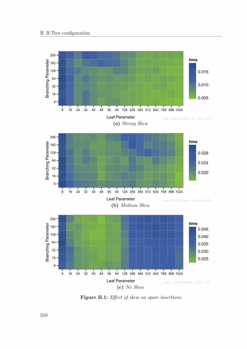
B B-Tree configuration
size: 100000 skew: 0.1 ratio: 100
8
16
32
64
128
192
256
8 16 24 32 40 48 56 64 128 256 384 512 640 768 896 1024
Leaf Parameter
Bra
nchi
ng P
aram
eter
0.005
0.010
0.015
time
(a) Strong Skew
size: 100000 skew: 0.5 ratio: 100
8
16
32
64
128
192
256
8 16 24 32 40 48 56 64 128 256 384 512 640 768 896 1024
Leaf Parameter
Bra
nchi
ng P
aram
eter
0.020
0.024
0.028
time
(b) Medium Skew
size: 100000 skew: 1 ratio: 100
8
16
32
64
128
192
256
8 16 24 32 40 48 56 64 128 256 384 512 640 768 896 1024
Leaf Parameter
Bra
nchi
ng P
aram
eter
0.025
0.030
0.035
0.040
0.045time
(c) No Skew
Figure B.1: Effect of skew on spare insertions
310

size: 100000 skew: all ratio: 10
8
16
32
64
128
192
256
8 16 24 32 40 48 56 64 128 256 384 512 640 768 896 1024
Leaf Parameter
Bra
nchi
ng P
aram
eter
0.006
0.009
0.012
time
(a) Ratio 10
size: 100000 skew: all ratio: 50
8
16
32
64
128
192
256
8 16 24 32 40 48 56 64 128 256 384 512 640 768 896 1024
Leaf Parameter
Bra
nchi
ng P
aram
eter
0.010
0.015
0.020
time
(b) Ratio 50
size: 100000 skew: all ratio: 100
8
16
32
64
128
192
256
8 16 24 32 40 48 56 64 128 256 384 512 640 768 896 1024
Leaf Parameter
Bra
nchi
ng P
aram
eter
0.018
0.021
0.024
0.027
0.030
time
(c) Ratio 100
Figure B.2: Effect of tree-sequence ratio.
311

B B-Tree configuration
size: all skew: all ratio: all
8
16
32
64
128
192
256
8 16 24 32 40 48 56 64 128 256 384 512 640 768 896 1024
Leaf Parameter
Bra
nchi
ng P
aram
eter
0.020
0.025
0.030
0.035
time
(a) All Data
size: all skew: 0.1 ratio: all
8
16
32
64
128
192
256
8 16 24 32 40 48 56 64 128 256 384 512 640 768 896 1024
Leaf Parameter
Bra
nchi
ng P
aram
eter
0.015
0.020
0.025time
(b) Skewed
size: 100000 skew: 1 ratio: 100
8
16
32
64
128
192
256
8 16 24 32 40 48 56 64 128 256 384 512 640 768 896 1024
Leaf Parameter
Bra
nchi
ng P
aram
eter
0.04
0.05
0.06
time
(c) Sparse
Figure B.3: Selection of different heatmaps, showing the B-tree performance fora varying set of parameters (leaf/branching). Each plot depicts a different inputcharacterization. Plot show mixed inputs, comparison to Figure 7.6.
312

size: all skew: all ratio: all
8
16
32
64
128
192
256
8 16 24 32 40 48 56 64 128 256 384 512 640 768 896 1024
Leaf Parameter
Bra
nchi
ng P
aram
eter
0.010
0.015
0.020
0.025
time
(a) All Data
size: all skew: 0.1 ratio: all
8
16
32
64
128
192
256
8 16 24 32 40 48 56 64 128 256 384 512 640 768 896 1024
Leaf Parameter
Bra
nchi
ng P
aram
eter
0.01
0.02
time
(b) Skewed
size: 100000 skew: 1 ratio: 100
8
16
32
64
128
192
256
8 16 24 32 40 48 56 64 128 256 384 512 640 768 896 1024
Leaf Parameter
Bra
nchi
ng P
aram
eter
0.025
0.030
0.035
0.040
0.045time
(c) Sparse
Figure B.4: Selection of different heatmaps, showing the B-tree performance fora varying set of parameters (leaf/branching). Each plot depicts a different inputcharacterization. Plot show removal inputs, comparison to Figure 7.6.
313

B B-Tree configuration
104 105 106 107 108 109 1010 1011 1012 1013
0.005
0.01
0.02
0.05
0.1
0.2Ti
me/
Ele
men
t [μs
]
Sequence Size
● ● ●● ● ● ● ● ● ●
●
●
● ● ● ●
●
●
●
●● ● ● ● ●
●● ●
●●
●●
● ● ● ●● ● ●
●● ●● ● ● ● ● ● ● ●
● mcstl btree 1 2 4 8 16
Figure B.5: Timing measurements for for skewed insertion on M1. Insertionsamong the first 10 percent.
100 200 300 400 500
12
34
56
78
Size
Spe
ed−U
p
● ● ● ● ● ● ● ● ● ● ● ● ● ● ● ● ●
● 2488+8
(a) Correlated (q=0.5)
100 200 300 400 500
12
34
56
78
Size
Spe
ed−U
p
● ● ● ● ● ● ● ● ● ● ●●
●●
● ● ●
● 2488+8
(b) Negatively Correlated (q=-0.5)
Figure B.6: Speed-up of parallel Pareto-optimal shortest path search over thesequential version on M1. The maximal cost of an arc is set to ten.
314

CAppendix C
Continued Measurements onParallel Pareto-search
We present speed-up values for the road instances of Machuca et al.. In addition toFigure 7.11, we provide two additional correlations for comparison in Figure C.2.
12
34
56
NY1NY2
NY3NY4
NY5NY6
NY7NY8
NY9NY10
NY11NY12
NY13NY14
NY15NY16
NY17NY18
NY19NY20
Speed−up
Tim
e [s
]
● ● ● ● ● ● ● ● ● ● ● ● ● ● ● ●●
● ● ●
● 2488+8
Figure C.1: Speed-up of parallel Pareto-optimal shortest path search over thesequential version on M1 on the New-York instances.
315

C Continued Measurements on Parallel Pareto-search
100 200 300 400 500
12
34
56
78
Size
Spe
ed−U
p
● ● ● ● ● ● ● ● ● ● ● ● ● ● ● ● ●
● 2488+8
(a) Negatively Correlated (q=-0.9)
100 200 300 400 5001
23
45
67
8Size
Spe
ed−U
p
● ● ● ● ● ● ● ● ● ● ●●
●●
● ● ●
● 2488+8
(b) Negatively Correlated (q=-0.5)
100 200 300 400 500
12
34
56
78
Size
Spe
ed−U
p
● ● ● ● ● ● ● ● ● ● ● ●● ● ● ●
●
● 2488+8
(c) Uncorrelated (q=0)
100 200 300 400 500
12
34
56
78
Size
Spe
ed−U
p
● ● ● ● ● ● ● ● ● ● ● ● ● ● ● ● ●
● 2488+8
(d) Correlated (q=0.5)
Figure C.2: Speed-up of parallel Pareto-optimal shortest path search over thesequential version on M1. The maximal cost of an arc is set to ten. For highlycorrelated values we barely experience any speed-up. Our standard configurationperforms better in the general case than in the scenario with strongly negativelycorrelated data.
316

DAppendix D
Extended Considerations forthe Penalty Method
To mark dirty cells, we use Algorithm D.1.
Configuration. We tested a range of different setups for the implementation ofCRP-π. Over all of these setups, we visualize the best value for the total distance andevery Dijkstra rank in Figure D.1. Labels along the points mark a change in the besttechnique. A label encodes the type of path penalty (exp = exponential, lin = linearscaling), MA and SA distinguish between singular addition (SA) of rejoin penalty andmultiple application of the rejoin penalty (MA). The following numbers specify thechosen parameters for the penalty, starting with the path penalty. The second numberspecifies the rejoin penalty value. To account for the difference in decision arcs, wetested multiple variations of scaling the respective values for the total distance. Theoverall differences in penalization are minimal, though. Therefore, we were able tochose a uniform penalization scheme.
Timing. For comparison, we also present values on the parallel execution of thepenalization on our machine M1 in Figure D.2.
D.1 Iteration Configuration
Chapter 8 introduced and evolved a way of performing penalized queries on continental-sized networks in a fast and interactive way. We propose a setup that omits the cellsthat contain either the source or the target during the update process. In addition,an efficient implementation should use less than the originally proposed five levelsand especially utilize a smaller than usual cell size for the fourth level. As previouslymentioned, we use a combination of Microcode, the algorithm of Floyd and Warshallfor updating the different cells on the lower levels. For the topmost two levels, we use
317

D Extended Considerations for the Penalty Method
Algorithm D.1 Mark Dirty CellsInput: A graph G (V, A), preprocessed for CRP with associated metric μ, a source
s and a target t, and a path P between s and t.Output: A list of dirty cells
1: Q = ∅2: D = ∅3: for all v ∈ P do4: if cell(v) = cell(s) ∧ cell(v) = cell(t) ∧ !Q.contains(cell(v)) then5: Q.push(cell(v)) � for next iteration6: D.push(cell(v)) � for output7: end if8: end for9: level = 1 � lowest level is zero
10: for level < # levels do11: Q′ = ∅12: for all c ∈ Q do13: if !parent(c).containsAny({s, t}) ∧ !Q′.contains(parent(c)) then14: Q′.push(parent(c)) � for next iteration15: D.push(parent(c)) � for output16: end if17: Q = Q′
18: end for19: end for20: for all c ∈ Q do � topmost level21: D.push(c)22: Q.remove(c)23: end for24: return D
a vectorized implementation of the Bellman-Ford algorithm. The number of levels touse should be determined by the range of the query. Queries of a very short range,up to Dijkstra rank 210, should be restricted to using only a single level. From rank211 through 218, we propose the use of two levels for penalization. For higher Dijkstraranks, the number of levels depends on the allowed usage of parallel computation. Insequential execution, Dijkstra ranks 219 to 221 are fastest using three levels. Abovethis rank four levels perform best. In parallel execution, the settings depend on thenumber of CPUs used. We specify the proposed settings in Table D.1. To decide towhich class of query a certain pair of source and target belongs, a simple lookup tablesuffices that considers the average distance between two pairs of vertices.
We find that omitting the source and target cells for updates results in four levels
318

D.2 Upper Bound Graph
Table D.1: Proposed configuration of the penalization process in dependence ofthe number of used CPUs. The data in this table refers to M2 and specifies themaximum Dijkstra rank for which the number of levels should be used. The depictedranks are to be understood as powers of two.
# CPUs# levels 1 2 4 8 12 16 20 24
one 10 10 9 10 10 10 10 10two 18 16 16 16 16 16 16 16
three 21 19 18 18 18 18 18 18four 24 24 24 24 24 24 24 24
actually outperforming three levels for short- and long-range queries whereas threelevels are best for medium-range queries. The overall cost of the queries is low enoughto justify our ignoring this and keeping to the simple selection method depicted inTable D.1. In addition, the variation we experience for the lower Dijkstra ranks is tobe expected due to the overall very brief time which is required for a single iteration.
Table D.1 shows that the variation we experience for the different number of CPUsstabilizes at four and more CPUs. Only below this threshold a variation seems to benecessary.
D.2 Upper Bound Graph
For illustration, we present a plot of the upper bound graph used in Section 8.2.
319

D Extended Considerations for the Penalty Method
exp−
SA
−1.0
75−0
.007
5
exp−
MA
−1.2
25−0
.005
lin−M
A−1
.225
−0.0
05
exp−
SA
−1.1
1−0.
01
exp−
SA
−1.0
75−0
.007
5
exp−
SA
−1.1
1−0.
01
lin−M
A−1
.225
−0.0
1
01
23
45
67
89
10
210 211 212 213 214 215 216 217 218 219 220 221 222 223 224
Dijkstra rank
Mea
sure
s
linearex
p−S
A−1
.075
−0.0
075
exp−
MA
−1.2
25−0
.005
exp−
MA
−1.0
75−0
.002
5
lin−M
A−1
.225
−0.0
05
exp−
SA
−1.1
1−0.
0075
exp−
SA
−1.0
75−0
.007
5
exp−
SA
−1.1
1−0.
0075
exp−
SA
−1.1
1−0.
01
lin−M
A−1
.225
−0.0
1
01
23
45
67
89
10
210 211 212 213 214 215 216 217 218 219 220 221 222 223 224
Dijkstra rank
Mea
sure
s
sqrt
Figure D.1: Selection method for the final parameters. The points show thedifferent setup methods chosen.
320

D.2 Upper Bound Graph
Dijkstra Rank
Tim
e [m
s] /
Itera
tions
● ● ● ● ● ● ● ● ● ● ● ● ● ● ●
0.01
0.1
110
100
210 211 212 213 214 215 216 217 218 219 220 221 222 223 224
●
InitUpdateQueryAGCTotalIterations
(a) Additional timings on M1 as comparison to Figure 8.15a.
0.1
110
100
●
●
●
●
●
●
●
●
●
●
●
●
●
●●
0.1
110
210 211 212 213 214 215 216 217 218 219 220 221 222 223 224
● 1 Level2 Levels3 Levels4 Levels
Dijkstra Rank
Tim
e [m
s]
Poss
ible
Iter
atio
ns
(b) Eight threads on M1
Figure D.2: Final configuration of CRP-π
321
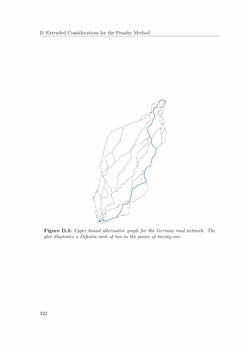
D Extended Considerations for the Penalty Method
Figure D.3: Upper bound alternative graph for the German road network. Theplot illustrates a Dijkstra rank of two to the power of twenty-one.
322

EAppendix E
Additional Information onCorridors
E.1 Random Drives
In addition to the studies already performed in Chapter 11, we present additionalrandom drivers and an extended study of the random walks. The further driversstrengthen the argument that our corridors offer a sub-graph robust to deviations.
The Random Deviation Driver. The most basic driver is the random deviationdriver (RD). He/She operates according to a single parameter p that indicates theprobability for a wrong turn. A random drive by a deviation driver traverses thecorridor, following the given driving directions. At every intersection, we roll a diceand, with probability p, take a wrong turn. The wrong turn itself is chosen uniformlyat random from all incorrect choices available, not considering a potential u-turn.
The Time-Adjusted RD Driver. Our final version that is directly derived from theRD driver. In this version, we follow the notion that a aRD driver’s behavior mightproduce a misleading image in urban areas. In a sequence of short roads, a driver mightfollow the driving directions simply by chance. For our final model, we specify p, p′,and a drop-off function f(t) . As for the aRD, this model increases the probability foran additional wrong turn from p to p′ after the first encountered deviation. Afterwards,depending on the travel time t from the initial mistake, the probability of a wrongturn decreases according to f as long as the driver follows the directions. Every wrongturn resets the probability to p′ and sets the error as new initial mistake. We call thismodel the time-adjusted random deviation driver (taRD).
323

E Additional Information on Corridors
E.1.1 Random WalksIn addition to the previously presented random walks, we present additional plotsshowing the additional drivers. We see only little difference to the drivers alreadycovered in Chapter 11, though. The general observations stay the same.
E.1.2 Corridor GrowthTo give an impression of the growth of an (unfiltered) corridor, we present Figure E.5and Figure E.6. We can see that the turn corridor offers some robustness along allparts of the corridor, whereas the detour corridor may contain long segments withoutdeviation information.
324

E.1 Random Drives
Dijkstra Rank
Suc
cess
Rat
e [%
]
020
4060
8010
0
210 211 212 213 214 215 216 217 218 219 220 221 222 223 224
● ●●
●●
●
● ●
● ●●
●●
●●
● ● ● ●●
● ● ●
● ●
● ● ●
●
●
● ●RD aRD tRD75 tRD85 cRD AR10 AR50 AR100
(a) δt = 100
Dijkstra Rank
Suc
cess
Rat
e [%
]
020
4060
8010
0
210 211 212 213 214 215 216 217 218 219 220 221 222 223 224
●● ●
●● ●
●●
●●
●
●●
●
●
● ● ● ● ● ●● ● ●
● ●● ●
●
●
● ●RD aRD tRD75 tRD85 cRD AR10 AR50 AR100
(b) δt = 200
Figure E.1: Success rate in relation to the length of the shortest path for a detourcorridor; error probability set to ten.
325

E Additional Information on Corridors
Dijkstra Rank
Suc
cess
Rat
e [%
]
020
4060
8010
0
210 211 212 213 214 215 216 217 218 219 220 221 222 223 224
● ●●
●●
●●
●●
●
●
●●
●●
● ●● ● ●
● ●●
●●
●● ●
●
●
● ●RD aRD tRD75 tRD85 cRD AR10 AR50 AR100
(a) δt = 100
Dijkstra Rank
Suc
cess
Rat
e [%
]
020
4060
8010
0
210 211 212 213 214 215 216 217 218 219 220 221 222 223 224
● ● ●● ●
● ●● ●
●
●●
●
●
●
● ● ● ● ● ● ● ● ●●
● ●●
●
●
● ●RD aRD tRD75 tRD85 cRD AR10 AR50 AR100
(b) δt = 200
Figure E.2: Success rate in relation to the length of the shortest path for a recursivedetour corridor (depth of three); error probability set to ten.
326

E.1 Random Drives
Dijkstra Rank
Suc
cess
Rat
e [%
]
020
4060
8010
0
210 211 212 213 214 215 216 217 218 219 220 221 222 223 224
●
●
●
●●
●
●
●●
●●
●● ● ●
● ●● ●
● ●●
●●
●●
● ●
●
●
● ●RD aRD tRD75 tRD85 cRD AR10 AR50 AR100
(a) One turn
Dijkstra Rank
Suc
cess
Rat
e [%
]
020
4060
8010
0
210 211 212 213 214 215 216 217 218 219 220 221 222 223 224
● ● ● ● ● ● ● ● ●●
● ●●
●
●
● ● ● ● ● ● ● ● ● ● ● ● ● ● ●
● ●RD aRD tRD75 tRD85 cRD AR10 AR50 AR100
(b) Three turns
Figure E.3: Success rate in relation to the length of the shortest path for a turncorridor; error probability set to ten.
327

E Additional Information on Corridors
Dijkstra Rank
Suc
cess
Rat
e [%
]
020
4060
8010
0
210 211 212 213 214 215 216 217 218 219 220 221 222 223 224
●●
● ●● ●
● ● ●●
● ●●
●
●
● ● ● ● ● ● ● ● ● ● ● ●● ●
●
● ●RD aRD tRD75 tRD85 cRD AR10 AR50 AR100
(a) Detour corridor; δt = 500
Dijkstra Rank
Suc
cess
Rat
e [%
]
020
4060
8010
0
210 211 212 213 214 215 216 217 218 219 220 221 222 223 224
● ● ● ● ● ● ● ● ● ● ● ● ● ● ●● ● ● ● ● ● ● ● ● ● ● ● ● ● ●
● ●RD aRD tRD75 tRD85 cRD AR10 AR50 AR100
(b) Turn corridor; six turns
Figure E.4: Success rate in relation to the length of the shortest path for a detourcorridor; error probability set to ten.
328

E.1 Random Drives
(a) One turn
(b) Two turns
(c) Three turns
(d) Four turns
(e) Five turns
Figure E.5: Turn corridor for a varying number of turns (rank 219).
329

E Additional Information on Corridors
(a) δt = 10
(b) δt = 50
(c) δt = 100
(d) δt = 200
(e) δt = 500
Figure E.6: Detour corridor for a varying size of δt (rank 219).
330

FAppendix F
Further Comparisons
For additional comparison, we present figures depicting the quality of the first alternativeroute as well as the success rates for the first three alternatives here. The alternativeroutes have been extracted using the linear combination selection strategy. We can seethat penalty methods (Figure F.3) offer a the best success rate in general. The largestdifference in the success rate can be found for short-range to mid-range queries. For thesetypes of queries, even the corridors methods can be considered viable (c.f. Figure F.1).The quality, in terms of Definition 5.3 (bounded stretch (BS), local optimality (LO),limited sharing (α) ) is better for the via-vertex method (c.f. Figure F.2), though.
331

F Further Comparisons
●●
●●
● ● ● ● ●●
●●
● ● ● ● ● ● ● ● ●
●
● ● ● ●●
●
●
●
●
●
●
●●
● ● ● ●●
●●
●●
●
●
010
3050
7090
01
23
45
67
89
10
21 22 23 24 25 26 27 28 29 210 211 212 213 214 215 216 217 218 219 220 221 222 223 224
Dijkstra Rank
Para
met
er V
alue
● ●1st2nd3rd
αβε
(a) Success rates and quality values for first alternative for a three-recursive detourcorridor. Initial detour: twenty seconds.
●
●
● ●
●● ●
● ● ● ●● ●
● ● ● ● ● ● ● ●●
●
● ● ●●
●
●
●●
●●
●● ●
● ● ● ● ●●
●●
●
●
●
010
3050
7090
01
23
45
67
89
10
21 22 23 24 25 26 27 28 29 210 211 212 213 214 215 216 217 218 219 220 221 222 223 224
Dijkstra Rank
Para
met
er V
alue
● ●1st2nd3rd
αβε
(b) Success rates and quality values for first alternative for a six-turn corridor.
Figure F.1: Quality of our corridor approaches
332

●
●
●
●● ●
●● ● ●
● ●● ● ● ● ● ● ●
● ●
●
● ● ● ●●
●
●●
●●
●
●●
● ●●
●● ●
●●
●●
●
010
3050
7090
01
23
45
67
89
1021 22 23 24 25 26 27 28 29 210 211 212 213 214 215 216 217 218 219 220 221 222 223 224
Dijkstra Rank
Para
met
er V
alue
● ●1st2nd3rd
αβε
Figure F.2: Success rates and quality values for first alternative for HiDAR.
333

F Further Comparisons
●
● ●
●●
● ●● ● ● ● ● ● ● ● ●
● ●● ● ●
●
●
● ●●
●
●
●
●
●
●●
●
●● ● ●
●● ●
●
●●
●● ●
010
3050
7090
01
23
45
67
89
10
21 22 23 24 25 26 27 28 29 210 211 212 213 214 215 216 217 218 219 220 221 222 223 224
Dijkstra Rank
Para
met
er V
alue
● ●1st2nd3rd
αβε
(a) Success rates and quality values for first alternative for CRP-π.
●
●
●●
● ●● ● ● ●
● ● ● ● ● ● ●● ●
● ●
●
● ● ●●
●
●●
●
●
●
●
●
● ● ●
● ● ●
●
●●
●● ●
010
3050
7090
01
23
45
67
89
10
21 22 23 24 25 26 27 28 29 210 211 212 213 214 215 216 217 218 219 220 221 222 223 224
Dijkstra Rank
Para
met
er V
alue
● ●1st2nd3rd
αβε
(b) Success rates and quality values for first alternative for CRP-∞.
Figure F.3: Quality of our penalization approaches
334