Asymptotic Reasoning - Computational Logic
140
Lehrstuhl für Logik und Verifikation Fakultät für Informatik Technische Universität München Manuel Eberl Asymptotic Reasoning in a Proof Assistant
-
Upload
khangminh22 -
Category
Documents
-
view
0 -
download
0
Transcript of Asymptotic Reasoning - Computational Logic
Lehrstuhl für Logik und VerifikationFakultät für InformatikTechnische Universität München
Manuel Eberl
Asymptotic Reasoningin a Proof Assistant

Lehrstuhl für Logik und VerifikationFakultät für InformatikTechnische Universität München
Asymptotic Reasoning in a Proof Assistant
Manuel Eberl
Vollständiger Abdruck der von der Fakultät für Informatik der Technischen Universität Münchenzur Erlangung des akademischen Grades eines
Doktors der Naturwissenschaften (Dr. rer. nat.)
genehmigten Dissertation.
Vorsitzender:Prof. Dr. Helmut Seidl
Prüfende der Dissertation:1. Prof. Tobias Nipkow, Ph.D.2. Prof. Dr. Sander R. Dahmen,Vrije Universiteit Amsterdam
Die Dissertation wurde am 21.09.2020 bei der Technischen Universität München eingereicht unddurch die Fakultät für Informatik am 01.12.2020 angenommen.


Abstract
This dissertation describes my work in the formalisation of mathematics with the proofassistant Isabelle/HOL, particularly mathematics related to asymptotic concepts such as limitsand function growth. This work consists of both the formalisation of fundamental mathemat-ical material for the Isabelle/HOL standard library and the creation of new proof automationtools. Both of these have since been used successfully in many formalisation applicationsboth in pure mathematics (such as analysis and number theory) and computer science (i.e.algorithm analysis).
Specically, this thesis presents four major contributions, each corresponding to one peer-reviewed publication under the umbrella of ‘asymptotic reasoning in Isabelle/HOL’:
The rst of these introduces a proof automation tool that employs techniques from computeralgebra to compute and prove limits and other asymptotic properties for a large class ofreal-valued functions (much like systems such as Maple or Mathematica). This tool has beeninstrumental in all my subsequent formalisation work, and no comparable instrumentationexists in other proof assistants.Second, a formal proof of a ‘cookbook method’ theorem due to Akra and Bazzi, which is
a sweeping generalisation of the well-known Master Theorem of divide-and-conquer recur-rences. In computer science, this theorem is a staple of the analysis of divide-and-conqueralgorithms. The formalisation also provides tooling to facilitate the application of the theoremto specic algorithms.
Third, a formalisation of the theory of linear recurrences and rational generating functions– in particular how to obtain closed-form solutions and asymptotic estimates of linear recur-rences. These have applications in combinatorics and in the analysis of algorithms and datastructures. In addition to the theorems, a veried executable solver for linear recurrences anda certier for their asymptotics are also provided.
Finally, in order to demonstrate the usability of the aforementioned library and machinery,the last publication then describes its application to the formalisation of the vast majority ofApostol’s classic textbook on analytic number theory, including the Prime Number Theorem,Dirichlet’s Theorem, and many more results on the distribution of prime numbers and theasymptotic behaviour of number-theoretic functions.
iii

Zusammenfassung
Diese Dissertation beschreibt meine Arbeit in der Formalisierung von Mathematik mit demBeweisassistenten Isabelle/HOL, insbesondere von Mathematik im Zusammenhang mit asym-ptotischen Konzepten wie Grenzwerten und Funktionswachstum. Diese Arbeit beinhaltetsowohl die Formalisierung grundlegenden mathematischen Materials für die Isabelle/HOL-Standardbibliothek als auch die Etablierung neuer Werkzeuge zur Beweisautomatisierung.Beides wurde seitdem erfolgreich in vielen Anwendungen eingesetzt, sowohl Formalisierun-gen in der reinen Mathematik (wie Analysis und Zahlentheorie) als auch in der Informatik (z.B. Algorithmenanalyse).Konkret besteht diese Arbeit aus vier Teilen im Bereich „asymptotische Beweisführung in
Isabelle/HOL“ mit jeweils einer zugehörigen Veröentlichung:Der erste Teil ist ein Werkzeug zur Beweisautomatisierung, das Techniken aus der Com-
puteralgebra verwendet, um Grenzwerte und andere asymptotische Eigenschaften für einegroße Klasse von reellen Funktionen zu berechen und zu beweisen (ähnlich wie Systeme wieMaple oder Mathematica).Der zweite Teil beschreibt den formalen Beweis eines kochrezeptartigen Theorems von
Akra und Bazzi, das eine Verallgemeinerung des bekannten Master-Theorems für „divide-and-conquer“-Rekurrenzen darstellt. Dieses Theorem ist ein grundlegender Bestandteil derAnalyse von „divide-and-conquer“-Algorithmen in der Informatik. Die Formalisierung bein-haltet außerdem Werkzeuge, die die Anwendung des Theorems auf konkrete Algorithmenangenehmer gestalten.Der dritte Teil ist die Formalisierung der Theorie der linearen Rekurrenzen und rationa-
len Erzeugendenfunktionen – insbesondere wie geschlossene Lösungen und asymptotischeAbschätzungen für sie gewonnen werden können. Diese nden Anwendungen in der Kom-binatorik und der Analyse von Algorithmen und Datenstrukturen. Zusätzlich werden einverizierter ausführbarer Löser sowie eine Zertizierer für asymptotische Abschätzungenentwickelt.Als letzter Punkt wird, um die Nutzbarkeit der zuvor dargelegten Bibliothek und Maschi-
nerie zu zeigen, die Formalisierung des Großteils von Apostols Lehrbuch über analytischeZahlentheorie geschildert. Dies beinhaltet formale Beweise für den Primzahlsatz, den Satz vonDirichlet, und viele andere Resultate über die Verteilung der Primzahlen und das asymptoti-sche Verhalten zahlentheoretischer Funktionen.
iv

Acknowledgements
This section was by far the easiest one for me to write, since there is simply so much towrite about. The dicult part was really where to stop.
First of all, I would like to thank everyone who commented on or helped with any of thepublications upon which this thesis is based: Jeremy Avigad, Louay Bazzi, Max Haslbeck (theelder), Johannes Hölzl, Kristina Magnussen, Tobias Nipkow, Andrei Popescu, and the numer-ous anonymous reviewers. I also want to additionally thank the people who commented onthe thesis text itself: Mathias Fleury, Jasmin Blanchette, Max Haslbeck (the elder), Lars Hupel,Mohammad Abdulaziz, Jeremy Avigad, Uma Zalakain, Simon Wimmer, Kevin Buzzard, JulianBrunner, and Kristina Magnussen.
Next, I have to talk about the group I worked at in Munich. I had the great fortune to work inTobias Nipkow’s group as a PhD student for six years, and to be vaguely unocially associatedwith it for a few years before that. I will thank a great number of people I met during thattime. I tried to keep it short, failed, and decided it did not matter.
First, Peter ‘The Machine’ Lammich, who was the advisor of my rst Bachelor’s thesis and‘Praktikum’. He was probably the most athletic member of our group (which is no small feat,given the competition), and he is basically a one-man research group all by himself. His moveto Brexitland was a great loss for us all.
Johannes Hölzl, the advisor of my Master’s thesis, and Fabian Immler, my next-door oceneighbour. They were the two mathematicians of the chair’s old guard, and their departureleft me as their rather inadequate replacement as resident expert for probability theory andanalysis.
Julian Brunner, who introduced me to the world of competitive Super Smash Bros. Melee forthe Nintendo GamecubeTM and who served as my partner-in-crime for our highly successfulelectronics project (the rst USB Sledgehammer) and our not-so-successful lm project.Ondřej Kunčar, who loved nothing more than to give me (and everyone else) an excuse
not to work by starting lengthy discussions. I miss arguing about minutiæ of word usage inGerman with eight other native speakers during lunch due to one of his questions.
Mohammad Abdulaziz, always in the mood for a lengthy Socratic dialogue where he wouldcontinually ask me things about a topic I thought I knew something about until I felt like Iabsolutely did not. He was always easily convinced to join into whatever activity I proposed,be it bouldering, Super Smash Bros., or climbing Arthur’s Seat.
Lars Noschinski, who was in the last year of his PhD when I was in my rst. His sueringserved as a chilling omen of what it would be like to write up a thesis.
v

Jonas Rädle, Kevin Kappelmann, and Lukas Stevens, the Nesthäkchen who managed to puttogether a very respectable Haskell lecture between the three of them and graciously allowedme to serve as Master of Competition (Sr).
Jasmin Blanchette, an amazing polyglot (certainly much more so than I!) and never-endingfountain of productivity (likewise). He was also the originalMaster of Competition and, havinginherited the position from him, I can only hope I did my job half as well as he did.
Dmitriy Traytel – a pub quiz enthusiast (like me) and a PhD speedrunner (unlike me). Hiswork on corecursion solved some of my problems years before I knew I had them. I will notpretend I understand any of it, but fortunately it was easy enough to use.
Max Haslbeck (the elder), my climbing instructor, who continuously pushes me to try harderproblems. Even outside the gym, he is always full of suggestions and enthusiasm.Simon Wimmer, aspiring ecoterrorist and fellow Gymnasium Dingolng alumnus. Of all
the members of our bouldering group, he was the one closest to me in skill, so it was alwaysgreat fun to send with him.
Helma Piller (and before her Eleni Nikolaou-Weiss), who somehow keeps this unruly lot ofus suciently organised. Without her, we would probably all have long since been bankruptedby unreimbursed travel expenses.Finally, m’colleague, Lars Hupel. Fellow connoisseur of good dogs and bad puns. I very
much miss his absurd enthusiasm for trains, electoral systems, and bureaucracy, and his mor-bid interest in looking at a piece of software and nding the most bizarre and disgusting thinghe can get it to do. I also really miss him getting the water for our Earl Grey. I mean, that teakitchen is denitely too far away.
To prevent this section from exploding even more, I will only briey mention a numberof other people who helped or inuenced me in some way, and/or from whose prior work Ihave proted greatly: Florian Brandl, Felix Brandt, Amine Chaieb, Jacques Fleuriot, ChristianGeist, Florian Haftmann, John Harrison, Joris van der Hoeven, Brian Human, Gregor Kemper,Angeliki Koutsoukou-Argyraki, Alexander Krauss, Wenda Li, Larry Paulson, Andrei Popescu,Bruno Salvy, René Thiemann, Thomas Türk, Akihisa Yamada, Bohua Zhan. I would also espe-cially like to thank Larry Paulson for hosting me in Cambridge for ve very productive weeks,and the CeDoSIA graduate school for paying for it.
Of course, I also want to profusely thank my advisor Tobias Nipkow. He introduced me tothe world of Interactive Theorem Proving back in 2011 and supported me all the way untilnow in 2020, always giving me great freedom to pursue my own interests, perhaps with theoccasional little nudge in the right direction. He has cultivated an exceptional group of peoplein Munich and I could not have found a better place to work in.
Lastly, I would also like to thank my girlfriend of many years, Kristina Magnussen, and myparents and my grandmother for their support during all those years.
vi

Contents
1 Introduction 1
2 Outline 7
3 Preliminaries 93.1 The Isabelle Proof Assistant . . . . . . . . . . . . . . . . . . . . . . . . . . . . 93.2 Interactive Theorem Proving in a Nutshell . . . . . . . . . . . . . . . . . . . . 103.3 The Isabelle Distribution and the Archive of Formal Proofs . . . . . . . . . . . 143.4 Notation and Terminology . . . . . . . . . . . . . . . . . . . . . . . . . . . . . 153.5 Landau Symbols . . . . . . . . . . . . . . . . . . . . . . . . . . . . . . . . . . . 17
4 Summary of Contributions 21
5 Semi-Automatic Real Asymptotics 235.1 Multiseries . . . . . . . . . . . . . . . . . . . . . . . . . . . . . . . . . . . . . . 255.2 Implementation . . . . . . . . . . . . . . . . . . . . . . . . . . . . . . . . . . . 285.3 Asymptotic Interval Arithmetic . . . . . . . . . . . . . . . . . . . . . . . . . . 295.4 Related Literature . . . . . . . . . . . . . . . . . . . . . . . . . . . . . . . . . . 305.5 Future Work and Outlook . . . . . . . . . . . . . . . . . . . . . . . . . . . . . . 30
6 Divide-and-Conquer Recurrences 336.1 The Formalised Theorem . . . . . . . . . . . . . . . . . . . . . . . . . . . . . . 336.2 Automation . . . . . . . . . . . . . . . . . . . . . . . . . . . . . . . . . . . . . 356.3 Related Literature . . . . . . . . . . . . . . . . . . . . . . . . . . . . . . . . . . 36
7 Linear Recurrences 397.1 Denitions and Scope . . . . . . . . . . . . . . . . . . . . . . . . . . . . . . . . 407.2 Implementation . . . . . . . . . . . . . . . . . . . . . . . . . . . . . . . . . . . 417.3 Certifying Asymptotic Upper Bounds . . . . . . . . . . . . . . . . . . . . . . . 417.4 Related Literature and Applications . . . . . . . . . . . . . . . . . . . . . . . . 42
8 Analytic Number Theory 438.1 Formalised Results . . . . . . . . . . . . . . . . . . . . . . . . . . . . . . . . . . 438.2 Related Literature . . . . . . . . . . . . . . . . . . . . . . . . . . . . . . . . . . 448.3 Further Work . . . . . . . . . . . . . . . . . . . . . . . . . . . . . . . . . . . . 45
9 Concluding Remarks 47
Bibliography 51
vii
Contents
Appendix 59
A Semi-Automatic Real Asymptotics 61
B Divide-and-Conquer Recurrences 71
C Analytic Number Theory 99
D Linear Recurrences 119
viii

1 Introduction
“ [The Analytical Engine] might act upon other things besides number, were objectsfound whose mutual fundamental relations could be expressed by those of theabstract science of operations, and which should be also susceptible of adaptationsto the action of the operating notation and mechanism of the engine.— Ada Lovelace, Sketch of the Analytical Engine (1842) ”“ Wir sehen seit langem, daß diese Maschinen sich zu mehr eignen als zur planvol-
len Verarbeitung von Zahlen, vielmehr zu jeder in Regeln faßbaren Behandlungvon Informationen irgendwelcher Art.
We have long been able to see that these machines lend themselves to more than thesystematic processing of numbers, but rather to handling information of any kindin any way that can be expressed in rules.
— Eike Jessen, Die elektronische Rechenmaschine und unsere Gesellschaft (1969) ”At the beginning of the 20th century, there was a erce debate among mathematicians: canmathematics be made fully formal, i.e. expressed using only symbols and a few reasoningrules? Or are there some parts of it that transcend formalism? Some, such as Hilbert, stronglybelieved that formalisingmathematics was not only possible, but necessary. All of mathematicsshould be put on formally rigorous and provably consistent foundations. It was even imaginedthat one day one might be able to construct a machine that could eventually decide the validityof any mathematical statement at the push of a button.
Unfortunately, these hopes were squashed by Gödel’s groundbreaking incompleteness the-orems in 1931, which, arguably, imply that there can be no such unied formal frameworkfor mathematics. Informally, the statements of these two theorems are that any sucientlypowerful and consistent mathematical framework will have two aws:
• There are true statements for which no proof exists.• The consistency of the framework cannot be proven within itself.
Some years later, Turing showed a related result: the undecidability of the halting problem, i.e.that there cannot be a computer program which, given another computer program 𝑃 as input,decides whether 𝑃 terminates or not. This also implies that the ‘magic button machine’ cannotexist: if it did, we could simply encode ‘𝑃 terminates’ as a mathematical statement, push thebutton, and return that result.11Turing’s result in fact implies a variant of Gödel’s rst theorem: if all true statements could be proven, then foreach program 𝑃 there would be a proof for ‘𝑃 terminates’ or ‘𝑃 does not terminate’, and we could solve thehalting problem by searching the space of all proofs until we nd a proof for either of the two statements.
1

1 Introduction
However, this was not the end of formal mathematics: one could still hope to nd a formalframework that works well in practice, i.e. we just hope that whatever statement we currentlycare about will turn out to be provable. In 1901, Russell’s paradox (‘the set of all sets thatdo not contain themselves’) seemed to cast doubt on this, since it showed that the naïve settheory that was used at the time was fundamentally awed as a logical system. Some believedthat this only showed that formal mathematics was a fool’s errand to begin with, but variouslogicians worked on solutions to this in the following years that have since turned out to bequite robust. Russell himself developed a new system based on the notion of types with theintention of preventing the kind of self-referentiality that led to the paradox he had discovered.
Based on this, Whitehead and Russell set it upon themselves to create the rst fully formaland rigorous collection of mathematics: the Principia Mathematica. It is an enormous three-volume work, over ten years in the making and with over two thousand pages combined. In it,they attempted to develop mathematics absolutely formally from the ground up with a level ofrigour that had never been seen before, at a time when symbolic logic was still in its infancy.They began with set theory, basic arithmetic, and real numbers, but having reached the end ofthe third volume in 1913, they admitted to being ‘intellectually exhausted’ and gave up on theirplans on a fourth volume on geometry. The Principia’s lengthy proof leading up to the factthat 1 + 1 = 2 is frequently used to poke fun at formal mathematics, and the book is certainlyalmost impossible to read. Fittingly, the historian Peter Watson called it ‘one of Russell’s mostoriginal publications’ but also ‘one of the least read of modern times.’ Nevertheless, they hadachieved one important goal: by the time they had written it, it was widely accepted that therewere probably no fundamental obstacles to formalising all of known mathematics.
Although it had now been shown that formalising mathematics was possible in principle,it seemed completely infeasible to do so for any signicant amount of non-trivial material.However, only a few years later, a real game changer appeared on the scene: the electroniccomputer. With it came the possibility of outsourcing the tedious and error-prone task ofwriting and checking formal proofs to a machine. And indeed, in 1956, Newell et al. wrotethe computer program Logic Theorist, the rst automated theorem prover. It was able to ndproofs for 38 of the rst 52 theorems from the Principia, and in one instance the proof it foundwas more elegant and satisfying than the one in the Principia. In a letter to Simon (one of theauthors of Logic Theorist), Russell commented:
‘I am delighted to know that Principia Mathematica can now be done by machinery[. . . ] I am quite willing to believe that everything in deductive logic can be doneby machinery.’
McCorduck expressed this in more philosophically coloured words in her book ‘MachinesWho Think’ [77], stating that the success of Logic Theorist was ‘proof positive [that] a ma-chine could perform tasks heretofore considered intelligent, creative, and uniquely human’.
While these automated theorem provers (ATP) are without doubt a thriving and importantarea of research, they are not the topic of my work, and they do have their limitations: we arestill very far away from giving a dicult (or even open) problem in mathematics to a computerand having any hope of it nding a proof in our lifetime. There has been one notable case
2
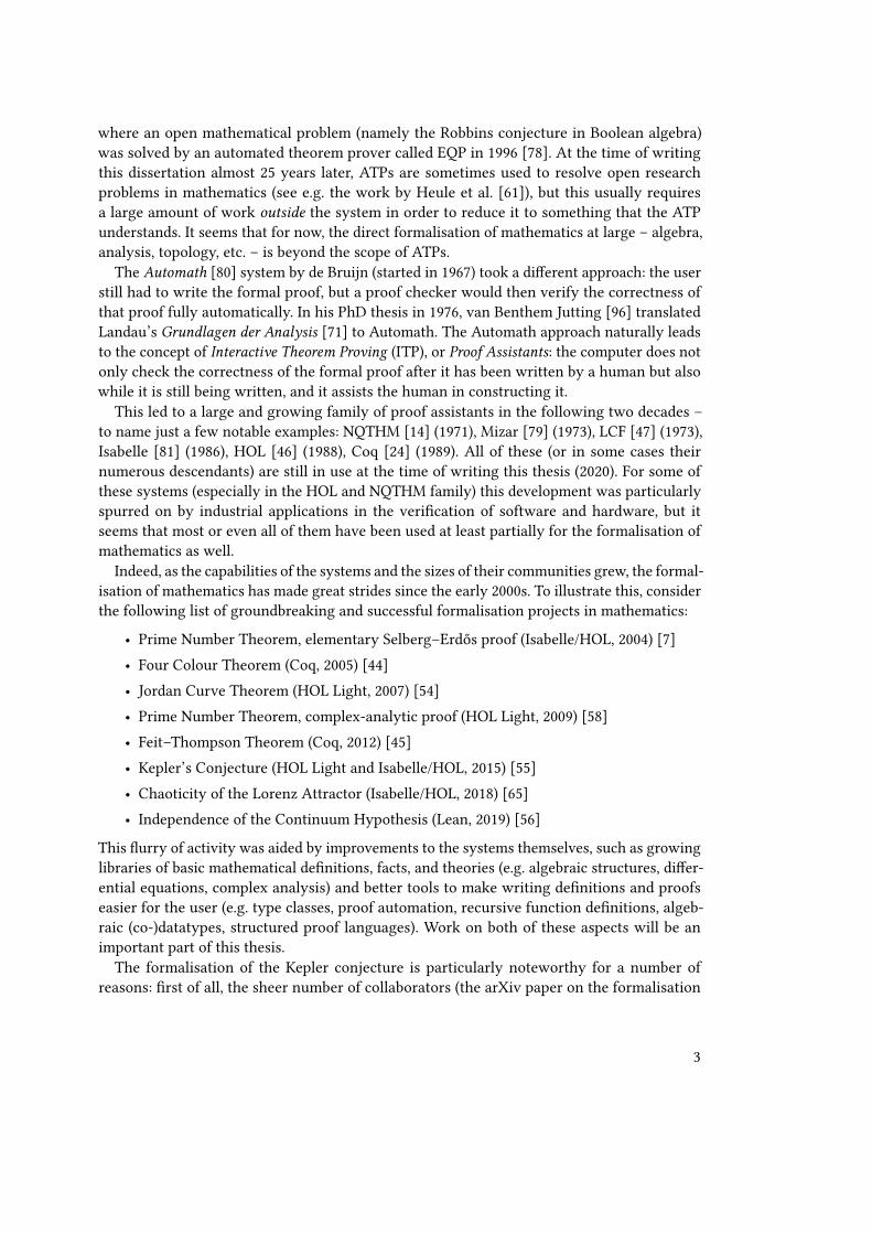
where an open mathematical problem (namely the Robbins conjecture in Boolean algebra)was solved by an automated theorem prover called EQP in 1996 [78]. At the time of writingthis dissertation almost 25 years later, ATPs are sometimes used to resolve open researchproblems in mathematics (see e.g. the work by Heule et al. [61]), but this usually requiresa large amount of work outside the system in order to reduce it to something that the ATPunderstands. It seems that for now, the direct formalisation of mathematics at large – algebra,analysis, topology, etc. – is beyond the scope of ATPs.
The Automath [80] system by de Bruijn (started in 1967) took a dierent approach: the userstill had to write the formal proof, but a proof checker would then verify the correctness ofthat proof fully automatically. In his PhD thesis in 1976, van Benthem Jutting [96] translatedLandau’s Grundlagen der Analysis [71] to Automath. The Automath approach naturally leadsto the concept of Interactive Theorem Proving (ITP), or Proof Assistants: the computer does notonly check the correctness of the formal proof after it has been written by a human but alsowhile it is still being written, and it assists the human in constructing it.
This led to a large and growing family of proof assistants in the following two decades –to name just a few notable examples: NQTHM [14] (1971), Mizar [79] (1973), LCF [47] (1973),Isabelle [81] (1986), HOL [46] (1988), Coq [24] (1989). All of these (or in some cases theirnumerous descendants) are still in use at the time of writing this thesis (2020). For some ofthese systems (especially in the HOL and NQTHM family) this development was particularlyspurred on by industrial applications in the verication of software and hardware, but itseems that most or even all of them have been used at least partially for the formalisation ofmathematics as well.
Indeed, as the capabilities of the systems and the sizes of their communities grew, the formal-isation of mathematics has made great strides since the early 2000s. To illustrate this, considerthe following list of groundbreaking and successful formalisation projects in mathematics:
• Prime Number Theorem, elementary Selberg–Erdős proof (Isabelle/HOL, 2004) [7]• Four Colour Theorem (Coq, 2005) [44]• Jordan Curve Theorem (HOL Light, 2007) [54]• Prime Number Theorem, complex-analytic proof (HOL Light, 2009) [58]• Feit–Thompson Theorem (Coq, 2012) [45]• Kepler’s Conjecture (HOL Light and Isabelle/HOL, 2015) [55]• Chaoticity of the Lorenz Attractor (Isabelle/HOL, 2018) [65]• Independence of the Continuum Hypothesis (Lean, 2019) [56]
This urry of activity was aided by improvements to the systems themselves, such as growinglibraries of basic mathematical denitions, facts, and theories (e.g. algebraic structures, dier-ential equations, complex analysis) and better tools to make writing denitions and proofseasier for the user (e.g. type classes, proof automation, recursive function denitions, algeb-raic (co-)datatypes, structured proof languages). Work on both of these aspects will be animportant part of this thesis.The formalisation of the Kepler conjecture is particularly noteworthy for a number of
reasons: rst of all, the sheer number of collaborators (the arXiv paper on the formalisation
3
1 Introduction
lists 22 authors); second, the conjecture had only been resolved a few years before formalisationbegan. The proof by Hales relied heavily on computations done by computer programs writtenspecically for the proof and the referees found themselves overwhelmed by the task ofchecking the correctness of these programs. This led Hales – a mathematician with no priorassociation with the theorem-proving community – to spearhead the formalisation eorthimself. This illustrates a rst and very important reason why formalisation of mathematicsmight be interesting both to mathematicians and to society in general: it allows us to convinceourselves beyond reasonable doubt that a mathematical proof is correct when the traditionalrefereeing process fails, such as for computer proofs.The other projects mentioned above were also very daunting at the time. For instance,
shortly before Harrison formalised the analytic proof of the Prime Number Theorem in HOLLight, Bob Solovay had predicted2 that proof assistants would not be ready to formalise thisproof for decades. This brings us to another reason to formalise mathematics: to demonstratethat it can be done.
The last reason is an even more frivolous one but a very important one to me nonetheless:Because it is fun. There is a profound satisfaction innate to formalisation with a proof assistantthat can only be compared to mastering an exceptionally dicult computer game (a compar-ison e.g. made half-jokingly by Tobias Nipkow when introducing the Isabelle proof assistantin his Semantics lecture). The formaliser (or player) tackles one proof obligation after another,frantically working back and forth to make a connection between the assumptions and thegoal, backtracking and trying another route when entering a dead end, and rejoicing uponnally reaching ‘No subgoals!’. While this may sound just like ‘pen-and-paper’ mathematics,the dierence is that the computer, ever vigilant and pedantic, gives immediate feedback atevery single step and does not allow even the slightest vagueness in an argument. There ishardly ever any uncertainty about whether what one has written down is correct or not. Thus,the feedback loop of punishment and reward is very fast – just like in a computer game.
I discovered this computer game in my rst year as an undergraduate in 2011 in the afore-mentioned lecture by Tobias Nipkow. The ability to formalise arbitrary statements from com-puter science and mathematics at this level of clarity immediately impressed and fascinatedme greatly.3 It is no exaggeration to say that this experience completely derailed the course ofmy university studies – but unlike other highly addictive computer games, it was probably notto the detriment of my academic career. From that point onward, it was interactive theoremproving all the way for me, and that has now led me to this PhD project.
2See the paragraph on the Prime Number Theorem in FreekWiedijk’s ‘The Seventeen Provers of theWorld’ [101].3Indeed, in my experience, many mathematicians still seem to be under the impression that this is not possible. Aparticularly common misconception is that because they have nite memory, computers can only ever checknitely many cases by exhaustion but not possibly reason about innity and non-discrete objects like realnumbers or transcendental functions. An odd thing to think, in my opinion, considering they seem to be ableto do it just ne with a nite brain and a nite piece of paper in front of them. Perhaps this is a remnant of theaforementioned idea that mathematical reasoning is something ‘intelligent, creative, and uniquely human.’
4

In this publication-based thesis, I will showcase four particular steps from one importantpart of my interactive theorem proving journey. These correspond to four peer-reviewedarticles of mine that can be found in the appendix, bound together by the common theme ofasymptotics: the study of limits and the growth of (mostly real-valued) functions, a topic thathad previously not been given enough attention in our community.
5

2 Outline
As stated before, the thesis is centred around four peer-reviewed publications, which canbe found in the appendix. Most of the remainder of the thesis serves to provide summaries,background information, and context for these.Chapter 3 gives some general background required to understand the work that is being
presented: Section 3.1 presents a brief overview of the Isabelle theorem prover, followed by amore detailed explanation of how interactive theorem proving is done in Isabelle in practice inSection 3.2. Section 3.3 explains the visible universe of Isabelle applications, where formalisedmaterial in Isabelle is published, and how it is maintained. Lastly, Section 3.4 explains somenotational conventions and terminology relevant to the rest of this work and Section 3.5focuses in particular on the asymptotic notation known as Landau symbols.Next, Chapter 4 gives a brief synopsis of the four publications as well as a short list of
additional related contributions without a formal publication attached to them. Chapters 5 to 8then each give more detailed summaries, motivation, background information, and in somecases outlook regarding one of the publications.Finally, Chapter 9 concludes with some additional noteworthy formalisation work that I
have done during my time as a PhD student and some remarks on what I consider importantfor the future of the formalisation of mathematics.
7


3 Preliminaries
“ Formal verication is like opening cans of worms,and then eating them.
— Robert Sison, via Twitter (2020) ”3.1 The Isabelle Proof Assistant
For the work presented in this thesis (and all of my work in general), I used the proof assistantIsabelle, which was originally developed by Larry Paulson in 1986 and extended by variousother people after that, including me. What sets Isabelle apart frommost other proof assistantsis the fact that it is generic: it provides a very minimalistic logic called Isabelle/Pure, whichonly provides very basic logical concepts such as implication and universal quantication. Ontop of this, various other object logics can be (and have been) built. At the time of writing thisdissertation, the most used logic in Isabelle by a very large margin is higher-order logic (HOL),and this is the logic that I used as well. Isabelle’s version of HOL is very similar to those of theother systems from the HOL family of proof assistants (e.g. HOL4, HOL Light, HOL Zero, ProofPower), and there is ongoing work on importing HOL4 proofs into Isabelle/HOL [66]. For thesake of completeness, I will mention two other object logics available in Isabelle. First, thereis Zermelo–Fraenkel set theory, which is considered the usual ‘default’ logic for traditionalmathematics (but is not very well-developed in Isabelle). Second, there is recent and veryambitious work to create support for Homotopy Type Theory as well [22].
Any theorem proving system that is usable for practical developments will likely consist ofa fairly large code base. Consequently, steps must be taken to still ensure the soundness of theoverall system, i.e. that any theorem that can be produced by the system really is a valid factin the underlying logic. There are various approaches for this, but I will only mention the oneused by Isabelle: like the systems of the HOL family, the design of Isabelle roughly followswhat is known as the LCF model (named after the early experimental theorem prover of thesame name). The full formal proofs (also called proof terms or proof objects) are not recordedat all. Soundness is instead ensured through a mechanism of the programming language inwhich the system is implemented (Standard ML). A type thm of theorems is dened in such away that only a relatively small set of functions can inspect and manipulate values of this type.These functions form the inference kernel, and all other code can only create or modify suchthm values by using this kernel. Therefore, in principle, only the correctness of the kernelis critical for the soundness of the resulting system. The kernel is relatively small and onlyprovides very basic operations such as modus ponens, eliminating a universal quantier, ormaking a non-recursive equational denition.
9

3 Preliminaries
The Standard ML implementation and runtime that Isabelle is based upon is Poly/ML [76],which allows on-the-y compilation of code. Isabelle makes use of this by providing an MLcommand with which users can add arbitrary program code to the system at any point (manyother systems have similar features). This allows advanced users to create their own Isabellecommands, including proof automation, denitional tools, diagnostic and visualisation tools,or interfaces to external tools (such as automated theorem provers or computer algebra sys-tems). Regarding user-dened proof automation tools, it should again be mentioned that dueto the LCF approach, bugs in user code cannot lead to logical inconsistencies by design. Inter-estingly, most of Isabelle’s basic commands are not ‘built-in’ but also constructed in this waywith only a fairly minimal amount of bootstrapping. In this sense, there is no clear distinctionbetween an Isabelle user and an Isabelle developer.
Lastly, I must mention one very important feature of Isabelle, even if it is only tangentiallyrelevant for the work presented here: the code generator [52, 53]. Isabelle’s code generator canautomatically generate executable code from Isabelle/HOL denitions, provided that thesedenitions fall within a suitable ‘computational’ subset of HOL (e.g. no unbounded quantic-ation or choice operators). For denitions that are not directly computational in this sense orthat are too inecient, code equations can be provided. These are ‘alternative denitions’ tobe used by the code generator, but their equivalence to the original denitions must be provenby the user. In this dissertation, the only place where I make direct use of the code generatoris in order to provide an executable solver and certier for linear recurrences (see Section 7).However, the code generator is also of great indirect use: it is used by QuickCheck [17], anautomatic random counterexample generator. Every time a user attempts to prove a theorem,QuickCheck tries to use the code generator to nd counterexamples for the theorem statementto let the user knowwhen they are trying to prove something that does not hold. This happensfairly frequently in interactive theorem proving due to typos, forgotten preconditions, etc.
3.2 Interactive Theorem Proving in a Nutshell
In this section, I will explain what using Isabelle looks like in practice. Some of this is applicableto other systems as well, but some aspects (such as structured proofs) are fairly specic toIsabelle. A good (although now already somewhat dated) overview of various systems andwhat proofs typically look like in each of them can be found in Wiedijk’s book The SeventeenProvers of the World [101].Denitions in a theorem prover often look much like code in a programming language
– especially functional ones such as Haskell or OCaml, since many logics (including HOL)contain all the essential features of a functional programming language.Like functional programming languages, many systems draw heavily from Church’s λ
calculus, including the notation 𝑓 𝑥 𝑦 for function application instead of the 𝑓 (𝑥,𝑦) used intraditional mathematics, and λ𝑥 . 𝑡 for an anonymous function 𝑥 ↦→ 𝑡 .Typically, the user writes some denitions, theorem statements, and proofs, and then the
computer checks thewell-formedness and correctness of the input. In contrast to programminglanguages, however, the processes of writing the code and interpreting it are intertwined: theuser does not write everything at once, runs the checker, repairs small mistakes, re-runs the
10

3.2 Interactive Theorem Proving in a Nutshell
checker, etc. but rather writes denitions and proof steps one by one, receiving immediatefeedback from the system. The system provides dynamic information about the current context(e.g. what variables are in scope and what their types are, which proof obligations remain tobe shown) and it would be dicult if not impossible to write a proof in the system withoutthat information. This requires very tight integration with the editor, and the only Isabelleeditor currently suitable for production use is Isabelle/jEdit [98].Many proof assistants are traditionally centred around tactics, which are small commands
that transform a proof goal into one or more new goals (or solve it completely). For instance,to prove a goal such as ∀𝑥 . 𝑃 𝑥 ∧𝑄 𝑥 , one could apply a tactic that performs ∀-introduction,which adds a new xed free variable 𝑥 to the scope and the new goal 𝑃 𝑥∧𝑄 𝑥 . Next, one coulduse ∧-introduction, which leaves us with the two goals 𝑃 𝑥 and𝑄 𝑥 . This is done until all goalshave been solved – for non-trivial theorems, such proofs usually consist of long sequences oftactic invocations.Isabelle/HOL provides many such tactics, including
• very low-level tactics like rule to apply resolution with a single theorem (as was doneabove) or subst to perform a single step of equational rewriting,
• general-purpose automation such as the simplier or auto, which rely on a large ex-tensible database of rewriting rules, tableaux reasoning, and other tricks, and
• special-purpose automation for e.g. Presburger arithmetic, SAT solving, or approxima-tion of transcendental functions.
Historically, Isabelle proofs used to consist entirely of such long tactic scripts – possiblyhundreds of them for larger theorems. However, such proofs are very unreadable and dicultto maintain, which is problematic considering the vast amount of material in the Isabelleuniverse and the fact that the underlying system and basic library has undergone and is stillundergoing great changes on a regular basis.Therefore, most modern Isabelle proofs are written in the Isar proof language introduced
by Wenzel [99, 100] (which was heavily inspired by Mizar). This allows structured proofs thatare much closer to the kind of reasoning mathematicians actually do on paper instead of theawkward ‘backward’ reasoning of tactic scripts.
To illustrate what these proofs look like in practice, let us look at a concrete example. Con-sider the statement gcd(𝑐𝑎, 𝑐𝑏) = 𝑐 · gcd(𝑎, 𝑏). Figures 3.1 and 3.2 show a structured Isar proofand an ‘old-style’ tactic script proof of this statement, respectively. Figures 3.3 to 3.6 showproofs in some other popular systems, taken from their respective standard libraries.1
1Note that the Isabelle/HOL and Lean versions are for general rings and include a ‘normalize’ operation that isrequired due to the fact that the GCD is dened to be a canonical representative (e.g. gcd(4, 6) is 2 and not −2).For the other systems, the proof for the GCD on natural numbers is shown, where no normalisation is needed.
11

3 Preliminaries
lemma (in semiring_gcd) gcd_mult_le: ‹gcd (c ∗ a) (c ∗ b) = normalize (c ∗ gcd a b)›proof (cases ‹c = 0›)case Truethen show ?thesis by simp
nextcase Falsefrom ‹c ≠ 0› have ‹c ∗ gcd a b dvd gcd (c ∗ a) (c ∗ b)›by (auto intro: gcd_greatest)
moreover from ‹c ≠ 0› have ‹gcd (c ∗ a) (c ∗ b) div c dvd gcd a b›by (intro gcd_greatest) (auto simp: div_dvd_i_mult algebra_simps)
from this and ‹c ≠ 0› have ‹gcd (c ∗ a) (c ∗ b) dvd gcd a b ∗ c›by (subst (asm) div_dvd_i_mult) auto
ultimately have ‹normalize (gcd (c ∗ a) (c ∗ b)) = normalize (c ∗ gcd a b)›by (auto intro: associated_eqI simp: algebra_simps)
then show ?thesisby (simp add: normalize_mult)
qed
Figure 3.1: Structured Isabelle/HOL proof (adapted from the distribution)
lemma (in semiring_gcd) gcd_mult_le: ‹gcd (c ∗ a) (c ∗ b) = normalize (c ∗ gcd a b)›apply (cases ‹c = 0›)apply simpapply (rule associated_eqI)
apply simpapply (subst mult.commute, subst div_dvd_i_mult [symmetric]; simp)apply (simp add: div_dvd_i_mult mult_ac)
apply simp_alldone
Figure 3.2: Isabelle/HOL tactic script proof (adapted from the distribution)
let GCD_LMUL = prove(‘!a b c. gcd(c ∗ a, c ∗ b) = c ∗ gcd(a,b)‘,REPEAT GEN_TAC THEN CONV_TAC SYM_CONV THENONCE_REWRITE_TAC[GSYM GCD_UNIQUE] THENREPEAT CONJ_TAC THEN TRY(MATCH_MP_TAC DIVIDES_MUL_L) THENREWRITE_TAC[GCD] THEN REPEAT STRIP_TAC THENREPEAT_TCL STRIP_THM_THEN (SUBST1_TAC o SYM)(SPECL [‘a:num‘; ‘b:num‘] BEZOUT_GCD) THENREWRITE_TAC[LEFT_SUB_DISTRIB; MULT_ASSOC] THENMATCH_MP_TAC DIVIDES_SUB THEN CONJ_TAC THENMATCH_MP_TAC DIVIDES_RMUL THEN ASM_REWRITE_TAC[]);;
Figure 3.3: HOL Light proof (standard library, Library/prime.ml)
12

3.2 Interactive Theorem Proving in a Nutshell
Lemma gcd_mul_mono_l :forall n m p, gcd (p ∗ n) (p ∗ m) == p ∗ gcd n m.
Proof.intros n m p.apply gcd_unique’.apply mul_divide_mono_l, gcd_divide_l.apply mul_divide_mono_l, gcd_divide_r.intros q H H’.destruct (eq_0_gt_0_cases n) as [EQ|LT].rewrite EQ in ∗. now rewrite gcd_0_l.destruct (gcd_bezout_pos n m) as (a & b & EQ); trivial.apply divide_add_cancel_r with (p∗m∗b).now apply divide_mul_l.rewrite <− mul_assoc, <− mul_add_distr_l, add_comm, (mul_comm m), <− EQ.rewrite (mul_comm a), mul_assoc.now apply divide_mul_l.Qed.
Figure 3.4: Coq proof, tactic style (standard library, Numbers/Natural/Abstract/NGcd.v)
Lemma muln_gcdr : right_distributive muln gcdn.Proof.move=> p m n; have [−> //|p_gt0] := posnP p.elim/ltn_ind: m n => m IHm n; rewrite gcdnE [RHS]gcdnE muln_eq0 (gtn_eqF p_gt0).by case: posnP => // m_gt0; rewrite −muln_modr //=; apply/IHm/ltn_pmod.Qed.
Figure 3.5: Coq proof, SSReect style (Mathematical Components, div.v)
theorem gcd_mul_le (a b c : 𝛼) : gcd (a ∗ b) (a ∗ c) = normalize a ∗ gcd b c :=classical.by_cases (by rintro rfl; simp only [zero_mul, gcd_zero_le, normalize_zero]) $
assume ha : a ≠ 0,suices gcd (a ∗ b) (a ∗ c) = normalize (a ∗ gcd b c),by simpa only [normalize_mul, normalize_gcd],
let 〈d, eq〉 := dvd_gcd (dvd_mul_right a b) (dvd_mul_right a c) ingcd_eq_normalize(eq.symm I mul_dvd_mul_le a $ show d p gcd b c, fromdvd_gcd((mul_dvd_mul_i_le ha).1 $ eq I gcd_dvd_le _ _)((mul_dvd_mul_i_le ha).1 $ eq I gcd_dvd_right _ _))
(dvd_gcd(mul_dvd_mul_le a $ gcd_dvd_le _ _)(mul_dvd_mul_le a $ gcd_dvd_right _ _))
Figure 3.6: Lean proof (mathlib, algebra.gcd_domain)
13

3 Preliminaries
Next, let us turn from proofs to denitions. Isabelle oers various denitional tools:
• The most basic one, the definition command [99], denes a new constant or non-recursive function and can be regarded as a simple abbreviation that can be unfolded.This is just a very thin wrapper around the basic denitional mechanisms provided byIsabelle’s kernel.
• The primrec command [12] allows primitively-recursive denitions for natural num-bers or algebraic datatypes.
• The function package [69, 70] supports more complex recursion patterns includingnested and mutual recursion or recursions with non-obvious termination arguments(which must then be provided by the user).
• The inductive and coinductive commands [99] allow dening inductive andcoinductive predicates, i.e. describing predicates by giving a set of inference rules.
• The corec command [13] allows dening corecursive functions (e.g. to transforminnite streams).
• The (co-)datatype package [12, 13] provides support for dening algebraic datatypesand codatatypes.
Again, all of these tools must go through the Isabelle kernel to do their work – every denitionmade with them ultimately reduces to the small logical primitives oered by the kernel.
Denitions and proofs can be organised in modules, which are referred to as theories. Eachtheory is one le, and each theory can import several other theories in order to use all thedenitions and theorems from them and their respective dependencies. A typical Isabelletheory will have between several hundred and several tens of thousands of lines. One step upin the hierarchy, theories can be bundled together into a session. Such sessions can be built (i.e.processed in batch) and the resulting state can be stored on disk. This allows a user to quicklyuse the results from a session without having to process all of its material every time Isabelleis started (which, depending on the size of the session, can take between several minutes andseveral hours).
3.3 The Isabelle Distribution and the Archive of Formal Proofs
The Isabelle distribution is what a user would download in order to use Isabelle. It contains alarge number of tools (including the ones mentioned in the previous section) and a multitudeof theories, written by many dierent contributors over the years. The most important sessionsin the context of this work are (in the 2020 release of Isabelle):
• Pure, which contains the bootstrapping of Isabelle’s metalogic• HOL, which provides the axiomatisation of the HOL object logic, all the basic tools andtactics mentioned before, the code generator, and much basic library material e.g. onnatural numbers, integers, and lists, but also some more advanced mathematics (basicalgebra, topology, and analysis)
14

3.4 Notation and Terminology
• HOL-Computational_Algebra (primes, fundamental theorem of algebra, Euc-lidean domains, univariate polynomials, formal power series)
• HOL-Number_Theory (residue rings, Euler’s 𝜑 function, primitive roots, quadraticreciprocity)
• HOL-Analysis (advanced linear algebra, topology, analysis, measure and integrationtheory)
• HOL-Complex_Analysis (complex analysis including e.g. Cauchy’s integral for-mula, the residue theorem, the great Picard theorem, the Riemann mapping theorem)
• HOL-Library (various unsorted material such as Landau symbols, Stirling numbers,permutations, multisets)
Only a comparatively small number of core developers can directly contribute to and maintainthe material in the Isabelle distribution, although there are occasional contributions from theoutside (which are then integrated by a member of this core group). The distribution contains,for the most part, only fairly ‘general-purpose’ formalisations and tools.For more special-purpose contributions, there is the Archive of Formal Proofs (AFP)2, a
collection of Isabelle formalisation projects on various topics in mathematics and computerscience. At the time of writing this dissertation, it contains 539 entries from 356 authors anda total of roughly 2.5 million lines of formal proof documents, and all of these numbers havebeen growing steadily. All submitted entries are reviewed by a board of ve editors.3 TheIsabelle community ensures that all entries always work with the most recent version ofIsabelle. This archive is the most important repository for Isabelle proof developments, andwhen publishing an article on a formal proof development in a journal or at a conference, itis customary to include a reference to the corresponding AFP entry.
The Isabelle distribution and the AFP together form what Makarius Wenzel calls the ‘visibleuniverse of Isabelle’. Its contents are always kept up-to-date with the latest developments ofIsabelle (mostly by the core developers) in a continuous maintenance eort. This is of greatimportance, because developments outside this universe tend to ‘break’ more and more unlessthey are actively maintained (as Isabelle continues to evolve while they stagnate). For thatreason, users are greatly encouraged to submit their developments to the AFP.
3.4 Notation and Terminology
In this thesis, I will use the terms ‘interactive theorem prover’ and ‘proof assistant’ inter-changeably. I will also sometimes simply speak of ‘theorem provers’ when only interactiveones are meant. To those among the readers who are not from the theorem proving community,I must also clarify that when I say in this thesis that I proved some statement or dened someconcept, I always mean that I wrote a formal proof or denition for it in the Isabelle system,and usually that I was the rst person who did this. In almost all circumstances, I was of coursenot the rst person to work these things out on paper.
2https://isa-afp.org3I myself have been an editor since 2018.
15

3 Preliminaries
Both in the main part of the thesis and the attached articles, I mostly avoid showing Isabellesyntax in order to keep the presentation as concise and readable as possible, and to emphasisethat most of what I present is not specic to Isabelle but could well be done in other systemas well, given enough time and eort.
As for mathematical notation, there is not terribly much of it to introduce here that is bothunusual or unclear enough to deserve explanation and used by more than one of the fourdierent articles that will be presented in this thesis. Any notation relevant to only one ofthem will be introduced in the corresponding chapter, or in the article itself. For the most part,note only that:
• I will make use of λ notation for functions as mentioned before.• Function application will sometimes be written in the mathematical style 𝑓 (𝑥,𝑦) andsometimes as 𝑓 𝑥 𝑦 as appropriate.
• log will always denote the natural logarithm.• I will always write log𝑘 𝑥 to denote (log𝑥)𝑘 , not the iterated logarithm log . . . log𝑥︸ ︷︷ ︸
𝑘 times
.
However, there is one important shared piece of notation that does require more extensiveclarication, as its use in the literature is often quite imprecise, namely that of Landau symbols,which will be explained in great detail in the next section.
16
3.5 Landau Symbols
𝑓 ∈ 𝑂 (𝑔) ←→ ∃𝑐 > 0. ∃𝑥0. ∀𝑥 ≥ 𝑥0. |𝑓 (𝑥) | ≤ 𝑐 · |𝑔(𝑥) |𝑓 ∈ 𝑜 (𝑔) ←→ ∀𝑐 > 0. ∃𝑥0. ∀𝑥 ≥ 𝑥0. |𝑓 (𝑥) | ≤ 𝑐 · |𝑔(𝑥) |𝑓 ∈ Ω(𝑔) ←→ ∃𝑐 > 0. ∃𝑥0. ∀𝑥 ≥ 𝑥0. |𝑓 (𝑥) | ≥ 𝑐 · |𝑔(𝑥) |𝑓 ∈ 𝜔 (𝑔) ←→ ∀𝑐 > 0. ∃𝑥0. ∀𝑥 ≥ 𝑥0. |𝑓 (𝑥) | ≥ 𝑐 · |𝑔(𝑥) |𝑓 ∈ Θ(𝑔) ←→ 𝑓 ∈ 𝑂 (𝑔) ∧ 𝑓 ∈ Ω(𝑔)
𝑓 ∼ 𝑔 ←→ 𝑓 (𝑥) − 𝑔(𝑥) ∈ 𝑜 (𝑓 (𝑥)) ←→ 𝑓 (𝑥) − 𝑔(𝑥) ∈ 𝑜 (𝑔(𝑥))
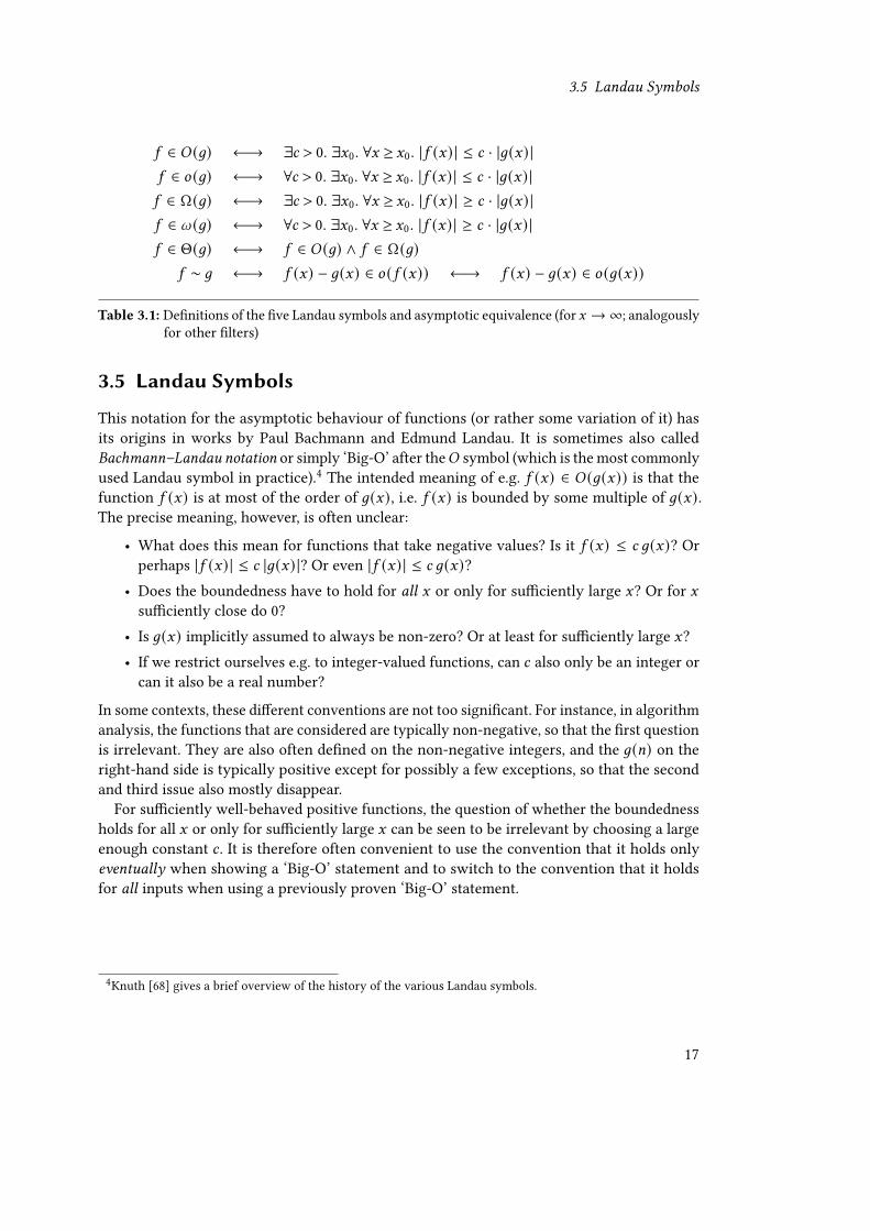
Table 3.1: Denitions of the ve Landau symbols and asymptotic equivalence (for 𝑥 →∞; analogouslyfor other lters)
3.5 Landau Symbols
This notation for the asymptotic behaviour of functions (or rather some variation of it) hasits origins in works by Paul Bachmann and Edmund Landau. It is sometimes also calledBachmann–Landau notation or simply ‘Big-O’ after the𝑂 symbol (which is themost commonlyused Landau symbol in practice).4 The intended meaning of e.g. 𝑓 (𝑥) ∈ 𝑂 (𝑔(𝑥)) is that thefunction 𝑓 (𝑥) is at most of the order of 𝑔(𝑥), i.e. 𝑓 (𝑥) is bounded by some multiple of 𝑔(𝑥).The precise meaning, however, is often unclear:
• What does this mean for functions that take negative values? Is it 𝑓 (𝑥) ≤ 𝑐 𝑔(𝑥)? Orperhaps |𝑓 (𝑥) | ≤ 𝑐 |𝑔(𝑥) |? Or even |𝑓 (𝑥) | ≤ 𝑐 𝑔(𝑥)?
• Does the boundedness have to hold for all 𝑥 or only for suciently large 𝑥? Or for 𝑥suciently close do 0?
• Is 𝑔(𝑥) implicitly assumed to always be non-zero? Or at least for suciently large 𝑥?• If we restrict ourselves e.g. to integer-valued functions, can 𝑐 also only be an integer orcan it also be a real number?
In some contexts, these dierent conventions are not too signicant. For instance, in algorithmanalysis, the functions that are considered are typically non-negative, so that the rst questionis irrelevant. They are also often dened on the non-negative integers, and the 𝑔(𝑛) on theright-hand side is typically positive except for possibly a few exceptions, so that the secondand third issue also mostly disappear.
For suciently well-behaved positive functions, the question of whether the boundednessholds for all 𝑥 or only for suciently large 𝑥 can be seen to be irrelevant by choosing a largeenough constant 𝑐 . It is therefore often convenient to use the convention that it holds onlyeventually when showing a ‘Big-O’ statement and to switch to the convention that it holdsfor all inputs when using a previously proven ‘Big-O’ statement.
4Knuth [68] gives a brief overview of the history of the various Landau symbols.
17

3 Preliminaries
In algorithm analysis, Landau symbols are usually used to study the behaviour of functionsfor 𝑥 → ∞. However, in mathematical analysis, the 𝑂 (. . .) symbol is also often used in thecontext of the local behaviour of real or complex functions. For instance, Taylor’s theorem fora function 𝑓 : R𝑚 → R𝑛 that is 𝑘-times dierentiable at 𝑥 is often written as
𝑓 (𝑥 + ℎ) = 𝑓 (𝑥) + 𝑓 ′(𝑥)ℎ + . . . + 𝑓(𝑘) (𝑥)𝑘! ℎ𝑘 + 𝑅(ℎ) where 𝑅(ℎ) ∈ 𝑂 (ℎ𝑘+1) ,
where the 𝑂 (. . .) implicitly contains the restriction ‘for suciently small ℎ.’5In the context of a theorem prover, a clear choice for the denition of 𝑂 (. . .) etc. must be
made once and for all. In Isabelle, the situation is now as follows: I dened ve Landau symbols,plus the related notion of asymptotic equivalence, written as 𝑓 (𝑥) ∼𝑔(𝑥). Their denitions canbe found in Table 3.1. These symbols were originally bundled in an AFP entry called LandauSymbols, but were later moved to the Isabelle distribution to allow using them also to aidproofs within the standard library.
When I designed these denitions at the beginning of my PhD project, I had to attempt tochoose one particular precise meaning while still allowing the user to use these symbols in aexible way in the wide variety of dierent contexts in which they are practically used. Sincethere are ve Landau symbols in total, the choices should also be uniform among all thesesymbols and make sense for all of them. In the end, I made the following decisions:
• No assumptions on zeroness or non-negativity of functions are made.• The absolute value (or rather the norm) is used in order to make the Landau symbolstruly scale-invariant in the sense that 𝑂 (𝑎𝑓 (𝑥)) and 𝑂 (𝑓 (𝑥)) are the same for anyconstant 𝑎 ≠ 0.
• 𝑐 can always be any positive real number.• The precise neighbourhood in which the boundedness should hold is 𝑥 →∞ by defaultbut can be adjusted with an additional argument.
To elaborate on the last point, the Isabelle/HOL library (like some libraries in other proofassistants) uses lters [64], a concept going back to Bourbaki, to denote topological conceptssuch as neighbourhoods and limits. These lters are very powerful and modular abstractionsfor such topological matters (and much more), but the details of how they are dened andhow they work are not relevant for this thesis. Let me only give these examples: the ‘at-top’lter corresponds to 𝑥 →∞ (i.e. the neighbourhood of∞ in a linear order), whereas the ‘at 𝑐’lter corresponds to the pointed neighbourhood of the point 𝑐 .This lter-centred approach to Landau symbols (which was suggested to me by Johannes
Hölzl) is very exible. For example, the following can be achieved:
• The abovementioned bound in Taylor’s theorem can be written as ‘𝑅(ℎ) ∈ 𝑂at 0(ℎ𝑘+1)’.5To complicate matters even more, both mathematicians and computer scientists often write terms such as𝑓 (𝑥) = 𝑒𝑥+𝑂 (1) where 𝑂 (1) implicitly stands for ‘some function that is 𝑂 (1).’ Enabling such notation in thecontext of a proof assistant is dicult, although there is work on this in Coq [1]. In some contexts, it is alreadypossible to write such things in Isabelle, but I for one do not make use of it.
18

3.5 Landau Symbols
• The alternative meaning of Landau symbols where the inequality must hold for allinputs can be achieved by using the ‘top’ lter, which represents the entire set of possibleinputs for the function (not to be confused with the ‘at-top’ lter).
• By using product lters, the Landau symbols can be used for multivariate functions aswell. This was done e.g. by Zhan and Haslbeck [103] to analyse algorithms taking morethan one input.
• Suppose we are analysing the sorting algorithm insertion sort, which sorts a given list𝑥 with 𝑛 elements, taking 𝑡 (𝑥) steps of time. It is well-known that 𝑡 (𝑥) ∈ 𝑂 (𝑛2) forsuciently large 𝑛, but it is not immediately clear how to capture this formally sincethe left-hand side is in terms of the list 𝑥 , not its size 𝑛. Clearly, the intended meaningis somehow that this holds for all lists of size 𝑛 for any suciently large 𝑛. In Isabelle,one can actually easily achieve exactly this meaning by writing
𝑡 (𝑥) ∈ 𝑂 length going-to at-top(length(𝑥)2) ,
with the ‘going-to’ lter stating that the intended asymptotic meaning is that it is thelength of the input that must be suciently large.
• Lastly, Stirling’s formula for the complex-valued Γ function states that
Γ(𝑧) ∼√
2𝜋𝑧
(𝑧𝑒
)𝑧uniformly as |𝑧 | → ∞ but only if 𝑧 lies within the cone |arg(𝑧) | ≤ 𝛼 for a xed angle𝛼 < 𝜋 . We can write this in Isabelle by annotating the ∼ with the lter
at-innity u principal (complex-cone (−𝛼) 𝛼)
where u denotes the greatest lower bound of two lters (the intersection, in a sense).
This illustrates how widely usable and exible Isabelle’s Landau symbols are.
19

4 Summary of Contributions
The overall theme of the work presented here is the formalisation of mathematics in a proofassistant (or interactive theorem prover), with a particular focus on asymptotic properties. Iused the aforementioned Isabelle/HOL as the underlying system, but the work could just aswell be replicated in any proof assistant that uses some form of classical logic suitable to theformalisation of standard mathematics. In the following, I will give a very brief and high-leveloverview of the work presented in the four publications that form this publication-based dis-sertation – more detailed summaries and background can be found in the remaining chapters.
Semi-Automatic Real Asymptotics [39]. This publication presents an automatic proofprocedure very much in the spirit of the series expansion procedures implemented in com-puter algebra systems. It facilitates reasoning about limits and other asymptotic properties ofconcrete real-valued functions. A large class of functions is covered (combinations of basicarithmetic, exp, log, sin, etc.).
Divide-and-Conquer Recurrences [30]. Here, I describe the rst formalisation of theAkra–Bazzi Theorem on the asymptotics of divide-and-conquer recurrences. It is a generalisa-tion of the well-known Master Theorem. These recurrences often arise in the asymptotic run-ning time analysis of divide-and-conquer algorithms. Such algorithms (including e.g. MergeSort and Karatsuba multiplication) and their analysis are a staple of undergraduate algorithmscourses and textbooks (see e.g. Cormen et al. [25]) and are of great practical importance aswell. The precise solutions to such recurrences are typically very complicated and can oftennot be expressed in a closed form, but the classic Master Theorem and the Akra–Bazzi The-orem provide a ‘cookbook method’ to determine their asymptotic growth relatively easily. Inaddition to the formalisation of the theorem itself, some automation infrastructure is providedin order to facilitate applying the theorem to concrete examples.
Linear Recurrences [40]. In contrast to divide-and-conquer recurrences, linear recurrences(with constant coecients) are a class of recurrence relations for which the exact solutionshave a very simple form and can be determined fairly easily. This work describes the (probably)rst formalisation of the theory of these recurrences (both homogeneous and inhomogeneous)and an executable solver for them. However, the exact solutions can contain irrational algeb-raic numbers, which are dicult to handle. For the use case where one is only interested inasymptotic upper bounds of the solution, I therefore also implemented a certifying approachthat uses ideas from analytic combinatorics and tools from complex analysis to prove ‘Big-O’ bounds. The exact solver relies on a formalisation of executable algebraic numbers byThiemann et al. [94] and the certier relies on a formalisation of executable complex-rootcounting by Li et al. [73]
21
4 Summary of Contributions
Analytic Number Theory [29]. This is by far the largest individual formalisation workpresented in this thesis: a formalisation of most chapters of Apostol’s classic textbook Introduc-tion to Analytic Number Theory. Analytic number theory arose in the mid-19th century in thestudy of the distribution of prime numbers, and this is still the application that it is best knownfor. Its most famous theorems are the Prime Number Theorem (on the asymptotic distributionof primes) and Dirichlet’s Theorem (on the innitude of primes in arithmetic progressions),and its most important tools are Dirichlet series and the Riemann Z function. All of this (andmuch more) is covered in Apostol’s book and was formalised by me as part of this work.
Related Contributions Without Formal Publications. In addition to the four articlesthat were just mentioned, I also have other contributions to the Isabelle/HOL distribution andthe Archive of Formal Proofs that are not part of any formal publication. I would like to brieymention some that are related to this thesis because they are either directly used by the otherwork described in it or also concern the subject of asymptotics.
In the Isabelle distribution, there are:
• the Γ function• the radius of convergence of a power series and various summability tests• the generalised binomial theorem• the connection between formal power series and complex functions
The last item here is particularly signicant since a similar connection between a class offormal series and analytic functions will also appear in my work on analytic number theoryin Chapter 8.
As for the Archive of Formal Proofs, I specically have entries on:
• Stirling’s formula (the asymptotics of 𝑛! and Γ) [31]• Catalan numbers, including an analytic-combinatorics-inspired derivation of their asymp-totics [26]
• basic properties of some special functions like the error function and the Lambert𝑊function, including their asymptotic behaviour [32, 36]
• the Euler–MacLaurin formula (relating sums to integrals) [33]• advanced properties of Bernoulli numbers (building on work by Bulwahn) [18]
The last two items again play an important role in analytic number theory, specically inconnection with the Hurwitz and Riemann Z functions.
22

5 Semi-Automatic Real Asymptotics
“ Divergente Rækker ere i det Hele noget Fandensskab,og det er en Skam at man vover at grunde nogen Démonstration derpaa.Man kan faae frem hvad man vil naar man bruger dem,og det er dem som har gjort saa megen Ulykke og saa mange Paradoxer.
Divergent series are, all in all, an abomination,and it is shameful that one should dare base any proof upon them.Using them, one can obtain whatever one wishesand they have created so much misfortune and so many paradoxes.
— Niels Henrik Abel, in a letter to Bernt Holmboe (1826) ”“ The series is divergent;
therefore we may be able to do something with it.— attributed to Oliver Heaviside ”
It is not surprising that when formalising mathematics with a proof assistant, one frequentlyhas to prove limits and other asymptotic properties of concrete functions. On the simple endof the spectrum, there are e.g.
lim𝑛→∞(𝑛 + 𝑐) lim
𝑛→∞𝑛
𝑛2 + 1 𝑐 𝑥𝑛 ∈ 𝑂 (𝑒𝑥 ) ,
which a human mathematician would regard as completely trivial. On the other hand, thereare problems such as
log𝑛 𝑘𝑘− 1𝑛 + 1
(log𝑛+1(𝑘 + 1) − log𝑛+1 𝑘 ) ∼ 1
2𝑘−2 log𝑛 𝑘 for 𝑘 →∞
lim𝑥→∞
(1 − 1
𝑏 log1+Y 𝑥
)𝑝 (1 + 1
logY/2(𝑏𝑥 + 𝑥 log−1−Y 𝑥 )
)−
(1 + 1
logY/2 𝑥
)= ?
which are fairly tedious to do even on paper.
Recall that log𝑘 𝑥 means (log𝑥)𝑘 , not the iterated logarithm.
Unfortunately, in my personal experience, all of these are tedious to do in a theorem prover.The ones that are easy on paper tend to be easier in the theorem prover as well, but still: even
23
5 Semi-Automatic Real Asymptotics
for one of the trivial problems listed above, one might need a few lines of formal proofs andremember the names of all the required library theorems. Since such simple problems tendto arise very often, this eort accumulates and becomes quite cumbersome in any seriousmathematical formalisation project involving asymptotic arguments. As for the more dicultproblems, my rst version of the formal proof of the last example above required 700 linesof formal proofs and more than a week of time (see the attached article in Chapter B in theappendix).On the other hand, unveried symbolic computer algebra systems such as Mathemat-
ica [102] or Maple [97] have been solving such problems fairly well since the 1990s. Thepainful experience of having to prove asymptotic statements like the ones above over andover again caused me to look into how modern computer algebra systems solve such prob-lems. This brought me to the work by Gruntz [50], which ultimately led me to the Multiseriesexpansions by Shackell et al. [87].
The nal outcome of my work in this area was then a proof-constructing procedure1 thatcan compute Multiseries expansions for a wide variety of real-valued functions, from whichthe desired asymptotic properties of the function (such as limits or ‘Big-O’ behaviour) canthen be read o. I called the procedure semi-automatic because it relies on Isabelle’s existingautomation to solve the question of whether a given expression is or is not equal to zero,and if it is not, whether it is positive or negative. When this automation fails, the user muststep in and supply additional facts until the automation can deduce this information. In myexperience, this does not happen particularly often in practice.
This procedure has since become invaluable to me in automating both the abovementionedmultitude of trivial asymptotic problems and themore dicult problems that arise occasionally.In particular, it facilitates working with integrals or innite sums: rigorous formal proofsrequire establishing integrability or summability explicitly, and this can often be done mosteasily by performing a comparison test with a suitable ‘Big-O’ bound.For example, the rst of the last two examples given above arises in proving the well-
denedness of the Stieltjes constants (the Laurent series coecients of Z (𝑠) at 𝑠 → 1). Theseare dened as an innite sum whose convergence is most easily shown by noting that thesummand is 𝑂 (𝑘−1.5), and 𝑘−1.5 is clearly summable. This ‘Big-O’ estimate involves cancella-tion, so it would have been quite tedious to prove by hand in Isabelle, whereas the automationcan now do it easily.
The other of the two examples arose in the formalisation of the Akra–Bazzi theorem (whichwill be covered in Chapter 6). As mentioned above, the rst, manual proof for this limit wasover 700 lines long and took over a week to write (not counting quite some time before that tounderstand how to even prove it rigorously on paper). This experience was in fact my originalmotivation for creating real_asymp – which can now prove it fully automatically in lessthan a second.
1‘Proof-constructing’ means that the procedure builds an actual proof by (at the end of the day) interacting withthe Isabelle kernel, as opposed to acting as or using some kind of oracle (such as computational reection).This means that it can also construct a proof object, although this is usually not enabled in Isabelle. In principle,this does however open up the possibility of replaying such proofs in other theorem provers.
24
5.1 Multiseries
5.1 Multiseries
The basic tool upon which real_asymp is based is the concept of Multiseries. A Multiseriesis a formal power series in 𝑛 variables, with real coecients and exponents. The variablesthemselves are functions 𝑏1(𝑥), . . . , 𝑏𝑛 (𝑥) of a real variable 𝑥 . Consequently, the monomialsof a Multiseries are of the form 𝑐 𝑏1(𝑥)𝑒1 . . . 𝑏𝑛 (𝑥)𝑒𝑛 . The vector of these 𝑛 functions is calledan asymptotic basis.By convention, we always consider series at the point 𝑥 →∞. The functions in an asymp-
totic basis are also, by convention, required to tend to ∞ as 𝑥 → ∞. Furthermore, they aresorted descendingly by growth in the sense that log𝑏𝑖+1(𝑥) ∈ 𝑜 (log𝑏𝑖 (𝑥)). This implies, inparticular, that 𝑏𝑖 (𝑥)Y grows faster than 𝑏𝑖+1(𝑥)𝑒 for any Y > 0 and any 𝑒 . Due to this, asymp-totic comparisons of monomials are very easy: comparing the growth of two monomials isequivalent to comparing their exponent vectors lexicographically.The following sections will give a brief informal explanation of Multiseries with the aim
to convey the general picture. More detailed information on these theoretical aspects can befound in the works of Richardson et al. [87], Shackell [90], and Van der Hoeven [62].
Formal Definition
Formally, Multiseries can be seen simply as a function from exponent vectors to coecients,i.e. R𝑛 → R. However, additional restrictions on the support of this function must be made. Inour setting, we will always deal with Multiseries with nitely-generated support, i.e. whosesupport is contained in a set of the form
𝛼 + _1𝛽1 + . . . + _𝑘𝛽𝑘 | _𝑖 ∈ N for xed vectors 𝛼 ∈ R𝑛 and 𝛽1, . . . , 𝛽𝑘 ∈ R𝑛≤0.
This formal view is, however, not particularly useful for implementation purposes. Since theend goal is not to have a nice algebraic formalisation of Multiseries but rather to have apractical tool for asymptotic reasoning, the Isabelle formalisation does not dene Multiseriesthis way. Rather, it follows the same approach that is used in the Maple implementation bySalvy [97], which uses a more application-driven hierarchical denition. I will now explainwhat this representation looks like.
Representation
Let us rst consider ‘normal’ generalised power series – that is, power series in one variable𝑥 where exponents can be any real number. These are essentially Multiseries with only onebasis element, which is 𝑥 . Under reasonable support conditions, they can be thought of andrepresented as a linear sequence of coecients and exponents, where the exponents arerequired to decrease strictly. For instance, the power series expansion of 𝑒1/𝑥 at 𝑥 → ∞ canbe represented as the sequence 1 + 𝑥−1 + 1
2𝑥−2 + . . .
In a functional setting, the obvious representation of such a series is simply a (possiblyinnite) list of pairs of real numbers (coecient and exponent). In Isabelle/HOL, that typewould be written as (real × real) llist (since possibly-innite lists are called ‘lazy lists’ infunctional programming).
25

5 Semi-Automatic Real Asymptotics
1𝑥−1 · exp(𝑥)0 + 1 · exp(𝑥)−1 + 1 · exp(𝑥)−2 + . . .
1 · 𝑥0 1 · 𝑥0
1 · 𝑥−1 + 1 · 𝑥−2 + 1 · 𝑥−3 + 1 · 𝑥−4 + . . .
Figure 5.1: A hierarchical illustration of the Multiseries of the function 1𝑒𝑥−1 + 1
𝑥−1 for 𝑥 → ∞ w.r.t.the basis 𝑏1 (𝑥) = exp(𝑥) and 𝑏2 (𝑥) = 𝑥 .The uppermost layer (represented by a double rectangle) is a power series in 𝑏1. Its coef-cients are again Multiseries w.r.t. the singleton basis 𝑏2, which are represented by theother rectangles below. The circled digits ‘1’ in the in the single-framed rectangles are thensimply Multiseries w.r.t. the empty basis (i.e. constants).
For Multiseries, this simple linear representation is usually not possible. Consider the fol-lowing example:
1𝑥 − 1 +
1𝑒𝑥 − 1 ∼
∞∑𝑖=1
𝑥−𝑖 +∞∑𝑖=1
exp(𝑥)−𝑖
The function on the left-hand side has the Multiseries expansion on the right-hand side at𝑥 →∞. This series is a innite sequence of monomials of the form 𝑥−𝑖 , followed by an innitesequence of monomials of the form exp(𝑥)−𝑖 . If we implemented the series as simply a lazylist of monomials, the information on the second term would be completely lost: if we were tosubtract 1
𝑥−1 from our series, we should be able to nd that the leading term is now exp(𝑥)−1– but with the linear representation, we would be left with nothing but an innite number ofzero terms.In general, it is even possible to have e.g. an innite sequence of innite sequences of
monomials. To accommodate this more intricate structure, one can adopt a hierarchical view:
• A Multiseries with an empty basis is just a single real number.• A Multiseries with a basis 𝑏1, . . . , 𝑏𝑛 is a generalised power series in 𝑏1(𝑥) whose coe-cients are Multiseries with the basis 𝑏2, . . . , 𝑏𝑛 .
The following pseudocode illustrates roughly how Multiseries are dened in Isabelle/HOL:
[] multiseries = real[𝑏1, . . . , 𝑏𝑛] multiseries = ( [𝑏2, . . . , 𝑏𝑛] multiseries × real) llist
Figure 5.1 illustrates this principle on our earlier example. The list of the innitely manymonomials 𝑥−𝑖 together forms the rst monomial of the overall Multiseries, and each of themonomials exp(𝑥)−𝑖 is another monomial after that. Thus, all the asymptotic information ispreserved: if we were to subtract 1
𝑥−1 from this series, the rst monomial of the Multiserieswould disappear and the new leading term would be exp(𝑥)−1, as it should be.
26

5.1 Multiseries
Connecting Series and Functions
Although Multiseries are convergent in many cases, they can be divergent2 (cf. e.g. Stirling’sformula for the Γ function). This means that looking at a particular Multiseries, it is not alwaysimmediately obvious which actual real function (if any) it corresponds to.
However, in our case, we are only interested in attaching a Multiseries to a known function,which can be done in analogy to Poincaré series. For this purpose, let us rst again considerthe easier setting of ‘normal’ power series where we only have one basis element 𝑥 . For afunction 𝑓 : R→ R and such a series,
𝑓 (𝑥) ∼∞∑𝑖=0
𝑐𝑖𝑥𝑒𝑖
holds in the sense of a Poincaré expansion i(𝑓 (𝑥) −
𝑁∑𝑖=0
𝑐𝑖𝑥𝑒𝑖
)∈ 𝑜 (𝑥𝑒𝑖 ) for all 𝑁 ∈ N .
A nice alternative coalgebraic formulation of this is the following inference rule:
𝑓 (𝑥) ∈ 𝑂 (𝑥𝑒0
)𝑓 (𝑥) − 𝑐0𝑥𝑒0 ∼ ∑∞
𝑖=0 𝑐𝑖+1𝑥𝑒𝑖+1
𝑓 (𝑥) ∼ ∑∞𝑖=0 𝑐𝑖𝑥
𝑒𝑖
If we interpret this inference rule as the denition of a coinductive relation ∼, we obtainexactly the same predicate as with the Poincaré denition, but can use corecursion to reasonabout it. For instance, the correctness lemmas for operations on series become straightforwardcoinduction proofs.A very similar inference rule can be used to dene a ∼ relation on Multiseries. The main
dierence is that since the coecients are then again Multiseries (with a smaller basis), thesealso need to recursively satisfy the ∼ relation for the functions that they represent.
The Anatomy of the Basis Functions
Let us now turn to what form the asymptotic bases have concretely. In our setting, everybasis always contains the function 𝑥 . After this 𝑥 , we can have a list of increasingly iteratedlogarithms of 𝑥 . Before the 𝑥 , we can have exponentials of functions that already have anexpansionw.r.t. the smaller basis elements after it. For the purpose of illustration, the followingis a valid asymptotic basis:
exp(exp(𝑥2) + exp(√𝑥)), exp(𝑥2 − 𝑥), exp(𝑥), exp(√𝑥),𝑥, log𝑥, log log𝑥, log log log𝑥
2In case the reader now feels some unease concerning the earlier quotation by Abel, they need not worry. Abelwas referring to unsound manipulation of divergent series. No such issues arise in our context, and even ifthey did, the theorem prover would force us to handle them in a sound way.
27
5 Semi-Automatic Real Asymptotics
This approach is sucient to treat a wide variety of functions, including everything built from
• basic arithmetic• exponentials, logarithms, roots• the ‘absolute value’ and sgn functions• the trigonometric functions sin, cos, tan as long as their argument does not tend to∞• arctan, Γ (the Gamma function),𝜓 (the Polygamma functions), erf (the error function),Bessel functions, the Riemann Z function3
This can also be extended to other classes of functions (such as implicit functions, inversefunctions, and solutions of dierential equations [90]) but that is certainly beyond the scopeof the present work.
5.2 Implementation
Shackell et al. [87] sketch a bottom-up syntax-directed procedure to produce Multiseriesexpansions for a real-valued function that is given as an explicit expression. The basis of theMultiseries is computed on-the-y, starting with the basis 𝑥 and adding new basis elementsas needed.The Isabelle implementation of real_asymp follows exactly this approach. Of course,
the traditional implementation of the algorithm by Shackell et al. is in the context of a com-puter algebra system, where only a result has to be produced. Since we are working in atheorem prover, we must produce theorems in every step. real_asymp must prove the well-formedness of all the asymptotic bases and Multiseries it produces, and that the Multiseries isindeed an expansion for the given function. To do this, an Isabelle/HOL function was denedand proven correct for each of the operations in the syntax-directed procedure (under somesuitable preconditions). The actual real_asymp procedure then only has to
• construct the Multiseries for the function expression bottom-up,• plug the correctness results of the relevant operations together,• prove the arising preconditions (which are often of the form ‘this real-number term isnon-zero’ or ‘this real-number term is greater than 1’),
• evaluate the resulting Multiseries as far as needed (usually until the leading term canbe read o),
• interpret the result (e.g. if the leading term is of the form 𝑐 (𝑥)𝑏1(𝑥)𝑒 with 𝑒 < 0, weknow that the function tends to 0).
This approach naturally leads to a proof-producing procedure: every step of the reasoningdone by real_asymp passes through the Isabelle kernel.The evaluation of the Multiseries requires a way to lazily expand equational denitions
until a certain point, which is why real_asymp contains a simple ad-hoc proof-producingengine for lazy evaluation of Isabelle/HOL terms. Since the evaluation must produce Isabelle3Of these special functions, only arctan, Γ, and erf were implemented in real_asymp, and only partially.
28

5.3 Asymptotic Interval Arithmetic
theorems, there is signicant performance overhead in this step compared to e.g. a computeralgebra system. Sharing of common subexpressions is currently also not supported, since thecombination of sharing and producing theorems is not straightforward.One problematic aspect of the entire implementation is the aforementioned determina-
tion of signs and zeroness. Even for constants built from a fairly restricted set of operations,determining zeroness is not known to be decidable. For the most basic setting of exp–log func-tions, Richardson [86] gave a partially correct algorithm whose termination is contingent onSchanuel’s conjecture, a deep conjecture in transcendental number theory. In the considerablymore liberal setting that we have, zero equivalence (and thus also sign determination) areknown to be undecidable due to another theorem by Richardson [85]. Due to the complexityof the problem, the real_asymp procedure simply uses Isabelle’s simplier and optionallyIsabelle’s approximation package [63] as heuristics to solve such problems, and fails if itis unable to determine the signs that way. This is in line with what computer algebra tools do:Maple, for instance, uses a number of heuristic and probabilistic methods to determine if anexpression is zero but does not implement anything along the lines of Richardson’s algorithm.4
5.3 Asymptotic Interval Arithmetic
Oscillating functions such as sin(𝑥) or b𝑥c for 𝑥 →∞ do not have Multiseries expansions sothat the approach as presented above does not work for them. Generalising the Multiseriesframework to encompass such functions is dicult; some approaches exist (e.g. measuredlimits by Salvy and Shackell [89]) but are probably too complicated to justify the additionalcomplexity for an application such as ours. I therefore implemented another fairly straight-forward approach that builds on top of Multiseries in a modular way: when real_asympencounters a possibly oscillating expression (such as sin(𝑓 (𝑥)) or b𝑓 (𝑥)c where 𝑓 (𝑥) doesnot tend to a nite value), it uses reasonable asymptotic lower and upper bounds (e.g. −1 and1 resp. 𝑓 (𝑥) − 1 and 𝑓 (𝑥) in the previous two examples). This requires implementing a kindof interval-arithmetic approach for asymptotic expansions, i.e. all the dierent cases in thesyntax-directed procedure mentioned previously now need to be modied to handle the caseswhere the input is not just a function with a single Multiseries expansion but possibly onewith an asymptotic lower and upper bound, each having a separate Multiseries expansion.This adds a considerable amount of implementation eort.
This approach is certainly not complete since the usual problem of interval arithmetic occurs:wrapping. For a drastic example, consider the function sin(𝑥) − sin(𝑥). Since real_asympdoes not simplify the input term, it infers the bounds [−1, 1] for each of the sin(𝑥) terms,leading to an overall result of [−2, 2] instead of just 0. A less obvious example would besin(𝑥) + cos(𝑥) with the inferred bounds [−2, 2] while the best possible bounds are [−√2,√2].However, this approach can still handle many practical examples – in particular, it is veryuseful in gauging the asymptotic error made by rounding, such as
√b𝑥c = √𝑥 +𝑂 ( 1√
𝑥
).
4according to an answer on Math StackExchange by Jacques Carette, a former Maple developer (https://math.stackexchange.com/questions/3606561)
29

5 Semi-Automatic Real Asymptotics
5.4 Related Literature
There is little other work on automating proofs for asymptotic statements in a theorem prover.Avigad and Donnelly [6] developed a decision procedure for the fragment of linear Big-Oexpressions (which has unfortunately never been integrated into a theorem prover).
In my publication on the Akra–Bazzi theorem [30], I developed some simple, more heuristicautomation for Landau Symbols (see Chapter 6 for more details on this).Publications on formalisation techniques for asymptotics are also relatively rare. Hölzl et
al. [64] describe how Isabelle/HOL uses lters to denote and reason about limits and otherasymptotic properties (which is also heavily used in my work). Harrison [59] describes the useof nets for the same purpose in HOL Light. Aeldt et al. [1] describe a formalisation approachfor ‘Big-O’-style asymptotics in Coq, including some tactics to facilitate making assumptionssuch as ‘𝑥 is big enough’ in an idiomatic way.Outside the realm of theorem proving, the most relevant literature that I am aware of are
the aforementioned article by Shackell et al. [87] and dissertation by Gruntz [50], and, fora more comprehensive view on the matter, a book by Shackell [90]. There is also a book byVan der Hoeven [62], which takes the somewhat dierent route of Transseries, but I found theMultiseries approach from the previously mentioned sources more accessible for my purposes.
5.5 Future Work and Outlook
There are still some minor issues with the current version of real_asymp that shouldeventually be remedied:
• Sometimes, the expressions arising in intermediate steps become so complicated thatthe simplier is no longer able to recognise them as zero. It is not clear if and how thiscan be avoided.
• While there is a limited plugin system to add support for new special functions at the‘user level’, doing so is currently very tedious and only done for the Γ function as aproof of concept.
• The functions exp, log, sin, etc. all satisfy nice equations w.r.t. addition and/or multiplic-ation, which makes deriving Multiseries expansions for them fairly easy. For functionssuch as Γ and arctan, the situation is more complicated and the support for these istherefore still incomplete. Shackell [90] briey explains how to handle this case, butwithout giving a proof. I was not able to nd an actual proof of this anywhere else in theliterature either. Moreover, it would unfortunately be dicult to integrate that approachwith the current setting of real_asymp on a purely technical level as well.
When I spent more time formalising mathematics after the development of real_asymp,I also came across the following more ‘high-level’ ideas for future work:
• In exactly the same way as real_asymp, one could write a procedure to determineLaurent series expansions for meromorphic complex functions. In fact, the implement-ation would actually be signicantly more straightforward since Laurent series areconceptually much simpler than Multiseries seeing as there is no ‘asymptotic basis’ –
30

5.5 Future Work and Outlook
just integral powers of 𝑥 . Such a method could automate some of the tedious tasks thatarise when doing complex analysis in Isabelle, such as limits, pole cancellation, anddetermination of residues.
• It would be desirable for real_asymp to also work with partial asymptotic informa-tion, e.g. the user could prove that 𝑓 (𝑥) = 𝑥 +𝑂 (1) and then ask for the limit of 𝑒 𝑓 (𝑥) .This would, however, require a full rewrite of much of the existing code, and it is notquite clear how this would interact with the existing ‘asymptotic interval arithmetic’.
The rst item in particular seems very promising, since it would probably be comparativelylittle work and result in a very useful tool that could, among other things, simplify some ofthe complex-asymptotic reasoning in mywork on the formalisation of analytic number theory.
Looking at other systems than Isabelle/HOL, it should be noted that the mathematicalprerequisites of real_asymp are very moderate: limits (of course), convergent power series,Landau symbols, and ideally a framework for coalgebraic denitions and reasoning. Theformalisation behindreal_asymp itself is also relatively small and consists entirely of simpleand straightforward proofs. It should therefore be possible to implement a similar procedurein any system with a library of classical analysis (such as Coq, Lean, or HOL Light) with littleformalisation eort. However, the implementation eort was very substantial in Isabelle andmay well be so in other systems as well.
31

6 Divide-and-Conquer Recurrences
“ Entzwey’ und gebiete! Tüchtig Wort:Verein’ und leite! Beßrer Hort.
Divide and Conquer! Fine words.Unite and lead! A better tenet.
— Johann Wolfgang von Goethe (1814)”The famousMaster Theorem is part of any undergraduate lecture on algorithms. It can be usedfor the running time analysis of a large class of classic divide-and-conquer algorithms, whichhave the following form:
Input: A problem of size 𝑛Algorithm: For 𝑛 suciently small, solve non-recursively. Otherwise:
1. split the problem into𝑚 subproblems of size 𝑛/𝑘2. solve each problem recursively3. combine the𝑚 subsolutions into a solution for the original problem
If we denote the time required by this algorithm with𝑇 (𝑛) and the time required to recombinethe solutions in the last step of each recursion with 𝑔(𝑛), this gives us the recurrence
𝑇 (𝑛) =𝑚 ·𝑇 (𝑛/𝑘) + 𝑔(𝑛)
for suciently large 𝑛. The Master Theorem allows us to determine the asymptotic growth of𝑇 (𝑛) in this setting under some mild conditions. The upper half of Table 6.1 lists some notableexample applications of the Master Theorem.The theorem was introduced by Bentley et al. [10] in 1980. Cormen et al. popularised it
under the name Master Theorem in their famous textbook. For reasons that will be discussedin the next section, I instead formalised a generalisation by Akra and Bazzi [2] from 1998 thatapplies to more general recurrences (such as the ones in the lower half of Table 6.1).
6.1 The Formalised Theorem
My original plan was to formalise the Master Theorem, but the proofs found in textbooksseemed less than ideal for formalisation. The Master Theorem is divided into three dierentcases that are proven completely separately. Additionally, due to the discrete nature of theinputs, algorithms cannot always evenly divide subproblems in practice – for instance, theMerge Sort recurrence is not really 𝑇 (𝑛) = 2𝑇 (𝑛/2) + 𝑂 (𝑛), but rather 𝑇 (𝑛) = 𝑇 (b𝑛/2c) +
33

6 Divide-and-Conquer Recurrences
Algorithm Recurrence Asymptotics
Binary search 𝑇 (𝑛) = 𝑇 (𝑛/2) +𝑂 (1) Θ(log𝑛)Merge Sort 𝑇 (𝑛) = 2𝑇 (𝑛/2) +𝑂 (𝑛) Θ(𝑛 log𝑛)Karatsuba multiplication 𝑇 (𝑛) = 3𝑇 (𝑛/2) +𝑂 (𝑛) Θ(𝑛log2 3)Ham-Sandwich trees 𝑇 (𝑛) = 𝑇 (𝑛/2) +𝑇 (𝑛/4) + 1 Θ(𝑛log2(1+
√5)−1)
Median-of-medians 𝑇 (𝑛) = 𝑇 (2/10 · 𝑛) +𝑇 (7/10 · 𝑛 + 6) +𝑂 (𝑛) Θ(𝑛)
Table 6.1: Three divide-and-conquer recurrences related to algorithm analysis with their asymptoticsas given by the Master Theorem, and two for which the Master Theorem does not apply(but the Akra–Bazzi Theorem does).
𝑇 (d𝑛/2e) +𝑂 (𝑛). This rounding introduces additional diculties and makes it impossible tond an exact closed-form solution inmost cases (even though it does not change the asymptoticresult at all). In informal presentations on paper, this aspect is often either ignored completelyor handled through additional case distinctions, which blows up the proof size even more.From my own formalisation experience, I felt that a more unied and high-level approach
would be easier to formalise, and it was this that led me to the Akra–Bazzi theorem. Thistheorem provides one single unied solution (albeit a more complex one) with no case dis-tinctions, and it solves the issue of rounding by allowing the recursive calls to have arbitrary‘error terms’ as long as they are small enough. This allows not only rounding up and down,but also adding arbitrary constants, or even terms such as b𝑛/2 + √𝑛c. It also generalises theMaster Theorem in another way, namely that the subproblems are not required to all havethe same size.My formalisation follows the presentation by Leighton [72], which generalises the result
by Akra and Bazzi even further and also provides a more elementary proof that seemed moresuitable for formalisation since the mathematical prerequisites for it are minimal.The precise class of recurrences that the Akra–Bazzi theorem, as presented by Leighton,
applies to is the following:
𝑇 (𝑛) = 𝑔(𝑛) +𝑚∑𝑖=1
𝑎𝑖 ·𝑇 (𝑏𝑖𝑛 + ℎ𝑖 (𝑛)) (6.1)
with 𝑎𝑖 ≥ 0 and 𝑏𝑖 ∈ (0, 1). Additionally, the recombination cost function 𝑔(𝑛) and the errorterms ℎ𝑖 (𝑛) need to satisfy some mild growth conditions. The resulting growth estimate is
𝑇 (𝑛) ∈ Θ(𝑥𝑝
(1 +
∫ 𝑥
𝑥0
𝑔(𝑢)𝑥𝑝+1
d𝑢))
where 𝑝 is the unique real solution of∑𝑎𝑖𝑏
𝑝
𝑖= 1. This rather unwieldy result can be simplied
signicantly for more concrete forms of 𝑔(𝑛) that often arise in practice, which then leads toa number of simple corollaries that have a form that is very similar to the standard MasterTheorem, but more general (see Table 6.2).
34
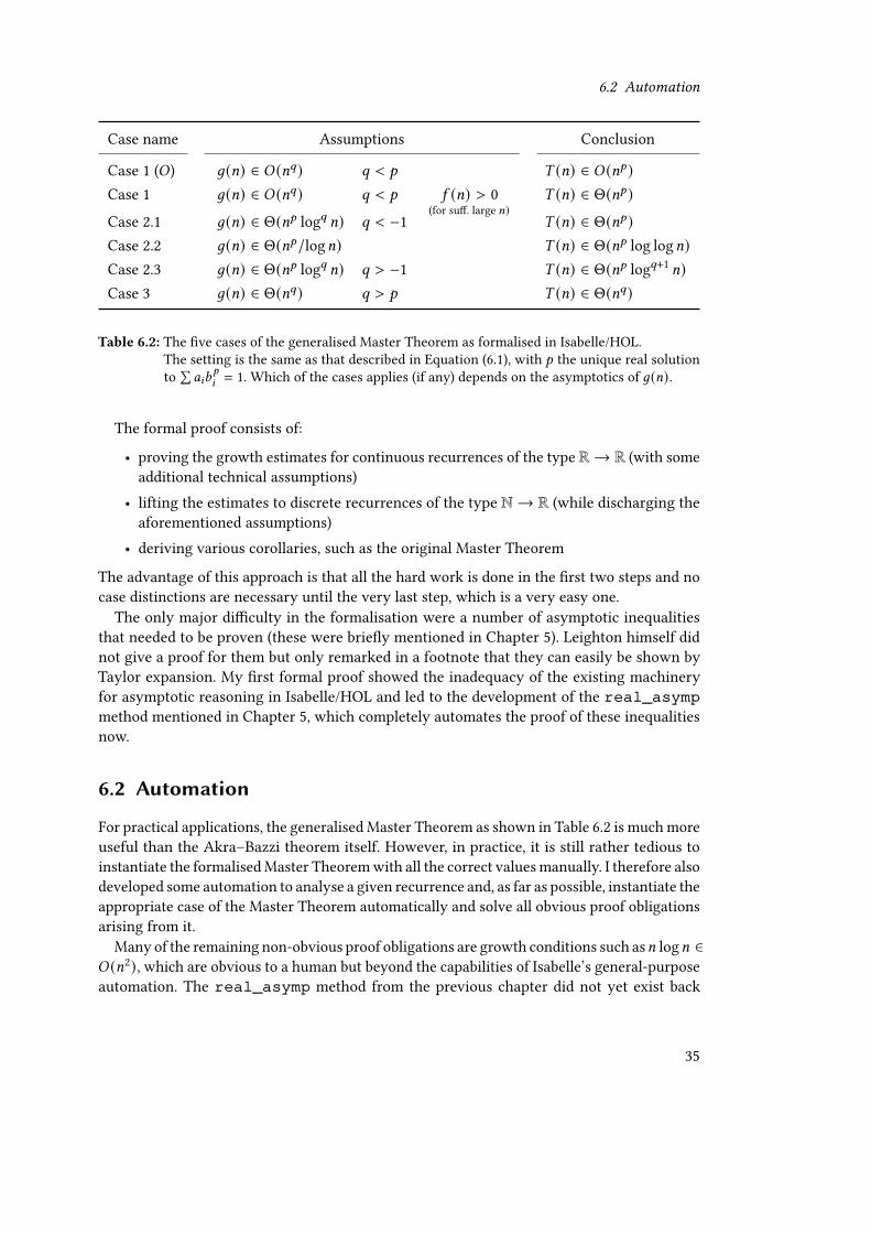
6.2 Automation
Case name Assumptions Conclusion
Case 1 (𝑂) 𝑔(𝑛) ∈ 𝑂 (𝑛𝑞) 𝑞 < 𝑝 𝑇 (𝑛) ∈ 𝑂 (𝑛𝑝)Case 1 𝑔(𝑛) ∈ 𝑂 (𝑛𝑞) 𝑞 < 𝑝 𝑓 (𝑛) > 0
(for su. large 𝑛)𝑇 (𝑛) ∈ Θ(𝑛𝑝)
Case 2.1 𝑔(𝑛) ∈ Θ(𝑛𝑝 log𝑞 𝑛) 𝑞 < −1 𝑇 (𝑛) ∈ Θ(𝑛𝑝)Case 2.2 𝑔(𝑛) ∈ Θ(𝑛𝑝/log𝑛) 𝑇 (𝑛) ∈ Θ(𝑛𝑝 log log𝑛)Case 2.3 𝑔(𝑛) ∈ Θ(𝑛𝑝 log𝑞 𝑛) 𝑞 > −1 𝑇 (𝑛) ∈ Θ(𝑛𝑝 log𝑞+1 𝑛)Case 3 𝑔(𝑛) ∈ Θ(𝑛𝑞) 𝑞 > 𝑝 𝑇 (𝑛) ∈ Θ(𝑛𝑞)
Table 6.2: The ve cases of the generalised Master Theorem as formalised in Isabelle/HOL.The setting is the same as that described in Equation (6.1), with 𝑝 the unique real solutionto
∑𝑎𝑖𝑏
𝑝
𝑖= 1. Which of the cases applies (if any) depends on the asymptotics of 𝑔(𝑛).
The formal proof consists of:
• proving the growth estimates for continuous recurrences of the type R→ R (with someadditional technical assumptions)
• lifting the estimates to discrete recurrences of the type N→ R (while discharging theaforementioned assumptions)
• deriving various corollaries, such as the original Master Theorem
The advantage of this approach is that all the hard work is done in the rst two steps and nocase distinctions are necessary until the very last step, which is a very easy one.The only major diculty in the formalisation were a number of asymptotic inequalities
that needed to be proven (these were briey mentioned in Chapter 5). Leighton himself didnot give a proof for them but only remarked in a footnote that they can easily be shown byTaylor expansion. My rst formal proof showed the inadequacy of the existing machineryfor asymptotic reasoning in Isabelle/HOL and led to the development of the real_asympmethod mentioned in Chapter 5, which completely automates the proof of these inequalitiesnow.
6.2 Automation
For practical applications, the generalised Master Theorem as shown in Table 6.2 is much moreuseful than the Akra–Bazzi theorem itself. However, in practice, it is still rather tedious toinstantiate the formalisedMaster Theoremwith all the correct valuesmanually. I therefore alsodeveloped some automation to analyse a given recurrence and, as far as possible, instantiate theappropriate case of the Master Theorem automatically and solve all obvious proof obligationsarising from it.
Many of the remaining non-obvious proof obligations are growth conditions such as𝑛 log𝑛 ∈𝑂 (𝑛2), which are obvious to a human but beyond the capabilities of Isabelle’s general-purposeautomation. The real_asymp method from the previous chapter did not yet exist back
35
6 Divide-and-Conquer Recurrences
then either. In order to tackle these proof obligations, I developed some rather basic automa-tion for Landau symbols in the form of simprocs, which are plugins for Isabelle’s simplierand are therefore integrated with Isabelle’s general-purpose automation – as opposed to thereal_asymp method mentioned in Chapter 5, which must be invoked manually. In particu-lar, there are simprocs to:
• cancel dominated terms from Landau symbols, e.g. rewriting 𝑂 (𝑥2 + 𝑥) to 𝑂 (𝑥2)• cancel common factors, e.g. rewriting 𝑓 (𝑥)ℎ(𝑥) ∈ 𝑂 (𝑔(𝑥)ℎ(𝑥)) to 𝑓 (𝑥) ∈ 𝑂 (𝑔(𝑥))(requiring a heuristic to prove that ℎ(𝑥) is non-zero for suciently large 𝑥 )
• simplify Landau symbols involving products of powers of iterated logarithms, e.g. rewrit-ing 𝑥𝑎 log𝑏 𝑥 ∈ 𝑂 (𝑥𝑐 log log𝑑 𝑥) to an equivalent statement involving only the exponents𝑎, 𝑏, 𝑐 , 𝑑
Lastly, I also developed the akra_bazzi_termination tactic, which solves a rathertechnical issue: when dening a divide-and-conquer recurrence in Isabelle/HOL with thefunction package, one needs to prove termination. The function package can oftenprove termination automatically by nding a pattern in which the arguments of the recursivecall get ‘smaller’, but this usually fails for our more complicated divide-and-conquer recur-sions involving division and rounding. To solve this, the akra_bazzi_terminationtactic proves the termination of such recursion patterns automatically, which makes deningsuch divide-and-conquer recurrences and algorithms more convenient in Isabelle.
I used the combination of all of this machinery to give mostly automatic analyses of theasymptotic growth of the recurrences of several algorithms in Isabelle/HOL, including allthe ones mentioned above. The proofs are very short and simple – they consist of a singleinvocation of my master_theorem tactic with some appropriate parameters followed byproofs of some simple side conditions, which can mostly be done by Isabelle’s automation.1I believe that my automation makes using ‘my’ Master Theorem much easier for other
Isabelle/HOL users who are not as familiar with my formalisation. To support this claim,note that the author of an AFP submission has since used this work in his formalisation ofa closest-pair-of-points algorithm [82], without requiring any assistance from me. Zhan andHaslbeck [103] also incorporated my machinery into their work on verifying asymptotic timecomplexity of imperative algorithms and told me in personal communication that they foundit very convenient to use.
6.3 Related Literature
The classic textbook version of the Master Theorem and a sketch of its proof can be founde.g. in the well-known textbook by Cormen et al. [25] The Akra–Bazzi Theorem was rstproven (in a weaker form than what I formalised) by Akra and Bazzi using rather elaboratemathematical tools [2]. My formalisation, on the other hand, is based on an unpublished note1The parameters that need to be given to the tactic are which case of the Master theorem the recurrence fallsunder and – in some cases – the value of 𝑞 (cf. Table 6.2). Nowadays, with real_asymp being available, itwould be possible to try to infer these automatically as well, but I have not yet attempted to do so.
36

6.3 Related Literature
by Leighton [72], which gives a much more elementary proof for a stronger version. Bazziand Mitter [9] later also proved an analogue of the Akra–Bazzi theorem for the asymptoticexpected value of probabilistic recurrences.
In the area of theorem proving, there is no other formalisation of the Akra–Bazzi theoremor the Master theorem that I am aware of. However, based on work by Karp [67], Tassarottiand Harper [92] formalised a cookbook method for tail-bounds for probabilistic recurrencesthat arise in the analysis of certain randomised programs.
37


7 Linear Recurrences
“ Quıdam posuit unum par cunıculorum in quodam loco [. . . ]ut scıret quot ex eo paria germinarentur in uno annocum natura eorum sit per singulum mensem aliud par germinareet in secundo mense ab eorum natıvitate germinant.
Someone put one pair of rabbits in a certain place [. . . ]so that he may know how many are born from that pair in a yearwhen it is their nature to bear another pair in a single monthand these also bear in the second month from their birth.
— Leonardo ‘Fibonacci’ of Pisa, Liber abbaci (1202) ”Linear recurrences with constant coecients1 are a class of recurrence equations for which aclosed-form solution can be found algorithmically in a comparatively easy way. The most fam-ous example of such a recurrence are the Fibonacci numbers hinted at in the above quotation.In modern texts, they are usually dened by the recurrence 𝐹0 = 0, 𝐹1 = 1, 𝐹𝑛+2 = 𝐹𝑛+1 + 𝐹𝑛and, perhaps surprisingly, they have the closed-form solution
𝐹𝑛 =1√5
((1 + √5
2
)𝑛−
(1 − √5
2
)𝑛 ).
Such recurrences arise in many other settings, including combinatorics and the analysis ofalgorithms and data structures. In particular:
• The numerators and denominators of the 𝑛-th convergent of the continued fractionexpansion of the golden ratio 𝜑 = 1
2 (1+√5) are 𝐹𝑛+1 and 𝐹𝑛 . This is also the ‘worst case’
in the sense that they converge more slowly than any other continued fraction.• Fibonacci numbers also appear in the performance analysis of AVL trees, and inspiredthe data structure of Fibonacci heaps.
• Similarly, the worst-case behaviour of height-balanced trees satises a linear recur-rence [74].
• The numbers of possible syllable patterns in metres of Sanskrit prosody are preciselythe Fibonacci numbers (and they were rst studied in ancient India due to this). [91]
• More generally, given a regular language 𝐴, the number |𝐴|𝑛 of words𝑤 ∈ 𝐴 of length𝑛 satises a linear recurrence in 𝑛.
1From now on, I will write ‘linear recurrence’ and will always implicitly mean ‘with constant coecients’.
39

7 Linear Recurrences
• The complexity descriptors in the automatic algorithm analyserΛΥΩ (‘LUO’, or ‘Lambda–Upsilon–Omega’) by Flajolet et al. [43] typically satisfy linear recurrences.
I formalised the algebraic theory of linear recurrences with constant coecients based onrational generating functions. In particular, I formalised the standard result that any suchrecurrence has a rational generating function, from which the closed-form solution can thenbe read o. The entire process – starting with a recurrence and ending with a closed-formsolution – was formalised in such a way that it yields an executable solver.
7.1 Definitions and Scope
A linear recurrence equation with constant coecients 𝑐0, . . . , 𝑐𝑛 has the form
𝑐𝑘𝑎𝑛+𝑘 + . . . + 𝑐0𝑎𝑛 = 𝑓 (𝑛) for any 𝑛 ∈N ,
where 𝑓 (𝑛) is called the inhomogeneous part. If 𝑓 (𝑛) is identically zero, the recurrence is calledhomogeneous. For the most part, the properties that were formalised work in any eld, butsince we will need to fully factor polynomials, it is convenient to work in an algebraicallyclosed one. The executable part (which requires an executable factorisation algorithm) wasonly set up for the eld of complex numbers.
Every homogeneous recurrence has a polynomial–exponential closed-form solution, i.e.
𝑎𝑛 = 𝑝1(𝑛)_−𝑛1 + . . . + 𝑝𝑘 (𝑛)_−𝑛𝑘where the _𝑖 are roots of the characteristic polynomial 𝑐𝑘𝑋𝑘 + . . . + 𝑐0 of the recurrence. The 𝑝𝑖are polynomials in 𝑛 whose degree depends on the multiplicity of the corresponding root _𝑖 .
One standard way to show this (and this is the route that was taken in my formalisation) isto rst show that any such recurrence has a rational generating function. That is, if we formthe generating function
𝐴(𝑧) :=∞∑𝑛=0
𝑎𝑛𝑧𝑛
in the ring of formal power series, then 𝐴(𝑧) is rational – there exist polynomials 𝑃 and 𝑄such that 𝐴(𝑧) = 𝑃 (𝑧)/𝑄 (𝑧). These polynomials can in fact easily be determined from thecoecients 𝑐𝑖 and the initial values 𝑎0, . . . , 𝑎𝑘−1. The next step is then to factor the denominatorpolynomial 𝑄 and perform partial fraction decomposition. After this, a closed form for thecoecients of each summand can easily be read o, and summing up all of them leads to aclosed form for 𝑎𝑛 .For inhomogeneous recurrences, the exact same approach can be taken as long as the
inhomogeneous part 𝑓 (𝑛) itself has a rational generating function (which is equivalent to itbeing a polynomial–exponential function in the above sense).
40
7.2 Implementation
7.2 Implementation
As mentioned before, obtaining an executable solver requires an executable algorithm forpolynomial factorisation. As the Fibonacci example shows, even for simple recurrences withrational coecients, the roots can be irrational algebraic numbers. Therefore, an executableformalisation of algebraic numbers is also required. I made use of the algebraic number form-alisation by Thiemann et al. [94], which comes with a veried factorisation algorithm aswell.
The executable part of my formalisation then consists of executable Isabelle/HOL func-tions that take some representation of a recurrence (and, in the latter case, the polynomial–exponential inhomogeneous part) and return the rational generating function (representedas the pair of numerator and denominator polynomials). This part is still independent of theformalisation by Thiemann et al. Then, there is a function that performs the factorisation andpartial fraction decomposition and determines the closed form solution from the decompos-ition. This part makes use of the factorisation algorithm and the executable arithmetic onalgebraic numbers provided by Thiemann et al.
These are then combined into functions that perform the entire process, complemented bypretty-printing functions that convert the internal representation of the closed-form solutionsinto a human-readable format. This was evaluated on a number of examples in the article andworks without problems for all the standard examples like Fibonacci numbers. However, evenfor relatively low degrees of about 5, one can easily nd pathological recurrences for whichthis code never terminates because the arithmetic on algebraic numbers is too slow since thedegrees of the polynomials attached to them grow very quickly. This is partially due to thefact that the veried implementation by Thiemann et al. is, of course, not as heavily optimisedas the ones in computer algebra systems like Mathematica. However, as the evaluation sectionin the article shows, even systems like Mathematica struggle with such pathological examplesat degrees of about 9 or more.
7.3 Certifying Asymptotic Upper Bounds
As explained in the previous section, the exact closed-form solutions of linear recurrences canbe unwieldy and dicult to compute due to the presence of irrational algebraic numbers andpoor performance at higher degrees. However, for applications such as analysis of algorithmsand data structures, it may well be enough to obtain a good asymptotic upper bound onthe solution (e.g. showing that it is at most quadratic in growth). I therefore used ideas fromanalytic combinatorics [42] to provide an executable veried Isabelle/HOL procedure to certifysuch ‘Big-O’ bounds eciently.
The basic idea is this: each root _ of the characteristic polynomial contributes a summand oforder 𝑛𝑘−1 |_ |−𝑛 to the solution, where 𝑘 is the multiplicity of _. Therefore, the overall growthof the solution is determined by the dominant roots – those that are closest to the origin.Let 𝑟 be the distance of the dominant roots from the origin and 𝑘 the maximum multiplicityamong the dominant roots. Then the solution is clearly 𝑂 (𝑛𝑘−1𝑟−𝑛). Therefore, if we want toprove that the solution is 𝑂 (𝑛𝐾𝑅−𝑛), we need only show that either 𝑅 < 𝑟 , or that 𝑅 = 𝑟 and
41

7 Linear Recurrences
𝑘 − 1 ≤ 𝐾 . In other words: consider the circle of radius 𝑅 around the origin. Then there are noroots strictly inside the circle, and all the roots directly on it have at most multiplicity 𝐾 + 1.These properties can be checked easily without factoring the polynomial, using a square-freefactorisation algorithm (as formalised by Thiemann et al. [95]) and a complex root-countingalgorithm (formalised by Li et al. [73]). As long as the input coecients are all rational, noarithmetic on irrational numbers is required.
Although this approach follows very naturally and obviously from the closed form of linearrecurrences, it can also be regarded from the more general viewpoint of analytic combinator-ics2, which provides more context and insight: the asymptotics of a sequence of numbers canbe determined by considering the dominant singularities of their generating function (whenviewed as an analytic function in the complex plane). A singularity at a distance 𝑟 from theorigin contributes a term of order 𝑓 (𝑛)𝑟−𝑛 , where 𝑓 (𝑛) is a subexponential term whose preciseshape depends on the nature of the singularity. For meromorphic functions (including rationalones, such as here), these singularities are poles, whose contribution is very easy to determine,leading to the above method.
7.4 Related Literature and Applications
I am not aware of any other work on the general theory of linear recurrences or rational gen-erating functions in a theorem prover. However, in their recent work on formalising Apéry’sTheorem, Mahboubi et al. [75] studied some particular complicated recurrences with polyno-mial (not constant) coecients in Coq, building on tools developed by Chyzak et al. [23].
Outside the context of proof assistants, the theory of linear recurrences and the generating-function approach to solving them can be considered folklore and is typically taught in under-graduate courses on discretemathematics. Details on this can be found in various textbooks [48,49]. The analytic combinatorics perspective mentioned in the last section is also explained inthe book of the same name by Flajolet and Sedgewick [42].Unveried solvers for linear recurrences are widely available (both standalone such as
PURRS [8] and integrated into computer algebra systems such as Mathematica [102] andMaple [97]). These typically support a considerably larger class of recurrences than what Iformalised, including systems of equations.
As for applications of my formalisation: I recently began work on a draft article on a (mostlynished) formal analysis of the worst-case height of height-balanced trees that makes use ofthe present linear-recurrence formalisation. My work builds on work by Luccio and Pagli [74]and includes new (and fully formalised) results on the precise asymptotics of the worst-caserelationship between the size and the height of such a tree.
2This insight is not particularly deep, let alone novel. It is fairly obvious given some knowledge of introductoryanalytic combinatorics, cf. for instance the textbook by Flajolet and Sedgewick [42].
42

8 Analytic Number Theory
“ Einstein said ‘God does not play dice with the universe.’I would like to think that Erdős and Kac replied:‘Maybe so, but something is going on with the primes.’— Carl Pomerance on the Erdős–Kac Theorem (1997) ”“ Die Zahlentheorie ist nützlich, weil man mit ihr promovieren kann.
Number theory is useful because one can obtain a PhD with it.
— Edmund Landau, Vorlesungen über Zahlentheorie (1927) ”As an advanced case study of asymptotic arguments in Isabelle/HOL, I formalised a largeamount of analytic number theory, following Apostol’s famous textbook [3] for the most part.As the name suggests, analytic number theory applies methods from analysis (complex ana-lysis in particular) to number theory. The vast majority of the book focuses on multiplicativenumber theory, which includes topics such as divisors, square-freeness and –most importantly– prime numbers. The formalisation comprises bothmathematical tools such as Dirichlet seriesand characters and numerous applications thereof. In total, the vast majority of Apostol’s book(except for the exercises) was formalised and in some cases the formalisation even goes beyondthe scope of the book.
8.1 Formalised Results
To give only some examples of the material that was formalised:
• basic arithmetic functions such as Liouville’s _ and Möbius’ `• Dirichlet series (both formal and analytic and the connection between the two)• the Riemann and Hurwitz Z functions and the Dirichlet 𝐿 functions• multiplicative characters, especially Dirichlet characters• the Chebychev functions 𝜗 and𝜓 and their properties• Mertens’ Theorems• the prime number theorem (PNT) and Dirichlet’s theorem on the innitude of primesin arithmetic progressions
• elementary consequences of the PNT, such as the asymptotics of lcm(1, . . . , 𝑛) and sharpbounds for Euler’s 𝜑 function
43
8 Analytic Number Theory
• the distribution of square-free and coprime numbers
Although some of these results had been formalised before (see Section 8.2), most of themhad not. The express goal of this project was the formalisation of interesting advanced results,but not in isolation: the results should be built on top of a broad library of basic results thatfacilitates work in the formalisation of number theory in the future.
This case study also demonstrated the usability of my asymptotic notation and automationfor the formalisation of ‘proper’ mathematics, and it resulted in several ideas for extensionsand improvements to these tools.
8.2 Related Literature
There is a decent amount of prior formalisation work on number theory, both in Isabelle andin other systems:
• Basic facts such as the concept of a prime and the fundamental theorem of arithmeticare available in most proof assistants, and have been for a long time. One of the earliest(perhaps even the earliest) was the one by Boyer and Moore in NQTHM published in1979 [15].
• The law of quadratic reciprocity is also available in all major systems, the rst oneprobably being the formalisation in NQTHM due to Russino [88].
• Bertrand’s postulate was formalised by a great number of people, including Harrisonin HOL Light, Théry in Coq [93], Riccardi in Mizar [84], Carneiro in Metamath [19],Asperti and Ricciotti in Matita [5], and Biendarra and myself in Isabelle/HOL [11].
• The elementary Selberg–Erdős proof of the PNT was formalised in Isabelle/HOL byAvigad et al. [7] and by Carneiro in Metamath [20].
• The complex-analytic proof of the PNT was formalised by Harrison in HOL Light [58],along with some more basic lemmas.
• Dirichlet’s Theorem on primes in arithmetic progressions was formalised both by Har-rison in HOL Light [57] and by Carneiro in Metamath [20].
The proof by Avigad et al. in 2004 was the rst formal proof of the PNT and representsa major milestone in the theorem proving community. Their eort was a tour de force offormalisation in Isabelle/HOL at a time when the library and tooling of the system was muchless mature than it is now. Unfortunately, their proof development consists of almost 27,000lines of unstructured tactic scripts andwas never submitted to theArchive of Formal Proofs. Thedevelopment has therefore since fallen into disrepair. According to personal communicationwith Avigad, it is probably not worth the maintenance eort to make it work with currentversions of Isabelle again. Hence, it is now mainly of historic interest. However, it must benoted that a considerable number of the lemmas upon which their formalisation was built hasbeen incorporated into the Isabelle distribution, most notably its number theory library.Harrison’s analytic proof of the PNT was then another milestone since no other system
had ever come close to having a library of analysis (especially complex analysis) capable ofsupporting such a development. Even nowadays, eleven years later, only Isabelle/HOL can
44

8.3 Further Work
rival HOL Light’s complex analysis library (and goes beyond it in some cases), thanks to theeorts of Larry Paulson and Wenda Li (the former of whom ported huge amounts of HOLLight material to Isabelle/HOL).Two things set my eorts apart from Harrison’s: rst, I aimed to provide structured Isar
proofs that are (hopefully) more human-readable than the HOL Light tactic scripts. Second,Harrison often sought out more elementary versions of the proofs to reduce the amount ofmaterial required to be formalised. I, on the other hand, tried to develop all the library materialbeyond the minimum that was required for a particular end result. This can be seen e.g. withthe Riemann Z and the Dirichlet 𝐿 functions. Harrison only dened Z (𝑠) for Re(𝑠) > 0 and 𝐿(𝑠)only at 𝑠 = 1, whereas I dened them on the full complex plane and proved many additionaladvanced theorems about them.This approach of building a large library of analytic number theory (and of course much
infrastructure below it, most of it having been built by other people) turned proving the PNTand Dirichlet’s Theorem from a big and daunting project into something that can be donein a few days without too much eort. Many of the proofs are also much shorter and more‘high-level’ (most notably the proof of the non-vanishing of Z (𝑠) for Re(𝑠) ≥ 1).
8.3 Further Work
Some time after the submission of the article, Rodrigo Raya (an undergraduate exchangestudent at the time) formalised Chapter 8 from Apostol’s book mostly by himself under mysupervision [83]. This chapter contains much material, including:
• periodic arithmetic functions and their nite Fourier expansions• (generalised) Ramanujan sums• Gauss sums and separable Dirichlet characters• induced character moduli and primitive characters• the Pólya–Vinogradov inequality
Additionally, I have since also formalised some more notable and non-trivial facts aboutthe Riemann Z function:
• its Laurent series expansion in terms of the Stieltjes constants [34]• the Hadjicostas–Chapman formula involving Γ and Z [21, 34, 51]• Beukers’ analytic version of Apéry’s proof that Z (3) is irrational [35]
None of these had been formalised before. All of these together took only about a week ofcasual work, which is surely a credit to how mature Isabelle’s tools and libraries are for math-ematical formalisation projects in this area. The proof of the irrationality of Z (3) in particularwas completed in about 2 or 3 days despite containing some rather nasty multidimensionalintegrals (which are always very painful to do rigorously due to all the integrability sideconditions). In comparison, an earlier project to formalise the same theorem in Coq [23, 75](following a non-analytic route and without having the PNT available) was a much moreinvolved eort. However, the two projects are dicult to compare since the Coq formalisa-
45

8 Analytic Number Theory
tion concentrated more on developing specialised tools for creative telescoping and Apéry’stheorem was more of an interesting application than the nal goal to them.
Themost interesting next step for this project would be to formalisemore tools frommodernnumber theory: ttingly, Apostol’s book on analytic number theory is the rst part of a seriesof two books, the second one being titled Modular Functions and Dirichlet Series in NumberTheory [4]. This covers elliptic functions, modular functions, and modular forms. Formalisingthese would certainly be a natural, albeit ambitious next step. The related subject of ellipticcurves, with their many applications both in abstract and computational number theory andin cryptography, would also be a very rewarding target for a formalisation project.
46

9 Concluding Remarks
“ I rarely end up where I was intending to go,but often I end up somewhere I needed to be.
— Dirk Gently in The Long Dark Tea-Time of the Soul by Douglas Adams (1988)”The four publications reproduced in this dissertation only show a part of the entire picture. Iwould therefore like to use this last section to mention some related work that I have done butthat has not made its way into a published article, or where that article did not quite t theoverall theme of this dissertation. Overall, I have written 49 entries in the Archive of FormalProofs (some of them with collaborators), with a total of roughly 87,000 lines. Additionally, Ihave contributed about 24,000 lines of various material to the Isabelle distribution. I also tookcare of 18 of the 100 theorems on Freek Wiedijk’s ‘Top 100 Theorems to Formalise’ list1 inIsabelle (most of the remaining ones have been formalised in Isabelle by others already).
Apart from the material mentioned in Chapter 4, one very signicant part of my work wasthe formalisation and analysis of classic textbook algorithms and data structures, especiallyprobabilistic ones. Notable examples are:
• the Fisher–Yates shue [27]• Treaps and Skip Lists (joint work with Max W. Haslbeck and Tobias Nipkow) [41, 60]• randomised and deterministic QuickSort [38]• median-of-medians selection [37]• the Θ(𝑛 log𝑛) lower bound for comparison-based sorting algorithms [28]
The diculty here was usually not in sophisticated mathematics but rather in how to bestexpress the pen-and-paper arguments in the system; however, some mathematical results arerequired, e.g. Stirling’s formula for 𝑛! or the asymptotic growth of the harmonic numbers.I also did some work on social choice theory research in collaboration with Felix Brandt
and his group [16]. They used SMT solving to solve an open conjecture in randomised socialchoice, but referees were sceptical of this kind of proof. In particular, the SMT instance thatwas fed to the solver was generated by an unveried Java program, and the history of computerproofs (as briey mentioned in the introduction) shows that such programs do often containbugs. I therefore formalised the entire proof and the background theory that it relies on inIsabelle/HOL with the assistance of Brandt et al. It seems to me that this may well be a goodway of increasing the trustworthiness of computer proofs such as these in general.
1https://www.cs.ru.nl/~freek/100/
47
9 Concluding Remarks
Then, of course, there are numerous smaller things – too numerous and too small to men-tion them all.
Therefore, to conclude, I would like to turn to something that is perhaps more interesting tothe reader: a few lessons and thoughts that I gathered during these six-ish years of formalisingmathematics. The formalisation of mathematics has certainly come a long way since the daysof Whitehead and Russell – I certainly doubt they could have imagined a formal proof of thePrime Number Theorem after their ordeal with even the most basic of mathematics in thePrincipia. However, it is still the case that formalising mathematics with a proof assistant ismuch more tedious and lengthy than on paper. I like to call this The Curse of de Bruijn, as deBruijn noticed empirically that translating even ‘very meticulous ordinary mathematics’ intoa formal proof in Automath resulted in a large constant-factor blowup, the constant of whichhas since been known as the de Bruijn factor (now also in systems other than Automath).But why is this so? One of the many reasons – but a signicant one – is that much of
the work in an ‘ordinary’ pen-and-paper proof is, in some sense, externalised. First, it isexternalised to previous mathematicians: a mathematician can, in principle, use any widelyaccepted theorem proven by any other person, even if they do not understand the proof.Certainly no one will require them to redo the entire proof by themselves before using it. Theuser of a proof assistant, however, will nd that for any given concept or statement from themathematical literature, there is a high likelihood that it has not been formalised yet – orperhaps it has, but not in their system. This highlights the importance of good libraries andbetter interaction between systems. The latter is not really my area of expertise, but I have iton good authority that people are working on such things at this moment, so perhaps I canfocus on the former.Second, work is often externalised to the reader. This already begins with notation: pen-
and-paper mathematics often uses highly ambiguous notation and relies on context and thereader’s intelligence to gure out what is actually meant. Furthermore, uninteresting sideconditions (such as non-zeroness of a factor being cancelled) are routintely omitted in thepresentation; sometimes even large chunks of a proof are omitted with the justication thatthe reader should readily be able to reconstruct them themselves based on the remaining parts.Some of this is surely beyond hope for automation in the foreseeable future, but there are alsomany small-scale examples of this. Many facts are obvious to a human due to domain-specicknowledge, but theorem provers typically have no built-in support for them, requiring inputfrom the human. Examples of this are:
•√16 and
√12 can readily be rewritten to 4 and 3
√2, respectively
• 𝑥2−2𝑥−2 has the two real solutions 1±√3 by the quadratic formula taught in secondaryschool
• how to take a derivative• how to expand a rational function into partial fractions• 𝑛 log𝑛 ∈ 𝑜 (𝑛1.5) since one factor of 𝑛 can be cancelled and the remaining log𝑛 is eclipsedby the 𝑛0.5
• 𝑥−4(1 − 𝑥2/2 − cos(𝑥/(1 − 𝑥2))) tends to 2324 for 𝑥 → 0 by Taylor expansion
48
In my opinion, there is a great shortage of such special-purpose mathematical automationin theorem provers, and this is another issue that I would like to tackle. I believe that withreal_asymp et al., I have at least made a valiant eort to begin such an undertaking.
On that note, I would like to end with what I intend to do now, and what I would like therest of the theorem proving community (and the Isabelle community in particular) to do: Havefun! Formalise more mathematics! Build better tools! And, to adapt a quote by David Hilbert:
From the paradise that Whitehead and Russell have created for us,no one shall be able to expel us!
49

Bibliography
[1] R. Aeldt, C. Cohen and D. Rouhling. ‘Formalization Techniques for Asymptotic Reas-oning in Classical Analysis’. In: Journal of Formalized Reasoning 11.1 (2018), pp. 43–76.doi: 10.6092/issn.1972-5787/8124.
[2] M. Akra and L. Bazzi. ‘On the Solution of Linear Recurrence Equations’. In: Computa-tional Optimization and Applications 10.2 (1998), pp. 195–210. issn: 0926-6003. doi:10.1023/A:1018373005182.
[3] T. M. Apostol. Introduction to analytic number theory. Undergraduate Texts in Math-ematics. Springer-Verlag, 1976. isbn: 978-0-387-90163-3. doi: 10.1007/978-1-4757-5579-4.
[4] T. M. Apostol.Modular Functions and Dirichlet Series in Number Theory. Vol. 41. Gradu-ate Texts in Mathematics. Springer-Verlag, 1990, p. 207. isbn: 978-0-387-97127-8. doi:10.1007/978-1-4612-0999-7.
[5] A. Asperti and W. Ricciotti. ‘A proof of Bertrand’s postulate’. In: Journal of FormalizedReasoning 5.1 (2012), pp. 37–57. issn: 1972-5787. doi: 10.6092/issn.1972-5787/3406.
[6] J. Avigad and K. Donnelly. ‘A Decision Procedure for Linear “Big O” Equations’. In:Journal of Automated Reasoning 38.4 (2007), pp. 353–373. doi: 10.1007/s10817-007-9066-1.
[7] J. Avigad et al. ‘A Formally Veried Proof of the Prime Number Theorem’. In: ACMTrans. Comput. Logic 9.1 (Dec. 2007). issn: 1529-3785. doi: 10.1145/1297658.1297660.
[8] R. Bagnara, A. Zaccagnini and T. Zolo. The Automatic Solution of Recurrence Relations.I. Linear Recurrences of Finite Order with Constant Coecients. Quaderno 334. Dipar-timento di Matematica, Università di Parma, Italy, 2003. url: http://www.cs.unipr.it/Publications.
[9] L. Bazzi and S. K. Mitter. ‘The Solution of Linear Probabilistic Recurrence Relations’.In: Algorithmica 36.1 (2003), pp. 41–57. doi: 10.1007/s00453-002-1003-4.
[10] J. L. Bentley, D. Haken and J. B. Saxe. ‘A general method for solving divide-and-conquerrecurrences’. In: ACM SIGACT News 12.3 (Sept. 1980), pp. 36–44. doi: 10.1145/1008861.1008865.
[11] J. Biendarra andM. Eberl. ‘Bertrand’s postulate’. In:Archive of Formal Proofs (Jan. 2017).http://isa-afp.org/entries/Bertrands_Postulate.html, Formalproof development. issn: 2150-914x.
51
Bibliography
[12] J. Biendarra et al. Dening (Co)datatypes and Primitively (Co)recursive Functions inIsabelle/HOL. 2017. url: https://isabelle.in.tum.de/dist/doc/datatypes.pdf.
[13] J. Biendarra et al. ‘Foundational (Co)datatypes and (Co)recursion for Higher-OrderLogic’. In: Frontiers of Combining Systems – 11th International Symposium, FroCoS 2017.Ed. by C. Dixon andM. Finger. Vol. 10483. Lecture Notes in Computer Science. Springer,2017, pp. 3–21. doi: 10.1007/978-3-319-66167-4_1.
[14] R. Boyer, M. Kaufmann and J. Moore. ‘The Boyer–Moore theorem prover and its in-teractive enhancement’. In: Computers & Mathematics with Applications 29.2 (1995),pp. 27–62. issn: 0898-1221. doi: 10.1016/0898-1221(94)00215-7.
[15] R. S. Boyer and J. S. Moore. A computational logic. ACM monograph series. AcademicPress, 1979. isbn: 9780121229504.
[16] F. Brandl et al. ‘Proving the Incompatibility of Eciency and Strategyproofness viaSMT Solving’. In: Journal of the ACM 65.2 (Jan. 2018), 6:1–6:28. issn: 0004-5411. doi:10.1145/3125642.
[17] L. Bulwahn. ‘The New Quickcheck for Isabelle’. In: Certied Programs and Proofs:Second International Conference, CPP 2012. Ed. by C. Hawblitzel and D. Miller. Springer,2012, pp. 92–108. isbn: 978-3-642-35308-6. doi: 10.1007/978-3-642-35308-6_10.
[18] L. Bulwahn and M. Eberl. ‘Bernoulli Numbers’. In: Archive of Formal Proofs (Jan. 2017).http://isa-afp.org/entries/Bernoulli.html, Formal proof develop-ment. issn: 2150-914x.
[19] M. Carneiro. Arithmetic in Metamath, Case Study: Bertrand’s Postulate. 2015. arXiv:1503.02349.
[20] M. Carneiro. ‘Formalization of the prime number theorem and Dirichlet’s theorem’.In: 9th Conference on Intelligent Computer Mathematics (CICM 2016). 2016, pp. 10–13.url: http://ceur-ws.org/Vol-1785/F3.pdf.
[21] R. Chapman. A proof of Hadjicostas’s conjecture. 2004. arXiv: math/0405478.[22] J. Chen. An Implementation of Homotopy Type Theory in Isabelle/Pure. 2019. arXiv:
1911.00399.[23] F. Chyzak et al. ‘A Computer-Algebra-Based Formal Proof of the Irrationality of Z (3)’.
In: Interactive Theorem Proving – 5th International Conference, ITP 2014. Ed. by G. Kleinand R. Gamboa. Vol. 8558. Lecture Notes in Computer Science. Springer, 2014, pp. 160–176. doi: 10.1007/978-3-319-08970-6_11.
[24] The Coq Development Team. The Coq Proof Assistant, version 8.10.0. Oct. 2019. doi:10.5281/zenodo.3476303.
[25] T. H. Cormen et al. Introduction to Algorithms. 2nd. McGraw-Hill Higher Education,2001. isbn: 0070131511.
52

Bibliography
[26] M. Eberl. ‘Catalan Numbers’. In: Archive of Formal Proofs (June 2016). http://isa-afp.org/entries/Catalan_Numbers.html, Formal proof development.issn: 2150-914x.
[27] M. Eberl. ‘Fisher–Yates shue’. In: Archive of Formal Proofs (Sept. 2016). http://isa-afp.org/entries/Fisher_Yates.html, Formal proof development.issn: 2150-914x.
[28] M. Eberl. ‘Lower bound on comparison-based sorting algorithms’. In:Archive of FormalProofs (Mar. 2017). http://isa-afp.org/entries/Comparison_Sort_Lower_Bound.html, Formal proof development. issn: 2150-914x.
[29] M. Eberl. ‘Nine Chapters of Analytic Number Theory in Isabelle/HOL’. In: InteractiveTheorem Proving. Leibniz International Proceedings in Informatics, 2019. doi: 10.4230/LIPIcs.ITP.2019.16.
[30] M. Eberl. ‘Proving Divide and Conquer Complexities in Isabelle/HOL’. In: Journal ofAutomated Reasoning 58.4 (Apr. 2017), pp. 483–508. issn: 1573-0670. doi: 10.1007/s10817-016-9378-0.
[31] M. Eberl. ‘Stirling’s formula’. In: Archive of Formal Proofs (Sept. 2016). http://isa-afp.org/entries/Stirling_Formula.html, Formal proof development.issn: 2150-914x.
[32] M. Eberl. ‘The Error Function’. In: Archive of Formal Proofs (Feb. 2018). http://isa-afp.org/entries/Error_ Function.html, Formal proof development.issn: 2150-914x.
[33] M. Eberl. ‘The Euler–MacLaurin Formula’. In: Archive of Formal Proofs (Mar. 2017).http://isa-afp.org/entries/Euler_MacLaurin.html, Formal proofdevelopment. issn: 2150-914x.
[34] M. Eberl. ‘The Hurwitz and Riemann Z Functions’. In: Archive of Formal Proofs (Oct.2017). http://isa-afp.org/entries/Zeta_Function.html, Formalproof development. issn: 2150-914x.
[35] M. Eberl. ‘The Irrationality of Z (3)’. In: Archive of Formal Proofs (Dec. 2019). http://isa-afp.org/entries/Zeta_3_Irrational.html, Formal proofdevelopment. issn: 2150-914x.
[36] M. Eberl. ‘The Lambert𝑊 Function on the Reals’. In: Archive of Formal Proofs (Apr.2020). http://isa-afp.org/entries/Lambert_W.html, Formal proofdevelopment. issn: 2150-914x.
[37] M. Eberl. ‘The Median-of-Medians Selection Algorithm’. In: Archive of Formal Proofs(Dec. 2017). http://isa- afp.org/entries/Median_Of_Medians_Selection.html, Formal proof development. issn: 2150-914x.
[38] M. Eberl. ‘The number of comparisons in QuickSort’. In: Archive of Formal Proofs (Mar.2017). http://isa-afp.org/entries/Quick_Sort_Cost.html, Formalproof development. issn: 2150-914x.
53

Bibliography
[39] M. Eberl. ‘Veried Real Asymptotics in Isabelle/HOL’. In: International Symposium onSymbolic and Algebraic Computation. ISSAC ’19. ACM, 2019. isbn: 978-1-4503-6084-5.doi: 10.1145/3326229.3326240.
[40] M. Eberl. ‘Veried Solving and Asymptotics of Linear Recurrences’. In: 8th ACM SIG-PLAN International Conference on Certied Programs and Proofs. CPP 2019. ACM, 2019,pp. 27–37. isbn: 978-1-4503-6222-1. doi: 10.1145/3293880.3294090.
[41] M. Eberl, M. W. Haslbeck and T. Nipkow. ‘Veried Analysis of Random Binary TreeStructures’. In: Interactive Theorem Proving – 9th International Conference, ITP 2018.Ed. by J. Avigad and A. Mahboubi. Vol. 10895. Lecture Notes in Computer Science.Springer, 2018, pp. 196–214. doi: 10.1007/978-3-319-94821-8_12.
[42] P. Flajolet and R. Sedgewick. Analytic Combinatorics. 1st ed. Cambridge UniversityPress, 2009. isbn: 9780521898065.
[43] P. Flajolet, P. Zimmermann and B. Salvy. Lambda-Upsilon-Omega: The 1989 cookbook.Research Report RR-1073. INRIA, 1989. url: https://hal.inria.fr/inria-00075486.
[44] G. Gonthier. ‘The Four Colour Theorem: Engineering of a Formal Proof’. In: ComputerMathematics, 8th Asian Symposium, ASCM 2007. Revised and Invited Papers. Ed. byD. Kapur. Vol. 5081. Lecture Notes in Computer Science. Springer, 2007, p. 333. doi:10.1007/978-3-540-87827-8_28.
[45] G. Gonthier et al. ‘AMachine-Checked Proof of the OddOrder Theorem’. In: InteractiveTheorem Proving – 4th International Conference, ITP 2013. Ed. by S. Blazy, C. Paulin-Mohring and D. Pichardie. Vol. 7998. Lecture Notes in Computer Science. Springer,2013, pp. 163–179. doi: 10.1007/978-3-642-39634-2_14.
[46] M. J. C. Gordon. ‘Introduction to the HOL System’. In: 1991 International Workshopon the HOL Theorem Proving System and its Applications. Ed. by M. Archer et al. IEEEComputer Society, 1991, pp. 2–3.
[47] M. J. C. Gordon, R. Milner and C. P. Wadsworth. Edinburgh LCF. Vol. 78. Lecture Notesin Computer Science. Springer, 1979. isbn: 3-540-09724-4. doi: 10.1007/3-540-09724-4.
[48] R. L. Graham, D. E. Knuth and O. Patashnik. Concrete Mathematics: A Foundation forComputer Science. 2nd. Addison–Wesley, 1994. isbn: 0201558025.
[49] R. P. Grimaldi. Discrete and Combinatorial Mathematics: An Applied Introduction. Pear-son Addison Wesley, 2004. isbn: 9780201726343.
[50] D. Gruntz. ‘On Computing Limits in a Symbolic Manipulation System’. PhD thesis.ETH Zürich, 1996. doi: 10.3929/ethz-a-001631582.
[51] P. Hadjicostas. A conjecture-generalization of Sondow’s formula. 2004. arXiv: math/0405423.
54
Bibliography
[52] F. Haftmann. ‘Code Generation from Specications in Higher Order Logic’. PhD thesis.Technische Universität München, 2009. url: http://nbn-resolving.de/urn/resolver.pl?urn:nbn:de:bvb:91-diss-20091208-886023-1-1.
[53] F. Haftmann and T. Nipkow. ‘Code Generation via Higher-Order Rewrite Systems’. In:Functional and Logic Programming, 10th International Symposium, FLOPS 2010. Ed. byM. Blume, N. Kobayashi and G. Vidal. Vol. 6009. Lecture Notes in Computer Science.Springer, 2010, pp. 103–117. doi: 10.1007/978-3-642-12251-4_9.
[54] T. C. Hales. ‘The Jordan Curve Theorem, Formally and Informally’. In: The AmericanMathematical Monthly 114.10 (2007), pp. 882–894. issn: 00029890, 19300972. url:http://www.jstor.org/stable/27642361.
[55] T. C. Hales et al. A formal proof of the Kepler conjecture. 2015. arXiv: 1501.02155.[56] J. M. Han and F. van Doorn. ‘A formal proof of the independence of the continuum
hypothesis’. In: 9th ACM SIGPLAN International Conference on Certied Programs andProofs, CPP 2020. Ed. by J. Blanchette and C. Hritcu. ACM, 2020, pp. 353–366. doi:10.1145/3372885.3373826.
[57] J. Harrison. ‘A formalized proof of Dirichlet’s theorem on primes in arithmetic pro-gression’. In: Journal of Formalized Reasoning 2.1 (2009), pp. 63–83. doi: 10.6092/issn.1972-5787/1558.
[58] J. Harrison. ‘Formalizing an analytic proof of the prime number theorem (Dedicated toMike Gordon on the occasion of his 60th birthday)’. In: Journal of Automated Reasoning43.3 (Oct. 2009), pp. 243–261. issn: 1573-0670. doi: 10.1007/s10817- 009-9145-6.
[59] J. Harrison. Theorem proving with the real numbers. CPHC/BCS distinguished disserta-tions. Springer, 1998. isbn: 978-3-540-76256-0.
[60] M.W.Haslbeck andM. Eberl. ‘Skip Lists’. In:Archive of Formal Proofs (Jan. 2020).http://isa-afp.org/entries/Skip_Lists.html, Formal proof development.issn: 2150-914x.
[61] M. J. H. Heule, O. Kullmann and V. W. Marek. ‘Solving and Verifying the BooleanPythagorean Triples Problem via Cube-and-Conquer’. In: Theory and Applications ofSatisability Testing – SAT 2016. Springer, 2016, pp. 228–245. doi: 10.1007/978-3-319-40970-2_15.
[62] J. van der Hoeven. Transseries and real dierential algebra. Vol. 1888. Lecture Notes inMathematics. Springer-Verlag, 2006.
[63] J. Hölzl. ‘Proving Inequalities over Reals with Computation in Isabelle/HOL’. In: ACMSIGSAM 2009 International Workshop on Programming Languages for Mechanized Math-ematics Systems (PLMMS’09). Ed. by G. D. Reis and L. Théry. Aug. 2009, pp. 38–45.
55

Bibliography
[64] J. Hölzl, F. Immler and B. Human. ‘Type Classes and Filters for Mathematical Analysisin Isabelle/HOL’. In: Interactive Theorem Proving – 4th International Conference, ITP2013. Ed. by S. Blazy, C. Paulin-Mohring and D. Pichardie. Vol. 7998. Lecture Notesin Computer Science. Springer, 2013, pp. 279–294. doi: 10.1007/978-3-642-39634-2_21.
[65] F. Immler. ‘A Veried ODE Solver and the Lorenz Attractor’. In: Journal of AutomatedReasoning 61.1-4 (2018), pp. 73–111. doi: 10.1007/s10817-017-9448-y.
[66] F. Immler, J. Rädle and M. Wenzel. ‘Virtualization of HOL4 in Isabelle’. In: 10th Interna-tional Conference on Interactive Theorem Proving, ITP 2019. Ed. by J. Harrison, J. O’Learyand A. Tolmach. Vol. 141. LIPIcs. Schloss Dagstuhl – Leibniz-Zentrum für Informatik,2019, 21:1–21:18. doi: 10.4230/LIPIcs.ITP.2019.21.
[67] R. M. Karp. ‘Probabilistic Recurrence Relations’. In: Journal of the ACM 41.6 (1994),pp. 1136–1150. doi: 10.1145/195613.195632.
[68] D. E. Knuth. ‘Big Omicron and Big Omega and Big Theta’. In: SIGACT News 8.2 (Apr.1976), pp. 18–24. issn: 0163-5700. doi: 10.1145/1008328.1008329.
[69] A. Krauss. ‘Dening Recursive Functions in Isabelle/HOL’. 2010. url: https://isabelle.in.tum.de/doc/functions.pdf.
[70] A. Krauss. ‘Partial and Nested Recursive Function Denitions in Higher-order Logic’.In: Journal of Automated Reasoning 44.4 (2010), pp. 303–336. doi:10.1007/s10817-009-9157-2.
[71] E. Landau. Grundlagen der Analysis. Akademische Verlagsgesellschaft, 1930.[72] T. Leighton. ‘Notes on Better Master Theorems for Divide-and-Conquer Recurrences
(MIT lecture notes)’. Lecture notes, MIT. 1996. url: https://courses.csail.mit.edu/6.046/spring04/handouts/akrabazzi.pdf.
[73] W. Li and L. C. Paulson. ‘Evaluating Winding Numbers and Counting Complex RootsThrough Cauchy Indices in Isabelle/HOL’. In: Journal of Automated Reasoning 64.2(2020), pp. 331–360. doi: 10.1007/s10817-019-09521-3.
[74] F. Luccio and L. Pagli. ‘On the Height of Height-Balanced Trees’. In: IEEE Transactionson Computers 25.1 (1976), pp. 87–91. doi: 10.1109/TC.1976.5009208.
[75] A. Mahboubi and T. Sibut-Pinote.A Formal Proof of the Irrationality of Z (3). 2019. arXiv:1912.06611.
[76] D. Matthews. The Poly/ML implementation of Standard ML. url: https://www.polyml.org/.
[77] P. McCorduck. Machines who think: a personal inquiry into the history and prospects ofarticial intelligence. 2nd ed. A K Peters/CRC Press, 2004. isbn: 9781568812052.
[78] W. McCune. ‘Solution of the Robbins Problem’. In: Journal of Automated Reasoning19.3 (1997), pp. 263–276. doi: 10.1023/A:1005843212881.
56

Bibliography
[79] A. Naumowicz and A. Kornilowicz. ‘A Brief Overview of Mizar’. In: Theorem Provingin Higher Order Logics, 22nd International Conference, TPHOLs 2009. Ed. by S. Berghoferet al. Vol. 5674. Lecture Notes in Computer Science. Springer, 2009, pp. 67–72. doi:10.1007/978-3-642-03359-9_5.
[80] R. Nederpelt, J. Geuvers and R. de Vrijer. Selected Papers on Automath. Studies in Logicand the Foundations of Mathematics. Elsevier Science, 1994. isbn: 9780080887180.
[81] T. Nipkow, L. C. Paulson and M. Wenzel. Isabelle/HOL – A Proof Assistant for Higher-Order Logic. Vol. 2283. Lecture Notes in Computer Science. Springer, 2002. isbn: 3-540-43376-7. doi: 10.1007/3-540-45949-9.
[82] M. Rau and T. Nipkow. ‘Closest Pair of Points Algorithms’. In: Archive of Formal Proofs(Jan. 2020). http://isa-afp.org/entries/Closest_Pair_Points.html, Formal proof development. issn: 2150-914x.
[83] R. Raya and M. Eberl. ‘Gauss Sums and the Pólya–Vinogradov Inequality’. In: Archiveof Formal Proofs (Dec. 2019). http://isa-afp.org/entries/Gauss_Sums.html, Formal proof development. issn: 2150-914x.
[84] M. Riccardi. ‘Pocklington’s Theorem and Bertrand’s Postulate’. In: Formalized Math-ematics 14 (Jan. 2006), pp. 47–52. doi: 10.2478/v10037-006-0007-y.
[85] D. Richardson. ‘Some Undecidable Problems Involving Elementary Functions of a RealVariable’. In: The Journal of Symbolic Logic 33.4 (1968), pp. 514–520. issn: 00224812.doi:10.2307/2271358. url:http://www.jstor.org/stable/2271358.
[86] D. Richardson. ‘The Elementary Constant Problem’. In: Papers from the InternationalSymposium on Symbolic and Algebraic Computation. ISSAC ’92. ACM, 1992, pp. 108–116. isbn: 0897914899. doi: 10.1145/143242.143284.
[87] D. Richardson et al. ‘Asymptotic Expansions of exp-log Functions’. In: 1996 Inter-national Symposium on Symbolic and Algebraic Computation. ISSAC ’96. ACM, 1996,pp. 309–313. isbn: 0-89791-796-0. doi: 10.1145/236869.237089.
[88] D. Russino. ‘A Mechanical Proof of Quadratic Reciprocity’. In: Journal of AutomatedReasoning 8 (Feb. 1992), pp. 3–21. doi: 10.1007/BF00263446.
[89] B. Salvy and J. Shackell. ‘Measured limits and multiseries’. In: Journal of the LondonMathematical Society 82.3 (Oct. 2010), pp. 747–762. issn: 0024-6107. doi: 10.1112/jlms/jdq057.
[90] J. R. Shackell. Symbolic Asymptotics. Vol. 12. Algorithms and Computation in Mathem-atics. Springer, 2004. isbn: 3-540-21097-0.
[91] P. Singh. ‘The so-called Fibonacci numbers in ancient and medieval India’. In: HistoriaMathematica 12.3 (1985), pp. 229–244. issn: 0315-0860. doi: 10.1016/0315-0860(85)90021-7.
[92] J. Tassarotti and R. Harper. ‘Veried Tail Bounds for Randomized Programs’. In: Inter-active Theorem Proving – 9th International Conference, ITP 2018. Ed. by J. Avigad and A.Mahboubi. Vol. 10895. Lecture Notes in Computer Science. Springer, 2018, pp. 560–578.doi: 10.1007/978-3-319-94821-8_33.
57

Bibliography
[93] L. Théry. ‘Proving Pearl: Knuth’s Algorithm for Prime Numbers’. In: Theorem Provingin Higher Order Logics. Ed. by D. Basin and B. Wol. Springer, 2003, pp. 304–318. isbn:978-3-540-45130-3. doi: 10.1007/10930755_20.
[94] R. Thiemann and A. Yamada. ‘Algebraic numbers in Isabelle/HOL’. In: InteractiveTheorem Proving: 7th International Conference, ITP 2016. Ed. by J. C. Blanchette andS. Merz. Springer, 2016, pp. 391–408. doi: 10.1007/978-3-319-43144-4_24.
[95] R. Thiemann and A. Yamada. ‘Polynomial Factorization’. In: Archive of Formal Proofs(Jan. 2016).http://isa-afp.org/entries/Polynomial_Factorization.html, Formal proof development. issn: 2150-914x.
[96] L. van Benthem Jutting. ‘Checking Landau’s “Grundlagen” in the Automath system’.PhD thesis. Technische Hogeschool Eindhoven, 1977. doi: 10.6100/IR23183.
[97] WaterlooMaple, Inc.Maple 2019. url:https://www.maplesoft.com/products/maple/.
[98] M. Wenzel. ‘Isabelle/jEdit as IDE for Domain-specic Formal Languages and InformalText Documents’. In: Electronic Proceedings in Theoretical Computer Science 284 (Nov.2018), pp. 71–84. issn: 2075-2180. doi: 10.4204/eptcs.284.6.
[99] M. Wenzel. The Isabelle/Isar Reference Manual. Part of the Isabelle distribution. url:https://isabelle.in.tum.de/dist/doc/isar-ref.pdf.
[100] M. Wenzel. ‘Isabelle/Isar — a versatile environment for human-readable formal proofdocuments’. PhD thesis. Technische Universität München, 2002. url: http://nbn - resolving . de / urn / resolver . pl ? urn : nbn : de : bvb : 91 -diss2002020117092.
[101] F. Wiedijk. The Seventeen Provers of the World, Foreword by Dana S. Scott. Vol. 3600.Lecture Notes in Computer Science. Springer, 2006. isbn: 3-540-30704-4. doi: 10.1007/11542384.
[102] Wolfram Research, Inc. Mathematica, version 12.0. url: https://www.wolfram.com/mathematica.
[103] B. Zhan and M. P. L. Haslbeck. ‘Verifying Asymptotic Time Complexity of ImperativePrograms in Isabelle’. In: Automated Reasoning – 9th International Joint Conference,IJCAR 2018. Ed. by D. Galmiche, S. Schulz and R. Sebastiani. Vol. 10900. Lecture Notesin Computer Science. Springer, 2018, pp. 532–548. doi: 10.1007/978-3-319-94205-6_35.
58

Appendix
59

A Semi-Automatic Real Asymptotics
This chapter was originally published as an article in the proceedings of a peer-reviewedconference:
M. Eberl.Veried Real Asymptotics in Isabelle/HOL.In Proceedings of the International Symposium on Symbolic and Algebraic Computation.ISSAC ’19, New York, NY, USA, 2019. ACM.DOI: 10.1145/3326229.3326240.
I am the sole author of this article, thus all contributions are mine.
Synopsis: This work provides a mostly automatic proof method in Isabelle/HOL that canhandle various asymptotic properties of concrete real-valued functions built from standardoperations such as arithmetic, exponentials, logarithms, trigonometric functions, etc. Similarlyto the procedures used in computer algebra systems, it is based on Multiseries expansions (cf.the work by Shackell et al. [87]).
On the following pages, the full article is reproduced in its published form in accordance tothe ACM author rights for reproduction in a dissertation. The ocial version in the ACMDigital Library can be found under the DOI cited above.
61

Verified Real Asymptotics in Isabelle/HOLManuel Eberl
Technical University of MunichGarching b. Mü[email protected]
ABSTRACTInteractive theorem provers (or proof assistants) are software withwhich mathematical definitions and theorems can be formalised.They assist the user in writing formal proofs and check the cor-rectness of these proofs, typically down to the level of basic logicalinference steps. This provides a very high degree of assurance thatany proof accepted by them is actually sound. Theorem proverscontain varying amounts of tools for automation to assist the user,but unlike computer algebra systems, their focus is not on efficientautomatic computation.
In this work, we focus on the particular problem of symbolicallydetermining and proving asymptotics of real-valued functions: lim-its, ‘Big-O’ statements, and asymptotic expansions. The tool that ispresented here uses an approach based on multiseries expansionsand can handle functions built from basic arithmetic and standardfunctions like exp, ln, sin, | · |, etc. as well as parameters. The pro-cedure is efficient enough to handle big problems and it is fullyautomatic in many cases.
CCS CONCEPTS• Mathematics of computing → Mathematical software.
KEYWORDSasymptotics; interactive theorem proving; proof assistant; Isabelle;symbolic computation; real analysisACM Reference Format:Manuel Eberl. 2019. Verified Real Asymptotics in Isabelle/HOL. In Inter-national Symposium on Symbolic and Algebraic Computation (ISSAC ’19),July 15–18, 2019, Beijing, China. ACM, New York, NY, USA, 8 pages. https://doi.org/10.1145/3326229.3326240
1 INTERACTIVE THEOREM PROVERSAn interactive theorem prover (or proof assistant) is a piece of soft-ware designed to assist in the development of a formal proof. Alldefinitions and proof steps have to be made in a formal way andproofs are checked by the computer – typically down to the levelof basic logical inference. Consequently, this involves much morework than a paper proof, but also provides much more clarity anda high assurance that the proofs are actually sound.
Permission to make digital or hard copies of all or part of this work for personal orclassroom use is granted without fee provided that copies are not made or distributedfor profit or commercial advantage and that copies bear this notice and the full citationon the first page. Copyrights for components of this work owned by others than theauthor(s) must be honored. Abstracting with credit is permitted. To copy otherwise, orrepublish, to post on servers or to redistribute to lists, requires prior specific permissionand/or a fee. Request permissions from [email protected] ’19, July 15–18, 2019, Beijing, China© 2019 Copyright held by the owner/author(s). Publication rights licensed to ACM.ACM ISBN 978-1-4503-6084-5/19/07. . . $15.00https://doi.org/10.1145/3326229.3326240
There are many different theorem provers; some popular onesare Coq, Isabelle, HOL Light, HOL4, Lean, and Mizar. They differin their underlying logic and in the infrastructure they provide. Inthis paper, we focus on Isabelle/HOL, which is the combination ofthe generic Isabelle theorem prover with Higher-Order Logic.
Unlike computer algebra systems, theorem provers focus noton providing a framework for computation designed to automatic-ally return a result quickly, but on providing a consistent logicalinfrastructure in which mathematical definitions and proofs can bemade with high assurance of correctness. Like many other systems,Isabelle has a kernel, which is the only part of the system that canproduce theorems. This kernel provides only basic logical inferencerules (such as modus ponens or ∀-introduction/elimination) and amechanism for non-recursive definitions. Outside the kernel, manyadditional tools exist, such as tactics to automate proofs (e. g. re-writing, first-order logic, linear arithmetic) and more sophisticateddefinitional mechanisms (e. g. for recursive functions, inductivepredicates, and algebraic datatypes). However, all these additionaltools need to go through the kernel to prove a theorem or define afunction. The intention behind this design is that:
(1) A user must not be able to accidentally introduce inconsist-encies by defining e. g. f (x) = f (x) + 1.
(2) Bugs in proof automation or definitional tools (e. g. termina-tion checkers for recursive definitions) must not compromisethe integrity of the entire system.
Formal proofs – even computer-assisted ones – are very verbose,since every step of a proof has to be written down in much moredetail than in a pen-and-paper proof. Many steps that are elided inpaper proofs need to be written out explicitly. To make theoremprovers usable for the formalisation of non-trivial mathematics,it is therefore crucial that they provide good proof automation toreduce the burden on the user.
This work focuses on the particular problem of proving asymp-totic properties of concrete real-valued functions such as that inFigure 1. Computer algebra systems like Mathematica and Mapleare very good at solving these problems. They employ specialisedalgorithms to compute asymptotic expansions for a wide variety offunctions efficiently and fully automatically. On the other hand, toour knowledge, no theorem prover has anything comparable to thisso far. In this work, we attempt to integrate a procedure very muchlike the one used by computer algebra systems into Isabelle/HOLwith the goal of providing a similarly effective and automatic ‘push-button’ solution to prove limits and other asymptotic properties.
It is important to emphasise that, naturally, we did not invent anyof the underlyingmethods used in this work (such asmultiseries andexpansions of exp-log functions [8, 12]). The novel contributionof our work is that we integrate these methods into a theoremprover in a way that is effective and convenient to use, and that wesuccessfully use this for non-trivial mathematical developments.
Contributed Paper ISSAC ’19, July 15–18, 2019, Beijing, China
147

As of Isabelle 2018, the work described here can be found in theHOL-Real_Asymp session, which is a part of the Isabelle distribution.
2 MOTIVATIONProving limits in a theorem prover can be very tedious. Of course,simple limits like those of exp(1/x) or 1 − 1
x + lnx for x →∞ canbe proven in an entirely syntax-directed way, which makes themvery easy to automate. Indeed, just passing the right theorems toIsabelle’s general-purpose proof automation is enough to provethese two examples:
lemma filterlim (λx . exp (1/x )) (nhds 1) at_topby (force intro: tendsto_eq_intros real_tendsto_divide_at_top filterlim_ident)
lemma filterlim (λx . 1 − 1/x + ln x ) at_top at_topby (force intro: tendsto_diff filterlim_tendsto_add_at_top
real_tendsto_divide_at_top filterlim_ident ln_at_top)
Even for these simple examples, one can see that one has tosearch for (or remember) many facts and pass them to the proofmethod, which a user might expect the system to do for them.
Tomakematters worse, the above problemswere actually cherry-picked: If one permutes the summands in the second example a bit,the method does not work anymore, since many of the theoremsonly exist in one form; e. g. the rule filterlim_tendsto_add_at_topstates that if f (x) −→ c and д(x) −→ ∞, then f (x) + д(x) −→∞. However, there is no equivalent theorem for the situation ofд(x) + f (x) or f (x) − д(x), or when д(x) −→ −∞. When one hasone of these situations, one first has to rearrange terms in order forthe theorem to apply, which can become very tedious especially forlarger terms. Proving different forms of these theorems for everypossible situations would possibly improve this, but creating thiswould require a lot of effort and duplication.
Moreover, in many interesting examples, the proofs are not en-tirely syntax-directed. Consider the following examples:
limx→∞
x + 1x − 1 lim
x→∞x
(lnx)c limx→0
sin(tanx) − tan(sinx)x7
These are easy to solve by hand:
• The first one can be rewritten to (1 + x−1)/(1 − x−1), forwhich the syntax-directed method immediately gives us thelimit 1.• The second one can be attacked by applying L’Hospital’srule again and again until we get C1x(lnx)C2 with C1 > 0and C2 ≥ 0, which clearly goes to∞.• The third one can be solved using Taylor expansions to findthat the limit is − 1
30 .
The drawback of the first two methods is that they typically requirea certain amount of creativity and that there is no clear-cut class ofproblems on which they will work; the third method can becomevery tedious and error-prone on paper. In Isabelle, all of thesemethods are typically tedious, since ‘obvious’ steps need to bemade explicit:
• Rewriting limits often requires proving side conditions; e. g.non-zeroness in the above example.
• L’Hospital’s rule requires proving several other (albeit usu-ally easier) limits and derivatives. Also, there are many dif-ferent cases and each one requires a different variant of therule to be used.• Manual Taylor expansion-based proofs also require provingmany derivatives and asymptotic estimates.
As one of the more extreme examples of the limit problems that canarise, consider Figure 1. This problem is part of Leighton’s proof ofthe Akra–Bazzi theorem. The first formal proof of this statementin Isabelle [3] was 700 lines long and required considerable effort.
The above examples should demonstrate vividly that in order todo non-trivial mathematics involving asymptotic analysis in a the-orem prover, better automation is needed. This state of affairs seemsparticularly bizarre when compared to the capabilities of moderncomputer algebra systems, which can typically solve problems likethe ones above fully automatically within fractions of a second.The goal of this work is to bring Isabelle’s capabilities w. r. t. limitcomputations and asymptotic analysis closer to that of a computeralgebra system – while still constructing a machine-checked proof.
3 ASYMPTOTICS IN ISABELLE/HOLFirst, we must explain some notation concerning asymptotics inIsabelle/HOL. Asymptotics in Isabelle are centred around filters [2].For our purposes, a filter can be thought of as a kind of local neigh-bourhood or approach: The neighbourhood of a real number (i. e.all numbers that are sufficiently close to that number) is a filter,and so are ∞ (all sufficiently large numbers) and −∞. There arealso filters for ±∞ (all numbers whose absolute value is sufficientlylarge) and 0+ (all sufficiently small positive numbers).
What is convenient about filters for theorem proving is that theycompose in very natural ways and they can be used to uniformly ex-press many different concepts related to topology, analysis, measuretheory, or asymptotics: properties that hold ‘eventually’ (‘for all val-ues that are sufficiently . . . ’), limits, summable families, pointwiseand uniform continuity, derivatives, Landau symbols, etc.
For a detailed introduction to the way filters are used in Isabelleand the precise definition, see the paper by Hölzl et al. [6]. For thispresentation, the notation listed in Table 1 will suffice. Similarly tothe Isabelle notation, we will use ∀∞x . P(x) from now on to denotethat P(x) holds for large enough x .
4 MULTISERIESFor the sake of simplicity, we only ever consider functions at theneighbourhood of∞ and reduce all other cases to this. Therefore,any ‘eventually’, limit, or ‘Big-O’ from now on is to be understoodfor x →∞ unless otherwise indicated.
At the core of our method is the concept of a multiseries. Thisis a representation of a Poincaré expansion of a given real-valuedfunction, where each summand in the expansion is a monomial ofthe form cb1(x)e1 · . . . · bk (x)ek with c, e1, . . . , ek ∈ R. The bi arebasis functions; they are functions tending to ∞ and they are thesame for all summands. The list of the bi is assumed to be orderedby descending growth in such a way that lnbi+1(x) ∈ o(lnbi (x))for all i . The reason for this is that then bi+1(x)e ∈ o(bi (x)e ′) forany e, e ′ ∈ R with e ′ > 0 so that we can easily compare twomonomials asymptotically by comparing their exponent vectors
2
Contributed Paper ISSAC ’19, July 15–18, 2019, Beijing, China
148

limx→∞
(1 − 1
b log1+ε x
)p ©«1 + 1
logε/2(bx + x log−1−ε x
) ª®®¬−
(1 + 1
logε/2 x
)= 0+
for real-valued parameters b, p, ε with b ∈ (0; 1) and ε > 0
Figure 1: A limit-problem related to Leighton’s proof of the Akra–Bazzi theorem.
Notation Meaning
nhds c neighbourhood filter around c ∈ Rat_top neighbourhood of∞ in R∀x in F . P(x) P(x) holds eventually at F , i. e. for all x that are sufficiently F
filterlim f F G f (x) x→G−−−−−→ F
f ∈ O [F ](д) ∃c>0. ∀x in F . | f (x)| ≤ c |д(x)|f ∈ o[F ](д) ∀c>0. ∀x in F . | f (x)| ≤ c |д(x)|f ∼[F ] д f − д ∈ o[F ](д)
f and д are real-valued functions; F and G are filters.If the filter argument F for the Landau symbols is not given, it defaults to at_top.
Table 1: Common asymptotic notation in Isabelle.
lexicographically. We call such a list a well-formed basis. A typicalbasis would be(
exp(x lnx), exp(x), x, lnx, ln lnx).
Abstractly, a multiseries is a formal power series in k variablesstanding for the basis functions, i. e. a function mapping exponenttuples (e1, . . . , ek ) ∈ Rk to coefficients in R. We write this suggest-ively as ∑
Ce1, ...,ekb1(x)e1 . . .bk (x)ek .The link between these formal objects and a concrete real func-
tion f (x) is made by demanding that the multiseries be a Poincaréexpansion of f (x), i. e. that approximating f (x) by the finite sumof all the monomials with exponent vectors ≥lex e for some fixed(e1, . . . , ek ) yields an error that is o(b1(x)e1 . . .bk (x)ek ). Given amultiseries expansion of a function, its limit can then be computedby determining the leading monomial, i. e. the smallest exponentvector (e1, . . . , ek ) whose coefficient is non-zero.
A computationally convenient view of multiseries is the follow-ing: By isolating the first basis element, we can view a multiseries asa (univariate) formal series in b1(x) whose coefficients are multiser-ies w. r. t. the k − 1 basis functions b2(x), . . . ,bk (x). This univariateseries can be represented as a (possibly infinite) list whose elementsare a pair of a coefficient (which is again a multiseries, but in k − 1variables) and an exponent (which is just a real number). Iteratingthis yields a kind of ‘nested infinite list’ structure with k levels.
The reason for this nested structure is the following: If onewere to view multiseries simply as linear sequences of summands,cancellation can lead to an infinite number of zeros in the frontand therefore to non-termination when trying to find the leadingterm. The nested list representation solves this problem becausewe can discard infinitely many zeros at once: Each element ofthe outermost list corresponds to a summand c(x)b1(x)e with amultiseries expansion for c(x) in terms of b2(x), . . . ,bk (x) attachedto it. If c(x) is identically zero, we can discard the element and
proceed with the next one until we find a term such that c(x) is notidentically zero. We then proceed analogously with the multiseriesexpansion of c(x) etc. We refer to this process as trimming therepresentation of the multiseries.
When the distinction is necessary, we will write multiseries indouble square brackets to distinguish them from the functions ofwhich they are an expansion and separate the monomials with avertical bar, e. g. ⟦x | 1⟧(x ,ln) is a multiseries w. r. t. the basis (x, ln)that corresponds to the formal sum 1 · x1 ln(x)0 + 1 · x0 ln(x)0. Sim-ilarly, the notation ⟦cb(x)e | F ⟧b#bs indicates that the leading entryin the list has coefficient ⟦c⟧bs and exponent e ∈ R and ⟦F ⟧b#bs isthe remainder of the series. Variables denoting multiseries are inupper-case calligraphic font, e. g. F . We also write addition, multi-plication, etc. on multiseries as ⊕, ⊙, etc. to distinguish them fromthe operations on real numbers.
To obtain nice theoretical properties of these multiseries, furtherrestrictions must be placed on the support of this coefficient func-tion (e. g. well-ordered or ‘grid-based’ [14]), but for our purposes,such assumptions need not be modelled explicitly. Since all ourdefinitions work directly on the nested list representations, ourmultiseries have well-ordered coefficient support by construction.In fact, all the multiseries that our constructions yield will evenbe grid-based, but we do not need to talk about these notions inIsabelle/HOL explicitly to show the soundness of the approach;they are only relevant for a discussion of completeness.
Although the actual implementation in Isabelle is different dueto lack of dependent types, we will, for the sake of this presentation,pretend that there exists a type of multiseries mseries that takes alist of basis function as its type parameter. Morally, we then have
[] mseries = R(b # bs) mseries = (bs mseries × R) llist
where α llist (‘lazy list’) is the type of possibly infinitely long listswith elements of type α and # denotes prepending a single basis
3
Contributed Paper ISSAC ’19, July 15–18, 2019, Beijing, China
149

function b to a list of functions bs. The llist type is a codatatypedefined using Isabelle’s codatatype package [1]. This allows us todefine and reason about ‘infinitely recursive’ functions on infinitestructures in an intuitive way. We make extensive use of this todefine operations on multiseries, to link these formal series to realfunctions, and to prove correctness of the former w. r. t. the latter.
A technical subtlety that is not shown here is that every Multiser-ies implicitly ‘knows’ what function it is supposed to be an expan-sion of. For a Multiseries F , we denote this function as F (x). ForF to be well-formed, it needs to be a Poincaré expansion of F (x).
5 TRIMMING AND RECOGNISING ZEROAn important auxiliary operation on our multiseries representationis the afore-mentioned trimming. We call a multiseries trimmed ifits leading monomial is non-zero. The process of trimming is todiscard terms at the beginning of the list until this is the case. Thedifficulty here is that when considering a leading term of the form⟦Cb(x)e⟧b#bs, we need to decide whether or not it is identically 0and discard it if it is; if we fail to recognise this and try to trim Cinstead, we may trim infinitely many zeros and never terminate.
Note, however, that the leading zeros can already contain someinformation: if e. g. f (x) ∼ 0 · x2 + . . ., then we can immediatelysee that f (x) ∈ O(x2). It is therefore sometimes sufficient to onlypartially trim a series. However, if we want more precise asymptoticinformation (in particular an asymptotic lower bound), we indeedneed to make sure that the expansion is fully trimmed first. We willalso see that some of the operations we will define on multiseriesonly work if the series is already trimmed. Trimming will thereforebe an essential part in our expansion algorithm.
This leads us to the problem of recognising zeros, which is oneof the central problems in automated symbolic asymptotics. Givensome expression representing a real constant, how do we determinewhether or not it is zero? Depending on the class of expressionsconsidered, this problem ranges from difficult to undecidable [4].For exp-log constants, it is known to be semi-decidable but thetheory behind the decision procedure is fairly complicated and outof the scope of this work. [7]
We therefore chose a very simple approach: The algorithm usesa modular zeroness oracle1 that receives an Isabelle term c of typeR as an input and either fails with an informative error message orreturns a theorem stating that c = 0, c ≥ 0, c > 0 etc. depending onthe exact configuration. A similar eventual-zeroness oracle receivesa term f of type R → R and either fails silently or returns thetheorem that f (x) is eventually zero.
The standard implementation of these oracles uses Isabelle’s sim-plifier, which is one of Isabelle’s default proof methods. It is a simpledirected term rewriting engine with a large setup of rewrite rulesand some additional specialised procedures (e. g. for arithmetic).Since most zeroness problems encountered in practice are trivial(e. g. ‘1 + 2 · (1 + 0) = 0’), this works reasonably well. This oracle iseven able to handle parameters, but it sometimes reaches its limitswhen larger arithmetic expressions or functions like
√, exp, and
ln are involved. The user can load an optional additional oraclebased on interval arithmetic approximation [5] that can handle
1Note that the name ‘oracle’ does not mean that we blindly trust the oracle. It is stillrequired to return an Isabelle theorem.
many of these cases. Improving Isabelle’s automation for problemssuch as these or adding more zeroness oracles is a worthwhile goal,but certainly outside the scope of this work. If the oracle fails, theusers receive an error message indicating on which expression itgot stuck so that they can provide a manual proof of its sign andre-run the proof method with this new knowledge.
It should be mentioned that the trimming algorithm sketchedhere only terminates if the eventual-zeroness oracle never fails on aprovable result and that we do not encounter an all-zero expansionof a non-zero function. The latter would be an instance where wehave some function f (x) that goes to 0 faster than can be measuredby the basis of its multiseries (e. g. exp(−x) with the basis (x)). Itis the responsibility of the expansion algorithm to ensure that thisdoes not happen. For the basic class of exp-log functions, this isensured since the expansion algorithm always produces convergentexpansions. When we add more functions (e. g. Γ), this is no longerthe case and the analysis becomes more complicated. Whether ornot the algorithm is still complete in such cases is not clear to us andwe consider this beyond the scope of this work since, in the contextof a proof method in an interactive theorem prover, completenessis desirable but not absolutely necessary.
Neither of these issues make our procedure untrustworthy: non-termination of the trimming will simply lead to non-termination ofthe entire algorithm. If the algorithm does terminate, a full proof willhave been produced and has passed through the Isabelle kernel. Theafore-mentioned issues can therefore, by design, only compromisethe completeness of the algorithm, not its soundness.
6 OPERATIONS ON MULTISERIESWe will now give examples of how concrete operations on ourmultiseries expansion can be implemented. The presentation isfairly close to that in Isabelle but with simplified, type-theory in-spired syntax. Due to space constraints, we only show a few basicoperations and refer to Shackell [12] for the remaining ones.
6.1 Basic ArithmeticConstant functions, the identity function and powers thereof haveobvious multiseries representations. Also, given an abstract multi-series (i. e. a mapping from exponent vectors to coefficients), it iseasy to see how they can be negated, added, and multiplied. As anexample, negation and addition can be defined like this:
(⊖) :: ∀bs :: basis. bs mseries→ bs mseries⊖[] ⟦c⟧ = ⟦−c⟧⊖b#bs ⟦Cb(x)e | F ⟧ = ⟦(⊖bs C)b(x)e | ⊖b#bs F ⟧
(⊕) :: ∀bs :: basis. bs mseries→ bs mseries→ bs mseries⟦c1⟧ ⊕[] ⟦c2⟧ = ⟦c1 + c2⟧⟦C1b(x)e1 | F ⟧ ⊕b#bs ⟦C2b(x)e2 | G⟧ =
if e1 > e2 thenC1b(x)e1
F ⊕b#bs ⟦C2b(x)e2 | G⟧
else if e1 < e2 thenC2b(x)e2
⟦C1b(x)e1 | F ⟧ ⊕b#bs G
else(⟦C1⟧ ⊕bs ⟦C2⟧)b(x)e1
F ⊕b#bs G
4
Contributed Paper ISSAC ’19, July 15–18, 2019, Beijing, China
150

In the addition algorithm, the first equation is the base case for anempty basis; the second equation ‘merges’ two series by descendingexponents. Note that each of the three cases in the second equationcontains a corecursive call to the addition function on the samebasis and the third case additionally contains a recursive call to theaddition function for the truncated basis.
Multiplication can be implemented analogously (using an auxili-ary function that performs multiplication with a monomial Cb(x)e ),but operations like the division and powers are slightly more com-plicated: We first need to implement substitution of a multiseriesinto a asymptotic or convergent power series.
6.2 Substituting into a Power SeriesFor this, consider some function h : R→ R that has an asymptoticpower series expansion c0 + c1x + c2x2 + . . . at x = 0. Other pointsare, of course, also possible (including at ∞), but x = 0 will beenough for our purposes. If we have a function f : R → R withsome multiseries expansion F whose leading exponent is negative,then f clearly tends to 0 for x → ∞ and we can substitute themultiseries expansion for f into the power series expansion for h toobtain amultiseries expansion forh(f (x)). This can be implementedas follows:
powser :: ∀bs :: basis. R llist→ bs mseries→ bs mseriespowser [] F = ⟦⟧bspowser [c | cs] F = ⟦c | F ⊙ powser cs F ⟧bs
In particular, this allows us to turn a multiseries expansion for finto a multiseries expansion for h f if f (x) −→ 0 and h is analyticat 0. This will be a key ingredient for the remaining operations thatwe implement.
6.3 Division and PowersConsider the multiplicative inverse function x 7→ 1
x , which wecan use to handle division. Given a function f with a multiseriesexpansion F = ⟦Cb(x)e | F ⟧b#bs, we consider the remainder afterdropping the leading term of the expansion, i. e. f (x) := f (x) −C(x)b(x)e with the expansion F . We will use F and f (x) with thatmeaning from now on. We can then write:
1f (x) =
1C(x)b(x)
−e 11 + 1
C(x )b(x)−e f (x)
Since t 7→ 11+t has the power series expansion 1 + t + t2 + . . . at
t = 0, we can then define the multiplicative inverse I(F ):I :: ∀bs :: basis. bs mseries→ bs mseriesI(⟦c⟧[]) = ⟦ 1
c ⟧[]I(⟦Cb(x)e | F ⟧b#bs) = ⟦I(C)b(x)−e⟧ ⊙b#bs
powser [1, 1, . . .] (⟦I(C)b(x)−e⟧ ⊙b#bs F )Note that I is only well-defined if the multiseries it is given is
trimmed. Also note that the argument of powser indeed always hasa negative leading exponent here since lead_exp (F ) < e .
The same approach can be used to handle the case f (x)u for anyconstant u ∈ R by writing
f (x)u = c(x)ub(x)ue (1 + c(x)−1b(x)−e f (x))u
and using the power series expansion for t 7→ (1 + t)u . Here thecondition is that the multiseries must be trimmed with positiveleading coefficient (so that it is eventually positive).
6.4 Sine and CosineThe sine and cosine functions can also be treated similarly: Givenf (x) ∼ F with F = ⟦Cb(x)e | F ⟧b#bs, we distinguish three cases:• If e < 0, we substitute F into the power series for sin or cos.• If e > 0, then f (x) tends to infinity and no multiseries ex-pansion for sin f (x) or cos f (x) can exist.• If e = 0, we can write
sin f (x) = sinC(x) · cos f (x) + cosC(x) · sin f (x)and analogously for cos f (x). Expansions for sinC(x) andcosC(x) can be computed by a recursive call, and cos f (x)and sin f (x) are covered by the e < 0 case.
6.5 LogarithmIf we apply this same approach to the ln function, we arrive at theexpression
ln f (x) = ln c(x) + e lnb(x) + ln(1 + c(x)−1b(x)−e f (x)) .
The first and last summand can be handled analogously to theprevious cases; however, there is a problem in the second summand:If e , 0, we need a multiseries expansion for lnb(x) w. r. t. thebasis b # bs. In our definition of a well-formed basis, we assumedthat for i < n, each lnbi (x) has a known expansion in terms ofbi+1, . . . ,bn so that we only have a problem if b is the very lastelement in the basis (i. e. bs = []). The solution in this case is to addbn+1(x) := lnb(x) as a new basis element at the very end of thebasis. This ensures that when we now reach the last basis elementbn+1, the exponent e is zero and we do not encounter the problem.Note that inserting a new basis element is a global operation, whichmeans that we must lift all expansions computed before to the new,larger basis. E. g. when we expand f (x) + д(x) by first expandingf (x) ∼ F and then д(x) ∼ G, the latter step may have enlarged thebasis, in which case we need to lift F to the new basis.
6.6 ExponentialsFor the exponential function, the situation is much more complic-ated. If e < 0, we can simply use the power series expansion for exp.If e = 0, we have exp(f (x)) = exp(c(x)) exp( f (x)) and have there-fore reduced the problem to a recursive call and the ‘e < 0’ case. If,on the other hand, e > 0, various case distinctions are required todetermine whether exp(f (x)) has an expansion w. r. t. the currentbasis or whether exp(f (x)) or exp(−f (x)) or some variation thereofhas to be added as a new basis element – and if yes, where. For thedetails of this case distinction, we refer again to Shackell [12].
6.7 Other FunctionsAll functions discussed so far had sufficiently nice properties w. r. t.addition or multiplication of their argument that allowed us tohandle the case f (C(x) + f (x)). Indeed, this is enough to handlethe class of all functions built from basic arithmetic, exp, ln as wellas sin, cos, and tan at finite points. For functions without these nice
5
Contributed Paper ISSAC ’19, July 15–18, 2019, Beijing, China
151

properties, this simple approach does not work, as we will see laterin section 9.
7 CONNECTING SERIES TO FUNCTIONSWe have defined a representation for multiseries and implementeda number of operations on them; however, we have so far notformally defined what it means for a multiseries to be an expansionof a particular function. Since we want to prove theorems insidethe logic, this connection has to be defined explicitly inside thelogic, and the correctness of all the operations we defined must beformally proven w. r. t. it. This is the crucial difference to ComputerAlgebra Systems and it results in a high level of confidence in theresults produced by the expansion algorithm, but also includes amuch greater amount of effort.
We will introduce a predicate wfbs(F ) whose meaning is thatF is a well-formed multiseries w. r. t. the basis bs and it is a validexpansion of the functionF (x) that it is implicitly connected to. Theformer includes things like ‘the exponents are strictly decreasing’and that the depth of the nested list structure is the same as thelength of the basis. To understand what the latter means explicitly,we recall the notion of a Poincaré expansion: If we take a finite initialsegment of the (possibly infinite) series, we obtain an approximationto the function such that the error is ‘Big-O’ of the first omittedterm. However, we will use a slightly different formulation of thisthat is more suitable for our representation of multiseries.
Recall that the type of multiseries is defined by recursion onthe associated basis: A multiseries C w. r. t. the empty Basis issimply ⟦c⟧[] for a real constant c . The obvious definition of well-formedness in this case is to require that C(x) = c eventually.
On the other hand, a multiseries w. r. t. a non-empty basis b # bsis a (possibly infinite) list. As mentioned before, these lists are acodatatype and a natural way to define predicates for a codatatypeis coinductively. For this, we need to express wfb#bs(⟦F ⟧) in termsof wfb#bs(F ), where F = ⟦Cb(x)e | F ⟧. To see how to do this, it isinstructive to consider the situation for a power series:
f (x) ∼ cxe + F ←→ f (x) ∈ O(xe ) ∧ e > lead_exp(F ) ∧f (x) − cxe ∼ F
Adapting this for multiseries, we find that wfb#bs(F ) requires:wfbs(C) ∧ wfb#bs(F ) ∧
e > lead_exp(F ) ∧ ∀e ′>e . F (x) ∈ o(b(x)e ′)Since in our formalisation, multiseries can also have finite length,we also need to consider the case of an empty multiseries. Thereare two natural possibilities here:
(1) demand that the function f (x) being expanded is flat w. r. t.b(x), i. e. f (x) ∈ O(b(x)e ) for all e
(2) demand that f (x) = 0 eventuallyThese two differ only if f (x) goes to 0 faster than we can measurewith our basis (e. g. exp(−x) with the basis x ). Our algorithm neverproduces such ‘expansions’, so we chose the stronger option (2).
We then define wf to be a coinductive predicate given by thesethree rules. This means that wf holds iff there is some finite orinfinite derivation tree using these three rules. This is equivalent tothe Poincaré expansion definition (with the caveat about expansionsof finite length), but we never show this connection in Isabelle since
we do not need it. That this definition of wf makes sense can beseen from the following theorem:
Theorem 7.1 (Connection between wf and ∼).If wf bs(F ) for a well-formed basis bs and a trimmed multiseries Fwith leading monomial cb1(x) · . . . · bn (x), then
F (x) ∼ cb1(x) · . . . · bn (x) .It remains to show the correctness of the multiseries operationswe defined. As an example, the correctness theorems for additionand the multiplicative inverse have the following form, assuming awell-formed basis bs:
wfbs(F ) ∧wfbs(G) =⇒ wfbs(F ⊕ G)
wfbs(F ) ∧ trimmed(F ) =⇒ wfbs(I(F ))Here, trimmed is a predicate that states that F is trimmed. Allof these proofs are straightforward inductions over bs where therecursive case requires coinduction w. r. t. the coinductive predicatewf. As a simple example, let us consider the correctness proof ofthe negation operation:
Theorem 7.2 (Correctness of series negation).If bs is a well-formed basis and wfbs(F ) holds, then wfbs(⊖F ).
Proof. We proceed by induction over the basis. The case for anempty basis is trivial. Let us therefore consider a basis of the shapeb # bs. Then applying coinduction w. r. t. the wf predicate gives usthe following proof obligation:
∀F . wfb#bs(F ) =⇒⊖F = [] ∧ (∀∞x . − F (x) = 0
) ∨∃ C e F . ⊖ F = ⟦Cb(x)e | ⊖ F ⟧ ∧
(∀x . − F (x) − C(x)b(x)e = −F (x)) ∧wfbs(C) ∧wfb#bs(F ) ∧(∀e ′ > e . − F (x) ∈ o(b(x)e ′) ∧e > lead_exp(⊖ F )
By unfolding one step of the corecursive definition of ⊖, thissimplifies to the following two cases:
Case 1: F = ⟦⟧Then wfb#bs(F ) implies ∀∞x . F (x) = 0 by definition and theproof obligation simplifies to ∀∞x . −F (x) = 0 , which is thenobviously true.
Case 2: F = ⟦Cb(x)e | F ⟧ for some C, e, FIt is clear that the values C, e , and F in the existential quan-tifier must be instantiated with ⊖C , e , and F , respectively.After simplification, all the proof obligations follow triviallyfrom the induction hypothesis and the definitions.
Series negation is certainly one of the easiest operations, but theabove proof still illustrates three things:• The proof obligations, even for simple operations, can getquite big and confusing.• The case distinctions that have to be made are obvious fromthe definition of the operation.• Once the right case distinctions are made, the proof obliga-tions become much simpler and seem very obvious.
6
Contributed Paper ISSAC ’19, July 15–18, 2019, Beijing, China
152
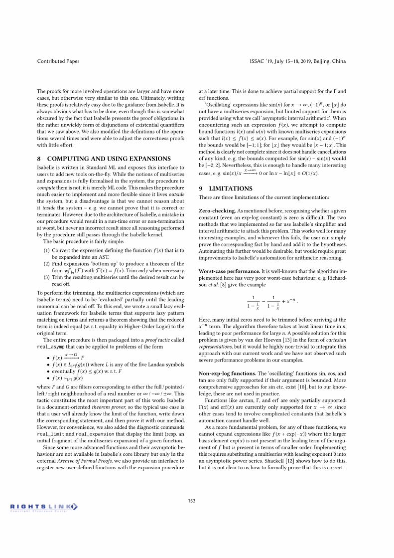
The proofs for more involved operations are larger and have morecases, but otherwise very similar to this one. Ultimately, writingthese proofs is relatively easy due to the guidance from Isabelle. It isalways obvious what has to be done, even though this is somewhatobscured by the fact that Isabelle presents the proof obligations inthe rather unwieldy form of disjunctions of existential quantifiersthat we saw above. We also modified the definitions of the opera-tions several times and were able to adjust the correctness proofswith little effort.
8 COMPUTING AND USING EXPANSIONSIsabelle is written in Standard ML and exposes this interface tousers to add new tools on-the-fly. While the notions of multiseriesand expansions is fully formalised in the system, the procedure tocompute them is not; it is merelyML code. This makes the proceduremuch easier to implement and more flexible since it lives outsidethe system, but a disadvantage is that we cannot reason aboutit inside the system – e. g. we cannot prove that it is correct orterminates. However, due to the architecture of Isabelle, a mistake inour procedure would result in a run-time error or non-terminationat worst, but never an incorrect result since all reasoning performedby the procedure still passes through the Isabelle kernel.
The basic procedure is fairly simple:(1) Convert the expression defining the function f (x) that is to
be expanded into an AST.(2) Find expansions ‘bottom up’ to produce a theorem of the
form wf bs(F ) with F (x) = f (x). Trim only when necessary.(3) Trim the resulting multiseries until the desired result can be
read off.To perform the trimming, the multiseries expressions (which areIsabelle terms) need to be ‘evaluated’ partially until the leadingmonomial can be read off. To this end, we wrote a small lazy eval-uation framework for Isabelle terms that supports lazy patternmatching on terms and returns a theorem showing that the reducedterm is indeed equal (w. r. t. equality in Higher-Order Logic) to theoriginal term.
The entire procedure is then packaged into a proof tactic calledreal_asymp that can be applied to problems of the form
• f (x) x→G−−−−−→ F• f (x) ∈ L[F ](д(x)) where L is any of the five Landau symbols• eventually f (x) ≤ д(x) w. r. t. F• f (x) ∼[F ] д(x)
where F andG are filters corresponding to either the full / pointed /left / right neighbourhood of a real number or ∞ /−∞ /±∞. Thistactic constitutes the most important part of this work: Isabelleis a document-oriented theorem prover, so the typical use case isthat a user will already know the limit of the function, write downthe corresponding statement, and then prove it with our method.However, for convenience, we also added the diagnostic commandsreal_limit and real_expansion that display the limit (resp. aninitial fragment of the multiseries expansion) of a given function.
Since some more advanced functions and their asymptotic be-haviour are not available in Isabelle’s core library but only in theexternal Archive of Formal Proofs, we also provide an interface toregister new user-defined functions with the expansion procedure
at a later time. This is done to achieve partial support for the Γ anderf functions.
‘Oscillating’ expressions like sin(x) for x →∞, (−1)n , or ⌊x⌋ donot have a multiseries expansion, but limited support for them isprovided using what we call ‘asymptotic interval arithmetic’: Whenencountering such an expression f (x), we attempt to computebound functions l(x) and u(x) with known multiseries expansionssuch that l(x) ≤ f (x) ≤ u(x). For example, for sin(x) and (−1)nthe bounds would be [−1; 1]; for ⌊x⌋ they would be [x − 1;x]. Thismethod is clearly not complete since it does not handle cancellationsof any kind; e. g. the bounds computed for sin(x) − sin(x) wouldbe [−2; 2]. Nevertheless, this is enough to handle many interestingcases, e. g. sin(x)/x x→∞−−−−−→ 0 or lnx − ln⌊x⌋ ∈ O(1/x).
9 LIMITATIONSThere are three limitations of the current implementation:
Zero-checking.Asmentioned before, recognising whether a givenconstant (even an exp-log constant) is zero is difficult. The twomethods that we implemented so far use Isabelle’s simplifier andinterval arithmetic to attack this problem. This works well for manyinteresting examples, and whenever this fails, the user can simplyprove the corresponding fact by hand and add it to the hypotheses.Automating this further would be desirable, but would require greatimprovements to Isabelle’s automation for arithmetic reasoning.
Worst-case performance. It is well-known that the algorithm im-plemented here has very poor worst-case behaviour; e. g. Richard-son et al. [8] give the example
11 − 1
x− 1
1 − 1x+ x−n .
Here, many initial zeros need to be trimmed before arriving at thex−n term. The algorithm therefore takes at least linear time in n,leading to poor performance for large n. A possible solution for thisproblem is given by van der Hoeven [13] in the form of cartesianrepresentations, but it would be highly non-trivial to integrate thisapproach with our current work and we have not observed suchsevere performance problems in our examples.
Non-exp-log functions. The ‘oscillating’ functions sin, cos, andtan are only fully supported if their argument is bounded. Morecomprehensive approaches for sin etc. exist [10], but to our know-ledge, these are not used in practice.
Functions like arctan, Γ, and erf are only partially supported:Γ(x) and erf(x) are currently only supported for x → ∞ sinceother cases tend to involve complicated constants that Isabelle’sautomation cannot handle well.
As a more fundamental problem, for any of these functions, wecannot expand expressions like f (x + exp(−x)) where the largerbasis element exp(x) is not present in the leading term of the argu-ment of f but is present in terms of smaller order. Implementingthis requires substituting a multiseries with leading exponent 0 intoan asymptotic power series. Shackell [12] shows how to do this,but it is not clear to us how to formally prove that this is correct.
7
Contributed Paper ISSAC ’19, July 15–18, 2019, Beijing, China
153

10 EVALUATIONWe evaluated our procedure on a large number of examples, in-cluding the list given in Section 8 of Gruntz’s PhD thesis [4]. Ac-cording to Gruntz, this list consists of various problems that weredifficult for computer algebra systems in the early 1990s. IndeedMaxima still returns an incorrect result for one of them.2 All ofthe 20 exp-log examples can be proven fully automatically by ourtactic within less than a second (average 0.24 s, maximum 0.65 s).Of the 17 non-exp-log examples, most lie outside the scope of ourprocedure due to unsupported functions (e. g. Bessel functions) orour incomplete support for Γ and erf . The 5 that are supported,however, all work in ≤ 2.5 s . Our list of examples can be found inthe file src/HOL/Real_Asymp/Real_Asymp_Examples.thy of theIsabelle distribution. A short user manual is also provided.
Let us return to our introductory example from Figure 1 andcompare our tactic with two CASs capable of handling additionalassumptions on the parameters, Mathematica and Maple.
Maple computes the limit to be 0 in 0.8 s. However, this alonedoes not tell us that the approach is from the right. If we force Mapleto really compute the leading term of the expansion by multiplyingthe function with ln1+ ε2 x and then asking for the limit, it gives upalmost immediately and returns the unevaluated expression.
Mathematica computes the limit to be 0 in 21 s. If we force itto compute the leading term, it produces the correct result in 463 s,but it also imposes the unnecessary side condition ε < 1.
Our tactic fails on this example with an errormessage indicatingthat it could not determine the sign of lnb · ε . The reason for thisis that the simplifier does not use the theorem x < 0 ∧ y > 0 =⇒x ·y < 0 by default. If we add this to the simplifier’s rewriting rules,the tactic successfully proves the limit to be 0+ in 0.3 s. It is evenable to compute the leading term − 1
2ε lnb · ln−1− ε2 x in 0.4 s.All in all, these examples show that, within its scope, our tactic
works well and perhaps even handles parameters somewhat bet-ter than proprietary CASs like Mathematica and Maple. In general,however, these CASs are of course much better both in terms of per-formance and number of supported functions. Still, we are pleasedwith this result, especially considering the immense additional dif-ficulty imposed by working inside a proof assistant where we wantnot only a result, but a proof.
11 RELATEDWORKThe first complete algorithm for the computation of exp-log func-tions was given by Shackell in 1990 [11]. Gruntz built on this al-gorithm and implemented it in Maple [4]. Gruntz’s algorithm waslater also implemented in Mathematica by Richter [9]. As stated be-fore, our work builds directly on themultiseries approach presentedby Richardson et al. [8].
In our prior work on the proof of the Akra–Bazzi theorem [3],we introduced some very simple automation related to asymptot-ics, e. g. to automatically prove or disprove statements of the formf (x) ∈ O(д(x)) where f and д are products of powers of iteratedlogarithms, e. g. x lnx ∈ O(x2(ln lnx)3). Apart from Isabelle/HOL,there are some other systems that have a library around limits
2Maxima claims that limx→∞ ln ln(x + exp(ln x ln ln x ))/ln ln ln(exp(x ) + x ) = 0,whereas the correct result is 1. We reported this bug in February 2018 but have notreceived a response.
and asymptotics (e. g. Coq, HOL Light, Mizar), but to our know-ledge, none of them has any automation for proving limits or otherasymptotic properties for any non-trivial class of problems.
12 CONCLUSIONWe provide the first implementation of automated real asymptoticsinside a proof assistant. The procedure provides:• full support for basic arithmetic, exp, ln, roots, and | · |• full support for sin, cos, and tan at finite points• ‘best effort’ support using interval arithmetic for oscillatingfunctions like sin, cos, tan at infinity and ⌊·⌋ and ⌈·⌉• partial support for arctan, Γ, and erf• support for parameters
All results produced by the procedure are trustworthy by construc-tion as they pass through the Isabelle kernel, which reduces themdown to definitions and basic logical inferences. On most practicalexamples, the procedure works quickly and fully automatically.
Acknowledgements.Wewould like to thank Joris van der Hoevenand Bruno Salvy for their help in understanding Multiseries andMaximilian P. L. Haslbeck and Kristina Magnussen for commentson a draft of this paper. We also thank Andrei Popescu for helpingus with coinduction, and the reviewers for their comments. Thiswork was supported by DFG grant NI 491/16-1.
REFERENCES[1] Julian Biendarra, Jasmin Christian Blanchette, Aymeric Bouzy, Martin Desharnais,
Mathias Fleury, Johannes Hölzl, Ondřej Kunčar, Andreas Lochbihler, FabianMeier,Lorenz Panny, Andrei Popescu, Christian Sternagel, René Thiemann, and DmitriyTraytel. 2017. Foundational (Co)datatypes and (Co)recursion for Higher-OrderLogic. In Frontiers of Combining Systems, Clare Dixon and Marcelo Finger (Eds.).Springer International Publishing, Cham, 3–21.
[2] Nicolas Bourbaki. 1971. Topologie générale.[3] Manuel Eberl. 2017. Proving Divide and Conquer Complexities in Isabelle/
HOL. Journal of Automated Reasoning 58, 4 (01 Apr 2017), 483–508. https://doi.org/10.1007/s10817-016-9378-0
[4] Dominik Gruntz. 1996. On Computing Limits in a Symbolic Manipulation System.Ph.D. Dissertation. ETH Zürich.
[5] Johannes Hölzl. 2009. Proving Inequalities over Reals with Computation inIsabelle/HOL. In Proceedings of the ACM SIGSAM 2009 International Workshopon Programming Languages for Mechanized Mathematics Systems (PLMMS’09),Gabriel Dos Reis and Laurent Théry (Eds.). Munich, 38–45.
[6] Johannes Hölzl, Fabian Immler, and Brian Huffman. 2013. Type Classes andFilters for Mathematical Analysis in Isabelle/HOL. In Proceedings of the 4thInternational Conference on Interactive Theorem Proving (ITP’13). Springer-Verlag,Berlin, Heidelberg, 279–294. https://doi.org/10.1007/978-3-642-39634-2_21
[7] Daniel Richardson. 1995. A Simplified Method of Recognizing Zero AmongElementary Constants. In Proceedings of the 1995 International Symposium onSymbolic and Algebraic Computation (ISSAC ’95). ACM, New York, NY, USA,104–109. https://doi.org/10.1145/220346.220360
[8] Daniel Richardson, Bruno Salvy, John Shackell, and Joris Van der Hoeven. 1996.Asymptotic Expansions of exp-log Functions. In Proceedings of the 1996 Interna-tional Symposium on Symbolic and Algebraic Computation (ISSAC ’96). ACM, NewYork, NY, USA, 309–313. https://doi.org/10.1145/236869.237089
[9] Udo Richter. 2005. Automatische Berechnung von Grenzwerten und Implementier-ung in Mathematica. diploma thesis. Universität Kassel.
[10] Bruno Salvy and John Shackell. 2010. Measured limits and multiseries. Journal ofthe London Mathematical Society 82, 3 (2010), 747–762. https://doi.org/10.1112/jlms/jdq057
[11] John Shackell. 1990. Growth estimates for exp–log functions. Journal of Sym-bolic Computation 10, 6 (1990), 611–632. https://doi.org/10.1016/S0747-7171(08)80161-7
[12] John R. Shackell. 2004. Symbolic Asymptotics. Algorithms and Computation inMathematics, Vol. 12. Springer Berlin–Heidelberg.
[13] Joris van der Hoeven. 1997. Automatic asymptotics. Ph.D. Dissertation. Écolepolytechnique, Palaiseau, France.
[14] Joris van der Hoeven. 2006. Transseries and real differential algebra. Lecture Notesin Mathematics, Vol. 1888. Springer-Verlag.
8
Contributed Paper ISSAC ’19, July 15–18, 2019, Beijing, China
154

B Divide-and-Conquer Recurrences
This chapter was originally published as an article in a peer-reviewed journal:
M. Eberl.Proving Divide and Conquer Complexities in Isabelle/HOL.Journal of Automated Reasoning, 58(4):483–508, Apr 2017, Springer Netherlands. © 2016DOI: 10.1007/s10817-016-9378-0.
I am the sole author of this article, thus all contributions are mine.
Synopsis: This work gives the rst formal proof of the Akra–Bazzi Theorem, a ‘cooking book’method to determine the asymptotic growth of solutions to the divide-and-conquer recur-rences that are often encountered in the analysis of divide-and-conquer algorithms. As asimple corollary of this, a generalised version of the well-known Master Theorem for divide-and-conquer recurrences is also obtained, including a proof method to facilitate applying itto concrete examples with minimal manual work. The usability of this is demonstrated onseveral textbook examples such as merge sort and Karatsuba multiplication.
On the following pages, the full article is reprinted by permission from Springer NatureCustomer Service Centre GmbH. The ocial version on SpringerLink can be found under theDOI cited above.
71
J Autom Reasoning (2017) 58:483–508DOI 10.1007/s10817-016-9378-0
Proving Divide and Conquer Complexities inIsabelle/HOL
Manuel Eberl1
Received: 23 July 2015 / Accepted: 3 June 2016 / Published online: 13 June 2016© Springer Science+Business Media Dordrecht 2016
Abstract The Akra–Bazzi method (Akra and Bazzi in Comput Optim Appl 10(2):195–210, 1998. doi:10.1023/A:1018373005182), a generalisation of the well-known MasterTheorem, is a useful tool for analysing the complexity of Divide and Conquer algo-rithms. This work describes a formalisation of the Akra–Bazzi method (as generalised byLeighton in Notes on better Master theorems for divide-and-conquer recurrences, 1996.http://courses.csail.mit.edu/6.046/spring04/handouts/akrabazzi.pdf) in the interactive theo-rem prover Isabelle/HOL and the derivation of a generalised version of the Master Theoremfrom it. We also provide some automated proof methods that facilitate the application of thisMaster Theorem and allow mostly automatic verification of Θ-bounds for these Divide andConquer recurrences. To our knowledge, this is the first formalisation of theorems for theanalysis of such recurrences.
Keywords Isabelle/HOL ·Master Theorem ·Akra–Bazzi ·Divide and Conquer algorithms ·Recurrences · Complexity · Landau symbols
1 Introduction
The Master Theorem is the textbook method taught in undergraduate algorithms lecturesfor analysing the asymptotic run-time complexity of many Divide and Conquer algorithms.The general form of the admissible algorithms is several non-recursive base cases and onerecursive case, in which a problem of size n is reduced to a fixed number a of subproblems ofsize n/b, which are then solved recursively and their solutions combined to a solution for theoriginal problem. One simple example is Merge Sort: lists of length ≤1 are always triviallysorted and thus returned unchanged (the base cases); lists of size ≥2 are split into half, each
This work was supported by DFG RTG 1480 (PUMA).
B Manuel [email protected]
1 Fakultät für Informatik, Technische Universität München, Garching, Germany
123

484 M. Eberl
half is sorted recursively, and the two sorted halves are then combined into a single sortedlist. The recurrence relation of this algorithm’s run-time function T is
T (n) = 2T( 12n
) + n
and the classical Master Theorem then states T ∈ Θ(n ln n). One problem with this is that,strictly speaking, the recurrence relation for T is actually something like
T (n) = T(⌊ 1
2n⌋) + T
(⌈ 12n
⌉) + n
since one certainly cannot split a list of length 3 into two lists of length 1.5. Intuitively, onemay think that the rounding does not change the asymptotic behaviour of the function, seeingas the rounding operations are asymptotically small disturbances. This is, in fact, the case,but proving it is not entirely trivial and is seldom done rigorously in textbooks or lectures,especially the case when both floors and ceilings are used at the same time, as in the exampleabove.1
In order to establish a basis for the verified run-time analysis of such algorithms, wewanted to formalise the Master Theorem in the theorem prover Isabelle/HOL. This must,of course, include rigorous handling of rounding operations. We therefore chose not to baseour formal proof on any of the literature proofs for the Master Theorem, but to instead provea generalisation known as the Akra–Bazzi method [1], and derive the Master Theorem as acorollary. As a pleasant side effect, this version of the Master Theorem supports much morecomplex recursion patterns than the classical Master Theorem from the literature.
To make the application of the Master Theorem in the theorem prover almost as simpleas on paper, we provided some proof automation machinery that facilitates the definition offunctions from Akra–Bazzi-type Divide and Conquer recurrences and allows applying theMaster Theorem to them in a mostly automatic way.
To provide some motivation, consider the following two recurrences, which are related toa deterministic selection algorithm and so-called Ham-Sandwich trees. They are far outsidethe scope of the classical Master Theorem, but their complexities can easily be found andformally proven in Isabelle/HOL with the generalised Master Theorem we formalised:
f1(n) = f1(⌊ n
5
⌋) + f1(⌊ 7n
10
⌋ + 6) + 12n
5 Result: f1 ∈ Θ(n)
f2(n) = f2(⌊ n
2
⌋) + f2(⌊ n
4
⌋) + 1 Result: f2 ∈ Θ(nlog2 ϕ) where ϕ = 1+√5
2
Outline In Sect. 2, we will list some related work on the type of recurrences that we focuson in this work. Section 3 then gives some important background information, namely aboutthe notation used in this work and the notions of integration and Landau symbols that areused in the formal proof.
Section 4 contains a formal description of the types of recurrences for which our results—the Akra–Bazzi theorem and the generalisedMaster Theorem—hold, and Sects. 5 and 6 statethese results. The formal Isabelle/HOL proof of the results is explained in Sect. 7. Section 8gives a list of the proof automation we developed for the Master Theorem as well as a fewexamples of its application.
Finally, Sect. 9 compares the scope of our version of theAkra–Bazzi theorem toLeighton’sand our Master Theorem to the ‘textbook’ version of the Master Theorem.
1 In Introduction to Algorithms [7], for example, only the ‘floor’ case is proven and the ‘ceiling’ case is statedto be analogous. The question of what happens when both floors and ceilings are used is not addressed.
123
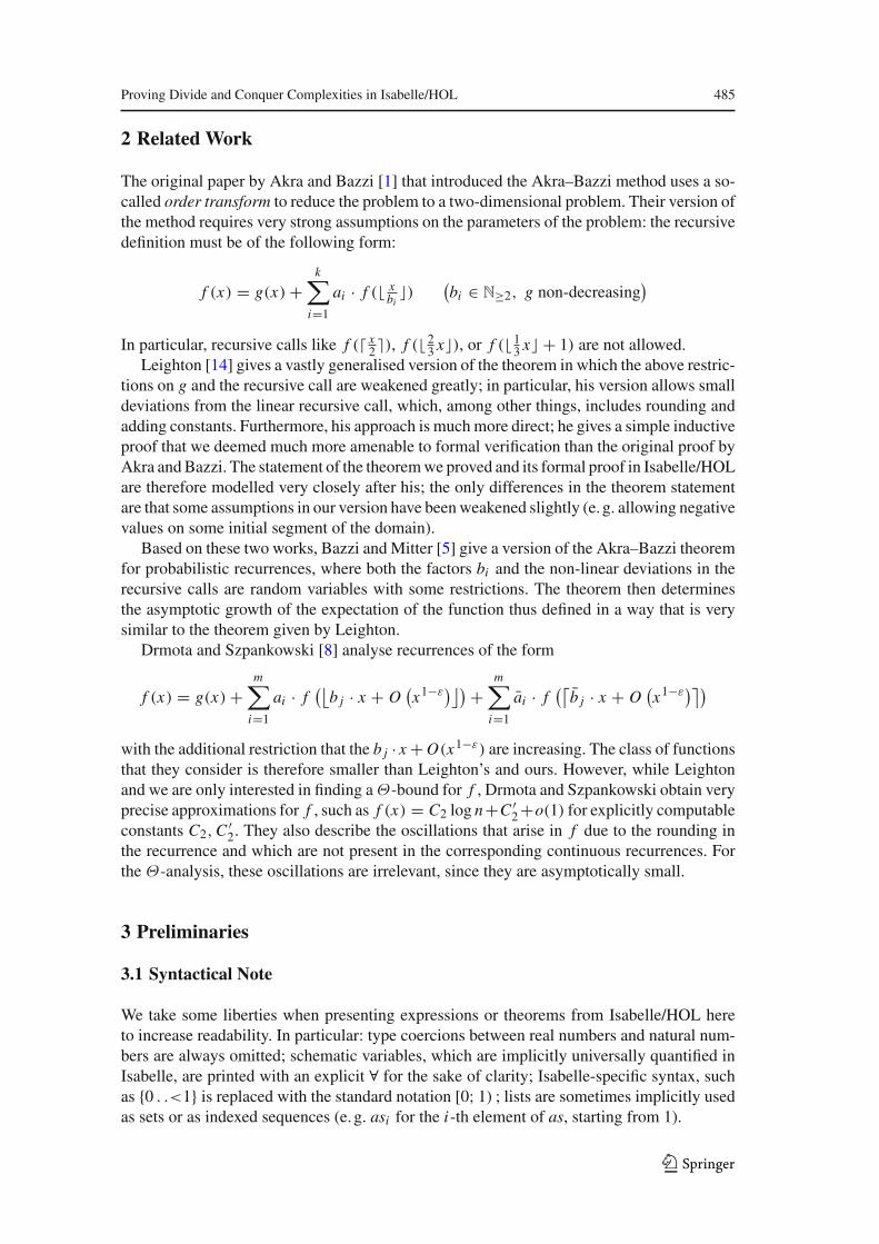
Proving Divide and Conquer Complexities in Isabelle/HOL 485
2 Related Work
The original paper by Akra and Bazzi [1] that introduced the Akra–Bazzi method uses a so-called order transform to reduce the problem to a two-dimensional problem. Their version ofthe method requires very strong assumptions on the parameters of the problem: the recursivedefinition must be of the following form:
f (x) = g(x) +k∑
i=1
ai · f ( xbi
) (bi ∈ N≥2, g non-decreasing
)
In particular, recursive calls like f ( x2 ), f ( 2
3 x), or f ( 13 x + 1) are not allowed.
Leighton [14] gives a vastly generalised version of the theorem in which the above restric-tions on g and the recursive call are weakened greatly; in particular, his version allows smalldeviations from the linear recursive call, which, among other things, includes rounding andadding constants. Furthermore, his approach is muchmore direct; he gives a simple inductiveproof that we deemed much more amenable to formal verification than the original proof byAkra andBazzi. The statement of the theoremwe proved and its formal proof in Isabelle/HOLare therefore modelled very closely after his; the only differences in the theorem statementare that some assumptions in our version have beenweakened slightly (e. g. allowing negativevalues on some initial segment of the domain).
Based on these two works, Bazzi and Mitter [5] give a version of the Akra–Bazzi theoremfor probabilistic recurrences, where both the factors bi and the non-linear deviations in therecursive calls are random variables with some restrictions. The theorem then determinesthe asymptotic growth of the expectation of the function thus defined in a way that is verysimilar to the theorem given by Leighton.
Drmota and Szpankowski [8] analyse recurrences of the form
f (x) = g(x) +m∑
i=1
ai · f(⌊
b j · x + O(x1−ε
)⌋) +m∑
i=1
ai · f(⌈
b j · x + O(x1−ε
)⌉)
with the additional restriction that the b j · x + O(x1−ε) are increasing. The class of functionsthat they consider is therefore smaller than Leighton’s and ours. However, while Leightonand we are only interested in finding aΘ-bound for f , Drmota and Szpankowski obtain veryprecise approximations for f , such as f (x) = C2 log n+C ′
2+o(1) for explicitly computableconstants C2, C ′
2. They also describe the oscillations that arise in f due to the rounding inthe recurrence and which are not present in the corresponding continuous recurrences. Forthe Θ-analysis, these oscillations are irrelevant, since they are asymptotically small.
3 Preliminaries
3.1 Syntactical Note
We take some liberties when presenting expressions or theorems from Isabelle/HOL hereto increase readability. In particular: type coercions between real numbers and natural num-bers are always omitted; schematic variables, which are implicitly universally quantified inIsabelle, are printed with an explicit ∀ for the sake of clarity; Isabelle-specific syntax, suchas 0 . .<1 is replaced with the standard notation [0; 1) ; lists are sometimes implicitly usedas sets or as indexed sequences (e. g. asi for the i-th element of as, starting from 1).
123

486 M. Eberl
Table 1 Definitions of the fiveLandau symbols f ∈ O(g) ←→ ∃c > 0. ∃x0. ∀x ≥ x0. | f (x)| ≤ c · |g(x)|
f ∈ o(g) ←→ ∀c > 0. ∃x0. ∀x ≥ x0. | f (x)| ≤ c · |g(x)|f ∈ (g) ←→ ∃c > 0. ∃x0. ∀x ≥ x0. | f (x)| ≥ c · |g(x)|f ∈ ω(g) ←→ ∀c > 0. ∃x0. ∀x ≥ x0. | f (x)| ≥ c · |g(x)|f ∈ Θ(g) ←→ f ∈ O(g) ∧ f ∈ (g)
A function taking some value x and returning some t that may depend on x will be writtenas λx . t , following Lambda calculus syntax as opposed to the traditional mathematical syntaxx → t . We will occasionally omit the ‘λ’ when it is clear from the context that we mean afunction and what the function variable is, particularly in Landau symbols (e. g. x ∈ O(x2)instead of (λx . x) ∈ O(λx . x2)).
3.2 Landau Symbols
3.2.1 Definition
Before stating the Akra–Bazzi theorem, we shall give the precise definition of the Landausymbols that were used in the Isabelle formalisation [10]. Since there was no suitable for-malisation of asymptotic growth in Isabelle/HOL, we created a library of Landau symbolsspecifically for the formalisation of the Akra–Bazzi method, but with other use cases in mindas well. The definitions we chose differ slightly from those given in Introduction to Algo-rithms by Cormen et al. [7]: for f ∈ O(g) to hold, they require f and g to be positive forsufficiently large inputs, whereas we do not. According to our definitions,
f ∈ O(g) ←→ − f ∈ O(g) ←→ f ∈ O(−g) ←→ − f ∈ O(−g).
This choice was made because, in our experience, formal reasoning with Landau symbols—especially automatic reasoning—becomes easier this way.
Table 1 shows the definitions of our Landau symbols. In Isabelle, Landau symbols aredefined for functions from any (not necessarily linearly) ordered set to any linearly-orderedfield. The restriction to fields was made due to the fact that the existence of multiplicativeinverses makes Landau symbols more ‘well-behaved’, and one may even argue that Landausymbols for functions into e. g. the natural numbers do not make much sense—one willprobably always want to view such functions as functions into the reals.
There is one prior formalisation of Landau symbols in Isabelle by Avigad et al. [2]. It isrelated to their proof of the Prime Number theorem. They only defined the symbol ‘O’, andthey did so in the following fashion:
O( f ) = h | ∃c. ∀x . |h(x)| ≤ c · | f (x)|
This definition differs from the commonly used one in so far as this one requires the inequalityto hold on all inputs, not just for sufficiently large inputs. If the inputs are natural numbers, thetwo are almost equivalent, but in the context of the Akra–Bazzi theorem, we also use Landausymbols for functions of type R → R and then these two definitions are quite different. Wetherefore deemed it necessary to create our own library of Landau symbols.
123

Proving Divide and Conquer Complexities in Isabelle/HOL 487
3.2.2 Decision Procedure
During the process of proving the generalised Master Theorem, and particularly in its appli-cations, we encountered a great number of proof obligations like x ∈ O(x3), x2 ∈ o(x2 ln x),ln x ∈ ω(ln ln x), etc. These problems all have the following in common:
– They are of the form f ∈ L(g), where L is a Landau symbol and f, g : R → R areproducts of ‘elementary buildingblocks’ like the identity function and iterated logarithms.
– The building blocks can be ordered linearly w. r. t. their growth (e.g. x , ln x , ln ln x ,…)in such a way that the growth rate of any positive power of a function in the sequenceeclipses that of any power of the subsequent one (e.g. x p ∈ ω((ln x)q) for any p, q ∈ R
with p > 0).– These problems are typically very tedious to prove formally.– Most mathematicians would dismiss them as trivial and not even bother proving them by
hand in a pen-and-paper proof.
The obvious course of action was therefore to develop automation machinery to dischargethese proof obligations automatically. In the following, we will sketch the decision procedurewe developed for this problem without going into too much detail.
Definition 1 (Families of functions) We call F ⊆ RR a family of functions if
– F is closed under multiplication and multiplicative inverse– each function in F is positive for all sufficiently large inputs– F is linearly ordered in the sense that for any f, f ∈ F , at least one of f ∈ o( f ),
f ∈ ω( f ), and f ∈ Θ( f ) holds
Examples for such families are λx . x p | p ∈ R or λx . ax | a ∈ R>0.Definition 2 (Dominating families) We say that a family F dominates a family G if
– there exists an f ∈ F such that g ∈ o( f ) for all g ∈ G– f (x) ∈ o( f (x)) implies f (x) · g(x) ∈ o( f (x) · g(x)) for any f, f ∈ F and g, g ∈ G
If F dominates G, we immediately have for all f, f ∈ F and g, g ∈ G:f (x) · g(x) ∈ o( f (x) · g(x)) ←→ f ∈ o( f ) ∨ ( f ∈ Θ( f ) ∧ g ∈ o(g))
f (x) · g(x) ∈ O( f (x) · g(x)) ←→ f ∈ o( f ) ∨ ( f ∈ Θ( f ) ∧ g ∈ O(g))
f (x) · g(x) ∈ Θ( f (x) · g(x)) ←→ f ∈ Θ( f ) ∧ g ∈ Θ(g)
In other words: o, O , and Θ on F · G behave analogously to <, ≤, and = on pairs withlexicographic ordering.
Furthermore, it is obvious that if F dominates G and G dominates H, then F dominatesG ·H. This notion of transitivity implies that we can lift the above result on pairs to sequenceswhere each family dominates the next. We can thus reduce any statement of the form
f1(x) . . . fn(x) ∈ L( f1(x) . . . fn(x)) (with L ∈ o, O,Θ and fi , fi ∈ Fi )
to a statement involving only Boolean connectives and expressions of the form fi ∈ l( fi )
for l ∈ o, O,Θ.Of course, this means that if the Fi are chosen such that we can decide fi ∈ l( fi ), we
can also decide f ∈ L( f ). In our decision procedure, the admissible function families arepowers of iterated logarithms; i. e. for each fixed k ∈ N, the functions of the form
λx . (ln . . . ln︸ ︷︷ ︸k times
x)p (for some p ∈ R)
123

488 M. Eberl
form one family. Deciding fk ∈ l( fk) for two functions in such a family can then be doneeasily by comparing the exponents.
Our decision procedure therefore simply analyses a goal like x ∈ o(x ln x) and rewrites itto x1(ln x)0 ∈ o(x1(ln x)1). By the above result, this holds iff 1 < 1∨(1 = 1∧0 < 1), whichIsabelle’s simplifier can easily prove automatically. We integrated this decision procedureinto Isabelle’s simplifier, so proof obligations of this form will automatically be rewritten tonecessary and sufficient conditions containing only Boolean connectives and comparisonson the exponents. Additionally, if these exponents are numeric constants, the conditions arethen proven (or disproven) automatically by the simplifier. This made many of our proofsand the application of our main results much easier.
In addition to this decision procedure, we also have simplifier setup that can:
– Simplify terms like L( f + g) to L(g) if f ∈ o(g) or to L( f ) if g ∈ o( f )
– Cancel common factors like h from f · h ∈ L(g · h) if h(x) is non-zero for large enoughx
– Perform simplifications on functions under a Landau symbol that are valid for sufficientlylarge values, e. g. ln(2x) = ln 2 + ln x . (This is not valid in Isabelle/HOL for x ≤ 0)
We initially formalised the proof of the asymptotic inequalities described in Sect. 7.2 inan elementary way. The resulting proofs were complex and virtually unreadable. After theintroduction of Landau symbols and with heavy use of the automation we just described, wewere able to more than halve the length of these proofs and make them significantly morereadable.
3.3 Integration
Since the statement of the Akra–Bazzi theorem contains an integral, we need to decide on adefinition of integration and a formalisation thereof. Isabelle contains a number of differentintegrals, most notably the Henstock–Kurzweil integral (also known as the Gauge integral)on functions fromEuclidean spaces to normed real vector spaces and theBochner integral (anextension of the Lebesgue integral) on functions from ameasure space to the real numbers [3].
In the proof of the Akra–Bazzi theorem, we noticed that the only properties of integrationthat we actually needed are the following:
Integral of constant functions If a ≤ b and c ∈ R≥0, the constant function λx . c is integrableon [a; b] and
∫ b
ac dx = (b − a) · c.
Monotonicity If f and g are integrable on [a; b] and f (x) ≤ g(x) for all x ∈ [a; b], then∫ b
af (x) dx ≤
∫ b
ag(x) dx .
Integrability on sub-intervals If f is integrable on [a; d] and a ≤ b ≤ c ≤ d , then f is alsointegrable on [b; c] .
Splitting if f is integrable on [a; c] and a ≤ b ≤ c, then∫ b
af (x) dx +
∫ c
bf (x) dx =
∫ c
af (x) dx .
123

Proving Divide and Conquer Complexities in Isabelle/HOL 489
We therefore proved the Akra–Bazzi theorem generically w. r. t. the integral definition: thetheorem can be instantiated with any concept of integration and integrability that fulfils theabove four properties. We call such an integral admissible.
The ‘standard’ integrals like the Riemann, Lebesgue, Bochner, and Henstock–Kurzweilintegrals all fulfil these properties and are therefore admissible, as is the non-negativeLebesgue integral that ignores the negative part of the integrand. Notably, all of these aregeneralisations of the Riemann integral on non-negative functions. The natural question isthen: Are there any admissible ‘integrals’ that are not integrals in the usual sense, i. e. notmerely generalisations of the Riemann integral?
The answer to this is not immediately obvious, but it turns out that any admissible integralI must coincide with the Riemann integral on any function f that is both piecewise con-tinuous and I-integrable, but it can differ from the Riemann integral and its generalisationson non-piecewise-continuous functions. Since non-piecewise-continuous functions shouldrarely arise in the context of the Akra–Bazzi theorem, we shall not explore the issue furtherhere; a more detailed explanation and a proof can be found in the “Appendix”.
4 General Setting
Let us now set up the context in which the remainder of this work will be set: For our versionof the Akra–Bazzi method, we shall consider a recursively-defined function f : N → R
with the following properties:
f (x) ≥ 0 for all x ∈ [x0; x1)
f (x) = g(x) +k∑
i=1
ai · f (bi · x + hi (x)) for all x ≥ x1
for a natural number k ∈ N \ 0, a function g : N → R, natural numbers x0, x1 ∈ N, realcoefficients ai ∈ R, bi ∈ R, functions hi : N → R such that:
– g(x) ≥ 0 for all x ≥ x1– ai ≥ 0 for all i ∈ [1; k] and ai > 0 for at least one i ∈ [1; k]– bi ∈ (0; 1) for all i ∈ [1; k]– for every i ∈ [1; k], there exists an ε > 0 such that hi ∈ O(x/ ln1+ε x)
– bi x + hi (x) ∈ N and x0 ≤ bi · x + hi (x) < x for all i ∈ [1; k] and all x ≥ x1(well-definedness of f )
We will now explain the meaning of these variables.
The recursion structure The parameters x0, x1, k, ai , bi , and hi characterise the recursionstructure of the function f . To understand the role of the different parameters, it is useful tolook at them in the case when f describes the cost of a Divide & Conquer algorithm: thevalues between x0 and x1 are the costs of the base cases; the cost of the recursive case isdefined recursively as the sum of the costs of the recursive calls and the costs of combiningthe results of the calls. Each triple (ai , bi , hi ) corresponds to ai recursive calls of the formbi · x + hi (x) ; the costs of combining the results are represented by the function g.
Variation terms The hi represent asymptotically small variation terms in the recursive call,allowing some deviation from the linear term bi · x . This is not merely a nice gimmick—it is actually necessary to have something like this, since, due to the discreteness of the
123

490 M. Eberl
natural numbers, a purely linear term in the recursive call is impossible. This approach coversrounding and other deviations in a uniform way, as opposed to making ad-hoc argumentswhy certain kinds of rounding do not change the result.
For example, the terms f ( x2 ), f ( x
2 ), and f ( x2 + 42) would be admissible, as they
can be expressed as f (b · x + h(x)) for some b ∈ (0; 1) and some h : N → R whereh ∈ O(1). However, much larger deviations, such as f ( 1
2n − √n) , are also allowed.
Of course, enough base cases must be provided (i. e. x0 and x1 must be chosen largeenough and far enough apart) to fulfil the well-definedness conditions; a function ‘definition’like f (x) = f ( 3
4 x)+1 for x1 = 3 cannot be allowed since f (3) = f ( 94)+1 = f (3)+1
is contradictory.Leighton [14] mentions that the condition that the hi be in O(x/ ln1+ε x) for some ε > 0
is tight in some sense, since the recurrence f (x) = 2 f (x/2 + x/ ln x) has the asymptoticgrowth x lnΘ(1) x , whereas the recurrence f (x) = 2 f (x/2) (i. e. without the variation term)has the growth Θ(x).
5 The Akra–Bazzi Method
Having established the necessary context, we will now present the main theorems of theAkra–Bazzi method for the function f . To do this, we first need to define the characteristicnumber of an Akra–Bazzi recurrence: The contribution of the recursion structure (withoutthe ‘recombination costs’ g) to the asymptotic growth can be summarised as a single realnumber, which we call p. This number is defined implicitly as
k∑
i=1
ai · b pi = 1
If the ai are not all zero (which we assumed), this equation defines p uniquely. To show this,we consider the function
t : R → R>0, x →k∑
i=1
ai · b xi .
This function is continuous and t (x)–∞−−→ ∞ and t (x)
∞−−→ 0. Therefore, by the intermediatevalue theorem, some p such that
∑ki=1 ai · bp
i = 1 always exists, and since t is also strictlydecreasing, this p is unique.
We can now state the three variants of the Akra–Bazzi theorem, which give , O , and Θ
bounds on the growth of f :
Theorem 1 (Akra–Bazzi theorem, version) Fix g : R → R with g ∈ (g), i. e. g is anasymptotic lower bound for g. Assume that:
– f (x) > 0 for all sufficiently large x– g(x) ≥ 0 for all sufficiently large x– there exist real constants c > 0 and C with ∀i ∈ [1; k]. C < bi such that for all
sufficiently large x: ∀u ∈ [C · x; x]. g(u) ≤ cg(x)
– g is bounded above on every real interval [a; b] with a ≥ a0 for some a0– g(x)/x p+1 is integrable on any interval [a; b] with a ≥ a0 for some a0
Then
f ∈
(x p
(1 +
∫ x
t
g(u)
u p+1 du
))
for any sufficiently large t.
123
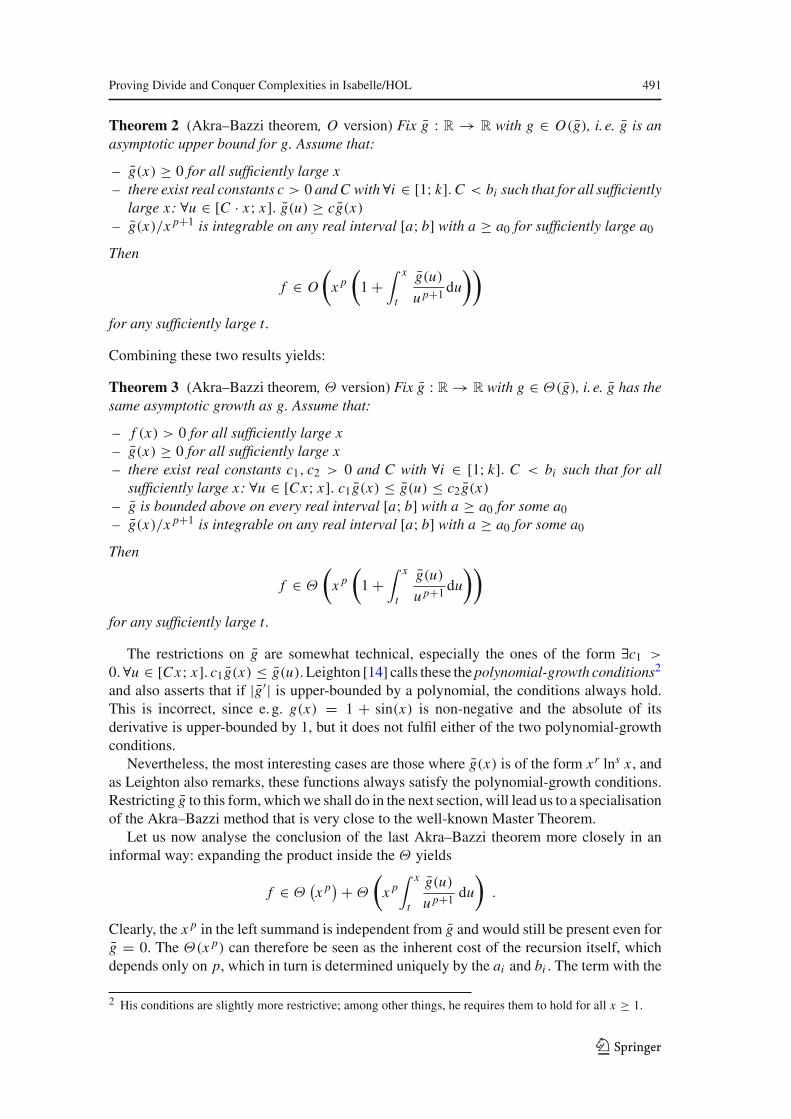
Proving Divide and Conquer Complexities in Isabelle/HOL 491
Theorem 2 (Akra–Bazzi theorem, O version) Fix g : R → R with g ∈ O(g), i. e. g is anasymptotic upper bound for g. Assume that:
– g(x) ≥ 0 for all sufficiently large x– there exist real constants c > 0 and C with ∀i ∈ [1; k]. C < bi such that for all sufficiently
large x: ∀u ∈ [C · x; x]. g(u) ≥ cg(x)
– g(x)/x p+1 is integrable on any real interval [a; b] with a ≥ a0 for sufficiently large a0
Then
f ∈ O
(x p
(1 +
∫ x
t
g(u)
u p+1 du
))
for any sufficiently large t.
Combining these two results yields:
Theorem 3 (Akra–Bazzi theorem, Θ version) Fix g : R → R with g ∈ Θ(g), i. e. g has thesame asymptotic growth as g. Assume that:
– f (x) > 0 for all sufficiently large x– g(x) ≥ 0 for all sufficiently large x– there exist real constants c1, c2 > 0 and C with ∀i ∈ [1; k]. C < bi such that for all
sufficiently large x: ∀u ∈ [Cx; x]. c1g(x) ≤ g(u) ≤ c2 g(x)
– g is bounded above on every real interval [a; b] with a ≥ a0 for some a0– g(x)/x p+1 is integrable on any real interval [a; b] with a ≥ a0 for some a0
Then
f ∈ Θ
(x p
(1 +
∫ x
t
g(u)
u p+1 du
))
for any sufficiently large t.
The restrictions on g are somewhat technical, especially the ones of the form ∃c1 >
0.∀u ∈ [Cx; x]. c1 g(x) ≤ g(u). Leighton [14] calls these thepolynomial-growth conditions2
and also asserts that if |g′| is upper-bounded by a polynomial, the conditions always hold.This is incorrect, since e. g. g(x) = 1 + sin(x) is non-negative and the absolute of itsderivative is upper-bounded by 1, but it does not fulfil either of the two polynomial-growthconditions.
Nevertheless, the most interesting cases are those where g(x) is of the form xr lns x , andas Leighton also remarks, these functions always satisfy the polynomial-growth conditions.Restricting g to this form, whichwe shall do in the next section, will lead us to a specialisationof the Akra–Bazzi method that is very close to the well-known Master Theorem.
Let us now analyse the conclusion of the last Akra–Bazzi theorem more closely in aninformal way: expanding the product inside the Θ yields
f ∈ Θ(x p) + Θ
(x p
∫ x
t
g(u)
u p+1 du
).
Clearly, the x p in the left summand is independent from g and would still be present even forg = 0. The Θ(x p) can therefore be seen as the inherent cost of the recursion itself, whichdepends only on p, which in turn is determined uniquely by the ai and bi . The term with the
2 His conditions are slightly more restrictive; among other things, he requires them to hold for all x ≥ 1.
123

492 M. Eberl
integral on the right, on the other hand, also depends on the recombination costs g(x), and itis big whenever g(x) is big.
It is also clear that the values of the base cases are completely irrelevant (as long as theyare non-negative).
6 The Master Theorem
If we look at a restricted class of functions g, we can make the last two observations of theprevious section a bit more precise: If g(x) is of the form xq for some q ∈ R, the conditionson g (non-negativity, polynomial growth, boundedness, integrability) are all satisfied. If theother conditions for the Akra–Bazzi theorem are satisfied, we have:
f ∈ Θ(x p) + Θ
(x p
∫ x
tuq−p−1du
)=
⎧⎨
⎩
Θ(x p) + Θ
(xq) = Θ
(x p) for q < p
Θ(x p) + Θ
(x p ln x
) = Θ(x p ln x
)for q = p
Θ(x p) + Θ
(xq) = Θ
(xq) for q > p
The three cases differ in how high the inherent costs of the recursion are compared to therecombination costs. In the first case, the recombination costs are smaller than the recursioncosts, which means that most of the work is done at the bottom of the recursion tree, sincethere are many leaves, but recombining them is cheap (‘bottom-heavy recursion’). In thethird case, the recombination costs dominate and most of the work will be done recombiningthe results near the top of the recursion tree (‘top-heavy recursion’). In the second case,the recursion costs and the recombination costs have a similar rate of growth (‘balancedrecursion’). This case can be generalised further by considering g(x) = x p lnq x .
This leads to our generalised Master Theorem:
Corollary 1 (Master Theorem)
Bottom-heavy recursion. If g ∈ O(xq) for some q < p, then f ∈ O(x p). If, additionally,f (x) is positive for all sufficiently large x, we even have f ∈Θ(x p).3
Balanced recursion.If g ∈ Θ(x p lnq x) for some q, then
f ∈
⎧⎪⎨
⎪⎩
Θ(x p) if q < −1
Θ(x p ln ln x) if q = −1
Θ(x p lnq+1 x) if q > −1
Top-heavy recursion. If g ∈ Θ(xq) for some q > p, then f ∈ Θ(xq) = Θ(g).
7 Proving the Akra–Bazzi Theorem and the Master Theorem
We shall now describe the proof of our version of the Akra–Bazzi theorem. Some parts ofthe proof are very technical; in these parts of the proof, we shall attempt to provide thereader with a good high-level understanding of what must be proven and how we proved itwithout mentioning toomany details. For more details, we refer the reader to the formal proof
3 Note that due to the other constraints on f and g, the condition that f (x) is positive for all sufficiently largex must hold if either g(x) is positive for all sufficiently large x or f (x) is positive in all the base cases, i. e.for x ∈ [x0; x1).
123

Proving Divide and Conquer Complexities in Isabelle/HOL 493
Fig. 1 The locale akra_bazzi_function that formally captures the conditions imposed upon the recursively-defined function f
development in the Archive of Formal Proofs [9] or, where applicable, Leighton’s proof [14].In any case, we recommend that readers familiarise themselves with Leighton’s proof beforeattempting to understand ours.
7.1 Formal Setting
First of all, we will explain how the conditions mentioned in Sect. 4 are stated formally inIsabelle/HOL: We use a locale [4] called akra_bazzi_function. A locale is a named contextthat contains fixed variables, assumptions, and definitions. Such a locale can be instantiatedby providing values for the fixed variables and proving that its assumptions hold for thesevalues. Instantiating a locale gives the user access to all the facts thatwere proven in this locale,specialised to the specific values that it was instantiated with. Figure 1 shows the definitionof the locale akra_bazzi_function, modulo some insignificant notational adjustments.
The only difference to the conditions stated in Sect. 4 is that the recursive calls are of theshape f (tsi (x)) instead of f (bi · x +hi x). The reason for this is that the latter would requireexpressing a call like f ( 1
2 x) in the rather awkward form f ( 12 x + ( 12 x − 1
2 x)), whereasthe former is more direct.
The conditions on the recursive calls are replaced by the condition that all the tsi beAkra–Bazzi terms, where
definition akra_bazzi_term(x0, x1, b, t) =(∃ ε h. ε > 0 ∧ h ∈ O(λx . x/ ln1+ε x) ∧
(∀x ≥x1. t (x) ≥ x0 ∧ t (x) < x ∧ b · x + h(x) = t (x))) .
One can then easily prove introduction rules to discharge this condition for specific formsof recursive calls, e. g.
lemma akra_bazzi_term_ceiling:
assumes b > 0 and b < 1 and x0 ≤ b · x1 and (1 − b) · x1 ≥ 1
shows akra_bazzi_term(x0, x1, b, λx . b · x)
Provided that such rules exist for every recursive call occurring in the recursive equationof f , this condition and most of the other locale assumptions contain only the constants as,bs, k, x0, and x1 and can therefore be solved by simple evaluation for a concrete function fwith concrete values for as, bs, etc. The remaining conditions are:
123
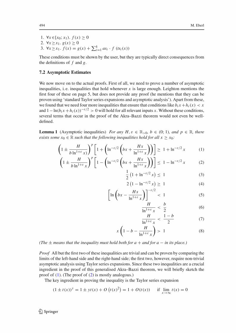
494 M. Eberl
1. ∀x ∈[x0; x1). f (x) ≥ 02. ∀x ≥x1. g(x) ≥ 03. ∀x ≥x1. f (x) = g(x) + ∑k
i=1 asi · f (tsi (x))
These conditions must be shown by the user, but they are typically direct consequences fromthe definitions of f and g.
7.2 Asymptotic Estimates
We now move on to the actual proofs. First of all, we need to prove a number of asymptoticinequalities, i. e. inequalities that hold whenever x is large enough. Leighton mentions thefirst four of these on page 5, but does not provide any proof (he mentions that they can beproven using ‘standard Taylor series expansions and asymptotic analysis’). Apart from these,we found that we need four more inequalities that ensure that conditions like bi x +hi (x) < xand 1− ln(bi x +hi (x))−ε/2 > 0 will hold for all relevant inputs x . Without these conditions,several terms that occur in the proof of the Akra–Bazzi theorem would not even be well-defined.
Lemma 1 (Asymptotic inequalities) For any H, ε ∈ R>0, b ∈ (0; 1), and p ∈ R, thereexists some x0 ∈ R such that the following inequalities hold for all x ≥ x0:
(1 ± H
b ln1+ε x)
)p [1 +
(ln−ε/2
(bx + H x
ln1+ε x
))]≥ 1 + ln−ε/2 x (1)
(1 ± H
b ln1+ε x
)p [1 −
(ln−ε/2
(bx + H x
ln1+ε x
))]≤ 1 − ln−ε/2 x (2)
1
2
(1 + ln−ε/2 x
) ≤ 1 (3)
2(1 − ln−ε/2 x
) ≥ 1 (4)[ln
(bx − H x
ln1+ε x
)]−ε/2
< 1 (5)
H
ln1+ε x<
b
2(6)
H
ln1+ε x<
1 − b
2(7)
x
(1 − b − H
ln1+ε x
)> 1 (8)
(The ± means that the inequality must hold both for a + and for a − in its place.)
Proof All but the first two of these inequalities are trivial and can be proven by comparing thelimits of the left-hand side and the right-hand side; the first two, however, require non-trivialasymptotic analysis using Taylor series expansions. Since these two inequalities are a crucialingredient in the proof of this generalised Akra–Bazzi theorem, we will briefly sketch theproof of (1). (The proof of (2) is mostly analogous.)
The key ingredient in proving the inequality is the Taylor series expansion
(1 ± t (x))y = 1 ± yt (x) + O(t (x)2
) = 1 + O(t (x)) if limx→∞ t (x) = 0
123

Proving Divide and Conquer Complexities in Isabelle/HOL 495
In the following, we will indicate such an expansion with the symbolTaylor= and a curly
bracket that denotes which term is taken to be t (x) in the expansion.First of all, we estimate the first factor on the left-hand side with4
(1 ±
t (x)︷ ︸︸ ︷H
b ln1+ε x
)pTaylor= 1 + O
(ln−1−ε x
) = 1 + o(ln−1−ε/2 x
)
Moreover, we have in the second factor:
ln−ε/2(
bx + H x
ln1+ε x
)
=[ln
(bx
(1 + H
b ln1+ε x
))]−ε/2
=[ln bx + ln
(1 + H
b ln1+ε x
)]−ε/2
= (ln−ε/2 bx
) [1 + 1
ln bxln
(1 + H
b ln1+ε x
)
︸ ︷︷ ︸t (x)
]−ε/2Taylor=
= (ln−ε/2 bx
) [1 + O
(1
ln bxln
(1 + H
b ln1+ε x
))]
= (ln−ε/2 bx
) + (ln−1−ε/2 bx
)O
(ln
(1 + H
b ln1+ε x
))
= (ln−ε/2 bx
) + (ln−1−ε/2 bx
)o(1)
= (ln−ε/2 bx
) + o(ln−1−ε/2 x
)
Combining these two asymptotic estimates, we have:
(1 ± H
b ln1+ε x
)p [1 +
(ln−ε/2
(bx + H x
ln1+ε x
))]
= [1 + o
(ln−1−ε/2 x
)] [1 + (
ln−ε/2 bx) + o
(ln−1−ε/2 x
)]
= 1 + (ln bx)−ε/2 + o(ln−1−ε/2 x
)
= 1 + (ln b + ln x)−ε/2 + o(ln−1−ε/2 x
)
= 1 + (ln−ε/2 x
)(1 + ln b
ln x︸︷︷︸t (x)
)−ε/2
+ o(ln−1−ε/2 x
) Taylor=
= 1 + (ln−ε/2 x
) (1 − ε ln b
2 ln x+ O
(ln−2 x
)) + o(ln−1−ε/2 x
)
= 1 + ln−ε/2 x +[−ε ln b
2ln−1−ε/2 x + o
(ln−1−ε/2 x
)]
4 The notation here becomes a bit informal. Terms like f (x)+ O(g(x)) stand for the set f (x)+h(x) | h(x) ∈O(g(x)) and all equality symbols are then essentially set inclusions, i. e. f (x) + O(. . .) = g(x) + O(. . .)
means that the left-hand side is a subset of the right-hand side.
123

496 M. Eberl
Since b∈(0; 1), we have ln b < 0. Therefore, the term in brackets will be positive forsufficiently large x and we have:
≥ 1 + ln−ε/2 x
7.3 The Continuous Akra–Bazzi Theorem
For the next part, we closely followLeighton’s proof (pp. 6–8). Herewe prove theAkra–Bazzitheorem for continuous recurrences, i. e. a function f : R → R that fulfils all the conditionsstated before, but not just on N, but on R. We therefore look at the following setting, whichis essentially the real-valued analogue to the setting described in Sect. 4:
Consider f : R → R with the following properties:
f (x) ≥ 0 for all x ∈ [x0; x1]
f (x) = g(x) +k∑
i=1
ai · f (bi · x + hi (x)) for all x > x1
for a natural number k ∈ N \ 0, a function g : R → R, natural numbers x0, x1 ∈ R, realcoefficients ai ∈ R, bi ∈ R, functions hi : N → R, and p ∈ R such that:
– g(x) ≥ 0 for all x ≥ x0– ai ≥ 0 for all i ∈ [1; k] and ai > 0 for at least one i ∈ [1; k]– bi ∈ (0; 1) for all i ∈ [1; k]– for every i ∈ [1; k], there exists an εi > 0 such that hi ∈ O(x/ ln1+εi x)
–∑k
i=1 ai · bpi = 1
– g(u)u−p−1 is integrable on [x0; x] for any x ≥ x0
We can assume w.l.o.g. that all the hi fulfil hi ∈ O(x/ ln1+ε x) for the same ε by choosingthe minimum of all the εi values. It is then clear that there exists a constant H such that, forsufficiently large x , we have |hi (x)| ≤ H x ln−1−ε x for all i ∈ [1; k].
We also assume that x0 and x1 are chosen large enough such that the following inequalitieshold:
– 1 ≤ x0 ≤ 12bi x1 for all i ∈ [1; k]
– |hi (x)| ≤ H x ln x−1−ε for all i ∈ [1; k] and all x ≥ x1– the inequalities (1) to (8) from Lemma 1 for any b ∈ b1 . . . bk and all x ≥ x0– there exists some real number C such that Cx ≤ bi x − H x ln−1−ε x for any i ∈ [1; k]
and all x ≥ x1
7.3.1 The Lower Bound
We will now show how to obtain an asymptotic lower bound on f (x). For this, we furtherhave to assume the existence of positive and finite bounds
F := infx∈[x0;x1]
f (x) and G:= supx∈[x0;x1]
g(x)
and the growth condition ∀x ≥ x1. ∀u ∈ [Cx; x]. c2g(x) ≥ g(u) for some c2 > 0. We canthen show the following two lemmas:
123

Proving Divide and Conquer Complexities in Isabelle/HOL 497
Lemma 2 There exists a c4 > 0 such that, for any i ∈ [1; k] and all x ≥ x1:
x p∫ x
bi x+hi (x)
g(u)
u p+1 du ≤ c4g(x)
Proof Technical and uninteresting; refer to Leighton’s Lemma 1 or our formal proof devel-opment for details.
Lemma 3 There exists a c5 > 0 with c5 ≤ 12c4
such that, for any x ∈ [x0; x1]:
2c5x p(1 +
∫ x
x0
g(u)
u p+1 du
)≤ f (x)
Proof We have x p ≤ max(x p0 , x p
1 ) and g(u)u−p−1 ≤ G ·max(x−p−10 , x−p−1
1 ); it is easy touse this to derive some bound c such that
2
Fx p
(1 +
∫ x
x0
g(u)
u p+1 du
)≤ c
and therefore
2
cx p
(1 +
∫ x
x0
g(u)
u p+1 du
)≤ F ≤ f (x).
Setting c5:=min(c−1, (2c4)−1) yields the desired bound. We can then show the following lower bound for f
Lemma 4
c5x p (1 + ln−ε/2 x) (
1 +∫ x
x0
g(u)
u p+1 du
)≤ f (x) for all x ≥ x0
Proof The proof is by induction over x with the base case x ∈ [x0; x1] and the inductivestep x > x1 while assuming that the induction hypothesis holds for all bi x + hi (x) for anyi ∈ [1; k]. This induction scheme is well-founded, since the bounds on the hi and inequality(8) imply bi x + hi (x) < x for any x ≥ x1, so the measure μ : R → N, x → xdecreases.
Base case We have x ∈ [x0; x1] and therefore:
c5x p (1 + ln−ε/2 x)
︸ ︷︷ ︸≤2
by Lemma 1.(3)
(1 +
∫ x
x0
g(u)
u p+1 du
)≤ 2c5x p
(1 +
∫ x
x0
g(u)
u p+1 du
)Lemma 3≤ f (x)
Induction step We have x > x1 and we assume the following induction hypothesis for anyi ∈ [1; k]:
c5(bi x + hi (x))p (1 + ln−ε/2(bi x + hi (x)))(
1 +∫ bi x+hi (x)
x0
g(u)
u p+1 du
)
(IH)
≤ f (bi x + hi (x))
We can then show:
c5x p (1 + ln−ε/2 x) (
1 +∫ x
x0
g(u)
u p+1 du
)Lemma 3≤
123

498 M. Eberl
≤ c5x p (1 + ln−ε/2 x) (
1 +∫ x
x0
g(u)
u p+1 du
)+ g(x) − 2c5c4g(x)
Lemma 1.(3)≤
≤ c5x p (1 + ln−ε/2 x) (
1 +∫ x
x0
g(u)
u p+1 du
)+ g(x) − c5c4
(1 + ln−ε/2 x
)g(x)
= g(x) + c5x p (1 + ln−ε/2 x)(1 +
∫ x
x0
g(u)
u p+1 du − c4x p
g(x)
)Lemma 2≤
= g(x) + c5x p (1 + ln−ε/2 x)(1 +
∫ x
x0
g(u)
u p+1 du −∫ x
bi x+hi (x)
g(u)
u p+1 du
)
= g(x) + c5x p (1 + ln−ε/2 x)(
1 +∫ bi x+hi (x)
x0
g(u)
u p+1 du
)
= g(x) +(
k∑
i=1
ai bpi
)
c5x p (1 + ln−ε/2 x)(
1 +∫ bi x+hi (x)
x0
g(u)
u p+1 du
)
= g(x) +k∑
i=1
ai c5bpi x p (1 + ln−ε/2 x
)(
1 +∫ bi x+hi (x)
x0
g(u)
u p+1 du
)
Let us now focus on the bpi x p
(1 + ln−ε/2 x
)term. Let s:=−1 if p ≥ 0 and s:=1 otherwise.
By applying first Lemma 1.(1) and then |hi (x)| ≤ H x ln x−1−ε , we have:
bpi x p (1 + ln−ε/2 x
) (1)≤ bpi x p
(1 + s H
bi ln1+ε x
)p (1 + ln−ε/2
(bi x + H x
ln1+ε x
))
=(
bi x + s H x
ln1+ε x
)p (1 + ln−ε/2
(bi x + H x
ln1+ε x
))
≤ (bi x + hi (x))p (1 + ln−ε/2 (bi x + h(x)))
Plugging this result into the inequality chain we interrupted before, we have:5
g(x) +k∑
i=1
ai c5bpi x p
(1 + ln−ε/2 x
)(
1 +∫ bi x+hi (x)
x0
g(u)
u p+1 du
)
≤ g(x) +k∑
i=1
ai c5 (bi x + hi (x))p[1 + ln−ε/2 (bi x + h(x))
](
1 +∫ bi x+hi (x)
x0
g(u)
u p+1 du
)(I H)≤
≤ g(x) +k∑
i=1
ai f (bi x + hi (x)) = f (x)
This concludes the induction. We have thus shown that for all x ≥ x0:
c5x p(1 +
∫ x
x0
g(u)
u p+1 du
)≤ c5x p (1 + ln−ε/2 x
)(1 +
∫ x
x0
g(u)
u p+1 du
)≤ f (x)
5 Note the implicit case distinction for p ≥ 0 and p < 0: for p ≥ 0, we need to show bi x − H x ln−1−ε x ≤bi x + hi (x) , whereas for p < 0 we need to show bi x + H x ln−1−ε x ≥ bi x + hi (x) since the negativeexponent flips the inequality. This case distinction is not mentioned by Leighton.
123

Proving Divide and Conquer Complexities in Isabelle/HOL 499
7.3.2 The Upper Bound
The proof of the upper bound is analogous with the following exceptions:
– The assumptions we need are supx∈[x0;x1] f (x) < ∞ and ∀x ≥ x1. ∀u ∈[Cx; x]. c1g(x) ≤ g(u) for some c1 > 0.
– The inequality we need to show by induction is
f (x) ≤ c6x p (1 − ln−ε/2 x) (
1 +∫ x
x0
g(u)
u p+1 du
)
7.4 Lifting to the Discrete Case
The remaining work in the proof of the Akra–Bazzi theorem is now to lift this result forcontinuous recurrences to discrete recurrences. We will again illustrate this for the lowerbound. We consider the setting given in Theorem 1.
First of all, we find values G > 0 and x0, x1 such that:
– x1 ≤ x0 ≤ x1– f (x) > 0 for all x ≥ x0– g(x) ≥ Gg(x) for all x ≥ x0 (possible because g ∈ (g))– g(x) ≥ 0 for all x ≥ x0– bi x + hi (x) ≥ x0 for all x ≥ x1 and i ∈ [1; k]Since g has the asymptotic lower bound g and we want to find an asymptotic lower bound
on f , it is natural that the function obtained by copying the definition of f , but with the costsg instead of g, should be an asymptotic lower bound on f . We therefore define the functionf : N → R as follows:
f (x) =max(0, f (x)/G) if x < x1g(x) + ∑k
i=1 ai f (bi x + hi (x)) otherwise
It is clear that f is non-negative everywhere, positive for large enough x , and G f (x) ≤ f (x)
for all x ≥ x0. Therefore, any asymptotic lower bound on f will also be a lower bound on f .Next, we find some x0 > x1 such that
– the asymptotic inequalities (1) to (8) hold for all x ≥ x0, c = H , b = bi for i ∈ [1; k]– |hi (x)| ≤ H x ln−1−ε x for all x ≥ x0 and i ∈ [1; k]– Cx ≤ bi x − H x ln−1−ε x for all x ≥ x0 and i ∈ [1; k]– g is bounded from above on all intervals that lie above x0– g(u) ≤ c2 g(x) for all x ≥ x0 and u ∈ [Cx; x]– f (x) > 0 and g(x) ≥ 0 for all x ≥ x0– g(u)u−p−1 is integrable on all intervals that lie above x0
and we find a x1 such that x1 ≥ 2bi
x0 for all i ∈ [1; k].We can then extend f to a function f : R → R using the following definition:
f (x) =
f (x) if x ≤ x1g(x) + ∑k
i=1 ai f (bi x + hi (x)) otherwise
Clearly, f (x) = f (x) for all natural numbers x .
123

500 M. Eberl
We apply the continuous lower bound theorem derived in the previous section to f (x)
with the ‘base cases’ between x0 and x1. This gives us the lower bound
c5x p(1 +
∫ x
x0
g(u)
u p+1 du
)≤ f (n)
For all natural numbers n ≥ x0, we then have:
Gc5n p(1 +
∫ n
x0
g(u)
u p+1 du
)≤ G f (n) = G f (n) ≤ f (n)
and therefore
f ∈
(n p
(1 +
∫ n
x0
g(u)
u p+1 du
)).
Since we could have chosen x0 larger as well if we had wanted to, we have essentially shownthat
f ∈
(n p
(1 +
∫ n
t
g(u)
u p+1 du
))
holds for any sufficiently large t .The formal proof of all of this consists mostly of finding large enough values for
x0 and x1 and proving that all required properties hold. For instance, the condition thatinf x∈[x0;x1] f (x) > 0 is fulfilled because, by definition, f (x) = f (x) only takes a finitenumber of values on the interval [x0; x1], all of which are positive.
This entire process of linking the assumptions of the discrete settings to the assumptionsof the continuous setting is very technical and intricate—it takes up almost a quarter of theentire proof of the Akra–Bazzi theorem—but mathematically uninteresting, which is whywe left out a lot of detail in this paper proof.
7.5 The Master Theorem
From the proof of the Akra–Bazzi theorem in the locale context akra_bazzi_function, wecan now show the Master Theorem, also inside this context. The proofs are straightforwardapplications of the Akra–Bazzi theorem. The user can then interpret the akra_bazzi_functionlocale for her function f and use the case of theMaster Theorem appropriate for her function.
In the Isabelle formalisation, the Master Theorem is split into five cases (cf. Table 2), withthe first case having a weak form (O) and a strong form (Θ).
Table 2 The five cases of the Master Theorem as formalised in Isabelle/HOL
Case name Assumptions Conclusion
Case 1 (O) g ∈ O(xq ) q < p f ∈ O(x p)
Case 1 g ∈ O(xq ) q < p f (x) > 0(for suff. large x)
f ∈ Θ(x p)
Case 2.1 g ∈ Θ(x p lnq x) q < −1 f ∈ Θ(x p)
Case 2.2 g ∈ Θ(x p/ ln x) f ∈ Θ(x p ln ln x)
Case 2.3 g ∈ Θ(x p lnq−1 x) q > 0 f ∈ Θ(x p lnq x)
Case 3 g ∈ Θ(xq ) q > p f ∈ Θ(xq )
123
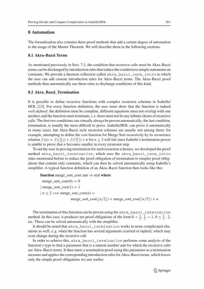
Proving Divide and Conquer Complexities in Isabelle/HOL 501
8 Automation
The formalisation also contains three proof methods that add a certain degree of automationto the usage of the Master Theorem. We will describe them in the following sections.
8.1 Akra–Bazzi Terms
As mentioned previously in Sect. 7.1, the condition that recursive calls must be Akra–Bazziterms canbedischargedby introduction rules that reduce the condition to simple statements onconstants. We provide a theorem collection called akra_bazzi_term_intro to whichthe user can add custom introduction rules for Akra–Bazzi terms. The Akra–Bazzi proofmethods then automatically use these rules to discharge conditions of this kind.
8.2 Akra_Bazzi_Termination
It is possible to define recursive functions with complex recursion schemes in Isabelle/HOL [13]. For every function definition, the user must show that the function is indeedwell-defined: the definition must be complete, different equations must not overlap with oneanother, and the functionmust terminate, i. e. theremust not be any infinite chains of recursivecalls. The first two conditions can virtually always be proven automatically; the last condition,termination, is usually the most difficult to prove. Isabelle/HOL can prove it automaticallyin many cases, but Akra–Bazzi style recursion schemes are usually not among them: forexample, attempting to define the cost function for Merge Sort recursively by its recurrencerelation f (n) = f ( n
2 )+ f ( n2 )+ n for n ≥ 2 will fail since Isabelle’s termination prover
is unable to prove that n becomes smaller in every recursion step.To aid the user in proving termination for such recursion schemes, we developed the proof
method akra_bazzi_termination, which uses the akra_bazzi_term_introrules mentioned before to reduce the proof obligation of termination to simpler proof oblig-ations that contain only constants, which can then be solved automatically using Isabelle’ssimplifier. A typical function definition of an Akra–Bazzi function then looks like this:
function merge_sort_cost::nat ⇒ real where
merge_sort_cost(0) = 0
| merge_sort_cost(1) = 1
| n ≥ 2 ⇒ merge_sort_cost(n) =merge_sort_cost(n/2) + merge_sort_cost(n/2) + n
The termination of this function can be proven using the akra_bazzi_terminationmethod. In this case, it produces ten proof obligations of the form 0 < 1
2 ,12 < 1, 0 ≤ 1
2 · 2,etc. These can be solved automatically with the simplifier.
It should be noted that akra_bazzi_termination works in more complicated situ-ations as well, e. g. when the function has several arguments (curried or tupled), which mayeven change during the recursive call.
In order to achieve this, akra_bazzi_termination performs some analysis of thefunction’s type to find a parameter that is a natural number and for which the recursive callsare Akra–Bazzi terms. It then starts a termination proof using this parameter as a terminationmeasure and applies the corresponding introduction rules for Akra–Bazzi terms, which leavesonly the simple proof obligations we saw earlier.
123
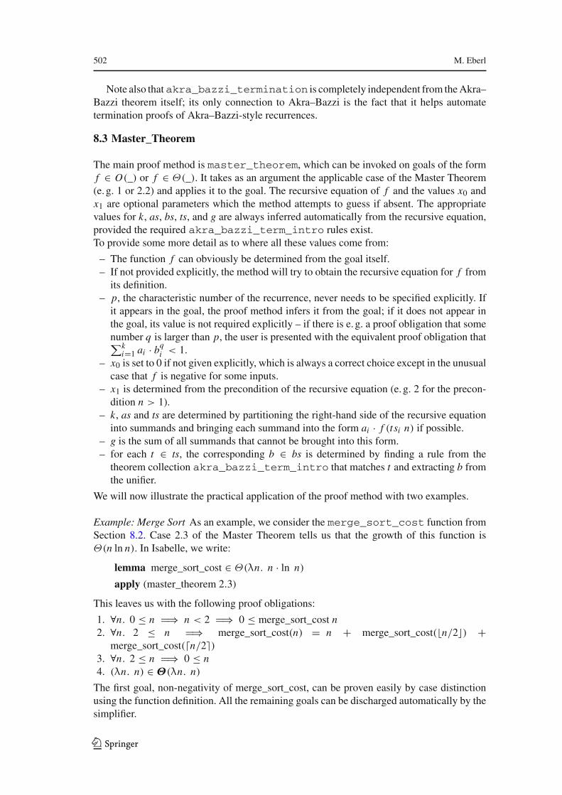
502 M. Eberl
Note also that akra_bazzi_termination is completely independent from theAkra–Bazzi theorem itself; its only connection to Akra–Bazzi is the fact that it helps automatetermination proofs of Akra–Bazzi-style recurrences.
8.3 Master_Theorem
The main proof method is master_theorem, which can be invoked on goals of the formf ∈ O(_) or f ∈ Θ(_). It takes as an argument the applicable case of the Master Theorem(e. g. 1 or 2.2) and applies it to the goal. The recursive equation of f and the values x0 andx1 are optional parameters which the method attempts to guess if absent. The appropriatevalues for k, as, bs, ts, and g are always inferred automatically from the recursive equation,provided the required akra_bazzi_term_intro rules exist.To provide some more detail as to where all these values come from:
– The function f can obviously be determined from the goal itself.– If not provided explicitly, the method will try to obtain the recursive equation for f from
its definition.– p, the characteristic number of the recurrence, never needs to be specified explicitly. If
it appears in the goal, the proof method infers it from the goal; if it does not appear inthe goal, its value is not required explicitly – if there is e. g. a proof obligation that somenumber q is larger than p, the user is presented with the equivalent proof obligation that∑k
i=1 ai · bqi < 1.
– x0 is set to 0 if not given explicitly, which is always a correct choice except in the unusualcase that f is negative for some inputs.
– x1 is determined from the precondition of the recursive equation (e. g. 2 for the precon-dition n > 1).
– k, as and ts are determined by partitioning the right-hand side of the recursive equationinto summands and bringing each summand into the form ai · f (tsi n) if possible.
– g is the sum of all summands that cannot be brought into this form.– for each t ∈ ts, the corresponding b ∈ bs is determined by finding a rule from the
theorem collection akra_bazzi_term_intro that matches t and extracting b fromthe unifier.
We will now illustrate the practical application of the proof method with two examples.
Example: Merge Sort As an example, we consider the merge_sort_cost function fromSection 8.2. Case 2.3 of the Master Theorem tells us that the growth of this function isΘ(n ln n). In Isabelle, we write:
lemma merge_sort_cost ∈ Θ(λn. n · ln n)
apply (master_theorem 2.3)
This leaves us with the following proof obligations:
1. ∀n. 0 ≤ n ⇒ n < 2 ⇒ 0 ≤ merge_sort_cost n2. ∀n. 2 ≤ n ⇒ merge_sort_cost(n) = n + merge_sort_cost(n/2) +
merge_sort_cost(n/2)3. ∀n. 2 ≤ n ⇒ 0 ≤ n4. (λn. n) ∈ Θ(λn. n)
The first goal, non-negativity of merge_sort_cost, can be proven easily by case distinctionusing the function definition. All the remaining goals can be discharged automatically by thesimplifier.
123

Proving Divide and Conquer Complexities in Isabelle/HOL 503
Example: Boncelet coding Another interesting example is given byDrmota and Szpankowski[8]: the average phrase length d(n) in Boncelet coding [6]. This is not related to Divide andConquer algorithms at all, but d does fulfil the Akra–Bazzi-type recurrence
d(n) = 1 + p · d(p · n + δ) + q · d(q · n − δ)where p ∈ (0; 1) is a probability, q = 1 − p , and δ > 0 , δ < 1 , 2p + δ < 2. Since ourMaster Theorem applies to this recurrence, we can use the master_theorem tactic:
lemma boncelet_phrase_length:
fixes p δ::realfixes d::nat ⇒ real
defines q ≡ 1 − p
assumes p ∈ (0; 1) and δ ∈ (0; 1) and 2 · p + δ < 2 and ∀n. d(n) ≥ 0
assumes ∀n≥2. d(n) = 1 + p · d(p · n + δ) + q · d(q · n + δ)shows d ∈ Θ(λx . ln x)
using assms by (master_theorem recursion: d_rec, simp_all)
This example is particularly interesting because here we do not have a concrete function thatwe defined ourselves, but prove a theorem for an entire class of functions satisfying a certainrecurrence. Since d is not a function-package function, we need to give master_theoremthe recurrence rule to use, but then, the lemma can be proven automatically again. Note alsothat we did not specify which case to use here; Isabelle implicitly backtracks over all possiblecases and succeeds in case 2.3. It should, however, be mentioned that the Θ-estimate is notvery useful in this case: as Drmota and Szpankowski elaborate, an analysis of the redundancyof the Boncelet scheme requires more precise asymptotics, like the ones they provide.
Further examples of complexity proofs for recurrences derived from the computationalcosts of Divide and Conquer algorithms such as Karatsuba’s multiplication algorithm fornatural numbers, Strassen’s algorithm for matrix multiplication, or the deterministicMedian-of-Medians selection algorithm can be found in the examples file of our entry in theArchive of Formal Proofs [9].All examples can be proven mostly automatically with themaster_theorem method and Isabelle’s simplifier. (in no small part thanks to the deci-sion procedure we presented in Sect. 3.2.2) There are only three kinds of subgoals that aresometimes left behind:
– Positivity/non-negativity for sufficiently large inputs; this can typically be shown bystraightforward induction and simplification.
– Showing that p satisfies∑k
i=1 asi · bspi = 1; proving this is usually automatic, but can
be non-trivial in some cases. One such example is that from our introduction: f (n) =f (n/4) + f (n/2) + 1 with p = log2 ϕ, where ϕ is the golden ratio.
– Inequalities like q < p for complicated constants p, q (e. g. involving logarithms andsquare roots); these can usually be proven automatically by approximation [12].
8.4 Akra_Bazzi_Approximation
In some of the cases of the Master Theorem, the goal contains the parameter p. As shownbefore, this p always exists and is unique. It can, however, not always be expressed in a closedform. One example for such a situation is the function f (x) = f (x/3) + f (3x/4), forwhich p seems to have no closed form, but can be approximated to 1.152.
123

504 M. Eberl
Our Master Theorem in Isabelle/HOL yields
lemma f ∈ Θ(λn. nakra_bazzi_exponent([1,1],[1/3,3/4]))
where akra_bazzi_exponent is a function that, given lists as and bs that fulfil the usualconditions, returns the unique p such that
∑ki=1 asi · bsp
i = 1.Of course, one would now like to obtain and verify at least an approximate value for
this exponent. An approximate value for p can be found e. g. using an external com-puter algebra system or by applying Newton’s method as described in Sect. 8.4. Oncesuch an approximation has been found, it can then be verified with our proof methodakra_bazzi_approximate:
lemma akra_bazzi_exponent([1, 1], [1/3, 3/4]) ∈ [1.1519623; 1.1519624]by (akra_bazzi_approximate 29)
This proof method internally uses the approximation tactic [12], which uses Taylorseries expansions, interval arithmetic, and reflection (i. e. Isabelle’s code generator [11])to certify bounds on the values of certain transcendental functions. The number 29 in theinvocation here indicates the precision (measured in binary digits) of the computation. If itis too low, the proof attempt might fail even though the statement is true; if it is too high, theproof will take more time. The user of the proof method should therefore find a precisionvalue that is as low as possible while still being high enough for the proof to succeed.
Likeakra_bazzi_termination, themethodakra_bazzi_approximation iscompletely orthogonal to theAkra–Bazzi theorem; neither depends on the other. In particular,no part of the proof of the Akra–Bazzi theorem relies on numerical approximation.
Approximating p As a side note: p can be approximated quite easily. Recall that p wasdefined as the unique real number such that t (p) = 1 where
t : R → R>0, x →k∑
i=1
ai · b xi .
Note that t (x) − 1 is convex and t ′(x) has no zeros. This means that Newton’s methodcan be used to approximate p very efficiently: Due to the convexity of t (x) − 1, a Newtonstep at any lower bound (i. e. intersecting the tangent of t at the lower bound with the x axis)will yield a better lower bound, and intersecting the secant of a lower bound and an upperbound on p with the x axis will yield a better upper bound. This can be used to obtain goodapproximation intervals for p very quickly.
As initial lower and upper bounds, one can e. g. use the estimates
− ln ak
ln bk≤ p ≤ − ln
(n · maxi∈[1;n] ai
)
ln(maxi∈[1;n] bi
) where k ∈ [1; n] arbitrary.
We have not verified this approximation algorithm in Isabelle, since the approximationcan easily be done externally in an unverified way and then certified using e. g. the akra_bazzi_approximation method.
123
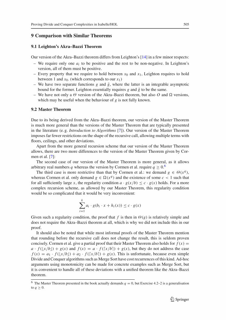
Proving Divide and Conquer Complexities in Isabelle/HOL 505
9 Comparison with Similar Theorems
9.1 Leighton’s Akra–Bazzi Theorem
Our version of the Akra–Bazzi theorem differs from Leighton’s [14] in a few minor respects:
– We require only one ai to be positive and the rest to be non-negative. In Leighton’sversion, all of them must be positive.
– Every property that we require to hold between x0 and x1, Leighton requires to holdbetween 1 and x0. (which corresponds to our x1)
– We have two separate functions g and g, where the latter is an integrable asymptoticbound for the former. Leighton essentially requires g and g to be the same.
– We have not only a Θ version of the Akra–Bazzi theorem, but also O and versions,which may be useful when the behaviour of g is not fully known.
9.2 Master Theorem
Due to its being derived from the Akra–Bazzi theorem, our version of the Master Theoremis much more general than the versions of the Master Theorem that are typically presentedin the literature (e. g. Introduction to Algorithms [7]). Our version of the Master Theoremimposes far fewer restrictions on the shape of the recursive call, allowing multiple terms withfloors, ceilings, and other deviations.
Apart from the more general recursion scheme that our version of the Master Theoremallows, there are two more differences to the version of the Master Theorem given by Cor-men et al. [7]:
The second case of our version of the Master Theorem is more general, as it allowsarbitrary real numbers q whereas the version by Cormen et al. require q ≥ 0.6
The third case is more restrictive than that by Cormen et al.: we demand g ∈ Θ(xq),whereas Cormen et al. only demand g ∈ (xq) and the existence of some c < 1 such thatfor all sufficiently large x , the regularity condition a · g(x/b) ≤ c · g(x) holds. For a morecomplex recursion scheme, as allowed by our Master Theorem, this regularity conditionwould be so complicated that it would be very inconvenient:
k∑
i=1
ai · g(bi · x + hi (x)) ≤ c · g(x)
Given such a regularity condition, the proof that f is then in Θ(g) is relatively simple anddoes not require the Akra–Bazzi theorem at all, which is why we did not include this in ourproof.
It should also be noted that while most informal proofs of the Master Theorem mentionthat rounding before the recursive call does not change the result, this is seldom provenconcisely. Cormen et al. give a partial proof that their Master Theorem also holds for f (x) =a · f (x/b) + g(x) and f (x) = a · f (x/b) + g(x), but they do not address the casef (x) = a1 · f (x/b) + a2 · f (x/b) + g(x). This is unfortunate, because even simpleDivide andConquer algorithms such asMerge Sort have cost recurrences of this kind. Ad-hocarguments using monotonicity can be made for concrete examples such as Merge Sort, butit is convenient to handle all of these deviations with a unified theorem like the Akra–Bazzitheorem.
6 The Master Theorem presented in the book actually demands q = 0, but Exercise 4.2–2 is a generalisationto q ≥ 0.
123

506 M. Eberl
10 Conclusion
We formally verified a very general version of the Akra–Bazzi method [1] with the theoremprover Isabelle/HOL. This enables users of Isabelle to obtain verified asymptotic bounds formany typical ‘Divide and Conquer’ recurrence relations. In the process of our formalisation,we found a missing case in Leighton’s original proof [14]. We also clarified some importantparts of the proof that Leighton does not address (such as the asymptotic inequalities andlifting the estimate for continuous recurrences to discrete ones) and slightly generalised thetheorem.
Based upon our formal proof of the Akra–Bazzi method, we also proved a generalisationof the well-known Master Theorem whose generality is somewhere between the ‘classic’Master Theorem and the Akra–Bazzi method, but with no additional cost compared to the‘classic’ Master Theorem. In particular, we thus accounted rigorously for any rounding inthe recursive calls, which is often neglected in informal proofs of the Master Theorem.
Additionally, we developed some automated proof methods that facilitate defining suchrecursive functions and working with our Master Theorem. We evaluated this machinery onsome standard textbook examples of Divide and Conquer algorithms (Merge Sort, Karatsubamultiplication, deterministic Median-of-Medians selection) and found that the complexityproofs were almost completely automatic.
Acknowledgements Tobias Nipkow and Johannes Hölzl commented on an early draft of this work. LouayBazzi made a very helpful suggestion that allowed us to fix the missing case in Leighton’s proof. We alsothank the anonymous reviewers for their helpful suggestions and insightful questions.
Appendix: The Class of Admissible Integrals
We will now provide a proof of our claim from Sect. 3.3 that any admissible integral mustcoincide with the Riemann integral for all piecewise-continuous functions. First of all, weshall state again what admissibility means formally: Consider an integral notion I. Formally,I consists of
– A functional I : RR × R2 → R that maps a function f and interval bounds a and b to
the I-integral of f from a to b, denoted by∫ b
aI
f (x) dx .
– A set I ⊆ RR × R
2, the set of I-integrable functions. We say that f is I-integrable on[a; b] if ( f, a, b) ∈ I.
For the remainder of this section, we will always indicate for every use of the integral signwhich notion of integration is meant by writing the name of the integral underneath theintegral as we did above.
Now assume that I fulfils the following four properties (which are the same that werestated in Sect. 3.3, but more formally):
∀a, b, c ∈ R. a ≤ b ∧ c ≥ 0 −→ ((λ x . c), a, b) ∈ I ∧∫ b
aI
cdx = c · (a − b) (9)
∀a, b, a′, b′ ∈ R. ∀ f ∈ RR. a ≤ a′ ≤ b′ ≤ b ∧ ( f, a, b) ∈ I −→ ( f, a′, b′) ∈ I (10)
123
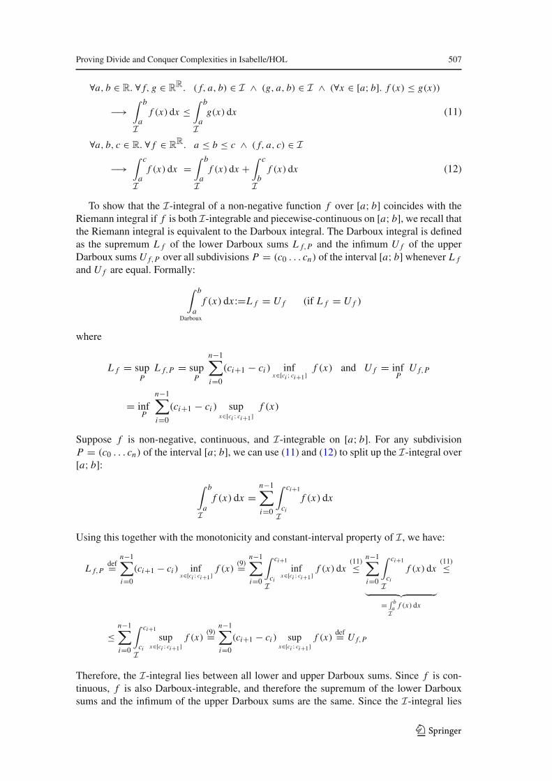
Proving Divide and Conquer Complexities in Isabelle/HOL 507
∀a, b ∈ R. ∀ f, g ∈ RR. ( f, a, b) ∈ I ∧ (g, a, b) ∈ I ∧ (∀x ∈ [a; b]. f (x) ≤ g(x))
−→∫ b
aI
f (x) dx ≤∫ b
aI
g(x) dx (11)
∀a, b, c ∈ R. ∀ f ∈ RR. a ≤ b ≤ c ∧ ( f, a, c) ∈ I
−→∫ c
aI
f (x) dx =∫ b
aI
f (x) dx +∫ c
bI
f (x) dx (12)
To show that the I-integral of a non-negative function f over [a; b] coincides with theRiemann integral if f is both I-integrable and piecewise-continuous on [a; b], we recall thatthe Riemann integral is equivalent to the Darboux integral. The Darboux integral is definedas the supremum L f of the lower Darboux sums L f,P and the infimum U f of the upperDarboux sums U f,P over all subdivisions P = (c0 . . . cn) of the interval [a; b] whenever L f
and U f are equal. Formally:
∫ b
aDarboux
f (x) dx :=L f = U f (if L f = U f )
where
L f = supP
L f,P = supP
n−1∑
i=0
(ci+1 − ci ) infx∈[ci ; ci+1]
f (x) and U f = infP
U f,P
= infP
n−1∑
i=0
(ci+1 − ci ) supx∈[ci ; ci+1]
f (x)
Suppose f is non-negative, continuous, and I-integrable on [a; b]. For any subdivisionP = (c0 . . . cn) of the interval [a; b], we can use (11) and (12) to split up the I-integral over[a; b]:
∫ b
aI
f (x) dx =n−1∑
i=0
∫ ci+1
ciI
f (x) dx
Using this together with the monotonicity and constant-interval property of I, we have:
L f,Pdef=
n−1∑
i=0
(ci+1 − ci ) infx∈[ci ; ci+1]
f (x)(9)=
n−1∑
i=0
∫ ci+1
ciI
infx∈[ci ; ci+1]
f (x) dx(11)≤
n−1∑
i=0
∫ ci+1
ciI
f (x) dx
︸ ︷︷ ︸= ∫ b
aI
f (x) dx
(11)≤
≤n−1∑
i=0
∫ ci+1
ciI
supx∈[ci ; ci+1]
f (x)(9)=
n−1∑
i=0
(ci+1 − ci ) supx∈[ci ; ci+1]
f (x)def= U f,P
Therefore, the I-integral lies between all lower and upper Darboux sums. Since f is con-tinuous, f is also Darboux-integrable, and therefore the supremum of the lower Darbouxsums and the infimum of the upper Darboux sums are the same. Since the I-integral lies
123

508 M. Eberl
inbetween, we have:∫ b
aDarboux
f (x) dxdef= L f = U f =
n−1∑
i=0
∫ ci+1
ciI
f (x) dx =∫ b
aI
f (x) dx .
We have therefore shown that I coincides with the Riemann integral on all continuous non-negative functions. Since we can split the I-integral of a piecewise-continuous functioninto a sum of I-integrals of continuous functions, this extends to all piecewise-continuousnon-negative functions.
However, this result does not extend to more general notions of integrals and integrability:For example, let us consider the following integral I: A function is I-integrable if it is aconstant function or if it is [Q] = (λ x . if x ∈ Q then 1 else 0), the indicator function of therational numbers. The value of the integral is defined as
∫ b
aI
c dx :=c · (b − a) and∫ b
aI
[Q] dx :=b − a
Then I fulfils all four properties, but unlike the Lebesgue/Bochner/Henstock–Kurzweil inte-gral, the I-integral of [Q] is non-zero on all non-empty intervals.
References
1. Akra,M., Bazzi, L.: On the solution of linear recurrence equations. Comput. Optim. Appl. 10(2), 195–210(1998). doi:10.1023/A:1018373005182
2. Avigad, J., Donnelly, K.: Formalizing O notation in Isabelle/HOL. In: Basin, D., Rusinowitch, M. (eds.)Automated Reasoning, Lecture Notes in Computer Science, pp. 357–371. Springer, Berlin (2004). doi:10.1007/978-3-540-25984-8_27
3. Avigad, J., Hölzl, J., Serafin, L.: A formally verified proof of the central limit theorem. CoRRabs/1405.7012 (2014). Presented at the Isabelle Workshop 2014
4. Ballarin, C.: Locales: a module system for mathematical theories. J. Autom. Reason. 52(2), 123–153(2014). doi:10.1007/s10817-013-9284-7
5. Bazzi, L., Mitter, S.K.: The solution of linear probabilistic recurrence relations. Algorithmica 36(1),41–57 (2003). doi:10.1007/s00453-002-1003-4
6. Boncelet Jr., C.G.: Block arithmetic coding for source compression. IEEE Trans. Inf. Theory 39(5),1546–1554 (1993). doi:10.1109/18.259639
7. Cormen, T.H., Leiserson, C.E., Rivest, R.L., Stein, C.: Introduction to Algorithms, 4th printing, 3rd edn.The MIT Press, Cambridge (2009)
8. Drmota, M., Szpankowski, W.: A Master theorem for discrete divide and conquer recurrences. J. ACM60(3), 16:1–16:49 (2013). doi:10.1145/2487241.2487242
9. Eberl, M.: The Akra–Bazzi Theorem and the Master Theorem. Archive of Formal Proofs (2015). http://www.isa-afp.org/entries/Akra_Bazzi.shtml, Formal proof development
10. Eberl, M.: Landau Symbols. Archive of Formal Proofs (2015). http://www.isa-afp.org/entries/Landau_Symbols.shtml, Formal proof development
11. Haftmann, F., Nipkow, T.: Code generation via higher-order rewrite systems. In: Blume, M., Kobayashi,N., Vidal, G. (eds.) Functional and Logic Programming. Lecture Notes in Computer Science, vol. 6009,pp. 103–117. Springer, Berlin (2010). doi:10.1007/978-3-642-12251-4_9
12. Hölzl, J.: Proving inequalities over reals with computation in Isabelle/HOL. In: Reis, G.D., Théry, L.(eds.) Proceedings of the ACM SIGSAM 2009 International Workshop on Programming Languages forMechanized Mathematics Systems (PLMMS’09), pp. 38–45. Munich (2009)
13. Krauss, A.: Automating Recursive Definitions and Termination Proofs in Higher-Order Logic. Ph.D. the-sis, Technische Universität München, Institut für Informatik (2009). http://nbn-resolving.de/urn/resolver.pl?urn:nbn:de:bvb:91-diss-20090722-681651-1-1
14. Leighton, T.: Notes on Better Master Theorems for Divide-and-Conquer Recurrences (1996). http://courses.csail.mit.edu/6.046/spring04/handouts/akrabazzi.pdf
123


C Analytic Number Theory
This chapter was originally published as an article in the proceedings of a peer-reviewedconference:
M. Eberl.Nine Chapters of Analytic Number Theory in Isabelle/HOL.In Interactive Theorem Proving. Leibniz International Proceedings in Informatics, 2019.DOI: 10.4230/LIPIcs.ITP.2019.16.
I am the sole author of this article, thus all contributions are mine.
Synopsis: This work consists of a formalisation of many basic concepts from the mathem-atical eld of Analytic Number Theory (including Dirichlet series, character theory, and theRiemann Z function). It then uses this as a basis for the formal proofs of some important the-orems, such as the Prime Number Theorem and Dirichlet’s Theorem. It covers most of Apostol’sclassic textbook Analytic Number Theory [3], sometimes going beyond the scope of the book.
This article is an open access publication and was published under a Creative Commons CC-BYlicence; it can therefore be redistributed freely. It is reproduced on the following pages in itspublished form.
99
Nine Chapters of Analytic Number Theory inIsabelle/HOLManuel EberlTechnical University of Munich, Boltzmannstraße 3, Garching bei München, Germanyhttps://www21.in.tum.de/[email protected]
AbstractIn this paper, I present a formalisation of a large portion of Apostol’s Introduction to AnalyticNumber Theory in Isabelle/HOL. Of the 14 chapters in the book, the content of 9 has been mostlyformalised, while the content of 3 others was already mostly available in Isabelle before.
The most interesting results that were formalised are:The Riemann and Hurwitz ζ functions and the Dirichlet L functionsDirichlet’s theorem on primes in arithmetic progressionsAn analytic proof of the Prime Number TheoremThe asymptotics of arithmetical functions such as the prime ω function, the divisor count σ0(n),and Euler’s totient function ϕ(n)
2012 ACM Subject Classification Mathematics of computing → Mathematical analysis
Keywords and phrases Isabelle, theorem proving, analytic number theory, number theory, arith-metical function, Dirichlet series, prime number theorem, Dirichlet’s theorem, zeta function, Lfunctions
Digital Object Identifier 10.4230/LIPIcs.ITP.2019.16
Supplement Material The proof developments in the Archive of Formal Proofs (AFP) that thiswork refers to are listed in the bibliography. Additionally, a precise overview of what material fromthe book has been formalised and which theorems in the book correspond to which theorems in theformalisation can be found at 10.5281/zenodo.3262266.
Funding This work was supported by DFG grant NI 491/16-1. Part of it was conducted during aresearch visit in collaboration with the ALEXANDRIA project (ERC grant 742178).
Acknowledgements I would like to thank John Harrison for doing all the incredibly hard work ofcreating an extensive library of complex analysis in HOL Light – the first of its kind – and LarryPaulson and Wenda Li for porting it to Isabelle/HOL and extending it even further. Without theseefforts, my work would not have been possible. Larry Paulson also started off the analytic proofof the Prime Number Theorem in Isabelle and allowed me to take over and replace it with a morehigh-level approach. I also thank Jeremy Avigad and Johannes Hölzl, who commented on a draft ofthis document, and the anonymous reviewers, who gave a number of helpful suggestions.
1 Introduction
The formalisation of Apostol’s book in Isabelle/HOL started from the simple desire to havemore properties about Euler’s ϕ function available in the system. However, Apostol’s styleturned out to be very amenable to formalisation, and the subject matter was both of greatinterest as a basis for further development of number theory in Isabelle and as a case studyfor Isabelle’s libraries on asymptotics and complex analysis. After 1.5 years of a highlypart-time one-person effort, most of the book (and quite a bit of material that goes beyondthe book) has been formalised:
© Manuel Eberl;licensed under Creative Commons License CC-BY
10th International Conference on Interactive Theorem Proving (ITP 2019).Editors: John Harrison, John O’Leary, and Andrew Tolmach; Article No. 16; pp. 16:1–16:19
Leibniz International Proceedings in InformaticsSchloss Dagstuhl – Leibniz-Zentrum für Informatik, Dagstuhl Publishing, Germany
16:2 Nine Chapters of Analytic Number Theory in Isabelle/HOL
Chapters 1, 5, and 9 consist of fairly basic material (e. g. GCDs, congruences, Quadraticreciprocity), most of which was already available in the Isabelle/HOL library.The results from Chapters 2, 3, 4, and 6 have been formalised in their entirety.Chapters 10, 11, and 12 have been formalised with some omissions.For Chapters 7 and 13 (Dirichlet’s Theorem and PNT), equivalent results have beenformalised using a different approach.Chapters 8 and 14 have been skipped. The former is being actively worked on; the latterconcerns number partitions and has little connection to the other material in the book.Various interesting results from other sources (e. g. Hildebrand’s lecture notes [21]) thatare not proven in Apostol’s book have also been formalised.
For more precise information on this, see the supplementary material listed before.I put particular focus on developing a usable library of Dirichlet series on one hand and
concrete results about the distribution of primes on the other. As the development is muchtoo large to be presented here in full, I will go through a high-level description of some ofthe most interesting material. Special attention will be given to parts where I encountereddifficulties or chose a different route than Apostol did in his book. Proofs will only be givenin the form of very brief sketches, e. g. when it is necessary in order to understand difficultiesin formalising them. I would like to refer readers who are interested in the actual proofs eitherto my commented formalisation in the Archive of Formal Proofs (AFP) [13, 12, 15, 18, 16] orto the numerous excellent textbooks and lecture notes on the subject [2, 21, 7]. I chose not toshow Isabelle code in this presentation since the main results are very close to mathematicalnotation (e. g. Re s ≥ 1 =⇒ s 6= 1 =⇒ zeta s 6= 0) and showing the Isabelle code wouldtherefore not provide much additional insight.
Let me now give an outline of the sections to follow: Section 2 lists related work. Section 3defines formal Dirichlet series and their connection to complex-analytic functions. Section 4introduces multiplicative characters and Dirichlet characters. Section 5 builds on the Dirichletseries library to treat various L functions, such as the famous Riemann ζ function. Section 6describes my formalisation of the Prime Number Theorem (PNT). Section 7 gives some moreexamples of interesting results that were formalised. Section 8 gives an overview of the size ofvarious parts of my formalisation and the effort involved in creating it. Lastly, in Section 9,some conclusions are drawn from this project.I Remark 1. Any sum
∑p or product
∏p is to be understood to run over prime p only.
2 Related Work
The first formalisation of a result related to this work was that of the PNT in Isabelle/HOLby Avigad et al. [5] in 2007. They formalised the elementary Selberg–Erdős proof.1 Carneiroformalised the same proof in Metamath [11].
Harrison developed the first (and until now only) formalisation of an analytic proof of thePNT in 3,600 lines [20] of HOL Light. He followed Newman’s presentation, which I also did.2
1 Unfortunately, this work was never submitted to the AFP and has not been maintained since then. Atthe time of writing this paper, the proofs are 12 years old; the formalisation comprises almost 27,000lines, and many of them are unstructured proof scripts. Bringing them up to date to work with amodern version of Isabelle would be a massive undertaking. However, much of the more general materialdeveloped by Avigad et al. was moved to Isabelle’s library, and for a considerable part of the remainingmaterial, equivalent results are now already a part of the Isabelle library or my work anyway.
2 Paulson later ported Harrison’s development to Isabelle/HOL, but the ported proofs were lengthy andnot very readable, so he and I decided that it would be better to redo them in a more high-level style,which I did. Only a few small lemmas were kept.
M. Eberl 16:3
Harrison also proved Dirichlet’s Theorem [19] and I used some of the high-level structure ofhis development as an inspiration for mine. Moreover, formalisations of Bertrand’s postulateexist by Harrison in HOL Light, by Théry in Coq [27], by Riccardi in Mizar [26], by Carneiroin Metamath [10], by Asperti and Ricciotti in Matita [4], and by Biendarra and Eberl inIsabelle/HOL [9].
The big difference between these formalisations and the present one is that this onecontains not just one result and the material required for it, but the majority of a textbookon the subject. Many proofs are much simpler and more “high-level” through the use ofDirichlet series and Isabelle’s advanced machinery for asymptotic reasoning.
3 Dirichlet Series
The central objects in analytic number theory are Dirichlet series. These are the main toolsthat set apart my approach to formalised number theory from that of previous formalisationwork in multiplicative number theory like that by Avigad et al., Harrison, and Carneiro.
I Definition 2 (Formal Dirichlet series). A formal series of the form f(s) =∑∞n=1 ann
−s iscalled a Dirichlet series. Typically, the an are real or complex (we will mostly look at thecomplex case). The Dirichlet series over R or C form a commutative ring with the obviouschoices for 0, 1, and addition. Multiplication is defined as (
∑∞n=1 ann
−s) · (∑∞n=1 bnn−s) =∑∞
n=1(∑k·l=n akbl)n−s . Also,
∑∞n=1 ann
−s has a multiplicative inverse iff a1 6= 0.
I Theorem 3 (Convergence of Dirichlet series). Each Dirichlet series has abscissæ of con-vergence σc and absolute convergence σa such that the infinite sum corresponding to it isabsolutely summable for Re(s) > σa, conditionally summable for Re(s) ∈ (σc, σa), anddivergent for Re(s) < σc (where Re(s) denotes the real part of s). The σc and σa satisfyσc ≤ σa ≤ σc + 1 and may be ±∞.
Much like formal power series (i. e. ordinary generating functions) for combinatorics,Dirichlet series are closely associated with number theory. Like generating functions, theyare of great interest as mere formal objects, but when they converge, their interpretation asa complex-valued function is also enormously useful, as we will see.
Various formal analogues of analytic operations can be defined for Dirichlet series e. g.reciprocal, derivative, integral, exp(f(s)), ln f(s), f(s+ s0), f(m · s), and subseries. Thesehave similar properties to their analytic counterparts (e. g. exp(f(s))′ = f ′(s) exp(f(s))) evenwhen they do not converge. When they do converge, they typically agree with their analyticcounterparts. This allows one to prove properties of the analytic functions by reasoning onthe formal level and vice versa.
There are 4,800 lines of material on formal Dirichlet series in my formalisation. This isfar too much to show here, so I simply say that it contains all of Chapter 11 in Apostol’sbook and more, except for Sections 11.10 and 11.11. I will only show a few small examplesthat illustrate the aforementioned interplay of the formal and the analytical level:
One example of using formal Dirichlet series to derive an analytic result is this:
I Theorem 4. Let ω(n) be the number of distinct prime factors of n and µ(n) the Möbius µfunction, i. e. (−1)ω(n) if n is square-free and 0 otherwise. Then
∑∞n=1 µ(n)/n2 = 6/π2 .
Proof. Consider the formal series ζ(s) :=∑∞n=1 n
−s and M(s) :=∑∞n=1 µ(n)n−s. It is clear
that they both converge absolutely for Re(s) > 1 by the comparison test. It is easy to show∑d|n µ(d) = [n = 1], i. e. ζ(s)M(s) = 1 holds formally [2]. Thus, it also holds analytically
for Re(s) > 1 so that we have ζ(2)M(2) = 1 and therefore M(2) = 1/ζ(2), where ζ(2) – thefamous Basel problem – has the well-known value π2/6 [6]. J
ITP 2019
16:4 Nine Chapters of Analytic Number Theory in Isabelle/HOL
The following theorem allows us to transfer an analytic equality to the formal level:
I Theorem 5 (Uniqueness of Dirichlet series). Let f(s), g(s) be two formal Dirichlet serieswhose abscissa of convergence is <∞. If there exists a sequence sk with Re(sk) −→∞ and∀k. f(sk) = g(sk), then f(s) and g(s) are equal as formal Dirichlet series.
I Remark 6. In Isabelle, the condition on the existence of the sequence sk is replaced by thefollowing equivalent and more concise formulation using filters [22]:
∃F s in Re going-to at-top. f(s) = g(s)
The filter “f going-to F ” is the contravariant image of F under f , i. e. “Re going-to at-top”describes the neighbourhood of complex numbers with “sufficiently large” real part.
The “∃F x in F. P (x)” notation stands for “P (x) holds frequently in F ”, i. e. the comple-ment of P is not in the filter F . Less formally, one could say that P (x) holds “again andagain”. In the case of “Re going-to at-top”, this means that for any C ∈ R, there exists ans with Re(s) ≥ C for which the property is fulfilled.
I Definition 7 (Truncation operator). For a Dirichlet series f(s) =∑∞n=1 ann
−s, letTm(f(s)) =
∑mn=1 ann
−s denote the m-th order truncation of f(s). The result is a Di-richlet polynomial, i. e. a Dirichlet series with only finitely many non-zero coefficients.
I Theorem 8. f(s) = g(s)←→ ∀m. Tm(f(s)) = Tm(g(s)).
The following is an instance where these theorems are used to avoid a lot of complicatedreasoning on the formal level by leveraging a result on the analytic level:
I Theorem 9. For any (not necessarily convergent) Dirichlet series f(s) and g(s), we haveexp(f(s) + g(s)) = exp(f(s)) exp(g(s)) .
Proof. It is clear that the result holds analytically whenever the series converge, so if theseries have a non-empty half-plane of convergence, they must be equal by Theorem 5. Thequestion is how to show this if we do not know whether the series converge anywhere.
The key is to use Theorem 8 together with Tm(exp(h(s))) = Tm(exp(Tm(h(s)))). Thisallows us to assume w. l. o. g. that the series in question are Dirichlet polynomials andtherefore converge everywhere. J
I Remark 10. This technique of showing an equality on Dirichlet series by showing thatit holds for all Dirichlet polynomials works if the two sides of the equation in question arecontinuous functions w. r. t. the topology on formal Dirichlet series, i. e. each coefficient ofthe result only depends on finitely many coefficients of the input. The topological structureof Dirichlet series was not formalised yet, but this is a useful fact to keep in mind.
The following is another important theorem connecting a series with the function itdefines that we will use later:
I Theorem 11 (Pringsheim–Landau). Let f(s) be a Dirichlet series with non-negative realcoefficients and σa 6= ±∞. Then f(s) has a singularity at σa.
Conversely, if f(s) has an an analytic continuation to some half-plane s | Re(s) > c ,then σa ≤ c. In particular, if f(s) is entire, the series must converge everywhere.

M. Eberl 16:5
4 Characters of a Finite Abelian Group
The next concept we shall explore is that of a multiplicative character, which will be neededto prove Dirichlet’s theorem. For this section, let G = (G, ·, 1) be a finite abelian group.
IDefinition 12 (Multiplicative character). A character is a group homomorphism χ : G→ C×,i. e. χ(1) = 1 and χ(a · b) = χ(a)χ(b) for any a, b ∈ G. The character χ0 that maps everyelement to 1 is called the principal character.
For the necessary group theory, I use the HOL-Algebra library by Ballarin, which models agroup as a record containing entries for the operation ·, the neutral element 1, and an explicitcarrier set (which does not have to be the full type universe). The latter is necessary in HOLbecause notions such as subgroups cannot easily be expressed without explicit carrier sets.The fact that such a record indeed describes a group is then formalised as a locale [8] calledgroup, which fixes such a record and assumes that all the usual group axioms hold.
A character can then be defined as a locale that extends the group locale by fixing afunction χ :: α → C (where α is the type of the group elements) and assuming that thetwo homomorphism properties mentioned above hold for χ. For convenience, I only assumeχ(1) 6= 0 (from which χ(1) = 1 easily follows) and I additionally require χ(x) = 0 for any xnot in the carrier of the group. The latter is to ensure extensionality, i. e. two characters areequal as HOL values iff they return the same result on every group element.
I Definition 13 (Pontryagin dual group). Denote the set of characters of G by G. Then Gforms a group G := (G, ·, χ0) with point-wise multiplication and χ0 as the identity. Thisgroup is called the Pontryagin dual group of G.
I Theorem 14 (Number of characters). |G| = |G|
In Isabelle, the proof is by induction on the subgroups of G, using a custom induction ruleinspired by Apostol’s proof. The idea here is to successively “adjoin” elements, i. e. for asubgroup H and some x ∈ G \H, we form 〈H;x〉, the subgroup generated by H ∪ x:
I Lemma 15 (Induction on a group). Let G = (G, ·, 1) be a group and H some subgroup ofG. Let P be some property on groups. If P (H) holds and P (H ′) implies P (〈H ′;x〉) for allsubgroups H ′ ⊇ H and all x ∈ G \H ′, then P (G) holds.
I use this to show a stronger version of Theorem 14 that is just as easy to show:
I Theorem 16 (Number of character extensions). Let H be a subgroup of G and χ ∈ H. Let
C(G) := χ′ ∈ G | ∀x∈H. χ′(x) = χ(x)
denote the set of characters on G that agree with χ on H. Then |C(G)| · |H| = |G| , i. e.there are precisely |G|/|H| ways to extend a character on H to a character on G.
Proof. By straightforward induction according to Lemma 15, using the bijection
f : C(〈H ′;x〉) → C(H ′)× z ∈ C | zn = 1, f(χ) = (y 7→ χ(y), χ(x))
in the induction step. J
Theorem 14 follows directly by taking H = (1, ·, 1). Another useful corollary is this:
I Corollary 17. For any x 6= 1, there exists a χ ∈ G such that χ(x) 6= 1.
ITP 2019
16:6 Nine Chapters of Analytic Number Theory in Isabelle/HOL
With this, we can prove a nice property that Apostol does not cover at all:
I Theorem 18 (Isomorphism to the double dual). G is isomorphic to its double dual via thenatural isomorphism ν : G→ G , ν(x) = (χ 7→ χ(x)) .
This isomorphism is useful for the next properties:
I Theorem 19 (Orthogonality relations). For any χ ∈ G resp. x ∈ G, we have:
∑
x∈Gχ(x) =
|G| if χ = χ0
0 otherwise(1)
∑
χ∈G
χ(x) =|G| if x = 10 otherwise
(2)
Apostol’s proof for (1) is very simple and straightforward to formalise. In order to show(2) from (1), Apostol represents the set of characters of G as a character table of G, i. e. a|G|×|G| complex matrix. If we denote this matrix by A, (1) shows that AA∗ = nI (where A∗is the conjugate transpose of A). By simple linear algebra, A∗A = nI and thus (2) follows.
Formalising this argument would have required importing Isabelle’s linear algebra libraryand doing some tedious work to relate the matrix to the characters, so I chose another route:One could prove (2) relatively easily using the same induction principle as before in about 70lines, but the easiest way is to simply use Pontryagin duality: (2) is, in fact, nothing but thedual of (1), with G for G and ν(x) for χ. This requires only 6 lines of Isabelle code.
I Definition 20 (Dirichlet character). A Dirichlet character χ for the modulus m ∈ N>1 isa character of the multiplicative group of the residue ring Z/mZ. For convenience, χ isrepresented as a periodic function of type N→ C with period m, i. e. χ(k) = χ(k mod m).
I Remark 21. Apostol’s and my treatment of characters are quite elementary. Thereis an alternative, more group-theoretic view on this: It is straightforward to show thatG1×G2 ' G1 × G2 and that Cn ' Cn for cyclic groups Cn. Together with the FundamentalTheorem of Finite Abelian Groups, this implies a stronger variant of Theorem 14, namelyG ' G. However, unlike with G ' G, the isomorphism is not natural and establishing itindeed requires the Fundamental Theorem, which is currently not available in HOL-Algebra.Since the formal proofs that were presented in this section are still reasonably short, I do notthink this is a big problem.
5 The L Functions
In this section, we will look at four functions from the class of L functions: Riemann’s ζfunction, Dirichlet’s L function, Hurwitz’s ζ function, and the periodic ζ function. These areall complex-valued functions that are defined by an infinite sum for Re(s) > 1 and can beanalytically or meromorphically continued to the entire complex plane.
I Definition 22 (Riemann’s ζ function). For Re(s) > 1, the Riemann ζ function is given bythe Dirichlet series ζ(s) =
∑∞n=1 n
−s .
I Definition 23 (Dirichlet L functions). Let χ be a Dirichlet character for the modulus m > 0.Then L(s, χ) is given by the Dirichlet series L(s, χ) =
∑∞n=1 χ(n)n−s for Re(s) > 1 if χ = χ0
and for Re(s) > 0 if χ 6= χ0.
We immediately get the following properties for free from the Dirichlet series library:

M. Eberl 16:7
I Theorem 24. Let Λ(n) denote the von Mangoldt function. Then, if Re(s) > 1:
ζ(s) =∏
p
11− p−s ζ ′(s) = −
∞∑
n=1
lnnns
ln ζ(s) =∞∑
n=2
Λ(n)lnn · ns
L(s, χ) =∏
p
11− χ(p)p−s L′(s, χ) = −
∞∑
n=1
χ(n) lnnns
lnL(s, χ) =∞∑
n=2
χ(n)Λ(n)lnn · ns
However, ζ(s) and L(s, χ) can be defined on a larger domain:
I Theorem 25 (Analytic continuation of ζ(s) and L(s, χ)).1. ζ(s) can be continued to an analytic function on C \ 1 with a simple pole at s = 1.2. For non-principal χ, L(s, χ) can be continued to an entire function.3. For χ = χ0, we have L(s, χ0) = ζ(s) ·∏p|m(1− p−s) , i. e. L(s, χ0) is equal to ζ(s) up to
an entire factor and is therefore also analytic on C \ 1 with a simple pole at s = 1.
The difficult part here is to actually construct the analytic continuations. To do thisuniformly and without duplication of work, Newman uses a generalisation of ζ(s):
I Definition 26 (Hurwitz’s ζ function). Let a ∈ R>0 and Re(s) > 1. Then ζ(s, a) is given bythe (non-Dirichlet) series ζ(s, a) =
∑∞n=0 (n+ a)−s .
Apostol only considers ζ(s, a) for a ∈ (0, 1] since some results only hold for a ≤ 1 and thecase of a > 1 can be reduced to a ∈ (0, 1]. It is, however, useful to allow also a ≥ 1 – e. g. inNewman’s proof of the PNT, as noted already by Harrison [20].
B Claim 27. ζ(s, a) can be continued analytically to C \ 1 with a simple pole at s = 1.Both Riemann’s ζ function and the Dirichlet L functions can easily be expressed in terms ofζ(s, a), so that a continuation for Hurwitz’s ζ also yields continuations for the other two [2].
The main question now is therefore how to construct the continuation of ζ(s, a).
5.1 Analytic Continuation of Hurwitz’s ζ FunctionApostol constructs the continuation using an integral along an infinite contour. I did formalisethis eventually (see Theorem 36), but when I first defined ζ(s, a) in Isabelle, this approachseemed quite daunting to me, so I chose another route that seems to be folklore [2, 24] andthat I discovered independently: Since ζ(s, a) is defined for Re(s) > 1 by an infinite sum∑∞n=0(n+ a)−s and the corresponding improper integral
∫∞0 (x+ a)−s dx is easy to compute,
the Euler–MacLaurin summation formula [14] suggests itself. Applying it, we obtain
∞∑
n=0(s+ a)−n − a1−s
s− 1 = a−s
2 +N∑
i=1
B2i(2i)! a
−s−2i+1s2i−1 +
(−1)2Ns2N+1
(2N + 1)!
∫ ∞
0P2N+1(t) · (t+ a)−s−2N−1 dt (3)
where sk denotes the rising factorial, Bk is the k-th Bernoulli number, and Pk(t) is theperiodic version of the Bernoulli polynomial Bk(t), i. e. Pk(t) = Bk(t− btc).
The right-hand side is now actually analytic on a larger domain: all terms except the lastone are clearly entire functions in s; the only non-obvious term is the integral in the lastsummand. Leibniz’s rule shows that the definite integral
∫ b0 is analytic in s, and an integral
version of the Weierstraß M -test then shows that the improper integral∫∞
0 is uniformlyconvergent and therefore analytic in s for Re(s) > −2N .
ITP 2019

16:8 Nine Chapters of Analytic Number Theory in Isabelle/HOL
Let us write prezetaN (s, a) for the right-hand side. This is then a function in s that isanalytic for Re(s) > −2N and that also fulfils
prezetaN (s, a) =∞∑
n=0(s+ a)−n − a1−s
s− 1 for Re(s) > 1 .
This means that two functions prezetaM and prezetaN will always agree on Re(s) > 1, andby analytic continuation they will then also agree on their entire domain, i. e. for all s withRe(s) > −2max(M,N). We can therefore define a full analytic continuation to all of C bychoosing N “big enough” for each input, i. e. we define:
prezeta(s, a) := prezetamax(0,1−dRe(s)/2e)(s, a)
This function is entire and agrees with any of the prezetaN (s, a) for all s with Re(s) > −2N .Thus, it is an analytic continuation of the left-hand side of (3) so that we can simply define
ζ(s, a) := prezeta(s, a) + a1−s
s− 1
to obtain the Hurwitz ζ function on all of C \ 1. For convenience, I choose ζ(1, a) = 0 as isoften done in HOL-based systems (cf. Γ(−n) for n ∈ N in Isabelle/HOL and HOL Light).The advantage of the Euler–MacLaurin approach is that it is simple to implement becauseall of the “heavy lifting” has already been done in the AFP entry on the Euler–MacLaurinformula.
Various basic properties of the Hurwitz and Riemann ζ functions then follow in astraightforward way, of which I show some notable ones here:
I Theorem 28 (Special values of ζ). For any n ∈ N≥0, we have:
ζ(a,−n) = −Bn+1(a)n+ 1 ζ(−n) = −Bn+1
n+ 1 ζ(2n) = (−1)n+1 ·B2n · (2π)2n
2(2n)!
where Bn = Bn(1) are the Bernoulli numbers with B1 = 12 . In particular, this implies the
famous ζ(−1) = − 112 and the Basel problem ζ(2) = π2/6.
I Theorem 29 (Integral representation for ζ(s, a)). For any s with Re(s) > 1, we have:
Γ(s)ζ(s, a) =∫ ∞
0
ts−1e−at
1− e−t dt
5.2 The Non-Vanishing of ζ(s) and L(s, χ) for Re(s) = 1The following is a core ingredient in the Prime Number Theorem and Dirichlet’s Theorem:
I Theorem 30. For any s with Re(s) ≥ 1, we have ζ(s) 6= 0 and L(s, χ) 6= 0.
The case of Re(s) > 1 is a simple consequence of the Euler product formula for ζ(s) andL(s, χ) (cf. Theorem 24); the difficult part is the case Re(s) = 1. For this, I formalised thevery simple proof presented by Newman [25], whose key ingredient is the aforementionedPringsheim–Landau theorem (see Theorem 11). This proof is stunningly short and itshigh-level reasoning translates well to Isabelle/HOL now that a library of Dirichlet series isavailable. The gain is most striking for the Dirichlet L function, where Apostol’s proof onlytreats the case of s = 1, and even that proof is still more complicated than Newman’s and
M. Eberl 16:9
involves lengthy complicated “Big-O” reasoning. Indeed, in a first version of the formalisation,I formalised Apostol’s proof, but it was considerably longer and messier than the new version– with the added bonus that the new one is also more general.
Harrison also only proves L(1, χ) 6= 0 – indeed, he does not define L(s, χ) at all; hedefines only L(1, χ) since that is all that is required for Dirichlet’s theorem. Despite this andthe much higher verbosity of structured Isabelle proofs compared to HOL Light,his proof islonger than mine. The reason for this is that his proof is very elementary and uses very littlelibrary material while mine builds on a large library of Dirichlet series. However, I thinkthat the comparison is still not entirely unjustified since all of this material is sufficientlygeneral to be called “library material” (as opposed to technical lemmas specifically designedfor this one proof), and building sufficiently large and general libraries to make proofs likethis cleaner and easier is, after all, one of our goals in formalisation.
5.3 Hurwitz’s FormulaMore as a challenge to myself and the Isabelle libraries, I chose to formalise another non-trivialproperty of the ζ functions:
I Theorem 31 (Reflection formula for ζ(s)). For s /∈ 0, 1, we have:
1Γ(s) · ζ(1− s) = 2(2π)−s cos(πs/2)ζ(s)
Note that while Γ(s) has poles at s ∈ Z≤0, its reciprocal 1/Γ(s) is entire, so the formula holdseven for s ∈ Z<0.
This formula is a corollary of a more general one for ζ(s, a) known as Hurwitz’s formula:
I Theorem 32 (Hurwitz’s formula). Let a ∈ (0, 1) and s ∈ C \ 0 with a 6= 1 ∨ s 6= 1. Then:
1Γ(s) · ζ(1− s, a) = (2π)−s
(i−sF (s, a) + isF (s,−a)
)
Here, F (s, a) is the periodic ζ function, which we still have to define:
I Definition 33 (Periodic ζ function). For Re(s) > 1, the periodic ζ function F (s, a) is givenby the Dirichlet series F (s, a) =
∑∞n=1 e
2iπnan−s .
B Claim 34. F (s, a) is called periodic because F (s, a+ n) = F (s, a) for any integer n. Fornon-integer a, the above series converges for Re(s) > 0 and can be continued to an entirefunction. For integer a, it is simply the Riemann ζ function.
Apostol does not discuss the analytic continuation of F (s, a) at all, but it seemed usefulto me to do this nonetheless. The strategy I used to construct the continuation of F (s, a) fornon-integer a is somewhat interesting: Theorem 32 can be rearranged to give a formula thatexpresses F (s, a) in terms of ζ(1− s, a) and ζ(1− s, 1− a):
I Theorem 35. Let a ∈ (0, 1) and s ∈ C \ N. Then:
F (s, a) = i(2π)s−1Γ(1− s)(i−sζ(1− s, a)− isζ(1− s, 1− a)
)
We therefore proceed like this (assuming w. l. o. g. a ∈ (0, 1)):1. Show Theorem 32 for Re(s) > 1 (where F is simply given by its Dirichlet series).2. Use this to show Theorem 35 for Re(s) > 1.
ITP 2019
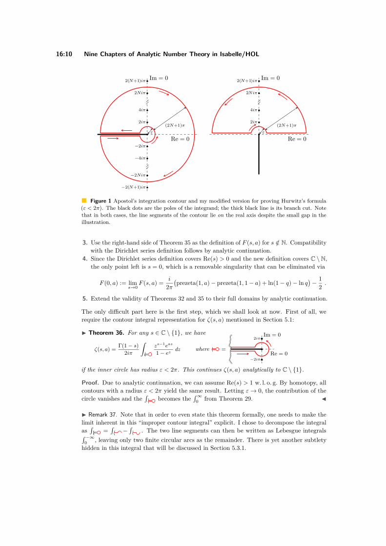
16:10 Nine Chapters of Analytic Number Theory in Isabelle/HOL
Re = 0
Im = 0
(2N+1)πε
2iπ
4iπ
2Niπ
2(N+1)iπ
−2iπ
−4iπ
−2Niπ
−2(N+1)iπ
Re = 0
Im = 0
(2N+1)πε
2iπ
4iπ
2Niπ
2(N+1)iπ
Figure 1 Apostol’s integration contour and my modified version for proving Hurwitz’s formula(ε < 2π). The black dots are the poles of the integrand; the thick black line is its branch cut. Notethat in both cases, the line segments of the contour lie on the real axis despite the small gap in theillustration.
3. Use the right-hand side of Theorem 35 as the definition of F (s, a) for s /∈ N. Compatibilitywith the Dirichlet series definition follows by analytic continuation.
4. Since the Dirichlet series definition covers Re(s) > 0 and the new definition covers C \ N,the only point left is s = 0, which is a removable singularity that can be eliminated via
F (0, a) := lims→0
F (s, a) = i
2π(prezeta(1, a)− prezeta(1, 1− a) + ln(1− q)− ln q
)− 1
2 .
5. Extend the validity of Theorems 32 and 35 to their full domains by analytic continuation.
The only difficult part here is the first step, which we shall look at now. First of all, werequire the contour integral representation for ζ(s, a) mentioned in Section 5.1:
I Theorem 36. For any s ∈ C \ 1, we have
ζ(s, a) = Γ(1− s)2iπ
∫zs−1eaz
1− ez dz where =Re = 0
Im = 02iπ
−2iπ
if the inner circle has radius ε < 2π. This continues ζ(s, a) analytically to C \ 1.
Proof. Due to analytic continuation, we can assume Re(s) > 1 w. l. o. g. By homotopy, allcontours with a radius ε < 2π yield the same result. Letting ε→ 0, the contribution of thecircle vanishes and the
∫becomes the
∫∞0 from Theorem 29. J
I Remark 37. Note that in order to even state this theorem formally, one needs to make thelimit inherent in this “improper contour integral” explicit. I chose to decompose the integralas∫
=∫
−∫
. The two line segments can then be written as Lebesgue integrals∫ −∞0 , leaving only two finite circular arcs as the remainder. There is yet another subtletyhidden in this integral that will be discussed in Section 5.3.1.

M. Eberl 16:11
The proof of Hurwitz’s formula for Re(s) > 1 then proceeds by computing this contourintegral in a different way using the Residue Theorem. To do this, we first need to approximateit by an integral over a finite contour CN,ε such that
∫CN,ε−→
∫as N → ∞. Figure 1
shows Apostol’s choice for CN,ε. Applying the Residue Theorem to this, we get
12iπ
∫
CN,ε
z−seaz
1− ez dz =∑
z0
indCN,ε(z0) Res
z=z0
z−seaz
1− ez (4)
where the sum on the right-hand side extends over all the singularities of the integrand(represented by black dots in Figure 1). We can now let N →∞ so that the contribution of theouter circle vanishes. The integral on the left-hand side is then simply a
∫, which is equal
to ζ(s, a)/Γ(s) by Theorem 36, and winding number on the right-hand side −1 for every non-zero pole z0. Evaluating this sum, we find that it indeed equals i−s
(2π)sF (s, a) + is
(2π)sF (s,−a),which concludes the proof of Hurwitz’s formula for Re(s) > 1. y
The formalisation of the proof was fairly routine. It is, however, quite large and tedious,containing almost 1,000 lines of proof code compared to 6.5 pages in Newman’s book (bothincluding the proof of Theorem 36). This seems to be a common pattern in Isabelle proofsusing the Residue Theorem and it is likely due to the many side conditions that need tobe shown, many of which are of geometric nature and thus much easier to explain to ahuman than to a theorem prover. Side conditions like the analyticity of the integrand, on theother hand, can be solved mostly automatically using Isabelle’s general-purpose automationtogether with specialised theorem collections like analytic_intros.
Some aspects of the formal proofs of these statements deserve more attention, and wewill discuss them now.
5.3.1 Branch CutsIn both theorems, the term z−s is a multi-valued function. It is defined in Isabelle as e−s ln z
where ln is the standard branch of the logarithm, which has a branch cut on the negativereal axis. The two lines of Apostol’s contour lie directly on this cut, taking different branchesof the logarithm (indeed, if they did not, they would simply cancel each other). This makessense formally when considering the integrand as a multi-valued function in the sense of aRiemann surface, but we do not have any of this analytic machinery in Isabelle.
My first idea to circumvent this problem was to resort to some kind of limiting argumentby placing the two horizontal lines not directly on the real axis, but some ε above (resp.below) it. However, this would likely have been a very tedious argument to do in Isabelle. Itherefore decided to again cut the contour into two halves, similarly to Remark 37. Whentheir integrals are added together, we recover Apostol’s contour integral. Due to symmetry,it is actually again enough to look at the upper half (cf. the right part of Figure 1), as thelower one follows by conjugation.
For this upper contour , we can now integrate over the same branch of the logarithmeverywhere. In order to avoid the branch cut of the standard logarithm, I use a differentbranch ln z := ln(−iz) + 1
2 iπ , whose branch cut lies on the negative imaginary axis, safelyaway from our contour. I also reversed the contour so that the winding numbers are all 1.
5.3.2 HomotopyThe proof of Theorem 36 uses the fact that the integral along is invariant for all radiiε < π. This is because all of these contours are homotopic, i. e. they can be continuouslydeformed into one another without crossing any of the singularities of the integrand. However,proving that this is the case turned out to be very tedious in Isabelle because there arealmost no library theorems that help showing that two composite paths are homotopic.
ITP 2019

16:12 Nine Chapters of Analytic Number Theory in Isabelle/HOL
I circumvented this problem in the following way: First of all, I restricted myself toε < π.3 Next, since the line segments extending from −π to −∞ are the same for all ε, wecan ignore them and focus on the finite subcontour . It can be seen that
∫=∫−∫
.By symmetry, it is enough to show that
∫is invariant under changes of ε. This, on the
other hand, is actually a corollary of (4): If we let N := 0, the sum on the right-hand sidevanishes so that we get
∫C0,ε
=∫
= 0 for all ε. Since∫
=∫−∫
= −∫
and(a half circle of radius π) is independent of ε, it follows that
∫is indeed the same for all ε.
Effectively, this replaces the homotopy argument (which is intuitively obvious for humansand not mentioned at all by Apostol) with a much “heavier” invocation of the ResidueTheorem – but since we already applied the Residue Theorem anyway, all that work isalready done.
5.3.3 Winding Numbers
The evaluation of the winding numbers indCN,ε(z0) is also easy for a human: the contour
CN,ε = clearly winds counter-clockwise once around each pole 2niπ with 0 < n ≤ N ,and all the other poles are clearly completely outside the contour. Proving these thingsin a theorem prover, on the other hand, is notoriously difficult [20], especially for a morecomplicated contour like this.
To show that the poles outside the contour really do lie outside (i. e. have winding number0), I use simple geometric arguments: for the branch cut on the negative imaginary axis,one can draw a vertical line from each point to −i∞ without crossing CN,ε, so the windingnumber for these points must be 0. Moreover, CN,ε is contained in a ball of radius (2N + 1)π,which is a convex set that does not contain any of the poles with n > N . Thus, these polesmust also have winding number 0.
The more difficult part is to show that the winding number for the points inside thecontour is 1. Geometric arguments for this are difficult. One approach would be to showthat the contour is a closed simple curve (which implies that the winding number must beeither -1, 0, or 1) and then weigh the contributions of the four different parts of the curve toshow that the overall value must be positive, thus 1. However, to avoid having to do thiswork, I instead use Li’s framework for computing winding numbers in Isabelle [23]. It isbased on computing Cauchy indices and comes with some setup to handle combinations ofline segments and circular arcs almost automatically, allowing me to prove that the windingnumbers are 1 with a mere 18 lines of proof code.
6 The Prime Number Theorem
The formal statement of the PNT is simply the asymptotic estimate π(x) ∼ x ln x, whereπ(x) is the number of prime numbers ≤x. I will now explain, in a high-level way, how theformalised proof works. First of all, let us define the following functions related to primes:
3 This restriction could easily be lifted by allowing arbitrary radii in (4) instead of just (2N + 1)π.
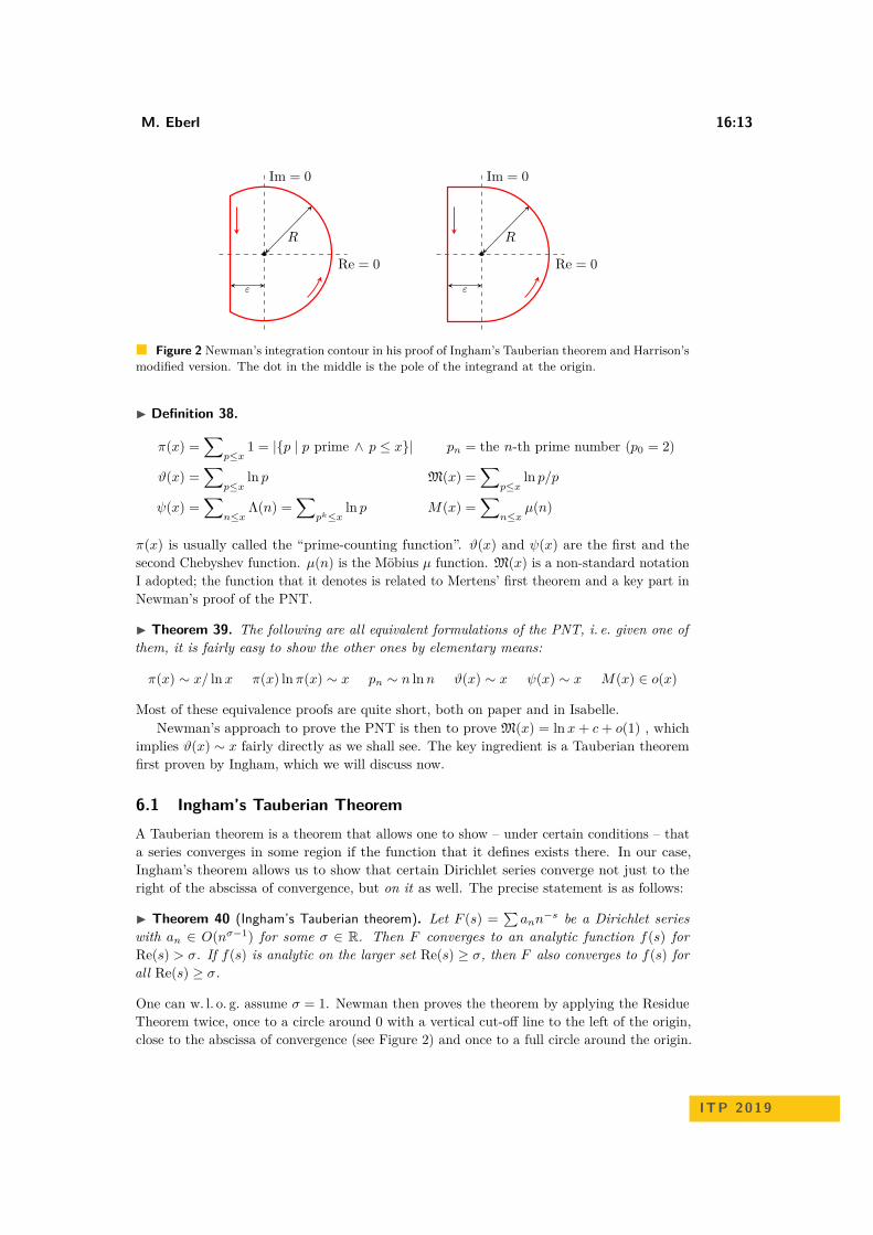
M. Eberl 16:13
Re = 0
Im = 0
R
ε
Re = 0
Im = 0
R
ε
Figure 2 Newman’s integration contour in his proof of Ingham’s Tauberian theorem and Harrison’smodified version. The dot in the middle is the pole of the integrand at the origin.
I Definition 38.
π(x) =∑
p≤x1 = |p | p prime ∧ p ≤ x| pn = the n-th prime number (p0 = 2)
ϑ(x) =∑
p≤xln p M(x) =
∑p≤x
ln p/p
ψ(x) =∑
n≤xΛ(n) =
∑pk≤x
ln p M(x) =∑
n≤xµ(n)
π(x) is usually called the “prime-counting function”. ϑ(x) and ψ(x) are the first and thesecond Chebyshev function. µ(n) is the Möbius µ function. M(x) is a non-standard notationI adopted; the function that it denotes is related to Mertens’ first theorem and a key part inNewman’s proof of the PNT.
I Theorem 39. The following are all equivalent formulations of the PNT, i. e. given one ofthem, it is fairly easy to show the other ones by elementary means:
π(x) ∼ x/ ln x π(x) ln π(x) ∼ x pn ∼ n lnn ϑ(x) ∼ x ψ(x) ∼ x M(x) ∈ o(x)
Most of these equivalence proofs are quite short, both on paper and in Isabelle.Newman’s approach to prove the PNT is then to prove M(x) = ln x+ c+ o(1) , which
implies ϑ(x) ∼ x fairly directly as we shall see. The key ingredient is a Tauberian theoremfirst proven by Ingham, which we will discuss now.
6.1 Ingham’s Tauberian TheoremA Tauberian theorem is a theorem that allows one to show – under certain conditions – thata series converges in some region if the function that it defines exists there. In our case,Ingham’s theorem allows us to show that certain Dirichlet series converge not just to theright of the abscissa of convergence, but on it as well. The precise statement is as follows:
I Theorem 40 (Ingham’s Tauberian theorem). Let F (s) =∑ann
−s be a Dirichlet serieswith an ∈ O(nσ−1) for some σ ∈ R. Then F converges to an analytic function f(s) forRe(s) > σ. If f(s) is analytic on the larger set Re(s) ≥ σ, then F also converges to f(s) forall Re(s) ≥ σ.
One can w. l. o. g. assume σ = 1. Newman then proves the theorem by applying the ResidueTheorem twice, once to a circle around 0 with a vertical cut-off line to the left of the origin,close to the abscissa of convergence (see Figure 2) and once to a full circle around the origin.
ITP 2019
16:14 Nine Chapters of Analytic Number Theory in Isabelle/HOL
My formal proof follows Newman’s argument very closely, but like Harrison, I use amodified version of Newman’s contour: a semicircle plus a rectangle (see Figure 2). Thevalue of the integral is the same in both cases since the two contours are homotopic, but thebounding of the contributions of the various parts of the contour is different.
The reason why I picked Harrison’s contour over Newman’s is that I could not understandhow Newman’s bounding of the different contributions fits to his contour, and it seems likelythat this is also the reason why Harrison altered the contour in the first place. Additionally,the shape of the inside of Harrison’s contour is somewhat easier to describe.
The formal proof is quite short (roughly 500 lines) and was – apart from the issue I justmentioned – very straightforward to write. However, it again suffers from the aforementionedtypical problems of complex analysis in Isabelle, namely having to prove many side conditionssuch as the geometry of the integration contours. The winding numbers, on the other hand,are unproblematic this time since the contours are very simple.
6.2 An Overview of the Remainder of Newman’s ProofRecall that our main objective was to prove
M(x) ∼ ln x+ c+ o(1) . (5)
The starting point is Mertens’ First Theorem, which I prove following e. g. Hildebrand [21]:
I Theorem 41 (Mertens’ First Theorem). M(x) = ln x+O(1)
To then show (5) from this, Newman defines the Dirichlet series f(s) :=∑∞n=1 M(n)n−s .
Since M(n)− lnn is bounded, f(s) converges absolutely for Re(s) > 1. Rearrangement yields
f(s) =∑
p
ln ppζ(s, p) for Re(s) > 1
and further rearrangements show
f(s) = A(s)− ζ ′(s)/ζ(s)s− 1 for Re(s) > 1
for some function A(s) that is analytic for Re(s) > 12 . Moreover, ζ ′(s)/ζ(s) is analytic for
Re(s) ≥ 1, s 6= 1 due to the non-vanishing of ζ(s) in that domain (cf. Theorem 30).Putting everything together, we obtain that f(s) can be continued analytically to Re(s) ≥ 1
except for a double pole at s = 1. As Newman states, this double pole can be turned into asimple pole by adding ζ ′(s), and that simple pole can then be eliminated by subtracting asuitable multiple of ζ(s), yielding a function g(s) := f(s) + ζ ′(s)− c ζ(s) that is analytic forRe(s) ≥ 1 and has the Dirichlet series
g(s) =∞∑
n=1(M(n)− lnn− c)︸ ︷︷ ︸
=: an
n−s .
Applying Theorem 40, we deduce that this series converges for Re(s) ≥ 1. For s = 1, thismeans that
∑∞n=1
an
n is summable. Next, Newman proves the following lemma:
I Lemma 42. Let an : N→ R be non-decreasing and∑∞n=0
an
n be summable. Then an −→ 0.

M. Eberl 16:15
Applied to our an from before, we get M(n)− lnn −→ c. From this, the slightly strongerversion on real numbers (5) follows easily by noting that ln x− lnbxc −→ 0.
There were no major difficulties in formalising any of this. However, some parts deservea few comments:
The rearrangements leading to the analytic continuation of f(s) involve changing theorder of summation in nested infinite sums. To do this, I used Isabelle’s library forabsolutely summable families. This makes the arguments nice to formalise, but the libraryhas the problem of having a function for the value of an infinite sum and for its existence.Any rearrangement of sums therefore has to be done twice, once for the value of the sumand once for its summability. Similar problems occur in Isabelle with nested integralsand it is not clear if and how this can be avoided in a HOL-based theorem prover.Showing that A(s) is indeed analytic for Re(s) > 1
2 was a surprisingly easy application ofthe Weierstraß M test with the bounding series Mn := lnn(Cn−x−1 + n−x(nx − 1)−1) .The proof obligation that Mn be summable can be solved by showing Mn ∈ O(n−1−ε)with a suitable ε > 0, and this can be shown by Isabelle’s automation for real limits [17].The pole cancellation argument showing that g(s) is analytic is about 86 lines long,which is not too long, but still longer than one might expect given that it is obviousconsidering the Laurent series expansions of the functions involved. This is due to thefact that there is currently no theory of Laurent series expansions in Isabelle yet. In thefuture, this entire argument could potentially be automated by computing Laurent seriesexpansions for meromorphic functions similarly to how Isabelle’s automation alreadycomputes Multiseries expansions [17] for real-valued functions.The proof of Lemma 42 is very technical and tedious, but it seems to me that this is thecase in Newman’s paper presentation as well.
The last remaining step, showing that M(x)− ln x −→ c implies ϑ(x) ∼ x, is left as anexercise to the reader by Newman. Harrison was not quite sure what Newman meant [20] andproceeded to prove a number of very technical and ad-hoc lemmas that I find very difficultto follow. Therefore, instead of attempting to port Harrison’s proof, I followed Newman’shint in the book and used Abel’s summation formula to write ϑ(x) in terms of M(x):
ϑ(x) = xM(x)−∫ x
2 M(t) dt (6)
Substituting (5) into (6) yields, in a straightforward way,
ϑ(x) = x ln x+ cx+ o(x)−∫ x
2 ln t+ c+ o(1) dt= x ln x+ cx+ o(x)− (x ln x− x+ cx+ o(x)) = x+ o(x)
and thus the desired ϑ(x) ∼ x. I find it likely that this is what Newman had in mind. J
7 Various Other Interesting Results
In this last section, I will give a few examples of other interesting number-theoretic resultsthat I have formalised. The proofs were all fairly straightforward and there is not much tobe said about them, but they are worth mentioning nonetheless.
I Theorem 43 (Dirichlet’s Theorem). Let m > 0 and gcd(k,m) = 1. Then there are infinitelymany primes congruent k modulo m.
ITP 2019

16:16 Nine Chapters of Analytic Number Theory in Isabelle/HOL
I Theorem 44 (Elementary bounds for π(x) and pn). For any x ≥ 2 and n > 0, we have:
16x
ln x < π(x) < 3(e−1 + ln 2) x
ln x and 139443n lnn ≤ pn−1 < 12(n lnn+ n ln(12/e))
In particular, this implies π(x) ∈ Θ(x/ ln x) and pn ∈ Θ(n lnn). All of this can be derivedwithout the PNT (hence “elementary” results).
I Theorem 45 (Mertens’ three theorems).−1− 9π−2 <M(n)− lnn ≤ ln 4 for all n > 0 and thus |M(n)− lnn| < 2.|(∑p≤x 1/p)− ln ln x−M | ≤ 4/ ln x for all x ≥ 2 and thus∑p≤x 1/p = ln ln x+M +O(1/ ln x) where M is the Meissel–Mertens constant.∏p≤x(1− 1/p) = C/ ln x+O(ln−2 x) for some constant C > 0.
Typically, number-theoretic functions that talk about a single integer such as ϕ(n) andσ0(n) oscillate heavily and therefore have no nice asymptotics like π(x) ∼ x ln x. However,their averages (i. e.
∑n≤x ϕ(n)) are often more well-behaved:
I Theorem 46 (Averages of arithmetical functions).Let S(x) denote the number of square-free integers ≤x. Then S(x) = 6
π2x+O(√x) , i. e.
6/π2 ≈ 60.8 % of integers are square-free.Euler’s totient function ϕ fulfils
∑n≤x ϕ(n) = 3
π2x2 + O(x ln x) , i. e. on average, an
integer n has 3π2n numbers ≤ n that are coprime to it (≈ 30.4 %).
The divisor function σ0 fulfils∑n≤x σ0(n) = x ln x+(2γ−1)x+O(
√x) where γ ≈ 0.5772
is the Euler–Mascheroni constant, i. e. on average, an integer n has lnn+ 2γ− 1 divisors.∑n≤x σα(n) = ζ(α+1)
α+1 xα+1 +O(R(x)) for α > 0where R(x) = x ln x if α = 1 and R(x) = xmax(1,α) otherwise.∑
n≤x σ−α(n) = ζ(α+ 1)x+O(R(x)) for α > 0where R(x) = ln x if α = 1 and R(x) = xmax(0,1−α) otherwise.
Lastly, the following are interesting consequences that follow relatively easily from the PNT:
I Corollary 47.For each c > 1, there exists an x0 s. t. all intervals (x, cx] with x ≥ x0 contain a prime.The fractions of the form p/q for prime p, q are dense in R>0.lcm(1, . . . , n) = exp(x+ o(x))lim supn→∞ ω(n) ln lnn/ lnn = 1lim supn→∞ ln σ0(n) ln lnn/ lnn = ln 2lim infn→∞ ϕ(n) ln lnn/n = C for some C ∈ R>0
The last three statements perhaps deserve some more explanation: They give asymptoticbounds for ω(n), σ0(n), and ϕ(n). For instance, ω(n) < c lnn/ ln lnn for all sufficiently largen if c > 1, but ω(n) > c lnn/ ln lnn for infinitely many n if c < 1. Thus, lnn/ ln lnn is thebest possible upper bound of that shape for ω(n) (and analogously for the other two).
As for the other direction, recall that ω(p) = 1, σ0(p) = 2, and ϕ(p) = p−1. Therefore, theabove results show that ω(n) oscillates between 1 and lnn/ ln lnn, σ0(n) oscillates between2 and 2lnn/ ln lnn, and ϕ(n) oscillates between Cn/ ln lnn and n− 1.
8 Size of the Formalisation
The formalised material is spread over five AFP entries [13, 12, 15, 18, 16]. They have acombined size of roughly 25,000 lines of Isabelle code, with the two largest single files by farbeing those on the analytic properties of Dirichlet series and the properties of the ζ functions.
M. Eberl 16:17
With the exception of a few minor results, the work presented here was done in 1.5 yearsby one person – however, the work was not done continuously, but sporadically whenever Ifound time for it. The total amount of time that went into it is therefore difficult to measure.As a point of reference, the formalisation of Newman’s proof of the Prime Number Theorem(with all the components such as Dirichlet series and the ζ function already in place) comprises3300 lines and took 6 days of full-time work. However, I used two small lemmas that hadpreviously been ported from Harrison’s HOL Light formalisation by Paulson. Consideringthis, a time frame of 7 days for proving the Prime Number Theorem seems reasonable. Basedon this, a total effort of 4–6 person-months for the entire work seems realistic.
The formalisation proceeded smoothly and without major difficulties, although someaspects of it stand out as considerably more painful than one might hope:1. applying the Residue Theorem2. geometric properties of integration contours3. manipulating nested infinite sums4. establishing homotopy of concrete composite paths5. reasoning about cancellation of polesFor the first three items, it is not clear to me if and how this can be improved – or if, perhaps,there is simply an inherent difficulty in doing such things formally.
Item 4 could probably be addressed by providing more library results about homotopy.Item 5 could be easily managed by building a tactic to automatically compute Laurent
series expansions for meromorphic functions, similar to the existing one for Multiseriesexpansions of real functions [17]. This would be an interesting project for the future.Extending the limit automation to use not just full asympotic expansions but also partialasymptotic information (such as ϑ(x) ∼ x) would also occasionally eliminate some tediousmanual work.
A related issue is that reasoning with asymptotic expansions like f(x) = x2 +ln x+O(1/x)can be tedious in Isabelle/HOL. They can be written as f =o (λx. xˆ2+ln x) +o O(λx. 1/x) ,but there is currently little support for working with them. Affeldt et al. [1] demonstratedan approach for this in Coq that could possibly be adapted to Isabelle/HOL.
9 Conclusion
I formalised a large portion of a mathematical textbook on an advanced topic, namelyAnalytic Number Theory. While some results from this field have been formalised before(such as Dirichlet’s Theorem and the Prime Number Theorem), they typically tried to obtaina short route to the result without building an actual library of Analytic Number Theory.
In my opinion, this work demonstrates the following:Formalising an entire mathematical textbook in a modern theorem prover can be feasiblewith a moderate amount of effort.Good and extensive libraries (e. g. on complex analysis and Dirichlet series) can yield short,clear, and high-level proofs of “high-profile” results like the Prime Number Theorem.Specialised tools (e. g. for proving limits or computing winding numbers) are invaluable,as they can take care of tedious and uninteresting parts of the proofs and “close the gap”between what is obvious to a human mathematician and what is easy to do in the system.
There is already work in progress on formalising the remaining parts of Apostol’s book.After that, a natural continuation would be to focus on the second volume of Apostol’sbook, which is called Modular Functions and Dirichlet Series in Number Theory [3]. Thiswould be another big step in formalising the essential tools of modern number theory in atheorem prover.
ITP 2019
16:18 Nine Chapters of Analytic Number Theory in Isabelle/HOL
References1 Reynald Affeldt, Cyril Cohen, and Damien Rouhling. Formalization Techniques for Asymptotic
Reasoning in Classical Analysis. J. Formalized Reasoning, 11(1):43–76, 2018. doi:10.6092/issn.1972-5787/8124.
2 Tom M. Apostol. Introduction to analytic number theory. Undergraduate Texts in Mathematics.Springer-Verlag, 1976. doi:10.1007/978-1-4757-5579-4.
3 Tom M. Apostol. Modular Functions and Dirichlet Series in Number Theory, volume 41of Graduate Texts in Mathematics. Springer-Verlag, New York, 1990. doi:10.1007/978-1-4612-0999-7.
4 Andrea Asperti and Wilmer Ricciotti. A proof of Bertrand’s postulate. Journal of FormalizedReasoning, 5(1):37–57, 2012. doi:10.6092/issn.1972-5787/3406.
5 Jeremy Avigad, Kevin Donnelly, David Gray, and Paul Raff. A Formally Verified Proofof the Prime Number Theorem. ACM Trans. Comput. Logic, 9(1), December 2007. doi:10.1145/1297658.1297660.
6 Raymond Ayoub. Euler and the zeta function. The American Mathematical Monthly,81(10):1067–1086, 1974. doi:10.2307/2319041.
7 Joseph Bak and Donald J. Newman. Complex Analysis. Undergraduate Texts in Mathematics.Springer New York, 1999.
8 Clemens Ballarin. Locales: A Module System for Mathematical Theories. Journal of AutomatedReasoning, 52(2):123–153, 2014. doi:10.1007/s10817-013-9284-7.
9 Julian Biendarra and Manuel Eberl. Bertrand’s postulate. Archive of Formal Proofs, Janu-ary 2017. , Formal proof development. URL: http://isa-afp.org/entries/Bertrands_Postulate.html.
10 Mario Carneiro. Arithmetic in Metamath, Case Study: Bertrand’s Postulate. CoRR,abs/1503.02349, 2015. arXiv:1503.02349.
11 Mario Carneiro. Formalization of the prime number theorem and Dirichlet’s theorem. InProceedings of the 9th Conference on Intelligent Computer Mathematics (CICM 2016), pages10–13, 2016. URL: http://ceur-ws.org/Vol-1785/F3.pdf.
12 Manuel Eberl. Dirichlet L-functions and Dirichlet’s theorem. Archive of Formal Proofs, Decem-ber 2017. , Formal proof development. URL: http://isa-afp.org/entries/Dirichlet_L.html.
13 Manuel Eberl. Dirichlet series. Archive of Formal Proofs, October 2017. , Formal proofdevelopment. URL: http://isa-afp.org/entries/Dirichlet_Series.html.
14 Manuel Eberl. The Euler–MacLaurin Formula. Archive of Formal Proofs, March 2017. ,Formal proof development. URL: http://isa-afp.org/entries/Euler_MacLaurin.html.
15 Manuel Eberl. The Hurwitz and Riemann ζ Functions. Archive of Formal Proofs, October 2017., Formal proof development. URL: http://isa-afp.org/entries/Zeta_Function.html.
16 Manuel Eberl. Elementary Facts About the Distribution of Primes. Archive of Formal Proofs,February 2019. , Formal proof development. URL: http://isa-afp.org/entries/Prime_Distribution_Elementary.html.
17 Manuel Eberl. Verified Real Asymptotics in Isabelle/HOL. Draft available at https://www21.in.tum.de/~eberlm/real_asymp.pdf, 2019.
18 Manuel Eberl and Lawrence C. Paulson. The Prime Number Theorem. Archive of FormalProofs, September 2018. , Formal proof development. URL: http://isa-afp.org/entries/Prime_Number_Theorem.html.
19 John Harrison. A formalized proof of Dirichlet’s theorem on primes in arithmetic progression.Journal of Formalized Reasoning, 2(1):63–83, 2009. doi:10.6092/issn.1972-5787/1558.
20 John Harrison. Formalizing an analytic proof of the Prime Number Theorem (Dedicatedto Mike Gordon on the occasion of his 60th birthday). Journal of Automated Reasoning,43(3):243–261, October 2009. doi:10.1007/s10817-009-9145-6.
21 A. J. Hildebrand. Introduction to analytic number theory (lecture notes). https://faculty.math.illinois.edu/~hildebr/ant/.

M. Eberl 16:19
22 Johannes Hölzl, Fabian Immler, and Brian Huffman. Type Classes and Filters for MathematicalAnalysis in Isabelle/HOL. In Sandrine Blazy, Christine Paulin-Mohring, and David Pichardie,editors, Interactive Theorem Proving, volume 7998 of Lecture Notes in Computer Science,pages 279–294. Springer Berlin Heidelberg, 2013. doi:10.1007/978-3-642-39634-2_21.
23 Wenda Li and Lawrence C. Paulson. Evaluating Winding Numbers and Counting ComplexRoots through Cauchy Indices in Isabelle/HOL. CoRR, abs/1804.03922, 2018. arXiv:1804.03922.
24 M. Ram Murty and Marilyn Reece. A simple derivation of ζ(1 − K) = −BK/K. Funct.Approx. Comment. Math., 28:141–154, 2000. doi:10.7169/facm/1538186691.
25 Donald J. Newman. Analytic number theory. Number 177 in Graduate Texts in Mathematics.Springer, 1998. doi:10.1007/b98872.
26 Marco Riccardi. Pocklington’s theorem and Bertrand’s postulate. Formalized Mathematics,14:47–52, January 2006. doi:10.2478/v10037-006-0007-y.
27 Laurent Théry. Proving Pearl: Knuth’s Algorithm for Prime Numbers. In David Basin andBurkhart Wolff, editors, Theorem Proving in Higher Order Logics, pages 304–318, Berlin,Heidelberg, 2003. Springer Berlin Heidelberg. doi:10.1007/10930755_20.
ITP 2019
D Linear Recurrences
This chapter was originally published as an article in the proceedings of a peer-reviewedconference:
M. Eberl.Veried Solving and Asymptotics of Linear Recurrences.In Proceedings of the 8th ACM SIGPLAN International Conference on Certied Programsand Proofs.CPP 2019, pages 27–37, New York, NY, USA, 2019. ACM.DOI: 10.1145/3293880.3294090.
I am the sole author of this article, thus all contributions are mine.
Synopsis: This work provides a formalisation in Isabelle/HOL of the theory of linear re-currences with constant coecients and rational generating functions, and the connectionbetween these two. It also provides a fully executable solver to determine the closed-formsolution of a recurrence and a fast checker to certify ‘Big-O’ bounds for a solution withoutcomputing it.
On the following pages, the full article is reproduced in its published form in accordance tothe ACM author rights for reproduction in a dissertation. The ocial version in the ACMDigital Library can be found under the DOI cited above.
119

Verified Solving and Asymptotics ofLinear Recurrences
Manuel EberlInstitut für Informatik
Technische Universität MünchenGarching bei München, Germany
AbstractLinear recurrences with constant coefficients are an interest-ing class of recurrence equations that can be solved explicitly.The most famous example are certainly the Fibonacci num-bers with the equation f (n) = f (n − 1) + f (n − 2) and thequite non-obvious closed form
1√5(φn − (−φ)−n)
where φ is the golden ratio.This work builds on existing tools in Isabelle – such as
formal power series and polynomial factorisation algorithms– to develop a theory of these recurrences and derive a fullyexecutable solver for them that can be exported to program-ming languages like Haskell.Based on this development, I also provide an efficient
method to prove ‘Big-O’ asymptotics of a solution automat-ically without explicitly finding the closed-form solutionfirst.
CCS Concepts •Mathematics of computing→ Gener-ating functions; Solvers;
Keywords linear recurrences, generating functions, asymp-totics, formal power series, Fibonacci, Isabelle, theorem prov-ing
ACM Reference Format:Manuel Eberl. 2019. Verified Solving and Asymptotics of LinearRecurrences. In Proceedings of the 8th ACM SIGPLAN InternationalConference on Certified Programs and Proofs (CPP ’19), January 14–15, 2019, Cascais, Portugal. ACM, New York, NY, USA, 11 pages.https://doi.org/10.1145/3293880.3294090
Permission to make digital or hard copies of all or part of this work forpersonal or classroom use is granted without fee provided that copiesare not made or distributed for profit or commercial advantage and thatcopies bear this notice and the full citation on the first page. Copyrightsfor components of this work owned by others than the author(s) mustbe honored. Abstracting with credit is permitted. To copy otherwise, orrepublish, to post on servers or to redistribute to lists, requires prior specificpermission and/or a fee. Request permissions from [email protected] ’19, January 14–15, 2019, Cascais, Portugal© 2019 Copyright held by the owner/author(s). Publication rights licensedto ACM.ACM ISBN 978-1-4503-6222-1/19/01. . . $15.00https://doi.org/10.1145/3293880.3294090
1 IntroductionThis paper is about verifying the theory, the asymptotics,and an executable solver for linear recurrences with constantcoefficients. It supports both homogeneous recurrences andinhomogeneous recurrences where the inhomogeneous partis from a certain class. From this point onward, I will use theterm ‘linear recurrence’ and implicitly mean ‘linear recur-rence in one variable with constant coefficients’.The most famous such recurrence is certainly the one
defining the Fibonacci numbers:
F0 = 0 F1 = 1 Fn = Fn−1 + Fn−2
They are named after the 12th-century Italian mathematicianLeonardo of Pisa – who is nowadays known better by thename Fibonacci – although it was studied by Indian math-ematicians much earlier in connection with the possiblepatterns in the metre of Sanskrit prosody. Fibonacci, on theother hand, presented them in the context of a puzzle aboutthe population growth of rabbits: assuming a pair of adultrabbits produces a new pair of baby rabbits every month, rab-bits take one month to mature, and rabbits never die, whatis the number of adult rabbit pairs after n months, startingwith a single pair of baby rabbits?
The Fibonacci numbers have a number of very interestingproperties and occur in many places in mathematics. Theycan be written as the closed-form expression
Fn =φn −ψn
√5
where φ = 12 (1 +
√5) is the golden ratio and ψ = 1 − φ =
12 (1 −
√5).
This may seem surprising since the closed form containsirrational constants that do not cancel in an obvious wayeven though the Fibonacci numbers are all natural numbers.This closed form directly implies the asymptotic estim-
ate f (n) ∼ φn/√5, which is very accurate – it turns out, infact, that f (n) = [φn/√5] for all positive n, where [·] is the‘nearest integer’ function.
More generally, such recurrences arise in certain enumer-ation problems: the number of steps required to solve the‘Tower of Hanoi’, the number of ordered partitions of in-tegers, or enumerating all lists of a given length with some
27
CPP ’19, January 14–15, 2019, Cascais, Portugal Manuel Eberl
additional restrictions (e. g. forbidden patterns). They alsoarise in the average-time analysis of recursive algorithms [6],in the analysis of imperative programs with loops [12, 17],and in the analysis of probabilistic algorithms like randomwalks[11].
It is therefore of great interest that these recurrences canbe solved automatically. The key is the so-called characteristicpolynomial, which can be read off directly from the recur-rence equation. The roots of this polynomial determine thegeneral shape of the solution, whereas the precise coefficientsdepend on the initial values. For example, the characteristicpolynomial of the Fibonacci recurrence Fn = Fn−1 + Fn−2is x2 − x − 1, whose roots are φ andψ , so that the solutionmust have the general form c1φ
n + c2ψn independently of
the initial values. The initial values do, however, determinethe values of c1 and c2.
Developing the theory behind this in Isabelle/HOL can bedone in the most nice and abstract way using formal powerseries (FPSs); in particular, using the well-known correspond-ence between linear recurrences with constant coefficientsand rational FPSs, i. e. power series that are of the form p/qfor complex polynomials p,q with q , 0.
In the end, I will use some existing Isabelle tools to derivea fully automatic solver for linear recurrences with con-stant coefficients. Furthermore, I provide a more efficienttool to certify ‘Big-O’ asymptotic bounds for the solutionof such a recurrence. To my knowledge, this is the firstgeneral treatment of linear recurrences in a proof assist-ant. The development is available as an entry in the Archiveof Formal Proofs [4]. At the time of writing, a part of it isonly available in the development version of the Archive(https://devel.isa-afp.org).
2 Mathematical Basics2.1 Formal Power SeriesA key ingredient in the textbook approach to solving linearrecurrences are formal power series (FPSs) in the form of or-dinary generating functions. These are purely formal objects;their purpose is nothing but to have a nice algebraic objectthat represents a sequence.
Formally, the commutative (semi-)ring of FPSs over a com-mutative (semi-)ring R with formal parameter X is writtenas R[[X ]], and its elements are written e. g. as
A(X ) =∞∑n=0
anXn ,
where an is the sequence of coefficients. Let us denote an– the n-th coefficient of the power series A – with [XN ]A,and call a0 = [X 0]A the constant coefficient. In analogy to
polynomials, the basic operations are defined as:
0 =∞∑n=0
0 · Xn
1 =∞∑n=0(if n = 0 then 1 else 0)Xn
A(z) + B(z) =∞∑n=0(an + bn)Xn
A(z) · B(z) =∞∑n=0
(n∑i=0
aibn−i
)Xn
From now one, we shall always restrict ourselves to thecase where the underlying ring is a field K , and at somepoint, we will also introduce the additional assumption thatK is algebraically closed. In practice, this field will thereforebe the complex numbers, but the theory is developed asgenerally as possible.
In the polynomial ring K[X ], the only units (i. e. elementswith a multiplicative inverse) are then the constant non-zeropolynomials. In K[[X ]], on the other hand, all FPSs withnon-zero constant coefficient are invertible with
A(z)−1 =∞∑n=0
bnXn for bn =
1a0
for n = 0− 1a0
∑ni=1 aibn−i otherwise
It is clear that there exists an injective canonical homomorph-ismK[X ] → K[[X ]]. One therefore implicitly identifies poly-nomials in K[X ] with the corresponding FPS in K[[X ]]. Fur-thermore, if p,q ∈ K[X ] and q(0) , 0 (i. e. the constantcoefficient of q is non-zero), then q is a unit in K[[X ]] andthe quotient p(x)/q(x) ∈ K[[X ]] is well-defined. Let us callFPSs of this form rational, and they form a sub-ring ofK[[X ]].Algebraically speaking, this ring of rational FPSs is the local-isation of K[X ] w. r. t. p | p(0) , 0.Note that this ring of rational FPSs is smaller than the
ring of rational functions K(X ): The latter contains e. g. 1/X ,whereas the former does not. The rational FPSs are essen-tially those elements of K(X ) that do not have a pole at theorigin.This sub-ring is what we are interested in, since rational
FPSs are precisely those whose coefficients satisfy linear re-currences. I therefore defined the Isabelle type ratfps thatcorresponds to this sub-ring and connected it to the FPS typewith the injective canonical homomorphism α ratfps →α fps (where α is the type of the coefficients) on one sideand to the fraction field of polynomials with an injectivehomomorphism α ratfps → α poly fract on the other side.Isabelle’s Code Generator was set up to perform computa-tions on rational FPSs by representing the quotient as a pairof coprime polynomials where the second one (the denom-inator) must be monic and non-zero (which is a convenientunique representation). This makes it possible to write thesolving algorithms in a very abstract way, operating directly
28

Verified Solving and Asymptotics of Linear Recurrences CPP ’19, January 14–15, 2019, Cascais, Portugal
on FPSs, and still directly generate executable code fromthese definitions.
A standard approach to solve recurrences is the following:1. Use the recurrence to find a simple equation that char-
acterises the FPS of the sequence.2. Solve that equation to find a closed-form expression
for the FPS.3. Use algebraic transformations to break down the FPS
into simpler parts.4. Read off the solution as the coefficients of these simple
parts.In our case, more concretely, the steps are the following:
1. Write the inhomogeneous part as an FPS (in our case:as a rational FPS).
2. Use this to write the entire recurrence as a (rational)FPS.
3. Factor the denominator of the FPS into linear polyno-mials of the form 1 − ciX .
4. Perform Partial Fraction Decomposition to bring thisrational FPS into the form.
p(X ) +k∑i=1
bi
(1 − ciX )kifor a polynomial p ∈ K[X ] and numbers bi , ci ∈ K .
5. Read off the coefficients from this sum.
2.2 The Homogeneous PartLet us first consider a homogeneous recurrence. To obtain amore uniform presentation, let us assume that it is given inthe form∀n ≥ l . c0 f (n) + c1 f (n + 1) + . . . + cm f (n +m) = 0 (1)
withm + l base cases (otherwise, the sequence would not beuniquely defined). The number l is the number of ‘excess’base cases and will usually be 0.Let F (X ) be the generating function of f and define the
polynomial q asq(X ) = c0Xm + c1X
m−1 + . . . + cm .
Then, for any n ≥ m + l , we have:[Xn] (q(X )F (X ))= [Xn] (c0XmF (X ) + c1Xm−1F (X ) + . . . + cmF (X )
)= c0 f (n −m) + c1 f (n −m + 1) + . . . + cm f (n) (1)= 0
Therefore, p(X ) := q(X )F (X ) is a polynomial of degree atmostm + l . Its coefficients can easily be calculated as
[Xn]p(X ) =min(m,n)∑
i=0cm−i f (n − i) .
In other words, we now have F (X ) = p(X )/q(X ). Note thatif cm , 0, which is a reasonable demand to make from awell-formed recurrence equation, the constant coefficient ofthe denominator q(X ) is also non-zero.
2.3 The Inhomogeneous PartTreating inhomogeneous recurrences can be done in a verysimilar way as homogeneous ones. In analogy to (1), we nowconsider recurrences of the form
∀n ≥ l . c0 f (n)+c1 f (n+1)+ . . .+cm f (n+m) = д(n+m) (2)We again let q(X ) be as before and obtain:
[Xn] (q(X )F (X ))= [Xn] (c0XmF (X ) + c1Xm−1F (X ) + . . . + cmF (X )
)= c0 f (n −m) + c1 f (n −m + 1) + . . . + cm f (n) (2)= д(n)
If we let G(X ) be the generating function of the inhomogen-eous partд, we therefore know thatp(X ) := q(X )F (X )−G(X )is a polynomial of degree at mostm + l − 1, and, analogouslyto before, its coefficients can be calculated as
[Xn]p(X ) =(min(m,n)∑
i=0cm−i f (n − i)
)− д(n)
and we have F (X ) = (p(X ) +G(X ))/q(X ). In particular, thismeans that if G(X ) is rational, F (X ) is as well.
The remaining question is how to go from the closed formof the sequence д(n) to a rational generating function G(X ).However, sinceG(X ) is rational iff д(n) can be written as asum of terms of the form cnkan for c,a ∈ C and k ∈ N, itsuffices to determine what the generating function of nkanis. For this purpose, let Bk (X ) :=
∑∞n=0 n
kXn . We obviouslyhave:
∞∑n=0
nkanXn = Bk (aX )
We therefore only have to determine Bk (X ). As it turns out,
Bk (X ) =1/(1 − X ) for k = 0XEk (X )/(1 − X )k+1 otherwise
where Ek (X ) is the k-th Eulerian polynomial, defined as:
Ek (X ) =1 for k = 0(nX −X + 1)Ek−1(X )+ (X −X 2)E ′k−1(X )
otherwise
This is easily verified by induction over k . In conclusion, wehave
∞∑n=0
nkanXn =
1/(1 − aX ) for k = 0aXEk (aX )/(1 − aX )k+1 otherwise
and can therefore write the inhomogeneous part as a rationalFPS as long as it is given in polynomial-exponential form.
From now on, we will consider the following recurrenceas a running example:
f (n) − f (n − 1) − 2f (n − 2) = n 2n f (0) = f (1) = 0
29
CPP ’19, January 14–15, 2019, Cascais, Portugal Manuel Eberl
By the above result, the generating function of the inhomo-genous part n 2n is G(X ) = 2X/(1 − 2X )2 (since E1 = 1).According to the above definitions, we compute p(X ) = −2Xand q(X ) = −2X 2 −X + 1, leading to the generating function∑
f (n)Xn =p(X ) +G(X )
q(X ) =8X 3 − 8X 2
8X 4 − 4X 3 − 6X 2 + 5X − 1 .
2.4 Factoring the DenominatorWe now have the generating function for the recurrencein the form p(X )/q(X ) with q(0) , 0, and w. l. o. g. we canassume q(X ) to be monic. The next step is to factor q(X )in order to break down the generating function into easierterms.If the field K is algebraically closed, the q(X ) can always
be factored into the form
d (1 − c1X )n1 . . . (1 − ckX )nk (for d, ci ∈ K)Thiemann et al. [13, 14] have implemented several methodsof factoring real and complex polynomials in Isabelle/HOL,using an implementation of algebraic real numbers based onSturm sequences. Their algorithm produces a factorisation interms of linear factors of the form X − c; applying it to qR(the reflected polynomial) yields a factorisation in terms oflinear factors 1 − cX , as desired.
For our running example, factoring the denominator intosuch linear factors yields
8X 4 − 4X 3 − 6X 2 + 5X − 1 = −(1 + X )(1 − 2X )3 .
2.5 Partial Fraction DecompositionWe now have our FPS in the form
p
(1 − c1X )n1 . . . (1 − ckX )nkand we want to break this up into simpler summands. Thiscan be done with Partial Fraction Decomposition, which op-erates, more generally, on a quotient of the form
p
qn11 . . .q
nkk
where all the qk are pairwise coprime. Partial Fraction De-composition then brings this quotient into the form
r +k∑i=1
ni∑j=1
si j
q ji
where r , si j ∈ K[X ] and each si j has a degree less than thatof qi . In particular, if the qi have degree 1 (which is the casehere), the si j must all be constants.To do this, consider the fraction p/(qr ) for gcd(q, r ) = 1.
Then the extended Euclidean algorithm gives us s, t ∈ K[X ]with sq + tr = 1 and therefore
p
qr=pt
q+ps
r
Iterating this process on our original quotient gives us thefollowing decomposition:
p
qn11 . . .q
nkk
=
k∑i=1
riqnii
(3)
Iterated polynomial division by qi on each summand yields
riqnii=si ,ni + qisi ,ni−1 + . . . + q
ni−1i si ,1 + q
nii si ,0
qnii
=si ,niqnii+si ,ni−1qni−1i
+ . . . +si ,1qi+ si ,0
Collecting the si ,0 into a single polynomial r then gives usthe desired form.Alternatively, one can avoid the polynomial division in
the last step: Since the polynomials qi have the form 1 − cXin our case, the summands in (3) have the form
rn−1Xn−1 + . . . + r0(1 − cX )n
and we can apply a Binomial transform to the ri to expressthe numerator as a polynomial in 1 − cX . This may yieldslightly better performance and could be implemented asfuture work, but the ni are typically relatively low anyway.
Applied to our running example, the decomposition is:
− 8X 3 − 8X 2
(1 + X )(1 − 2X )3 =1627
1 + X +23
(1 − 2X )3 −49
(1 − 2X )2 −2227
1 − 2X
2.6 Constructing the SolutionWe now have the FPS in the form
r (X ) +k∑i=1
n0∑j=1
ai j
(1 − ciX )j .
To find the closed-form solution of the original recurrence,we must now extract the coefficients from this FPS. We canagain do this for every summand individually.For the polynomial summand r , the solution is obvious:
The n-th coefficient of r as an FPS is simply the n-th coef-ficient of the polynomial r . If n is larger than the degreeof r , we have [Xn] r = 0. The polynomial summand r cantherefore be seen as an adjustment term that influences onlythe first few elements of the sequence. This is necessarywhen the recurrence is ‘overspecified’, i. e. there are moreinitial conditions given than necessary to define the sequenceuniquely.For the other summands, it suffices to consider the FPS(1 − cX )−j for j > 0. Using the FPS form of the generalised
30

Verified Solving and Asymptotics of Linear Recurrences CPP ’19, January 14–15, 2019, Cascais, Portugal
Binomial Theorem, we find that
(1 − cX )−j =∞∑n=0
(−jn
)(−cX )n
=
∞∑n=0
cn(j + n − 1
n
)Xn
=
∞∑n=0
cn
(j − 1)! ((n + 1) · . . . · (n + j − 1))Xn
Obviously, pj (n) := (n + 1) · . . . · (n + j − 1) is a polynomialin n. In fact, it turns out that
pj (n) =j−1∑i=0
sj ,i+1ni
where si ,n are the Stirling numbers of the first kind, whichgives a more efficient formula to compute the pj . We canconclude:
[Xn] ai j
(1 − ciX )j =ai j
(j − 1)!pj (n)cni
With this, we now have a complete procedure startingfrom a homogeneous or inhomogeneous recurrence and end-ing with a concrete and computable representation of theclosed-form solution of the recurrence.
Applying this to our running example, whose generatingfunction we decomposed into
1627
1 + X +23
(1 − 2X )3 −49
(1 − 2X )2 −2227
1 − 2X ,
we obviously obtain the contribution 1627 · (−1)n for the first
summand and −2227 · 2n for the last one. For the other twosummands, we compute
p2(n) = n + 1 p3(n) = n2 + 3n + 2and thereby:
[Xn]23
(1 − 2X )3 =232! (n
2 + 3n + 2)2n =(13n
2 + n +23
)2n
[Xn] − 49
(1 − 2X )2 =− 4
91! (n + 1)2
n =
(−49n −
49
)2n
Adding all the contributions together, we obtain the closed-form solution:
f (n) =(13n
2 +59n −
1627
)2n + 16
27 · (−1)n
2.7 AsymptoticsSince the closed form of the coefficients of a rational FPSp(X )/q(X ) involves the complex roots of q, it can be some-what unwieldy to work with: We have to fully factor thepolynomial and do computations with (potentially complic-ated) algebraic numbers, which can lead to some problems, as
we will see later. Fortunately, if we do not care about the pre-cise closed form but only the asymptotics of the coefficients,there is an easier way.Since any k-th order complex root z of the denominator
q(X ) contributes a summand r (n)z−n with deg(r ) ≤ k − 1to the solution, it is clear that the asymptotically dominantsummands are those where |z | is minimal. In fact, it is easyto see that whenever we can find a radius R > 0 such thatthere are no roots z with |z | < R and all roots with |z | = Rhave order ≤ k + 1, the solution is O(nkR−n). This fact hasbeen proven in Isabelle.Note that the numerator polynomial p(X ) does not ap-
pear in the asymptotics at all. In particular, this implies thatthe ‘Big-O’ bound for the solution of a linear recurrenceholds irrespective of the precise initial values. However, thenumerator polynomials (and thereby the initial values of arecurrence) can influence the asymptotics: If p(X ) and q(X )have a non-trivial common divisor (i. e. they share at leastone root), we can cancel that divisor from the fraction, whichalso reduces the number of roots in the denominator andmay thereby lead to a smaller asymptotic upper bound.When this is not possible – i. e. when the numerator and
denominator are coprime, which can always be ensured forconcrete polynomials in the numerator and denominator –then we have not only deg(r ) ≤ k , but deg(r ) = k (see e. g.Theorem IV.9 by Flajolet and Sedgewick [5]), which meansthat the above ‘Big-O’ estimate is tight. If there is a singledominant root, one therefore even gets a ‘Big-Θ’ bound. Onecould show this in Isabelle, but this was not done yet, since Iconsidered the ‘Big-O’ bounds to be the most relevant onesfor applications, e. g. in the analysis of algorithms.
For our running example, we can automatically prove thatthe solution is O(n22n): The square-free factorisation of thedenominator 8X 4−4X 3−6X 2+5X −1 already yields the fullfactorisation (1 + X )(2X − 1)3. We then consider the circle|X | = 1
2 and note that none of the factors have a root insidethat circle and no factor with exponent > 2 + 1 has a rooton the circle (since no such factor exists). This certifies theupper bound O(n22n).
3 Formalisation in Isabelle3.1 Formal Power SeriesI build on the existing formalisation of FPSs by Chaieb [3],which I extended, among other things, with a more gen-eral notion of division: Chaieb only defined division in thecase where the divisor is a unit, i. e. has a non-zero constantcoefficient. This is problematic because division can alsobe well-defined when the divisor is not a unit, e. g. X/X or(X 3+X )/(X 2+X ). I therefore defined the concept of a subde-gree in Isabelle, i. e. the index of the first non-zero coefficient.The division of two FPSs is well-defined iff the subdegreeof the divisor does not exceed that of the dividend, and thenew division operator I defined works in all of these cases.
31

CPP ’19, January 14–15, 2019, Cascais, Portugal Manuel Eberl
Before we proceed, the concept of normalisation in a ringin Isabelle must be explained. In mathematics, one usuallydefines the greatest common divisor of the integers 4 and 6to be 2, even though −2 would also be a perfectly adequatechoice. Similarly, for the polynomials 2X and 3X in the ringR[X ], it makes sense to define the GCD to be just X , eventhough any cX for c ∈ R \ 0 would also be possible. Theunderlying problem is that concepts like GCD and LCM donot really operate on elements of a ring, but on associationclasses. However, it is, of course, usually more convenientto work with ring elements, which is why one designatesa single element of an association class to be the canonicalrepresentative of that class.
In Isabelle, we capture this in the class normalization_semi-dom, which assumes the existence of a normalize operationthat, given some element x ∈ R, returns the canonical rep-resentative of the association class of x . We call an elementnormalized if it is the representative of its association class.For us, this is useful in handling fractions: I extended
Chaieb’s fract type, which implements the fraction field of agiven integral domain R, by adding the concept of a normal-ised fraction. Rational numbers, for instance, can be broughtinto a unique normal form by requiring the numerator anddenominator to be coprime and the denominator to be posit-ive. The same thing can be done for any integral domain Rwith a GCD and a concept of normalisation: One can bringany fractiona/b into normal form by dividinga andb by theirGCD and then normalising the resulting denominator andadjusting the numerator accordingly. This yields a fractiona′/b ′ such that a′ and b ′ are coprime and b ′ is normalised,and this representation can easily be shown to be unique.I then used this to define the type α ratfps as the subset
of α poly fract on which the denominator of the normalisedfraction has a non-zero constant coefficient. Using Isabelle’scode_abstype feature and the transfer [8] package, oper-ations on ratfps can be implemented in terms of pairs ofpolynomials with the above-mentioned invariant and thusmake the ratfps type fully executable. This allows us to auto-matically translate our abstract algorithms on FPSs directlyto executable code. As a bonus, it also makes the ratfps andfps types available to Isabelle’s counterexample generatorQuickCheck [2], which aids us by automatically providingcounterexamples when we write down an incorrect theoremstatement.
3.2 Partial Fraction DecompositionI used the following very general view of Partial Fraction De-composition: Let R be a Euclidean domain and S an arbitraryring with a homomorphism φ : R → S . Let n1, . . . ,nk ∈ N>0and p,q1, . . . ,qk ∈ R such that the qi are pairwise coprimeand all theφ(qi ) are units in S . Then, by following the process
outlined in Section 2.5, we obtain r , si j ∈ R such that
φ(p)φ(q1)n1 . . .φ(qk )nk
= φ(r ) +k∑i=1
ni∑j=1
φ(si j )φ(qi )j
and all the si j have a Euclidean norm less than the Euclideannorm of qi .
In our case, the Euclidean domain R is the ring of polyno-mials K[X ], the ring S is the ring of rational FPSs, and φ isthe canonical homomorphism ratfps_of_poly. Also, each ofthe qi is of the form 1 − cX , such that φ(1 − cX ) is always aunit in S .
However, thanks to this very general derivation, one couldalso use it for R = Z and S = R to bring 1
90 =1
2·32 ·5 into theform −1 + 1
2 +132 +
25 .
3.3 Complex Root CountingOne step that was still left open in the discussion of coef-ficient asymptotics before was how to actually check theconditions that the polynomial has no roots inside a givencircle around the origin, and all the roots on the circle itselfhave at most order k . To do this, we need two components:• Wenda Li’s executable root counting algorithm[9, 10]that can count the number of complex roots withincertain subsets of the complex plane, e. g. circles, rect-angles, and half-planes. Many variants are offered, butI use only root counting inside an open disc (|z | < R)and on a circle (|z | = R) without taking multiplicitiesinto account.• Square-free factorisation as formalised by Thiemannet al. [15, 16]. This is much less involved than a fullfactorisation and allows us to break up a polynomialinto factors of the form pi (X )ki such that the pi aresquare-free and pair-wise coprime. This means thateach root of the original polynomial is present in ex-actly one of the pi , and the corresponding ki is theorder of the root.
We therefore only have to run the square-free factorisationalgorithm and then check that no pi has a root with |z | < R,and that additionally no pi with ki > k has any roots with|z | = R. None of this involves factoring the entire polynomial,and all computations can be done in the relatively pleasantfield Q[i] – unless, of course, the coefficients or the radius Ritself are already irrational themselves.
3.4 Code generationThe steps given above can be broken down into a number ofIsabelle/HOL functions, which provides some modularity:
3.4.1 lhr_fpsThis function takes a list of coefficients c0, . . . , cm and initialvalues f0, . . . , fm+l−1 and returns the rational FPS of the cor-responding recurrence as described in Section 2.2. Note thatthis implicitly uses the convention of Section 2.2 where the
32
Verified Solving and Asymptotics of Linear Recurrences CPP ’19, January 14–15, 2019, Cascais, Portugal
recurrence is only required to hold for n ≥ l ; i. e. extra initialvalues can be used to encode exceptions to the recurrence.
3.4.2 lir_fpsThis is analogous to lhr_fps, but additionally takes a repres-entation of the inhomogeneous part. This representation hasthe form of a list of tuples (a,b,k), encoding a sum over theterms ankbn . This is done according to the process outlinedin Section 2.3.
3.4.3 solve_factored_ratfpsThis function takes a rational FPS F (X ) = p(X )/q(X ) whereq , 0 and q(X ) has already been factored into terms of theform 1 − cX with c , 0 and returns a representation of aclosed-form expression for its coefficients. This representa-tion consists of a complex polynomial al−1X l−1+ . . .+a0 anda list of pairs (pi (X ),bi )wherepi (X ) is a complex polynomialand bi is a complex number with the property that
[Xn]F (X ) = an +∑
pi (n)bniwhere an = 0 for all n ≥ l . This is done by following theprocess described in Section 2.5 and immediately applyingthe process from Section 2.6 to the results.
3.4.4 solve_ratfpsThe only missing link is now to factor the denominator poly-nomial of the rational FPS obtained from lhr_fps or lir_fpsinto terms of the form 1 − cX . This is done by simply re-flecting the polynomial and calling an arbitrary factoringalgorithm.
I use the formalised algorithm by Thiemann et al. [13, 14],which takes a complex polynomial p(X ) and returns somecomplex number d and a list of pairs (ei ,ki ) such that p(X ) =d ·∏(X −ei )ki+1 and the ei are distinct. Because we reflectedthe polynomial, we therefore get p(X ) = d ·∏(1 − eiX )ki+1,which is exactly what we need.
Through the use of the Algebraic Number library by Thie-mann et al., this method works out-of-the-box for any ra-tional FPS whose numerator and denominator have rationalcoefficients, and therefore the overall method works for anylinear recurrence with rational coefficients.
3.5 Isabelle TheoremsFor the purpose of illustration, I shall print some of the maintheorems from the Isabelle formalisation. Some of the nota-tion was adjusted very slightly to make the statements morereadable without knowledge of Isabelle, but the statementsas printed are still very close to the original ones in Isabelle.In particular, the explicit homomorphisms between N and Z
or between K[X ] and K[[X ]] that have to be made explicitin Isabelle are still present.The following is the statement of the Isabelle theorem
about converting a linear homogeneous recurrence to a ra-tional FPS:
lemmafixes f :: nat⇒ (α :: field) and cs :: α listdefines N := length cs − 1assumes cs , []assumes ∀n ≥ m. (∑
k≤N csk · f (n + k))= 0
assumes last cs , 0shows Abs_fps f = fps_of_poly (lhr_fps_numeratorm cs f ) /
fps_of_poly (lr_fps_denominator cs)
Here, the α :: field stands for an arbitrary type of the typeclass field, which is a field in the algebraic sense. This typeclass has concrete instances like rat, real, or complex.
The functionAbs_fps converts between a sequence (a func-tion N→ α ) and an FPS (α fps). The function fps_of_poly isthe canonical homomorphism mapping a polynomial to anFPS. Note that all the functions on the right-hand side of theequation in the theorem statement have code equations inIsabelle and are therefore executable.
Furthermore, the theorem on the closed form of a rationalFPS is:
lemmaassumes is_alt_factorization_of fctrs q and q , 0shows Abs_fps (interp_ratfps_solution
(solve_factored_ratfps’ p fctrs)) =fps_of_poly p / fps_of_poly q
with
definition interpret_ratfps_solution (p, cs) n =coeff p n + (∑(q,c)←cs poly q (of_nat n) · c ˆn)
Here, poly evaluates a polynomial and of_nat is the canonicalhomomorphism from N into any other semiring. Moreover,is_alt_factorization_of states that fctrs is a factorization of qinto the form d
∏(1 − eiX )ni as we have seen before, withfctrs being a pair consisting of the d and a list of pairs ofthe ei and ni . The solution that is being computed is a pairof a polynomial p, whose coefficients form the ‘correctionterms’ for recurrences with additional initial values, and alist consisting of pairs of a polynomial ri (X ) and a number cisuch that ri (n) cni is a summand in the solution. The functioninterpret_ratfps_solution ‘evaluates’ such a solution for agiven n.
Since these theorems are somewhat notationally technical,I will not print any more of them here; the correctness the-orems for converting inhomogeneous recurrences to FPSsand solving recurrences look very similar to the ones printedhere.
33

CPP ’19, January 14–15, 2019, Cascais, Portugal Manuel Eberl
However, the following more abstract theorem about theshape of solutions of rational FPSs (and thereby linear recur-rences) is probably reasonably readable:theoremfixes p q :: complex polyassumes coeff q 0 , 0defines q′ := reflect_poly qobtains r rswhere ∀n. fps_nth (fps_of_poly p / fps_of_poly q) n =
coeff r n + (∑c | poly q′ c = 0 poly (rs c) (of_nat n) · c ˆn)and ∀z. poly q′ z = 0 =⇒ degree (rs z) ≤ order z q′ − 1
It states that the solution of a rational FPS is a sum whereeach root c of the denominator contributes a summand of theform p(n)cn , plus a correction term that vanishes for almostall n. Moreover, the degree of each polynomial is at most theorder of the corresponding root minus 1. The variable rs inthe above Isabelle theorem is the function that associates thepolynomial to each root, and the r is a polynomial whosecoefficients constitute the ‘correction term’.This also directly implies the key theorem on coefficientasymptotics:theoremfixes p q :: complex polyassumes square_free_factorization q (b, cs)assumes q , 0 and R > 0assumes ∀(c, l)∈cs. ∀x . norm x < 1/R −→ poly c x , 0assumes ∀(c, l)∈cs. ∀x . l > k ∧ norm x = 1/R −→ poly c x , 0shows fps_nth (fps_of_poly p / fps_of_poly q) ∈
O(λn. of_nat n ˆk · of_real R ˆn)The square_free_factorization predicate asserts that the givenpolynomial q(X ) has a square-free factorization into someconstant b and some list of factors ci (X )li pairs, representedas a list of pairs of the form (c, l).
The Landau symbol O(. . .) is defined in the usual fashionwhere f ∈ O(д) iff there exists some C ∈ R such that, for allsufficiently large x , | f (x)| ≤ C |д(x)|.
3.6 Pretty PrintingOne disadvantage of using the Algebraic Number library isthat printing irrational algebraic numbers is not straightfor-ward. Without additional setup, evaluating e. g. sqrt 2 leadsto a few lines of fairly illegible output which corresponds tothe internal representation of irrational algebraic numbersin the Isabelle library as an integer polynomial with an addi-tional upper and lower bound that uniquely identifies oneroot of the polynomial, which is the number that is beingdescribed.Thankfully, Thiemann et al. also provide some pretty-
printing functionality which converts a real-algebraic num-ber into a human-readable string. For algebraic numbers ofdegree at most 2, this is exactly what one would expect: acombination of rational numbers and square roots. However,for numbers of higher degree, the output is unfortunately still
of the form ‘k-th root of polynomial p’; e. g. 3√2 is renderedas root #1 of -2 + x^3, in (1,2).I add to this some more pretty-printing code in order to
display rational FPSs and the solutions computed for linearrecurrences in a natural, human-readable form.
It should be noted that all of the pretty-printing that Thie-mann et al. and I do is unverified; however, in both cases,the step from the representation in Isabelle to the human-readable string is very small.
4 EvaluationWe can now evaluate the solver on some examples usingIsabelle’s value and export_code commands.
4.1 Fibonacci NumbersFor the Fibonacci case, we invoke solve_lhr [-1,-1,1][0,1], which – after pretty-printing the complex numbers –returns:
Some (0, [(sqrt(1/5), (1/2+sqrt(5/4))),( -sqrt(1/5), (1/2-sqrt(5/4)))])
Alternatively, when using the pretty-printer for solutions ofrecurrences, we get:
(sqrt(1/5)) * (1/2+sqrt(5/4)) ^ x +( -sqrt(1/5)) * (1/2-sqrt(5/4)) ^ x
We can also compute the rational FPS of the recurrence usinglhr_fps directly:
-1x / (-1 + x + x^2)
4.2 A Higher-Degree RecurrenceAnother simple example of higher degree is the sequence0, 1, 2, 3, 0, 1, 2, 3, . . . with the recurrence f (n + 4) − f (n) = 0and the initial values 0, 1, 2, 3. The output is
(-1/2) * (-1) ^ x + (-1/2+1/2i) * (1i) ^ x +(-1/2+-1/2i) * (-1i) ^ x + (3/2)
or, in a more readable form:
f (n) = −(−1)n
2 +i − 12 in − i + 1
2 (−i)n +
32
4.3 Running ExampleNext, let us again consider our running example as an ex-ample of an inhomogenous recurrence. This can be solvedby evaluating
solve_lir [-2, -1, 1] [0, 0] [(1, 1, 2)]
which returns(-16/27 + 5/9x + 1/3x^2) * 2 ^ x +
(16/27) * (-1) ^ x
4.4 A pathological ExampleLastly, we look the seemingly innocuous example 5f (n+4)+4f (n + 3) + 3f (n + 2) + 2f (n + 1) + f (n) = 0 with arbitraryinitial values. The recurrence solver does not terminate forthis example and eventually runs out of memory. Factoring
34
Verified Solving and Asymptotics of Linear Recurrences CPP ’19, January 14–15, 2019, Cascais, Portugal
the characteristic polynomial itself is no problem, but dueto the way algebraic complex numbers are implementedby Thiemann et al., the computations with the roots of thispolynomial lead to a significant blow-up in the degrees of theinteger polynomials used to represent the real and imaginaryparts of complex algebraic numbers, which then need to befactored again.
However, if we only want to know the asymptotics of thesolution, things are much more pleasant: The dominant rootsof the characteristic polynomial have an absolute value of1.445046..., whose reciprocal is ≈ 0.6920196, so we can easilyshow e. g. f (n) ∈ O(0.69202n) automatically.
4.5 Performance ComparisonEvaluating any of these examples directly in Isabelle withthe value command takes about 1 minute. However, almostall of this is taken up by code generation and compilation.I therefore exported the code for the functions solve_lhr,solve_lir, and the pretty printing to Haskell using Isabelle’scode_export command, wrote a minimal wrapper for in-put/output and to convert Haskell numbers into the expor-ted datatype for complex numbers, and compiled everythingwith the Glasgow Haskell Compiler.
Comparing the performance of the Isabelle solver to thatof systems like Mathematica and Maple does not make muchsense because the computation time is completely dominatedby the polynomial factorisation, so any attempt to comparethe efficiency of the linear recurrence solvers essentiallyboils down to a mere comparison of the efficiency of thepolynomial factorisation algorithms. Nevertheless, Table 1gives a quick impression of how the verified solver and Math-ematica’s solver perform on the above examples and somemore randomly-generated examples. The performance forcertifying a reasonably tight ‘Big-O’ bound in Isabelle is alsogiven.The measurements are to be taken with a grain of salt
as they were conducted on a shared machine in the com-puter pool at the Technical University of Munich since thiswas the only machine on which a Mathematica licence wasavailable. However, repeating the measurements at differenttimes showed that they were fairly stable; they should begood enough to at least give a qualitative comparison of theperformance behaviour of the different approaches.
The table shows that Mathematica performs considerablybetter than the Isabelle solver on the pathological exampleof degree 5 mentioned before. However, for similarly patho-logical polynomials of even a slightly higher degree (e. g.9), Mathematica also fails to terminate within a reasonableamount of time (around 5 minutes). The verified asymptoticscertification method works much better than either solver,but its performance also degenerates very quickly as thedegrees grow, and its performance also depends on how‘complicated’ the fraction b in the O(nkbn) is. The reasonfor this is that the current implementation of Wenda Li’s
root-counting method uses rational arithmetic and the nu-merators and denominators can grow very large, dependingon the numbers in the input and the degree of the polyno-mial. This is a known problem with remainder-series-basedapproaches like Li’s.
The performance comparison suggests that solving recur-rences externally and somehow certifying results in Isabelleis perhaps not very useful, since the verified solver copesvery well with ‘simple’ recurrences and when one moves tocomplicated recurrences, the performance of the Mathemat-ica solver also degrades very quickly. Furthermore, since theperformance degradation seems to comemainly from polyno-mials with ‘complicated’ roots and the irrational arithmeticinvolved in the resulting computations, it seems likely thatany kind of certification in a case like this would also have toinvolve the same irrational arithmetic since these roots arepart of the closed-form solution. It therefore seems doubtfulif certification of a closed-form solution makes sense.
However, both the polynomial factorisation by Thiemannet al. and the root-counting procedure by Li are under activedevelopment and the code developed here will directly profitfrom any improvements that they make.
There is no analogue to the verified asymptotics certifierin Mathematica or Maple, although it would be fairly easy towrite one and it should be very efficient, seeing as systemslike Mathematica tend to have very sophisticated algorithmsfor root isolation. In fact, it may be useful to employ a systemlike Mathematica to determine the approximate or exactasymptotics of an equation using its root isolation algorithmsand then certify it in Isabelle using the verified certifier.However, this has not been implemented yet.
5 Related WorkTo my knowledge, this is the first work on the theory and asolver for linear recurrences in a proof assistant. The theoryof these recurrences has been known for a long time and isusually taught in undergraduate courses of mathematics. Theclassic method of applying partial fraction decompositionto the rational FPS that was used in this work can be foundin many textbooks [7]. An alternative route is to use resultsfrom Analytic Combinatorics [5] for meromorphic functions(of which rational functions are a special case) to obtain thecoefficients of the FPS in terms of the complex residues atits poles.Many different executable solvers for linear recurrences
are available, e. g. PURRS [1] or those that come with com-puter algebra systems like Mathematica and Maple. For thehomogeneous part, they also use the approach of factor-ing the characteristic polynomial (possibly with some pre-processing to decrease the degree of the recurrence). Unlikethe Isabelle formalisation, these systems typically support
35
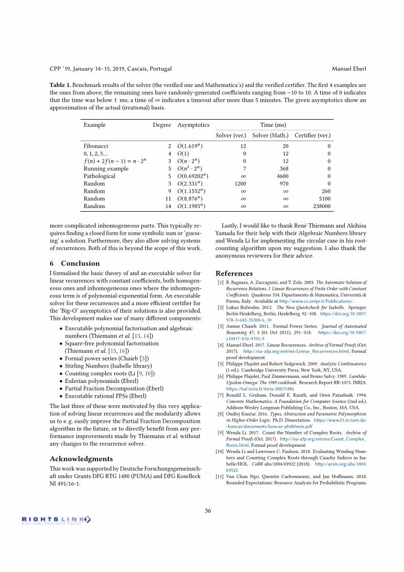
CPP ’19, January 14–15, 2019, Cascais, Portugal Manuel Eberl
Table 1. Benchmark results of the solver (the verified one and Mathematica’s) and the verified certifier. The first 4 examples arethe ones from above; the remaining ones have randomly-generated coefficients ranging from −10 to 10. A time of 0 indicatesthat the time was below 1 ms; a time of ∞ indicates a timeout after more than 5 minutes. The given asymptotics show anapproximation of the actual (irrational) basis.
Example Degree Asymptotics Time (ms)Solver (ver.) Solver (Math.) Certifier (ver.)
Fibonacci 2 O(1.619n) 12 20 00, 1, 2, 3... 4 O(1) 0 12 0f (n) + 2f (n − 1) = n · 2n 3 O(n · 2n) 0 12 0Running example 5 O(n2 · 2n) 7 368 0Pathological 5 O(0.69202n) ∞ 4600 0Random 3 O(2.331n) 1200 970 0Random 9 O(1.1552n) ∞ ∞ 260Random 11 O(8.876n) ∞ ∞ 5100Random 14 O(1.1985n) ∞ ∞ 238000
more complicated inhomogeneous parts. This typically re-quires finding a closed form for some symbolic sum or ‘guess-ing’ a solution. Furthermore, they also allow solving systemsof recurrences. Both of this is beyond the scope of this work.
6 ConclusionI formalised the basic theory of and an executable solver forlinear recurrences with constant coefficients, both homogen-eous ones and inhomogeneous ones where the inhomogen-eous term is of polynomial-exponential form. An executablesolver for these recurrences and a more efficient certifier forthe ‘Big-O’ asymptotics of their solutions is also provided.This development makes use of many different components:• Executable polynomial factorisation and algebraicnumbers (Thiemann et al. [13, 14])• Square-free polynomial factorisation(Thiemann et al. [15, 16])• Formal power series (Chaieb [3])• Stirling Numbers (Isabelle library)• Counting complex roots (Li [9, 10])• Eulerian polynomials (Eberl)• Partial Fraction Decomposition (Eberl)• Executable rational FPSs (Eberl)
The last three of these were motivated by this very applica-tion of solving linear recurrences and the modularity allowsus to e. g. easily improve the Partial Fraction Decompositionalgorithm in the future, or to directly benefit from any per-formance improvements made by Thiemann et al. withoutany changes to the recurrence solver.
AcknowledgmentsThisworkwas supported byDeutsche Forschungsgemeinsch-aft under Grants DFG RTG 1480 (PUMA) and DFG KoselleckNI 491/16-1.
Lastly, I would like to thank René Thiemann and AkihisaYamada for their help with their Algebraic Numbers libraryand Wenda Li for implementing the circular case in his root-counting algorithm upon my suggestion. I also thank theanonymous reviewers for their advice.
References[1] R. Bagnara, A. Zaccagnini, and T. Zolo. 2003. The Automatic Solution of
Recurrence Relations. I. Linear Recurrences of Finite Order with ConstantCoefficients. Quaderno 334. Dipartimento di Matematica, Università diParma, Italy. Available at http://www.cs.unipr.it/Publications/.
[2] Lukas Bulwahn. 2012. The New Quickcheck for Isabelle. SpringerBerlin Heidelberg, Berlin, Heidelberg, 92–108. https://doi.org/10.1007/978-3-642-35308-6_10
[3] Amine Chaieb. 2011. Formal Power Series. Journal of AutomatedReasoning 47, 3 (01 Oct 2011), 291–318. https://doi.org/10.1007/s10817-010-9195-9
[4] Manuel Eberl. 2017. Linear Recurrences. Archive of Formal Proofs (Oct.2017). http://isa-afp.org/entries/Linear_Recurrences.html, Formalproof development.
[5] Philippe Flajolet and Robert Sedgewick. 2009. Analytic Combinatorics(1 ed.). Cambridge University Press, New York, NY, USA.
[6] Philippe Flajolet, Paul Zimmermann, and Bruno Salvy. 1989. Lambda-Upsilon-Omega: The 1989 cookbook. Research Report RR-1073. INRIA.https://hal.inria.fr/inria-00075486
[7] Ronald L. Graham, Donald E. Knuth, and Oren Patashnik. 1994.Concrete Mathematics: A Foundation for Computer Science (2nd ed.).Addison-Wesley Longman Publishing Co., Inc., Boston, MA, USA.
[8] Ondřej Kunčar. 2016. Types, Abstraction and Parametric Polymorphismin Higher-Order Logic. Ph.D. Dissertation. https://www21.in.tum.de/~kuncar/documents/kuncar-phdthesis.pdf
[9] Wenda Li. 2017. Count the Number of Complex Roots. Archive ofFormal Proofs (Oct. 2017). http://isa-afp.org/entries/Count_Complex_Roots.html, Formal proof development.
[10] Wenda Li and Lawrence C. Paulson. 2018. Evaluating Winding Num-bers and Counting Complex Roots through Cauchy Indices in Isa-belle/HOL. CoRR abs/1804.03922 (2018). http://arxiv.org/abs/1804.03922
[11] Van Chan Ngo, Quentin Carbonneaux, and Jan Hoffmann. 2018.Bounded Expectations: Resource Analysis for Probabilistic Programs.
36
Verified Solving and Asymptotics of Linear Recurrences CPP ’19, January 14–15, 2019, Cascais, Portugal
In Proceedings of the 39th ACM SIGPLAN Conference on ProgrammingLanguage Design and Implementation (PLDI 2018). ACM, New York,NY, USA, 496–512. https://doi.org/10.1145/3192366.3192394
[12] Joël Ouaknine and James Worrell. 2015. On Linear Recurrence Se-quences and Loop Termination. ACM SIGLOG News 2, 2 (April 2015),4–13. https://doi.org/10.1145/2766189.2766191
[13] René Thiemann and Akihisa Yamada. 2015. Algebraic Numbers inIsabelle/HOL. Archive of Formal Proofs (Dec. 2015). http://isa-afp.org/entries/Algebraic_Numbers.html Formal proof development.
[14] René Thiemann and Akihisa Yamada. 2016. Algebraic numbers inIsabelle/HOL. Springer International Publishing, Cham, 391–408. https:
//doi.org/10.1007/978-3-319-43144-4_24[15] René Thiemann and Akihisa Yamada. 2016. Formalizing Jordan Nor-
mal Forms in Isabelle/HOL. In Proceedings of the 5th ACM SIGPLANConference on Certified Programs and Proofs (CPP 2016). ACM, NewYork, NY, USA, 88–99. https://doi.org/10.1145/2854065.2854073
[16] René Thiemann and Akihisa Yamada. 2016. Polynomial Factoriza-tion. Archive of Formal Proofs (Jan. 2016). http://isa-afp.org/entries/Polynomial_Factorization.html, Formal proof development.
[17] Bohua Zhan and Maximilian P. L. Haslbeck. 2018. Verifying Asymp-totic Time Complexity of Imperative Programs in Isabelle. CoRRabs/1802.01336 (2018). http://arxiv.org/abs/1802.01336
37