HAL Id: hal-00146246https://hal.archives-ouvertes.fr/hal-00146246

Preprint submitted on 14 May 2007

HAL is a multi-disciplinary open accessarchive for the deposit and dissemination of sci-entific research documents, whether they are pub-lished or not. The documents may come fromteaching and research institutions in France orabroad, or from public or private research centers.

L’archive ouverte pluridisciplinaire HAL, estdestinée au dépôt et à la diffusion de documentsscientifiques de niveau recherche, publiés ou non,émanant des établissements d’enseignement et derecherche français ou étrangers, des laboratoirespublics ou privés.

Linear Prediction of Long-Memory Processes:Asymptotic Results on Mean-squared Errors

Fanny Godet

To cite this version:Fanny Godet. Linear Prediction of Long-Memory Processes: Asymptotic Results on Mean-squaredErrors. 2007. hal-00146246

hal-

0014

6246

, ver

sion

1 -

14

May

200

7

Linear Prediction of Long-Memory Processes:

Asymptotic Results on Mean-squared Errors

Fanny Godet∗

Laboratoire de Mathematiques Jean Leray, UMR CNRS 6629Universite de Nantes 2 rue de la Houssiniere - BP 92208 F-44322 Nantes Cedex 3

14th May 2007

Abstract

We present two approaches for linear prediction of long-memory time series. The first ap-proach consists in truncating the Wiener-Kolmogorov predictor by restricting the observationsto the last k terms, which are the only available values in practice. We derive the asymptoticbehaviour of the mean-squared error as k tends to +∞. By contrast, the second approach isnon-parametric. An AR(k) model is fitted to the long-memory time series and we study theerror that arises in this misspecified model.

Keywords: long-memory, linear model, autoregressive process, forecast errorARMA (autoregressive moving-average) processes are often called short-memory processes be-

cause their covariances decay rapidly (i.e. exponentially). On the other hand, a long-memory processis characterised by the following feature: the autocovariance function σ decays more slowly i.e. it isnot absolutely summable. They are so-named because of the strong association between observa-tions widely separated in time. The long-memory time series models have attracted much attentionlately and there is now a growing realisation that time series possessing long-memory characteristicsarise in subject areas as diverse as Economics, Geophysics, Hydrology or telecom traffic (see, e.g.,[Mandelbrot and Wallis, 1969] and [Granger and Joyeux, 1980]). Although there exists substantialliterature on the prediction of short-memory processes(see [Bhansali, 1978] for the univariate caseor [Lewis and Reinsel, 1985] for the multivariate case), there are fewer results for long-memory timeseries. In this paper, we consider the question of the prediction of the latter.

More precisely, we compare two prediction methods for long-memory process. Our goal is a linearpredictor of Xk+h based on observed time points which is optimal in the sense that it minimizes themean-squared error. The paper is organized as follows. First we introduce our model and our mainassumptions. Then, in section 2, we study the best linear predictor i.e. the Wiener-Kolmogorovpredictor proposed by [Whittle, 1963] and by [Bhansali and Kokoszka, 2001] for long-memory timeseries. In practice, only the last k values of the process are available. Therefore we need to truncatethe infinite series in the definition of the predictor and to derive the asymptotic behaviour of themean-squared error as k tends to +∞.

∗fanny.godet@math.univ-nantes.fr

I would like to thank Anne Philippe, my PhD advisor, who monitored my work.

1

In Section 3 we discuss the asymptotic properties of the forecast error if we fit a misspecifiedAR(k) model to a long-memory time series. This approach has been proposed by [Ray, 1993] forfractional noise series F(d). His simulations show that high-order AR-models predict fractionalintegrated noise very well.

Finally in Section 4 we compare the two previous methods for h-step prediction. We give someasymptotic properties of the mean-squared error of the linear least-squares predictor as h tends to+∞ in the particular case of long-memory processes. Then we study our k-th order predictors orderas k tends to +∞.

1 Model

Let (Xn)n∈Z be a discrete-time (weakly) stationary process in L2 with mean 0 and σ its autocovari-ance function. We assume that the process (Xn)n∈Z is a long-memory process i.e.:

∞∑

k=−∞

|σ(k)| = ∞.

The process (Xn)n∈Z admits an infinite moving average representation as follows:

Xn =

∞∑

j=0

bjεn−j (1)

where (εn)n∈Z is a white-noise series consisting of uncorrelated random variables, each with meanzero and variance σ2

ε and (bj)j∈N are square-summable. We shall further assume that (Xn)n∈Z

admits an infinite autoregressive representation:

εn =∞∑

j=0

ajXn−j , (2)

where the (aj)j∈N are absolutely summable. We assume also that (aj)j∈N and (bj)j∈N, occurringrespectively in (2) and (1), satisfy the following conditions for all δ > 0:

|aj | ≤ C1j−d−1+δ (3)

|bj| ≤ C2jd−1+δ . (4)

where C1 and C2 are constants and d is a parameter verifying d ∈]0, 1/2[. For example, a FARIMAprocess (Xn)n∈Z is the stationary solution to the difference equations:

φ(B)(1 − B)dXn = θ(B)εn

where (εn)n∈Z is a white noise series, B is the backward shift operator and φ and θ are polynomialswith no zeroes on the unit disk. Its coefficients verify

|aj | ∼+∞

C1j−d−1

|bj | ∼+∞

C2jd−1

2

and thus (3) and (4) hold. When φ = θ = 1, the process (Xn)n∈Z is called fractionally integratednoise and denoted F(d). More generally, (aj)j∈N and (bj)j∈N verify conditions (3) and (4) if:

|aj | ∼+∞

L(j)j−d−1

|bj | ∼+∞

L′(j)jd−1

where L and L′ are slowly varying functions. A positive function L is a slowly varying functionin the sense of [Zygmund, 1968] if, for any δ > 0, x 7→ x−δL(x) is decreasing and x 7→ xδL(x) isincreasing.

The condition (4) implies that the autocovariance function σ of the process (Xn)n∈Z verifies:

∀δ > 0,∃C3 ∈ R, |σ(j)| ≤ C3j2d−1+δ . (5)

Notice that it suffices to prove (5) for δ near 0 in order to verify (5) for δ > 0 arbitrarily chosen.So we prove (5) for δ < 1−2d

2 :

σ(k) =

+∞∑

j=0

bjbj+k

|σ(k)| ≤

+∞∑

j=1

|bjbj+k| + |b0bk|

≤ C22

+∞∑

j=1

jd−1+δ(k + j)d−1+δ + |b0bk|

≤ C22

∫ +∞

0jd−1+δ(k + j)d−1+δdj + |b0bk|

≤ C22k2d−1+2δ

∫ +∞

0jd−1+δ(1 + j)d−1+δdj + C2k

d−1+δ

≤ C3k2d−1+2δ

More accurately, [Inoue, 1997] has proved than if:

bj ∼ L (j) jd−1

thenσ(j) ∼ j2d−1 [L (j)]2 β(1 − 2d, d)

where L is a slowly varying function and β is the beta function. The converse is not true, wemust have more assumptions about the series (bj)j∈N in order to get an asymptotic equivalent for(σ(j))j∈N (see [Inoue, 2000]).

2 Wiener-Kolmogorov Next Step Prediction Theory

2.1 Wiener-Kolmogorov Predictor

The aim of this part is to compute the best linear one-step predictor (with minimum mean-squaredistance from the true random variable) knowing all the past Xk+1−j , j 6 1. Our predictor is

3

therefore an infinite linear combination of the infinite past:

Xk(1) =

∞∑

j=0

λ(j)Xk−j

where (λ(j))j∈N are chosen to ensure that the mean squared prediction error:

E[(

Xk(1) − Xk+1

)2]

is as small as possible. Following [Whittle, 1963], and in view of the moving average representation

of (Xn)n∈Z, we may rewrite our predictor Xk(1) as:

Xk(1) =∞∑

j=0

φ(j)εk−j .

where (φ(j))j∈N depends only on (λ(j))j∈N and (ǫn)n∈Z and (aj)j∈N are defined in (2). From theinfinite moving average representation of (Xn)n∈Z given below in (1), we can rewrite the mean-squared prediction error as:

E[(

Xk(1) − Xk+1

)2]= E

∞∑

j=0

φ(j)εk−j −∞∑

j=0

b(j)εk+1−j

2

= E

εk+1 −

∞∑

j=0

(φ(j) − b(j + 1)) εk−j

2

=

1 +

∞∑

j=0

(bj+1 − φ(j)

)2σ2

ε

since the random variables (εn)n∈Z are uncorrelated with variance σ2ε . The smallest mean-squared

prediction error is obtained when setting φ(j) = bj+1 for j ≥ 0.The smallest prediction error of (Xn)n∈Z is σ2

ε within the class of linear predictors. Furthermore,if

A(z) =

+∞∑

j=0

ajzj,

denotes the characteristic polynomial of the (a(j))j∈Z and

B(z) =+∞∑

j=0

bjzj ,

that of the (a(j))j∈Z, then in view of the identity, A(z) = B(z)−1, |z| ≤ 1, we may write:

Xk(1) = −

∞∑

j=1

ajXk+1−j. (6)

4

2.2 Mean Squared Prediction Error when the Predictor is Truncated

In practice, we only know a finite subset of the past, the one which we have observed. So thepredictor should only depend on the observations. Assume that we only know the set X1, . . . ,Xkand that we replace the unknown values by 0, then we have the following new predictor:

X ′k(1) = −

k∑

j=1

ajXk+1−j. (7)

It is equivalent to say that we have truncated the infinite series (6) to k terms. The followingproposition provides us the asymptotic properties of the mean squared prediction error as a functionof k.

Proposition 2.2.1. Let (Xn)n∈Z be a linear stationary process defined by (1), (2) and verifying

conditions (3) and (4). We can approximate the mean-squared prediction error of X ′k(1) by:

∀δ > 0, E([

Xk+1 − X ′k(1)

]2)= σ2

ε + O(k−1+δ).

Furthermore, this rate of convergence O(k−1) is optimal since for fractionally integrated noise, wehave the following asymptotic equivalent:

E([

Xk+1 − X ′k(1)

]2)= σ2

ε + Ck−1 + o(k−1

).

Note that the prediction error is the sum of σ2ε , the error of Wiener-Kolmogorov model and the

error due to the truncation to k terms which is bounded by O(k−1+δ) for all δ > 0.

Proof.

Xk+1 − X ′k(1) = Xk+1 − Xk(1) + Xk(1) − X ′

k(1)

= Xk+1 −+∞∑

j=0

bj+1εk−j −+∞∑

j=k+1

ajXk+1−j

= εk+1 −

+∞∑

j=k+1

ajXk+1−j . (8)

The two parts of the sum (8) are orthogonal for the inner product associated with the mean squarenorm. Consequently:

E([

Xk+1 − X ′k(1)

]2)= σ2

ε +

∞∑

j=k+1

∞∑

l=k+1

ajalσ(l − j).

For the second term of the sum we have:∣∣∣∣

+∞∑

j=k+1

+∞∑

l=k+1

ajalσ(l − j)

∣∣∣∣ =

∣∣∣∣2+∞∑

j=k+1

aj

+∞∑

l=j+1

alσ(l − j) +

+∞∑

j=k+1

a2jσ(0)

∣∣∣∣

≤ 2+∞∑

j=k+1

|aj | |aj+1| |σ(1)| ++∞∑

j=k+1

a2jσ(0)

+2

+∞∑

j=k+1

|aj |

+∞∑

l=j+2

|al||σ(l − j)|

5

from the triangle inequality, it follows that:

∣∣∣∣+∞∑

j=k+1

+∞∑

l=k+1

ajalσ(l − j)

∣∣∣∣

≤ C21C3

2

+∞∑

j=k+1

j−d−1+δ(j + 1)−d−1+δ +

+∞∑

j=k+1

(j−d−1+δ

)2

(9)

+ 2C21C3

+∞∑

j=k+1

j−d−1+δ+∞∑

l=j+2

l−d−1+δ|l − j|2d−1+δ (10)

for all δ > 0 from inequalities (3) and (5). Assume now that δ < 1/2 − d. For the terms (9),since j 7→ j−d−1+δ(j + 1)−d−1+δ is a positive and decreasing function on R

+, we have the followingapproximations:

2C21C3

+∞∑

j=k+1

j−d−1+δ(j + 1)−d−1+δ ∼ 2C21C3

∫ +∞

kj−d−1+δ(j + 1)−d−1+δdj

∼2C2

1C3

1 + 2d − 2δk−2d−1+2δ

Since the function j 7→(j−d−1+δ

)2is also positive and decreasing, we can establish in a similar way

that:

C21C3

+∞∑

j=k+1

(j−d−1+δ

)2∼ C2

1C3

∫ +∞

k

(j−d−1+δ

)2dj

∼C2

1C3

1 + 2d − 2δk−2d−1+2δ.

For the infinite double series (10), we will similarly compare the series with an integral. In thenext Lemma, we establish the necessary result for this comparison:

Lemma 2.2.1. Let g the function (l, j) 7→ j−d−1+δ l−d−1+δ |l − j|2d−1+δ . Let m and n be two

positive integers. We assume that δ < 1 − 2d and m ≥ δ−d−1δ+2d−1 for all δ ∈

]0, δ−d−1

δ+2d−1

[. We will call

An,m the square [n, n + 1] × [m,m + 1]. If n ≥ m + 1 then∫

An,m

g(l, j) dj dl ≥ g(n + 1,m).

Assume now that δ < 1− 2d without loss of generality. Thanks to the previous Lemma and theasymptotic equivalents of (9), there exists K ∈ N such that if k > K:

∣∣∣∣+∞∑

j=k+1

+∞∑

l=k+1

ajalσ(l − j)

∣∣∣∣ ≤ C

∫ +∞

k+1j−d−1+δ

[∫ +∞

jl−d−1+δ(l − j)2d−1+δdl

]dj + O

(k−2d−1+2δ

)

By using the substitution jl′ = l in the integral over l we obtain:

∣∣∣∣+∞∑

j=k+1

+∞∑

l=k+1

ajalσ(l − j)

∣∣∣∣ ≤ C ′

∫ +∞

k+1j−2+3δ

∫ +∞

1l−d−1+δ(l − 1)2d−1+δdldj + O

(k−2d−1

).

6

Since if δ < (1 − d)/2 ∫ +∞

1l−d−1+δ(l − 1)2d−1+δdl < +∞,

it follows:

∣∣∣∣+∞∑

j=k+1

+∞∑

l=k+1

ajalσ(l − j)

∣∣∣∣ ≤ O(k−1+3δ

)+ O

(k−2d−1

)

≤ O(k−1+3δ

). (11)

If δ > 0, δ < 1 − 2d and δ < (1 − d)/2, we have:

∣∣∣∣+∞∑

j=k+1

+∞∑

l=k+1

ajalσ(l − j)

∣∣∣∣ = O(k−1+3δ

).

Notice that if the equality is true under the assumptions δ > 0, δ < 1 − 2d and δ < (1 − d)/2, it isalso true for any δ > 0. Therefore we have proven the first part of the theorem.We prove now that there exists long-memory processes whose prediction error attains the rate ofconvergence k−1. Assume now that (Xn)n∈Z is fractionally integrated noise F(d), which is thestationary solution of the difference equation:

Xn = (1 − B)−dεn (12)

with B the usual backward shift operator, (εn)n∈Z is a white-noise series and d ∈ ]0, 1/2[ (see forexample [Brockwell and Davis, 1991]). We can compute the coefficients and obtain that:

∀j > 0, aj =Γ(j − d)

Γ(j + 1)Γ(−d)and ∀j ≥ 0, σ(j) =

(−1)jΓ(1 − 2d)

Γ(j − d + 1)Γ(1 − j − d)σ2

ε

then we have:∀j > 0, aj < 0 and ∀j ≥ 0, σ(j) > 0

and

aj ∼j−d−1

Γ(−d)and σ(j) ∼

j2d−1Γ(1 − 2d)

Γ(d)Γ(1 − d)when j → ∞.

In this particular case, we can estimate the prediction error more precisely:

+∞∑

k+1

+∞∑

k+1

ajalσ(l − j) =

+∞∑

k+1

|aj|

+∞∑

j+1

|al||σ(l − j)| +

+∞∑

k+1

a2jσ(0)

∼Γ(1 − 2d)

Γ(−d)2Γ(d)Γ(1 − d)

∫ +∞

k+1j−2

∫ +∞

1/j+1l−d−1(l − 1)2d−1dldj + O

(k−2d−1

)

+∞∑

k+1

+∞∑

k+1

ajalσ(l − j) ∼Γ(1 − 2d)Γ(2d)

Γ(−d)2Γ(d)Γ(1 + d)k−1 (13)

The asymptotic bound O(k−1) is therefore as small as possible.

7

In the specific case of fractionally integrated noise, we may write the prediction error as:

E([

Xk+1 − X ′k(1)

]2)= σ2

ε + C(d)k−1 + o(k−1

)

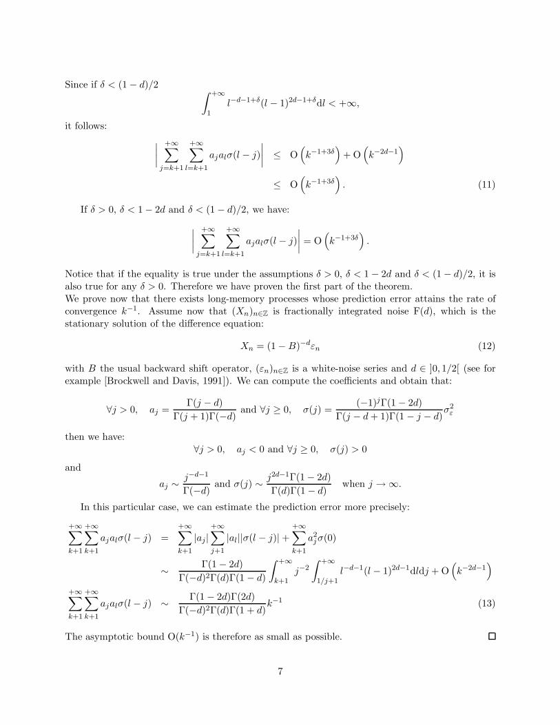
and we can express C(d) as a function of d:

C(d) =Γ(1 − 2d)Γ(2d)

Γ(−d)2Γ(d)Γ(1 + d). (14)

It is easy to prove that C(d) → +∞ as d → 1/2 and we may write the following asymptoticequivalent as d → 1/2:

C(d) ∼1

(1 − 2d)Γ(−1/2)2Γ(1/2)Γ(3/2). (15)

As d → 0, C(d) → 0 and we have the following equivalent as d → 0:

C(d) ∼ d2.

Figure 2.1: Behaviour of constant C(d), d ∈ [0, 1/2[, defined in (14)

0.0 0.1 0.2 0.3 0.4

0.0

0.1

0.2

0.3

0.4

d

C(d

)

As the figure 2.1 suggests and the asymptotic equivalent given in (15) proves, the mean-squarederror tends to +∞ as d → 1/2. By contrast, the constant C(d) takes small values for d in a largeinterval of [0, 1/2[. Although the rate of convergence has a constant order k−1, the forecast erroris bigger when d → 1/2. This result is not surprising since the correlation between the randomvariable, which we want to predict, and the random variables, which we take equal to 0, increaseswhen d → 1/2.

8

Truncating to k terms the series which defines the Wiener-Kolmogorov predictor amounts to usingan AR(k) model for predicting. Therefore in the following section we look for the AR(k) whichminimizes the forecast error.

3 The Autoregressive Models Fitting Approach

In this section we develop a generalisation of the “autoregressive model fitting” approach developedby [Ray, 1993] in the case of fractionally integrated noise F(d) (defined in (12)). We study theasymptotic properties of the forecast mean-squared error when we fit a misspecified AR(k) modelto the long-memory time series (Xn)n∈Z.

3.1 Rationale

Let Φ a kth degree polynomial defined by:

Φ(z) = 1 − a1,kz − . . . − ak,kzk.

We assume that Φ has no zeroes on the unit disk. We define the process (ηn)n∈Z by:

∀n ∈ Z, ηn = Φ(B)Xn

where B is the backward shift operator. Note that (ηn)n∈Z is not a white noise series because(Xn)n∈Z is a long-memory process and hence does not belong to the class of autoregressive processes.Since Φ has no root on the unit disk, (Xn)n∈Z admits a moving-average representation as the fittedAR(k) model in terms of (ηn)n∈Z:

Xn =

∞∑

j=0

c(j)ηn−j .

If (Xn)n∈Z was an AR(k) associated with the polynomial Φ, the best next step linear predictorwould be:

Xn(1) =∞∑

j=1

c(i)ηt+1−i

= a1,kXn + . . . + ak,kXn+1−k si n > k.

Here (Xn)n∈Z is a long-memory process which verifies the assumptions of Section 1. Our goal is toderive a closed formula for the polynomial Φ which minimizes the forecast error and to estimatethis error.

3.2 Mean-Squared Error

There exists two approaches in order to define the coefficients of the kth degree polynomial Φ: thespectral approach and the time approach.

In the time approach, we choose to define the predictor as the projection mapping on to theclosed span of the subset Xn, . . . ,Xn+1−k of the Hilbert space L2(Ω,F , P) with inner product

9

< X,Y >= E(XY ). Consequently the coefficients of Φ verify the equations, which are called thekth order Yule-Walker equations:

∀j ∈ J1, kK,

k∑

i=1

ai,kσ(i − j) = σ(j) (16)

The mean-squared prediction error is:

E[(

Xn(1) − Xn+1

)2]= c(0)2E(η2

n+1) = E(η2n+1).

We may write the moving average representation of (ηn)n∈N in terms of (εn)n∈N:

ηn =

∞∑

j=0

min(j,p)∑

k=0

Φkb(j − k)εn−j

=∞∑

j=0

t(j)εn−j

with

∀j ∈ N, t(j) =

min(j,p)∑

k=0

Φkb(j − k).

Finally we obtain:

E[(

Xn(1) − Xn+1

)2]=

∞∑

j=0

t(j)2σ2ε .

In the spectral approach, minimizing the prediction error is equivalent to minimizing a contrastbetween two spectral densities: ∫ π

−π

f(λ)

g(λ,Φ)dλ

where f is the spectral density of Xn and g(.,Φ) is the spectral density of the AR(p) process definedby the polynomial Φ (see for example [Yajima, 1993]),so:

∫ π

−π

f(λ)

g(λ,Φ)dλ =

∫ π

−π

∣∣∣∞∑

j=0

b(j)e−ijλ∣∣∣2∣∣∣Φ(e−iλ)

∣∣∣2dλ

=

∫ π

−π|

∞∑

j=0

t(j)e−ijλ|2dλ

= 2π∞∑

j=0

t(j)2.

In both approaches we need to minimize∑∞

j=0 t(j).

10

3.3 Rate of Convergence of the Error by AR(k) Model Fitting

In the next theorem we derive an asymptotic expression for the prediction error by fitting autore-gressive models to the series:

Theorem 3.3.1. Assume that (Xn)n∈Z is a long-memory process which verifies the assumptions ofSection 1. If 0 < d < 1

2 :

E[(

Xk(1) − Xk+1

)2]− σ2

ε = O(k−1)

Proof. Since fitting an AR(k) model minimizes the forecast error using k observations, the error byusing truncation is bigger. Since the truncation method involves an error bounded by O

(k−1

), we

obtain:E[(

Xk(1) − Xk+1

)2]− σ2

ε = O(k−1).

Consequently we only need to prove that this rate of convergence is attained . This is the casefor the fractionally integrated processes defined in (12). We want the error made when fitting anAR(k) model in terms of the Wiener-Kolmogorov truncation error. Note first that the variance ofthe white noise series is equal to:

σ2ε =

∫ π

−πf(λ)

∣∣∣∣∣∣

+∞∑

j=0

ajeijλ

∣∣∣∣∣∣

2

dλ.

Therefore in the case of a fractionally integrated process F(d) we need only show that:

∫ π

−πf(λ)

∣∣∣∣∣∣

+∞∑

j=0

ajeijλ

∣∣∣∣∣∣

2

dλ −σ2

ε

2π

∫ π

−π

f(λ)

g(λ,Φk)dλ ∼ C(k−1).

∫ π

−πf(λ)

∣∣∣∣∣∣

+∞∑

j=0

ajeijλ

∣∣∣∣∣∣

2

dλ −σ2

ε

2π

∫ π

−π

f(λ)

g(λ,Φk)dλ =

∫ π

−πf(λ)

∣∣∣∣∣∣

+∞∑

j=0

ajeijλ

∣∣∣∣∣∣

2

−

∣∣∣∣∣∣

k∑

j=0

aj,keijλ

∣∣∣∣∣∣

2 dλ

=+∞∑

j=0

+∞∑

l=0

(ajal − aj,kal,k) σ(j − l)

we set aj,k = 0 if j > k.

+∞∑

j=0

+∞∑

l=0

(ajal − aj,kal,k) σ(j − l) (17)

=+∞∑

j=0

+∞∑

l=0

(ajal − aj,kal)σ(j − l) ++∞∑

j=0

+∞∑

l=0

(aj,kal − aj,kal,k)σ(j − l)

=

+∞∑

j=0

(aj − aj,k)

+∞∑

l=0

alσ(l − j) +

k∑

j=0

aj,k

+∞∑

l=0

(al − al,k)σ(j − l) (18)

11

We first study the first term of the sum (18). For any j > 0 , we have∑+∞

l=0 alσ(l − j) = 0:

εn =

∞∑

j=0

alXn−l

Xn−jεn =∞∑

l=0

alXn−lXn−j

E (Xn−jεn) =∞∑

l=0

alσ(l − j)

E

(∞∑

l=0

blεn−j−lεn

)=

∞∑

l=0

alσ(l − j)

and we conclude that∑+∞

l=0 alσ(l − j) = 0 because (εn)n∈Z is an uncorrelated white noise. We canthus rewrite the first term of (18) like:

+∞∑

j=0

(aj − aj,k)

+∞∑

l=0

alσ(l − j) = (a0 − a0,k)

+∞∑

l=0

alσ(l)

= 0

since a0 = a0,k = 1 according to definition. Next we study the second term of the sum (18):

k∑

j=0

aj,k

+∞∑

l=0

(al − al,k)σ(j − l).

And we obtain that:

k∑

j=0

aj,k

+∞∑

l=0

(al − al,k)σ(j − l) =

k∑

j=1

(aj,k − aj)

k∑

l=1

(al − al,k)σ(j − l)

+

k∑

j=1

(aj,k − aj)

+∞∑

l=k+1

alσ(j − l) (19)

+

k∑

j=0

aj

k∑

l=1

(al − al,k)σ(j − l) (20)

+

k∑

j=0

aj

+∞∑

l=k+1

alσ(j − l)

Similarly we rewrite the term (19) using the Yule-Walker equations:

k∑

j=1

(aj,k − aj)+∞∑

l=k+1

alσ(j − l) = −k∑

j=1

(aj,k − aj)k∑

l=0

alσ(j − l)

12

We then remark that this is equal to (20). Hence it follows that:

k∑

j=0

aj,k

+∞∑

l=0

(al − al,k)σ(j − l) =k∑

j=1

(aj,k − aj)k∑

l=1

(al − al,k)σ(j − l)

+2k∑

j=1

(aj,k − aj)+∞∑

l=k+1

alσ(j − l)

+k∑

j=0

aj

+∞∑

l=k+1

alσ(j − l) (21)

On a similar way we can rewrite the third term of the sum (21) using Fubini Theorem:

k∑

j=0

aj

+∞∑

l=k+1

alσ(j − l) = −

+∞∑

j=k+1

+∞∑

l=k+1

ajalσ(j − l).

This third term is therefore equal to the forecast error in the method of prediction by truncation.In order to compare the prediction error by truncating the Wiener-Kolmogorov predictor and

by fitting an autoregressive model to a fractionally integrated process F(d), we need the sign of allthe components of the sum (21). For a fractionally integrated noise, we know the explicit formulafor aj and σ(j):

∀j > 0, aj =Γ(j − d)

Γ(j + 1)Γ(−d)< 0 and ∀j ≥ 0, σ(j) =

(−1)jΓ(1 − 2d)

Γ(j − d + 1)Γ(1 − j − d)σ2

ε > 0.

In order to get the sign of aj,k −aj we use the explicit formula given in [Brockwell and Davis, 1988]and we easily obtain that aj,k − aj is negative for all j ∈ J1, kK.

aj − aj,k =Γ(j − d)

Γ(j + 1)Γ(−d)−

Γ(k + 1)Γ(j − d)Γ(k − d − j + 1)

Γ(k − j + 1)Γ(j + 1)Γ(−d)Γ(k − d + 1)

= −aj

(−1 +

Γ(k + 1)Γ(k − d − j + 1)

Γ(k − j + 1)Γ(k − d + 1)

)

= −aj

(k...(k − j + 1)

(k − d)...(k − d − j + 1)− 1

)

> 0

since ∀j ∈ N∗ aj < 0. To give an asymptotic equivalent for the prediction error, we use the sum

given in (21). We have the sign of the three terms: the first is negative, the second is positiveand the last is negative. Moreover the third is equal to the forecast error by truncation and wehave proved that this asymptotic equivalent has order O(k−1). The prediction error by fitting anautoregressive model converges faster to 0 than the error by truncation only if the second term isequivalent to Ck−1, with C constant. Consequently, we search for a bound for aj − aj,k given the

13

explicit formula for these coefficients (see for example [Brockwell and Davis, 1988]):

aj − aj,k =Γ(j − d)

Γ(j + 1)Γ(−d)−

Γ(k + 1)Γ(j − d)Γ(k − d − j + 1)

Γ(k − j + 1)Γ(j + 1)Γ(−d)Γ(k − d + 1)

= −aj

(−1 +

Γ(k + 1)Γ(k − d − j + 1)

Γ(k − j + 1)Γ(k − d + 1)

)

= −aj

(k...(k − j + 1)

(k − d)...(k − d − j + 1)− 1

)

= −aj

(j−1∏

m=0

(1 − l

k

1 − l+dk

)− 1

)

= −aj

(j−1∏

m=0

(1 +

dk

1 − d+lk

)− 1

).

Then we use the following inequality:

∀x ∈ R, 1 + x ≤ exp(x)

which gives us:

aj − aj,k ≤ −aj

(exp

(j−1∑

m=0

dk

1 − d+lk

)− 1

)

≤ −aj

(exp

(d

j−1∑

m=0

1

k − d − l

)− 1

)

≤ −aj exp

(d

j−1∑

m=0

1

k − d − l

)

According to the previous inequality, we have:

k∑

j=1

(aj − aj,k)

+∞∑

l=k+1

−alσ(j − l) =

k−1∑

j=1

(aj − aj,k)

+∞∑

l=k+1

−alσ(j − l)

+(ak − ak,k)+∞∑

l=k+1

−alσ(k − l)

≤

k−1∑

j=1

−aj exp

(d

j−1∑

m=0

1

k − d − m

)+∞∑

l=k+1

−alσ(j − l)

+(−ak) exp

(d

k−1∑

m=0

1

k − d − m

)+∞∑

l=k+1

−alσ(k − l)

≤

k−1∑

j=1

−aj exp

(d

∫ j

0

1

k − d − mdm

) +∞∑

l=k+1

−alσ(j − l)

+(−ak)k3

2d

+∞∑

l=k+1

−alσ(k − l)

14

As the function x 7→ 1k−d−x is increasing, we use the Integral Test Theorem. The inequality on the

second term follows from:

k−1∑

m=0

1

k − d − m∼ ln(k)

≤3

2ln(k)

for k large enough. Therefore there exists K such that for all k ≥ K:

k∑

j=1

(aj − aj,k)+∞∑

l=k+1

−alσ(j − l) ≤k−1∑

j=1

−aj exp

(d ln

(k − d

k − d − j

)) +∞∑

l=k+1

−alσ(j − l)

+(−ak)k3

2d

+∞∑

l=k+1

−alσ(0)

≤ C(k − d)dk−1∑

j=1

j−d−1(k − d − j)−d+∞∑

l=k+1

l−d−1(l − j)2d−1

+Ck−d−1k3

2dk−d

≤C

(k − d)2

∫ 1

1/(k−d)j−d−1(1 − j)−d

∫ +∞

1l−d−1(l − 1)2d−1dldj

+Ck− 1

2d−1

≤ C ′(k − d)−2+d + Ck− 1

2d−1

and so the positive term has a smaller asymptotic order than the forecast error made by truncating.Therefore we have proved that in the particular case of F(d) processes, the two prediction errorsare equivalent to Ck−1 with C constant.

The two approaches to next-step prediction, by truncation to k terms or by fitting an autoregres-sive model AR(k) have consequently a prediction error with the same rate of convergence k−1. Soit is interesting to study how the second approach improves the prediction. The following quotient:

r(k) :=

∑kj=1(aj,k − aj)

∑kl=1(al − al,k)σ(j − l) + 2

∑kj=1(aj,k − aj)

∑+∞l=k+1 alσ(j − l)

∑kj=0 aj

∑+∞l=k+1 alσ(j − l)

(22)

is the ratio of the difference between the two prediction errors and the prediction error by truncatingin the particular case of a fractionally integrated noise F(d). The figure 3.1 shows that the predictionby truncation incurs a larger performance loss when d → 1/2. The improvement reaches 50 percent when d > 0.3 and k > 20.

After obtaining asymptotic equivalent for next step predictor, we will generalize the two methodsof h-step prediction and aim to obtain their asymptotic behaviour as k → +∞ but also as h → +∞.

4 The h-Step Predictors

Since we assume that the process (Xn)n∈Z has an autoregressive representation (2) and movingaverage representation (1), the linear least-squares predictor, Xk+h, of Xk+h based on the infinite

15

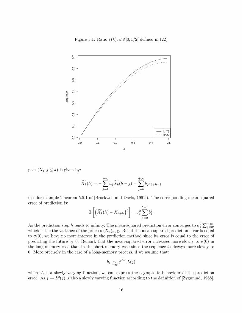
Figure 3.1: Ratio r(k), d ∈]0, 1/2[ defined in (22)

0.0 0.1 0.2 0.3 0.4 0.5

0.0

0.1

0.2

0.3

0.4

0.5

0.6

0.7

d

diffe

renc

e

k=75k=20

past (Xj , j ≤ k) is given by:

Xk(h) = −

+∞∑

j=1

ajXk(h − j) =

+∞∑

j=h

bjεk+h−j

(see for example Theorem 5.5.1 of [Brockwell and Davis, 1991]). The corresponding mean squarederror of prediction is:

E

[(Xk(h) − Xk+h

)2]

= σ2ε

h−1∑

j=0

b2j .

As the prediction step h tends to infinity, The mean-squared prediction error converges to σ2ε

∑+∞j=0,

which is the the variance of the process (Xn)n∈Z. But if the mean-squared prediction error is equalto σ(0), we have no more interest in the prediction method since its error is equal to the error ofpredicting the future by 0. Remark that the mean-squared error increases more slowly to σ(0) inthe long-memory case than in the short-memory case since the sequence bj decays more slowly to0. More precisely in the case of a long-memory process, if we assume that:

bj ∼+∞

jd−1L(j)

where L is a slowly varying function, we can express the asymptotic behaviour of the predictionerror. As j 7→ L2(j) is also a slowly varying function according to the definition of [Zygmund, 1968],

16

b2j = j2d−2L2(j) is ultimately decreasing. The rest of the series and the integral are then equivalent

and we may write:

σ(0) − E

[(Xk(h) − Xk+h

)2]

= σ2ε

+∞∑

j=h

b2j

∼+∞∑

j=h

j2d−2L2(j)

∼

∫ +∞

hj2d−2L2(j)dj

According to Proposition 1.5.10 of [Bingham et al., 1987]:

σ(0) − E

[(Xk(h) − Xk+h

)2]

∼

∫ +∞

hj2d−2L2(j)dj

∼h→+∞

1

1 − 2dh2d−1L2(h) (23)

In the case of a long-memory process with parameter d which verifies bj ∼ jd−1L(j), the convergenceof the mean-squared error to σ(0) is slow as h tends to infinity. On the contrary, for a moving average

process of order q, the sequence σ(0)−E

[(Xk(h) − Xk+h

)2]

is constant and equal to 0 as soon as

h > q. More generally, we can study the case of an ARMA process, which canonical representationis given by:

Φ(Xt) = Θ(εt)

where Φ and Θ are two coprime polynomials with coefficients of degree 0 are equal to 1 and εt is awhite noise. Φ has no root in the unit disk |z| ≤ 1 and Θ has no root in the open disk |z| < 1. bj

is bounded by:|bj | ≤ Cjm−1ρ−j

where ρ is the smallest absolute value of the roots of Φ and m the multiplicity of the correspondingroot (see for example [Brockwell and Davis, 1991] p92). Thus the mean-squared prediction error isbounded by:

σ(0) − E

[(Xk(h) − Xk+h

)2]

= σ2ε

+∞∑

j=h

b2j

≤ σ2εC

2+∞∑

j=h

j2m−2ρ−2j

≤ σ2εC

2+∞∑

j=h

j2m−2 exp (−2j log(ρ))

≤ σ2εC

2

∫ +∞

hj2m−2 exp (−2j log(ρ)) dj

17

By using the substitution t = 2 log(ρ)j ,

σ(0) − E

[(Xk(h) − Xk+h

)2]

≤ σ2εC

2 (2 log(ρ))1−2m∫ +∞

2 log(ρ)ht2m−2 exp (t) dt

≤ σ2εC

2 (2 log(ρ))1−2m Γ(2m − 1, 2 log(ρ)h)

where Γ(., .) is the incomplete Gamma function defined in equation 6.5.3 of [Abramowitz and Stegun, 1984].We know an equivalent of this function:

Γ(2m − 1, 2 log(ρ)h) ∼h→+∞

(2 log(ρ)h)2m−2 exp (2 log(ρ)h)

We conclude that the rate of convergence is exponential. The mean-squared prediction error goesfaster to σ(0) when the predicting process is ARMA than when the process is a long-memoryprocess.The h-step prediction is then more interesting for the long-memory process than for the short-memory process, having observed the infinite past. We consider the truncating effect next.

4.1 Truncated Wiener-Kolmogorov predictor

In practice, we only observe a finite number of samples. We assume now that we only know kobservations (X1, . . . ,Xk). We then define the h-step truncated Wiener-Kolmogorov of order k as:

X ′k(h) = −

h−1∑

j=1

ajX ′k(h − j) −

k∑

l=1

ah−1+jXk+1−j (24)

We now describe the asymptotic behaviour of the mean-squared error of the predictor (24).First we write the difference between the predicting random variable and its predictor:

X ′k(h) − Xk+h = −

h−1∑

j=1

ajX′k(h − j) −

k∑

l=1

ah−1+jXk+1−j − εk+h +

+∞∑

j=1

ajXk+h−j

= −εk+h +

h−1∑

j=1

aj

(Xk+h−j − X ′

k(h − j))

+

k∑

j=1

ah−1+j (Xk+1−j − Xk+1−j)

+

+∞∑

j=k+1

ah−1+jXk+1−j

= −εk+h +h−1∑

j=1

aj

(Xk+h−j − X ′

k(h − j))

++∞∑

j=k+1

ah−1+jXk+1−j

We will use the process of induction on h to show that

X ′k(h) − Xk+h = −

h−1∑

l=0

∑

j1+j2+...+jh=l

(−1)card(j,j 6=0)aj1aj2 . . . ajh

εk+h−l

+

+∞∑

j=k+1

∑

i1+i2+...+ih=h−1

(−1)card(il ,il 6=0,l>1)aj+i1ai2 . . . aih

Xk+1−j.

18

For h = 2, we have for example

X ′k(2) − Xk+2 = −(a0εk+2 − a1εk+1) +

+∞∑

j=k+1

(−a1aj + aj+1)Xk+1−j .

Let A(z) and B(z) denote A(z) = 1 +∑+∞

j=1 ajzj and B(z) = 1 +

∑+∞j=1 bjz

j . Since we have

A(z) = B(z)−1, we obtain the following conditions on the coefficients:

b1 = −a1

b2 = −a2 + a21

b3 = −a3 + 2a1a2 − a31

. . .

So we obtain:

X ′k(h) − Xk+h = −

h−1∑

l=0

blεk+h−l ++∞∑

j=k+1

h−1∑

m=0

aj+mbh−1−mXk+1−j. (25)

Since the process (εn)n∈Z is uncorrelated and then the two terms of the sum (25) are orthogonal,we can rewrite the mean-squared error:

E

[X ′

k(h) − Xk+h

]2=

h−1∑

l=0

b2l σ

2ε (26)

+E

+∞∑

j=k+1

(h−1∑

m=0

aj+h−1−mbm

)Xk+1−j

2

. (27)

The first part of the error (26) is due to the prediction method and the second (27) due to thetruncating of the predictor. We now approximate the error term (27) by using (3) and (4). Weobtain the following upper bound:

∀δ > 0,

∣∣∣∣∣

h−1∑

m=0

aj+h−1−mbm

∣∣∣∣∣ ≤h−1∑

m=1

|aj+h−1−mbm| + |b0aj+h−1|

≤ C1C2

∫ h

0(j + h − 1 − l)−d−1+δld−1+δdl + C1(j + h)−d−1

≤ C1C2h−1+2δ

∫ 1

0

(j

h+ 1 − l

)−d−1+δ

ld−1+δdl + C1(j + h)−d−1

≤ C1C2h−1+2δj−d−1+δ

∫ 1

0

(1

h+

1 − l

j

)−d−1+δ

ld−1+δdl + C1(j + h)−d−1

≤ C1C2hd+2δj−d−1+δ

∫ 1

0ld−1+δdl + C1(j + h)−d−1

∣∣∣∣∣

h∑

m=0

aj+h−mbm

∣∣∣∣∣ ≤ C1C2hd+2δ

dj−d−1+δ (28)

19

This bound is in fact an asymptotic equivalent for the fractionally integrated process F(d) because,in that case, the sequences aj and bj have a constant signs. Using Proposition 2.2.1 for the one-stepprediction and we have:

Proposition 4.1.1. Let (Xn)n∈Z be a linear stationary process defined by (1), (2) and possessing

the features (3) and (4). We can approximate the mean-squared prediction error of X ′k(1) by:

∀δ > 0, E

[X ′

k(h) − Xk+h

]2=

h−1∑

l=0

b2l σ

2ε + O

(h2d+δk−1+δ

). (29)

Having k observations, we search for the step h for which the variance of the predictor has forupper bound σ(0). Then the prediction error have for asymptotic bound O

(h2dk−1

). We want to

choose h to have the prediction error negligible with respect to the information given by the linearleast-squares predictor given the infinite past (see (23)) and we obtain:

h2dk−1 = o(h2d−1)

and then h = o(k). With the truncated Wiener-Kolmogorov predictor, it is interesting to computethe h-step predictor if we have k observations h = o(k).

4.2 The k-th Order Linear Least-Squares Predictor

For next step predictor, when we fitted an autoregressive process, we search the linear least-squarespredictor knowing the finite past (X1, . . . ,Xk) and the predictor is then the projection of the random

variable onto the past. Let Xk(h) denote the projection of Xk+h onto the span of (X1, . . . ,Xk).

Xk(h) verifies the recurrence relationship

Xk(h) = −

k∑

j=1

aj,kXk(h − j)

where Xk(h − j) is the direct linear least-squares predictor of Xk+h−j based on the finite past(X1, . . . ,Xk). By induction, we obtain the predictor as a function of (X1, . . . ,Xk): For next stepprediction by fitting an autoregressive process, the best linear least-squares predictor knowing thefinite past is a projection of the random variable Xk+1 onto the past.

Xk(h) = −

k∑

j=1

cj,kXk+1−j.

Since Xk(h) is the projection of Xk+h onto (X1, . . . ,Xk) in L2, the vector (cj,k)1≤j≤k minimizes themean-squared error:

E

[Xk(h) − Xk+h

]2=

∫ π

−πf(λ)

∣∣∣∣∣∣exp(iλ(h − 1)) +

k∑

j=1

cj,k exp(−iλj)

∣∣∣∣∣∣

2

dλ

The vector (cj,k)1≤j≤k is a solution of the equation:

∇c E

[Xk(h) − Xk+h

]2= 0

20

where ∇c is the gradient. The vector (cj,k)1≤j≤k is then equal to:

(cj,k)1≤j≤k = −Σ−1k (σh−1+j)1≤j≤k. (30)

The corresponding mean squared error of prediction is given by:

E

[Xk(h) − Xk+h

]2=

∫ π

−πf(λ)

∣∣∣∣∣∣exp(iλ(h − 1)) +

k∑

j=1

cj,k exp(−iλj)

∣∣∣∣∣∣

2

dλ

= σ(0) + 2

k∑

j=1

cj,kσ(h − 1 + j) +

k∑

j,l=1

cj,kcl,kσ(j − l)

= σ(0) + 2 t(cj,k)1≤j≤k(σh−1+j)1≤j≤k + t(cj,k)1≤j≤kΣk(cj,k)1≤j≤k

= σ(0) − t(σh−1+j)1≤j≤kΣ−1k (σh−1+j)1≤j≤k

The matrix Σ−1k is symmetric positive definite and the prediction error of this method is always

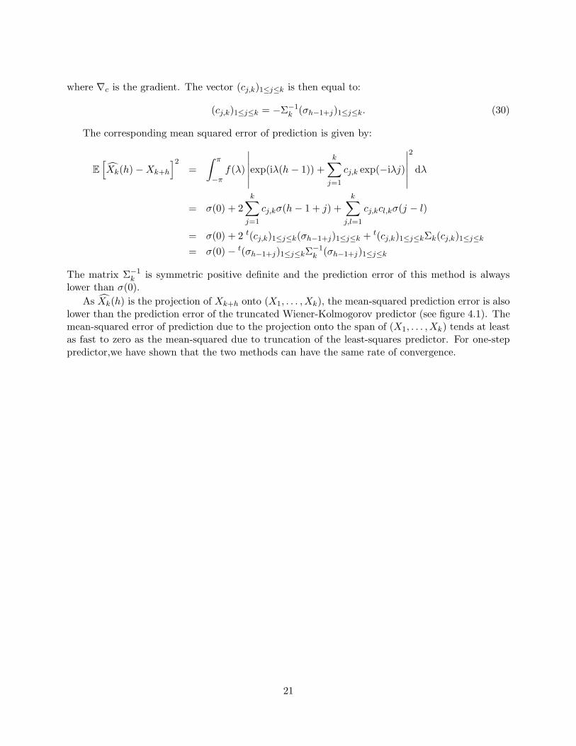
lower than σ(0).

As Xk(h) is the projection of Xk+h onto (X1, . . . ,Xk), the mean-squared prediction error is alsolower than the prediction error of the truncated Wiener-Kolmogorov predictor (see figure 4.1). Themean-squared error of prediction due to the projection onto the span of (X1, . . . ,Xk) tends at leastas fast to zero as the mean-squared due to truncation of the least-squares predictor. For one-steppredictor,we have shown that the two methods can have the same rate of convergence.

21

Figure 4.1: Mean-squared error of Xk(h) (MMSE), X ′k(h) (TPMSE) and Xk(h) (LLSPE) for d = 0.4

and k = 80

0 50 100 150

0.0

0.2

0.4

0.6

0.8

1.0

h

erre

ur

0

MMSETPMSELLSPE

References

[Abramowitz and Stegun, 1984] Abramowitz, M. and Stegun, I. (1984). Handbook of mathematicalfunctions with formulas, graphs, and mathematical tables. . A Wiley-Interscience Publication. Se-lected Government Publications. New York: John Wiley & Sons, Inc; Washington, D.C.: NationalBureau of Standards. .

[Bhansali, 1978] Bhansali, R. (1978). Linear prediction by autoregressive model fitting in the timedomain. Ann. Stat., 6:224–231.

[Bhansali and Kokoszka, 2001] Bhansali, R. and Kokoszka, P. (2001). Prediction of long-memorytime series: An overview. Estadıstica 53, No.160-161, 41-96.

[Bingham et al., 1987] Bingham, N., Goldie, C., and Teugels, J. L. (1987). Regular variation.

[Brockwell and Davis, 1988] Brockwell, P. and Davis, R. (1988). Simple consistent estimation ofthe coefficients of a linear filter. Stochastic Processes and their Applications.

[Brockwell and Davis, 1991] Brockwell, P. and Davis, R. (1991). Time Series : Theory and Methods.Springer Series in Statistics.

22

[Granger and Joyeux, 1980] Granger, C. and Joyeux, R. (1980). An introduction to long-memorytime series models and fractional differencing. J. Time Ser. Anal., 1:15–29.

[Inoue, 1997] Inoue, A. (1997). Regularly varying correlation functions and KMO-Langevin equa-tions. Hokkaido Math. J., 26(2):457–482.

[Inoue, 2000] Inoue, A. (2000). Asymptotics for the partial autocorrelation function of a stationaryprocess. J. Anal. Math., 81:65–109.

[Lewis and Reinsel, 1985] Lewis, R. and Reinsel, G. (1985). Prediction of multivariate time seriesby autoregressive model fitting. Journal of multivariate analysis.

[Mandelbrot and Wallis, 1969] Mandelbrot, B. and Wallis, J. (1969). Some long-run properties ofgeophysical records. Water Resource Research, 5:321–340.

[Ray, 1993] Ray, B. (1993). Modeling long-memory processes for optimal long-range prediction. J.Time Ser. Anal., 14(5):511–525.

[Whittle, 1963] Whittle, P. (1963). Prediction and regulation by linear least-square methods. 2nded.

[Yajima, 1993] Yajima, Y. (1993). Asymptotic properties of estimates in incorrect ARMA modelsfor long- memory time series. In New directions in time series analysis. Part II. Proc. Workshop,Minneapolis/MN (USA) 1990, IMA Volumes in Mathematics and Its Applications 46, 375-382.

[Zygmund, 1968] Zygmund, A. (1968). Trigonometric series. Cambridge University Press.

23