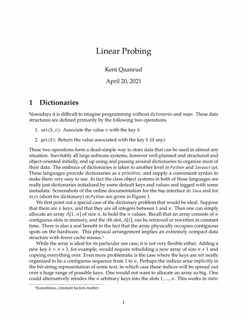
Linear Probing

Kent Quanrud

April 20, 2021

1 DictionariesNowadays it is difficult to imagine programming without dictionaries and maps. These datastructures are defined primarily by the following two operations.

1. set(:,E): Associate the value E with the key :.

2. get(:): Return the value associated with the key : (if any).

These two operations form a dead-simple way to store data that can be used in almost any

situation. Inevitably all large software systems, however well-planned and structured and

object-oriented initially, end up using and passing around dictionaries to organize most of

their data. The embrace of dictionaries is taken to another level in Python and Javascript.

These languages provide dictionaries as a primitive, and supply a convenient syntax to

make them very easy to use. In fact the class object systems in both of these languages are

really just dictionaries initialized by some default keys and values and tagged with some

metadata. Screenshots of the online documentation for the Map interface in Java and for

dict (short for dictionary) in Python are given in Figure 1.

We first point out a special case of the dictionary problem that would be ideal. Suppose

that there are = keys, and that they are all integers between 1 and =. Then one can simply

allocate an array �[1..=] of size =, to hold the = values. Recall that an array consists of =

contiguous slots in memory, and the 8th slot, �[8], can be retrieved or rewritten in constant

time. There is also a real benefit to the fact that the array physically occupies contiguous

spots on the hardware. This physical arrangement implies an extremely compact data

structure with fewer cache misses.1

While the array is ideal for its particular use case, it is not very flexible either. Adding a

new key : = = + 1, for example, would require rebuilding a new array of size = + 1 and

copying everything over. Even more problematic is the case where the keys are not neatlyorganized to be a contiguous sequence from 1 to =. Perhaps the indices arise implicitly inthe bit-string representation of some text, in which case these indices will be spread out

over a huge range of possible keys. One would not want to allocate an array so big. One

could alternatively reindex the = arbitrary keys into the slots 1, ..., =. This works in static

1Sometimes, constant factors matter.

1

Java Map Interface Python Dictionary

Figure 1: The Map interface in Java (left) and the built-in Dictionary data structure in Python

(right).

situations where the keys are presented at the beginning and never change thereafter. But

recall that the primary appeal of dictionaries is their flexibility, and their ability to handle

all sorts of different keys, without foresight.A deterministic way to implement dictionaries is via search trees. If the keys are

comparable (such as numbers, or strings in alphabetical order), then search trees can

organize the data in sorted order in a tree-like data structure. With a well-designed search

tree, searching for a key has roughly the performance of a binary search over a sorted

array: $(log =

)time per get and set. These data structures are often ingenious. Red-black

trees use one-bit markers at each node to detect if a subtree has become too “tilted” in

one way or another, and rebuilds the tilted portion whenever this occurs. Lazy rebuilding

explicitly counts the number of keys in each subtree, and rebuilds an entire subtree when

one child subtree becomes much larger than the other. The celebrated splay tree datastructure by Sleator and Tarjan [9] readjusts itself with every get and set operation and

achieves $(log =

)amortized time (i.e., $

(: log =

)time for any sequence of : operations).

Another deterministic approach to dictionaries is tries, which requires the keys to be (fairly

2

short) bit strings, and uses each successive bit to dictate which direction to go down a

binary tree. By compressing long paths in these trees (such as in Patricia tries [3]), these

algorithms can be compact and efficient. Now, as clever as these data structures are, they

suffer some drawbacks compared to arrays. The $(log =

)query time for search trees is a

bit higher then the $(1) time of arrays2. They are more complicated to implement, and

require a lot of pointer chasing, which leads to many cache misses on the CPU.3

We instead consider simpler randomized approaches to the dictionary problem; namely,

hash tables. Hash tables combines the dynamic flexibility of search trees with the raw

efficiency of arrays. The only drawback is that the performance guarantees are randomized,

which requires a little more sophistication in the analysis. But most people consider the net

tradeoff to be easily beworth it. Hash tables are generally based on the following framework.

Suppose that there are = keys :1, . . . , := from the set of integers [*] = {1, . . . , *}, where*

is typically incredibly large. One allocates an array �[1..<] of size < (typically < = $(=)),and randomly constructs a hash function ℎ : [*] → [<]. Ideally, each key-value pair (:8 , E8)is stored in the slot �[ℎ(:8)]. The remaining question is what to do when keys collide, i.e.,when ℎ(:′) = ℎ(:′′) for two distinct keys :′ and :′′. There are various ways, sometimes

simple and sometimes clever, to account for collisions, such as the following.

1. Make ℓ so large that even a single collision is unlikely. Exercise 1 studies how large <

needs to be (relative to =) for this to occur.

2. For each slot 9 ∈ [ℓ ] in the hash table, build a linked list of all keys that hash to slot 9.

We study this first in Section 2.

3. For each slot 9 ∈ [ℓ ] in the hash table, build a second hash table (this time following

strategy 1) for all keys that hash to slot 9. This is the topic of Exercise 3.

4. Suppose we want to insert a key :. Make two hash keys, ℎ1(:) and ℎ2(:), and hope

that one of these two hash keys is open. More radically, if ℎ1(:) and ℎ2(:) are occupiedby other keys, see if it is possible to move one of these other keys to its own extra hash

key, possibly bumping more keys recursively. This wild approach is called cuckoohashing.

5. Suppose we want to insert a key : and �[ℎ(:)] is occupied. We start scanning the

array �[ℎ(:) + 1], �[ℎ(:) + 2], . . . until we find the first empty slot, and put : there

instead. This approach is called linear probing, and will be the topic of the second half

of our discussion.

Ignoring the possibility of collisions, these hash tables have the appeal of potentially

being constant time, like an array. Given a key, the hash code ℎ(:) gives a direct index into

an array. If the key is there, then we are done. While there may be collisions, we can see in

each of the strategies above that �[ℎ(:)] still gets us very “close” to the final location of :.

Maybe we have to traverse a short list, hash into a secondary hash table, or continue to

scan � until we find our key. For each of these algorithms, some probabilistic analysis is

required to understand how much time the “collision-handling” stage will take.

2Sometimes, log factors matter.

3This last point can be helped to some extent by cache-oblivious versions.

3

One final remark about the size of hash tables: above, we acted as if we knew a priori thenumber of keys that will be put in the table, and used this to choose the size of the array �.

Sometimes, that is the case, but oftentimes it is not, and again the point of dictionary data

structures is to not have to plan for these things ahead of time. The easy way to handle

an unknown number of keys is by the doubling trick. We start with 0 keys and a modestly

sized array �; say, of size 64. Whenever the number of keys approaches a constant fraction

of the capacity (say, 16), we double the size of the array (to 128). This means we allocate a

new array �′ with double the capacity, scan the previous array �, and rehash each of the

items into �′. A simple amortized analysis shows that the extra effort spent rebuilding is

neglible. (This is the same strategy used, for example, in Java’s ubiquitous ArrayList data

structure.) We note that there are some distributed computational settings where one wants

to maintain a distributed dictionary, and where simply rehashing items becomes expensive

and impractical. We refer the reader to a technique called consistent hashing that addresses

this challenge [1]. Distributed dictionaries are particularly useful for caching on the web.

2 Hash tables with chainingWe first consider hash tables that use linked lists to handle collisions. These are maybe the

easiest to analyze, and also are most similar in spirit to the count-min-sketch data structure

previously discussed.

We recall the basic framework. We have = distinct keys :1, . . . , := , from a universe

of integers {1, . . . , *}. We allocate an array �[1..<] of size <. (Eventually we will set

< = $(=), but for the moment we leave it as a variable to explore the tradeoffs between

larger and smaller <.)

We randomly construct a hash fucntion ℎ : [*] → [<]. Here we analyze the setting

where ℎ is a universal hash function, but later we will also explore stronger notions of

independence. Exercise 2 explores the setting where ℎ is an ideal hash function.

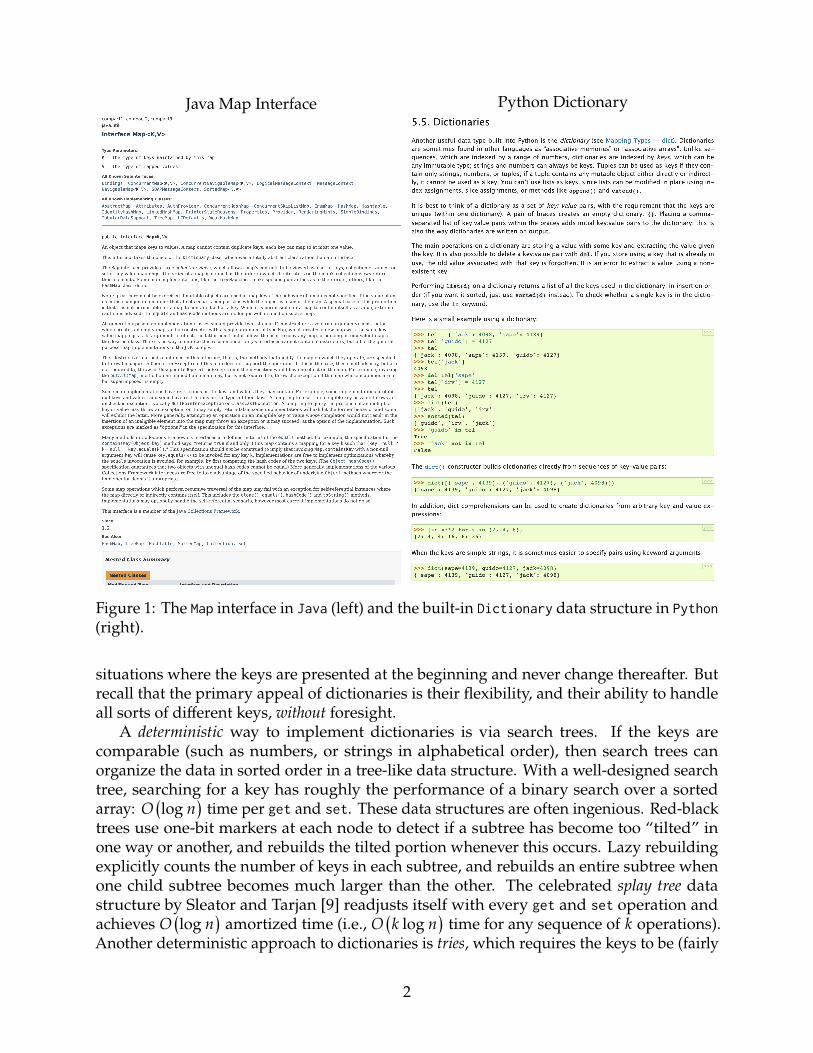
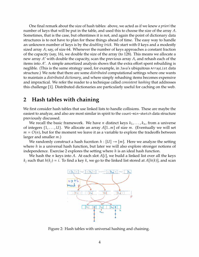
We hash the = keys into �. At each slot �[8], we build a linked list over all the keys

: 9 such that ℎ(: 9) = 8. To find a key :, we go to the linked list stored at �[ℎ(:)], and scan

Figure 2: Hash tables with universal hashing and chaining.

4

the linked list looking for key :. A high level diagram of the scheme is given in Figure 2.

Clearly, the running time of each get and setwill be proportional to the length of the list at

the hashed array index. Thus most of our analysis will focus on the lengths of these lists.

We first recall the definition of a universal hash function.

Definition 2.1. A randomly constructed function ℎ : [=] → [<] is universal if, for any twoindices 81 ≠ 82, we have

P[ℎ(81) = ℎ(82)] =1

<.

We also remind the reader that a universal hash function can be constructed as a random

function of the form ℎ(G) = (0G + 1 mod ?) mod <, where ? is a prime number larger

than the maximum possible key.

Theorem 2.2. Consider chaining with = keys, an array �[1, ..., <], and a universal hash functionℎ : [*] → [<]. Then each get and set takes $(1 + =/<) time in expectation. In particular,for < = $(=), hash tables with chaining takes $(=) total space and $(1) time per operation inexpectation.

Proof. The time to insert a key : is proportional to the number of collisions with : (plus

$(1)). The expected number of collisions

E[|:′ : ℎ(:′) = ℎ(:)|] (a)=∑:′≠:

P[ℎ(:′) = ℎ(:)] (b)=∑:′≠:

1

<

(c)== − 1

<

Here (a) is by linearity of expectation. (b) is by universality. (c) is because there are = − 1

other keys. �

3 4-wise independenceA collection of = variables -1, . . . , -= is k-wise independent if for any : variables

-81 , . . . , -8: , and values H1, H2, . . . , H: , we have

P[-81 = H1, -82 = H2, · · · , -8: = H:

]= P[-81 = H1]P[-82 = H2] · · ·P

[-8: = H:

].

Lemma 3.1. Let -1, . . . , -: be :-wise independent random variables. Then

E[-1-2 · · ·-:] = E[-1]E[-2] · · ·E[-:].

Before proving Lemma 3.1, let us give a simple example where :-wise independence

matters. Let -1, · · · , -: ∈ {0, 1} where each -8 denotes the outcome of a fair coin toss -

0 for tails, 1 for heads. Then -1 · · ·-: = 1 if all of the coin tosses come up heads, and 0

otherwise. Consider the following parallel universes.

1. Suppose each -8 was based on a different, independent coin toss. That is, -1, . . . , -:are mutually independent. The probability that : independent coin tosses all comes

up heads is 1/2: , so E[-1 · · ·-:] = 1/2: .

5

2. Suppose each -8 was based on the same coin toss. That is, -1 = · · · = -: ; they

are certainly not independent. Then the probability that all -1, . . . , -: = 1 is the

probability of a single coin coming up heads, 1/2, and so E[-1 · · ·-:] = 1/2.

Here there is an exponential gap between independent and non-independent coin tosses.

Proof of Lemma 3.1. We have

E[-1-2 · · ·-:](a)=

∑H1 ,H2 ,...,H:

H1H2 · · · H: P[-1 = H1, -2 = H2, . . . , -: = H:]

(b)=

∑H1 ,H2 ,...,H:

H1H2 · · · H: P[-1 = H1]P[-2 = H2] · · ·P[-: = H:]

=

(∑H1

H1 P[-1 = H1]) (∑

H2

H2 P[-2 = H2])· · ·

(∑H:

H: P[-: = H:])

(c)= E[-1]E[-2] · · ·E[-:].

Here (a) is by definition of expectation4. (b) is by :-wise independence. (c) is by definition

of expectation, for each -8 . �

A concentration inequality for 4-wise independent sums. Recall Markov’s inequality:

the probability of a nonnegative random variable, - ≥ 0, being at least twice its expected

value, is at most 1/2. Here we consider an analogous but stronger inequality for sums of

4-wise independent random variables.

Lemma 3.2. Let -1, -2, . . . , -= ∈ {0, 1} be 4-wise independent variables where for each 8,E[-8] = ?. Let � = ?= = E

[∑=8=1-8

]. Then for any � > 0,

P

[=∑8=1

-8 ≥ � + �]≤� + 3�2

�4

.

Before proving Lemma 3.2, let us compare it to Markov’s inequality. Given -1, . . . , -=and � as in Lemma 3.2, Markov’s inequality say that for all > 0,

P[-1 + · · · + -= ≥ (1 + )�] ≤1

1 + . (1)

Lemma 3.2 says that

P[-1 + · · · + -= ≥ (1 + )�](d)≤ � + 3�2

4�4

≤ 3

2�4

. (2)

4We are summing over all possible outcomes (H1 , . . . , H:) of (-1 , . . . , -:), multiplying the value, H1 · · · H: ,with the probability of the outcome, P[-1 = H1 , . . . , -: = H:].

6

Here (d) applies Lemma 3.2 with � = �. Compare the RHS of (1) with the RHS of (2). In

(2), the upper bound is decreasing in at a 1/ 4, compared 1/ in (1). Moreover, (2) is

decreasing in the expected value � at a rate of 1/�2. That is, the greater the mean, the smaller

the probability of deviated from the mean. This is our first example of a concentration inequality.We will soon see why this helpful when we return to designing hash tables after proving

Lemma 3.2.

Proof of Lemma 3.2. We have

P

[=∑8=1

-8 ≥ � + �]= P

[=∑8=1

-8 − � ≥ �

](a)= P

(=∑8=1

-8 − �)

4

≥ �4

(b)≤

E[ (∑=

8=1-8 − �

)4

](� − �)4

.

The key step is (a), where we raise both sides to the fourth power. (b) is by Markov’s

inequality. We claim that

E(=∑8=1

-8 − �)

4 ≤ � + 3�2,

which would complete the proof. We first have

E(=∑8=1

-8 − �)

4 = E(=∑8=1

(-8 − ?))

4because � = ?=. Now,

(∑=8=1(-8 − ?)

)4

expands out to the sum

=∑8=1

(-8 − ?)4 +(4

2

) ∑8< 9

(-8 − ?)2(-9 − ?

)2 +

(monomials w/ some

(-8 − ?) w/ degree 1

). (3)

Some examples of the third category would be (-1 − ?)3(-2 − ?), (-1 − ?)2(-2 − ?)(-3 − ?),and (-1−?)(-2−?)(-3−?)(-4−?). Consider the expected value of each of these categories

of monomials.

1. For each 8, we have

E[(-8 − ?)4

]= ?(1 − ?)4 + (1 − ?)?4 ≤ ?(1 − ?).

2. For each 8 ≠ 9, we have

E[(-8 − ?)2

(-9 − ?

)2

] (c)= E

[(-8 − ?)2

]E[ (-9 − ?

)2

] (d)≤ ?2(1 − ?)2.

Here (c) is because of pairwise independence. (d) is because

E[(-8 − ?)2

]= ?(1 − ?)2 + (1 − ?)?2 ≤ ?(1 − ?).

7

3. Eachmonomial in the third category has expected value 0. This is because we can pull

out the degree 1 term by independence, which has expected value 0. For example,

E[(-1 − ?1)3(-2 − ?2)

] (e)= E

[(-1 − ?1)3

]E[-2 − ?2] = 0,

where (e) is by pairwise independence, and (f) is because E[-2 − ?2] = 0.

Plugging back in to above, we have

E(=∑8=1

-8 − �)

4 = =?(1 − ?) +(=

2

) (4

2

) (?2(1 − ?)2

)≤ =? + 3(=?)2,

as desired. �

Remark 3.1. The claim would hold even for -8 not identically distributed (as long as they

are 4-wise independent and are each in [0, 1]). This restricted setting suffices for our

applications and simplifies the exposition.

3.1 Hashing with linked lists with 4-wise independent functionsRecall the hash tables with chaining. If we use a 4-wise independent hash function rather

than a universal hash function, then we get better bounds. In general, the bounds improve

with more independence.

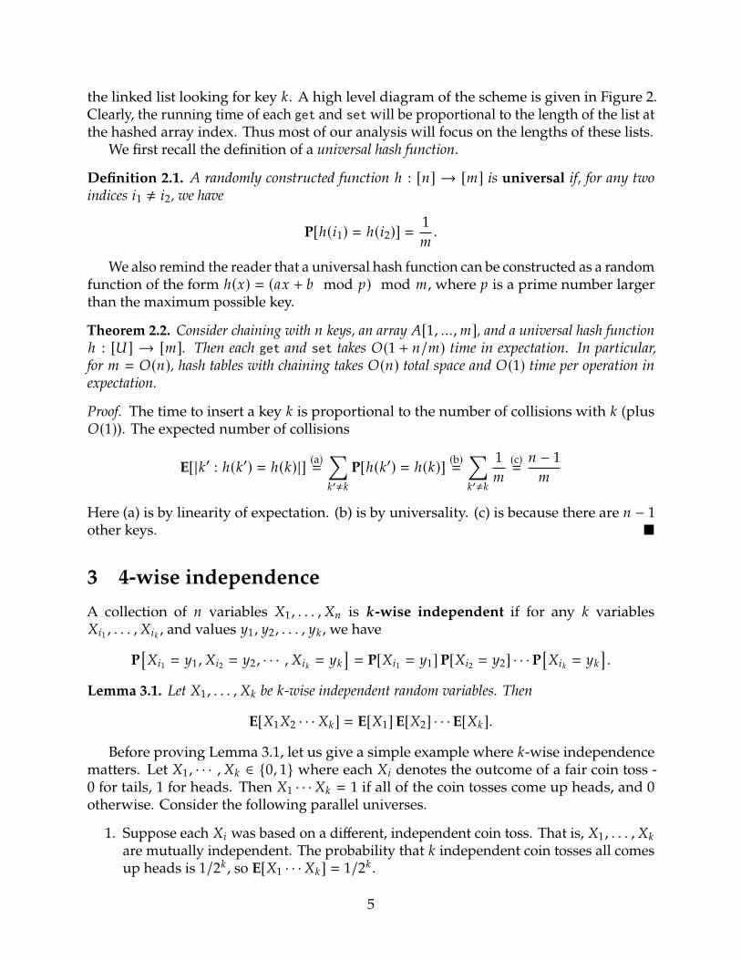
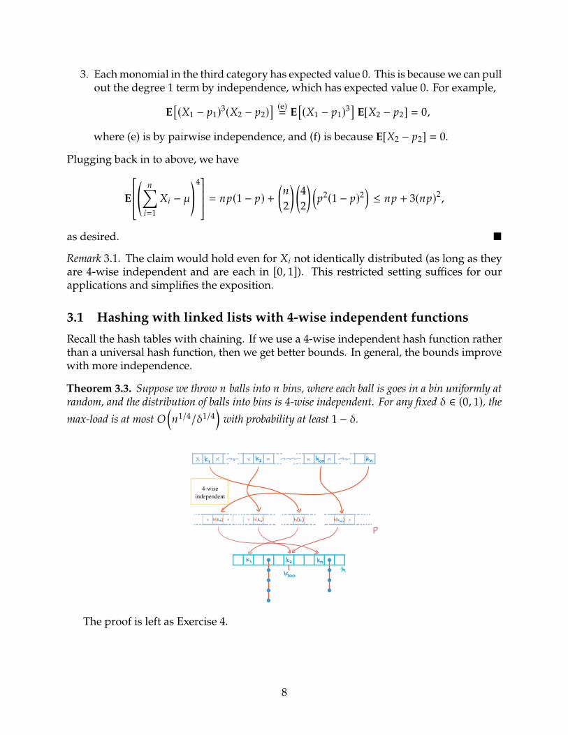
Theorem 3.3. Suppose we throw = balls into = bins, where each ball is goes in a bin uniformly atrandom, and the distribution of balls into bins is 4-wise independent. For any fixed � ∈ (0, 1), themax-load is at most $

(=1/4/�1/4

)with probability at least 1 − �.

X K X M X K2 nm x Hoo m kn

insdepint

x hash x x hCkz hKp Khoo x

P

k ka knm

Koo

4-wiseindependent

The proof is left as Exercise 4.

8

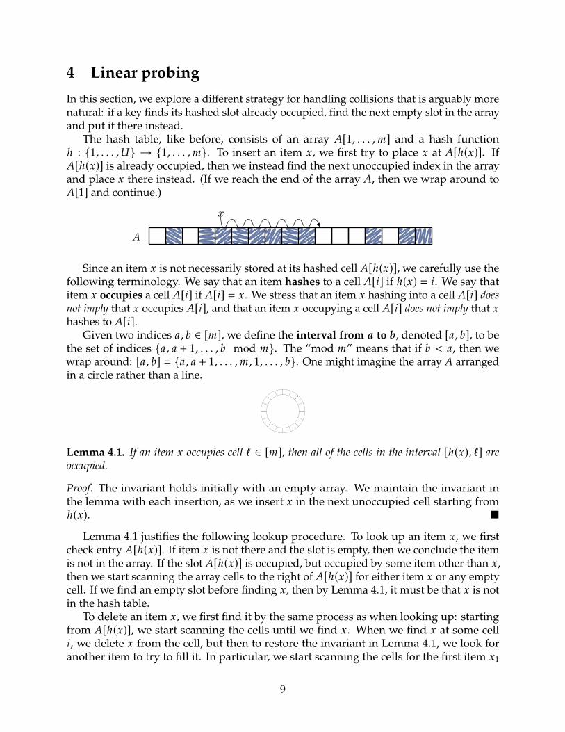
4 Linear probingIn this section, we explore a different strategy for handling collisions that is arguably more

natural: if a key finds its hashed slot already occupied, find the next empty slot in the array

and put it there instead.

The hash table, like before, consists of an array �[1, . . . , <] and a hash function

ℎ : {1, . . . , *} → {1, . . . , <}. To insert an item G, we first try to place G at �[ℎ(G)]. If

�[ℎ(G)] is already occupied, then we instead find the next unoccupied index in the array

and place G there instead. (If we reach the end of the array �, then we wrap around to

�[1] and continue.)

x<latexit sha1_base64="6wjan1T45mpXiU9JH+gKmbxfiH0=">AAACZnicbVHLTttAFB0bWh5taQAhFmxGRJVYRTZFguyQuukOIjWAlFhoPLlORszDmrmGRpa/oNv24/oH/QzGjoUawpFmdHTuuY+Zm+ZSOIyiv0G4tv7u/cbm1vaHj592Pnd2926cKSyHITfS2LuUOZBCwxAFSrjLLTCVSrhNH77V8dtHsE4Y/QPnOSSKTbXIBGfopcHP+0436kUN6CqJW9IlLa7vd4Or8cTwQoFGLplzozjKMSmZRcElVNvjwkHO+AObwshTzRS4pGwmregXr0xoZqw/Gmmj/p9RMuXcXKXeqRjO3OtYLb4VGxWYXSSl0HmBoPmiUVZIiobWz6YTYYGjnHvCuBV+VspnzDKO/nOWutS1rcucr1HP2bTidsWSpkZ6C209tVDG1bJNQoZWTGfodQ1P3CjF9KQcQ+6q5hbS6KpZQb8BXZDzs5b045cV3Jz24q+908FZ9/KkXcYmOSLH5ITE5Jxcku/kmgwJJ0B+kd/kT/Av3AkPwsOFNQzanH2yhJA+A/p4vJ8=</latexit>

A<latexit sha1_base64="DC/qdQlZgHusAbleDmSKJF3LdWA=">AAACZnicbVHLattAFB0pfThu6yYtpYtuhppCVkZKA0l2Kd10Vwfi2GALMxpf2YPnIWauGozQF2SbfFz/oJ/RkSxC3PTADIdzz33M3DSXwmEU/Q7CvWfPX7zs7HdfvX7Te3tw+O7amcJyGHEjjZ2kzIEUGkYoUMIkt8BUKmGcrr/X8fEvsE4YfYWbHBLFllpkgjP00uW3+UE/GkQN6FMSt6RPWgznh8HP2cLwQoFGLplz0zjKMSmZRcElVN1Z4SBnfM2WMPVUMwUuKZtJK/rFKwuaGeuPRtqojzNKppzbqNQ7FcOV+zdWi/+LTQvMzpJS6LxA0HzbKCskRUPrZ9OFsMBRbjxh3Ao/K+UrZhlH/zk7Xera1mXO16jnbFpx+8SSpkZ6C209tVDG1a5NQoZWLFfodQ033CjF9KKcQe6q5hbS6KpZwXkDuiWnJy05jx9WcH08iL8Oji9P+hdH7TI65BP5TI5ITE7JBflBhmREOAFyS+7IffAn7IUfwo9baxi0Oe/JDkL6F4wKvGg=</latexit>

Since an item G is not necessarily stored at its hashed cell �[ℎ(G)], we carefully use the

following terminology. We say that an item hashes to a cell �[8] if ℎ(G) = 8. We say that

item G occupies a cell �[8] if �[8] = G. We stress that an item G hashing into a cell �[8] doesnot imply that G occupies �[8], and that an item G occupying a cell �[8] does not imply that G

hashes to �[8].Given two indices 0, 1 ∈ [<], we define the interval from a to b, denoted [0, 1], to be

the set of indices {0, 0 + 1, . . . , 1 mod <}. The “mod <” means that if 1 < 0, then we

wrap around: [0, 1] = {0, 0 + 1, . . . , <, 1, . . . , 1}. One might imagine the array � arranged

in a circle rather than a line.

Lemma 4.1. If an item G occupies cell ℓ ∈ [<], then all of the cells in the interval [ℎ(G), ℓ ] areoccupied.

Proof. The invariant holds initially with an empty array. We maintain the invariant in

the lemma with each insertion, as we insert G in the next unoccupied cell starting from

ℎ(G). �

Lemma 4.1 justifies the following lookup procedure. To look up an item G, we first

check entry �[ℎ(G)]. If item G is not there and the slot is empty, then we conclude the item

is not in the array. If the slot �[ℎ(G)] is occupied, but occupied by some item other than G,

then we start scanning the array cells to the right of �[ℎ(G)] for either item G or any empty

cell. If we find an empty slot before finding G, then by Lemma 4.1, it must be that G is not

in the hash table.

To delete an item G, we first find it by the same process as when looking up: starting

from �[ℎ(G)], we start scanning the cells until we find G. When we find G at some cell

8, we delete G from the cell, but then to restore the invariant in Lemma 4.1, we look for

another item to try to fill it. In particular, we start scanning the cells for the first item G1

9

with ℎ(G1) ≤ 8, or else an empty cell. If we find such an item G1 in a cell 81, then we put it in

the cell 8 where G was deleted from. We then continue scanning for an item to replace 81,

and so forth.

This hashing scheme is called linear probing, and has a special place in the history

of computer science. It was analyzed by Donald Knuth in 1964 [2]. Knuth is sometimes

called the “father of the analysis of algorithms”, and he is credited with formalizing the

subject and popularizing $-notation.5 As Knuth tells it6, this was the first algorithm he

ever formally analyzed, and therefore, arguably, the first algorithm that anyone has ever(so) formally analyzed. He showed that for ideal hash functions, the expected time of any

operation is $((=/(< − =))2

); in particular, a constant, whenever < is bigger than = by a

constant factor. This data structure also works very well in practice, even if hash functions

in practice are not truly independent. Part of that is owed to the simplicity of the data

structure. Scanning an array is extremely fast on hardware, and much faster than chasing

pointers along a linked list.

Post-Knuth, there remained a question of how much independence was required to get

constant running time in expectation. Around 1990, Schmidt and Siegel [7, 8] showed that

$(log =

)-wise independence sufficed7. Then, in 2007, Pagh, Pagh, and Ruzic [5] showed

that (just!) 5-wise independence sufficed. This was dramatic progress for arguably the

oldest problem in algorithm design. Soon after, [6] showed that 4-wise independence was

not enough. So the answer is 5!

Here we give a simplified analysis of the result of [5]. We don’t put too much emphasis

on the constants, preferring to keep the main ideas as clear as possible. Much better

constants can be found in [5] and also the reader is encouraged to refine the analysis

themselves. Other proofs of the constant time bound can be found in [4, 10].

Theorem 4.2. Let ℎ be 5-wise independent. For < ≥ 8=, linear probing takes expected constanttime per operation.

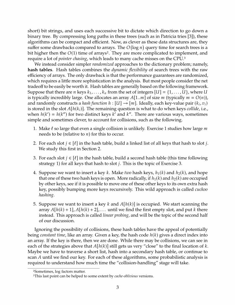
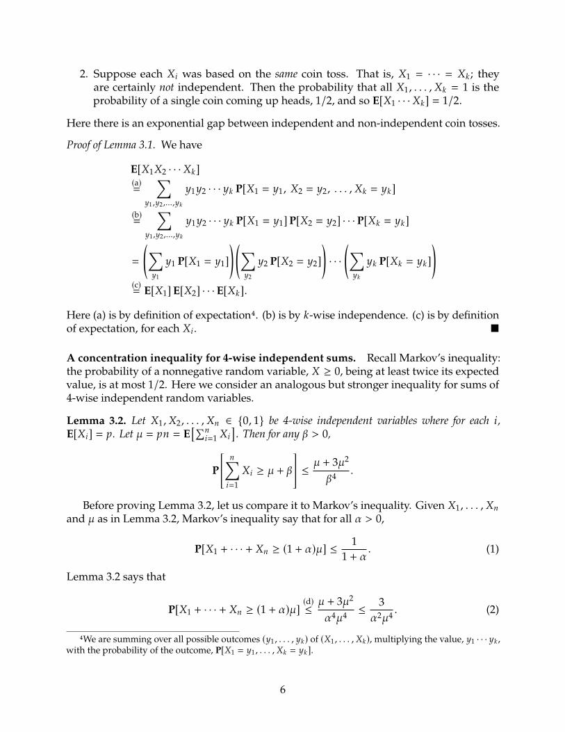
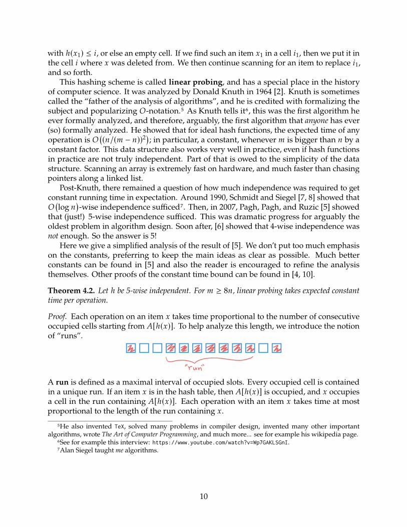
Proof. Each operation on an item G takes time proportional to the number of consecutive

occupied cells starting from �[ℎ(G)]. To help analyze this length, we introduce the notion

of “runs”.Run

Z Z Z Z Z Z Z Z Z

run

run of length kK items hashed into k slots

A run is defined as a maximal interval of occupied slots. Every occupied cell is contained

in a unique run. If an item G is in the hash table, then �[ℎ(G)] is occupied, and G occupies

a cell in the run containing �[ℎ(G)]. Each operation with an item G takes time at most

proportional to the length of the run containing G.

5He also invented TeX, solved many problems in compiler design, invented many other important

algorithms, wrote The Art of Computer Programming, and much more... see for example his wikipedia page.

6See for example this interview: https://www.youtube.com/watch?v=Wp7GAKLSGnI.7Alan Siegel taught me algorithms.

10

Let 8 = ℎ(G), and let ' be the run at index 8. Note that ' and its length |' | are random.

We have

E[

running time

(up to constants)

]≤ E[|' |] =

=∑ℓ=1

ℓ P[|' | = ℓ ]

≤dlog =e∑:=1

2: P

[2:−1 < |' | ≤ 2

:]. (4)

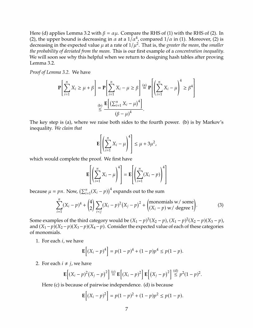
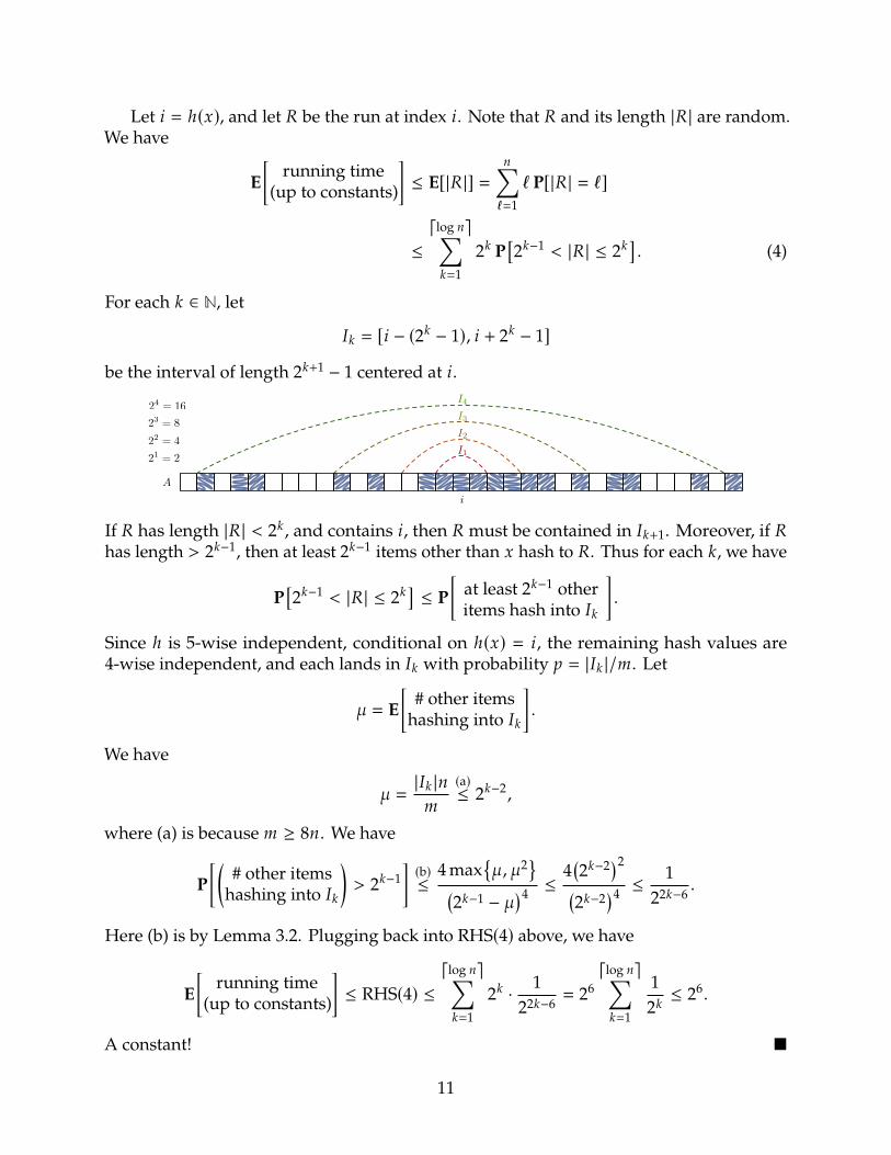
For each : ∈ N, let

�: = [8 − (2: − 1), 8 + 2: − 1]

be the interval of length 2:+1 − 1 centered at 8.

A<latexit sha1_base64="DC/qdQlZgHusAbleDmSKJF3LdWA=">AAACZnicbVHLattAFB0pfThu6yYtpYtuhppCVkZKA0l2Kd10Vwfi2GALMxpf2YPnIWauGozQF2SbfFz/oJ/RkSxC3PTADIdzz33M3DSXwmEU/Q7CvWfPX7zs7HdfvX7Te3tw+O7amcJyGHEjjZ2kzIEUGkYoUMIkt8BUKmGcrr/X8fEvsE4YfYWbHBLFllpkgjP00uW3+UE/GkQN6FMSt6RPWgznh8HP2cLwQoFGLplz0zjKMSmZRcElVN1Z4SBnfM2WMPVUMwUuKZtJK/rFKwuaGeuPRtqojzNKppzbqNQ7FcOV+zdWi/+LTQvMzpJS6LxA0HzbKCskRUPrZ9OFsMBRbjxh3Ao/K+UrZhlH/zk7Xera1mXO16jnbFpx+8SSpkZ6C209tVDG1a5NQoZWLFfodQ033CjF9KKcQe6q5hbS6KpZwXkDuiWnJy05jx9WcH08iL8Oji9P+hdH7TI65BP5TI5ITE7JBflBhmREOAFyS+7IffAn7IUfwo9baxi0Oe/JDkL6F4wKvGg=</latexit>

21 = 2<latexit sha1_base64="ly8gNiDLD0VK0ipf0tpGLVZleZU=">AAACbHicbVFdSxtBFJ2s1aZ+a/smhcGg+BR2U0HzIAh96VsVjBGSKLOTu8mQ+Vhm7iph2R/R1/rL/BP9DZ3dLGJqD8xwOPfcj5kbp1I4DMOXRrDyYXXtY/PT+sbm1vbO7t7+rTOZ5dDjRhp7FzMHUmjooUAJd6kFpmIJ/Xj2vYz3H8E6YfQNzlMYKTbRIhGcoZf6nfuIXtDOw24rbIcV6HsS1aRFalw97DV+DseGZwo0csmcG0RhiqOcWRRcQrE+zBykjM/YBAaeaqbAjfJq3oIeeWVME2P90Ugr9W1GzpRzcxV7p2I4df/GSvF/sUGGyfkoFzrNEDRfNEoySdHQ8vF0LCxwlHNPGLfCz0r5lFnG0X/RUpeytnWJ8zXKOatW3L6zxLGR3kJrTynkUbFsk5CgFZMpel3DEzdKMT3Oh5C6orqFNLqoVtCtQBfk7LQm3eh1BbeddvSt3bk+bV2e1MtokgNySE5IRM7IJflBrkiPcDIjv8hv8tz4E3wJDoKvC2vQqHM+kyUEx38B0b+90w==</latexit>

22 = 4<latexit sha1_base64="2F4cQy3C0Cc6XihBk9CMLL8zPrA=">AAACbHicbVHLSiNBFK20Oj7GGZ87EYoJDq5Cdww4LgYEN7MbB4wRkijVldtJkXo0VbdnCE1/hFv9Mn/Cb7C60wxGPVDF4dxzH1U3TqVwGIZPjWBpeeXT6tr6xufNL1+3tnd2r53JLIcuN9LYm5g5kEJDFwVKuEktMBVL6MXTizLe+wvWCaOvcJbCULGxFongDL3Ua9+26U/audtuhq2wAn1Popo0SY3Lu53G78HI8EyBRi6Zc/0oTHGYM4uCSyg2BpmDlPEpG0PfU80UuGFezVvQI6+MaGKsPxpppb7OyJlybqZi71QMJ+5trBQ/ivUzTH4Mc6HTDEHzeaMkkxQNLR9PR8ICRznzhHEr/KyUT5hlHP0XLXQpa1uXOF+jnLNqxe07Sxwb6S209pRCHhWLNgkJWjGeoNc1/ONGKaZH+QBSV1S3kEYX1QrOKtA5Oe3U5Cz6v4Lrdis6abX/dJrnx/Uy1sgB+UaOSUROyTn5RS5Jl3AyJffkgTw2noP94CA4nFuDRp2zRxYQfH8B18m91g==</latexit>

23 = 8<latexit sha1_base64="lphAQQY3Am+Yi6rlEdV2BGcuCb8=">AAACbHicbVHLSiNBFK20js/x7U6EwqC4Ct1RUBcDght3OjAxQhKlunI7KVKPpuq2Q2j6I9w6XzY/Md8w1Z1mmKgHqjice+6j6sapFA7D8HcjWFj8srS8srq2/nVjc2t7Z/fBmcxy6HAjjX2MmQMpNHRQoITH1AJTsYRuPLkp490XsE4Y/QOnKQwUG2mRCM7QS9320xn9Ri+ft5thK6xAP5KoJk1S4/55p3HXHxqeKdDIJXOuF4UpDnJmUXAJxVo/c5AyPmEj6HmqmQI3yKt5C3rslSFNjPVHI63U/zNyppybqtg7FcOxex8rxc9ivQyTy0EudJohaD5rlGSSoqHl4+lQWOAop54wboWflfIxs4yj/6K5LmVt6xLna5RzVq24/WCJYyO9hdaeUsijYt4mIUErRmP0uoaf3CjF9DDvQ+qK6hbS6KJawVUFOiMX5zW5iv6t4KHdis5a7e/nzevTehkr5IAckVMSkQtyTW7JPekQTibklbyRX40/wX5wEBzOrEGjztkjcwhO/gLh173b</latexit>

24 = 16<latexit sha1_base64="Ivgn8D7yImmCYW4IbV3zGoWSprA=">AAACa3icbVHLThsxFHWGllcp5bFrWViNkFhFM2nEY4GExIZdQWoCUhKQx7mTGPwY2XdA0Wj+gS38GR/BP+CZjKoGeiRbR+ee+7BvnErhMAxfGsHCp8+LS8srq1/Wvq5/29jc6jmTWQ5dbqSxVzFzIIWGLgqUcJVaYCqWcBnfnZbxy3uwThj9B6cpDBUba5EIztBLvfZ15zjav9lohq2wAv1Iopo0SY3zm83G78HI8EyBRi6Zc/0oTHGYM4uCSyhWB5mDlPE7Noa+p5opcMO8Gregu14Z0cRYfzTSSv03I2fKuamKvVMxnLj3sVL8X6yfYXI4zIVOMwTNZ42STFI0tHw7HQkLHOXUE8at8LNSPmGWcfQ/NNelrG1d4nyNcs6qFbcfLHFspLfQ2lMKeVTM2yQkaMV4gl7X8MCNUkyP8gGkrqhuIY0uqhUcVaAzctCpyVH0dwW9div61WpfdJone/UylskP8pPskYgckBNyRs5Jl3BySx7JE3luvAbbwfdgZ2YNGnXONplDsPsGmzy9wQ==</latexit>

i<latexit sha1_base64="pZ11xZQzr/2OULWRn0hd+lzz+MY=">AAACZnicbVHLSgMxFE3H9/uFuHATLIKrMqOCuhPcuFPBqtAWyaR32mAeQ3JHKcN8gVv9OP/AzzAzHcSqBxIO5577SG6cSuEwDD8awdT0zOzc/MLi0vLK6tr6xuadM5nl0OZGGvsQMwdSaGijQAkPqQWmYgn38dNFGb9/BuuE0bc4SqGn2ECLRHCGXroRj+vNsBVWoH9JVJMmqXH9uNG46vYNzxRo5JI514nCFHs5syi4hGKxmzlIGX9iA+h4qpkC18urSQu675U+TYz1RyOt1J8ZOVPOjVTsnYrh0P2OleJ/sU6GyWkvFzrNEDQfN0oySdHQ8tm0LyxwlCNPGLfCz0r5kFnG0X/ORJeytnWJ8zXKOatW3P6xxLGR3kJrTynkUTFpk5CgFYMhel3DCzdKMd3Pu5C6orqFNLqoVnBWgY7JyXFNzqLvFdwdtqKj1uHNcfP8oF7GPNkle+SAROSEnJNLck3ahBMgr+SNvDc+g9VgO9gZW4NGnbNFJhDQL9xavJA=</latexit>

I1<latexit sha1_base64="ryFZKhf8CgspLO6U1zYyD2SIJb8=">AAACaHicbVHLThsxFHWGUiiFEtpFVXVjEVViFY15FLJD6oauSkUDSEkUeZw7iYUfI/tOq2g0n8AWvo1f4CvwTEZqAz2SraNzz33YN8mU9BjHD61o5dXq67X1NxtvN7febbd33l96mzsBfWGVddcJ96CkgT5KVHCdOeA6UXCV3Hyr4le/wXlpzS+cZzDSfGpkKgXHIF18H7NxuxN3j2LW+xrTuBvXqMkJO2CUNUqHNDgf77R+DCdW5BoMCsW9H7A4w1HBHUqhoNwY5h4yLm74FAaBGq7Bj4p61pJ+CcqEptaFY5DW6r8ZBdfez3USnJrjzD+PVeL/YoMc05NRIU2WIxixaJTmiqKl1cPpRDoQqOaBcOFkmJWKGXdcYPiepS5VbedTH2pUc9athHthSRKrgoU2nkooWLlsU5Cik9MZBt3AH2G15mZSDCHzZX1LZU1Zr6BXgy7I8WFDen9XcLnfZQfd/Z+HndO9Zhnr5DPZJXuEkWNySs7IOekTQabkltyR+9Zj1I4+Rp8W1qjV5HwgS4h2nwBLRL02</latexit>

I2<latexit sha1_base64="tekcmZsZ84C2iPz0H6ztrBJWQkU=">AAACaHicbVHLjtMwFHXDaxheHVggxMaaCmlWkdNJNWQ3EhtYMQg6M1JbVY5701rjR2TfgKoon8AWvo1f4Ctw0ghR4Ei2js4992HfvFTSI2M/BtGt23fu3ju4f/jg4aPHT4ZHTy+9rZyAqbDKuuuce1DSwBQlKrguHXCdK7jKb9608avP4Ly05hNuS1hovjaykIJjkD6+W46XwxGLJyzJJhll8XjCsjQNhCWMnaY0iVmHEelxsTwavJ+vrKg0GBSKez9LWImLmjuUQkFzOK88lFzc8DXMAjVcg1/U3awNfRWUFS2sC8cg7dQ/M2quvd/qPDg1x43/O9aK/4vNKixeL2ppygrBiF2jolIULW0fTlfSgUC1DYQLJ8OsVGy44wLD9+x1aWs7X/hQo52zayXcP5Y8typYaO9phTpp9m0KCnRyvcGgG/girNbcrOo5lL7pbqmsaboVZB3ojpylPcmS3yu4HMfJaTz+kI7OT/plHJCX5JickISckXPyllyQKRFkTb6Sb+T74Gc0jJ5HL3bWaNDnPCN7iI5/AYHyvVI=</latexit>

I3<latexit sha1_base64="wArUR9zXMXhg76lzZKGETM0dzOA=">AAACaHicbVHLThsxFHWmLwptCbCoqm4sIiRW0UweDdkhsaGrUpUAUhJFHudOYuHHyL7TKhrNJ3QL38Yv8BV4JqOKtD2SraNzz33YN06lcBiGD43gxctXr99svd3eeff+w25zb//KmcxyGHEjjb2JmQMpNIxQoISb1AJTsYTr+PasjF//BOuE0Ze4SmGq2EKLRHCGXvrxddadNVthux9Gw/6Qrkk39CSMeoP+Fxq1wwotUuNittf4NpkbninQyCVzbhyFKU5zZlFwCcX2JHOQMn7LFjD2VDMFbppXsxb0yCtzmhjrj0Zaqc8zcqacW6nYOxXDpfs7Vor/i40zTE6mudBphqD5ulGSSYqGlg+nc2GBo1x5wrgVflbKl8wyjv57NrqUta1LnK9Rzlm14vYfSxwb6S209pRCHhWbNgkJWrFYotc1/OJGKabn+QRSV1S3kEYX1QqGFeiaDHo1GUZ/VnDVaUfddud7r3V6XC9ji3wmh+SYRGRATsk5uSAjwsmC/CZ35L7xGDSDj8GntTVo1DkHZAPB4ROU5L1c</latexit>

I4<latexit sha1_base64="Tu8yPoCrCrEGqTneITrH1PwL/+4=">AAACaHicbVHLbhMxFHWGVymvFBYIsbEaIXUVedKUZHaV2JQVRZC2UhJFHudOYtWPkX0HFI3mE9jCt/UX+hX1TEaIAEeydXTuuQ/7prmSHhm76UT37j94+Gjv8f6Tp8+ev+gevLzwtnACJsIq665S7kFJAxOUqOAqd8B1quAyvf5Qxy+/gfPSmq+4yWGu+crITAqOQfrycTFcdHusPzhhyWhMWf+ExclwEAhj4+Q9o3EgNXqkxfnioPNptrSi0GBQKO79NGY5zkvuUAoF1f6s8JBzcc1XMA3UcA1+XjazVvRdUJY0sy4cg7RR/8woufZ+o9Pg1BzX/u9YLf4vNi0wG89LafICwYhto6xQFC2tH06X0oFAtQmECyfDrFSsueMCw/fsdKlrO5/5UKOes2kl3D+WNLUqWGjrqYUyrnZtCjJ0crXGoBv4LqzW3CzLGeS+am6prKmaFSQN6JaMhi1J4t8ruBj04+P+4POwd3rULmOPvCWH5IjEZEROyRk5JxMiyIr8ID/Jr85t1I1eR2+21qjT5rwiO4gO7wCgsL1i</latexit>

If ' has length |' | < 2:, and contains 8, then ' must be contained in �:+1. Moreover, if '

has length > 2:−1

, then at least 2:−1

items other than G hash to '. Thus for each :, we have

P[2:−1 < |' | ≤ 2

:]≤ P

[at least 2

:−1other

items hash into �:

].

Since ℎ is 5-wise independent, conditional on ℎ(G) = 8, the remaining hash values are

4-wise independent, and each lands in �: with probability ? = |�: |/<. Let

� = E[# other items

hashing into �:

].

We have

� =|�: |=<

(a)≤ 2

:−2,

where (a) is because < ≥ 8=. We have

P[(

# other items

hashing into �:

)> 2

:−1

](b)≤

4 max

{�, �2

}(2:−1 − �

)4

≤4

(2:−2

)2(

2:−2

)4

≤ 1

22:−6

.

Here (b) is by Lemma 3.2. Plugging back into RHS(4) above, we have

E[

running time

(up to constants)

]≤ RHS(4) ≤

dlog =e∑:=1

2: · 1

22:−6

= 26

dlog =e∑:=1

1

2:≤ 2

6.

A constant! �

11

5 Takeaways• Dictionary data structures provide everyday motivation for studying randomization,

where hash tables offer simpler and better performance (in expectation) than search

trees.

• There are different ways to implement hash tables and they mostly differ in how they

handle collisions.

• Chaining uses linked lists to handle collisions. It has reasonable performance inexpectation for universal hash functions, and stronger guarantees when the hash

function is more independent.

• Linear probing is perhaps the easiest hash table to implement, and is also the most

hardware friendly. It had been observed to perform well in practice long before it

had been properly analyzed.

• The analysis of linear probing cleverly uses canonical intervals (doubling in size) to

limit the number of “bad events” we have to avoid, to roughly log = (per key).

• It turns out that 5-wise independence is sufficient for linear probing to have $(1)running time in expectation. Interestingly, 4-wise independence is not enough.

6 ExercisesExercise 1. Let ℎ : [=] → [ℓ ] be a hash function, with ℓ ≥ =.

1. Suppose ℎ is an ideal hash function. What is the exact probability that ℎ has no

collisions (i.e., ℎ is injective)?

2. Suppose ℎ is a universal hash function. Show that for ℓ ≥ =2, ℎ has no collisions with

probability ≥ 1/2 − 1/2=.

Exercise 2. Consider the particular case of hash tables with chaining with : = 2= and an

ideal hash function ℎ : [=] → [:].

1. Consider a particular array slot �[8]. Show that the probability that �[8] has ≥ ℓitems hashed to it is

P[at least ℓ items being hashed to �[8]

]≤ 1

ℓ ! 2ℓ.

2. Show that, with probability of error ≤ 1/=2, the maximum length is at most $

(log =

).

3. Show that, with probability of error ≤ 1/=2, the maximum length is at most

$(log(=)/log log =

)(maybe with a slightly higher hidden constant than in part

2).

12

Exercise 3. The goal of this exercise is to show how to get constant time access for = keys

with $(=) space, using only universal hash functions.

We first allocate an array �[1..=] of size =. We have one universal hash function ℎ0 into

[=]. If we have a set of (say) : collisions at an array cell �[8], rather than making a linked

list of length :, and we build another hash table, with a new universal hash function ℎ8 , of

size :2, with no collisions (per Exercise 1). (We may have to retry if there is a collision.) If

the total size (summing the lengths of the first arrray and each of the second arrays) comes

out to bigger than (say) 5=, we try again.

1. For each 8 = 1, . . . , =, let :8 be the number of keys that hash to the 8th cell. We have(sum of array sizes of our data structure

)≤ = +

=∑8=1

:2

8 .

Show that

=∑8=1

:2

8 ≤(total # of ordered pairs of colliding keys in ℎ0

).

(Here an ordered pair is defined by a coordinate pair (8 , 9), where 8 , 9 ∈ [=] and are

allowed to be equal.)

2. Show that

E[total # of ordered pairs of colliding keys

]≤ 2=.

3. Show that

P[ (sum of all array sizes

)> 5=

]< 1/2.

Taken together, steps 1 to 3 above show that this approach will build a “perfect”

hash table over the = keys in $(=) space with probability of success at least 1/2, usingonly universal hash functions. Even if it fails to work, we can then keep repeating the

construction until it succeeds. Note that, due to the reliance on resampling, this approach

works better in static settings, when the set of keys is fixed.

Exercise 4. Prove Theorem 3.3.

References[1] David R. Karger, Eric Lehman, Frank Thomson Leighton, Rina Panigrahy, Matthew S.

Levine, and Daniel Lewin. “Consistent Hashing and Random Trees: Distributed

Caching Protocols for Relieving Hot Spots on the World Wide Web”. In: Proceedingsof the Twenty-Ninth Annual ACM Symposium on the Theory of Computing, El Paso, Texas,USA, May 4-6, 1997. Ed. by Frank Thomson Leighton and Peter W. Shor. ACM, 1997,

pp. 654–663.

13

[2] Donald Knuth. Notes on “open” addressing. 1963. url: http://jeffe.cs.illinois.edu/

teaching/datastructures/2011/notes/knuth-OALP.pdf.

[3] Donald R. Morrison. “PATRICIA—Practical Algorithm To Retrieve Information

Coded in Alphanumeric”. In: J. ACM 15.4 (Oct. 1968), 514–534.

[4] Jelani Nelson. Load balancing, :-wise independence, chaining, linear probing. Recordedlecture. 2016. url: https://www.youtube.com/watch?v=WqBc0ZCU4Uw.

[5] Anna Pagh, Rasmus Pagh, and Milan Ruzic. “Linear Probing with Constant In-

dependence”. In: SIAM J. Comput. 39.3 (2009). Preliminary version in STOC, 2007,

pp. 1107–1120.

[6] Mihai Patrascu and Mikkel Thorup. “On the k-Independence Required by Lin-

ear Probing and Minwise Independence”. In: ACM Trans. Algorithms 12.1 (2016).

Preliminary version in ICALP, 2010, 8:1–8:27.

[7] Jeanette P. Schmidt and Alan Siegel. “On Aspects of Universality and Performance

for Closed Hashing (Extended Abstract)”. In: Proceedings of the 21st Annual ACMSymposium on Theory of Computing, May 14-17, 1989, Seattle, Washigton, USA. Ed. byDavid S. Johnson. ACM, 1989, pp. 355–366.

[8] Jeanette P. Schmidt and Alan Siegel. “The Analysis of Closed Hashing under Limited

Randomness (Extended Abstract)”. In: Proceedings of the 22nd Annual ACM Symposiumon Theory of Computing, May 13-17, 1990, Baltimore, Maryland, USA. Ed. by Harriet

Ortiz. ACM, 1990, pp. 224–234.

[9] Daniel Dominic Sleator and Robert Endre Tarjan. “Self-Adjusting Binary Search

Trees”. In: J. ACM 32.3 (1985), pp. 652–686. Preliminary version in STOC, 1983.

[10] Mikkel Thorup. “LinearProbingwith 5-IndependentHashing”. In:CoRR abs/1509.04549

(2015). arXiv: 1509.04549. url: http://arxiv.org/abs/1509.04549.

14