Linear Programming
65
11 Linear Programming LEARNING OBJECTIVES : After studying this unit you will be able to : l Formulate a problem in LP l Understand the circumstances in which LP technique can be used l Calculate marginal rates of substitution and opportunity cost using the graphic method l Construct the initial tableau using the Simplex Method l Explain the meaning odf entries in each column of final tableau l Describe hoe technique of Linear Programming can be used in decision making, planning and control 11.1 INTRODUCTION Linear programming is a mathematical technique for determining the optimal allocation of re- sources and achieving the specified objective when there are alternative uses of the resources like money, manpower, materials, machines and other facilities. The objective in resource allo- cation may be either cost minimization or profit maximization. The technique of linear program- ming is applicable to all problems in which the total effectiveness about the use of resources can be expressed as a linear function of individual allocations, and the limitations on resources give rise to linear equalities or inequalities of individual allocations. The adjective linear, is to be particularly noted here. It implies that all the limitations or constraints and the objective must be expressed as linear functions. Although the technique of linear programming is applicable to all such problems, there are some more easy methods for solving specific categories of problems. Special algorithms have been evolved to ease up computational task. The algorithms have acquired special names of their own. This has led to the following categories of the linear programming problems : (i) General Linear Programming Problems. (ii) Transportation Problems. (iii) Assignment Problems.
-
Upload
khangminh22 -
Category
Documents
-
view
2 -
download
0
Transcript of Linear Programming
11Linear Programming
LEARNING OBJECTIVES :
After studying this unit you will be able to :
� Formulate a problem in LP
� Understand the circumstances in which LP technique can be used
� Calculate marginal rates of substitution and opportunity cost using the graphic method
� Construct the initial tableau using the Simplex Method
� Explain the meaning odf entries in each column of final tableau
� Describe hoe technique of Linear Programming can be used in decision making,planning and control
11.1 INTRODUCTION
Linear programming is a mathematical technique for determining the optimal allocation of re-sources and achieving the specified objective when there are alternative uses of the resourceslike money, manpower, materials, machines and other facilities. The objective in resource allo-cation may be either cost minimization or profit maximization. The technique of linear program-ming is applicable to all problems in which the total effectiveness about the use of resources canbe expressed as a linear function of individual allocations, and the limitations on resources giverise to linear equalities or inequalities of individual allocations. The adjective linear, is to beparticularly noted here. It implies that all the limitations or constraints and the objective must beexpressed as linear functions.
Although the technique of linear programming is applicable to all such problems, there are somemore easy methods for solving specific categories of problems. Special algorithms have beenevolved to ease up computational task. The algorithms have acquired special names of theirown. This has led to the following categories of the linear programming problems :
(i) General Linear Programming Problems.
(ii) Transportation Problems.
(iii) Assignment Problems.
11.2 Advanced Management Accounting
We know that there is an opportunity cost for scarce resources that should be included in therelevant cost calculation for decision making and variance calculations. In practice severalresources may be scarce. The opportunity cost of these scarce resources can be determined bythe use of linear programming techniques. Our objective in this chapter is to examine linearprogramming techniques and to consider how they can be applied to some specific types ofdecisions that a firm may have to make.
11.1.1 General Linear Programming Problems :An examination of the following simple exampleshould illustrate the basic concepts of linear programming problem (abbreviated as LPP).
Illustration
A small scale industry unit manufactures two products, X1 and X
2 which are processed in the
machine shop and the assembly shop. The time (in hours) required for each product in theshops are given in the matrix below. Profit per unit is also given along.
Machine shop Assembly shop Profit per unit
Product X1
2 hours 4 hours Rs. 3
Product X2
3 hours 2 hours Rs. 4
Total time available (hours) 16 16
(in a day)
Assuring that there is unlimited demand for both products how many units of each should beproduced every day to maximize total profit ?
Let x1 and x
2 be the number of units of X
1 and X
2 respectively that maximize the profit.
To begin solving the problem, let us restate the information in mathematical form. To do so, weintroduce a term "objective function". This refers to the expression which shows the relationshipof output to profit.
3x1 = total daily profit from the sale of x
1 units
product X
1
4x2 = total daily profit from the sale of x
2 units product X
2
Objective function Max Profit = 3x1 + 4x2
Department time constraints
Time used in making x1 and x
2 units of two products must not exceed the total daily time
available in two shops. In other words, (the hours required to make 1 unit of product X1)
multiplied by (the number of units of product X1) plus ( the hours required to make 1 unit of
product X2) multiplied by (the number of units of product X
2) must be less than or equal to
the daily time available in each shop. Mathematically it is stated as
2x1 + 3x
2 ≤ 16 Machine shop constraint
4x1 + 2x
2 ≤ 16 Assembles shop constraint
In order to obtain meaningful answers, the values calculated for x1 and x2 cannot be negatives;they must represent real product X1 and product X2. Thus, all elements of the solution to theformulated linear programming problem must be either greater than or equal to 0 (x1 > 0, x2 > 0).The machine and assembly shops contraints are called structural constraints.

11.3Linear Programming
The problem can be summarized in a mathematical form as below :
Maximize:
Profit = 3x1 + 4 x
2
Subject to the constraints
2x1 + 3 x
2 ≤ 16
4x1 + 2x
2 ≤ 16
x1 ≥ 0, x
2 > 0.
M ethod of L inear Program m ing
G raphica l M ethod S im plex M ethod
11.2 GRAPHICAL METHOD
The graphical method discussed here provides necessary grounding in understanding thecomputational steps of the simplex algorithms, it itself being of little use in handling practicalproblems. It is possible to solve conveniently linear programming problems graphically as longas the number of variables (products, for example) are not more than two. Before we proceed toexplain the graphical method, let us first know how linear inequalities are handled graphically.
11.2.1 Linear inequalities in one variable and the solution space
Any relation or function of degree one that involves an inequality sign is a linear inequality. It maybe of one variable, or, may be of more than one variable. Simple examples of linear inequalitiesare those of one variable only; viz. x > 0, x < 0, etc.
x > 0 x < 0
-3 -2 -1 0 1 2 3 -3 -2 -1 0 1 2 3
The values of the variables that satisfy an inequality are called the solution space, and is abbre-viated as S.S. The solution spaces for (i) x > 0, (ii) x < 0 are shown by the dark portion in theabove diagrams.
11.2.2 Linear inequalities in two variables : Now we turn to linear inequalities in two variablesx, and y, and shade a few S.S.
x>0 x ≥ 0
x>0y >0
x ≥ 0y ≥ 0
x
yyy
xx
y
x
11.4 Advanced Management Accounting
Note : The pair of inequalities x ³ 0, y ³ 0 playan important role in linear programmingproblems.
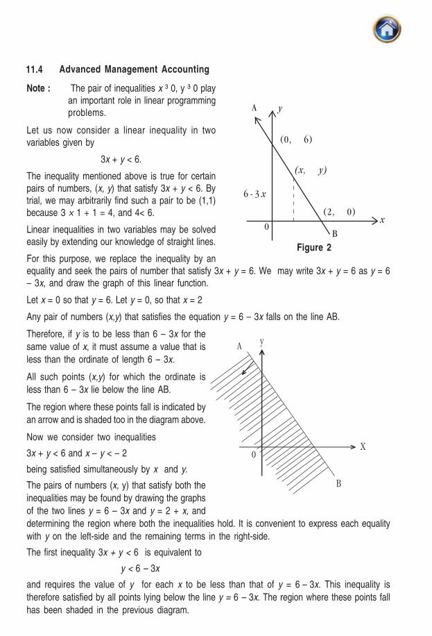
Let us now consider a linear inequality in twovariables given by
3x + y < 6.
The inequality mentioned above is true for certainpairs of numbers, (x, y) that satisfy 3x + y < 6. Bytrial, we may arbitrarily find such a pair to be (1,1)because 3 × 1 + 1 = 4, and 4< 6.
Linear inequalities in two variables may be solvedeasily by extending our knowledge of straight lines.
For this purpose, we replace the inequality by anequality and seek the pairs of number that satisfy 3x + y = 6. We may write 3x + y = 6 as y = 6– 3x, and draw the graph of this linear function.
Let x = 0 so that y = 6. Let y = 0, so that x = 2
Any pair of numbers (x,y) that satisfies the equation y = 6 – 3x falls on the line AB.
Therefore, if y is to be less than 6 – 3x for the
same value of x, it must assume a value that is
less than the ordinate of length 6 – 3x.
All such points (x,y) for which the ordinate is
less than 6 – 3x lie below the line AB.
The region where these points fall is indicated by
an arrow and is shaded too in the diagram above.
Now we consider two inequalities
3x + y < 6 and x – y < – 2
being satisfied simultaneously by x and y.
The pairs of numbers (x, y) that satisfy both the
inequalities may be found by drawing the graphs
of the two lines y = 6 – 3x and y = 2 + x, and
determining the region where both the inequalities hold. It is convenient to express each equality
with y on the left-side and the remaining terms in the right-side.
The first inequality 3x + y < 6 is equivalent to
y < 6 – 3x
and requires the value of y for each x to be less than that of y = 6 – 3x. This inequality is
therefore satisfied by all points lying below the line y = 6 – 3x. The region where these points fall
has been shaded in the previous diagram.
x0
B
(2, 0)
Figure 2
6 - 3 x
yA
(0, 6)
(x, y)
A
0
y
X
B

11.5Linear Programming
y
x
yA
C
BD
yy = + 2 x
x(0 ,2 )
(-2 ,0)
0
We consider the second inequality x – y < – 2, and note that this is equivalent to y > 2 + x.
It requires the value of y for each x to be larger than that of y = 2 + x. This inequality is, therefore,
satisfied by all points lying above the line y = 2 + x.
The region is indicated by an arrow on the line y = 2 + x
For x = 0, y = 2 + 0 = 2. For y = 0, 0 = 2 + x \ x = – 2.
By superimposing the above two graphs we determine the common region ACD in which thepairs (x,y) satisfy both the inequalities.
Note : [1] The inequalities 3x + y < 6 and x - y < 2 differ from the preceding ones in that these also
include equality signs. It means that the points lying on the corresponding lines are also included
in the region.
[2] The procedure may be extended to any number of inequalities.
11.2.3 Graphical solution for linear programming problem : We consider the problem of
maximizing a linear function Z = x + 2 y subject to the restrictions
x > 0, y > 0, x < 6, y < 7, x + y < 12
11.6 Advanced Management Accounting
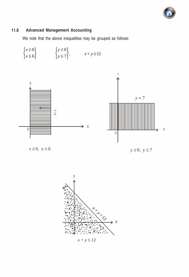
We note that the above inequalities may be grouped as follows:
⎭⎬⎫
⎩⎨⎧
≤≥
6
0
x
x
⎭⎬⎫
⎩⎨⎧
≤≥
7
0
y
y, x+ y ≤ ⋅12
y
��
9=x
X
y
�
y ≥ 0, y ≤ 7x ≥ 0, x ≤ 6
y
XO
x +y =
12
x + y ≤ 12
y = 7
11.7Linear Programming
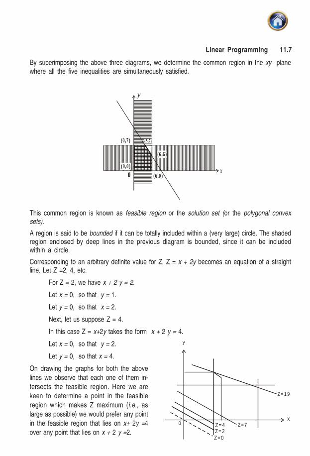
By superimposing the above three diagrams, we determine the common region in the xy planewhere all the five inequalities are simultaneously satisfied.
This common region is known as feasible region or the solution set (or the polygonal convexsets).
A region is said to be bounded if it can be totally included within a (very large) circle. The shadedregion enclosed by deep lines in the previous diagram is bounded, since it can be includedwithin a circle.
Corresponding to an arbitrary definite value for Z, Z = x + 2y becomes an equation of a straightline. Let Z =2, 4, etc.
For Z = 2, we have x + 2 y = 2.
Let x = 0, so that y = 1.
Let y = 0, so that x = 2.
Next, let us suppose Z = 4.
In this case Z = x+2y takes the form x + 2 y = 4.
Let x = 0, so that y = 2.
Let y = 0, so that x = 4.
On drawing the graphs for both the above
lines we observe that each one of them in-
tersects the feasible region. Here we are
keen to determine a point in the feasible
region which makes Z maximum (i.e., as
large as possible) we would prefer any point
in the feasible region that lies on x+ 2y =4
over any point that lies on x + 2 y =2.
y
0
Z=0Z=2Z=4 Z= 7
Z= 1 9
X
x
(0 ,7 )
0 (6 ,0 )
(6 ,6 )
(0 ,0 )
y
11.8 Advanced Management Accounting
Following the same reasoning we find that we can get point in the feasible region for
which Z is maximum. The maximum value for Z is achieved when the line x + 2 y = Z is moved
parallel to itself upward as far as possible subject to the restriction that it must intersect the
feasible region (shown by the deep line in the diagram on previous page). This is seen to occur
when it passes through the point (5,7) the point of intersection of x + y = 12 and y = 5. It is noted
that this point (5,7) is one of the corner points (or extreme points) of the solution set.
We may similarly find the point in the feasible region for which Z is minimum. It is found to occur
at (0,0) which is again a corner point of the solution set but situated opposite to the point for
which Z is maximum. The values of x and y so determined constitutes the solution to the
problem.
Thus the objective function attains a maximum or a minimum value at one of the corner
points of the feasible solution known as extreme points of the solution set. Once these
extreme points (the points of intersection of lines bounding the region) are known, a compact matrix
representation of these points is possible. We shall denote the matrix of the extreme points by E.
The coefficients of the objective function may also be represented by a column vector. We shall
represent this column vector by C.
The elements in the product matrix EC shows different values, which the objective function
attains at the various extreme points. The largest and the smallest elements in matrix EC are
respectively the maximum and the minimum values of the objective function. The row in matrix
EC in which this happens is noted and the elements in that row indicate the appropriate pairing
and is known as the optimal solution.
In the context of the problem under consideration.
x y
E =
⎟⎟⎟⎟⎟⎟
⎠
⎞
⎜⎜⎜⎜⎜⎜
⎝
⎛
66
06
75
70
00
, C = ⎥⎦
⎤⎢⎣
⎡2
1
EC =
⎟⎟⎟⎟⎟⎟
⎠
⎞
⎜⎜⎜⎜⎜⎜
⎝
⎛
66
06
75
70
00
⎥⎦
⎤⎢⎣
⎡2
1 =
⎟⎟⎟⎟⎟⎟
⎠
⎞
⎜⎜⎜⎜⎜⎜
⎝
⎛
×+××+××+××+××+×
2616
2016
2715
2710
2010
=
⎟⎟⎟⎟⎟⎟
⎠
⎞
⎜⎜⎜⎜⎜⎜
⎝
⎛
18
6
19
14
0
The given objective function viz. Z = x + 2y is maximum at the points (5, 7) present in the third rowof the matrix E. Thus the optimal solution is x = 5, y = 7, and the maximum value of the objectivefunction is 19.
x
y
x
y
11.9Linear Programming
We now list the steps to be followed under graphical solution to a linear programming problem.
Step1. Determine the region that satisfies the set of given inequalities.
Step 2. Ensure that the region is bounded*. If the region is not bounded, either there areadditional hidden conditions which can be used to bound the region or there is nosolution to the problem.
Step 3. Construct the matrix E of the extreme points, and the column vector C of the objectivefunction.
Step 4. Find the matrix product EC. For maximization, determine the row in EC where thelargest element appears; while for minimization, determine the row in EC where thesmallest element appears.
Step 5. The objective function is optimized corresponding to the same row elements of theextreme point matrix E.
Note : If the slope of the objective function be same as that of one side of feasible region,there are multiple solutions to the problem. However, the optimized value of theobjective function remains the same.
11.2.4 Application of Graphical Method
Illustration
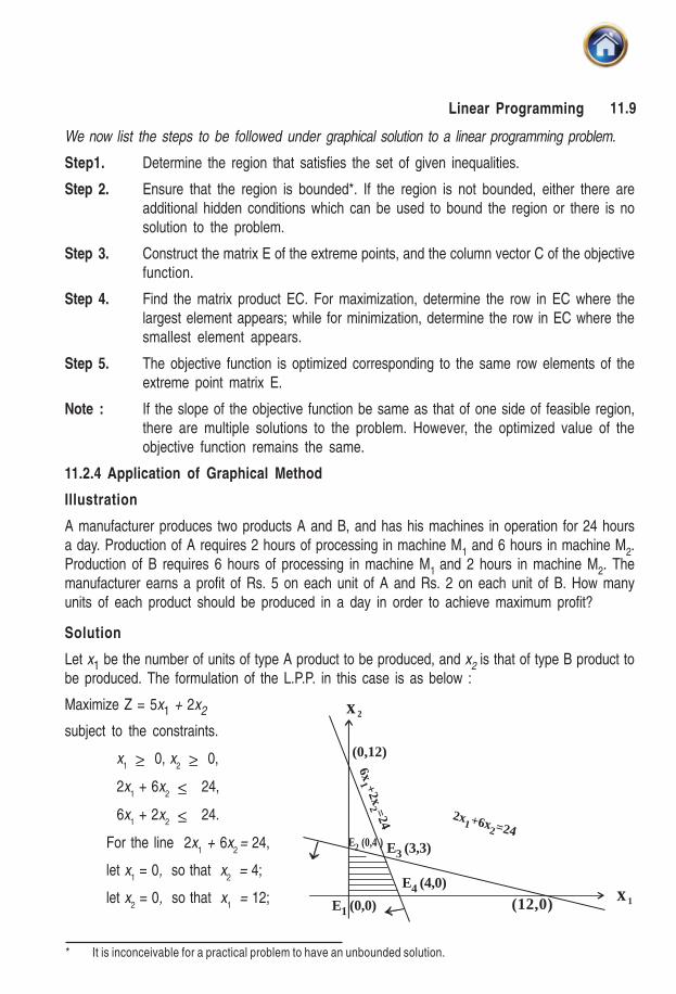
A manufacturer produces two products A and B, and has his machines in operation for 24 hoursa day. Production of A requires 2 hours of processing in machine M1 and 6 hours in machine M2.Production of B requires 6 hours of processing in machine M1 and 2 hours in machine M2. Themanufacturer earns a profit of Rs. 5 on each unit of A and Rs. 2 on each unit of B. How manyunits of each product should be produced in a day in order to achieve maximum profit?
Solution
Let x1 be the number of units of type A product to be produced, and x2 is that of type B product tobe produced. The formulation of the L.P.P. in this case is as below :
Maximize Z = 5x1 + 2x2
subject to the constraints.
x1 ≥ 0, x
2 ≥ 0,
2x1 + 6x
2 ≤ 24,
6x1 + 2x
2 ≤ 24.
For the line 2x1 + 6x
2= 24,
let x1 = 0, so that x
2 = 4;
let x2 = 0, so that x
1 = 12;
* It is inconceivable for a practical problem to have an unbounded solution.
x 1
x 2
(12,0)E1 (0,0)
E4 (4,0)
E3 (3,3)
(0,12)
6x1 +2x
2 =24 2x1+6x2=24E2 (0,4 )
11.10 Advanced Management Accounting
For the line 6x1 + 2x
2 = 24;
let x1 = 0, so that x
2 = 12;
let x2 = 0, so that x
1 = 4.
The shaded portion in the diagram is the feasible region and the matrix of the extreme points E1,E2, E3 and E4 is
x1 x
2
E =
4
3
2
1
E
E
E
E
0
3
4
0
4
3
0
0
⎟⎟⎟⎟⎟
⎠
⎞
⎜⎜⎜⎜⎜
⎝
⎛
The column vector for the objective function is C = 2
1
2
5
x
x⎥⎦
⎤⎢⎣
⎡
The column vector the values of the objective function is given by
EC = ⎟⎟⎟⎟⎟
⎠
⎞
⎜⎜⎜⎜⎜
⎝
⎛
04
33
40
00
⎥⎦
⎤⎢⎣
⎡2
5 =
⎟⎟⎟⎟⎟
⎠
⎞
⎜⎜⎜⎜⎜
⎝
⎛
×+××+××+××+×
2054
2353
2450
2050
=
4
3
2
1
E
E
E
E
20
21
8
0
⎟⎟⎟⎟⎟
⎠
⎞
⎜⎜⎜⎜⎜
⎝
⎛
Since 21 is the largest element in matrix EC, therefore the maximum value is reached at theextreme point E3 whose coordinates are (3,3).
Thus, to achieve maximum profit the manufacturer should produce 3 units each of both theproducts A and B.
Illustration
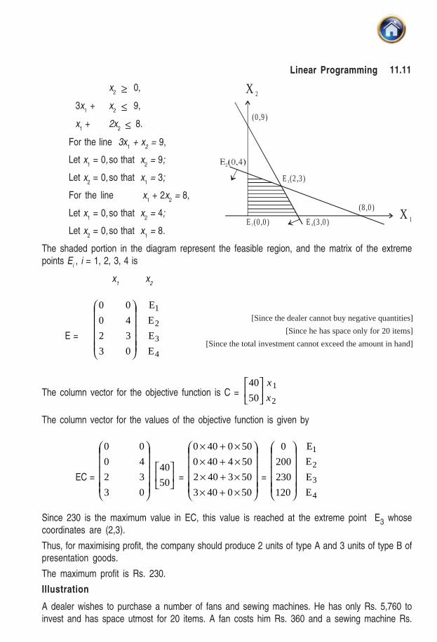
A company produces two types of presentation goods A and B that require gold and silver. Eachunit of type A requires 3 gms. of silver and 1 gm. of gold while that of B requires 1 gm. of silver and2 gms. of gold. The company can procure 9 gms of silver and 8 gms. of gold. If each unit of typeA brings a profit of Rs. 40 and that of types B Rs. 50, determine the number of units of each typethat the company should produce to maximize the profit. What is the maximum profit?
Solution
Let x1 be the number of units of type A of presentation goods to be produced and x2 is that of typeB. The formulation of L.P.P. based on the given data may be stated as follows:
Maximize Z = 40 x1 + 50 x2
Subject to the constraints
x1 ≥ 0,
11.11Linear Programming
x2 ≥ 0,
3x1 + x
2 ≤ 9,
x1 + 2x
2 ≤ 8.
For the line 3x1 + x
2 = 9,
Let x1 = 0,so that x
2 = 9;
Let x2 = 0,so that x
1 = 3;
For the line x1 + 2x
2 = 8,
Let x1 = 0,so that x
2 = 4;
Let x2 = 0,so that x
1 = 8.
The shaded portion in the diagram represent the feasible region, and the matrix of the extremepoints E
i , i = 1, 2, 3, 4 is
x1
x2
E =
4
3
2
1
E
E
E
E
0
3
4
0
3
2
0
0
⎟⎟⎟⎟⎟
⎠
⎞
⎜⎜⎜⎜⎜
⎝
⎛
The column vector for the objective function is C = 2
1
50
40
x
x⎥⎦
⎤⎢⎣
⎡
The column vector for the values of the objective function is given by
EC = ⎟⎟⎟⎟⎟
⎠
⎞
⎜⎜⎜⎜⎜
⎝
⎛
0
3
4
0
3
2
0
0
⎥⎦
⎤⎢⎣
⎡50
40 =
⎟⎟⎟⎟⎟
⎠
⎞
⎜⎜⎜⎜⎜
⎝
⎛
×+××+××+××+×
500403
503402
504400
500400
=
4
3
2
1
E
E
E
E
120
230
200
0
⎟⎟⎟⎟⎟
⎠
⎞
⎜⎜⎜⎜⎜
⎝
⎛
Since 230 is the maximum value in EC, this value is reached at the extreme point E3 whosecoordinates are (2,3).
Thus, for maximising profit, the company should produce 2 units of type A and 3 units of type B ofpresentation goods.
The maximum profit is Rs. 230.
Illustration
A dealer wishes to purchase a number of fans and sewing machines. He has only Rs. 5,760 toinvest and has space utmost for 20 items. A fan costs him Rs. 360 and a sewing machine Rs.
[Since the dealer cannot buy negative quantities]
[Since he has space only for 20 items]
[Since the total investment cannot exceed the amount in hand]
E (0 ,0 )1
(8 ,0 )
E (2 ,3 )3
(0 ,9 )
X 2
X 1E (3 ,0 )4
11.12 Advanced Management Accounting
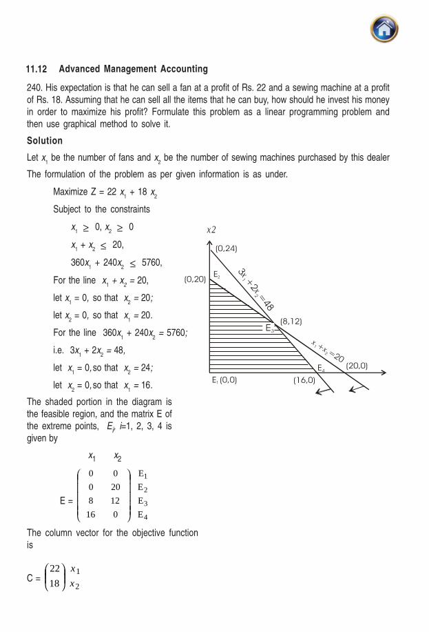
240. His expectation is that he can sell a fan at a profit of Rs. 22 and a sewing machine at a profitof Rs. 18. Assuming that he can sell all the items that he can buy, how should he invest his moneyin order to maximize his profit? Formulate this problem as a linear programming problem andthen use graphical method to solve it.
Solution
Let x1 be the number of fans and x
2 be the number of sewing machines purchased by this dealer
The formulation of the problem as per given information is as under.
Maximize Z = 22 x1 + 18 x
2
Subject to the constraints
x1 ≥ 0, x
2 ≥ 0
x1 + x
2 ≤ 20,
360x1 + 240x
2 ≤ 5760,
For the line x1 + x
2 = 20,
let x1 = 0, so that x
2 = 20;
let x2 = 0, so that x
1 = 20.
For the line 360x1 + 240x
2 = 5760;
i.e. 3x1 + 2x
2 = 48,
let x1 = 0,so that x
2 = 24;
let x2 = 0,so that x
1 = 16.
The shaded portion in the diagram isthe feasible region, and the matrix E ofthe extreme points, Ei, i=1, 2, 3, 4 isgiven by
x1 x2
E =
4
3
2
1
E
E
E
E
0
12
20
0
16
8
0
0
⎟⎟⎟⎟⎟
⎠
⎞
⎜⎜⎜⎜⎜
⎝
⎛
The column vector for the objective functionis
C = 2
1
18
22
x
x⎟⎟⎠
⎞⎜⎜⎝
⎛
x2
������
��������
����
���
���
xx
�
�
xx�
�
����
� ������� � ���
��
������
11.13Linear Programming
The column vector for the values of the objective function is given by
EC = ⎟⎟⎟⎟⎟
⎠
⎞
⎜⎜⎜⎜⎜
⎝
⎛
⎟⎟⎟⎟⎟
⎠
⎞
⎜⎜⎜⎜⎜
⎝
⎛
18
22
0
12
20
0
16
8
0
0
= ⎟⎟⎟⎟⎟
⎠
⎞
⎜⎜⎜⎜⎜
⎝
⎛
×+××+××+×
×+×
1802216
1812228
1820220
180220
=
4
3
2
1
E
E
E
E
352
392
360
0
⎟⎟⎟⎟⎟
⎠
⎞
⎜⎜⎜⎜⎜
⎝
⎛
Since 392 is the largest element of matrix EC, therefore the maximum profit is reached at theextreme point E3 whose coordinates are (8,12). Thus, to maximize his profit the dealer shouldbuy 8 fans and 12 sewing machines.
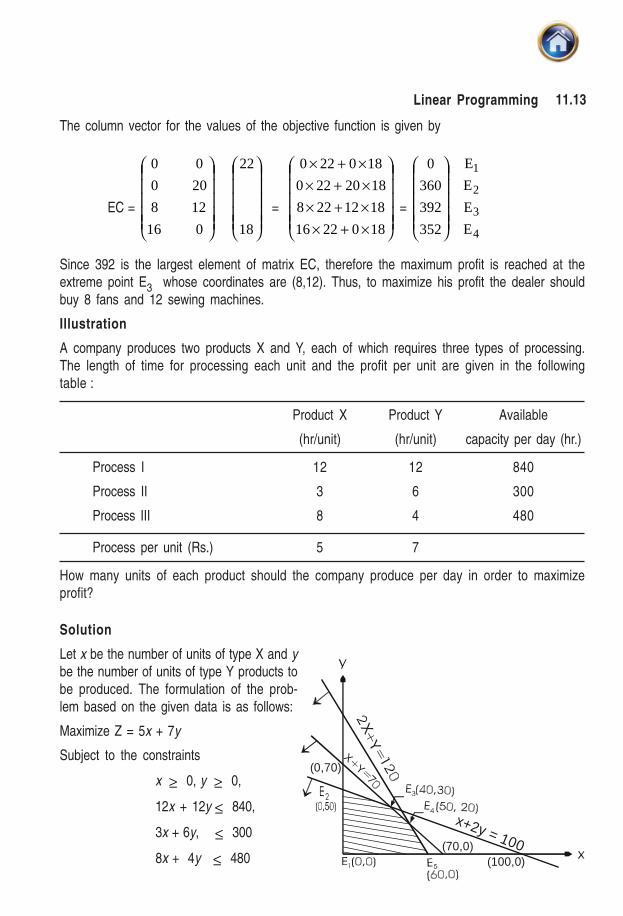
Illustration
A company produces two products X and Y, each of which requires three types of processing.The length of time for processing each unit and the profit per unit are given in the followingtable :
Product X Product Y Available
(hr/unit) (hr/unit) capacity per day (hr.)
Process I 12 12 840
Process II 3 6 300
Process III 8 4 480
Process per unit (Rs.) 5 7
How many units of each product should the company produce per day in order to maximizeprofit?
Solution
Let x be the number of units of type X and ybe the number of units of type Y products tobe produced. The formulation of the prob-lem based on the given data is as follows:
Maximize Z = 5x + 7y
Subject to the constraints
x ≥ 0, y ≥ 0,
12x + 12y ≤ 840,
3x + 6y, ≤ 300
8x + 4y ≤ 480
XY
XY
x+2y = 100
(0,70)
(70,0)(100,0)
11.14 Advanced Management Accounting
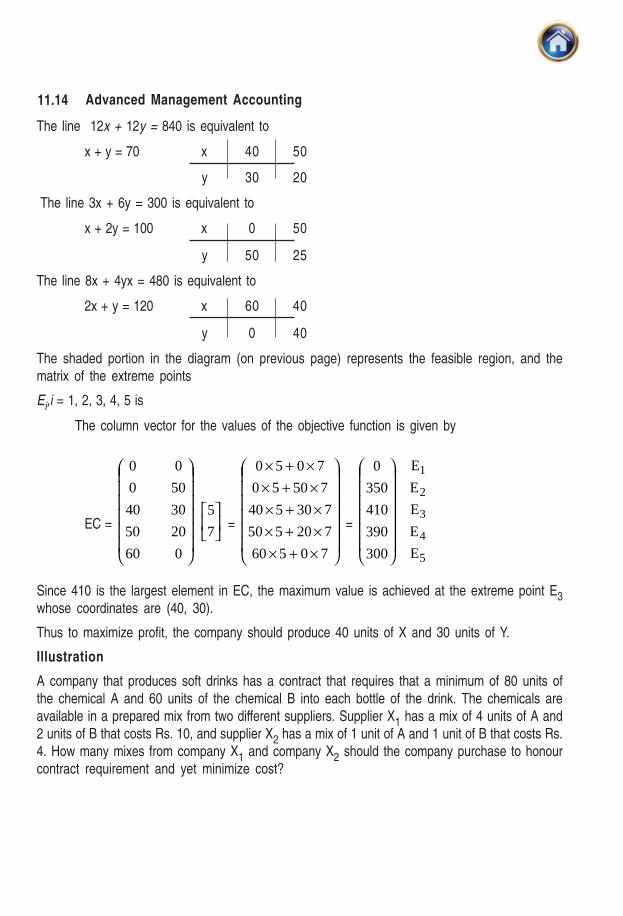
The line 12x + 12y = 840 is equivalent to
x + y = 70 x 40 50
y 30 20
The line 3x + 6y = 300 is equivalent to
x + 2y = 100 x 0 50
y 50 25
The line 8x + 4yx = 480 is equivalent to
2x + y = 120 x 60 40
y 0 40
The shaded portion in the diagram (on previous page) represents the feasible region, and thematrix of the extreme points
Ei,i = 1, 2, 3, 4, 5 is
The column vector for the values of the objective function is given by
EC =
⎟⎟⎟⎟⎟⎟
⎠
⎞
⎜⎜⎜⎜⎜⎜
⎝
⎛
0
20
30
50
0
60
50
40
0
0
⎥⎦
⎤⎢⎣
⎡7
5 =
⎟⎟⎟⎟⎟⎟
⎠
⎞
⎜⎜⎜⎜⎜⎜
⎝
⎛
×+××+××+×
×+××+×
70560
720550
730540
75050
7050
=
5
4
3
2
1
E
E
E
E
E
300
390
410
350
0
⎟⎟⎟⎟⎟⎟
⎠
⎞
⎜⎜⎜⎜⎜⎜
⎝
⎛
Since 410 is the largest element in EC, the maximum value is achieved at the extreme point E3whose coordinates are (40, 30).
Thus to maximize profit, the company should produce 40 units of X and 30 units of Y.
Illustration
A company that produces soft drinks has a contract that requires that a minimum of 80 units ofthe chemical A and 60 units of the chemical B into each bottle of the drink. The chemicals areavailable in a prepared mix from two different suppliers. Supplier X1 has a mix of 4 units of A and2 units of B that costs Rs. 10, and supplier X2 has a mix of 1 unit of A and 1 unit of B that costs Rs.4. How many mixes from company X1 and company X2 should the company purchase to honourcontract requirement and yet minimize cost?
11.15Linear Programming
Solution
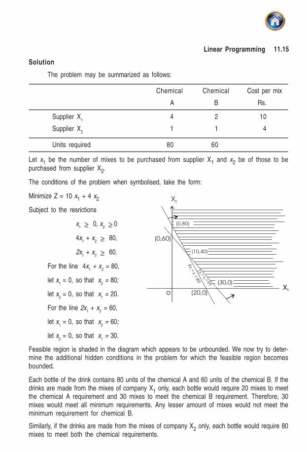
The problem may be summarized as follows:
Chemical Chemical Cost per mix
A B Rs.
Supplier X1
4 2 10
Supplier X2
1 1 4
Units required 80 60
Let x1 be the number of mixes to be purchased from supplier X1 and x2 be of those to bepurchased from supplier X2.
The conditions of the problem when symbolised, take the form:
Minimize Z = 10 x1 + 4 x2
Subject to the resrictions
x1 ≥ 0, x
2 ≥ 0
4x1 + x
2 ≥ 80,
2x1 + x
2 ≥ 60.
For the line 4x1 + x
2 = 80,
let x1 = 0, so that x
2 = 80;
let x2 = 0, so that x
1 = 20.
For the line 2x1 + x
2 = 60,
let x1 = 0, so that x
2 = 60;
let x2 = 0, so that x
1 = 30.
Feasible region is shaded in the diagram which appears to be unbounded. We now try to deter-mine the additional hidden conditions in the problem for which the feasible region becomesbounded.
Each bottle of the drink contains 80 units of the chemical A and 60 units of the chemical B. If thedrinks are made from the mixes of company X1 only, each bottle would require 20 mixes to meetthe chemical A requirement and 30 mixes to meet the chemical B requirement. Therefore, 30mixes would meet all minimum requirements. Any lesser amount of mixes would not meet theminimum requirement for chemical B.
Similarly, if the drinks are made from the mixes of company X2 only, each bottle would require 80mixes to meet both the chemical requirements.
��
��
��
2x + x = 60
1
2
4x+
x=
8 0
12
������
������
������
�������
������
11.16 Advanced Management Accounting
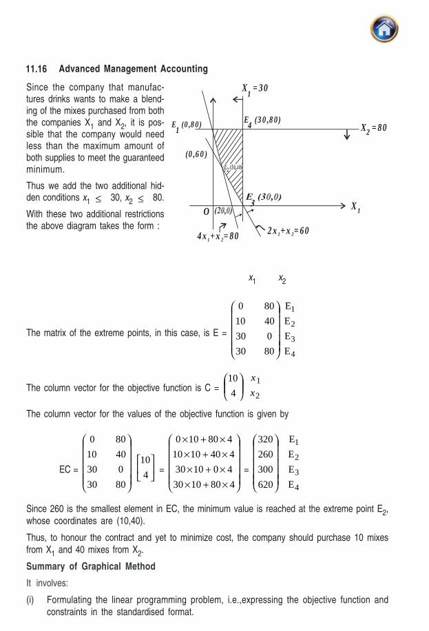
Since the company that manufac-tures drinks wants to make a blend-ing of the mixes purchased from boththe companies X1 and X2, it is pos-sible that the company would needless than the maximum amount ofboth supplies to meet the guaranteedminimum.
Thus we add the two additional hid-den conditions x1 ≤ 30, x2 ≤ 80.
With these two additional restrictionsthe above diagram takes the form :
x1 x2
The matrix of the extreme points, in this case, is E =
4
3
2
1
E
E
E
E
80
0
40
80
30
30
10
0
⎟⎟⎟⎟⎟
⎠
⎞
⎜⎜⎜⎜⎜
⎝
⎛
The column vector for the objective function is C = ⎟⎟⎠
⎞⎜⎜⎝
⎛4
10
2
1
x
x
The column vector for the values of the objective function is given by
EC = ⎟⎟⎟⎟⎟
⎠
⎞
⎜⎜⎜⎜⎜
⎝
⎛
80
0
40
80
30
30
10
0
⎥⎦
⎤⎢⎣
⎡4
10 =
⎟⎟⎟⎟⎟
⎠
⎞
⎜⎜⎜⎜⎜
⎝
⎛
×+××+××+××+×
4801030
401030
4401010
480100
=
4
3
2
1
E
E
E
E
620
300
260
320
⎟⎟⎟⎟⎟
⎠
⎞
⎜⎜⎜⎜⎜
⎝
⎛
Since 260 is the smallest element in EC, the minimum value is reached at the extreme point E2,whose coordinates are (10,40).
Thus, to honour the contract and yet to minimize cost, the company should purchase 10 mixesfrom X1 and 40 mixes from X2.
Summary of Graphical Method
It involves:
(i) Formulating the linear programming problem, i.e.,expressing the objective function andconstraints in the standardised format.
X 1
X = 301
E4
(3 0 ,8 0)E1
(0 ,8 0) X = 802
(0 ,6 0 )
2 x + x = 601 24 x + x = 801 2
O

11.17Linear Programming
(ii) Plotting the capacity constraints on the graph paper. For this purpose normally two terminalpoints are required. This is done by presuming simultaneously that one of the constraintsbis zero. When constraints concerns only one factor, then line will have only one originpoint and it will run parallel to the other axis.
(iii) Identifying feasible region and coordinates of corner points. Mostly it is done by breadingthe graph, but a point can be identified by solving simultaneous equation relating to twolines which intersect to form a point on graph.
(iv) Testing the corner point which gives maximum profit. For this purpose the coordinatesrelating to the corner point should put in objectives function and the optimal point shouldbe ascertained.
(v) For decision – making purpose, sometimes, it is required to know whether optimal pointleaves some resources unutilized. For this purpose value of coordinates at the optimalpoint should be put with constraint to find out which constraints are not fully utilized.
11.3 TRIAL & ERROR METHOD OF SOLVING LINEAR PROGRAMMING PROBLEM
11.3.1 Method of Solving LPP: Trial & Error Method (or Algebraic Approach)
Graphical method cannot be used when there are more than 2 variables in a LPP., in such a
case we use the simplex method which is highly efficient and versatile as also amenable to
further mathematical treatment and offers interesting economic interpretations. However, its
underlying concepts are rather lengthy to discuss and the student should patiently go through the
following material on the trial and error method to gain a good grasp over the simplex technique.
Slack Variable
Consider the following example :
Example : Maximize Z = 3x1 + 4x
2
subject to 2x1 + 3x
2 + ≤ 16
4x1 + 2x
2 ≤ 16
x1, x
2 ≥ 0.
The ≤ type inequalities can be transformed into equalities by the addition of non negative
variables, say x3 and x4 (known as slack variables) as below. The slack variables represent idle
resources, therefore, they are to be positive or non negative. Further the contribution per unit of a
slack variable is always taken as zero in the objective function of a LPP. This is so because profits
are not made on unused resources.
⎭⎬⎫
⎩⎨⎧
=++=++
16124
16132
421
321
xxx
xxx...(A)
And the objective function may be rewritten as below.
Maximize Z = 3x1 + 4x
2 + 0x
3+ 0x
4
11.18 Advanced Management Accounting
Surplus Variable
In ³ type inequalities, we subtract a variable (called the surplus variable) to make it an equality.
The value of this variable can be interpreted as the excess amount of the resources utilized over
and above the given level. The contribution per unit of a surplus variable is also taken as zero in
the objective function.
11.3.2 The linear programming Theorems : The trial and error and simplex methods are
based on the concept of slack variables and theorems described below:
Extreme point theorem : It states that an optimal solution to a LPP occurs at one of the vertices
of the feasible region. This should be obvious from the discussion on the graphical method.
Now the vertices are defined by the intersection of equations. The first step of the method is,
therefore, to convert the inequalities into equalities by the addition (or subtraction) of the slack (or
surplus variables) depending on the direction of the inequality.
It is to be noted that the system of equations (A) above has more variables than the number ofequations. Such a system of equations has an infinite number of solutions; yet it has finite andfew vertices, the co-ordinates of which can be determined by applying the Basis theorem.
Basis theorem : It states that for a system of m equations in n variables (where n > m) has asolution in which at least (n-m) of the variables have value of zero as a vertex. This solution iscalled a basic solution.
Extreme point theorem can be extended to state that the objective function is optimal at least atone of the basic solutions. Some of the vertices may be infeasible in that they have -ve co-ordinates and have to be dropped in view of the non-negativity condition on all variables includ-ing the slack and surplus variables.
Consider the following LPP for elucidating the basis theorem.
Maximize Z = 3x1 + 4x
2
Subject to 2x1 + 3x
2 < 16
4x1 + 2x
2 < 16
x1 , x
2 >
0.
Introducing slack variables x3 and x
4, we have
Maximize Z = 3x1 + 4x
2 +0x
3 + 0x
4
Subject to 2x1 + 3x
2 + 1x
3 + 0x
4 = 16
4x1 + 2x
2 + 0x
3 + 1x
4 = 16 ... (B)
x1 , x
2 , x
3 , x
4 > 0.
Here n (number of variables) = 4 and m (number of equations) = 2. Thus n - m = 2. Accordingto the Basis theorem we set 2 (= n – m) variables in (B) equal to zero at a time, solve the resultingsystem of equations and obtain a basic solution. Thus if we zeroise x1 and x2, the resultingsystem of equations would be

11.19Linear Programming
⎭⎬⎫
⎩⎨⎧
=+=+
1610
1601
43
43
xx
xx......(C) Set 1 (x1
= x2 = 0)
These equations directly yield x3 = 16 and x4 = 16 as the basic solution i.e. the co-ordinate of avertex.
The other sets of equations, upon zeroising two variables at a time in (B), would be as follows:
⎥⎦
⎤⎢⎣
⎡=+=+
1624
1632
21
21
xx
xxSet 2 (x
3 = x
4 = 0)
⎥⎦
⎤⎢⎣
⎡=+=+1614
1602
41
41
xx
xxSet 3 (x
2 = x
3 = 0)
⎥⎦
⎤⎢⎣
⎡=+=+
1604
1612
31
31
xx
xxSet 4 (x
2 = x
4 = 0)
⎥⎦
⎤⎢⎣
⎡=+=+
1602
1613
32
32
xx
xxSet 5 (x
1 = x
4 = 0)
⎥⎦
⎤⎢⎣
⎡=+=+1612
1603
42
42
xx
xxSet 6 (x
1 = x
3 = 0)
It is a simple matter to solve these six sets of simultaneous equations and obtain the six basicsolutions i.e. co-ordinates of the six vertices of the feasible region. The solutions are given below.The student may verify these by solving each of the sets of simultaneous equations.
Set Solution
1 x3 =16, x
4 = 16
2 x1 = 2, x
2 = 4
3 x1 = 8, x
4 = –16
4 x1 = 4, x
3 = 8
5 x2 = 8, x
3 = –8
6 x2 = 16/3, x
4 = 16/3
Since solutions of set 3 and 5 yield a negative co-ordinate each, contradicting thereby the non-
negativity of constraints, thus these are infeasible and are to be dropped from consideration.
Now according to the basis theorem the optimal solution lies at one of these vertices. By substi-
tuting these co-ordinates the values of objective function are derived below:
11.20 Advanced Management Accounting
Set Solution Z (Profit)
1 x3 = 16, x
4 = 16 0
2 x1 = 2, x
2 = 4 22
3 Infeasible
4 x1 = 4, x
3 = 8 12
5 Infeasible
6 x2 = 16/3, x
4 = 16/3 21
1
3
Thus solution of set 2 is optimal with a profit of 22. In this way we can solve a LPP simply by
employing the theorems stated above; but the simplex method is a further improvement over the
trial and error method. Following three are the inefficiencies in the trial and error method.
11.3.3 Inefficiencies of Trial and Error Method :
(a) In a LPP where m and n are larger, solving of numerous sets of simultaneous equations
would be extremely cumbersome and time-consuming.
(b) Scanning the profit table we notice that we jump from profit 0 to 22 to 211/3 i.e. there are ups
and downs. The simplex method ensures that successive solutions yield progressively higher
profits, culminating into the optimal one.
(c) Some of the sets yield infeasible solutions. There should be means to detect such sets and
not to solve them at all.
11.4 THE SIMPLEX METHOD
The simplex method is a computational procedure - an algorithm - for solving linear programming
problems. It is an iterative optimizing technique. In the simplex process, we must first find an initial
basis solution (extreme point). We then proceed to an adjacent extreme point. We continue
moving from point to point until we reach an optimal solution. For a maximization problem, the
simplex method always moves in the direction of steepest ascent, thus ensuring that the value of
the objective function improves with each solution.
The process is illustrated with the help of the following example:
Illustration
Maximize Z = 3x1 + 4x
2
Subject to 2x1 + 3x
2 ≤ 16 (machining time)
4x1 + 2x
2 ≤ 16 (assembly time)
x1 ≥ 0, x
2 ≥ 0
11.21Linear Programming
Solution
Step 1. Obtaining an initial solution: Obtain an initial solution that satisfies all the constraints of
the problem. The simplex process requires that all constraints be expressed as equations. There-
fore we must convert all inequalities into equalities.
Consider the constraint 2x1 + 3x2 < 16
Value on the left hand side of the inequality represents the amount of machine time a particular
solution uses, while the quantity on right side of inequality sign represents the total amount of
machine time available. Let x3 be a variable which represents the unused machine time in this
solution so that
2x1 + 3x
2 + x
3 = 16
Similarly, let x4 represent the amount of assembly time that is available but not used so that
4x1 + 2x2 + x4 = 16
The variables x3 and x4 are referred to as slack variables.
Thus slack variables represent the quantity of a resource not used by a particular solution, and
they are necessary to convert the constraint inequalities to equalities.
As we proceed with the simplex method, it will be helpful to place certain information in a table
known as a simplex tableau.
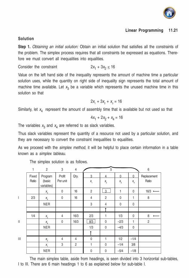
The simplex solution is as follows.
1 2 3 4 5 6
Fixed Program Profit Qty. 3 4 0 0 Replacement
Ratio (basic Per unit x1
x2
x3
x4
Ratio
variables)
x3
0 16 2 3 1 0 16/3
I 2/3 x4
0 16 4 2 0 1 8
NER 3 4 0 0
1/4 x2
4 16/3 2/3 1 1/3 0 8
II x4
0 16/3 8/3 0 –2/3 1 2
NER 1/3 0 –4/3 0
III x2
4 4 0 1 1/2 –1/4
x1
3 2 1 0 –1/4 3/8
NER 0 0 –5/4 –1/8
The main simplex table, aside from headings, is seen divided into 3 horizontal sub-tables,I to III. There are 6 main headings 1 to 6 as explained below for sub-table I.
11.22 Advanced Management Accounting
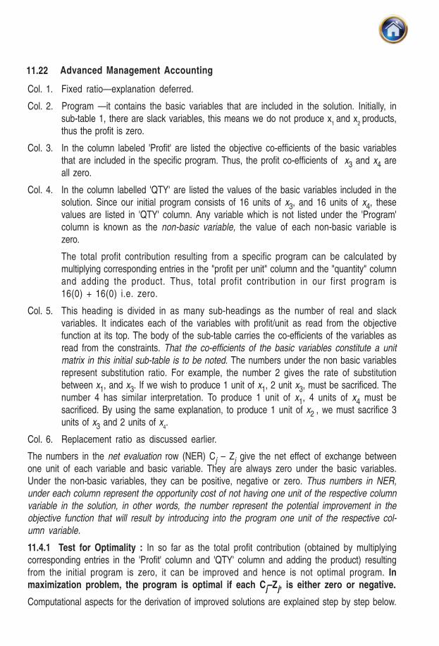
Col. 1. Fixed ratio—explanation deferred.
Col. 2. Program —it contains the basic variables that are included in the solution. Initially, insub-table 1, there are slack variables, this means we do not produce x
1 and x
2 products,
thus the profit is zero.
Col. 3. In the column labeled 'Profit' are listed the objective co-efficients of the basic variablesthat are included in the specific program. Thus, the profit co-efficients of x3 and x4 areall zero.
Col. 4. In the column labelled 'QTY' are listed the values of the basic variables included in thesolution. Since our initial program consists of 16 units of x3, and 16 units of x4, thesevalues are listed in 'QTY' column. Any variable which is not listed under the 'Program'column is known as the non-basic variable, the value of each non-basic variable iszero.
The total profit contribution resulting from a specific program can be calculated bymultiplying corresponding entries in the "profit per unit" column and the "quantity" columnand adding the product. Thus, total profit contribution in our first program is16(0) + 16(0) i.e. zero.
Col. 5. This heading is divided in as many sub-headings as the number of real and slackvariables. It indicates each of the variables with profit/unit as read from the objectivefunction at its top. The body of the sub-table carries the co-efficients of the variables asread from the constraints. That the co-efficients of the basic variables constitute a unit
matrix in this initial sub-table is to be noted. The numbers under the non basic variablesrepresent substitution ratio. For example, the number 2 gives the rate of substitutionbetween x1, and x3. If we wish to produce 1 unit of x1, 2 unit x3, must be sacrificed. Thenumber 4 has similar interpretation. To produce 1 unit of x1, 4 units of x4 must besacrificed. By using the same explanation, to produce 1 unit of x2
, we must sacrifice 3units of x3 and 2 units of x
4.
Col. 6. Replacement ratio as discussed earlier.
The numbers in the net evaluation row (NER) Cj – Zj give the net effect of exchange betweenone unit of each variable and basic variable. They are always zero under the basic variables.Under the non-basic variables, they can be positive, negative or zero. Thus numbers in NER,
under each column represent the opportunity cost of not having one unit of the respective column
variable in the solution, in other words, the number represent the potential improvement in the
objective function that will result by introducing into the program one unit of the respective col-
umn variable.
11.4.1 Test for Optimality : In so far as the total profit contribution (obtained by multiplyingcorresponding entries in the 'Profit' column and 'QTY' column and adding the product) resultingfrom the initial program is zero, it can be improved and hence is not optimal program. In
maximization problem, the program is optimal if each Cj–Zj, is either zero or negative.
Computational aspects for the derivation of improved solutions are explained step by step below.
11.23Linear Programming
Step 1. Select the incoming variable in sub-table I in the NER. The NER entries in the first sub-table are simply the profit unit figures as read from the objective function or copied from headings5. However there is a more rigorous method of making these entries which alone has to be
followed in making entries in the subsequent NER's and explanation on which is deferred. Selec-tion of the incoming variable is simple indeed. The positive (Cj–Zj) in NER indicate the mag-
nitude of opportunity cost of not including 1 unit of variables x1 and x2 respectively at
this stage. We select the one with highest entry in NER as incoming variable and thishappens to be x2, with a value of 4. We note this selection by putting an arrow below 4 in the NERof sub-table I. The column with the arrow is known as the key column.
Step 2. Select the outgoing variable, for this we have to calculate how many units of x2 can bebrought in without exceeding the existing capacity of any one of the resources? Thus, we mustcalculate the maximum allowable number of units of x2, that can be brought into the programwithout violating the non-negative constraints. For this, we compute the replacement ratio of col.6. This is done by dividing col. 4 by the key column and we get 16/3 and 8 and as the ratio. Thevariable x3, against the least ratio of 16/3 is selected as the outgoing variable and the fact is notedby putting an arrow against the least ratio of 16/3. This is maximum quantity of x2 that can beproduced at this stage without violating the non negative constraint. This row with the arrow iscalled the key row. The element at the intersection of the key row and the key column is knownas the pivot or key element and it is encircled.
Step 3. Having noted the incoming variable (x2 ) and the outgoing variable (x3 ) we are ready toperform the row operations on sub-table-I and fill in columns 4 and 5 of sub-table II.
Before that however, we fill in cols. 2 and 3 of sub-table II which is straight forward; x3 is replacedby x2 in col. 2, x4 stays in it and in col. 3 the profit/unit figure corresponding to x2 is copied fromheading while other figures remain the same.
11.4.2 Transformation of key row : The rule for transforming the key row is: Divide all the
numbers in the key row by the key number. The resulting numbers form the corresponding row in
the next table.
The key row of sub-table-I (under col. 4 and 5) is divided by the pivot element and this becomesthe corresponding row of the sub-table-II. It reads 16/3, 2/3, 1, 1/3, 0
11.4.3 Transformation of the non-key rows : The rule for transforming a non-key row is:
Subtract from the old row number (in each column) the product of the corresponding key-row
number and the corresponding fixed ratio formed by dividing the old row number in the keycolumn by the key number. The result will give the corresponding new row number.
This rule can be placed in the following equation form:
Fixed ration = numberkey
columnkeyinnumberrowOld
These are entered in the non key row under column I in the sub-table-I itself.
New row number = old row number
– (corresponding number in key row × corresponding fixed ratio)
11.24 Advanced Management Accounting
The key row in sub-table-I is multiplied by the fixed ratio of the non key row. This leads to
162
3
32
32
2
3
4
33
2
32 1
2
3
2
30
2
30× = × = × = × = × =, , , ,
This, however, is a rough work. Entries are not made any where. The result of this multiplicationare subtracted from the non-key row of sub-table-I to yield the non key row of the sub-table-II asbelow:
16 – 32
3 =
16
3, 4 –
4
3 =
8
3, 2 – 2 =0, 0 –
2
3= –
2
3, 1–0 = 1
These entries are made for the non-key row of sub-table-II.
Step IV. This consists of deriving the NER of sub-table-II. Each of its elements is derived bymultiplying col. 3 of sub-table-II with col. 5, summing these up and subtracting the sum from theprofit/unit is heading 5. Computations for each element in the 2nd NER are shown below:
3
1
3
80
3
243 =⎟
⎠⎞
⎜⎝⎛ ×+×−
4 – (4 × 1 + 0 × 0) = 0
3
4
3
20
3
140 −=⎟
⎠⎞
⎜⎝⎛ −
×+×−
0 – (4 × 0 + 0 × 1) = 0
But what is the underlying logic? The constraints in the sub-table – II have become
2
3x x x x1 2 3 4+ 1 +
1
3+ 0 =
16
3
8
3x
1 +0x
2 –
2
3 x
3 + 1x
4=
16
3
i.e. x2
=16
3–
2
3x
1–
1
3x
3(i)
x4 =
16
3–
8
3x
1+
2
3x
3(ii)
Substituting these values of x2 and x
4 in the original objective function
Z = 3x1 + 4x
2 + 0x
3 + 0x
4
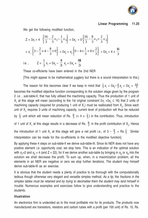
11.25Linear Programming
We get the following modified function,
Z = 3x1 + 4
⎭⎬⎫
⎩⎨⎧ −− 31 3
1
3
2
3
16xx
+ 0x
3 + 0
⎭⎬⎫
⎩⎨⎧ +− 31 3
2
3
8
3
16xx
= x1
⎭⎬⎫
⎩⎨⎧ ×−×− 0
3
84
3
23 + 0x
2 + x
3 ⎭⎬⎫
⎩⎨⎧ ×+×−
3
20
3
140 + 0x
4 + 4 ×
16
3
i.e. , Z = 1
3x
1 + 0x
2 –
4
3 x
3 + 0x
4 +
64
3
These co-efficients have been entered in the 2nd NER
[This might appear to be mathematical jugglery but there is a sound interpretation to this.]
The reason for this becomes clear if we keep in mind that 13 x
1 + 0x
2– 4
3 x3 + 0x
4 + 64
3
becomes the modified objective function corresponding to the solution stage given by the program
2 i.e. , sub-table-II, that has fully utilised the machining capacity. Thus the production of 1 unit of
X1 at this stage will mean (according to the 1st original constraint 2x
1 +3x
2 ≤ 16) that 2 units of
machining capacity (required for producing 1 unit of X1) must be reallocated from X
2. Since each
unit of X2 requires 3 units of machining capacity, current level of production will thus be reduced
by 23 unit which will mean reduction of Rs. 8
3 (= 4 × 23 ) in the contribution. Thus, introduction
of 1 unit of X1 at this stage results in a decrease of Rs. 8
3 in the profit contribution of X2. Hence
the introduction of 1 unit X1 at this stage will give a net profit i.e., of 3 – 8
3 = Rs. 13 Similar
interpretation can be made for the co-efficients in the modified objective function].
By applying these 4 steps on sub-table-II we derive sub-table-III. Since its NER does not have any
positive element i.e. opportunity cost, we stop here. This is an indication of the optimal solution
with x1=2 and x2 = 4 (and Z = 22), for if we derive another sub-table by bringing in x3 or x4 into the
solution we shall decrease the profit. To sum up, when, in a maximization problem, all the
elements in an NER are negative or zero we stop further iterations. The student may himself
derive sub-table-III as an exercise.
It is obvious that the student needs a plenty of practice to be thorough with the computationally
tedious though otherwise very elegant and versatile simplex method. As a tip, the fractions in the
simplex tables must be retained and by trying to decimalise them the student may land himself in
trouble. Numerous examples and exercises follow to give understanding and practice to the
students.
Illustration
An electronics firm is undecided as to the most profitable mix for its products. The products now
manufactured are transistors, resistors and carbon tubes with a profit (per 100 unit) of Rs. 10, Rs.
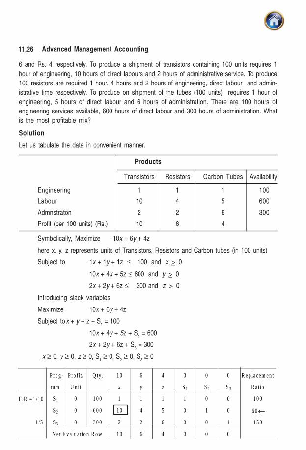
11.26 Advanced Management Accounting
6 and Rs. 4 respectively. To produce a shipment of transistors containing 100 units requires 1
hour of engineering, 10 hours of direct labours and 2 hours of administrative service. To produce
100 resistors are required 1 hour, 4 hours and 2 hours of engineering, direct labour and admin-
istrative time respectively. To produce on shipment of the tubes (100 units) requires 1 hour of
engineering, 5 hours of direct labour and 6 hours of administration. There are 100 hours of
engineering services available, 600 hours of direct labour and 300 hours of administration. What
is the most profitable mix?
Solution
Let us tabulate the data in convenient manner.
Products
Transistors Resistors Carbon Tubes Availability
Engineering 1 1 1 100
Labour 10 4 5 600
Admnstraton 2 2 6 300
Profit (per 100 units) (Rs.) 10 6 4
Symbolically, Maximize 10x + 6y + 4z
here x, y, z represents units of Transistors, Resistors and Carbon tubes (in 100 units)
Subject to 1x + 1y + 1z ≤ 100 and x ≥ 0
10x + 4x + 5z ≤ 600 and y ≥ 0
2x + 2y + 6z ≤ 300 and z ≥ 0
Introducing slack variables
Maximize 10x + 6y + 4z
Subject tox + y + z + S1 = 100
10x + 4y + 5z + S2 = 600
2x + 2y + 6z + S3 = 300
x ≥ 0, y ≥ 0, z ≥ 0, S1 ≥ 0, S
2 ≥ 0, S
3 ≥ 0
Pro g-
ram
Pro fit/
U n it
Q ty . 10
x
6
y
4
z
0
S1
0
S2
0
S3
Re p lacem e nt
Ra tio
S1 0 10 0 1 1 1 1 0 0 10 0F.R = 1 /1 0
S2 0 60 0 10 4 5 0 1 0 60←_
1 /5 S3 0 30 0 2 2 6 0 0 1 15 0
N et E v a lu a tio n R o w 10 6 4 0 0 0
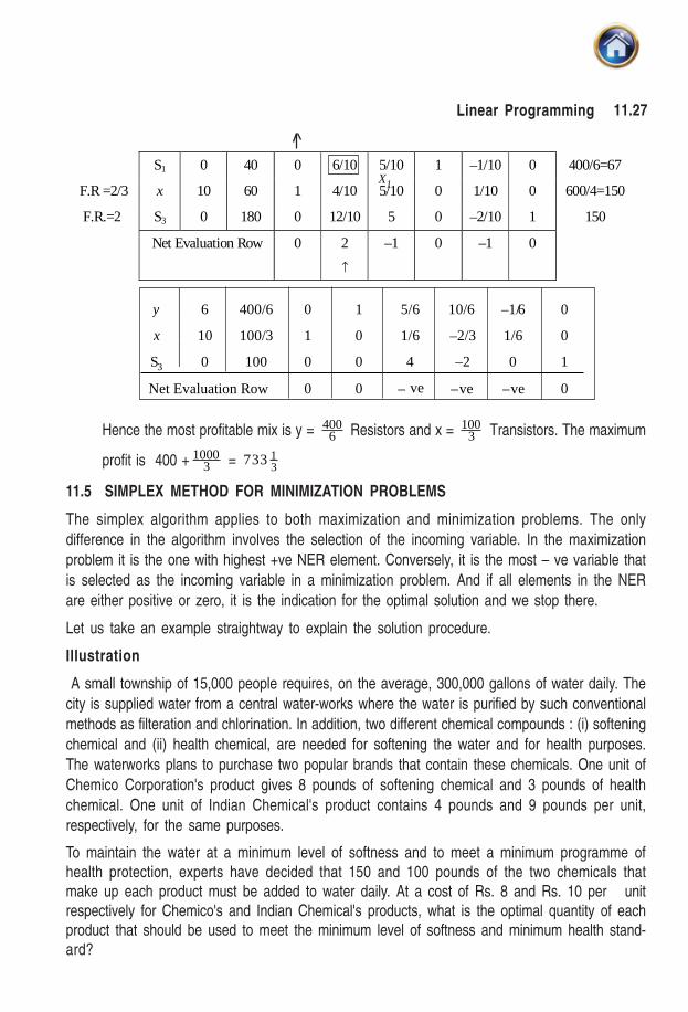
11.27Linear Programming
Hence the most profitable mix is y = 4006 Resistors and x = 100
3 Transistors. The maximum
profit is 400 + 10003 = 7331
3
11.5 SIMPLEX METHOD FOR MINIMIZATION PROBLEMS
The simplex algorithm applies to both maximization and minimization problems. The only
difference in the algorithm involves the selection of the incoming variable. In the maximization
problem it is the one with highest +ve NER element. Conversely, it is the most – ve variable that
is selected as the incoming variable in a minimization problem. And if all elements in the NER
are either positive or zero, it is the indication for the optimal solution and we stop there.
Let us take an example straightway to explain the solution procedure.
Illustration
A small township of 15,000 people requires, on the average, 300,000 gallons of water daily. The
city is supplied water from a central water-works where the water is purified by such conventional
methods as filteration and chlorination. In addition, two different chemical compounds : (i) softening
chemical and (ii) health chemical, are needed for softening the water and for health purposes.
The waterworks plans to purchase two popular brands that contain these chemicals. One unit of
Chemico Corporation's product gives 8 pounds of softening chemical and 3 pounds of health
chemical. One unit of Indian Chemical's product contains 4 pounds and 9 pounds per unit,
respectively, for the same purposes.
To maintain the water at a minimum level of softness and to meet a minimum programme ofhealth protection, experts have decided that 150 and 100 pounds of the two chemicals thatmake up each product must be added to water daily. At a cost of Rs. 8 and Rs. 10 per unitrespectively for Chemico's and Indian Chemical's products, what is the optimal quantity of eachproduct that should be used to meet the minimum level of softness and minimum health stand-ard?
S1 0 40 0 6/10 5/10 1 –1/10 0 400/6=67
F.R =2/3 x 10 60 1 4/10 5/10 0 1/10 0 600/4=150
F.R.=2 S3 0 180 0 12/10 5 0 –2/10 1 150
Net Evaluation Row 0 2
↑
–1 0 –1 0
X1
y 6 400/6 0 1 5/6 10/6 –1/6 0
x 10 100/3 1 0 1/6 –2/3 1/6 0
S3 0 100 0 0 4 –2 0 1
Net Evaluation Row 0 0 – ve –ve –ve 0
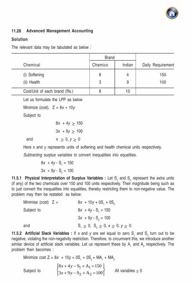
11.28 Advanced Management Accounting
Solution
The relevant data may be tabulated as below :
Brand
Chemical Chemico Indian Daily Requirement
(i) Softening 8 4 150
(ii) Health 3 9 100
Cost/Unit of each brand (Rs.) 8 10
Let us formulate the LPP as below
Minimize (cost), Z = 8x + 10y
Subject to
8x + 4y ≥ 150
3x + 9y ≥ 100
and x ≥ 0, y ≥ 0
Here x and y represents units of softening and health chemical units respectively.
Subtracting surplus variables to convert inequalities into equalities.
8x + 4y - S1 = 150
3x + 9y - S2 = 100
11.5.1 Physical Interpretation of Surplus Variables : Let S1 and S
2 represent the extra units
(if any) of the two chemicals over 150 and 100 units respectively. Their magnitude being such asto just convert the inequalities into equalities, thereby restricting them to non-negative value. Theproblem may then be restated as below:
Minimise (cost) Z = 8x + 10y + 0S1 + 0S
2
Subject to 8x + 4y - S1 = 150
3x + 9y - S2 = 100
and S1 ≥ 0, S
2 ≥ 0, x ≥ 0, y ≥ 0.
11.5.2 Artificial Slack Variables : If x and y are set equal to zero S1 and S
2 turn out to be
negative, violating the non-negativity restriction. Therefore, to circumvent this, we introduce anothersimilar device of artificial slack variables. Let us represent these by A
1 and A
2 respectively. The
problem then becomes :
Minimize cost Z = 8x + 10y + 0S1 + 0S
2 + MA
1 + MA
2
Subject to⎭⎬⎫
⎩⎨⎧
=+−+=+−+
100AS93
150AS48
22
11
yx
yxAll variables > 0
11.29Linear Programming
Physical Interpretation of the Artificial Variables.
These are imaginary brands, each unit containing 1 unit of the pertinent chemical. Both arerestricted to non-negatives. Whereas surplus variables have zeros as their cost co-efficient, eachartificial variable is assigned an infinitely large cost co-efficient (usually denoted by M).
Uses of artificial variables
1. It is our basic assumption that none of the basic variables in the L.P. problem can have anegative value. Thus, artificial variable is added to act as basic variable in a particularequation and hence it avoids the possibility of getting negative values for basic variables.
2. These artificial variables are such that their objective function co-efficients impose a hugeand hence unacceptable penalty. In the case of maximization problem, the objective functionis modified by subtracting a quantity (MA1) where M is arbitrarily large value and A1 is theartificial variable. For minimization problem, the objective function is modified by adding thequantity MA1. Thus artificial variables enable us to make a convenient and correct start inobtaining an initial solution.
3. The artificial variables with the high penalty once replaced by a real variable will never enterthe optimal program. Hence the solution to the modified problem will give the optimal solu-tion to the original problem.
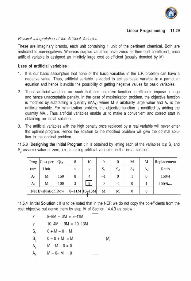
11.5.3 Designing the Initial Program : It is obtained by letting each of the variables x,y, S1 and
S2 assume value of zero, i.e., retaining artificial variables in the initial solution.
11.5.4 Initial Solution : It is to be noted that in the NER we do not copy the co-efficients from the
cost objective but derive them by step IV of Section 14.4.3 as below :
x 8–8M – 3M = 8–11M
y 10–4M – 9M = 10–13M
S1
0 + M – 0 = M
S2
0 – 0 + M = M (A)
A1
M – M – 0 = 0
A2
M – 0– M = 0
Prog
ram
Cost per
Unit
Qty. 8
x
10
y
0
S1
0
S2
M
A1
M
A2
Replacement
Ratio
A1 M 150 8 4 –1 0 1 0 150/4
A2 M 100 3 9 0 –1 0 1 100/9←
Net Evaluation Row 8–11M10–13M M M 0 0
11.30 Advanced Management Accounting
The reason for this is explained below. The problem is rewritten below:
Minimize Z = 8x + 10y + 0S1+ 0S
2 + MA
1 + MA
2
Subject to 8x + 4y – S1 + A
1= 150 ... (i)
3x + 9y – S2 + A
2= 100 ... (ii)
All variables ≥ 0.
From (i) A1 = 150 – 8x – 4y + S
1
From (ii) A2 = 100 – 3x – 9y + S
2
Substituting these in the objective function,
Z = 8x + 10y + 0S1 + 0S
2+ M (150–8x – 4y + S
1) + M(100 – 3x – 9y + S
2)
= (8 – 11M) x + (10 – 13M) y + MS1+ MS
2+ 0A
1+ 0A
2.
These co-efficients correspond to set A above.
Now consider the initial solution with an initial cost of (150 + 100) M for further inspiration.
10–13M is the most – ve and, therefore, the column, under 'y' is the key column. Also, the ratio100/9 is less than 150/4 (on extreme right). The pivot element, then, is 9. The outgoing variableis A2 being replaced by y. The cost of the existing solution, 250 M is forbiddingly high. The stageis set for revising the initial program.
The key row is revised by dividing it through by 9, the pivot element and the results are as follows:
100
3, 3
9, 1,0,
-1
9, 0,
1
9 .
The fixed ratio for revising the non-key row is 4/9. The revised figures for this row are computedbelow:
150 – 100 × 4
9 =
1350 400
9
950
9
–=
8 – 3 × 9
4 =
9
1272− =
9
6
4 – 9 × 4
9= 0
– 1 – 0 = –1
0 + 4
9=
4
91 – 0 = 1
0 – 1 × 4
9 =
9
4−
11.31Linear Programming
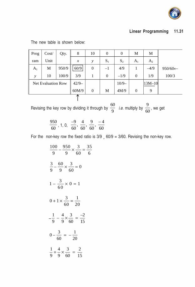
The new table is shown below:
Revising the key row by dividing it through by 60
9 i.e. multiply by
9
60, we get
950
60, 1, 0,
–9, , ,
–
60
4
60
9
60
4
60
For the non-key row the fixed ratio is 3/9 ¸ 60/9 = 3/60. Revising the non-key row.
100
9
950
9
3
60
35
6– × =
3
9
60
9
3
600– × =
13
600 1– × =
0 13
60
1
20+ × =
–1
9
4
9
3
60 15–
–2× =
03
60
1
20– –=
1
9
4
9
3
60
2
15+ × =
Prog
ram
Cost/
Unit
Qty. 8
x
10
y
0
S1
0
S2
M
A1
M
A2
A1 M 950/9 60/9 0 –1 4/9 1 –4/9 950/60←
y 10 100/9 3/9 1 0 –1/9 0 1/9 100/3
Net Evaluation Row 42/9–
60M/9 0 M
10/9–
4M/9 0
13M–10
9
11.32 Advanced Management Accounting
The result are tabulated below:
Hence the optimal cost is 95
68
35
610× + ×
= 760 350
3
+
= 1110
6 = 185 Answer.
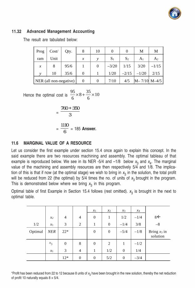
11.6 MARGINAL VALUE OF A RESOURCE
Let us consider the first example under section 15.4 once again to explain this concept. In thesaid example there are two resources machining and assembly. The optimal tableau of thatexample is reproduced below. We see in its NER -5/4 and –1/8 below x3 and x4. The marginalvalue of the machining and assembly resources are then respectively 5/4 and 1/8. The implica-tion of this is that if now (at the optimal stage) we wish to bring in x3 in the solution, the total profitwill be reduced from 22 (the optimal) by 5/4 times the no. of units of x3 brought in the program.This is demonstrated below where we bring x3 in this program.
Optimal table of first Example in Section 15.4 follows (rest omitted). x3 is brought in the next tooptimal table.
*Profit has been reduced from 22 to 12 because 8 units of x3 have been brought in the new solution, thereby the net reductionof profit 10 naturally equals 8 × 5/4.
Prog
ram
Cost/
Unit
Qty. 8
x
10
y
0
S1
0
S2
M
A1
M
A2
x 8 95/6 1 0 –3/20 1/15 3/20 –1/15
y 10 35/6 0 1 1/20 –2/15 –1/20 2/15
NER (all non-negative) 0 0 7/10 4/5 M– 7/10 M–4/5
1/2
x2
x1
4
3
4
2
x1
0
1
x2
1
0
x3
1/2
–1/4
x4
–1/4
3/8
8�
–8
Optimal NER 22* 0 0 –5/4 –1/8 Bring x3 insolution
X3
x1
0
3
8
4
0
1
2
1/2
1
0
–1/2
1/4
12* 0 0 5/2 0 –3/4
x3
11.33Linear Programming
Please note that marginal value of resource is synonymous with opportunity cost or shadow price.
11.7 SOME REMARKS
1. It may be desired to convert a maximization problem into a minimization one and viceversa. Mathematically, this can be accomplished by reversing signs though of just theobjective function.
2. Inequalities in the wrong direction: Consider the problem:
Maximize Z = x1 + 5x
2
Subject to 3x1 + 4x
2 ≤ 6 ... (i)
x1 + 3x
2 ≥ 2 ... (ii)
x1 , x
2 ≥ 0
[Whether to introduce slack or surplus or artificial variables depends on the type of
inequality and has nothing to do with type of the problem i.e., maximization or
minimization].
The 2nd inequality is in the wrong direction. Upon introducing the "surplus" variable.
x1 + 3x2 – S2 = 2
If S2 is taken in the initial solution it would be – ve when x1 and x2 are zero. To circumvent this,an artificial variable is also introduced in this inequality. The problem becomes:
Maximize Z = x1 + 5x2 - MA2
Subject to 3x1 + 4x2 + S1 = 6
x1 + 3x
2 – S
2 +A
2 = 2
x1 , x
2, S
1, S
2, A
2 > 0
(Note that in maximization problems M always has -ve sign and in minimization problems
M always has a + ve sign in the objective function).
The initial solution consists of S1 and A2. Several examples on inequalities in the wrong directionfollow. Surplus variables can never come in initial solution.
3. Any linear programming problem can be re-formulated into what is known as its dual. Any of
the primal (the original) or the dual may be selected for iterating by the simplex method. The
selection is made on the basis of computational burden. Also the dual provides interesting
insights into the methodology of the LP solution. This matter is discussed in a following
section at a greater length.
4. If two or more variables share the maximum positive co-efficient in the net evaluation row any
one may be chosen for introduction for the new solution arbitrarily, viz., in Z = 2x1 + 2x2 + x3it matters little if x1 or x2 is chosen.
5. Lower bounds may be specified in an LPP. For example, over and above to the three usual
constraints, it may be stipulated that x1 cannot be less than 25 or 40 or l1.i.e., x1 > l1. This can
11.34 Advanced Management Accounting
be handled quite easily by introducing a variable y1 such that x1 = l1 + y1. Substitute x1 = l1+ y1 wherever it occurs and solve the LPP. Computations would be greatly reduced. Please
see illustration on page no. 15.32 in this connection.
6. In all the simplex tables there is bound to be a unit matrix of size p × p where p is the no. of
rows (excluding net evaluation row). The columns that constitute such a unit matrix need not
be adjacent.
7. In view of the tediousness of computational aspects it is useful to make a check at each
iteration. This can be done by deriving the net evaluation row in two ways. (i) just like any
other row in the simplex tableau by deriving its fixed ratio (ii) by summing the product of the
quantities column with the profit/cost column and subtracting this sum from the original profit
contribution or cost co-efficient of variable. These should tally. Also, having obtained the
optimal solution it is desirable to verify it if it obeys the given constraints.
8. The simplex method, the graphical and trial and error methods, the dual approach provide
several ways of doing an LPP. The student may want to do each LPP in more than one way
for the sake of verification of the answer and practice.
Illustration
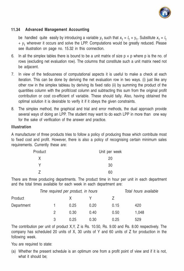
A manufacturer of three products tries to follow a policy of producing those which contribute mostto fixed cost and profit. However, there is also a policy of recognising certain minimum salesrequirements. Currently these are:
Product Unit per week
X 20
Y 30
Z 60
There are three producing departments. The product time in hour per unit in each departmentand the total times available for each week in each department are:
Time required per product, in hours Total hours available
Product X Y Z
Department 1 0.25 0.20 0.15 420
2 0.30 0.40 0.50 1,048
3 0.25 0.30 0.25 529
The contribution per unit of product X,Y, Z is Rs. 10.50, Rs. 9.00 and Rs. 8.00 respectively. Thecompany has scheduled 20 units of X, 30 units of Y and 60 units of Z for production in thefollowing week.
You are required to state:
(a) Whether the present schedule is an optimum one from a profit point of view and if it is not,what it should be;
11.35Linear Programming
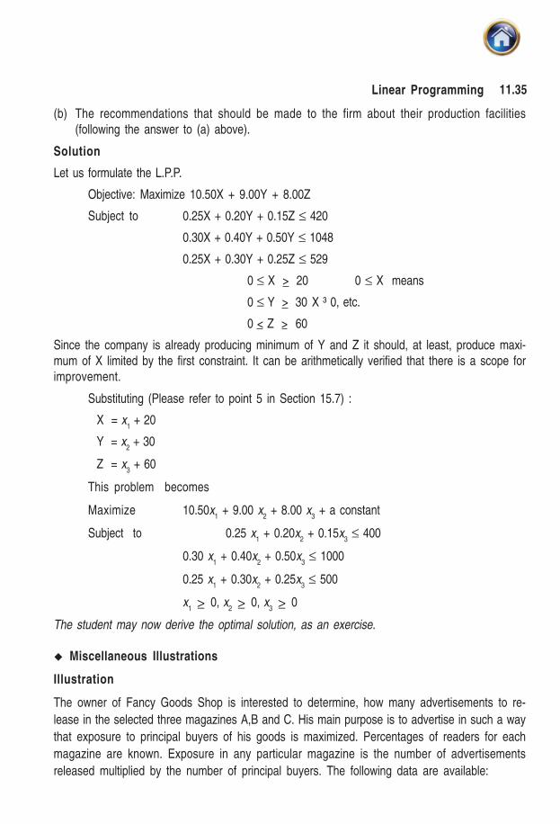
(b) The recommendations that should be made to the firm about their production facilities(following the answer to (a) above).
Solution
Let us formulate the L.P.P.
Objective: Maximize 10.50X + 9.00Y + 8.00Z
Subject to 0.25X + 0.20Y + 0.15Z ≤ 420
0.30X + 0.40Y + 0.50Y ≤ 1048
0.25X + 0.30Y + 0.25Z ≤ 529
0 ≤ X > 20 0 ≤ X means
0 ≤ Y > 30 X ³ 0, etc.
0 < Z > 60
Since the company is already producing minimum of Y and Z it should, at least, produce maxi-mum of X limited by the first constraint. It can be arithmetically verified that there is a scope forimprovement.
Substituting (Please refer to point 5 in Section 15.7) :
X = x1 + 20
Y = x2 + 30
Z = x3 + 60
This problem becomes
Maximize 10.50x1 + 9.00 x
2 + 8.00 x
3 + a constant
Subject to 0.25 x1 + 0.20x
2 + 0.15x
3 ≤ 400
0.30 x1 + 0.40x
2 + 0.50x
3 ≤ 1000
0.25 x1 + 0.30x
2 + 0.25x
3 ≤ 500
x1 ≥ 0, x
2 ≥ 0, x
3 ≥ 0
The student may now derive the optimal solution, as an exercise.
� Miscellaneous Illustrations
Illustration
The owner of Fancy Goods Shop is interested to determine, how many advertisements to re-
lease in the selected three magazines A,B and C. His main purpose is to advertise in such a way
that exposure to principal buyers of his goods is maximized. Percentages of readers for each
magazine are known. Exposure in any particular magazine is the number of advertisements
released multiplied by the number of principal buyers. The following data are available:
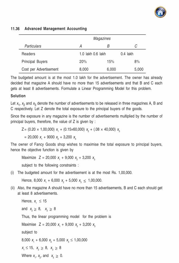
11.36 Advanced Management Accounting
Magazines
Particulars A B C
Readers 1.0 lakh 0.6 lakh 0.4 lakh
Principal Buyers 20% 15% 8%
Cost per Advertisement 8,000 6,000 5,000
The budgeted amount is at the most 1.0 lakh for the advertisement. The owner has already
decided that magazine A should have no more than 15 advertisements and that B and C each
gets at least 8 advertisements. Formulate a Linear Programming Model for this problem.
Solution
Let x1, x2 and x3 denote the number of advertisements to be released in three magazines A, B and
C respectively. Let Z denote the total exposure to the principal buyers of the goods.
Since the exposure in any magazine is the number of advertisements multiplied by the number of
principal buyers, therefore, the value of Z is given by :
Z = (0.20 × 1,00,000) x1 + (0.15×60,000) x
2 + (.08 × 40,000) x
3
= 20,000 x1 + 9000 x
2 + 3,200 x
3
The owner of Fancy Goods shop wishes to maximise the total exposure to principal buyers,
hence the objective function is given by
Maximize Z = 20,000 x1 + 9,000 x
2 + 3,200 x
3
subject to the following constraints :
(i) The budgeted amount for the advertisement is at the most Rs. 1,00,000.
Hence, 8,000 x1 + 6,000 x
2 + 5,000 x
3 ≤ 1,00,000.
(ii) Also, the magazine A should have no more than 15 advertisements, B and C each should get
at least 8 advertisements.
Hence, x1
≤ 15
and x2 ≥ 8, x
3 ≥ 8
Thus, the linear programming model for the problem is
Maximise Z = 20,000 x1 + 9,000 x
2 + 3,200 x
3
subject to
8,000 x1 + 6,000 x
2 + 5,000 x
3 ≤ 1,00,000
x1 ≤ 15, x
2 ≥ 8, x
3 ≥ 8
Where x1, x
2, and x
3 ≥ 0.

11.37Linear Programming
Illustration
A Mutual Fund Company has Rs. 20 lakhs available for investment in Government Bonds, blue
chip stocks, speculative stocks and short-term deposits. The annual expected return and risk
factor are given below:
Type of investment Annual Expected Return (%) Risk Factor (0 to 100)
Government Bonds 14 12
Blue Chip Stocks 19 24
Speculative Stocks 23 48
Short-term Deposits 12 6
Mutual fund is required to keep at least Rs. 2 lakhs in short-term deposits and not to exceed
average risk factor of 42. Speculative stocks must be at most 20 percent of the total amount
invested. How should mutual fund invest the funds so as to maximize its total expected annual
return? Formulate this as a Linear Programming Problem. Do not solve it.
Solution
Let x1, x2, x3 and x4 denote the amount of funds to be invested in government bonds, blue chip
stocks, speculative stocks and short term deposits respectively. Let Z denote the total expected
return.
Since the Mutual Fund Company has Rs. 20 lakhs available for investment,
x1+ x
2+ x
3+ x
4 ≤ 20,00,000 ... (i)
Also, Mutual fund is required to keep at least Rs. 2 lakhs in short-term deposits,
Hence, x4 ≥ 2,00,000 ...(ii)
The average risk factor is given by
12x1 + 24x
2 + 48x
3 + 6x
4
x1 + x
2 + x
3 + x
4
Since the average risk factor Mutual Fund should not exceed 42, we get the following constraint.
12x1 + 24x
2 + 48x
3 + 6x
4
x1 + x
2 + x
3 + x
4
≤ 42
or 12x1 + 24x
2 + 48x
3 + 6x
4 ≤ 42 (x
1+x
2+x
3+x
4)
or –30x1 – 18x
2 + 6x
3 – 36x
4 ≤ 0 ...(iii)

11.38 Advanced Management Accounting
Further, speculative stock must be at most 20 per cent of the total amount invested, hence
x3 ≤ 0.20 (x
1 + x
2 + x
3 + x
4)
or – 0.2x1 – 0.2 x
2 – 0.8x
3– 0.2x
4 ≤ 0 ...(iv)
Finally, the objective is to maximise the total expected annual return, the objective function for
Mutual Fund can be expressed as
Maximise Z = 0.14x1 + 0.19x
2 + 0.23x
3 + 0.12x
4...(v)
Summarising equations (i) to (v), the linear programming model for the Mutual Fund company is
formulated as below:
Objective function :
Maximize Z = 0.14x1 + 0.19x
2 + 0.23x
3 + 0.12x
4
Subject to the constraints
x1
+ x2
+ x3
+ x4 ≤ 20,00,000
x4 ≥ 2,00,000
– 30x1 – 18x
2 + 6x
3 – 36x
4 ≤ 0
– 0.2x1 – 0.2x
2+ 0.8x
3 – 0.2x
4 ≤ 0
where x1 ≥ 0, x
2 ≥ 0, x
3 ≥ 0 and x
4 ≥ 0
Illustration
A firm produces three products A, B and C. It uses two types of raw materials I and II of which
5,000 and 7,500 units respectively are available. The raw material requirements per unit of the
products are given below:
Raw Material Requirements per unit of Product
A B C
I 3 4 5
II 5 3 5
The labour time for each unit of product A is twice that of product B and three times that of
product C. The entire labour force of the firm can produce the equivalent of 3,000 units. The
(marks) minimum demand of the three products is 600, 650 and 500 units respectively. Also, the
ratios of the number of units produced must be equal to 2 : 3 : 4. Assuming the profits per unit of
A,B and C as Rs. 50, 50 and 80 respectively.
Formulate the problem as a linear programming model in order to determine the number of units
of each product which will maximize the profit.
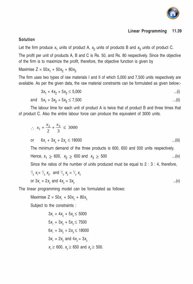
11.39Linear Programming
Solution
Let the firm produce x1 units of product A, x2 units of products B and x3 units of product C.
The profit per unit of products A, B and C is Rs. 50, and Rs. 80 respectively. Since the objective
of the firm is to maximize the profit, therefore, the objective function is given by
Maximise Z = 50x1 + 50x2 + 80x3
The firm uses two types of raw materials I and II of which 5,000 and 7,500 units respectively are
available. As per the given data, the raw material constraints can be formulated as given below:-
3x1 + 4x2 + 5x3 ≤ 5,000 ...(i)
and 5x1 + 3x2 + 5x3 ≤ 7,500 ...(ii)
The labour time for each unit of product A is twice that of product B and three times that
of product C. Also the entire labour force can produce the equivalent of 3000 units.
∴ xx x
12 3
2 33000+ + ≤
or 6x1 + 3x
2 + 2x
3 ≤ 18000 ...(iii)
The minimum demand of the three products is 600, 650 and 500 units respectively.
Hence, x1 ≥ 600, x2 ≥ 650 and x3 ≥ 500 ...(iv)
Since the ratios of the number of units produced must be equal to 2 : 3 : 4, therefore,
1/2 x
1= 1/
3 x
2, and 1/
3 x
2 = 1/
4 x
3
or 3x1 = 2x
2 and 4x
2 = 3x
3...(v)
The linear programming model can be formulated as follows:
Maximise Z = 50x1 + 50x
2 + 80x
3
Subject to the constraints :
3x1 + 4x
2 + 5x
3 ≤ 5000
5x1 + 3x
2 + 5x
3 ≤ 7500
6x1 + 3x
2 + 2x
3 ≤ 18000
3x1 = 2x
2 and 4x
2 = 3x
3
x1 ≥ 600, x
2 ≥ 650 and x
3 ≥ 500.
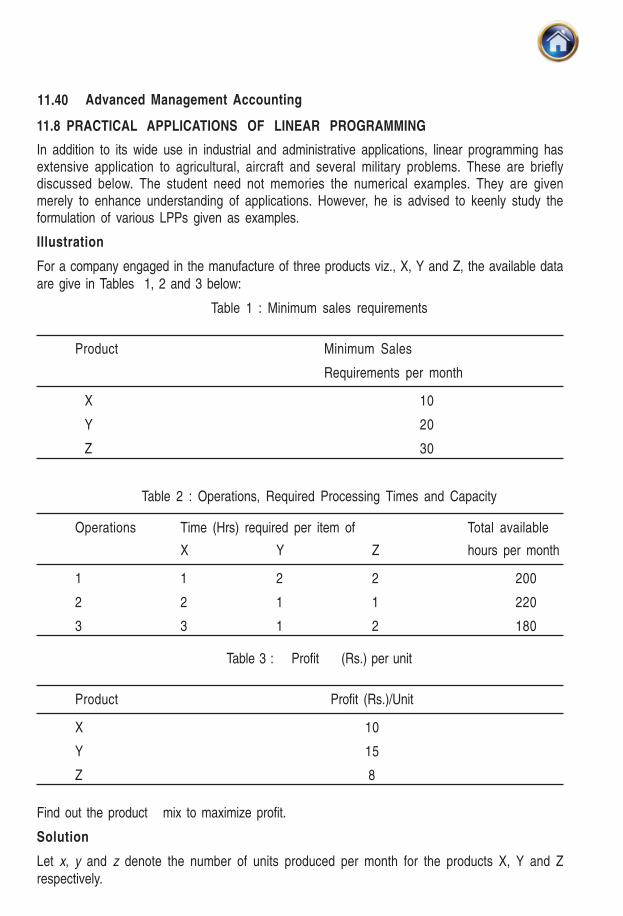
11.40 Advanced Management Accounting
11.8 PRACTICAL APPLICATIONS OF LINEAR PROGRAMMING
In addition to its wide use in industrial and administrative applications, linear programming hasextensive application to agricultural, aircraft and several military problems. These are brieflydiscussed below. The student need not memories the numerical examples. They are givenmerely to enhance understanding of applications. However, he is advised to keenly study theformulation of various LPPs given as examples.
Illustration
For a company engaged in the manufacture of three products viz., X, Y and Z, the available dataare give in Tables 1, 2 and 3 below:
Table 1 : Minimum sales requirements
Product Minimum Sales
Requirements per month
X 10
Y 20
Z 30
Table 2 : Operations, Required Processing Times and Capacity
Operations Time (Hrs) required per item of Total available
X Y Z hours per month
1 1 2 2 200
2 2 1 1 220
3 3 1 2 180
Table 3 : Profit (Rs.) per unit
Product Profit (Rs.)/Unit
X 10
Y 15
Z 8
Find out the product mix to maximize profit.
Solution
Let x, y and z denote the number of units produced per month for the products X, Y and Zrespectively.
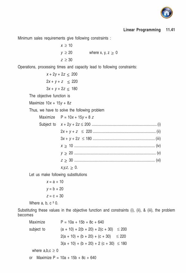
11.41Linear Programming
Minimum sales requirements give following constraints :
x ≥ 10
y ≥ 20 where x, y, z ≥ 0
z ≥ 30
Operations, processing times and capacity lead to following constraints:
x + 2y + 2z ≤ 200
2x + y + z ≤ 220
3x + y + 2z ≤ 180
The objective function is
Maximize 10x + 15y + 8z
Thus, we have to solve the following problem
Maximize P = 10x + 15y + 8 z
Subject to x + 2y + 2z ≤ 200 ................................................................... (i)
2x + y + z ≤ 220 ................................................................. (ii)
3x + y + 2z ≤ 180 ................................................................ (iii)
x ≥ 10 ................................................................................... (iv)
y ≥ 20 .................................................................................... (v)
z ≥ 30 ................................................................................... (vi)
x,y,z, ≥ 0.
Let us make following substitutions
x = a + 10
y = b + 20
z = c + 30
Where a, b, c ³ 0.
Substituting these values in the objective function and constraints (i), (ii), & (iii), the problembecomes
Maximize P = 10a + 15b + 8c + 640
subject to (a + 10) + 2(b + 20) + 2(c + 30) ≤ 200
2(a + 10) + (b + 20) + (c + 30) ≤ 220
3(a + 10) + (b + 20) + 2 (c + 30) ≤ 180
where a,b,c ≥ 0
or Maximize P = 10a + 15b + 8c + 640
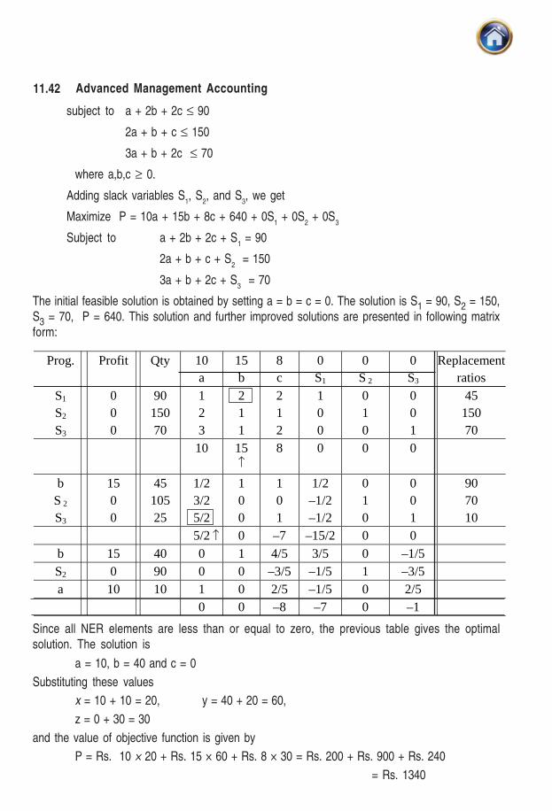
11.42 Advanced Management Accounting
subject to a + 2b + 2c ≤ 90
2a + b + c ≤ 150
3a + b + 2c ≤ 70
where a,b,c ≥ 0.
Adding slack variables S1, S
2, and S
3, we get
Maximize P = 10a + 15b + 8c + 640 + 0S1 + 0S
2 + 0S
3
Subject to a + 2b + 2c + S1 = 90
2a + b + c + S2 = 150
3a + b + 2c + S3 = 70
The initial feasible solution is obtained by setting a = b = c = 0. The solution is S1 = 90, S2 = 150,S3 = 70, P = 640. This solution and further improved solutions are presented in following matrixform:
Since all NER elements are less than or equal to zero, the previous table gives the optimalsolution. The solution is
a = 10, b = 40 and c = 0
Substituting these values
x = 10 + 10 = 20, y = 40 + 20 = 60,
z = 0 + 30 = 30
and the value of objective function is given by
P = Rs. 10 × 20 + Rs. 15 × 60 + Rs. 8 × 30 = Rs. 200 + Rs. 900 + Rs. 240
= Rs. 1340
Prog. Profit Qty 10a
15b
8c
0S1
0S 2
0S3
Replacementratios
S1
S2
S3
000
9015070
123
211
212
100
010
001
4515070
10 15 8 0 0 0
bS 2
S3
1500
4510525
1/23/25/2
100
101
1/2–1/2–1/2
010
001
907010
5/2 0 –7 –15/2 0 0b 15 40 0 1 4/5 3/5 0 –1/5S2 0 90 0 0 –3/5 –1/5 1 –3/5a 10 10 1 0 2/5 –1/5 0 2/5
0 0 –8 –7 0 –1
↑
↑
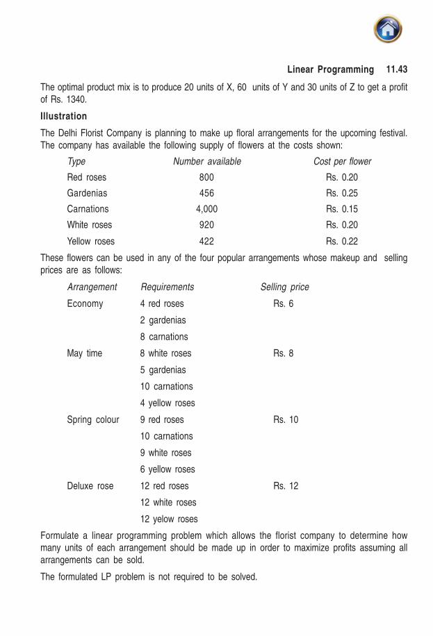
11.43Linear Programming
The optimal product mix is to produce 20 units of X, 60 units of Y and 30 units of Z to get a profitof Rs. 1340.
Illustration
The Delhi Florist Company is planning to make up floral arrangements for the upcoming festival.The company has available the following supply of flowers at the costs shown:
Type Number available Cost per flower
Red roses 800 Rs. 0.20
Gardenias 456 Rs. 0.25
Carnations 4,000 Rs. 0.15
White roses 920 Rs. 0.20
Yellow roses 422 Rs. 0.22
These flowers can be used in any of the four popular arrangements whose makeup and sellingprices are as follows:
Arrangement Requirements Selling price
Economy 4 red roses Rs. 6
2 gardenias
8 carnations
May time 8 white roses Rs. 8
5 gardenias
10 carnations
4 yellow roses
Spring colour 9 red roses Rs. 10
10 carnations
9 white roses
6 yellow roses
Deluxe rose 12 red roses Rs. 12
12 white roses
12 yelow roses
Formulate a linear programming problem which allows the florist company to determine howmany units of each arrangement should be made up in order to maximize profits assuming allarrangements can be sold.
The formulated LP problem is not required to be solved.
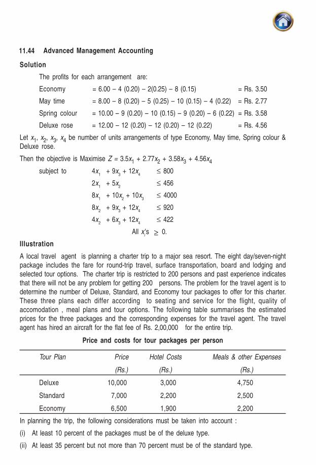
11.44 Advanced Management Accounting
Solution
The profits for each arrangement are:
Economy = 6.00 – 4 (0.20) – 2(0.25) – 8 (0.15) = Rs. 3.50
May time = 8.00 – 8 (0.20) – 5 (0.25) – 10 (0.15) – 4 (0.22) = Rs. 2.77
Spring colour = 10.00 – 9 (0.20) – 10 (0.15) – 9 (0.20) – 6 (0.22) = Rs. 3.58
Deluxe rose = 12.00 – 12 (0.20) – 12 (0.20) – 12 (0.22) = Rs. 4.56
Let x1, x2, x3, x4 be number of units arrangements of type Economy, May time, Spring colour &Deluxe rose.
Then the objective is Maximise Z = 3.5x1 + 2.77x2 + 3.58x3 + 4.56x4
subject to 4x1
+ 9x3 + 12x
4≤ 800
2x1
+ 5x2
≤ 456
8x1
+ 10x2 + 10x
3≤ 4000
8x2
+ 9x3 + 12x
4≤ 920
4x2
+ 6x3 + 12x
4≤ 422
All xi's
≥ 0.
Illustration
A local travel agent is planning a charter trip to a major sea resort. The eight day/seven-nightpackage includes the fare for round-trip travel, surface transportation, board and lodging andselected tour options. The charter trip is restricted to 200 persons and past experience indicatesthat there will not be any problem for getting 200 persons. The problem for the travel agent is todetermine the number of Deluxe, Standard, and Economy tour packages to offer for this charter.These three plans each differ according to seating and service for the flight, quality ofaccomodation , meal plans and tour options. The following table summarises the estimatedprices for the three packages and the corresponding expenses for the travel agent. The travelagent has hired an aircraft for the flat fee of Rs. 2,00,000 for the entire trip.
Price and costs for tour packages per person
Tour Plan Price Hotel Costs Meals & other Expenses
(Rs.) (Rs.) (Rs.)
Deluxe 10,000 3,000 4,750
Standard 7,000 2,200 2,500
Economy 6,500 1,900 2,200
In planning the trip, the following considerations must be taken into account :
(i) At least 10 percent of the packages must be of the deluxe type.
(ii) At least 35 percent but not more than 70 percent must be of the standard type.
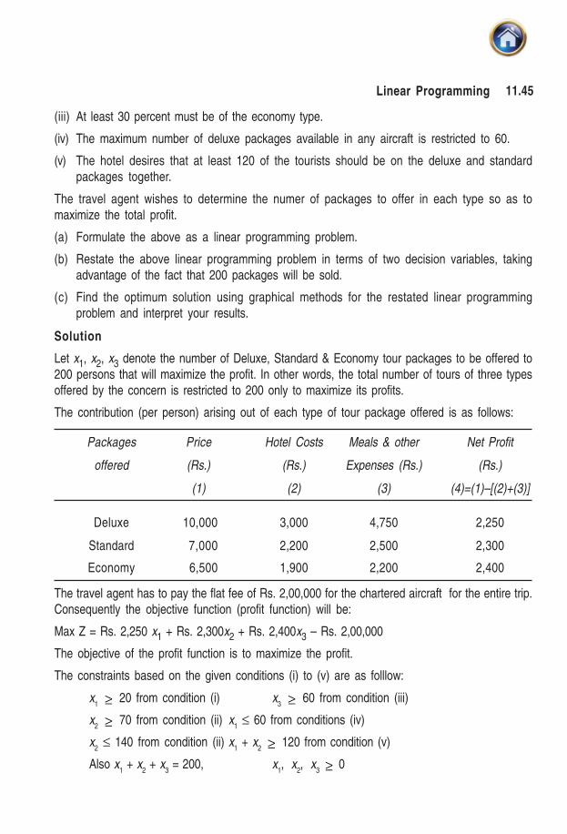
11.45Linear Programming
(iii) At least 30 percent must be of the economy type.
(iv) The maximum number of deluxe packages available in any aircraft is restricted to 60.
(v) The hotel desires that at least 120 of the tourists should be on the deluxe and standardpackages together.
The travel agent wishes to determine the numer of packages to offer in each type so as tomaximize the total profit.
(a) Formulate the above as a linear programming problem.
(b) Restate the above linear programming problem in terms of two decision variables, takingadvantage of the fact that 200 packages will be sold.
(c) Find the optimum solution using graphical methods for the restated linear programmingproblem and interpret your results.
Solution
Let x1, x2, x3 denote the number of Deluxe, Standard & Economy tour packages to be offered to200 persons that will maximize the profit. In other words, the total number of tours of three typesoffered by the concern is restricted to 200 only to maximize its profits.
The contribution (per person) arising out of each type of tour package offered is as follows:
Packages Price Hotel Costs Meals & other Net Profit
offered (Rs.) (Rs.) Expenses (Rs.) (Rs.)
(1) (2) (3) (4)=(1)–[(2)+(3)]
Deluxe 10,000 3,000 4,750 2,250
Standard 7,000 2,200 2,500 2,300
Economy 6,500 1,900 2,200 2,400
The travel agent has to pay the flat fee of Rs. 2,00,000 for the chartered aircraft for the entire trip.Consequently the objective function (profit function) will be:
Max Z = Rs. 2,250 x1 + Rs. 2,300x2 + Rs. 2,400x3 – Rs. 2,00,000
The objective of the profit function is to maximize the profit.
The constraints based on the given conditions (i) to (v) are as folllow:
x1 ≥ 20 from condition (i) x
3 ≥ 60 from condition (iii)
x2 ≥ 70 from condition (ii) x
1 ≤ 60 from conditions (iv)
x2 ≤ 140 from condition (ii) x
1 + x
2 ≥ 120 from condition (v)
Also x1 + x
2 + x
3 = 200, x
1, x
2, x
3 ≥ 0
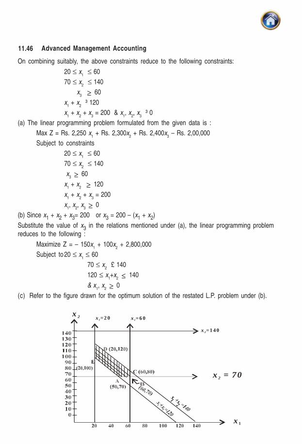
11.46 Advanced Management Accounting
On combining suitably, the above constraints reduce to the following constraints:
20 ≤ x1 ≤ 60
70 ≤ x2 ≤ 140
x3 ≥ 60
x1 + x
2 ³ 120
x1 + x
2 + x
3 = 200 & x
1, x
2, x
3 ³ 0
(a) The linear programming problem formulated from the given data is :
Max Z = Rs. 2,250 x1 + Rs. 2,300x
2 + Rs. 2,400x
3 – Rs. 2,00,000
Subject to constraints
20 ≤ x1 ≤ 60
70 ≤ x2 ≤ 140
x3 ≥ 60
x1 + x
2 ≥ 120
x1 + x
2 + x
3 = 200
x1, x
2, x
3 ≥ 0
(b) Since x1 + x2 + x3= 200 or x3 = 200 – (x1 + x2)
Substitute the value of x3 in the relations mentioned under (a), the linear programming problemreduces to the following :
Maximize Z = – 150x1 + 100x
2 + 2,800,000
Subject to20 ≤ x1 ≤ 60
70 ≤ x2 £ 140
120 ≤ x1+x
2 ≤ 140
& x1, x
2 ≥ 0
(c) Refer to the figure drawn for the optimum solution of the restated L.P. problem under (b).
x 1
x = 702
x 1= 2 0 x 1= 6 0
x 2= 1 4 0
x 2
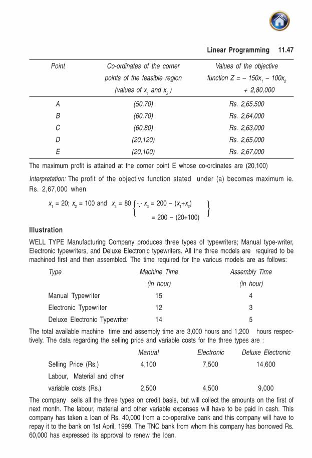
11.47Linear Programming
Point Co-ordinates of the corner Values of the objective
points of the feasible region function Z = – 150x1 – 100x
2
(values of x1 and x
2 ) + 2,80,000
A (50,70) Rs. 2,65,500
B (60,70) Rs. 2,64,000
C (60,80) Rs. 2,63,000
D (20,120) Rs. 2,65,000
E (20,100) Rs. 2,67,000
The maximum profit is attained at the corner point E whose co-ordinates are (20,100)
Interpretation: The profit of the objective function stated under (a) becomes maximum ie.
Rs. 2,67,000 when
x1 = 20; x
2 = 100 and x
3 = 80 x
3 = 200 – (x
1+x
2)
= 200 – (20+100)
Illustration
WELL TYPE Manufacturing Company produces three types of typewriters; Manual type-writer,Electronic typewriters, and Deluxe Electronic typewriters. All the three models are required to bemachined first and then assembled. The time required for the various models are as follows:
Type Machine Time Assembly Time
(in hour) (in hour)
Manual Typewriter 15 4
Electronic Typewriter 12 3
Deluxe Electronic Typewriter 14 5
The total available machine time and assembly time are 3,000 hours and 1,200 hours respec-tively. The data regarding the selling price and variable costs for the three types are :
Manual Electronic Deluxe Electronic
Selling Price (Rs.) 4,100 7,500 14,600
Labour, Material and other
variable costs (Rs.) 2,500 4,500 9,000
The company sells all the three types on credit basis, but will collect the amounts on the first ofnext month. The labour, material and other variable expenses will have to be paid in cash. Thiscompany has taken a loan of Rs. 40,000 from a co-operative bank and this company will have torepay it to the bank on 1st April, 1999. The TNC bank from whom this company has borrowed Rs.60,000 has expressed its approval to renew the loan.
≥
{ }∴

11.48 Advanced Management Accounting
The Balance Sheet of this Company as on 31.3.99 is as follows:
Liabilities Rs. Assets Rs.
Equity Share capital 1,50,000 Land 90,000
Capital Reserve 15,000 Building 70,000
General Reserve 1,10,000 Plant & Machinery 1,00,000
Profit & Loss a/c 25,000 Furniture & Fixtures 15,000
Long term loan 1,00,000 Vehicles 30,000
Loan from TNC Bank 60,000 Inventory 5,000
Loan from Co-op. Bank 40,000 Receivables 50,000
Cash 1,40,000
Tota l 5,00,000 To t a l 5,00,000
The company will have to pay a sum of Rs. 10,000 towards the salary from top management
executives and other fixed overheads for the month. Interest on long term loans is to be paid every
month at 24% per annum. Interest on loans from TNC and Co-operative Banks may be taken to
be Rs. 1,200 for the month. Also this company has promised to deliver 2 Manual typewriters and
8 Deluxe Electronic typewriters to one of its valued costomers next month.
Also make sure that the level of operations in this company is subject to the availability of cash
next month. This company will also be able to sell all their types of typewriter in the market. The
Senior Manager of this company desires to know as to how many units of each typewriter must be
manufactured in the factory next month so as to maximize the profits of the company. Formulate
this as a linear programming problem. The formulated problem need not be solved.
Solution
Let X1, X2 and X3 denote the number of Manual, Electronic and Deluxe Electronic typewriters
respectively to be manufactured in the factory next month. We are given the following data.
Manual Electronic Deluxe Electronic
Typewriter Typewriter Typewriter
Selling Price p.u. (Rs.) 4,100 7,500 14,600
Labour, Material and other 2,500 4,500 9,000
variable costs p.u. (Rs.)
Profit contribution p.u. (Rs.) 1,600 3,000 5,600
The objective of the company is to maximize the profit hence the objective function is given by
Maximize Z = 1600 X1 + 3000 X2 + 5600 X3 – (Rs. 10,000 + Rs. 2,000 + Rs. 1,200)
From the data given for time required for various models and the total number of hours availablefor machine time and assembly time, we get the following constraints:
15X1 + 12 X2 + 14X3 ≤ 3,000 (machine time restriction)
and 4X1 + 3X2 + 5X3 ≤ 1,200 (assembly time restriction)
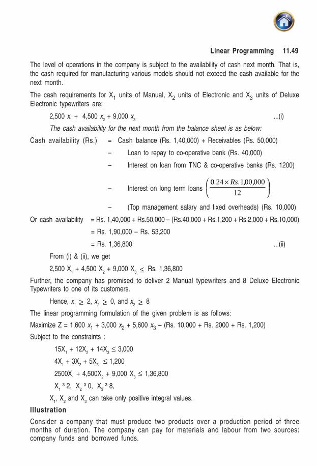
11.49Linear Programming
The level of operations in the company is subject to the availability of cash next month. That is,the cash required for manufacturing various models should not exceed the cash available for thenext month.
The cash requirements for X1 units of Manual, X2 units of Electronic and X3 units of DeluxeElectronic typewriters are;
2,500 x1 + 4,500 x
2 + 9,000 x
3...(i)
The cash availability for the next month from the balance sheet is as below:
Cash availability (Rs.) = Cash balance (Rs. 1,40,000) + Receivables (Rs. 50,000)
– Loan to repay to co-operative bank (Rs. 40,000)
– Interest on loan from TNC & co-operative banks (Rs. 1200)
– Interest on long term loans ⎟⎠⎞
⎜⎝⎛ ×
12
000001240 ,,.Rs.
– (Top management salary and fixed overheads) (Rs. 10,000)
Or cash availability = Rs. 1,40,000 + Rs.50,000 – (Rs.40,000 + Rs.1,200 + Rs.2,000 + Rs.10,000)
= Rs. 1,90,000 – Rs. 53,200
= Rs. 1,36,800 ...(ii)
From (i) & (ii), we get
2,500 X1 + 4,500 X
2 + 9,000 X
3 ≤ Rs. 1,36,800
Further, the company has promised to deliver 2 Manual typewriters and 8 Deluxe ElectronicTypewriters to one of its customers.
Hence, x1 ≥ 2, x
2 ≥ 0, and x
2 ≥ 8
The linear programming formulation of the given problem is as follows:
Maximize Z = 1,600 x1 + 3,000 x2 + 5,600 x3 – (Rs. 10,000 + Rs. 2000 + Rs. 1,200)
Subject to the constraints :
15X1 + 12X
2 + 14X
3 ≤ 3,000
4X1 + 3X
2 + 5X
3 ≤ 1,200
2500X1 + 4,500X
2 + 9,000 X
3 ≤ 1,36,800
X1 ³ 2, X
2 ³ 0, X
3 ³ 8,
X1, X
2 and X
3 can take only positive integral values.
Illustration
Consider a company that must produce two products over a production period of threemonths of duration. The company can pay for materials and labour from two sources:company funds and borrowed funds.
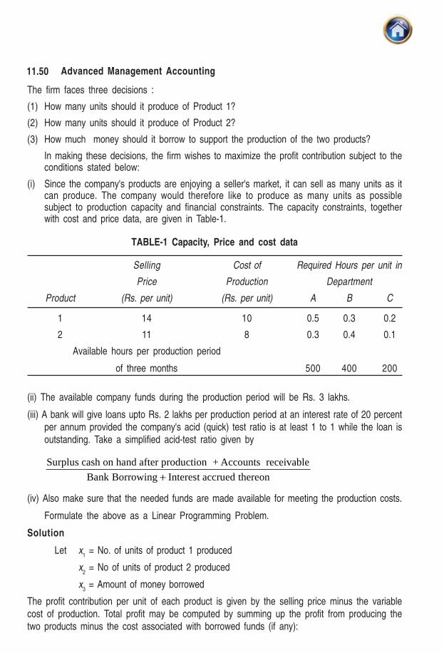
11.50 Advanced Management Accounting
The firm faces three decisions :
(1) How many units should it produce of Product 1?
(2) How many units should it produce of Product 2?
(3) How much money should it borrow to support the production of the two products?
In making these decisions, the firm wishes to maximize the profit contribution subject to theconditions stated below:
(i) Since the company's products are enjoying a seller's market, it can sell as many units as itcan produce. The company would therefore like to produce as many units as possiblesubject to production capacity and financial constraints. The capacity constraints, togetherwith cost and price data, are given in Table-1.
TABLE-1 Capacity, Price and cost data
Selling Cost of Required Hours per unit in
Price Production Department
Product (Rs. per unit) (Rs. per unit) A B C
1 14 10 0.5 0.3 0.2
2 11 8 0.3 0.4 0.1
Available hours per production period
of three months 500 400 200
(ii) The available company funds during the production period will be Rs. 3 lakhs.
(iii) A bank will give loans upto Rs. 2 lakhs per production period at an interest rate of 20 percentper annum provided the company's acid (quick) test ratio is at least 1 to 1 while the loan isoutstanding. Take a simplified acid-test ratio given by
Surplus cash on hand after production + Accounts receivable
BankBorrowing Interestaccruedthereon+
(iv) Also make sure that the needed funds are made available for meeting the production costs.
Formulate the above as a Linear Programming Problem.
Solution
Let x1 = No. of units of product 1 produced
x2 = No of units of product 2 produced
x3 = Amount of money borrowed
The profit contribution per unit of each product is given by the selling price minus the variablecost of production. Total profit may be computed by summing up the profit from producing thetwo products minus the cost associated with borrowed funds (if any):
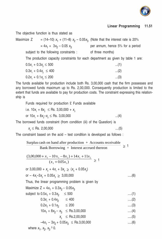
11.51Linear Programming
The objective function is thus stated as
Maximize Z = (14–10) x1 + (11–8) x2 – 0.05x3 (Note that the interest rate is 20%
= 4x1 + 3x2 – 0.05 x3 per annum, hence 5% for a period
subject to the following constraints : of three months)
The production capacity constraints for each department as given by table 1 are:
0.5x1 + 0.3x
2 ≤ 500 ...(1)
0.3x1 + 0.4x
2 ≤ 400 ...(2)
0.2x1 + 0.1x
2 ≤ 200 ...(3)
The funds available for production include both Rs. 3,00,000 cash that the firm possesses andany borrowed funds maximum up to Rs. 2,00,000. Consequently production is limited to theextent that funds are available to pay for production costs. The constraint expressing this relation-ship is
Funds required for production £ Funds available
i.e. 10x1 + 8x
2 ≤ Rs. 3,00,000 + x
3
or 10x1 + 8x
2–x
3 ≤ Rs. 3,00,000 ...(4)
The borrowed funds constraint (from condition (iii) of the Question) is
x3 ≤ Rs. 2,00,000 ....(5)
The constraint based on the acid – test condition is developed as follows :
Surpluscash on hand after production + Accounts receivableBank Borrowing + Interest accrued thereon ≥ 1
(3,00,000 –10x – 8 ) 14 11
( . )3 1 2 1+ + +
+x x x x
x x2
3 3005 ≥ 1
or 3,00,000 + x3 + 4x
1 + 3x
2 ≥ (x
3 + 0.05x
3)
or – 4x1–3x
2 + 0.05x
3 ≥ 3,00,000 .....(6)
Thus, the linear programming problem is given by
Maximize Z = 4x1 + 0.3x2 – 0.05x3
subject to 0.5x1 + 0.3x2 ≤ 500 .....(1)
0.3x1 + 0.4x2 ≤ 400 .....(2)
0.2x1 + 0.1x2 ≤ 200 .....(3)
10x1 + 8x2 – x3 ≤ Rs.3,00,000 .....(4)
x3
≤ Rs.2,00,000 .....(5)
–4x1 – 3x2 + 0.05x3
≤ Rs.3,00,000 .....(6)
where x1, x2, x3 ³ 0.

11.52 Advanced Management Accounting
Industrial Applications
These are basically product-mix problems in which the general objective is to derive the optimalproduction and procurement plan for the time period under consideration. The measure ofeffectiveness is either a defined return that is sought to be maximized or a defined cost that isto be minimized. Some examples follow:
Production Planning - product - mix problem :
An industrial concern has available a certain production capacity on various manufacturingprocesses and has the opportunity to utilize this capacity to manufacture various products. Typically,different products will have different selling prices, will require different amounts of productioncapacity at the several processes, and therefore will have different unit profits; there may also bestipulations on maximum and/or minimum production levels. The problem is to determine theoptimal mix so that the total profit is maximized.
Illustration
The Voltex Company produces an air conditioner/heating unit. The company currently has firmorders for 6 months into the future. The company can schedule its production over the next 6months to meet orders on either a regular or on overtime basis. Consider orders and the associ-ated production costs for the next 6 months as follows:
Month Jan. Feb. Mar. Apr. May Jun.
Orders 590 610 650 700 500 700
Cost/unit (Rs.)
Regular Production 50 52 51 55 47 50
Cost/Unit (Rs.)
Overtime Production 62 58 63 60 55 52
Maximum no. of units which can be produced on regular and overtime basis are 500 and 300respectively.
With 75 airconditioners in stock at the beginning of January, the company wishes to have at least100 air conditioners in stock at the end of June. The inventory-carrying costs for air-conditionersis Rs. 10 per unit per month.
Solution
Let xij = number of units produced in month i (i = 1, 2 ......, 6),
on a regular or overtime basis (j = 1, 2)
yi – number of units of ending inventory in month i (i = 1,2...., 6)
Minimize (cost) Z = 50x11
+ 62x12
+ 52x21
+ 58x22
+
51x31
+ 63x32
+ 55x41
+ 60x42
+
47x51
+ 55x52
+ 50x61
+ 52x62
+
10(y1 + y
2 + y
3 + y
4 + y
5 + y
6)
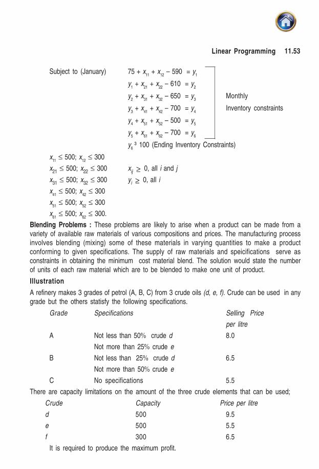
11.53Linear Programming
Subject to (January) 75 + x11
+ x12
– 590 = y1
y1 + x
21 + x
22 – 610 = y
2
y2 + x
31 + x
32 – 650 = y
3Monthly
y3 + x
41 + x
42 – 700 = y
4Inventory constraints
y4 + x
51 + x
52 – 500 = y
5
y5 + x
61 + x
62 – 700 = y
6
y6
³ 100 (Ending Inventory Constraints)
x11
≤ 500; x12
≤ 300
x21 ≤ 500; x22 ≤ 300 xij ≥ 0, all i and j
x31 ≤ 500; x32 ≤ 300 yi ≥ 0, all i
x41
≤ 500; x42
≤ 300
x51
≤ 500; x52
≤ 300
x61
≤ 500; x62
≤ 300.
Blending Problems : These problems are likely to arise when a product can be made from avariety of available raw materials of various compositions and prices. The manufacturing processinvolves blending (mixing) some of these materials in varying quantities to make a productconforming to given specifications. The supply of raw materials and speicifications serve asconstraints in obtaining the minimum cost material blend. The solution would state the numberof units of each raw material which are to be blended to make one unit of product.
Illustration
A refinery makes 3 grades of petrol (A, B, C) from 3 crude oils (d, e, f). Crude can be used in anygrade but the others statisfy the following specifications.
Grade Specifications Selling Price
per litre
A Not less than 50% crude d 8.0
Not more than 25% crude e
B Not less than 25% crude d 6.5
Not more than 50% crude e
C No specifications 5.5
There are capacity limitations on the amount of the three crude elements that can be used;
Crude Capacity Price per litre
d 500 9.5
e 500 5.5
f 300 6.5
It is required to produce the maximum profit.
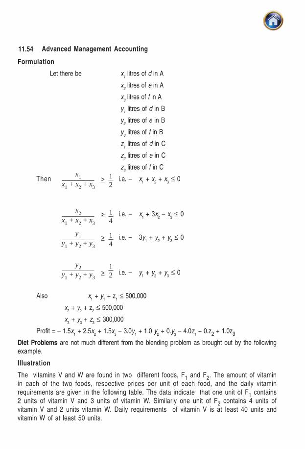
11.54 Advanced Management Accounting
Formulation
Let there be x1 litres of d in A
x2 litres of e in A
x3 litres of f in A
y1 litres of d in B
y2 litres of e in B
y3 litres of f in B
z1 litres of d in C
z2 litres of e in C
z3 litres of f in C
Then > i.e. – x1 + x
2 + x
3 ≤ 0
> i.e. – x1 + 3x
2 – x
3 ≤ 0
> i.e. – 3y1 + y
2 + y
3 ≤ 0
> i.e. – y1 + y
2 + y
3 ≤ 0
Also x1 + y
1 + z
1 ≤ 500,000
x2 + y
2 + z
2 ≤ 500,000
x3 + y
3 + z
3 ≤ 300,000
Profit = – 1.5x1 + 2.5x
2 + 1.5x
3 – 3.0y
1 + 1.0 y
2 + 0.y
3 – 4.0z
1 + 0.z2 + 1.0z3
Diet Problems are not much different from the blending problem as brought out by the followingexample.
Illustration
The vitamins V and W are found in two different foods, F1 and F2. The amount of vitaminin each of the two foods, respective prices per unit of each food, and the daily vitaminrequirements are given in the following table. The data indicate that one unit of F1 contains2 units of vitamin V and 3 units of vitamin W. Similarly one unit of F2 contains 4 units ofvitamin V and 2 units vitamin W. Daily requirements of vitamin V is at least 40 units andvitamin W of at least 50 units.
x1
x1 + x2 + x3
12
x2
x1 + x2 + x3
14
y1
y1 + y2 + y3
14
y2
y1 + y2 + y3
12

11.55Linear Programming
The problem is to determine optimal quantities of foods F1 and F2 to be bought so that thedaily vitamin requirements are met and, simultaneously the cost of buying the goods isminimized.
Food Daily
Vitamin F1
F2
Requirements
V 2 4 40
W 3 2 50
Cost/Unit of food 3 2.5
Formulation :
Let x1 and x
2 be quantities of F
1 and F
2 respectively.
Minimize 3x1 + 2.5x
2
subject to 2x1 + 4x
2 ≥ 40
3x1 + 2x
2 ≥ 50
x1 ≥ 0
x2 ≥ 0
Trim Problems are applicable to paper industry where paper of standard width has to becut into smaller width as per customer requirements with the objective of minimizing thewaste produced.
Illustration
The Fine Paper Company produces rolls of paper used in cash registers. Each roll ofpaper is 500 ft. in length and can be produced in widths of 1, 2, 3 and 5 inch. Thecompany's production process results in 500' rolls that are 12 inches in width. Thus thecompany must cut its 12 inch roll to the desired width. It has six basic cutting alternativesas follows:
Cutting No. of Rolls Waste
Alternative 1" 2" 3" 5" (Inches)
1 6 3 0 0 0
2 0 3 2 0 0
3 1 1 1 1 1
4 0 0 2 1 1
5 0 4 1 0 1
6 4 2 1 0 1
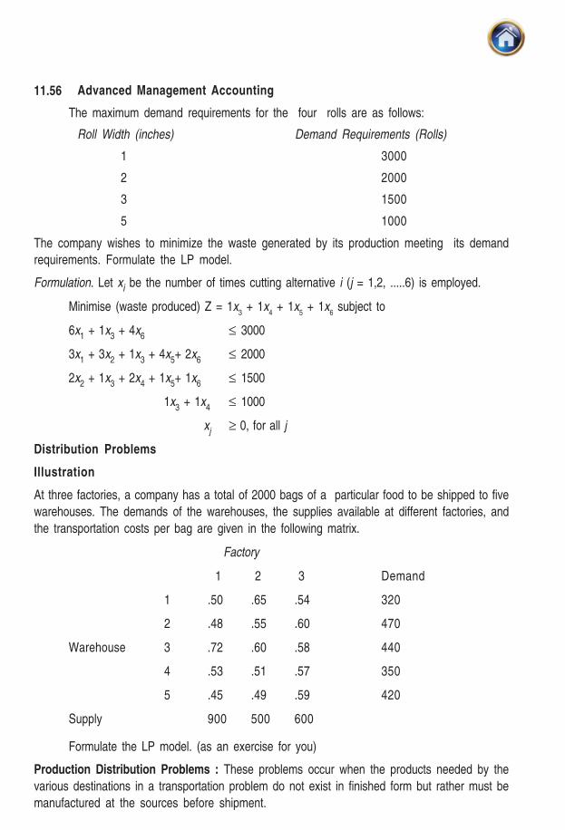
11.56 Advanced Management Accounting
The maximum demand requirements for the four rolls are as follows:
Roll Width (inches) Demand Requirements (Rolls)
1 3000
2 2000
3 1500
5 1000
The company wishes to minimize the waste generated by its production meeting its demand
requirements. Formulate the LP model.
Formulation. Let xi be the number of times cutting alternative i (j = 1,2, .....6) is employed.
Minimise (waste produced) Z = 1x3 + 1x
4 + 1x
5 + 1x
6 subject to
6x1 + 1x3 + 4x6 ≤ 3000
3x1 + 3x
2 + 1x
3 + 4x
5+ 2x
6≤ 2000
2x2 + 1x3 + 2x4 + 1x5+ 1x6 ≤ 1500
1x3 + 1x
4≤ 1000
xj ≥ 0, for all j
Distribution Problems
Illustration
At three factories, a company has a total of 2000 bags of a particular food to be shipped to five
warehouses. The demands of the warehouses, the supplies available at different factories, and
the transportation costs per bag are given in the following matrix.
Factory
1 2 3 Demand
1 .50 .65 .54 320
2 .48 .55 .60 470
Warehouse 3 .72 .60 .58 440
4 .53 .51 .57 350
5 .45 .49 .59 420
Supply 900 500 600
Formulate the LP model. (as an exercise for you)
Production Distribution Problems : These problems occur when the products needed by the
various destinations in a transportation problem do not exist in finished form but rather must be
manufactured at the sources before shipment.
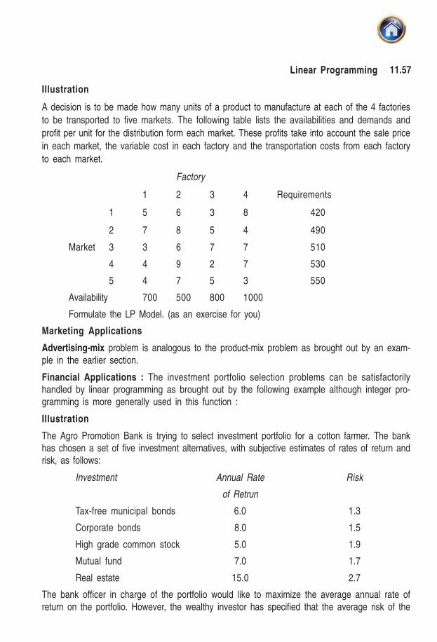
11.57Linear Programming
Illustration
A decision is to be made how many units of a product to manufacture at each of the 4 factories
to be transported to five markets. The following table lists the availabilities and demands and
profit per unit for the distribution form each market. These profits take into account the sale price
in each market, the variable cost in each factory and the transportation costs from each factory
to each market.
Factory
1 2 3 4 Requirements
1 5 6 3 8 420
2 7 8 5 4 490
Market 3 3 6 7 7 510
4 4 9 2 7 530
5 4 7 5 3 550
Availability 700 500 800 1000
Formulate the LP Model. (as an exercise for you)
Marketing Applications
Advertising-mix problem is analogous to the product-mix problem as brought out by an exam-ple in the earlier section.
Financial Applications : The investment portfolio selection problems can be satisfactorilyhandled by linear programming as brought out by the following example although integer pro-gramming is more generally used in this function :
Illustration
The Agro Promotion Bank is trying to select investment portfolio for a cotton farmer. The bankhas chosen a set of five investment alternatives, with subjective estimates of rates of return andrisk, as follows:
Investment Annual Rate Risk
of Retrun
Tax-free municipal bonds 6.0 1.3
Corporate bonds 8.0 1.5
High grade common stock 5.0 1.9
Mutual fund 7.0 1.7
Real estate 15.0 2.7
The bank officer in charge of the portfolio would like to maximize the average annual rate ofreturn on the portfolio. However, the wealthy investor has specified that the average risk of the

11.58 Advanced Management Accounting
portfolio should not exceed 2.0; and does not want more than 20% of the investment to be put intoreal estate. Formulate an LP model for the problem.
Formulation
Let xij be the percent of portfolio allocated to investment j ( j = 1,2,3,4,5).
Maximize (average annual rate of return on the portfolio) Z = 6%x1 + 8%x2 + 5% x3 + 7%x4 +
15% x5
subject to (Average risk constraint) 1.3x1 + 1.5x2 + 1.9x3 + 1.7x4 + 2.7x5 ≤ 2.0
(Real estate constraint) x5 ≤ 0.2
(Total investment constraint) x1 + x
2 + x
3 + x
4 + x
5 = 1.0
x1, x
2, x
3, x
4, x
5 ≥ 0.
Administrative Applications
The use of linear programming as a tool of administrative problem-solving is well-documented inboth academic circles and the area of business operations. Included in these areas of applicationare the following:
Personnel Assignment Problems
Bidding Problems as illustrated by following example:
Illustration
A company is to subcontract work on four assemblies. The five sub–contractors have agreed tosubmit a bid price on each assembly type and a limit on the total number of assemblies (in anycombination) for which they are willing to contract. These bids, the contract times, and therequirements for assemblies are given in the following matrix.
Sub–contractor
A B C D E Assemblies
Required
1 3.45 3.80 3.00 3.10 3.70 500
2 3.40 3.13 3.50 3.10 3.20 300
Assembly 3 3.35 3.50 3.50 3.20 3.40 300
4 3.60 3.00 3.00 3.30 3.90 400
Contract
Limits 250 280 330 360 380
Formulate the LP model. (Hint : Treat the problem as a transportation problem).
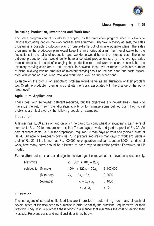
11.59Linear Programming
Balancing Production, Inventories and Work-force
The sales program cannot usually be accepted as the production program since it is likely toimpose fluctuating load on the work facilities and equipment. Anyhow, in theory at least, the salesprogram is a possible production plan on one extreme out of infinite possible plans. The salesprograms in the production plan would keep the inventories at a minimum level (zero) but thefluctuations in the rates of production and workforce would be at their highest cost. The otherextreme production plan would be to have a constant production rate (at the average salesrequirements) so the cost of changing the production rate and work-force are minimal, but theinventory-carrying costs are at their highest. In between, these two extremes are infinite numberof plans involving varying amounts of inventory-carrying costs on the one hand and costs associ-ated with changing production rate and work-force level on the other hand.
Example on the production smoothing problem would serve as an illustration of their problemtoo. Overtime production premiums constitute the "costs associated with the change of the work-force level".
Agriculture Applications
These deal with somewhat different resource, but the objectives are nevertheless same - tomaximize the return from the allocation activity or to minimize some defined cost. Two typicalproblems are illustrated by the following couple of examples.
Illustration
A farmer has 1,000 acres of land on which he can grow corn, wheat or soyabeans. Each acre ofcorn costs Rs. 100 for preparation, requires 7 man-days of work and yields a profit of Rs. 30. Anacre of wheat costs Rs. 120 for preparation, requires 10 man-days of work and yields a profit ofRs. 40. An acre of soyabeans costs Rs. 70 to prepare, requires 8 man days of work and yields aprofit of Rs. 20. If the farmer has Rs. 100,000 for preparation and can count on 8000 man-days ofwork, how many acres should be allocated to each crop to maximize profits? Formulate an LPmodel.
Formulation: Let x1, x2 and x3 designate the average of corn, wheat and soyabeans respectively.
Maximize Z = 30x1 + 40x
2 + 20x
3
subject to (Money) 100x1 + 120x
2 + 70x
3£ 100,000
(Man-day) 7x1 + 10x
2 + 8x
3£ 8000
(Acreage) x1 + x
2 + x
3£ 1000
x1, x
2, x
3 ≥ 0
Illustration
The managers of several cattle feed lots are interested in determining how many of each ofseveral types of livestock feed to purchase in order to satisfy the nutritional requirements for theirlivestock. They wish to purchase these foods in a manner that minimizes the cost of feeding theirlivestock. Relevant costs and nutritional data is as below.
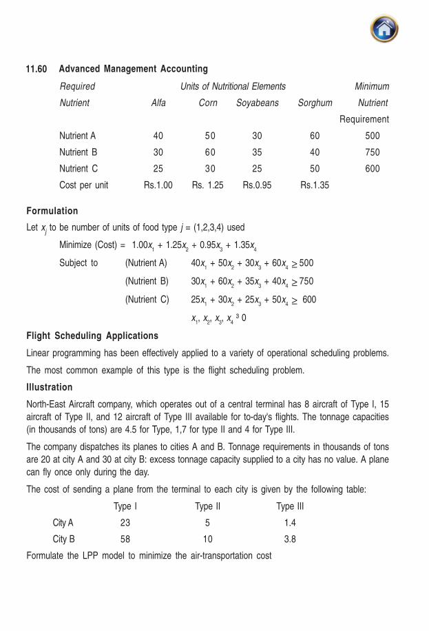
11.60 Advanced Management Accounting
Required Units of Nutritional Elements Minimum
Nutrient Alfa Corn Soyabeans Sorghum Nutrient
Requirement
Nutrient A 40 50 30 60 500
Nutrient B 30 60 35 40 750
Nutrient C 25 30 25 50 600
Cost per unit Rs.1.00 Rs. 1.25 Rs.0.95 Rs.1.35
Formulation
Let xj to be number of units of food type j = (1,2,3,4) used
Minimize (Cost) = 1.00x1 + 1.25x
2 + 0.95x
3 + 1.35x
4
Subject to (Nutrient A) 40x1 + 50x
2 + 30x
3 + 60x
4 ≥ 500
(Nutrient B) 30x1 + 60x
2 + 35x
3 + 40x
4 ≥ 750
(Nutrient C) 25x1 + 30x
2 + 25x
3 + 50x
4 ≥ 600
x1, x
2, x
3, x
4 ³ 0
Flight Scheduling Applications
Linear programming has been effectively applied to a variety of operational scheduling problems.
The most common example of this type is the flight scheduling problem.
Illustration
North-East Aircraft company, which operates out of a central terminal has 8 aircraft of Type I, 15
aircraft of Type II, and 12 aircraft of Type III available for to-day's flights. The tonnage capacities
(in thousands of tons) are 4.5 for Type, 1,7 for type II and 4 for Type III.
The company dispatches its planes to cities A and B. Tonnage requirements in thousands of tons
are 20 at city A and 30 at city B: excess tonnage capacity supplied to a city has no value. A plane
can fly once only during the day.
The cost of sending a plane from the terminal to each city is given by the following table:
Type I Type II Type III
City A 23 5 1.4
City B 58 10 3.8
Formulate the LPP model to minimize the air-transportation cost
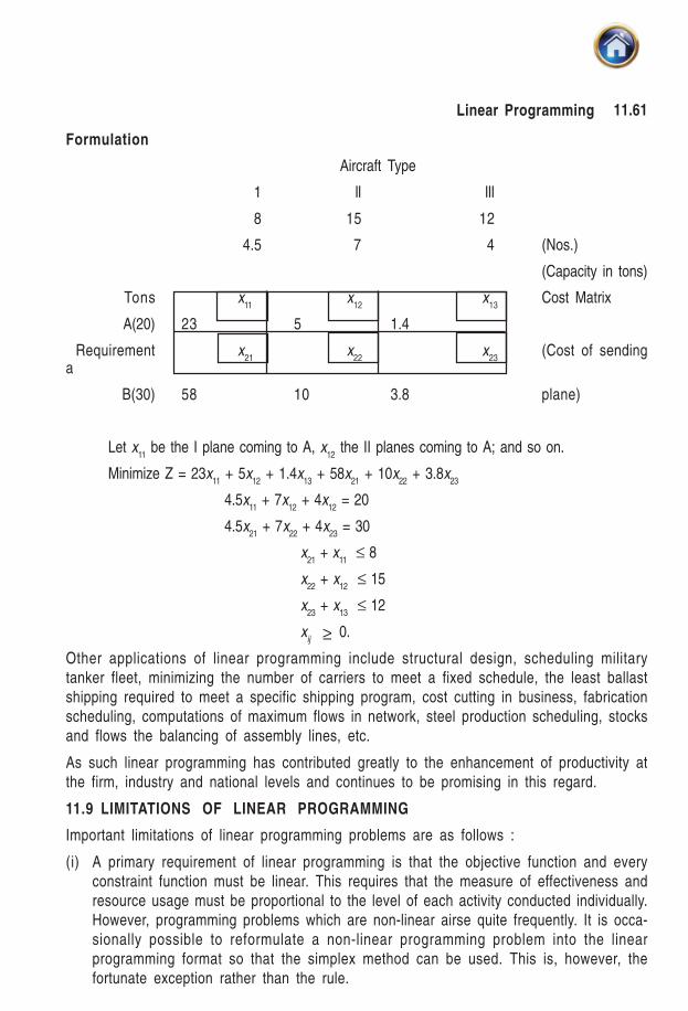
11.61Linear Programming
Formulation
Aircraft Type
1 II III
8 15 12
4.5 7 4 (Nos.)
(Capacity in tons)
Tons x11
x12
x13
Cost Matrix
A(20) 23 5 1.4
Requirement x21
x22
x23
(Cost of sendinga
B(30) 58 10 3.8 plane)
Let x11
be the I plane coming to A, x12
the II planes coming to A; and so on.
Minimize Z = 23x11
+ 5x12
+ 1.4x13
+ 58x21
+ 10x22
+ 3.8x23
4.5x11
+ 7x12
+ 4x12
= 20
4.5x21
+ 7x22
+ 4x23
= 30
x21
+ x11
≤ 8
x22
+ x12
≤ 15
x23
+ x13
≤ 12
xij ≥ 0.
Other applications of linear programming include structural design, scheduling militarytanker fleet, minimizing the number of carriers to meet a fixed schedule, the least ballastshipping required to meet a specific shipping program, cost cutting in business, fabricationscheduling, computations of maximum flows in network, steel production scheduling, stocksand flows the balancing of assembly lines, etc.
As such linear programming has contributed greatly to the enhancement of productivity atthe firm, industry and national levels and continues to be promising in this regard.
11.9 LIMITATIONS OF LINEAR PROGRAMMING
Important limitations of linear programming problems are as follows :
(i) A primary requirement of linear programming is that the objective function and everyconstraint function must be linear. This requires that the measure of effectiveness andresource usage must be proportional to the level of each activity conducted individually.However, programming problems which are non-linear airse quite frequently. It is occa-sionally possible to reformulate a non-linear programming problem into the linearprogramming format so that the simplex method can be used. This is, however, thefortunate exception rather than the rule.
11.62 Advanced Management Accounting
(ii) It may not be possible to solve those problems using linear programming, in which non-linerarity arises because of joint interactions between some of the activities regardingthe total measure of effectiveness or total usage of some resource. Hence linear pro-gramming problem requires that the total measure of effectiveness and total resourceusage resulting from the joint performance of the activities must equal the respectivesums of these quantities resulting from each activity being performed individually.
In some situations, it may not be true. For example, consider a situation where by aproduct is produced with the scrap material from the primary product. The materialwould still have to be procured if only one of the two products were produced. However,the total material requirements if both products are produced is less than the sum ofrequirements is each were produced individually. It may not be possible to handle suchsituation with linear programming problems.
(iii) In linear programming problem, fractional values are permitted for the decisions vari-ables. However, many decision problems require that the solution for decision variableshould be obtained in non-fractional values. Rounding-off the values obtained by linearprogramming techniques may not result into an optimal solution in such cases.
(iv) In linear programming problem, coefficients in the objective function and the constraintequations must be completely known and they should not change during the period ofstudy i.e. they should be known constraints. In practical situation, it may not be possibleto state all coefficients in the objective function and constraints with certainity. Further-more, these coefficients may actually be random variables, each with an underlyingprobablility distribution for the values. Such problems cannot be solved using linearprogramming.
SUMMARY
Linear Programming: The method of maximising (or minimising) a linear function of
several variables (called objective function) subject to the condition that the variables are
non negative and satisfy a set of linear equations and / or in equations (called linear constraints)
hence called linear programming.
It involves three steps:
1. To identify the objective function as a linear function of its variables and state all the
limitation on resources as linear equation and / or in equations (constraints) – This is
called a linear programming problem.
2. To use mathematical techniques to find all possible set or values of the variables
(unknowns), satisfying the constraints. This is called a set of feasible solution.
3. To select the particular set of values of the variables obtained in step 2 above that lead
to our objective pr maximum profit or least cost etc – This is called Optimum solution
of the Linear programming problem.
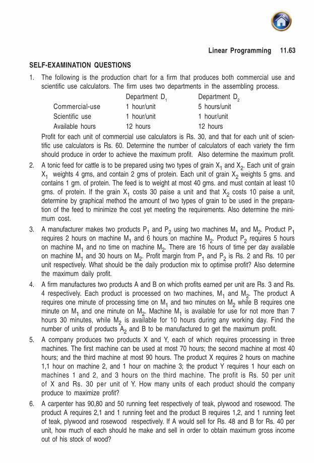
11.63Linear Programming
SELF-EXAMINATION QUESTIONS
1. The following is the production chart for a firm that produces both commercial use andscientific use calculators. The firm uses two departments in the assembling process.
Department D1
Department D2
Commercial-use 1 hour/unit 5 hours/unit
Scientific use 1 hour/unit 1 hour/unit
Available hours 12 hours 12 hours
Profit for each unit of commercial use calculators is Rs. 30, and that for each unit of scien-tific use calculators is Rs. 60. Determine the number of calculators of each variety the firmshould produce in order to achieve the maximum profit. Also determine the maximum profit.
2. A tonic feed for cattle is to be prepared using two types of grain X1 and X2. Each unit of grainX1 weights 4 gms, and contain 2 gms of protein. Each unit of grain X2 weights 5 gms. andcontains 1 gm. of protein. The feed is to weight at most 40 gms. and must contain at least 10gms. of protein. If the grain X1 costs 30 paise a unit and that X2 costs 10 paise a unit,determine by graphical method the amount of two types of grain to be used in the prepara-tion of the feed to minimize the cost yet meeting the requirements. Also determine the mini-mum cost.
3. A manufacturer makes two products P1 and P2 using two machines M1 and M2. Product P1requires 2 hours on machine M1 and 6 hours on machine M2. Product P2 requires 5 hourson machine M1 and no time on machine M2. There are 16 hours of time per day availableon machine M1 and 30 hours on M2. Profit margin from P1 and P2 is Rs. 2 and Rs. 10 perunit respectively. What should be the daily production mix to optimise profit? Also determinethe maximum daily profit.
4. A firm manufactures two products A and B on which profits earned per unit are Rs. 3 and Rs.4 respectively. Each product is processed on two machines, M1 and M2. The product Arequires one minute of processing time on M1 and two minutes on M2 while B requires oneminute on M1 and one minute on M2. Machine M1 is available for use for not more than 7hours 30 minutes, while M2 is available for 10 hours during any working day. Find thenumber of units of products A2 and B to be manufactured to get the maximum profit.
5. A company produces two products X and Y, each of which requires processing in threemachines. The first machine can be used at most 70 hours; the second machine at most 40hours; and the third machine at most 90 hours. The product X requires 2 hours on machine1,1 hour on machine 2, and 1 hour on machine 3; the product Y requires 1 hour each onmachines 1 and 2, and 3 hours on the third machine. The profit is Rs. 50 per unitof X and Rs. 30 per unit of Y. How many units of each product should the companyproduce to maximize profit?
6. A carpenter has 90,80 and 50 running feet respectively of teak, plywood and rosewood. Theproduct A requires 2,1 and 1 running feet and the product B requires 1,2, and 1 running feetof teak, plywood and rosewood respectively. If A would sell for Rs. 48 and B for Rs. 40 perunit, how much of each should he make and sell in order to obtain maximum gross incomeout of his stock of wood?
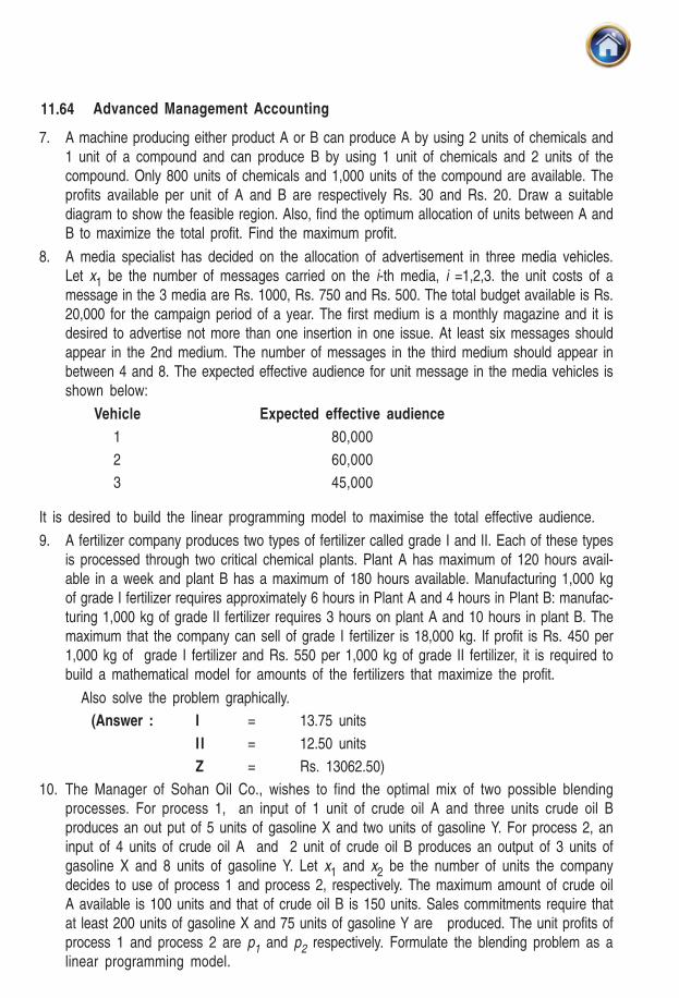
11.64 Advanced Management Accounting
7. A machine producing either product A or B can produce A by using 2 units of chemicals and1 unit of a compound and can produce B by using 1 unit of chemicals and 2 units of thecompound. Only 800 units of chemicals and 1,000 units of the compound are available. Theprofits available per unit of A and B are respectively Rs. 30 and Rs. 20. Draw a suitablediagram to show the feasible region. Also, find the optimum allocation of units between A andB to maximize the total profit. Find the maximum profit.
8. A media specialist has decided on the allocation of advertisement in three media vehicles.Let x1 be the number of messages carried on the i-th media, i =1,2,3. the unit costs of amessage in the 3 media are Rs. 1000, Rs. 750 and Rs. 500. The total budget available is Rs.20,000 for the campaign period of a year. The first medium is a monthly magazine and it isdesired to advertise not more than one insertion in one issue. At least six messages shouldappear in the 2nd medium. The number of messages in the third medium should appear inbetween 4 and 8. The expected effective audience for unit message in the media vehicles isshown below:
Vehicle Expected effective audience
1 80,000
2 60,000
3 45,000
It is desired to build the linear programming model to maximise the total effective audience.
9. A fertilizer company produces two types of fertilizer called grade I and II. Each of these typesis processed through two critical chemical plants. Plant A has maximum of 120 hours avail-able in a week and plant B has a maximum of 180 hours available. Manufacturing 1,000 kgof grade I fertilizer requires approximately 6 hours in Plant A and 4 hours in Plant B: manufac-turing 1,000 kg of grade II fertilizer requires 3 hours on plant A and 10 hours in plant B. Themaximum that the company can sell of grade I fertilizer is 18,000 kg. If profit is Rs. 450 per1,000 kg of grade I fertilizer and Rs. 550 per 1,000 kg of grade II fertilizer, it is required tobuild a mathematical model for amounts of the fertilizers that maximize the profit.
Also solve the problem graphically.
(Answer : I = 13.75 units
I I = 12.50 units
Z = Rs. 13062.50)
10. The Manager of Sohan Oil Co., wishes to find the optimal mix of two possible blendingprocesses. For process 1, an input of 1 unit of crude oil A and three units crude oil Bproduces an out put of 5 units of gasoline X and two units of gasoline Y. For process 2, aninput of 4 units of crude oil A and 2 unit of crude oil B produces an output of 3 units ofgasoline X and 8 units of gasoline Y. Let x1 and x2 be the number of units the companydecides to use of process 1 and process 2, respectively. The maximum amount of crude oilA available is 100 units and that of crude oil B is 150 units. Sales commitments require thatat least 200 units of gasoline X and 75 units of gasoline Y are produced. The unit profits ofprocess 1 and process 2 are p1 and p2 respectively. Formulate the blending problem as alinear programming model.

11.65Linear Programming
ANSWER TO SELF-EXAMINATION QUESTIONS
1. Commercial use calculator 0, Scientific use calculator 12; Max. profit = Rs. 720.
2. 5/3 units of X1 and 20/3 units of X
2; Min. Cost = 350/3 paise
3. 0 unit of P1 and 3.2 unit of P
2; Max Profit = Rs. 32.
4. 0 unit of A and 450 units of B.
5. 30 units of X and 10 units of Y.
6. 40 units of A and 10 units of B.
7. In figure 16, the shaded region is the feasible region.
Optimum allocation : 200 units of A and 400 units of B;
Max. Profit = Rs. 14,000.
8. Maximize Z = 80,000 x1 + 60,000 x2 + 45,000 x3
Subject to 1,000x1 + 750x2 + 500x3
≤ 20,000 (budget)
x1
≤ 12
x2
≥ 6
x3
≥ 4
x3 ≤ 8
x1, x
2, ≥ 0
9. Let x1 be the amount in 1,000 kg. of grade I fertilizer produced and x2 the amount in 1,000 kgof grade II produced. The total profit
Z = 450 x1 + 550x
2 is to be maximized
subject to constraints 6x1 + 3x
2 ≤ 120 Plant A Capacity
2x1 + 10x
2 ≤ 180 Plant B Capacity
x1 ≤ 18
x1, x
2 ≥ 0.
10. Maximize Z = P1 x1 + P2 x2
Subject to x1 + 4x2 ≤ 100
3x1 + 2x2 ≤ 150
5x1 + 3x2 ≥ 200
2x1 + 8x2 ≥ 75
x1, x
2 ≥ 0
(2 0 0 , 4 0 0 )(0 , 5 0 0 )
(4 0 0 , 3 0 0 )
(0 ,0 ) (4 0 0 ,0 )
2 x+
x=
80 0
12
x +x =
1
22
1000
X 2
X�
(0 , 8 0 0 )
⎤⎥⎦
Availability
Demand⎤⎥⎦