Automatic Synthesis of Microcontroller Assembly Code Through Linear Genetic Programming
247
Nadia Nedjah, Ajith Abraham, Luiza de Macedo Mourelle (Eds.) Genetic Systems Programming
-
Upload
independent -
Category
Documents
-
view
0 -
download
0
Transcript of Automatic Synthesis of Microcontroller Assembly Code Through Linear Genetic Programming

Nadia Nedjah, Ajith Abraham, Luiza de Macedo Mourelle (Eds.)
Genetic Systems Programming

Studies in Computational Intelligence, Volume 13
Editor-in-chiefProf. Janusz KacprzykSystems Research InstitutePolish Academy of Sciencesul. Newelska 601-447 WarsawPolandE-mail: [email protected]
Further volumes of this seriescan be found on our homepage:springer.com
Vol. 1. Tetsuya HoyaArtificial Mind System – Kernel MemoryApproach, 2005ISBN 3-540-26072-2
Vol. 2. Saman K. Halgamuge, Lipo Wang(Eds.)Computational Intelligence for Modellingand Prediction, 2005ISBN 3-540-26071-4
Vol. 3. Bozena KostekPerception-Based Data Processing inAcoustics, 2005ISBN 3-540-25729-2
Vol. 4. Saman K. Halgamuge, Lipo Wang(Eds.)Classification and Clustering for KnowledgeDiscovery, 2005ISBN 3-540-26073-0
Vol. 5. Da Ruan, Guoqing Chen, Etienne E.Kerre, Geert Wets (Eds.)Intelligent Data Mining, 2005ISBN 3-540-26256-3
Vol. 6. Tsau Young Lin, Setsuo Ohsuga,Churn-Jung Liau, Xiaohua Hu, ShusakuTsumoto (Eds.)Foundations of Data Mining and KnowledgeDiscovery, 2005ISBN 3-540-26257-1
Vol. 7. Bruno Apolloni, Ashish Ghosh, FerdaAlpaslan, Lakhmi C. Jain, Srikanta Patnaik(Eds.)Machine Learning and Robot Perception,2005ISBN 3-540-26549-X
Vol. 8. Srikanta Patnaik, Lakhmi C. Jain,Spyros G. Tzafestas, Germano Resconi,Amit Konar (Eds.)Innovations in Robot Mobility and Control,2005ISBN 3-540-26892-8
Vol. 9. Tsau Young Lin, Setsuo Ohsuga,Churn-Jung Liau, Xiaohua Hu (Eds.)Foundations and Novel Approaches in DataMining, 2005ISBN 3-540-28315-3
Vol. 10. Andrzej P. Wierzbicki, YoshiteruNakamoriCreative Space, 2005ISBN 3-540-28458-3
Vol. 11. Antoni LigêzaLogical Foundations for Rule-BasedSystems, 2006ISBN 3-540-29117-2
Vol. 13. Nadia Nedjah, Ajith Abraham,Luiza de Macedo Mourelle (Eds.)Genetic Systems Programming, 2006ISBN 3-540-29849-5

Nadia NedjahAjith AbrahamLuiza de Macedo Mourelle(Eds.)
Genetic SystemsProgrammingTheory and Experiences
ABC

Dr. Nadia NedjahDr. Luiza de Macedo MourelleFaculdade de EngenhariaUniversidade do Estadodo Rio de JaneiroRua Sao Francisco Xavier524, 20550-900 Maracana, Rio de JaneiroBrazilE-mail: [email protected]
Dr. Ajith AbrahamSchool for Computer Scienceand, EngineeringChung-Ang UniversityHeukseok-dong 221156-756 Seoul, KoreaRepublic of (South Korea)E-mail: [email protected]
Library of Congress Control Number: 2005936350
ISSN print edition: 1860-949XISSN electronic edition: 1860-9503ISBN-10 3-540-29849-5 Springer Berlin Heidelberg New YorkISBN-13 978-3-540-29849-6 Springer Berlin Heidelberg New York
This work is subject to copyright. All rights are reserved, whether the whole or part of the material isconcerned, specifically the rights of translation, reprinting, reuse of illustrations, recitation, broadcasting,reproduction on microfilm or in any other way, and storage in data banks. Duplication of this publicationor parts thereof is permitted only under the provisions of the German Copyright Law of September 9,1965, in its current version, and permission for use must always be obtained from Springer. Violations areliable for prosecution under the German Copyright Law.
Springer is a part of Springer Science+Business Mediaspringer.comc© Springer-Verlag Berlin Heidelberg 2006
Printed in The Netherlands
The use of general descriptive names, registered names, trademarks, etc. in this publication does not imply,even in the absence of a specific statement, that such names are exempt from the relevant protective lawsand regulations and therefore free for general use.
Typesetting: by the authors and TechBooks using a Springer LATEX macro package
Printed on acid-free paper SPIN: 11521433 89/TechBooks 5 4 3 2 1 0

Foreword
The editors of this volume, Nadia Nedjah, Ajith Abraham and Luiza deMacedo Mourelle, have done a superb job of assembling some of the mostinnovative and intriguing applications and additions to the methodology andtheory of genetic programming – an automatic programming technique thatstarts from a high-level statement of what needs to be done and automaticallycreates a computer program to solve the problem.
When the genetic algorithm first appeared in the 1960s and 1970s, it was anacademic curiosity that was primarily useful in understanding certain aspectsof how evolution worked in nature. In the 1980s, in tandem with the increasedavailability of computing power, practical applications of genetic and evolu-tionary computation first began to appear in specialized fields. In the 1990s,the relentless iteration of Moore’s law – which tracks the 100-fold increasein computational power every 10 years – enabled genetic and evolutionarycomputation to deliver the first results that were comparable and competitivewith the work of creative humans. As can be seen from the preface and tableof contents, the field has already begun the 21st century with a cornucopiaof applications, as well as additions to the methodology and theory, includingapplications to information security systems, compilers, data mining systems,stock market prediction systems, robotics, and automatic programming.
Looking forward three decades, there will be a 1,000,000-fold increase incomputational power. Given the impressive human-competitive results alreadydelivered by genetic programming and other techniques of evolutionary com-putation, the best is yet to come.
September 2005 Professor John R. Koza

Preface
Designing complex programs such as operating systems, compilers, filing sys-tems, data base systems, etc. is an old ever lasting research area. Geneticprogramming is a relatively new promising and growing research area. Amongother uses, it provides efficient tools to deal with hard problems by evolvingcreative and competitive solutions. Systems Programming is generally strewnwith such hard problems. This book is devoted to reporting innovative andsignificant progress about the contribution of genetic programming in systemsprogramming. The contributions of this book clearly demonstrate that geneticprogramming is very effective in solving hard and yet-open problems in sys-tems programming. Followed by an introductory chapter, in the remainingcontributed chapters, the reader can easily learn about systems where geneticprogramming can be applied successfully. These include but are not limitedto, information security systems (see Chapter 3), compilers (see Chapter 4),data mining systems (see Chapter 5), stock market prediction systems (seeChapter 6), robots (see Chapter 8) and automatic programming (see Chapters7 and 9).
In Chapter 1, which is entitled Evolutionary Computation: from GeneticAlgorithms to Genetic Programming, the authors introduce and review thedevelopment of the field of evolutionary computations from standard geneticalgorithms to genetic programming, passing by evolution strategies and evolu-tionary programming. The main differences among the different evolutionarycomputation techniques are also illustrated in this Chapter.
In Chapter 2, which is entitled Automatically Defined Functions in GeneExpression Programming, the author introduces the cellular system of GeneExpression Programming with Automatically Defined Functions (ADF) anddiscusses the importance of ADFs in Automatic Programming by compar-ing the performance of sophisticated learning systems with ADFs with muchsimpler ones without ADFs on a benchmark problem of symbolic regression.
VIII Preface
In Chapter 3, which is entitled Evolving Intrusion Detection Systems, theauthors present an Intrusion Detection System (IDS), which is a program thatanalyzes what happens or has happened during an execution and tries to findindications that the computer has been misused. An IDS does not eliminatethe use of preventive mechanism but it works as the last defensive mechanismin securing the system. The authors also evaluate the performances of twoGenetic Programming techniques for IDS namely Linear Genetic Program-ming (LGP) and Multi-Expression Programming (MEP). They compare theobtained results with some machine learning techniques like Support VectorMachines (SVM) and Decision Trees (DT). The authors claim that empiri-cal results clearly show that GP techniques could play an important role indesigning real time intrusion detection systems.
In Chapter 4, which is entitled Evolutionary Pattern Matching Using Ge-netic Programming, the authors apply GP to the hard problem of engineeringpattern matching automata for non-sequential pattern set, which is almostalways the case in functional programming. They engineer good traversal or-ders that allow one to design an efficient adaptive pattern-matchers that visitnecessary positions only. The authors claim that doing so the evolved pat-tern matching automata improves time and space requirements of pattern-matching as well as the termination properties of term evaluation.
In Chapter 5, which is entitled Genetic Programming in Data Modelling,the author demonstrates some abilities of Genetic Programming (GP) in DataModelling (DM). The author shows that GP can make data collected in largedatabases more useful and understandable. The author concentrates on math-ematical modelling, classification, prediction and modelling of time series.
In Chapter 6, which is entitled Stock Market Modeling Using Genetic Pro-gramming Ensembles, the authors introduce and use two Genetic Program-ming (GP) techniques: Multi-Expression Programming (MEP) and Linear Ge-netic Programming (LGP) for the prediction of two stock indices. They com-pare the performance of the GP techniques with an artificial neural networktrained using Levenberg-Marquardt algorithm and Takagi-Sugeno neuro-fuzzymodel. As a case study, the authors consider Nasdaq-100 index of NasdaqStock Market and the S&P CNX NIFTY stock index as test data. Based onthe empirical results obtained the authors conclude that Genetic Program-ming techniques are promising methods for stock prediction. Finally, theyformulate an ensemble of these two techniques using a multiobjective evolu-tionary algorithm and claim that results reached by ensemble of GP techniquesare better than the results obtained by each GP technique individually.
In Chapter 7, which is entitled Evolutionary Digital Circuit Design Us-ing Genetic Programming, the authors study two different circuit encodingsused for digital circuit evolution. The first approach is based on genetic pro-gramming, wherein digital circuits consist of their data flow based specifica-tions. In this approach, individuals are internally represented by the abstracttrees/DAG of the corresponding circuit specifications. In the second approach,digital circuits are thought of as a map of rooted gates. So individuals are

Preface IX
represented by two-dimensional arrays of cells. The authors compare the im-pact of both individual representations on the evolution process of digitalcircuits. The authors reach the conclusion that employing either of these ap-proaches yields circuits of almost the same characteristics in terms of spaceand response time. However, the evolutionary process is much shorter withthe second linear encoding.
In Chapter 8, which is entitled Evolving Complex Robotic Behaviors UsingGenetic Programming, the author reviews different methods for evolving com-plex robotic behaviors. The methods surveyed use two different approaches:The first one introduces hierarchy into GP by using library of proceduresor new primitive functions and the second one uses GP to evolve the build-ing modules of robot controller hierarchy. The author comments on includingpractical issues of evolution as well as comparison between the two approaches.
In Chapter 9, which is entitled Automatic Synthesis of Microcontroller As-sembly Code Through Linear Genetic Programming, the authors focus on thepotential of linear genetic programming in the automatic synthesis of micro-controller assembly language programs. For them, these programs implementstrategies for time-optimal or sub-optimal control of the system to be con-trolled, based on mathematical modeling through dynamic equations. Theyalso believe that within this application class, the best model is the one usedin linear genetic programming, in which each chromosome is represented byan instruction list. The authors find the synthesis of programs that implementoptimal-time control strategies for microcontrollers, directly in assembly lan-guage, as an attractive alternative that overcomes the difficulties presentedby the conventional design of optimal control systems. This chapter widensthe perspective of broad usage of genetic programming in automatic control.
We are very much grateful to the authors of this volume and to the re-viewers for their tremendous service by critically reviewing the chapters. Theeditors would like also to thank Prof. Janusz Kacprzyk, the editor-in-chiefof the Studies in Computational Intelligence Book Series and Dr. ThomasDitzinger, Springer Verlag, Germany for the editorial assistance and excellentcooperative collaboration to produce this important scientific work. We hopethat the reader will share our excitement to present this volume on GeneticSystems Programming and will find it useful.
Brazil Nadia NedjahAugust 2005 Ajith Abraham
Luiza M. Mourelle

Contents
1 Evolutionary Computation: from Genetic Algorithmsto Genetic ProgrammingAjith Abraham, Nadia Nedjah, Luiza de Macedo Mourelle . . . . . . . . . . . . . 11.1 Introduction . . . . . . . . . . . . . . . . . . . . . . . . . . . . . . . . . . . . . . . . . . . . . . . 2
1.1.1 Advantages of Evolutionary Algorithms . . . . . . . . . . . . . . . . . . . 31.2 Genetic Algorithms . . . . . . . . . . . . . . . . . . . . . . . . . . . . . . . . . . . . . . . . . 3
1.2.1 Encoding and Decoding . . . . . . . . . . . . . . . . . . . . . . . . . . . . . . . . . 41.2.2 Schema Theorem and Selection Strategies . . . . . . . . . . . . . . . . . 51.2.3 Reproduction Operators . . . . . . . . . . . . . . . . . . . . . . . . . . . . . . . . 6
1.3 Evolution Strategies . . . . . . . . . . . . . . . . . . . . . . . . . . . . . . . . . . . . . . . . 91.3.1 Mutation in Evolution Strategies . . . . . . . . . . . . . . . . . . . . . . . . . 91.3.2 Crossover (Recombination) in Evolution Strategies . . . . . . . . . 101.3.3 Controling the Evolution . . . . . . . . . . . . . . . . . . . . . . . . . . . . . . . . 10
1.4 Evolutionary Programming . . . . . . . . . . . . . . . . . . . . . . . . . . . . . . . . . . 111.5 Genetic Programming . . . . . . . . . . . . . . . . . . . . . . . . . . . . . . . . . . . . . . . 12
1.5.1 Computer Program Encoding . . . . . . . . . . . . . . . . . . . . . . . . . . . . 131.5.2 Reproduction of Computer Programs . . . . . . . . . . . . . . . . . . . . . 14
1.6 Variants of Genetic Programming . . . . . . . . . . . . . . . . . . . . . . . . . . . . . 151.6.1 Linear Genetic Programming . . . . . . . . . . . . . . . . . . . . . . . . . . . . 161.6.2 Gene Expression Programming (GEP) . . . . . . . . . . . . . . . . . . . . 161.6.3 Multi Expression Programming . . . . . . . . . . . . . . . . . . . . . . . . . . 171.6.4 Cartesian Genetic Programming . . . . . . . . . . . . . . . . . . . . . . . . . 181.6.5 Traceless Genetic Programming ( TGP) . . . . . . . . . . . . . . . . . . 181.6.6 Grammatical Evolution . . . . . . . . . . . . . . . . . . . . . . . . . . . . . . . . . 191.6.7 Genetic Algorithm for Deriving Software (GADS) . . . . . . . . . . 19
1.7 Summary . . . . . . . . . . . . . . . . . . . . . . . . . . . . . . . . . . . . . . . . . . . . . . . . . . 19References . . . . . . . . . . . . . . . . . . . . . . . . . . . . . . . . . . . . . . . . . . . . . . . . . . . . . . 19

XII Contents
2 Automatically Defined Functionsin Gene Expression ProgrammingCandida Ferreira . . . . . . . . . . . . . . . . . . . . . . . . . . . . . . . . . . . . . . . . . . . . . . . . . 212.1 Genetic Algorithms: Historical Background . . . . . . . . . . . . . . . . . . . . 21
2.1.1 Genetic Algorithms . . . . . . . . . . . . . . . . . . . . . . . . . . . . . . . . . . . . 222.1.2 Genetic Programming . . . . . . . . . . . . . . . . . . . . . . . . . . . . . . . . . . 222.1.3 Gene Expression Programming . . . . . . . . . . . . . . . . . . . . . . . . . . 25
2.2 The Architecture of GEP Individuals . . . . . . . . . . . . . . . . . . . . . . . . . . 272.2.1 Open Reading Frames and Genes . . . . . . . . . . . . . . . . . . . . . . . . 282.2.2 Structural Organization of Genes . . . . . . . . . . . . . . . . . . . . . . . . 302.2.3 Multigenic Chromosomes and Linking Functions . . . . . . . . . . . 32
2.3 Chromosome Domainsand Random Numerical Constants . . . . . . . . . . . . . . . . . . . . . . . . . . . . 33
2.4 Cells and the Creationof Automatically Defined Functions . . . . . . . . . . . . . . . . . . . . . . . . . . . 362.4.1 Homeotic Genes and the Cellular System of GEP . . . . . . . . . . 372.4.2 Multicellular Systems . . . . . . . . . . . . . . . . . . . . . . . . . . . . . . . . . . . 372.4.3 Incorporating Random Numerical Constants in ADFs . . . . . . 39
2.5 Analyzing the Importance of ADFsin Automatic Programming . . . . . . . . . . . . . . . . . . . . . . . . . . . . . . . . . . 402.5.1 General Settings . . . . . . . . . . . . . . . . . . . . . . . . . . . . . . . . . . . . . . . 402.5.2 Results without ADFs . . . . . . . . . . . . . . . . . . . . . . . . . . . . . . . . . . 422.5.3 Results with ADFs . . . . . . . . . . . . . . . . . . . . . . . . . . . . . . . . . . . . . 46
2.6 Summary . . . . . . . . . . . . . . . . . . . . . . . . . . . . . . . . . . . . . . . . . . . . . . . . . . 54References . . . . . . . . . . . . . . . . . . . . . . . . . . . . . . . . . . . . . . . . . . . . . . . . . . . . . . 55
3 Evolving Intrusion Detection SystemsAjith Abraham, Crina Grosan . . . . . . . . . . . . . . . . . . . . . . . . . . . . . . . . . . . . . 573.1 Introduction . . . . . . . . . . . . . . . . . . . . . . . . . . . . . . . . . . . . . . . . . . . . . . . 573.2 Intrusion Detection . . . . . . . . . . . . . . . . . . . . . . . . . . . . . . . . . . . . . . . . . 583.3 Related Research . . . . . . . . . . . . . . . . . . . . . . . . . . . . . . . . . . . . . . . . . . . 603.4 Evolving IDS Using Genetic Programming (GP) . . . . . . . . . . . . . . . . 63
3.4.1 Linear Genetic Programming (LGP) . . . . . . . . . . . . . . . . . . . . . . 633.4.2 Multi Expression Programming (MEP) . . . . . . . . . . . . . . . . . . . 643.4.3 Solution Representation . . . . . . . . . . . . . . . . . . . . . . . . . . . . . . . . . 643.4.4 Fitness Assignment . . . . . . . . . . . . . . . . . . . . . . . . . . . . . . . . . . . . 66
3.5 Machine Learning Techniques . . . . . . . . . . . . . . . . . . . . . . . . . . . . . . . . 663.5.1 Decision Trees . . . . . . . . . . . . . . . . . . . . . . . . . . . . . . . . . . . . . . . . . 673.5.2 Support Vector Machines (SVMs) . . . . . . . . . . . . . . . . . . . . . . . . 67
3.6 Experiment Setup and Results . . . . . . . . . . . . . . . . . . . . . . . . . . . . . . . 683.7 Conclusions . . . . . . . . . . . . . . . . . . . . . . . . . . . . . . . . . . . . . . . . . . . . . . . . 77References . . . . . . . . . . . . . . . . . . . . . . . . . . . . . . . . . . . . . . . . . . . . . . . . . . . . . . 77

Contents XIII
4 Evolutionary Pattern MatchingUsing Genetic ProgrammingNadia Nedjah, Luiza de Macedo Mourelle . . . . . . . . . . . . . . . . . . . . . . . . . . . 814.1 Introduction . . . . . . . . . . . . . . . . . . . . . . . . . . . . . . . . . . . . . . . . . . . . . . . 824.2 Preliminary Notation and Terminology . . . . . . . . . . . . . . . . . . . . . . . . 834.3 Adaptive Pattern Matching . . . . . . . . . . . . . . . . . . . . . . . . . . . . . . . . . . 86
4.3.1 Constructing Adaptive Automata . . . . . . . . . . . . . . . . . . . . . . . . 874.3.2 Example of Adaptive Automaton Construction . . . . . . . . . . . . 89
4.4 Heuristics for Good Traversal Orders . . . . . . . . . . . . . . . . . . . . . . . . . . 904.4.1 Inspecting Indexes First . . . . . . . . . . . . . . . . . . . . . . . . . . . . . . . . 904.4.2 Selecting Partial Indexes . . . . . . . . . . . . . . . . . . . . . . . . . . . . . . . . 904.4.3 A Good Traversal Order . . . . . . . . . . . . . . . . . . . . . . . . . . . . . . . . 91
4.5 Genetically-Programmed Matching Automata . . . . . . . . . . . . . . . . . . 924.5.1 Encoding of adaptive matching automata . . . . . . . . . . . . . . . . . 934.5.2 Decoding of Traversal Orders . . . . . . . . . . . . . . . . . . . . . . . . . . . . 944.5.3 Genetic Operators . . . . . . . . . . . . . . . . . . . . . . . . . . . . . . . . . . . . . 944.5.4 Fitness function . . . . . . . . . . . . . . . . . . . . . . . . . . . . . . . . . . . . . . . 99
4.6 Comparative Results . . . . . . . . . . . . . . . . . . . . . . . . . . . . . . . . . . . . . . . . 1014.7 Summary . . . . . . . . . . . . . . . . . . . . . . . . . . . . . . . . . . . . . . . . . . . . . . . . . . 102References . . . . . . . . . . . . . . . . . . . . . . . . . . . . . . . . . . . . . . . . . . . . . . . . . . . . . . 103
5 Genetic Programming in Data ModellingHalina Kwasnicka, Ewa Szpunar-Huk . . . . . . . . . . . . . . . . . . . . . . . . . . . . . . . 1055.1 Introduction . . . . . . . . . . . . . . . . . . . . . . . . . . . . . . . . . . . . . . . . . . . . . . . 1055.2 Genetic Programming in Mathematical Modelling . . . . . . . . . . . . . . 106
5.2.1 Adaptation of GP to Mathematical Modelling . . . . . . . . . . . . . 1075.2.2 An educational Example – the Hybrid of Genetic
Programming and Genetic Algorithm . . . . . . . . . . . . . . . . . . . . . 1085.2.3 General Remarks . . . . . . . . . . . . . . . . . . . . . . . . . . . . . . . . . . . . . . 113
5.3 Decision Models for Classification Tasks . . . . . . . . . . . . . . . . . . . . . . . 1145.3.1 Adaptation of GP to Clasification Task . . . . . . . . . . . . . . . . . . . 1155.3.2 An Example of Classification Rules Discovering using GP . . . 1175.3.3 Used Algorithm . . . . . . . . . . . . . . . . . . . . . . . . . . . . . . . . . . . . . . . . 1175.3.4 General Remarks . . . . . . . . . . . . . . . . . . . . . . . . . . . . . . . . . . . . . . 120
5.4 GP for Prediction Task and Time Series Odelling . . . . . . . . . . . . . . . 1205.4.1 Adaptation of GP to Prediction Task . . . . . . . . . . . . . . . . . . . . . 1215.4.2 Adaptation of GP to Prediction Tasks . . . . . . . . . . . . . . . . . . . . 1225.4.3 Hybrid GP and GA to Develope Solar Cycle’s Model . . . . . . . 1255.4.4 General Remarks . . . . . . . . . . . . . . . . . . . . . . . . . . . . . . . . . . . . . . 127
5.5 Summary . . . . . . . . . . . . . . . . . . . . . . . . . . . . . . . . . . . . . . . . . . . . . . . . . . 129References . . . . . . . . . . . . . . . . . . . . . . . . . . . . . . . . . . . . . . . . . . . . . . . . . . . . . . 129

XIV Contents
6 Stock Market ModelingUsing Genetic Programming EnsemblesCrina Grosan, Ajith Abraham . . . . . . . . . . . . . . . . . . . . . . . . . . . . . . . . . . . . . 1316.1 Introduction . . . . . . . . . . . . . . . . . . . . . . . . . . . . . . . . . . . . . . . . . . . . . . . 1316.2 Modeling Stock Market Prediction . . . . . . . . . . . . . . . . . . . . . . . . . . . . 1326.3 Intelligent Paradigms . . . . . . . . . . . . . . . . . . . . . . . . . . . . . . . . . . . . . . . 134
6.3.1 Multi Expression Programming (MEP) . . . . . . . . . . . . . . . . . . . 1346.3.2 Linear Genetic Programming (LGP) . . . . . . . . . . . . . . . . . . . . . . 1356.3.3 Artificial Neural Network (ANN) . . . . . . . . . . . . . . . . . . . . . . . . . 1366.3.4 Neuro-Fuzzy System. . . . . . . . . . . . . . . . . . . . . . . . . . . . . . . . . . . . 138
6.4 Ensemble of GP Techniques . . . . . . . . . . . . . . . . . . . . . . . . . . . . . . . . . . 1386.4.1 Nondominated Sorting Genetic Algorithm II (NSGA II) . . . . 139
6.5 Experiment Results . . . . . . . . . . . . . . . . . . . . . . . . . . . . . . . . . . . . . . . . . 1406.5.1 Parameter Settings . . . . . . . . . . . . . . . . . . . . . . . . . . . . . . . . . . . . . 1406.5.2 Comparisons of Results Obtained by Intelligent Paradigms . . 143
6.6 Summary . . . . . . . . . . . . . . . . . . . . . . . . . . . . . . . . . . . . . . . . . . . . . . . . . . 144References . . . . . . . . . . . . . . . . . . . . . . . . . . . . . . . . . . . . . . . . . . . . . . . . . . . . . . 144
7 Evolutionary Digital Circuit DesignUsing Genetic ProgrammingNadia Nedjah, Luiza de Macedo Mourelle . . . . . . . . . . . . . . . . . . . . . . . . . . . 1477.1 Introduction . . . . . . . . . . . . . . . . . . . . . . . . . . . . . . . . . . . . . . . . . . . . . . . 1477.2 Principles of Evolutionary Hardware Design . . . . . . . . . . . . . . . . . . . . 1487.3 Circuit Designs = Programs . . . . . . . . . . . . . . . . . . . . . . . . . . . . . . . . . 152
7.3.1 Encoding . . . . . . . . . . . . . . . . . . . . . . . . . . . . . . . . . . . . . . . . . . . . . 1527.3.2 Genetic Operators . . . . . . . . . . . . . . . . . . . . . . . . . . . . . . . . . . . . . 153
7.4 Circuit Designs = Schematics . . . . . . . . . . . . . . . . . . . . . . . . . . . . . . . . 1557.4.1 Encoding . . . . . . . . . . . . . . . . . . . . . . . . . . . . . . . . . . . . . . . . . . . . . 1557.4.2 Genetic Operators . . . . . . . . . . . . . . . . . . . . . . . . . . . . . . . . . . . . . 158
7.5 Result Comparison . . . . . . . . . . . . . . . . . . . . . . . . . . . . . . . . . . . . . . . . . 1617.6 Conclusion . . . . . . . . . . . . . . . . . . . . . . . . . . . . . . . . . . . . . . . . . . . . . . . . . 171References . . . . . . . . . . . . . . . . . . . . . . . . . . . . . . . . . . . . . . . . . . . . . . . . . . . . . . 171
8 Evolving Complex Robotic BehaviorsUsing Genetic ProgrammingMichael Botros . . . . . . . . . . . . . . . . . . . . . . . . . . . . . . . . . . . . . . . . . . . . . . . . . . 1738.1 Introducing Khepera Robot . . . . . . . . . . . . . . . . . . . . . . . . . . . . . . . . . 1738.2 Evolving Complex Behaviors
by Introducing Hierarchy to GP . . . . . . . . . . . . . . . . . . . . . . . . . . . . . . 1758.2.1 Genetic Programming with Subroutine Library . . . . . . . . . . . . 1768.2.2 Neural Networks and the Control of Mobile Robots . . . . . . . . 1798.2.3 Using Neural Networks as Elements of the Function Set . . . . . 1818.2.4 Comments . . . . . . . . . . . . . . . . . . . . . . . . . . . . . . . . . . . . . . . . . . . . 182
8.3 Evolving Complex Behaviorsby Introducing Hierarchy to the Controller . . . . . . . . . . . . . . . . . . . . . 184

Contents XV
8.3.1 Subsumption Architecture . . . . . . . . . . . . . . . . . . . . . . . . . . . . . . 1848.3.2 Action Selection Architecture . . . . . . . . . . . . . . . . . . . . . . . . . . . . 1858.3.3 Using GP to Evolve Modules of Subsumption Architecture . . 1868.3.4 Using GP to Evolve Modules
of Action Selection Architecture . . . . . . . . . . . . . . . . . . . . . . . . . 1888.4 Comments . . . . . . . . . . . . . . . . . . . . . . . . . . . . . . . . . . . . . . . . . . . . . . . . . 1898.5 Summary . . . . . . . . . . . . . . . . . . . . . . . . . . . . . . . . . . . . . . . . . . . . . . . . . . 190References . . . . . . . . . . . . . . . . . . . . . . . . . . . . . . . . . . . . . . . . . . . . . . . . . . . . . . 191
9 Automatic Synthesis of Microcontroller Assembly CodeThrough Linear Genetic ProgrammingDouglas Mota Dias, Marco Aurelio C. Pacheco, Jose F. M. Amaral . . . . 1939.1 Introduction . . . . . . . . . . . . . . . . . . . . . . . . . . . . . . . . . . . . . . . . . . . . . . . 1949.2 Survey on Genetic Programming Applied to Synthesis of Assembly195
9.2.1 JB Language . . . . . . . . . . . . . . . . . . . . . . . . . . . . . . . . . . . . . . . . . . 1959.2.2 VRM-M . . . . . . . . . . . . . . . . . . . . . . . . . . . . . . . . . . . . . . . . . . . . . . 1969.2.3 AIMGP. . . . . . . . . . . . . . . . . . . . . . . . . . . . . . . . . . . . . . . . . . . . . . . 1969.2.4 GEMS . . . . . . . . . . . . . . . . . . . . . . . . . . . . . . . . . . . . . . . . . . . . . . . . 1979.2.5 Discussion . . . . . . . . . . . . . . . . . . . . . . . . . . . . . . . . . . . . . . . . . . . . 197
9.3 Design with Microcontrollers . . . . . . . . . . . . . . . . . . . . . . . . . . . . . . . . . 1989.3.1 Microcontrollers . . . . . . . . . . . . . . . . . . . . . . . . . . . . . . . . . . . . . . . 1989.3.2 Time-Optimal Control . . . . . . . . . . . . . . . . . . . . . . . . . . . . . . . . . . 199
9.4 Microcontroller Platform . . . . . . . . . . . . . . . . . . . . . . . . . . . . . . . . . . . . 2009.5 Linear Genetic Programming . . . . . . . . . . . . . . . . . . . . . . . . . . . . . . . . . 201
9.5.1 Evolution of Assembly Language Programs . . . . . . . . . . . . . . . . 2029.6 System for Automatic Synthesis
of Microcontroller Assembly . . . . . . . . . . . . . . . . . . . . . . . . . . . . . . . . . 2029.6.1 Evolutionary Kernel . . . . . . . . . . . . . . . . . . . . . . . . . . . . . . . . . . . . 2029.6.2 Plant Simulator . . . . . . . . . . . . . . . . . . . . . . . . . . . . . . . . . . . . . . . . 2069.6.3 Microcontroller Simulator . . . . . . . . . . . . . . . . . . . . . . . . . . . . . . . 2069.6.4 A/D and D/A Converters . . . . . . . . . . . . . . . . . . . . . . . . . . . . . . . 2079.6.5 Overview . . . . . . . . . . . . . . . . . . . . . . . . . . . . . . . . . . . . . . . . . . . . . 207
9.7 Case Studies . . . . . . . . . . . . . . . . . . . . . . . . . . . . . . . . . . . . . . . . . . . . . . . 2089.7.1 Cart Centering . . . . . . . . . . . . . . . . . . . . . . . . . . . . . . . . . . . . . . . . 2089.7.2 Inverted Pendulum . . . . . . . . . . . . . . . . . . . . . . . . . . . . . . . . . . . . . 218
9.8 Summary . . . . . . . . . . . . . . . . . . . . . . . . . . . . . . . . . . . . . . . . . . . . . . . . . . 225References . . . . . . . . . . . . . . . . . . . . . . . . . . . . . . . . . . . . . . . . . . . . . . . . . . . . . . 226
Reviewer List . . . . . . . . . . . . . . . . . . . . . . . . . . . . . . . . . . . . . . . . . . . . . . . . . . 233

List of Figures
1.1 Flow chart of an evolutionary algorithm . . . . . . . . . . . . . . . . . . . . . 21.2 Flow chart of basic genetic algorithm iteration . . . . . . . . . . . . . . . 41.3 Roulette wheel selection . . . . . . . . . . . . . . . . . . . . . . . . . . . . . . . . . . . 71.4 Types of crossover operators . . . . . . . . . . . . . . . . . . . . . . . . . . . . . . . 81.5 A simple tree structure of GP . . . . . . . . . . . . . . . . . . . . . . . . . . . . . . 131.6 Illustration of crossover operator . . . . . . . . . . . . . . . . . . . . . . . . . . . 141.7 Illustration of mutation operator in GP . . . . . . . . . . . . . . . . . . . . . 152.1 Tree crossover in Genetic Programming. The arrows indicate
the crossover points. . . . . . . . . . . . . . . . . . . . . . . . . . . . . . . . . . . . . . . 232.2 Tree mutation in Genetic Programming . . . . . . . . . . . . . . . . . . . . . 242.3 Permutation in Genetic Programming . . . . . . . . . . . . . . . . . . . . . . . 242.4 Illustration of a hypothetical event of point mutation in
Genetic Programming . . . . . . . . . . . . . . . . . . . . . . . . . . . . . . . . . . . . . 252.5 The flowchart of Gene Expression Programming. . . . . . . . . . . . . . 272.6 Expression of GEP genes as sub-ETs . . . . . . . . . . . . . . . . . . . . . . . 332.7 The overall structure of an S-expression . . . . . . . . . . . . . . . . . . . . . 362.8 Expression of a unicellular system with three Automatically
Defined Functions . . . . . . . . . . . . . . . . . . . . . . . . . . . . . . . . . . . . . . . . 382.9 Expression of a multicellular system with three Automatically
Defined Functions . . . . . . . . . . . . . . . . . . . . . . . . . . . . . . . . . . . . . . . . 392.10 Expression of a multicellular system with Automatically
Defined Functions containing random numerical constants. . . . . 413.1 Network protected by an IDS . . . . . . . . . . . . . . . . . . . . . . . . . . . . . . 593.2 A generic intrusion detection model . . . . . . . . . . . . . . . . . . . . . . . . . 603.3 Relation between accuracy and number of generations: (a)
normal mode (b) probe attacks . . . . . . . . . . . . . . . . . . . . . . . . . . . . . 713.4 Relation between accuracy and number of generations: (c)
DoS attacks (d) U2R attacks . . . . . . . . . . . . . . . . . . . . . . . . . . . . . . 713.5 Relation between accuracy and number of generations: (e)
R2L attacks . . . . . . . . . . . . . . . . . . . . . . . . . . . . . . . . . . . . . . . . . . . . . 72

XVIII List of Figures
3.6 Relationship between the best result obtained for trainingdata set and the average of results obtained for training /testdata: (a) normal mode (b) probe attacks . . . . . . . . . . . . . . . . . . . . 72
3.7 Relationship between the best result obtained for trainingdata set and the average of results obtained for training /testdata: (c) DoS attacks (d) U2R attacks . . . . . . . . . . . . . . . . . . . . . . 73
3.8 Relationship between the best result obtained for trainingdata set and the average of results obtained for training /testdata: (e) R2L attacks . . . . . . . . . . . . . . . . . . . . . . . . . . . . . . . . . . . . . 73
3.9 Growth of program codes for normal mode . . . . . . . . . . . . . . . . . . 743.10 Growth of program codes for probe attacks . . . . . . . . . . . . . . . . . . 743.11 Growth of program codes for DOS attacks . . . . . . . . . . . . . . . . . . . 753.12 Growth of program codes for U2R attacks . . . . . . . . . . . . . . . . . . . 753.13 Growth of program codes for R2L attacks . . . . . . . . . . . . . . . . . . . 764.1 An adaptive automaton for 1 : fωaω, 2 : fωωa, 3 : fωgωωgωω 894.2 Simplified representation of the adaptive automaton of Figure
4.1 or corresponding traversal order . . . . . . . . . . . . . . . . . . . . . . . . . 934.3 Internal representation of the traversal order of Figure 4.2 . . . . . 944.4 Another possible traversal order for Π . . . . . . . . . . . . . . . . . . . . . . 954.5 An adaptive automaton for 1 : fωaω, 2 : fωωa, 3 : fωgωωgωω 954.6 Single-point crossover of traversal orders . . . . . . . . . . . . . . . . . . . . 964.7 Double-point crossover of traversal orders . . . . . . . . . . . . . . . . . . . 974.8 Mutation of non-final state to another non-final state . . . . . . . . . 984.9 Mutation of non-final state to a final state . . . . . . . . . . . . . . . . . . . 984.10 Mutation of final state to another final state . . . . . . . . . . . . . . . . . 995.1 An examplary tree in GP and the coded expression . . . . . . . . . . . 1075.2 An example of crossover in TA . . . . . . . . . . . . . . . . . . . . . . . . . . . . . 1135.3 The scheme of the GP in conjunction with GA used as TA
algorithms . . . . . . . . . . . . . . . . . . . . . . . . . . . . . . . . . . . . . . . . . . . . . . . 1135.4 An exemplary tree in GESTIN algorithm . . . . . . . . . . . . . . . . . . . . 1235.5 The scheme of GESTIN algorithm . . . . . . . . . . . . . . . . . . . . . . . . . . 1235.6 Changes in Sun activity . . . . . . . . . . . . . . . . . . . . . . . . . . . . . . . . . . . 1255.7 Data preprocessing . . . . . . . . . . . . . . . . . . . . . . . . . . . . . . . . . . . . . . . 1265.8 Sunspot approximation – short-time test . . . . . . . . . . . . . . . . . . . . 1275.9 The best approximation of sunspots – short-time test . . . . . . . . . 1275.10 The best approximation of sunspots – long-time test . . . . . . . . . . 1286.1 Training and test data sets for Nasdaq-100 Index . . . . . . . . . . . . . 1336.2 Training and test data sets for NIFTY index . . . . . . . . . . . . . . . . . 1336.3 Architecture of ANFIS . . . . . . . . . . . . . . . . . . . . . . . . . . . . . . . . . . . . 1387.1 VHDL data-flow specification for the circuit whose behaviour
is given in Table 7.2 . . . . . . . . . . . . . . . . . . . . . . . . . . . . . . . . . . . . . . 1517.2 Chromosome with respect to the first encoding . . . . . . . . . . . . . . . 1527.3 Single-point crossover of circuit specifications . . . . . . . . . . . . . . . . 1537.4 Double-point crossover of circuit specifications . . . . . . . . . . . . . . . 1547.5 The impact of the crossover operator for circuit specifications . . 154

List of Figures XIX
7.6 Operand node mutation for circuit specification . . . . . . . . . . . . . . 1567.7 Operator node mutation for circuit specification . . . . . . . . . . . . . . 1567.8 Chromosome with respect to the second encoding . . . . . . . . . . . . 1577.9 Four-point crossover of circuit schematics . . . . . . . . . . . . . . . . . . . . 1587.10 Triple-point crossover of circuit schematics . . . . . . . . . . . . . . . . . . 1597.11 Double-point crossover of circuit schematics . . . . . . . . . . . . . . . . . 1597.12 Single-point crossover of circuit schematics . . . . . . . . . . . . . . . . . . 1607.13 The impact of the crossover operator for circuit schematics . . . . 1617.14 Mutation of circuit schematics . . . . . . . . . . . . . . . . . . . . . . . . . . . . . 1627.15 Encoding 1: evolved circuit for the benchmark a . . . . . . . . . . . . . . 1637.16 Encoding 1: Data-Flow specification of the evolved circuit for
the benchmark a . . . . . . . . . . . . . . . . . . . . . . . . . . . . . . . . . . . . . . . . . 1647.17 Encoding 1: evolved circuit for the benchmark b . . . . . . . . . . . . . . 1647.18 Encoding 1: Data-flow specifcation of the evolved circuit for
the benchmark b . . . . . . . . . . . . . . . . . . . . . . . . . . . . . . . . . . . . . . . . . 1647.19 Encoding 1: evolved circuit for the benchmark c in Table 7.6 . . . 1657.20 Encoding 1: Data-flow specification of the evolved circuit for
the benchmark c . . . . . . . . . . . . . . . . . . . . . . . . . . . . . . . . . . . . . . . . . 1657.21 Encoding 1: evolved circuit for the benchmark d . . . . . . . . . . . . . . 1667.22 Encoding 1: Data-flow specification of the evolved circuit for
the benchmark d . . . . . . . . . . . . . . . . . . . . . . . . . . . . . . . . . . . . . . . . . 1667.23 Encoding 2: evolved circuit for the benchmark a in Table 7.6 . . . 1677.24 Encoding 2: Data-flow specification of the evolved circuit for
the benchmark a . . . . . . . . . . . . . . . . . . . . . . . . . . . . . . . . . . . . . . . . . 1677.25 Encoding 2: evolved circuit for the benchmark b in Table 7.6 . . . 1677.26 Encoding 2: Data-flow specification of the evolved circuit for
the benchmark b . . . . . . . . . . . . . . . . . . . . . . . . . . . . . . . . . . . . . . . . . 1687.27 Encoding 2: evolved circuit for the benchmark c in Table 7.6 . . . 1687.28 Encoding 2: Data-flow specification of the evolved circuit for
the benchmark c . . . . . . . . . . . . . . . . . . . . . . . . . . . . . . . . . . . . . . . . . 1687.29 Encoding 2: evolved circuit for the benchmark d in Table 7.6 . . . 1697.30 Encoding 2: Data-flow specification of the evolved circuit for
the benchmark d . . . . . . . . . . . . . . . . . . . . . . . . . . . . . . . . . . . . . . . . . 1697.31 Fitness comparison . . . . . . . . . . . . . . . . . . . . . . . . . . . . . . . . . . . . . . . 1707.32 Performance Comparison . . . . . . . . . . . . . . . . . . . . . . . . . . . . . . . . . . 1708.1 Miniature mobile robot Khepera (with permission of K-team) . . 1748.2 The position of the eight sensors on the robot (with permission
of K-team) . . . . . . . . . . . . . . . . . . . . . . . . . . . . . . . . . . . . . . . . . . . . . . 1748.3 Example of program tree in conventional GP and GP
implementing ADF . . . . . . . . . . . . . . . . . . . . . . . . . . . . . . . . . . . . . . . 1768.4 Environment of the experiment . . . . . . . . . . . . . . . . . . . . . . . . . . . . 1788.5 Model of a single neuron . . . . . . . . . . . . . . . . . . . . . . . . . . . . . . . . . . 1798.6 Artificial neural network with three layers . . . . . . . . . . . . . . . . . . . 1808.7 Subsumption architecture . . . . . . . . . . . . . . . . . . . . . . . . . . . . . . . . . 1848.8 Action selection architecture . . . . . . . . . . . . . . . . . . . . . . . . . . . . . . . 185

XX List of Figures
8.9 Action selection architecture with tree-like structure . . . . . . . . . . 1868.10 Khepera robot with the gripper mounted on the top of it
(with permission of K-team) . . . . . . . . . . . . . . . . . . . . . . . . . . . . . . . 1879.1 Structure of a program individual in AIMGP . . . . . . . . . . . . . . . . 1979.2 The GEMS crossover and mutation process . . . . . . . . . . . . . . . . . . 1989.3 Block diagram of the system . . . . . . . . . . . . . . . . . . . . . . . . . . . . . . . 2039.4 Crossover of two individuals . . . . . . . . . . . . . . . . . . . . . . . . . . . . . . . 2049.5 Mutation on an individual . . . . . . . . . . . . . . . . . . . . . . . . . . . . . . . . . 2059.6 Operation of the synthesis system . . . . . . . . . . . . . . . . . . . . . . . . . . 2089.7 The cart-centering problem controlled by a PIC . . . . . . . . . . . . . . 2099.8 Flowchart of the evaluation function for the cart-centering
problem . . . . . . . . . . . . . . . . . . . . . . . . . . . . . . . . . . . . . . . . . . . . . . . . . 2129.9 Evolution of the cart-centering problem, without control over
the length of the individuals . . . . . . . . . . . . . . . . . . . . . . . . . . . . . . . 2159.10 Evolution of the cart-centering problem, with control over the
length of the individuals . . . . . . . . . . . . . . . . . . . . . . . . . . . . . . . . . . . 2169.11 The inverted pendulum problem controlled by a PIC . . . . . . . . . . 2199.12 Evolution of the inverted pendulum problem, with control
over the length of the individuals. . . . . . . . . . . . . . . . . . . . . . . . . . . 222

List of Tables
2.1 Settings for the sextic polynomial problem using a unigenicsystem with (ugGEP-RNC) and without (ugGEP) randomnumerical constants . . . . . . . . . . . . . . . . . . . . . . . . . . . . . . . . . . . . . . . 43
2.2 Settings for the sextic polynomial problem using a multigenicsystem with (mgGEP-RNC) and without (mgGEP)random numerical constants . . . . . . . . . . . . . . . . . . . . . . . . . . . . . . . 45
2.3 Settings and performance for the sextic polynomial problemusing a unicellular system encoding 1, 2, 3, and 4 ADFs . . . . . . . 48
2.4 Settings and performance for the sextic polynomial problemusing a unicellular system encoding 1, 2, 3, and 4 ADFs withrandom numerical constants . . . . . . . . . . . . . . . . . . . . . . . . . . . . . . . 50
2.5 Settings and performance for the sextic polynomial problemusing a multicellular system encoding 1, 2, 3, and 4 ADFs . . . . . 51
2.6 Settings and performance for the sextic polynomial problemusing a multicellular system encoding 1, 2, 3, and 4 ADFswith random numerical constants . . . . . . . . . . . . . . . . . . . . . . . . . . . 53
3.1 Variables for intrusion detection data set . . . . . . . . . . . . . . . . . . . . 693.2 Parameter settings for LGP. . . . . . . . . . . . . . . . . . . . . . . . . . . . . . . . 703.3 Parameters used by MEP . . . . . . . . . . . . . . . . . . . . . . . . . . . . . . . . . 763.4 Functions evolved by MEP . . . . . . . . . . . . . . . . . . . . . . . . . . . . . . . . 763.5 Performance comparison . . . . . . . . . . . . . . . . . . . . . . . . . . . . . . . . . . 774.1 Space and time requirements for miscellaneous benchmarks . . . . 1025.1 Sample of test functions and number of generations needed to
find that function by the algorithm . . . . . . . . . . . . . . . . . . . . . . . . . 1115.2 The result given by GP+GA for different number of additional
variables . . . . . . . . . . . . . . . . . . . . . . . . . . . . . . . . . . . . . . . . . . . . . . . . 1115.3 Obtained result in Minerals classification [16] . . . . . . . . . . . . . . . . 1195.4 Indexes in outer nodes . . . . . . . . . . . . . . . . . . . . . . . . . . . . . . . . . . . . 1225.5 Results of 10 different strategies for one learning and three
testing time periods of different value of WIG index . . . . . . . . . . 1246.1 Values of parameters used by MEP . . . . . . . . . . . . . . . . . . . . . . . . . 141

XXII List of Tables
6.2 Performance measures obtained by MEP or population sizes . . . 1416.3 Performance measures obtained by MEP for different
chromosome lengths . . . . . . . . . . . . . . . . . . . . . . . . . . . . . . . . . . . . . . 1426.4 LGP parameter settings . . . . . . . . . . . . . . . . . . . . . . . . . . . . . . . . . . . 1426.5 Parameters values used by NSGAII for ensembling MEP and
LGP . . . . . . . . . . . . . . . . . . . . . . . . . . . . . . . . . . . . . . . . . . . . . . . . . . . . 1426.6 Results obtained by intelligent paradigms for Nasdaq and
Nifty test data . . . . . . . . . . . . . . . . . . . . . . . . . . . . . . . . . . . . . . . . . . . 1437.1 Gates symbols, number of gate-equivalent . . . . . . . . . . . . . . . . . . . 1497.2 Truth table of the circuit whose schematics are given in Fig. 7.1 1517.3 Performance comparison of the specification crossover variations1557.4 Chromosome for the circuit of Fig. 7.8 . . . . . . . . . . . . . . . . . . . . . . 1577.5 Performance comparison of the schematics crossover variations . 1617.6 Truth table of the circuit used as benchmarks to compare
both encoding methodologies . . . . . . . . . . . . . . . . . . . . . . . . . . . . . . 1637.7 Number of gate-equivalent and generations required to evolve
the circuits presented . . . . . . . . . . . . . . . . . . . . . . . . . . . . . . . . . . . . . 1697.8 Performance comparison of the impact of the studied encodings 1709.1 Taxonomy over the evolution of assembly language programs. . . 1969.2 Instruction subset of the PIC18F452 . . . . . . . . . . . . . . . . . . . . . . . . 2019.3 Summary of the evolutionary experiment with the
cart-centering problem . . . . . . . . . . . . . . . . . . . . . . . . . . . . . . . . . . . . 2139.4 Summary of the evolutionary experiment with the inverted
pendulum problem . . . . . . . . . . . . . . . . . . . . . . . . . . . . . . . . . . . . . . . 221

1
Evolutionary Computation: from GeneticAlgorithms to Genetic Programming
Ajith Abraham1, Nadia Nedjah2 and Luiza de Macedo Mourelle3
1 School of Computer Science and Engineering Chung-Ang University 410,2nd Engineering Building 221, Heukseok-dong,Dongjak-gu Seoul 156-756, [email protected], http://www.ajith.softcomputing.net
2 Department of Electronics Engineering and Telecommunications,Engineering Faculty,State University of Rio de Janeiro,Rua Sao Francisco Xavier, 524, Sala 5022-D,Maracana, Rio de Janeiro, [email protected], http://www.eng.uerj.br/~nadia
3 Department of System Engineering and Computation,Engineering Faculty,State University of Rio de Janeiro,Rua Sao Francisco Xavier, 524, Sala 5022-D,Maracana, Rio de Janeiro, [email protected], http://www.eng.uerj.br/~ldmm
Evolutionary computation, offers practical advantages to the researcher facingdifficult optimization problems. These advantages are multi-fold, including thesimplicity of the approach, its robust response to changing circumstance, itsflexibility, and many other facets. The evolutionary approach can be appliedto problems where heuristic solutions are not available or generally lead tounsatisfactory results. As a result, evolutionary computation have receivedincreased interest, particularly with regards to the manner in which they maybe applied for practical problem solving.
In this chapter, we review the development of the field of evolutionary com-putations from standard genetic algorithms to genetic programming, passingby evolution strategies and evolutionary programming. For each of these orien-tations, we identify the main differences from the others. We also, describe themost popular variants of genetic programming. These include linear geneticprogramming (LGP), gene expression programming (GEP), multi-expressonprogramming (MEP), Cartesian genetic programming (CGP), traceless ge-netic programming (TGP), gramatical evolution (GE) and genetic glgorithmfor deriving software (GADS).
A. Abraham et al.: Evolutionary Computation: from Genetic Algorithms to Genetic Program-ming, Studies in Computational Intelligence (SCI) 13, 1–20 (2006)www.springerlink.com c© Springer-Verlag Berlin Heidelberg 2006

2 Ajith Abraham et al.
1.1 Introduction
In nature, evolution is mostly determined by natural selection or differentindividuals competing for resources in the environment. Those individualsthat are better are more likely to survive and propagate their genetic material.The encoding for genetic information (genome) is done in a way that admitsasexual reproduction which results in offspring that are genetically identicalto the parent. Sexual reproduction allows some exchange and re-ordering ofchromosomes, producing offspring that contain a combination of informationfrom each parent. This is the recombination operation, which is often referredto as crossover because of the way strands of chromosomes cross over duringthe exchange. The diversity in the population is achieved by mutation.
Evolutionary algorithms are ubiquitous nowadays, having been success-fully applied to numerous problems from different domains, including op-timization, automatic programming, machine learning, operations research,bioinformatics, and social systems. In many cases the mathematical function,which describes the problem is not known and the values at certain parame-ters are obtained from simulations. In contrast to many other optimizationtechniques an important advantage of evolutionary algorithms is they cancope with multi-modal functions.
Usually grouped under the term evolutionary computation [1] or evolu-tionary algorithms, we find the domains of genetic algorithms [9], evolutionstrategies [17, 19], evolutionary programming [5] and genetic programming[11]. They all share a common conceptual base of simulating the evolutionof individual structures via processes of selection, mutation, and reproduc-tion. The processes depend on the perceived performance of the individualstructures as defined by the problem.
A population of candidate solutions (for the optimization task to be solved)is initialized. New solutions are created by applying reproduction operators(mutation and/or crossover). The fitness (how good the solutions are) of theresulting solutions are evaluated and suitable selection strategy is then appliedto determine which solutions will be maintained into the next generation. Theprocedure is then iterated and is illustrated in Fig. 1.1.
Replacement
Reproduction
SelectionPopulation Parents
Offspring
Fig. 1.1. Flow chart of an evolutionary algorithm

1 Evolutionary Computation: from GA to GP 3
1.1.1 Advantages of Evolutionary Algorithms
A primary advantage of evolutionary computation is that it is conceptuallysimple. The procedure may be written as difference equation (1.1):
x[t + 1] = s(v(x[t])) (1.1)
where x[t] is the population at time t under a representation x, v is arandom variation operator, and s is the selection operator [6].
Other advantages can be listed as follows:
• Evolutionary algorithm performance is representation independent, in con-trast with other numerical techniques, which might be applicable for onlycontinuous values or other constrained sets.
• Evolutionary algorithms offer a framework such that it is comparably easyto incorporate prior knowledge about the problem. Incorporating such in-formation focuses the evolutionary search, yielding a more efficient explo-ration of the state space of possible solutions.
• Evolutionary algorithms can also be combined with more traditional op-timization techniques. This may be as simple as the use of a gradientminimization used after primary search with an evolutionary algorithm(for example fine tuning of weights of a evolutionary neural network), or itmay involve simultaneous application of other algorithms (e.g., hybridiz-ing with simulated annealing or tabu search to improve the efficiency ofbasic evolutionary search).
• The evaluation of each solution can be handled in parallel and only selec-tion (which requires at least pair wise competition) requires some serialprocessing. Implicit parallelism is not possible in many global optimizationalgorithms like simulated annealing and Tabu search.
• Traditional methods of optimization are not robust to dynamic changes inproblem the environment and often require a complete restart in order toprovide a solution (e.g., dynamic programming). In contrast, evolutionaryalgorithms can be used to adapt solutions to changing circumstance.
• Perhaps the greatest advantage of evolutionary algorithms comes fromthe ability to address problems for which there are no human experts.Although human expertise should be used when it is available, it oftenproves less than adequate for automating problem-solving routines.
1.2 Genetic Algorithms
A typical flowchart of a Genetic Algorithm (GA) is depicted in Fig. 1.2. Oneiteration of the algorithm is referred to as a generation. The basic GA isvery generic and there are many aspects that can be implemented differentlyaccording to the problem (For instance, representation of solution or chromo-somes, type of encoding, selection strategy, type of crossover and mutation

4 Ajith Abraham et al.
operators, etc.) In practice, GAs are implemented by having arrays of bits orcharacters to represent the chromosomes. The individuals in the populationthen go through a process of simulated evolution. Simple bit manipulationoperations allow the implementation of crossover, mutation and other opera-tions. The number of bits for every gene (parameter) and the decimal range inwhich they decode are usually the same but nothing precludes the utilizationof a different number of bits or range for every gene.
Initialize Population
Evaluate Fitness
Solution
Found?
End
Selection
Reproduction
yes
no
Fig. 1.2. Flow chart of basic genetic algorithm iteration
When compared to other evolutionary algorithms, one of the most im-portant GA feature is its focus on fixed-length character strings althoughvariable-length strings and other structures have been used.
1.2.1 Encoding and Decoding
In a typical application of GA’s, the given problem is transformed into a setof genetic characteristics (parameters to be optimized) that will survive in thebest possible manner in the environment. Example, if the task is to optimizethe function given in 1.2.
min f(x1, x2) = (x1 − 5)2 + (x2 − 2)2,−3 ≤ x1 ≤ 3, −8 ≤ x2 ≤ 8 (1.2)

1 Evolutionary Computation: from GA to GP 5
The parameters of the search are identified as x1 and x2, which are calledthe phenotypes in evolutionary algorithms. In genetic algorithms, the phe-notypes (parameters) are usually converted to genotypes by using a codingprocedure. Knowing the ranges of x1 and x2 each variable is to be representedusing a suitable binary string. This representation using binary coding makesthe parametric space independent of the type of variables used. The genotype(chromosome) should in some way contain information about solution, whichis also known as encoding. GA’s use a binary string encoding as shown below.
Chromosome A: 110110111110100110110Chromosome B: 110111101010100011110
Each bit in the chromosome strings can represent some characteristic ofthe solution. There are several types of encoding (example, direct integer orreal numbers encoding). The encoding depends directly on the problem.
Permutation encoding can be used in ordering problems, such as TravellingSalesman Problem (TSP) or task ordering problem. In permutation encoding,every chromosome is a string of numbers, which represents number in a se-quence. A chromosome using permutation encoding for a 9 city TSP problemwill look like as follows:
Chromosome A: 4 5 3 2 6 1 7 8 9Chromosome B: 8 5 6 7 2 3 1 4 9
Chromosome represents order of cities, in which salesman will visit them.Special care is to taken to ensure that the strings represent real sequencesafter crossover and mutation. Floating-point representation is very useful fornumeric optimization (example: for encoding the weights of a neural network).It should be noted that in many recent applications more sophisticated geno-types are appearing (example: chromosome can be a tree of symbols, or is acombination of a string and a tree, some parts of the chromosome are notallowed to evolve etc.)
1.2.2 Schema Theorem and Selection Strategies
Theoretical foundations of evolutionary algorithms can be partially explainedby schema theorem [9], which relies on the concept of schemata. Schemataare templates that partially specify a solution (more strictly, a solution in thegenotype space). If genotypes are strings built using symbols from an alphabetA, schemata are strings whose symbols belong to A ∪ ∗. This extra-symbol* must be interpreted as a wildcard, being loci occupied by it called undefined.A chromosome is said to match a schema if they agree in the defined positions.
For example, the string 10011010 matches the schemata 1******* and**011*** among others, but does not match *1*11*** because they differ inthe second gene (the first defined gene in the schema). A schema can be viewed

6 Ajith Abraham et al.
as a hyper-plane in a k-dimensional space representing a set of solutions withcommon properties. Obviously, the number of solutions that match a schemaH depend on the number of defined positions in it. Another related concept isthe defining-length of a schema, defined as the distance between the first andthe last defined positions in it. The GA works by allocating strings to bestschemata exponentially through successive generations, being the selectionmechanism the main responsible for this behaviour. On the other hand thecrossover operator is responsible for exploring new combinations of the presentschemata in order to get the fittest individuals. Finally the purpose of themutation operator is to introduce fresh genotypic material in the population.
1.2.3 Reproduction Operators
Individuals for producing offspring are chosen using a selection strategy afterevaluating the fitness value of each individual in the selection pool. Eachindividual in the selection pool receives a reproduction probability dependingon its own fitness value and the fitness value of all other individuals in theselection pool. This fitness is used for the actual selection step afterwards.Some of the popular selection schemes are discussed below.
Roulette Wheel Selection
The simplest selection scheme is roulette-wheel selection, also called stochasticsampling with replacement. This technique is analogous to a roulette wheelwith each slice proportional in size to the fitness. The individuals are mappedto contiguous segments of a line, such that each individual’s segment is equalin size to its fitness. A random number is generated and the individual whosesegment spans the random number is selected. The process is repeated un-til the desired number of individuals is obtained. As illustrated in Fig. 1.3,chromosome1 has the highest probability for being selected since it has thehighest fitness.
Tournament Selection
In tournament selection a number of individuals is chosen randomly from thepopulation and the best individual from this group is selected as parent. Thisprocess is repeated as often as individuals to choose. These selected parentsproduce uniform at random offspring. The tournament size will often dependon the problem, population size etc. The parameter for tournament selectionis the tournament size. Tournament size takes values ranging from 2 – numberof individuals in population.

1 Evolutionary Computation: from GA to GP 7
Chromosome1
Chromosome2
Chromosome3
Chromosome4
Chromosome5
Fig. 1.3. Roulette wheel selection
Elitism
When creating new population by crossover and mutation, we have a bigchance that we will lose the best chromosome. Elitism is name of the methodthat first copies the best chromosome (or a few best chromosomes) to newpopulation. The rest is done in classical way. Elitism can very rapidly increaseperformance of GA, because it prevents losing the best-found solution.
Genetic Operators
Crossover and mutation are two basic operators of GA. Performance of GAvery much depends on the genetic operators. Type and implementation of op-erators depends on encoding and also on the problem. There are many wayshow to do crossover and mutation. In this section we will demonstrate someof the popular methods with some examples and suggestions how to do it fordifferent encoding schemes.
Crossover. It selects genes from parent chromosomes and creates a new off-spring. The simplest way to do this is to choose randomly some crossoverpoint and everything before this point is copied from the first parent andthen everything after a crossover point is copied from the second parent. Asingle point crossover is illustrated as follows (| is the crossover point):
Chromosome A: 11111 | 00100110110Chromosome B: 10011 | 11000011110
Offspring A: 11111 | 11000011110Offspring B: 10011 | 00100110110
As illustrated in Fig. 1.4, there are several crossover techniques. In a uni-form crossover bits are randomly copied from the first or from the second

8 Ajith Abraham et al.
Uniform crossover
offspring1 offspring2
parent1 parent2
Two-point crossover
offspring1 offspring2
parent1 parent2
Single-point crossover
offspring1 offspring2
parent1 parent2
Fig. 1.4. Types of crossover operators
parent. Specific crossover made for a specific problem can improve the GAperformance.
Mutation. After crossover operation, mutation takes place. Mutation changesrandomly the new offspring. For binary encoding mutation is performed bychanging a few randomly chosen bits from 1 to 0 or from 0 to 1. Mutationdepends on the encoding as well as the crossover. For example when we areencoding permutations, mutation could be exchanging two genes. A simplemutation operation is illustrated as follows:
Chromosome A: 1101111000011110Chromosome B: 1101100100110110

1 Evolutionary Computation: from GA to GP 9
Offspring A: 1100111000011110Offspring B: 1101101100110110
For many optimization problems there may be multiple, equal, or unequaloptimal solutions. Sometimes a simple GA cannot maintain stable populationsat different optima of such functions. In the case of unequal optimal solutions,the population invariably converges to the global optimum. Niching helps tomaintain subpopulations near global and local optima. A niche is viewed asan organism’s environment and a species as a collection of organisms withsimilar features. Niching helps to maintain subpopulations near global andlocal optima by introducing a controlled competition among different solutionsnear every local optimal region. Niching is achieved by a sharing function,which creates subdivisions of the environment by degrading an organism’sfitness proportional to the number of other members in its neighbourhood.The amount of sharing contributed by each individual into its neighbour isdetermined by their proximity in the decoded parameter space (phenotypicsharing) based on a distance measure.
1.3 Evolution Strategies
Evolution Strategy (ES) was developed by Rechenberg [17] at Technical Uni-versity, Berlin. ES tend to be used for empirical experiments that are difficultto model mathematically. The system to be optimized is actually constructedand ES is used to find the optimal parameter settings. Evolution strategiesmerely concentrate on translating the fundamental mechanisms of biologicalevolution for technical optimization problems. The parameters to be optimizedare often represented by a vector of real numbers (object parameters – op).Another vector of real numbers defines the strategy parameters (sp) whichcontrols the mutation of the objective parameters. Both object and strategicparameters form the data-structure for a single individual. A population P ofn individuals could be described as P = (c1, c2, . . . , cn−1, cn), where the ithchromosome ci is defined as ci = (op, sp) with op = (o1, o2, ..., on−1, on) andsp = (s1, s2, ..., sn−1, sn).
1.3.1 Mutation in Evolution Strategies
The mutation operator is defined as component wise addition of normal dis-tributed random numbers. Both the objective parameters and the strategyparameters of the chromosome are mutated. A mutant’s object-parametersvector is calculated as op(mut) = op + N0(sp), where N0(si) is the Gaussiandistribution of mean-value 0 and standard deviation si. Usually the strategyparameters mutation step size is done by adapting the standard deviation si.For instance, this may be done by sp(mut) = (s1 × A1, s2 × A2, . . . , sn−1 ×An−1, sn×An), where Ai is randomly chosen from α or 1/α depending on the

10 Ajith Abraham et al.
value of equally distributed random variable E of [0,1] with Ai = α if E < 0.5and Ai = 1/α if E ≥ 0.5. The parameter α is usually referred to as strategyparameters adaptation value.
1.3.2 Crossover (Recombination) in Evolution Strategies
For two chromosomes c1 = (op(c1), sp(c1)) and c2 = (op(c2), sp(c2)) thecrossover operator is defined R(c1, c2) = c = (op, sp) with op(i) = (op(c1),i|op(c2), i) and sp(i) = (sp(c1), i|sp(c2), i). By defining op(i) and sp(i) = (x|y)a value is randomly assigned for either x or y (50% selection probability forx and y).
1.3.3 Controling the Evolution
Let P be the number of parents in generation 1 and let C be the number ofchildren in generation i. There are basically four different types of evolutionstrategies: P , C, P +C, P/R,C and P/R+C as discussed below. They mainlydiffer in how the parents for the next generation are selected and the usage ofcrossover operators.
P, C Strategy
The P parents produce C children using mutation. Fitness values are calcu-lated for each of the C children and the best P children become next gener-ation parents. The best individuals of C children are sorted by their fitnessvalue and the first P individuals are selected to be next generation parents(C ≥ P ).
P + C Strategy
The P parents produce C children using mutation. Fitness values are calcu-lated for each of the C children and the best P individuals of both parents andchildren become next generation parents. Children and parents are sorted bytheir fitness value and the first P individuals are selected to be next generationparents.
P/R, C Strategy
The P parents produce C children using mutation and crossover. Fitnessvalues are calculated for each of the C children and the best P children becomenext generation parents. The best individuals of C children are sorted by theirfitness value and the first P individuals are selected to be next generationparents (C ≥ P ). Except the usage of crossover operator this is exactly thesame as P,C strategy.
1 Evolutionary Computation: from GA to GP 11
P/R + C Strategy
The P parents produce C children using mutation and recombination. Fitnessvalues are calculated for each of the C children and the best P individualsof both parents and children become next generation parents. Children andparents are sorted by their fitness value and the first P individuals are selectedto be next generation parents. Except the usage of crossover operator this isexactly the same as P + C strategy.
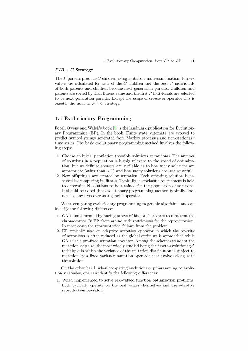
1.4 Evolutionary Programming
Fogel, Owens and Walsh’s book [5] is the landmark publication for Evolution-ary Programming (EP). In the book, Finite state automata are evolved topredict symbol strings generated from Markov processes and non-stationarytime series. The basic evolutionary programming method involves the follow-ing steps:
1. Choose an initial population (possible solutions at random). The numberof solutions in a population is highly relevant to the speed of optimiza-tion, but no definite answers are available as to how many solutions areappropriate (other than > 1) and how many solutions are just wasteful.
2. New offspring’s are created by mutation. Each offspring solution is as-sessed by computing its fitness. Typically, a stochastic tournament is heldto determine N solutions to be retained for the population of solutions.It should be noted that evolutionary programming method typically doesnot use any crossover as a genetic operator.
When comparing evolutionary programming to genetic algorithm, one canidentify the following differences:
1. GA is implemented by having arrays of bits or characters to represent thechromosomes. In EP there are no such restrictions for the representation.In most cases the representation follows from the problem.
2. EP typically uses an adaptive mutation operator in which the severityof mutations is often reduced as the global optimum is approached whileGA’s use a pre-fixed mutation operator. Among the schemes to adapt themutation step size, the most widely studied being the “meta-evolutionary”technique in which the variance of the mutation distribution is subject tomutation by a fixed variance mutation operator that evolves along withthe solution.
On the other hand, when comparing evolutionary programming to evolu-tion strategies, one can identify the following differences:
1. When implemented to solve real-valued function optimization problems,both typically operate on the real values themselves and use adaptivereproduction operators.

12 Ajith Abraham et al.
2. EP typically uses stochastic tournament selection while ES typically usesdeterministic selection.
3. EP does not use crossover operators while ES (P/R,C and P/R+C strate-gies) uses crossover. However the effectiveness of the crossover operatorsdepends on the problem at hand.
1.5 Genetic Programming
Genetic Programming (GP) technique provides a framework for automaticallycreating a working computer program from a high-level problem statement ofthe problem [11]. Genetic programming achieves this goal of automatic pro-gramming by genetically breeding a population of computer programs usingthe principles of Darwinian natural selection and biologically inspired opera-tions. The operations include most of the techniques discussed in the previoussections. The main difference between genetic programming and genetic al-gorithms is the representation of the solution. Genetic programming createscomputer programs in the LISP or scheme computer languages as the so-lution. LISP is an acronym for LISt Processor and was developed by JohnMcCarthy in the late 1950s [8]. Unlike most languages, LISP is usually usedas an interpreted language. This means that, unlike compiled languages, aninterpreter can process and respond directly to programs written in LISP. Themain reason for choosing LISP to implement GP is due to the advantage ofhaving the programs and data have the same structure, which could provideeasy means for manipulation and evaluation.
Genetic programming is the extension of evolutionary learning into thespace of computer programs. In GP the individual population members arenot fixed length character strings that encode possible solutions to the problemat hand, they are programs that, when executed, are the candidate solutionsto the problem. These programs are expressed in genetic programming asparse trees, rather than as lines of code. For example, the simple program“a + b ∗ f(4, a, c)” would be represented as shown in Fig. 1.5. The terminaland function sets are also important components of genetic programming.The terminal and function sets are the alphabet of the programs to be made.The terminal set consists of the variables (example, a,b and c in Fig. 1.5) andconstants (example, 4 in Fig. 1.5).
The most common way of writing down a function with two argumentsis the infix notation. That is, the two arguments are connected with theoperation symbol between them as a + b or a ∗ b. A different method isthe prefix notation. Here the operation symbol is written down first, fol-lowed by its required arguments as +ab or ∗ab. While this may be a bitmore difficult or just unusual for human eyes, it opens some advantages forcomputational uses. The computer language LISP uses symbolic expressions(or S-expressions) composed in prefix notation. Then a simple S-expressioncould be (operator, argument) where operator is the name of a function and

1 Evolutionary Computation: from GA to GP 13
+
a *
b f
4 a c
Fig. 1.5. A simple tree structure of GP
argument can be either a constant or a variable or either another symbolic ex-pression as (operator, argument(operator, argument)(operator, argument)).Generally speaking, GP procedure could be summarized as follows:
• Generate an initial population of random compositions of the functionsand terminals of the problem;
• Compute the fitness values of each individual in the population ;• Using some selection strategy and suitable reproduction operators produce
two offspring;• Procedure is iterated until the required solution is found or the termination
conditions have reached (specified number of generations).
1.5.1 Computer Program Encoding
A parse tree is a structure that grasps the interpretation of a computer pro-gram. Functions are written down as nodes, their arguments as leaves. Asubtree is the part of a tree that is under an inner node of this tree. If thistree is cut out from its parent, the inner node becomes a root node and thesubtree is a valid tree of its own.
There is a close relationship between these parse trees and S-expression;in fact these trees are just another way of writing down expressions. Whilefunctions will be the nodes of the trees (or the operators in the S-expressions)and can have other functions as their arguments, the leaves will be formedby terminals, that is symbols that may not be further expanded. Terminalscan be variables, constants or specific actions that are to be performed. Theprocess of selecting the functions and terminals that are needed or useful forfinding a solution to a given problem is one of the key steps in GP. Evaluation

14 Ajith Abraham et al.
of these structures is straightforward. Beginning at the root node, the valuesof all sub-expressions (or subtrees) are computed, descending the tree downto the leaves.
1.5.2 Reproduction of Computer Programs
The creation of an offspring from the crossover operation is accomplishedby deleting the crossover fragment of the first parent and then inserting thecrossover fragment of the second parent. The second offspring is produced ina symmetric manner. A simple crossover operation is illustrated in Fig. 1.6.In GP the crossover operation is implemented by taking randomly selectedsub trees in the individuals and exchanging them.
Fig. 1.6. Illustration of crossover operator
Mutation is another important feature of genetic programming. Two typesof mutations are commonly used. The simplest type is to replace a functionor a terminal by a function or a terminal respectively. In the second kind anentire subtree can replace another subtree. Fig. 1.7 explains the concept ofmutation.
GP requires data structures that are easy to handle and evaluate and ro-bust to structural manipulations. These are among the reasons why the class

1 Evolutionary Computation: from GA to GP 15
Fig. 1.7. Illustration of mutation operator in GP
of S-expressions was chosen to implement GP. The set of functions and termi-nals that will be used in a specific problem has to be chosen carefully. If theset of functions is not powerful enough, a solution may be very complex ornot to be found at all. Like in any evolutionary computation technique, thegeneration of first population of individuals is important for successful imple-mentation of GP. Some of the other factors that influence the performance ofthe algorithm are the size of the population, percentage of individuals thatparticipate in the crossover/mutation, maximum depth for the initial individ-uals and the maximum allowed depth for the generated offspring etc. Somespecific advantages of genetic programming are that no analytical knowledgeis needed and still could get accurate results. GP approach does scale with theproblem size. GP does impose restrictions on how the structure of solutionsshould be formulated.
1.6 Variants of Genetic Programming
Several variants of GP could be seen in the literature. Some of them are LinearGenetic Programming (LGP), Gene Expression Programming (GEP), MultiExpression Programming (MEP), Cartesian Genetic Programming (CGP),Traceless Genetic Programming (TGP) and Genetic Algorithm for DerivingSoftware (GADS).
16 Ajith Abraham et al.
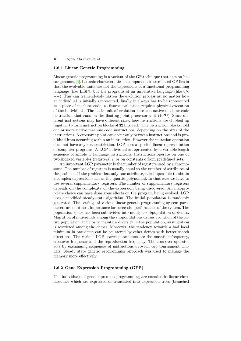
1.6.1 Linear Genetic Programming
Linear genetic programming is a variant of the GP technique that acts on lin-ear genomes [3]. Its main characteristics in comparison to tree-based GP lies inthat the evolvable units are not the expressions of a functional programminglanguage (like LISP), but the programs of an imperative language (like c/c++). This can tremendously hasten the evolution process as, no matter howan individual is initially represented, finally it always has to be representedas a piece of machine code, as fitness evaluation requires physical executionof the individuals. The basic unit of evolution here is a native machine codeinstruction that runs on the floating-point processor unit (FPU). Since dif-ferent instructions may have different sizes, here instructions are clubbed uptogether to form instruction blocks of 32 bits each. The instruction blocks holdone or more native machine code instructions, depending on the sizes of theinstructions. A crossover point can occur only between instructions and is pro-hibited from occurring within an instruction. However the mutation operationdoes not have any such restriction. LGP uses a specific linear representationof computer programs. A LGP individual is represented by a variable lengthsequence of simple C language instructions. Instructions operate on one ortwo indexed variables (registers) r, or on constants c from predefined sets.
An important LGP parameter is the number of registers used by a chromo-some. The number of registers is usually equal to the number of attributes ofthe problem. If the problem has only one attribute, it is impossible to obtaina complex expression such as the quartic polynomial. In that case we have touse several supplementary registers. The number of supplementary registersdepends on the complexity of the expression being discovered. An inappro-priate choice can have disastrous effects on the program being evolved. LGPuses a modified steady-state algorithm. The initial population is randomlygenerated. The settings of various linear genetic programming system para-meters are of utmost importance for successful performance of the system. Thepopulation space has been subdivided into multiple subpopulation or demes.Migration of individuals among the subpopulations causes evolution of the en-tire population. It helps to maintain diversity in the population, as migrationis restricted among the demes. Moreover, the tendency towards a bad localminimum in one deme can be countered by other demes with better searchdirections. The various LGP search parameters are the mutation frequency,crossover frequency and the reproduction frequency: The crossover operatoracts by exchanging sequences of instructions between two tournament win-ners. Steady state genetic programming approach was used to manage thememory more effectively
1.6.2 Gene Expression Programming (GEP)
The individuals of gene expression programming are encoded in linear chro-mosomes which are expressed or translated into expression trees (branched

1 Evolutionary Computation: from GA to GP 17
entities)[4]. Thus, in GEP, the genotype (the linear chromosomes) and thephenotype (the expression trees) are different entities (both structurally andfunctionally) that, nevertheless, work together forming an indivisible whole. Incontrast to its analogous cellular gene expression, GEP is rather simple. Themain players in GEP are only two: the chromosomes and the Expression Trees(ETs), being the latter the expression of the genetic information encoded inthe chromosomes. As in nature, the process of information decoding is calledtranslation. And this translation implies obviously a kind of code and a setof rules. The genetic code is very simple: a one-to-one relationship betweenthe symbols of the chromosome and the functions or terminals they repre-sent. The rules are also very simple: they determine the spatial organizationof the functions and terminals in the ETs and the type of interaction betweensub-ETs. GEP uses linear chromosomes that store expressions in breadth-firstform. A GEP gene is a string of terminal and function symbols. GEP genes arecomposed of a head and a tail. The head contains both function and terminalsymbols. The tail may contain terminal symbols only. For each problem thehead length (denoted h) is chosen by the user. The tail length (denoted by t)is evaluated by:
t = (n − 1)h + 1, (1.3)
where nis the number of arguments of the function with more arguments.GEP genes may be linked by a function symbol in order to obtain a fully
functional chromosome. GEP uses mutation, recombination and transposi-tion. GEP uses a generational algorithm. The initial population is randomlygenerated. The following steps are repeated until a termination criterion isreached: A fixed number of the best individuals enter the next generation(elitism). The mating pool is filled by using binary tournament selection. Theindividuals from the mating pool are randomly paired and recombined. Twooffspring are obtained by recombining two parents. The offspring are mutatedand they enter the next generation.
1.6.3 Multi Expression Programming
A GP chromosome generally encodes a single expression (computer program).A Multi Expression Programming (MEP) chromosome encodes several expres-sions [14]. The best of the encoded solution is chosen to represent the chromo-some. The MEP chromosome has some advantages over the single-expressionchromosome especially when the complexity of the target expression is notknown. This feature also acts as a provider of variable-length expressions.MEP genes are represented by substrings of a variable length. The numberof genes per chromosome is constant. This number defines the length of thechromosome. Each gene encodes a terminal or a function symbol. A gene thatencodes a function includes pointers towards the function arguments. Func-tion arguments always have indices of lower values than the position of thefunction itself in the chromosome.

18 Ajith Abraham et al.
The proposed representation ensures that no cycle arises while the chro-mosome is decoded (phenotypically transcripted). According to the proposedrepresentation scheme, the first symbol of the chromosome must be a terminalsymbol. In this way, only syntactically correct programs (MEP individuals)are obtained. The maximum number of symbols in MEP chromosome is givenby the formula:
Number of Symbols = (n + 1) × (Number of Genes − 1) + 1, (1.4)
where n is the number of arguments of the function with the greatest num-ber of arguments. The translation of a MEP chromosome into a computerprogram represents the phenotypic transcription of the MEP chromosomes.Phenotypic translation is obtained by parsing the chromosome top-down. Aterminal symbol specifies a simple expression. A function symbol specifiesa complex expression obtained by connecting the operands specified by theargument positions with the current function symbol.
Due to its multi expression representation, each MEP chromosome maybe viewed as a forest of trees rather than as a single tree, which is the case ofGenetic Programming.
1.6.4 Cartesian Genetic Programming
Cartesian Genetic Programming ( CGP) uses a network of nodes (indexedgraph) to achieve an input to output mapping [13]. Each node consists of anumber of inputs, these being used as parameters in a determined mathe-matical or logical function to create the node output. The functionality andconnectivity of the nodes are stored as a string of numbers (the genotype)and evolved to achieve the optimum mapping. The genotype is then mappedto an indexed graph that can be executed as a program.
In CGP there are very large number of genotypes that map to identi-cal genotypes due to the presence of a large amount of redundancy. Firstlythere is node redundancy that is caused by genes associated with nodes thatare not part of the connected graph representing the program. Another formof redundancy in CGP, also present in all other forms of GP is, functionalredundancy.
1.6.5 Traceless Genetic Programming ( TGP)
The main difference between Traceless Genetic Programming and GP is thatTGP does not explicitly store the evolved computer programs [15]. TGP isuseful when the trace (the way in which the results are obtained) between theinput and output is not important. TGP uses two genetic operators: crossoverand insertion. The insertion operator is useful when the population containsindividuals representing very complex expressions that cannot improve thesearch.

1 Evolutionary Computation: from GA to GP 19
1.6.6 Grammatical Evolution
Grammatical evolution [18] is a grammar-based, linear genome system. Ingrammatical evolution, the Backus Naur Form (BNF) specification of a lan-guage is used to describe the output produced by the system (a compilablecode fragment). Different BNF grammars can be used to produce code auto-matically in any language. The genotype is a string of eight-bit binary numbersgenerated at random and treated as integer values from 0 to 255. The phe-notype is a running computer program generated by a genotype-phenotypemapping process. The genotype-phenotype mapping in grammatical evolutionis deterministic because each individual is always mapped to the same pheno-type. In grammatical evolution, standard genetic algorithms are applied to thedifferent genotypes in a population using the typical crossover and mutationoperators.
1.6.7 Genetic Algorithm for Deriving Software (GADS)
Genetic algorithm for deriving software is a GP technique where the genotypeis distinct from the phenotype [16]. The GADS genotype is a list of integersrepresenting productions in a syntax. This is used to generate the phenotype,which is a program in the language defined by the syntax. Syntactically in-valid phenotypes cannot be generated, though there may be phenotypes withresidual nonterminals.
1.7 Summary
This chapter presented the biological motivation and fundamental aspects ofevolutionary algorithms and its constituents, namely genetic algorithm, evo-lution strategies, evolutionary programming and genetic programming. Mostpopular variants of genetic programming are introduced. Important advan-tages of evolutionary computation while compared to classical optimizationtechniques are also discussed.
References
1. Abraham, A., Evolutionary Computation, In: Handbook for Measurement, Sys-tems Design, Peter Sydenham and Richard Thorn (Eds.), John Wiley and SonsLtd., London, ISBN 0-470-02143-8, pp. 920–931, 2005. 2
2. Back, T., Evolutionary algorithms in theory and practice: Evolution Strategies,Evolutionary Programming, Genetic Algorithms, Oxford University Press, NewYork, 1996.
3. Banzhaf, W., Nordin, P., Keller, E. R., Francone, F. D., Genetic Programming: An Introduction on The Automatic Evolution of Computer Programs and itsApplications, Morgan Kaufmann Publishers, Inc., 1998. 16

20 Ajith Abraham et al.
4. Ferreira, C., Gene Expression Programming: A new adaptive algorithm for solv-ing problems - Complex Systems, Vol. 13, No. 2, pp. 87–129, 2001. 17
5. Fogel, L.J., Owens, A.J. and Walsh, M.J., Artificial Intelligence Through Sim-ulated Evolution, John Wiley & Sons Inc. USA, 1966. 2, 11
6. Fogel, D. B. (1999) Evolutionary Computation: Toward a New Philosophy ofMachine Intelligence. IEEE Press, Piscataway, NJ, Second edition, 1999. 3
7. Goldberg, D. E., Genetic Algorithms in search, optimization, and machine learn-ing, Reading: Addison-Wesley Publishing Corporation Inc., 1989.
8. History of Lisp, http://www-formal.stanford.edu/jmc/history/lisp.html,2004. 12
9. Holland, J. Adaptation in Natural and Artificial Systems, Ann Harbor: Univer-sity of Michican Press, 1975. 2, 5
10. Jang, J.S.R., Sun, C.T. and Mizutani, E., Neuro-Fuzzy and Soft Computing: AComputational Approach to Learning and Machine Intelligence, Prentice HallInc, USA, 1997.
11. Koza. J. R., Genetic Programming. The MIT Press, Cambridge, Massachusetts,1992. 2, 12
12. Michalewicz, Z., Genetic Algorithms + Data Structures = Evolution Programs,Berlin: Springer-Verlag, 1992.
13. Miller, J. F. Thomson, P., Cartesian Genetic Programming, Proceedings of theEuropean Conference on Genetic Programming, Lecture Notes In ComputerScience, Vol. 1802 pp. 121–132, 2000. 18
14. Oltean M. and Grosan C., Evolving Evolutionary Algorithms using Multi Ex-pression Programming. Proceedings of The 7th. European Conference on Arti-ficial Life, Dortmund, Germany, pp. 651–658, 2003. 17
15. Oltean, M., Solving Even-Parity Problems using Traceless Genetic Program-ming, IEEE Congress on Evolutionary Computation, Portland, G. Greenwood,et. al (Eds.), IEEE Press, pp. 1813–1819, 2004. 18
16. Paterson, N. R. and Livesey, M., Distinguishing Genotype and Phenotype inGenetic Programming, Late Breaking Papers at the Genetic Programming 1996,J. R. Koza (Ed.), pp. 141–150,1996. 19
17. Rechenberg, I., Evolutionsstrategie: Optimierung technischer Systeme nachPrinzipien der biologischen Evolution, Stuttgart: Fromman-Holzboog, 1973. 2, 9
18. Ryan, C., Collins, J. J. and O’Neill, M., Grammatical Evolution: Evolving Pro-grams for an Arbitrary Language, Proceedings of the First European Work-shop on Genetic Programming (EuroGP’98), Lecture Notes in Computer Sci-ence 1391, pp. 83-95, 1998. 19
19. Schwefel, H.P., Numerische Optimierung von Computermodellen mittels derEvolutionsstrategie, Basel: Birkhaeuser, 1977. 2
20. Torn A. and Zilinskas A., Global Optimization, Lecture Notes in ComputerScience, Vol. 350, Springer-Verlag, Berlin, 1989.

2
Automatically Defined Functionsin Gene Expression Programming
Candida Ferreira
Gepsoft, 73 Elmtree Drive, Bristol BS13 8NA,United [email protected],
http://www.gene-expression-programming.com/gep/author.asp
In this chapter it is shown how Automatically Defined Functions are encodedin the genotype/phenotype system of Gene Expression Programming. As anintroduction, the fundamental differences between Gene Expression Program-ming and its predecessors, Genetic Algorithms and Genetic Programming,are briefly summarized so that the evolutionary advantages of Gene Expres-sion Programming are better understood. The introduction proceeds with adetailed description of the architecture of the main players of Gene Expres-sion Programming (chromosomes and expression trees), focusing mainly onthe interactions between them and how the simple, yet revolutionary, struc-ture of the chromosomes allows the efficient, unconstrained exploration ofthe search space. The work proceeds with an introduction to AutomaticallyDefined Functions and how they are implemented in Gene Expression Pro-gramming. Furthermore, the importance of Automatically Defined Functionsin Evolutionary Computation is thoroughly analyzed by comparing the per-formance of sophisticated learning systems with Automatically Defined Func-tions with much simpler ones on the sextic polynomial problem.
2.1 Genetic Algorithms: Historical Background
The way nature solves problems and creates complexity has inspired scien-tists to create artificial systems that learn how to solve a particular problemwithout human intervention. The first attempts were done in the 1950s byFriedberg [9, 10], but ever since highly sophisticated systems have been devel-oped that apply Darwin’s ideas of natural evolution to the artificial world ofcomputers and modeling. Of particular interest to this work are the GeneticAlgorithms (GAs) and the Genetic Programming (GP) technique as they are
C. Ferreira: Automatically Defined Functions in Gene Expression Programming, Studies inComputational Intelligence (SCI) 13, 21–56 (2006)www.springerlink.com c© Springer-Verlag Berlin Heidelberg 2006

22 Candida Ferreira
the predecessors of Gene Expression Programming (GEP), an extremely ver-satile genotype/phenotype system. The way Automatically Defined Functions(ADFs) are implemented in GEP is another example of the great versatility ofthis algorithm and the versatility of GEP ADFs opens up new grounds for thecreation of even more sophisticated artificial learning systems. So let’s startby introducing briefly these three techniques in order to appreciate the ver-satility of the genotype/phenotype system of Gene Expression Programmingwith and without ADFs.
2.1.1 Genetic Algorithms
Genetic Algorithms were invented by John Holland in the 1960s and theyalso apply biological evolution theory to computer systems [11]. And like allevolutionary computer systems, GAs are an oversimplification of biologicalevolution. In this case, solutions to a problem are usually encoded in fixedlength strings of 0’s and 1’s (chromosomes), and populations of such strings(individuals or candidate solutions) are manipulated in order to evolve a goodsolution to a particular problem. From generation to generation individualsare reproduced with modification and selected according to fitness. Modifica-tion in the original genetic algorithm was introduced by the search operatorsof mutation, crossover, and inversion, but more recent applications startedfavoring mutation and crossover, dropping inversion in the process.
It is worth pointing out that GAs’ individuals consist of naked chromo-somes or, in other words, GAs’ individuals are simple replicators. And likeall simple replicators, the chromosomes of GAs work both as genotype andphenotype. This means that they are simultaneously the objects of selectionand the guardians of the genetic information that must be replicated andpassed on with modification to the next generation. Consequently, the wholestructure of the replicator determines the functionality and, consequently, thefitness of the individual. For instance, in such systems it is not possible to useonly a particular region of the replicator as a solution to a problem; the wholereplicator is always the solution: nothing more, nothing less.
2.1.2 Genetic Programming
Genetic Programming, invented by Cramer in 1985 [1] and further developedby Koza [14], finds an alternative to fixed length solutions through the intro-duction of nonlinear structures (parse trees) with different sizes and shapes.The alphabet used to create these structures is also more varied than the 0’sand 1’s of GAs’ individuals, creating a richer, more versatile system of rep-resentation. Notwithstanding, GP individuals also lack a simple, autonomousgenome: like the linear chromosomes of GAs, the nonlinear structures of GPare also naked replicators cursed with the dual role of genotype/phenotype.
It is worth noticing that the parse trees of GP resemble protein moleculesin their use of a richer alphabet and in their complex and unique hierarchical

2 Automatically Defined Functions in GEP 23
representation. Indeed, parse trees are capable of exhibiting a great varietyof functionalities. The problem with these complex replicators is that theirreproduction with modification is highly constrained in evolutionary terms,simply because the modifications must take place on the parse tree itself and,consequently, only a limited range of modification is possible. Indeed, thegenetic operators of GP operate at the tree level, modifying or exchangingparticular branches between trees.
Although at first sight this might appear advantageous, it greatly limits theGP technique (we all know the limits of grafting and pruning in nature). Con-sider, for instance, crossover, the most used and often the only search operatorused in GP (Figure 2.1). In this case, selected branches are exchanged betweentwo parent trees to create offspring. The idea behind its implementation wasto exchange smaller, mathematically concise blocks in order to evolve morecomplex, hierarchical solutions composed of simpler building blocks, guaran-teeing, at the same time, the creation of syntactically correct structures.
Fig. 2.1. Tree crossover in Genetic Programming. The arrows indicate the crossoverpoints.

24 Candida Ferreira
The mutation operator in GP is also very different from natural point mu-tation. This operator selects a node in the parse tree and replaces the branchunderneath by a new randomly generated branch (Figure 2.2). Notice thatthe overall shape of the tree is not greatly changed by this kind of mutation,especially if lower nodes are preferentially chosen as mutation targets.
Fig. 2.2. Tree mutation in Genetic Programming. The arrow indicates the mutationpoint. The new branch randomly generated by the mutation operator in the daughtertree is shown in gray.
Permutation is the third operator used in Genetic Programming and themost conservative of the three. During permutation, the arguments of a ran-domly chosen function are randomly permuted (Figure 2.3). In this case theoverall shape of the tree remains unchanged.
Fig. 2.3. Permutation in Genetic Programming. The arrow indicates the permuta-tion point. Note that the arguments of the permuted function traded places in thedaughter tree.
In summary, in Genetic Programming the operators resemble more of aconscious mathematician than the blind way of nature. But in adaptive sys-tems the blind way of nature is much more efficient and systems such as GP

2 Automatically Defined Functions in GEP 25
are highly limited in evolutionary terms. For instance, the implementation ofother operators in GP, such as the simple yet high-performing point mutation[6], is unproductive as most mutations would have resulted in syntacticallyincorrect structures (Figure 2.4). Obviously, the implementation of other op-erators such as transposition or inversion raises similar difficulties and thesearch space in GP remains vastly unexplored.
Fig. 2.4. Illustration of a hypothetical event of point mutation in Genetic Program-ming. The arrow indicates the mutation point. Note that the daughter tree is aninvalid structure.
Although Koza described these three genetic operators as the basic GPoperators, crossover is practically the only search operator used in most GPapplications [13, 14, 15]. Consequently, no new genetic material is introducedin the genetic pool of GP populations. Not surprisingly, huge populations ofparse trees must be used in order to prime the initial population with all thenecessary building blocks so that good solutions could be discovered by justmoving these initial building blocks around.
Finally, due to the dual role of the parse trees (genotype and phenotype),Genetic Programming is also incapable of a simple, rudimentary expression;in all cases, the entire parse tree is the solution: nothing more, nothing less.
2.1.3 Gene Expression Programming
Gene Expression Programming was invented by myself in 1999 [3], and in-corporates both the simple, linear chromosomes of fixed length similar to theones used in Genetic Algorithms and the ramified structures of different sizesand shapes similar to the parse trees of Genetic Programming. And since theramified structures of different sizes and shapes are totally encoded in thelinear chromosomes of fixed length, this is equivalent to say that, in GEP,the genotype and phenotype are finally separated from one another and thesystem can now benefit from all the evolutionary advantages this brings about.
Thus, the phenotype of GEP consists of the same kind of ramified structureused in GP. But the ramified structures evolved by GEP (called expressiontrees) are the expression of a totally autonomous genome. Therefore, with

26 Candida Ferreira
GEP, a remarkable thing happened: the second evolutionary threshold – thephenotype threshold – was crossed [2]. And this means that only the genome(slightly modified) is passed on to the next generation. Consequently, one nolonger needs to replicate and mutate rather cumbersome structures as all themodifications take place in a simple linear structure which only later will growinto an expression tree.
The fundamental steps of Gene Expression Programming are schematicallyrepresented in Figure 2.5. The process begins with the random generation ofthe chromosomes of a certain number of individuals (the initial population).Then these chromosomes are expressed and the fitness of each individual isevaluated against a set of fitness cases (also called selection environment). Theindividuals are then selected according to their fitness (their performance inthat particular environment) to reproduce with modification, leaving progenywith new traits. These new individuals are, in their turn, subjected to thesame developmental process: expression of the genomes, confrontation of theselection environment, selection according to fitness, and reproduction withmodification. The process is repeated for a certain number of generations oruntil a good solution has been found.
So, the pivotal insight of Gene Expression Programming consisted in theinvention of chromosomes capable of representing any parse tree. For thatpurpose a new language – Karva language – was created in order to read andexpress the information encoded in the chromosomes. The details of this newlanguage are given in the next section.
Furthermore, the structure of the chromosomes was designed in order toallow the creation of multiple genes, each coding for a smaller program or sub-expression tree. It is worth emphasizing that Gene Expression Programmingis the only genetic algorithm with multiple genes. Indeed, in truly functionalgenotype/phenotype systems, the creation of more complex individuals com-posed of multiple genes is a child’s play, and illustrates quite well the greatversatility of the GEP system. In fact, after their inception, these systemsseem to catapult themselves into higher levels of complexity such as the uni-and multicellular systems, where different cells put together different combi-nations of genes [4]. We will see later in this chapter how the cellular systemof GEP is an extremely elegant way of implementing Automatically DefinedFunctions that may be reused by the created programs.
The basis for all this novelty resides on the simple, yet revolutionary struc-ture of GEP genes. This structure not only allows the encoding of any con-ceivable program but also allows an efficient evolution. This versatile struc-tural organization also allows the implementation of a very powerful set ofgenetic operators which can then very efficiently search the solution space. Asin nature, the search operators of GEP always generate valid structures andtherefore are remarkably suited to creating genetic diversity.

2 Automatically Defined Functions in GEP 27
Fig. 2.5. The flowchart of Gene Expression Programming.
2.2 The Architecture of GEP Individuals
We know already that the main players in Gene Expression Programming arethe chromosomes and the expression trees (ETs), and that the latter are theexpression of the genetic information encoded in the former. As in nature,the process of information decoding is called translation. And this translationimplies obviously a kind of code and a set of rules. The genetic code is verysimple: a one-to-one relationship between the symbols of the chromosome andthe nodes they represent in the trees. The rules are also very simple: theydetermine the spatial organization of nodes in the expression trees and thetype of interaction between sub-ETs. Therefore, there are two languages inGEP: the language of the genes and the language of expression trees and,thanks to the simple rules that determine the structure of ETs and theirinteractions, we will see that it is possible to infer immediately the phenotype

28 Candida Ferreira
given the sequence of a gene, and vice versa. This means that we can chooseto have a very complex program represented by its compact genome withoutlosing any information. This unequivocal bilingual notation is called Karvalanguage. Its details are explained in the remainder of this section.
2.2.1 Open Reading Frames and Genes
The structural organization of GEP genes is better understood in terms ofopen reading frames (ORFs). In biology, an ORF or coding sequence of agene begins with the start codon, continues with the amino acid codons, andends at a termination codon. However, a gene is more than the respectiveORF, with sequences upstream of the start codon and sequences downstreamof the stop codon. Although in GEP the start site is always the first position ofa gene, the termination point does not always coincide with the last position ofa gene. Consequently, it is common for GEP genes to have noncoding regionsdownstream of the termination point. (For now we will not consider thesenoncoding regions, as they do not interfere with expression.)
Consider, for example, the algebraic expression:√
a + b
c − d(2.1)
It can also be represented as a diagram or ET:
where “Q” represents the square root function.This kind of diagram representation is in fact the phenotype of GEP chro-
mosomes. And the genotype can be easily inferred from the phenotype asfollows:
01234567/Q-+cdab
(2.2)
which is the straightforward reading of the ET from left to right and fromtop to bottom (exactly as one reads a page of text). The expression (2.2) isan open reading frame, starting at “/” (position 0) and terminating at “b”(position 7). These ORFs were named K-expressions from Karva language.
Consider another ORF, the following K-expression:

2 Automatically Defined Functions in GEP 29
0123456789*//aQ*bddc
(2.3)
Its expression as an ET is also very simple and straightforward. In order toexpress the ORF correctly, we must follow the rules governing the spatial dis-tribution of functions and terminals. First, the start of a gene corresponds tothe root of the expression tree, and it occupies the topmost position (or firstline) on the tree. Second, in the next line, below each function, are placedas many branch nodes as there are arguments to that function. Third, fromleft to right, the nodes are filled consecutively with the next elements of theK-expression. Fourth, the process is repeated until a line containing only ter-minals is formed. In this case, the expression tree is formed:
Looking at the structure of ORFs only, it is difficult or even impossible tosee the advantages of such a representation, except perhaps for its simplicityand elegance. However, when open reading frames are analyzed in the contextof a gene, the advantages of this representation become obvious. As I saidbefore, GEP chromosomes have fixed length, and they are composed of one ormore genes of equal length. Consequently, the length of a gene is also fixed.Thus, in GEP, what changes is not the length of genes, but rather the lengthof the ORF. Indeed, the length of an ORF may be equal to or less thanthe length of the gene. In the first case, the termination point coincides withthe end of the gene, and in the latter, the termination point is somewhereupstream of the end of the gene. And this obviously means that GEP geneshave, most of the times, noncoding regions at their ends.
And what is the function of these noncoding regions at the end of GEPgenes? We will see that they are the essence of GEP and evolvability, becausethey allow the modification of the genome using all kinds of genetic opera-tors without any kind of restriction, always producing syntactically correctprograms. Thus, in GEP, the fundamental property of genotype/phenotypesystems – syntactic closure – is intrinsic, allowing the totally unconstrainedrestructuring of the genotype and, consequently, an efficient evolution.
In the next section we are going to analyze the structural organizationof GEP genes in order to understand how they invariably code for syntacti-cally correct programs and why they allow the unconstrained application ofvirtually any genetic operator.

30 Candida Ferreira
2.2.2 Structural Organization of Genes
The novelty of GEP genes resides in the fact that they are composed of ahead and a tail. The head contains symbols that represent both functions andterminals, whereas the tail contains only terminals. For each problem, thelength of the head h is chosen, whereas the length of the tail t is a function ofh and the number of arguments n of the function with more arguments (alsocalled maximum arity) and is evaluated by the equation:
t = h(n − 1) + 1 (2.4)
Consider a gene for which the set of terminals T = a, b and the set offunctions F = Q, *, /, -, +, thus giving n = 2. And if we chose a headlenght h = 10, then t = 10 (2 - 1) + 1 = 11 and the length of the gene g is10 + 11 = 21. One such gene is shown below (the tail is underlined):
012345678901234567890+*/a-Qbb/*aabaabbabaa
(2.5)
It codes for the following expression tree:
Note that, in this case, the open reading frame ends at position 13, whereasthe gene ends at position 20.
Suppose now a mutation occurred at position 3, changing the “a” into“+”. Then the following gene is obtained:
012345678901234567890+*/+-Qbb/*aabaabbabaa
(2.6)
And its expression gives:

2 Automatically Defined Functions in GEP 31
In this case, the termination point shifts two positions to the right (position15), enlarging and changing significantly the daughter tree.
Obviously the opposite might also happen, and the daughter tree mightshrink. For example, consider again gene (2.5) above, and suppose a mutationoccurred at position 2, changing the “/” into “b”:
012345678901234567890+*ba-Qbb/*aabaabbabaa
(2.7)
And now its expression results in the following ET:
In this case, the ORF ends at position 7, shortening the original ET by sixnodes.
So, despite their fixed length, the genes of Gene Expression Programminghave the potential to code for expression trees of different sizes and shapes,where the simplest is composed of only one node (when the first element of agene is a terminal) and the largest is composed of as many nodes as the lengthof the gene (when all the elements of the head are functions with maximumarity).
It is evident from the examples above, that any modification made inthe genome, no matter how profound, always results in a structurally correctprogram. Consequently, the implementation of a powerful set of search opera-tors, such as point mutation, inversion, transposition, and recombination, is a

32 Candida Ferreira
child’s play, making Gene Expression Programming the ideal playground forthe discovery of the perfect solution using an economy of resources (see [3]and [7] for a detailed description of the mechanisms and effects of the differentgenetic operators commonly used in Gene Expression Programming).
2.2.3 Multigenic Chromosomes and Linking Functions
The chromosomes of Gene Expression Programming are usually composed ofmore than one gene of equal length. For each problem or run, the number ofgenes, as well as the length of the head, are a priori chosen. Each gene codesfor a sub-ET and, in problems with just one output, the sub-ETs interactwith one another forming a more complex multi-subunit ET; in problemswith multiple outputs, though, each sub-ET evolves its respective output.
Consider, for example, the following chromosome with length 39, composedof three genes, each with length 13 (the tails are underlined):
012345678901201234567890120123456789012*Q-b/abbbaaba/aQb-bbbaabaa*Q-/b*abbbbaa
(2.8)
It has three open reading frames, and each ORF codes for a sub-ET (Figure2.6). We know already that the start of each ORF coincides with the firstelement of the gene and, for the sake of clarity, for each gene it is alwaysindicated by position zero; the end of each ORF, though, is only evident uponconstruction of the corresponding sub-ET. As you can see in Figure 2.6, thefirst open reading frame ends at position 7; the second ORF ends at position 3;and the last ORF ends at position 9. Thus, GEP chromosomes contain severalORFs of different sizes, each ORF coding for a structurally and functionallyunique sub-ET. Depending on the problem at hand, these sub-ETs may beselected individually according to their respective outputs, or they may forma more complex, multi-subunit expression tree and be selected as a whole. Inthese multi-subunit structures, individual sub-ETs interact with one anotherby a particular kind of posttranslational interaction or linking. For instance,algebraic sub-ETs can be linked by addition or subtraction whereas Booleansub-ETs can be linked by OR or AND.
The linking of three sub-ETs by addition is illustrated in Figure 2.6, c. Notethat the final ET could be linearly encoded as the following K-expression:
012345678901234567890123++**/Q-Q-aQ/b*b/ababbbbb
(2.9)
However, the use of multigenic chromosomes is more appropriate to evolvegood solutions to complex problems, for they permit the modular construc-tion of complex, hierarchical structures, where each gene codes for a smallerand simpler building block. These building blocks are physically separatedfrom one another, and thus can evolve independently. Not surprisingly, thesemultigenic systems are much more efficient than unigenic ones [3, 4]. And, of

2 Automatically Defined Functions in GEP 33
Fig. 2.6. Expression of GEP genes as sub-ETs. a) A three-genic chromosome withthe tails shown in bold. Position zero marks the start of each gene. b) The sub-ETscodified by each gene. c) The result of posttranlational linking with addition. Thelinking functions are shown in gray.
course, they also open up new grounds to solve problems of multiple outputs,such as parameter optimization or classification problems [4].
2.3 Chromosome Domainsand Random Numerical Constants
We have already met two different domains in GEP genes: the head and thetail. And now another one – the Dc domain – will be introduced. This domain

34 Candida Ferreira
was especially designed to handle random numerical constants and consists ofan extremely elegant, efficient, and original way of dealing with them.
As an example, Genetic Programming handles random constants by us-ing a special terminal named “ephemeral random constant” [14]. For eachephemeral random constant used in the trees of the initial population, a ran-dom number of a special data type in a specified range is generated. Thenthese random constants are moved around from tree to tree by the crossoveroperator. Note, however, that with this method no new constants are createdduring evolution.
Gene Expression Programming handles random numerical constants differ-ently [3]. GEP uses an extra terminal “?” and an extra domain Dc composedof the symbols chosen to represent the random constants. The values of eachrandom constant, though, are only assigned during gene expression. Thus, foreach gene, the initial random constants are generated during the creation ofthe initial population and kept in an array. However, a special operator isused to introduce genetic variation in the available pool of random constantsby mutating the random constants directly. In addition, the usual operatorsof GEP (mutation, inversion, transposition, and recombination), plus a Dc-specific transposition and a Dc-specific inversion, guarantee the effective cir-culation of the random constants in the population. Indeed, with this schemeof constants’ manipulation, the appropriate diversity of numerical constantsis generated at the beginning of a run and maintained easily afterwards by thegenetic operators. Let’s take then a closer look at the structural organizationof this extra domain and how it interacts with the sub-ET encoded in thehead/tail structure.
Structurally, the Dc comes after the tail, has a length equal to t, and iscomposed of the symbols used to represent the random constants. Therefore,another region with defined boundaries and its own alphabet is created in thegene.
Consider the single-gene chromosome with an h = 8 (the Dc is underlined):
01234567890123456789012345*-Q*Q*?+?ba?babba238024198
(2.10)
where the terminal “?” represents the random constants. The expression ofthis kind of chromosome is done exactly as before, obtaining:

2 Automatically Defined Functions in GEP 35
Then the ?’s in the expression tree are replaced from left to right and fromtop to bottom by the symbols (numerals, for simplicity) in Dc, obtaining:
The random constants corresponding to these symbols are kept in an arrayand, for simplicity, the number represented by the numeral indicates the orderin the array. For instance, for the following array of 10 elements:
A = 1.095, 1.816, 2.399, 1.618, 0.725, 1.997, 0.094, 2.998, 2.826, 2.057
the chromosome (2.10) above gives:

36 Candida Ferreira
This type of domain was used to great advantage not only in symbolicregression but also in parameter optimization and polynomial induction [4].But this elegant structure can also be used to evolve the weights and thresholdsof neural networks [8] and to encode decision trees with numerical attributes(unpublished material). And we will see here for the first time that this kindof domain can also be used to create Automatically Defined Functions withrandom numerical constants.
2.4 Cells and the Creationof Automatically Defined Functions
Automatically Defined Functions were for the first time introduced by Kozaas a way of reusing code in Genetic Programming [14].
The ADFs of GP obey a rigid syntax in which an S-expression, with aLIST-n function on the root, lists n-1 function-defining branches and onevalue-returning branch (Figure 2.7). The function-defining branches are usedto create ADFs that may or may not be called upon by the value-returningbranch. Such rigid structure imposes great constraints on the genetic opera-tors as the different branches of the LIST function are not allowed to exchangegenetic material amongst themselves. Furthermore, the ADFs of Genetic Pro-gramming are further constrained by the number of arguments each takes,as the number of arguments must be a priori defined and cannot be changedduring evolution.
Fig. 2.7. The overall structure of an S-expression with two function-definingbranches and the value-returning branch used in Genetic Programming to createAutomatically Defined Functions.
In the multigenic system of Gene Expression Programming, the implemen-tation of Automatically Defined Functions can be done elegantly and withoutany kind of constraints as each gene is used to encode a different ADF [4].The way these ADFs interact with one another and how often they are calledupon is encoded in special genes – homeotic genes – thus called because theyare the ones controlling the overall development of the individual. And con-tinuing with the biological analogy, the product of expression of such genes isalso called a cell. Thus, homeotic genes determine which genes are expressed

2 Automatically Defined Functions in GEP 37
in which cell and how they interact with one another. Or stated differently,homeotic genes determine which ADFs are called upon in which main pro-gram and how they interact with one another. How this is done is explainedin the remainder of this section.
2.4.1 Homeotic Genes and the Cellular System of GEP
Homeotic genes have exactly the same kind of structure as conventional genesand are built using an identical process. They also contain a head and a taildomain, with the heads containing, in this case, linking functions (so calledbecause they are actually used to link different ADFs) and a special class ofterminals – genic terminals – representing conventional genes, which, in thecellular system, encode different ADFs; the tails contain obviously only genicterminals.
Consider, for instance, the following chromosome:
01234567801234567801234567801234567890/-b/abbaa*a-/abbab-*+abbbaa**Q2+010102
(2.11)
It codes for three conventional genes and one homeotic gene (underlined).The conventional genes encode, as usual, three different sub-ETs, with thedifference that now these sub-ETs will act as ADFs and, therefore, may beinvoked multiple times from different places. And the homeotic gene controlsthe interactions between the different ADFs (Figure 2.8). As you can see inFigure 2.8, in this particular case, ADF0 is used twice in the main program,whereas ADF1 and ADF2 are both used just once.
It is worth pointing out that homeotic genes have their specific length andtheir specific set of functions. And these functions can take any number ofarguments (functions with one, two, three, . . . , n, arguments). For instance,in the particular case of chromosome (2.11), the head length of the homeoticgene hH is equal to five, whereas for the conventional genes h = 4; the functionset used in the homeotic gene FH consists of FH = +, -, *, /, Q, whereas forthe conventional genes the function set consists of F = +, -, *, /. As shownin Figure 2.8, this cellular system is not only a form of elegantly allowingthe evolution of linking functions in multigenic systems but also an extremelyelegant way of encoding ADFs that can be called an arbitrary number of timesfrom an arbitrary number of different places.
2.4.2 Multicellular Systems
The use of more than one homeotic gene results obviously in a multicellularsystem, in which each homeotic gene puts together a different consortium ofgenes.
Consider, for instance, the following chromosome:

38 Candida Ferreira
012345601234560123456012345678012345678*Q-bbabQ*baabb-/abbab*+21Q1102/*21+1011
(2.12)
It codes for three conventional genes and two homeotic genes (underlined).And its expression results in two different cells or programs, each expressingdifferent genes in different ways (Figure 2.9). As you can see in Figure 2.9,ADF1 is used twice in both cells; ADF2 is used just once in both cells; andADF0 is only used in Cell1.
The applications of these multicellular systems are multiple and variedand, like the multigenic systems, they can be used both in problems with justone output and in problems with multiple outputs. In the former case, thebest program or cell accounts for the fitness of the individual; in the latter,each cell is responsible for a particular facet in a multiple output task such asa classification task with multiple classes.
Fig. 2.8. Expression of a unicellular system with three Automatically Defined Func-tions. a) The chromosome composed of three conventional genes and one homeoticgene (shown in bold). b) The ADFs codified by each conventional gene. c) The mainprogram or cell.

2 Automatically Defined Functions in GEP 39
Fig. 2.9. Expression of a multicellular system with three Automatically DefinedFunctions. a) The chromosome composed of three conventional genes and twohomeotic genes (shown in bold). b) The ADFs codified by each conventional gene.c) Two different main programs expressed in two different cells. Note how differentcells put together different combinations of ADFs.
It is worth pointing out that the implementation of multiple main pro-grams in Genetic Programming is virtually unthinkable and so far no one hasattempted it.
2.4.3 Incorporating Random Numerical Constants in ADFs
The incorporation of random numerical constants in Automatically DefinedFunctions is also easy and straightforward. As you probably guessed, the genestructure used to accomplish this includes the special domain Dc for encod-ing the random numerical constants, which, for the sake of simplicity andefficiency, is only implemented in the genes encoding the ADFs (one can ob-viously extend this organization to the homeotic genes, but nothing is gainedfrom that except a considerable increase in computational effort). The struc-ture of the homeotic genes remains exactly the same and they continue to

40 Candida Ferreira
control how often each ADF is called upon and how they interact with oneanother.
Consider, for instance, the chromosome with two conventional genes andtheir respective arrays of random numerical constants:
0123456789001234567890012345678012345678**?b?aa4701+/Q?ba?8536*0Q-10010/Q-+01111
(2.13)
A0 = 0.664, 1.703, 1.958, 1.178, 1.258, 2.903, 2.677, 1.761, 0.923, 0.796A1 = 0.588, 2.114, 0.510, 2.359, 1.355, 0.186, 0.070, 2.620, 2.374, 1.710
The genes encoding the ADFs are expressed exactly as normal genes with aDc domain and, therefore, their respective ADFs will, most probably, includerandom numerical constants (Figure 2.10). Then these ADFs with randomnumerical constants are called upon as many times as necessary from any ofthe main programs encoded in the homeotic genes. As you can see in Figure2.10, ADF0 is invoked twice in Cell0 and once in Cell1, whereas ADF1 is usedjust once in Cell0 and called three different times in Cell1.
2.5 Analyzing the Importance of ADFsin Automatic Programming
The motivation behind the implementation of Automatically Defined Func-tions in Genetic Programming, was the belief that ADFs allow the evolutionof modular solutions and, consequently, improve the performance of the GPtechnique [13, 14, 15]. Koza proved this by solving a sextic polynomial problemand the even-parity functions, both with and without ADFs [15].
In this section, we are going to solve the sextic polynomial problem usingnot only a cellular system with ADFs but also a multigenic system with staticlinking and a simple unigenic system. The study of the simple unigenic systemis particularly interesting because it has some similarities with the GP systemwithout ADFs.
2.5.1 General Settings
The sextic polynomial of this section x6 − 2x4 + x2 was chosen by Koza [15]because of its potentially exploitable regularity and modularity, easily guessedby its factorization:
x6 − 2x4 + x2 = x2(x − 1)2(x + 1)2 (2.14)
For this problem, the basic parameters common to both GEP and GP,irrespective of the presence or absence of ADFs, were kept exactly the sameas those used by Koza. Thus, a set of 50 random fitness cases chosen from theinterval [-1.0, +1.0] was used; and a very simple function set, composed only

2 Automatically Defined Functions in GEP 41
Fig. 2.10. Expression of a multicellular system with Automatically Defined Func-tions containing random numerical constants. a) The chromosome composed of threeconventional genes and two homeotic genes (shown in bold). b) The ADFs codifiedby each conventional gene. c) Two different programs expressed in two differentcells.
of the four arithmetic operators F = +, -, *, / was used. As for random nu-merical constants, we will see that their use in this problem is not crucial forthe evolution of perfect solutions. Nonetheless, evolution still goes smoothlyif integer constants are used and, therefore, one can illustrate the role randomconstants play and how they are integrated in Automatically Defined Func-tions by choosing integer random constants. So, when used, integer randomconstants are chosen from the interval [0, 3].
The fitness function used to evaluate the performance of each evolved pro-gram is based on the relative error and explores the idea of a selection rangeand a precision. The selection range is used as a limit for selection to operate,above which the performance of a program on a particular fitness case con-

42 Candida Ferreira
tributes nothing to its fitness. And the precision is the limit for improvement,as it allows the fine-tuning of the evolved solutions as accurately as necessary.
Mathematically, the fitness fi of an individual program i is expressed bythe equation:
fi =n∑
j=1
(R −
∣∣∣∣P(ij) − Tj
Tj· 100
∣∣∣∣
)(2.15)
where R is the selection range, P(ij) the value predicted by the individualprogram i for fitness case j (out of n fitness cases) and Tj is the target valuefor fitness case j. Note that the absolute value term corresponds to the relativeerror. This term is what is called the precision and if the error is lower thanor equal to the precision then the error becomes zero. Thus, for a perfect fit,the absolute value term is zero and fi = fmax = nR. In all the experimentsof this work we are going to use a selection range of 100 and a precision of0.01, thus giving for the set of 50 fitness cases fmax = 5,000. It is worthpointing out that these conditions, especially the precision of 0.01, guaranteethat all perfect solutions are indeed perfect and match exactly the targetfunction (2.14). This is important to keep in mind since the performance ofthe different systems will be compared in terms of success rate.
2.5.2 Results without ADFs
The importance of Automatically Defined Functions and the advantages theybring to Evolutionary Computation can only be understood if one analyzestheir behavior and how the algorithm copes with their integration. Is evolutionstill smooth? Are there gains in performance? Is the system still simple orexcessively complicated? How does it compare to simpler systems withoutADFs? How does one integrate random numerical constants in ADFs? Arethese ADFs still manageable or excessively complex? Are there problems thatcan only be solved with ADFs? These are some of the questions that we willtry to address in this work. And for that we are going to start this study byanalyzing two simpler systems: the simpler of the two is the unigenic systemof GEP that evolves a single parse tree and therefore bares some resemblanceto the GP system without ADFs; the other one is the multigenic system ofGEP that evolves multiple parse trees linked together by a predefined linkingfunction.
The Unigenic System
For this analysis, we are going to use the basic Gene Expression Algorithmboth with and without random constants. In both cases, though, a single treestructure encoded in a single gene will be evolved.
As it is customary, the parameters used per run are summarized in a table(Table 2.1). Note that, in these experiments, small population sizes of only 50individuals were used, incomparably smaller than the 4,000 individuals used

2 Automatically Defined Functions in GEP 43
by Koza [15] to solve this same problem (indeed, this population size of 50individuals is kept constant throughout this work in order to allow a morefruitful comparison between the different systems). Also worth pointing out isthat, throughout this study and whenever possible, a maximum program sizearound 50 points was used so that comparisons could be made between allthe experiments (to be more precise, for the unigenic systems a head length of24 gives maximum program size 49, whereas for the multigenic systems withfour genes with head length six, maximum program size equals 52). So, forthe unigenic systems of this study, chromosomes with a head length h = 24were chosen, giving maximum program length of 49 (note, however, that thechromosome length in the system with random numerical constants is largeron account of the Dc domain).
As shown in Table 2.1, the probability of success for this problem using theunigenic system without random numerical constants is considerably higher
Table 2.1. Settings for the sextic polynomial problem using a unigenic system with(ugGEP-RNC) and without (ugGEP) random numerical constants
ugGEP ugGEP-RNC
Number of runs 100 100Number of generations 200 200Population size 50 50Chromosome length 49 74Number of genes 1 1Head length 24 24Gene length 49 74Terminal set a a ?Function set + - * / + - * /Mutation rate 0.044 0.044Inversion rate 0.1 0.1RIS transposition rate 0.1 0.1IS transposition rate 0.1 0.1Two-point recombination rate 0.3 0.3One-point recombination rate 0.3 0.3Random constants per gene – 5Random constants data type – IntegerRandom constants range – 0-3Dc-specific mutation rate – 0.044Dc-specific inversion rate – 0.1Dc-specific IS transposition rate – 0.1Random constants mutation rate – 0.01Number of fitness cases 50 50Selection range 100 100Precision 0.01 0.01Success rate 26% 4%

44 Candida Ferreira
than the success rate obtained with the ugGEP-RNC algorithm (26% as op-posed to just 4%), which, again, shows that, for this kind of simple, modularproblem, evolutionary algorithms fare far better if the numerical constantsare created from scratch by the algorithm itself through the evolution of sim-ple mathematical expressions. This is not to say that, for complex real-worldproblems of just one variable or really complex problems of higher dimen-sions, random numerical constants are not important; indeed, most of thetimes, they play a crucial role in the discovery of good solutions.
Let’s take a look at the structure of the first perfect solution found us-ing the unigenic system without the facility for the manipulation of randomnumerical constants:
0123456789012345678901234567890123456789012345678*++a/****+-a--*/aa*/*---aaaaaaaaaaaaaaaaaaaaaaaaa
(2.16)
As its expression shows, it contains a relatively big neutral region involvinga total of nine nodes and two smaller ones involving just three nodes each. Itis also worth pointing out the creation of the numerical constant one throughthe simple arithmetic operation a/a.
It is also interesting to take a look at the structure of the first perfectsolution found using the unigenic system with the facility for the manipulationof random numerical constants:
0123456789012345678901234567890123456789...*a+*aa+*a*/aa-a*++-?aa*a?aaa???aaaaaa?a?...
...0123456789012345678901234567890123
...a?a???a?a0210121021334303442030040
A = 1, 1, 1, 1, 3
(2.17)
As its expression reveals, it is a fairly compact solution with no obvious neutralregions that makes good use of the random numerical constant one to evolvea perfect solution.
The Multigenic System with Static Linking
For this analysis we are going to use again both the basic Gene ExpressionAlgorithm without random constants and GEP with random numerical con-stants. The parameters and the performance of both experiments are shownin Table 2.2.
It is worth pointing out that maximum program length in these exper-iments is similar to the one used in the unigenic systems of the previoussection. Here, head lengths h = 6 and four genes per chromosome were used,giving maximum program length of 52 points (again note that the chromosomelength in the systems with random numerical constants is larger on accountof the Dc domain, but maximum program length remains the same).

2 Automatically Defined Functions in GEP 45
Table 2.2. Settings for the sextic polynomial problem using a multigenic systemwith (mgGEP-RNC) and without (mgGEP) random numerical constants
mgGEP mgGEP-RNC
Number of runs 100 100Number of generations 200 200Population size 50 50Chromosome length 52 80Number of genes 4 4Head length 6 6Gene length 13 20Linking function * *Terminal set a a ?Function set + - * / + - * /Mutation rate 0.044 0.044Inversion rate 0.1 0.1RIS transposition rate 0.1 0.1IS transposition rate 0.1 0.1Two-point recombination rate 0.3 0.3One-point recombination rate 0.3 0.3Gene recombination rate 0.3 0.3Gene transposition rate 0.1 0.1Random constants per gene – 5Random constants data type – IntegerRandom constants range – 0-3Dc-specific mutation rate – 0.044Dc-specific inversion rate – 0.1Dc-specific IS transposition rate – 0.1Random constants mutation rate – 0.01Number of fitness cases 50 50Selection range 100 100Precision 0.01 0.01Success rate 93% 49%
As you can see by comparing Tables 2.1 and 2.2, the use of multiple genesresulted in a considerable increase in performance for both systems. In thesystems without random numerical constants, by partitioning the genome intofour autonomous genes, the performance increased from 26% to 93%, whereasin the systems with random numerical constants, the performance increasedfrom 4% to 49%. Note also that, in this analysis, the already familiar patternis observed when random numerical constants are introduced: the success ratedecreases considerably from 93% to 49% (in the unigenic systems it decreasedfrom 26% to 4%).
Let’s also take a look at the structure of the first perfect solution found us-ing the multigenic system without the facility for the manipulation of randomnumerical constants (the sub-ETs are linked by multiplication):

46 Candida Ferreira
0123456789012012345678901201234567890120123456789012+/aaa/aaaaaaa+//a/aaaaaaaa-**a/aaaaaaaa-**a/aaaaaaaa
(2.18)
As its expression shows, it contains three small neutral regions involving atotal of nine nodes, all encoding the numerical constant one. Note also that,in two occasions (in sub-ETs 0 and 1), the numerical constant one plays animportant role in the overall making of the perfect solution. Also interestingabout this perfect solution, is that genes 2 and 3 are exactly the same, sug-gesting a major event of gene duplication (it’s worth pointing out that theduplication of genes can only be achieved by the concerting action of generecombination and gene transposition, as a gene duplication operator is notpart of the genetic modification arsenal of Gene Expression Programming).
It is also interesting to take a look at the structure of the first perfect solu-tion found using the multigenic system with the facility for the manipulationof random numerical constants (the sub-ETs are linked by multiplication):
01234567890123456789+--+*aa??aa?a0444212+--+*aa??aa?a0244422a?a??a?aaa?a?2212021aa-a*/?aa????3202123
A0 = 0, 3, 1, 2, 1A1 = 0, 3, 1, 2, 1A2 = 0, 3, 1, 2, 1A3 = 3, 3, 2, 0, 2
(2.19)
As its expression reveals, it is a fairly compact solution with two small neutralmotifs plus a couple of neutral nodes, all representing the numerical constantzero. Note that genes 0 and 1 are almost exact copies of one another (thereis only variation at positions 17 and 18, but they are of no consequence asthey are part of a noncoding region of the gene), suggesting a recent eventof gene duplication. Note also that although genes 2 and 3 encode exactlythe same sub-ET (a simple sub-ET with just one node), they most certainlyfollowed different evolutionary paths as the homology between their sequencessuggests.
2.5.3 Results with ADFs
In this section, we are going to conduct a series of four studies, each withfour different experiments. In the first study, we are going to use a unicellularsystem encoding 1, 2, 3, and 4 ADFs. In the second study, we are going touse again a unicellular system, encoding also 1, 2, 3, and 4 ADFs, but, in thiscase, the ADFs will also incorporate random numerical constants. The thirdand fourth studies are respectively similar to the first and second one, withthe difference that we are going to use a system with multiple cells (three, tobe precise) instead of just the one.

2 Automatically Defined Functions in GEP 47
The Unicellular System
For the unicellular system without random numerical constants, both theparameters and performance are shown in Table 2.3. It is worth pointingout, that, in these experiments, we are dealing with Automatically DefinedFunctions that can be reused again and again, and therefore it makes littlesense to talk about maximum program length. However, in these series ofexperiments the same head length of six was used to encode all the ADFs anda system with four ADFs was also analyzed, thus allowing the comparison ofthese cellular systems with the simpler acellular ones (recall that we used fourgenes with h = 6 in the multigenic system and one gene with h = 24 in theunigenic system).
As you can see in Table 2.3, these cellular systems with AutomaticallyDefined Functions perform extremely well, especially if we compare them withthe unigenic system (see Table 2.1), which, as you recall, is the closer we canget to the Genetic Programming system. So, we can also conclude that theuse of ADFs can bring considerable benefits to systems limited to just onegene or parse tree, especially if there is some modularity in the problem athand. Note, however, that the unicellular system slightly pales in comparisonto the multigenic system with static linking (see Table 2.2), showing that themultigenic system of GEP is already a highly efficient system that can be usedto solve virtually any kind of problem.
It is worth pointing out that, in his analysis of the role of ADFs to solvethis problem, Koza [15] uses just one ADF, which, as you can see in Table 2.3,is the most successful organization to solve this problem, with a success rate of82%. And, curiously enough, this same pattern appears in all the experimentsconducted here, in which the highest success rates were obtained when justone ADF was used (see Tables 2.3, 2.4, 2.5, and 2.6).
Let’s take a look at the structure of the first perfect solution found usingthe unicellular system encoding just one ADF:
0123456789012012345678-a**aaaaaaaaa*/0*00000
(2.20)
As its expression reveals, the main program is far from parsimonious andcould be simplified to (ADF)2. But, nevertheless, it illustrates perfectly howa useful building block created by the evolutionary process itself can be reusedseveral times by the main program encoded in the homeotic gene.
Let’s also analyze the structure of a program with more than one ADF,the individual below with four ADFs (genes are shown separately):
0123456789012*-a--+aaaaaaa/-a---aaaaaaa-a*+*-aaaaaaaa+*-+aaaaaaaa*22121133
(2.21)

48 Candida Ferreira
As its expression shows, the main program is fairly compact and invokes onlyADF2. All the remaining ADFs are not used at all, and, therefore, are free toevolve without much pressure. We know already that neutral regions play animportant role both in natural evolution [12] and in GEP [5], and that theiruse in good measure is responsible for a considerable increase in performance.And the same phenomenon is observed in these cellular systems, where thesimplest one with only one ADF and a single cell seems to have the rightamount of neutral regions as it evolves very efficiently with a success rate of82%. So, in this particular problem, by increasing the number of ADFs, weare basically increasing the number of neutral regions, and the performance
Table 2.3. Settings and performance for the sextic polynomial problem using aunicellular system encoding 1, 2, 3, and 4 ADFs
1 ADF 2 ADFs 3 ADFs 4 ADFs
Number of runs 100 100 100 100Number of generations 200 200 200 200Population size 50 50 50 50Chromosome length 22 35 48 61Number of genes/ADFs 1 2 3 4Head length 6 6 6 6Gene length 13 13 13 13Function set of ADFs + - * / + - * / + - * / + - * /Terminal set a a a aNumber of homeotic genes/cells 1 1 1 1Head length of homeotic genes 4 4 4 4Length of homeotic genes 9 9 9 9Function set of homeotic genes + - * / + - * / + - * / + - * /Terminal set of homeotic genes ADF 0 ADFs 0-1 ADFs 0-2 ADFs 0-3Mutation rate 0.044 0.044 0.044 0.044Inversion rate 0.1 0.1 0.1 0.1RIS transposition rate 0.1 0.1 0.1 0.1IS transposition rate 0.1 0.1 0.1 0.1Two-point recombination rate 0.3 0.3 0.3 0.3One-point recombination rate 0.3 0.3 0.3 0.3Gene recombination rate 0.3 0.3 0.3 0.3Gene transposition rate – 0.1 0.1 0.1Mutation rate in homeotic genes 0.044 0.044 0.044 0.044Inversion rate in homeotic genes 0.1 0.1 0.1 0.1RIS transp. in homeotic genes 0.1 0.1 0.1 0.1IS transp. in homeotic genes 0.1 0.1 0.1 0.1Number of fitness cases 50 50 50 50Selection range 100 100 100 100Precision 0.01 0.01 0.01 0.01Success rate 82% 78% 69% 63%

2 Automatically Defined Functions in GEP 49
for this simple modular problem decreases proportionately, dropping down to63% in the system with four ADFs (see Table 2.3).
Let’s now analyze the behavior of the unicellular system when randomnumerical constants are also incorporated in the Automatically Defined Func-tions.
For that purpose a similar set of experiments were done, using also 1,2, 3, and 4 ADFs (Table 2.4). And as expected, a considerable decrease inperformance was observed comparatively to the performance observed in theunicellular system without random numerical constants (see Table 2.3).
Let’s take a look at the structure of the first perfect solution found usingthe unicellular system encoding just one ADF with random constants:
01234567890123456789012345678---*a-?aa?a??0412201*+0*00000
A = 1, 0, 3, 1, 2(2.22)
As its expression shows, the simple module discovered in the structure en-coding the ADF (a2-1) is called four times in the main program, creating aperfect solution with just one kind of building block.
Let’s now analyze the structure of a program with more than one ADF,the individual below with four ADFs with random numerical constants (thegenes are shown separately):
01234567890123456789*-+*a*?aaa?a?3324010-aa?*-aa?a???3123440*a/a-a?aa?a??2234201--*+*+??aa?aa0141122*00003233
A0 = 1, 1, 2, 1, 1A1 = 2, 3, 0, 2, 0A2 = 3, 1, 0, 0, 3A3 = 2, 0, 3, 2, 2
(2.23)
As its expression reveals, the main program is fairly compact and invokesonly ADF0. Indeed, for this simple modular problem, most perfect solutionsinvolve just one ADF, suggesting that this problem is better solved using justone kind of building block that can then be used as many times as necessaryby the main program. And the fact that the system evolves more efficientlywith just one ADF is just another indication of this (57% success rate in thesystem with just one ADF versus 26% in the system with four ADFs).

50 Candida Ferreira
Table 2.4. Settings and performance for the sextic polynomial problem using aunicellular system encoding 1, 2, 3, and 4 ADFs with random numerical constants
1 ADF 2 ADFs 3 ADFs 4 ADFs
Number of runs 100 100 100 100Number of generations 200 200 200 200Population size 50 50 50 50Chromosome length 29 49 69 89Number of genes/ADFs 1 2 3 4Head length 6 6 6 6Gene length 20 20 20 20Function set of ADFs + - * / + - * / + - * / + - * /Terminal set a ? a ? a ? a ?Number of homeotic genes/cells 1 1 1 1Head length of homeotic genes 4 4 4 4Length of homeotic genes 9 9 9 9Function set of homeotic genes + - * / + - * / + - * / + - * /Terminal set of homeotic genes ADF 0 ADFs 0-1 ADFs 0-2 ADFs 0-3Mutation rate 0.044 0.044 0.044 0.044Inversion rate 0.1 0.1 0.1 0.1RIS transposition rate 0.1 0.1 0.1 0.1IS transposition rate 0.1 0.1 0.1 0.1Two-point recombination rate 0.3 0.3 0.3 0.3One-point recombination rate 0.3 0.3 0.3 0.3Gene recombination rate 0.3 0.3 0.3 0.3Gene transposition rate – 0.1 0.1 0.1Random constants per gene 5 5 5 5Random constants data type Integer Integer Integer IntegerRandom constants range 0-3 0-3 0-3 0-3Dc-specific mutation rate 0.044 0.044 0.044 0.044Dc-specific inversion rate 0.1 0.1 0.1 0.1Dc-specific IS transposition rate 0.1 0.1 0.1 0.1Random constants mutation rate 0.01 0.01 0.01 0.01Mutation rate in homeotic genes 0.044 0.044 0.044 0.044Inversion rate in homeotic genes 0.1 0.1 0.1 0.1RIS transp. in homeotic genes 0.1 0.1 0.1 0.1IS transp. in homeotic genes 0.1 0.1 0.1 0.1Number of fitness cases 50 50 50 50Selection range 100 100 100 100Precision 0.01 0.01 0.01 0.01Success rate 57% 42% 33% 26%
The Multicellular System
For the multicellular system without random numerical constants, both theparameters and performance are shown in Table 2.5.

2 Automatically Defined Functions in GEP 51
As you can see, these multicellular systems with Automatically DefinedFunctions perform extremely well, even better than the multigenic systemwith static linking (see Table 2.2). And they are very interesting because theycan also be used to solve problems with multiple outputs, where each cell isengaged in the identification of one class or output. Here, however, we are usinga multicellular system to solve a problem with just one output, which meansthat all the cells are trying to find the same kind of solution and, therefore,for each individual, the fitness is determined by the best cell. Obviously, thegreater the number of cells the higher the probability of evolving the perfectsolution or cell. But there is one caveat though: one cannot go on increasing
Table 2.5. Settings and performance for the sextic polynomial problem using amulticellular system encoding 1, 2, 3, and 4 ADFs
1 ADF 2 ADFs 3 ADFs 4 ADFs
Number of runs 100 100 100 100Number of generations 200 200 200 200Population size 50 50 50 50Chromosome length 40 53 66 79Number of genes/ADFs 1 2 3 4Head length 6 6 6 6Gene length 13 13 13 13Function set of ADFs + - * / + - * / + - * / + - * /Terminal set a a a aNumber of homeotic genes/cells 3 3 3 3Head length of homeotic genes 4 4 4 4Length of homeotic genes 9 9 9 9Function set of homeotic genes + - * / + - * / + - * / + - * /Terminal set of homeotic genes ADF 0 ADFs 0-1 ADFs 0-2 ADFs 0-3Mutation rate 0.044 0.044 0.044 0.044Inversion rate 0.1 0.1 0.1 0.1RIS transposition rate 0.1 0.1 0.1 0.1IS transposition rate 0.1 0.1 0.1 0.1Two-point recombination rate 0.3 0.3 0.3 0.3One-point recombination rate 0.3 0.3 0.3 0.3Gene recombination rate 0.3 0.3 0.3 0.3Gene transposition rate – 0.1 0.1 0.1Mutation rate in homeotic genes 0.044 0.044 0.044 0.044Inversion rate in homeotic genes 0.1 0.1 0.1 0.1RIS transp. in homeotic genes 0.1 0.1 0.1 0.1IS transp. in homeotic genes 0.1 0.1 0.1 0.1Number of fitness cases 50 50 50 50Selection range 100 100 100 100Precision 0.01 0.01 0.01 0.01Success rate 98% 96% 95% 90%

52 Candida Ferreira
the number of cells indefinitely because it takes time and resources to expressall of them. The use of three cells per individual seems a good compromise,and we are going to use just that in all the experiments of this section.
Let’s take a look at the structure of the first perfect solution found usingthe multicellular system encoding just one ADF (which cell is best is indicatedafter the coma):
0123456789012012345678012345678012345678-*a*aaaaaaaaa-0-+000000***00000-**+00000,2
(2.24)
As its expression shows, the best main program invokes the ADF encoded inthe conventional gene five times. Note, however, that this perfect solution isfar from parsimonious and could indeed be simplified to (ADF)2.
It is also interesting to take a look at what the other cells are doing. Forinstance, Cell0 encodes zero and Cell1 encodes (ADF)4, both a far cry fromthe perfect solution.
Let’s also analyze the structure of a program with more than one ADF,the individual below with four ADFs and three cells (the best cell is indicatedafter the coma):
0123456789012012345678901201234567890120123456789012**-/aaaaaaaaa/aaaa/aaaaaaa*-a*/aaaaaaaa/-***/aaaaaaa
012345678012345678012345678*-*222301*+2021323-+0020321,1
(2.25)
As its expression shows, the best main program invokes two different ADFs(ADF0 and ADF2), but since ADF0 encodes zero, the best cell could be sim-plified to (ADF2)2, which is again a perfect solution built with just one kindof building block (a3 − a). It is also worth noticing that two of the ADFs(ADF0 and ADF3) and one of the cells (Cell0) encode zero, and the numeri-cal constant one is also encoded by ADF1; they are all good examples of thekind of neutral region that permeates all these solutions.
Let’s now analyze the behavior of the multicellular system when randomnumerical constants are also incorporated in the Automatically Defined Func-tions.
For that purpose a similar set of experiments were done, using also 1, 2, 3,and 4 ADFs (Table 2.6). And as expected, a considerable decrease in perfor-mance was observed comparatively to the performance obtained in the multi-cellular system without random numerical constants (see Table 2.5). Notwith-standing, ADFs with random numerical constants perform quite well despitethe additional complexity, and they may prove valuable in problems whererandom numerical constants are crucial to the discovery of good solutions.

2 Automatically Defined Functions in GEP 53
Table 2.6. Settings and performance for the sextic polynomial problem using amulticellular system encoding 1, 2, 3, and 4 ADFs with random numerical constants
1 ADF 2 ADFs 3 ADFs 4 ADFs
Number of runs 100 100 100 100Number of generations 200 200 200 200Population size 50 50 50 50Chromosome length 29 67 87 107Number of genes/ADFs 1 2 3 4Head length 6 6 6 6Gene length 20 20 20 20Function set of ADFs + - * / + - * / + - * / + - * /Terminal set a ? a ? a ? a ?Number of homeotic genes/cells 1 3 3 3Head length of homeotic genes 4 4 4 4Length of homeotic genes 9 9 9 9Function set of homeotic genes + - * / + - * / + - * / + - * /Terminal set of homeotic genes ADF 0 ADFs 0-1 ADFs 0-2 ADFs 0-3Mutation rate 0.044 0.044 0.044 0.044Inversion rate 0.1 0.1 0.1 0.1RIS transposition rate 0.1 0.1 0.1 0.1IS transposition rate 0.1 0.1 0.1 0.1Two-point recombination rate 0.3 0.3 0.3 0.3One-point recombination rate 0.3 0.3 0.3 0.3Gene recombination rate 0.3 0.3 0.3 0.3Gene transposition rate – 0.1 0.1 0.1Random constants per gene 5 5 5 5Random constants data type Integer Integer Integer IntegerRandom constants range 0-3 0-3 0-3 0-3Dc-specific mutation rate 0.044 0.044 0.044 0.044Dc-specific inversion rate 0.1 0.1 0.1 0.1Dc-specific IS transposition rate 0.1 0.1 0.1 0.1Random constants mutation rate 0.01 0.01 0.01 0.01Mutation rate in homeotic genes 0.044 0.044 0.044 0.044Inversion rate in homeotic genes 0.1 0.1 0.1 0.1RIS transp. in homeotic genes 0.1 0.1 0.1 0.1IS transp. in homeotic genes 0.1 0.1 0.1 0.1Number of fitness cases 50 50 50 50Selection range 100 100 100 100Precision 0.01 0.01 0.01 0.01Success rate 79% 60% 58% 50%
Let’s take a look at the structure of a perfect solution found using themulticellular system encoding just one ADF with random numerical constants(the best cell is indicated after the coma):

54 Candida Ferreira
01234567890123456789012345678012345678012345678-***a?aaa???a4000424+/0+00000*0*/00000-+*-00000,1
A = 3, 1, 1, 1, 1(2.26)
As its expression shows, the main program encoded in Cell1 is far from parsi-monious, but it encodes nonetheless a perfect solution to the sextic polynomial(2.14). The only available ADF is called four times from the main program,but in essence it could have been called just twice as it can be simplified to(ADF)2.
Let’s now analyze the structure of a program with more than one ADF,the individual below with four ADFs and three cells (the best cell is indicatedafter the coma):
01234567890123456789-a*-*a?aa????2322013?-*//aaa?aa?a2412442*a+a*aa?aaaaa4024010*-a?a?aaa????3224232
A0 = 0, 0, 0, 1, 0A1 = 2, 0, 0, 2, 2A2 = 2, 1, 3, 0, 0A3 = 2, 1, 3, 0, 0
012345678012345678012345678*2*/00213/-+*03022233201102,0
(2.27)
As its expression shows, the best main program invokes two different ADFs(ADF0 and ADF2), but the calls to ADF2 cancel themselves out, and themain program is reduced to (ADF0)2, which, of course is a perfect solution tothe problem at hand.
2.6 Summary
Comparatively to Genetic Programming, the implementation of Automati-cally Defined Functions in Gene Expression Programming is very simple be-cause it stands on the shoulders of the multigenic system with static linkingand, therefore, requires just a small addition to make it work. And becausethe cellular system of GEP with ADFs, like all GEP systems, continues tobe totally encoded in a simple linear genome, it poses no constraints whatso-ever to the action of the genetic operators and, therefore, these systems canalso evolve efficiently (indeed, all the genetic operators of GEP were easilyextended to the homeotic genes). As a comparison, the implementation ofADFs in GP adds additional constraints to the already constrained geneticoperators in order to ensure the integrity of the different structural branches

2 Automatically Defined Functions in GEP 55
of the parse tree. Furthermore, due to its mammothness, the implementationof multiple main programs in Genetic Programming is prohibitive, whereas inGEP the creation of a multicellular system encoding multiple main programsis a child’s play.
Indeed, another advantage of the cellular system of GEP, is that it caneasily grow into a multicellular one, encoding not just one but multiple cellsor main programs, each using a different set of ADFs. These multicellularsystems have multiple applications, some of which were already illustrated inthis work, but their real potential resides in solving problems with multipleoutputs where each cell encodes a program involved in the identification ofa certain class or pattern. Indeed, the high performance exhibited by themulticellular system in this work gives hope that this system can be fruitfullyexplored to solve much more complex problems. In fact, in this work, notonly the multicellular but also the unicellular and the multigenic system withstatic linking, were all far from stretched to their limits as the small populationsizes of just 50 individuals used in all the experiments of this work indicate.As a comparison, to solve this same problem, the GP system with ADFs usesalready populations of 4,000 individuals.
And yet another advantage of the ADFs of Gene Expression Programming,is that they are free to become functions of one or several arguments, beingthis totally decided by evolution itself. Again, in GP, the number of argumentseach ADF takes must be a priori decided and cannot be changed during thecourse of evolution lest invalid structures are created.
And finally, the cellular system (and multicellular also) encoding ADFswith random numerical constants was for the first time described in this work.Although their performance was also compared to other systems, the maingoal was to show that ADFs with random numerical constants can also evolveefficiently, extending not only their appeal but also the range of their potentialapplications.
References
1. N.L. Cramer, A Representation for the Adaptive Generation of Simple Sequen-tial Programs. In J. J. Grefenstette, ed., “Proceedings of the First InternationalConference on Genetic Algorithms and Their Applications”, Erlbaum, 1985 22
2. R. Dawkins, River out of Eden, Weidenfeld and Nicolson, 1995 263. C. Ferreira, Gene Expression Programming: A New Adaptive Algorithm for
Solving Problems, Complex Systems, 13 (2): 87-129, 2001 25, 32, 344. C. Ferreira, Gene Expression Programming: Mathematical Modeling by an Ar-
tificial Intelligence, Angra do Heroısmo, Portugal, 2002 26, 32, 33, 365. C. Ferreira, Genetic Representation and Genetic Neutrality in Gene Expression
Programming, Advances in Complex Systems, 5 (4): 389-408, 2002 486. C. Ferreira, Mutation, Transposition, and Recombination: An Analysis of the
Evolutionary Dynamics. In H.J. Caulfield, S.-H. Chen, H.-D. Cheng, R. Duro,V. Honavar, E.E. Kerre, M. Lu, M. G. Romay, T. K. Shih, D. Ventura, P.P.

56 Candida Ferreira
Wang, Y. Yang, eds., “Proceedings of the 6th Joint Conference on InformationSciences, 4th International Workshop on Frontiers in Evolutionary Algorithms”,pp. 614-617, Research Triangle Park, North Carolina, USA, 2002 25
7. C. Ferreira, Gene Expression Programming and the Evolution of ComputerPrograms. In L.N. de Castro and F.J. Von Zuben, eds., “Recent Developmentsin Biologically Inspired Computing”, pp. 82-103, Idea Group Publishing, 2004 32
8. C. Ferreira, Designing Neural Networks Using Gene Expression Programming,9th Online World Conference on Soft Computing in Industrial Applications,September 20 - October 8, 2004 36
9. R.M. Friedberg, A Learning Machine: Part I, IBM Journal, 2 (1): 2-13, 1958 2110. R.M. Friedberg, B. Dunham, and J.H. North, A Learning Machine: Part II, IBM
Journal, 3 (7): 282-287, 1959 2111. J.H. Holland, Adaptation in Natural and Artificial Systems: An Introductory
Analysis with Applications to Biology, Control, and Artificial Intelligence, Uni-versity of Michigan Press, USA, 1975 (second edition: MIT Press, 1992) 22
12. M. Kimura, The Neutral Theory of Molecular Evolution, Cambridge UniversityPress, Cambridge, UK, 1983 48
13. J.R. Koza, F.H. Bennett III, D. Andre, and M.A. Keane, Genetic ProgrammingIII: Darwinian Invention and Problem Solving, Morgan Kaufmann Publishers,San Francisco, USA, 1999 25, 40
14. J.R. Koza, Genetic Programming: On the Programming of Computers by Meansof Natural Selection, MIT Press, Cambridge, MA, USA, 1992 22, 25, 34, 36, 40
15. J.R. Koza, Genetic Programming II: Automatic Discovery of Reusable Pro-grams, MIT Press, Cambridge, MA, USA, 1994 25, 40, 43, 47

3
Evolving Intrusion Detection Systems
Ajith Abraham1 and Crina Grosan2
1 School of Computer Science and Engineering, Chung-Ang University, 221,Heukseok-Dong, Dongjak-Gu, Seoul, 156-756, [email protected], http://ajith.softcomputing.net
2 Department of Computer Science, Faculty of Mathematics and ComputerScience, Babes Bolyai University, Kogalniceanu 1, Cluj-Napoca, 3400, [email protected], http://www.cs.ubbcluj.ro/ cgrosan
An intrusion Detection System (IDS) is a program that analyzes what hap-pens or has happened during an execution and tries to find indications thatthe computer has been misused. An IDS does not eliminate the use of pre-ventive mechanism but it works as the last defensive mechanism in securingthe system. This Chapter evaluates the performances of two Genetic Pro-gramming techniques for IDS namely Linear Genetic Programming (LGP)and Multi-Expression Programming (MEP). Results are then compared withsome machine learning techniques like Support Vector Machines (SVM) andDecision Trees (DT). Empirical results clearly show that GP techniques couldplay an important role in designing real time intrusion detection systems.
3.1 Introduction
Computer security is defined as the protection of computing systems againstthreats to confidentiality, integrity, and availability [28]. Confidentiality (or se-crecy) means that information is disclosed only according to policy, integritymeans that information is not destroyed or corrupted and that the systemperforms correctly, availability means that system services are available whenthey are needed. Computing system refers to computers, computer networks,and the information they handle. Security threats come from different sourcessuch as natural forces (such as flood), accidents (such as fire), failure of ser-vices (such as power) and people known as intruders. There are two types ofintruders: the external intruders who are unauthorized users of the machinesthey attack, and internal intruders, who have permission to access the systemwith some restrictions. The traditional prevention techniques such as user au-thentication, data encryption, avoiding programming errors and firewalls are
A. Abraham and C. Grosan: Evolving Intrusion Detection Systems, Studies in ComputationalIntelligence (SCI) 13, 57–79 (2006)www.springerlink.com c© Springer-Verlag Berlin Heidelberg 2006

58 Abraham and Grosan
used as the first line of defense for computer security. If a password is weakand is compromised, user authentication cannot prevent unauthorized use,firewalls are vulnerable to errors in configuration and ambiguous or undefinedsecurity policies. They are generally unable to protect against malicious mo-bile code, insider attacks and unsecured modems. Programming errors cannotbe avoided as the complexity of the system and application software is chang-ing rapidly leaving behind some exploitable weaknesses. intrusion detection istherefore required as an additional wall for protecting systems. Intrusion de-tection is useful not only in detecting successful intrusions, but also providesimportant information for timely countermeasures.
An intrusion is defined [10] as any set of actions that attempt to compro-mise the integrity, confidentiality or availability of a resource. This includes adeliberate unauthorized attempt to access information, manipulate informa-tion, or render a system unreliable or unusable. An attacker can gain illegalaccess to a system by fooling an authorized user into providing informationthat can be used to break into a system. An attacker can deliver a piece ofsoftware to a user of a system which is actually a trojan horse containing ma-licious code that gives the attacker system access. Bugs in trusted programscan be exploited by an attacker to gain unauthorized access to a computersystem. There are legitimate actions that one can perform that when taken tothe extreme can lead to system failure. An attacker can gain access becauseof an error in the configuration of a system. In some cases it is possible to foola system into giving access by misrepresenting oneself. An example is sendinga TCP packet that has a forged source address that makes the packet appearto come from a trusted host. Intrusions are classified [29] as six types.
Attempted break-ins, which are detected by typical behavior profiles orviolations of security constraints. Masquerade attacks, which are detected byatypical behavior profiles or violations of security constraints. Penetration ofthe security control system, which are detected by monitoring for specificpatterns of activity. Leakage, which is detected by atypical use of systemresources. Denial of service, which is detected by a typical use of systemresources. Malicious use, which is detected by atypical behavior profiles, vio-lations of security constraints, or use of special privileges.
3.2 Intrusion Detection
Intrusion detection is classified into two types: misuse intrusion detection andanomaly intrusion detection. Misuse intrusion detection uses well-defined pat-terns of the attack that exploit weaknesses in system and application softwareto identify the intrusions. These patterns are encoded in advance and used tomatch against the user behavior to detect intrusion.
Anomaly intrusion detection uses the normal usage behavior patterns toidentify the intrusion. The normal usage patterns are constructed from thestatistical measures of the system features, for example, the CPU and I/O

3 Evolving Intrusion Detection Systems 59
activities by a particular user or program. The behavior of the user is ob-served and any deviation from the constructed normal behavior is detected asintrusion.
InternetIntrusion detection
system
Firewall
Severs, machines, network etc.
System administrator
Fig. 3.1. Network protected by an IDS
Figure 3.1 illustrates a simple network, which is protected using IDS. Wehave two options to secure the system completely, either prevent the threatsand vulnerabilities which come from flaws in the operating system as well asin the application programs or detect them and take some action to preventthem in future and also repair the damage. It is impossible in practice, andeven if possible, extremely difficult and expensive, to write a completely se-cure system. Transition to such a system for use in the entire world wouldbe an equally difficult task. Cryptographic methods can be compromised ifthe passwords and keys are stolen. No matter how secure a system is, it isvulnerable to insiders who abuse their privileges. There is an inverse relation-ship between the level of access control and efficiency. More access controlsmake a system less user-friendly and more likely of not being used. An Intru-sion Detection system is a program (or set of programs) that analyzes whathappens or has happened during an execution and tries to find indicationsthat the computer has been misused. An Intrusion detection system does noteliminate the use of preventive mechanism but it works as the last defensivemechanism in securing the system.
Data mining approaches are a relatively new techniques for intrusion detec-tion. There are a wide variety of data mining algorithms drawn from the fieldsof statistics, pattern recognition, machine learning, and databases. Previousresearch of data mining approaches for intrusion detection model identifiedseveral types of algorithms as useful techniques. Classification is one of thedata mining algorithms, which have been investigated as a useful techniquefor intrusion detection models.

60 Abraham and Grosan
3.3 Related Research
James Anderson [2] first proposed that audit trails should be used to monitorthreats. All the available system security procedures were focused on denyingaccess to sensitive data from an unauthorized source. Dorothy Denning [7]first proposed the concept of intrusion detection as a solution to the problemof providing a sense of security in computer systems. The basic idea is thatintrusion behavior involves abnormal usage of the system. The model is arule-based pattern matching system. Some models of normal usage of thesystem could be constructed and verified against usage of the system and anysignificant deviation from the normal usage flagged as abnormal usage. Thismodel served as an abstract model for further developments in this field andis known as generic intrusion detection model and is depicted in Figure 3.2[15].
Fig. 3.2. A generic intrusion detection model
Statistical approaches compare the recent behavior of a user of a computersystem with observed behavior and any significant deviation is considered asintrusion. This approach requires construction of a model for normal userbehavior. IDES (Intrusion Detection Expert System) [17] first exploited thestatistical approach for the detection of intruders. It uses the intrusion de-tection model proposed by Denning [7] and audit trails data as suggested inAnderson [2]. IDES maintains profiles, which is a description of a subject’snormal behavior with respect to a set of intrusion detection measures. Profilesare updated periodically, thus allowing the system to learn new behavior asusers alter their behavior. These profiles are used to compare the user be-havior and informing significant deviation from them as the intrusion. IDESalso uses the expert system concept to detect misuse intrusions. This system

3 Evolving Intrusion Detection Systems 61
has later developed as NIDES (Next-generation Intrusion Detection ExpertSystem) [18]. The advantage of this approach is that it adaptively learns thebehavior of users, which is thus potentially more sensitive than human ex-perts. This system has several disadvantages. The system can be trained forcertain behavior gradually making the abnormal behavior as normal, whichmakes intruders undetected. Determining the threshold above which an intru-sion should be detected is a difficult task. Setting the threshold too low resultsin false positives (normal behavior detected as an intrusion) and setting toohigh results in false negatives (an intrusion undetected). Attacks, which oc-cur by sequential dependencies, cannot be detected, as statistical analysis isinsensitive to order of events.
Predictive pattern generation uses a rule base of user profiles defined asstatistically weighted event sequences [30]. This method of intrusion detectionattempts to predict future events based on events that have already occurred.This system develops sequential rules of the from E1 - E2 - E3 → (E4 =94%; E5 = 6%) where the various E’s are events derived from the securityaudit trail, and the percentage on the right hand of the rule represent theprobability of occurrence of each of the consequent events given the occur-rence of the antecedent sequence. This would mean that for the sequence ofobserved events E1 followed by E2 followed by E3, the probability of event E4occurring is 94% and that of E5 is 6%. The rules are generated inductivelywith an information theoretic algorithm that measures the applicability ofrules in terms of coverage and predictive power. An intrusion is detected ifthe observed sequence of events matches the left hand side of the rule but thefollowing events significantly deviate from the right hand side of the rule. Themain advantages of this approach include its ability to detect and respondquickly to anomalous behavior, easier to detect users who try to train thesystem during its learning period. The main problem with the system is itsinability to detect some intrusions if that particular sequence of events havenot been recognized and created into the rules.
State transition analysis approach construct the graphical representationof intrusion behavior as a series of state changes that lead from an initialsecure state to a target compromised state. Using the audit trail as input,an analysis tool can be developed to compare the state changes produced bythe user to state transition diagrams of known penetrations. State transitiondiagrams form the basis of a rule-based expert system for detecting pene-trations, called the State Transition Analysis Tool (STAT) [23]. The STATprototype is implemented in USTAT (Unix State Transition Analysis Tool)[11] on UNIX based system. The main advantage of the method is it detectsthe intrusions independent of audit trial record. The rules are produced fromthe effects of sequence of audit trails on system state whereas in rule basedmethods the sequence of audit trails are used. It is also able to detect coop-erative attacks, variations to the known attacks and attacks spanned acrossmultiple user sessions. Disadvantages of the system are it can only construct

62 Abraham and Grosan
patterns from sequence of events but not from more complex forms and someattacks cannot be detected, as they cannot be modeled with state transitions.
Keystroke monitoring technique utilizes a user’s keystrokes to determinethe intrusion attempt. The main approach is to pattern match the sequenceof keystrokes to some predefined sequences to detect the intrusion. The mainproblems with this approach are lack of support from operating system to cap-ture the keystroke sequences and also many ways of expressing the sequenceof keystrokes for the same attack. Some shell programs like bash, ksh havethe user definable aliases utility. These aliases make this technique difficult todetect the intrusion attempts unless some semantic analysis of the commandsis used. Automated attacks by malicious executables cannot be detected bythis technique as they only analyze the keystrokes.
IDES [17] used expert system methods for misuse intrusion detection andstatistical methods for anomaly detection. IDES expert system componentevaluates audit records as they are produced. The audit records are viewed asfacts, which map to rules in the rule-base. Firing a rule increases the suspicionrating of the user corresponding to that record. Each user’s suspicion ratingstarts at zero and is increased with each suspicious record. Once the suspicionrating surpasses a pre-defined threshold, an intrusion is detected. There aresome disadvantages to expert system method. An Intrusion scenario that doesnot trigger a rule will not be detected by the rule-based approach. Maintainingand updating a complex rule-based system can be difficult. The rules in theexpert system have to be formulated by a security professional which meansthe system strength is dependent on the ability of the security personnel.
Model-Based approach attempts to model intrusions at a higher level ofabstraction than audit trail records. This allows administrators to generatetheir representation of the penetration abstractly, which shifts the burden ofdetermining what audit records are part of a suspect sequence to the expertsystem. This technique differs from the rule-based expert system technique,which simply attempt to pattern match audit records to expert rules. Garveyand Lunt’s [8] model-based approach consists of three parts: anticipator, plan-ner and interpreter. The anticipator generates the next set of behaviors to beverified in the audit trail based on the current active models and passes thesesets to the planner. The planner determines how the hypothesized behavioris reflected in the audit data and translates it into a system dependent audittrail match. The interpreter then searches for this data in the audit trail. Thesystem collects the information this way until a threshold is reached, then itsignals an intrusion attempt. The advantage of this model is it can predictthe intruder’s next move based on the intrusion model, which is used to takepreventive measures, what to look for next and verify against the intrusionhypothesis. This also reduces the data to be processed as the planner andinterpreter filter the data based on their knowledge what to look for, whichleads to efficiency. There are some drawbacks to this system. The intrusionpatterns must always occur in the behavior it is looking for otherwise it cannotdetect them.

3 Evolving Intrusion Detection Systems 63
The Pattern Matching [14] approach encodes known intrusion signaturesas patterns that are then matched against the audit data. Intrusion signa-tures are classified using structural interrelationships among the elements ofthe signatures. The patterned signatures are matched against the audit trailsand any matched pattern can be detected as an intrusion. Intrusions can beunderstood and characterized in terms of the structure of events needed todetect them. A Model of pattern matching is implemented using colored petrinets in IDIOT [15]. Intrusion signature is represented with Petri nets, thestart state and final state notion is used to define matching to detect theintrusion. This system has several advantages. The system can be clearly sep-arated into different parts. This makes different solutions to be substituted foreach component without changing the overall structure of the system. Patternspecifications are declarative, which means pattern representation of intrusionsignatures can be specified by defining what needs to be matched than how itis matched. Declarative specification of intrusion patterns enables them to beexchanged across different operating systems with different audit trails. Thereare few problems in this approach. Constructing patterns from attack scenar-ios is a difficult problem and it needs human expertise. Attack scenarios thatare known and constructed into patterns by the system can only be detected,which is the common problem of misuse detection.
3.4 Evolving IDS Using Genetic Programming (GP)
This section provides an introduction to the two GP techniques used namelyLinear Genetic Programming (LGP) and Multi Expression Programming(MEP).
3.4.1 Linear Genetic Programming (LGP)
Linear genetic programming is a variant of the GP technique that acts onlinear genomes [4]. Its main characteristics in comparison to tree-based GPlies in that the evolvable units are not the expressions of a functional pro-gramming language (like LISP), but the programs of an imperative language(like C/C++). An alternate approach is to evolve a computer program at themachine code level, using lower level representations for the individuals. Thiscan tremendously hasten the evolution process as, no matter how an individ-ual is initially represented, finally it always has to be represented as a piece ofmachine code, as fitness evaluation requires physical execution of the individ-uals. The basic unit of evolution here is a native machine code instruction thatruns on the floating-point processor unit (FPU). Since different instructionsmay have different sizes, here instructions are clubbed up together to forminstruction blocks of 32 bits each. The instruction blocks hold one or morenative machine code instructions, depending on the sizes of the instructions.A crossover point can occur only between instructions and is prohibited from

64 Abraham and Grosan
occurring within an instruction. However the mutation operation does nothave any such restriction.
The settings of various linear genetic programming system parameters areof utmost importance for successful performance of the system. The popula-tion space has been subdivided into multiple subpopulation or demes. Migra-tion of individuals among the sub-populations causes evolution of the entirepopulation. It helps to maintain diversity in the population, as migrationis restricted among the demes. Moreover, the tendency towards a bad localminimum in one deme can be countered by other demes with better searchdirections. The various LGP search parameters are the mutation frequency,crossover frequency and the reproduction frequency: The crossover operatoracts by exchanging sequences of instructions between two tournament win-ners. Steady state genetic programming approach was used to manage thememory more effectively.
3.4.2 Multi Expression Programming (MEP)
A GP chromosome generally encodes a single expression (computer program).By contrast, a Multi Expression Programming (MEP) chromosome encodesseveral expressions. The best of the encoded solution is chosen to represent thechromosome (by supplying the fitness of the individual). The MEP chromo-some has some advantages over the single-expression chromosome especiallywhen the complexity of the target expression is not known. This feature alsoacts as a provider of variable-length expressions. Other techniques (such asGrammatical Evolution (GE) [27] or Linear Genetic Programming (LGP)[4]) employ special genetic operators (which insert or remove chromosomeparts) to achieve such a complex functionality. Multi Expression Program-ming (MEP) technique ([20], [21]) description and features are presented inwhat follows.
3.4.3 Solution Representation
MEP genes are (represented by) substrings of a variable length. The numberof genes per chromosome is constant. This number defines the length of thechromosome. Each gene encodes a terminal or a function symbol. A genethat encodes a function includes pointers towards the function arguments.Function arguments always have indices of lower values than the position ofthe function itself in the chromosome.
The proposed representation ensures that no cycle arises while the chro-mosome is decoded (phenotypically transcripted). According to the proposedrepresentation scheme, the first symbol of the chromosome must be a terminalsymbol. In this way, only syntactically correct programs (MEP individuals)are obtained.

3 Evolving Intrusion Detection Systems 65
An example of chromosome using the sets F= +, * and T= a, b, c, dis given below:
1: a2: b3: + 1, 24: c5: d6: + 4, 57: * 3, 6
The maximum number of symbols in MEP chromosome is given by theformula:
Number of Symbols = (n+1) * (Number of Genes – 1) + 1,where n is the number of arguments of the function with the greatest numberof arguments.
The maximum number of effective symbols is achieved when each gene(excepting the first one) encodes a function symbol with the highest number ofarguments. The minimum number of effective symbols is equal to the numberof genes and it is achieved when all genes encode terminal symbols only.
The translation of a MEP chromosome into a computer program representsthe phenotypic transcription of the MEP chromosomes. Phenotypic transla-tion is obtained by parsing the chromosome top-down. A terminal symbolspecifies a simple expression. A function symbol specifies a complex expres-sion obtained by connecting the operands specified by the argument positionswith the current function symbol.
For instance, genes 1, 2, 4 and 5 in the previous example encode simpleexpressions formed by a single terminal symbol. These expressions are:
E1 = a,E2 = b,E4 = c,E5 = d,
Gene 3 indicates the operation + on the operands located at positions 1and 2 of the chromosome. Therefore gene 3 encodes the expression: E3 = a+ b. Gene 6 indicates the operation + on the operands located at positions 4and 5. Therefore gene 6 encodes the expression: E6 = c + d. Gene 7 indicatesthe operation * on the operands located at position 3 and 6. Therefore gene7 encodes the expression: E7 = (a+ b) * (c+ d). E7 is the expression encodedby the whole chromosome.
There is neither practical nor theoretical evidence that one of these expres-sions is better than the others. This is why each MEP chromosome is allowedto encode a number of expressions equal to the chromosome length (number

66 Abraham and Grosan
of genes). The chromosome described above encodes the following expressions:
E1 = a,E2 = b,E3 = a + b,E4 = c,E5 = d,E6 = c + d,E7 = (a + b) * (c + d).
The value of these expressions may be computed by reading the chromo-some top down. Partial results are computed by dynamic programming andare stored in a conventional manner.
Due to its multi expression representation, each MEP chromosome maybe viewed as a forest of trees rather than as a single tree, which is the case ofGenetic Programming.
3.4.4 Fitness Assignment
As MEP chromosome encodes more than one problem solution, it is interestingto see how the fitness is assigned.
The chromosome fitness is usually defined as the fitness of the best expres-sion encoded by that chromosome.
For instance, if we want to solve symbolic regression problems, the fitnessof each sub-expression Ei may be computed using the formula:
f(Ei) =n∑
k=1
|ok,i − wk|,
where ok,i is the result obtained by the expression Ei for the fitness case kand wk is the targeted result for the fitness case k. In this case the fitnessneeds to be minimized.
The fitness of an individual is set to be equal to the lowest fitness of theexpressions encoded in the chromosome:
When we have to deal with other problems, we compute the fitness ofeach sub-expression encoded in the MEP chromosome. Thus, the fitness ofthe entire individual is supplied by the fitness of the best expression encodedin that chromosome.
3.5 Machine Learning Techniques
For illustrating the capabilities of GP systems, two popular machine learn-ing techniques were used namely Decision Trees (DT) and Support VectorMachines (SVM).

3 Evolving Intrusion Detection Systems 67
3.5.1 Decision Trees
Decision tree induction is one of the classification algorithms in data min-ing. The classification algorithm is inductively learned to construct a modelfrom the pre-classified data set. Each data item is defined by values of theattributes. Classification may be viewed as mapping from a set of attributesto a particular class. The decision tree classifies the given data item using thevalues of its attributes. The decision tree is initially constructed from a setof pre-classified data. The main approach is to select the attributes, whichbest divides the data items into their classes. According to the values of theseattributes the data items are partitioned. This process is recursively appliedto each partitioned subset of the data items. The process terminates when allthe data items in current subset belongs to the same class. A node of a deci-sion tree specifies an attribute by which the data is to be partitioned. Eachnode has a number of edges, which are labeled according to a possible valueof the attribute in the parent node. An edge connects either two nodes or anode and a leaf. Leaves are labeled with a decision value for categorization ofthe data.
Induction of the decision tree uses the training data, which is describedin terms of the attributes. The main problem here is deciding the attribute,which will best partition the data into various classes. The ID3 algorithm [25]uses the information theoretic approach to solve this problem. Informationtheory uses the concept of entropy, which measures the impurity of a dataitems. The value of entropy is small when the class distribution is uneven,that is when all the data items belong to one class. The entropy value is higherwhen the class distribution is more even, that is when the data items havemore classes. Information gain is a measure on the utility of each attribute inclassifying the data items. It is measured using the entropy value. Informationgain measures the decrease of the weighted average impurity (entropy) of theattributes compared with the impurity of the complete set of data items.Therefore, the attributes with the largest information gain are considered asthe most useful for classifying the data items.
To classify an unknown object, one starts at the root of the decision treeand follows the branch indicated by the outcome of each test until a leaf nodeis reached. The name of the class at the leaf node is the resulting classification.Decision tree induction has been implemented with several algorithms. Someof them are ID3 [25] and later on it was extended into algorithms C4.5 [26]and C5.0. Another algorithm for decision trees is CART [5].
3.5.2 Support Vector Machines (SVMs)
Support Vector Machines [31] combine several techniques from statistics, ma-chine learning and neural networks. SVM perform structural risk minimiza-tion. They create a classifier with minimized VC (Vapnik and Chervonenkis)dimension. If the VC Dimension is low, the expected probability of error is

68 Abraham and Grosan
low as well, which means good generalization. SVM has the common capabil-ity to separate the classes in the linear way. However, SVM also has anotherspecialty that it is using a linear separating hyperplane to create a classifier,yet some problems can’t be linearly separated in the original input space.Then SVM uses one of the most important ingredients called kernels, i.e., theconcept of transforming linear algorithms into nonlinear ones via a map intofeature spaces.
The possibility of using different kernels allows viewing learning methodslike Radial Basis Function Neural Network (RBFNN) or multi-layer ArtificialNeural Networks (ANN) as particular cases of SVM despite the fact that theoptimized criteria are not the same [16]. While ANNs and RBFNN optimizesthe mean squared error dependent on the distribution of all the data, SVMoptimizes a geometrical criterion, which is the margin and is sensitive onlyto the extreme values and not to the distribution of the data into the featurespace. The SVM approach transforms data into a feature space F that usu-ally has a huge dimension. It is interesting to note that SVM generalizationdepends on the geometrical characteristics of the training data, not on the di-mensions of the input space. Training a support vector machine (SVM) leadsto a quadratic optimization problem with bound constraints and one linearequality constraint. Vapnik [31] shows how training a SVM for the patternrecognition problem leads to the following quadratic optimization problem:
Minimize: W (α) = −l∑
i−1
αi + 12
l∑i=1
l∑j=1
yiyjαiαjk(xi, xj)
Subject tol∑
i=1
yiαi, ∀i : 0 ≤ αi ≤ C ,
where l is the number of training examples αis a vector of lvariables and eachcomponent αicorresponds to a training example (xi, yi). SVM Torch softwarewas used for simulating the SVM learning algorithm for IDS.
3.6 Experiment Setup and Results
The data for our experiments was prepared by the 1998 DARPA intrusiondetection evaluation program by MIT Lincoln Labs [19]. The data set has 41attributes for each connection record plus one class label as given in Table3.1. The data set contains 24 attack types that could be classified into fourmain categories:
DoS: Denial of Service. Denial of Service (DoS) is a class of attack wherean attacker makes a computing or memory resource too busy or too full tohandle legitimate requests, thus denying legitimate users access to a machine.

3 Evolving Intrusion Detection Systems 69
Table 3.1. Variables for intrusion detection data set
Variable No. Variable name Variable type Variable label
1 duration continuous A2 protocol type discrete B3 service discrete C4 flag discrete D5 src bytes continuous E6 dst bytes continuous F7 land discrete G8 wrong fragment continuous H9 urgent continuous I10 hot continuous J
11 num failed logins continuous K12 logged in discrete L13 num compromised continuous M14 root shell continuous N15 su attempted continuous O16 num root continuous P17 num file creations continuous Q18 num shells continuous R19 num access files continuous S20 num outbound cmds continuous T
21 is host login discrete U22 is guest login discrete V23 count continuous W24 srv count continuous X25 serror rate continuous Y26 srv serror rate continuous X27 rerror rate continuous AA28 srv rerror rate continuous AB29 same srv rate continuous AC30 diff srv rate continuous AD
31 srv diff host rate continuous AE32 dst host count continuous AF33 dst host srv count continuous AG34 dst host same srv rate continuous AH35 dst host diff srv rate continuous AI36 dst host same src port rate continuous AJ37 dst host srv diff host rate continuous AK38 dst host serror rate continuous AL39 dst host srv serror rate continuous AM40 dst host rerror rate continuous AN41 dst host srv rerror rate continuous AO

70 Abraham and Grosan
R2L: Unauthorized Access from a Remote Machine. A remote to user(R2L) attack is a class of attack where an attacker sends packets to a machineover a network, then exploits the machine’s vulnerability to illegally gain localaccess as a user.
U2Su: Unauthorized Access to Local Super User (root). User to root(U2Su) exploits are a class of attacks where an attacker starts out with accessto a normal user account on the system and is able to exploit vulnerability togain root access to the system.
Probing: Surveillance and Other Probing. Probing is a class of attackwhere an attacker scans a network to gather information or find known vulner-abilities. An attacker with a map of machines and services that are availableon a network can use the information to look for exploits.
Experiments presented in this chapter have two phases namely trainingand testing. In the training phase, MEP/LGP models were constructed usingthe training data to give maximum generalization accuracy on the unseendata. The test data is then passed through the saved trained model to detectintrusions in the testing phase. The 41 features are labeled as shown in Table3.1 and the class label is named as AP.
This data set has five different classes namely Normal, DoS, R2L, U2Rand Probes. The training and test comprises of 5,092 and 6,890 records respec-tively [13]. All the training data were scaled to (0-1). Using the data set, weperformed a 5-class classification. The normal data belongs to class 1, probebelongs to class 2, denial of service belongs to class 3, user to super userbelongs to class 4, remote to local belongs to class 5.
The settings of various linear genetic programming system parameters areof utmost importance for successful performance of the system [1]. The variousparameter setting for LGP is depicted in Table 3.2
Table 3.2. Parameter settings for LGP
Parameter Normal Probe DoS U2Su R2L
Population size 2048 2048 2048 2048 2048Maximum no of tournaments 120000 120000 120000 120000 120000Tournament size 8 8 8 8 8Mutation frequency (%) 85 82 75 86 85Crossover frequency (%) 75 70 65 75 70Number of demes 10 10 10 10 10Maximum program size 256 256 256 256 256

3 Evolving Intrusion Detection Systems 71
Fig. 3.3. Relation between accuracy and number of generations: (a) normal mode(b) probe attacks
Fig. 3.4. Relation between accuracy and number of generations: (c) DoS attacks(d) U2R attacks
Our trial experiments with SVM revealed that the polynomial kernel op-tion often performs well on most of the attack classes. We also constructeddecision trees using the training data and then testing data was passed throughthe constructed classifier to classify the attacks [22].

72 Abraham and Grosan
Fig. 3.5. Relation between accuracy and number of generations: (e) R2L attacks
Fig. 3.6. Relationship between the best result obtained for training data set andthe average of results obtained for training /test data: (a) normal mode (b) probeattacks
Parameters used by MEP are presented in Table 3.3 [9]. We made use of+, − , *, /, sin, cos, sqrt, ln, lg, log2, min, max, and abs as function sets.
Experiment results (for test data set) using the four techniques are de-picted in Table 3.4. In Table 3.5 the variable combinations evolved by MEPare presented.

3 Evolving Intrusion Detection Systems 73
Fig. 3.7. Relationship between the best result obtained for training data set andthe average of results obtained for training /test data: (c) DoS attacks (d) U2Rattacks
Fig. 3.8. Relationship between the best result obtained for training data set andthe average of results obtained for training /test data: (e) R2L attacks

74 Abraham and Grosan
Normal
0
50
100
150
200
250
0
6000
1200
0
1800
0
2400
0
3000
0
3600
0
4200
0
4800
0
5400
0
6000
0
6600
0
7200
0
7800
0
8400
0
9000
0
9600
0
1020
00
1080
00
1140
00
1200
00
No. of tournaments
Cod
e le
ngth
Average Length Best length
Fig. 3.9. Growth of program codes for normal mode
Probe
0
50
100
150
200
250
0
6000
1200
0
1800
0
2400
0
3000
0
3600
0
4200
0
4800
0
5400
0
6000
0
6600
0
7200
0
7800
0
8400
0
9000
0
9600
0
1020
00
1080
00
1140
00
1200
00
No. of tournaments
Cod
e le
ngth
Average Length Best length
Fig. 3.10. Growth of program codes for probe attacks
As evident from Table 3.5, the presented GP techniques out performedsome of the most popular machine learning techniques. MEP performed wellfor Classes 1, 4 and 5 while LGP gave the best test results Classes 2 and 3.
MEP performance is illustrated in Figures 3.3, 3.4, 3.5, 3.6, 3.7, and 3.8.The classification accuracy for the best results obtained for training data,average of results obtained for the test data using the best training functionand the best results obtained for the test data are depicted. Figures 3.3 (a)and (b) correspond to Normal, and Probe attacks, Figures 3.4 (c) and (d)

3 Evolving Intrusion Detection Systems 75
DoS
0
50
100
150
200
250
300
0
6000
1200
0
1800
0
2400
0
3000
0
3600
0
4200
0
4800
0
5400
0
6000
0
6600
0
7200
0
7800
0
8400
0
9000
0
9600
0
1020
00
1080
00
1140
00
1200
00
No. of tournaments
Cod
e le
ngth
Average Length Best length
Fig. 3.11. Growth of program codes for DOS attacks
U2R
0
20
40
60
80
100
120
140
160
180
200
0
6000
1200
0
1800
0
2400
0
3000
0
3600
0
4200
0
4800
0
5400
0
6000
0
6600
0
7200
0
7800
0
8400
0
9000
0
9600
0
1020
00
1080
00
1140
00
1200
00
No. of tournaments
Cod
e le
ngth
Average Length Best length
Fig. 3.12. Growth of program codes for U2R attacks
corresponds to DOS and U2R attacks and Figure 3.5 (e) corresponds to R2Lattacks respectively.
In Figures 3.6- 3.8, the average of the classification accuracies for theresults best results obtained for training data, results obtained for the testdata and the obtained for the training data are depicted. Figures 3.6 (a)and (b) corresponds to Normal and Probe attacks, Figures 3.7 (c) and (d)corresponds DOS and U2R attacks and Figure 3.8 (e) corresponds to R2Lattacks respectively.

76 Abraham and Grosan
R2L
0
50
100
150
200
250
0
6000
1200
0
1800
0
2400
0
3000
0
3600
0
4200
0
4800
0
5400
0
6000
0
6600
0
7200
0
7800
0
8400
0
9000
0
9600
0
1020
00
1080
00
1140
00
1200
00
No. of tournaments
Cod
e le
ngth
Average Length Best length
Fig. 3.13. Growth of program codes for R2L attacks
Table 3.3. Parameters used by MEP
Attack typeParameter valuePop. Size Generations Crossover
(%)No. ofmutations
Chromosomelength
Normal 100 30 0.9 3 30Probe 200 200 0.9 4 40DOS 250 800 0.8 5 40U2R 100 20 0.9 3 30R2L 100 800 0.9 4 40
Table 3.4. Functions evolved by MEP
Attack type Evolved Function
Normal var12 ∗ log2(var10 + var3)Probe (fabs(var30 + var35)) < (var26 + var27)?(fabs(var30 +
var35)) : (var26 + var27);DOS return(var38 − (Ln(var41 ∗ var6) + sin(Lg(var30))) −
(Lg(var30)−(var41∗var6))) > (0.3415+var24+var41∗var6)?(var38 − (Ln(var41 ∗ var6) + sin(Lg(var30))) −(Lg(var30)− (var41 ∗ var6))) : (0.3415+ var24+ var41 ∗var6) + var8
U2R sin(var14) − var33R2L fabs((fabs(var8 > (var1 + (var6 > (Ln(var6))?var6 :
(Ln(var6))) ∗ var3)?var10 : (var1 + (var6 >(Ln(var6))?var6 : (Ln(var6))) ∗ var3))) ∗ (var12 +var6)) + var11

3 Evolving Intrusion Detection Systems 77
Table 3.5. Performance comparison
Attack typeClassification accuracy on test data set (%)MEP DT SVM LGP
Normal 99.82 99.64 99.64 99.73Probe 95.39 99.86 98.57 99.89DOS 98.94 96.83 99.92 99.95U2R 99.75 68.00 40.00 64.00R2L 99.75 84.19 33.92 99.47
Figures 3.9 - 3.13 illustrate the growth in the program codes during the 120tournaments during the development of LGP models. The best and averagecode length is depicted during the evolutionary learning.
In some classes the accuracy figures tend to be very small and may notbe statistically significant, especially in view of the fact that the 5 classes ofpatterns differ in their sizes tremendously. For example only 27 data sets wereavailable for training the U2R class. More definitive conclusions can only bemade after analyzing more comprehensive sets of network traffic.
3.7 Conclusions
This chapter illustrated the importance of GP techniques for evolving intru-sion detection systems. MEP outperforms LGP for three of the consideredclasses and LGP outperform MEP for two of the classes. MEP classificationaccuracy is grater than 95% for all considered classes and for three of them isgreater than 99.75%. It is to be noted that for real time intrusion detectionsystems MEP and LGP would be the ideal candidates because of its simplifiedimplementation.
Acknowledgements
This research was supported by the International Joint Research Grant ofthe IITA (Institute of Information Technology Assessment) foreign professorinvitation program of the MIC (Ministry of Information and Communication),South Korea.
References
1. Abraham, A., Evolutionary Computation in Intelligent Web Management, Evo-lutionary Computing in Data Mining, Ghosh A. and Jain L.C. (Eds.), Studiesin Fuzziness and Soft Computing, Springer Verlag Germany, Chapter 8, pp.189-210, 2004. 70

78 Abraham and Grosan
2. J. P. Anderson. Computer Security Threat Monitoring and Surveillance. Techni-cal report, James P Anderson Co., Fort Washington, Pennsylvania, April 1980. 60
3. Barbara D., Couto J., Jajodia S. and Wu N., ADAM: A Testbed for Exploringthe Use of Data Mining in Intrusion Detection. SIGMOD Record, 30(4), pp.15-24, 2001.
4. Brameier M. and Banzhaf W, Explicit control of diversity and effective variationdistance in Linear Genetic Programming. In Proceedings of the fourth EuropeanConference on Genetic Programming, Springer-Verlag Berlin, 2001. 63, 64
5. Brieman L., Friedman J., Olshen R., and Stone C., Classification of RegressionTrees. Wadsworth Inc., 1984. 67
6. Cohen W., Learning Trees and Rules with Set-Valued Features, American As-sociation for Artificial Intelligence (AAAI), 1996.
7. Denning D., An Intrusion-Detection Model, IEEE Transactions on SoftwareEngineering, Vol. SE-13, No. 2, pp. 222-232, 1987. 60
8. T. D. Garvey and T. F. Lunt. Model based intrusion detection, In Proceedingsof the 14th National Computer Security Conference, pages 372-385, October1991. 62
9. Grosan C., Abraham A. and Han S.Y., MEPIDS: Multi-Expression Program-ming for Intrusion Detection System, International Work-conference on the In-terplay between Natural and Artificial Computation, (IWINAC’05), Spain, Lec-ture Notes in Computer Science, Springer Verlag, Germany, pp. 163-172, 2005. 72
10. R. Heady, G. Luger, A. Maccabe, and M. Servilla, The Architecture of a Networklevel Intrusion Detection System. Technical report, Department of ComputerScience, University of New Mexico, August 1990. 58
11. K. Ilgun. USTAT: A Real-Time Intrusion Detection System for UNIX, MasterThesis, University of California, Santa Barbara, November 1992. 61
12. T. Joachims. Making Large-Scale SVM Learning Practical. LS8-Report, Uni-versity of Dortmund, LS VIII-Report, 1998.
13. KDD Cup 1999 Intrusion detection data set: http://kdd.ics.uci.edu/databases/kddcup99/kddcup.data 10 percent.gz 70
14. S. Kumar and E. H. Spafford. An Application of Pattern Matching in IntrusionDetection. Technical Report CSD-TR-94-013, Purdue University, 1994. 63
15. S. Kumar. Classification and Detection of Computer Intrusions, PhD Thesis,Department of Computer Science, Purdue University, August 1995. 60, 63
16. Lee W. and Stolfo S. and Mok K., A Data Mining Framework for BuildingIntrusion Detection Models. In Proceedings of the IEEE Symposium on Securityand Privacy, 1999.
17. T.F. Lunt, A. Tamaru, F. Gilham et al, A Real Time Intrusion Detection ExpertSystem (IDES), Final Technical Report, Project 6784, SRI International 1990 60, 62
18. T. Lunt. Detecting intruders in computer systems. In Proceedings of the 1993Conference on Auditing and Computer Technology, 1993. 61
19. MIT Lincoln Laboratory. http://www.ll.mit.edu/IST/ideval/ 6820. Oltean M. and Grosan C., A Comparison of Several Linear GP Techniques,
Complex Systems, Vol. 14, No. 4, pp. 285-313, 2004. 6421. Oltean M. and Grosan C., Evolving Evolutionary Algorithms using Multi Ex-
pression Programming. Proceedings of The 7 thEuropean Conference on ArtificialLife, Dortmund, Germany, pp. 651-658, 2003. 64
22. Peddabachigari S., Abraham A., Thomas J., Intrusion Detection Systems UsingDecision Trees and Support Vector Machines, International Journal of AppliedScience and Computations, Vol.11, No.3, pp.118-134, 2004. . 71

3 Evolving Intrusion Detection Systems 79
23. P. A. Porras. STAT: A State Transition Analysis Tool for Intrusion Detection.Master’s Thesis, Computer Science Dept., University of California, Santa Bar-bara, 1992. 61
24. Provost, F. and T. Fawcett. Robust Classification for Imprecise Environments,Machine Learning 42, 203-231, 2001.
25. J. R. Quinlan. Induction of Decision Trees. Machine Learning, 1:81-106, 1986. 6726. J. R. Quinlan. C4.5: Programs for Machine Learning. Morgan Kaufmann, 1993. 6727. C. Ryan C. J.J. Collins and M. O’Neill. Gramatical Evolution: Evolving pro-
grams for an arbitrary language, In Proceedings of the first European Workshopon Genetic Programming, Springer-Verlag, Berlin, 1998. 64
28. Summers R.C., Secure Computing: Threats and Safeguards. McGraw Hill, NewYork, 1997. 57
29. A. Sundaram. An Introduction to Intrusion Detection. ACM Cross Roads, Vol.2, No. 4, April 1996. 58
30. H. S. Teng, K. Chen and S. C. Lu. Security Audit Trail Analysis Using Induc-tively Generated Predictive Rules. In Proceedings of the 11th National Confer-ence on Artificial Intelligence Applications, pages 24-29, IEEE, IEEE ServiceCenter, Piscataway, NJ, March 1990. 61
31. Vapnik V.N., The Nature of Statistical Learning Theory. Springer, 1995. 67, 68

4
Evolutionary Pattern MatchingUsing Genetic Programming
Nadia Nedjah1 and Luiza de Macedo Mourelle2
1 Department of Electronics Engineering and Telecommunications,Engineering Faculty,State University of Rio de Janeiro,Rua Sao Francisco Xavier, 524, Sala 5022-D,Maracana, Rio de Janeiro, [email protected], http://www.eng.uerj.br/~nadia
2 Department of System Engineering and Computation,Engineering Faculty,State University of Rio de Janeiro,Rua Sao Francisco Xavier, 524, Sala 5022-D,Maracana, Rio de Janeiro, [email protected], http://www.eng.uerj.br/~ldmm
Pattern matching is a fundamental feature in many applications such as func-tional programming, logic programming, theorem proving, term rewriting andrule-based expert systems. Usually, patterns size is not constrained and am-biguous patterns are allowed. This generality leads to a clear and conciseprogramming style. However, it yields challenging problems in compiling ofsuch programming languages. In this chapter, patterns are pre-processed intoa deterministic finite automaton.
With ambiguous or overlapping patterns a subject term may be an in-stance of more than one pattern. In this case, pattern matching order in lazyevaluation affects the size of the matching automaton and the matching time.Furthermore, it may even impact on the termination properties of term eval-uations.
In this chapter, we engineer good traversal orders that allow one to de-sign an efficient adaptive pattern-matchers that visit necessary positions only.We do so using genetic programming to evolve the most adequate traversalorder given the set of allowed patterns. Hence, we improve time and spacerequirements of pattern-matching as well as termination properties of termevaluation.
N. Nedjah and L. de M. Mourelle: Evolutionary Pattern Matching Using Genetic Programming,Studies in Computational Intelligence (SCI) 13, 81–104 (2006)www.springerlink.com c© Springer-Verlag Berlin Heidelberg 2006

82 Nadia Nedjah and Luiza de Macedo Mourelle
4.1 Introduction
Pattern matching is an important operation in several applications such asfunctional, equational and logic programming [5, 18], theorem proving [4] andrule-based expert systems [3]. With ambiguous patterns, an input term may bean instance of more than one pattern. Usually, patterns are partially orderedusing priorities.
Pattern-matching automata have been studied for over a decade. Pattern-matching can be achieved as in lexical analysis by using a finite automaton[2, 7, 8, 13, 20]. Graf [7] and Christian [2] construct deterministic matchingautomata for unambiguous patterns based on the left-to-right traversal order.In functional programming, Augustsson [1] and Wadler [22] describe matchingtechniques that are also based on left-to right traversal of terms but allowprioritised overlapping patterns. Although these methods are economical interms of space usage, they may re-examine symbols in the input term. Inthe worst case, they can degenerate to the naive method of checking thesubject term against each pattern individually. In contrast, Christian’s [2] andGraf’s [7] methods avoid symbol re-examination at the cost of increased spacerequirements. In order to avoid backtracking over symbols already examined,like Graf’s our method introduces new patterns. These correspond to overlapsin the scanned prefixes of original patterns. When patterns overlap, some ofthe added patterns may be irrelevant to the matching process. In previouswork [15], we proposed a method that improves Graf’s in the sense that itintroduces only a subset of the patterns that his method adds. This improvesboth space and time requirements as we will show later. Sekar [20] uses thenotion of irrelevant patterns to compute traversal orders of pattern-matching.His algorithm eliminates the pattern π whenever its match implies a matchfor a pattern of higher priority than π. In contrast with Sekar’s method, wedo not introduce irrelevant patterns at once [15].
The pattern-matching order in lazy evaluation may affect the size of thematching automaton, the matching time and in the worst case, the termina-tion properties of term evaluations [22]. The adaptive strategy is the top-downleft-to-right lazy strategy used in most lazy functional languages [20]. It selectsthe leftmost-outermost redex but may force the reduction of a subterm if theroot symbol of that subterm fails to match a function symbol in the patterns.So, the order of such reductions coincides with that of pattern-matching. Usingleft-to-right pattern matching, a subject term evaluation may fail to termi-nate only because of forcing reductions of subterms when it is unnecessarybefore declaring a match. For the left-to-right traversal order, such unneces-sary reductions are required to ensure that no backtracking is needed whenpattern-matching fails.
In this chapter, we study strategies to select a traversal order that shouldnormally improve space requirements and/or matching times. Indexes for apattern are positions whose inspection is necessary to declare a match. In-specting them first for patterns which are not essentially strongly sequential

4 Evolutionary Pattern Matching 83
allows us to engineer adaptive traversal orders that should improve space us-age and matching times as shown in [11, 20]. When no index can be foundfor a pattern set, choosing the best next position to reduce and then matchis NP-problem. We conclude the chapter by engineering good traversal ordersfor some benchmarks to prove the efficiency of the genetic programming-basedapproach.
The rest of the chapter is organised as follows: In Section 4.2, we definesome notation and necessary terminologies. Following that, in Section 4.3,we state the problem of pattern matching and the impact that the traversalorder of the patterns has on the process efficiency, when the patterns areambiguous. Consequently, in Section 4.4, we introduce some heuristics thatallows one engineer a relatively good traversal order. Thereafter, in Section4.5, we show how the traversal order engineering problem may be approachedusing genetic programming. We define the encoding of traversal orders andthe corresponding decoding into adaptive pattern-matchers. Later, in the samesection, we develop the necessary genetic operators and we engineer the fitnessfunction that will evaluate how good is the evolved traversal order. Finally,in Section 4.6, we present some interesting results obtained genetically andcompare them to their counterparts from [15].
4.2 Preliminary Notation and Terminology
Definition 1. An equational program can be defined as a 4-tuple EP =〈F, V,R, T 〉, where F = f, g, h, . . . is a set of function symbols, V =x, y, z, . . . is a set of variable symbols and R = π1 → tau1, π2 → tau2, . . .is a set of rewrite rules called the term rewriting system, where πi and →i
are terms, called the pattern and template respectively. T is the subject term,which is the expression to evaluate.
For convenience, in most of the paper, we will consider the patterns to bewritten from the symbols in F ∪ω, where ω is a meta-symbol used wheneverthe symbol representing a variable does not matter. For a pattern set Π, wedenote by FΠ the subset of F containing only the function symbols in thepatterns of Π. A term is either a variable, a constant symbol or has the formf(σ1, σ2, . . . , σn), where each σi with (1 ≤ i ≤ n) is itself a term and n is thearity of the function symbol f denoted by #f . The subject term is supposedto be a ground term, i.e. a term containing no variable occurrences. Termsare interpreted syntactically as trees labelled with symbols from F ∪ V . Aninstance of a term t can be obtained by replacing leaves labelled with variablesymbols by other terms. In practice, however, both the subject term andtemplates are turned into directed acyclic graphs (DAGs) so that commonsubterms may be shared (represented physically once). This allows for theevaluation of such subterms to be performed at most once during the wholerewriting process.

84 Nadia Nedjah and Luiza de Macedo Mourelle
Definition 2. A position in a term is a path specification which identifiesa node in the graph of that term and therefore both the subterm rooted atthat point and the symbol which labels that node. A position is specified hereusing a list of positive integers. The empty list Λ denotes the graph root,the position k denotes the kth child of the root, and the position p.k denotesthe kth (k ≥ 1) child from the position given by p. The symbol, respectivelysubterm, rooted at position p in a term t is denoted by t[p], respectively t/p.A position in a term is valid if, and only if, the term has a symbol at thatposition. So Λ is valid for any term and a position p = q.k is valid if, and onlyif, the position q is valid, the symbol f at q is a function symbol and k ≤ #f .
For instance, in the term t = f(g(a, h(a, a)), b(a, x), c), t[Λ] denotes thesingle occurrence of f , t[2.2] denotes the variable symbol x whereas t[2] denotesthe symbol b while t/2 indicates the subterm b(a, x) and the positions 2.2.1and 1.3 are not valid. In the following, we will abbreviate terms by removingparentheses and commas. For instance, t abbreviates to fgahaabaac. This willbe unambiguous since the given function arities (i.e. #f = 3, #g = #h =#b = 2, #a = #c = 0) will be kept unchanged throughout all examples. Inparticular, the arities #f = 3, #g = 2 and #a = 0 will be used in the runningexample.
Definition 3. A pattern set Π is overlapping if there is a ground term thatis an instance of at least two distinct patterns in Π.
For instance, the set Π = faωω, fωaω is an overlapping pattern setbecause the term faac is an instance of both patterns whereas the set Π ′ =faωω, fcωω is a non-overlapping pattern set. A similar notion is that ofpattern prefix-overlapping:
Definition 4. A pattern set Π is prefix-overlapping if there is a ground termwith a non-empty prefix that is an instance of prefixes of at least two distinctpatterns in Π.
For instance, the set Π = fωaa, fωωc is a non-overlapping pattern setbut it is a prefix-overlapping because the prefix faa of the term faaa is aninstance of both prefixes fωa and fωω.
When overlapping patterns are allowed in equational programming a meta-rule is needed to decide which rule should be matched when a conflict dueto overlapping patterns arises. The meta-rule defines a priority relationshipamong overlapping patterns. Thus given a pattern set and a meta-rule, wecan formalise the notion of pattern-matching as follows:
Definition 5. A term t matches a pattern πi ∈ Π if and only if t is an in-stance of πi and t is not an instance of any pattern πj ∈ Π such that thepriority of πj is higher than that of πi.

4 Evolutionary Pattern Matching 85
Definition 6. A term t1 is more general than a term t2 at a given commonvalid position p if and only if t1[p] ∈ V , t2[p] ∈ F and the prefixes of t1 andt2 ending immediately before p are the same.
Definition 7. The closed pattern set Π corresponding to a given patternset Π is the set obtained by applying to Π the closure operation defined byGra f [7] as follows: For any s ∈ F ∪ ω, let Π/s be the set of elements ofΠ starting with s but with the first symbol s removed. Define Πω and Πf ,wherein f ∈ F by (4.1):
Πω = Π/ω
Πf =
Π/f ∪ ω#fΠ/ω if Π/f = ∅
∅ otherwise
(4.1)
The closure operation is then defined recursively by (4.2:
Π =
Π if Π = εorΠ = ∅
⋃s∈F∪ω sΠs otherwise
(4.2)
Here ε is the empty string and ω#f is a repetition of #f symbols ω. Theset Πf includes all the patterns in Π starting with f , but with f removed.In addition, while factorising a pattern set according to a function symbolf (i.e. computing Πf ) the operation above takes account of the componentsstarting with a variable symbol as well; the symbol ω is considered as possiblyrepresenting a subterm whose root symbol is f . Therefore, a new component isadded to the set Πf . This component is obtained by replacing ω by a sequenceof ωs whose length is #f . This sequence stands for the arguments of f .
The closure operation supplies the pattern set with some instances of theoriginal patterns. In effect, if one pattern is more general than another atsome position p then the pattern with ω replaced by fω#f is added. Forinstance, the prefix-overlapping pattern set Π = fωaω, fωωa, fωgωωgωωcan be converted to an equivalent closed pattern set Π using the closureoperation computed as follows (4.3):
Π = fΠf = fωaω, ωωa, ωgωωgωω= fωaω, ωa, gωωgωω= fω
(aω, a ∪ ωa ∪ gωωgωω
)
= fω (aω, aa, ωa, gωωgωω, gωωa)
(4.3)
Then, the closed pattern set corresponding to Π is (4.4):

86 Nadia Nedjah and Luiza de Macedo Mourelle
Π = fωaω, fωaa, fωωa, fωgωωgωω, fωgωωa (4.4)
It is clear that the new pattern set accepts the same language Π does sincethe added patterns are all instances of the original ones. The closure operationterminates and can be computed incrementally (for full detailed descriptionand formal proofs see [7]).
With closed pattern sets, if a pattern π1 is more general than a patternπ2 at position p, then π2[p] is checked first. This does not exclude a match forπ1 because the closed pattern set does contain a pattern that is π1 with π1[p]replaced by π2[p]ω#π2[p]. Under this assumption, an important property ofsuch closed pattern sets is that they make it possible to determine whether atarget term is a redex merely by scanning that term from left-to-right withoutbacktracking over its symbols.
Symbol re-examination cannot be avoided in the case of non-closed prefix-overlapping pattern sets whatever the order in which the patterns are pro-vided. For instance, let Π be the prefix-overlapping set fcωc, fωgaωa. Usingthe textual order meta-rule, the first pattern must be matched first, if possi-ble. Then the term fcgaaa cannot be identified as an instance of the secondpattern without backtracking to the first occurrence of c when the last symbola is encountered. However, the closure Π = fcgaωc, fcgaωa, fcgωωc, fcωc,fωgaωa allows matching without backtracking. Then the term will matchthe second pattern.
4.3 Adaptive Pattern Matching
States of adaptive automata are computed using matching items and match-ing sets. Since here the traversal order is not fixed a priori (i.e., it will becomputed during the automaton construction procedure), the symbols in thepatterns may be accepted in any order. When the adaptive order coincideswith the left-to-right order, matching items and matching sets coincide withleft-to-right matching items and sets respectively [14].
Definition 8. A matching item is a pattern in which all the symbols alreadymatched are ticked, i.e. they have the check mark . Moreover, it containsthe matching dot • which only designates the matching symbol, i.e. the sym-bol to be checked next. The position of the matching symbol is called thematching position. A final matching item, namely one of the form π•, has thefinal matching position which we write ∞. Final matching item may containunchecked positions. These positions are irrelevant for announcing a matchand so must be labelled with the symbol ω. Matching items are associatedwith a rule name.
The term obtained from a given item by replacing all the terms with anunticked root symbol by the placeholder is called the context of the items.For instance, the context of the item fωa • ωgωaa is the term f( , , a)

4 Evolutionary Pattern Matching 87
where the arities of f , g and a are as usual 3, 2 and 0. In fact, no symbolwill be checked until all its parents are all checked. So, the positions of theplaceholders in the context of an item are the positions of the subterms thathave not been checked yet. The set of such positions for an item i is denotedby up(i) (short for unchecked positions).
Definition 9. A matching set is a set of matching items that have the samecontext and a common matching position. The initial matching set containsitems of the form •π because we recognise the root symbol (which occursfirst) first whereas, final matching sets contain items of the form π•, where πis a pattern. For initial matching sets, no symbol is ticked. A final matchingset must contain a final matching item, i.e. in which all the unticked symbolsare ωs. Furthermore, the rule associated with that item must be of highestpriority amongst the items in the matching set.
Since the items in a matching set M have a common context, they allshare a common list of unchecked positions and we can safely write up(M).The only unchecked position for an initial matching set is clearly the emptyposition Λ.
4.3.1 Constructing Adaptive Automata
We describe adaptive automata by a 4-tuple 〈S0, S,Q, δ〉, wherein S is thestate set, S0 ∈ S is the initial state, Q ∈ S is the set of final states andδ is the state transition function. The transition function δ of an adaptiveautomaton is defined using three functions namely, accept, choose, and close.The function accept and close are similar to those of the same name in [14],and choose picks the next matching position. For each of these functions, wegive an informal description followed by a formal definition, except for choosefor which we present an informal description. Its formal definition will bediscussed in detail in the next section.
1. accept: For a matching set and an unchecked position, this function acceptsand ticks the symbol immediately after the matching dot in the items ofthe matching set and inserts the matching dot immediately before thesymbol at the given unchecked position. Let t be a term in which somesymbols are ticked. We denote by t•p the matching item which is t withthe matching dot inserted immediately before the symbol t[p]. then thedefinition of accept is as in (4.5):
accept(M, s, p) =
(αsβ)•p | α • sβ ∈ M
(4.5)
2. choose: This function selects a position among those that are uncheckedfor the matching set obtained after accepting the symbol given. For amatching set M and a symbol s, the choose function selects the position

88 Nadia Nedjah and Luiza de Macedo Mourelle
which should be inspected next. The function may also return the finalposition ∞. In general, the set of such positions is denoted by up(M, s).It represents the unchecked positions of δ(M, s), and consists of up(M)with the position of the symbol s removed. Moreover, if the arity of s ispositive then there are #s additional unchecked terms in the items of theset δ(M, s), assuming that ωs are of arity 0. Therefore, the positions ofthese terms are added. Recall that if a function symbol f is at positionp in a term, then the arguments of f occur at positions p.1, p.2, . . . ,p.#f . We can now formulate a definition for the set of unchecked positionsup(δ(M, s)) = up(M, s) as in (4.6), wherein ps is the position of symbol swhich is also the matching position of M .
up(M, s) =
up(M) \ ps if #s = 0
(up(M) \ ps) ∪ p.1, p.2, . . . , p.#f otherwise
(4.6)
For the construction procedure of the left-to-right matching automaton,the choose function is not required because the leftmost unchecked posi-tion, if it exists, is always selected. Otherwise, the final position is used.
3. close: Given a matching set, this function computes its closure in thesame way as for the left-to-right matching automaton. As it is shown in(4.7), the function adds an item α • fω#fβ to the given matching set Mwhenever an item α • ωβ is in M together with at least one item of theform α • fβ′.
close(M) = M∪ r : α • fω#fβ | r : α • ωβ ∈ M and
∃β′ s.t.r′ : α • fβ′ ∈ M and ∀β′
If r′′ : α • fβ′′ ∈ M and αωβ ≺ αfβ′′
Then ¬ (αfω#fβ αfβ′′
(4.7)
The definition of function close above allows us to avoid introducing ir-relevant items [17] wherein ≺ and express the priority rule and theinstantiation relation between patterns respectively.For a matching set M and a symbol s ∈ F ∪ ω, the transition func-tion for an adaptive automaton can now be formally defined by thecomposition of the three functions accept, choose and close is δ(M, s) =close (accept (M, s, choose (M, s))). This function proceeds by first com-puting the list of unchecked positions of the expected set δ(M, s), thenselecting an unchecked position p in up(M, s) and computing the match-ing set N = accept(M, s, p) and finally computing the closure of N , i.e.δ(M, s) = close(N). The matching set accept(M, s, p) is called the kernelof δ(M, s).

4 Evolutionary Pattern Matching 89
4.3.2 Example of Adaptive Automaton Construction
Consider the set of patterns Π = r1 : fωaω, r2 : fωωa, r3 : fωgωωgωω. Anadaptive automaton for Π using matching sets is shown in Figure 4.1. Thechoice of the positions to inspect will be explained next section. Transitionscorresponding to failures are omitted, and the ω-transitions is only taken whenno other available transition which accepts the current symbol. Notice that foreach of the matching sets in the automaton, the items have a common set ofsymbols checked. Accepting the function symbol f from the initial matchingset (i.e. that which labels state 0) yields the state fω•aω, fω•ωa, fω•gωωgωω if position 2 is to be chosen next. Then, the closure function close
adds the items fω •gωωa but avoids the item fω •aa. This is because theformer is relevant whereas the latter is not. For the final states 4, 5, 6 and 7,all the unticked symbols are ωs. In state 4, 5 and 6, all variable positions areirrelevant for declaring a match and so all ωs are unticked. However, in state7, the symbol ω at position 2 is checked because it needs to be labelled witha symbol that is distinct from a and g.
1 : •fωaω2 : •fωωa3 : •fωgωωgωω
(0)
1 : fω • aω
2 : fω • ωa
3 : fω • gωωgωω
3 : fω • gωωa
(1)f
1 : fωaω•(4)
a
2 : fωω • a
(3)ω
3 : fωgωω • gωω
2 : fωgωω • a
(2)g
3 : fωgωωgωω•
g(5)
3 : fωgωωa•(6)
a
2 : fωωa•(7)
a
Fig. 4.1. An adaptive automaton for 1 : fωaω, 2 : fωωa, 3 : fωgωωgωω

90 Nadia Nedjah and Luiza de Macedo Mourelle
4.4 Heuristics for Good Traversal Orders
In this section, we show how to design selection strategies to choose posi-tions that need to be inspected. This is done using kernels of matching setsas the patterns added by close do not affect the choice. First, we define posi-tions, called indexes whose inspection certainly improves matching time andtermination of term evaluation. Then, we define partial indexes, whose in-spection attempts to improve matching times for patterns of high priority.We conclude by prescribing a good traversal order for patterns that are notessentially strongly sequential.
4.4.1 Inspecting Indexes First
Knowing that a placeholder can match any term, a context u of a term t isa term containing placeholders such that t is an instance of u. Indexes for acontext u with respect to a pattern set Π are placeholder positions in u thatmust be inspected to announce a match for any pattern in Π that unifies withu. Therefore, in any matching automaton, indexes for a context u must occurin every branch with final state recognising a pattern which is an instance of u.
Definition 10. Let i = α • sβ. A position p ∈ up(i, s) is an index for i if,and only if, for every term t that matches αsβ, t[p] is a function symbol. For amatching set M and a symbol s, position p ∈ up(M, s) is said to be an indexfor M if, and only if, p is an index for every item in M with matching symbol s.
The normalisation of subterms occurring at indexes is necessary. So, saferadaptive automaton (w.r.t. termination properties) can be obtained by select-ing indexes first whenever such positions exist and using one of the heuristicsotherwise. Furthermore, adaptive automata that choose indexes first have asmaller (or the same) size than those that do not [11].
4.4.2 Selecting Partial Indexes
Here, we assume, as for most functional languages that deal with overlappingpatterns, that the priority rule is a total order for the pattern set. That is,for every pair of patterns π1 and π2 in the pattern set, there exists a prior-ity relationship between them. Example of such priority rule include textualpriority rule which is used in most functional languages.
For equational programs that are not strongly sequential [3], there aresome matching sets with no index. When no index can be identified for amatching set, a heuristic that consists of selecting a partial indexes can be deused. A partial index is an index for a maximal number of consecutive itemsin a matching set with respect to pattern priorities. Partial indexes can bedefined as follows:

4 Evolutionary Pattern Matching 91
Definition 11. Let M = α1 • sβ1, . . . , αk • sβk, . . . , αn • sβn be a matchingset ordered according to pattern priorities. Then a position p ∈ up(i, s) isa partial index for M if, and only if, p is an index for α1 • sβ1, . . . , αk • sβk,p is not an index for αk+1 • sβk+1, and no position p′ is an index forα1 • sβ1, . . . , αk+1 • sβk+1.
Of course, there are other possible ways of defining partial indexes. Forexample, one may choose to define a partial index for a matching set as theposition which is an index for a maximal number of items in the matchingset. Another way consists of associating a weight to each pattern and anotherto each position in the patterns. A pattern weight represents the probabilityof the pattern being matched whilst a position weight is the sum of the prob-ability of the argument rooted at that position leading to a non-terminatingreduction sequence. Let Π be a pattern set and p a position in the patterns ofΠ. At run-time, the sum of the products of the weight of each pattern and theweight of position p determines the probability of having a non-terminatingsequence at p. One may consider to minimise such a sum for partial indexesto improve termination. However, pattern and position weights may be diffi-cult to obtain. Choosing partial indexes defined an in Definition 11 attemptsto improve the matching times for terms that match patterns of high prior-ity among overlapping ones. It may also reduce the breadth of the matchingautomaton as the closure operation adds only few patterns. Except for finalmatching sets which have no partial indexes, such a position can always befound. The motivation behind choosing such partial indexes is that we believepatterns of high priority are of some interest to the user.
4.4.3 A Good Traversal Order
It is clear that a good traversal order selects indexes first whenever possible.If a matching set has more than one index then the index with a minimalnumber of distinct symbols must be chosen. Doing so allows us to reduce thebreadth of the automaton but does not affect the height of any branch in thesubautomaton yielded by the matching set. This because all the positions areindexes and so must occur in every branch of the subautomaton. Assume thatp and q are two indexes for a matching set M and labelled in the items of Mwith n and m distinct symbols respectively where n < m. Then inspecting pfirst would yield n new states and each of which would yield m subautomatawhich visit the rest of unchecked positions in the items. However, when q isvisited first, m new states would be added and each of which would yieldn subautomata to inspect the rest of the unchecked positions in the items.Notice that in whichever order p and q are visited, the subautomata yieldedafter the inspection of p and q are identical. Hence, the size of the automatonthat inspects p first has m− n fewer states than that that visits q first. Now,if there is more than one index with a minimal number of distinct symbolsthen either of them can be selected as the choice affects neither the height nor

92 Nadia Nedjah and Luiza de Macedo Mourelle
the breadth of the automaton. When no index can be found for a matchingset, a partial index can be selected. If more than one partial index is availablethen some heuristics can be used to discriminate between them.
A good traversal order should allow a compromise between three aspects.These are termination, code size and matching time. A traversal order thatalways avoids infinite rewriting sequences when this is possible, satisfies thetermination property. However, for non-sequential rewriting systems, this notalways possible for all patterns. So a good traversal order for non-sequentialsystems should maximise this property. The code size of associated with agiven traversal order is generally represented by the number of states thatare necessary in the corresponding adaptive matching automaton. A goodtraversal order should minimise the code size criterion. Finally, the last butnot least characteristic of a traversal order is the necessary time for a patternmatch to be declared. In general, the matching time with a given traversalorder is the length or number of visited positions in the longest path of the treethat represent that traversal order. A good traversal order should minimisethe matching time.
4.5 Genetically-Programmed Matching Automata
Constructing adaptive pattern matching automata for non-sequential patterns[11] is an NP-complete problem. Genetic programming constitutes a viableway to obtain optimal adaptive automata for non-sequential patterns. As faras we know, this is the first work that attempts to apply genetic programmingto the pattern matching problem. In the evolutionary process, individualsrepresent adaptive matching automata for the given pattern set.
Starting form random set of matching automata, which is generally calledinitial population, in this work, genetic programming breeds a population ofautomata through a series of steps, called generations, using the Darwinianprinciple of natural selection, recombination also called crossover, and muta-tion. Individuals are selected based on how much they adhere to the specifiedconstraints, which are termination, code size and matching time. Each traver-sal is assigned a value, generally called its fitness, which mirrors how good itis.
Here, genetic programming [10] proceeds by first, randomly creating aninitial population of matching automata; then, iteratively performing a gen-eration, which consists of going through two main steps, as far as the con-straints are not met. The first step in a generation assigns for each automatonin the current population a fitness value that measures its adherence to theconstraints while the second step creates a new population by applying thetwo genetic operators, which are crossover and mutation to some selected in-dividuals. Selection is done with on the basis of the individual fitness. Thefitter the program is, the more probable it is selected to contribute to theformation of the new generation. Crossover recombines two chosen automata

4 Evolutionary Pattern Matching 93
to create two new ones using single-point crossover or two-points crossover asshown in next section. Mutation yields a new individual by changing somerandomly chosen states in the selected automaton. The number of states tobe mutated is called mutation degree and how many individuals should suffermutation is called mutation rate.
4.5.1 Encoding of adaptive matching automata
A state of the adaptive matching automaton can be represented by the cor-responding term traversal order. A state is the pair formed by a matching setand its matching position. A simplified representation of adaptive matchingautomata is that in which the matching set associated with a state is ignoredand so concentrates on the matching position. For instance, the matching au-tomaton of Figure 4.1 can be simplified into that of Figure 4.2 in which astate is a pair of a state number and the matching position. Final states arelabelled with the number of the rule whose pattern has been matched.
〈0, Λ〉
〈1, 2〉
f
〈2, 3〉
g
r3
g
r2
a
r1
a
〈3, 3〉
ω
r2
a
Fig. 4.2. Simplified representation of the adaptive automaton of Figure 4.1 orcorresponding traversal order
In order to be able to implement the evolutionary process, we encode theindividuals, which represent matching automata, into their traversal orders.Note that for given pattern set, a traversal order completely define the adap-tive matching automaton and vice-versa. Note that internally the traversalorder of Figure 4.2 is represented as in Figure 4.3. Given the access to a noden, we can access the inspected position by n[0], n[i], for 1 ≤ i ≤ #n[0] toaccess the label of the branch i of node n and ni, for 1 ≤ i ≤ #n to access to

94 Nadia Nedjah and Luiza de Macedo Mourelle
Λ|f
2|g|a|ω
3|g|a
r3 r2
r1 3|a
r2
Fig. 4.3. Internal representation of the traversal order of Figure 4.2
access the branches themselves, wherein #n denotes the number of branchesnode n has.
4.5.2 Decoding of Traversal Orders
Once the evolutionary process converges to an optimal traversal order forthe given pattern set, we can simply construct the corresponding automaton.For instance, reconsider the set of patterns Π = r1 : fωaω, r2 : fωωa, r3 :fωgωωgωω. The traversal order of Figure 4.2 can only be decoded into theautomaton of Figure 4.1 while the traversal order of Figure 4.4 is decodedinto the adaptive matching automaton of Figure 4.5.
4.5.3 Genetic Operators
Crossover recombines two randomly selected individuals into two fresh off-spring. It may be single-point or double-point or uniform crossover [12].Crossover of circuit specification is implemented using single-point and double-point crossovers as described in Fig. 4.6 and Fig. 4.7 respectively.
Mutation acts on a chosen node of the traversal order tree. The chosennode can represent an non-final or a final state in the associated matchingautomaton. An non-final state can be either mutated to a another non-finalstate as in Figure 4.8 or to a final state as in Figure 4.9. In the former casethe inspected position is replaced by another possible position while in thelatter one, a rule number is randomised and used. In case the chose node to bemutated, a rule number different from the one labelling the node is selectedand used.

4 Evolutionary Pattern Matching 95
〈0, Λ〉
〈1, 3〉
f
〈2, 2〉
g
r3
g
r1
a
〈3, 2〉
ω
r1
g
〈4, 2〉
a
r1
a
r2
ω
Fig. 4.4. Another possible traversal order for Π
1 : •fωaω2 : •fωωa3 : •fωgωωgωω
(0)
1 : fωa • ω
2 : fωω • a
3 : fωgωω • gωω
1 : fωa • a
1 : fωa • gωω
(1)f
1 : fω • aω
(4)ω
1 : fωaω•(4)
a
3 : fω • gωωgωω
1 : fω • agωω
(2)g
3 : fωgωωgωω•
g
(5)
1 : fωagωω•(6)
a
2 : fω • ωa
1 : fω • aa
(3)a
1:fωaa•(7)
a
2:fωωa•(8)
ω
Fig. 4.5. An adaptive automaton for 1 : fωaω, 2 : fωωa, 3 : fωgωωgωω

96 Nadia Nedjah and Luiza de Macedo Mourelle
〈0, Λ〉
〈1, 3〉
f
〈2, 2〉
g
r3
g
r1
a
〈3, 2〉
ω
r1
g
〈4, 2〉
a
r1
a
r2
ω
(a) First parent
〈0, Λ〉
〈1, 2〉
f
〈2, 3〉
g
r3
g
r1
a
〈3, 3〉
ω
r2
a
(b) Second parent
〈0, Λ〉
〈1, 3〉
f
〈2, 2〉
g
r3
g
r1
a
r1
a
〈3, 3〉
ω
r2
a
(c) First offspring
〈0, Λ〉
〈1, 2〉
f
〈2, 3〉
g
r3
g
〈3, 2〉
ω
r1
g
〈4, 2〉
a
r1
a
r2
ω
(d) Second offspring
Fig. 4.6. Single-point crossover of traversal orders
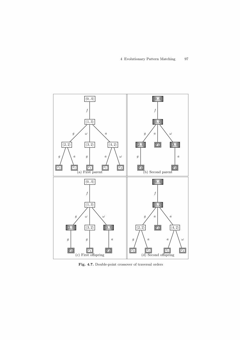
4 Evolutionary Pattern Matching 97
〈0, Λ〉
〈1, 3〉
f
〈2, 2〉
g
r3
g
r1
a
〈3, 2〉
ω
r1
g
〈4, 2〉
a
r1
a
r2
ω
(a) First parent
〈0, Λ〉
〈1, 2〉
f
〈2, 3〉
g
r3
g
r1
a
〈3, 3〉
ω
r2
a
(b) Second parent
〈0, Λ〉
〈1, 3〉
f
〈2, 3〉
g
r3
g
〈3, 2〉
ω
r1
g
〈3, 3〉
ω
r2
a
(c) First offspring
〈0, Λ〉
〈1, 2〉
f
〈2, 2〉
g
r3
g
r1
a
r1
a
〈4, 2〉
a
r1
a
r2
ω
(d) Second offspring
Fig. 4.7. Double-point crossover of traversal orders
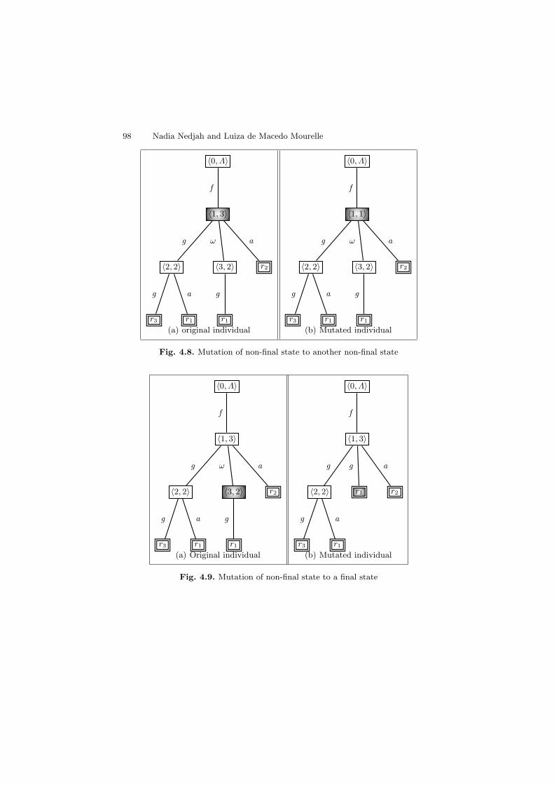
98 Nadia Nedjah and Luiza de Macedo Mourelle
〈0, Λ〉
〈1, 3〉
f
〈2, 2〉
g
r3
g
r1
a
〈3, 2〉
ω
r1
g
r2
a
(a) original individual
〈0, Λ〉
〈1, 1〉
f
〈2, 2〉
g
r3
g
r1
a
〈3, 2〉
ω
r1
g
r2
a
(b) Mutated individual
Fig. 4.8. Mutation of non-final state to another non-final state
〈0, Λ〉
〈1, 3〉
f
〈2, 2〉
g
r3
g
r1
a
〈3, 2〉
ω
r1
g
r2
a
(a) Original individual
〈0, Λ〉
〈1, 3〉
f
〈2, 2〉
g
r3
g
r1
a
r1
g
r2
a
(b) Mutated individual
Fig. 4.9. Mutation of non-final state to a final state

4 Evolutionary Pattern Matching 99
〈0, Λ〉
〈1, 3〉
f
〈2, 2〉
g
r3
g
r1
a
〈3, 2〉
ω
r1
g
r2
a
(a) Original individual
〈0, Λ〉
〈1, 3〉
f
〈2, 2〉
g
r3
g
r2
a
〈3, 2〉
ω
r1
g
r2
a
(b) Mutated individual
Fig. 4.10. Mutation of final state to another final state
4.5.4 Fitness function
When applied to a traversal order τ , the fitness function numerically measuresfour distinct aspects:
1. how sound is τ with regards to the given pattern set. In other terms, thefunction evaluates if the inspected positions for each pattern are valid forthat pattern. Given a pattern π, an inspected position may not be validfor two reasons: either it does not belong to the set of possible positionsfor π or its parent-position, which leads to it, was not inspected yet. Forinstance, let π = faωgωω, the set of valid position is Λ, 1, 2, 3, 3.1, 3.2.So if, for instance, positions 4 and/or 2.2 are present in the path in τthat declares a match for pattern π then τ is not a correct matchingautomaton for π. Moreover, if position 3.1 or 3.2 are inspected before orwithout position 3 being inspected, then τ is also not a correct automatonfor π. To measure this soundness factor, which we will denote by S , wesum up a non-soundness penalty ξS for each invalid position, and so wecan quantify the relation of soundness between two traversal orders τ1
and τ2. For pattern set Π, We say that τ1 is sounder than τ2 if and onlyif S (τ1,Π) < S (τ2,Π). The soundness factor for traversal order τ with

100 Nadia Nedjah and Luiza de Macedo Mourelle
respect to pattern set Π is defined as in (4.8). Note that for fully validtraversal orders, the soundness factor is zero. In the definition of (4.8) andfor the sake of functional programming, we use an extra parameter, whichwe call P and represent the set of positions present in the path visited bythe function. Initially, this parameter is the empty set.
S (τ,Π, P ) =
∑∀p∈P,pΠτ[0]
ξS , if #τ = 0
ξS +#τ∑i=1
S (τi,Π, P ∪ τi[0]), if τ [0] = x.p ∨ ∀y ∈ P, x = y
#τ∑i=1
S (τi,Π, P ∪ τi[0]), if τ [0] = x.p ∨ ∃y ∈ P, x = y
(4.8)2. how far does τ satisfy the termination property. In general, termination
is compromised when the traversal order inspects positions that are notindexes for the patterns in question. Considering the traversal order tree,this appears in the branches that are labelled by ω. So to quantify thetermination factor for τ , which we will denote by T (τ), we sum up anon-termination penalty ξT for each time ω appears as label in it. Thetermination factor for traversal order τ is defined as in (4.9). Note thattraversal orders that allow terminating rewriting sequences for all patternshave a termination factor zero. However, this is only possible for sequentialpatterns. Here, we deal with the more complicated case non-sequentialpatterns.
T (τ) =
0 if #τ = 0
ξT +#τ∑i=1
T (τi), if ∃j, 1 ≤ i ≤ #τ |τ [i] = ω
#tau∑i=1
T (τi), if ∀i, 1 ≤ i ≤ #τ |τ [i] = ω
(4.9)
3. how reduced is the code size of the automaton associated with τ . Asstate before, the code size of a matching automaton is proportional to thenumber of its states. So the code size for τ , which we will denote by C (τ),is simply the total state number in its traversal order. This defined as in(4.10).
C (τ) =
1 if #τ = 0
1 +#τ∑i=1
C (τi), otherwise(4.10)

4 Evolutionary Pattern Matching 101
4. how fast is pattern matching using τ . For a given pattern set, the timespent to declare a match of one the patterns is proportional to the numberof position visited. This can be roughly estimated by the length or numberof position in the longest path in the traversal order. However, a finermeasure of the matching time consists of computing the mean matchingtime for each pattern in the considered set, which is the average length ofall the paths that lead to the match of a given pattern, then computingthe mean time considering all the patterns in the set and using the socomputed mean matching time for each one of them. The matching timefor τ will be denoted by M (τ) and is defined in (4.11).
M (τ) =
1 if #τ = 0
1 + max#τi=1 M (τi), otherwise
(4.11)
The evolution of adaptive matching automata requires a multi-objectiveoptimisation. There are several approaches. Here, we use an aggregationselection-based method to solve multi-objective optimisation problems. It ag-gregates the multiple objectives linearly into a single objective function. Forthis purpose, it uses weights to compute a weighted sum of the objectivefunctions. The optimisation problem of adaptive matching automata has 4objectives, which are the minimisation of soundness (S ), termination (T ),code size (C ) and matching time (M ). The is transformed into a single ob-jective optimisation problem whose objective function is as (4.12):
min∀τ
F (τ,Π) = Ω1S (τ,Π) + Ω2T (τ) + Ω3C (τ) + Ω4M (τ) (4.12)
wherein Ωi are non-zero fractional numbers, usually called weights or impor-tance factors, such that we have Ω1 + Ω2 + Ω3 + Ω4 = 1.
Note the a weight value Ωi defines the importance of objective i. Therefore,to put more emphasis on valid adaptive matching automata, we give moreimportance to the soundness objective. The remaining objectives are of equalimportance.
4.6 Comparative Results
Optimisation using the weighted sum approach is extremely simple. It consistsof choosing a vector of weights and performing the optimisation process as asingle objective problem. As a single or limited number of solutions, hopefullyPareto-optimal [19], is expected from such process, it is necessary to performas many optimisation processes as the number of required solutions [16]. Inour experiments, we used the [0.4, 0.2, 0.2, 0.2] as weight vector.
The pattern matching automata for some known problems were used asbenchmarks to assess the improvement of the evolutionary matching automata

102 Nadia Nedjah and Luiza de Macedo Mourelle
with respect to the ones designed using known heuristics. These problems werefirst used by Christian [2] to evaluate his system HIPER. The Kbl benchmarkis the ordinary three-axiom group completion problem. The Comm benchmarkis the commutator theorem for groups. The Ring problem is to show that ifx2 = x is a ring then the ring is commutative. Finally, the Groupl problem isto derive a complete set of reductions for Highman’s single-law axiomatisationof groups using division.
For each of the benchmarks, we built the both matching automata, i.e. us-ing genetic programming and using known heuristics and obtained the numberof necessary states, matching time required. This should provide an idea aboutthe size of the automaton. Furthermore, we obtained the evaluation times ofa given subject term under our rewriting machine (for details see [14]) usingboth matching automata as well as the evaluation times of the same subjectterms under the system HIPER. The space and time requirements are givenin Table 4.1.
Table 4.1. Space and time requirements for miscellaneous benchmarks
Benchmark Number of states Number of states Time (s) Time (s)Classic Evolutionary Classic Evolutionary
Kbl 49 28 0.079 0.002Comm 153 89 1.229 0.211Ring 256 122 2.060 0.565Groupl 487 205 1.880 0.704
4.7 Summary
In this chapter, we presented a novel approach to generate adaptive matchingautomata for non-sequential pattern set using genetic programming. we firstdefined some notation and necessary terminologies. Then, we formulated theproblem of pattern matching and the impact that the traversal order of thepatterns has on the process efficiency, when the patterns are ambiguous. Wealso gave some heuristics that allow the engineering of a relatively good tra-versal order. In the main part of the chapter, we described the evolutionaryapproach that permits the discovery of traversal orders using genetic program-ming for a given pattern set. For this purpose, we presented how the encodingof traversal orders is done and consequently how the decoding of an evolvedtraversal order into the corresponding adaptive pattern-matcher. We also de-veloped the necessary genetic operators and showed how the fitness of evolvedtraversal orders is computed. We evaluated how sound is the obtained traver-sal. The optimisation was based on three main characteristics for matching

4 Evolutionary Pattern Matching 103
automata, which are termination, code size and required matching time. Fi-nally, we compared evolutionary adaptive matching automata, obtained forsome universal benchmarks, to their counterparts that were designed usingclassic heuristics.
References
1. A. Augustsson, A Compiler for Lazy ML, Proc. ACM Conference on Lisp andFunctional Programming, ACM, pp. 218-227, 1984. 82
2. J. Christian, Flatterms, Discrimination Nets and Fast Term Rewriting, Journalof Automated Reasoning, vol. 10, pp. 95-113, 1993. 82, 102
3. D. Cooper and N. Wogrin, Rule-Based Programming with OPS5, Morgan Kauf-mann, San Francisco, 1988. 82, 90
4. N. Dershowitz and J.P. Jouannaud, Rewrite Systems, Handbook of TheoreticalComputer Science, vol. 2, chap. 6, Elsevier Science Publishers, 1990. 82
5. A.J. Field and P.G. Harrison, Functional Programming, International ComputerScience Series, 1988. 82
6. J.A Goguen and T. Winkler, Introducing OBJ3, Technical report SRI-CSL-88-9,Computer Science Laboratory, SRI International, 1998.
7. A. Graf, Left-to-Right Tree Pattern-Matching, Proc. Conference on RewritingTechniques and Applications, Lecture Notes in Computer Science, vol. 488, pp.323-334, 1991. 82, 85, 86
8. C.M. Hoffman and M.J. O’Donnell, Pattern-Matching in Trees, Journal of ACM,vol. 29, n. 1, pp. 68-95, 1982. 82
9. P. Hudak and al., Report on the Programming Language Haskell: a Non-Strict,Purely Functional Language, Sigplan Notices, Section S, May 1992.
10. J.R. Koza, Genetic Programming. MIT Press, 1992. 9211. A. Laville, Comparison of Priority Rules in Pattern Matching and Term Rewrit-
ing, Journal of Symbolic Computation, n. 11, pp. 321-347, 1991. 83, 90, 9212. J.F. Miller, P. Thompson and T.C. Fogarty, Designing Electronics Circuits Us-
ing Evolutionary Algorithms. Arithmetic Circuits: A Case Study, In GeneticAlgorithms and Evolution Strategies in Engineering and Computer Science,Quagliarella et al. (eds.), Wiley Publisher, 1997. 94
13. N. Nedjah, C.D. Walter and S.E. Eldridge, Optimal Left-to-Right Pattern-Matching Automata, Proc. Conference on Algebraic and Logic Programming,Southampton, UK, Lecture Notes in Computer Science, Springer-Verlag, vol.1298, pp. 273-285, 1997. 82
14. N. Nedjah, C.D. Walter and S.E. Eldridge, Efficient Automata-Driven Pattern-Matching for Equational programs, Software-Practice and Experience, John Wi-ley Eds., vol. 29, n. 9, pp. 793-813, 1999. 86, 87, 102
15. N. Nedjah and L.M. Mourelle, Implementation of Term Rewriting-Based Pro-gramming Languages, Hauppauge, NY, ISBN 1594-5439-09, 2005. 82, 83
16. N. Nedjah and L.M. Mourelle (Eds.), Real-World Multi-Objective Systems En-gineering, Nova Science Publishers, Hauppauge, NY, ISBN 1590-3364-53, 2003. 101
17. N. Nedjah and L.M. Mourelle, More Efficient Left-to-Right Matching for Over-lapping Patterns, vol. 3, n. 2-4, pp. 230–247, 2005. 88
18. M.J. O’Donnell, Equational Logic as Programming Language, MIT Press, 1985. 82

104 Nadia Nedjah and Luiza de Macedo Mourelle
19. V. Pareto, Cours d’economie politique, volume I and II, F. Rouge, Lausanne,1896. 101
20. R.C. Sekar, R. Ramesh and I.V. Ramakrishnan, Adaptive Pattern-Matching,SIAM Journal, vol. 24, n. 5, pp. 1207-1234, 1995. 82, 83
21. D.A. Turner, Miranda: a Non Strict Functional Language with PolymorphicTypes, Proc. Conference on Lisp and Functional Languages, ACM, pp. 1-16,1985.
22. P. Wadler, Efficient Compilation of Pattern-Matching, In “The Implementa-tion of Functional Programming Languages”, S. L. Peyton-Jones, Prentice-HallInternational, pp. 78-103, 1987. 82

5
Genetic Programming in Data Modelling
Halina Kwasnicka1 and Ewa Szpunar-Huk2
1 Institute of Applied Informatics, Wroclaw University of Technology, Wyb.Wyspianskiego 27, 50-370 Wroclaw, Poland [email protected]
2 Institute of Applied Informatics, Wroclaw University of Technology, Wyb.Wyspianskiego 27, 50-370 Wroclaw, Poland [email protected]
The chapter presents some abilities of Genetic Programming (GP), one of thebranches of Evolutionary Computation (EC), which becomes very popular indifferent areas, such as Data Modelling (DM). In this chapter attention isfocused on using GP to make data collected in large databases more usefuland understandable. Here we concentrate on such problems as mathematicalmodelling, classification, prediction and modelling of time series. Successivesections are dedicated to solving the above mentioned problems using the GPparadigm. Sections devoted to individual problems share a similar structure:their first parts characterise the specificity of a given problem with respectto applying GP to the task under consideration, the second parts describeexamples of using GP in such a problem and the final parts contain generalinformation connected with the issue being discussed in the first two parts.The chapter begins with a short introduction to Data Modelling and GeneticProgramming. The last section recapitulates the chapter.
5.1 Introduction
Evolutionary Computation paradigm becomes very popular. A number ofapproaches that exploit the biological evolution ability to adaptation arise.Between them we can distinguish Genetic Algorithms, Evolutionary Strate-gies and Evolutionary Programming. Genetic Programming (GP) proposedby Koza use the same idea as Genetic Algorithm (GA) and it is perceived asa part of GA. The main difference is that GP use different coding of poten-tial solutions, what forces different genetic operators such as crossover andmutation. The main idea of Evolutionary Computation is to imitate naturalselection, that is the mechanism that relates chromosomes with the efficiencyof the entity they represent, thus allowing those efficient organisms, which are
H. Kwasnicka and E. Szpunar-Huk: Genetic Programming in Data Modelling, Studies in Com-putational Intelligence (SCI) 13, 105–130 (2006)www.springerlink.com c© Springer-Verlag Berlin Heidelberg 2006

106 Halina Kwasnicka and Ewa Szpunar-Huk
well-adapted to the environment, to reproduce more often than those whichare not.
Genetic Programming is strongly developed in different places – univer-sities, laboratories etc. The web http://www.genetic-programming.org/ is areach source of knowledge dedicated to GP. The readers can find there use-ful both theoretical and practical information. Genetic Programming is verypopular everywhere, where the algorithm to solve a considered problem is notknown, because GP starts from a high-level statement of ”what needs to bedone”. A computer program solving the problem is evolved, what means – itis developed automatically.
The chapter concerns the problem connected with making a great amountof data, collected in different places (firms, consortia, etc.), useful. Discover-ing knowledge from possessed data and making it useful is very importantespecially for managers.
The chapter, beside Introduction and Summary, consists of the three mainsections. Section 5.2 gives introduction and the example of using Genetic Pro-gramming for mathematical modelling task. Section 5.3 details the GeneticProgramming used for classification task, where of course, we can use somerules induction and decision trees generation algorithms, but as we can see, insame cases Genetic Programming can reveal some advantages. Other impor-tant problems are connected with prediction and time series modelling. GPcan also be used for these tasks. The third main section (Section 5.4) presentshow GP can be used for such problems. Some conclusions are placed in thelast section – Summary (Section 5.5).
5.2 Genetic Programming in Mathematical Modelling
Mathematical modelling can be regarded as a search for equations that pro-vide a good fit to numerical data. It is used in variety of problems like scientificlaw discovery or prediction tasks in fields where the theory does not give def-inite answers about the outcome of experiments. The search process howeverusing traditional methods, for example polynomial regression, is often diffi-cult, because in these methods a specific model form must be assumed, whatdemands strong theoretical knowledge. Usually in case of regression only thecomplexity of this model can be varied so the search task is often limited tofinding a set of coefficients. GP allows searching for a good model in a different,more ”intelligent” way, and can be used to solve highly complex, non-linear,probably chaotic or currently not fully or properly understood problems [1].
Induction of mathematical expressions on data using GP is introducedby Koza and is called symbolic regression [2], to emphasise the fact thatthe object of search is a symbolic description of a model, not just a set ofcoefficients in a prespecified model. Koza showed that GP could perform wellin function identification tasks, because it searches the space of all possiblemodels for both a good model form and the appropriate numeric coefficients

5 Genetic Programming in Data Modelling 107
for the model. The search space is constrained only by the available modelpieces (variables, functions, binary operators, syntax rules). Furthermore, GPis not obligated to include all input variables in the equation, so it can performa kind of dimensionality reduction.
5.2.1 Adaptation of GP to Mathematical Modelling
Genetic programming can be successfully used to find a mathematical datamodel because it can find the shape of the equation as well as the compo-sition of primitive functions, input variables and values of coefficients at thesame time, without any additional information except the performance of theanalysed expression on the data. But the key issue to make GP algorithmwork is a proper representation of a problem, because GP algorithms directlymanipulate the coded representation of equation, which can severely limit thespace of possible models. An especially convenient way to create and manipu-late the compositions of functions and terminals are the symbolic expressions(S-expressions) of the LISP programming language. In such a language themathematical notation is not written in standard way, but in prefix notation.It allows building expression trees out of these strings, that can be easilyevaluated then. Some examples of expressions written in algebraic and prefixnotation with corresponding trees are shown in Fig. 5.1.
Fig. 5.1. An examplary tree in GP and the coded expression
In the Genetic Programming paradigm, the individuals in the popula-tion are compositions of functions and terminals appropriate to the partic-ular problem’s domain. Functions and terminals are adequately nodes andleaves of the trees being evolved by the GP. Therefore, before running GPto search for an equation, it is necessary to define operators dedicated to

108 Halina Kwasnicka and Ewa Szpunar-Huk
the considered task. For the mathematical modelling problem the four binaryarithmetic functions (+, -, *, /) are usually used, but other specific functions(e.g., trigonometric functions, sqrt, abs) can also be useful. The terminals orleaves are either variables or coefficients. Variables correspond to the databeing analysed, while coefficients are defined by numerical ranges.
Using arithmetic functions as operators in GP has some drawbacks. Oneof them is that the closure property of GP requires, that each of the basefunctions is able to accept, as its arguments, any value that might possibly bereturned by any base function and any value that may possibly be assumed byany terminal. This condition is not satisfied by e.g., division operator. Thatis why a protected division function div(a, b) is usually defined which returns1 in two cases: when a = b and when b = 0. Otherwise it returns a resultof division a/b. Similar protections must be established for many other func-tions as e.g., log(a) or sqrt(a). The problem with closure property is entirelyeliminated in Strongly Type Genetic Programming (STGP) [4], in which itis assumed that each function specifies precisely the data types of its argu-ments and its returned values, but on the other hand, additional modificationsof the searching process are required, like creating more individuals in eachgeneration in order to better explore the search space.
During the evaluation of GP solution some numerical problems may alsoeasily occur, like underflows or overflows caused by extremely small or highvalues or major precision loss, e.g., determining a trigonometric function suchas sin(a) for some value a much larger than 2Π [5]. It is also assumed thatthe creation of floating-point constants is necessary to do symbolic regressionand it seems to be a weak point, because coefficient must be assembled fromrandom values, so destination functions containing constants are usually muchmore demanding to GP than others. Designing GP algorithm to mathematicalmodelling it is necessary to consider most of these problems.
5.2.2 An educational Example – the Hybrid of GeneticProgramming and Genetic Algorithm
In this section we present a detailed description of a simple GP algorithm tomathematical model induction. The work was done as a part of wider study ofSzpunar-Huk, described in [24]. The goal of the designed algorithm is to finda function y = f(x1, ..., xn), which reflects potentially existing relationshipbetween input and output values. As the input data we have a sample setS =x1, ..., xn, y, where x1, ..., xn are independent input values and y is anoutput value (assumed function of xi). Values x1, ..., xn and y are continuousnumbers converted to floating point numbers with a specified for an individualexperiment precision. The algorithm is tested to examine its ability to dosymbolic regression on sample sets of different size and level of noise, generatedusing predefined mathematical functions, and for different evolution controlparameters (e.g., population size, probabilities of crossover and mutation).

5 Genetic Programming in Data Modelling 109
During experiments generations’ numbers with standard deviations needed tofind solutions and obtained errors were analysed.
Firstly it is important to define terminals and functions sets used for ap-proximating the test functions. Let us assume:
• The terminal set T =x1, ..., xn, R – the set of possible values of leavesof trees being evolved contains input variables’ labels and continuous con-stants between 1.0 and 100.0.
• The set of available base functions F =+,−, ∗, / include just addition(+), subtraction (–), multiplication (∗) and division operator (/).
It is important to notice, that in this case the division operator is not pro-tected, so the closure property of GP is not satisfied. This problem is solvedby a proper definition of the fitness function. All the base functions have twoarguments what significantly simplifies crossover operation.
A fitness function measures how well each individual (expression) in thepopulation performs the considered problem (task). In described experimentstwo fitness functions were used. The first one was the sum of errors made byan individual on a sample set and could be written as:
F =N∑
i=1
|ex(xi) − yi| (5.1)
where N is a number of samples in the set S, ex(xi) is a value returned byan expression ex (encoded expression by the considered individual) for the ith
sample, yi is a value of output y for ith sample.The second function was the average percentage errors made by an indi-
vidual on a sample set and could be written as:
F =1N
∗N∑
i=1
100 ∗ |ex(xi) − yi|ex(xi)
(5.2)
where as before, N is a number of samples in the set S, ex(xi) is a valuereturned by an expression ex for the ith sample, yi is a value of output y forith sample.
For both functions, the closer the sums are to zero, the better the ex-pressions (solutions) are. Additionally, when during evaluation of a given ex-pression on any sample from a sample set, division by zero occurs, the fitnessfunction for the individual is set to ”undefined”. It is also worth mention, thatin case of the first function, when the values returned by the sample are closeto zero, it is difficult to distinguish between good and bad individuals, whatcan significantly affect GP performance, but due to the specific of chosen datait was not important in the described experiments.
In the selection phase couples of individuals for crossover are chosen. As aselection method here is proposed the method based on elite selection. Firstly

110 Halina Kwasnicka and Ewa Szpunar-Huk
all individuals are ranking according to their fitness (expressions with ”unde-fined” value are placed on the end of the list). Secondly a number of the bestdifferent individuals (the exact number is set by an appropriate parameter –usually it is about 10% of population size) are taken to the next generationwithout any changes. A reason for this is that in GP during crossover phaseexpressions cannot evolve well because they are frequently destroyed and itis easy to loose the best ones, what can result in poor performance. Selectedindividuals must be also different to avoid premature convergence of the algo-rithm. The remaining couples for the crossover phase are generated as follows:the first individual is the next individual from the ranking list (starting fromthe best one), the second one is randomly chosen from the whole population,not excluding expressions with ”undefined” value.
After selection a number of couples (according to a given probability pa-rameter) are copied to the next generation unchanged, the rest individualsundergo the crossover – a random point is chosen in each individual and thesenodes (along with their entire sub-trees) are swapped with each other, cre-ating two entirely new individuals, which are placed in the new generation.In the classical GP, each tree could be of potentially any size or shape, butfrom the implementation point of view, every new tree can not be biggerthen the predefined maximum depth, so if too deep tree is generated duringcrossover operation, it is being cut to the maximum allowed size. Here, inthe recombination operation another parameter is also introduced. The para-meter specifies probability of choosing a leaf as a place of crossing, becausechoosing a random point can result in fast shortening of all individuals in thepopulation.
Mutation is an additional included genetic operator. During mutation op-eration nodes or leafs are randomly changed with a very little probability,but over a constraint, that the type of node remains unchanged: a terminalis replaced by an another terminal and a function by an another function.It is difficult to estimate the real size of a population mutation since, duringreproduction phase – when maximum depth of tree is established – trees areoften cut, what also can be viewed as a kind of mutation.
An initial population is randomly generated, but creating a tree with max-imum depth is more likely to come than creating a tree with only one or justfew nodes.
Experiments
To validate described method, some numerical experiments were conducted.In this case some sample sets were generated according to a given functionf , the algorithm was looking for this function, but a sample could containmore variables than it was used by the given function. The algorithm turnedout to be a good tool to exactly discover plenty of functions. Table 5.1 showssome examples of mathematical expressions, the algorithm managed to findin generated data, and the average number of needed generations of the al-gorithm. During this experiments the number of input variables’ labels in the

5 Genetic Programming in Data Modelling 111
Table 5.1. Sample of test functions and number of generations needed to find thatfunction by the algorithm
Function Number of generations
y = x1x1x1 3y = x3 + x2x1 − x4 8y = x1/(x2 + x3) 16y = x1 + x1x1 − x2/x3 22y = x1 + x2 + x3 + x4 + x5 + x8 + x7 + x8 31y = x1 + x2/x3 − x3/x1 45y = x3x2/(x5 + x4) − x4 103y = x1 + x2/x3 + x3x4 − (x3 + x3)/x2 135y = 10x1 + 5x2 137y = x1 + x2 + x3x3 − x1x1x1/(x2x2) 207y = x1 + x2 + x3 + x4 + x5 + x8 + x7 + x8 + x2x3x4 375y = x1x1x1 + x2x2x2 + x3x3x3 + x4x4x4 579
sample set and the number of different input variables in the equation whereequal. In a number of experiments the vector of input variables xi containsa variables that are not taken into account during output calculation, theyare additional variables. It means that our algorithm looks for the functiony = f(x1, ..., x10) but the proper dependency is y = f(x1, x2) – only two inputvariables influence the output variable. In such cases the algorithm could alsofind the relationship, but in longer time. A number of redundant variables wedenote by Nadd, Tsolution means an average number of generations for findingsolution, but δadd – a standard deviation of Tsolution. Exemplary results areshown in table 5.2. It is important to mention that the algorithm requires
Table 5.2. The result given by GP+GA for different number of additional variables
Nadd Tsolution δadd
0 8.71 1.91 17.4 5.912 19.7 5.083 20.7 6.754 29.7 12.45 37.4 14.26 42.1 30.6
various control parameters to proper working. Some of them are mentionedabove. The most important of them with their presumed values are listed be-low. They are suggested values, often used in the experiments, but in sometasks their values must be carefully tuned.A list of control parameters of GP used in the experiments:

112 Halina Kwasnicka and Ewa Szpunar-Huk
• Population size: 300-400• Maximum depth of the tree: 6-8• Percent of individuals moved unchanged to the next generation: 10-30%• Crossover probability: 0.85• Probability of choosing leaf as a crossing point: 0..1• Mutation probability: 0.01.• Number of samples: 100-1000
Tuning of the Algorithm
The algorithm in such a form is able to find hidden model in a sample seteven with noisy data – the output was generated not exactly from a givenfunction, but outputs were in 5%, 10% or even more noisy. Difficulties howeverappeared when a tested function included coefficients, especially with realvalued coefficients. It is not possible to find relationships, even if it seems tobe easy (e.g., y = 15x1 + 4x2 − 23.4x3/x2). Enlarging the initial populationsize from 500 to 5000 individuals can partially solve this problem, but forplenty of functions it is not sufficient.
To make the algorithm more effective an additional algorithm based onthe classic Genetic Algorithm is included. The aim of this algorithm is tofind, for a given set of best individuals, after a given number of generations inGP, as good coefficients as possible. That is why the algorithm is cold TuningAlgorithm (TA).
The tuning algorithm works as follows: for the given individual taken fromthe GP algorithm a number of coefficients is established. This number definesa length of individuals in the TA, where an individual is a sequence of num-bers from the given range and with a given precision. An initial populationof the TA contains sequences generated on an expression taken from the GPalgorithm and random sequences – one hundred individuals altogether. Gen-erated in such a way population is evolved in the standard way: individualsare selected, crossed over and mutated. The fitness function and the selectionoperation are the same as in the GP algorithm, but the crossover operation ismuch simpler: for a given couple of individuals a random point in constantssequence is chosen (the same for both individuals) and a part of one indi-vidual is swapped with a part of the second one, what is shown in Fig. 5.2.Mutation however is much more important here than in GP algorithm. Itsaim is to make it possible to tune the coefficients. A special kind of mutationis proposed. Each real number is a set of Arabic numeral, e.g., 13.86 consistsof digits 1, 3, 8 and 6. The probabilities of mutation of particular digits aredifferent – the lowest is for the digit placed on the left (the most meaningful)and systematically is increased for the next digits (going to the right). Thescheme of the whole algorithm (GP connected with TA) is shown in Fig. 5.3.The tuning process is performed every N generations of GP for S different,best individuals from an actual generation of the GP. Incorporating of a GAallows approximation of relationships previously impossible to find. For exam-

5 Genetic Programming in Data Modelling 113
Fig. 5.2. An example of crossover in TA
ple, when the dataset was generated using equation 5.3, the GP has problemwith finding the exact coefficients.
y = 11.3/x2 + 10x3x3 − 5.2x2/(x3 + x5) + 33.8x3x3x3x5x6x6++20(x4 + x2)/x5 + 8x5x5x5 + 12(x3 + x5)/x2 + x3x3x3
(5.3)
Using the tuning algorithm worked every 40 generations of the GP on 15best individuals after 100 generation of GP, the average percentage error ofthe best individual on dataset was equal to 1.2% while without tuning only9.25%.
Input: X, YOutput: Expression y’≈ f(X)1. Create an initial GP population and set GN (number of generations) to 02. Evaluate the fitness of the population members3. While termination criteria not met do4. If GNmodN = 0 perform tuning5. Take S individuals for tuning6. For each of S chosen individuals do7. Create an initial GA population8. Evaluate the fitness of the population members9. While termination criteria not met do10. Probabilistically apply crossover operator11. Probabilistically apply mutation operator12. Go to step 813. Probabilistically apply crossover operator14. Probabilistically apply mutation operator15. Increase GN16. Go to step 217. End.
Fig. 5.3. The scheme of the GP in conjunction with GA used as TA algorithms
5.2.3 General Remarks
In the presented example abilities of GP algorithm to discover mathemati-cal model on artificially generated data where shown, but approximation afunction using a given finite sample set of values of independent variables and

114 Halina Kwasnicka and Ewa Szpunar-Huk
associated values of dependent variables is a very important practical prob-lem. In practice, the observed data may be noisy and there may be no knownway to express the relationships involved in a precise way. That is why GP iswidely used to solve the problem of discovering empirical relationships fromreal observed data. To show, how wide variety of domains GP is successfullyapplied some of experiments with GP on real data are mentioned below.
Koza [3] showed, how the Genetic Programming paradigm can be usedto create an econometric model by rediscovering the well-known non-lineareconometric ”exchange equation” M = PQ/V , which relates the money sup-ply M , price level P , gross national product Q, and the velocity of moneyV in economy. He also showed how Kepler’s Third Law can be rediscovered.Sugimoto, Kikuchi and Tomita were able, by applying some improvementsto GP, to predict an equation from time course data without any knowledgeconcerning the equation. They predicted biochemical reactions and the rela-tive square error of predicted and given time-course data were decreased, dueto GP, from 25.4% to 0.744% [6]. Langdon and Barrett have used GeneticProgramming (GP) to automatically create interpretable predictive modelsof a small number of very complex biological interactions, which are of greatinterest to medicinal and computational chemists, who search for new drugtreatments. Particularly, they have found a simple predictive mathematicalmodel of human oral bioavailability [7]. Makarov and Metiu use GP to theanalytic solutions of the time-independent Schrodinger equation. They testedtheir method for a one-dimensional enharmonic well, a double well, and atwo-dimensional enharmonic oscillator [8]. Diplock, Openshaw i Turton usedGP as a tool for creating new models of complex geographical system. Theyrun parallel GP algorithm on Cray T3D 512 supercomputer to create newtypes of well performing mathematical model [9].
It is important to notice that in scientific discovery however, obtainingsome adequate fit to data is not enough. To fully incorporate some results inthe body of scientific work, it is necessary that some form of understandingabout the expressions that are induced is achieved. The expressions thus needsome further justification before they can be used as models of the phenom-enon under study. The resulting equations can then be tested with statisticalmethods to examine their ability to predict the phenomenon on unseen data.
5.3 Decision Models for Classification Tasks
Classification task is the one of fundamental and the most studied tasks inthe area of data mining. Given a set of predetermined, disjoint target classesC1, C2, ..., Cn, a set of input attributes A1, A2, ..., Am, and a set of trainingdata S with each instance associated with a unique target class label, theobjective of this task is to find mutual properties among a set of objects indata set which can be used to determine the target category for new unseendata given its input attributes’ values. In the other words, this process finds

5 Genetic Programming in Data Modelling 115
a kind of decision models – a set of classification rules (or procedures insome cases). Classification rules are commonly expressed in the form of IF-THEN rules, where the IF part of a rule contains a logical combination ofconditions on the attributes and the THEN part points to a class label. Thepopular decision model is also a decision tree, in which the leaves are theclass labels while the internal nodes contain attribute-based tests and theyhave one branch emanating for each possible outcome of the test.
Most rules induction (e.g., CN2 ) and decision trees generation algorithms(e.g., CART and C4.5 ) perform local, greedy search to generate classificationrules, that are relatively accurate and understandable, but often more complexthan necessary. There are several properties of GP, which make them moreconvenient for application in data mining tasks comparing to other techniques.The reason is that the local, greedy search selects only one attribute at a time,and therefore, the feature space is approximated by a set of hypercubes. Inreal-world applications, the feature space is often very complex and a large setof such hypercubes might be needed to approximate the class boundaries. GPalgorithms perform global search. That is why it copes well with attributesinteraction problem, by manipulating and applying genetic operators on thefunctions. Additionally some data mining algorithms work only with qualita-tive attributes, so numerical values must be divided into categories. GP candeal with any combination of attribute types. Moreover, GP algorithms haveability to work on large and ”‘noisy” datasets. They have the high degree ofautonomy that makes it possible to discover of knowledge previously unknownby the user.
5.3.1 Adaptation of GP to Clasification Task
Classification task is similar to the regression, and regression could also beused to solve some classification problems but generally, building decisionmodels emphasis on discovering high-level, comprehensible classification rulesrather than just producing a numeral value by a GP tree. Application of GPin this field is similar, but due to some differences, causes additional problems.
Problems with Closure Property
The main difference between using GP in classification and regression tasksis that in classification the target class (the goal attribute) is nominal whilein regression – continuos one. When data set contains mixture of real-valuedand nominal attribute values, different attributes are associated with differentfunctions, so the closure property is usually not satisfied by the standard GPalgorithm and the closure problem is much more complicated. One idea tosolve the problem is to use logical operators for all inner nodes, while leaveshave only boolean values or are represented as functions that return Booleanvalues. Other approaches to go around the closure requirements are STGP,mentioned in section 5.2.1 [4, 10] (sometimes called constrained-syntax GP),

116 Halina Kwasnicka and Ewa Szpunar-Huk
and its variant called Grammar-Based Genetic Programming (GBGP) [10].The key idea of STGP is such, that for each function f from a set of func-tions, the user specifies which terminals/functions can be used as a childrennode containing function f . In GBGP syntactic and semantic constraints arespecified by a grammar [10, 14], so the important preparation step for theGP is to identify a suitable target language, in which to evolve programs. Itshould be underlined, that the success of evolution is dependent upon the useof a language, that can adequately represent a solution to the problem beingsolved.
Michigan – Pittsburgh Approaches
The next step designing a GP for discovering decision model, after choosinga proper language, is to choose individual representation. There are two mainapproaches to use GP algorithms to classification rule discovery, based on howrules are encoded in the population of individuals: the Michigan [11] and thePittsburgh approach [11]. In the Michigan approach each individual encodes asingle classification rule, whereas in the Pittsburgh approach each individualencodes a set of classification rules. The choice of individual representationdetermines the run of GP algorithm. The Michigan is best suitable for binaryclassification problem, where there are only two classes to distinguish and oneindividual is entire solution for the problem. The problem gets more compli-cated when there are more then two classes in the classification task but thisapproach is also used in such problems. The most common solution for thisin the literature is to run the GP k times, where k is the number of classes[12]. In the ith (i = 1, ..., k) run, the GP discovers rules for the ith class. WhenGP is searching for rules for a given class, all other classes are merged intoa large class. In the Pittsburgh approach GP can work with a population ofindividuals where each individual corresponds to a rules set, constituting acomplete solution for the classification problem, i.e. entire decision tree [11].
Fitness Function Defining
Discovering useful decision models desiring goal is to obtain rules, which areboth accurate and comprehensible. The fitness function evaluates the qual-ity of each rule. Majority of fitness functions used in GP grew out of basicconcepts on classification rule evaluation. They usually use TP , FP , TN andFN factors which, for a given rule of the form IF condition (A) THENconsequent (B), denote respectively:
• TP (True Positives) – a number of examples satisfying both A and B,• FP (False Positives) – a number of examples not satisfying A but satisfying
B,• FN (False Negatives) – a number of examples not satisfying both A and
B,• TN (True Negativess) – a number of examples satisfying A but not B.

5 Genetic Programming in Data Modelling 117
To rely on these factors several formulas used in fitness function have beendescribed in the literature [14], i.e.,
• confidence: (co = TP/(TP + FP )• consistency (cs = TP/(TP + TN)• sensitivity (Se = TP/(TP + FN))• specificity (Sp = TN/(TN + FP )
A fitness function usually contains combination of such formulas, e.g., fitness =Se ∗ Sp [19]. Selection of factors appearing in the fitness function clearly de-pends on the type of the task and desired characteristics of the discoveredsolution. In the Pittsburgh approach, where one individual is the entire solu-tion, the most popular method to evaluate solutions is accuracy rate, whichis simply the ratio of the number of correctly classified test examples over thetotal number of test examples.
Adjusting properly the fitness function can also addressed the problemof the comprehensibility of the discovered rules. Beside the accuracy of theclassification rules on the data set, the function can also take into account asize of the tree, penalising the trees with the high number of nodes. Noda etal. introduced additionally a rule ”interestingness” term in the fitness functionin order to discover interesting rules [15].
5.3.2 An Example of Classification Rules Discovering using GP
This section contains a description of a successful application of GP to a clas-sification task. As an example we propose research of Ross, Fueten and Yashir[16]. They used GP to solve the problem of identification of microscopic-sizedminerals involved in rocks. Mineral identification is a task, that usually donemanually by an expert, who uses various visual cues like colour, texture andthe interaction of the crystal lattice with different directions of polarised light.It is worth to stress, that proper identification by a human is time-consumingand requires years of experience.
GP algorithm is used by Ross et al. to develop a decision tree from data-base, which contain 35 colour and texture parameters of mineral specimens’feature. This database was used also to manual mineral identification. Theseparameters were obtained by multiple-stage process of mineral sample imagesanalysis. Their approach is a Michigan approach, so the algorithm producesone decision tree specialised for identifying a specific mineral. Such a tree,given a sample of data for a grain, can determine, if the grain corresponds tothe mineral, the tree is engineered to recognise. Thus decision model consistsof several decision trees, one for each mineral species.
5.3.3 Used Algorithm
To represent solution two languages were proposed, so it is a Grammar-Based Genetic Programming algorithm. The Backus-Naur grammar for thelanguages is as below:

118 Halina Kwasnicka and Ewa Szpunar-Huk
L1: Bool ::=if Param < Param then Bool|Param<Param |True|False
Param ::=p1|p2|...|p35|<ephemeral const>L2: Bool ::=if Bool then Bool else Bool|Bool and Bool
|Bool or Bool|not Bool|E BoolRel E|True|False
BoolRel ::=<|<=|>|>=|=E ::=E Op E|max(E1,E2)|min(E1,E2)|ParamOp :=+|-|/|*Param ::=p1|p2|...|p35<ephemeral const>
The first language L1 consists only of If-Then statements, a relational op-erator ”<” over the 34 parameter values and the logical constants True andFalse, while L2 is more complex and introduces mathematical expressionsover parameter values. Ephemeral constants in L2 are floating-point numbersbetween 0.0 and 1.0 and relational ”<” statement work with a degree of errorwithin 10% of the left-hand parameter. For example, in the expression ”a=b”,if b is within 10% of value of a, the expression returns True. Additionally, forL2 language it was necessary to modify division operator ”/” to satisfy clo-sure property. Thus this operator returns ”0”, if division by zero appears. Theindividual coded in both languages return True, if the analysed grain para-meters conform to the particular mineral, that the tree is designed to identify,and False otherwise.
The data set for evolution and experiments contained 11 mineral speciesand varied number of examples of each mineral: quartz (575), K-spar (369),plag (358), biotite (74), muscovite (36), hornblende (86), CPX (81), olivine(685), garnet (311), calcite (520) and opaque (189). The data set was preparedwith participation of geologist. For a given mineral selected for one evolutionprocess, training and testing data are chosen from the entire data set. Thetraining data set consists of a random selection of K samples of mineral beingidentified and a random selection of K samples for each of the other minerals,so the total number of training examples is N*K, where N is the number ofmineral species.
The fitness function used during evolution for a distinguished mineral Mis the following:
Fitness =12K
(Hits
K+
Miss
(N − 1)
)(5.4)
where Hits is the hits correct number – the number of correctly identifiedgrains of mineral M and Miss is the misses correct number – the number ofgrains correctly identified as not being mineral M, K – a number of samplesof M in the training set.
Experiments were carried out for two kinds of training sets. The first onecontained 34 positive examples and 340 negative examples per run, in the sec-ond one the number of positives examples were doubled to 70. For experimentsof the second type four of the eleven minerals (biotite, muscovite, hornblende

5 Genetic Programming in Data Modelling 119
and CPX) had to be excluded, because they provided insufficient numbersof positive examples in the grain database to permit accurate training andtesting. The testing set was the rest of the database not used for training.The testing formula was similar to the fitness formula:
Performance =12
(Hits
P+
Miss
Q
)100% (5.5)
where P is the total number of grains for mineral M in the testing set, andQ is the total number of other grains. Table 5.3 shows obtained results of GP
Table 5.3. Obtained result in Minerals classification [16]
L1 L2 NNK 34 70 34 70 74Mineral Test Train Test Train Test Train Test Train Test
Quartz Best: 90.2 94.6 92.2 93.8 93.5 97.5 97.8 96.1 96.5Av.: 84.7 90.9 85.7 88.9 88.3 93.7 90.1 92.5
K-spar Best: 94.2 97.8 93.9 96.0 93.8 99.0 93.4 96.9 88.6Av.: 89.7 95.9 91.0 93.5 90.7 97.8 90.8 93.0
Plag Best: 86.2 91.8 84.7 93.8 83.3 95.7 95.4 94.3 89.1Av.: 75.8 88.0 78.9 88.9 78.6 91.8 80.2 93.0
Biotite Best: 98.1 98.1 – – 96.6 99.4 – – 97.3Av.: 93.7 96.4 92.7 98.0
Muscovite Best: 98.3 6.6 – – 97.6 99.9 – – –Av.: 74.8 94.1 78.0 98.0
Homblende Best: 91.4 97.7 – – 92.8 98.5 – – 95.4Av.: 86,8 94.7 86.1 95.8
CPX Best: 90.3 96.5 – – 93.8 98.5 – – 97.5Av.: 81.0 88.1 84.9 92.8
Olivine Best: 90.0 94.4 89.9 93.8 91.4 96.6 93.2 98.1 92.8Av.: 83.0 88.6 85.6 90.0 84.4 92.6 89.4 95.1
Garnet Best: 98.2 99.7 99.6 99.6 97.8 100 99.4 99.8 97.4Av.: 96.0 98.3 97.6 98.1 95.8 98.9 97.1 98.6
Calcite Best: 92.1 97.4 91.8 95.2 92.8 99.0 95.1 98.2 96.0Av.: 84.4 93.6 88.5 93.0 86.2 98.3 91.2 95.9
Opaque Best: 97.7 99.9 97.7 99.9 98.3 100 98.1 100 95.2Av.: 93.6 98.9 96.6 99.4 95.2 99.3 96.5 99.7
runs and, for comparison, the results of testing performance for the same databy neural network (NN) proposed by Thompson et al. [17], trained to identifyall the minerals with one single network.
Experiments showed that GP was successfully applied to mineral classifi-cation task. The overall performance of the best obtained mineral identifiersranged from 86% to 98%. The authors noticed that the language L2, whichis more complex than L1, did not lend any great advantages to the quality of

120 Halina Kwasnicka and Ewa Szpunar-Huk
solutions but is computationally more expensive due to arithmetic operators.Solutions obtained using more positive grain examples was normally advanta-geous to the average quality of solutions, but in most of the cases for L1, thesolutions for K = 70 were not significantly better than those for K = 34 andoften suffered from over-training effects. The GP performance is comparableto that obtained with a performance of NN, but obtained models are not a”black-box” and are quite short and possible to understand by a human.
5.3.4 General Remarks
Many companies collect vast amounts of data, however they fail to extractnecessary information to support managerial decision-making. That is whyclassification is an important problem extensively studied in several researchareas. Classification systems can find in databases meaningful relationshipsuseful for supporting a decision making process or automatic identifying ob-jects in medicine, astronomy, biology etc., that might take years to find withconventional techniques.
GP was used for deriving classification models from data especially in med-ical and financial domains. As an example the Gray’s and Maxwell work onusing GP to classify tumours based on H Nuclear Magnetic Resonance spectracan be mentioned [12]. They proposed a new constrained-syntax Genetic Pro-gramming and reported, that the algorithm can classify such data well. Otherexample could be one of the newest researches made by Bojarczuk et. al., whoproposed new constrained-syntax Genetic Programming algorithm for discov-ering classification rules [12]. They tested their algorithm on five medical datasets such as: Chest pain, Ljubljana breast cancer, Dermatology, Wisconsinbreast cancer and Pediatric Adrenocortical Tumor and obtained good resultswith respect to predictive accuracy and rule comprehensibility, by comparisonwith C4.5 algorithm [18]. Another interesting work was presented by Bentley,who used GP to evolve fuzzy logic rules capable of detecting suspicious homeinsurance claims. He showed that GP is able to attain good accuracy andintelligibility levels for real, home insurance data, capable of classifying homeinsurance claims into ”suspicious” and ”non-suspicious” classes [19].
Usually databases considered in data mining (DM) tend to have gigabytesand terabytes of data. The evaluation of individual against the database isthe most time consuming operation of the GP algorithm. But thanks to vari-ety of possible modifications and parallel approaches to Genetic Algorithms,scalability of these algorithms can be achieved.
5.4 GP for Prediction Task and Time Series Odelling
The amount of data stored in different databases continues to grow fast.This large amount of stored data potentially contains valuable, hidden knowl-edge. This knowledge could be probably used to improve the decision-making

5 Genetic Programming in Data Modelling 121
process. For instance, data about previous sales of a company may containinteresting relationships between products and customers, what can be veryuseful to increase the sales. In medical area, the probability of presence ofparticular disease in a new patient could be predicted by learning from his-torical data. In the industry field, reducing fabrication flaws of certain productcan be achieved by processing the large quantity of data collected during thefabrication process. That is why analysing data to predict future outcomes isone of the most studied fields in data mining.
In prediction task the database often has a form of time series, since dataare collected daily, and intuitively in many areas the order of data is of greatimportance. Although neural networks (NN) have been very successful in de-veloping decision models, it is difficult to understand such models, since theyare normally represented as a ’black box’. It causes that a Genetic Program-ming becomes popular in prediction task too.
5.4.1 Adaptation of GP to Prediction Task
In prediction tasks the goal is to predict the value (the class) of a user-specifiedgoal attribute based on the values of other attributes. Classification modelsdescribed before are often used as the prediction tool. Classification rulescan be considered as a particular kind of prediction rules, where the ruleantecedent contains a combination – typically, a conjunction – of conditionson predicting attribute values, and the rule consequent contains a predictedvalue for the goal attribute. Therefore GP algorithms for prediction purposeare usually similar to those designed for classification tasks.
GP algorithms become more complicated when learning database containstime series. The simples modification is to allow in terminal set attribute val-ues for not only one evaluated sample, but for some previous samples froma given window size. Achieving good results however often demands furtherimprovements. To deal with specific nature of time series data special func-tions are added to language or grammar, according to which individuals aregenerated, to allow past values as input to the evolved program or equation.These can be simple arithmetic operations like an average or maximum valueof attribute, which have an implicit time range, more complex like the func-tion: p(attr,num), representing the value of attr for the day num before thecurrent day being evaluated, or some typical for a given problem includingcharacteristic domain knowledge. GP algorithm to time series modelling canalso remain the same as for classification task but only data set can be modi-fied during preprocessing phase, for example by converting to a time series ofperiod-to-period percent change of each attribute.
Desirable property of such a rule is its predicting power in assigning (pre-dicting) the class of the new object. The prediction quality is verified on thetest data. Sometimes test data set is given in advance, but when there is onlyone data set available some techniques for prediction testing are necessary.The most commonly one is N-fold cross validation. This method divides the

122 Halina Kwasnicka and Ewa Szpunar-Huk
data set to N mutually exclusive data sets of the same size. In each step oftotal N steps of the algorithm, one sub-data set is used for the testing, andthe rest of them for learning process. In the learning part of the algorithm,the goal attribute values are available, while in the testing part these valuesare used for evaluation of the predicting ability of the rule.
5.4.2 Adaptation of GP to Prediction Tasks
Because one of the most interesting area for prediction application is theworld of finance, as an example was chosen a system to stock market analysisproposed by Myszkowski [25]. His algorithm GESTIN (GEnetic STrategiesof INvestment) was designed to learn a kind of decision model – an effectiveinvestment strategy (portfolio management).
The database that was used in experiments came from Warsaw Stock Ex-change and consists of 27 major indexes of stock markets. The sample periodfor the indexes runs from April 14, 1991 until September 7, 2001. The originalseries are sampled at daily frequency. The sample periods correspond with2147 observations. Database contains indexes for 223 join-stock companies.
The first modification introduced to GESTIN comparing with the standardGP algorithm is the form of an individual. An individual represents a decisionmodel, which consists from 2 trees. One tree determines, if given stocks shouldbe bought, and the other, if stocks should be sold. Inner nodes in trees arelogical operators: AND, OR and NOT. Outer nodes (terminals) however arenot a simple values but complex expressions, which contain indexes’ names(names of attributes from database), arithmetical operators and constantsof different type. Table 5.4 shows names of indexes and syntax of containedthem outer nodes. Fig. 5.4 shows an example of a decision tree. If the value
Table 5.4. Indexes in outer nodes
Name of index (NoI) Syntax of leaf
INX, MA8, MA9, MA12, MA15, MA17, MA26, CK NoI Opeartor Float+NoI Operator Float+ ∗ NoI
MACD8, MACD12 NoI Operator LongWOL, WRB, WRO, WRN, AT NoI Operator LongEPS, FE, PE, ROA, ROE, RS, ROC, OBV NoI Operator FloatEPSR, FER, RSI, MAN NoI Operator < −100..100 >
of boolean expression coded in that tree is true, it means (depending on kindof the tree) to sell or to buy stock of a given company.
The course of the algorithm (Fig. 5.5) is quite typical. Firstly a randompopulation is generated and if termination criteria are not met, evaluation,selection, crossover and mutation operations on individuals are performed.Characteristic element of the evolution process is the evaluation phase, which
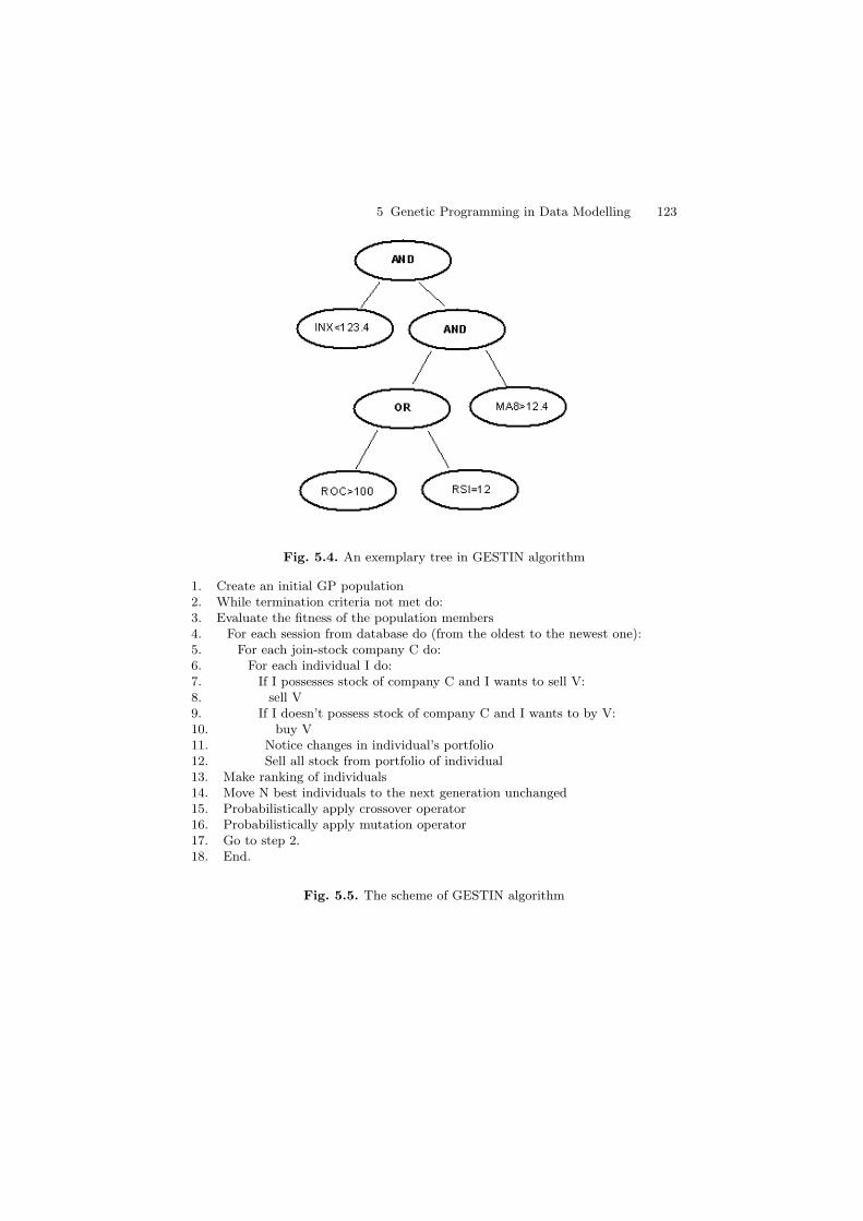
5 Genetic Programming in Data Modelling 123
Fig. 5.4. An exemplary tree in GESTIN algorithm
1. Create an initial GP population2. While termination criteria not met do:3. Evaluate the fitness of the population members4. For each session from database do (from the oldest to the newest one):5. For each join-stock company C do:6. For each individual I do:7. If I possesses stock of company C and I wants to sell V:8. sell V9. If I doesn’t possess stock of company C and I wants to by V:10. buy V11. Notice changes in individual’s portfolio12. Sell all stock from portfolio of individual13. Make ranking of individuals14. Move N best individuals to the next generation unchanged15. Probabilistically apply crossover operator16. Probabilistically apply mutation operator17. Go to step 2.18. End.
Fig. 5.5. The scheme of GESTIN algorithm

124 Halina Kwasnicka and Ewa Szpunar-Huk
needs closer insight. An individual is allowed to speculate on the stock ex-change by buying and selling stocks securities sequentially starting with anempty portfolio for data from each session in database from the oldest tothe newest session. Finally, all stocks are sold and ranking of individuals isperformed according to gain or loss given strategy brought. As the specu-lation process in reality is very complex, some restriction and simplificationare applied during the evaluation process. An individual can’t buy stock ofcompany he already possesses. The size of individual’s portfolio is set in ad-vance. Additionally, each individual has the same amount of ready cash (rc)at the beginning and maximal number of possible companies (nc) is set, butan individual can spend on stock of one company only rc/nc of cash it has atthe beginning, to insert portfolio’s diversification. To make speculation morerealistic a commission of stockbroker parameter is added, which significantlyaffect the value of the fitness function.
It is not difficult to create strategy, which is very good for data, it waslearn on. It is difficult to create a strategy earning regardless of time period.To check prediction ability of models obtained by GESTIN, some experimentswere performed. Firstly 4 different time periods were chosen: one learning –T1 and tree testing – T2, T3 and T4. These periods are characterised bydifferent WIG index values. The first one – the learning period – is a time ofbull market (WIG=+13%), the second is a time of bear market (WIG=–28%),the third one is a mixed period of bull market and bear market (WIG=0%),and the last one is a bear market with elements of bull market. Index WIG isthe main index in Warsaw Stock Exchange, and it reflects results potentiallyobtained using the simplest strategy: ”buy and keep” consisting in buyingstock at the beginning and selling in the end. Results for using 10 differentobtained strategies to the 4 time periods are shown in table 5.5.
Table 5.5. Results of 10 different strategies for one learning and three testing timeperiods of different value of WIG index
T1 T2 T3 T4WIG +13% –28% +0% –8.9%
Strategy 1 +23% –15% +0.8% +6.8%Strategy 2 +21% –23% –4% +10%Strategy 3 +21% –23% –4% +4.8%Strategy 4 +19.4% –22% –20.7% +4.4%Strategy 5 +25% –23% +2.8% +7.4%Strategy 6 +18% –15% –16% +3.6%Strategy 7 +21.6% –3.2% +10% –8.4%Strategy 8 +21.6% –21.2% –4% +11.6%Strategy 9 +19.5% –11% +9.1% +2.6%Strategy 10 +23.8% –16% +4.5% +5.5%Average +21% –19% –2 % +5%

5 Genetic Programming in Data Modelling 125
Experimental results turned out to be quite good. Except from the timeperiod T3 average results are better than index WIG. But the strategies arefar away from allowing gain during bear market. The best one seems to bethe 9-th strategy, which has quite simple and short notation:
Selling tree: MACD12<-3.8394Buying tree : (WOL<-14882 OR RSI<14.43) OR FE>3.3286e+08
5.4.3 Hybrid GP and GA to Develope Solar Cycle’s Model
The next example shows how the hybrid GP+AG algorithm for mathematicalmodelling (described in section 5.2.2) can be used to inferring models basedon time series data. The algorithm was used to develope solar cycle’s modeland experiments concerned both approximating and predicting abilities of thealgorithm were conducted.
Sunspots appear as dark spots on the surface of Sun. They typically lastfor several days, although very large ones may live for several weeks. It isknown for over 150 years that sunspots appear in cycles. The average numberof visible sunspots varies over time, increasing and decreasing on a regularcycle of between 9.5 to 11 years, on average about 10.8 years. The part of thecycle with low sunspot activity is referred to as ”solar minimum” while theportion of the cycle with high activity is known as ”solar maximum”. Thenumber of sunspots during solar maximum various for cycle to cycle. Theyare collected for about 200 years. Changes in the sun activity are shown inFig. 5.6. Knowledge of solar activity levels is often required years in advance,e.g., during satellite orbits and space missions planning [20].
Fig. 5.6. Changes in Sun activity
To run the algorithm, originally daily collected data had to be specificallytransformed into database suited to the GP. General way in which trainingand test data were generated is presented in Fig. 5.7. Firstly the learningtime period (t0, t1), the number of attributes n, and time period length d1
is determined. Attribute values are sum of sunspots appearing during timeperiod of length d1. Sunspot number for attribute y is counted for time periodlength d2, different or equal to d1, see Fig. 5.7a). Additionally distance p,

126 Halina Kwasnicka and Ewa Szpunar-Huk
denoted distance between time periods used to value of nth attribute and y, isset. According to this, if s(tp, tk) means sunspots number for the time period(tp, tk), where tp is the initial and tk the final date, for the learning time period(t0, t1) attribute values for the first training sample in database is as follows:x1 = s(t0, (t0 + d1)),x2 = s((t0 + d1), (t0 + 2d1)), ...,xn = s((t0 + (n − 2)d1), (t0 + (n − 1)d1)),y = s((t0 + (n − 1)d1 + p), (t0 + (n − 1)d1 + p + d2))The second training sample is generated similarly, but t0 gets value t0 + d1.The last kth sample is the one for which y is set for time period (t1, t1 + d2).Training database is generated in the same way but the initial test sample isthe one with first attribute value counted for a time period (t1, t1 + d2), andd1, d2, n, p parameters remind unchanged.
Fig. 5.7. Data preprocessing
In short term tests approximation turned out to be very good. Fig. 5.8and 5.9 show results of two short-time experiments (for different values ofparameters) as a comparison between value of an attribute y of given samplesfrom training set and value calculated with obtained model. Evolution wasled during 900 generations. In long-term tests approximation differed from onetime period to another but was still surprisingly good. The best approximationfor the given values of parameters (presented in Fig. 5.10) was obtained ford1 = d2 = 180 days, p = 900 days and learning time period from 1914 to 1980year. Average percentage error obtained during this experiment was equal16.9%.
Although derived functions well reflected relationships between data, theyturned out to be useless at predicting future values of solar activity both inshort and long advance. Increasing number of attributes to 30-40 and length-ening the learning time period could probably improve predicting abilities,but in the case of solar activity, it is not possible due to lack of data collectingin previous centuries.
Described experiments showed that GP algorithm can perform well in real-data, time series modelling. But the prediction task, often much more useful

5 Genetic Programming in Data Modelling 127
Fig. 5.8. Sunspot approximation – short-time test
Fig. 5.9. The best approximation of sunspots – short-time test
and desired, is however much more difficult and data-dependent, so in thiscase the GP algorithm failed.
5.4.4 General Remarks
Advances in data collection methods, storage and processing technologies areprovided a unique challenge and opportunity for automated data explorationtechniques. Enormous amounts of data are being collected periodically: daily,weekly, monthly from great scientific projects like the Human Genome Project,the Hubble Space Telescope, from stock trading, from computerised sales andother sources. GP was applied to variety of time series modelling problems forunderstanding the dynamics of natural systems or/and for decision supportsystems development.

128 Halina Kwasnicka and Ewa Szpunar-Huk
Fig. 5.10. The best approximation of sunspots – long-time test
Each approach demanded introducing of special elements to the standardGP algorithm. As an example could be mentioned Bhattacharyya, Pictet,and Zumbach work, who induce trading decision models from high-frequencyforeign exchange FX markets data. They suggested incorporation of domain-related knowledge and semantic restriction to enhance GP search. Their trad-ing model seeks to capture market movement patterns and thereby providestrading recommendations in the form of signals, a ” 1” indicating a buy sig-nal, ” –1” a sell signal, and ”0” indicating to stay out of the market [21].Another example in financial domain is Doherty’s system. Doherty appliedGP for induction of useful classification rules from the Standard and PoorsCOMPUSTAT database, which contains 334 attributes, spanning 50 years ofdata for nearly 10,000 active (trading on public markets) and 11,000 inactive(non-trading, acquired, or failed) public companies from North America. Hetransformed and normalised the database for better performance of evolutionprocess [23]. GP was also used in non-financial domains, for example to eco-logical time series analysis. Whigham’s and Recknagel’s work on applying theGrammar Based Genetic Programming framework for the discovery of pre-dictive equations and rules for phytoplankton abundance in freshwater lakesfrom time series data. They have demonstrated that models can be developedfor the non-linear dynamics of phytoplankton, both as a set of rules and asmathematical equations [23].
But, what can be noticed analysing existing approaches, it is easy to ob-tain model exactly (or almost exactly) reflecting relationships hidden in thetraining database, but in a case of predicting – accuracy of obtained models”good results” are consider to be those, for which prediction on the validationset is even slightly more right than wrong. This shows how difficult predictiontask is, and how much further work is needed.

5 Genetic Programming in Data Modelling 129
5.5 Summary
In the chapter we can see usefulness of Genetic Programming for solving se-lected problems. These problems are connected with data processing – math-ematical modelling the numerical data, classification task on the basis of pos-sessed examples, prediction and time series modelling. The problems are notnew ones, but still there are not commonly accepted methods for solving them.Genetic Programming is one of valuable approaches for them. In the mathe-matical modelling, described in section 5.2, the hybrid method – the GeneticProgramming for trees developing and the classical Genetic Algorithm for pa-rameters tuning – work together manifesting their high usefulness. The samemethod used for time series modelling (section 5.4) works very well for dataapproximation but the prediction of Sun spots is too difficult. We do notknow, if there exists a solution of this problem, it is possible that this prob-lem cannot be solved on the basis of earlier data or proposed representationof individuals.
Of course, one can find a lot of different applications of GP to data mod-elling. The authors try to select the interesting ones, showing different prob-lems with using GP. As it is known, the GP is able to solve real problems– see work of Koza, e.g., aerial designed using GP is patented. But, as it ischaracteristic for all metaheuristics, every using of such approaches must bevery carefully tuned for the solved problem. The readers are asked do notuse any ’proper’ values of parameters and genetic operators, it is necessary todevelop the proper ones for the considered problem.
References
1. Keijzer M (2002), Scientific Discovery Using Genetic Programming. PhD The-sis, Danish Technical University, Lyngby
2. Koza JR (1992), Genetic Programming: On the Programming of Computers byMeans of Natural Selection. MIT Press 106
3. Koza JR (1991), A genetic approach to econometric modelling. In: Bourgine P,Walliser B (eds), Economics and Cognitive Science. Pergamon Press, Oxford 106
4. Montana DJ (1995), Strongly typed genetic programming. Evolutionary Com-putation 3(2):199-230 114
5. Raidl GR (1998), A Hybrid GP Approach for Numerically Robust SymbolicRegression. Proc. of the 1998 Genetic Programming Conference, Madison,Wisconsin 108, 115
6. Sugimoto M, Kikuchi S, Tomita M (2003), Prediction of Biochemical ReactionsUsing Genetic Programming. Genome Informatics 14: 637-638 108
7. Langdon WB, Barrett SJ (2004), Genetic Programming in Data Mining forDrug Discovery. In: Ghosh A, Jain LC (eds), Evolutionary Computing in DataMining. Springer 114
8. Makarov DE, Metiu H (2000), Using Genetic Programming To Solve theSchrodinger Equation. The Journal of Physical Chemistry A 104 8540-8545 114

130 Halina Kwasnicka and Ewa Szpunar-Huk
9. Turton I, Openshaw S, Diplock G (1996), Some Geographical Applications ofGenetic Programming on the Cray T3D Supercomputer. Proc. of UKPAR’96,Jessope, Shafarenko (eds) 114
10. Freitas AA (2002), Data Mining and Knowledge Discovery with EvolutionaryAlgorightms. Springer-Verlag 114
11. Mallinson H, Bentley P (1999), Evolving Fuzzy Rules for Pattern Classification.Computational Integration for Modelling. Control and Automation ’99, MasoudMohammadian, IOS Press 115, 116
12. Bojarczuk CE, Lopes HS, Freitas AA (2001), Data mining with constrained-syntax genetic programming: applications in medical data sets. Proc. IntelligentData Analysis in Medicine and Pharmacology, London 116
13. Koza JR (1991), Concept formation and decision tree induction using the ge-netic programming paradigm. In: Schwefel H P, Mnner R (eds), Parallel Prob-lem Solving from Nature. Springer-Verlag, Berlin 116, 120
14. Freitas AA (2002), A survey of evolutionary algorithms for data mining andknowledge discovery. Ghosh A, Tsutsui S. (eds.) Advances in EvolutionaryComputation. Springer-Verlag
15. Noda E, Freitas AA, Lopes HS (1999), Discovering interesting prediction ruleswith a genetic algorithm. Conference Evolutionary Computation (CEC-99),Washington 116, 117
16. Ross J, Fueten F, Yashkir DY (2001), Automatic mineral identification usinggenetic programming. Machine Vision and Applications 13: 61-69, Springer-Verlag 117
17. Thompson S, Fueten F, Bockus D (2001), Mineral identification using artificialneural networks and the rotating polarizer stage. Comput Geosci, PergamonPress 117, 119
18. Gray HF, Maxwell RJ, Martinez-Perez I, Arus C, Cerdan S (1996), Geneticprogramming for classification of brain tumours from nuclear magnetic reso-nance biopsy spectra. In: Koza J R, Goldberg D E, Fogel D B, Riolo R L (eds),Proc. of the First Annual Conference, Stanford University, MIT Press 119
19. Bentley PJ (2000), ”Evolutionary, my dear Watson” – investigating committee-based evolution of fuzzy rules for the detection of suspicious insurance claims.Proc. Genetic and Evolutionary Computation Conf. (GECCO-2000), MorganKaufmann 120
20. Kippenhahn R (1994), Discovering the Secrets of the Sun. John Wiley & Sons 117, 12021. Bhattacharyya S, Pictet O V, Zumbach G (2002), Knowledge-Intensive Genetic
Discovery in Foreign Exchange Markets. IEEE Transactions on EvolutionaryComputation 125
22. Doherty CG (2003), Fundamental Analysis Using Genetic Programming forClassification Rule Induction. Genetic Algorithms and Genetic Programmingat Stanford 2003, Stanford Bookstore 128
23. Whigham PA, Recknagel F (2001), An Inductive Approach to Ecological TimeSeries Modelling by Evolutionary Computation. Ecological Modelling
24. Szpunar E (2001), Data mining methods in prediction of changes in solar ac-tivity (in polish). MA Thesis, Wroclaw University of Technology 128
25. Myszkowski PB (2002), Data mining methods in stock market analysis (inpolish). MA Thesis, Wroclaw University of Technology 108
122

6
Stock Market ModelingUsing Genetic Programming Ensembles
Crina Grosan1 and Ajith Abraham2
1 Department of Computer Science, Faculty of Mathematics and ComputerScience, Babes Bolyai University, Kogalniceanu 1, Cluj-Napoca, 3400, [email protected], http://www.cs.ubbcluj.ro/ cgrosan
2 School of Computer Science and Engineering, Chung-Ang University, 221,Heukseok-Dong, Dongjak-Gu, Seoul 156-756, [email protected], http://ajith.softcomputing.net
The use of intelligent systems for stock market predictions has been widelyestablished. This chapter introduces two Genetic Programming (GP) tech-niques: Multi-Expression Programming (MEP) and Linear Genetic Program-ming (LGP) for the prediction of two stock indices. The performance isthen compared with an artificial neural network trained using Levenberg-Marquardt algorithm and Takagi-Sugeno neuro-fuzzy model. We consideredNasdaq-100 index of Nasdaq Stock Market and the S&P CNX NIFTY stockindex as test data. Empirical results reveal that Genetic Programming tech-niques are promising methods for stock prediction. Finally formulate an en-semble of these two techniques using a multiobjective evolutionary algorithm.Results obtained by ensemble are better than the results obtained by eachGP technique individually.
6.1 Introduction
Prediction of stocks is generally believed to be a very difficult task. The processbehaves more like a random walk process and time varying. The obvious com-plexity of the problem paves way for the importance of intelligent predictionparadigms. During the last decade, stocks and futures traders have come torely upon various types of intelligent systems to make trading decisions [1],[2], [7]. This chapter presents a comparison of two genetic programming tech-niques (MEP and LGP), an ensemble MEP and LGP, artificial neural networkand a neuro-fuzzy system for the prediction of two well-known stock indicesnamely Nasdaq-100 index of NasdaqSM [19] and the S&P CNX NIFTY stockindex [20]. Nasdaq-100 index reflects Nasdaq’s largest companies across major
C. Grosan and A. Abraham: Stock Market Modeling Using Genetic Programming Ensembles,Studies in Computational Intelligence (SCI) 13, 131–146 (2006)www.springerlink.com c© Springer-Verlag Berlin Heidelberg 2006

132 Grosan and Abraham
industry groups, including computer hardware and software, telecommunica-tions, retail/wholesale trade and biotechnology [21]. The Nasdaq-100 index is amodified capitalization-weighted index, which is designed to limit dominationof the Index by a few large stocks while generally retaining the capitalizationranking of companies. Through an investment in Nasdaq-100 index trackingstock, investors can participate in the collective performance of many of theNasdaq stocks that are often in the news or have become household names.Similarly, S&P CNX NIFTY is a well-diversified 50 stock index accountingfor 25 sectors of the economy [13]. It is used for a variety of purposes suchas benchmarking fund portfolios, index based derivatives and index funds.The CNX Indices are computed using market capitalisation weighted method,wherein the level of the Index reflects the total market value of all the stocksin the index relative to a particular base period. The method also takes intoaccount constituent changes in the index and importantly corporate actionssuch as stock splits, rights, etc without affecting the index value.
MEP and LGP techniques are applied for modeling the Nasdaq-100 andNIFTY stock market indices so as to optimize the performance indices (dif-ferent error measures, correlation coefficient and so on). Results obtained byMEP and LGP are compared with the results obtained using an artificialneural network trained using the Levenberg-Marquardt algorithm [5] and aTakagi-Sugeno fuzzy inference system learned using a neural network algo-rithm (neuro-fuzzy model) [3][15]. Neural networks are excellent forecastingtools and can learn from scratch by adjusting the interconnections betweenlayers. Neuro-fuzzy computing is a popular framework wherein neural networktraining algorithms are used to fine-tune the parameters of fuzzy inferencesystems. We will build an ensemble between MEP and LGP using a multiob-jective evolutionary algorithm (Non-dominated Sorting Genetic Algorithm II(NSGAII)). Results obtained by ensemble are then compared with the resultsobtained by MEP and LGP individually.
In Section 6.1, we briefly describe the stock marketing modeling problem.In Section 6.2, different connectionist paradigms used in experiments are pre-sented. In Section 6.3, we formulate the ensemble between MEP and LGPfollowed by experimentation setup in Section 6.4 and results in Section 6.5.Some conclusions are also provided towards the end.
6.2 Modeling Stock Market Prediction
We analysed the Nasdaq-100 index value from 11 January 1995 to 11 January2002 [19] and the NIFTY index from 01 January 1998 to 03 December 2001[20]. For both indices, we divided the entire data into almost two equal parts.No special rules were used to select the training set other than ensuring areasonable representation of the parameter space of the problem domain. Thecomplexity of the training and test data sets for both indices are depicted inFigures 6.1 and 6.2 respectively.

6 Stock Modeling Using GP Ensembles 133
Fig. 6.1. Training and test data sets for Nasdaq-100 Index
Fig. 6.2. Training and test data sets for NIFTY index
Our goal is to optimize several error measures: Root Mean Squared Error(RMSE), Correlation Coefficient (CC), Maximum Absolute Percentage Error(MAP) and Mean Absolute Percentage Error (MAPE):

134 Grosan and Abraham
RMSE =
√√√√N∑
i=1
|Pactual,i − Ppredicted,i| (6.1)
CC =
N∑i=1
Ppredicted,i
N∑i=1
Pactual,i
, (6.2)
MAP = max( |Pactual, i − Ppredicted, i|
Ppredicted, i× 100
)(6.3)
MAPE =1N
N∑
i=1
[ |Pactual, i − Ppredicted, i|Pactual, i
]× 100, (6.4)
where Pactual,i is the actual index value on day i, Ppredicted,i is the forecastvalue of the index on that day and N = total number of days. The task is tohave minimal values of RMSE, MAP and MAPE and a maximum value forCC.
6.3 Intelligent Paradigms
The different paradigms used in this chapter are described in this Section.
6.3.1 Multi Expression Programming (MEP)
MEP is a Genetic Programming variant that uses a linear representation ofchromosomes. MEP individuals are strings of genes encoding complex com-puter programs. When MEP individuals encode expressions, their representa-tion is similar to the way in which compilers translate C or Pascal expressionsinto machine code [4].
A unique MEP feature is the ability of storing multiple solutions of aproblem in a single chromosome. Usually, the best solution is chosen for fit-ness assignment. When solving symbolic regression or classification problems(or any other problems for which the training set is known before the problemis solved) MEP has the same complexity as other techniques storing a singlesolution in a chromosome (such as Genetic Programming [17], Cartesian Ge-netic Programming [18], Gene Expression Programming [11] or GrammaticalEvolution [24]).
Evaluation of the expressions encoded into a MEP individual can be per-formed by a single parsing of the chromosome.
Offspring obtained by crossover and mutation are always syntactically cor-rect MEP individuals (computer programs). Thus, no extra processing for re-pairing newly obtained individuals is needed. (For technical details, the readeris advised to refer to the chapter on Evolving Intrusion Detection Systems orsee [22].)

6 Stock Modeling Using GP Ensembles 135
6.3.2 Linear Genetic Programming (LGP)
Linear genetic programming is a variant of the GP and is throughly describedin chapter on Evolving Intrusion Detection Systems. LGP uses a specific lin-ear representation of computer programs. Instead of the tree-based GP ex-pressions of a functional programming language (like LISP) programs of animperative language (like C) are evolved.
An LGP individual is represented by a variable-length sequence of simpleC language instructions. Instructions operate on one or two indexed variables(registers) r, or on constants cfrom predefined sets. The result is assigned to adestination register, for example, ri = rj* c. Here is an example LGP program:
void LGP(double v[8]) v[0] := v[5] + 73;v[7] := v[3] – 59;if (v[1] > 0)if (v[5] > 21)v[4] := v[2] .v[1];v[2] := v[5] + v[4];v[6] := v[7] .25;v[6] := v[4] – 4;v[1] := sin(v[6]);if (v[0] > v[1])v[3] := v[5] .v[5];v[7] := v[6] .2;v[5] := v[7] + 115;if (v[1] ≤ v[6])v[1] := sin(v[7]);
A LGP can be turned into a functional representation by successive re-placements of variables starting with the last effective instruction. The maxi-mum number of symbols in a LGP chromosome is 4 * Number of instructions.Evolving programs in a low-level language allows us to run those programsdirectly on the computer processor, thus avoiding the need of an interpreter.In this way the computer program can be evolved very quickly.
An important LGP parameter is the number of registers used by a chromo-some. The number of registers is usually equal to the number of attributes ofthe problem. If the problem has only one attribute, it is impossible to obtaina complex expression such as the quartic polynomial. In that case we have touse several supplementary registers. The number of supplementary registersdepends on the complexity of the expression being discovered.
An inappropriate choice can have disastrous effects on the program beingevolved.

136 Grosan and Abraham
LGP uses a modified steady-state algorithm. The initial population is ran-domly generated. The following steps are repeated until a termination cri-terion is reached: Four individuals are randomly selected from the currentpopulation. The best two of them are considered the winners of the tourna-ment and will act as parents. The parents are recombined and the offspringare mutated and then replace the losers of the tournament.
We used a LGP technique that manipulates and evolves a program at themachine code level. The settings of various linear genetic programming sys-tem parameters are of utmost importance for successful performance of thesystem. The population space has been subdivided into multiple subpopu-lation or demes. Migration of individuals among the sub-populations causesevolution of the entire population. It helps to maintain diversity in the pop-ulation, as migration is restricted among the demes. Moreover, the tendencytowards a bad local minimum in one deme can be countered by other demeswith better search directions. The various LGP search parameters are themutation frequency, crossover frequency and the reproduction frequency: Thecrossover operator acts by exchanging sequences of instructions between twotournament winners. Steady state genetic programming approach was used tomanage the memory more effectively.
6.3.3 Artificial Neural Network (ANN)
The artificial neural network methodology enables us to design useful nonlin-ear systems accepting large numbers of inputs, with the design based solelyon instances of input-output relationships. For a training set T consisting ofnargument value pairs and given a d-dimensional argument x and an associ-ated target value t will be approximated by the neural network output. Thefunction approximation could be represented as
T = (xi, ti) : i = 1 : n (6.5)
In most applications the training set T is considered to be noisy and ourgoal is not to reproduce it exactly but rather to construct a network functionthat generalizes well to new function values. We will try to address the problemof selecting the weights to learn the training set. The notion of closeness onthe training set T is typically formalized through an error function of the form
ψT =n∑
i=1
‖ yi − ti ‖2 (6.6)
where yi is the network output.
Levenberg-Marquardt Algorithm
The Levenberg-Marquardt (LM) algorithm [5] exploits the fact that the errorfunction is a sum of squares as given in (6.6). Introduce the following notation

6 Stock Modeling Using GP Ensembles 137
for the error vector and its Jacobian with respect to the network parametersw
J = Jij =∂ej
∂wi, i = 1 : p, j = 1 : n (6.7)
The Jacobian matrix is a large p × n matrix, all of whose elements arecalculated directly by backpropagation technique. The p dimensional gradientg for the quadratic error function can be expressed as:
g(w) =n∑
i=1
ei∇ei(w) = Je (6.8)
and the Hessian matrix by:
H = Hij = ∂2ψT
∂wi∂wj
= 12
n∑k=1
∂2e2k
∂wi∂wj=
n∑k=1
(ek
∂2ek
∂wi∂wj+∂2ek
∂wi∂wj
)
=n∑
k=1
(ek
∂2ek
∂wi∂wj+ JikJjk
)(6.9)
Hence defining D =n∑
i=1
ei∇2eiyields the expression
H(w) = JJT + D (6.10)
The key to the LM algorithm is to approximate this expression for theHessian by replacing the matrix D involving second derivatives by the muchsimpler positively scaled unit matrix ∈ I. The LM is a descent algorithm usingthis approximation in the form below:
Mk =[JJT + ∈ I
]−1, wk+1 = wk − αkMkg(wk) (6.11)
Successful use of LM requires approximate line search to determine the rateαk. The matrix JJT is automatically symmetric and non-negative definite.The typically large size of J may necessitate careful memory managementin evaluating the product JJT . Hence any positive ∈ will ensure that Mk ispositive definite, as required by the descent condition. The performance of thealgorithm thus depends on the choice of ∈.
When the scalar ∈ is zero, this is just Newton’s method, using the ap-proximate Hessian matrix. When ∈ is large, this becomes gradient descentwith a small step size. As Newton’s method is more accurate, ∈ is decreasedafter each successful step (reduction in performance function) and is increasedonly when a tentative step would increase the performance function. By doingthis, the performance function will always be reduced at each iteration of thealgorithm.

138 Grosan and Abraham
6.3.4 Neuro-Fuzzy System
Neuro Fuzzy (NF) computing is a popular framework for solving complexproblems [3]. If we have knowledge expressed in linguistic rules, we can builda Fuzzy Inference System (FIS) [8], and if we have data, or can learn froma simulation (training) then we can use ANNs. For building a FIS, we haveto specify the fuzzy sets, fuzzy operators and the knowledge base. Similarlyfor constructing an ANN for an application the user needs to specify thearchitecture and learning algorithm. An analysis reveals that the drawbackspertaining to these approaches seem complementary and therefore it is naturalto consider building an integrated system combining the concepts. While thelearning capability is an advantage from the viewpoint of FIS, the formationof linguistic rule base will be advantage from the viewpoint of ANN. Figure6.3 depicts the 6-layered architecture of multiple output neuro-fuzzy systemimplementing a Takagi-Sugeno fuzzy inference system. For technical details,the reader is advised to consult [15].
Fig. 6.3. Architecture of ANFIS
6.4 Ensemble of GP Techniques
Our goal is to optimize four error measures namely Root Mean Squared Er-ror (RMSE), Correlation Coefficient (CC), Maximum Absolute Percentage

6 Stock Modeling Using GP Ensembles 139
Error(MAP) and Mean Absolute Percentage Error (MAPE). The task is tohave minimal values of RMSE, MAP, MAPE and a maximum value for CC.The objective is to carefully construct the different GP models to achieve thebest generalization performance. Test data is then passed through these in-dividual models and the corresponding outputs are recorded. Suppose resultsobtained by LGP and MEP are anand bn respectively and the correspondingdesired value is xn. The task is to combine an andbn so as to get the bestoutput value that maximizes the CC and minimizes the RMSE, MAP andMAPE values.
We consider this problem as a multiobjective optimization problem inwhich we want to find solution of this form: (coef 1, coef 2) where coef 1, andcoef 2 are real numbers between -1 and 1, so as the resulting combination:
coef1 ∗ an + coef2 ∗ bn (6.12)
would be close to the desired value xn. This means, in fact, to find a solutionso as to simultaneously optimize RMSE, MAP, MAPE and CC. This problemis equivalent to finding the Pareto solutions of a multiobjective optimizationproblem. For this problem, the objectives are RMSE, MAP, MAPE and CC.We use the well known Multiobjective Evolutionary Algorithm (MOEA) -Nondominated Sorting Genetic Algorithm II (NSGAII) [10] and a short de-scription of this algorithm is given in the subsequent Section.
6.4.1 Nondominated Sorting Genetic Algorithm II (NSGA II)
In the Nondominated Sorting Genetic Algorithm (NSGA II)[10] for each so-lution x the number of solutions that dominate solution x is calculated. Theset of solutions dominated by x is also calculated. The first front (the currentfront) of the solutions that are nondominated is obtained.
Let us denote by Si the set of solutions that are dominated by the solutionxi. For each solution xi from the current front consider each solution xq fromthe set Si.
The number of solutions that dominates xqis reduced by one. The solutionswhich remain non-dominated after this reduction will form a separate list.This process continues using the newly identified front as the current front.Let P (0) be the initial population of size N . An offspring population Q(t)of size N is created from current population P (t). Consider the combinedpopulation R(t) = P(t) ∪Q(t).
Population R(t) is ranked according to nondomination. The fronts F1,F2, . . . are obtained. New population P (t+1) is formed by considering indi-viduals from the fronts F1, F2, ..., until the population size exceeds N. Solu-tions of the last allowed front are ranked according to a crowded comparisonrelation.
NSGA II uses a parameter (called crowding distance) for density estima-tion for each individual. Crowding distance of a solution x is the average

140 Grosan and Abraham
side-length of the cube enclosing the point without including any other pointin the population. Solutions of the last accepted front are ranked accordingto the crowded comparison distance
NSGA II works follows. Initially a random population, which is sortedbased on the nondomination, is created. Each solution is assigned a fitnessequal to its nondomination level (1 is the best level). Binary tournament selec-tion, recombination and mutation are used to create an offspring population.A combined population is formed from the parent and offspring population.The population is sorted according to the nondomination relation. The newparent population is formed by adding the solutions from the first front andthe followings until exceed the population size. Crowding comparison proce-dure is used during the population reduction phase and in the tournamentselection for deciding the winner.
6.5 Experiment Results
We considered 7 year’s month’s stock data for Nasdaq-100 Index and 4 year’sfor NIFTY index. Our target is to develop efficient forecast models that couldpredict the index value of the following trading day based on the opening,closing and maximum values of the same on a given day. For the Nasdaq-100index the data sets were represented by the ‘opening value’, ‘low value’and ‘high value’. NIFTY index data sets were represented by ‘opening value’,‘low value’, ‘high value’ and ‘closing value’. The assessment of the predic-tion performance of the different connectionist paradigms and the ensemblemethod were done by quantifying the prediction obtained on an independentdata set.
6.5.1 Parameter Settings
MEP Parameter Settings. Parameters used by MEP in these experimentsare presented in Table 6.1. Next two experiments analyze the results obtainedby MEP by considering different population sizes and different values for chro-mosome length. The values for the other parameters are adapted from Table6.1. Population size was considered 150 for both test data. Average resultsobtained from 10 different runs and the best results obtained are presented inTable 6.2. Results obtained for different population sizes and various chromo-some lengths are presented in Tables 6.3 and 6.4 respectively for both Nasdaqand Nifty test data.
As evident from Table 6.2 the best results for Nasdaq is obtained using apopulation of 100 individuals and for Nifty using a population of 150 individ-uals. Table 6.3 illustrates that the best result for both Nasdaq and Nifty isobtained using a chromosome length of 40 and 50.

6 Stock Modeling Using GP Ensembles 141
Table 6.1. Values of parameters used by MEP
Parameter Value
Population sizeNasdaq 100Nifty 50
Number of iterationNasdaq 60Nifty 100
Chromosome lengthNasdaq 30Nifty 40
Crossover Probability 0.9
Functions set +, - , *, /, sin,cos, sqrt, ln, lg, log2,min, max, abs
Table 6.2. Performance measures obtained by MEP or population sizes
Population size50 100 150 200
Nasdaq
RMSEBest 0.022 0.032 0.035 0.0168Average 0.024 0.027 0.03 0.022
CCBest 0.999 0.097 0.97 0.992Average 0.995 0.984 0.98 0.997
MAPBest 97.43 103.31 103.31 103.31Average 109.59 100.37 109.33 100.7
MAPEBest 18.13 9.02 9.08 8.69Average 23.32 13.58 18.8 18.23
Nifty
RMSEBest 0.0187 0.163 0.015 0.0138Average 0.02 0.0196 0.0197 0.019
CCBest 0.999 0.997 0.999 0.999Average 0.991 0.979 0.978 0.988
MAPBest 38.99 31.7 27.64 30.03Average 53.02 42.225 41.85 48.81
MAPEBest 4.131 3.72 3.17 3.027Average 4.9 4.66 4.81 4.34
LGP Parameter Settings. Parameters values used by LGP for Nasdaq andNifty test data are presented in Table 6.4.
Ensemble Using NSGAII Parameter Setting. Parameters values usedby NSGAII for combining (ensembling) MEP and LGP are given in Table 6.5.These parameters were used for both Nasdaq and Nifty test data.
ANN and NF parameter settings. We used a feed forward neural net-work with 4 input nodes and a single hidden layer consisting of 26 neurons.Tanh-sigmoidal activation function was for the hidden neurons. The trainingusing LM algorithm was terminated after 50 epochs and it took about 4 sec-

142 Grosan and Abraham
Table 6.3. Performance measures obtained by MEP for different chromosomelengths
Chromosome length20 30 40 50
Nasdaq
RMSEBest 0.021 0.032 0.028 0.0165Average 0.021 0.027 0.024 0.022
CCBest 0.998 0.976 0.977 0.993Average 0.998 0.987 0.985 0.994
MAPBest 97.43 103.31 103.31 103.31Average 97.43 100.38 118.5 115.55
MAPEBest 18.11 9.02 8.91 8.53Average 18.12 13.52 18.74 15.86
Nifty
RMSEBest 0.0187 0.0169 0.015 0.014Average 0.0193 0.023 0.0197 0.02
CCBest 0.999 0.990 0.999 0.992Average 0.994 0.977 0.98 0.981
MAPBest 38.99 42.98 27.64 34.87Average 43.37 52.1 38.78 40.67
MAPEBest 4.125 4.08 3.17 3.30Average 4.33 5.68 4.81 4.75
Table 6.4. LGP parameter settings
Parameter Value
Population size 100
Mutation frequency 95%
Crossover frequency 50%
Number of demes 10
Number of constants 60
Table 6.5. Parameters values used by NSGAII for ensembling MEP and LGP
Parameter Value
Population size 250
Mutation probability 0.3
Crossover probability 0.5
Number of generations 1,000
Chromosome length 30

6 Stock Modeling Using GP Ensembles 143
onds to train each dataset. For the neuro-fuzzy system, we used 3 triangularmembership functions for each of the input variable and the 27 if-then fuzzyrules were learned for the Nasdaq-100 index and 81 if-then fuzzy rules for theNIFTY index. Training was terminated after 12 epochs and it took about 3seconds to train each dataset [1].
6.5.2 Comparisons of Results Obtained by Intelligent Paradigms
Table 6.6 summarizes the results achieved for the two stock indices using thefive intelligent paradigms (ANN, NF, MEP, LGP and the ensemble betweenLGP and MEP).
Table 6.6. Results obtained by intelligent paradigms for Nasdaq and Nifty testdata
ANN NF MEP LGP Ensemble
Test results for Nasdaq
RMSE 0.0284 0.0183 0.021 0.021 0.0203
CC 0.9955 0.9976 0.999 0.9940 1.000
MAP 481.71 520.84 97.39 97.94 96.92
MAPE 9.032 7.615 14.33 19.65 19.25
Test results for Nifty
RMSE 0.0122 0.0127 0.0163 0.0124 0.0127
CC 0.9968 0.9967 0.997 0.995 1.000
MAP 73.94 40.37 31.7 40.02 31.9
MAPE 3.353 3.320 3.72 2.83 2.80
The combination obtained by ensemble between LGP and MEP are re-ported below:
Nasdaq: 0.669668 ∗ an + 0.334354 ∗ bn
Nifty: 0.632351 ∗ an + 0.365970 ∗ bn
where an and bn correspond to LGP and MEP indices respectively.As depicted in Table 6.6, for Nasdaq test data, MEP gives the best results
for MAP (97.39). Also LGP gives results very close to MEP while the othertechniques did not perform that well. While MEP obtained the best result forCC, the performance obtained were close to the results obtained for RMSEby the other paradigms. Results obtained by ensemble clearly outperformsalmost all considered techniques. For both Nasdaq and Nifty test data, thevalues obtained by the ensemble for CC is 1.000.
Since the multiobjective evolutionary algorithm was used to simultane-ously optimize all the four performance measures (RMSE, CC, MAP andMAPE), more than one solution could be obtained in the final population

144 Grosan and Abraham
(which, in fact, means more than one combination between LGP and MEP).Some examples of the solutions obtained for Nifty is given below:
• Best value for RMSE obtained by the ensemble is 0.012375, while CC =0.999, MAP = 36.86 and MAPE = 2.71.
• Best value for MAP obtained by the ensemble is 25.04, while RMSE =0.0138, CC = 0.998 and MAPE = 3.05.
• Best result obtained by the ensemble for MAPE is 2.659513, while RMSE= 0.0124, CC = 0.998 and MAP = 41.44.
6.6 Summary
In this chapter, we presented five techniques for modeling stock indices. Theperformance of GP techniques (empirical results) when compared to ANNand NF clearly indicate that GP could play a prominent role for stock marketmodeling problems. The fluctuations in the share market are chaotic in thesense that they heavily depend on the values of their immediate fore run-ning fluctuations. Our main task was to find the best values for the severalperformance measures namely RMSE, CC, MAP and MAPE. We applieda multiobjective optimization algorithm in order to ensemble the GP tech-niques. Experiment results reveal that the ensemble performs better than theGP techniques considered separately.
According to the No Free Lunch Theorem (NFL), for any algorithm, anyelevated performance over one class of problems is exactly paid for in perfor-mance over another class [26]. Taking into account of the NFL theorem, itwould be a rather difficult task to predict which paradigm would perform thebest for different stock indices [13].
Acknowledgements
This research was supported by the International Joint Research Grant ofthe IITA (Institute of Information Technology Assessment) foreign professorinvitation program of the MIC (Ministry of Information and Communication),South Korea.
References
1. Abraham, A. and AuYeung, A., Integrating Ensemble of Intelligent Systems forModeling Stock Indices, In Proceedings of 7th International Work Conferenceon Artificial and Natural Neural Networks, Lecture Notes in Computer Science-Volume 2687, Jose Mira and Jose R. Alverez (Eds.), Springer Verlag, Germany,pp. 774-781, 2003. 131, 143

6 Stock Modeling Using GP Ensembles 145
2. Abraham, A. Philip, N.S. and Saratchandran, P., Modeling Chaotic Behaviorof Stock Indices Using Intelligent Paradigms. International Journal of Neural,Parallel & Scientific Computations, USA, Volume 11, Issue (1&2) pp.143-160,2003. 131
3. Abraham, A., Neuro-Fuzzy Systems: State-of-the-Art Modeling Techniques,Connectionist Models of Neurons, Learning Processes, and Artificial Intelli-gence, Springer-Verlag Germany, Jose Mira and Alberto Prieto (Eds.), Granada,Spain, pp. 269-276, 2001. 132, 138
4. Aho, A., Sethi R., Ullman J., Compilers: Principles, Techniques, and Tools,Addison Wesley, 1986. 134
5. Bishop, C. M., Neural Networks for Pattern Recognition, Oxford: ClarendonPress, 1995. 132, 136
6. M. Brameier and W. Banzhaf, A Comparison of Linear Genetic Programmingand Neural Networks in Medical Data Mining, IEEE Transactions on Evolu-tionary Computation, 5, pp.17-26, 2001.
7. M. Brameier and W. Banzhaf, Explicit Control of Diversity and Effective Vari-ation Distance in Linear Genetic Programming,in Proceedings of the FourthEuropean Conference on Genetic Programming, edited by E. Lutton, J. Foster,J. Miller, C. Ryan, and A. Tettamanzi (Springer-Verlag, Berlin, 2002). 131
8. Cherkassky V., Fuzzy Inference Systems: A Critical Review, ComputationalIntelligence: Soft Computing and Fuzzy-Neuro Integration with Applications,Kayak O, Zadeh L A et al (Eds.), Springer, pp.177-197, 1998. 138
9. Collobert R. and Bengio S., SVMTorch: Support Vector Machines for Large-Scale Regression Problems, Journal of Machine Learning Research, Volume 1,pages 143-160, 2001.
10. Deb, K., Agrawal, S., Pratab, A., Meyarivan, T., A fast elitist non-dominatedsorting genetic algorithms for multiobjective optimization: NSGA II. KanGALreport 200001, Indian Institute of Technology, Kanpur, India, 2000. 139
11. C. Ferreira, Gene Expression Programming: A New Adaptive Algorithm forSolving Problems, Complex Systems, 13 (2001) 87-129. 134
12. E.H. Francis et al. Modified Support Vector Machines in Financial Time SeriesForecasting, Neurocomputing 48(1-4): pp. 847-861, 2002.
13. C. Grosan and A. Abraham, Solving No Free Lunch Issues from a PracticalPerspective, In Proceedings of Ninth International Conference on Cognitive andNeural Systems, ICCNS’05, Boston University Press, USA, 2005 . 132, 144
14. S. Hashem. Optimal Linear Combination of Neural Networks. Neural Network,Volume 10, No. 3. pp. 792-994, 1995.
15. J.S.R. Jang, C.T. Sun and E. Mizutani. Neuro-Fuzzy and Soft Computing: AComputational Approach to Learning and Machine Intelligence, Prentice HallInc, USA, 1997. 132, 138
16. T. Joachims . Making large-Scale SVM Learning Practical. Advances in KernelMethods - Support Vector Learning, B. Scholkopf and C. Burges and A. Smola(Eds.), MIT-Press, 1999. 68
17. J. R. Koza, Genetic Programming: On the Programming of Computers by Meansof Natural Selection (MIT Press, Cambridge, MA, 1992). 134
18. J. Miller and P. Thomson. Cartesian Genetic Programming, in Proceedings ofthe Third European Conference on Genetic Programming, edited by RiccardoPoli, Wolfgang Banzhaf, Bill Langdon, Julian Miller, Peter Nordin, and TerenceC. Fogarty (Springer-Verlag, Berlin, 2002). 134

146 Grosan and Abraham
19. Nasdaq Stock MarketSM : http://www.nasdaq.com. 131, 13220. National Stock Exchange of India Limited: http://www.nse-india.com. 131, 13221. M. Oltean and C. Grosan. A Comparison of Several Linear GP Techniques.
Complex Systems, Vol. 14, Nr. 4, pp. 285-313, 200422. M. Oltean M. C. Grosan. Evolving Evolutionary Algorithms using Multi Expres-
sion Programming. Proceedings of The 7 th European Conference on ArtificialLife, Dortmund, Germany, pp. 651-658, 2003. 134
23. N.S. Philip and K.B. Joseph. Boosting the Differences: A Fast Bayesian classifierneural network, Intelligent Data Analysis, Vol. 4, pp. 463-473, IOS Press, 2000.
24. C. Ryan C. J.J. Collins and M. O’Neill. Gramatical Evolution: Evolving pro-grams for an arbitrary language. In Proceedings of the first European Workshopon Genetic Programming, Springer-Verlag, Berlin, 1998. 134
25. R.E. Steuer. Multiple Criteria Optimization: Theory, Computation and Appli-cations. New York: Wiley, 1986
26. D.H. Wolpert and W.G. Macready. No free lunch theorem for search. TechnicalReport SFI-TR-95-02-010. Santa Fe Institute, USA, 1995. 144

7
Evolutionary Digital Circuit DesignUsing Genetic Programming
Nadia Nedjah1 and Luiza de Macedo Mourelle2
1 Department of Electronics Engineering and Telecommunications,Engineering Faculty,State University of Rio de Janeiro,Rua Sao Francisco Xavier, 524, Sala 5022-D,Maracana, Rio de Janeiro, [email protected], http://www.eng.uerj.br/~nadia
2 Department of System Engineering and Computation,Engineering Faculty,State University of Rio de Janeiro,Rua Sao Francisco Xavier, 524, Sala 5022-D,Maracana, Rio de Janeiro, [email protected], http://www.eng.uerj.br/~ldmm
In this chapter, we study two different circuit encodings used for digital cir-cuit evolution. The first approach is based on genetic programming, whereindigital circuits consist of their data flow based specifications. In this approach,individuals are internally represented by the abstract trees/DAG of the cor-responding circuit specifications. In the second approach, digital circuits arethought of as a map of rooted gates. So individuals are represented by two-dimensional arrays of cells. Each of these cells consists of the logic gate nametogether with the corresponding input signal names as the name of the outputsignal is fixed. Furthermore, we compare the impact of both individual repre-sentations on the evolution process of digital circuits. Evolved circuits shouldminimise space and time requirements. We show that for the same input/out-put behaviour, employing either of these approaches yields circuits of almostthe same characteristics in terms of space and response time. However, theevolutionary process is much shorter with the second encoding.
7.1 Introduction
evolutionary hardware [7] is a hardware that is yield using simulated evolu-tion as an alternative to conventional-based electronic circuit design. Genetic
N. Nedjah and L. de M. Mourelle: Evolutionary Digital Circuit Design Using Genetic Program-ming, Studies in Computational Intelligence (SCI) 13, 147–171 (2006)www.springerlink.com c© Springer-Verlag Berlin Heidelberg 2006

148 Nadia Nedjah and Luiza de Macedo Mourelle
evolution is a process that evolves a set of individuals, which constitutes thepopulation, producing a new population. Here, individuals are hardware de-signs. The more the design obeys the constraints, the more it is used in thereproduction process. The design constraints could be expressed in terms ofhardware area and/or response time requirements. The freshly produced pop-ulation is yield using some genetic operators such as crossover and mutationthat attempt to simulate the natural breeding process in the hope of generat-ing new design that are fitter i.e. respect more the design constraints. Geneticevolution is usually implemented using genetic algorithms.
The problem of interest consists of choosing the best encoding for evolvingrapidly efficient and creative circuits that implement a given input/outputbehaviour without much designing effort. The obtained circuits are expectedto be minimal both in terms of space and time requirements: The circuitsmust be compact i.e. use a reduced number of gates and efficient, i.e. producethe output in a short response time. The response time of a circuit dependson the number and the complexity of the gates forming the longest path init. The complexity of a gate depends solely on the number of its inputs.
The remainder of this chapter is divided in five sections. In Section 7.2,we describe the principles of evolutionary hardware. In Section 7.3, we de-scribe the first methodology and propose the necessary genetic operators. InSection 7.4, we describe the second approach as well as the corresponding ge-netic operators. In Section 7.5, we compare the evolved hardware using eithermethodologies. Finally, we draw some conclusions.
7.2 Principles of Evolutionary Hardware Design
Evolutionary hardware [7] consists simply of hardware designs evolved usinggenetic algorithms, wherein chromosomes represent circuit designs. In general,evolutionary hardware design offers a mechanism to get a computer to providea design of circuit without being told exactly how to do it. In short, it allowsone to automatically create circuits. It does so based on a high level state-ment of the constraints the yielded circuit must obey to. The input/outputbehaviour of the expected circuit is generally considered as an omnipresentconstraint. Furthermore, the generated circuit should have a minimal size.
Starting form random set of circuit design, which is generally called ini-tial population, evolutionary hardware design breeds a population of designsthrough a series of steps, called generations, using the Darwinian principle ofnatural selection. Circuits are selected based on how much they adhere to thespecified constraints. Fitter individuals are selected, recombined to produceoffspring which in turn should suffer some mutations. Such offspring are thenused to populate of the next generation. This process is iterated until a cir-cuit design that obeys to all prescribed constraints is encountered within thecurrent population.

7 Evolutionary Digital Circuit Design 149
Each circuit within the population is assigned a value, generally called fit-ness. A circuit design is it fit if and only if it satisfies the imposed input/outputbehaviour. A circuit design is considered fitter than another if and only if ithas a smaller size.
An important aspect of evolutionary hardware design is thus to provide away to evaluate the adherence of evolved circuits to the imposed constraints.These constraints are of two kinds. First of all, the evolved circuit designmust obey the input/output behaviour, which is given in a tabular form ofexpected results given the inputs. This is the truth table of the expectedcircuit. Second, the circuit must have a reduced size. This constraint allowsus to yield compact digital circuits.
We estimate the necessary area for a given circuit using the concept of gateequivalent. This is the basic unit of measure for digital circuit complexity [6].It is based upon the number of logic gates that should be interconnected toperform the same input/output behaviour. This measure is more accuratethat the simple number of gates [6]. The number of gate equivalent and anaverage propagation delay for each kind of gate are given in Table 7.1. Thedata were taken form [6]. Note that only 2-input gates not, and, or, xor,nand, nor, xnor and 2:1-mux are allowed as the complemented input signalsare available at no extra cost.
Table 7.1. Gates symbols, number of gate-equivalent
Name Code Gate-equivalent delay
not 0 1 0.0625and 1 2 0.2090or 2 2 0.2160xor 3 3 0.2120nand 4 1 0.1300nor 5 1 0.1560xnor 6 3 0.2110mux 7 3 0.2120
The xor gate is a CMOS basic gate that has the behaviour of sum ofproducts xy + xy, wherein x and y are the input signals. However, a xor
gate is not implemented using 2 and gates, 2 not gates and an or gate. A2:1-multipliexer mux is also a CMOS basic gate and implements the sum ofproducts xs + ys wherein x and y are the first and the second input signalsand s is the control signal. It is clear that a xor and mux gates are of thesame complexity [6].
Let us formalise the fitness function. For this purpose, let C be a digitalcircuit that uses a subset (or the complete set) of the gates given in Table 7.1.Let gates(C) be a function that returns the set of all gates of C. On the other

150 Nadia Nedjah and Luiza de Macedo Mourelle
hand, let val(T ) be the Boolean value that C propagates for the input Booleanvector T assuming that the size of T coincides with the number of input signalrequired for C. The fitness function is given as follows, wherein X representsthe input values of the input signals while Y represents the expected values ofthe output signals of C, n denotes the number of output signals that C has.
Let us formalise the fitness function. For this purpose, let C be a digitalcircuit that uses a subset (or the complete set) of the gates given in Table7.1. Let gates(C) be a function that returns the set of all gates of circuitC and levels(C) be a function that returns the set of all the gates of Cgrouped by level. Notice that the number of levels of a circuit coincides withthe cardinality of the set expected from function levels. On the other hand,let val(X) be the Boolean value that the considered circuit C propagates forthe input Boolean vector X assuming that the size of X coincides with thenumber of input signal required for circuit C. The fitness function, whichallows us to determine how far an evolved circuit adheres to the specifiedconstraints, is given in Equation 7.1, wherein X represents the values of theinput signals while Y represents the expected values of the output signals ofcircuit C, n denotes the number of output signals that circuit C has, functiondelay returns the propagation delay of a given gate as shown in Table 7.1and ω1 and ω2 are the weighting coefficients that allow us to consider bothhardware area and response time to evaluate the performance of an evolvedcircuit, with ω1 + ω2 = 1. For implementation issue, we minimized the fitnessfunction below for different values of ω1 and ω2.
Fitness(C) =∑n
j=1
(∑i|val(Xi) =Yi,j
penalty)
+ω1 ×∑
g∈gates(C) gateEqui(g)
+ω2 ×∑
l∈levels(C) maxg∈l delay(g)
(7.1)
For instance, consider the evolved specification of Fig. 7.1. It should prop-agate the output signals of Table 7.2 that appear first (i.e. before symbol /)but it actually propagates the output signals that appear last (i.e. those af-ter symbol /). Observe that signals Z2 and Z1 are correct for every possiblecombination of the input signals. However, signal Z0 is correct only for thecombinations 1010 and 1111 of the input signals and so for the remaining 14combinations, Z0 has a wrong value and so the circuit should be penalised 14times. Applying function gates to this circuit should return 5 and gates and 3or gates. Now applying function levels to this circuit should return two levels:and, and, or, or, or and and, and, and . If penalty is set to 10 then,function Fitness should return 140 + 0.5(5 × 2 + 3 × 1) + 0.5(0.216 + 0.209).This fitness sums up to 21.7125. Note that for a correct circuit the first termin the definition of function Fitness is zero and so the value returned by this

7 Evolutionary Digital Circuit Design 151
Table 7.2. Truth table of the circuit whose schematics are given in Fig. 7.1
X1 X0 Y1 Y0 Z2 Z1 Z0
0 0 0 0 0/0 0/0 0/10 0 0 1 0/0 0/0 0/10 0 1 0 0/0 0/0 0/10 0 1 1 0/0 0/0 0/10 1 0 0 0/0 0/0 0/10 1 0 1 0/0 0/0 0/10 1 1 0 0/0 0/0 1/00 1 1 1 0/0 0/0 1/01 0 0 0 0/0 0/0 0/11 0 0 1 0/0 0/0 1/01 0 1 0 0/0 1/1 1/11 0 1 1 0/0 1/1 0/11 1 0 0 0/0 0/0 0/11 1 0 1 0/0 0/0 0/11 1 1 0 0/0 1/1 1/01 1 1 1 1/1 0/0 0/0
function weighted sum of the area required and the response time imposed ofthe evaluated circuit.
ENTITY C1 IS
PORT (X: IN BIT_VECTOR(1 DOWNTO 0);
Y: IN BIT_VECTOR(1 DOWNTO 0);
Z: OUT BIT_VECTOR(2 DOWNTO 0));
END C1;
ARCHITECTURE Data_Flow OF C1 IS
SIGNAL T: BIT_VECTOR(0 DOWNTO 0);
BEGIN
T[0] <= X[1] AND Y[1];
Z[2] <= (X[0] AND Y[0]) AND T[0];
Z[1] <= T[0] AND (X[0] NAND Y[0]);
Z[0] <= (X[1] NAND Y[0]) AND (X[0] NAND Y[1]);
END Data_Flow;
Fig. 7.1. VHDL data-flow specification for the circuit whose behaviour is given inTable 7.2
Apart from fitness evaluation, encoding of individuals is another of the im-portant implementation decisions one has to take in order to use evolutionarycomputation in general and hardware design in particular. It depends highlyon the nature of the problem to be solved. There are several representations
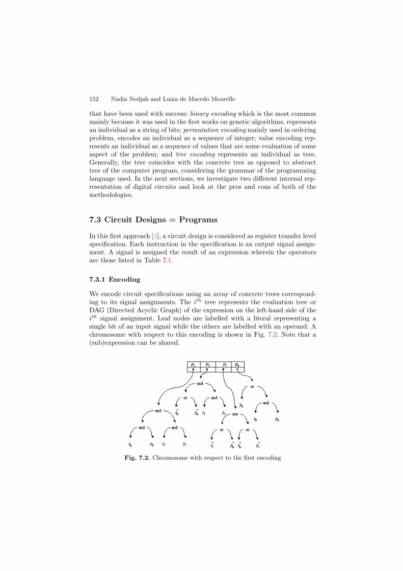
152 Nadia Nedjah and Luiza de Macedo Mourelle
that have been used with success: binary encoding which is the most commonmainly because it was used in the first works on genetic algorithms, representsan individual as a string of bits; permutation encoding mainly used in orderingproblem, encodes an individual as a sequence of integer; value encoding rep-resents an individual as a sequence of values that are some evaluation of someaspect of the problem; and tree encoding represents an individual as tree.Generally, the tree coincides with the concrete tree as opposed to abstracttree of the computer program, considering the grammar of the programminglanguage used. In the next sections, we investigate two different internal rep-resentation of digital circuits and look at the pros and cons of both of themethodologies.
7.3 Circuit Designs = Programs
In this first approach [4], a circuit design is considered as register transfer levelspecification. Each instruction in the specification is an output signal assign-ment. A signal is assigned the result of an expression wherein the operatorsare those listed in Table 7.1.
7.3.1 Encoding
We encode circuit specifications using an array of concrete trees correspond-ing to its signal assignments. The ith tree represents the evaluation tree orDAG (Directed Acyclic Graph) of the expression on the left-hand side of theith signal assignment. Leaf nodes are labelled with a literal representing asingle bit of an input signal while the others are labelled with an operand. Achromosome with respect to this encoding is shown in Fig. 7.2. Note that a(sub)expression can be shared.
Fig. 7.2. Chromosome with respect to the first encoding

7 Evolutionary Digital Circuit Design 153
7.3.2 Genetic Operators
Crossover recombines two randomly selected individuals into two fresh off-spring. It may be single-point or double-point or uniform crossover [3]. Crossoverof circuit specification is implemented using single-point and double-pointcrossovers [3] as described in Fig. 7.3 and Fig. 7.4. We also analysed theimpact of a variable double-point crossover that may degenerate into a single-point one when one of the points is 1 or coincides with the number of theexpected output signals.
(a) Before applying crossover (b) After applying crossover
Fig. 7.3. Single-point crossover of circuit specifications
The impact of each of the crossover techniques implemented is depicted inthe chart of Fig. 7.5. The data used were obtained from 100 runs of the evolu-tionary process for the same input/output behaviour. The best runs in termsof convergence are represented. Fig. 7.5 shows clearly that the evolutionaryprocess converges faster when the variable crossover is exploited. This is acrossover whose crossing points are generated randomly each time a crossoveroperation takes place.
We monitored the convergence point after 600 generations for the threecrossover techniques and computed the relative gain occasioned. The results

154 Nadia Nedjah and Luiza de Macedo Mourelle
(a) Before applying crossover (b) After applying crossover
Fig. 7.4. Double-point crossover of circuit specifications
generation
fitn
ess
single-point crossoverdouble-point crossover
variable crossover
0
50
100
150
200
250
300
0 100 200 300 400 500 600
Fig. 7.5. The impact of the crossover operator for circuit specifications

7 Evolutionary Digital Circuit Design 155
are given in Table 7.3. The speedup is relative to the single-point crossover andis computed as the ratio of the number of generations when using the single-point crossover and that when using the crossover technique in question. Theoptimisation objectives, i.e. size and time were considered of equal preferenceand so ω1 = ω2 = 0.5. From the figures given in Table 7.3, we can notice thatthe variable crossover technique is the most efficient and should be used tospeedup the evolutionary process of circuit design.
Table 7.3. Performance comparison of the specification crossover variations
Crossover Convergence point Gain
single-point 593 1.00double-point 410 1.45variable 280 2.12
One of the important and complicated operators for genetic programming[2] is the mutation. It consists of changing a gene of a selected individual. Thenumber of individuals that should suffer mutation is defined by the mutationrate while how many genes should be altered within a chosen individual isgiven by the mutation degree.
Here, a gene is the expression tree on the left hand side of a signal as-signment symbol. Altering an expression can be done in two different waysdepending the node that was randomised and so must be mutated. A noderepresents either an operand or operator. In the former case, the operand,which is a bit in the input signal, is substituted with either another inputsignal or simple expression that includes a single operator as depicted in Fig.7.6. The decision is random. In the case of mutating an operand node to anoperator node, we proceed as Fig. 7.7.
7.4 Circuit Designs = Schematics
Instead of textual specification, a circuit design can also be represented by agraphical one, which is nothing but the corresponding schematics. So in thissecond approach [5], a circuit design is considered as map of gates given inTable 7.1. The first row of gates receives the input signals while the last rowdelivers the circuit output signals.
7.4.1 Encoding
We encode circuit schematics using a matrix of cells that may be intercon-nected. A cell may or may not involved in the circuit schematics. A cell consistsof two inputs or three in the case of a mux, a logical gate and a single output.

156 Nadia Nedjah and Luiza de Macedo Mourelle
Fig. 7.6. Operand node mutation for circuit specification
Fig. 7.7. Operator node mutation for circuit specification

7 Evolutionary Digital Circuit Design 157
A cell may draw its input signals from the output signals of gates of previousrows. The gates includes in the first row draw their inputs from the circuitglobal input signal or their complements. The circuit global output signals arethe output signals of the gates in the last raw of the matrix. A chromosomewith respect to this encoding is given in Fig. 7.8.
We encode circuit schematics using a matrix of cells that may be intercon-nected. A cell may or may not be involved in the circuit schematics. A cellconsists of two inputs or three in the case of a mux, a logical gate and a singleoutput. A cell may draw its input signals from the output signals of gates ofprevious rows. The gates include in the first row draw their inputs from thecircuit global input signal or their complements. The circuit global outputsignals are the output signals of the gates in the last raw of the matrix. Achromosome with respect to this encoding is given in Table 7.4. It representsthe circuit of Fig. 7.8. Note that the input signals are numbered 0 to 3, theircorresponding negated signals are numbered 4 to 7 and the output signals arenumbered 16 to 19. If the circuit has n outputs with n < 4, then the signalsnumbered 16 to n are the actual output signals of the circuit.
Table 7.4. Chromosome for the circuit of Fig. 7.8
〈1, 0, 2, 8〉 〈5, 10, 9, 12〉 〈7, 13, 14, 11, 16〉〈2, 4, 3, 9〉 〈1, 8, 10, 13〉 〈3, 11, 12, 17〉〈3, 1, 6, 10〉 〈4, 9, 8, 14〉 〈7, 15, 14, 15, 18〉〈7, 5, 7, 7, 11〉 〈4, 10, 11, 15〉 〈1, 11, 15, 19〉
Fig. 7.8. Chromosome with respect to the second encoding

158 Nadia Nedjah and Luiza de Macedo Mourelle
7.4.2 Genetic Operators
Crossover of circuit schematics, as for specification crossover, is implementedusing four-point crossover. This is described in Fig. 7.9. The four-pointcrossover can degenerate to either the triple, double or single-point crossover.Moreover, These can be either horizontal or vertical.
1 2
1 2
3
4
3
4
×
Fig. 7.9. Four-point crossover of circuit schematics
The four-point crossover degenerates into a triple-point one whenever oneof the crossover points (say p) coincides with one of the sides of the circuitgeometry. It is a horizontal triple-point when p is one of the vertical crossoverpoints, as in Fig. 7.10–(a) and Fig. 7.10–(b) and horizontal otherwise, as inFig. 7.10–(c) and Fig. 7.10–(d).
The four-point crossover degenerates into a double-point one whenevereither both horizontal points or vertical points coincide with the low and highor left and right limits of the circuit geometry respectively. The horizontaldouble-point crossover is described in Fig. 7.11–(a) and the horizontal one inFig. 7.11–(b).
The four-point crossover can also yield a horizontal and vertical single-point crossover as described in Fig. 7.12–(a) and Fig. 7.12–(b) respectively.The vertical single-point crossover happens when the horizontal crossoverpoints coincide with the low and high limits of the circuit geometry and theone of the vertical points coincides with the left or right limit of the circuitgeometry. On the other hand, the horizontal single-point crossover happenswhen the vertical crossover points coincide with the left and right limits of

7 Evolutionary Digital Circuit Design 159
1
1
2
3
2
3
×
(a) right horizontal
1
1
2
3
2
3
×
(b) left horizontal
1 2
1 2
3
3
×
(c) top vertical
1 2
1 2
3
3
×
(d) bottom vertical
Fig. 7.10. Triple-point crossover of circuit schematics
1
2
1
2
×
(a) horizontal
1 2
1 2
×
(b) vertical
Fig. 7.11. Double-point crossover of circuit schematics

160 Nadia Nedjah and Luiza de Macedo Mourelle
1
1
×
(a) horizontal
1
1
×
(b) vertical
Fig. 7.12. Single-point crossover of circuit schematics
the circuit geometry and one of the horizontal crossover points coincide withlow or high limit of the circuit geometry.
We studied the impact of each of the four-point, triple-point, double-pointand single-point crossover. The purpose is to identify the best suited crossovertechnique, i.e. the one that allows a faster convergence to the minimal circuitdesign. The chart of Fig. 7.13 plots the average fitness function over 100 runsof the evolutionary process for the input/output behaviour that was usedin the analysis of Fig. 7.5. This was done for each type of crossover. For allcrossover techniques, except four-point crossover, we allowed variable crossingpoints. So, the triple-point crossover can be one of those depicted in Fig. 7.10,the double-point crossover can be one of those showed in Fig. 7.11 and finally,the single-point crossover can be one of those described in Fig. 7.12. The chartof Fig. 7.13 also plots the variable crossover which cab simply be one of thecrossover operators described so far for circuit schematics. In this case, thefour crossing points are generated randomly every time the operation takesplace. So, the circuit schematics can be recombined according to one of thetechniques showed in Fig. 7.9 – Fig. 7.12.
As before, we monitored the convergence point after 400 generations for thefive crossover techniques and computed the speedup occasioned. The resultsare given in Table 7.5. Recall that the speedup is relative to the single-pointcrossover and is computed as the ratio of of generation number. Furthermore,the optimisation objectives, i.e. size and time were considered of equal impor-tance. From the figures given in Table 7.5, we can establish that the variablecrossover technique is the most efficient and should be used to speedup theevolutionary process of circuit design.
The mutation operator can act on two different levels: gate mutation orroute mutation. In the first case, a cell is randomised and the correspondinggate changed. When a 2-input gate is altered by another 2-input gate, the

7 Evolutionary Digital Circuit Design 161
generation
fitn
ess
single-point crossover
double-point crossover
triple-point crossover
four-point crossover
variable crossover
⊕
⊕ ⊕ ⊕ ⊕ ⊕ ⊕⊕
⊕⊕
⊕⊕ ⊕
⊕ ⊕
⊕
⊕
⊕
⊕
⊕
⊕
⊕
⊕
⊕
⊕
⊕
⊕
⊕⊕ ⊕ ⊕
⊕ ⊕⊕ ⊕ ⊕ ⊕
⊕
⊕
⊕ ⊕ ⊕
0
50
100
150
200
250
300
0 100 200 300 400
Fig. 7.13. The impact of the crossover operator for circuit schematics
Table 7.5. Performance comparison of the schematics crossover variations
Crossover Convergence point speedup
single-point 351 1.00double-point 285 1.23triple-point 213 1.65four-point 180 1.95variable-point 93 3.77
mutation is thus completed. However, when a 2-input gate is changed to a3-input gate (i.e. to a mux), the mutation operator randomise an additionalsignal among those allowed (i.e. all the input signals, their complements andall the output signals of the cells in the rows previous). Finally, when a mux
is mutated to a 2-input gate, the selection signal is simply eliminated. Thesecond case, which consists of route mutation is quite simple. As before, a cellis randomised and one of its input signals is chosen randomly and mutatedusing another allowed signal. The mutation process is described in Fig. 7.14.
7.5 Result Comparison
In this section, we compare the evolutionary circuits yield when using the firstencoding and those evolved using the second encoding. For this purpose, weuse five examples that were first used in [1]. For each one of these examples,we provide the expected input/output behaviour of the circuit and the circuit

162 Nadia Nedjah and Luiza de Macedo Mourelle
Fig. 7.14. Mutation of circuit schematics
designs evolved by the first and the second approach. For each of the evolutionprocess, we state the number of generation for the same input parameters.
The truth table of the benchmarks is given in Table 7.6. Apart from bench-mark (a), which has only three inputs, the remaining benchmarks, i.e. (b), (c)and (d), need four inputs. On the other hand, apart from benchmark (d),which yields three output signals, the rest of the benchmarks, i.e. (a), (b) and(c) propagate a single output signal. The circuits receive input signal X andpropagate output signal Y .
The resulted circuit for the benchmark (a) using the first encoding is aregiven through the respective schematics in Fig. 7.15 as well as the correspond-ing VHDL data-flow specification in Fig. 7.16.
The circuit that was genetically programmed for the benchmark (b) (i.e.,using the first encoding) is are shown by the corresponding schematics in Fig.7.17 as well as the respective VHDL data-flow specification in Fig. 7.18.
The circuit evolved for the benchmark (c) by genetic programming is areshown by the corresponding schematics in Fig. 7.19 as well as the respectiveVHDL data-flow specification in Fig. 7.20.

7 Evolutionary Digital Circuit Design 163
Table 7.6. Truth table of the circuit used as benchmarks to compare both encodingmethodologies
X3 X2 X1 X0 Ya Yb Yc Yd2 Yd1 Yd0
0 0 0 0 0 1 1 1 0 00 0 0 1 0 1 0 0 1 00 0 1 0 0 0 1 0 1 00 0 1 1 1 1 0 0 1 00 1 0 0 0 0 1 0 0 10 1 0 1 1 0 0 1 0 00 1 1 0 1 1 1 0 1 00 1 1 1 0 1 1 0 1 01 0 0 0 - 1 1 0 0 11 0 0 1 - 0 1 0 0 11 0 1 0 - 1 1 1 0 01 0 1 1 - 0 0 0 1 01 1 0 0 - 0 0 0 0 11 1 0 1 - 1 1 0 0 11 1 1 0 - 0 1 0 0 11 1 1 1 - 0 1 1 0 0
Fig. 7.15. Encoding 1: evolved circuit for the benchmark a

164 Nadia Nedjah and Luiza de Macedo Mourelle
ENTITY C1_a IS
PORT (X: IN BIT_VECTOR(2 DOWNTO 0);
Y: OUT BIT);
END C1_a;
ARCHITECTURE Data_Flow OF C1_a IS
BEGIN
Y <= MUX(X[2], X[0] AND NOT X[2], MUX(X[0], NOT X[0], NOT X[1]));
END Data_Flow;
Fig. 7.16. Encoding 1: Data-Flow specification of the evolved circuit for the bench-mark a
Fig. 7.17. Encoding 1: evolved circuit for the benchmark b
ENTITY C1_b IS
PORT (X: IN BIT_VECTOR(2 DOWNTO 0);
Y: OUT BIT);
END C1_b;
ARCHITECTURE Data_Flow OF C1_b IS
SIGNAL T: BIT_VECTOR(1 DOWNTO 0);
BEGIN
T[0] <= NOT X[0];
T[1] <= NOT X[2];
Y <= MUX(T[0], X[1] XOR MUX(T[1], X[1], T[0]), X[0] NOR T[1]));
END Data_Flow;
Fig. 7.18. Encoding 1: Data-flow specifcation of the evolved circuit for the bench-mark b

7 Evolutionary Digital Circuit Design 165
Fig. 7.19. Encoding 1: evolved circuit for the benchmark c in Table 7.6
ENTITY C1_c IS
PORT (X: IN BIT_VECTOR(3 DOWNTO 0);
Y: OUT BIT);
END C1_c;
ARCHITECTURE Data_Flow OF C1_c IS
SIGNAL T: BIT_VECTOR(0 DOWNTO 0);
BEGIN
T[0] <= NOT X[3];
Y <= ((T[0] NAND X[2]) XNOR T[0]) OR MUX(T[0], X[1], T[0]);
END Data_Flow;
Fig. 7.20. Encoding 1: Data-flow specification of the evolved circuit for the bench-mark c
The circuit evolved for the benchmark (d) by genetic programming is areshown by the corresponding schematics in Fig. 7.21 as well as the respectiveVHDL data-flow specification in Fig. 7.22.
Once again, for benchmark (a), we obtained the circuit whsoe schematicsare given in Fig. 7.23 and the respective VHDL data-flow specification areshown in Fig. 7.24. This was done using the genetic algorithms (i.e., the secondencoding).
The circuit evolved for the benchmark (b) GA (first encoding) is shown bythe corresponding schematics in Fig. 7.25 as well as the equivalent data-flowspecification in Fig. 7.26.
The circuit evolved for the benchmark (c) by genetic algorithm is are shownby the corresponding schematics in Fig. 7.27 as well as the respective VHDLdata-flow specification in Fig. 7.28.

166 Nadia Nedjah and Luiza de Macedo Mourelle
Fig. 7.21. Encoding 1: evolved circuit for the benchmark d
ENTITY C1_d IS
PORT (X: IN BIT_VECTOR(2 DOWNTO 0);
Y: OUT BIT_VECTOR(2 DOWNTO 0));
END C1_d;
ARCHITECTURE Data_Flow OF C1_d IS
SIGNAL T: BIT_VECTOR(3 DOWNTO 0);
BEGIN
T[0] <= NOT X[3];
T[1] <= T[0] NAND X[2];
T[2] <= NOT X[2] AND X[0];
T[3] <= T[0] XNOR X[1];
Y[0] <= T[0] NOR (T[1] OR T[2]);
Y[1] <= MUX(T[1], T[0], T[2]);
Y[2] <= MUX(T[1], X[3], T[3]);
END Data_Flow;
Fig. 7.22. Encoding 1: Data-flow specification of the evolved circuit for the bench-mark d
The circuit evolved for the benchmark (d) by genetic algorithm is areshown by the corresponding schematics in Fig. 7.29 as well as the respectiveVHDL data-flow specification in Fig. 7.29.
In Table 7.7, we provide the characteristics of the circuits evolved, whichare the size in terms of gate-equivalent and the signal propagation delay in sec-onds. We also present the average numbers of generations that were necessaryto reach the shown result. These numbers of generations were obtained for 100different evolutions. In the last column of Table 7.7, we compute the average

7 Evolutionary Digital Circuit Design 167
Fig. 7.23. Encoding 2: evolved circuit for the benchmark a in Table 7.6
ENTITY C2_a IS
PORT (X: IN BIT_VECTOR(2 DOWNTO 0);
Y: OUT BIT);
END C2_a;
ARCHITECTURE Data_Flow OF C2_a IS
BEGIN
Y <= MUX(X[0] AND X[1], X[0] XOR X[1], X[2]);
END Data_Flow;
Fig. 7.24. Encoding 2: Data-flow specification of the evolved circuit for the bench-mark a
Fig. 7.25. Encoding 2: evolved circuit for the benchmark b in Table 7.6
speedup. Note that for both encodings, we exploited the variable crossovertechnique.
The graphical representation of the fitness values of the evolved circuitswhen using both encoding is depicted in Fig. 7.31 while that of the perfor-mance factor is given in Fig. 7.32. The numerical data are listed in Table 7.8.The hardware area and response time are considered to be of equal impor-tance. The performance factor is computed as in (7.2) and the speedup isobtained using (7.3) which is simply the Amadahl’s law.

168 Nadia Nedjah and Luiza de Macedo Mourelle
ENTITY C2_b IS
PORT (X: IN BIT_VECTOR(2 DOWNTO 0);
Y: OUT BIT);
END C2_b;
ARCHITECTURE Data_Flow OF C2_b IS
SIGNAL T: BIT_VECTOR0 DOWNTO 0);
BEGIN
T[0] <= NOT X[0];
Y <= (NOT MUX(T[0], X[2], MUX(T[0], X[1], X[2])) XOR X[2]) XOR X[1];
END Data_Flow;
Fig. 7.26. Encoding 2: Data-flow specification of the evolved circuit for the bench-mark b
Fig. 7.27. Encoding 2: evolved circuit for the benchmark c in Table 7.6
ENTITY C2_c IS
PORT (X: IN BIT_VECTOR(3 DOWNTO 0);
Y: OUT BIT);
END C2_c;
ARCHITECTURE Data_Flow OF C2_c IS
BEGIN
Y <= (X[3] XNOR X[1]) OR MUX(X[0] XNOR X[3], X[1], X[2]);
END Data_Flow;
Fig. 7.28. Encoding 2: Data-flow specification of the evolved circuit for the bench-mark c
performance =100 × fitness
#generations(7.2)
speedup =performance2
performance1(7.3)

7 Evolutionary Digital Circuit Design 169
Fig. 7.29. Encoding 2: evolved circuit for the benchmark d in Table 7.6
ENTITY C2_d IS
PORT (X: IN BIT_VECTOR(2 DOWNTO 0);
Y: OUT BIT);
END C2_d;
ARCHITECTURE Data_Flow OF C2_a IS
SIGNAL T: BIT_VECTOR(1 DOWNTO 0);
BEGIN
T[0] <= NOT X[2] NOR X[0];
T[1] <= NOT X[0] NOR X[3];
Y[0] <= (X[1] XNOR X[2]) AND (X[1] XOR X[3]);
Y[1] <= T[0] OR ((T[1] NOR X[3]) AND X[1]);
Y[2] <= T[1] OR (X[2] AND (T[0] NOR X[3]));
END Data_Flow;
Fig. 7.30. Encoding 2: Data-flow specification of the evolved circuit for the bench-mark d
Table 7.7. Number of gate-equivalent and generations required to evolve the circuitspresented
Benchmark Size1 Size2 Size3 Time1 Time2 #Gen1 #Gen2
(a) 11 8 12 0.4865 0.424 302 29(b) 14 15 20 0.6985 0.973 915 72(c) 12 9 20 0.6205 0.639 989 102(d) 20 22 34 0.7015 0.888 1267 275

170 Nadia Nedjah and Luiza de Macedo Mourelle
Table 7.8. Performance comparison of the impact of the studied encodings
Benchmark Fitness1 Fitness2 Performance1 Performance21 speedup
(a) 5.743 4.212 1.902 14.53 7.64(b) 7.349 7.986 0.803 11.09 13.81(c) 6.310 4.819 0.638 4.725 7.41(d) 10.35 11.44 0.817 4.161 5.09
Fig. 7.31. Fitness comparison
Fig. 7.32. Performance Comparison

7 Evolutionary Digital Circuit Design 171
7.6 Conclusion
In this chapter, we described two different encoding to be used in digitalcircuit evolution. In the first representation, we view a circuit design as a pro-gram that provide its specification. The second representation, in contrast,views a circuit as schematics that graphically describe the composition of thecircuit. For each one of these encoding, we presented the variations of ap-plicable genetic operators. We evaluated the impact of these variations onthe convergence of the evolutionary design process. From the experiences per-formed with different crossover techniques, we can conclude that the variablecrossover technique allows maintain a better diversity within the generationalpopulation and so yields an earlier convergence. Furthermore, we comparedthe performance of two genetic algorithms that use the described encoding.The comparison was peformed using 4 different benchmarks that were firstused in [1]. The evolution process was repeated 100 times for each one of thebenchmarks and the average number of generation that was required to reacha valid solution was recorded. In general, the evolved circuits are of the samecomplexity in terms of size and times. However, the number of generationnecessary to reach a valid solution when using the first encoding was almost10 times bigger. We computed the speedup according to Amadahl’s law. Thiswas about 8.5 in favour of the second encoding. The size of a solution de-signed by human using classical simplification methods is also presented. Theevolved solutions are always better compared the ones classically designed.
References
1. Coelho, A.A.C., Christiansen, A.D. and Aguirre, A.H., Towards Automated Evo-lutionary Design of Combinational Circuits, Comput. Electr. Eng., 27, pp. 1–28,(2001) 161, 171
2. Koza, J. R., Genetic Programming. MIT Press, (1992) 1553. Miller, J.F., Thompson, P. and Fogarty, T.C., Designing Electronics Circuits
Using Evolutionary Algorithms. Arithmetic Circuits: A Case Study, In GeneticAlgorithms and Evolution Strategies in Engineering and Computer Science,Quagliarella et al. (eds.), Wiley Publisher (1997) 153
4. Nedjah, N. and Mourelle, L.M., Evolvable Hardware Using Genetic Programming,Proc. 4th International Conference Intelligent Data Engineering and AutomatedLearning - IDEAL 2003, Hong Kong, China, Lecture Notes in Computer Science,Vol. 2690, Springer-Verlag, (2003) 152
5. Poli, R. Efficient evolution of parallel binary multipliers and continuous symbolicregression expressions with sub-machine code GP, Technical Report CSRP-9819,University of Birmingham, School of Computer Science, December (1998) 155
6. Rhyne, V.T., Fundamentals of digital systems design, F.F. Kuo (Ed.) Prentice-Hall Electrical Engineering Series, (1973) 149
7. Thompson, A., Layzel, P. and Zebelum, R.S., Explorations in design space: un-conventional design through artificial evolution, IEEE Transactions on Evolu-tionary Computations, 3(3):81–85, (1996) 147, 148

8
Evolving Complex Robotic BehaviorsUsing Genetic Programming
Michael Botros
Department of Electrical Communication and Electronics,Cairo University, Giza, Egypt.
Genetic programming (GP) applies the evolution model to computer pro-grams. It searches for the best fit computer program through the use of bi-ologically inspired operators such as reproduction, crossover and mutation.It has proven to be a powerful tool for automatically generating computerprograms for problems that are too complex or time consuming to be pro-grammed by hand. Example of these problems is writing control programs forautonomous robots to achieve non trivial tasks.
In this chapter, a survey of different methods for evolving complex roboticbehaviors is presented. The methods represent two different approaches. Thefirst approach introduces hierarchy into GP by using library of procedures ornew primitive functions. The second approach use GP to evolve the buildingmodules of robot controller hierarchy. Comments including practical issuesof evolution as well as comparison between the two approaches are also pre-sented.
The two approaches are presented through a group of experiments. Allexperiments used one or more Khepera robots which is a miniature mobilerobot widely used in the experiments of evolutionary robotics.
8.1 Introducing Khepera Robot
Khepera is a miniature mobile robot that is widely used in laboratories anduniversities in conducting experiments aiming at developing new control algo-rithms for autonomous robots. It was developed by the Swiss Federal Instituteof Technology and manufactured by K-team [1] [2]. Khepera robot is cylin-drical in shape with a diameter of 55 mm and a height of 30 mm. Its weightis about 70 gm. Its small size and weight made it ideal robotic platform forexperiments of control algorithms that could be carried out in small environ-ments such as a desktop.
M. Botros: Evolving Complex Robotic Behaviors Using Genetic Programming, Studies in Com-putational Intelligence (SCI) 13, 173–191 (2006)www.springerlink.com c© Springer-Verlag Berlin Heidelberg 2006

174 Michael Botros
The robot is supported by two wheels; each wheel is controlled by a DCmotor that can rotate in both directions. The variation of the velocities of thetwo wheels, magnitude and direction, will result in wide variety of resultingtrajectories. For example if the two wheels rotate with equal speeds and insame direction, the robot will move in straight line, but if the two velocitiesare equal in magnitude but different in direction the robot will rotate aroundits axis.
Fig. 8.1. Miniature mobile robot Khepera (with permission of K-team)
The robot is equipped with eight infrared sensors. Six of the sensors aredistributed on the front side of the robot while the other two are placed on itsback. The exact position of the sensors is shown in Fig. 8.2. The same sensorhardware can act as both ambient light intensity sensor and proximity sensor.
0
12 3
4
7 6
5
Fig. 8.2. The position of the eight sensors on the robot (with permission of K-team)
Each of the eight sensors consists of emitter and receiver parts so thatthese sensors can function as proximity sensors or ambient light sensors. Tofunction as proximity sensors, it emits light and receive the reflected lightintensity. The measured value is the difference between the received light in-tensity and the ambient light. This reading has range [0, 1023] and it gives

8 Evolving Complex Robotic Behaviors Using GP 175
a rough estimate how far the obstacles are. The higher reflected light inten-sity the closer obstacles are. It should be noted that we cannot find a directmapping between the sensor reading and the distance from the obstacle, asthis reading depends on factors other than the distance to the obstacle suchas the color of the obstacle.
To function as ambient light sensors, sensors use only receiver part of thedevice to measure the ambient light intensity and return a value that falls inthe range of [0, 1023]. Again, these measurements depend very strongly onmany factors such as the distance to the light source and its direction.
An interesting feature of the Khepera robot is its autonomy, which includesautonomy of power and control algorithm. For the purpose of power autonomy,the robot is equipped with rechargeable batteries that can last for about 45minutes. For experiments that may require much longer time, the robot canbe connected to a host computer by a lightweight cable to provide it with theneeded electrical power. This is an important feature that allowed long controlexperiments (such as developing evolutionary algorithms) to be carried outwithout repetitive recharging.
On the other hand, for the control autonomy, the robot’s CPU board isequipped with MC68331 microcontroller with 512K bytes of ROM (systemmemory) and 256K bytes of RAM (user memory). This RAM memory canaccommodate reasonable length program codes to provide control autonomy.The robot can be programmed using Cross-C compiler and the program willbe uploaded to the robot through serial port communication with a hostcomputer. Also the robot can be remotely controlled by a host computerwhere the control commands are sent to the robot through the serial linkconnection mentioned above. This mode of operation has an advantage ofusing computational power of the host computer.
8.2 Evolving Complex Behaviorsby Introducing Hierarchy to GP
In this section, we will present how complex behaviors can be evolved by in-troducing hierarchy to genetic programming. Two different approaches willbe presented. The first approach builds a subroutine library in GP. The sub-routines in the library will be available to individual programs as an aug-mentation to the function set. The second approach uses function set that ismore suitable to the nature of the input sensory information. The functionset that will be presented here consists of neural networks. Each of the twodifferent approaches will be presented along with an experiment that appliedthis approach to evolve a complex robotic behavior.

176 Michael Botros
8.2.1 Genetic Programming with Subroutine Library
Providing a program solution to artificial intelligence problems (such as theproblem of controlling a robot) usually includes building functions or proce-dures to do common calculations. They also discover the common similaritiesin the problem to be solved. The overall solution to the problem has the hi-erarchy of a main program that invoke a number of functions, which may inturn call other lower level functions. However, this program hierarchy is notavailable in the programs evolved using genetic programming. They consist oftrees that make use of primitive functions without providing a technique toevolve procedures or functions along with the main program. Fig. 8.3 shows atypical program tree. The buildings units of this tree are the set of terminalsT and the set of primitive functions F given by:
T = t1, .., tmF = f1, .., fn
To overcome this problem in genetic programming, Koza in [3] [4] and[5] suggested a method for automatically detecting functions and subroutinesand representing them inside the same tree of individual programs. In thiscase the program tree would consist of usual branches that form the programand return results, and a number of branches (l) each defining one functionof the automatically defined functions ADFs. These ADF branches are notexecuted unless called by one of the value returning branches. Fig. 8.3 showsan example of program tree with ADF branches.
a - Program tree in GP
root
f1
t1 f2
t3t2
Branchthat
returnsresult
b - Program tree in GP implemnting ADF
root
ADF1
InputList ofADF1
ConventionalGP branchDefinition
of ADF1
Fig. 8.3. Example of program tree in conventional GP and GP implementing ADF
The function set available to each individual is extended to include any ofthe l branches defining ADFs within the same individual tree. F in this caseis given as follows:

8 Evolving Complex Robotic Behaviors Using GP 177
F = f1, .., fn, ADF1, .., ADFl
But the ADF in a program subtree can not be used in another individualwithin the same generation, Furthermore, if an effective ADF is found asbranch in a less fit individual, it will have small chance of reproduction andpropagation to the next generations. These reasons led to thinking of a methodto save well performing ADF functions in a subroutine library. In [6], Hondoet al. suggested a method for building that library and updating it accordingto fitness criteria. The function set in this case will be extended to includeall the subroutines available in the library beside the ADFs represented asbranches in the program tree as before. F in this case is given as follows:
F = f1, .., fn, ADF1, .., ADFl, SR1, .., SRL
where SRi in this case is the subroutine number i in the library whose size isL.
The choice of a certain subroutine to be placed in the library dependson how well it performed when called by individual programs in the currentgeneration. One possible fitness measure would be given by [6]:
fitness SRi=
∑Ci
j=1 fj
Ci
where Ci is the number of individual programs that called subroutine SRi
and fj is the fitness of each of these programs. By using fitness measures forsubroutines, library is kept updated with effective subroutines at the expenseof more computations.
The rest of this section will present a robotic experiment, by K. Yanai et al.[7], that maintained the subroutine library in the GP to evolve three roboticcontrollers for a team of three Khepera robots to simulate the escape behaviorfrom a room during emergency time. The task set to these robots requiresthat they leave the room through an exit (marked with a color different fromthe color of the rest of the wall). To use this exit the robots have to pressthree buttons (given as black objects) in the room. This mission should becompleted with a given limit of time. All the three robots are equipped withcameras to recognize different colors; however, each robot is allowed to movewith a different speed. So the team in this case consists of similar robots butwith different capabilities.
The genetic programming process used a different sub-population for eachrobot in the team. Individuals in each sub-population implemented ADFbranches in addition to access to subroutine library in order to evolve hi-erarchical programs. The evolution process of each robot is not indepen-dent on the other two robots. Two aspects of interactions exist betweenthe sub-populations. First, fitness evaluation of an individual from a givensub-population will take place while the best individuals in the other two

178 Michael Botros
sub-populations are used as controlling programs for the other two robots.Second, migration is performed among the three sub-populations to allow theexchange of possible individuals with high fitness.
The evolution process took place in simulated environments. Different sim-ulated environments were used throughout the generations to evaluate thefitness of the individuals. Fig. 8.4 shows a possible example of these envi-ronments. The fitness functions used was the same for each individual in thethree sub-populations. The fitness function, as seen in the next expression,encouraged early pushing of the three buttons (third term) and early leavingof the room (fourth term). The fitness function is given by [7]:
fitness = C1 + C2 + bonus for pushing all buttons early+ bonus for leaving early (8.1)
where C1 is a constant added to the fitness for each robot robot that pushesa button and C2 is a variable that is inversely proportional to the distancebetween each robot and the exit at the end of fitness evaluation.
Fig. 8.4. Environment of the experiment
The evolution process lasted for 30 generations and the best fit individualswere tested in simulated as well as real environments. Evidence of coordinationbetween robots was observed during these tests. Typical behavior of best fitindividual in the environment can be described as follows: the fast robots rushto push the closest buttons, while the robot with the slowest speed would godirectly to the exit since it can not afford to navigate the room searching for

8 Evolving Complex Robotic Behaviors Using GP 179
the buttons. The rest of the team would press any remaining buttons andthen head to the exit [7].
This experiment showed possibility of evolving controlling programs thatpossess hierarchy similar to the hand-coded programs. This experiment andother robotics experiments applying hierarchical GP takes this approach onestep higher by proving its validity in a more complex domain of problems.The next section will discuss another approach that utilizes neural networksas elements of the function sets.
8.2.2 Neural Networks and the Control of Mobile Robots
In the this section and the next one a method for combing the neural networkswith genetic programming will be presented. The primitive function set wasbuilt using neural networks to detect different situations faced by the robot.This section will give a brief review of artificial neural networks (ANN) basicsthat will be useful for the reader who is unfamiliar with ANN for betterunderstanding of next section.
Single neuron model: ANN consists of interconnection of processing unitscalled neurons which is inspired by the biological neurons of the nervous sys-tem. In the biological neuron, it receives all inputs stimuli in the form ofspiking electrical activity and these inputs are large enough they can activatethe neuron so that it will in turn send electrical signals to other neurons con-nected to it. In our ANN model, the neuron receives the inputs x1, ..., xn andsum them after being weighted by corresponding weights w1, ..., wn (calledsynaptic weights) and if the result is above a threshold b then the net resultcan generate an output y through a nonlinear function Φ. The following equa-tion describes the input-output relation of a class of artificial neurons. Thissingle neuron model is usually represented graphically as shown in Fig. 8.5.
y = φ(n∑
i=1
wixi − b)
x1
x2
xn
wn
w1
y
Single Neuron
Fig. 8.5. Model of a single neuron

180 Michael Botros
Interconnecting neurons: A widely used class of neural network architec-ture is obtained by arranging neurons in cascaded layers as shown in Fig. 8.6.Each layer consists of an array of neurons whose outputs are connected to thenext layer inputs. The first layer inputs are the ANN inputs and the last layeroutputs are the ANN outputs. Fig. 8.6 shows ANN with three layers: inputlayer, hidden layer, and output layer.
.
.
Input 1 ..
Input 2
Input n
Output 1
Output 2
Three Layers ANN
Fig. 8.6. Artificial neural network with three layers
Learning: Now we have an ANN with given architecture, how can it per-form a given function or how can it give a desired output for a given input? Theanswer of this question is through the learning process of the neural networkwhich includes adjusting the synaptic weights w’s and threshold b of each neu-ron such that the overall ANN will give the desired output for a given input.A widely used, though not the only one, algorithm for learning the weightsand thresholds is through back propagation. In this algorithm, pairs of inputsand corresponding desired outputs are used to learn the weights iteratively. Ineach iteration, the inputs are applied to the ANN and the error between theactual and desired output is used to update the weights in way to minimizethe squared error. We can look at this type of learning as an adaptive algo-rithm or optimization problem in which the weights are optimized iterativelyto minimize an objective function that depends on the error.
Why ANN is useful to robotics: The ability to lean by example is a desirablefeature in neural networks that can benefit robotics. Examples of input sensoryinformation and corresponding robot output (such as robot velocity in case ofmobile robots) can be used to train neural networks to be employed as roboticcontroller. Another desirable feature is the highly nonlinear relation betweenthe ANN inputs and outputs due to the nonlinear function φ of each neuron.This nonlinear relation is useful when we want to have an output with some

8 Evolving Complex Robotic Behaviors Using GP 181
degree of insensitivity to inputs corrupted with noise such as robot sensoryinputs.
Evolutionary algorithms and neural networks: Genetic Algorithm GA canbe incorporated with ANN in different ways. One way is to use the evolutionprocess of the genetic algorithm to search for the optimal set of weights andthresholds. Example of this approach applied to robotics can be found in [9],in which GA acted as a optimization tool for the weights of a neural networkcontroller. Another way is let the GA evolve the architecture of the ANNalong with its weights. Example of this method applied to robotic applicationcan be found in [10]. The next section discusses further incorporation betweenthe genetic programming and ANN.
In this section, a brief introduction to ANN concepts was presented. Theinterested reader can find detailed treatment of ANN in dedicated textbookssuch as [11].
8.2.3 Using Neural Networks as Elements of the Function Set
If we want to write a program to identify possible situations faced by therobot, it may be difficult to identify these situations using logic expressions inthe sensors. For example, if we want to identify the situation in which thereis an obstacle in front of the robot, a possible logic expression can be (sum offront sensors > numerical threshold). Given the noisy nature of real sensors,this expression may not be triggered in every time there is an obstacle in frontof the sensors. Noise or distance to obstacle may cause the sensors values to beactive but less than the given threshold. For the case of Khepera robot, andother robots utilizing infrared sensors, the proximity sensor readings dependson the color of the obstacle too as we mentioned earlier in the first section.One potential solution to this problem is using a neural network whose inputcomes from the proximity sensors (and possibly from ambient light sensorstoo to cover the cases of different obstacles with different colors) and whoseoutput is used to identify these situations. The synaptic weights will need tobe trained first using example situations to be identified. The remaining partof this section will present an experiment that used trained neural networksas primitive function in the genetic programming process.
The experiment is performed by K. Lee et al. [12]. The task of the robotis to reach a target location which is marked by the presence of a light sourceand at same time robot has to avoid the obstacles present in its environment.To reach its target, it will need the ambient light sensors I0,.., I7 to detectthe light source and it will use the proximity sensors S0,.., S7 to avoid theobstacles.
During the robot path to the target it will encounter situations when theobstacles are in front of it or to its left or right. Also, avoiding obstacles maychange its orientation with respect to the target so it will need to detect suchsituations (target to left, right, .., etc). The above described situation werechosen to be the function set of the GP while the terminal set was the basic

182 Michael Botros
action that can be taken by the robot such as moving forward, or backwardand turning left or right. Typical code example would consist of a tree ofelements of the function and terminal set such as the one depicted in Fig. 8.3part (a) and as shown in figure 1 in [12].
Each of these situation described above was build as a function of theeight proximity sensors and eight ambient light sensors. These functions wereimplemented as a neural network that consisted of 16 input neurons and oneoutput neuron in a fashion similar to the general layered architecture shownin Fig. 8.6. The synaptic weights were trained by back propagation. In backpropagation the weights are adjusted iteratively to give the desired output.The error between the current and desired output is used to tune the weightsas discussed in the previous section. Now, having trained the weights of theneural networks to detect the situations that can face the robot, they areready to act as function set.
The genetic programming process took place in simulation. Different sim-ulated environments were used for fitness evaluation. They contained arrange-ments of obstacles and two light sources. The robots will be rewarded for eachtime they reach any of light sources and would be punished for colliding withany obstacle. The fitness function used is given by [12]:
fitness = C1Ncollision
Nsteps+
Nsteps − C2Nreaching target
Nsteps(8.2)
where Nsteps is the number of the steps the individual program is allowedto perform in each fitness evaluation, Ncollisions is the numbers of the collisionsthat occurred during these steps and Nreachingtarget is the number of successfulachieving of the task by approaching the light sources. The two constants C1
and C2 constitute a tradeoff between the importance of the avoiding obstaclesand approaching the target.
After 100 generations, the results of the experiments showed the decrease ofthe average fitness and increase of the number of reaching the target with theincrease of the number of generations. The best fit individual was transformedto a real robot and was tested in a real environment with obstacles and singlelight source. The robot was able to find its way between the obstacles to reachthe light source in the corner of the room [12].
8.2.4 Comments
Two methods for including hierarchy inside the GP have been presented. Firstmethod evolve the main program along with the procedures and maintain aprocedure library while the second method uses a new function set consistingof neural networks. In this section, we will discuss some of practical points inboth methods.
• Reducing human designer early choices in evolution process. Inthe first method and in conventional GP too, human designer has to choose

8 Evolving Complex Robotic Behaviors Using GP 183
a set of primitive functions, their parameters, and write their code. On theother hand, the second method offers a more automated method for thesechoices. The learning process of neural network will tune the synapticweights of the network to perform the right task by choosing the rightsensors. For example, in the previous experiment neural networks wereused to detect two sets of situations, the first set is related to the obstacle(obstacle to the left, to the right ... etc) and the other related to the tar-get (target ahead, target to the left .. etc). After training, we expect thatthe weights associated with proximity sensors are higher than those corre-sponding to light sensors in the first set and less effective in determiningthe output of the network in the second set.
• Moving from simulation to real robots. Very few evolution exper-iments are carried on real robots in real environments. The common ap-proach is evolving the controller in simulation and then testing the best fitindividual using a real robot and real environment. This approach avoidslengthy experiment time and hardware problems if real robots were used.However, a drawback of this approach is difference between the robot be-havior in simulated and real environments which may arise due to thenoise present in real sensors which have not been accounted for in thesimulation.The hand coded primitive functions of first experiment had to be mod-ified after transition from simulation to real worlds. For example in thefirst experiment of the robot team escape, function sets that detect col-ors were used (buttons and exit were differentiated based on their colors).These functions have to be edited to account for the difference betweenthe simulated camera and the real camera [7]. In the second experimenttoo, the neurons threshold values had to be modified when testing the bestfit individual on real robot [12]. However this step was necessary becausethe learning of the neural network was based on samples of the simulatedsensor values. We believe that this modification could have been avoidedif the learning process used samples of the real sensor data.
• Size of the evolved programs. First method of using hierarchicalGP is associated with increasing the number of branches to implementADF. Some methods were proposed to control the growth of the code [8].For example, segments of code that will not be reached and will not beexecuted, called introns, can be discovered and removed. If I is a logicalcondition, then if the tree contains the expression ( If true or I), I will beinfective intron. GP can detect such introns by associating a counter withelements of terminal sets and functions and incrementing it each time theyare evaluated. The expression whose all terminals and functions counterswere not incremented could be a possible intron. Upon detecting an intron,GP can edit it to become effective or delete it to control the tree growth.

184 Michael Botros
8.3 Evolving Complex Behaviorsby Introducing Hierarchy to the Controller
In this section we will present two examples of evolving complex robotic be-haviors by using GP to evolve the building modules of a hierarchical robotcontroller. The concept of using hierarchy in robot controllers is similar toconcept of “divide and conquer” in software design and programming and italso follows the main design steps which are:
Step one: The complex behavior is broken down into simpler behaviors ortasks.
Step two: A program or controller is designed to implement this behavior.Step three: A method is used for coordination or arbitration between different
behaviors.
Using different methods to carry out steps one and three results in differentarchitectures of controllers [13]. In the next subsections we will present twomain architectures: subsumption architecture and action selection architecturewhich will both be used in the two examples that will come next.
8.3.1 Subsumption Architecture
In subsumption architecture [13], step one is carried by assigning each oneof the simpler behaviors to one of the layers of the architecture with higherpriority behaviors placed in upper layers. The sensory information is input toall layers, also outputs of the lower layers may be used as inputs to higherlayers. For coordinating between the outputs of different layers, a fixed prioritysystem is used which is predefined by the designer of the controller. The higherlayers output has higher priority to propagate to the physical output of thecontroller such as the robot motor speeds. It can also inhibit or pass the outputof lower layers to the controller output as shown in Fig. 8.7.
A simple example of subsumption architecture is a controller to enable therobot to explore its environment while avoiding the obstacles. This behaviorcould be divided into to basic behaviors: exploring the environment and avoid-ing the obstacle while the last one given higher priority to avoid damagingthe robot or hurting humans in the environment.
SensorReadings
Lower level behavior
Upper layer behavior
Inhibitor
Controlleroutput
Fig. 8.7. Subsumption architecture

8 Evolving Complex Robotic Behaviors Using GP 185
An apparent advantage of this architecture is simplicity in arbitratingbetween behaviors. Also, the behavior of the robot is expected to be dominatedby the upper layer behaviors so we are able to predict the robot behavior indifferent environment. However some tasks may require the robot to switchbetween behaviors dynamically according to the current situation, for examplesearching for a specific object, then carrying it to a given target. In this casethe first behavior (searching) should be dominant for sometime and then therobot needs to switch to the second behavior (carrying object) when the objectis found. In this class of tasks, an architecture that handles dynamic priorities,such as action selection architecture, is needed.
8.3.2 Action Selection Architecture
Beahvior 2 Beahvior 3Beahvior 1
Action selection
Sesnsor Readings
Controller output
Fig. 8.8. Action selection architecture
In action selection [17], step one is done by breaking the complex behaviorinto simpler behaviors and associating with each of them an activation levelwhich reflects its current importance and suitability to the situation. The ac-tivation level is function of the current robot’s goal and its sensory readings.Step three is carried as follows: before each action taken by the robot, thatoutput of each simple behavior module is evaluated as well as its activationlevel. The behavior with the highest activation level is allowed to propagateits output to the controller output. Since these activation levels are dynami-cally changing, action selection belongs to the class of architectures that usedynamic priorities.
Fig. 8.8 shows an example of action selection control architecture in whichthree behaviors compete, through their activation levels, to gain control overthe robot. It should be noted that it is possible to have a tree-like structurewithin the action selection controller as shown in Fig. 8.8. In this case boththe left and the right behaviors are further broken into even simpler behaviors.We will encounter another example of this tree-like architecture in one of theexperiments presented after this subsection.

186 Michael Botros
Action selection 0
Action selection 1 Action selection 2
Behavior 1-bBehavior 1-a Behavior 2-a Behavior 2-b
Fig. 8.9. Action selection architecture with tree-like structure
Having introduced these two architectures, we are now ready to move tothe next section to see how GP can be used within each architecture to evolveits constituting modules.
8.3.3 Using GP to Evolve Modules of Subsumption Architecture
In this experiment, performed by S. Kamio et al. in [16], genetic program-ming is used to evolve the modules of a robot controller with a subsumptionarchitecture. The controller is intended to act as central controller for a robotteam consisting of two Khepera robots with different capabilities described asfollows:
1. Robot 1 is a Khepera robot provided with a camera mounted on the topof the robot.
2. Robot 2 is a Khepera robot provided with a gripper module that is alsomounted on the top of the robot. The gripper can perform two main ac-tions: picking and releasing the object. The robot can detect the presenceof an object in the gripper by using a light barrier sensor placed insidethe gripper. Fig. 8.10 shows the robot while using the gripper to hold anobject.
The task of the controller is to construct coordination between the robotsso that the second robot, which is equipped with the gripper only without anyvision capabilities, will locate objects found in the experiment environmentand carry them to a certain goal area (marked by its different color). Clearlythis would require a help from the first robot with the camera that would beused to estimate the distance between itself and the object (dobject) and thesecond robot (drobot2) [16].
To achieve the previously described task, the central controller was de-signed using subsumption architectures, in which each subtask (or behavior)is assigned to one layer of the architecture with the higher layers able toprocess the outputs of lower layers and to decide whether to inhibit or pass itto the final outputs. These layers are described as follows [16]:

8 Evolving Complex Robotic Behaviors Using GP 187
Fig. 8.10. Khepera robot with the gripper mounted on the top of it (with permissionof K-team)
1. Lower layers: They are responsible for signal processing of camera signalsand estimating drobot2 and dobject.
2. Intermediate layer: The task of this layer is to generate the motor speedsof the two robots based on the distance estimate from the previous layer.
GP was used to evolve this module. Beside the inputs from the previouslevel, the terminal set included basic actions for the two robots such asmoving forward and rotation to left and right. Generations consisted of2000 individuals each. Each individual was tested in a number of simulatedenvironments where this module was allowed to control the two robots fora number of steps till robot 2, with the gripper, has moved a distanceequals twice the its initial distance to the object. After being tested indifferent environments, the fitness of the individual was evaluated as themaximum, over all testing environments, of the final distance between theobject and the robot with gripper. After the end of one evaluation genera-tion, the individuals of the new generation would then be produced by thecrossover and mutation operator. The results of best evolved individualfor this module will be presented after discussing the last layer.
3. Higher layer: The task of this layer is to decide when robot 2 would openits gripper to hold the object and when to release it. This layer was pro-grammed by human programmers.

188 Michael Botros
When the best fit individuals after the evolution process, the two robotsshowed the desired guided navigation behavior. Robot 1, with the camera,starts moving first acting like the explorer followed with robot 2. Comparedto individuals of first generations, individuals in last generations showed moredirect pathes to the object and to the goal area [16].
This experiment was example of using GP to evolve the modules of con-troller architecture. A question may rise here asking if it could be possibleto evolve a program for the entire controller directly in a single GP processinstead of evolving each module. This could be a possible approach, howeverin this case the genetic programming will search a larger space of programsthat achieve the overall task rather than the smaller space of each module.It may seem that this single GP will save effort by designing only one fitnessfunction and running the GP once, however it may need larger number ofgenerations for convergence.
8.3.4 Using GP to Evolve Modulesof Action Selection Architecture
In this experiment, performed by W. Lee et al. in [18], GP is utilized toevolve a robotic controller with action selection architecture. The task of thecontroller is to enable to robot to navigate in the environment to locate acylindrical object and push it towards a target marked by its light source.Proximity sensors of the robot will help it locate the object while the ambientlight sensors will help it locate the light source.
The complex task mentioned above can be decomposed using action selec-tion architecture. At any time, the main controller will act as an arbitrationor action selection module that arbitrates between two basic behaviors: (1)navigation in the environment and (2) pushing the object. The later can befurther implemented as another action selection module that arbitrates be-tween two sub-behaviors: (2-a) pushing the box forward and (2-b) rotatingaround the object, which will be useful when the object slips from the ro-bot and it needs to adjust itself to a suitable pushing position relative to theobject. This architecture can be implemented as a tree as shown in Fig. 8.9.
All the behaviors and action selection modules were evolved using GP. Wewill start first by the GP process of behavior modules then the action selectionmodules.
The behavior modules were represented as logic building blocks. The pro-gram will be built up using “And” and “Or” functions and comparators thatcompare the input sensor values with numerical constants. So the function setconsisted of these comparators beside the logic gates while the terminal setconsisted of the input sensors and the numerical constants [18].
The fitness function of behavior module was designed on the sensor levelto encourage the individuals to acquire the desired behavior. For example,the behavior (2-a) of pushing the object forward encouraged high front sensorvalues so that the robot would maintain the object in its front direction.
8 Evolving Complex Robotic Behaviors Using GP 189
The action selection modules are program units that select which behaviorsto be executed. It can be thought of as a program that can output either “1”or “0” depending on the behavior selected, so by this way they can be builtup using logic components as the behavior modules so the function set againconsisted of logic gates. Since the selection of the suitable behavior will dependon the current situation which need to estimated using the robot sensors, theterminal set need to contain the include the input sensors. The readings ofthe input sensors will be compared with numerical constants to produce “1”or “0” results suitable to be used with the logic building blocks.
Evolution of each module was carried in simulated environments thentested in real environments. The overall controller, built using best fit in-dividuals of each module, enabled the robot to navigate in the environmenttill finding the object, and then it switches to the other behavior of pushingthe object [18].
8.4 Comments
Two different approaches for evolving complex behaviors were discussed. Thefirst one introduces the hierarchy to the GP by allowing it to evolve func-tions along with the main program. The second one uses the hierarchy of thecontroller to evolve the building modules of the controller architecture.
• Evolved program hierarchy. In the first approach the hierarchy is au-tomatically generated by the GP through the use of ADFs while in theother approach, the hierarchy is enforced by the initial design. Also eachmodule is responsible for certain part of the overall behavior. However wecan not assert that each ADF in the first approach corresponds to a sim-ple behavior. However, it can be interesting idea to study the existence ofrelation between some of the automatically defined functions, especiallythose which have acquired high fitness or used by many individuals, andsome of the simple tasks performed by the robot. This can be achievedby observing the robot behavior during the execution of segments of theprogram tree that call these ADFs.
• The GP design. The first approach uses a single GP process to evolveboth the main program and the its functions, while in the second approachwe have a number of evolution processes equal to the number of the be-havior modules plus the number or arbitrator modules (whether it usesaction selection or other behavior coordination methods).The fitness function in the first approach usually reflects the overall desiredgoals of the controller. This can be seen in equations (8.1) and (8.2). Onthe other hand, fitness functions in the other approach take some effort tobe designed on the low level suitable for simple behavior required by eachmodule.

190 Michael Botros
Also having a special GP process for each module makes it possible tospecify different terminal and function sets suitable for each module. Ter-minal set will contain only the sensor inputs needed by this module whichcan be less than all the available number of sensory inputs, thus allowingthe search in a smaller space.
• Reusability. In the second approach, we have a different evolved pro-gram for each module thus allowing the reusability of these modules. Onthe other hand, the automatically defined functions of the first approachare branches within the main program tree, which are less suitable forreusing compared with the second approach.
• Using both approaches jointly. In this case, the human designer per-forms logical decomposing of the complex robot behavior and suggests ahierarchy for the controller. The modules of this architecture are allowedto be implemented by programs that use subroutines and functions. TheGP will be used to explore this lower level hierarchy search for best fitprogram with its subroutines.
8.5 Summary
In this chapter, two possible approaches for evolving complex behaviors werediscussed. In the first approach, the GP is used to explore possible hierarchy inthe solution through implementing ADF and maintaining a subroutine libraryor using neural networks as primitive functions.
In the second approach, human programmer set the architecture of therobot controller and then the GP is used to evolve each module of this archi-tecture. Two examples of architectures were discussed, the subsumption archi-tecture and action selection architecture. Two experiments were presented todemonstrate this approach. The first used subsumption architecture to controla team of two robots with different capabilities to implement a cooperativebehavior. The second experiment used action selection architecture to allowswitching between the simpler behaviors that constitute the main behavior.
Acknowledgement
The author would like to thank S. Mary, S. Mina, S. Kirolos, S. George, andS. Mercorious for their support.

8 Evolving Complex Robotic Behaviors Using GP 191
References
1. K-Team (1999) Khepera User Manual,” Lasuanne, Switzerland 1732. Mondada F, Franz F, Paolo I (1993) Mobile Robot Miniaturisation: A Tool
for Investigation in Control Algorithm. Proceedings of the Third InternationalSymposium on Experimental Robotics, Kyoto, Japan 173
3. Koza J (1992) Hierarchical Automatic Function Definition in Genetic Program-ming. Proceedings of Workshop on the Foundations of Genetic Algorithms andClassifier Systems 297–318, Morgan Kaufmann Publishers Inc., Vail Colorado,USA 176
4. Koza J (1993) Simultaneous Discovery of Detectors and a Way of Using theDetectors via Genetic Programming. IEEE International Conference on NeuralNetworks 3:1794–1801, San Francisco, NJ, USA 176
5. Koza J (1993) Simultaneous Discovery of Reusable Detectors and SubroutinesUsing Genetic Programming. Proceedings of the 5th International Conferenceon Genetic Algorithms ICGA:295–302, Morgan Kaufmann Publishers Inc. 176
6. Hondo N, Iba H, Kakazu Y (1996) Sharing and Refinement for Reusable Subrou-tines of Genetic Programming. Proceedings of IEEE International Conferenceon Evolutionary Computation ICEC: 565–570 177
7. Yanai K, Iba H (2001) Multi-agent Robot Learning by Means of GeneticProgramming: Solving an Escape Problem. Proceedings of the 4th Interna-tional Conference on Evolvable Systems: From Biology to Hardware: 192–203,Springer-Verlag 177, 178, 179, 183
8. Iba H, Terao M (2000) Controlling effecective Introns for Multi-Agent Learningby Genetic Programming. Proceedings of Genetic and Evolutionary ConferenceGECCO: 419–426 183
9. Floreano D, Mondada F (1996) Evolution of Homing Navigation in a Real Mo-bile Robot. IEEE Transactions on Systems, Man, and Cybernetics (B) 2:396–407 181
10. Hulse M, Lara B, Pasemann F, Steinmetz U (2001) Evolving Neural BehaviourControl for Autonomous Robots. Max-Planck Institute for Mathematics in theSciences, Leipzig, Germany 181
11. Haykin S (1999), Neural Networks: a Comprehensive Foundation, Second edi-tion, Prentice Hall, Upper Saddle River, NJ 181
12. Lee K, Byoung-Tak Z (2000) Learning Robot Behaviors by Evolving GeneticPrograms. 26th Annual Confjerence of the IEEE Industrial Electronics Society,IECON 2000 4:2867–2872 181, 182, 183
13. Brooks R (1986) A Robust Layered Control System For Mobile Robots. IEEERobotics and Automation 2:14–23 184
14. Arkin R (1998) Behavior-Based Robotics. The MIT press, Cambridge, USA15. Koza J (1993) Evolution of Subsumption Using Genetic Programming. In: F.
Varela and P. Bourgine (eds) Toward a Practice of Autonomous Systems 110–119, Cambridge, MIT Press, USA
16. Kamio S, Hongwei L, Mitsuhasi H, Iba H (2003) Researches on Ingeniously Be-having Agents. Proceedings of NASA/DoD Conference on Evolvable Hardware208–217 186, 188
17. Maes P (1989) The Dynamics of Action Selection. Proceedings of the EleventhInternational Joint Conference on Articial Intelligence IJCAI89 2:991–998 185
18. Lee W, Hallam J, Lund H (1997) Learning Complex Robot Behaviours by Evo-lutionary Approaches. 6th European Workshop on Learning Robots EWLR642–51 188, 189

9
Automatic Synthesis of MicrocontrollerAssembly Code Through Linear GeneticProgramming
Douglas Mota Dias1, Marco Aurelio C. Pacheco1 and Jose F. M. Amaral2
1 ICA — Applied Computational Intelligence LabElectrical Engineering DepartmentPontifıcia Universidade Catolica do Rio de JaneiroR. Marques de Sao Vicente 225, Gavea, Rio de Janeiro, CEP 22453-900, RJBrazil(douglasm,marco)@ele.puc-rio.br
2 Department of Electronics EngineeringUERJ — Rio de Janeiro State UniversityR. Sao Francisco Xavier, 524, Maracana,Rio de Janeiro, CEP 20550-013, [email protected]
This chapter considers the application of linear genetic programming in theautomatic synthesis of microcontroller assembly language programs that im-plement strategies for time-optimal or sub-optimal control of the system tobe controlled, based on mathematical modeling through dynamic equations.One of the difficulties presented by the conventional design of optimal controlsystems lies in the fact that solutions to problems of this type normally in-volve a highly non-linear function of the system’s state variables. As a result,it is often not possible to find an exact mathematical solution. As for the im-plementation of the controller, there arises the difficulty of programming themicrocontroller manually in order to execute the desired control. The researchthat has been done in the area of automatic synthesis of assembly languageprograms for microcontrollers through genetic programming is surveyed inthis chapter and a novel methodology in which assembly language programsare automatically synthesized, based on mathematical modeling through dy-namic plant equations, is introduced. The methodology is evaluated in twocase studies: the cart-centering problem and the inverted pendulum problem.The control performance of the synthesized programs is compared with that ofthe systems obtained by means of a tree-based genetic programming method.The synthesized programs proved to perform at least as well, but they had
D. M. Dias et al.: Automatic Synthesis of Microcontroller Assembly Code Through LinearGenetic Programming, Studies in Computational Intelligence (SCI) 13, 193–227 (2006)www.springerlink.com c© Springer-Verlag Berlin Heidelberg 2006

194 Douglas M. Dias et al.
the additional advantage of supplying the solution already in the final formatof the implementation platform selected: a microcontroller.
9.1 Introduction
Automatic control has played a vital role in the advancement of engineeringand science. In addition to being a major asset in the area of space vehicles,missile guiding systems, robotic and other similar systems, automatic controlhas become an important and integral part of modern industrial and man-ufacturing processes. For example, automatic control is an essential elementin the numerical control machine tools used in the manufacturing industries,in the design of automatic pilot systems used in the aerospace industry andin the automobile and truck projects of the automobile industry. It is alsoessential in industrial operations, as in the case of pressure, temperature, hu-midity, viscosity and flow control in the process industries. The theoretical andpractical advancement of automatic control provides means by which optimalperformances from dynamic systems may be obtained, by which productivitymay be improved, by which the tiresome job of carrying out many repetitiveroutine operations manually may become less burdensome, and much more[21].
The types of difficulties encountered in the course of developing a controlsystem may be divided according to two stages: design and implementation.
At the designing stage, the problem arises during the mathematical devel-opment of a solution to the control problem. Although many physical relationsare often represented by linear equations, in most cases the relations are notexactly linear. In fact, a meticulous study regarding physical systems revealsthat even the so-called ”linear systems” are really linear only within limitedoperating ranges. In practice, many electromechanical, hydraulic, pneumatic,etc. systems involve nonlinear relations between the variables. For example,the output of a component may saturate for large input signals. Non-linearitiesof the quadratic rule type may occur in some of the components. Some impor-tant control systems are nonlinear regardless of the input signal values. Forinstance, in ”on-off” control systems, the control action is either ”on” or ”off”and there is no linear relation between the controller’s input and its output[21].
Analytical methods for solving nonlinear systems that are higher than thefourth order do not exist. Due to this mathematical difficulty, it normallybecomes necessary to introduce ”equivalent” linear systems as substitutes forthe nonlinear ones. These equivalent linear systems are valid only within alimited operating range. Only after a nonlinear system has been approximatedby a linear mathematical model can analytical tools be applied for analysisand design purposes [21].
In practice, proportional integral derivative PID controllers are used. PIDcontrollers are useful on account of their general applicability to most control

9 Automatic Synthesis of Microcontroller Assembly Code Through LGP 195
systems. In the field of continuous process control systems, it is known for afact that PID and modified PID control structures have proved to be usefulby providing satisfactory control. However, these controllers are unable toprovide optimal control in a number of specific situations [21].
Solutions to optimal control problems normally involve a higher-order non-linear function of the system’s state variables. As a result, it is often notpossible to find an exact mathematical solution to optimal control problems.
As for the implementation stage, there arises the problem of developing aprogram which, when executed by a digital system, is able to perform the con-trol strategy that has been determined in the previous stage. The fact is thatusing computers or microcontrollers (MCs) to implement controllers resultsin considerable advantages. Many of the difficulties encountered with analogimplementation may be avoided. For example, there are no problems withregard to precision or component alterations. It is easier to have sophisticatedcalculations in the control law and to include logical and nonlinear functions.
In the so-called embedded systems, where MCs are widely used, it is some-what difficult to program the MC by comparison to a conventional computerbecause the computational power of an MC’s central processing unit (CPU)is much more limited on account of its small instruction set and the littlememory space available.
9.2 Survey on Genetic Programming Appliedto Synthesis of Assembly
A number of papers on genetic programming applied to the synthesis of as-sembly language programs have been presented lately. Table 9.1 shows a tax-onomy that includes some of the main studies on the evolution of assemblylanguage programs.
9.2.1 JB Language
One of the earliest approaches to evolution of computer programs similar tomachine code is the JB language [9]. Cramer formulated his method as ageneral approach to evolve programs, but his register machine language is inmany ways similar to a simple machine code language and will thus serve asa good illustration for register machine GP. He uses a string of digits as thegenome. Three consecutives digits represent an instruction. The first integerin the triple determines the type of instruction. This is similar to the syntaxof a machine code instruction which has specific bit fields to determine thetype of instruction. There are five different instructions or statements in JB.INCREMENT adds one to a specified register. The register number is givenby the second digit of the triple. ZERO clears a register while SET assigns avalue to a register. There are also BLOCK and LOOP instructions that groupinstructions together and enable while-do loops. JB employs a variable-length

196 Douglas M. Dias et al.
Table 9.1. Taxonomy over the evolution of assembly language programs
System Author Description Refs.
JBLanguage
N.L.Cramer,TexasInstruments
• Variable-size linear chromosomeearlier, in tree later
• One of the earliest approaches
[9]
VRM-M L.Huelsbergen,Bell Labs.
• Fixed-size linear chromosome• Objective was to evolve loops.
[12]
AIMGP P.Nordin,Universityof Dortmund
• Fixed-size linear chromosome earlier,variable size, later
• Ran only on SUN SPARC platformearlier, also on Intel x86, later
[18][19]
GEMS R.L.Crepeau,NCCOSCRDTE
• Fixed-size linear chromosome• Evolution of a ”Hello world” program
for the Z-80 CPU
[10]
string crossover. In part to avoid infinite loops, Cramer later abandoned thismethod in favor of an approach using a tree-based genome [5].
9.2.2 VRM-M
Huelsbergen has used a formal approach to evolve code for a virtual reg-ister machine (VRM) [12]. His goal was to evolve an iterative multiplica-tion program from lower level instructions such as JUMP, COMPARE, ADD,DECREMENT and others. Execution loops are formed spontaneously fromthese primitives given fitness cases and a maximum number of allowed execu-tion steps. The evolutionary algorithm also uses a linear representation of theprograms (string of instructions) and a linear crossover operator exchangingsubstrings. His system is implemented in the functional formal language Stan-dard Meta Language (SML). GP results are compared favorably with resultsusing random search.
9.2.3 AIMGP
Nordin has used the lowest level binary machine code as the programs in thepopulation [18][19]. Each individual is a piece of machine code that is calledand manipulated by the genetic operators. There is no intermediate languageor interpreting part of the program. The machine code program segmentsare invoked with a standard C function call. The system performs repeatedtype cast between pointers to arrays for individual manipulation and pointersto functions for the execution of the programs and evaluation of individuals’fitness. Legal and valid C-functions are put together, at run time, directlyin memory by the genetic algorithm. This system was formally known as
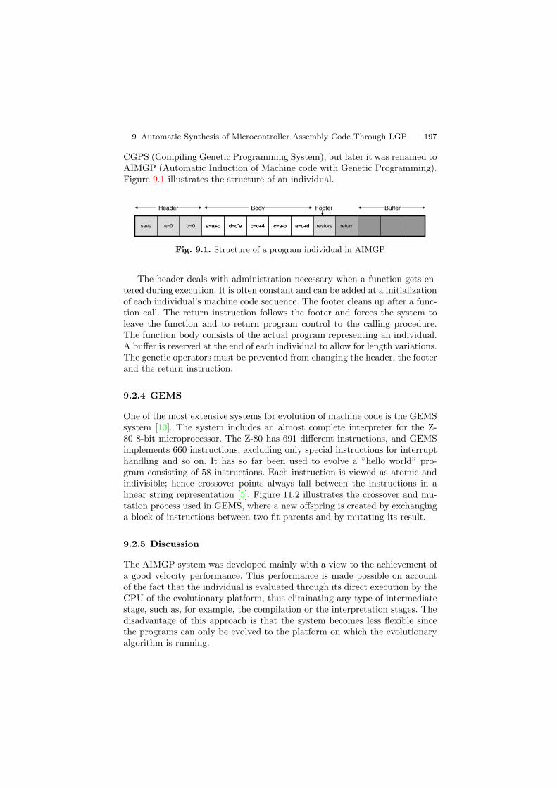
9 Automatic Synthesis of Microcontroller Assembly Code Through LGP 197
CGPS (Compiling Genetic Programming System), but later it was renamed toAIMGP (Automatic Induction of Machine code with Genetic Programming).Figure 9.1 illustrates the structure of an individual.
returnrestorea=c+dc=a-bc=c+4d=c*aa=a+bb=0a=0save returnrestorea=c+dc=a-bc=c+4d=c*aa=a+bb=0a=0save
Header Body Footer Buffer
Fig. 9.1. Structure of a program individual in AIMGP
The header deals with administration necessary when a function gets en-tered during execution. It is often constant and can be added at a initializationof each individual’s machine code sequence. The footer cleans up after a func-tion call. The return instruction follows the footer and forces the system toleave the function and to return program control to the calling procedure.The function body consists of the actual program representing an individual.A buffer is reserved at the end of each individual to allow for length variations.The genetic operators must be prevented from changing the header, the footerand the return instruction.
9.2.4 GEMS
One of the most extensive systems for evolution of machine code is the GEMSsystem [10]. The system includes an almost complete interpreter for the Z-80 8-bit microprocessor. The Z-80 has 691 different instructions, and GEMSimplements 660 instructions, excluding only special instructions for interrupthandling and so on. It has so far been used to evolve a ”hello world” pro-gram consisting of 58 instructions. Each instruction is viewed as atomic andindivisible; hence crossover points always fall between the instructions in alinear string representation [5]. Figure 11.2 illustrates the crossover and mu-tation process used in GEMS, where a new offspring is created by exchanginga block of instructions between two fit parents and by mutating its result.
9.2.5 Discussion
The AIMGP system was developed mainly with a view to the achievement ofa good velocity performance. This performance is made possible on accountof the fact that the individual is evaluated through its direct execution by theCPU of the evolutionary platform, thus eliminating any type of intermediatestage, such as, for example, the compilation or the interpretation stages. Thedisadvantage of this approach is that the system becomes less flexible sincethe programs can only be evolved to the platform on which the evolutionaryalgorithm is running.

198 Douglas M. Dias et al.
...
BIT 3,D
OR B
POP IY
LD SP
...
...
BIT 3,D
OR B
POP IY
LD SP
...
...
POP A
DEC A
INC C
SRA D
...
...
POP A
DEC A
INC C
SRA D
...
...
BIT 3,D
DEC A
INC C
LD SP
...
...
BIT 3,D
DEC A
INC C
LD SP
...
...
SLA E
DEC A
INC C
LD SP
...
...
SLA E
DEC A
INC C
LD SP
...
...
BIT 3,D
OR B
POP IY
LD SP
...
...
BIT 3,D
OR B
POP IY
LD SP
...
...
SLA E
DEC A
INC C
LD SP
...
...
SLA E
DEC A
INC C
LD SP
...
Most fit parent
Least fit parent
Crossover
Mutation
Deleted from population
Retained population individual
New population individual
Fig. 9.2. The GEMS crossover and mutation process
The remaining systems mentioned above, however, did not aim to excelin evolutionary velocity, but rather in offering the possibility of evolving pro-grams to a specific type of assembly language. The system presented in thischapter also belongs to this category because its purpose was the creationof programs for an existing PIC microcontroller. This approach is somewhatsimilar to that of the GEMS system since the GEMS also evolves programsfor an existing device, which, in its case, is a Z80 CPU.
In the same manner as the AIMGP system, the system that has beendeveloped in this paper made use of a variable-size linear chromosome. Thismakes it possible to try to optimize the code of the evolved programs.
9.3 Design with Microcontrollers
9.3.1 Microcontrollers
As integrated circuits (ICs) became cheaper and microprocessors (MPs) beganto emerge, the simpler MPs began to be used in the implementation of dedi-cated tasks, such as printer control, velocity adjustment, step motor control,elevator controls, etc.
However, implementing a control system involved assembling very largecircuits and this often represented a price increase. The cost of such applica-tions depended on the price of the MP and of the peripherals (ROM and RAMmemories, ports, A/D and D/A converters, etc.), as well as on the number ofconnections and the circuit board size.

9 Automatic Synthesis of Microcontroller Assembly Code Through LGP 199
For the purpose of reducing the price, the idea of placing these peripheralsand the CPU within a single IC was conceived. This would not only reduce theprice and the size of the printed circuit, but would also increase the system’scredibility. Moreover, it is not necessary for a control-dedicated CPU to bevery fast, nor does it need to have such an extensive and powerful instructionset. Instructions are not necessary in work involving floating points, strings,or vectors. The addressing mechanisms must also be simple. In other words,it is possible to simplify the CPU. And that is how microcontrollers came onthe scene - they are simple, cheap and efficient.
9.3.2 Time-Optimal Control
Control-related problem-solving is a task that involves conducting the stateof a system from a given initial state to a specific final state. The state ofthe system is described by a set of state variables. The transition from onestate to a next one is obtained by means of a control variables set. Thus,the control problem consists of selecting the values of these variables so asto cause the system to move towards the specified final state. The goal of anoptimal control is to perform control at an optimal cost, where cost can bemeasured in terms of time, fuel, energy or some other type of measurement.What is important in a minimum-time problem class is to transfer the stateof a system to a specific final state as quickly as possible [4].
Solutions to control and optimal control problems normally involve ahigher-order nonlinear function of the system’s state variables. As a conse-quence, many times it is not possible to find an exact mathematical solutionto control problems. Moreover, in the case of practical problems, it often hap-pens that the mathematical model of the system itself is not available and itmay become necessary to obtain the control based on a set of data that havebeen obtained empirically.
It is also important to point out that although many of the physical re-lations in the system that is to be controlled are often represented by linearequations, in most cases the real relations are not exactly linear [21].
As already said, the use of computers for the implementation of controllerspresents considerable advantages [3]. There are, however, certain types of sys-tems in which it is not possible to make use of computers. They are the so-called embedded systems, where MCs are widely employed. MCs also presentthe advantage of providing computational resources for the control systemthat is to be implemented, though in a much more limited manner. It canbe said that genetic programming has much to contribute in this scenario. Ifon the one hand, it represents a means by which to automatically synthesizeprograms that implement control and optimal control strategies, even in thecase of problems where it is not possible to obtain a mathematical solution,on the other, it is able to do so specifically for a platform that has limitedcomputational resources, as in the case of the MC.

200 Douglas M. Dias et al.
9.4 Microcontroller Platform
This section contains a brief presentation of the PIC18F452 Microchip [16], an8-bit RISC microcontroller, with a simple architecture, largely employed andthat has been adopted as a platform in the automatic synthesis of assemblycode.
The architecture of this MC is of the Harvard type, in other words, thereare two internal buses, one containing data, the other, instructions. The pro-gram and the data therefore occupy different memories. The program memoryis of the flash type with storage capacity of 32 Kbytes, that is, 16,384 16-bitinstructions.
The data RAM is responsible for the storage of the file registers and ofthe special registers. The area of this memory, which is related to the general-purpose registers, stores the variables defined by the programmer which are tobe written and read by the program. In turn, the area related to the registersfor special use can be read and written by both the program and the hardwaresince the MC makes use of these registers for executing the program and forprocessing the Arithmetic-Logic Unit (ALU). These are the registers thatcontain, for example, the status flags. This memory has a storage capacity of1,536 bytes.
The ”W” accumulator is an 8-bit register that directly stores the ALUoperation results and it is also addressable.
There is a hardware multiplier in the ALU (8 x 8 multiply), which bringswith it the advantages of a better computational throughput and a reductionin the size of the necessary code in multiplication algorithms. Multiplicationis carried out, without any signal, between two 8-bit registers and their 16-bitresult is stored in two specific 8-bit registers: ”PRODH” and ”PRODL”.
In addition, there are 5 input/output ports (I/O ports), where port ”A”has 7 bits, ports ”B”, ”C”, and ”D” have 8 bits each and port ”E”, 3 bits. Allthese bits can be configured individually as input or output pins by means ofthe correct configurations of their respective special registers. The ports areaddressable in the data bus.
This MC has a set of 75 instructions, 22 of which were selected for theexperiments contained in this work and are indicated in table 9.2. Operand ”f”assigns the data memory register that the instruction is to use, while operand”d” assigns the destination of the result of this operation. If ”d” is zero, thenthe result will be stored in ”W”, and if it is one, in the register assigned by”f”.
These operations were chosen because the control problems discussed inthis paper make it necessary to basically deal with arithmetical and condi-tional operations. The selection of a subset of operations that is suited to thenature of the problem is indispensable as an initial stage if GP is expected toyield a good performance.

9 Automatic Synthesis of Microcontroller Assembly Code Through LGP 201
Table 9.2. Instruction subset of the PIC18F452
Mnemonic and Operands Description
ADDWF f, d Add W and fADDWFC f, d Add W and the Carry bit to fCLRF f Assigns value zero to fCPFSEQ f Compares f with W, skips next instruction if f = WCPFSGT f Compares f with W, skips next instruction if f >WCPFSLT f Compares f with W, skips next instruction if f <WDECF f, d Decrements fDECFSZ f, d Decrements f, skips next instruction if f = 0INCF f, d Increments fMOVF f, d Copies the content of fMOVFF fs, fd Copies the content of fs in fd
MOVWF f Copies the content of W in fMULWF f Multiplies W with fNEGF f Negates f (two’s complement)RLCF f, d Rotates f to the left through the Carry bitRLNCF f, d Rotates f to the left without the Carry bitRRCF f, d Rotates f to the right through the Carry bitRRNCF f, d Rotates f to the right without the Carry bitSETF f Assigns value one to all the bits of fSUBWF f, d Subtracts W from fBTFSC f, b Tests bit b of f, skips next instruction if b = 0BTFSS f, b Tests bit b of f, skips next instruction if b = 1
9.5 Linear Genetic Programming
The emergence of GP in the scientific community arose with the use of thetree-based representation, in particular with the use of LISP language in thework of Koza [14]. However, GP systems manipulating linear structures exist[7], which have shown experimental performances equivalent to Tree GP.
In linear genetic programming, the programs are represented by a linearstring of instructions, of variable size. When compared with traditional GP,which is based on tree structures, its main characteristic is that programs areevolved in an imperative language such as C [7] and machine code [18], andnot in expressions of a functional programming language, such as LISP [14].It is for this reason that this type of GP is the best option, since assemblylanguage is also an imperative language.
The implementation of the linear GP proposed in [7], for example, repre-sents an individual program as a variable-size list of instructions in C whichoperate with indexed or constant variables. In linear GP, all the operations,such as, for example, a = b+1, implicitly include an assignment to a variable.After the program is executed, the output values are stored in the assignedvariables, differently from the tree-based GP, where the assignments and mul-

202 Douglas M. Dias et al.
tiple outputs must be explicitly incorporated through the use of an extraindexed memory and of special functions for a manipulation of this type.
9.5.1 Evolution of Assembly Language Programs
Assembly language programming is frequently used when there is a need forvery efficient solutions, as is the case of applications that are strongly re-stricted in terms of run time and memory use. In general, the reasons forevolving assembly language as opposed to high-level languages are similar tothe reasons for the use of manual programming in assembly language throughthe use of mnemonics or in machine code.
This is the level at which the most efficient optimization is obtained. Itis the lowest level to which a program can be optimized, and it is also whereit is possible to obtain the highest gains. Optimization may occur as a resultof velocity, space, or both. Small individuals may be promoted by meansof a penalty for length, which is commonly known as parsimony pressure[19]. Similarly, this pressure may be applied considering the run time of theinstructions.
It is usually considered difficult to learn, program and master assembly lan-guage. Sometimes it may be easier to let the computer evolve small programsin assembly language than to learn to master the technique of programmingat this level. This is acceptable, not only in case a high-level compiler is notavailable, but also when the use of assembly language is preferred for one ofthe two above mentioned reasons.
9.6 System for Automatic Synthesisof Microcontroller Assembly
This section describes a System for Automatic Synthesis of a MicrocontrollerAssembly that makes it possible to evaluate the proposed genetic approachthrough benchmark case studies. The system also includes a simulator of theplant to be controlled and a simulator of the microcontroller.
The main routine controls the system by continuously evaluating the gener-ated assembly programs, which are executed using both plant and MC simula-tors together, and then submitted to the genetic operators in the evolutionarykernel.
Figure 9.3 shows the block diagram of the system, and the operation ofeach module is detailed in the subsequent subsections.
9.6.1 Evolutionary Kernel
This module is responsible for the evolution of the programs themselves andtherefore implements the selection and evolutionary algorithms as well as the

9 Automatic Synthesis of Microcontroller Assembly Code Through LGP 203
Evolutionarykernel
Evolutionarykernel
PlantSimulator
PlantSimulator
MCSimulator
MCSimulator
A/Dconverter
A/Dconverter
D/Aconverter
D/Aconverter
MainroutineMain
routine
Fig. 9.3. Block diagram of the system
genetic operators. The module operates by creating the initial population,selecting individuals and applying the genetic operators to these individu-als. The next subsections contain a detailed description of how this moduleoperates.
Representation of the Individuals
Given the fact that the objective of this system is to evolve programs inassembly language, it was decided that these programs would be representedby linear chromosomes [19], where each gene represents an instruction that iscomposed of the operation and of one or two operands.
In practice, this chromosome was implemented by a vector, whose lengthwas equivalent to the length of the program, with an instruction format struc-ture.
The individuals are created at the stage in which the population is ini-tialized, which is the first stage of the GP, and makes use of a process thatis similar to the one employed in [19]. First, an individual is created throughthe random selection of a length between the minimum initial length andthe maximum initial length parameters. Next, all its genes are filled in withrandomly generated instructions based on the syntax defined for assemblylanguage. This process is repeated for all the individuals of the population.
Crossover
Linear crossover consists of an exchange of code segments between two parents,according to the graphic demonstration in Figure 9.4.
A random string of instructions is selected in each parent. In Figure 11.4,the selected instructions are highlighted in gray. These sequences are ex-changed between the two parents and as a result, the descendent individualsare generated.
For the length of these individuals, the heuristic used in [6], which demon-strates by means of experiments that unrestricted exchanging of subprograms

204 Douglas M. Dias et al.
INCF R,F
INCF R,FRRCF Y,FINCF Y,W
INCF Y,WRLNCF Y,FCPFSEQ RRRCF Y,F
NEGF RCPFSEQ RRLNCF Y,FRLNCF Y,F
MOVF U,WRLNCF Y,FBTFSC Y,7swapNEGF R
ADDWFC R,WBTFSC Y,7ADDWFC R,WMOVF U,W
ADDWFC U,FINCF Y,WADDWFC U,FINCF Y,W
Offspring 2Offspring 1Parent 2Parent 1
INCF R,F
INCF R,FRRCF Y,FINCF Y,W
INCF Y,WRLNCF Y,FCPFSEQ RRRCF Y,F
NEGF RCPFSEQ RRLNCF Y,FRLNCF Y,F
MOVF U,WRLNCF Y,FBTFSC Y,7swapNEGF R
ADDWFC R,WBTFSC Y,7ADDWFC R,WMOVF U,W
ADDWFC U,FINCF Y,WADDWFC U,FINCF Y,W
Offspring 2Offspring 1Parent 2Parent 1
Fig. 9.4. Crossover of two individuals
is not advisable, was adopted. The fact is that when large program segmentsare exchanged, the crossover becomes too destructive in evolutionary terms.The approach that was suggested and adopted consisted of limiting the max-imum size of these segments and after this work was analyzed, a maximumvalue of 4 instructions was adopted.
Mutation
Mutation acts upon only one individual at a time. After crossover occurs, eachoffspring is submitted to the mutation that has a lower level of probabilitythan the crossover. The crossover and mutation probabilities are the executionparameters of a GP.
When an individual is selected for mutation, the mutation operator ini-tially selects one of the individual’s instructions and changes its content. Thetype of change is selected in a random fashion and may consist of changingthe operation or one of the two operands. This approach was also obtainedfrom [6], where it is called ”micromutation” and its purpose is to smoothenthe effect of this operator during evolution. Figure 9.5 illustrates how thisoperator works and shows the parent with examples of two possible offspring:the one on the left would be the result of a random choice in favor of changingthe operation and the one on the right, of changing the first operand.
An alternative approach to this mutation for linear GP may be the so-called ”macromutation” [6], where a randomly selected gene is simply removedor a new randomly created gene is inserted in a random position. Anotherpossible approach consists of exchanging a code segment for an entirely new,randomly selected one [5]. But the experiment results obtained in the lin-ear GP-related literature demonstrate that micromutation is more efficientbecause it is not as destructive as the others.

9 Automatic Synthesis of Microcontroller Assembly Code Through LGP 205
MULWF X
SUBWF X, W
INCF U, F
BTFSC X, 7
SETF U
BTFSC V, 7
NEGF X
MULWF X
SUBWF X, W
INCF U, F
BTFSC X, 7
SETF U
BTFSC V, 7
NEGF X
MULWF X
SUBWF X, W
ADDWF U, F
BTFSC X, 7
SETF U
BTFSC V, 7
NEGF X
MULWF X
SUBWF X, W
ADDWF U, F
BTFSC X, 7
SETF U
BTFSC V, 7
NEGF X
MULWF X
SUBWF X, W
INCF X, F
BTFSC X, 7
SETF U
BTFSC V, 7
NEGF X
MULWF X
SUBWF X, W
INCF X, F
BTFSC X, 7
SETF U
BTFSC V, 7
NEGF X
Ramdomly selectedgene
Parent
Offspring Offspring
Fig. 9.5. Mutation on an individual
Selection
This system has adopted the tournament selection genetic algorithm [19].Tournament selection is not based on a competition among all the individualsof a generation, but rather among the individuals of a subset of the population.In this type of tournament, the number of individuals, which defines the sizeof the tournament, is selected at random before a selective competition begins.The objective in this case is to allow the characteristics of the best individualsto replace those of the worst individuals. In the smallest tournament possible,two individuals compete with each other and the best one of these two isreproduced and may undergo mutation. The result of the breeding is returnedto the population and replaces the tournament loser.
The size of the tournament makes it possible for researchers to adjustselection pressure. Small tournaments cause low selection pressure, while largeones cause high pressure. Based on the system developed in [19], a tournamentsize equal to four was selected.
Tournament selection has become quite popular as a selection methodmainly because it does not require centralized fitness comparisons among allthe individuals. This not only significantly accelerates evolution, but also pro-vides a simple way of making the algorithm become parallel. With fitness-proportional selection, the communication overhead between evaluations maybe even higher [5].
Evolution
The evolutionary algorithm selected was the so-called steady-state algorithm,which is based on the tournament selection model. It should be pointed outthat the steady-state algorithm used in GP is different from the one used
206 Douglas M. Dias et al.
in genetic algorithms. In this approach, there are no fixed intervals betweengenerations. Instead, there is a continuous flow of individuals that meet, mateand breed. The offspring replace individuals that exist in the same population.This method is easy to implement and presents certain advantages with re-spect to efficiency and to possible expansion through parallelism. Good resultsfor convergence in general have been reported and the method is becomingincreasingly popular within the research community. The evolutionary algo-rithm that was specifically developed for the evolutionary kernel of the systemdiscussed in this paper is described below:
1. Four individuals from the population are randomly selected.2. The four individuals are grouped in two pairs. For each pair, the two
individuals are evaluated and their resulting fitness are compared withone another.
3. The two winners, one from each pair, are probabilistically submitted tomutation and crossover.
4. The two losers, one from each pair, are replaced by the offsprings of thetwo winners.
5. Steps 1 to 4 are repeated until the maximum number of cycles is achieved.
This is called the steady state approach because the genetic operatorsare applied asynchronously and there is no centralized mechanism for explicitgenerations. However, steady state GP results are usually presented in termsof generations. Actually, the steady state generations are the intervals thatoccur during evolution which, one might say, correspond to the generations ina generation-based GP. These intervals are computed each time that fitnessis evaluated by the same number of individuals that the generation-based GPpopulation would have. [13] contains experiments and detailed references withrespect to generation-based GP versus steady state GP.
9.6.2 Plant Simulator
Two simulators were developed, one for each case study. Each simulator wasimplemented by means of a function that takes the state variables, throughreference, and the value of the control variable. At each specific time interval,the values of the plant’s state variables are changed as a result of the controlvariable. The plant’s control variable, in turn, represents the control actionitself and results from the execution, by the MC simulator, of the programthat is being evaluated.
The kernel of this function contains the dynamic equations that mathe-matically model the physical system that is being simulated.
9.6.3 Microcontroller Simulator
This simulator was implemented by means of a function that takes the valuesof the plant’s state variables and returns the new value of the control variable.

9 Automatic Synthesis of Microcontroller Assembly Code Through LGP 207
That is, at the end of each plant simulation time interval, the program thatis being evaluated receives the updated state variable values originating fromthe plant simulator, is executed from beginning to end, and the value of thevariable that performs the control action at that given instant is returned.
As has been mentioned in section 9.3, out of the 75 instructions containedin the PIC18F452, only those pertaining to the scope of the case studies wereimplemented and the result was a total of 22 instructions.
9.6.4 A/D and D/A Converters
These converters are responsible for establishing an interface between the ana-log magnitude values with which the plant simulator works and their digitalequivalents used by the MC simulator.
A/D converters are functions that convert the analog values of the plant’sstate variables, originating from the plant simulator, to their respective digitalvalues, which are supplied to the MC simulator. In other words, these modulessimulate the operation of physical A/D converters, which convert the analogmagnitude values obtained by their respective sensors to their equivalent dig-ital values, which are furnished to the MC.
In turn, the D/A converter is a function that converts the digital valueof the control variable, originating from the MC simulator, to its respectiveanalog value, which is supplied to the plant simulator. Hence, this modulesimulates the operation of the physical D/A converter, which converts thedigital value of the MC’s output port to its respective analog value, whichcontrols the action of the plant’s physical control actuator.
9.6.5 Overview
The evolutionary process begins with the creation of an initial population, itsbasis being the syntax defined for assembly language. Next, the evolutionarykernel selects the individuals that are to be evaluated, evaluates them andsubmits the best ones to the genetic operators. Figure 9.6 shows how thesystem operates.
When the evaluation of an individual begins, the plant simulator is placedin a given initial training state. The individual is then repeatedly executed,once for each plant simulation time interval, and this process is repeated untilthe last time interval for this simulation is achieved. In turn, the execution ofan individual is carried out by the PIC simulator, which receives the programand the current values of the input and state variables, and returns the valueof the control variable for that given plant simulation time interval. Thiscontrol variable is the element that actually acts on the plant by performingits control. This process is repeated for each initial training state until the lastone is reached. In this manner, an individual’s fitness level, which measureshow well it performed the control of that plant, is obtained.

208 Douglas M. Dias et al.
InitialPopulation
InitialPopulation
EvolutionaryKernel
EvolutionaryKernel
EvolvedProgram
EvolvedProgram
LastCycle
LastCycle
SyntaxSyntax
PlantSimulator
PlantSimulator
InitialStatesInitialStates
MCSimulator
MCSimulator
Individual Evaluation
S
N
A/DA/D
D/AD/A
Fig. 9.6. Operation of the synthesis system
This evolutionary process is repeated cycle after cycle until the last one isreached, which is when a specific program resulting from that experiment isdetermined, and this program is the individual that presented the best fitnessobtained among all the cycles that have been executed up to then.
9.7 Case Studies
Two benchmark case studies have been selected: the cart-centering problem,which makes it possible to check if the time-optimal control strategy hasbeen obtained, because this strategy is known analytically; and the invertedpendulum problem, a system that is difficult to control because it is inherentlyunstable and has three state variables. The case studies were evaluated inrelation to another approach found in the literature. All the experiments wererun on a PC computer with a Pentium IV 2.8 GHz processor.
9.7.1 Cart Centering
The computational intelligence area is quite familiar with the cart-centeringproblem. Koza [14] successfully applied GP to demonstrate that GP was ca-pable of providing a controller that would be able to center the car in theshortest amount of time possible.
This problem is also known as the double integrator problem and appearsin textbooks that introduce the concept of optimal control as the application ofthe Pontryagin principle, as in [4]. Considerable research on the theory of thisproblem has been carried out and it is possible to calculate the best theoreticalperformance although the development of an expression that produces thisperformance is still a nontrivial activity.

9 Automatic Synthesis of Microcontroller Assembly Code Through LGP 209
Thus, the cart-centering problem involves a car that can move towards theleft or towards the right on a frictionless one-dimensional track. The problemconsists of centering the car, in minimum time, through the application ofa fixed magnitude force (a bang-bang force) in such a way as to acceleratethe car towards the left or towards the right. In Figure 9.7, the car’s currentposition x(t) at instant t is negative and its velocity v(t) is positive. In otherwords, the position x(t) of the car is to the left of its origin (0.0) and thecurrent velocity v(t) is in the positive direction (towards the right). The forceF is positive, that is, the bang-bang force is being applied to the car by themotor in such a way as to accelerate it positively (towards the right).
AmpAmpA/DA/D
8
Pot Motor
PICPICPortB
PortD
Port C
8x(t) u(t)
v(t)
dx/dtdx/dt
A/DA/D
x(t) 0,0
v(t)
F(t)
Fig. 9.7. The cart-centering problem controlled by a PIC
In this hypothetical experiment, the PIC takes car’s velocity and positionas its inputs and returns the control action according to the values of theseinputs. The value relative to position x(t) is obtained by means of a poten-tiometer (attached to one of the wheels) that is fed and calibrated so as toprovide a value between -0.75 and 0.75 volts to represent the value of x(t)between -0.75 and 0.75 meters. This analog voltage value is then convertedto digital and is provided to the PIC through port B. For obtaining the valuerelative to the velocity v(t) of the car, the signal originating from the poten-tiometer passes through a calibrated differentiator so as to provide a valuebetween -0.75 and 0.75 to represent the value of v(t) between -0.75 and 0.75meters per second. This analog signal is then converted to digital and is pro-vided to the PIC through port C. The control u(t) of the car is performedby the PIC through the pin relative to the least significant bit of port D. Itsvalue is provided to the current amplifier which, upon receiving the low logi-cal value (0V), activates the motor so that a force in the negative direction isimparted to the car, and upon receiving the high logical value (5V), activatesit imparting a force in the positive direction to the car.

210 Douglas M. Dias et al.
The cart-centering problem is an optimal control problem. Problems ofthis type involve a system that is described by state variables. The controlvariable’s action causes a change in the system’s state. The goal is to select acontrol variable value that will get the system to go to a specified final statewith an optimal cost. In the problem at hand, the state variables are x(t)and v(t), while the control variable u(t) represents the direction in which theforce will be applied. The cost to be minimized is time, that is to say, this isspecifically a time-optimal problem. The final state to be achieved is the statein which the car is at rest (v(t) = 0) and centered at its origin (x(t) = 0).Hence, the objective of this problem is to choose a sequence of values for u(t)so as to conduct the system to the final state in a minimum amount of time.
The bang-bang force is applied at each time interval and causes a changein the system’s state variables. When this force F (t) is applied to the car atinstant t, the car accelerates in accordance with Newton’s law in the followingmanner:
a(t) =F (t)m
(9.1)
where m is the car’s mass. Then, as a result of this acceleration a(t), thevelocity v(t + 1) of the car at instant t + 1 (which occurs a short time τ afterthe moment t) is
v(t + 1) = v(t) + τa(t) (9.2)
where τ is the sampling interval.At instant t + 1, the position x(t + 1) of the car becomes
x(t + 1) = x(t) + τv(t) (9.3)
Hence, the change that occurs in the value of the control variable at instantt causes the system state variables to change at instant t+1. The value of thecontrol variable u(t) multiplies the value |F | of the force F by +1 or by -1.
The time-optimal solution obtained in [4] is: for whatever current positionx(t) and whatever current velocity v(t), apply a bang-bang F (t) force in orderto accelerate the car in the positive direction if
− x(t) >v(t)2Sign(v(t))
2|F |m
(9.4)
or, on the contrary, apply a bang-bang force F to accelerate the car in thenegative direction. The sign function returns +1 for a positive argument and-1 for a negative argument. Based on the values used in [14], the car’s massm has a value of 2.0 kilograms and the force F a value of 1.0 Newton.
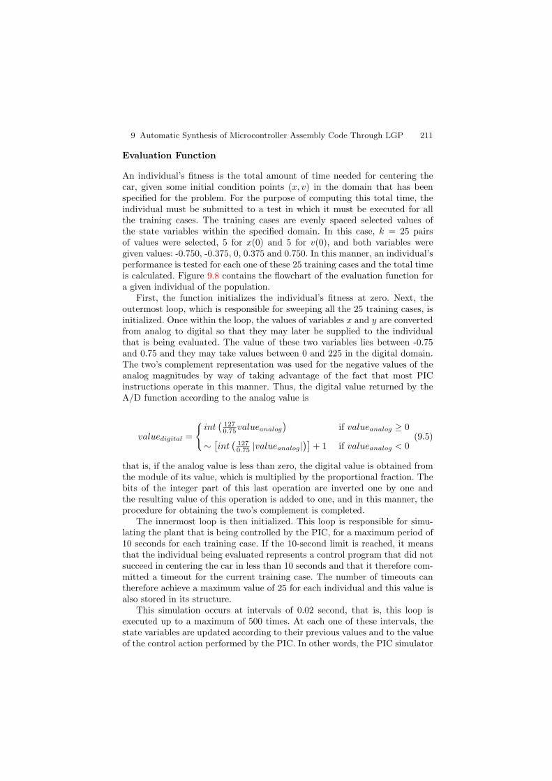
9 Automatic Synthesis of Microcontroller Assembly Code Through LGP 211
Evaluation Function
An individual’s fitness is the total amount of time needed for centering thecar, given some initial condition points (x, v) in the domain that has beenspecified for the problem. For the purpose of computing this total time, theindividual must be submitted to a test in which it must be executed for allthe training cases. The training cases are evenly spaced selected values ofthe state variables within the specified domain. In this case, k = 25 pairsof values were selected, 5 for x(0) and 5 for v(0), and both variables weregiven values: -0.750, -0.375, 0, 0.375 and 0.750. In this manner, an individual’sperformance is tested for each one of these 25 training cases and the total timeis calculated. Figure 9.8 contains the flowchart of the evaluation function fora given individual of the population.
First, the function initializes the individual’s fitness at zero. Next, theoutermost loop, which is responsible for sweeping all the 25 training cases, isinitialized. Once within the loop, the values of variables x and y are convertedfrom analog to digital so that they may later be supplied to the individualthat is being evaluated. The value of these two variables lies between -0.75and 0.75 and they may take values between 0 and 225 in the digital domain.The two’s complement representation was used for the negative values of theanalog magnitudes by way of taking advantage of the fact that most PICinstructions operate in this manner. Thus, the digital value returned by theA/D function according to the analog value is
valuedigital =
int
(1270.75valueanalog
)if valueanalog ≥ 0
∼ [int
(1270.75 |valueanalog|
)]+ 1 if valueanalog < 0
(9.5)
that is, if the analog value is less than zero, the digital value is obtained fromthe module of its value, which is multiplied by the proportional fraction. Thebits of the integer part of this last operation are inverted one by one andthe resulting value of this operation is added to one, and in this manner, theprocedure for obtaining the two’s complement is completed.
The innermost loop is then initialized. This loop is responsible for simu-lating the plant that is being controlled by the PIC, for a maximum period of10 seconds for each training case. If the 10-second limit is reached, it meansthat the individual being evaluated represents a control program that did notsucceed in centering the car in less than 10 seconds and that it therefore com-mitted a timeout for the current training case. The number of timeouts cantherefore achieve a maximum value of 25 for each individual and this value isalso stored in its structure.
This simulation occurs at intervals of 0.02 second, that is, this loop isexecuted up to a maximum of 500 times. At each one of these intervals, thestate variables are updated according to their previous values and to the valueof the control action performed by the PIC. In other words, the PIC simulator

212 Douglas M. Dias et al.
fitness := 0k := 1
k = 25Completion of evaluation
of individual fitness
Initialize state of plant to initial condition for case k
t:=0
t = 10 s
Individual execution by MC simulator:ud(k,t) := Execute(xd(k,t), vd(k,t))
Plant simulation:(x(k,t+1), v(k,t+1)) := Simulate(x(k,t), v(k,t), u(k,t))
fitness := fitness + 0,02
(x(k,t)2+v(k,t)2)1/2
<0,025
t:=t+0,02
k:=k+1
Evaluate fitnessparcel associated
with case k
S
N
S
N
N S
touts:=
touts+1
Fig. 9.8. Flowchart of the evaluation function for the cart-centering problem
takes the digital values xd(k, t) and vd(k, t) of the state variables as its inputsand returns the value of the control variable ud(k, t) as its output. The valueof the control action u(k, t) that will be supplied to the plant simulator isobtained in the following manner: if the value of ud(k, t) is 1, then the valueof u(k, t) will also be 1 because the force to be applied is 1 Newton in thepositive direction; if the value of ud(k, t) is 0, then the value of u(k, t) will be-1 because the force of 1 Newton will be applied in the negative direction. Theplant simulator, in turn, takes the state variables x(k, t) and v(k, t) and thecontrol variable u(k, t), returning the updated values x(k, t+1) and v(k, t+1)of the state variables, which are obtained through equations 9.1, 9.2 and 9.3.

9 Automatic Synthesis of Microcontroller Assembly Code Through LGP 213
Upon completion of one more time interval, the value of 0.02 second is addedto the fitness, which will have a maximum final value of 10 seconds.
As a last processing procedure for this innermost loop, a test is performedfor the purpose of checking if the control action has placed the plant in thefinal state of equilibrium desired, which occurs when the square root of thesum of the squares of position and velocity is lower than 0.025. Otherwise,the simulation continues to be executed for the given training case k until thesystem is put in the state of equilibrium or until the maximum time limit of10 seconds has been reached. At the end of this loop, the fitness parcel relativeto the current case k is obtained. This simulation loop is executed for all thetraining cases and once all theses cases have been completed, the individual’sfitness is finally obtained as being the sum of all theses parcels.
Experiment
Table 9.3 summarizes this experiment and describes its main features andparameters.
Table 9.3. Summary of the evolutionary experiment with the cart-centering prob-lem
Objective: To synthesize an assembly language program that enables aPIC18F452 MC to control a car on a frictionless track so asto center it in a final central position.
Terminal set: X (position), V (velocity) and U (control); A1 and A2 (auxil-iary); PRODH and PRODL (multiplier hardware registers);STATUS (flag register).
Function set: The 22 PIC instructions described in Table 9.2.
Training cases: 25 initial condition points (x,v), selected and evenly spaced,between -0.75 and 0.75. 5 values for x and 5 values for v(-0.750, -0.375; 0; 0.375, 0.750).
Hits: Number of training cases that did not cause a timeout.
Fitness: Sum of the time, over the 25 training cases, taken to centerthe car. When a training case causes a timeout, the contri-bution is of 10 seconds.
Evaluation: The least number of timeouts. As a first tie-breaking crite-rion, the lowest fitness. As a second tie-breaking criterion,the shortest length of the individual.
Main parameters: M = 500. Steady state. Number of individuals processed:400,000, which is equivalent to G = 800. pc = 0.8, pm = 0.4.

214 Douglas M. Dias et al.
In [14], the evaluation of the individual is based solely on its fitness. Thisapproach was also adopted in this paper at first, but upon completion of thefirst experiments, a disadvantage was noticed. When evolution begins, eventhe best individuals are not capable of centering the car for the 25 trainingcases, that is to say, the initial number of timeouts they present is higherthan 20. In this approach, the authors start from the assumption that asfitness diminishes during evolution, the number of timeouts also tends todiminish. This was in fact verified in the first experiments that were carriedout, but only as a tendency, not as a rule. In other words, despite the factthat in some parts of the evolution the number of timeouts diminished asthe fitness also diminished, it was observed that many times the reductionof fitness led to increased timeouts. This revealed that the GP was evolvingindividuals that were less fit, even if this represented individuals with a highernumber of timeouts, which indicates that an individual is less qualified todeal with the training cases. Therefore, an approach was adopted in whichthe individuals are evaluated with regard to the number of timeouts, wherethe tie-breaking criterion is fitness itself. This approach significantly improvedthe GP’s evolutionary performance without affecting the experiment’s initialobjective, which is to promote the evolution of time-optimal control programs.
In this paper, a heuristic on evaluation was developed for the purpose of en-couraging the evolution of individuals with optimized code sizes. This heuris-tic capitalizes on the tournament selection approach that has been adopted,which always compares the individuals’ fitness in pairs. When it is observedthat the individuals have the same fitness value, their lengths are comparedand the one that has the lower value wins the tournament. In this manner,the individual that presents the same performance upon solving the problem,but that does so with a smaller code, is rewarded in detriment of the other.
The experiments revealed that a smaller population causes faster conver-gence, but with a higher final fitness value, while a large population convergesmore slowly, but reaches a lower final fitness value. This fact was also veri-fied in [18]. In this manner, it was decided that M = 500 would be the valuefor population size in this experiment. It was determined, also by experimen-tation, that the crossover and mutation rate values that provided the bestevolutionary performance were, respectively: pc = 0.8 and pm = 0.4.
During the analysis of the evolutionary curve of some of the executions ofthis experiment, it was noticed that convergence occurs before cycle number100,000, which is equivalent to the evaluation of 400,000 individuals since 4individuals are evaluated in each cycle.
Figure 9.9 shows a graph of a preliminary experiment in which the lengthof the individuals was not used as a tie-breaking criterion. Figure 9.10, inturn, shows the graph of the experiment that used the heuristic on the lengthof the individuals. Both graphs represent the average of the results of 10 exe-cutions. It may be noticed that in the first experiment (figure 9.9), the codesize went on growing until it finally reached a near-90 value. This is a famil-iar phenomenon in GP called ”bloat” [5], and it is also one of problems that

9 Automatic Synthesis of Microcontroller Assembly Code Through LGP 215
the literature in this area discusses the most. What happens is that the av-erage size of the individuals tends to increase rapidly during the evolutionaryprocess, as, for example, in [14]. Upon observation of the evolutionary graph ofthe second experiment (figure 9.10), it may be noticed that the bloat problemwas satisfactorily controlled with the use of this heuristic without hamperingthe system’s evolutionary performance.
0
50
100
150
200
250
300
0 10000 20000 30000 40000 50000 60000 70000 80000 90000 100000
Cicles
Fitness
Length
Time outs
Fig. 9.9. Evolution of the cart-centering problem, without control over the lengthof the individuals
The best individual that was evolved in all the executions presented afitness of about 65 seconds for the 25 training cases. In order to find outwhether this individual represented the optimal solution to the problem, anelectronic spreadsheet was used for the purpose of comparing the values thatthe program assigned to the control variable u(t) with the values that it shouldassign according to equation 9.4, which describes time-optimal control. Thiscomparison was carried out for all the 256 points that variables x and vwould be able to assume in the digital domain, which would be equivalentto the -0.75 and 0.75 variation in the analog domain. Actually, the valuesof u(t) obtained by the evolved program, for all these 65,536 points (256 x256), coincided exactly with the values obtained directly from the equation fortime-optimal control. This proves that the evolved program really implementsthe time-optimal control strategy for the problem.
The total evolution (100,000 cycles) time was approximately 3 hours.Around cycle number 7,000, which occurred within about 12 minutes, thefirst individuals that were able to center the car for all the training cases, thatis, the individuals whose number of timeouts equaled zero, began to appear.From this point on, it was noticed that the evolution continues to reduce the
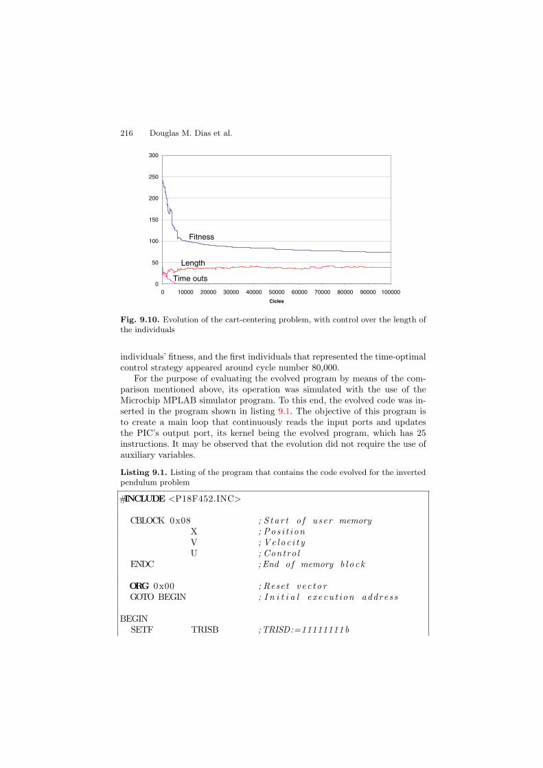
216 Douglas M. Dias et al.
0
50
100
150
200
250
300
0 10000 20000 30000 40000 50000 60000 70000 80000 90000 100000
Cicles
Fitness
Length
Time outs
Fig. 9.10. Evolution of the cart-centering problem, with control over the length ofthe individuals
individuals’ fitness, and the first individuals that represented the time-optimalcontrol strategy appeared around cycle number 80,000.
For the purpose of evaluating the evolved program by means of the com-parison mentioned above, its operation was simulated with the use of theMicrochip MPLAB simulator program. To this end, the evolved code was in-serted in the program shown in listing 9.1. The objective of this program isto create a main loop that continuously reads the input ports and updatesthe PIC’s output port, its kernel being the evolved program, which has 25instructions. It may be observed that the evolution did not require the use ofauxiliary variables.
Listing 9.1. Listing of the program that contains the code evolved for the invertedpendulum problem
#INCLUDE <P18F452.INC>
CBLOCK 0x08 ; S t a r t o f user memoryX ; Pos i t i onV ; Ve l o c i t yU ; Contro l
ENDC ; End o f memory b l o c k
ORG 0x00 ; Reset v e c t o rGOTO BEGIN ; I n i t i a l e xecu t ion address
BEGINSETF TRISB ;TRISD:=11111111 b

9 Automatic Synthesis of Microcontroller Assembly Code Through LGP 217
; Def ine a l l por t B pins; as inpu t s
SETF TRISC ;TRISC:=11111111 b; Define a l l por t C pins; as inpu t s
CLRF TRISD ;TRISB:=00000000 b; Define a l l por t D pins; as ou tpu t s
LOOPCLRF W ;W:=0
; I n i t i a l i z e W r e g i s t e rCLRF PRODH ;PRODH:=0
; I n i t i a l i z e PRODH r e g i s t e rCLRF PRODL ;PRODL:=0
; I n i t i a l i z e PRODL r e g i s t e rMOVFF PORTB, X ;X:=PORTD
; Read por t D ( po s i t i o n )MOVFF PORTC, V ;V:=PORTC
; Read por t C ( v e l o c i t y )
BTFSC X,7 ; S t a r t o f e vo l v ed codeSUBWF V,WBTFSC V,7SUBWF V,FMULWF XINCF V,WADDWF X,FADDWF X,FMULWF PRODH,WSUBWF PRODH,WMULWF XADDWF X,FADDWF X,FSUBWF PRODH,WBTFSC V,7ADDWF X,FBTFSC X,7SETF UMULWF PRODHSUBWF PRODH,WADDWF X,FMULWF XMULWF PRODHBTFSC PRODH,7

218 Douglas M. Dias et al.
SETF U ; End o f e vo l v ed code
MOVFF U, PORTD ;PORTD:=U; Write to por t D ( con t r o l )
GOTO LOOP ; Return to beg inn ing o f loopEND
9.7.2 Inverted Pendulum
The problem of balancing an inverted pendulum in a minimum amount oftime by applying a bang-bang force in one or in another direction is quitea familiar time-optimal control problem and involves an inherently unstablemechanical system. The dynamics of this problem is nonlinear and the prob-lem of balancing the pendulum has been approached in several ways. Someof the approaches involve linear controllers and were not very successful [17].Recently, nonlinear controllers for this problem were studied by researchersin artificial intelligence, evolutionary computing [2][8][11][14] and neural net-works [1]. These nonlinear controllers offer better possibilities for obtaining anoptimal performance in terms of the time required for achieving the objectivestate and the amount of effort that is expended.
The inverted pendulum problem bears a certain similarity to the cart-centering problem in the sense that it involves a car with mass mc movingalong a one-dimensional frictionless track. Additionally, there is an invertedpendulum with mass mp whose axis is on top of the car. The pendulum hasan angle θ and an angular velocity ω. The distance from the mass center ofthe pendulum to its axis is λ.
There is a control variable for this system: a force F of fixed magnitude(bang-bang force) that can be applied to the mass center of the car at eachtime interval so as to accelerate it in the positive or negative directions alongthe track.
This system is shown in figure 9.11 and has four state variables: the car’sposition x along the axis, the car’s velocity v, the angle θ of the pendulum(measured vertically) and the angular velocity ω of the pendulum. In the samemanner as [14] and [8], this case study considers a particular version of thisproblem in which only three of the state variables are controlled and variablex relative to position is not included.
In this hypothetical experiment, the PIC takes the car’s velocity, the pen-dulum’s angle and angular velocity as its inputs and returns the control actionaccording to the values of these inputs. For obtaining the value relative to thecar’s velocity v(t), the signal originating from a potentiometer, which is at-tached to one of the wheels, passes through a differentiator that has beencalibrated to provide a value between -0.2 and 0.2 volts to represent the valueof v(t) between -0.2 and 0.2 meters per second. This analog signal is then con-verted to digital and supplied to the PIC through port D. The value relative

9 Automatic Synthesis of Microcontroller Assembly Code Through LGP 219
AmpAmp
A/DA/D
PotMotor
uv
dx/dtdx/dt A/DA/D
V
F
Porta B
Porta D
Porta C
Porta E
Porta B
Porta D
Porta C
Porta E
dx/dtdx/dt A/DA/D
8
8
8
ω
θ
Pot
θ
ω
x(t)
Fig. 9.11. The inverted pendulum problem controlled by a PIC
to the angle θ(t) is obtained by means of a potentiometer (attached to thependulum’s axis) that is fed and calibrated so as to provide a value between-0.2 and 0.2 volts to represent the value of θ(t) between -0.2 and 0.2 radians.This analog voltage value is then converted to digital and is supplied to thePIC through port B. For obtaining the value relative to the pendulum’s angu-lar velocity ω(t), the signal originating from the potentiometer passes througha differentiator that has been calibrated to provide a value between -0.2 and0.2 volts to represent the value of ω(t) between -0.2 and 0.2 radians per sec-ond. This analog signal is then converted to digital and is supplied to the PICthrough port C. The PIC performs the control u(t) of the car through thepin relative to the least significant bit of port E. Its value is supplied to thecurrent amplifier which, upon receiving the low logical value (0V), activatesthe motor so as to impart to the car a force in the negative direction, andupon receiving the high logical level (5V), activates it imparting a force in thepositive direction to the car.
At each time interval, the selection of the control variable u(t), whichindicates in which direction the force F will be applied, at instant t, brings

220 Douglas M. Dias et al.
about a change in the system’s state variables at instant t + 1. This system’sstate transitions are expressed by nonlinear differential equations. At eachdiscrete time interval t, the current state of the system and the force that isbeing applied at that interval determine the system’s state at the followinginstant.
The pendulum’s angular acceleration Φ(t) at instant t is given by [1] as
Φ(t) =g sin θ + cos θ
−F−mpλωθ2 sin θmc+mp
λ( 43 − mp cos2 θ
mc+mp)
(9.6)
The constants are: the car mass (mc = 0.9 kilogram), the pendulum mass(mp = 0.1 kilogram), the gravity (g = 1.0 meter/sec2), the time interval (t= 0.02 second) and the length of the pendulum (λ = 0.8106 meter). Thependulum’s angular velocity w(t + 1) at instant t + 1 is therefore
ω(t + 1) = ω(t) + τΦ(t) (9.7)
Thus, as a result of the angular acceleration F (t), the angle θ(t + 1) atinstant t + 1 is, with the use of Euler’s integration approximation,
θ(t + 1) = θ(t) + τω(t) (9.8)
The acceleration a(t) of the car on the track is given by
a(t) =F + mpλ(θ2 sin θ − ω cos θ)
mc + mp(9.9)
The velocity v(t + 1) of the car on the track at instant t + 1 is therefore
v(t + 1) = v(t) + τa(t) (9.10)
Evaluation Function
The evaluation function of this case study is similar to the one in the previousstudy. The fitness of an individual is the total amount of time needed forbalancing the pendulum, given some initial condition points (v, θ, ω) in thedomain that has been specified for the problem. For the purpose of computingthis total time, the individual must be submitted to a test in which it mustbe executed for all the training cases. The training cases are evenly spacedselected values of the state variables within the specified domain. In this case,k = 27 values were selected, 3 for v(0), 3 for θ(0) and 3 for ω(0), and thesethree variables took values: -0.2, 0 and 0.2. In this manner, an individual’sperformance is tested for each one of these 27 training cases and the totalamount of time is calculated.
The plant’s simulation time is 6 seconds and if this period is exceeded, atimeout is caused. This simulation occurs at intervals of 0.02 second, that is,

9 Automatic Synthesis of Microcontroller Assembly Code Through LGP 221
this loop is executed up to a maximum of 300 times. It is considered that theplant has reached its state of equilibrium when the square root of the sum ofthe squares of the car’s velocity, of the angle and of the angular velocity ofthe pendulum is lower than 0.07.
Experiment
Table 9.4 summarizes this experiment and describes its main features andparameters.
Table 9.4. Summary of the evolutionary experiment with the inverted pendulumproblem
Objective: To synthesize an assembly language program that enables aPIC18F452 MC to control a car on a track so as to lead aninverted pendulum to a state of equilibrium.
Terminal set: V (car’s velocity), O (angle), w (angular velocity) and U(control); A1 and A2 (auxiliary); PRODH and PRODL (mul-tiplier hardware registers); STATUS (flag register).
Function set: The 22 PIC instructions described in Table 9.2.
Training cases: 27 initial condition points (v, θ, ω), selected and evenlyspaced, between -0.2 and 0.2. There are 3 values for eachvariable: -0.2; 0 and 0.2.
Hits: Number of training cases that did not cause a timeout.
Fitness: Sum of the time, over the 27 training cases, taken to equi-librate the car. When a training case causes a timeout, thecontribution is of 6 seconds.
Evaluation: The least number of timeouts. As a first tie-breaking crite-rion, the lowest fitness. As a second tie-breaking criterion,the shortest length of the individual.
Main parameters: M = 1000. Steady state. Number of processed individuals:400,000, which is equivalent to G = 400. pc = 0.8, pm = 0.4.
The process adopted for evaluating each individual in this case study wasthe same as the one in the previous study. In other words, a significant im-provement was observed in evolutionary performance when the individualswere evaluated with respect to the number of timeouts first, and in case therewas a tie, with regard to the fitness itself. The heuristic on control over thelength of the individuals was also used here since the experiments that werecarried out in the previous case studies had demonstrated that it was satis-factory.

222 Douglas M. Dias et al.
This problem represented increased complexity for the GP, since the sys-tem has three state variables to be controlled and is inherently unstable. As aresult, it became necessary to increase the size of the population to M = 1,000individuals. Each evolution was carried out up to cycle 100,000, hence, 400,000individuals were evaluated. If the GP were generation-based, this would beequivalent to G = 400 generations of 1,000 individuals.
Figure 9.12 shows an evolutionary graph that represents the result of theaverage of 10 executions of the GP.
0
20
40
60
80
100
120
140
160
0 10000 20000 30000 40000 50000 60000 70000 80000 90000 1000
Cicles
Fitness
Length
Time outs
Fig. 9.12. Evolution of the inverted pendulum problem, with control over the lengthof the individuals.
There is no known solution to this problem, neither is there any specific testthat might be applied with a view to establishing that an apparent solutionthat has been obtained is optimal. A pseudo-optimal strategy developed in [15]served as an approximate reference for determining the possible attainment ofa suboptimal value for time. This pseudo-optimal strategy is an approximatedsolution to a linear simplification of the problem. When the initial conditionsconsist of the eight vertices of cube v−θ−ω, it takes this strategy an averageof 2.96 seconds to balance the system. The evolved program, when submittedto the same points, balances the system in 2.84 seconds on the average. Thisshows that the GP was able to synthesize a solution that was better than thebest solution obtained mathematically.
The best individual that was evolved in all the executions presented afitness of approximately 67 seconds for the 27 training cases. The total evolu-tion (100,000 cycles) time was approximately 5 hours. Around cycle number66,000, which occurred within about 3 hours and 20 minutes, the first in-

9 Automatic Synthesis of Microcontroller Assembly Code Through LGP 223
dividuals that were able to balance the system for all the training cases, inother words, the individuals whose number of timeouts equaled 0, began toappear. From this point on, it was noticed that the evolution continues toreduce the individuals’ fitness, and the first individuals that represented theevolved individual’s control strategy appeared around cycle number 78,000.
For the purpose of validating the evolved program, its operation was sim-ulated with the use of the Microchip MPLAB simulator program. To this end,the evolved code was inserted in the program shown in listing 9.2. The ob-jective of this program is to create a main loop that continuously reads theinput ports and updates the PIC’s output port, its kernel being the evolvedprogram, which has 25 instructions. It may be observed that the evolutiondid not require the use of auxiliary variables.
Listing 9.2. Listing of the program that contains the code evolved for the invertedpendulum problem
#INCLUDE <P18F452.INC>
CBLOCK 0x08 ; S t a r t o f user memoryO ; Anglew ; Angular v e l o c i t yV ; Car v e l o c i t yU ; Contro l
ENDC ; End o f memory b l o c k
ORG 0x00 ; Reset v e c t o rGOTO BEGIN ; I n i t i a l e xecu t ion address
BEGINSETF TRISB ;TRISB:=11111111 b
; Define a l l por t B pins; as inpu t s
SETF TRISC ;TRISC:=11111111 b; Define a l l por t C pins; as inpu t s
SETF TRISD ;TRISD:=11111111 b; Define a l l por t D pins; as inpu t s
CLRF TRISE ;TRISB:=00000000 b; Define a l l por t E pins; as ou tpu t s
LOOPCLRF W ;W:=0
; I n i t i a l i z e W r e g i s t e rCLRF PRODH ;PRODH:=0

224 Douglas M. Dias et al.
; I n i t i a l i z e PRODH r e g i s t e rCLRF PRODL ;PRODL:=0
; I n i t i a l i z e PRODL r e g i s t e rMOVFF PORTB, O ;O:=PORTB
; Read por t B ( ang le )MOVFF PORTC, w ;w:=PORTC
; Read por t C ( angu lar v e l o c i t y )MOVFF PORTD, V ;V:=PORTD
; Read por t D ( car v e l o c i t y )
ADDWFC PRODH, F ; S t a r t o f e vo l v ed codeBTFSC STATUS, 0RLCF PRODL, FRLCF w, FRLCF O, WADDWF w, FADDWFC PRODH, FADDWF w, WADDWFC V, WSUBWF PRODL, FMOVFF w, WRLCF U, FSUBWF PRODH, FRLCF PRODL, FADDWF V, WADDWFC V, WRLCF O, WADDWFC PRODL, FCPFSGT VADDWFC PRODL, FCPFSEQ PRODLCPFSGT VSUBWF PRODH, WBTFSS U, 7RLCF U, F ; End o f e vo l v ed code
MOVFF U, PORTE ;PORTE:=U; Write to por t E ( con t r o l )
GOTO LOOP ; Return to beg inn ing o f loopEND

9 Automatic Synthesis of Microcontroller Assembly Code Through LGP 225
9.8 Summary
Systems based on genetic programming make it possible to automaticallysynthesize programs that implement optimal-time control strategies for mi-crocontrollers directly in assembly language. Within this application class, thebest model is the one used in linear genetic programming, in which each chro-mosome is represented by an instruction list. This model makes it possible toevolve programs in assembly language, which is an imperative language. Thiswould not be possible with the use of a tree-based representation because suchrepresentations evolve programs in functional languages only.
The evolution of programs directly in assembly language has proved to beindispensable for two main reasons:
1. Because it represents a device’s lowest possible programming level, it en-abled evolution to find solutions with optimized codes since the evaluationfunctions excelled in programs with smaller amounts of instructions;
2. In terms of evolution time, it made the practical application of the systema viable alternative, since evolution in a higher-level language, such as C,for example, would require the compilation stage, which is executed ateach evaluation, and this would represent a significant increase in thetotal evolution time and make it impossible to use the system in practice.
The case studies discussed here represented the problems one typicallyencounters when dealing with the control of physical systems, such as the factthat the models are nonlinear and the problem of controlling several statevariables through actions performed on one control variable.
As for the final results, the experiments with the case studies demonstratedthat the automatic synthesis system yields a good performance since it wasable to automatically synthesize a control program whose performance wasat least as good as the one found in the literature as a performance qualitybenchmark. The most important aspect of this approach is that the solutionsfound for the control problems were obtained already in the system’s finalimplementation format, that is to say, a program for a microcontroller. Thisresult was obtained directly from the mathematical models of the systemsthat were to be controlled, and other possible intermediate stages between themodeling and implementation stages became unnecessary. In other words, thismethodology eliminates the need for the systems designer to find an optimalor suboptimal solution for the system mathematically and also eliminates themanual task of creating a program that implements this solution.
With regard to synthesis time, this methodology also proves that it cancompete with a human designer because it is able to provide a solution in a fewhours. It is important to point out that the development of control programsinvolving such complex systems as the ones in the case studies presented heremay require a few days to be completed.
The total time spent in synthesis is still considered relatively long. Thereare several alternatives for reducing it.
226 Douglas M. Dias et al.
First, develop an algorithm that identifies the parts of the program thatdo not present any influence on the calculation of the output(s), for all thepossible inputs (introns). This algorithm would be based on the study byBrameier & Banzhaf [6], where the complexity level of the algorithm developedis, in the worst case, O(n), n being the length of the individual. On the onehand, this approach would reduce the total evolutionary time because theintrons would no longer be interpreted by the MC simulator. On the other,it would improve the throughput of the mutation operator, which would onlybe applied in the effective code sections and thus increase the velocity of theevolution.
Another possibility is to investigate the use of several demes [20] so as todelay the convergence of the GP as much as possible, since a conversion ata later time may represent the synthesis of programs with more optimizedcontrol performances. An additional alternative that may be considered isthe use of MC instructions that make it possible to create execution loopsthat might contribute in some additional way to the quality of the evolvedprograms. This would also involve studying a manner by which to deal withundesirable infinite loops that might occur.
An additional alternative that may be considered is the use of MC instruc-tions that make it possible to create execution loops that might contribute insome additional way to the quality of the evolved programs. This would alsoinvolve studying a manner by which to deal with undesirable infinite loopsthat might occur.
References
1. C. W. Anderson. Learning to control an inverted pendulum using neural net-works. IEEE Control Systems Magazine, pages 31–37, 1989. 218, 220
2. Peter J. Angeline. An alternative to indexed memory for evolving programswith explicit state representations. In John R. Koza, Kalyanmoy Deb, MarcoDorigo, David B. Fogel, Max Garzon, Hitoshi Iba, and Rick L. Riolo, editors,Genetic Programming 1997: Proceedings of the Second Annual Conference, pages423–430, Stanford University, CA, USA, 1997. Morgan Kaufmann. 218
3. K. J. Astrm and B. Wittenmark. Computer-Controlled systems: theory anddesign. Prentice-Hall, New Jersey, 1997. 199
4. M. Athans and P. L. Falb. Optimal Control: An Introduction to the Theory andIts Applications. McGraw-Hill Book Company, New York, 1966. 199, 208, 210
5. Wolfgang Banzhaf, Peter Nordin, Robert E. Keller, and Frank D. Francone. Ge-netic Programming – An Introduction; On the Automatic Evolution of ComputerPrograms and its Applications. Morgan Kaufmann, dpunkt.verlag, 1998. 196, 197, 204, 205, 214
6. Markus Brameier and Wolfgang Banzhaf. Effective linear genetic programming.Technical report, Department of Computer Science, University of Dortmund,44221 Dortmund, Germany, 2001. 203, 204, 226
7. Markus Brameier, Wolfgang Kantschik, Peter Dittrich, and Wolfgang Banzhaf.SYSGP – A C++ library of different GP variants. Technical Report CI-98/48,Collaborative Research Center 531, University of Dortmund, Germany, 1998. 201

9 Automatic Synthesis of Microcontroller Assembly Code Through LGP 227
8. Kumar Chellapilla. Automatic generation of nonlinear optimal control laws forbroom balancing using evolutionary programming. In Proceedings of the 1998IEEE World Congress on Computational Intelligence, pages 195–200, Anchor-age, Alaska, USA, 1998. IEEE Press. 218
9. Nichael Lynn Cramer. A representation for the adaptive generation of simplesequential programs. In John J. Grefenstette, editor, Proceedings of an Interna-tional Conference on Genetic Algorithms and the Applications, pages 183–187,Carnegie-Mellon University, Pittsburgh, PA, USA, 24-26 July 1985. 195, 196
10. Ronald L. Crepeau. Genetic evolution of machine language software. In Jus-tinian P. Rosca, editor, Proceedings of the Workshop on Genetic Programming:From Theory to Real-World Applications, pages 121–134, Tahoe City, California,USA, 1995. 196, 197
11. D. B. Fogel. A ’correction’ to some cart-pole experiments. In T. Baeck L. J. Fo-gel, P. J. Fogel, editor, Evolutionary Programming V: Proceedings of the FifthAnnual Conference on Evolutionary Programming, pages 67–71, Cambridge,MA, 1996. MIT Press. 218
12. Lorenz Huelsbergen. Toward simulated evolution of machine language iteration.In John R. Koza, David E. Goldberg, David B. Fogel, and Rick L. Riolo, editors,Genetic Programming 1996: Proceedings of the First Annual Conference, pages315–320, Stanford University, CA, USA, 28–31 July 1996. MIT Press. 196
13. Kenneth E. Kinnear, Jr. Evolving a sort: Lessons in genetic programming. InProceedings of the 1993 International Conference on Neural Networks, volume 2,pages 881–888, San Francisco, USA, 1993. IEEE Press. 206
14. John R. Koza. Genetic Programming: On the Programming of Computers byMeans of Natural Selection. MIT Press, Cambridge, MA, USA, 1992. 201, 208, 210, 214, 215, 218
15. John R. Koza and Martin A. Keane. Cart centering and broom balancing bygenetically breeding populations of control strategy programs. In Proceedings ofInternational Joint Conference on Neural Networks, volume I, pages 198–201,Washington, 1990. Lawrence Erlbaum. 222
16. Microchip. PIC18FXX Data Sheet, 2002. http://www.microchip.com. 20017. S. Mori, H. Nishihara, and K. Furuta. Control of unstable mechanical system-
control of pendulum. Int. J. Control, pages 673–692, 1976. 21818. Peter Nordin. A compiling genetic programming system that directly manipu-
lates the machine code. In Kenneth E. Kinnear, Jr., editor, Advances in GeneticProgramming, chapter 14, pages 311–331. MIT Press, 1994. 196, 201, 214
19. Peter Nordin. Evolutionary Program Induction of Binary Machine Code and itsApplication. Krehl-Verlag, Mnster, Germany, 1997. 196, 202, 203, 205
20. Peter Nordin, Frank Hoffmann, Frank D. Francone, Markus Brameier, andWolfgang Banzhaf. AIM-GP and parallelism. In Peter J. Angeline, ZbyszekMichalewicz, Marc Schoenauer, Xin Yao, and Ali Zalzala, editors, Proceed-ings of the Congress on Evolutionary Computation, volume 2, pages 1059–1066,Mayflower Hotel, Washington D.C., USA, 1999. IEEE Press. 226
21. Katsuhiko Ogata. Modern Control Engineering. Prentice-Hall, 1997. 194, 195, 199

Index
ambiguous, 81, 83, 102assembly, 195, 197, 202automata, 82, 90, 92, 93, 101, 102automatic programming, 40Automatically Defined Functions, 21,
22, 26, 36, 37, 39, 40, 42, 46, 47,51, 52, 54
automatically defined functions, 178
building blocks, 23, 25, 49
cells, 36, 38, 51, 55cellular system, 26, 37, 54, 55CGP, 1, 18chromosomes, 21, 27circuit encoding, 149classification, 33, 114closure property, 108code reuse, 26, 36, 47, 49controller
action selection, 187, 190hierarchial controller, 186subsumption controller, 186, 188
crossover, 22, 23, 25, 34, 109
data modelling, 129decision trees, 36development, 26, 36
evolution, 21–23, 25, 26, 29, 34, 36, 37,40–42, 44, 46–48, 55
Evolutionary Computation, 105evolutionary hardware, 149–151evolvability, 29
expression tree, 107expression trees, 21, 25, 27
fitness, 26fitness cases, 26, 40, 42fitness function, 41, 109
GADS, 1, 15, 19GE, 1gene domains, 33gene duplication, 46Gene Expression Algorithm, 42Gene Expression Programming, 21, 22,
25–27, 29, 31, 32, 34, 36, 46, 54,55
gene recombination, 46gene transposition, 46genes, 26, 28, 30genetic algorithm, 183Genetic Algorithms, 21, 22, 25genetic algorithms, 1, 2, 5, 12, 19genetic code, 27genetic operators, 25, 26, 29, 34, 54Genetic Programming, 21, 22, 25, 34,
36, 39, 40, 54, 105genetic programming, 1, 2, 12, 19, 81,
83, 92, 102, 133, 138, 197, 227genic terminals, 37genotype, 22, 25, 28, 29genotype/phenotype systems, 21, 22,
26, 29GEP, 15–17GP, 105–107

230 Index
head domain, 30, 37homeotic genes, 36, 37, 54
intrusion, 57–59, 61, 62inversion, 22, 25, 31, 34
K-expressions, 28, 29, 32Karva language, 26, 28Khepera robot, 175
learning, 181LGP, 57, 63, 64, 141, 143, 145linear genome, 22, 25, 26, 32, 54linking, 32, 33, 40, 42linking functions, 32, 37
mathematical modelling, 106MEP, 63–66, 73, 75, 133, 134, 136, 145microcontroller, 196, 197, 200multicellular systems, 26, 37, 46, 50, 55multigenic chromosomes, 32multigenic systems, 32, 36, 37, 44, 51,
54, 55mutation, 22, 24, 25, 30, 31, 34, 110
neural networks, 36, 181, 183neuron, 181neutral regions, 44, 46, 48noncoding regions, 28, 29, 46nonlinear genome, 22
open reading frames, 28, 30, 32overlapping, 81, 82, 84, 90, 91
parameter optimization, 33, 36parse trees, 22, 24–26, 42, 47, 55pattern matching, 81–83, 101, 102permutation, 24phenotype, 22, 25, 27, 28
phenotype threshold, 26polynomial induction, 36posttranslational interaction, 32prediction, 121
random numerical constants, 34, 39, 52,55
recombination, 31, 34relative error, 41replicators, 22
search operators, 22, 26, 31search space, 21, 25selection environment, 26selection method, 109selection range, 41sensor, 176set of functions, 109set of terminals, 109sextic polynomial problem, 21, 40simulation, 185solution space, 26static linking, 44, 47, 51, 54, 55sub-population, 179symbolic regression, 36, 106syntactic closure, 23, 29synthesis, 227, 228
tail domain, 30, 34, 37TGP, 1, 15, 18translation, 27transposition, 25, 31, 34traversal order, 81–83, 86, 90, 91, 93,
102tuning algorithm, 112
unicellular systems, 46, 47, 55unigenic systems, 32, 42

Index
Ajith Abraham, 57, 132
Candida Ferreira, 21Crina Grosan, 57, 132
Douglas Mota Dias, 194
Ewa Szpunar-Huk, 105
Halina Kwasnicka, 105
Jose F. M. Amaral, 194
Luiza de Macedo Mourelle, 1, 80, 149
Marco Aurelio C. Pacheco, 194
Michael Botros, 174
Nadia Nedjah, 1, 80, 149

Reviewer List
Adriane Serapiao John R. Koza
Ajith Abraham Julian F. Miller
Ali Afzalian Kalyanmoy Deb
Antonio Romeiro Sapienza Luiza M. Mourelle
Carlos A. C. Coello Marco Aurelio C. Pacheco
Claudia Martins Silva Marley M. Vellasco
Dirk Buche Nadia Nedjah
El-Ghazali Talbi Peter Dittrich
Evaristo Chalbaud Biscaia Jr. Phillip A. Laplante
Felipe G. M. Franca Radu-Emil Precup
Gregory Hornby Ricardo S. Zebulum
Hitoshi Iba Ricardo Tansheit
Ismat Beg Saeid Abbasbandy
Janusz Kacprzyk Tapabrata Ray
Joao A. Vasconcelos Tim Hendtlass
Johan Andersson Wolfgang Banzhaf