5/03/2014

1

Non Linear Programming

System Modelling

Anna Maria Sri Asih Department of Mechanical & Industrial Engineering

Gadjah Mada University

Include at least one nonlinear function: objective function, or some or all of the constraints Many systems are inherently nonlinear (i.e. EOQ, price

elasticity, etc.) Solution techniques involve searching a solution surface

for high or low points need advanced maths NLP models are much more difficult to optimize

compared to LP

Non-Linear Programming (NLP)

Hard to distinguish a local optimum from a global optimum

NLP: difficult to optimize?

Local optimum: feasible point with better value than any others in a small neighbourhood around it

Global optimum:

feasible point with the best value of objective function anywhere in the feasible region

Common available information (i) The point x itself

(ii) The value of objective function at x

(iii) The values of the constraint functions at x

(iv) The gradient at x (1st derivative)

(v) The Hessian matrix (2nd derivative)

Enough to recognize:

local maximum or

local minimum

Better local max/min ?

How to get there?

Optima are not restricted to extreme points

NLP: difficult to optimize?

LP: check extreme point / corner point of the feasible region

NLP: an optimum (local or global) COULD BE ANYWHERE: at an extreme point, along an edge of the feasible region, or in the interior of the feasible region

Required: n+1 dimensions to illustrate an n-dimensional function

Contour lines: lines that connect all points that all have the same value of the function

Optimum is in the interior of the feasible region (case: local maximum)

5/03/2014

2

There may be multiple disconnected feasible regions

NLP: difficult to optimize?

If we are able to find an optimum within a particular feasible region

how do we know that there isn’t some other disconnected feasible region that haven’t been found/explored?

Different starting point may lead to different final solutions

NLP: difficult to optimize?

Common algorithm: (i) chooses a direction for search and then (ii) finds the best value of the objective function in that direction, and

then (iii) repeat the process until no improvement in the value of the objective

function Multiple different valleys starting a some other point may return in a different final solution point and objective function value (even worse in discontiguous feasible region) Option: restarts fro many different initial points time consuming

There is no definite determination of the outcome

NLP: difficult to optimize?

Outcome in LP:

(i) The model is feasible and there is a globally optimum solution point

(ii) The model is feasible but unbounded

(iii) The model is infeasible

In NLP, the solver:

• Is not able to say whether the point is a global minimum

• May continue improving the value of the objective function for a long time, but will not be able to say whether the model is unbounded

• Is not able to guarantee that the model is actually infeasible if no feasible solution is found

It uses a complex math theory and numerous solution algorithms

NLP: difficult to optimize?

How do we decide which algorithm to apply, and can we follow the complex steps correctly ?

It is difficult to determine whether the conditions to apply a particular solver are met

many solution algorithms require that the functions in the model have particular characteristic, which could relate to their algebraic structure (e.g. quadratic, polynomial, etc.). Or their shape (e.g. curve up or curve down everywhere)

Difficult to determine whether these conditions are satisfied or not?

Different algorithms and solvers arrive at different solutions for the same formulation

NLP: difficult to optimize?

Each algorithm: different trajectory from initial point to the final point that is the output of the solution.

Different algorithms may terminate at different local optima, and hence will return different solutions, even for the exact same

formulation and initial point

5/03/2014

3

Look for a simpler formulation, i.e. nonlinear function linear function Know the characteristics of your model before choosing a

solution algorithm provide a good starting point (i.e. previous solution, trial

error simple analysis, find methods for selecting starting points) Put reasonable bounds on all variables narrow the search

space for the solver

What can we do?

A function f(x1,x2,…xn) is separable if it can be written as a sum of functions of a single variable:

𝒇(𝒙𝟏, 𝒙𝟐…𝒙𝒏) = 𝒇𝒊(𝒙𝒊)𝒏𝒊=𝟏

Examples:

Separable Programming

Bricker, D.L. University of Iowa

Separable Not separable

𝑥1 + 2ln(𝑥2) x1x2 + x3

x12 + 3x1 + 6x2 – x2

2 5x1/x2 – x1

We can approximate a nonlinear separable function by a piecewise-linear function:

Separable Programming

Bricker, D.L. University of Iowa

Two ways to formulate piecewise-linear programming problem as a Linear-Programming problem: “lambda” () formulation “delta” () formulation

Suppose that f(z) is a convex function.

Let 0, 1,… be specified “grid points”, and 0, 1,… be “weights” where 𝑖 = 1,𝑖 ≥ 0𝑖

Bricker, D.L. University of Iowa

Any value of z in the interval between the left-most and the right-most grid point may be expressed as a “convex combination” of the grid points:

Bricker, D.L. University of Iowa

With the same “weights” used in the convex combination of the grid points (z= 00 + 11 + 22 + 33),

We approximate f(z) as a convex combination of the function values at the grid points

Bricker, D.L. University of Iowa

Example: see the figure Suppose: f(z) is a convex, piecewise linear function. Consider the various convex combinations of grid points yielding z = 1.75

Different convex combinations of the grid points:

Resulting in different approximation of f(z)

5/03/2014

4

Bricker, D.L. University of Iowa

The point 𝑖𝑖,𝑖 𝑖𝑓(𝑖)𝑖 lies on a chord of the graph which is on or above the graph.

So 𝑖𝑓(𝑖)𝑖 is in general an overestimate of f(z).

Bricker, D.L. University of Iowa

Bricker, D.L. University of Iowa Bricker, D.L. University of Iowa

Bricker, D.L. University of Iowa

The best convex combination to approximate f(z) is :

the one which assigns positive weights only to the grid points

immediately to the left and right of z

Bricker, D.L. University of Iowa

The convex combination which yields the LOWEST value for

f(1.75) uses only two ADJACENT grid points !

5/03/2014

5

Bricker, D.L. University of Iowa

When minimizing a convex function f(z) by choosing the weights in the convex combination, then…

…at most TWO i’s will be positive, and these will be weights of adjacent grid points !

What if f(z) is NOT convex ?

Bricker, D.L. University of Iowa

When f(z) is not convex,

the chords do not all lie on or above the graph,

and one may choose convex combinations of grid points

yielding approximations of f(z) which are underestimates of

the function

Bricker, D.L. University of Iowa

For example:

in this figure the lowest (and the worst) estimate of f(3) as a convex combination of 1 and 4 :

3 = 11 + 44

with f(3) is approximated by

1f(1) + 4f(4)

Bricker, D.L. University of Iowa

For non-convex function, or where it is not known whether or not they are convex, linear programming is not sufficient.

Separable programming can be used but no more than a local optimum can be guaranteed.

It s often possible to solve such a model a number of times using different strategies to obtain different local optima.

Most global optimization techniques use local optimization routines in their operation

start by looking at local optimization

Local optimization of NLP

To start:

Simplest possible case: one-dimensional unconstrained function

one NLP objective function

no constraints (“unconstrained”)

one variable

Computer method’s point of view:

It only has individual points and associated objective function values that it calculates

What it sees after the first point it tests looks something like figure above?

Various test points algorithm leads to local optimum

5/03/2014

6

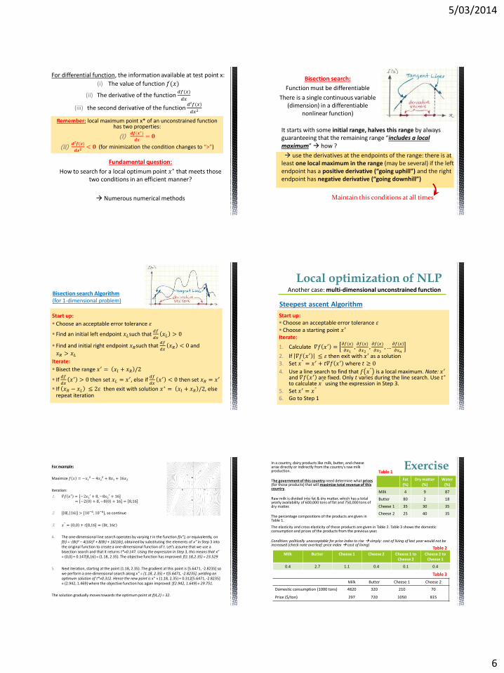
For differential function, the information available at test point x:

(i) The value of function 𝑓(𝑥)

(ii) The derivative of the function 𝑑𝑓(𝑥)

𝑑𝑥

(iii) the second derivative of the function 𝑑2𝑓(𝑥)

𝑑𝑥2

Fundamental question:

How to search for a local optimum point 𝑥∗that meets those two conditions in an efficient manner?

Numerous numerical methods

Remember: local maximum point x* of an unconstrained function has two properties:

(i)𝒅𝒇(𝒙∗)

𝒅𝒙= 𝟎

(ii)𝒅𝟐𝒇(𝒙)

𝒅𝒙𝟐< 𝟎 (for minimization the condition changes to “>”)

Bisection search:

Function must be differentiable

There is a single continuous variable (dimension) in a differentiable

nonlinear function)

Maintain this conditions at all times

It starts with some initial range, halves this range by always guaranteeing that the remaining range “includes a local maximum” how ?

use the derivatives at the endpoints of the range: there is at least one local maximum in the range (may be several) if the left endpoint has a positive derivative (“going uphill”) and the right endpoint has negative derivative (“going downhill”)

Start up:

Choose an acceptable error tolerance 𝜀

Find an initial left endpoint 𝑥𝐿such that 𝑑𝑓

𝑑𝑥𝑥𝐿 > 0

Find and initial right endpoint 𝑥𝑅such that 𝑑𝑓

𝑑𝑥𝑥𝑅 < 0 and

𝑥𝑅 > 𝑥𝐿

Iterate:

Bisect the range 𝑥′ = 𝑥𝑙 + 𝑥𝑅 /2

If 𝑑𝑓

𝑑𝑥𝑥′ > 0 then set 𝑥𝐿 = 𝑥

′, else if 𝑑𝑓

𝑑𝑥𝑥′ < 0 then set 𝑥𝑅 = 𝑥

′

If 𝑥𝑅 − 𝑥𝐿 ≤ 2𝜀 then exit with solution 𝑥∗ = 𝑥𝑙 + 𝑥𝑅 /2, else repeat iteration

Bisection search Algorithm (for 1-dimensional problem)

Another case: multi-dimensional unconstrained function

Local optimization of NLP

Start up: Choose an acceptable error tolerance 𝜀 Choose a starting point 𝑥′ Iterate:

1. Calculate 𝛻𝑓 𝑥′ =𝜕𝑓(𝑥)

𝜕𝑥1,𝜕𝑓(𝑥)

𝜕𝑥2,𝜕𝑓(𝑥)

𝜕𝑥3, …

𝜕𝑓(𝑥)

𝜕𝑥𝑛

2. If 𝛻𝑓 𝑥′ ≤ 𝜀 then exit with 𝑥′ as a solution 3. Set 𝑥" = 𝑥′ + 𝑡𝛻𝑓 𝑥′ where 𝑡 ≥ 0

4. Use a line search to find that 𝑓 𝑥" is a local maximum. Note: 𝑥′ and 𝛻𝑓 𝑥′ are fixed. Only 𝑡 varies during the line search. Use 𝑡∗ to calculate 𝑥" using the expression in Step 3.

5. Set 𝑥′ = 𝑥" 6. Go to Step 1

Steepest ascent Algorithm

For example:

Maximize 𝑓 𝑥 = −𝑥12 − 4𝑥2

2 + 8𝑥1 + 16𝑥2

Iteration:

1. 𝛻𝑓 𝑥′ = −2𝑥1′ + 8,−8𝑥2

′ + 16 = −2 0 + 8, −8 0 + 16 = 8,16

2. 8 , 16 > [10−6 , 10−6], so continue

3. 𝑥" = 0,0 + 𝑡 8,16 = 8𝑡, 16𝑡

4. The one-dimensional line search operates by varying t in the function f(x”), or equivalently, on f(t) = -(8t)2 – 4(16t)2 + 8(8t) + 16(16t), obtained by substituting the elements of x” in Step 3 into the original function to create a one-dimensional function of t. Let’s assume that we use a bisection search and that it returns t*=0.147. Using the expression in Step 3, this means that x” = (0,0) + 0.147[8,16] = (1.18, 2.35). The objective function has improved: f(1.18,2.35) = 23.529

5. Next iteration, starting at the point (1.18, 2.35). The gradient at this point is [5.6471, -2.8235] so we perform a one-dimensional search along x” = (1.18, 2.35) + t[5.6471, -2.8235], yielding an optimum solution of t*=0.312. Hence the new point is x” = (1.18, 2.35) + 0.312[5.6471, -2.8235] = (2.942, 1.469) where the objective function has again improved: f(2.942, 1.649) = 29.751.

The solution gradually moves towards the optimum point at f(4,2) = 32.

In a country, dairy products like milk, butter, and cheese arise directly or indirectly from the country’s raw milk production. The government of this country need determine what prices (for those products) that will maximize total revenue of this country. Raw milk is divided into fat & dry matter, which has a total yearly availability of 600,000 tons of fat and 750,000 tons of dry matter. The percentage compositions of the products are given in Table 1.

Exercise Fat (%)

Dry matter (%)

Water (%)

Milk 4 9 87

Butter 80 2 18

Cheese 1 35 30 35

Cheese 2 25 40 35

Milk Butter Cheese 1 Cheese 2 Cheese 1 to Cheese 2

Cheese 2 to Cheese 1

0.4 2.7 1.1 0.4 0.1 0.4

The elasticity and cross elasticity of those products are given in Table 2. Table 3 shows the domestic consumption and prices of the products from the previous year. Condition: politically unacceptable for price index to rise simply: cost of living of last year would not be increased (check note overleaf: price index cost of living)

Table 1

Table 2

Milk Butter Cheese 1 Cheese 2

Domestic consumption (1000 tons) 4820 320 210 70

Price ($/ton) 297 720 1050 815

Table 3

5/03/2014

7

Exercise Price elasticity of demand:

how much percentage of demand changes in response to 1 percent change in price (note: “-”)

𝐸 = 𝑝𝑒𝑟𝑐𝑒𝑛𝑡𝑎𝑔𝑒𝑑𝑒𝑐𝑟𝑒𝑎𝑠𝑒𝑖𝑛𝑑𝑒𝑚𝑎𝑛𝑑

𝑝𝑒𝑟𝑐𝑒𝑛𝑡𝑎𝑔𝑒𝑖𝑛𝑐𝑟𝑒𝑎𝑠𝑒𝑖𝑛𝑝𝑟𝑖𝑐𝑒

Cross elasticity of demand degree of substitution in consumer demand depending on the relative prices

𝐸𝐴𝐵 =𝑝𝑒𝑟𝑐𝑒𝑛𝑡𝑎𝑔𝑒𝑖𝑛𝑐𝑟𝑒𝑎𝑠𝑒𝑖𝑛𝑑𝑒𝑚𝑎𝑛𝑑𝑓𝑜𝑟𝐴

𝑝𝑒𝑟𝑐𝑒𝑛𝑡𝑎𝑔𝑒𝑖𝑛𝑐𝑟𝑒𝑎𝑠𝑒𝑖𝑛𝑝𝑟𝑖𝑐𝑒𝑓𝑜𝑟𝐵

Price index to measure the economy’s price level or a cost of living ( expensive/cheap country ?)

Exercise Build:

1. Objective function

2. Constraints: a. Limitation on availabilities of fat and dry matter

Steps: 1st : do without elasticity effect

2nd : include elasticity effect

a. Price index limitation

b. Non-negativity