3 Introduction to Linear Programming - OHIO Personal Websites

24

3Introduction to LinearProgramming

The development of linear programming has been ranked among the most important sci-entific advances of the mid-20th century, and we must agree with this assessment. Its im-pact since just 1950 has been extraordinary. Today it is a standard tool that has saved manythousands or millions of dollars for most companies or businesses of even moderate sizein the various industrialized countries of the world; and its use in other sectors of societyhas been spreading rapidly. A major proportion of all scientific computation on comput-ers is devoted to the use of linear programming. Dozens of textbooks have been writtenabout linear programming, and published articles describing important applications nownumber in the hundreds.

What is the nature of this remarkable tool, and what kinds of problems does it ad-dress? You will gain insight into this topic as you work through subsequent examples. How-ever, a verbal summary may help provide perspective. Briefly, the most common type ofapplication involves the general problem of allocating limited resources among competingactivities in a best possible (i.e., optimal) way. More precisely, this problem involves se-lecting the level of certain activities that compete for scarce resources that are necessaryto perform those activities. The choice of activity levels then dictates how much of eachresource will be consumed by each activity. The variety of situations to which this de-scription applies is diverse, indeed, ranging from the allocation of production facilities toproducts to the allocation of national resources to domestic needs, from portfolio selectionto the selection of shipping patterns, from agricultural planning to the design of radiationtherapy, and so on. However, the one common ingredient in each of these situations is thenecessity for allocating resources to activities by choosing the levels of those activities.

Linear programming uses a mathematical model to describe the problem of concern.The adjective linear means that all the mathematical functions in this model are requiredto be linear functions. The word programming does not refer here to computer program-ming; rather, it is essentially a synonym for planning. Thus, linear programming involvesthe planning of activities to obtain an optimal result, i.e., a result that reaches the speci-fied goal best (according to the mathematical model) among all feasible alternatives.

Although allocating resources to activities is the most common type of application,linear programming has numerous other important applications as well. In fact, any prob-lem whose mathematical model fits the very general format for the linear programmingmodel is a linear programming problem. Furthermore, a remarkably efficient solution pro-

cedure, called the simplex method, is available for solving linear programming problemsof even enormous size. These are some of the reasons for the tremendous impact of lin-ear programming in recent decades.

Because of its great importance, we devote this and the next six chapters specificallyto linear programming. After this chapter introduces the general features of linear pro-gramming, Chaps. 4 and 5 focus on the simplex method. Chapter 6 discusses the furtheranalysis of linear programming problems after the simplex method has been initially ap-plied. Chapter 7 presents several widely used extensions of the simplex method and intro-duces an interior-point algorithm that sometimes can be used to solve even larger linear pro-gramming problems than the simplex method can handle. Chapters 8 and 9 consider somespecial types of linear programming problems whose importance warrants individual study.

You also can look forward to seeing applications of linear programming to other ar-eas of operations research (OR) in several later chapters.

We begin this chapter by developing a miniature prototype example of a linear pro-gramming problem. This example is small enough to be solved graphically in a straight-forward way. The following two sections present the general linear programming modeland its basic assumptions. Sections 3.4 and 3.5 give some additional examples of linearprogramming applications, including three case studies. Section 3.6 describes how linearprogramming models of modest size can be conveniently displayed and solved on a spread-sheet. However, some linear programming problems encountered in practice require trulymassive models. Section 3.7 illustrates how a massive model can arise and how it can stillbe formulated successfully with the help of a special modeling language such as MPL(described in this section) or LINGO (described in the appendix to this chapter).

3.1 PROTOTYPE EXAMPLE 25

The WYNDOR GLASS CO. produces high-quality glass products, including windows andglass doors. It has three plants. Aluminum frames and hardware are made in Plant 1, woodframes are made in Plant 2, and Plant 3 produces the glass and assembles the products.

Because of declining earnings, top management has decided to revamp the company’sproduct line. Unprofitable products are being discontinued, releasing production capacityto launch two new products having large sales potential:

Product 1: An 8-foot glass door with aluminum framingProduct 2: A 4 � 6 foot double-hung wood-framed window

Product 1 requires some of the production capacity in Plants 1 and 3, but none in Plant2. Product 2 needs only Plants 2 and 3. The marketing division has concluded that thecompany could sell as much of either product as could be produced by these plants. How-ever, because both products would be competing for the same production capacity in Plant3, it is not clear which mix of the two products would be most profitable. Therefore, anOR team has been formed to study this question.

The OR team began by having discussions with upper management to identify man-agement’s objectives for the study. These discussions led to developing the following def-inition of the problem:

Determine what the production rates should be for the two products in order to maximizetheir total profit, subject to the restrictions imposed by the limited production capacities

3.1 PROTOTYPE EXAMPLE

available in the three plants. (Each product will be produced in batches of 20, so the pro-duction rate is defined as the number of batches produced per week.) Any combinationof production rates that satisfies these restrictions is permitted, including producing noneof one product and as much as possible of the other.

The OR team also identified the data that needed to be gathered:

1. Number of hours of production time available per week in each plant for these newproducts. (Most of the time in these plants already is committed to current products,so the available capacity for the new products is quite limited.)

2. Number of hours of production time used in each plant for each batch produced ofeach new product.

3. Profit per batch produced of each new product. (Profit per batch produced was cho-sen as an appropriate measure after the team concluded that the incremental profit fromeach additional batch produced would be roughly constant regardless of the total num-ber of batches produced. Because no substantial costs will be incurred to initiate theproduction and marketing of these new products, the total profit from each one is ap-proximately this profit per batch produced times the number of batches produced.)

Obtaining reasonable estimates of these quantities required enlisting the help of keypersonnel in various units of the company. Staff in the manufacturing division providedthe data in the first category above. Developing estimates for the second category of datarequired some analysis by the manufacturing engineers involved in designing the pro-duction processes for the new products. By analyzing cost data from these same engineersand the marketing division, along with a pricing decision from the marketing division, theaccounting department developed estimates for the third category.

Table 3.1 summarizes the data gathered.The OR team immediately recognized that this was a linear programming problem

of the classic product mix type, and the team next undertook the formulation of the cor-responding mathematical model.

Formulation as a Linear Programming Problem

To formulate the mathematical (linear programming) model for this problem, let

x1 � number of batches of product 1 produced per week

x2 � number of batches of product 2 produced per week

Z � total profit per week (in thousands of dollars) from producing these two products

Thus, x1 and x2 are the decision variables for the model. Using the bottom row of Table3.1, we obtain

Z � 3x1 � 5x2.

The objective is to choose the values of x1 and x2 so as to maximize Z � 3x1 � 5x2, sub-ject to the restrictions imposed on their values by the limited production capacities avail-able in the three plants. Table 3.1 indicates that each batch of product 1 produced perweek uses 1 hour of production time per week in Plant 1, whereas only 4 hours per weekare available. This restriction is expressed mathematically by the inequality x1 � 4. Simi-larly, Plant 2 imposes the restriction that 2x2 � 12. The number of hours of production

26 3 INTRODUCTION TO LINEAR PROGRAMMING

time used per week in Plant 3 by choosing x1 and x2 as the new products’ production rateswould be 3x1 � 2x2. Therefore, the mathematical statement of the Plant 3 restriction is3x1 � 2x2 � 18. Finally, since production rates cannot be negative, it is necessary to re-strict the decision variables to be nonnegative: x1 � 0 and x2 � 0.

To summarize, in the mathematical language of linear programming, the problem isto choose values of x1 and x2 so as to

Maximize Z � 3x1 � 5x2,

subject to the restrictions

3x1 � 2x2 � 43x1 � 2x2 � 123x1 � 2x2 � 18

and

x1 � 0, x2 � 0.

(Notice how the layout of the coefficients of x1 and x2 in this linear programming modelessentially duplicates the information summarized in Table 3.1.)

Graphical Solution

This very small problem has only two decision variables and therefore only two dimen-sions, so a graphical procedure can be used to solve it. This procedure involves con-structing a two-dimensional graph with x1 and x2 as the axes. The first step is to identifythe values of (x1, x2) that are permitted by the restrictions. This is done by drawing eachline that borders the range of permissible values for one restriction. To begin, note thatthe nonnegativity restrictions x1 � 0 and x2 � 0 require (x1, x2) to lie on the positive sideof the axes (including actually on either axis), i.e., in the first quadrant. Next, observe thatthe restriction x1 � 4 means that (x1, x2) cannot lie to the right of the line x1 � 4. Theseresults are shown in Fig. 3.1, where the shaded area contains the only values of (x1, x2)that are still allowed.

In a similar fashion, the restriction 2x2 � 12 (or, equivalently, x2 � 6) implies thatthe line 2x2 � 12 should be added to the boundary of the permissible region. The finalrestriction, 3x1 � 2x2 � 18, requires plotting the points (x1, x2) such that 3x1 � 2x2 � 18


TABLE 3.1 Data for the Wyndor Glass Co. problem

Production Timeper Batch, Hours

ProductProduction Time

Plant 1 2 Available per Week, Hours

1 1 0 42 0 2 123 3 2 18

Profit per batch $3,000 $5,000

(another line) to complete the boundary. (Note that the points such that 3x1 � 2x2 � 18are those that lie either underneath or on the line 3x1 � 2x2 � 18, so this is the limitingline above which points do not satisfy the inequality.) The resulting region of permissi-ble values of (x1, x2), called the feasible region, is shown in Fig. 3.2. (The demo calledGraphical Method in your OR Tutor provides a more detailed example of constructing afeasible region.)


0 1 2 3 4 5 6 7 x1

x2

1

2

3

4

5

2

4

6

8

10

x2

2 4 6 8 x1

3x1 � 2x2 � 18

2x2 � 12

x1 � 4

0

Feasibleregion

FIGURE 3.1Shaded area shows values of(x1, x2) allowed by x1 � 0, x2 � 0, x1 � 4.

FIGURE 3.2Shaded area shows the set ofpermissible values of (x1, x2),called the feasible region.

The final step is to pick out the point in this feasible region that maximizes thevalue of Z � 3x1 � 5x2. To discover how to perform this step efficiently, begin by trialand error. Try, for example, Z � 10 � 3x1 � 5x2 to see if there are in the permissibleregion any values of (x1, x2) that yield a value of Z as large as 10. By drawing the line3x1 � 5x2 � 10 (see Fig. 3.3), you can see that there are many points on this line thatlie within the region. Having gained perspective by trying this arbitrarily chosen valueof Z � 10, you should next try a larger arbitrary value of Z, say, Z � 20 � 3x1 � 5x2.Again, Fig. 3.3 reveals that a segment of the line 3x1 � 5x2 � 20 lies within the region,so that the maximum permissible value of Z must be at least 20.

Now notice in Fig. 3.3 that the two lines just constructed are parallel. This is no co-incidence, since any line constructed in this way has the form Z � 3x1 � 5x2 for the cho-sen value of Z, which implies that 5x2 � �3x1 � Z or, equivalently,

x2 � ��35

� x1 � �15

� Z

This last equation, called the slope-intercept form of the objective function, demonstratesthat the slope of the line is ��

35

� (since each unit increase in x1 changes x2 by ��35

�), whereasthe intercept of the line with the x2 axis is �

15

� Z (since x2 � �15

� Z when x1 � 0). The fact thatthe slope is fixed at ��

35

� means that all lines constructed in this way are parallel.Again, comparing the 10 � 3x1 � 5x2 and 20 � 3x1 � 5x2 lines in Fig. 3.3, we note

that the line giving a larger value of Z (Z � 20) is farther up and away from the originthan the other line (Z � 10). This fact also is implied by the slope-intercept form of theobjective function, which indicates that the intercept with the x1 axis ( �

15

� Z) increases whenthe value chosen for Z is increased.


FIGURE 3.3The value of (x1, x2) that maximizes 3x1 � 5x2 is (2, 6).

2

4

6

8

x2

6 8 x10 10

Z � 36 � 3x1 � 5x2

Z � 20 � 3x1 � 5x2

Z � 10 � 3x1 � 5x2

2 4 x1

(2, 6)

These observations imply that our trial-and-error procedure for constructing lines in Fig.3.3 involves nothing more than drawing a family of parallel lines containing at least one pointin the feasible region and selecting the line that corresponds to the largest value of Z. Figure3.3 shows that this line passes through the point (2, 6), indicating that the optimal solutionis x1 � 2 and x2 � 6. The equation of this line is 3x1 � 5x2 � 3(2) � 5(6) � 36 � Z, indi-cating that the optimal value of Z is Z � 36. The point (2, 6) lies at the intersection of thetwo lines 2x2 � 12 and 3x1 � 2x2 � 18, shown in Fig. 3.2, so that this point can be calcu-lated algebraically as the simultaneous solution of these two equations.

Having seen the trial-and-error procedure for finding the optimal point (2, 6), younow can streamline this approach for other problems. Rather than draw several parallellines, it is sufficient to form a single line with a ruler to establish the slope. Then movethe ruler with fixed slope through the feasible region in the direction of improving Z.(When the objective is to minimize Z, move the ruler in the direction that decreases Z.)Stop moving the ruler at the last instant that it still passes through a point in this region.This point is the desired optimal solution.

This procedure often is referred to as the graphical method for linear programming. Itcan be used to solve any linear programming problem with two decision variables. With con-siderable difficulty, it is possible to extend the method to three decision variables but not morethan three. (The next chapter will focus on the simplex method for solving larger problems.)

Conclusions

The OR team used this approach to find that the optimal solution is x1 � 2, x2 � 6, withZ � 36. This solution indicates that the Wyndor Glass Co. should produce products 1 and2 at the rate of 2 batches per week and 6 batches per week, respectively, with a resultingtotal profit of $36,000 per week. No other mix of the two products would be so prof-itable—according to the model.

However, we emphasized in Chap. 2 that well-conducted OR studies do not simplyfind one solution for the initial model formulated and then stop. All six phases describedin Chap. 2 are important, including thorough testing of the model (see Sec. 2.4) and postop-timality analysis (see Sec. 2.3).

In full recognition of these practical realities, the OR team now is ready to evaluatethe validity of the model more critically (to be continued in Sec. 3.3) and to perform sen-sitivity analysis on the effect of the estimates in Table 3.1 being different because of in-accurate estimation, changes of circumstances, etc. (to be continued in Sec. 6.7).

Continuing the Learning Process with Your OR Courseware

This is the first of many points in the book where you may find it helpful to use your ORCourseware in the CD-ROM that accompanies this book. A key part of this coursewareis a program called OR Tutor. This program includes a complete demonstration exampleof the graphical method introduced in this section. Like the many other demonstration ex-amples accompanying other sections of the book, this computer demonstration highlightsconcepts that are difficult to convey on the printed page. You may refer to Appendix 1 fordocumentation of the software.

When you formulate a linear programming model with more than two decision vari-ables (so the graphical method cannot be used), the simplex method described in Chap. 4


enables you to still find an optimal solution immediately. Doing so also is helpful formodel validation, since finding a nonsensical optimal solution signals that you have madea mistake in formulating the model.

We mentioned in Sec. 1.4 that your OR Courseware introduces you to three particu-larly popular commercial software packages—the Excel Solver, LINGO/LINDO, andMPL/CPLEX—for solving a variety of OR models. All three packages include the sim-plex method for solving linear programming models. Section 3.6 describes how to useExcel to formulate and solve linear programming models in a spreadsheet format. De-scriptions of the other packages are provided in Sec. 3.7 (MPL and LINGO), Appendix3.1 (LINGO), Sec. 4.8 (CPLEX and LINDO), and Appendix 4.1 (LINDO). In addition,your OR Courseware includes a file for each of the three packages showing how it canbe used to solve each of the examples in this chapter.

3.2 THE LINEAR PROGRAMMING MODEL 31

The Wyndor Glass Co. problem is intended to illustrate a typical linear programming prob-lem (miniature version). However, linear programming is too versatile to be completelycharacterized by a single example. In this section we discuss the general characteristicsof linear programming problems, including the various legitimate forms of the mathe-matical model for linear programming.

Let us begin with some basic terminology and notation. The first column of Table 3.2summarizes the components of the Wyndor Glass Co. problem. The second column thenintroduces more general terms for these same components that will fit many linear pro-gramming problems. The key terms are resources and activities, where m denotes the num-ber of different kinds of resources that can be used and n denotes the number of activi-ties being considered. Some typical resources are money and particular kinds of machines,equipment, vehicles, and personnel. Examples of activities include investing in particularprojects, advertising in particular media, and shipping goods from a particular source toa particular destination. In any application of linear programming, all the activities maybe of one general kind (such as any one of these three examples), and then the individ-ual activities would be particular alternatives within this general category.

As described in the introduction to this chapter, the most common type of applica-tion of linear programming involves allocating resources to activities. The amount avail-able of each resource is limited, so a careful allocation of resources to activities must bemade. Determining this allocation involves choosing the levels of the activities that achievethe best possible value of the overall measure of performance.

3.2 THE LINEAR PROGRAMMING MODEL

TABLE 3.2 Common terminology for linear programming

Prototype Example General Problem

Production capacities of plants Resources3 plants m resources

Production of products Activities2 products n activitiesProduction rate of product j, xj Level of activity j, xj

Profit Z Overall measure of performance Z

Certain symbols are commonly used to denote the various components of a linearprogramming model. These symbols are listed below, along with their interpretation forthe general problem of allocating resources to activities.

Z � value of overall measure of performance.

xj � level of activity j (for j � 1, 2, . . . , n).

cj � increase in Z that would result from each unit increase in level of activity j.

bi � amount of resource i that is available for allocation to activities (for i �1, 2, . . . , m).

aij � amount of resource i consumed by each unit of activity j.

The model poses the problem in terms of making decisions about the levels of the activ-ities, so x1, x2, . . . , xn are called the decision variables. As summarized in Table 3.3, thevalues of cj, bi, and aij (for i � 1, 2, . . . , m and j � 1, 2, . . . , n) are the input constantsfor the model. The cj, bi, and aij are also referred to as the parameters of the model.

Notice the correspondence between Table 3.3 and Table 3.1.

A Standard Form of the Model

Proceeding as for the Wyndor Glass Co. problem, we can now formulate the mathemati-cal model for this general problem of allocating resources to activities. In particular, thismodel is to select the values for x1, x2, . . . , xn so as to

Maximize Z � c1x1 � c2x2 � � cnxn,

subject to the restrictions

a11x1 � a12x2 � � a1nxn � b1

a21x1 � a22x2 � � a2nxn � b2

�am1x1 � am2x2 � � amnxn � bm,


TABLE 3.3 Data needed for a linear programming model involving the allocationof resources to activities

Resource Usage per Unit of Activity

ActivityAmount of

Resource 1 2 . . . n Resource Available

1 a11 a12 . . . a1n b1

2 a21 a22 . . . a2n b2

. .

. . . . . . . . . . . . . .

. .m am1 am2 . . . amn bm

Contribution to Z per c1 c2 . . . cn

unit of activity

and

x1 � 0, x2 � 0, . . . , xn � 0.

We call this our standard form1 for the linear programming problem. Any situation whosemathematical formulation fits this model is a linear programming problem.

Notice that the model for the Wyndor Glass Co. problem fits our standard form, withm � 3 and n � 2.

Common terminology for the linear programming model can now be summarized.The function being maximized, c1x1 � c2x2 � � cnxn, is called the objective func-tion. The restrictions normally are referred to as constraints. The first m constraints (thosewith a function of all the variables ai1x1 � ai2x2 � � ainxn on the left-hand side) aresometimes called functional constraints (or structural constraints). Similarly, the xj � 0restrictions are called nonnegativity constraints (or nonnegativity conditions).

Other Forms

We now hasten to add that the preceding model does not actually fit the natural form ofsome linear programming problems. The other legitimate forms are the following:

1. Minimizing rather than maximizing the objective function:

Minimize Z � c1x1 � c2x2 � � cnxn.

2. Some functional constraints with a greater-than-or-equal-to inequality:

ai1x1 � ai2x2 � � ainxn � bi for some values of i.

3. Some functional constraints in equation form:

ai1x1 � ai2x2 � � ainxn � bi for some values of i.

4. Deleting the nonnegativity constraints for some decision variables:

xj unrestricted in sign for some values of j.

Any problem that mixes some of or all these forms with the remaining parts of the pre-ceding model is still a linear programming problem. Our interpretation of the words al-locating limited resources among competing activities may no longer apply very well, ifat all; but regardless of the interpretation or context, all that is required is that the math-ematical statement of the problem fit the allowable forms.

Terminology for Solutions of the Model

You may be used to having the term solution mean the final answer to a problem, but theconvention in linear programming (and its extensions) is quite different. Here, any spec-ification of values for the decision variables (x1, x2, . . . , xn) is called a solution, regard-less of whether it is a desirable or even an allowable choice. Different types of solutionsare then identified by using an appropriate adjective.


1This is called our standard form rather than the standard form because some textbooks adopt other forms.

A feasible solution is a solution for which all the constraints are satisfied.An infeasible solution is a solution for which at least one constraint is violated.

In the example, the points (2, 3) and (4, 1) in Fig. 3.2 are feasible solutions, while thepoints (�1, 3) and (4, 4) are infeasible solutions.

The feasible region is the collection of all feasible solutions.

The feasible region in the example is the entire shaded area in Fig. 3.2.It is possible for a problem to have no feasible solutions. This would have happened

in the example if the new products had been required to return a net profit of at least$50,000 per week to justify discontinuing part of the current product line. The corre-sponding constraint, 3x1 � 5x2 � 50, would eliminate the entire feasible region, so no mixof new products would be superior to the status quo. This case is illustrated in Fig. 3.4.

Given that there are feasible solutions, the goal of linear programming is to find abest feasible solution, as measured by the value of the objective function in the model.

An optimal solution is a feasible solution that has the most favorable value ofthe objective function.

The most favorable value is the largest value if the objective function is to be maximized,whereas it is the smallest value if the objective function is to be minimized.

Most problems will have just one optimal solution. However, it is possible to have morethan one. This would occur in the example if the profit per batch produced of product 2 werechanged to $2,000. This changes the objective function to Z � 3x1 � 2x2, so that all the points


2

4

6

8

x2

2 4 6 8 x10 10

10

3x1 � 5x2 � 50

2x2 � 12

3x1 � 2x2 � 18

x1 � 0

x2 � 0

x1 � 4

Maximize Z � 3x1 � 5x2,subject to x1 � 4

� 12� 18� 50

2x22x25x2

3x1 �3x1 �

x1 � 0, x2 � 0 and

FIGURE 3.4The Wyndor Glass Co.problem would have nofeasible solutions if theconstraint 3x1 � 5x2 � 50were added to the problem.

on the line segment connecting (2, 6) and (4, 3) would be optimal. This case is illustrated inFig. 3.5. As in this case, any problem having multiple optimal solutions will have an infi-nite number of them, each with the same optimal value of the objective function.

Another possibility is that a problem has no optimal solutions. This occurs only if(1) it has no feasible solutions or (2) the constraints do not prevent improving the valueof the objective function (Z) indefinitely in the favorable direction (positive or negative).The latter case is referred to as having an unbounded Z. To illustrate, this case would re-sult if the last two functional constraints were mistakenly deleted in the example, as il-lustrated in Fig. 3.6.

We next introduce a special type of feasible solution that plays the key role when thesimplex method searches for an optimal solution.

A corner-point feasible (CPF) solution is a solution that lies at a corner of thefeasible region.

Figure 3.7 highlights the five CPF solutions for the example.Sections 4.1 and 5.1 will delve into the various useful properties of CPF solutions for

problems of any size, including the following relationship with optimal solutions.

Relationship between optimal solutions and CPF solutions: Consider any linear pro-gramming problem with feasible solutions and a bounded feasible region. The problemmust possess CPF solutions and at least one optimal solution. Furthermore, the best CPFsolution must be an optimal solution. Thus, if a problem has exactly one optimal solution,it must be a CPF solution. If the problem has multiple optimal solutions, at least two mustbe CPF solutions.


FIGURE 3.5The Wyndor Glass Co.problem would have multipleoptimal solutions if theobjective function werechanged to Z � 3x1 � 2x2.


2

4

6

8

x2

2 4 6 8 x10 10

Maximize Z � 3x1 � 5x2,subject toand

x1 � 4x1 � 0, x2 � 0

10

(4, 2), Z � 22

(4, 4), Z � 32

(4, 6), Z � 42

(4, 8), Z � 52

(4, 10), Z � 62

(4, ), Z �

Feasibleregion

FIGURE 3.6The Wyndor Glass Co.problem would have nooptimal solutions if the onlyfunctional constraint were x1 � 4, because x2 thencould be increasedindefinitely in the feasibleregion without ever reachingthe maximum value of Z � 3x1 � 5x2.

All the assumptions of linear programming actually are implicit in the model formulationgiven in Sec. 3.2. However, it is good to highlight these assumptions so you can moreeasily evaluate how well linear programming applies to any given problem. Furthermore,we still need to see why the OR team for the Wyndor Glass Co. concluded that a linearprogramming formulation provided a satisfactory representation of the problem.

Proportionality

Proportionality is an assumption about both the objective function and the functional con-straints, as summarized below.

Proportionality assumption: The contribution of each activity to the value ofthe objective function Z is proportional to the level of the activity xj, as repre-sented by the cjxj term in the objective function. Similarly, the contribution ofeach activity to the left-hand side of each functional constraint is proportionalto the level of the activity xj, as represented by the aijxj term in the constraint.

3.3 ASSUMPTIONS OF LINEAR PROGRAMMING

The example has exactly one optimal solution, (x1, x2) � (2, 6), which is a CPF so-lution. (Think about how the graphical method leads to the one optimal solution being aCPF solution.) When the example is modified to yield multiple optimal solutions, as shownin Fig. 3.5, two of these optimal solutions—(2, 6) and (4, 3)—are CPF solutions.

3.3 ASSUMPTIONS OF LINEAR PROGRAMMING 37

(0, 6) (2, 6)

x2

(4, 0)

(4, 3)

x1

Feasibleregion

(0, 0)

FIGURE 3.7The five dots are the five CPFsolutions for the WyndorGlass Co. problem.

1When the function includes any cross-product terms, proportionality should be interpreted to mean that changesin the function value are proportional to changes in each variable (xj) individually, given any fixed values forall the other variables. Therefore, a cross-product term satisfies proportionality as long as each variable in theterm has an exponent of 1. (However, any cross-product term violates the additivity assumption, discussed next.)

TABLE 3.4 Examples of satisfying or violating proportionality

Profit from Product 1 ($000 per Week)

Proportionality ViolatedProportionality

x1 Satisfied Case 1 Case 2 Case 3

0 0 0 0 01 3 2 3 32 6 5 7 53 9 8 12 64 12 11 18 6

Consequently, this assumption rules out any exponent other than 1 for any vari-able in any term of any function (whether the objective function or the functionon the left-hand side of a functional constraint) in a linear programming model.1

To illustrate this assumption, consider the first term (3x1) in the objective function (Z � 3x1 � 5x2) for the Wyndor Glass Co. problem. This term represents the profit gen-erated per week (in thousands of dollars) by producing product 1 at the rate of x1 batchesper week. The proportionality satisfied column of Table 3.4 shows the case that was as-sumed in Sec. 3.1, namely, that this profit is indeed proportional to x1 so that 3x1 is theappropriate term for the objective function. By contrast, the next three columns show dif-ferent hypothetical cases where the proportionality assumption would be violated.

Refer first to the Case 1 column in Table 3.4. This case would arise if there werestart-up costs associated with initiating the production of product 1. For example, there

might be costs involved with setting up the production facilities. There might also be costsassociated with arranging the distribution of the new product. Because these are one-timecosts, they would need to be amortized on a per-week basis to be commensurable with Z(profit in thousands of dollars per week). Suppose that this amortization were done andthat the total start-up cost amounted to reducing Z by 1, but that the profit without con-sidering the start-up cost would be 3x1. This would mean that the contribution from prod-uct 1 to Z should be 3x1 � 1 for x1 � 0, whereas the contribution would be 3x1 � 0 whenx1 � 0 (no start-up cost). This profit function,1 which is given by the solid curve in Fig.3.8, certainly is not proportional to x1.

At first glance, it might appear that Case 2 in Table 3.4 is quite similar to Case 1.However, Case 2 actually arises in a very different way. There no longer is a start-up cost,and the profit from the first unit of product 1 per week is indeed 3, as originally assumed.However, there now is an increasing marginal return; i.e., the slope of the profit functionfor product 1 (see the solid curve in Fig. 3.9) keeps increasing as x1 is increased. This vi-olation of proportionality might occur because of economies of scale that can sometimesbe achieved at higher levels of production, e.g., through the use of more efficient high-volume machinery, longer production runs, quantity discounts for large purchases of rawmaterials, and the learning-curve effect whereby workers become more efficient as theygain experience with a particular mode of production. As the incremental cost goes down,the incremental profit will go up (assuming constant marginal revenue).


x1

01 2 3 4

Start-up cost

�3

3

6

9Satisfiesproportionalityassumption

Violatesproportionalityassumption

12

Contributionof x1 to Z

FIGURE 3.8The solid curve violates theproportionality assumptionbecause of the start-up costthat is incurred when x1 isincreased from 0. The valuesat the dots are given by theCase 1 column of Table 3.4.

1If the contribution from product 1 to Z were 3x1 � 1 for all x1 � 0, including x1 � 0, then the fixed constant,�1, could be deleted from the objective function without changing the optimal solution and proportionalitywould be restored. However, this “fix” does not work here because the �1 constant does not apply when x1 � 0.

Referring again to Table 3.4, the reverse of Case 2 is Case 3, where there is a decreas-ing marginal return. In this case, the slope of the profit function for product 1 (given by thesolid curve in Fig. 3.10) keeps decreasing as x1 is increased. This violation of proportional-ity might occur because the marketing costs need to go up more than proportionally to attainincreases in the level of sales. For example, it might be possible to sell product 1 at the rateof 1 per week (x1 � 1) with no advertising, whereas attaining sales to sustain a productionrate of x1 � 2 might require a moderate amount of advertising, x1 � 3 might necessitate anextensive advertising campaign, and x1 � 4 might require also lowering the price.

All three cases are hypothetical examples of ways in which the proportionality as-sumption could be violated. What is the actual situation? The actual profit from produc-


0 1 2 3 4 x1

3

6

9

12

15

18



Satisfiesproportionalityassumption

FIGURE 3.9The solid curve violates theproportionality assumptionbecause its slope (themarginal return from product 1) keeps increasingas x1 is increased. The valuesat the dots are given by theCase 2 column of Table 3.4.

0 1 2 3 4 x1

3

6

9

12



Satisfiesproportionalityassumption

FIGURE 3.10The solid curve violates theproportionality assumptionbecause its slope (themarginal return from product 1) keeps decreasingas x1 is increased. The valuesat the dots are given by theCase 3 column in Table 3.4.

ing product 1 (or any other product) is derived from the sales revenue minus various di-rect and indirect costs. Inevitably, some of these cost components are not strictly propor-tional to the production rate, perhaps for one of the reasons illustrated above. However,the real question is whether, after all the components of profit have been accumulated,proportionality is a reasonable approximation for practical modeling purposes. For theWyndor Glass Co. problem, the OR team checked both the objective function and thefunctional constraints. The conclusion was that proportionality could indeed be assumedwithout serious distortion.

For other problems, what happens when the proportionality assumption does not holdeven as a reasonable approximation? In most cases, this means you must use nonlinearprogramming instead (presented in Chap. 13). However, we do point out in Sec. 13.8 thata certain important kind of nonproportionality can still be handled by linear programmingby reformulating the problem appropriately. Furthermore, if the assumption is violatedonly because of start-up costs, there is an extension of linear programming (mixed inte-ger programming) that can be used, as discussed in Sec. 12.3 (the fixed-charge problem).

Additivity

Although the proportionality assumption rules out exponents other than 1, it does not pro-hibit cross-product terms (terms involving the product of two or more variables). The ad-ditivity assumption does rule out this latter possibility, as summarized below.

Additivity assumption: Every function in a linear programming model (whetherthe objective function or the function on the left-hand side of a functional con-straint) is the sum of the individual contributions of the respective activities.

To make this definition more concrete and clarify why we need to worry about thisassumption, let us look at some examples. Table 3.5 shows some possible cases for the ob-jective function for the Wyndor Glass Co. problem. In each case, the individual contribu-tions from the products are just as assumed in Sec. 3.1, namely, 3x1 for product 1 and 5x2

for product 2. The difference lies in the last row, which gives the function value for Z whenthe two products are produced jointly. The additivity satisfied column shows the case wherethis function value is obtained simply by adding the first two rows (3 � 5 � 8), so that Z � 3x1 � 5x2 as previously assumed. By contrast, the next two columns show hypothet-ical cases where the additivity assumption would be violated (but not the proportionalityassumption).


TABLE 3.5 Examples of satisfying or violating additivity for the objective function

Value of Z

Additivity Violated

(x1, x2) Additivity Satisfied Case 1 Case 2

(1, 0) 3 3 3(0, 1) 5 5 5

(1, 1) 8 9 7

Referring to the Case 1 column of Table 3.5, this case corresponds to an objectivefunction of Z � 3x1 � 5x2 � x1x2, so that Z � 3 � 5 � 1 � 9 for (x1, x2) � (1, 1), therebyviolating the additivity assumption that Z � 3 � 5. (The proportionality assumption stillis satisfied since after the value of one variable is fixed, the increment in Z from the othervariable is proportional to the value of that variable.) This case would arise if the twoproducts were complementary in some way that increases profit. For example, supposethat a major advertising campaign would be required to market either new product pro-duced by itself, but that the same single campaign can effectively promote both productsif the decision is made to produce both. Because a major cost is saved for the secondproduct, their joint profit is somewhat more than the sum of their individual profits wheneach is produced by itself.

Case 2 in Table 3.5 also violates the additivity assumption because of the extra termin the corresponding objective function, Z � 3x1 � 5x2 � x1x2, so that Z � 3 � 5 � 1 � 7for (x1, x2) � (1, 1). As the reverse of the first case, Case 2 would arise if the two prod-ucts were competitive in some way that decreased their joint profit. For example, supposethat both products need to use the same machinery and equipment. If either product wereproduced by itself, this machinery and equipment would be dedicated to this one use.However, producing both products would require switching the production processes backand forth, with substantial time and cost involved in temporarily shutting down the pro-duction of one product and setting up for the other. Because of this major extra cost, theirjoint profit is somewhat less than the sum of their individual profits when each is pro-duced by itself.

The same kinds of interaction between activities can affect the additivity of the con-straint functions. For example, consider the third functional constraint of the Wyndor GlassCo. problem: 3x1 � 2x2 � 18. (This is the only constraint involving both products.) Thisconstraint concerns the production capacity of Plant 3, where 18 hours of production timeper week is available for the two new products, and the function on the left-hand side (3x1 � 2x2) represents the number of hours of production time per week that would beused by these products. The additivity satisfied column of Table 3.6 shows this case as is,whereas the next two columns display cases where the function has an extra cross-product term that violates additivity. For all three columns, the individual contributionsfrom the products toward using the capacity of Plant 3 are just as assumed previously,namely, 3x1 for product 1 and 2x2 for product 2, or 3(2) � 6 for x1 � 2 and 2(3) � 6 for


TABLE 3.6 Examples of satisfying or violating additivity for a functional constraint

Amount of Resource Used

Additivity Violated

(x1, x2) Additivity Satisfied Case 3 Case 4

(2, 0) 6 6 6(0, 3) 6 6 6

(2, 3) 12 15 10.8

x2 � 3. As was true for Table 3.5, the difference lies in the last row, which now gives thetotal function value for production time used when the two products are produced jointly.

For Case 3 (see Table 3.6), the production time used by the two products is given bythe function 3x1 � 2x2 � 0.5x1x2, so the total function value is 6 � 6 � 3 � 15 when (x1, x2) � (2, 3), which violates the additivity assumption that the value is just 6 � 6 � 12.This case can arise in exactly the same way as described for Case 2 in Table 3.5; namely,extra time is wasted switching the production processes back and forth between the twoproducts. The extra cross-product term (0.5x1x2) would give the production time wastedin this way. (Note that wasting time switching between products leads to a positive cross-product term here, where the total function is measuring production time used, whereasit led to a negative cross-product term for Case 2 because the total function there mea-sures profit.)

For Case 4 in Table 3.6, the function for production time used is 3x1 � 2x2 � 0.1x12x2,

so the function value for (x1, x2) � (2, 3) is 6 � 6 � 1.2 � 10.8. This case could arise inthe following way. As in Case 3, suppose that the two products require the same type ofmachinery and equipment. But suppose now that the time required to switch from oneproduct to the other would be relatively small. Because each product goes through a se-quence of production operations, individual production facilities normally dedicated tothat product would incur occasional idle periods. During these otherwise idle periods,these facilities can be used by the other product. Consequently, the total production timeused (including idle periods) when the two products are produced jointly would be lessthan the sum of the production times used by the individual products when each is pro-duced by itself.

After analyzing the possible kinds of interaction between the two products illustratedby these four cases, the OR team concluded that none played a major role in the actualWyndor Glass Co. problem. Therefore, the additivity assumption was adopted as a rea-sonable approximation.

For other problems, if additivity is not a reasonable assumption, so that some of orall the mathematical functions of the model need to be nonlinear (because of the cross-product terms), you definitely enter the realm of nonlinear programming (Chap. 13).

Divisibility

Our next assumption concerns the values allowed for the decision variables.

Divisibility assumption: Decision variables in a linear programming model areallowed to have any values, including noninteger values, that satisfy the func-tional and nonnegativity constraints. Thus, these variables are not restricted tojust integer values. Since each decision variable represents the level of some ac-tivity, it is being assumed that the activities can be run at fractional levels.

For the Wyndor Glass Co. problem, the decision variables represent production rates(the number of batches of a product produced per week). Since these production rates canhave any fractional values within the feasible region, the divisibility assumption does hold.

In certain situations, the divisibility assumption does not hold because some of or allthe decision variables must be restricted to integer values. Mathematical models with thisrestriction are called integer programming models, and they are discussed in Chap. 12.


Certainty

Our last assumption concerns the parameters of the model, namely, the coefficients in theobjective function cj, the coefficients in the functional constraints aij, and the right-handsides of the functional constraints bi.

Certainty assumption: The value assigned to each parameter of a linear pro-gramming model is assumed to be a known constant.

In real applications, the certainty assumption is seldom satisfied precisely. Linear pro-gramming models usually are formulated to select some future course of action. There-fore, the parameter values used would be based on a prediction of future conditions, whichinevitably introduces some degree of uncertainty.

For this reason it is usually important to conduct sensitivity analysis after a solutionis found that is optimal under the assumed parameter values. As discussed in Sec. 2.3,one purpose is to identify the sensitive parameters (those whose value cannot be changedwithout changing the optimal solution), since any later change in the value of a sensitiveparameter immediately signals a need to change the solution being used.

Sensitivity analysis plays an important role in the analysis of the Wyndor Glass Co.problem, as you will see in Sec. 6.7. However, it is necessary to acquire some more back-ground before we finish that story.

Occasionally, the degree of uncertainty in the parameters is too great to be amenableto sensitivity analysis. In this case, it is necessary to treat the parameters explicitly as ran-dom variables. Formulations of this kind have been developed, as discussed in Secs. 23.6and 23.7 on the book’s web site, wwww.mhhe.com/hillier.

The Assumptions in Perspective

We emphasized in Sec. 2.2 that a mathematical model is intended to be only an idealizedrepresentation of the real problem. Approximations and simplifying assumptions gener-ally are required in order for the model to be tractable. Adding too much detail and pre-cision can make the model too unwieldy for useful analysis of the problem. All that is re-ally needed is that there be a reasonably high correlation between the prediction of themodel and what would actually happen in the real problem.

This advice certainly is applicable to linear programming. It is very common in realapplications of linear programming that almost none of the four assumptions hold com-pletely. Except perhaps for the divisibility assumption, minor disparities are to be expected.This is especially true for the certainty assumption, so sensitivity analysis normally is amust to compensate for the violation of this assumption.

However, it is important for the OR team to examine the four assumptions for theproblem under study and to analyze just how large the disparities are. If any of the as-sumptions are violated in a major way, then a number of useful alternative models areavailable, as presented in later chapters of the book. A disadvantage of these other mod-els is that the algorithms available for solving them are not nearly as powerful as thosefor linear programming, but this gap has been closing in some cases. For some applica-tions, the powerful linear programming approach is used for the initial analysis, and thena more complicated model is used to refine this analysis.


http://www.mhhe.com/hillier

As you work through the examples in the next section, you will find it good practiceto analyze how well each of the four assumptions of linear programming applies.


The Wyndor Glass Co. problem is a prototype example of linear programming in severalrespects: It involves allocating limited resources among competing activities, its modelfits our standard form, and its context is the traditional one of improved business plan-ning. However, the applicability of linear programming is much wider. In this section webegin broadening our horizons. As you study the following examples, note that it is theirunderlying mathematical model rather than their context that characterizes them as linearprogramming problems. Then give some thought to how the same mathematical modelcould arise in many other contexts by merely changing the names of the activities and soforth.

These examples are scaled-down versions of actual applications (including two thatare included in the case studies presented in the next section).

Design of Radiation Therapy

MARY has just been diagnosed as having a cancer at a fairly advanced stage. Specifi-cally, she has a large malignant tumor in the bladder area (a “whole bladder lesion”).

Mary is to receive the most advanced medical care available to give her every possi-ble chance for survival. This care will include extensive radiation therapy.

Radiation therapy involves using an external beam treatment machine to pass ioniz-ing radiation through the patient’s body, damaging both cancerous and healthy tissues.Normally, several beams are precisely administered from different angles in a two-dimensional plane. Due to attenuation, each beam delivers more radiation to the tissuenear the entry point than to the tissue near the exit point. Scatter also causes some deliv-ery of radiation to tissue outside the direct path of the beam. Because tumor cells are typ-ically microscopically interspersed among healthy cells, the radiation dosage throughoutthe tumor region must be large enough to kill the malignant cells, which are slightly moreradiosensitive, yet small enough to spare the healthy cells. At the same time, the aggre-gate dose to critical tissues must not exceed established tolerance levels, in order to pre-vent complications that can be more serious than the disease itself. For the same reason,the total dose to the entire healthy anatomy must be minimized.

Because of the need to carefully balance all these factors, the design of radiation ther-apy is a very delicate process. The goal of the design is to select the combination of beamsto be used, and the intensity of each one, to generate the best possible dose distribution.(The dose strength at any point in the body is measured in units called kilorads.) Oncethe treatment design has been developed, it is administered in many installments, spreadover several weeks.

In Mary’s case, the size and location of her tumor make the design of her treatmentan even more delicate process than usual. Figure 3.11 shows a diagram of a cross sectionof the tumor viewed from above, as well as nearby critical tissues to avoid. These tissuesinclude critical organs (e.g., the rectum) as well as bony structures (e.g., the femurs andpelvis) that will attenuate the radiation. Also shown are the entry point and direction forthe only two beams that can be used with any modicum of safety in this case. (Actually,

3.4 ADDITIONAL EXAMPLES

Beam 2

Beam 1

1

23 3

1. Bladder and tumor2. Rectum, coccyx, etc.3. Femur, part of pelvis, etc.

FIGURE 3.11Cross section of Mary’stumor (viewed from above),nearby critical tissues, andthe radiation beams beingused.

we are simplifying the example at this point, because normally dozens of possible beamsmust be considered.)

For any proposed beam of given intensity, the analysis of what the resulting radia-tion absorption by various parts of the body would be requires a complicated process. Inbrief, based on careful anatomical analysis, the energy distribution within the two-dimensional cross section of the tissue can be plotted on an isodose map, where the con-tour lines represent the dose strength as a percentage of the dose strength at the entrypoint. A fine grid then is placed over the isodose map. By summing the radiation absorbedin the squares containing each type of tissue, the average dose that is absorbed by the tu-mor, healthy anatomy, and critical tissues can be calculated. With more than one beam(administered sequentially), the radiation absorption is additive.

After thorough analysis of this type, the medical team has carefully estimated the dataneeded to design Mary’s treatment, as summarized in Table 3.7. The first column lists theareas of the body that must be considered, and then the next two columns give the frac-tion of the radiation dose at the entry point for each beam that is absorbed by the re-spective areas on average. For example, if the dose level at the entry point for beam 1 is1 kilorad, then an average of 0.4 kilorad will be absorbed by the entire healthy anatomyin the two-dimensional plane, an average of 0.3 kilorad will be absorbed by nearby crit-ical tissues, an average of 0.5 kilorad will be absorbed by the various parts of the tumor,and 0.6 kilorad will be absorbed by the center of the tumor. The last column gives the re-strictions on the total dosage from both beams that is absorbed on average by the re-spective areas of the body. In particular, the average dosage absorption for the healthyanatomy must be as small as possible, the critical tissues must not exceed 2.7 kilorads,the average over the entire tumor must equal 6 kilorads, and the center of the tumor mustbe at least 6 kilorads.

Formulation as a Linear Programming Problem. The two decision variables x1

and x2 represent the dose (in kilorads) at the entry point for beam 1 and beam 2, respec-tively. Because the total dosage reaching the healthy anatomy is to be minimized, let Zdenote this quantity. The data from Table 3.7 can then be used directly to formulate thefollowing linear programming model.1

3.4 ADDITIONAL EXAMPLES 45

TABLE 3.7 Data for the design of Mary’s radiation therapy

Fraction of Entry DoseAbsorbed by

Area (Average)Restriction on Total Average

Area Beam 1 Beam 2 Dosage, Kilorads

Healthy anatomy 0.4 0.5 MinimizeCritical tissues 0.3 0.1 � 2.7Tumor region 0.5 0.5 � 6Center of tumor 0.6 0.4 � 6

1Actually, Table 3.7 simplifies the real situation, so the real model would be somewhat more complicated thanthis one and would have dozens of variables and constraints. For details about the general situation, see D. Son-derman and P. G. Abrahamson, “Radiotherapy Treatment Design Using Mathematical Programming Models,”Operations Research, 33:705–725, 1985, and its ref. 1.

Minimize Z � 0.4x1 � 0.5x2,

subject to

0.3x1 � 0.1x2 � 2.70.5x1 � 0.5x2 � 60.6x1 � 0.4x2 � 6

and

x1 � 0, x2 � 0.

Notice the differences between this model and the one in Sec. 3.1 for the WyndorGlass Co. problem. The latter model involved maximizing Z, and all the functional con-straints were in � form. This new model does not fit this same standard form, but it doesincorporate three other legitimate forms described in Sec. 3.2, namely, minimizing Z, func-tional constraints in � form, and functional constraints in � form.

However, both models have only two variables, so this new problem also can be solvedby the graphical method illustrated in Sec. 3.1. Figure 3.12 shows the graphical solution.The feasible region consists of just the dark line segment between (6, 6) and (7.5, 4.5),because the points on this segment are the only ones that simultaneously satisfy all theconstraints. (Note that the equality constraint limits the feasible region to the line con-taining this line segment, and then the other two functional constraints determine the twoendpoints of the line segment.) The dashed line is the objective function line that passesthrough the optimal solution (x1, x2) � (7.5, 4.5) with Z � 5.25. This solution is optimalrather than the point (6, 6) because decreasing Z (for positive values of Z) pushes the ob-jective function line toward the origin (where Z � 0). And Z � 5.25 for (7.5, 4.5) is lessthan Z � 5.4 for (6, 6).

Thus, the optimal design is to use a total dose at the entry point of 7.5 kilorads forbeam 1 and 4.5 kilorads for beam 2.

Regional Planning

The SOUTHERN CONFEDERATION OF KIBBUTZIM is a group of three kibbutzim(communal farming communities) in Israel. Overall planning for this group is done in itsCoordinating Technical Office. This office currently is planning agricultural productionfor the coming year.

The agricultural output of each kibbutz is limited by both the amount of available ir-rigable land and the quantity of water allocated for irrigation by the Water Commissioner(a national government official). These data are given in Table 3.8.


TABLE 3.8 Resource data for the Southern Confederation of Kibbutzim

Kibbutz Usable Land (Acres) Water Allocation (Acre Feet)

1 400 6002 600 8003 300 375

The crops suited for this region include sugar beets, cotton, and sorghum, and theseare the three being considered for the upcoming season. These crops differ primarily intheir expected net return per acre and their consumption of water. In addition, the Min-istry of Agriculture has set a maximum quota for the total acreage that can be devoted toeach of these crops by the Southern Confederation of Kibbutzim, as shown in Table 3.9.


0

5

10

15

5 10 x1

x2

0.3x1 � 0.1x2 � 2.7

0.6x1 � 0.4x2 � 6

(6, 6)

(7.5, 4.5)

Z � 5.25 � 0.4x1 � 0.5x2

0.5x1 � 0.5x2 � 6FIGURE 3.12Graphical solution for thedesign of Mary’s radiationtherapy.

TABLE 3.9 Crop data for the Southern Confederation of Kibbutzim

Maximum Water Consumption Net ReturnCrop Quota (Acres) (Acre Feet/Acre) ($/Acre)

Sugar beets 600 3 1,000Cotton 500 2 750Sorghum 325 1 250

Because of the limited water available for irrigation, the Southern Confederation ofKibbutzim will not be able to use all its irrigable land for planting crops in the upcomingseason. To ensure equity between the three kibbutzim, it has been agreed that every kib-butz will plant the same proportion of its available irrigable land. For example, if kibbutz1 plants 200 of its available 400 acres, then kibbutz 2 must plant 300 of its 600 acres,while kibbutz 3 plants 150 acres of its 300 acres. However, any combination of the cropsmay be grown at any of the kibbutzim. The job facing the Coordinating Technical Officeis to plan how many acres to devote to each crop at the respective kibbutzim while satis-fying the given restrictions. The objective is to maximize the total net return to the South-ern Confederation of Kibbutzim as a whole.

Formulation as a Linear Programming Problem. The quantities to be decidedupon are the number of acres to devote to each of the three crops at each of the three kib-butzim. The decision variables xj ( j � 1, 2, . . . , 9) represent these nine quantities, asshown in Table 3.10.

Since the measure of effectiveness Z is the total net return, the resulting linear pro-gramming model for this problem is

Maximize Z � 1,000(x1 � x2 � x3) � 750(x4 � x5 � x6) � 250(x7 � x8 � x9),

subject to the following constraints:

1. Usable land for each kibbutz:

x1 � x4 � x7 � 400x2 � x5 � x8 � 600x3 � x6 � x9 � 300

2. Water allocation for each kibbutz:

3x1 � 2x4 � x7 � 6003x2 � 2x5 � x8 � 8003x3 � 2x6 � x9 � 375

3. Total acreage for each crop:

x1 � x2 � x3 � 600x4 � x5 � x6 � 500x7 � x8 � x9 � 325


TABLE 3.10 Decision variables for the Southern Confederation of Kibbutzim problem

Allocation (Acres)

Kibbutz

Crop 1 2 3

Sugar beets x1 x2 x3

Cotton x4 x5 x6

Sorghum x7 x8 x9

4. Equal proportion of land planted:

�x1 �

4x04

0� x7� � �

x2 �6x05

0� x8�

�x2 �

6x05

0� x8� � �

x3 �3x06

0� x9�

�x3 �

3x06

0� x9� � �

x1 �4x04

0� x7�

5. Nonnegativity:

xj � 0, for j � 1, 2, . . . , 9.

This completes the model, except that the equality constraints are not yet in an appropri-ate form for a linear programming model because some of the variables are on the right-hand side. Hence, their final form1 is

3(x1 � x4 � x7) � 2(x2 � x5 � x8) � 0(x2 � x5 � x8) � 2(x3 � x6 � x9) � 0

4(x3 � x6 � x9) � 3(x1 � x4 � x7) � 0

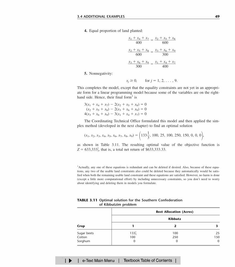
The Coordinating Technical Office formulated this model and then applied the sim-plex method (developed in the next chapter) to find an optimal solution

(x1, x2, x3, x4, x5, x6, x7, x8, x9) � �133�13

�, 100, 25, 100, 250, 150, 0, 0, 0�,

as shown in Table 3.11. The resulting optimal value of the objective function is Z � 633,333�

13

�, that is, a total net return of $633,333.33.


TABLE 3.11 Optimal solution for the Southern Confederation of Kibbutzim problem

Best Allocation (Acres)

Kibbutz

Crop 1 2 3

Sugar beets 133�13

� 100 25Cotton 100 250 150Sorghum 0 0 0

1Actually, any one of these equations is redundant and can be deleted if desired. Also, because of these equa-tions, any two of the usable land constraints also could be deleted because they automatically would be satis-fied when both the remaining usable land constraint and these equations are satisfied. However, no harm is done(except a little more computational effort) by including unnecessary constraints, so you don’t need to worryabout identifying and deleting them in models you formulate.

Controlling Air Pollution

The NORI & LEETS CO., one of the major producers of steel in its part of the world, islocated in the city of Steeltown and is the only large employer there. Steeltown has grownand prospered along with the company, which now employs nearly 50,000 residents. There-fore, the attitude of the townspeople always has been, “What’s good for Nori & Leets isgood for the town.” However, this attitude is now changing; uncontrolled air pollutionfrom the company’s furnaces is ruining the appearance of the city and endangering thehealth of its residents.

A recent stockholders’ revolt resulted in the election of a new enlightened board ofdirectors for the company. These directors are determined to follow socially responsiblepolicies, and they have been discussing with Steeltown city officials and citizens’ groupswhat to do about the air pollution problem. Together they have worked out stringent airquality standards for the Steeltown airshed.

The three main types of pollutants in this airshed are particulate matter, sulfur ox-ides, and hydrocarbons. The new standards require that the company reduce its annualemission of these pollutants by the amounts shown in Table 3.12. The board of directorshas instructed management to have the engineering staff determine how to achieve thesereductions in the most economical way.

The steelworks has two primary sources of pollution, namely, the blast furnaces formaking pig iron and the open-hearth furnaces for changing iron into steel. In both casesthe engineers have decided that the most effective types of abatement methods are (1) in-creasing the height of the smokestacks,1 (2) using filter devices (including gas traps) inthe smokestacks, and (3) including cleaner, high-grade materials among the fuels for thefurnaces. Each of these methods has a technological limit on how heavily it can be used(e.g., a maximum feasible increase in the height of the smokestacks), but there also isconsiderable flexibility for using the method at a fraction of its technological limit.

Table 3.13 shows how much emission (in millions of pounds per year) can be elim-inated from each type of furnace by fully using any abatement method to its technologi-cal limit. For purposes of analysis, it is assumed that each method also can be used lessfully to achieve any fraction of the emission-rate reductions shown in this table. Further-more, the fractions can be different for blast furnaces and for open-hearth furnaces. Foreither type of furnace, the emission reduction achieved by each method is not substan-tially affected by whether the other methods also are used.


1Subsequent to this study, this particular abatement method has become a controversial one. Because its effectis to reduce ground-level pollution by spreading emissions over a greater distance, environmental groups con-tend that this creates more acid rain by keeping sulfur oxides in the air longer. Consequently, the U.S. Envi-ronmental Protection Agency adopted new rules in 1985 to remove incentives for using tall smokestacks.

TABLE 3.12 Clean air standards for the Nori & Leets Co.

Required Reduction in Annual Emission RatePollutant (Million Pounds)

Particulates 60Sulfur oxides 150Hydrocarbons 125

After these data were developed, it became clear that no single method by itself couldachieve all the required reductions. On the other hand, combining all three methods at fullcapacity on both types of furnaces (which would be prohibitively expensive if the com-pany’s products are to remain competitively priced) is much more than adequate. There-fore, the engineers concluded that they would have to use some combination of the meth-ods, perhaps with fractional capacities, based upon the relative costs. Furthermore, becauseof the differences between the blast and the open-hearth furnaces, the two types probablyshould not use the same combination.

An analysis was conducted to estimate the total annual cost that would be incurredby each abatement method. A method’s annual cost includes increased operating and main-tenance expenses as well as reduced revenue due to any loss in the efficiency of the pro-duction process caused by using the method. The other major cost is the start-up cost (theinitial capital outlay) required to install the method. To make this one-time cost com-mensurable with the ongoing annual costs, the time value of money was used to calcu-late the annual expenditure (over the expected life of the method) that would be equiva-lent in value to this start-up cost.

This analysis led to the total annual cost estimates (in millions of dollars) given inTable 3.14 for using the methods at their full abatement capacities. It also was determinedthat the cost of a method being used at a lower level is roughly proportional to the frac-tion of the abatement capacity given in Table 3.13 that is achieved. Thus, for any givenfraction achieved, the total annual cost would be roughly that fraction of the correspond-ing quantity in Table 3.14.

The stage now was set to develop the general framework of the company’s plan forpollution abatement. This plan specifies which types of abatement methods will be usedand at what fractions of their abatement capacities for (1) the blast furnaces and (2) theopen-hearth furnaces. Because of the combinatorial nature of the problem of finding a


TABLE 3.13 Reduction in emission rate (in millions of pounds per year) from themaximum feasible use of an abatement method for Nori & Leets Co.

Taller Smokestacks Filters Better Fuels

Blast Open-Hearth Blast Open-Hearth Blast Open-HearthPollutant Furnaces Furnaces Furnaces Furnaces Furnaces Furnaces

Particulates 12 9 25 20 17 13Sulfur oxides 35 42 18 31 56 49Hydrocarbons 37 53 28 24 29 20

TABLE 3.14 Total annual cost from the maximum feasible use of an abatementmethod for Nori & Leets Co. ($ millions)

Abatement Method Blast Furnaces Open-Hearth Furnaces

Taller smokestacks 8 10Filters 7 6Better fuels 11 9

plan that satisfies the requirements with the smallest possible cost, an OR team was formedto solve the problem. The team adopted a linear programming approach, formulating themodel summarized next.

Formulation as a Linear Programming Problem. This problem has six decisionvariables xj, j � 1, 2, . . . , 6, each representing the use of one of the three abatementmethods for one of the two types of furnaces, expressed as a fraction of the abatementcapacity (so xj cannot exceed 1). The ordering of these variables is shown in Table 3.15.Because the objective is to minimize total cost while satisfying the emission reduction re-quirements, the data in Tables 3.12, 3.13, and 3.14 yield the following model:

Minimize Z � 8x1 � 10x2 � 7x3 � 6x4 � 11x5 � 9x6,


1. Emission reduction:

12x1 � 9x2 � 25x3 � 20x4 � 17x5 � 13x6 � 6035x1 � 42x2 � 18x3 � 31x4 � 56x5 � 49x6 � 15037x1 � 53x2 � 28x3 � 24x4 � 29x5 � 20x6 � 125

2. Technological limit:

xj � 1, for j � 1, 2, . . . , 6

3. Nonnegativity:

xj � 0, for j � 1, 2, . . . , 6.

The OR team used this model1 to find a minimum-cost plan

(x1, x2, x3, x4, x5, x6) � (1, 0.623, 0.343, 1, 0.048, 1),

with Z � 32.16 (total annual cost of $32.16 million). Sensitivity analysis then was con-ducted to explore the effect of making possible adjustments in the air standards given inTable 3.12, as well as to check on the effect of any inaccuracies in the cost data given inTable 3.14. (This story is continued in Case 6.1 at the end of Chap. 6.) Next came de-tailed planning and managerial review. Soon after, this program for controlling air pollu-tion was fully implemented by the company, and the citizens of Steeltown breathed deep(cleaner) sighs of relief.


1An equivalent formulation can express each decision variable in natural units for its abatement method; for ex-ample, x1 and x2 could represent the number of feet that the heights of the smokestacks are increased.

TABLE 3.15 Decision variables (fraction of the maximum feasible use of anabatement method) for Nori & Leets Co.

Abatement Method Blast Furnaces Open-Hearth Furnaces

Taller smokestacks x1 x2

Filters x3 x4

Better fuels x5 x6

Reclaiming Solid Wastes

The SAVE-IT COMPANY operates a reclamation center that collects four types of solidwaste materials and treats them so that they can be amalgamated into a salable product.(Treating and amalgamating are separate processes.) Three different grades of this prod-uct can be made (see the first column of Table 3.16), depending upon the mix of the ma-terials used. Although there is some flexibility in the mix for each grade, quality standardsmay specify the minimum or maximum amount allowed for the proportion of a materialin the product grade. (This proportion is the weight of the material expressed as a per-centage of the total weight for the product grade.) For each of the two higher grades, afixed percentage is specified for one of the materials. These specifications are given inTable 3.16 along with the cost of amalgamation and the selling price for each grade.

The reclamation center collects its solid waste materials from regular sources and sois normally able to maintain a steady rate for treating them. Table 3.17 gives the quanti-ties available for collection and treatment each week, as well as the cost of treatment, foreach type of material.

The Save-It Co. is solely owned by Green Earth, an organization devoted to dealingwith environmental issues, so Save-It’s profits are used to help support Green Earth’s ac-tivities. Green Earth has raised contributions and grants, amounting to $30,000 per week,to be used exclusively to cover the entire treatment cost for the solid waste materials. Theboard of directors of Green Earth has instructed the management of Save-It to divide thismoney among the materials in such a way that at least half of the amount available ofeach material is actually collected and treated. These additional restrictions are listed inTable 3.17.

Within the restrictions specified in Tables 3.16 and 3.17, management wants to de-termine the amount of each product grade to produce and the exact mix of materials tobe used for each grade. The objective is to maximize the net weekly profit (total sales in-come minus total amalgamation cost), exclusive of the fixed treatment cost of $30,000 perweek that is being covered by gifts and grants.

Formulation as a Linear Programming Problem. Before attempting to constructa linear programming model, we must give careful consideration to the proper definitionof the decision variables. Although this definition is often obvious, it sometimes becomes


TABLE 3.16 Product data for Save-It Co.

Amalgamation Selling PriceGrade Specification Cost per Pound ($) per Pound ($)

Material 1: Not more than 30% of totalMaterial 2: Not less than 40% of total

A 3.00 8.50Material 3: Not more than 50% of totalMaterial 4: Exactly 20% of total

Material 1: Not more than 50% of totalB Material 2: Not less than 10% of total 2.50 7.00

Material 4: Exactly 10% of total

C Material 1: Not more than 70% of total 2.00 5.50

the crux of the entire formulation. After clearly identifying what information is really de-sired and the most convenient form for conveying this information by means of decisionvariables, we can develop the objective function and the constraints on the values of thesedecision variables.

In this particular problem, the decisions to be made are well defined, but the appro-priate means of conveying this information may require some thought. (Try it and see ifyou first obtain the following inappropriate choice of decision variables.)

Because one set of decisions is the amount of each product grade to produce, it wouldseem natural to define one set of decision variables accordingly. Proceeding tentativelyalong this line, we define

yi � number of pounds of product grade i produced per week (i � A, B, C).

The other set of decisions is the mix of materials for each product grade. This mix is iden-tified by the proportion of each material in the product grade, which would suggest defin-ing the other set of decision variables as

zij � proportion of material j in product grade i (i � A, B, C; j � 1, 2, 3, 4).

However, Table 3.17 gives both the treatment cost and the availability of the materials byquantity (pounds) rather than proportion, so it is this quantity information that needs tobe recorded in some of the constraints. For material j ( j � 1, 2, 3, 4),

Number of pounds of material j used per week � zAjyA � zBjyB � zCjyC.

For example, since Table 3.17 indicates that 3,000 pounds of material 1 is available perweek, one constraint in the model would be

zA1yA � zB1yB � zC1yC � 3,000.

Unfortunately, this is not a legitimate linear programming constraint. The expression onthe left-hand side is not a linear function because it involves products of variables. There-fore, a linear programming model cannot be constructed with these decision variables.

Fortunately, there is another way of defining the decision variables that will fit thelinear programming format. (Do you see how to do it?) It is accomplished by merely re-placing each product of the old decision variables by a single variable! In other words,define

xij � zijyi (for i � A, B, C; j � 1, 2, 3, 4) xij � number of pounds of material j allocated to product grade i per week,


TABLE 3.17 Solid waste materials data for the Save-It Co.

Pounds per Treatment CostMaterial Week Available per Pound ($) Additional Restrictions

1 3,000 3.00 1. For each material, at least half of the2 2,000 6.00 pounds per week available should be3 4,000 4.00 collected and treated.4 1,000 5.00 2. $30,000 per week should be used to

treat these materials.

and then we let the xij be the decision variables. Combining the xij in different ways yieldsthe following quantities needed in the model (for i � A, B, C; j � 1, 2, 3, 4).

xi1 � xi2 � xi3 � xi4 � number of pounds of product grade i produced per week.xAj � xBj � xCj � number of pounds of material j used per week.

� proportion of material j in product grade i.

The fact that this last expression is a nonlinear function does not cause a complica-tion. For example, consider the first specification for product grade A in Table 3.16 (theproportion of material 1 should not exceed 30 percent). This restriction gives the nonlin-ear constraint

� 0.3.

However, multiplying through both sides of this inequality by the denominator yields anequivalent constraint

xA1 � 0.3(xA1 � xA2 � xA3 � xA4),

so

0.7xA1 � 0.3xA2 � 0.3xA3 � 0.3xA4 � 0,

which is a legitimate linear programming constraint.With this adjustment, the three quantities given above lead directly to all the functional

constraints of the model. The objective function is based on management’s objective of max-imizing net weekly profit (total sales income minus total amalgamation cost) from the threeproduct grades. Thus, for each product grade, the profit per pound is obtained by subtract-ing the amalgamation cost given in the third column of Table 3.16 from the selling price inthe fourth column. These differences provide the coefficients for the objective function.

Therefore, the complete linear programming model is

Maximize Z � 5.5(xA1 � xA2 � xA3 � xA4) � 4.5(xB1 � xB2 � xB3 � xB4)� 3.5(xC1 � xC2 � xC3 � xC4),


1. Mixture specifications (second column of Table 3.16):

xA1 � 0.3(xA1 � xA2 � xA3 � xA4) (grade A, material 1)



xA4 � 0.2(xA1 � xA2 � xA3 � xA4) (grade A, material 4).

xB1 � 0.5(xB1 � xB2 � xB3 � xB4) (grade B, material 1)

xB2 � 0.1(xB1 � xB2 � xB3 � xB4) (grade B, material 2)

xB4 � 0.1(xB1 � xB2 � xB3 � xB4) (grade B, material 4).

xC1 � 0.7(xC1 � xC2 � xC3 � xC4) (grade C, material 1).

xA1��xA1 � xA2 � xA3 � xA4

xij��xi1 � xi2 � xi3 � xi4


2. Availability of materials (second column of Table 3.17):

xA1 � xB1 � xC1 � 3,000 (material 1)

xA2 � xB2 � xC2 � 2,000 (material 2)

xA3 � xB3 � xC3 � 4,000 (material 3)

xA4 � xB4 � xC4 � 1,000 (material 4).

3. Restrictions on amounts treated (right side of Table 3.17):

xA1 � xB1 � xC1 � 1,500 (material 1)

xA2 � xB2 � xC2 � 1,000 (material 2)

xA3 � xB3 � xC3 � 2,000 (material 3)

xA4 � xB4 � xC4 � 500 (material 4).

4. Restriction on treatment cost (right side of Table 3.17):

3(xA1 � xB1 � xC1) � 6(xA2 � xB2 � xC2) � 4(xA3 � xB3 � xC3)

� 5(xA4 � xB4 � xC4) � 30,000.

5. Nonnegativity constraints:

xA1 � 0, xA2 � 0, . . . , xC4 � 0.

This formulation completes the model, except that the constraints for the mixturespecifications need to be rewritten in the proper form for a linear programming model bybringing all variables to the left-hand side and combining terms, as follows:

Mixture specifications:

0.7xA1 � 0.3xA2 � 0.3xA3 � 0.3xA4 � 0 (grade A, material 1)

�0.4xA1 � 0.6xA2 � 0.4xA3 � 0.4xA4 � 0 (grade A, material 2)

�0.5xA1 � 0.5xA2 � 0.5xA3 � 0.5xA4 � 0 (grade A, material 3)

�0.2xA1 � 0.2xA2 � 0.2xA3 � 0.8xA4 � 0 (grade A, material 4).

0.5xB1 � 0.5xB2 � 0.5xB3 � 0.5xB4 � 0 (grade B, material 1)

�0.1xB1 � 0.9xB2 � 0.1xB3 � 0.1xB4 � 0 (grade B, material 2)

�0.1xB1 � 0.1xB2 � 0.1xB3 � 0.9xB4 � 0 (grade B, material 4).

0.3xC1 � 0.7xC2 � 0.7xC3 � 0.7xC4 � 0 (grade C, material 1).

An optimal solution for this model is shown in Table 3.18, and then these xij valuesare used to calculate the other quantities of interest given in the table. The resulting op-timal value of the objective function is Z � 35,108.90 (a total weekly profit of $35,108.90).

The Save-It Co. problem is an example of a blending problem. The objective fora blending problem is to find the best blend of ingredients into final products to meetcertain specifications. Some of the earliest applications of linear programming werefor gasoline blending, where petroleum ingredients were blended to obtain variousgrades of gasoline. The award-winning OR study at Texaco discussed at the end of


Sec. 2.5 dealt with gasoline blending (although Texaco used a nonlinear programmingmodel). Other blending problems involve such final products as steel, fertilizer, andanimal feed.

Personnel Scheduling

UNION AIRWAYS is adding more flights to and from its hub airport, and so it needs tohire additional customer service agents. However, it is not clear just how many moreshould be hired. Management recognizes the need for cost control while also consistentlyproviding a satisfactory level of service to customers. Therefore, an OR team is studyinghow to schedule the agents to provide satisfactory service with the smallest personnel cost.

Based on the new schedule of flights, an analysis has been made of the minimumnumber of customer service agents that need to be on duty at different times of the dayto provide a satisfactory level of service. The rightmost column of Table 3.19 shows thenumber of agents needed for the time periods given in the first column. The other entries


TABLE 3.18 Optimal solution for the Save-It Co. problem

Pounds Used per Week

MaterialNumber of Pounds

Grade 1 2 3 4 Produced per Week

A 412.3 859.6 447.4 429.8 2149(19.2%) (40%) (20.8%) (20%)

B 2587.7 517.5 1552.6 517.5 5175(50%) (10%) (30%) (10%)

C 0 0 0 0 0

Total 3000 1377 2000 947

TABLE 3.19 Data for the Union Airways personnel scheduling problem

Time Periods Covered

ShiftMinimum Number of

Time Period 1 2 3 4 5 Agents Needed

6:00 A.M. to 8:00 A.M. ✔ 488:00 A.M. to 10:00 A.M. ✔ ✔ 7910:00 A.M. to noon ✔ ✔ 65Noon to 2:00 P.M. ✔ ✔ ✔ 872:00 P.M. to 4:00 P.M. ✔ ✔ 644:00 P.M. to 6:00 P.M. ✔ ✔ 736:00 P.M. to 8:00 P.M. ✔ ✔ 828:00 P.M. to 10:00 P.M. ✔ 4310:00 P.M. to midnight ✔ ✔ 52Midnight to 6:00 A.M. ✔ 15

Daily cost per agent $170 $160 $175 $180 $195

in this table reflect one of the provisions in the company’s current contract with the unionthat represents the customer service agents. The provision is that each agent work an 8-hour shift 5 days per week, and the authorized shifts are

Shift 1: 6:00 A.M. to 2:00 P.M.Shift 2: 8:00 A.M. to 4:00 P.M.Shift 3: Noon to 8:00 P.M.Shift 4: 4:00 P.M. to midnightShift 5: 10:00 P.M. to 6:00 A.M.

Checkmarks in the main body of Table 3.19 show the hours covered by the respectiveshifts. Because some shifts are less desirable than others, the wages specified in the con-tract differ by shift. For each shift, the daily compensation (including benefits) for eachagent is shown in the bottom row. The problem is to determine how many agents shouldbe assigned to the respective shifts each day to minimize the total personnel cost for agents,based on this bottom row, while meeting (or surpassing) the service requirements givenin the rightmost column.

Formulation as a Linear Programming Problem. Linear programming problemsalways involve finding the best mix of activity levels. The key to formulating this partic-ular problem is to recognize the nature of the activities.

Activities correspond to shifts, where the level of each activity is the number of agentsassigned to that shift. Thus, this problem involves finding the best mix of shift sizes. Since thedecision variables always are the levels of the activities, the five decision variables here are

xj � number of agents assigned to shift j, for j � 1, 2, 3, 4, 5.

The main restrictions on the values of these decision variables are that the number ofagents working during each time period must satisfy the minimum requirement given inthe rightmost column of Table 3.19. For example, for 2:00 P.M. to 4:00 P.M., the total num-ber of agents assigned to the shifts that cover this time period (shifts 2 and 3) must be atleast 64, so

x2 � x3 � 64

is the functional constraint for this time period.Because the objective is to minimize the total cost of the agents assigned to the five

shifts, the coefficients in the objective function are given by the last row of Table 3.19.Therefore, the complete linear programming model is

Minimize Z � 170x1 � 160x2 � 175x3 � 180x4 � 195x5,

subject to

x1 � 48 (6–8 A.M.)x1 � x2 � 79 (8–10 A.M.)x1 � x2 � 65 (10 A.M. to noon)x1 � x2 � x3 � 87 (Noon–2 P.M.)

x2 � x3 � 64 (2–4 P.M.)x3 � x4 � 73 (4–6 P.M.)


x3 � x4 � 82 (6–8 P.M.)x4 � 43 (8–10 P.M.)x4 � x5 � 52 (10 P.M.–midnight)

x5 � 15 (Midnight–6 A.M.)

and

xj � 0, for j � 1, 2, 3, 4, 5.

With a keen eye, you might have noticed that the third constraint, x1 � x2 � 65, ac-tually is not necessary because the second constraint, x1 � x2 � 79, ensures that x1 � x2

will be larger than 65. Thus, x1 � x2 � 65 is a redundant constraint that can be deleted.Similarly, the sixth constraint, x3 � x4 � 73, also is a redundant constraint because theseventh constraint is x3 � x4 � 82. (In fact, three of the nonnegativity constraints—x1 � 0,x4 � 0, x5 � 0—also are redundant constraints because of the first, eighth, and tenth func-tional constraints: x1 � 48, x4 � 43, and x5 � 15. However, no computational advantageis gained by deleting these three nonnegativity constraints.)

The optimal solution for this model is (x1, x2, x3, x4, x5) � (48, 31, 39, 43, 15). Thisyields Z � 30,610, that is, a total daily personnel cost of $30,610.

This problem is an example where the divisibility assumption of linear programmingactually is not satisfied. The number of agents assigned to each shift needs to be an inte-ger. Strictly speaking, the model should have an additional constraint for each decisionvariable specifying that the variable must have an integer value. Adding these constraintswould convert the linear programming model to an integer programming model (the topicof Chap. 12).

Without these constraints, the optimal solution given above turned out to have inte-ger values anyway, so no harm was done by not including the constraints. (The form ofthe functional constraints made this outcome a likely one.) If some of the variables hadturned out to be noninteger, the easiest approach would have been to round up to integervalues. (Rounding up is feasible for this example because all the functional constraintsare in � form with nonnegative coefficients.) Rounding up does not ensure obtaining anoptimal solution for the integer programming model, but the error introduced by round-ing up such large numbers would be negligible for most practical situations. Alternatively,integer programming techniques described in Chap. 12 could be used to solve exactly foran optimal solution with integer values.

Section 3.5 includes a case study of how United Airlines used linear programming todevelop a personnel scheduling system on a vastly larger scale than this example.

Distributing Goods through a Distribution Network

The Problem. The DISTRIBUTION UNLIMITED CO. will be producing the samenew product at two different factories, and then the product must be shipped to two ware-houses, where either factory can supply either warehouse. The distribution network avail-able for shipping this product is shown in Fig. 3.13, where F1 and F2 are the two facto-ries, W1 and W2 are the two warehouses, and DC is a distribution center. The amountsto be shipped from F1 and F2 are shown to their left, and the amounts to be received atW1 and W2 are shown to their right. Each arrow represents a feasible shipping lane. Thus,F1 can ship directly to W1 and has three possible routes (F1 � DC � W2, F1 � F2 �


DC � W2, and F1 � W1 � W2) for shipping to W2. Factory F2 has just one route toW2 (F2 � DC � W2) and one to W1 (F2 � DC � W2 � W1). The cost per unitshipped through each shipping lane is shown next to the arrow. Also shown next to F1 �F2 and DC � W2 are the maximum amounts that can be shipped through these lanes.The other lanes have sufficient shipping capacity to handle everything these factories cansend.

The decision to be made concerns how much to ship through each shipping lane. Theobjective is to minimize the total shipping cost.

Formulation as a Linear Programming Problem. With seven shipping lanes, weneed seven decision variables (xF1-F2, xF1-DC, xF1-W1, xF2-DC, xDC-W2, xW1-W2, xW2-W1) torepresent the amounts shipped through the respective lanes.

There are several restrictions on the values of these variables. In addition to the usualnonnegativity constraints, there are two upper-bound constraints, xF1-F2 � 10 and xDC-W2 � 80, imposed by the limited shipping capacities for the two lanes, F1 � F2 andDC � W2. All the other restrictions arise from five net flow constraints, one for each ofthe five locations. These constraints have the following form.

Net flow constraint for each location:

Amount shipped out � amount shipped in � required amount.

As indicated in Fig. 3.13, these required amounts are 50 for F1, 40 for F2, �30 for W1,and �60 for W2.


F1

F2

DC

W1

W2

50 unitsproduced

$900/unit 30 unitsneeded

$400/unit

$200/unit

40 unitsproduced

$100/unit

80 units max.

$200/unit $300/unit

$300

/unit

60 unitsneeded

10 units max.

FIGURE 3.13The distribution network forDistribution Unlimited Co.

What is the required amount for DC? All the units produced at the factories are ulti-mately needed at the warehouses, so any units shipped from the factories to the distribu-tion center should be forwarded to the warehouses. Therefore, the total amount shippedfrom the distribution center to the warehouses should equal the total amount shipped fromthe factories to the distribution center. In other words, the difference of these two ship-ping amounts (the required amount for the net flow constraint) should be zero.

Since the objective is to minimize the total shipping cost, the coefficients for the ob-jective function come directly from the unit shipping costs given in Fig. 3.13. Therefore,by using money units of hundreds of dollars in this objective function, the complete lin-ear programming model is

Minimize Z � 2xF1-F2 � 4xF1-DC � 9xF1-W1 � 3xF2-DC � xDC-W2

� 3xW1-W2 � 2xW2-W1,


1. Net flow constraints:

3.5 SOME CASE STUDIES 61

To give you a better perspective about the great impact linear programming can have, wenow present three case studies of real applications. Each of these is a classic application,initiated in the early 1980s, that has come to be regarded as a standard of excellence forfuture applications of linear programming. The first one will bear some strong similari-ties to the Wyndor Glass Co. problem, but on a realistic scale. Similarly, the second and

3.5 SOME CASE STUDIES

�xF1-F2 � xF1-DC � xF1-W1 � 50 (factory 1)�xF1-F2 � xF2-DC � 40 (factory 2)

� xF1-DC � xF2-DC � xDC-W2 � 0 (distribution center)

� xF1-W1 � xW1-W2 � xW2-W1 � �30 (warehouse 1)� xDC-W2 � xW1-W2 � xW2-W1 � �60 (warehouse 2)

2. Upper-bound constraints:

xF1-F2 � 10, xDC-W2 � 80

3. Nonnegativity constraints:

xF1-F2 � 0, xF1-DC � 0, xF1-W1 � 0, xF2-DC � 0, xDC-W2 � 0,xW1-W2 � 0, xW2-W1 � 0.

You will see this problem again in Sec. 9.6, where we focus on linear programmingproblems of this type (called the minimum cost flow problem). In Sec. 9.7, we will solvefor its optimal solution:

xF1-F2 � 0, xF1-DC � 40, xF1-W1 � 10, xF2-DC � 40, xDC-W2 � 80,xW1-W2 � 0, xW2-W1 � 20.

The resulting total shipping cost is $49,000.You also will see a case study involving a much larger problem of this same type at

the end of the next section.

third are realistic versions of the last two examples presented in the preceding section (theUnion Airways and Distribution Unlimited examples).

Choosing the Product Mix at Ponderosa Industrial1

Until its sale in 1988, PONDEROSA INDUSTRIAL was a plywood manufacturer basedin Anhuac, Chihuahua, that supplied 25 percent of the plywood in Mexico. Like any ply-wood manufacturer, Ponderosa’s many products were differentiated by thickness and bythe quality of the wood. The plywood market in Mexico is competitive, so the market es-tablishes the prices of the products. The prices can fluctuate considerably from month tomonth, and there may be great differences between the products in their price movementsfrom even one month to the next. As a result, each product’s contribution to Ponderosa’stotal profit was continually varying, and in different ways for different products.

Because of its pronounced effect on profits, a critical issue facing management wasthe choice of product mix—how much to produce of each product—on a monthly basis.This choice was a very complex one, since it had to take into account the current amountsavailable of various resources needed to produce the products. The most important re-sources were logs in four quality categories and production capacities for both the press-ing operation and the polishing operation.

Beginning in 1980, linear programming was used on a monthly basis to guide theproduct-mix decision. The linear programming model had an objective of maximizing thetotal profit from all products. The model’s constraints included the various resource con-straints as well as other relevant restrictions such as the minimum amount of a productthat must be provided to regular customers and the maximum amount that can be sold.(To aid planning for the procurement of raw materials, the model also considered the im-pact of the product-mix decision for the upcoming month on production in the followingmonth.) The model had 90 decision variables and 45 functional constraints.

This model was used each month to find the product mix for the upcoming monththat would be optimal if the estimated values of the various parameters of the model proveto be accurate. However, since some of the parameter values could change quickly (e.g.,the unit profits of the products), sensitivity analysis was done to determine the effect ifthe estimated values turned out to be inaccurate. The results indicated when adjustmentsin the product mix should be made (if time permitted) as unanticipated market changesoccurred that affected the price (and so the unit profit) of certain products.

One key decision each month concerned the number of logs in each of the four qual-ity categories to purchase. The amounts available for the upcoming month’s productionactually were parameters of the model. Therefore, after the purchase decision was madeand then the corresponding optimal product mix was determined, postoptimality analysiswas conducted to investigate the effect of adjusting the purchase decision. For example,it is very easy with linear programming to check what the impact on total profit wouldbe if a quick purchase were to be made of additional logs in a certain quality category toenable increasing production for the upcoming month.

Ponderosa’s linear programming system was interactive, so management received animmediate response to its “what-if questions” about the impact of encountering parame-


1A. Roy, E. E. DeFalomir, and L. Lasdon: “An Optimization-Based Decision Support System for a Product MixProblem,” Interfaces, 12(2):26–33, April 1982.

ter values that differ from those in the original model. What if a quick purchase of logsof a certain kind were made? What if product prices were to fluctuate in a certain way?A variety of such scenarios can be investigated. Management effectively used this powerto reach better decisions than the “optimal” product mix from the original model.

The impact of linear programming at Ponderosa was reported to be “tremendous.” Itled to a dramatic shift in the types of plywood products emphasized by the company. Theimproved product-mix decisions were credited with increasing the overall profitability ofthe company by 20 percent. Other contributions of linear programming included betterutilization of raw material, capital equipment, and personnel.

Two factors helped make this application of linear programming so successful. Onefactor is that a natural language financial planning system was interfaced with the codesfor finding an optimal solution for the linear programming model. Using natural languagerather than mathematical symbols to display the components of the linear programmingmodel and its output made the process understandable and meaningful for the managersmaking the product-mix decisions. Reporting to management in the language of managersis necessary for the successful application of linear programming.

The other factor was that the linear programming system used was interactive. Asmentioned earlier, after an optimal solution was obtained for one version of the model,this feature enabled managers to ask a variety of “what-if” questions and receive imme-diate responses. Better decisions frequently were reached by exploring other plausible sce-narios, and this process also gave managers more confidence that their decision wouldperform well under most foreseeable circumstances.

In any application, this ability to respond quickly to management’s needs and queriesthrough postoptimality analysis (whether interactive or not) is a vital part of a linear pro-gramming study.

Personnel Scheduling at United Airlines1

Despite unprecedented industry competition in 1983 and 1984, UNITED AIRLINES man-aged to achieve substantial growth with service to 48 new airports. In 1984, it became theonly airline with service to cities in all 50 states. Its 1984 operating profit reached $564million, with revenues of $6.2 billion, an increase of 6 percent over 1983, while costsgrew by less than 2 percent.

Cost control is essential to competing successfully in the airline industry. In 1982,upper management of United Airlines initiated an OR study of its personnel schedulingas part of the cost control measures associated with the airline’s 1983–1984 expansion.The goal was to schedule personnel at the airline’s reservations offices and airports so asto minimize the cost of providing the necessary service to customers.

At the time, United Airlines employed over 4,000 reservations sales representativesand support personnel at its 11 reservations offices and about 1,000 customer serviceagents at its 10 largest airports. Some were part-time, working shifts from 2 to 8 hours;most were full-time, working 8- or 10-hour-shifts. Shifts start at several different times.Each reservations office was open (by telephone) 24 hours a day, as was each of the ma-jor airports. However, the number of employees needed at each location to provide the re-


1T. J. Holloran and J. E. Bryn, “United Airlines Station Manpower Planning System,” Interfaces, 16(1): 39–50,Jan.–Feb. 1986.

quired level of service varied greatly during the 24-hour day, and might fluctuate consid-erably from one half-hour to the next.

Trying to design the work schedules for all the employees at a given location to meetthese service requirements most efficiently is a nightmare of combinatorial considerations.Once an employee begins working, he or she will be there continuously for the entire shift(2 to 10 hours, depending on the employee), except for either a meal break or short restbreaks every 2 hours. Given the minimum number of employees needed on duty for eachhalf-hour interval over a 24-hour day (where these requirements change from day to dayover a 7-day week), how many employees of each shift length should begin work at whatstart time over each 24-hour day of a 7-day week? Fortunately, linear programming thriveson such combinatorial nightmares.

Actually, several OR techniques described in this book were used in the computerizedplanning system developed to attack this problem. Both forecasting (Chap. 20) and queu-ing theory (Chaps. 17 and 18) were used to determine the minimum number of employeesneeded on duty for each half-hour interval. Integer programming (Chap. 12) was used todetermine the times of day at which shifts would be allowed to start. However, the core ofthe planning system was linear programming, which did all the actual scheduling to pro-vide the needed service with the smallest possible labor cost. A complete work schedulewas developed for the first full week of a month, and then it was reused for the remainderof the month. This process was repeated each month to reflect changing conditions.

Although the details about the linear programming model have not been published,it is clear that the basic approach used is the one illustrated by the Union Airways exam-ple of personnel scheduling in Sec. 3.4. The objective function being minimized repre-sents the total personnel cost for the location being scheduled. The main functional con-straints require that the number of employees on duty during each time period will notfall below minimum acceptable levels.

However, the Union Airways example has only five decision variables. By contrast,the United Airlines model for some locations has over 20,000 decision variables! The dif-ference is that a real application must consider myriad important details that can be ig-nored in a textbook example. For example, the United Airlines model takes into accountsuch things as the meal and break assignment times for each employee scheduled, differ-ences in shift lengths for different employees, and days off over a weekly schedule, amongother scheduling details.

This application of linear programming was reported to have had “an overwhelmingimpact not only on United management and members of the manpower planning group, butalso for many who had never before heard of management science (OR) or mathematicalmodeling.” It earned rave reviews from upper management, operating managers, and af-fected employees alike. For example, one manager described the scheduling system as

Magical, . . . just as the [customer] lines begin to build, someone shows up for work, andjust as you begin to think you’re overstaffed, people start going home.1

In more tangible terms, this application was credited with saving United Airlines morethan $6 million annually in just direct salary and benefit costs. Other benefits includedimproved customer service and reduced need for support staff.


1Holloran and Bryn, “United Airlines Station Manpower Planning System,” p. 49.

After some updating in the early 1990s, the system is providing similar benefitstoday.

One factor that helped make this application of linear programming so successful was“the support of operational managers and their staffs.” This was a lesson learned by ex-perience, because the OR team initially failed to establish a good line of communicationwith the operating managers, who then resisted the team’s initial recommendations. Theteam leaders described their mistake as follows:

The cardinal rule for earning the trust and respect of operating managers and supportstaffs—”getting them involved in the development process”—had been violated.1

The team then worked much more closely with the operating managers—with outstand-ing results.

Planning Supply, Distribution, and Marketing at Citgo Petroleum Corporation2

CITGO PETROLEUM CORPORATION specializes in refining and marketing petroleum.In the mid-1980s, it had annual sales of several billion dollars, ranking it among the 150largest industrial companies in the United States.

After several years of financial losses, Citgo was acquired in 1983 by Southland Cor-poration, the owner of the 7-Eleven convenience store chain (whose sales include 2 bil-lion gallons of quality motor fuels annually). To turn Citgo’s financial losses around, South-land created a task force composed of Southland personnel, Citgo personnel, and outsideconsultants. An eminent OR consultant was appointed director of the task force to reportdirectly to both the president of Citgo and the chairman of the board of Southland.

During 1984 and 1985, this task force applied various OR techniques (as well as in-formation systems technologies) throughout the corporation. It was reported that these ORapplications “have changed the way Citgo does business and resulted in approximately$70 million per year profit improvement.”3

The two most important applications were both linear programming systems that pro-vided management with powerful planning support. One, called the refinery LP system,led to great improvements in refinery yield, substantial reductions in the cost of labor, andother important cost savings. This system contributed approximately $50 million to profitimprovement in 1985. (See the end of Sec. 2.4 for discussion of the key role that modelvalidation played in the development of this system.)

However, we will focus here on the other linear programming system, called the sup-ply, distribution, and marketing modeling system (or just the SDM system), that Citgo iscontinuing to use. The SDM system is particularly interesting because it is based on aspecial kind of linear programming model that uses networks, just like the model for theDistribution Unlimited example presented at the end of Sec. 3.4. The model for the SDMsystem provides a representation of Citgo’s entire marketing and distribution network.

At the time the task force conducted its OR study, Citgo owned or leased 36 productstorage terminals which were supplied through five distribution center terminals via a dis-


1Ibid, p. 47.2See the references cited in footnote 2 on p. 10.3See p. 4 of the second reference cited in footnote 2 on p. 10.

tribution network of pipelines, tankers, and barges. Citgo also sold product from over 350exchange terminals that were shared with other petroleum marketers. To supply its cus-tomers, product might be acquired by Citgo from its refinery in Lake Charles, LA, or fromspot purchases on one of five major spot markets, product exchanges, and trades withother industry refiners. These product acquisition decisions were made daily. However,the time from such a decision until the product reached the intended customers could beas long as 11 weeks. Therefore, the linear programming model used an 11-week planninghorizon.

The SDM system is used to coordinate the supply, distribution, and marketing of eachof Citgo’s major products (originally four grades of motor fuel and No. 2 fuel oil) through-out the United States. Management uses the system to make decisions such as where tosell, what price to charge, where to buy or trade, how much to buy or trade, how muchto hold in inventory, and how much to ship by each mode of transportation. Linear pro-gramming guides these decisions and when to implement them so as to minimize totalcost or maximize total profit. The SDM system also is used in “what-if” sessions, wheremanagement asks what-if questions about scenarios that differ from those assumed in theoriginal model.

The linear programming model in the SDM system has the same form as the modelfor the Distribution Unlimited example presented at the end of Sec. 3.4. In fact, both mod-els fit an important special kind of linear programming problem, called the minimum costflow problem, that will be discussed in Sec. 9.6. The main functional constraints for suchmodels are equality constraints, where each one prescribes what the net flow of goodsout of a specific location must be.

The Distribution Unlimited model has just seven decision variables and five equalityconstraints. By contrast, the Citgo model for each major product has about 15,000 deci-sion variables and 3,000 equality constraints!

At the end of Sec. 2.1, we described the important role that data collection and dataverification played in developing the Citgo models. With such huge models, a massiveamount of data must be gathered to determine all the parameter values. A state-of-the-artmanagement database system was developed for this purpose. Before using the data, apreloader program was used to check for data errors and inconsistencies. The importanceof doing so was brought forcefully home to the task force when, as mentioned in Sec. 2.1,the initial run of the preloader program generated a paper log of error messages an inchthick! It was clear that the data collection process needed to be thoroughly debugged tohelp ensure the validity of the models.

The SDM linear programming system has greatly improved the efficiency of Citgo’ssupply, distribution, and marketing operations, enabling a huge reduction in product in-ventory with no drop in service levels. During its first year, the value of petroleum prod-ucts held in inventory was reduced by $116.5 million. This huge reduction in capital tiedup in carrying inventory resulted in saving about $14 million annually in interest expensesfor borrowed capital, adding $14 million to Citgo’s annual profits. Improvements in co-ordination, pricing, and purchasing decisions have been estimated to add at least another$2.5 million to annual profits. Many indirect benefits also are attributed to this applica-tion of linear programming, including improved data, better pricing strategies, and elim-ination of unnecessary product terminals, as well as improved communication and coor-dination between supply, distribution, marketing, and refinery groups.


Some of the factors that contributed to the success of this OR study are the same asfor the two preceding case studies. Like Ponderosa Industrial, one factor was developingoutput reports in the language of managers to really meet their needs. These output re-ports are designed to be easy for managers to understand and use, and they address theissues that are important to management. Also like Ponderosa, another factor was enablingmanagement to respond quickly to the dynamics of the industry by using the linear pro-gramming system extensively in “what-if” sessions. As in so many applications of linearprogramming, postoptimality analysis proved more important than the initial optimal so-lution obtained for one version of the model.

Much as in the United Airlines application, another factor was the enthusiastic sup-port of operational managers during the development and implementation of this linearprogramming system.

However, the most important factor was the unlimited support provided to the taskforce by top management, ranging right up to the chief executive officer and the chair-man of the board of Citgo’s parent company, Southland Corporation. As mentioned ear-lier, the director of the task force (an eminent OR consultant) reported directly to both thepresident of Citgo and the chairman of the board of Southland. This backing by top man-agement included strong organizational and financial support.

The organizational support took a variety of forms. One example was the creationand staffing of the position of senior vice-president of operations coordination to evalu-ate and coordinate recommendations based on the models which spanned organizationalboundaries.

When discussing both this linear programming system and other OR applications im-plemented by the task force, team members described the financial support of top man-agement as follows:

The total cost of the systems implemented, $20 million to $30 million, was the greatestobstacle to this project. However, because of the information explosion in the petroleumindustry, top management realized that numerous information systems were essential togather, store, and analyze data. The incremental cost of adding management science (OR)technologies to these computers and systems was small, in fact very small in light of theenormous benefits they provided.1

3.6 DISPLAYING AND SOLVING LINEAR PROGRAMMING MODELS ON A SPREADSHEET 67

Spreadsheet software, such as Excel, is a popular tool for analyzing and solving small lin-ear programming problems. The main features of a linear programming model, includingall its parameters, can be easily entered onto a spreadsheet. However, spreadsheet soft-ware can do much more than just display data. If we include some additional informa-tion, the spreadsheet can be used to quickly analyze potential solutions. For example, apotential solution can be checked to see if it is feasible and what Z value (profit or cost)it achieves. Much of the power of the spreadsheet lies in its ability to immediately see theresults of any changes made in the solution.

In addition, the Excel Solver can quickly apply the simplex method to find an opti-mal solution for the model.

3.6 DISPLAYING AND SOLVING LINEAR PROGRAMMING MODELS ON A SPREADSHEET

1Ibid, p. 21.

To illustrate this process, we now return to the Wyndor example introduced in Sec. 3.1.

Displaying the Model on a Spreadsheet

After expressing profits in units of thousands of dollars, Table 3.1 in Sec. 3.1 gives all theparameters of the model for the Wyndor problem. Figure 3.14 shows the necessary addi-tions to this table for an Excel spreadsheet. In particular, a row is added (row 9, labeled“Solution”) to store the values of the decision variables. Next, a column is added (columnE, labeled “Totals”). For each functional constraint, the number in column E is the nu-merical value of the left-hand side of that constraint. Recall that the left-hand side repre-sents the actual amount of the resource used, given the values of the decision variables inrow 9. For example, for the Plant 3 constraint in row 7, the amount of this resource used(in hours of production time per week) is

Production time used in Plant 3 � 3x1 � 2x2.

In the language of Excel, the equivalent equation for the number in cell E7 is

E7 � C7*C9 � D7*D9.

Notice that this equation involves the sum of two products. There is a function in Ex-cel, called SUMPRODUCT, that will sum up the product of each of the individual termsin two different ranges of cells. For instance, SUMPRODUCT(C7:D7,C9:D9) takes eachof the individual terms in the range C7:D7, multiplies them by the corresponding term inthe range C9:D9, and then sums up these individual products, just as shown in the aboveequation. Although optional with such short equations, this function is especially handyas a shortcut for entering longer linear programming equations.

Next, � signs are entered in cells F5, F6, and F7 to indicate the form of the functionalconstraints. (When using a trial-and-error approach, the spreadsheet still will allow you toenter infeasible trial solutions that violate the � signs, but these signs serve as a reminderto reject such trial solutions if no changes are made in the numbers in column G.)


FIGURE 3.14The spreadsheet for theWyndor problem beforeusing the Excel Solver, so thevalues of the decisionvariables and the objectivefunction are just entered aszeros.

Finally, the value of the objective function is entered in cell E8. Much like the othervalues in column E, it is the sum of products. The equation for cell E8 is �SUMPROD-UCT(C8:D8,C9:D9). The lower right-hand side of Fig. 3.14 shows all the formulas thatneed to be entered in the “Totals” column (column E) for the Wyndor problem.

Once the model is entered in this spreadsheet format, it is easy to analyze any po-tential solution. When values for the decision variables are entered in the spreadsheet, the“Totals” column immediately calculates the total amount of each resource used, as wellas the total profit. Hence, by comparing column E with column G, it can be seen imme-diately whether the potential solution is feasible. If so, cell E8 shows how much profit itwould generate. One approach to trying to solve a linear programming model would betrial and error, using the spreadsheet to analyze a variety of solutions. However, you willsee next how Excel also can be used to quickly find an optimal solution.

Using the Excel Solver to Solve the Model

Excel includes a tool called Solver that uses the simplex method to find an optimal solu-tion. (A more powerful version of Solver, called Premium Solver, also is available in yourOR Courseware.) Before using Solver, all the following components of the model needto be included on the spreadsheet:

1. Each decision variable2. The objective function and its value3. Each functional constraint

The spreadsheet layout shown in Fig. 3.14 includes all these components. The parame-ters for the functional constraints are in rows 5, 6, and 7, and the coefficients for the ob-jective function are in row 8. The values of the decision variables are in cells C9 and D9,and the value of the objective function is in cell E8. Since we don’t know what the val-ues of the decision variables should be, they are just entered as zeros. The Solver willthen change these to the optimal values after solving the problem.

The Solver can be started by choosing “Solver” in the Tools menu. The Solver dia-logue box is shown in Fig. 3.15. The “Target Cell” is the cell containing the value of theobjective function, while the “Changing Cells” are the cells containing the values of thedecision variables.

Before the Solver can apply the simplex method, it needs to know exactly where eachcomponent of the model is located on the spreadsheet. You can either type in the cell ad-dresses or click on them. Since the target cell is cell E8 and the changing cells are in therange C9:D9, these addresses are entered into the Solver dialogue box as shown in Fig. 3.15.(Excel then automatically enters the dollar signs shown in the figure to fix these addresses.)Since the goal is to maximize the objective function, “Max” also has been selected.

Next, the addresses for the functional constraints need to be added. This is done byclicking on the “Add . . .” button on the Solver dialogue box. This brings up the “AddConstraint” dialogue box shown in Fig. 3.16. The location of the values of the left-handsides and the right-hand sides of the functional constraints are specified in this dialoguebox. The cells E5 through E7 all need to be less than or equal to the corresponding cellsin G5 through G7. There also is a menu to choose between ��, �, or ��, so �� hasbeen chosen for these constraints. (This choice is needed even though � signs were pre-


viously entered in column F of the spreadsheet because Solver uses only the functionalconstraints that are specified with the Add Constraint dialogue box.)

If there were more functional constraints to add, you would click on Add to bring upa new Add Constraint dialogue box. However, since there are no more in this example,the next step is to click on OK to go back to the Solver dialogue box.

The Solver dialogue box now summarizes the complete model (see Fig. 3.17) in termsof the spreadsheet in Fig. 3.14. However, before asking Solver to solve the model, onemore step should be taken. Clicking on the Options . . . button brings up the dialogue box shown in Fig. 3.18. This box allows you to specify a number of options about howthe problem will be solved. The most important of these are the Assume Linear Modeloption and the Assume Non-Negative option. Be sure that both options are checked asshown in the figure. This tells Solver that the problem is a linear programming problemwith nonnegativity constraints for all the decision variables, and that the simplex method


FIGURE 3.16The Add Constraint dialoguebox after specifying that cellsE5, E6, and E7 in Fig. 3.14are required to be less thanor equal to cells G5, G6, andG7, respectively.

FIGURE 3.15The Solver dialogue box afterspecifying which cells in Fig.3.14 contain the values ofthe objective function andthe decision variables, plusindicating that the objectivefunction is to be maximized.


FIGURE 3.18The Solver Options dialoguebox after checking theAssume Linear Model andAssume Non-Negativeoptions to indicate that weare dealing with a linearprogramming model withnonnegativity constraintsthat needs to be solved bythe simplex method.

FIGURE 3.17The Solver dialogue box afterspecifying the entire modelin terms of the spreadsheet.

should be used to solve the problem.1 Regarding the other options, accepting the defaultvalues shown in the figure usually is fine for small problems. Clicking on the OK buttonthen returns you to the Solver dialogue box.

Now you are ready to click on Solve in the Solver dialogue box, which will causethe Solver to execute the simplex method in the background. After a few seconds (for asmall problem), Solver will then indicate the results. Typically, it will indicate that it hasfound an optimal solution, as specified in the Solver Results dialogue box shown in Fig.3.19. If the model has no feasible solutions or no optimal solution, the dialogue box willindicate that instead by stating that “Solver could not find a feasible solution” or that “theSet Cell values do not converge.” The dialogue box also presents the option of generat-ing various reports. One of these (the Sensitivity Report) will be discussed in detail inSec. 4.7.

After solving the model, the Solver replaces the original value of the decision vari-ables in the spreadsheet with the optimal values, as shown in Fig. 3.20. The spreadsheetalso indicates the value of the objective function, as well as the amount of each resourcethat is being used.


1In older versions of Excel prior to Excel 97, the Assume Non-Negative option is not available, so nonnegativ-ity constraints have to be added with the Add Constraint dialogue box.

FIGURE 3.20The spreadsheet obtainedafter solving the Wyndorproblem.

FIGURE 3.19The Solver Results dialoguebox that indicates that anoptimal solution has beenfound.

3.7 FORMULATING VERY LARGE LINEAR PROGRAMMING MODELS 73

Linear programming models come in many different sizes. For the examples in Secs. 3.1and 3.4, the model sizes range from three functional constraints and two decision vari-ables (for the Wyndor and radiation therapy problems) up to 17 functional constraints and12 decision variables (for the Save-It Company problem). The latter case may seem likea rather large model. After all, it does take a substantial amount of time just to write downa model of this size. However, by contrast, the models for the classic case studies pre-sented in Sec. 3.5 are much, much larger. For example, the models in the Citgo case studytypically have about 3,000 functional constraints and 15,000 decision variables.

The Citgo model sizes are not at all unusual. Linear programming models in practicecommonly have hundreds or thousands of functional constraints. In fact, there have beensome recently reported cases of a few hundred thousand constraints. The number of de-cision variables frequently is even larger than the number of functional constraints, andoccasionally will range into the millions.

Formulating such monstrously large models can be a daunting task. Even a “medium-sized” model with a thousand functional constraints and a thousand decision variables hasover a million parameters (including the million coefficients in these constraints). It sim-ply is not practical to write out the algebraic formulation, or even to fill in the parame-ters on a spreadsheet, for such a model.

So how are these very large models formulated in practice? It requires the use of amodeling language.

Modeling Languages

A mathematical programming modeling language is software that has been specificallydesigned for efficiently formulating large linear programming models (and related mod-els). Even with thousands of functional constraints, they typically are of a relatively fewtypes where the constraints of the same type follow the same pattern. Similarly, the deci-sion variables will fall into a small number of categories. Therefore, using large blocksof data in databases, a modeling language will simultaneously formulate all the constraintsof the same type by simultaneously dealing with the variables of each type. We will il-lustrate this process soon.

In addition to efficiently formulating large models, a modeling language will expe-dite a number of model management tasks, including accessing data, transforming datainto model parameters, modifying the model whenever desired, and analyzing solutionsfrom the model. It also may produce summary reports in the vernacular of the decisionmakers, as well as document the model’s contents.

Several excellent modeling languages have been developed over the last couple ofdecades. These include AMPL, MPL, GAMS, and LINGO.

The student version of one of these, MPL (short for mathematical programming lan-guage), is provided for you on the CD-ROM along with extensive tutorial material. Thelatest student version also can be downloaded from the website, maximal-usa.com. MPLis a product of Maximal Software, Inc. A new feature is extensive support for Excel inMPL. This includes both importing and exporting Excel ranges from MPL. Full supportalso is provided for the Excel VBA macro language through OptiMax 2000. (The studentversion of OptiMax 2000 is on the CD-ROM as well.) This product allows the user to

3.7 FORMULATING VERY LARGE LINEAR PROGRAMMING MODELS

http://maximal-usa.com

fully integrate MPL models into Excel and solve with any of the powerful solvers thatMPL supports, including CPLEX (described in Sec. 4.8).

LINGO is a product of LINDO Systems, Inc. The latest student version of LINGOis available by downloading it from the website, www.lindo.com. LINDO Systems alsoprovides a completely spreadsheet-oriented optimizer called What’sBest, also available onthis website.

The CD-ROM includes MPL, LINGO, and What’sBest formulations for essentiallyevery example in this book to which these modeling languages can be applied.

Now let us look at a simplified example that illustrates how a very large linear pro-gramming model can arise.

An Example of a Problem with a Huge Model

Management of the WORLDWIDE CORPORATION needs to address a product-mix prob-lem, but one that is vastly more complex than the Wyndor product-mix problem intro-duced in Sec. 3.1. This corporation has 10 plants in various parts of the world. Each ofthese plants produces the same 10 products and then sells them within its region. The de-mand (sales potential) for each of these products from each plant is known for each ofthe next 10 months. Although the amount of a product sold by a plant in a given monthcannot exceed the demand, the amount produced can be larger, where the excess amountwould be stored in inventory (at some unit cost per month) for sale in a later month. Eachunit of each product takes the same amount of space in inventory, and each plant has someupper limit on the total number of units that can be stored (the inventory capacity).

Each plant has the same 10 production processes (we’ll refer to them as machines),each of which can be used to produce any of the 10 products. Both the production costper unit of a product and the production rate of the product (number of units producedper day devoted to that product) depend on the combination of plant and machine involved(but not the month). The number of working days (production days available) varies some-what from month to month.

Since some plants and machines can produce a particular product either less expen-sively or at a faster rate than other plants and machines, it is sometimes worthwhile toship some units of the product from one plant to another for sale by the latter plant. Foreach combination of a plant being shipped from (the fromplant) and a plant being shippedto (the toplant), there is a certain cost per unit shipped of any product, where this unitshipping cost is the same for all the products.

Management now needs to determine how much of each product should be producedby each machine in each plant during each month, as well as how much each plant shouldsell of each product in each month and how much each plant should ship of each prod-uct in each month to each of the other plants. Considering the worldwide price for eachproduct, the objective is to find the feasible plan that maximizes the total profit (total salesrevenue minus the sum of the total production costs, inventory costs, and shipping costs).

The Structure of the Resulting Model

Because of the inventory costs and the limited inventory capacities, it is necessary to keeptrack of the amount of each product kept in inventory in each plant during each month.Consequently, the linear programming model has four types of decision variables: pro-


http://www.lindo.com

duction quantities, inventory quantities, sales quantities, and shipping quantities. With 10plants, 10 machines, 10 products, and 10 months, this gives a total of 21,000 decisionvariables, as outlined below.

Decision Variables.

10,000 production variables: one for each combination of a plant, machine, product, andmonth

1,000 inventory variables: one for each combination of a plant, product, and month1,000 sales variables: one for each combination of a plant, product, and month9,000 shipping variables: one for each combination of a product, month, plant (the

fromplant), and another plant (the toplant)

Multiplying each of these decision variables by the corresponding unit cost or unit rev-enue, and then summing over each type, the following objective function can be calculated:

Objective Function.

Maximize profit � total sales revenue � total cost,

where

Total cost � total production cost � total inventory cost � total shipping cost.

When maximizing this objective function, the 21,000 decision variables need to sat-isfy nonnegativity constraints as well as four types of functional constraints—productioncapacity constraints, plant balance constraints (equality constraints that provide appropri-ate values to the inventory variables), maximum inventory constraints, and maximum salesconstraints. As enumerated below, there are a total of 3,100 functional constraints, but allthe constraints of each type follow the same pattern.

Functional Constraints.

1,000 production capacity constraints (one for each combination of a plant, machine, andmonth):

Production days used � production days available,

where the left-hand side is the sum of 10 fractions, one for each product, where eachfraction is that product’s production quantity (a decision variable) divided by the prod-uct’s production rate (a given constant).

1,000 plant balance constraints (one for each combination of a plant, product, and month):

Amount produced � inventory last month � amount shipped in � sales � currentinventory � amount shipped out,

where the amount produced is the sum of the decision variables representing the pro-duction quantities at the machines, the amount shipped in is the sum of the decisionvariables representing the shipping quantities in from the other plants, and the amountshipped out is the sum of the decision variables representing the shipping quantitiesout to the other plants.


100 maximum inventory constraints (one for each combination of a plant and month):

Total inventory � inventory capacity,

where the left-hand side is the sum of the decision variables representing the inven-tory quantities for the individual products.

1,000 maximum sales constraints (one for each combination of a plant, product, and month):

Sales � demand.

Now let us see how the MPL modeling language, a product of Maximal Software,Inc., can formulate this huge model very compactly.

Formulation of the Model in MPL

The modeler begins by assigning a title to the model and listing an index for each of theentities of the problem, as illustrated below.

TITLEProduction_Planning;

INDEXproduct : � (A1, A2, A3, A4, A5, A6, A7, A8, A9, A10);month : � (Jan, Feb, Mar, Apr, May, Jun, Jul, Aug, Sep, Oct);plant : � (p1, p2, p3, p4, p5, p6, p7, p8, p9, p10);fromplant : � plant;toplant : � plant;machine : � (m1, m2, m3, m4, m5, m6, m7, m8, m9, m10);

Except for the months, the entries on the right-hand side are arbitrary labels for the re-spective products, plants, and machines, where these same labels are used in the data files.Note that a colon is placed after the name of each entry and a semicolon is placed at theend of each statement (but a statement is allowed to extend over more than one line).

A big job with any large model is collecting and organizing the various types of datainto data files. In this case, eight data files are needed to hold the product prices, demands,production costs, production rates, production days available, inventory costs, inventorycapacities, and shipping costs. Numbering these data files as 1, 2, 3, . . . , 8, the next stepis to give a brief suggestive name to each one and to identify (inside square brackets) theindex or indexes over which the data in the file run, as shown below.

DATAPrice [product] : � DATAFILE 1;Demand [plant, product, month] : � DATAFILE 2;ProdCost [plant, machine, product] : � DATAFILE 3;ProdRate [plant, machine, product] : � DATAFILE 4;ProdDaysAvail [month] : � DATAFILE 5;InvtCost [product] : � DATAFILE 6;InvtCapacity [plant] : � DATAFILE 7;ShipCost [fromplant, toplant] : � DATAFILE 8;

Next, the modeler gives a short name to each type of decision variable. Following thename, inside square brackets, is the index or indexes over which the subscripts run.


VARIABLESProduce [plant, machine, product, month] � Prod;Inventory [plant, product, month] � Invt;Sales [plant, product, month] � Sale;Ship [product, month, fromplant, toplant]

WHERE (fromplant �� toplant);

In the case of the decision variables with names longer than four letters, the arrows onthe right point to four-letter abbreviations to fit the size limitations of many solvers. Thelast line indicates that the fromplant subscript and toplant subscript are not allowed tohave the same value.

There is one more step before writing down the model. To make the model easier to read,it is useful first to introduce macros to represent the summations in the objective function.

MACROSTotal Revenue : � SUM (plant, product, month: Price*Sales);TotalProdCost : � SUM (plant, machine, product, month:

ProdCost*Produce);TotalInvtCost : � SUM (plant, product, month:

InvtCost*Inventory);TotalShipCost : � SUM (product, month, fromplant, toplant:

ShipCost*Ship);TotalCost : � TotalProdCost � TotalInvtCost � TotalShipCost;

The first four macros use the MPL keyword SUM to execute the summation involved.Following each SUM keyword (inside the parentheses) is, first, the index or indexes overwhich the summation runs. Next (after the colon) is the vector product of a data vector(one of the data files) times a variable vector (one of the four types of decision variables).

Now this model with 3,100 functional constraints and 21,000 decision variables canbe written down in the following compact form.

MODEL

MAX Profit � TotalRevenue � TotalCost;

SUBJECT TOProdCapacity [plant, machine, month] � PCap;

SUM (product: Produce/ProdRate) � ProdDaysAvail;

PlantBal [plant, product, month] � PBal;� SUM (machine: Produce) � Inventory [month � 1]� SUM (fromplant: Ship[fromplant, toplant: � plant])

�

� Sales � Inventory� SUM (toplant: Ship[from plant: � plant, toplant]);

MaxInventory [plant, month] � MaxI:SUM (product: Inventory) � InvtCapacity;

BOUNDSSales � Demand;

END

For each of the four types of constraints, the first line gives the name for this type.There is one constraint of this type for each combination of values for the indexes inside


the square brackets following the name. To the right of the brackets, the arrow points toa four-letter abbreviation of the name that a solver can use. Below the first line, the gen-eral form of constraints of this type is shown by using the SUM operator.

For each production capacity constraint, each term in the summation consists of a de-cision variable (the production quantity of that product on that machine in that plant dur-ing that month) divided by the corresponding production rate, which gives the number ofproduction days being used. Summing over the products then gives the total number ofproduction days being used on that machine in that plant during that month, so this num-ber must not exceed the number of production days available.

The purpose of the plant balance constraint for each plant, product, and month is togive the correct value to the current inventory variable, given the values of all the otherdecision variables including the inventory level for the preceding month. Each of the SUMoperators in these constraints involves simply a sum of decision variables rather than avector product. This is the case also for the SUM operator in the maximum inventory con-straints. By contrast, the left-hand side of the maximum sales constraints is just a singledecision variable for each of the 1,000 combinations of a plant, product, and month. (Sep-arating these upper-bound constraints on individual variables from the regular functionalconstraints is advantageous because of the computational efficiencies that can be obtainedby using the upper bound technique described in Sec. 7.3.) No lower-bound constraintsare shown here because MPL automatically assumes that all 21,000 decision variableshave nonnegativity constraints unless nonzero lower bounds are specified. For each of the3,100 functional constraints, note that the left-hand side is a linear function of the deci-sion variables and the right-hand side is a constant taken from the appropriate data file.Since the objective function also is a linear function of the decision variables, this modelis a legitimate linear programming model.

To solve the model, MPL supports various leading solvers (software packages forsolving linear programming models and related models) that can be installed into MPL.As discussed in Sec. 4.8, CPLEX is a particularly prominent and powerful solver. Theversion of MPL in your OR Courseware already has installed the student version of CPLEX,which uses the simplex method to solve linear programming models. Therefore, to solvesuch a model formulated with MPL, all you have to do is choose Solve CPLEX from theRun menu or press the Run Solve button in the Toolbar. You then can display the solutionfile in a view window by pressing the View button at the bottom of the Status Window.

This brief introduction to MPL illustrates the ease with which modelers can use mod-eling languages to formulate huge linear programming models in a clear, concise way. Toassist you in using MPL, an MPL Tutorial is included on the CD-ROM. This tutorial goesthrough all the details of formulating smaller versions of the production planning exam-ple considered here. You also can see elsewhere on the CD-ROM how all the other linearprogramming examples in this chapter and subsequent chapters would be formulated withMPL and solved by CPLEX.

The LINGO Modeling Language

LINGO is another popular modeling language that is featured in this book. The companythat produces LINGO, LINDO Systems, also produces a widely used solver called LINDOas well as a spreadsheet solver, What’sBest. All three share a common set of solvers based


on the simplex method and, in more advanced versions, on the kind of algorithmic tech-niques introduced in Secs. 4.9 and 7.4 as well. (We will discuss LINDO further in Sec.4.8 and Appendix 4.1.) As mentioned earlier, the student version of LINGO is availableto you through downloading from the website, www.lindo.com.

Like MPL, LINGO enables a modeler to efficiently formulate a huge linear program-ming model in a clear, concise way. It also can be used for a wide variety of other models.

LINGO uses sets as its fundamental building block. For example, in the WorldwideCorp. production planning problem, the sets of interest include the collections of prod-ucts, plants, machines, and months. Each member of a set may have one or more attrib-utes associated with it, such as the price of a product, the inventory capacity of a plant,the production rate of a machine, and the number of production days available in a month.These attributes provide data for the model. Some set attributes, such as production quan-tities and shipping quantities, can be decision variables for the model. As with MPL, theSUM operator is commonly used to write the objective function and each constraint typein a compact form. After completing the formulation, the model can be solved by se-lecting the Solve command from the LINGO menu or pressing the Solve button on thetoolbar.

An appendix to this chapter describes LINGO further and illustrates its use on a cou-ple of small examples. A supplement on the CD-ROM shows how LINGO can be usedto formulate the model for the Worldwide Corp. production planning example. A LINGOtutorial on the CD-ROM provides the details needed for doing basic modeling with thismodeling language. The LINGO formulations and solutions for the various examples inboth this chapter and many other chapters also are included on the CD-ROM.

APPENDIX 3.1 THE LINGO MODELING LANGUAGE 79

Linear programming is a powerful technique for dealing with the problem of allocatinglimited resources among competing activities as well as other problems having a similarmathematical formulation. It has become a standard tool of great importance for numer-ous business and industrial organizations. Furthermore, almost any social organization isconcerned with allocating resources in some context, and there is a growing recognitionof the extremely wide applicability of this technique.

However, not all problems of allocating limited resources can be formulated to fit alinear programming model, even as a reasonable approximation. When one or more of theassumptions of linear programming is violated seriously, it may then be possible to applyanother mathematical programming model instead, e.g., the models of integer program-ming (Chap. 12) or nonlinear programming (Chap. 13).

3.8 CONCLUSIONS

LINGO is a mathematical modeling language designed particularly for formulating and solving awide variety of optimization problems, including linear programming, integer programming (Chap.12), and nonlinear programming (Chap. 13) problems. Extensive details and a downloadable stu-dent version can be found at www.lindo.com.

APPENDIX 3.1 THE LINGO MODELING LANGUAGE



Simple problems are entered into LINGO in a fairly natural fashion. To illustrate, consider thefollowing linear programming problem.

Maximize Z � 20x � 31y,

subject to

2x � 5y � 164x � 3y � 6


FIGURE A3.1Screen shots showing the LINGO formulation and the LINGO solution report for asimple linear programming problem.

and

x � 0, y� 0.

The screen shot in the top half of Fig. A3.1 shows how this problem would be formulated withLINGO.

The first line of this formulation is just a comment describing the model. Note that the com-ment is preceded by an exclamation point and ended by a semicolon. This is a requirement for allcomments in a LINGO formulation. The second line gives the objective function (without botheringto include the Z variable) and indicates that it is to be maximized. Note that each multiplication needsto be indicated by an asterisk. The objective function is ended by a semicolon, as is each of the func-tional constraints on the next two lines. The nonnegativity constraints are not shown in this formu-lation because these constraints are automatically assumed by LINGO. (If some variable x did nothave a nonnegativity constraint, you would need to add @FREE(x); at the end of the formulation.)

Variables can be shown as either lowercase or uppercase, since LINGO is case-insensitive. Forexample, a variable x1 can be typed in as either x1 or X1. Similarly, words can be either lowercaseor uppercase (or a combination). For clarity, we will use uppercase for all reserved words that havea predefined meaning in LINGO.

Notice the menu bar at the top of the LINGO window in Fig. A3.1. The ‘File’ and ‘Edit’ menuitems behave in a standard Windows fashion. To solve a model once it has been entered, click onthe ‘bullseye’ icon. (If you are using a platform other than a Windows-based PC, instead type theGO command at the colon prompt and press the enter key.) Before attempting to solve the model,LINGO will first check whether your model has any syntax errors and, if so, will indicate wherethey occur. Assuming no such errors, a solver will begin solving the problem, during which time asolver status window will appear on the screen. (For linear programming models, the solver usedis LINDO, which will be described in some detail in the appendix to the next chapter.) When thesolver finishes, a Solution Report will appear on the screen.

The bottom half of Fig. A3.1 shows the solution report for our example. The Value columngives the optimal values of the decision variables. The first entry in the Slack or Surplus columnshows the corresponding value of the objective function. The next two entries indicate the differ-ence between the two sides of the respective constraints. The Reduced Cost and Dual Price columnsprovide some sensitivity analysis information for the problem. After discussing postoptimalityanalysis (including sensitivity analysis) in Sec. 4.7, we will explain what reduced costs and dualprices are while describing LINDO in Appendix 4.1. These quantities provide only a portion ofthe useful sensitivity analysis information. To generate a full sensitivity analysis report (such asshown in Appendix 4.1 for LINDO), the Range command in the LINGO menu would need to bechosen next.

Just as was illustrated with MPL in Sec. 3.7, LINGO is designed mainly for efficiently for-mulating very large models by simultaneously dealing with all constraints or variables of the sametype. We soon will use the following example to illustrate how LINGO does this.

Example. Consider a production-mix problem where we are concerned with what mix of fourproducts we should produce during the upcoming week. For each product, each unit produced re-quires a known amount of production time on each of three machines. Each machine has a certainnumber of hours of production time available per week. Each product provides a certain profit perunit produced.

Table A3.1 shows three types of data: machine-related data, product-related data, and data re-lated to combinations of a machine and product. The objective is to determine how much to pro-duce of each product so that total profit is maximized while not exceeding the limited productioncapacity of each machine.


In standard algebraic form, the structure of the linear programming model for this problem isto choose the nonnegative production levels (number of units produced during the upcoming week)for the four products so as to

Maximize �4

j�1cjxj,

subject to

�4

j�1aijxj � bj for i � 1, 2, 3;

where

xj � production level for product P0j

cj � unit profit for product P0j

aij � production time on machine i per unit of product P0j

bi � production time available per week on machine i.

This model is small enough, with just 4 decision variables and 3 functional constraints, that itcould be written out completely, term by term, but it would be tedious. In some similar applica-tions, there might instead be hundreds of decision variables and functional constraints, so writingout a term-by-term version of this model each week would not be practical. LINGO provides a muchmore efficient and compact formulation, comparable to the above summary of the model, as we willsee next.

Formulation of the Model in LINGO

This model has a repetitive nature. All the decision variables are of the same type and all the func-tional constraints are of the same type. LINGO uses sets to describe this repetitive nature.1 The sim-ple sets of interest in this case are

1. The set of machines, {Roll, Cut, Weld}.2. The set of products, {P01, P02, P03, P04}.


TABLE A3.1 Data needed for the product-mix example

Production Time per Unit, Hours

ProductProduction Time

Machine P01 P02 P03 P04 Available per Week, Hours

Roll 1.7 2.1 1.4 2.4 28Cut 1.1 2.5 1.7 2.6 34Weld 1.6 1.3 1.6 0.8 21

Profit per unit 26 35 25 37

1Order is implied in LINGO sets so, strictly speaking, they are not truly sets in the usual mathematical sense.

The attributes of interest for the members of these sets are

1. Attribute for each machine: Number of hours of production time available per week.2. Attributes for each product: Profit per unit produced; Number of units produced per week.

Thus, the first two types of attributes are input data that will become parameters of the model,whereas the last type (number of units produced per week of the respective products) provides thedecision variables for the model. Let us abbreviate these attributes as follows.

machine: ProdHoursAvailproduct: Profit, Produce.

One other key type of information is the number of hours of production time that each unit ofeach product would use on each of the machines. This number can be viewed as an attribute forthe members of the set of all combinations of a product and a machine. Since this set is derivedfrom the two simple sets, it is referred to as a derived set. Let us abbreviate the attribute for mem-bers of this set as follows.

MaPr (machine, product): ProdHoursUsed

A LINGO formulation typically has three sections.

1. A SETS section that specifies the sets and their attributes. You can think of it as describing thestructure of the data.

2. A DATA section that either provides the data to be used or indicates where it is to be obtained.3. A section that provides the mathematical model itself.

We begin by showing the first two sections for the example below.

! LINGO3h;! Product mix example;! Notice: the SETS section says nothing about the number or names of

the machines or products. That information is determined completely by supplied data;

SETS:! The simple sets;Machine: ProdHoursAvail;Product: Profit, Produce;! A derived set;MaPr (Machine, Product): ProdHoursUsed;ENDSETSDATA:! Get the names of the machines;

Machine � Roll Cut Weld;! Hours available on each machine;ProdHoursAvail � 28 34 21;

! Get the names of the products;Product � P01 P02 P03 P04;

! Profit contribution per unit;Profit � 26 35 25 37;

! Hours needed per unit of product;ProdHoursUsed � 1.7 2.1 1.4 2.4 ! Roll;

1.1 2.5 1.7 2.6 ! Cut;1.6 1.3 1.6 0.8; ! Weld;

ENDDATA


Before presenting the mathematical model itself, we need to introduce two key set loopingfunctions that enable applying an operation to all members of a set by using a single statement. Oneis the @SUM function, which computes the sum of an expression over all members of a set. Thegeneral form of @SUM is @SUM( set: expression). For every member of the set, the expres-sion is computed, and then they are all added up. For example,

@SUM( Product(j): Profit(j)*Produce(j))

sums the expression following the colon—the unit profit of a product times the production rate ofthe product—over all members of the set preceding the colon. In particular, since this set is the setof products {Product( j) for j � 1, 2, 3, 4}, the sum is over the index j. Therefore, this specific@SUM function provides the objective function,

�4

j�1cjxj,

given earlier for the model.The second key set looping function is the @FOR function. This function is used to gener-

ate constraints over members of a set. The general form is @FOR( set: constraint). For example,

@FOR(Machine(i):@SUM( Product(i): ProdHoursUsed(i, j)*Produce (j))

�� ProdHoursAvail (i, j););

says to generate the constraint following the colon for each member of the set preceding the colon.(The “less than or equal to” symbol, �, is not on the standard keyboard, so LINGO treats the stan-dard keyboard symbols �� as equivalent to �.) This set is the set of machines {Machine (i) for i � 1, 2, 3}, so this function loops over the index i. For each i, the constraint following the colonwas expressed algebraically earlier as

�4

j�1aijxj � bj.

Therefore, after the third section of the LINGO formulation (the mathematical model itself) isadded, we obtain the complete formulation shown below:

! LINGO3h;! Product mix example;SETS:!The simple sets;

Machine: ProdHoursAvail;Product: Profit, Produce;

!A derived set;MaPr( Machine, Product): ProdHoursUsed;

ENDSETSDATA:!Get the names of the machines;

Machine � Roll Cut Weld;! Hours available on each machine;ProdHoursAvail � 28 34 21;


! Get the names of the products;Product � P01 P02 P03 P04;

! Profit contribution per unit;Profit � 26 35 25 37;

! Hours needed per unit of product;ProdHoursUsed � 1.7 2.1 1.4 2.4 ! Roll;

1.1 2.5 1.7 2.6 ! Cut;1.6 1.3 1.6 0.8; ! Weld;

ENDDATA! Maximize total profit contribution;MAX � @SUM( Product(i): Profit(i) * Produce(i));

! For each machine i;@FOR( Machine( i):

! Hours used must be �� hours available;@SUM( Product( j): ProdHoursUsed( i, j) * Produce( j))

�� ProdHoursAvail;);

The model is solved by pressing the ‘bullseye’ button on the LINGO command bar. Pressingthe ‘x �’ button on the command bar produces a report that looks in part as follows:

Variable Value Reduced CostPRODUCE( P01) 0.0000000 3.577921PRODUCE( P02) 10.00000 0.0000000PRODUCE( P03) 5.000000 0.0000000PRODUCE( P04) 0.0000000 1.441558

Row Slack or Surplus Dual Price1 475.0000 1.0000002 0.0000000 15.259743 0.5000000 0.00000004 0.0000000 2.272727

Thus, we should produce 10 units of product P02 and 5 units of product P03, where Row 1 givesthe resulting total profit of 475. Notice that this solution exactly uses the available capacity on thefirst and third machines (since Rows 2 and 4 give a Slack or Surplus of 0) and leaves the secondmachine with 0.5 hour of idleness. (We will discuss reduced costs and dual prices in Appendix 4.1in conjunction with LINDO.)

The rows section of this report is slightly ambiguous in that you need to remember that Row1 in the model concerns the objective function and the subsequent rows involve the constraints onmachine capacities. This association can be made more clear in the report by giving names to eachconstraint in the model. This is done by enclosing the name in [ ], placed just in front of the con-straint. See the following modified fragment of the model.

[Totprof] MAX � @SUM( Product: Profit * Produce);

! For each machine i;@FOR( Machine( i):

! Hours used must be �� hours available;[Capc] @SUM( Product( j): ProdHoursUsed( i, j) * Produce( j))

�� ProdHoursAvail;);


The solution report now contains these row names.

Row Slack or Surplus Dual PriceTOTPROF 475.0000 1.000000

CAPC( ROLL) 0.0000000 15.25974CAPC( CUT) 0.5000000 0.0000000CAPC( WELD) 0.0000000 2.272727

An important feature of a LINGO model like this one is that it is completely “scalable” in prod-ucts and machines. In other words, if you wanted to solve another version of this product-mix prob-lem with a different number of machines and products, you would only have to enter the new datain the DATA section. You would not need to change the SETS section or any of the equations. Thisconversion could be done by clerical personnel without any understanding of the model equations.

Importing and Exporting Spreadsheet Data with LINGO

The above example was completely self-contained in the sense that all the data were directly in-corporated into the LINGO formulation. In some other applications, a large body of data will bestored in some source and will need to be entered into the model from that source. One popularplace for storing data is spreadsheets.

LINGO has a simple function, @OLE(), for retrieving and placing data from and into spread-sheets. To illustrate, let us suppose the data for our product-mix problem were originally enteredinto a spreadsheet as shown in Fig. A3.2. For the moment we are interested only in the shaded cells


FIGURE A3.2Screen shot showing data forthe product-mix exampleentered in a spreadsheet.

in columns A-B and E-H. The data in these cells completely describe our little product-mix exam-ple. We want to avoid retyping these data into our LINGO model. Suppose that this spreadsheet isstored in the file d:\dirfred7\wbest03i.xls. The only part of the LINGO model that needs to bechanged is the DATA section as shown below.

DATA:! Get the names of the machines;

Machine � @OLE( ‘d:\dirfred7\wbest03i.xls’);! Hours available on each machine;

ProdHoursAvail � @OLE( ‘d:\dirfred7\wbest03i.xls’);

! Get the names of the products;Product � @OLE( ‘d:\dirfred7\wbest03i.xls’);

! Profit contribution per unit;Profit � @OLE( ‘d:\dirfred7\wbest03i.xls’);

! Hours needed per unit of product;ProdHoursUsed � @OLE( ‘d:\dirfred7\wbest03i.xls’);

! Send the solution values back;@OLE( ‘d:\dirfred7\wbest03i.xls’) � Produce;

ENDDATA

The @OLE() function acts as your “plumbing contractor.” It lets the data flow from the spreadsheetto LINGO and back to the spreadsheet. So-called Object Linking and Embedding (OLE) is a fea-ture of the Windows operating system. LINGO exploits this feature to make a link between theLINGO model and a spreadsheet. The first five uses of @OLE() above illustrate that this functioncan be used on the right of an assignment statement to retrieve data from a spreadsheet. The lastuse above illustrates that this function can be placed on the left of an assignment statement to placesolution results into the spreadsheet instead. Notice from Fig. A3.2 that the optimal solution hasbeen placed back into the spreadsheet in cells E6:H6. One simple but hidden step that had to bedone beforehand in the spreadsheet was to define range names for the various collections of cellscontaining the data. Range names can be defined in Excel by using the mouse and the Insert, Name,Define menu item. For example, the set of cells A9:A11 was given the range name of Machine.Similarly, the set of cells E4:H4 was given the range name Product.

Importing and Exporting from a Database with LINGO

Another common repository for data in a large firm is in a database. In a manner similar to @OLE(),LINGO has a connection function, @ODBC(), for transferring data from and to a database. Thisfunction is based around the Open DataBase Connectivity (ODBC) standard for communicatingwith SQL (Structured Query Language) databases. Most popular databases, such as Oracle, Para-dox, DB/2, MS Access, and SQL Server, support the ODBC convention.

Let us illustrate the ODBC connection for our little product-mix example. Suppose that all thedata describing our problem are stored in a database called acces03j. The modification required inthe LINGO model is almost trivial. Only the DATA section needs to be changed, as illustrated inthe following fragment from the LINGO model.

DATA:! Get the names of the machines and available hours;

Machine, ProdHoursAvail � @ODBC( ‘acces03j’);

! Get the names of the products and profits;Product, Profit � @ODBC( ‘acces03j’);


! Hours needed per unit of product;ProdHoursUsed � @ODBC( ‘acces03j’);

! Send the solution values back;@ODBC( ‘acces03j’) � Produce;

ENDDATA

Notice that, similar to the spreadsheet-based model, the size of the model in terms of the num-ber of variables and constraints is determined completely by what is found in the database. TheLINGO model automatically adjusts to what is found in the database.

Now let us show what is in the database considered above. It contains three related tables. Wegive these tables names to match those in the LINGO model, namely, ‘Machine,’ to hold machine-related data, ‘Product,’ to hold product-related data, and ‘MaPr,’ to hold data related to combina-tions of machines and products. Here is what the tables look like on the screen:


Product

Product Profit Produce

P01 26P02 35P03 25P04 37

Machine

Machine ProdHoursAvail

Roll 28Cut 34Weld 21

MaPr

Machine Product ProdHoursUsed

Roll P01 1.7Roll P02 2.1Roll P03 1.4Roll P04 2.4Cut P01 1.1Cut P02 2.5Cut P03 1.7Cut P04 2.6Weld P01 1.6Weld P02 1.3Weld P03 1.6Weld P04 0.8

Notice that the ‘Produce’ column has been left blank in the Product table. Once we solve themodel, the ‘Produce’ amounts get inserted into the database and the Product table looks as follows:

SELECTED REFERENCES 89

There is one complication in using ODBC in Windows 95. The user must “register” the data-base with the Windows ODBC administrator. One does this by accessing (with mouse clicks) theMy Computer/Control Panel/ODBC32 window. Once there, the user must give a name to the data-base (which may differ from the actual name of the file in which the data tables reside) and spec-ify the directory in which the database file resides. It is this registered name that should be used inthe LINGO model. Because the database has been registered, you did not see a directory specifi-cation in the @ODBC( ‘acces03j’) in the LINGO model. The ODBC manager knows the loca-tion of the database just from its name.

More about LINGO

Only some of the capabilities of LINGO have been illustrated in this appendix. More details can befound in the documentation that accompanies LINGO when it is downloaded. LINGO is availablein a variety of sizes. The smallest version is the demo version that can be downloaded fromwww.lindo.com. It is designed for textbook-sized problems (currently a maximum of 150 functionalconstraints and 300 decision variables). However, the largest version (called the extended version)is limited only by the storage space available. Tens of thousands of functional constraints and hun-dreds of thousands of decision variables are not unusual.

If you would like to see how LINGO can formulate a huge model like the production planningexample introduced in Sec. 3.7, a supplement to this appendix on the book’s website,www.mhhe.com/hillier, shows the LINGO formulation of this example. By reducing the number ofproducts, plants, machines, and months, the supplement also introduces actual data into the formu-lation and then shows the complete solution. The supplement goes on to discuss and illustrate thedebugging and verification of this large model. The supplement also describes further how to re-trieve data from external files (including spreadsheets) and how to insert results in existing files.

In addition to this supplement, the CD-ROM includes both a LINGO tutorial andLINGO/LINDO files with numerous examples of LINGO formulations.

Product

Product Profit Produce

P01 26 0P02 35 10P03 25 5P04 37 0

1. Anderson, D. R., D. J. Sweeney, and T. A. Williams: An Introduction to Management Science,9th ed., West, St. Paul, MN, 2000, chaps. 2, 4.

2. Gass, S.: An Illustrated Guide to Linear Programming, Dover Publications, New York, 1990.3. Hillier, F. S., M. S. Hillier, and G. J. Lieberman: Introduction to Management Science: A Mod-

eling and Case Studies Approach with Spreadsheets, Irwin/McGraw-Hill, Burr Ridge, IL, 2000,chaps. 2, 3.

SELECTED REFERENCES



4. LINGO User’s Guide, LINDO Systems, Inc., Chicago, IL, e-mail: [email protected], 1999.5. MPL Modeling System (Release 4.0) manual, Maximal Software, Inc., Arlington, VA, e-mail:

[email protected], 1998.6. Williams, H. P.: Model Building in Mathematical Programming, 3d ed., Wiley, New York, 1990.


The symbols to the left of some of the problems (or their parts)have the following meaning:

D: The demonstration example listed above may be helpful.C: Use the computer to solve the problem by applying the sim-

plex method. The available software options for doing this in-clude the Excel Solver or Premium Solver (Sec. 3.6),MPL/CPLEX (Sec. 3.7), LINGO (Appendix 3.1), and LINDO(Appendix 4.1), but follow any instructions given by your in-structor regarding the option to use.

An asterisk on the problem number indicates that at least a partialanswer is given in the back of the book.

D 3.1-1.* For each of the following constraints, draw a separategraph to show the nonnegative solutions that satisfy this constraint.(a) x1 � 3x2 � 6(b) 4x1 � 3x2 � 12(c) 4x1 � x2 � 8

PROBLEMS

(d) Now combine these constraints into a single graph to show thefeasible region for the entire set of functional constraints plusnonnegativity constraints.

D 3.1-2. Consider the following objective function for a linear pro-gramming model:

Maximize Z � 2x1 � 3x2

(a) Draw a graph that shows the corresponding objective functionlines for Z � 6, Z � 12, and Z � 18.

(b) Find the slope-intercept form of the equation for each of thesethree objective function lines. Compare the slope for these threelines. Also compare the intercept with the x2 axis.

3.1-3. Consider the following equation of a line:

20x1 � 40x2 � 400

(a) Find the slope-intercept form of this equation.

A Demonstration Example in OR Tutor:

Graphical Method

An Excel Add-In:

Premium Solver

“Ch. 3—Intro to LP” Files for Solving the Examples:

Excel FileLINGO/LINDO FileMPL/CPLEX File

Supplement to Appendix 3.1:

More about LINGO (appears on the book’s website, www.mhhe.com/hillier).

See Appendix 1 for documentation of the software.

LEARNING AIDS FOR THIS CHAPTER IN YOUR OR COURSEWARE


all) if the profit per wood-framed window decreases from $60to $40? From $60 to $20?

(e) Doug is considering lowering his working hours, which woulddecrease the number of wood frames he makes per day. Howwould the optimal solution change if he makes only 5 woodframes per day?

3.1-7. The Apex Television Company has to decide on the num-ber of 27- and 20-inch sets to be produced at one of its factories.Market research indicates that at most 40 of the 27-inch sets and10 of the 20-inch sets can be sold per month. The maximum num-ber of work-hours available is 500 per month. A 27-inch set re-quires 20 work-hours and a 20-inch set requires 10 work-hours.Each 27-inch set sold produces a profit of $120 and each 20-inchset produces a profit of $80. A wholesaler has agreed to purchaseall the television sets produced if the numbers do not exceed themaxima indicated by the market research.(a) Formulate a linear programming model for this problem.D (b) Use the graphical method to solve this model.

3.1-8. The WorldLight Company produces two light fixtures (prod-ucts 1 and 2) that require both metal frame parts and electricalcomponents. Management wants to determine how many units ofeach product to produce so as to maximize profit. For each unit ofproduct 1, 1 unit of frame parts and 2 units of electrical compo-nents are required. For each unit of product 2, 3 units of frameparts and 2 units of electrical components are required. The com-pany has 200 units of frame parts and 300 units of electrical com-ponents. Each unit of product 1 gives a profit of $1, and each unitof product 2, up to 60 units, gives a profit of $2. Any excess over60 units of product 2 brings no profit, so such an excess has beenruled out.(a) Formulate a linear programming model for this problem.D (b) Use the graphical method to solve this model. What is the

resulting total profit?

3.1-9. The Primo Insurance Company is introducing two new prod-uct lines: special risk insurance and mortgages. The expected profitis $5 per unit on special risk insurance and $2 per unit on mort-gages.

Management wishes to establish sales quotas for the new prod-uct lines to maximize total expected profit. The work requirementsare as follows:

(b) Use this form to identify the slope and the intercept with thex2 axis for this line.

(c) Use the information from part (b) to draw a graph of this line.

D 3.1-4.* Use the graphical method to solve the problem:

Maximize Z � 2x1 � x2,

subject to

x2 � 102x1 � 5x2 � 60x1 � x2 � 18

3x1 � x2 � 44

and

x1 � 0, x2 � 0.

D 3.1-5. Use the graphical method to solve the problem:


subject to

�x1 � 2x2 � 15x1 � x2 � 12

5x1 � 3x2 � 45

and

x1 � 0, x2 � 0.

3.1-6. The Whitt Window Company is a company with only threeemployees which makes two different kinds of hand-crafted win-dows: a wood-framed and an aluminum-framed window. They earn$60 profit for each wood-framed window and $30 profit for eachaluminum-framed window. Doug makes the wood frames, and canmake 6 per day. Linda makes the aluminum frames, and can make4 per day. Bob forms and cuts the glass, and can make 48 squarefeet of glass per day. Each wood-framed window uses 6 square feetof glass and each aluminum-framed window uses 8 square feet ofglass.

The company wishes to determine how many windows of eachtype to produce per day to maximize total profit.(a) Describe the analogy between this problem and the Wyndor

Glass Co. problem discussed in Sec. 3.1. Then construct andfill in a table like Table 3.1 for this problem, identifying boththe activities and the resources.

(b) Formulate a linear programming model for this problem.D (c) Use the graphical model to solve this model.(d) A new competitor in town has started making wood-framed

windows as well. This may force the company to lower theprice they charge and so lower the profit made for each wood-framed window. How would the optimal solution change (if at

CHAPTER 3 PROBLEMS 91

Work-Hours per UnitWork-Hours

Department Special Risk Mortgage Available

Underwriting 3 2 2400Administration 0 1 800Claims 2 0 1200

The sales department indicates that the sales potential forproducts 1 and 2 exceeds the maximum production rate and thatthe sales potential for product 3 is 20 units per week. The unitprofit would be $50, $20, and $25, respectively, on products 1, 2,and 3. The objective is to determine how much of each productOmega should produce to maximize profit.(a) Formulate a linear programming model for this problem.C (b) Use a computer to solve this model by the simplex method.

D 3.1-12. Consider the following problem, where the value of c1

has not yet been ascertained.

Maximize Z � c1x1 � x2,

subject to

x1 � x2 � 6x1 � 2x2 � 10

and

x1 � 0, x2 � 0.

Use graphical analysis to determine the optimal solution(s) for (x1, x2) for the various possible values of c1(�� c1 � �).

D 3.1-13. Consider the following problem, where the value of khas not yet been ascertained.

Maximize Z � x1 � 2x2,

subject to

�x1 � x2 � 2x2 � 3

kx1 � x2 � 2k � 3, where k � 0

and

x1 � 0, x2 � 0.

The solution currently being used is x1 � 2, x2 � 3. Use graphicalanalysis to determine the values of k such that this solution actu-ally is optimal.

D 3.1-14. Consider the following problem, where the values of c1

and c2 have not yet been ascertained.

Maximize Z � c1x1 � c2x2,

subject to

2x1 � x2 � 11�x1 � 2x2 � 2

and

x1 � 0, x2 � 0.

Use graphical analysis to determine the optimal solution(s) for (x1, x2) for the various possible values of c1 and c2. (Hint: Sepa-

(a) Formulate a linear programming model for this problem.D (b) Use the graphical method to solve this model.(c) Verify the exact value of your optimal solution from part (b)

by solving algebraically for the simultaneous solution of therelevant two equations.

3.1-10. Weenies and Buns is a food processing plant which man-ufactures hot dogs and hot dog buns. They grind their own flourfor the hot dog buns at a maximum rate of 200 pounds per week.Each hot dog bun requires 0.1 pound of flour. They currently havea contract with Pigland, Inc., which specifies that a delivery of 800pounds of pork product is delivered every Monday. Each hot dogrequires �

14

� pound of pork product. All the other ingredients in thehot dogs and hot dog buns are in plentiful supply. Finally, the la-bor force at Weenies and Buns consists of 5 employees workingfull time (40 hours per week each). Each hot dog requires 3 min-utes of labor, and each hot dog bun requires 2 minutes of labor.Each hot dog yields a profit of $0.20, and each bun yields a profitof $0.10.

Weenies and Buns would like to know how many hot dogsand how many hot dog buns they should produce each week so asto achieve the highest possible profit.(a) Formulate a linear programming model for this problem.D (b) Use the graphical method to solve this model.

3.1-11.* The Omega Manufacturing Company has discontinuedthe production of a certain unprofitable product line. This act cre-ated considerable excess production capacity. Management is con-sidering devoting this excess capacity to one or more of three prod-ucts; call them products 1, 2, and 3. The available capacity on themachines that might limit output is summarized in the followingtable:


Available TimeMachine Type (Machine Hours per Week)

Milling machine 500Lathe 350Grinder 150

The number of machine hours required for each unit of the re-spective products is

Productivity coefficient (in machine hours per unit)

Machine Type Product 1 Product 2 Product 3

Milling machine 9 3 5Lathe 5 4 0Grinder 3 0 2

3.2-3.* This is your lucky day. You have just won a $10,000 prize.You are setting aside $4,000 for taxes and partying expenses, butyou have decided to invest the other $6,000. Upon hearing thisnews, two different friends have offered you an opportunity to be-come a partner in two different entrepreneurial ventures, oneplanned by each friend. In both cases, this investment would in-volve expending some of your time next summer as well as puttingup cash. Becoming a full partner in the first friend’s venture wouldrequire an investment of $5,000 and 400 hours, and your estimatedprofit (ignoring the value of your time) would be $4,500. The cor-responding figures for the second friend’s venture are $4,000 and500 hours, with an estimated profit to you of $4,500. However,both friends are flexible and would allow you to come in at anyfraction of a full partnership you would like. If you choose a frac-tion of a full partnership, all the above figures given for a full part-nership (money investment, time investment, and your profit)would be multiplied by this same fraction.

Because you were looking for an interesting summer job any-way (maximum of 600 hours), you have decided to participate inone or both friends’ventures in whichever combination would max-imize your total estimated profit. You now need to solve the prob-lem of finding the best combination.(a) Describe the analogy between this problem and the Wyndor

Glass Co. problem discussed in Sec. 3.1. Then construct andfill in a table like Table 3.1 for this problem, identifying boththe activities and the resources.

(b) Formulate a linear programming model for this problem.D (c) Use the graphical method to solve this model. What is your

total estimated profit?

D 3.2-4. Use the graphical method to find all optimal solutions forthe following model:


subject to

15x1 � 5x2 � 30010x1 � 6x2 � 2408x1 � 12x2 � 450

and

x1 � 0, x2 � 0.

D 3.2-5. Use the graphical method to demonstrate that the fol-lowing model has no feasible solutions.


subject to

2x1 � x2 � �1�x1 � 2x2 � �1

rate the cases where c2 � 0, c2 � 0, and c2 � 0. For the latter twocases, focus on the ratio of c1 to c2.)

3.2-1. The following table summarizes the key facts about twoproducts, A and B, and the resources, Q, R, and S, required to pro-duce them.


All the assumptions of linear programming hold.(a) Formulate a linear programming model for this problem.D (b) Solve this model graphically.(c) Verify the exact value of your optimal solution from part (b)

by solving algebraically for the simultaneous solution of therelevant two equations.

3.2-2. The shaded area in the following graph represents the fea-sible region of a linear programming problem whose objectivefunction is to be maximized.

Resource Usageper Unit Produced

Amount of ResourceResource Product A Product B Available

Q 2 1 2R 1 2 2S 3 3 4

Profit per unit 3 2

(6, 0) x1

(0, 2)

(0, 0)

x2(6, 3)

(3, 3)

Label each of the following statements as True or False, and thenjustify your answer based on the graphical method. In each case,give an example of an objective function that illustrates your an-swer.(a) If (3, 3) produces a larger value of the objective function than

(0, 2) and (6, 3), then (3, 3) must be an optimal solution.(b) If (3, 3) is an optimal solution and multiple optimal solutions

exist, then either (0, 2) or (6, 3) must also be an optimal so-lution.

(c) The point (0, 0) cannot be an optimal solution.

(a) Design of radiation therapy (Mary).(b) Regional planning (Southern Confederation of Kibbutzim).(c) Controlling air pollution (Nori & Leets Co.).

3.4-2. For each of the four assumptions of linear programming dis-cussed in Sec. 3.3, write a one-paragraph analysis of how well itapplies to each of the following examples given in Sec. 3.4.(a) Reclaiming solid wastes (Save-It Co.).(b) Personnel scheduling (Union Airways).(c) Distributing goods through a distribution network (Distribu-

tion Unlimited Co.).

D 3.4-3. Use the graphical method to solve this problem:


subject to

x1 � 2x2 � 102x1 � 3x2 � 6x1 � x2 � 6

and

x1 � 0, x2 � 0.

D 3.4-4. Use the graphical method to solve this problem:

Minimize Z � 3x1 � 2x2,

subject to

x1 � 2x2 � 122x1 � 3x2 � 122x1 � x2 � 8

and

x1 � 0, x2 � 0.

D 3.4-5. Consider the following problem, where the value of c1

has not yet been ascertained.

Maximize Z � c1x1 � 2x2,

subject to

4x1 � x2 � 12x1 � x2 � 2

and

x1 � 0, x2 � 0.

Use graphical analysis to determine the optimal solution(s) for (x1, x2) for the various possible values of c1.

D 3.4-6. Consider the following model:

Minimize Z � 40x1 � 50x2,

and

x1 � 0, x2 � 0.

D 3.2-6. Suppose that the following constraints have been pro-vided for a linear programming model.

�x1 � 3x2 � 30�3x1 � x2 � 30

and

x1 � 0, x2 � 0.

(a) Demonstrate that the feasible region is unbounded.(b) If the objective is to maximize Z � �x1 � x2, does the model

have an optimal solution? If so, find it. If not, explain why not.(c) Repeat part (b) when the objective is to maximize Z � x1 � x2.(d) For objective functions where this model has no optimal solu-

tion, does this mean that there are no good solutions accord-ing to the model? Explain. What probably went wrong whenformulating the model?

3.3-1. Reconsider Prob. 3.2-3. Indicate why each of the four as-sumptions of linear programming (Sec. 3.3) appears to be reason-ably satisfied for this problem. Is one assumption more doubtfulthan the others? If so, what should be done to take this into ac-count?

3.3-2. Consider a problem with two decision variables, x1 and x2,which represent the levels of activities 1 and 2, respectively. Foreach variable, the permissible values are 0, 1, and 2, where the fea-sible combinations of these values for the two variables are deter-mined from a variety of constraints. The objective is to maximizea certain measure of performance denoted by Z. The values of Zfor the possibly feasible values of (x1, x2) are estimated to be thosegiven in the following table:


x2

x1 0 1 2

0 0 4 81 3 8 132 6 12 18

Based on this information, indicate whether this problem com-pletely satisfies each of the four assumptions of linear program-ming. Justify your answers.

3.4-1.* For each of the four assumptions of linear programming dis-cussed in Sec. 3.3, write a one-paragraph analysis of how well youfeel it applies to each of the following examples given in Sec. 3.4:

Each pig requires at least 8,000 calories per day and at least 700units of vitamins. A further constraint is that no more than one-thirdof the diet (by weight) can consist of Feed Type A, since it containsan ingredient which is toxic if consumed in too large a quantity.(a) Formulate a linear programming model for this problem.D (b) Use the graphical method to solve this model. What is the

resulting daily cost per pig?

3.4-9. Web Mercantile sells many household products through anon-line catalog. The company needs substantial warehouse spacefor storing its goods. Plans now are being made for leasing ware-house storage space over the next 5 months. Just how much spacewill be required in each of these months is known. However, sincethese space requirements are quite different, it may be most eco-nomical to lease only the amount needed each month on a month-by-month basis. On the other hand, the additional cost for leasingspace for additional months is much less than for the first month,so it may be less expensive to lease the maximum amount neededfor the entire 5 months. Another option is the intermediate approachof changing the total amount of space leased (by adding a new leaseand/or having an old lease expire) at least once but not every month.

The space requirement and the leasing costs for the variousleasing periods are as follows:

subject to

2x1 � 3x2 � 30x1 � x2 � 12

2x1 � x2 � 20

and

x1 � 0, x2 � 0.

(a) Use the graphical method to solve this model.(b) How does the optimal solution change if the objective func-

tion is changed to Z � 40x1 � 70x2?(c) How does the optimal solution change if the third functional

constraint is changed to 2x1 � x2 � 15?

3.4-7. Ralph Edmund loves steaks and potatoes. Therefore, he hasdecided to go on a steady diet of only these two foods (plus someliquids and vitamin supplements) for all his meals. Ralph realizesthat this isn’t the healthiest diet, so he wants to make sure that heeats the right quantities of the two foods to satisfy some key nu-tritional requirements. He has obtained the following nutritionaland cost information:


Ralph wishes to determine the number of daily servings (may befractional) of steak and potatoes that will meet these requirementsat a minimum cost.(a) Formulate a linear programming model for this problem.D (b) Use the graphical method to solve this model.C (c) Use a computer to solve this model by the simplex method.

3.4-8. Dwight is an elementary school teacher who also raises pigsfor supplemental income. He is trying to decide what to feed hispigs. He is considering using a combination of pig feeds availablefrom local suppliers. He would like to feed the pigs at minimumcost while also making sure each pig receives an adequate supplyof calories and vitamins. The cost, calorie content, and vitamincontent of each feed is given in the table below.

Grams of Ingredientper Serving

Daily RequirementIngredient Steak Potatoes (Grams)

Carbohydrates 5 15 � 50Protein 20 5 � 40Fat 15 2 � 60

Cost per serving $4 $2

Contents Feed Type A Feed Type B

Calories (per pound) 800 1,000Vitamins (per pound) 140 units 70 unitsCost (per pound) $0.40 $0.80

The objective is to minimize the total leasing cost for meeting thespace requirements.(a) Formulate a linear programming model for this problem.C (b) Solve this model by the simplex method.

3.4-10. Larry Edison is the director of the Computer Center forBuckly College. He now needs to schedule the staffing of the cen-ter. It is open from 8 A.M. until midnight. Larry has monitored theusage of the center at various times of the day, and determined thatthe following number of computer consultants are required:

Required Leasing Period Cost per Sq. Ft.Month Space (Sq. Ft.) (Months) Leased

1 30,000 1 $ 652 20,000 2 $1003 40,000 3 $1354 10,000 4 $1605 50,000 5 $190

Minimum Number of ConsultantsTime of Day Required to Be on Duty

8 A.M.–noon 4Noon–4 P.M. 84 P.M.–8 P.M. 108 P.M.–midnight 6

Management now wants to determine the most economicalplan for shipping the iron ore from the mines through the distrib-ution network to the steel plant.(a) Formulate a linear programming model for this problem.C (b) Solve this model by the simplex method.

Two types of computer consultants can be hired: full-time andpart-time. The full-time consultants work for 8 consecutive hoursin any of the following shifts: morning (8 A.M.–4 P.M.), afternoon(noon–8 P.M.), and evening (4 P.M.–midnight). Full-time consultantsare paid $14 per hour.

Part-time consultants can be hired to work any of the fourshifts listed in the above table. Part-time consultants are paid $12per hour.

An additional requirement is that during every time period,there must be at least 2 full-time consultants on duty for every part-time consultant on duty.

Larry would like to determine how many full-time and howmany part-time workers should work each shift to meet the aboverequirements at the minimum possible cost.(a) Formulate a linear programming model for this problem.C (b) Solve this model by the simplex method.

3.4-11.* The Medequip Company produces precision medical di-agnostic equipment at two factories. Three medical centers haveplaced orders for this month’s production output. The table to theright shows what the cost would be for shipping each unit fromeach factory to each of these customers. Also shown are the num-ber of units that will be produced at each factory and the numberof units ordered by each customer. (Go to the next column.)


A decision now needs to be made about the shipping plan forhow many units to ship from each factory to each customer.(a) Formulate a linear programming model for this problem.C (b) Solve this model by the simplex method.

3.4-12. The Fagersta Steelworks currently is working two minesto obtain its iron ore. This iron ore is shipped to either of two stor-age facilities. When needed, it then is shipped on to the company’ssteel plant. The diagram below depicts this distribution network,where M1 and M2 are the two mines, S1 and S2 are the two stor-age facilities, and P is the steel plant. The diagram also shows themonthly amounts produced at the mines and needed at the plant,as well as the shipping cost and the maximum amount that can beshipped per month through each shipping lane. (Go to the left col-umn below the diagram.)

Unit Shipping CostTo

From Customer 1 Customer 2 Customer 3 Output

Factory 1 $600 $800 $700 400 unitsFactory 2 $400 $900 $600 500 units

Order size 300 units 200 units 400 units

M1 S1

M2 S2

P

40 tonsproduced

60 tonsproduced

$800/ton

70 tons max.

$400/ton70 tons max.

$1,60

0/ton

50 to

ns m

ax.

$1,100/ton

50 tons max.

$2,000/ton

30 tons max.

$1,700/ton

30 tons max.

100 tonsneeded

3.4-13.* Al Ferris has $60,000 that he wishes to invest now in or-der to use the accumulation for purchasing a retirement annuity in5 years. After consulting with his financial adviser, he has been of-fered four types of fixed-income investments, which we will labelas investments A, B, C, D.

small—that yield a net unit profit of $420, $360, and $300, re-spectively. Plants 1, 2, and 3 have the excess capacity to produce750, 900, and 450 units per day of this product, respectively, re-gardless of the size or combination of sizes involved.

The amount of available in-process storage space also imposesa limitation on the production rates of the new product. Plants 1,2, and 3 have 13,000, 12,000, and 5,000 square feet, respectively,of in-process storage space available for a day’s production of thisproduct. Each unit of the large, medium, and small sizes producedper day requires 20, 15, and 12 square feet, respectively.

Sales forecasts indicate that if available, 900, 1,200, and 750units of the large, medium, and small sizes, respectively, would besold per day.

At each plant, some employees will need to be laid off unlessmost of the plant’s excess production capacity can be used to pro-duce the new product. To avoid layoffs if possible, managementhas decided that the plants should use the same percentage of theirexcess capacity to produce the new product.

Management wishes to know how much of each of the sizesshould be produced by each of the plants to maximize profit.(a) Formulate a linear programming model for this problem.C (b) Solve this model by the simplex method.

3.4-16* A cargo plane has three compartments for storing cargo:front, center, and back. These compartments have capacity limitson both weight and space, as summarized below:

Investments A and B are available at the beginning of each ofthe next 5 years (call them years 1 to 5). Each dollar invested inA at the beginning of a year returns $1.40 (a profit of $0.40) 2years later (in time for immediate reinvestment). Each dollar in-vested in B at the beginning of a year returns $1.70 three yearslater.

Investments C and D will each be available at one time in thefuture. Each dollar invested in C at the beginning of year 2 returns$1.90 at the end of year 5. Each dollar invested in D at the begin-ning of year 5 returns $1.30 at the end of year 5.

Al wishes to know which investment plan maximizes the amountof money that can be accumulated by the beginning of year 6.(a) All the functional constraints for this problem can be expressed

as equality constraints. To do this, let At, Bt, Ct, and Dt be theamount invested in investment A, B, C, and D, respectively, atthe beginning of year t for each t where the investment is avail-able and will mature by the end of year 5. Also let Rt be thenumber of available dollars not invested at the beginning ofyear t (and so available for investment in a later year). Thus,the amount invested at the beginning of year t plus Rt mustequal the number of dollars available for investment at thattime. Write such an equation in terms of the relevant variablesabove for the beginning of each of the 5 years to obtain thefive functional constraints for this problem.

(b) Formulate a complete linear programming model for thisproblem.

C (c) Solve this model by the simplex model.

3.4-14. The Metalco Company desires to blend a new alloy of 40percent tin, 35 percent zinc, and 25 percent lead from several avail-able alloys having the following properties:


The objective is to determine the proportions of these alloys thatshould be blended to produce the new alloy at a minimum cost.(a) Formulate a linear programming model for this problem.C (b) Solve this model by the simplex method.

3.4-15. The Weigelt Corporation has three branch plants with ex-cess production capacity. Fortunately, the corporation has a newproduct ready to begin production, and all three plants have thiscapability, so some of the excess capacity can be used in this way.This product can be made in three sizes—large, medium, and

Alloy

Property 1 2 3 4 5

Percentage of tin 60 25 45 20 50Percentage of zinc 10 15 45 50 40Percentage of lead 30 60 10 30 10

Cost ($/lb) 22 20 25 24 27

Weight SpaceCapacity Capacity

Compartment (Tons) (Cubic Feet)

Front 12 7,000Center 18 9,000Back 10 5,000

Furthermore, the weight of the cargo in the respective compart-ments must be the same proportion of that compartment’s weightcapacity to maintain the balance of the airplane.

The following four cargoes have been offered for shipmenton an upcoming flight as space is available:

Weight Volume ProfitCargo (Tons) (Cubic Feet/Ton) ($/Ton)

1 20 500 3202 16 700 4003 25 600 3604 13 400 290

Any portion of these cargoes can be accepted. The objective is todetermine how much (if any) of each cargo should be accepted and

how to distribute each among the compartments to maximize thetotal profit for the flight.(a) Formulate a linear programming model for this problem.C (b) Solve this model by the simplex method to find one of its

multiple optimal solutions.

3.4-17. Comfortable Hands is a company which features a prod-uct line of winter gloves for the entire family—men, women, andchildren. They are trying to decide what mix of these three typesof gloves to produce.

Comfortable Hands’ manufacturing labor force is unionized.Each full-time employee works a 40-hour week. In addition, byunion contract, the number of full-time employees can never dropbelow 20. Nonunion part-time workers can also be hired with thefollowing union-imposed restrictions: (1) each part-time workerworks 20 hours per week, and (2) there must be at least 2 full-timeemployees for each part-time employee.

All three types of gloves are made out of the same 100 per-cent genuine cowhide leather. Comfortable Hands has a long-termcontract with a supplier of the leather, and receives a 5,000 squarefeet shipment of the material each week. The material requirementsand labor requirements, along with the gross profit per glove sold(not considering labor costs) is given in the following table.


Material Required Labor Required Gross ProfitGlove (Square Feet) (Minutes) (per Pair)

Men’s 2 30 $8Women’s 1.5 45 $10Children’s 1 40 $6

Maximum Hours of Availability

Operators Wage Rate Mon. Tue. Wed. Thurs. Fri.

K. C. $10.00/hour 6 0 6 0 6D. H. $10.10/hour 0 6 0 6 0H. B. $ 9.90/hour 4 8 4 0 4S. C. $ 9.80/hour 5 5 5 0 5K. S. $10.80/hour 3 0 3 8 0N. K. $11.30/hour 0 0 0 6 2

Each full-time employee earns $13 per hour, while each part-time employee earns $10 per hour. Management wishes to knowwhat mix of each of the three types of gloves to produce per week,as well as how many full-time and how many part-time workers toemploy. They would like to maximize their net profit—their grossprofit from sales minus their labor costs.(a) Formulate a linear programming model for this problem.C (b) Solve this model by the simplex method.

3.4-18. Oxbridge University maintains a powerful mainframecomputer for research use by its faculty, Ph.D. students, and re-search associates. During all working hours, an operator must beavailable to operate and maintain the computer, as well as to per-form some programming services. Beryl Ingram, the director ofthe computer facility, oversees the operation.

It is now the beginning of the fall semester, and Beryl is con-fronted with the problem of assigning different working hours toher operators. Because all the operators are currently enrolled inthe university, they are available to work only a limited number ofhours each day, as shown in the following table.

There are six operators (four undergraduate students and twograduate students). They all have different wage rates because ofdifferences in their experience with computers and in their pro-gramming ability. The above table shows their wage rates, alongwith the maximum number of hours that each can work each day.

Each operator is guaranteed a certain minimum number ofhours per week that will maintain an adequate knowledge of theoperation. This level is set arbitrarily at 8 hours per week for theundergraduate students (K. C., D. H., H. B., and S. C.) and 7 hoursper week for the graduate students (K. S. and N. K.).

The computer facility is to be open for operation from 8 A.M.to 10 P.M. Monday through Friday with exactly one operator onduty during these hours. On Saturdays and Sundays, the computeris to be operated by other staff.

Because of a tight budget, Beryl has to minimize cost. Shewishes to determine the number of hours she should assign to eachoperator on each day.(a) Formulate a linear programming model for this problem.C (b) Solve this model by the simplex method.

3.4-19. Slim-Down Manufacturing makes a line of nutritionallycomplete, weight-reduction beverages. One of their products is astrawberry shake which is designed to be a complete meal. Thestrawberry shake consists of several ingredients. Some informationabout each of these ingredients is given below.

Calories Total Vitaminfrom Fat Calories Content Thickeners Cost

(per (per (mg/ (mg/ (¢/Ingredient tbsp) tbsp) tbsp) tbsp) tbsp)

Strawberry flavoring 1 50 20 3 10

Cream 75 100 0 8 8Vitamin supplement 0 0 50 1 25

Artificial sweetener 0 120 0 2 15

Thickening agent 30 80 2 25 6

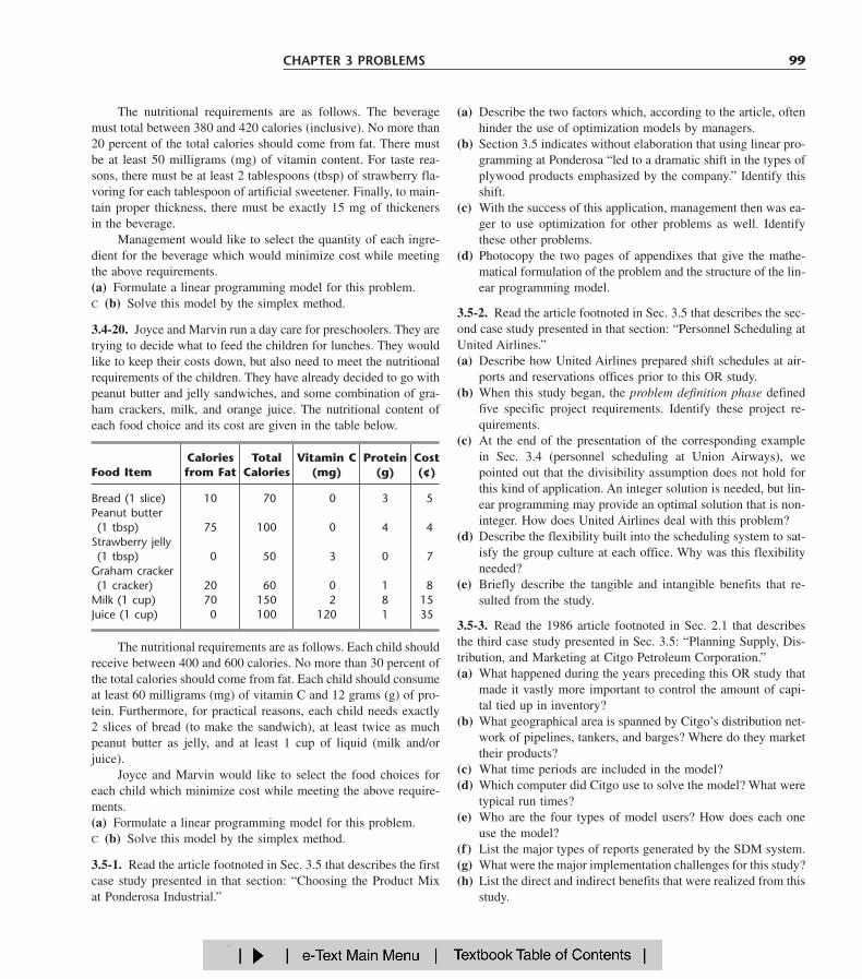
(a) Describe the two factors which, according to the article, oftenhinder the use of optimization models by managers.

(b) Section 3.5 indicates without elaboration that using linear pro-gramming at Ponderosa “led to a dramatic shift in the types ofplywood products emphasized by the company.” Identify thisshift.

(c) With the success of this application, management then was ea-ger to use optimization for other problems as well. Identifythese other problems.

(d) Photocopy the two pages of appendixes that give the mathe-matical formulation of the problem and the structure of the lin-ear programming model.

3.5-2. Read the article footnoted in Sec. 3.5 that describes the sec-ond case study presented in that section: “Personnel Scheduling atUnited Airlines.”(a) Describe how United Airlines prepared shift schedules at air-

ports and reservations offices prior to this OR study.(b) When this study began, the problem definition phase defined

five specific project requirements. Identify these project re-quirements.

(c) At the end of the presentation of the corresponding examplein Sec. 3.4 (personnel scheduling at Union Airways), wepointed out that the divisibility assumption does not hold forthis kind of application. An integer solution is needed, but lin-ear programming may provide an optimal solution that is non-integer. How does United Airlines deal with this problem?

(d) Describe the flexibility built into the scheduling system to sat-isfy the group culture at each office. Why was this flexibilityneeded?

(e) Briefly describe the tangible and intangible benefits that re-sulted from the study.

3.5-3. Read the 1986 article footnoted in Sec. 2.1 that describesthe third case study presented in Sec. 3.5: “Planning Supply, Dis-tribution, and Marketing at Citgo Petroleum Corporation.”(a) What happened during the years preceding this OR study that

made it vastly more important to control the amount of capi-tal tied up in inventory?

(b) What geographical area is spanned by Citgo’s distribution net-work of pipelines, tankers, and barges? Where do they markettheir products?

(c) What time periods are included in the model?(d) Which computer did Citgo use to solve the model? What were

typical run times?(e) Who are the four types of model users? How does each one

use the model?(f) List the major types of reports generated by the SDM system.(g) What were the major implementation challenges for this study?(h) List the direct and indirect benefits that were realized from this

study.

The nutritional requirements are as follows. The beveragemust total between 380 and 420 calories (inclusive). No more than20 percent of the total calories should come from fat. There mustbe at least 50 milligrams (mg) of vitamin content. For taste rea-sons, there must be at least 2 tablespoons (tbsp) of strawberry fla-voring for each tablespoon of artificial sweetener. Finally, to main-tain proper thickness, there must be exactly 15 mg of thickenersin the beverage.

Management would like to select the quantity of each ingre-dient for the beverage which would minimize cost while meetingthe above requirements.(a) Formulate a linear programming model for this problem.C (b) Solve this model by the simplex method.

3.4-20. Joyce and Marvin run a day care for preschoolers. They aretrying to decide what to feed the children for lunches. They wouldlike to keep their costs down, but also need to meet the nutritionalrequirements of the children. They have already decided to go withpeanut butter and jelly sandwiches, and some combination of gra-ham crackers, milk, and orange juice. The nutritional content ofeach food choice and its cost are given in the table below.


The nutritional requirements are as follows. Each child shouldreceive between 400 and 600 calories. No more than 30 percent ofthe total calories should come from fat. Each child should consumeat least 60 milligrams (mg) of vitamin C and 12 grams (g) of pro-tein. Furthermore, for practical reasons, each child needs exactly2 slices of bread (to make the sandwich), at least twice as muchpeanut butter as jelly, and at least 1 cup of liquid (milk and/orjuice).

Joyce and Marvin would like to select the food choices foreach child which minimize cost while meeting the above require-ments.(a) Formulate a linear programming model for this problem.C (b) Solve this model by the simplex method.

3.5-1. Read the article footnoted in Sec. 3.5 that describes the firstcase study presented in that section: “Choosing the Product Mixat Ponderosa Industrial.”

Calories Total Vitamin C Protein CostFood Item from Fat Calories (mg) (g) (¢)

Bread (1 slice) 10 70 0 3 5Peanut butter (1 tbsp) 75 100 0 4 4

Strawberry jelly (1 tbsp) 0 50 3 0 7

Graham cracker (1 cracker) 20 60 0 1 8

Milk (1 cup) 70 150 2 8 15Juice (1 cup) 0 100 120 1 35

(c) Make three guesses of your own choosing for the optimal so-lution. Use the spreadsheet to check each one for feasibilityand, if feasible, to find the value of the objective function.Which feasible guess has the best objective function value?

(d) Use the Excel Solver to solve the model by the simplex method.

3.6-3. You are given the following data for a linear programmingproblem where the objective is to minimize the cost of conductingtwo nonnegative activities so as to achieve three benefits that donot fall below their minimum levels.

3.6-1.* You are given the following data for a linear programmingproblem where the objective is to maximize the profit from allo-cating three resources to two nonnegative activities.


(a) Formulate a linear programming model for this problem.D (b) Use the graphical method to solve this model.(c) Display the model on an Excel spreadsheet.(d) Use the spreadsheet to check the following solutions:

(x1, x2) � (2, 2), (3, 3), (2, 4), (4, 2), (3, 4), (4, 3). Which ofthese solutions are feasible? Which of these feasible solutionshas the best value of the objective function?

C (e) Use the Excel Solver to solve the model by the simplexmethod.

3.6-2. Ed Butler is the production manager for the Bilco Corpo-ration, which produces three types of spare parts for automobiles.The manufacture of each part requires processing on each of twomachines, with the following processing times (in hours):

Each machine is available 40 hours per month. Each part manu-factured will yield a unit profit as follows:

Part

Machine A B C

1 0.02 0.03 0.052 0.05 0.02 0.04

Part

A B C

Profit $50 $40 $30

Benefit Contribution perUnit of Each Activity Minimum

AcceptableBenefit Activity 1 Activity 2 Level

1 5 3 602 2 2 303 7 9 126

Unit cost $60 $50

Kilogram Kilogram Kilogram MinimumNutritional of of of DailyIngredient Corn Tankage Alfalfa Requirement

Carbohydrates 90 20 40 200Protein 30 80 60 180Vitamins 10 20 60 150

Cost (¢) 84 72 60

(a) Formulate a linear programming model for this problem.D (b) Use the graphical method to solve this model.(c) Display the model on an Excel spreadsheet.(d) Use the spreadsheet to check the following solutions:

(x1, x2) � (7, 7), (7, 8), (8, 7), (8, 8), (8, 9), (9, 8). Which ofthese solutions are feasible? Which of these feasible solutionshas the best value of the objective function?

C (e) Use the Excel Solver to solve this model by the simplexmethod.

3.6-4.* Fred Jonasson manages a family-owned farm. To supple-ment several food products grown on the farm, Fred also raisespigs for market. He now wishes to determine the quantities of theavailable types of feed (corn, tankage, and alfalfa) that should begiven to each pig. Since pigs will eat any mix of these feed types,the objective is to determine which mix will meet certain nutri-tional requirements at a minimum cost. The number of units of eachtype of basic nutritional ingredient contained within a kilogram ofeach feed type is given in the following table, along with the dailynutritional requirements and feed costs:

Resource Usage perUnit of Each Activity

Amount of ResourceResource Activity 1 Activity 2 Available

1 2 1 102 3 3 203 2 4 20

Contribution $20 $30per unit

Contribution per unit � profit per unit of the activity.

Ed wants to determine the mix of spare parts to produce in orderto maximize total profit.(a) Formulate a linear programming model for this problem.(b) Display the model on an Excel spreadsheet.

(d) Take a few minutes to use a trial-and-error approach with thespreadsheet to develop your best guess for the optimal solu-tion. What is the total amount invested for your solution?


3.7-1. The Philbrick Company has two plants on opposite sides ofthe United States. Each of these plants produces the same two prod-ucts and then sells them to wholesalers within its half of the coun-try. The orders from wholesalers have already been received forthe next 2 months (February and March), where the number ofunits requested are shown below. (The company is not obligatedto completely fill these orders but will do so if it can without de-creasing its profits.)

(a) Formulate a linear programming model for this problem.(b) Display the model on an Excel spreadsheet.(c) Use the spreadsheet to check if (x1, x2, x3) � (1, 2, 2) is a fea-

sible solution and, if so, what the daily cost would be for thisdiet. How many units of each nutritional ingredient would thisdiet provide daily?

(d) Take a few minutes to use a trial-and-error approach with thespreadsheet to develop your best guess for the optimal solu-tion. What is the daily cost for your solution?


3.6-5. Maureen Laird is the chief financial officer for the AlvaElectric Co., a major public utility in the midwest. The companyhas scheduled the construction of new hydroelectric plants 5, 10,and 20 years from now to meet the needs of the growing popu-lation in the region served by the company. To cover at least theconstruction costs, Maureen needs to invest some of the com-pany’s money now to meet these future cash-flow needs. Mau-reen may purchase only three kinds of financial assets, each ofwhich costs $1 million per unit. Fractional units may be pur-chased. The assets produce income 5, 10, and 20 years from now,and that income is needed to cover at least minimum cash-flowrequirements in those years. (Any excess income above the min-imum requirement for each time period will be used to increasedividend payments to shareholders rather than saving it to helpmeet the minimum cash-flow requirement in the next time pe-riod.) The following table shows both the amount of income gen-erated by each unit of each asset and the minimum amount of in-come needed for each of the future time periods when a newhydroelectric plant will be constructed.


Maureen wishes to determine the mix of investments in these as-sets that will cover the cash-flow requirements while minimizingthe total amount invested.(a) Formulate a linear programming model for this problem.(b) Display the model on a spreadsheet.(c) Use the spreadsheet to check the possibility of purchasing 100

units of Asset 1, 100 units of Asset 2, and 200 units of Asset3. How much cash flow would this mix of investments gener-ate 5, 10, and 20 years from now? What would be the totalamount invested?

Income per Unit of AssetMinimum Cash

Year Asset 1 Asset 2 Asset 3 Flow Required

5 $2 million $1 million $0.5 million $400 million10 $0.5 million $0.5 million $1 million $100 million20 0 $1.5 million $2 million $300 million

Each plant has 20 production days available in February and 23production days available in March to produce and ship these prod-ucts. Inventories are depleted at the end of January, but each planthas enough inventory capacity to hold 1,000 units total of the twoproducts if an excess amount is produced in February for sale inMarch. In either plant, the cost of holding inventory in this way is$3 per unit of product 1 and $4 per unit of product 2.

Each plant has the same two production processes, each ofwhich can be used to produce either of the two products. The pro-duction cost per unit produced of each product is shown below foreach process in each plant.

The production rate for each product (number of units producedper day devoted to that product) also is given below for each processin each plant.

Plant 1 Plant 2

Product February March February March

1 3,600 6,300 4,900 4,2002 4,500 5,400 5,100 6,000

Plant 1 Plant 2

Product Process 1 Process 2 Process 1 Process 2

1 $62 $59 $61 $652 $78 $85 $89 $86

Plant 1 Plant 2

Product Process 1 Process 2 Process 1 Process 2

1 100 140 130 1102 120 150 160 130

C 3.7-6. Reconsider Prob. 3.6-4.(a) Use MPL/CPLEX to formulate and solve the model for this

problem.(b) Use LINGO to formulate and solve this model.



3.7-8. A large paper manufacturing company, the Quality PaperCorporation, has 10 paper mills from which it needs to supply 1,000customers. It uses three alternative types of machines and four typesof raw materials to make five different types of paper. Therefore,the company needs to develop a detailed production distributionplan on a monthly basis, with an objective of minimizing the totalcost of producing and distributing the paper during the month.Specifically, it is necessary to determine jointly the amount of eachtype of paper to be made at each paper mill on each type of ma-chine and the amount of each type of paper to be shipped fromeach paper mill to each customer.

The relevant data can be expressed symbolically as follows:

Djk � number of units of paper type k demanded by custo-mer j,

rklm � number of units of raw material m needed to produce1 unit of paper type k on machine type l,

Rim � number of units of raw material m available at papermill i,

ckl � number of capacity units of machine type l that willproduce 1 unit of paper type k,

Cil � number of capacity units of machine type l availableat paper mill i,

Pikl � production cost for each unit of paper type k producedon machine type l at paper mill i,

Tijk � transportation cost for each unit of paper type k shippedfrom paper mill i to customer j.

(a) Using these symbols, formulate a linear programming modelfor this problem by hand.

(b) How many functional constraints and decision variables doesthis model have?

C (c) Use MPL to formulate this problem.C (d) Use LINGO to formulate this problem.

The net sales revenue (selling price minus normal shippingcosts) the company receives when a plant sells the products to itsown customers (the wholesalers in its half of the country) is $83per unit of product 1 and $112 per unit of product 2. However, italso is possible (and occasionally desirable) for a plant to make ashipment to the other half of the country to help fill the sales ofthe other plant. When this happens, an extra shipping cost of $9per unit of product 1 and $7 per unit of product 2 is incurred.

Management now needs to determine how much of each prod-uct should be produced by each production process in each plantduring each month, as well as how much each plant should sell ofeach product in each month and how much each plant should shipof each product in each month to the other plant’s customers. Theobjective is to determine which feasible plan would maximize thetotal profit (total net sales revenue minus the sum of the produc-tion costs, inventory costs, and extra shipping costs).(a) Formulate a complete linear programming model in algebraic

form that shows the individual constraints and decision vari-ables for this problem.

C (b) Formulate this same model on an Excel spreadsheet instead.Then use the Excel Solver to solve the model.

C (c) Use MPL to formulate this model in a compact form. Thenuse the MPL solver CPLEX to solve the model.

C (d) Use LINGO to formulate this model in a compact form.Then use the LINGO solver to solve the model.










Automobile Alliance, a large automobile manufacturing company, organizes the vehi-cles it manufactures into three families: a family of trucks, a family of small cars, anda family of midsized and luxury cars. One plant outside Detroit, MI, assembles twomodels from the family of midsized and luxury cars. The first model, the FamilyThrillseeker, is a four-door sedan with vinyl seats, plastic interior, standard features,and excellent gas mileage. It is marketed as a smart buy for middle-class families withtight budgets, and each Family Thrillseeker sold generates a modest profit of $3,600for the company. The second model, the Classy Cruiser, is a two-door luxury sedanwith leather seats, wooden interior, custom features, and navigational capabilities. It ismarketed as a privilege of affluence for upper-middle-class families, and each ClassyCruiser sold generates a healthy profit of $5,400 for the company.

Rachel Rosencrantz, the manager of the assembly plant, is currently deciding theproduction schedule for the next month. Specifically, she must decide how many Fam-ily Thrillseekers and how many Classy Cruisers to assemble in the plant to maximizeprofit for the company. She knows that the plant possesses a capacity of 48,000 labor-hours during the month. She also knows that it takes 6 labor-hours to assemble oneFamily Thrillseeker and 10.5 labor-hours to assemble one Classy Cruiser.

Because the plant is simply an assembly plant, the parts required to assemble thetwo models are not produced at the plant. They are instead shipped from other plantsaround the Michigan area to the assembly plant. For example, tires, steering wheels,windows, seats, and doors all arrive from various supplier plants. For the next month,Rachel knows that she will be able to obtain only 20,000 doors (10,000 left-hand doorsand 10,000 right-hand doors) from the door supplier. A recent labor strike forced theshutdown of that particular supplier plant for several days, and that plant will not beable to meet its production schedule for the next month. Both the Family Thrillseekerand the Classy Cruiser use the same door part.

In addition, a recent company forecast of the monthly demands for different au-tomobile models suggests that the demand for the Classy Cruiser is limited to 3,500cars. There is no limit on the demand for the Family Thrillseeker within the capacitylimits of the assembly plant.

(a) Formulate and solve a linear programming problem to determine the number of FamilyThrillseekers and the number of Classy Cruisers that should be assembled.

Before she makes her final production decisions, Rachel plans to explore the follow-ing questions independently except where otherwise indicated.

(b) The marketing department knows that it can pursue a targeted $500,000 advertising cam-paign that will raise the demand for the Classy Cruiser next month by 20 percent. Shouldthe campaign be undertaken?

(c) Rachel knows that she can increase next month’s plant capacity by using overtime labor. Shecan increase the plant’s labor-hour capacity by 25 percent. With the new assembly plant ca-pacity, how many Family Thrillseekers and how many Classy Cruisers should be assembled?

(d) Rachel knows that overtime labor does not come without an extra cost. What is the maxi-mum amount she should be willing to pay for all overtime labor beyond the cost of this la-bor at regular time rates? Express your answer as a lump sum.

CASE 3.1 AUTO ASSEMBLY 103

CASE 3.1 AUTO ASSEMBLY

(e) Rachel explores the option of using both the targeted advertising campaign and the overtimelabor-hours. The advertising campaign raises the demand for the Classy Cruiser by 20 per-cent, and the overtime labor increases the plant’s labor-hour capacity by 25 percent. Howmany Family Thrillseekers and how many Classy Cruisers should be assembled using theadvertising campaign and overtime labor-hours if the profit from each Classy Cruiser soldcontinues to be 50 percent more than for each Family Thrillseeker sold?

(f) Knowing that the advertising campaign costs $500,000 and the maximum usage of overtimelabor-hours costs $1,600,000 beyond regular time rates, is the solution found in part (e) awise decision compared to the solution found in part (a)?

(g) Automobile Alliance has determined that dealerships are actually heavily discounting theprice of the Family Thrillseekers to move them off the lot. Because of a profit-sharing agree-ment with its dealers, the company is therefore not making a profit of $3,600 on the Fam-ily Thrillseeker but is instead making a profit of $2,800. Determine the number of FamilyThrillseekers and the number of Classy Cruisers that should be assembled given this newdiscounted price.

(h) The company has discovered quality problems with the Family Thrillseeker by randomlytesting Thrillseekers at the end of the assembly line. Inspectors have discovered that in over60 percent of the cases, two of the four doors on a Thrillseeker do not seal properly. Be-cause the percentage of defective Thrillseekers determined by the random testing is so high,the floor supervisor has decided to perform quality control tests on every Thrillseeker at theend of the line. Because of the added tests, the time it takes to assemble one FamilyThrillseeker has increased from 6 to 7.5 hours. Determine the number of units of each modelthat should be assembled given the new assembly time for the Family Thrillseeker.

(i) The board of directors of Automobile Alliance wishes to capture a larger share of the luxurysedan market and therefore would like to meet the full demand for Classy Cruisers. They askRachel to determine by how much the profit of her assembly plant would decrease as com-pared to the profit found in part (a). They then ask her to meet the full demand for ClassyCruisers if the decrease in profit is not more than $2,000,000.

( j) Rachel now makes her final decision by combining all the new considerations described inparts ( f ), (g), and (h). What are her final decisions on whether to undertake the advertisingcampaign, whether to use overtime labor, the number of Family Thrillseekers to assemble,and the number of Classy Cruisers to assemble?


A cafeteria at All-State University has one special dish it serves like clockwork everyThursday at noon. This supposedly tasty dish is a casserole that contains sautéed onions,boiled sliced potatoes, green beans, and cream of mushroom soup. Unfortunately, stu-dents fail to see the special quality of this dish, and they loathingly refer to it as the KillerCasserole. The students reluctantly eat the casserole, however, because the cafeteria pro-vides only a limited selection of dishes for Thursday’s lunch (namely, the casserole).

Maria Gonzalez, the cafeteria manager, is looking to cut costs for the coming year,and she believes that one sure way to cut costs is to buy less expensive and perhapslower-quality ingredients. Because the casserole is a weekly staple of the cafeteriamenu, she concludes that if she can cut costs on the ingredients purchased for the casse-role, she can significantly reduce overall cafeteria operating costs. She therefore de-

CASE 3.2 CUTTING CAFETERIA COSTS

cides to invest time in determining how to minimize the costs of the casserole whilemaintaining nutritional and taste requirements.

Maria focuses on reducing the costs of the two main ingredients in the casserole,the potatoes and green beans. These two ingredients are responsible for the greatestcosts, nutritional content, and taste of the dish.

Maria buys the potatoes and green beans from a wholesaler each week. Potatoescost $0.40 per pound, and green beans cost $1.00 per pound.

All-State University has established nutritional requirements that each main dishof the cafeteria must meet. Specifically, the total amount of the dish prepared for allthe students for one meal must contain 180 grams (g) of protein, 80 milligrams (mg)of iron, and 1,050 mg of vitamin C. (There are 453.6 g in 1 lb and 1,000 mg in 1 g.)For simplicity when planning, Maria assumes that only the potatoes and green beanscontribute to the nutritional content of the casserole.

Because Maria works at a cutting-edge technological university, she has been ex-posed to the numerous resources on the World Wide Web. She decides to surf the Webto find the nutritional content of potatoes and green beans. Her research yields the fol-lowing nutritional information about the two ingredients:

CASE 3.2 CUTTING CAFETERIA COSTS 105

Edson Branner, the cafeteria cook who is surprisingly concerned about taste, in-forms Maria that an edible casserole must contain at least a six to five ratio in theweight of potatoes to green beans.

Given the number of students who eat in the cafeteria, Maria knows that she mustpurchase enough potatoes and green beans to prepare a minimum of 10 kilograms (kg)of casserole each week. (There are 1,000 g in 1 kg.) Again for simplicity in planning,she assumes that only the potatoes and green beans determine the amount of casserolethat can be prepared. Maria does not establish an upper limit on the amount of casse-role to prepare, since she knows all leftovers can be served for many days thereafteror can be used creatively in preparing other dishes.

(a) Determine the amount of potatoes and green beans Maria should purchase each week forthe casserole to minimize the ingredient costs while meeting nutritional, taste, and demandrequirements.

Before she makes her final decision, Maria plans to explore the following questionsindependently except where otherwise indicated.

(b) Maria is not very concerned about the taste of the casserole; she is only concerned aboutmeeting nutritional requirements and cutting costs. She therefore forces Edson to change therecipe to allow for only at least a one to two ratio in the weight of potatoes to green beans.Given the new recipe, determine the amount of potatoes and green beans Maria should pur-chase each week.

Potatoes Green Beans

Protein 1.5 g per 100 g 5.67 g per 10 ouncesIron 0.3 mg per 100 g 3.402 mg per 10 ouncesVitamin C 12 mg per 100 g 28.35 mg per 10 ounces

(There are 28.35 g in 1 ounce.)

(c) Maria decides to lower the iron requirement to 65 mg since she determines that the other in-gredients, such as the onions and cream of mushroom soup, also provide iron. Determinethe amount of potatoes and green beans Maria should purchase each week given this newiron requirement.

(d) Maria learns that the wholesaler has a surplus of green beans and is therefore selling thegreen beans for a lower price of $0.50 per lb. Using the same iron requirement from part(c) and the new price of green beans, determine the amount of potatoes and green beansMaria should purchase each week.

(e) Maria decides that she wants to purchase lima beans instead of green beans since lima beansare less expensive and provide a greater amount of protein and iron than green beans. Mariaagain wields her absolute power and forces Edson to change the recipe to include lima beansinstead of green beans. Maria knows she can purchase lima beans for $0.60 per lb from thewholesaler. She also knows that lima beans contain 22.68 g of protein per 10 ounces of limabeans, 6.804 mg of iron per 10 ounces of lima beans, and no vitamin C. Using the new costand nutritional content of lima beans, determine the amount of potatoes and lima beans Mariashould purchase each week to minimize the ingredient costs while meeting nutritional, taste,and demand requirements. The nutritional requirements include the reduced iron requirementfrom part (c).

(f ) Will Edson be happy with the solution in part (e)? Why or why not?(g) An All-State student task force meets during Body Awareness Week and determines that All-

State University’s nutritional requirements for iron are too lax and that those for vitamin Care too stringent. The task force urges the university to adopt a policy that requires eachserving of an entrée to contain at least 120 mg of iron and at least 500 mg of vitamin C.Using potatoes and lima beans as the ingredients for the dish and using the new nutritionalrequirements, determine the amount of potatoes and lima beans Maria should purchase eachweek.


California Children’s Hospital has been receiving numerous customer complaints be-cause of its confusing, decentralized appointment and registration process. When cus-tomers want to make appointments or register child patients, they must contact theclinic or department they plan to visit. Several problems exist with this current strat-egy. Parents do not always know the most appropriate clinic or department they mustvisit to address their children’s ailments. They therefore spend a significant amount oftime on the phone being transferred from clinic to clinic until they reach the most ap-propriate clinic for their needs. The hospital also does not publish the phone numbersof all clinic and departments, and parents must therefore invest a large amount of timein detective work to track down the correct phone number. Finally, the various clinicsand departments do not communicate with each other. For example, when a doctorschedules a referral with a colleague located in another department or clinic, that de-partment or clinic almost never receives word of the referral. The parent must contactthe correct department or clinic and provide the needed referral information.

CASE 3.3 STAFFING A CALL CENTER1

1This case is based on an actual project completed by a team of master’s students in the Department of En-gineering-Economic Systems and Operations Research at Stanford University.

In efforts to reengineer and improve its appointment and registration process, thechildren’s hospital has decided to centralize the process by establishing one call cen-ter devoted exclusively to appointments and registration. The hospital is currently inthe middle of the planning stages for the call center. Lenny Davis, the hospital man-ager, plans to operate the call center from 7 A.M. to 9 P.M. during the weekdays.

Several months ago, the hospital hired an ambitious management consulting firm,Creative Chaos Consultants, to forecast the number of calls the call center would re-ceive each hour of the day. Since all appointment and registration-related calls wouldbe received by the call center, the consultants decided that they could forecast the callsat the call center by totaling the number of appointment and registration-related callsreceived by all clinics and departments. The team members visited all the clinics anddepartments, where they diligently recorded every call relating to appointments andregistration. They then totaled these calls and altered the totals to account for callsmissed during data collection. They also altered totals to account for repeat calls thatoccurred when the same parent called the hospital many times because of the confu-sion surrounding the decentralized process. Creative Chaos Consultants determined theaverage number of calls the call center should expect during each hour of a weekday.The following table provides the forecasts.

CASE 3.3 STAFFING A CALL CENTER 107

After the consultants submitted these forecasts, Lenny became interested in the per-centage of calls from Spanish speakers since the hospital services many Spanish pa-tients. Lenny knows that he has to hire some operators who speak Spanish to handlethese calls. The consultants performed further data collection and determined that onaverage, 20 percent of the calls were from Spanish speakers.

Given these call forecasts, Lenny must now decide how to staff the call center dur-ing each 2 hour shift of a weekday. During the forecasting project, Creative Chaos Con-sultants closely observed the operators working at the individual clinics and depart-ments and determined the number of calls operators process per hour. The consultantsinformed Lenny that an operator is able to process an average of six calls per hour.Lenny also knows that he has both full-time and part-time workers available to staffthe call center. A full-time employee works 8 hours per day, but because of paperworkthat must also be completed, the employee spends only 4 hours per day on the phone.To balance the schedule, the employee alternates the 2-hour shifts between answeringphones and completing paperwork. Full-time employees can start their day either byanswering phones or by completing paperwork on the first shift. The full-time em-

Work Shift Average Number of Calls

7 A.M.–9 A.M. 40 calls per hour9 A.M.–11 A.M. 85 calls per hour

11 A.M.–1 P.M. 70 calls per hour1 P.M.–3 P.M. 95 calls per hour3 P.M.–5 P.M. 80 calls per hour5 P.M.–7 P.M. 35 calls per hour7 P.M.–9 P.M. 10 calls per hour

ployees speak either Spanish or English, but none of them are bilingual. Both Span-ish-speaking and English-speaking employees are paid $10 per hour for work before5 P.M. and $12 per hour for work after 5 P.M. The full-time employees can begin workat the beginning of the 7 A.M. to 9 A.M. shift, 9 A.M. to 11 A.M. shift, 11 A.M. to 1 P.M.shift, or 1 P.M. to 3 P.M. shift. The part-time employees work for 4 hours, only answercalls, and only speak English. They can start work at the beginning of the 3 P.M. to5 P.M. shift or the 5 P.M. to 7 P.M. shift, and like the full-time employees, they are paid$10 per hour for work before 5 P.M. and $12 per hour for work after 5 P.M.

For the following analysis consider only the labor cost for the time employeesspend answering phones. The cost for paperwork time is charged to other cost centers.

(a) How many Spanish-speaking operators and how many English-speaking operators does thehospital need to staff the call center during each 2-hour shift of the day in order to answerall calls? Please provide an integer number since half a human operator makes no sense.

(b) Lenny needs to determine how many full-time employees who speak Spanish, full-time em-ployees who speak English, and part-time employees he should hire to begin on each shift.Creative Chaos Consultants advise him that linear programming can be used to do this insuch a way as to minimize operating costs while answering all calls. Formulate a linear pro-gramming model of this problem.

(c) Obtain an optimal solution for the linear programming model formulated in part (b) to guideLenny’s decision.

(d) Because many full-time workers do not want to work late into the evening, Lenny can findonly one qualified English-speaking operator willing to begin work at 1 P.M. Given this newconstraint, how many full-time English-speaking operators, full-time Spanish-speaking op-erators, and part-time operators should Lenny hire for each shift to minimize operating costswhile answering all calls?

(e) Lenny now has decided to investigate the option of hiring bilingual operators instead ofmonolingual operators. If all the operators are bilingual, how many operators should be work-ing during each 2-hour shift to answer all phone calls? As in part (a), please provide an in-teger answer.

(f) If all employees are bilingual, how many full-time and part-time employees should Lennyhire to begin on each shift to minimize operating costs while answering all calls? As in part(b), formulate a linear programming model to guide Lenny’s decision.

(g) What is the maximum percentage increase in the hourly wage rate that Lenny can pay bilin-gual employees over monolingual employees without increasing the total operating costs?

(h) What other features of the call center should Lenny explore to improve service or minimizeoperating costs?


3 Introduction to Linear Programming - OHIO Personal Websites

Documents

Transcript of 3 Introduction to Linear Programming - OHIO Personal Websites