OHIO HARDWOOD SAWLOG PRICE TRENDS

OHIO HARDWOOD SAWLOG PRICE TRENDS

Raymond P. DuvalGraduate Student

E-mail: [email protected]

T. Eric McConnell*{Assistant Professor and Extension Specialist


David M. HixAssociate Professor


Stephen N. MatthewsAssistant Professor


Roger A. WilliamsAssociate Professor

School of Environment and Natural Resources

The Ohio State University

Columbus, OH 43210


(Received July 2013)

Abstract. We examined the 52-yr sawlog price trends for the 10 commercial hardwood tree species in

Ohio. Data were compiled from the Ohio Timber Price Report for four log grades (Prime, #1, #2,

Blocking) covering the years 1960–2011, and average annual percentage rates of change in both nominal

and real sawlog prices were determined. We further compared real log grade price movements within each

species. Nominal prices for all log grades of all species increased at significant annual rates. However,

real price change rates varied with approximately two-thirds of the species–grade combinations not

significantly differing from zero. Real Blocking log prices declined at significant annual rates for seven

species. Only white oak contained log grades (Prime and #1 only) with significantly increasing real prices.

Four groups were identified based on differences observed, or not observed, when comparing initial price

levels of log grades and rates of change within each species. Initial price differences generally occurred

between the higher (Prime and #1) and lower (#2 and Blocking) grade logs. Rate of price change

differences were more a result of declining Blocking log prices than increasing high-grade log prices with

the exception of white oak.

Keywords: Appalachian roundwood markets, hardwood log prices, Ohio forest industry, timber markets.

INTRODUCTION

Industrial product demand and new home con-struction are main drivers of forest products pro-duction and profits in the US (Barrett 2013).

These influences have greatly affected wood useand manufacturing in recent times. The housingcrash and recent great recession compounded analready decreasing economic performance. Themore gradual decline can be partially attributedto furniture and pulp and paper manufacturersmoving portions of their operations overseas dur-ing the past two decades and a subsequent overall

* Corresponding author{ SWST member

Wood and Fiber Science, 46(1), 2014, pp. 85-96# 2014 by the Society of Wood Science and Technology

rise in market share of imported forest-basedproducts (Espinoza et al 2011).

The forest products industry has been experienc-ing significant change, however, for quite sometime. In the past, softwood-based producers gen-erally owned mills and land that were used formaintaining a supply of stumpage. This verticalbusiness arrangement has changed with time toa market-based model in which mills competefor stumpage directly (Hickman 2007). Like-wise, the hardwood sector has seen technologyset the pace for changes businesses have experi-enced from the 1970s to today, along with ashifting combination of end uses for hardwoodproducts (Luppold and Baumgras 1996). Someof these technological advances have increasedmills’ abilities to extract profitable lumber fromlower quality logs. Prices for zero clear facelogs, for example, have recently become morecompetitive with higher quality logs because ofadvances in lumber recovery capabilities (Brianand Chapman 2005).

Price expectations play a direct role in mill pur-chasing decisions (Guttenberg 1970). Havingthe ability to estimate historic price changes ata projected rate, as well as forecasting long-termand short-term trends in species popularity, canaffect which species and/or log grades buyersmay pursue. Purchasing decisions made withoutan understanding of possible future price changescan lead to production runs that fail to maximizeprofits or minimize losses. Log-linear regressionhas been used to describe the evolving trends instumpage, sawlog, and lumber prices in multiplestates and regions (Luppold and Baumgras 1995,2007; Linehan et al 2003; Wagner and Sendak2005). Price trends examined with time can pro-vide information for future business decisionsonce a rate of price change is determined.

Ohio log prices in the past have provided a basisfor investigating hardwood market trends(Luppold and Baumgras 1996; Luppold et al1998). However, these studies encompassedprice reporting periods of not more than 20 yrand investigated only particular species andmarkets. To date, no comprehensive study of

sawlog prices has been performed for Ohio.Although recent research conducted in neighbor-ing states and regions (Campbell and White1989; Irland et al 2001; Linehan et al 2003;Linehan and Jacobson 2005; Hoover and Preston2013) is useful for developing price trends on abroader scale, describing Ohio market activitiesrequires analysis at a more local level. The OhioTimber Price Report (Ohio DNR 2013; OSUE2013), which has continually tracked gradedlog prices since 1960, provides a basis for deter-mining average annual percentage rates ofchange (APR) in hardwood sawlog prices. The52-yr APR are currently unknown and requirefurther investigation.

The goal of this research was to describe the pricetrends from 1960-2011 for hardwood sawlogs ofthe commercial timber species reported in theOhio Timber Price Report. Autoregressive func-tions were used to determine APR for the four loggrades—Prime, #1, #2, and Blocking—reportedwithin the 10 species. Price movements betweengrades for each species were then comparedto determine if differences existed.

METHODOLOGY

Data

The data used here were compiled from bian-nual surveys sent to loggers, mills, and timberbuyers in Ohio in May and November. Sawlogprices are reported for 10 species: ash (Fraxinusspp.), basswood (Tilia americana), black cherry(Prunus serotina), hard and soft maples (Acerspp.), hickory (Carya spp.), black walnut(Juglans nigra), red and white oaks (Quercusspp.), and yellow-poplar (Liriodendron tulipifera).Prices for four log grades were tracked withineach species: Prime, #1, #2, and Blocking withPrime being the highest grade and Blocking thelowest. Average prices paid (dollars per thousandboard feet, Doyle) are provided in each report.

From 1960 to 2001, surveys were conducted bythe Ohio Agricultural Statistics Service and DNR(Ohio DNR 2013). From 2003 to the present,Ohio State University Extension has overseen

86 WOOD AND FIBER SCIENCE, JANUARY 2014, V. 46(1)

the program (OSUE 2013). During the transitionyear of 2002, no surveys were distributed. Wetreated these missing 2002 data as missingcompletely at random (MCAR). MCAR is theprobability a missing observation Xi is unrelatedto its value or to the value of any other variablespresent. The treatment applied for the missingdata are simple listwise deletion, which is omis-sion of the absent cases and analyzing whatremains (Howell 2012).

Analyses

We used a simple linear regression model fol-lowing a natural logarithm transformation of eachspecies’ log grade price data to evaluate pricetrends from 1960 to 2011. The rate of pricechange was found using Eq 1:

Y ¼ b0 þ b1xt þ e ½1�

where Y ¼ ln(Pt) with Pt being the average priceof a log grade paid at time t; the intercept of theline, b0, represented the initial price in a series;b1 represented the slope, or the continuous rateof change in price; xt was a price report at time tin a series; and e represented the model’s error.The continuous rate, b1, was then converted toan annualized rate i using Eq 2 (Wagner andSendak 2005):

i ¼ eb1 � 1� � � 100 ½2�

One concern when analyzing time-series datawas autocorrelation, which describes the ten-dency of the data’s residuals to be similar toadjacent points (Moineddin et al 2003). Thisdisrupts the assumption in linear regression thatthe residuals of each observation are indepen-dent (Linehan and Jacobson 2005). The poten-tial presence of autocorrelation was examinedby applying the Durbin–Watson test statistic,which tests the assumption of independence ofa linear regression’s residuals (Albright et al1999). We found that significant autocorre-lation existed across each series of data withall testing conducted using SAS software Ver-

sion 9.2 (SAS 2008) at a significance level ofa ¼ 0.05.

We used maximum likelihood stepwise auto-regression to account for the autocorrelation(Luppold et al 1998; Linehan et al 2003; Wagnerand Sendak 2005; Zhou and Buongiorno 2006;Luppold and Bumgardner 2007; Malaty et al2007; Mei et al 2010). Using a backward step-wise approach, a number of lag variables wasassigned in a group and insignificant variableswere removed one at a time. Any remainingvariables were those significantly contributingto the model. Five lag variables were applied toour data, and we found a maximum of three wasneeded for an individual series to account for theautocorrelated data.

We determined the APR for nominal and realprices of each species’ four log grades duringthe entire reporting period. All nominal priceswere adjusted for inflation to a base year of 1982using the producer price index for all commodi-ties (US Department of Labor Bureau of LaborStatistics 2013). To give a sense of sawlog pricechanges relative to the general economy, theAPR of both state and national gross domesticproducts (GDPs), which charted the values offinal goods and services produced in Ohio from1963 to 2011 and in the US from 1960 to 2011,were calculated (US Department of CommerceBureau of Economic Analysis 2013a, 2013b,2013c). Additionally, the APR of a 10-yr Trea-sury bond’s annually aggregated constant matu-rity rate from 1962 to 2011 was determined toprovide a comparison of an alternative invest-ment (Federal Reserve 2013).

Real prices were then compared among gradeswithin each species for initial price and APRdifferences. This was done by adding an indica-tor variable to a regression function to differen-tiate between grades using Eq 3:

Yt ¼ b0 þ b1x1t þ b2x2t þ b3x1tx2t þ e ½3�

where Y ¼ ln(Pt) with Pt being the average priceof a log grade paid at time t; x1t was a pricereport at time t in a series; x2t was the indicator

Duval et al—OHIO HARDWOOD SAWLOG PRICE TRENDS 87

variable (1 for the grade of interest, 0 for thedefault grade); x1tx2t was the interaction term;and b0, b1, b2, and b3 were model coefficientswith e being the model’s error. The indicatorvariable coefficient, b2, tested if the initialprices between two grades were different. Theinteraction coefficient, b3, tested for an APRdifference among grades. Autocorrelation wasagain examined and accounted for as describedpreviously. Autoregression model errors werereported as percentage root mean square error(%RMSE) using Eq 4 (Linehan et al 2003;Linehan and Jacobson 2005):

%RMSE ¼ eRMSE � 1� � � 100 ½4�

RESULTS

52-yr Trends by Log Grade

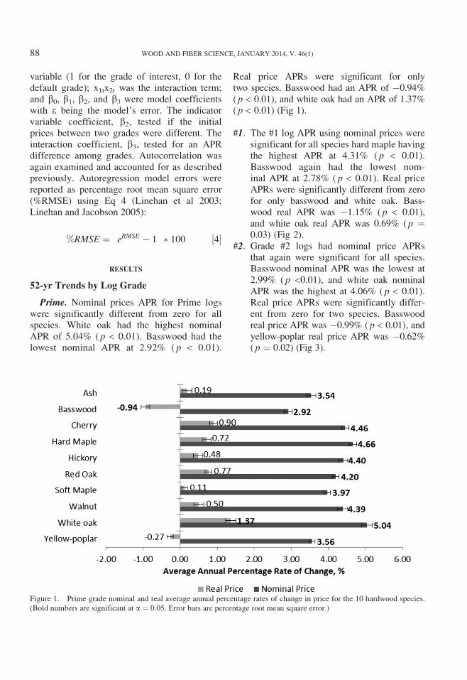
Prime. Nominal prices APR for Prime logswere significantly different from zero for allspecies. White oak had the highest nominalAPR of 5.04% ( p < 0.01). Basswood had thelowest nominal APR at 2.92% ( p < 0.01).

Real price APRs were significant for onlytwo species. Basswood had an APR of �0.94%( p < 0.01), and white oak had an APR of 1.37%( p < 0.01) (Fig 1).

#1. The #1 log APR using nominal prices weresignificant for all species hard maple havingthe highest APR at 4.31% ( p < 0.01).Basswood again had the lowest nom-inal APR at 2.78% ( p < 0.01). Real priceAPRs were significantly different from zerofor only basswood and white oak. Bass-wood real APR was �1.15% ( p < 0.01),and white oak real APR was 0.69% ( p ¼0.03) (Fig 2).

#2. Grade #2 logs had nominal price APRsthat again were significant for all species.Basswood nominal APR was the lowest at2.99% ( p <0.01), and white oak nominalAPR was the highest at 4.06% ( p < 0.01).Real price APRs were significantly differ-ent from zero for two species. Basswoodreal price APR was �0.99% ( p < 0.01), andyellow-poplar real price APR was �0.62%( p ¼ 0.02) (Fig 3).

Figure 1. Prime grade nominal and real average annual percentage rates of change in price for the 10 hardwood species.

(Bold numbers are significant at a ¼ 0.05. Error bars are percentage root mean square error.)


Blocking. Nominal price APR for all speciesof Blocking grade logs were significantly differ-ent from zero. Basswood again had the lowestAPR at 3.17% ( p < 0.01), whereas white oak

had the highest APR at 3.50 ( p < 0.01). Realprice APRs were significant for basswood,cherry, hard maple, hickory, soft maple, walnut,and yellow-poplar. Of these, cherry had the

Figure 2. #1 grade nominal and real average annual percentage rates of change in price for the 10 hardwood species.


Figure 3. #2 grade nominal and real average annual percentage rates of change in price for the 10 hardwood species.

(Bold numbers are significant at a ¼ 0.05. Error bars are percentage root mean square error).


highest real price APR at �0.44% ( p ¼ 0.02),whereas walnut had the lowest real price APRat �0.82% ( p ¼ 0.04) (Fig 4).

Gross Domestic Product and Treasury Trends

Nominal GDP APRwere significant for both Ohio(5.78%, p < 0.01) and the US (6.82%, p < 0.01,Fig 5). Real GDP also significantly increased atAPR of 1.86% for Ohio ( p < 0.01) and 3.06% forthe US ( p < 0.01). Across grades, both nominaland real APR for Ohio’s hardwood sawlogs werelower than those for GDP. The 10-yr Treasurybond’s nominal maturity rate decreased at anAPR of �0.74%, but this was not significantlydifferent from zero. The real maturity rate, how-ever, significantly decreased �4.53% ( p < 0.01,Fig 5). All nominal and real species log gradeAPRs were higher than those of the 10-yrTreasury bonds.

Grade Comparisons within Species

Comparing initial price levels and price trendsamong grades for each hardwood species identi-

fied four separate groups. Group 1 was comprisedof species containing grades in which both initialprices and APR differed. Species in Group 2exhibited varying price levels among grades butno APR differences. Group 3 contained gradeswith differing APR only. In Group 4, neitherAPR nor initial prices significantly differedamong grades (Table 1).

Group 1. Group 1 consisted of cherry, hardmaple, and white oak. Differing initial pricesand APR were found among some grades withineach of these species. In general, these differ-ences occurred between higher grade and lowergrade logs. Both cherry and hard maple hadinitial price and APR differences between Primeand Blocking and between #1 and Blocking.White oak log initial prices and APR showeddifferences between Prime and #2, Prime andBlocking, and #1 and Blocking. Additionally,#2 and Blocking differed by APR only.

Group 2. Group 2 consisted of species withdiffering initial prices among grades but no dif-ferences in APR (ash, basswood, soft maple,walnut, and yellow-poplar). Given the lack of

Figure 4. Blocking grade nominal and real average annual percentage rates of change in price for the 10 hardwood species.



APR differences, these species’ log prices havehistorically not been diverging or convergingamong grades. These significant price spreadshave been maintained across the reportingperiod. Ash had initial price differences betweenPrime and Blocking and between #1 andBlocking. Basswood, soft maple, and yellow-poplar had initial price differences between thehigher grade (Prime and #1) and lower grade(#2 and Blocking) logs but no differencesbetween Prime and #1 or between #2 andBlocking. Walnut initial prices differed in allcombinations containing #2 and Blocking logs.

Group 3. Red oak was found to have no dif-ferences in initial prices among log grades, butAPR differences occurred. These were foundbetween Prime and Blocking logs ( p ¼ 0.03)and between #1 and Blocking logs ( p ¼ 0.04).Red oak did not possess a log grade with an APRsignificantly different from zero (Figs 1–4).However, APR differences found in this studymay be attributed to Blocking log prices chang-ing at a level of significance greater than the

other log grades (Blocking p ¼ 0.07; Prime p ¼0.32; #1 p ¼ 0.35; #2 p ¼ 0.61).

Group 4. Hickory was the only species withno significant differences found among gradesin either initial prices or APR. Possibly, a com-bination of poorer tree quality and lack of mar-kets locally were responsible for these absences.

DISCUSSION

Since 1960, nominal prices have been signifi-cantly increasing for all grades of all species.Real prices, however, have significantly changedfor only one-third of the individual species–gradecombinations and were at times negative. Ofthose, basswood was the only species with APRsignificantly different from zero across loggrades, all of which were negative. Cherry, hardmaple, hickory, soft maple, and walnut all hadsignificantly negative APR for Blocking logs,and yellow-poplar had significantly negativeAPR for #2 and Blocking. White oak was theonly species to show significantly positive real

Figure 5. Nominal and real average annual percentage rates of change in Ohio gross domestic product (GDP) (1963–2011),

national gross domestic product (GDP) (1960–2011), and the maturity rate of a 10-yr Treasury bond (1962–2011).



Table 1. Within-species log grade price comparisons of initial price levels and average annual percentage rates of

change (APR).a

Species Comparison Initial price, p value APR, p value %RMSE

Group 1

Cherry Prime: #1 0.99 0.49 11.38

Prime: #2 0.24 0.24 12.05

Prime: Blocking <0.01 0.01 11.77

#1: #2 0.38 0.32 13.09

#1: Blocking <0.01 0.02 12.58

#2: Blocking 0.06 0.13 13.01

Hard maple Prime: #1 0.69 0.52 11.44

Prime: #2 0.08 0.25 11.86


#1: #2 0.37 0.51 12.00

#1: Blocking 0.01 0.04 11.35

#2: Blocking 0.21 0.13 11.43

White oak Prime: #1 0.42 0.13 12.76

Prime: #2 <0.01 0.01 12.42

Prime: Blocking <0.01 <0.01 11.56

#1: #2 0.09 0.29 10.49

#1: Blocking <0.01 <0.01 9.67

#2: Blocking 0.09 0.02 9.33

Group 2

Ash Prime: #1 0.90 0.38 12.88

Prime: #2 0.16 0.38 11.50


#1: #2 0.36 0.61 12.24

#1: Blocking 0.01 0.41 11.62

#2: Blocking 0.20 0.39 10.08

Basswood Prime: #1 0.29 0.51 10.94

Prime: #2 <0.01 0.71 11.49


#1: #2 0.04 0.96 10.70

#1: Blocking <0.01 0.18 35.21

#2: Blocking 0.06 0.63 34.61

Soft maple Prime: #1 0.34 0.23 9.01

Prime: #2 <0.01 0.13 9.08


#1: #2 0.02 0.51 9.36

#1: Blocking <0.01 0.28 8.92

#2: Blocking 0.10 0.42 8.99

Walnut Prime: #1 0.16 0.43 13.71

Prime: #2 <0.01 0.18 14.95


#1: #2 0.05 0.39 14.99

#1: Blocking <0.01 0.25 9.47

#2: Blocking 0.03 0.45 16.42

Yellow-poplar Prime: #1 0.53 0.36 9.56

Prime: #2 0.01 0.23 9.93


#1: #2 0.07 0.58 10.55

#1: Blocking <0.01 0.50 10.10

#2: Blocking 0.16 0.62 10.33


APR, and this was only within the higher gradesof Prime and #1. Neither red oak nor ash hadsignificantly changing prices at any log grade.

Log prices have not moved at the levels of finalgoods as measured by state and national GDP,but they have outpaced the return of the 10-yrTreasury bond. Some caution should beexercised when comparing these returns to theOhio hardwood sawlog price trends, however,because the historical time periods differedbased on data availability. Additionally, compar-ing timber returns with those of 10-yr Treasurybonds, or other investments, should be donemindful of any potential differences in risk(Wagner and Sendak 2005).

Within the species-by-grade analyses, initialprice differences between higher and lowergrade logs were evident for eight species. Nodifferences in APR or initial prices occurredbetween Prime logs and #1 logs for all species.Many of the differences in initial prices, APR,or both tended to occur between Prime andBlocking or #1 and Blocking logs. The resultssuggest the APR differences found in cherry andhard maple, and possibly red oak, were causedby the decreasing trends in prices for Blockinglogs. Conversely, the APR differences foundamong white oak log grades were tied tothe increasing prices of Prime and #1 logs.Although not significantly different in most

cases among grades, APR decreased from Primeto Blocking across all species with the exceptionof basswood.

Grade differences in log price trends within aspecies are not unusual and are the result ofmany market factors that affect lumber, and thuslog, pricing. Luppold and Baumgras (1995)found that prices for higher grade hardwood logsincreased faster than prices for lower grade logs.This tendency was ascribed to increased demandby higher value markets, such as exports(Luppold and Thomas 1991) and millwork(Luppold 1993) as well as supply considerations(the supply of higher grade logs is less than thatof lower grade logs). They also found log valuewas directly related to the value of the lumberthat can be sawn from it, with technologicalupgrades in milling increasing the recoveredamount and grade yield. The increased fixedcosts associated with these upgrades were offsetby increased high-grade yield, but it was notapparent that low-grade yield increases assistedin the same manner.

Luppold and Baumgras (1996) also discoveredthat price spreads, or margins, between hard-wood logs and lumber were increasing fasterfor lower grade logs than for higher grade logsand that margins increased as hardwood lumberprices increased. There has also been a long-term industry trend toward use of higher grade

Table 1. Continued.

Species Comparison Initial price, p value APR, p value %RMSE

Group 3

Red oak Prime: #1 0.87 0.33 11.47

Prime: #2 0.40 0.16 10.91

Prime: Blocking 0.07 0.03 9.51

#1: #2 0.67 0.38 12.31

#1: Blocking 0.07 0.04 11.28

#2: Blocking 0.41 0.09 10.74

Group 4

Hickory Prime: #1 0.68 0.42 11.24

Prime: #2 0.45 0.08 11.06

Prime: Blocking 0.08 0.09 35.54

#1: #2 0.86 0.36 9.54

#1: Blocking 0.10 0.57 34.70

#2: Blocking 0.11 0.68 34.61a Bold p values are significant at a ¼ 0.05. Model errors are presented as percentage root mean square error (%RMSE).


northern hardwoods and away from lower gradesouthern hardwoods for hardwood products(Luppold 1993). This shift, along with lowercost substitute products that continually enterthe market, was believed to encumber lowergrade lumber and thus possibly log marketgrowth (Luppold 1984).

More recently, however, Blocking log priceshave outperformed #1 common lumber, Primelogs, and stumpage of the same species forcherry, hard maple, soft maple, red oak, whiteoak, and yellow-poplar (Luppold et al 2013). Itwas found that Blocking logs declined in priceby the least amount from their respective pricepeaks of the mid-2000s to their lowest points in2008-2009. Furthermore, Blocking log prices inFall 2011 had actually exceeded their previouspeaks, some by as much as 20% and none byless than 6%. In contrast, lumber, Prime logs,and stumpage of the same species had not yetreached their previous peaks, lagging thosepeaks by no less than 5% and in the case ofcherry by more than 50%.

These findings were probably the result of hard-wood mills increasing, or improving, their abilityand willingness to change production goals fromgrade lumber to railroad ties, pallet cants, andother items generally made from low-grade logs(Anon 2012). For example, from December 2011to December 2012, the Railway Tie Association(RTA) expected tie demand to be approximately20 million ties. However, the RTA found theactual number of ties put into service for that12-mo period was approximately 20% higher at24 million ties (Barrett 2012), which helpedincrease the need for tie production. Also, palletlumber demand has been experiencing growthbecause of increasing shipments of goods. Thishas paralleled the overall improving economy(Luppold et al 2013).

CONCLUSIONS

Nominal prices for all grades of hardwood logsin Ohio have increased at significant averageannual rates since 1960. Real price trend analysesshowed Prime log real price APR significantly

increased for white oak only and significantlydecreased only for basswood, whereas APR forall other species showed no significant differ-ences from zero. Grade #1 log APR significantlyincreased for only white oak and significantlydecreased for only basswood. No other #1 logAPRs were significantly different from zero.APR for #2 logs did not significantly increasefor any species, however both basswood andyellow-poplar had significantly decreasing APR.Blocking log APR showed no significant differ-ence from zero for ash, red oak, and white oak,whereas all other species had significantlydecreasing APR.

Basswood was the only species that showed sig-nificant changes in real price APR across allgrades. APR ranged from a high of �0.77% forBlocking logs to a low of �1.15% for #2 logs,and no grades showed an increasing APR.Neither ash nor red oak had significant APRchanges at any grade.

Species-by-grade analyses showed ash, basswood,soft maple, walnut, and yellow-poplar had onlyinitial price differences between grades. Red oakhad APR differences among Prime and Blockinglogs and between #1 and Blocking logs but noinitial price differences.

Cherry, hard maple, and white oak were the onlyspecies containing both significantly differentinitial prices and APR between specific grades.These differences were found for all three spe-cies between Prime and Blocking and between#1 and Blocking logs. White oak also showedthis difference between Prime and #2 logs.

Across species, the initial price differences werelargely between the higher (Prime and #1) andlower (#2 and Blocking) grade logs. APR differ-ences within a species were more a result ofdeclining lower grade log prices than increasinghigher grade log prices. The exception to thisconclusion was white oak.

ACKNOWLEDGMENTS

The Ohio Timber Price Report is supported withFederal funding provided by the Renewable


Resources Extension Act. A portion of thisproject was also paid for using McIntire-Stennisfunds. We thank the anonymous reviewers fortheir constructive comments to help improvethe manuscript.

REFERENCES

Albright SC, Winston WL, Zappe CL (1999) Data analysis

and decision making with Microsoft Excel. Duxbury Press,

Pacific Grove, CA. 996 pp.

Anon (2012) Keeping the industry afloat. Hardwood Review

Weekly 28(31):1, 21.

Barrett G (2012) Railroad tie demand. Hardwood Review

Weekly 29(14):1, 19.

Barrett G (2013) The new year is here. Hardwood Review

Weekly 29(17):1, 19.

Brian J, Chapman D (2005) Timber prices: A guide for

woodlot owners in New York State. Bulletin EB 2005-0.

Department of Applied Economics and Management,

Cornell University, Ithaca, NY. 62 pp.

Campbell GE, White DC (1989) Interpretations of Illinois

stumpage price trends. North J Appl For 6(3):115-120.

Espinoza O, Buehlmann U, Bumgardner M, Smith B (2011)

Assessing changes in the US hardwood sawmill industry

with a focus on markets and distribution. Bioresources

6(3):2676-2689.

Federal Reserve (2013) Selected interest rates: Treasury con-

stant maturities 10-year. Federal Reserve Bank of St. Louis

Economic Research. www.federalreserve.gov/releases/

h15/data.htm#fn11 (29 August 2013).

Guttenberg S (1970) Economics of southern pine pulpwood

pricing. Forest Prod J 20(4):15-18.

Hickman C (2007) Restructuring of US industrial timber-

land ownership—REITs and TIMOs. www.timbertax

.org/publications/FS/TIMO_REIT_Paper_PDC.pdf (20

March 2013).

Hoover WL, Preston G (2013) 2012 Indiana forest products

price report and trend analysis. Sheet FNR-177-W.

Purdue Extension, Purdue University, West Lafayette,

IN. 11 pp.

Howell DC (2012) Treatment of missing data: Part 1. www

.uvm.edu/�dhowell/StatPages/More_Stuff/Missing_Data/

Missing.html (5 February 2013).

Irland LC, Sendak PE, Widmann RH (2001) Hardwood

pulpwood stumpage price trends in the northeast. Gen

Tech Rep NE-286. USDA For Serv, Newtown Square,

PA. 23 pp.

Linehan PE, Jacobson MG (2005) Forecasting hardwood

stumpage price trends in Pennsylvania. Forest Prod J

55(12):47-52.

Linehan PE, Jacobson MG, McDill ME (2003) Hardwood

stumpage price trends and regional market differences in

Pennsylvania. North J Appl For 20(3):124-130.

Luppold WG (1984) An econometric study of the US hard-

wood market. Forest Sci 30(4):1027-1038.

Luppold WG (1993) Decade of change in the hardwood

industry. Pages 11-24 in Proc Twenty-first Annual Hard-

wood Symposium of the Hardwood Research Council,

24-26 May 1993, Cashiers, NC. Hardwood Research

Council, Memphis, TN.

Luppold WG, Baumgras JE (1995) Price trends and rela-

tionships for red oak and yellow-poplar stumpage, saw-

logs, and lumber in Ohio: 1975-1993. North J Appl For

12(4):168-173.

Luppold WG, Baumgras JE (1996) Relationship between

hardwood lumber and sawlog Prices: A case study of

Ohio 1975-1994. Forest Prod J 46(10):35-40.

Luppold WG, Bumgardner MS (2007) Examination of

lumber price trends for major hardwood species. Wood

Fiber Sci 39(3):404-413.

Luppold WG, Bumgardner MS, McConnell TE (2013)

United States Forest Service, Princeton, WV. Unpublished

data from assessing the impacts of changing hardwood

lumber consumption and price on stumpage and sawlog

prices in Ohio.

Luppold WG, Prestemon JP, Baumgras JE (1998) An

examination of the relationships between hardwood

lumber and stumpage prices in Ohio. Wood Fiber Sci

30(3):281-292.

LuppoldWG, Thomas RE (1991) New estimates of hardwood

lumber exports to Europe and Asia. Res Pap NE-652.

USDA For Serv NRS, Radnor, PA. 22 pp.

Malaty R, Toppinen A, Viitanen J (2007) Modelling and

forecasting Finnish pine sawlog stumpage prices using

alternative time-series methods. Can J For Res

37(1):178-187.

Mei B, Clutter M, Harris T (2010) Modeling and forecast-

ing pine sawtimber stumpage prices in the US South by

various time series models. Can J For Res 40(8):1506-1516.

Moineddin R, Upshur REG, Crighton E, Mamdani M (2003)

Autoregression as a means of assessing the strength of

seasonality in a time series. Popul Health Metr 7:1-7.

Ohio DNR (2013) Historic Ohio timber price reports. Ohio

Department of Natural Resources, Division of Forestry,

Columbus, OH. http://ohiodnr.com/tabid/5253/Default

.aspx (4 September 2012).

OSUE (2013) Timber price reports. OSU Extension, The

Ohio State University Extension, Columbus, OH. http://

ohiowood.osu.edu/TimberReport.asp (4 September 2012).

SAS (2008) SAS version 9.2. SAS Institute, Cary, NC.

US Department of Commerce Bureau of Economic Analysis

(2013a) National gross domestic product 1960–2011.

www.bea.gov/national/xls/gdplev.xls (28 August 2013).


(2013b) Ohio gross domestic product 1963–1996. www

.bea.gov/iTable/iTable.cfm?reqid=70&step=1&isuri=1&

acrdn=1#reqid=70&step=10&isuri=1&7007=-1&7093=

Levels&7003=200&7035=-1&7036=-1&7001=1200&

7002=1&7090=70&7004=SIC&7005=-1&7006=39000

(28 August 2013).



(2013c) Ohio gross domestic product 1997–2011. www.bea

.gov/iTable/iTable.cfm?reqid=70&step=1&isuri=1&acrdn=

1#reqid=70&step=10&isuri=1&7007=-1&7093=Levels&

7090=70&7035=-1&7036=-1&7001=1200&7002=1&

7003=200&7004=NAICS&7005=-1&7006=39000 (28

August 2013).

US Department of Labor Bureau of Labor Statistics (2013)

Producer Price Index.www.bls.gov/ppi/ (8 September 2012).

Wagner JE, Sendak PE (2005) The annual increase of north-

eastern regional timber stumpage prices: 1961 to 2002.

Forest Prod J 55(2):36-45.

ZhouM, Buongiorno J (2006) Space–time modeling of timber

prices. J Agr Resour Econ 31(1):40-56.


OHIO HARDWOOD SAWLOG PRICE TRENDS

Documents

Transcript of OHIO HARDWOOD SAWLOG PRICE TRENDS