INTERNATIONAL JOURNAL FOR NUMERICAL METHODS IN ENGINEERINGInt. J. Numer. Meth. Engng 2007; 72:1192–1218Published online 16 April 2007 in Wiley InterScience (www.interscience.wiley.com). DOI: 10.1002/nme.2061

A non-linear programming method approach for upperbound limit analysis

M. Vicente da Silva∗,† and A. N. Antao

Departamento de Engenharia Civil, Faculdade de Ciencias e Tecnologia, Universidade Nova de Lisboa,Quinta da Torre, Monte da Caparica 2829-516, Portugal

SUMMARY

This paper presents a finite element model based on mathematical non-linear programming in order todetermine upper bounds of colapse loads of a mechanical structure.

The proposed formulation is derived within a kinematical approach framework, employing two si-multaneous and independent field approximations for the velocity and strain rate fields. The augmentedLagrangian is used to establish the compatibility between these two fields. In this model, only continuousvelocity fields are used.

Uzawa’s minimization algorithm is applied to determine the optimal kinematical field that minimizesthe difference between external and dissipated work rate. The use of this technique allows to bypass thecomplexity of the non-linear aspects of the problem, since non-linearity is addressed as a set of smalllocal subproblems of optimization for each finite element.

The obtained model is quite versatile and suitable for solving a wide range of collapse problems. Thispaper studies 3D strut-and-tie structures, 2D plane strain/stress and 3D solid problems. Copyright q 2007John Wiley & Sons, Ltd.

Received 23 May 2006; Revised 19 February 2007; Accepted 27 February 2007

KEY WORDS: limit analysis; upper bound theorem; augmented Lagrangian; non-linear optimization

1. INTRODUCTION

Over the last two decades, the limit analysis research field has observed important advances. Bytaking advantage of the rapid growth in computer capabilities, new numerical methods have beendeveloped.

The use of formulations based on standard limit analysis theorems presents two importantlimitations. First of all, they can only be applied with elastic–perfectly plastic materials to

∗Correspondence to: M. Vicente da Silva, Departamento de Engenharia Civil, Faculdade de Ciencias e Tecnologia,Universidade Nova de Lisboa, Quinta da Torre, Monte da Caparica 2829-516, Portugal.

†E-mail: vicente.silva@fct.unl.pt

Copyright q 2007 John Wiley & Sons, Ltd.

NON-LINEAR PROGRAMMING METHOD APPROACH FOR UPPER BOUND LIMIT ANALYSIS 1193

geometrically linear problems and with monotonic load cases. Secondly, they provide collapseload estimates and, occasionally, the respective failure mechanisms, but cannot predict the struc-ture behaviour during an intermediate state. Nevertheless, these formulations do not display theerror accumulation problems associated with the common elasto-plastic incremental analysis tech-niques and they require significantly less computational costs.

Most of these models address the limit analysis problem as a mathematical programmingproblem. It is a well-known fact that the plastic behaviour renders the problem intrinsically non-linear. Essentially, two different approaches are adopted to deal with this fact: (i) the use oflinearization techniques associated with linear programming algorithms, found, for example, inSloan and Kleeman [1], Christiansen [2] and Pastor et al. [3]; (ii) models based on direct non-linearprogramming algorithms, such as the works of Zouain et al. [4], Christiansen and Andersen [5],Lyamin and Sloan [6, 7], Li and Yu [8], etc.

The present work can be included in this latter group. The proposed model is a strict upperbound limit theorem numerical implementation, using a mixed finite element formulation in whichboth the velocity and the strain rate fields are independently approximated. The formation of sliplines caused by discontinuities in the velocity field, admitted in the classical plasticity theory, isdiscarded in this formulation.

This article is divided into five sections. After this brief introduction, in Section 2, we reviewsome basic plasticity concepts and the upper bound limit analysis theorem, which are required fordeveloping the proposed model. The continuity assumption is stated and discussed. Moreover, theadopted yielding criteria are presented. In Section 3, the finite element formulation is derived. InSection 4, several numerical examples are provided to demonstrate the effectiveness and accuracyof the model. These examples can be divided into three distinct problem categories: struts-and-ties(1D elements), 2D plane strain and plane stress and 3D solids. Finally, concluding remarks arepresented in Section 5.

2. THEORETICAL BACKGROUND

2.1. Plasticity basics

Let � represent a rigid-perfectly plastic body, delimited by a boundary �, with two complemen-tary parts, �u and �� : �=�u ∪�� ∧�u ∩ �� =∅. In the first region, �u , being denoted as thekinematic boundary, the displacement field, u, is fixed

u = 0 in �u (1)

The remaining part, ��, represents the static boundary, in which external surface forces, t , areprescribed.

The structure is subject to a given distribution of a set of constant body loads, b, and externalsurface forces, t , affected by a load multiplier � (� ∈ R+). The problem under consideration consistsof finding the load multiplier that leads the structure to its maximum load bearing capacity and tolikely failure, i.e. the collapse load multiplier, �c.

Assuming, as previously stated, a rigid-perfectly plastic behaviour, means that the stress tensorvalue, �, must comply, on the whole domain, with a yield criterion, expressed in the following form:

f (�)�0 in � (2)

Copyright q 2007 John Wiley & Sons, Ltd. Int. J. Numer. Meth. Engng 2007; 72:1192–1218DOI: 10.1002/nme

1194 M. VICENTE DA SILVA AND A. N. ANTAO

Whenever the equality in (2) holds, the material enters a plastic state and plastic flow can occur.Otherwise, the strains remain null and/or constant. Unlike the theory of elasticity, there is no directrelation between plastic strain, �, and stress tensors, �, and the total amount of plastic strain is apriori undefined and unlimited.

In order to establish the kinematics of the plastic flow, the rule of normality, which defines theplastic strain rate (�) direction, according to the outward normal to the yield surface, f (�) = 0, isverified and can be expressed as follows:

�(�) = �� f (�)

��, ��0 (3)

The presented rule is denoted as an associated flow rule, given that the yield function is used todefine the plastic flow. If the yield surface has a singularity, the direction of the plastic strain rate,at that point, can be defined by any vector pointing away from the surface, as long as it is locatedwithin the cone formed by all the normal vectors in the neighbourhood of that point

�(�) ∈ �� f (�), ��0 (4)

This flow rule can be observed as a direct consequence of the Maximum plastic work postulatestated by Hill [9]

∀� : f (�)�0, ∀�∗ : f (�∗)�0, (� − �∗) : �(�)�0 (5)

Mention must be made of the fact that the above principle is fulfilled only by convex yield surfaces.By definition, the plastic energy dissipation rate is the result of the tensorial contraction

D(�, �) = � : � (6)

By taking into account (2)–(5), the plastic energy dissipation rate can be derived in such a waythat it may depend on the plastic strains only [10]. It should be stated that if the yielding surface isnot strictly convex, there might be more than one stress state that originates a given plastic strainrate, but the plastic energy dissipation rate will be solely defined in terms of the plastic strain rate.

For rigid-perfectly plastic material, the velocity field does not have to be continuous in thewhole domain. Hence, the plastic energy dissipation rate, D, can be written as:

D=D(�) + D( v ), � ∈Cc, v ∈Cd (7)

in which, henceforth, � represents the continuous component of the plastic strain only, and v

denotes the possible discontinuous component. The Cc and Cd spaces are defined in such a waythat they implicitly enforce the compliance with the normality flow rule (3)–(4), by confining thestrain tensor rate and the velocity discontinuities to those spaces.

2.2. Limit analysis upper bound theorem

Let us now assume u to be a kinematically admissible velocity field, i.e. a velocity field thatsatisfies the Dirichlet boundary condition (1) and the domain compatibility equation

�= Bu in � (8)

where B is the usual differential compatibility operator.

Copyright q 2007 John Wiley & Sons, Ltd. Int. J. Numer. Meth. Engng 2007; 72:1192–1218DOI: 10.1002/nme

NON-LINEAR PROGRAMMING METHOD APPROACH FOR UPPER BOUND LIMIT ANALYSIS 1195

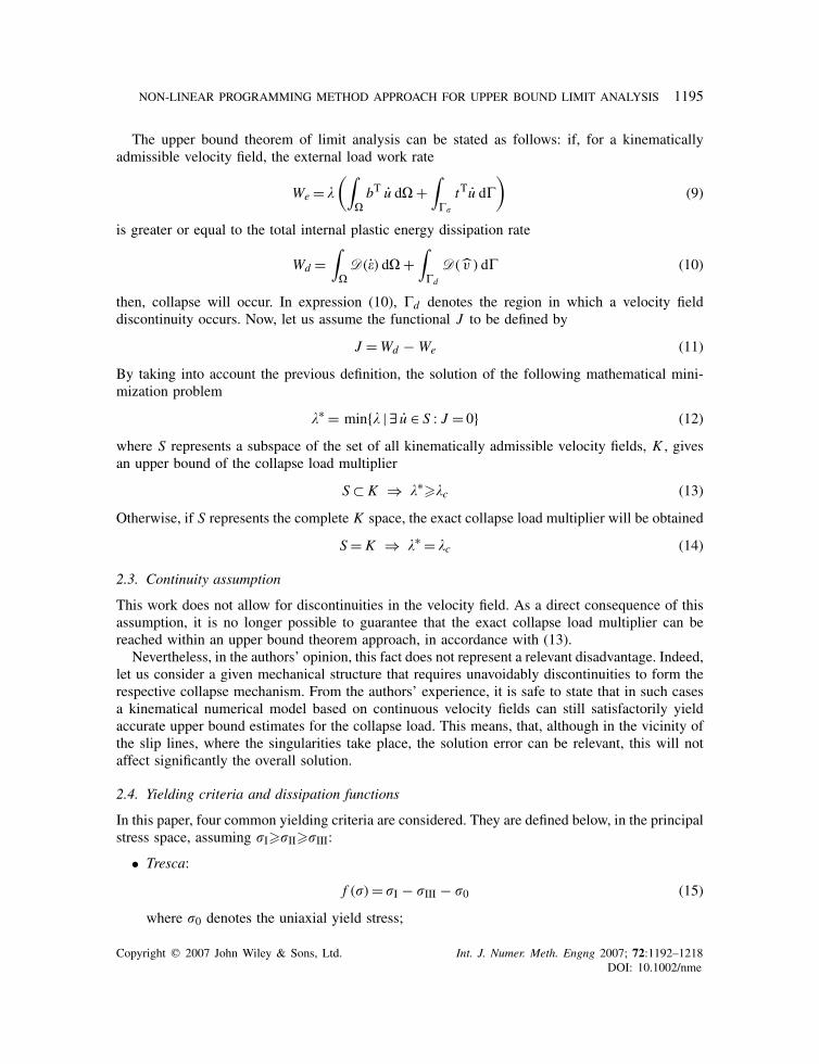
The upper bound theorem of limit analysis can be stated as follows: if, for a kinematicallyadmissible velocity field, the external load work rate

We = �

(∫�bT u d� +

∫��

tTu d�

)(9)

is greater or equal to the total internal plastic energy dissipation rate

Wd =∫

�D(�) d� +

∫�d

D( v ) d� (10)

then, collapse will occur. In expression (10), �d denotes the region in which a velocity fielddiscontinuity occurs. Now, let us assume the functional J to be defined by

J =Wd − We (11)

By taking into account the previous definition, the solution of the following mathematical mini-mization problem

�∗ = min{� | ∃ u ∈ S : J = 0} (12)

where S represents a subspace of the set of all kinematically admissible velocity fields, K , givesan upper bound of the collapse load multiplier

S ⊂ K ⇒ �∗��c (13)

Otherwise, if S represents the complete K space, the exact collapse load multiplier will be obtained

S = K ⇒ �∗ = �c (14)

2.3. Continuity assumption

This work does not allow for discontinuities in the velocity field. As a direct consequence of thisassumption, it is no longer possible to guarantee that the exact collapse load multiplier can bereached within an upper bound theorem approach, in accordance with (13).

Nevertheless, in the authors’ opinion, this fact does not represent a relevant disadvantage. Indeed,let us consider a given mechanical structure that requires unavoidably discontinuities to form therespective collapse mechanism. From the authors’ experience, it is safe to state that in such casesa kinematical numerical model based on continuous velocity fields can still satisfactorily yieldaccurate upper bound estimates for the collapse load. This means, that, although in the vicinity ofthe slip lines, where the singularities take place, the solution error can be relevant, this will notaffect significantly the overall solution.

2.4. Yielding criteria and dissipation functions

In this paper, four common yielding criteria are considered. They are defined below, in the principalstress space, assuming �I��II��III:

• Tresca:

f (�) = �I − �III − �0 (15)

where �0 denotes the uniaxial yield stress;

Copyright q 2007 John Wiley & Sons, Ltd. Int. J. Numer. Meth. Engng 2007; 72:1192–1218DOI: 10.1002/nme

1196 M. VICENTE DA SILVA AND A. N. ANTAO

Table I. Plastic energy dissipation rate functions.

Criteria D(�) �∈Cc

Tresca �02 (|�I| + |�II| + |�III|)

tr(�) = 0

von Mises k√2 tr(�2)

Mohr–Coulomb tr(�)�(|�I| + |�II| + |�III|) sin�c

tan� tr(�)Drucker–Prager tr(�)�

√2 sin2 �

3+sin2 �(3 tr(�2) − tr2(�))

• von Mises:

f (�) =√

12 tr(s

2) − k (16)

where s represents the deviatoric stress, k the pure shear yield stress and tr(·) denotes thetrace tensorial operation;

• Mohr–Coulomb:f (�) = �I(1 + sin�) − �III(1 − sin�) − 2c cos� (17)

where c represents the cohesion and � the angle of shearing resistance;• Drucker–Prager:

f (�) =√1

2tr(s2) − 3 sin�√

3(3 + sin2 �)

(c

tan�− 1

3tr(�)

)(18)

Table I summarizes the internal energy dissipation functions together with the respective Ccspace definition, for all the previously mentioned yielding criteria. These expressions are presentedonly for the continuous strain rate condition.

3. NUMERICAL FORMULATION

As a starting point, let us divide the domain, �, into nE finite elements. For each element, twoindependent and simultaneous approximations, for the velocity and plastic strain rate fields, are used

ui = {vx , vy, vz}Ti = Nidi in �i (19)

�i = {�x , �y, �z, 2�xy, 2�yz, 2�xz}Ti = Eiei in �i (20)

The matrices N and E collect the approximation functions and the vectors d and e theirassociated weights, in reference to the i th finite element. For simplicity, the notation used in thissection assumes the 3D problem form. The adjustments needed for other types of problems arestraightforward.

The velocity approximation functions used are the conventional nodal shape functions from thefinite element method, FEM [11]. Thus, continuity in velocity field solution is imposed. As another

Copyright q 2007 John Wiley & Sons, Ltd. Int. J. Numer. Meth. Engng 2007; 72:1192–1218DOI: 10.1002/nme

NON-LINEAR PROGRAMMING METHOD APPROACH FOR UPPER BOUND LIMIT ANALYSIS 1197

YES

YES

NO

NO

Exit=

INITIALIZATION: R : R c

L : L c

SolveProblem (21)

Wd We ?

R =

L =

= R + L

2

”stop criterion”reached ?λ λ

λ λ

λλ

λλ λ

λλλ

λλλ

∗

Figure 1. Optimal collapse load search algorithm.

consequence of this field approximation, subspace S only fulfills condition (13) and condition (14)is no longer valid. Regarding the approximation of the plastic strain rate field, local functions areconsidered for each finite element, without any relation with the adjacent elements.

In order to solve the mathematical programming problem (12), the following strategy isadopted:

• for a given load multiplier, �, an optimal continuous kinematic field which minimizes thedifference between dissipated and external work rate, J , is searched

Min J

s.t. � = Bu

� ∈Cc

(21)

Since velocity and strain rate fields are independently approximated, the relationship betweenthese two fields is established as a constraint in problem (21);

• following the kinematical theorem, if, for the optimal solution of (21), J value is non-positive,� will unavoidably be an upper bound of the collapse load parameter (���c). Otherwise, noconclusions can be drawn.

Therefore, the search for the best collapse load multiplier can be achieved by a simple iterativealgorithm, as shown in Figure 1. The authors have improved the efficiency of the describedalgorithm with a few small adjustments. In fact, when the size of the search interval for thecollapse load multiplier is smaller than a given threshold, the search for �∗ is carried out usingalgorithm 2 (Figure 2).

3.1. Mathematical programming problem

This section presents the method to solve the minimization problem (21). First, the augmentedLagrangian method [12] is applied to (21), thus producing the following velocity field minimization

Copyright q 2007 John Wiley & Sons, Ltd. Int. J. Numer. Meth. Engng 2007; 72:1192–1218DOI: 10.1002/nme

1198 M. VICENTE DA SILVA AND A. N. ANTAO

YES

YES

NO

NO

Exit=

INITIALIZATION: s = R L

2

SolveProblem (21)

Wd We ?

R =

s =s

2

= R s

”stop criterion”reached ?

λλ

λ λ

λλ

λλ∗

Figure 2. Optimal collapse load search algorithm 2.

problem:

Min�∈Cc

L(u, �, �) =∫

�D(�) d� − �

(∫�bTu d� +

∫��

tTu d�

)

+∫

�� : (Bu − �) d� + r

2

∫�

‖Bu − �‖2 d� (22)

where the � vector collects the Lagrange multipliers and r denotes the penalty parameter, a positivescalar. In Equation (22), the first two terms are the J functional, where the discontinuity velocityterm in the dissipated energy rate expression is cancelled out, since it is discarded by the finiteelement formulation. The last two terms introduce the compatibility constraint (8), present inproblem (21), in the objective function.

Now, taking into consideration the finite element discretization of the domain and the fieldapproximations (19)–(20), the augmented Lagrangian definition is re-written in the followingexpanded way:

L(d, e, �) =nE∑i=1

∫�i

D(Eiei ) d� − �nE∑i=1

(∫�i

bTNi d� +∫

��i

tTNi d�

)di

+nE∑i=1

∫�i

�Ti A0(BNi ) d�di −nE∑i=1

∫�i

�Ti A0Eiei d�

+ r

2

nE∑i=1

dTi

∫�i

(BNi )TA0(BNi ) d�di − r

nE∑i=1

dTi

∫�i

(BNi )TA0(Eiei ) d�

+ r

2

nE∑i=1

∫�i

(Eiei )TA0(Eiei ) d� (23)

Copyright q 2007 John Wiley & Sons, Ltd. Int. J. Numer. Meth. Engng 2007; 72:1192–1218DOI: 10.1002/nme

NON-LINEAR PROGRAMMING METHOD APPROACH FOR UPPER BOUND LIMIT ANALYSIS 1199

YES

YES

NO

NO

INITIALIZATION:

STEP 1:

STEP 2:

”stop criterion”reached ?

EXIT

k = 0 , m = 0;vectors µ k and ek,m

are arbitrary chosen

m = m + 1;with µk and ek,m 1:

Min (dk,m )

with µ k and dk,m :Min (ek,m )

number of theadopted m cycles

reached ?

µ k+ 1i = µ k

i + B Ni dk,mi Ei e

k,mi )

ek+ 1,0 = ek,m

k = k + 1 , m = 0

�

Figure 3. Uzawa’s algorithm.

where the differential operator, B, the Lagrange multipliers vector, �, and the A0 matrix, assumethe form:

B =

⎡⎢⎢⎢⎢⎢⎢⎢⎢⎢⎢⎢⎢⎢⎢⎢⎢⎢⎢⎢⎢⎢⎢⎢⎣

��x

· ·

· ��y

·

· · ��z

��y

��x

·

· ��z

��y

��z

· ��x

⎤⎥⎥⎥⎥⎥⎥⎥⎥⎥⎥⎥⎥⎥⎥⎥⎥⎥⎥⎥⎥⎥⎥⎥⎦

, �i =

⎧⎪⎪⎪⎪⎪⎪⎪⎪⎪⎪⎨⎪⎪⎪⎪⎪⎪⎪⎪⎪⎪⎩

�x

�y

�z

2�xy

2�yz

2�xz

⎫⎪⎪⎪⎪⎪⎪⎪⎪⎪⎪⎬⎪⎪⎪⎪⎪⎪⎪⎪⎪⎪⎭i

, A0 =

⎡⎢⎢⎢⎢⎢⎢⎢⎢⎢⎢⎣

1 · · · · ·· 1 · · · ·· · 1 · · ·· · · 1

2 · ·· · · · 1

2 ·· · · · · 1

2

⎤⎥⎥⎥⎥⎥⎥⎥⎥⎥⎥⎦

To perform the minimization of the Langrangian (23), Uzawa’s iterative saddle-point searchalgorithm can be used [13]. Figure 3 summarizes Uzawa’s algorithm.

This algorithm displays quite a robust convergence, which is ensured whenever the number ofinner iterations, m, is higher or equal to 1 (m = 3 was adopted) and the value of � belongs tothe [0, 2r ] interval (�= r was adopted). A fully detailed explanation of Uzawa’s method and itsconvergence properties can be found in Reference [13].

Two independent minimizations must be carried out to perform Uzawa’s algorithm. The firstoccurs during STEP 1, with respect to the nodal displacements and affects all the elementssimultaneously. This minimization is straightforward. For variable d , the Lagrangian (23) is an

Copyright q 2007 John Wiley & Sons, Ltd. Int. J. Numer. Meth. Engng 2007; 72:1192–1218DOI: 10.1002/nme

1200 M. VICENTE DA SILVA AND A. N. ANTAO

unconstrained quadratic function. Thus, the minimizer is obtained by

�L(d, e, �)

�d= −�

nE∑i=1

(∫�i

bTNi d� +∫

��i

tTNi d�

)+

nE∑i=1

∫�i

�Ti A0(BNi ) d� + rnE∑i=1

∫�i

(BNi )TA0(BNi ) d�di

− rnE∑i=1

∫�i

(BNi )TA0(Eiei ) d�= 0 (24)

The result is a linear system of equations, which must be solved for each iteration. It can beexpressed in the following matrix form:

[A]{d}k,m = �{F} − {�}k + {L}k,m−1 (25)

where,

[A] = rnE∑i=1

∫�i

(BNi )TA0(BNi ) d� (26a)

{F} =nE∑i=1

(∫�i

bTNi d� +∫

��i

tTNi d�

)(26b)

{�}k =nE∑i=1

∫�i

(BNi )TA0(�i )

k d� (26c)

{L}k,m−1 = rnE∑i=1

∫�i

(BNi )TA0(Eiei )

k,m−1 d� (26d)

Of note is the fact that the computational procedures of all the terms present in the governingsystem are, in all aspects, similar to the ones adopted for the FEM.

The second minimization takes place during STEP 2 of Uzawa’s algorithm. In this stage, dueto the definitions of the functions of plastic energy dissipation, D (summarized in Table I), thenon-linearity of the problem emerges, which increases its complexity. However, the difficultiesthat arise from the minimization problem are confined to each finite element, by the adoptedplastic strain approximation (20). In fact, it will be shown that this minimization can be solvedindividually, element by element.

3.2. Local minimization

By assuming variables d and � as fixed throughout the local minimization process for variable ein every (k,m) iteration, the objective function (23) can be simplified for each finite element:

L∗i (ei ) =

∫�i

D(Eiei ) d� −∫

�i

�Ti A0Eiei d�

− r∫

�i

(BNidi )TA0(Eiei ) d� + r

2

∫�i

(Eiei )TA0(Eiei ) d� (27)

where, for notational simplicity, the k,m iteration superscripts were dropped out.

Copyright q 2007 John Wiley & Sons, Ltd. Int. J. Numer. Meth. Engng 2007; 72:1192–1218DOI: 10.1002/nme

NON-LINEAR PROGRAMMING METHOD APPROACH FOR UPPER BOUND LIMIT ANALYSIS 1201

Let us now assume that the strain approximation functions matrix, Ei , is the identity matrix.This assumption has important consequences: (i) the strain rate field is constant for each elementof the domain; (ii) e vector components gain a direct physical meaning as they represent the strainrate tensor components; (iii) the integrations in the above expression can be eliminated withoutaffecting the optimality point

L∗i (ei ) =D(ei ) − sTA0 ei + r

2eTi A0ei (28)

where

si = {sx , sy, sz, 2sxy, 2syz, 2szx }Ti = �i + r BNidi (29)

(iv) to ensure final solution compatibility, the velocity approximation functions will be linear;therefore, 3-node triangle and 4-node tetrahedral isoparametric elements are used for 2D planestrain and 3D solid problems, respectively.

Mention must be made of the fact that at this stage of development it is not yet possible to extendthe implementation of the model to higher order elements (i.e. elements with non-constant strainrate approximations), if a strict upper bound policy is required. The first obstacle is to impose thenormality flow rule restriction to all the element domain (�∈Cc). For linear strain elements, asshown in the work of Makrodimopoulos and Martin [14], this difficulty can, however, be overcomeby imposing the normality rule on the element vertices. The second obstacle results from the factthat the mathematical complexity of the optimization subproblem (27) increases. In this case, theapproach presented here to solve this minimization is no longer suitable, a procedure with provenefficiency has not been found so far.

A final step can be made to simplify the local minimization problem. According to Le Tallec[15], a new equivalent minimization problem, formulated in the principal strain space, can bederived and expressed as follows:

Minei∈C

L∗i (ei ) =D(ei ) − sTi ei + r

2eTi ei (30)

where vector, ei ={eI, eII, eIII}Ti , collects the principal components of the domain strain rate tensorapproximation, and vector si gathers the Si matrix eigenvalues, which are sorted in decreasingorder (sI�sII�sIII). The matrix Si is defined by

Si =

⎡⎢⎢⎣sx sxy szx

sxy sy syz

szx syz sz

⎤⎥⎥⎦i

(31)

Of note is the fact that the first and last terms from the objective function (30) present an isotropicbehaviour. On the contrary, for the middle term, each strain rate component is affected differentlyby the coefficients of si vector. Therefore, it is possible to conclude, by taking into accountthe order adopted for these coefficients, that the optimal solution shares necessarily the samecharacteristic

eI�eII�eIII (32)

Copyright q 2007 John Wiley & Sons, Ltd. Int. J. Numer. Meth. Engng 2007; 72:1192–1218DOI: 10.1002/nme

1202 M. VICENTE DA SILVA AND A. N. ANTAO

Another relevant property, stated in [15], is the following matrix orthogonal decompositionrelationship: ⎡⎢⎣

ex exy ezx

exy ey eyz

ezx eyz ez

⎤⎥⎦i

= Yi

⎡⎢⎣eI · ·· eII ·· · eIII

⎤⎥⎦i

Y Ti (33)

Here, matrix Yi collects, column-wise, the normalized eigenvectors of Si matrix sorted in the sameway as the eigenvalues.

The different procedures adopted to solve the minimization problem (30) are explained in detailin the Appendix, for the different yielding criteria.

3.3. Locking phenomenon

Tresca and von Mises criteria impose that plastic flow should occur under volumetric incompress-ibility conditions, by enforcing tr(�) = 0 in Equation (7). Therefore, the locking phenomenon canemerge. This is a well-known numerical problem of finite elements displacement formulations, as-sociated with incompressive kinematical behaviour, in which the solution becomes very inaccurateas a result of excessive stiffness of the model.

For Mohr–Coulomb and Drucker–Prager criteria, the admissible plastic strain domain (Cc) isdefined by a less or equal condition constraint which is less restrictive than the equality constraint,imposed by the isochoric materials. However, the inequality condition is restricted to plastic strainsdue to stress states located on the vertex of the yield surface. Thus, if the collapse problem understudy is governed by a compressive failure behaviour, the equality condition is always activatedand may affect the numerical results with a behaviour analogous to the volumetric locking, asshown in [16] for plane strain problems. Nevertheless, the authors avow from their experience thatthey never detected cases in which the results were manifestly affected by locking effects whenusing Mohr–Coulomb or Drucker–Prager materials.

In an attempt to overcome the locking problem, special geometric arrangements are used. Inthe case of 3-node triangle meshes, a very efficient distribution is proposed in Reference [17]:each set of four elements must form a quadrilateral with the central node in the intersection of thediagonals.

A similar procedure is adopted for 3D meshes: each assembly of 24 tetrahedrons must form ahexahedron with nodes positioned on every vertex; each face contains a middle node located in theintersection of the diagonals; finally, a central node is placed on the intersection of the diagonalsof vertices. However, of note is the fact that this 3D combination of elements does not guaranteethe elimination of the locking problem. To the best of our knowledge, no successful arrangementhas so far proven suitable for this type of elements.

4. ILLUSTRATIVE RESULTS

In order to illustrate the performance and versatility of the proposed method, different classes ofexamples were studied. Whenever possible, the results are compared either with analytical solutionsor with the outcome of other numerical formulations. All the results reported in this paper were

Copyright q 2007 John Wiley & Sons, Ltd. Int. J. Numer. Meth. Engng 2007; 72:1192–1218DOI: 10.1002/nme

NON-LINEAR PROGRAMMING METHOD APPROACH FOR UPPER BOUND LIMIT ANALYSIS 1203

2.5

5.0

5.05.0

7.5

8.0

8.0

4.0

F

N+y = 2N−

y 3D view(frontal view)

Collapse Mechanism

Figure 4. Strut-and-tie tower structure.

computed in a PC machine equipped with a Pentium IV 2.4GHz CPU and a 1.0GB RAM. Thequadrilateral and hexahedral base meshes were generated using TrueGrid [18] software.

4.1. Strut-and-tie 3D structure

In this example, the plastic load of collapse of a strut-and-tie tower structure is computed. Thetower, represented in Figure 4, consists of 114 bars and is subject to three concentrated loads atthe top level. The yielding tension capacity, N+

y , is the same for all bars and is the double of thevalue of the yielding compression capacity (N+

y = 2N−y ).

The practical interest of this type of problems is limited, given that the bearing capacity ofsuch structures is constantly dictated by instability phenomenon. Nevertheless, the 2-node barelement was implemented by taking into consideration its utility when conjugated with 2D and3D elements.

This simple example was chosen not only to fully demonstrate the versatility of the proposedmethod, but also because, in this particular case, the finite element velocity approximation enclosesall the kinematic admissible fields, i.e. condition (14) is verified. Thus, the exact collapse loadis likely to be reached. As predicted, the exact collapse load, F � 0.97742N+

y , was reached in0.45 s. Figure 4 shows the attained collapse mechanism.

4.2. Prandtl’s punch problem

As a plane strain example, we study the classical Prandtl’s punch problem, which is represented inFigure 5. The strong discontinuity at the footing edge makes this problem numerically demanding.It places a challenge to the present method, which does not contemplate discontinuities in thevelocity field.

First, the analysis of Tresca material was performed for two cases: (a) a rigid rough footingand (b) a perfectly flexible footing. The footing deformability does not alter the upper boundapproximation of the collapse load value, which is in accordance with Prandtl’s analytical solution

Copyright q 2007 John Wiley & Sons, Ltd. Int. J. Numer. Meth. Engng 2007; 72:1192–1218DOI: 10.1002/nme

1204 M. VICENTE DA SILVA AND A. N. ANTAO

p

L

bH

Figure 5. Prandtl’s punch problem: model geometry.

Table II. Prandtl’s punch problem for Tresca material:comparison of solutions by different methods.

Authors and methods Scaled collapse load Time (s)

Analytical [19] 2 + �� 5.142 —Present work (b) 5.170 52Tin-Loi and Ngo [20] 5.173 —Capsoni [21] 5.191 —Sloan and Kleeman [1] 5.210 —Capsoni and Corradi [22] 5.240 —Present work (a) 5.264 57

[19]. A mesh of 4784 3-node elements was used to discretize the domain, defined for H = 2b andL = 4b. In an attempt to overcome the singularity caused by the footing extremity, the mesh densitywas increased below that region. Table II presents, using the dimensionless parameter 2p/�0, thecollapse loads obtained and the respective CPU times. The results proved to be competitive withother methods and showed a very good accuracy when compared with the analytical solution.As expected, it is in case (a), in which the footing rigidity imposes a stronger singularity, thatthe larger discrepancy with the exact solution is observed. Even so, the error in this case did notexceed 2.4%. Better results can be attained by increasing the number of finite elements, sincethese analyses only required about 5% of the available memory and a reduced CPU time. In fact,a more refined mesh using 28 212{38 572} elements was tested for the rigid footing scenario anda value of 5.204{5.198} was attained for the upper bound estimated value, which corresponds toa 1.21%{1.10%} error value. The CPU time in this case was 405{684} s.

Figure 6 illustrates the distribution of the plastic dissipation energy rate of collapse (normalizedto the maximum value) and the respective collapse mechanisms. These dissipation patterns clearlyindicate that the two cases under study form different punch mechanisms. In case (a), the mechanismis similar to the one proposed by Prandtl [19], with a single large rigid block under the footing.Case (b) presents a more similar mechanism with the one proposed by Hill [23]. Another differencebetween the two solutions is the fact that in case (a) the plastic dissipation is more concentratedon narrower regions, approaching the form of well-defined slip lines.

The punch collapse load problem is also analysed using Mohr–Coulomb material with differentshearing resistance angles (�), considering only the perfectly flexible footing case. The resultsare juxtaposed with the analytical curve [19] in the graph of Figure 7. Once more, the resultsmatch the exact solution perfectly. The error never exceeds 1.87%. The highest CPU time of

Copyright q 2007 John Wiley & Sons, Ltd. Int. J. Numer. Meth. Engng 2007; 72:1192–1218DOI: 10.1002/nme

NON-LINEAR PROGRAMMING METHOD APPROACH FOR UPPER BOUND LIMIT ANALYSIS 1205

Dis

sipa

tion

Vel

ocity

mag

nitu

de

|0.20

0.15

0.10

0.05

0.00

(a)

(b)

v|| max

0

Figure 6. Prandtl’s punch problem: plastic dissipation energy rate and collapse mechanism: (a) rigidfooting and (b) flexible footing.

0.55% 0.88% 0.77% 0.61%0.80%

1.11%1.16%

1.09%

1.51%

1.87%

00 5 10 15

20

20 25 30 35

40

40 45

60

80

100

120

140

Upper bound

Analytical

Sca

led

co

llap

se l

oad

(p c

)

Angle of shearing resistance φ

Figure 7. Punch problem: scaled collapse load and relative error for Mohr–Coulomb material.

487 s and available memory use of 22% occurred during the computations for a � value of 35◦and 45◦, respectively. The increase in � value expands the region of the collapse mechanisms.Therefore, the analysis domain had to be amplified for higher values of �, which required the useof more finite elements to maintain the level of accuracy. This procedure justifies the increasinguse of computational resources when compared with the ones used during the analysis with Tresca

Copyright q 2007 John Wiley & Sons, Ltd. Int. J. Numer. Meth. Engng 2007; 72:1192–1218DOI: 10.1002/nme

1206 M. VICENTE DA SILVA AND A. N. ANTAO

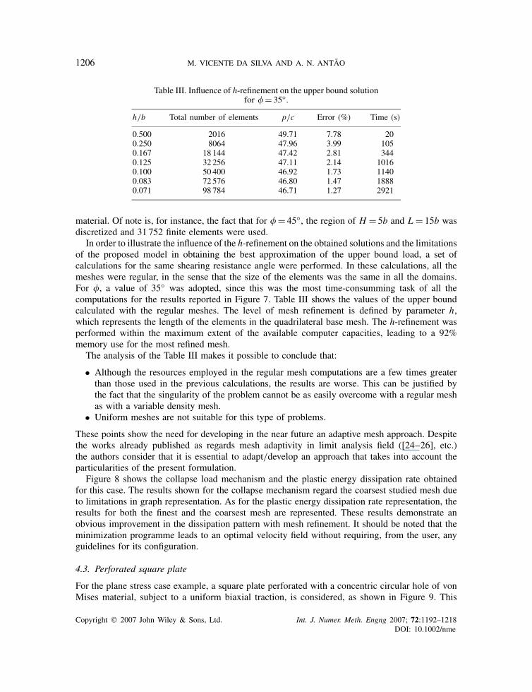
Table III. Influence of h-refinement on the upper bound solutionfor � = 35◦.

h/b Total number of elements p/c Error (%) Time (s)

0.500 2016 49.71 7.78 200.250 8064 47.96 3.99 1050.167 18 144 47.42 2.81 3440.125 32 256 47.11 2.14 10160.100 50 400 46.92 1.73 11400.083 72 576 46.80 1.47 18880.071 98 784 46.71 1.27 2921

material. Of note is, for instance, the fact that for �= 45◦, the region of H = 5b and L = 15b wasdiscretized and 31 752 finite elements were used.

In order to illustrate the influence of the h-refinement on the obtained solutions and the limitationsof the proposed model in obtaining the best approximation of the upper bound load, a set ofcalculations for the same shearing resistance angle were performed. In these calculations, all themeshes were regular, in the sense that the size of the elements was the same in all the domains.For �, a value of 35◦ was adopted, since this was the most time-consumming task of all thecomputations for the results reported in Figure 7. Table III shows the values of the upper boundcalculated with the regular meshes. The level of mesh refinement is defined by parameter h,which represents the length of the elements in the quadrilateral base mesh. The h-refinement wasperformed within the maximum extent of the available computer capacities, leading to a 92%memory use for the most refined mesh.

The analysis of the Table III makes it possible to conclude that:

• Although the resources employed in the regular mesh computations are a few times greaterthan those used in the previous calculations, the results are worse. This can be justified bythe fact that the singularity of the problem cannot be as easily overcome with a regular meshas with a variable density mesh.

• Uniform meshes are not suitable for this type of problems.

These points show the need for developing in the near future an adaptive mesh approach. Despitethe works already published as regards mesh adaptivity in limit analysis field ([24–26], etc.)the authors consider that it is essential to adapt/develop an approach that takes into account theparticularities of the present formulation.

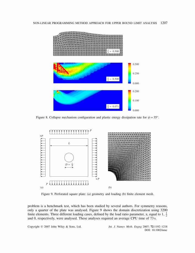
Figure 8 shows the collapse load mechanism and the plastic energy dissipation rate obtainedfor this case. The results shown for the collapse mechanism regard the coarsest studied mesh dueto limitations in graph representation. As for the plastic energy dissipation rate representation, theresults for both the finest and the coarsest mesh are represented. These results demonstrate anobvious improvement in the dissipation pattern with mesh refinement. It should be noted that theminimization programme leads to an optimal velocity field without requiring, from the user, anyguidelines for its configuration.

4.3. Perforated square plate

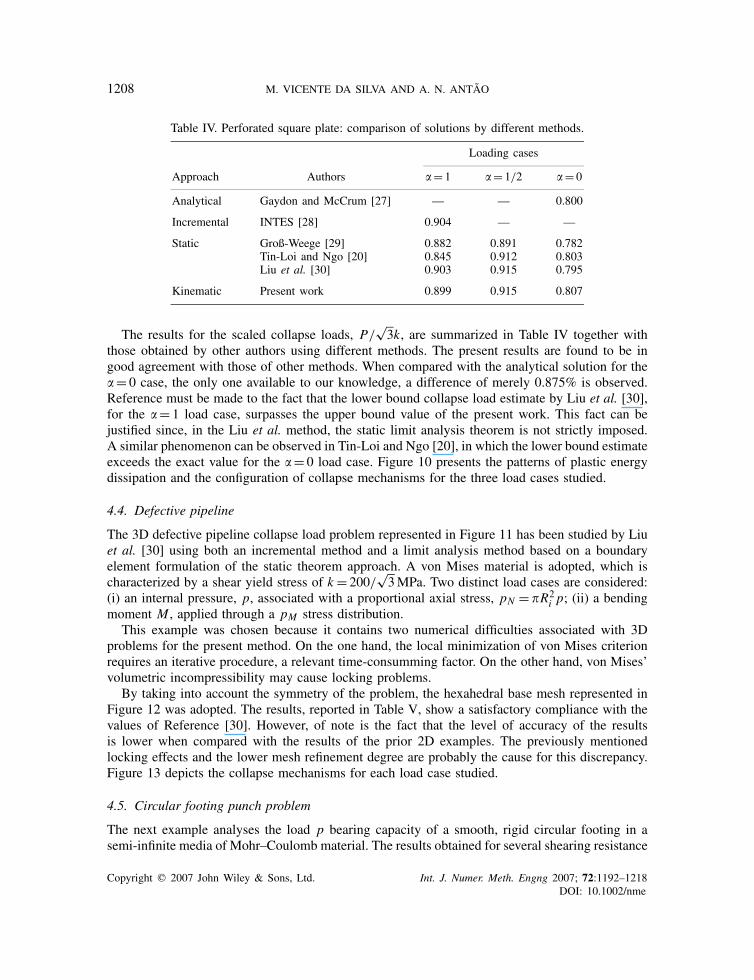
For the plane stress case example, a square plate perforated with a concentric circular hole of vonMises material, subject to a uniform biaxial traction, is considered, as shown in Figure 9. This

Copyright q 2007 John Wiley & Sons, Ltd. Int. J. Numer. Meth. Engng 2007; 72:1192–1218DOI: 10.1002/nme

NON-LINEAR PROGRAMMING METHOD APPROACH FOR UPPER BOUND LIMIT ANALYSIS 1207

hb = 0.500

hb = 0.500

hb = 0.071

0.000

0.000

0.250

0.500

0.100

0.200

Figure 8. Collapse mechanism configuration and plastic energy dissipation rate for � = 35◦.

P

P

P

P

L

D = L5

�

�

(a) (b)

Figure 9. Perforated square plate: (a) geometry and loading (b) finite element mesh.

problem is a benchmark test, which has been studied by several authors. For symmetry reasons,only a quarter of the plate was analysed. Figure 9 shows the domain discretization using 3200finite elements. Three different loading cases, defined by the load ratio parameter, �, equal to 1, 1

2and 0, respectively, were analysed. These analyses required an average CPU time of 73 s.

Copyright q 2007 John Wiley & Sons, Ltd. Int. J. Numer. Meth. Engng 2007; 72:1192–1218DOI: 10.1002/nme

1208 M. VICENTE DA SILVA AND A. N. ANTAO

Table IV. Perforated square plate: comparison of solutions by different methods.

Loading cases

Approach Authors �= 1 �= 1/2 �= 0

Analytical Gaydon and McCrum [27] — — 0.800

Incremental INTES [28] 0.904 — —

Static Groß-Weege [29] 0.882 0.891 0.782Tin-Loi and Ngo [20] 0.845 0.912 0.803Liu et al. [30] 0.903 0.915 0.795

Kinematic Present work 0.899 0.915 0.807

The results for the scaled collapse loads, P/√3k, are summarized in Table IV together with

those obtained by other authors using different methods. The present results are found to be ingood agreement with those of other methods. When compared with the analytical solution for the� = 0 case, the only one available to our knowledge, a difference of merely 0.875% is observed.Reference must be made to the fact that the lower bound collapse load estimate by Liu et al. [30],for the � = 1 load case, surpasses the upper bound value of the present work. This fact can bejustified since, in the Liu et al. method, the static limit analysis theorem is not strictly imposed.A similar phenomenon can be observed in Tin-Loi and Ngo [20], in which the lower bound estimateexceeds the exact value for the � = 0 load case. Figure 10 presents the patterns of plastic energydissipation and the configuration of collapse mechanisms for the three load cases studied.

4.4. Defective pipeline

The 3D defective pipeline collapse load problem represented in Figure 11 has been studied by Liuet al. [30] using both an incremental method and a limit analysis method based on a boundaryelement formulation of the static theorem approach. A von Mises material is adopted, which ischaracterized by a shear yield stress of k = 200/

√3MPa. Two distinct load cases are considered:

(i) an internal pressure, p, associated with a proportional axial stress, pN = �R2i p; (ii) a bending

moment M , applied through a pM stress distribution.This example was chosen because it contains two numerical difficulties associated with 3D

problems for the present method. On the one hand, the local minimization of von Mises criterionrequires an iterative procedure, a relevant time-consumming factor. On the other hand, von Mises’volumetric incompressibility may cause locking problems.

By taking into account the symmetry of the problem, the hexahedral base mesh represented inFigure 12 was adopted. The results, reported in Table V, show a satisfactory compliance with thevalues of Reference [30]. However, of note is the fact that the level of accuracy of the resultsis lower when compared with the results of the prior 2D examples. The previously mentionedlocking effects and the lower mesh refinement degree are probably the cause for this discrepancy.Figure 13 depicts the collapse mechanisms for each load case studied.

4.5. Circular footing punch problem

The next example analyses the load p bearing capacity of a smooth, rigid circular footing in asemi-infinite media of Mohr–Coulomb material. The results obtained for several shearing resistance

Copyright q 2007 John Wiley & Sons, Ltd. Int. J. Numer. Meth. Engng 2007; 72:1192–1218DOI: 10.1002/nme

NON-LINEAR PROGRAMMING METHOD APPROACH FOR UPPER BOUND LIMIT ANALYSIS 1209

Figure 10. Plastic dissipation pattern and collapse mechanisms configurations.

Re = 70

Ri = 50

60

30

120

pN

p

p

pM

N

M

18o

Figure 11. Defective pipeline.

angles (�) are presented in Table VI and compared with the exact solution derived by Cox et al.[31]. The same table also shows the values computed by an accurate lower bound method proposedby Lyamin and Sloan [6].

By taking into consideration the axisymmetry of the problem, only a 5◦ slice was studied, usingmeshes of a fixed number of 45 541 tetrahedral finite elements. This number of elements required36% of the available memory. The length and depth of the meshes were adjusted according to

Copyright q 2007 John Wiley & Sons, Ltd. Int. J. Numer. Meth. Engng 2007; 72:1192–1218DOI: 10.1002/nme

1210 M. VICENTE DA SILVA AND A. N. ANTAO

Figure 12. Defective pipeline: hexahedral base mesh.

Table V. Defective pipeline: comparison of solutions by different methods.

Case a Case b

Approach Authors Collapse pressure (MPa) Time (s) Collapse moment (kNm) Time (s)

Kinematic Present work 67.13 697 56.02 611Incremental Liu et al. [30] 64.05 — 55.27 —Static Liu et al. [30] 63.42 — 54.96 —

load case (ii)load case (i)

Figure 13. Defective pipeline: configurations of the collapse mechanisms.

angle �. As in the Prandtl punch problem, the singularities at the edge of the footing pose anumerical constraint to the present method. In order to overcome this problem, the mesh elementswere refined in this region.

For the friction angle of �= 40◦, the colapse load obtained showed that the originally adoptedmesh was not able to produce satisfactory results. Therefore, a new mesh of 52 981 elements was

Copyright q 2007 John Wiley & Sons, Ltd. Int. J. Numer. Meth. Engng 2007; 72:1192–1218DOI: 10.1002/nme

NON-LINEAR PROGRAMMING METHOD APPROACH FOR UPPER BOUND LIMIT ANALYSIS 1211

Table VI. Circular footing punch problem: comparison of solutions by different methods.

Upper bound (present work) Analytical [31] Lower bound [6]� (deg.) p/c Error (%) Time (s) p/c p/c Error (%)

0 5.80 +1.93 1102 5.69 5.54 −2.645 7.60 +2.15 1063 7.44 7.2 −3.23

10 10.26 +2.81 1085 9.98 9.61 −3.7115 14.34 +3.17 1081 13.9 13.3 −4.3220 20.80 +3.48 1266 20.1 19.06 −5.1730 51.9 +5.27 1696 49.3 — —

180.6 +10.12 160140 164 — —

174.4∗ +6.34∗ 2176∗

0.000 0.025 0.050 0.750 0.100

Figure 14. Scaled plastic dissipation energy rate for � = 15◦.

analysed. The collapse load obtained for this second mesh is presented in Table VI marked witha star (∗). The upper bounds predicted by the present method can be considered very accuratefor this type of problems. The computational costs are significant, but acceptable for this level ofaccuracy in this kind of problems. Figure 14 shows the plastic dissipation energy rate for � = 15◦,scaled to the maximum obtained value.

4.6. Conic excavation stability

Lastly, to conclude the example section, the stability of a conical excavation subject to its self-weight, , is analysed. The depth and the diameter at the base of the excavation correspond to 5and 2m, respectively. In order to simulate the soil behaviour, a cohesive-frictional material wasassumed, with a cohesion of c= 1 kPa and a friction angle of �= 20◦, using both Mohr–Coulomband Ducker–Prager criteria.

The results obtained for a range of slope angles, , are summarized in Table VII and comparedwith the solutions obtained with a discontinuous upper bound formulation [32]. Once more, theaxisymmetry of the problem was taken into account: only a 15◦ slice was discretized with theproper symmetry boundary conditions. In all the meshes adopted during the analyses of the differentslope angle excavations, a fixed number of 24 468 elements was used. This discretization resultsin a total of 181 456 problem unknowns, embodied by 17 324 and 164 132 degrees of freedomfor the velocity and strain rate field, respectively. For this same problem, a total of 325 206

Copyright q 2007 John Wiley & Sons, Ltd. Int. J. Numer. Meth. Engng 2007; 72:1192–1218DOI: 10.1002/nme

1212 M. VICENTE DA SILVA AND A. N. ANTAO

Table VII. Conic excavation stability: upper bound values and CPU time.

Present method Discontinuous formulation [32]Mohr–Coulomb Drucker–Prager Mohr–Coulomb Drucker–Prager

(deg.) H/c Time (s) H/c Time (s) H/c Time (s) H/c Time (s)

50 27.73 443 25.63 447 27.72 3120 25.75 53260 22.27 483 20.79 485 22.34 2700 20.80 48670 19.22 318 17.99 384 19.25 2580 18.06 44380 17.71 539 16.50 431 17.55 2280 16.52 378

0.0 0.175 0.350 0.525 0.7000.000|v|max

DissipationVelocity magnitude

Figure 15. Collapse load mechanism and scaled plastic dissipation energy rate for = 60◦.

problem unknowns were required to obtain the solutions reported by Krabbenhøft et al. [32], usedas reference. Mention must be made of the fact that the analysis in [32] was performed in anarchitecture about 1.4× slower than the one used to compute the results for the current work.

The results reveal not only a good agreement with those of [32], but also with the upper andlower bound estimates produced by different formulations, also mentioned in the paper referred toabove. Taken as a whole, the results show a better accuracy when compared with the upper boundreference values, and even for the worse result obtained the relative error never exceeds 0.9%.This fact supports the authors’ opinion, expressed in Section 2.3, that the continuity assumptiondoes not affect significantly the accuracy of the method and may represent a computational speedup. In fact, the authors consider that a discontinuous formulation would represent an advantageparticularly if conjugated with a proper adaptive mesh approach.

Another important feature of the present model, corroborated by these results, is its aptitude todeal with non-smooth yielding criteria without affecting the convergence rate of the method andconsequently the computational time.

Figure 15 shows the configuration of the collapse mechanism and the plastic energy dissipationrate for a slope angle excavation of 60◦, using Mohr–Coulomb criterion.

Copyright q 2007 John Wiley & Sons, Ltd. Int. J. Numer. Meth. Engng 2007; 72:1192–1218DOI: 10.1002/nme

NON-LINEAR PROGRAMMING METHOD APPROACH FOR UPPER BOUND LIMIT ANALYSIS 1213

5. CLOSURE

This paper implemented a finite element formulation using mathematical non-linear program-ming for computing collapse loads estimates and the respective failure mechanisms, based on thekinematical upper bound theorem of limit analysis.

Implementation and computational aspects were discussed for Tresca, von Mises,Mohr–Coulomb and Drucker–Prager yielding criteria. To perform domain space discretization,2-node bars, 3-node plane triangles and 4-node tetrahedral isoparametric elements were used. Toavoid or to diminish the locking phenomenon, particular geometric arrangements of finite elementswere used during mesh generation.

The efficiency, accuracy and robustness of the proposed method were demonstrated using somenumerical examples. The latter also demonstrate the versatility of the method that can be appliedto solve a wide range of collapse problems.

APPENDIX A: TRESCA MINIMIZATION CRITERION

A.1. 3D solid problems

As a starting point, the constraint of problem (30) is eliminated, by considering the definition ofCc (Table I) and the number of independent variables is reduced, using the following relationship:

eIII =−eI − eII (A1)

Introducing (A1) into the objective function, a R2 piecewise quadratic function is obtained

L∗(eI, eII) = �02

(|eI| + |eII| + |eI + eII|)

+ r(e2I + e2II + eIeII) + (sIII − sI)eI + (sIII − sII)eII (A2)

By taking into account condition (32), only four regions should be considered: eI = 0∧ eII = 0,eI>0∧ eII = 0, eI>0∧ eII>0 and eI>0∧ eII<0 the following points become thus feasible candidatesfor a minimizer:

e1 = {0, 0, eIII}T

e2 ={−�0 − sI + sIII

2r, 0, eIII

}T

e3 ={−�0 − 2sI + sII + sIII

3r, −�0 − 2sII + sI + sIII

3r, eIII

}T

e4 ={−2�0 − 2sI + sII + sIII

3r, −−�0 − 2sII + sI + sIII

3r, eIII

}T

(A3)

The most basic and yet efficient procedure to attain the minimizer is to test all these points andselect the best one.

Copyright q 2007 John Wiley & Sons, Ltd. Int. J. Numer. Meth. Engng 2007; 72:1192–1218DOI: 10.1002/nme

1214 M. VICENTE DA SILVA AND A. N. ANTAO

A.2. 2D plane strain problems

In this case, an extra and obvious condition is naturally imposed

eIII = 0 (A4)

and the feasible points are reduced to two

e1 = {0, 0}T

e2 ={−�0 + sI − sII

2r,�0 − sI + sII

2r

}T (A5)

APPENDIX B: VON MISES MINIMIZATION CRITERION

B.1. 3D solid problems

Similarly to the Tresca criterion, the constraint of the problem is eliminated and relationship (A1)is applicable. However, this time a non-linear objective function is obtained

L∗(eI, eII) = 2k√e2I + e2II + eIeII + r(e2I + e2II + eIeII) + (sIII − sI)eI + (sIII − sII)eII (B1)

To solve this unconstrained minimization problem, the Fletcher–Reeves algorithm [12] is used, asdescribed below. This algorithm is adapted from the conjugated gradient method and is suitablefor convex non-linear optimization. Each iteration step is obtained by

{eI, eII}Tk+1 = {eI, eII}Tk + �k pk, �k ∈ R+ (B2)

where �k is the step length and pk is the step direction

pk ={p1, p2}Tk =−∇L∗k + ∇L∗T

k ∇L∗k

∇L∗Tk−1∇L∗

k−1

pk−1 (B3)

The expression for the objective function gradient is given by

∇L∗(eI, eII) =

⎧⎪⎪⎪⎪⎪⎨⎪⎪⎪⎪⎪⎩

k(2eI + eII)√e2I + e2II + eIeII

+ r(2eI + eII) − sI + sIII

k(2eII + eI)√e2I + e2II + eIeII

+ r(2eII + eI) − sII + sIII

⎫⎪⎪⎪⎪⎪⎬⎪⎪⎪⎪⎪⎭(B4)

The best step length for k + 1 iteration can be accomplished by solving the following problem:

MinL∗k(eI + �p1, eII + �p2) (B5)

However, performing this exact minimization for every iteration is computationally very demanding.Instead, a good estimate is obtained by expanding this objective function in Taylor series (truncatedin the quadratic term) and by solving the resulting minimization problem analytically, thus deriving

Copyright q 2007 John Wiley & Sons, Ltd. Int. J. Numer. Meth. Engng 2007; 72:1192–1218DOI: 10.1002/nme

NON-LINEAR PROGRAMMING METHOD APPROACH FOR UPPER BOUND LIMIT ANALYSIS 1215

the next explicit formula

� = −⎡⎢⎣k(2eI p1 + 2eII p2 + eI p2 + eII p1)√

e2I + e2II + eIeII+ r(2eI p1 + 2eII p2 + eI p2 + eII p1)

− sI p1 − sII p2 + sIII(p1 + p2)

⎤⎥⎦/[3k(eI p2 − eII p1)2

2(e2I + eIeII + e2II)2/3

+ 2r(p21 + p22 + p1 p2)

](B6)

For notational simplicity, the k iteration superscript was dropped out. To start the algorithm, theinitial step direction is given by ∇L∗

0. A first reasonable guess of the solution is also needed.Prior simulations suggest as a good estimate the following point:

{eI

eII

}0

=

⎧⎪⎪⎨⎪⎪⎩2sI − sII − sIII

3(r + k)

2sII − sI − sIII3(r + k)

⎫⎪⎪⎬⎪⎪⎭ (B7)

B.2. 2D plane strain problems

For 2D plane strain problems, this criterion coincides with the Tresca criterion and, therefore, thesame optimization procedure can be used, with

√3k = �0.

APPENDIX C: MOHR–COULOMB MINIMIZATION CRITERION

C.1. 3D solid problems

A different strategy from the ones presented above is used to solve the Mohr–Coulomb criterionminimization. We now stand before a quadratic objective function, subject to piecewise linearinequality constraints.

Let us start by solving the problem regardless of constraints. In this case, the unconstrainedsolution, eu , is given by

eu ={o1, o2, o3}T = 1

r

{− c

tan(�)+ sI, − c

tan(�)+ sII, − c

tan(�)+ sIII

}T

(C1)

Subsequently, the previous solution is tested to check if it belongs to the feasible domain, eu ∈C.If so, the optimality point is reached. Otherwise, the solution consists in the closest point of theunconstrained optimal point, located on the feasible domain surface [33]

tr(�) =(|�I| + |�II| + |�III|) sin� (C2)

In fact, the coefficients affecting the quadratic terms of the objective function are the same (r/2).Therefore, the equipotential of the function surfaces define spheres centred on the unconstrainedoptimal point. Given that the feasible domain is convex, the optimal point is necessarily the point

Copyright q 2007 John Wiley & Sons, Ltd. Int. J. Numer. Meth. Engng 2007; 72:1192–1218DOI: 10.1002/nme

1216 M. VICENTE DA SILVA AND A. N. ANTAO

of the feasible domain nearest to the centre. According to restriction (32), only the following fourpoints are admissible candidates:

e1 = {0, 0, 0}T (C3a)

e2 =

⎧⎪⎪⎪⎪⎪⎨⎪⎪⎪⎪⎪⎩−(1 + sin(�))

(2H − sIII − sI) sin(�) − sI + sIII2r(sin(�)2 + 1)

0

− (2H − sIII − sI) sin(�)2 + 2(sIII − H) sin(�) + sI − sIII2r(sin(�)2 + 1)

⎫⎪⎪⎪⎪⎪⎬⎪⎪⎪⎪⎪⎭(C3b)

e3 =

⎧⎪⎪⎪⎪⎪⎪⎪⎨⎪⎪⎪⎪⎪⎪⎪⎩

o1 − (1 − sin(�))(1 − sin(�))o1 + (1 − sin(�))o2 + (1 + sin(�))o3

2(1 − sin(�))2 + (1 + sin(�))2

o2 − (1 − sin(�))(1 − sin(�))o1 + (1 − sin(�))o2 + (1 + sin(�))o3

2(1 − sin(�))2 + (1 + sin(�))2

o3 − (1 + sin(�))(1 − sin(�))o1 + (1 − sin(�))o2 + (1 + sin(�))o3

2(1 − sin(�))2 + (1 + sin(�))2

⎫⎪⎪⎪⎪⎪⎪⎪⎬⎪⎪⎪⎪⎪⎪⎪⎭(C3c)

e4 =

⎧⎪⎪⎪⎪⎪⎪⎪⎨⎪⎪⎪⎪⎪⎪⎪⎩

o1 − (1 − sin(�))(1 − sin(�))o1 + (1 + sin(�))o2 + (1 + sin(�))o3

(1 − sin(�))2 + 2(1 + sin(�))2

o2 − (1 + sin(�))(1 − sin(�))o1 + (1 + sin(�))o2 + (1 + sin(�))o3

(1 − sin(�))2 + 2(1 + sin(�))2

o3 − (1 + sin(�))(1 − sin(�))o1 + (1 + sin(�))o2 + (1 + sin(�))o3

(1 − sin(�))2 + 2(1 + sin(�))2

⎫⎪⎪⎪⎪⎪⎪⎪⎬⎪⎪⎪⎪⎪⎪⎪⎭(C3d)

Choosing the minimizer involves the following steps: (i) confirming if the points comply withEquation (C2); (ii) selecting, from among all the points that satisfy the previous condition, the onethat minimizes the objective function (30).

C.2. 2D plane strain problems

The same procedure can be applied to 2D plane strain problems. Taking into account condition(A4) the unconstrained solution, eu , is therefore given by

eu ={o1, o2}T = 1

r

{− c

tan(�)+ sI, − c

tan(�)+ sII

}T

(C4)

and the possible candidates located on the surface domain are reduced to two

e1 = {0, 0}T (C5a)

e2 =

⎧⎪⎪⎨⎪⎪⎩o1 − (1 − sin(�))

(1 − sin(�))o1 + (1 + sin(�))o2(1 − sin(�))2 + (1 + sin(�))2

o2 − (1 + sin(�))(1 − sin(�))o1 + (1 + sin(�))o2(1 − sin(�))2 + (1 + sin(�))2

⎫⎪⎪⎬⎪⎪⎭ (C5b)

A more detailed discussion about this minimization can be found in Reference [33].

Copyright q 2007 John Wiley & Sons, Ltd. Int. J. Numer. Meth. Engng 2007; 72:1192–1218DOI: 10.1002/nme

NON-LINEAR PROGRAMMING METHOD APPROACH FOR UPPER BOUND LIMIT ANALYSIS 1217

APPENDIX D: DRUCKER–PRAGER MINIMIZATION CRITERION

D.1. 3D solid problems

The local minimization for the Drucker–Prager criterion follows the same procedure adopted forthe Mohr–Coulomb criterion. However, the admissible candidates located on the feasible domainsurface, must be adjusted to comply with the Drucker–Prager criterion

tr(�)�

√2 sin2 �

3 + sin2 �(3 tr(�2) − tr2(�)) (D1)

hence, the points given by (C3a)–(C3d) are replaced by

e1 = {0, 0, 0}T (D2a)

e2 =

⎧⎪⎨⎪⎩w(−rm + 2sI − sII − sIII)

w(−rm + 2sII − sI − sIII)

w(−rm + 2sIII − sI − sII)

⎫⎪⎬⎪⎭ (D2b)

where

m = −1

r

√2 sin2(�)

3 + sin2(�)a, w =

rm

(3

c

tan(�)− sI − sII − sIII

)+ a

3r((rm)2 + a)

a = 2(sTs − sIsII − sIsIII − sIIsIII)

D.2. 2D plane strain problems

For 2D plane strain problems, this criterion coincides with the Mohr–Coulomb one.

REFERENCES

1. Sloan SW, Kleeman PW. Upper bound limit analysis using discontinuous velocity fields. Computer Methods inApplied Mechanics and Engineering 1995; 127:293–314.

2. Christiansen E. Limit analysis of collapse states. In Handbook of Numerical Analysis (Part 2), Ciarlet PG, LionsJL (eds), vol. IV. North-Holland: Amsterdam, 1996; 193–312.

3. Pastor J, Thai T-H, Francescato P. Interior point optimization and limit analysis: an application. Communicationsin Numerical Methods in Engineering 2003; 19(10):779–785.

4. Zouain N, Herskovits J, Borges LA, Feijoo RA. An iterative algorithm for limit analysis with nonlinear yieldfunctions. International Journal of Solids and Structures 1993; 30:1397–1417.

5. Christiansen E, Andersen KD. Computation of collapse states with von Mises type yield condition. InternationalJournal for Numerical Methods in Engineering 1999; 46(8):1185–1202.

6. Lyamin AV, Sloan SW. Lower bound limit analysis using non-linear programming. International Journal forNumerical Methods in Engineering 2002; 55:573–611.

7. Lyamin AV, Sloan SW. Upper bound limit analysis using linear finite elements and non-linear programming.International Journal for Numerical and Analytical Methods in Geomechanics 2002; 26:181–216.

8. Li HX, Yu HS. Kinematic limit analysis of frictional materials using nonlinear programming. InternationalJournal of Solids and Structures 2005; 42:4058–4076.

Copyright q 2007 John Wiley & Sons, Ltd. Int. J. Numer. Meth. Engng 2007; 72:1192–1218DOI: 10.1002/nme

1218 M. VICENTE DA SILVA AND A. N. ANTAO

9. Hill R. The Mathematical Theory of Plasticity. The Oxford Engineering Science Series. Clarendon Press: Oxford,1950.

10. Salencon J. De l’elasto-plasticite au calcul a la rupture (1st edn). Les editions de l’ecole Polytechnique: Paris,2002.

11. Zienkiewicz OC, Taylor RL. The Finite Element Method, Volume 1—Basic Formulation and Linear Problems(4th edn). McGraw-Hill: New York, 1997.

12. Nocedal J, Wright SJ. Numerical Optimization. Springer Series in Operations Research. Springer: New York,copyright 1999.

13. Glowinski R, Le Tallec P. Augmented Lagrangian and Operator-Splitting Methods in Nonlinear Mechanics.SIAM: Philadelphia, 1989.

14. Makrodimopoulos A, Martin CM. Upper bound limit analysis using simplex strain elements and second-order coneprogramming. International Journal for Numerical and Analytical Methods in Geomechanics 2007; 31(6):835–865.

15. Le Tallec P. Numerical solution of viscoplastic flow problems by augmented Lagrangians. IMA Journal ofNumerical Analysis 1986; 16(2):185–219.

16. de Borst R, Groen EA. Some observations on element performance in isochoric and dilatant plastic flow.International Journal for Numerical Methods in Engineering 1995; 38:2887–2906.

17. Nagtegaal JC, Parks DM, Rice JR. On numerically accurate finite element solutions in the fully plastic range.Computer Methods in Applied Mechanics and Engineering 1974; 4:153–177.

18. XYZ Scientific Applications, Inc. TrueGrid 2.2.2 Manual. XYZ Scientific Applications, Inc., 2005.19. Prandtl L. Uber die harte plastischer korper. Nachrichten von der Koniglichen Gesellschaft der Wissenschaften

zu Gottingen, Mathematisch-Physikalische Klasse 1920; 12:74–85.20. Tin-Loi F, Ngo NS. Performance of the p-version finite element method for limit analysis. International Journal

of Mechanical Sciences 2003; 45:1149–1166.21. Capsoni A. A mixed finite element model for plane strain limit analysis computations. Communications in

Numerical Methods in Engineering 1999; 15:101–112.22. Capsoni A, Corradi L. A finite element formulation of the rigid-plastic limit analysis problem. International

Journal for Numerical Methods in Engineering 1997; 40(11):2063–2086.23. Prager W. An Introduction to Plasticity. Addison-Wesley: Reading, MA, 1959.24. Borges L, Zouain N, Costa C, Feijoo R. An adaptive approach to limit analysis. International Journal of Solids

and Structures 2001; 38(10–13):1707–1720.25. Christiansen E, Pedersen OS. Automatic mesh refinement in limit analysis. International Journal for Numerical

Methods in Engineering 2001; 50(6):1331–1346.26. Lyamin AV, Krabbenhøft K, Sloan SW, Hjiaj M. An adaptative algorithm for upper bound limit analysis using

discontinuous velocity fields. In Proceedings of the ECCOMAS 2004, European Congress on ComputationalMethods in Applied Sciences and Engineering, Jyvaskyla, Finland, Neittaanmaki P, Rossi T, Korotov S, Onate E,Periaux J, Knorzer D (eds), July 2004.

27. Gaydon FA, McCrum AW. A theoretical investigation of the yield-point loading of a square plate with a centralcircular hole. Journal of Mechanics and Physics of Solids 1954; 2:156–169.

28. Heitzer M, Staat M. Basis reduction technique for limit and shakedown problems. Numerical Methods for Limitand Shakedown Analysis, Deterministic and Probabilistic Problems, NIC Series, vol. 15. John von NeumanInstitute for Computing (NIC), 2002; 1–51. ISBN 3-00-010001-6

29. Groß-Weege J. On the numerical assessment of the safety factor of elastic–plastic structures under variableloading. International Journal of Mechanical Sciences 1997; 39(4):417–433.

30. Liu Y, Zhang X, Cen Z. Numerical determination of limit loads of three-dimensional structures using boundaryelement method. European Journal of Mechanics – A/Solids 2004; 23:127–138.

31. Cox AD, Eason G, Hopkins HG. Axially symmetric plastic deformation in soils. Philosophical Transactions ofRoyal Society of London, Series A Mathematical and Physical Sciences 1961; 254(1036):1–45.

32. Krabbenhøft K, Lyamin A, Hjiaj M, Sloan SW. A new discontinuous upper bound limit analysis formulation.International Journal for Numerical Methods in Engineering 2005; 63:1069–1088.

33. Antao A. Analyse de la stabilite des ouvrages souterrains par une methode cinematique regularisee. Ph.D. Thesis,Ecole Nationale des Ponts et Chaussees, July 1997.

Copyright q 2007 John Wiley & Sons, Ltd. Int. J. Numer. Meth. Engng 2007; 72:1192–1218DOI: 10.1002/nme