A Convex Upper Bound on the Log-Partition Functionfor Binary Graphical Models

Laurent El GhaouiDepartment of Electrical Engineering and Computer Science

University of California BerkeleyBerkeley, CA 9470

elghaoui@eecs.berkeley.edu

Assane GueyeDepartment of Electrical Engineering and Computer Science

University of California BerkeleyBerkeley, CA 9470

agueye@eecs.berkeley.edu

Abstract

We consider the problem of bounding from above the log-partition function corresponding tosecond-order Ising models for binary distributions. We introduce a new bound, the cardinalitybound, which can be computed via convex optimization. The corresponding error on the log-partition function is bounded above by twice the distance, in model parameter space, to a class of“standard” Ising models, for which variable inter-dependence is described via a simple mean fieldterm. In the context of maximum-likelihood, using the new bound instead of the exact log-partitionfunction, while constraining the distance to the class of standard Ising models, leads not only to agood approximation to the log-partition function, but also to a model that is parsimonious, and eas-ily interpretable. We compare our bound with the log-determinant bound introduced by Wainwrightand Jordan (2006), and show that when the l1-norm of the model parameter vector is small enough,the latter is outperformed by the new bound.

1 Introduction

1.1 Problem statement

This paper is motivated by the problem fitting of binary distributions to experimental data. In the second-order Isingmodel, PUT REF HERE the fitted distribution p is assumed to have the parametric form

p(x; Q, q) = exp(xT Qx + qT x− Z(Q, q)), x ∈ {0, 1}n,

where Q = QT ∈ Rn and q ∈ Rn contain the parameters of the model, and Z(Q, q), the normalization constant, iscalled the log-partition function of the model. Noting that xT Qx + qT x = xT (Q + D(q))x for every x ∈ {0, 1}n,we will without loss of generality assume that q = 0, and denote by Z(Q) the corresponding log-partition function

Z(Q) := log

∑

x∈{0,1}n

exp[xT Qx]

. (1)

In the Ising model, the maximum-likelihood approach to fitting data leads to the problemminQ∈Q

Z(Q)−TrQS, (2)

where Q is a subset of the set Sn of symmetric matrices, and S ∈ Sn+ is the empirical second-moment matrix. When

Q = Sn, the dual to (2) is the maximum entropy problem

maxp

H(p) : p ∈ P, S =∑

x∈{0,1}n

p(x)xxT , (3)

where P is the set of distributions with support in {0, 1}n, and H is the entropy

H(p) = −∑

x∈{0,1}n

p(x) log p(x). (4)

The constraints of problem (3) define a polytope in R2n

called the marginal polytope.

For general Q’s, computing the log-partition function is NP-hard. Hence, except for special choices of Q, themaximum-likelihood problem (2) is also NP-hard. It is thus desirable to find computationally tractable approxi-mations to the log-partition function, such that the resulting maximum-likelihood problem is also tractable. In thisregard, convex, upper bounds on the log-partition function are of particular interest, and our focus here: convexityusually brings about computational tractability, while using upper bounds yields a parameter Q that is suboptimal forthe exact problem.

Using an upper bound in lieu of Z(Q) in (2), leads to a problem we will generically refer to as the pseudo maximum-likelihood problem. This corresponds to a relaxation to the maximum-entropy problem, which is (3) when Q = Sn.Such relaxations may involve two ingredients: an upper bound on the entropy, and an outer approximation to themarginal polytope.

1.2 Prior work

Due to the vast applicability of Ising models, the problem of approximating their log-partition function, and therelated maximum-likelihood problem, has received considerable attention in the literature for decades, first in statisticalphysics, and more recently in machine learning.

The so-called log-determinant bound has been recently introduced, for a large class of Markov random fields, byWainwright and Jordan [2]. (Their paper provides an excellent overview of the prior work, in the general context ofgraphical models.) The log-determinant bound is based on an upper bound on the differential entropy of continuousrandom variable, that is attained for a Gaussian distribution. The log-determinant bound enjoys good tractabilityproperties, both for the computation of the log-partition function, and in the context of the maximum-likelihoodproblem (2). A recent paper by Ravikumar and Lafferty [1] discusses using bounds on the log-partition function toestimate marginal probabilities for a large class of graphical models, which adds extra motivation for the present study.

1.3 Main results and outline

The main purpose of this note is to introduce a new upper bound on the log-partition function that is computationallytractable. The new bound is convex in Q, and leads to a restriction to the maximum-likelihood problem that is alsotractable. Our development crucially involves a specific class of Ising models, which we’ll refer to as standard Isingmodels, in which the model parameter Q has the form Q = µI + λ11T , where λ, µ are arbitrary scalars. Such modelsare indeed standard in statistical physics: the first term µI describes interaction with the external magnetic field, andthe second (λ11T ) is a simple mean field approximation to ferro-magnetic coupling.

For standard Ising models, it can be shown that the log-partition functions has a computationally tractable, closed-formexpression. Due to space limitation, such proof is omitted in this paper. Our bound is constructed so as to be exact inthe case of standard Ising models. In fact, the error between our bound and the true value of the log-partition functionis bounded above by twice the l1-norm distance from the model parameters (Q) to the class of standard Ising models.

The outline of the note reflects our main results: in section 2, we introduce our bound, and show that the approximationerror is bounded above by the distance to the class of standard Ising models. We discuss in section 3 the use of ourbound in the context of the maximum-likelihood problem (2) and its dual (3). In particular, we discuss how imposinga bound on the distance to the class of standard Ising models may be desirable, not only to obtain an accurate approx-imation to the log-partition function, but also to find a parsimonious model, having good interpretability properties.We then compare the new bound with the log-determinant bound of Wainwright and Jordan in section 4. We show

that our new bound outperforms the log-determinant bound when the norm ‖Q‖1 is small enough (less than 0.08n),and provide numerical experiments supporting the claim that our comparison analysis is quite conservative: our boundappears to be better over a wide range of values of ‖Q‖1.

Notation. Throughout the note, n is a fixed integer. For k ∈ {0, . . . , n}, define ∆k := {x ∈ {0, 1}n : Card(x) =k}. Let ck = |∆k| denote the cardinal of ∆k, and πk := 2−nck the probability of ∆k under the uniform distribution.

For a distribution p, the notation Ep refers to the corresponding expectation operator, and Probp(S) to the probabilityof the event S under p. The set P is the set of distributions with support on {0, 1}n.

For X ∈ Rn×n, the notation ‖X‖1 denotes the sum of the absolute values of the elements of X , and ‖X‖∞ thelargest of these values. The set Sn is the set of symmetric matrices, Sn

+ the set of symmetric positive semidefinitematrices. We use the notation X º 0 for the statement X ∈ Sn

+. If x ∈ Rn, D(x) is the diagonal matrix with xon its diagonal. If X ∈ Rn×n, d(X) is the n-vector formed with the diagonal elements of X . Finally, X is the set{(X,x) ∈ Sn ×Rn : d(X) = x} and X+ = {(X, x) ∈ Sn ×Rn : X º xxT , d(X) = x}.

2 The Cardinality Bound

2.1 The maximum bound

To ease our derivation, we begin with a simple bound based on replacing each term in the log-partition function by itsmaximum over {0, 1}n. This leads to an upper bound on the log-partition function:

Z(Q) ≤ n log 2 + φmax(Q),

whereφmax(Q) := max

x∈{0,1}nxT Qx.

Computing the above quantity is in general NP-hard. Starting with the expression

φmax(Q) = max(X,x)∈X+

TrQX : rank(X) = 1,

and relaxing the rank constraint leads to the upper bound φmax(Q) ≤ ψmax(Q), where ψmax(Q) is defined via asemidefinite program:

ψmax(Q) = max(X,x)∈X+

TrQX, (5)

where X+ = {(X,x) ∈ Sn ×Rn : X º xxT , d(X) = x}. For later reference, we note the dual form:

ψmax(Q) = mint,ν

t :(

D(ν)−Q 12ν

12νT t

)º 0 (6)

= minν

14νT (D(ν)−Q)−1ν : D(ν) Â Q. (7)

The corresponding bound on the log-partition function, referred to as the maximum bound, is

Z(Q) ≤ Zmax(Q) := n log 2 + ψmax(Q).

The complexity of this bound (using interior-point methods) is roughly O(n3).

Let us make a few observations before proceeding. First, the maximum-bound is a convex function of Q, which isimportant in the context of the maximum-likelihood problem (2). Second, we have Zmax(Q) ≤ n log 2 + ‖Q‖1,which follows from (5), together with the fact that any matrix X that is feasible for that problem satisfies ‖X‖∞ ≤ 1.Finally, we observe that the function Zmax is Lipschitz continuous, with constant 1 with respect to the l1-norm. It canbe shown that the same property holds for the log-partition function Z itself. Due to space limitation such proof isomitted in this paper. Indeed, for every symmetric matrices Q,R we have the sub-gradient inequality

Zmax(R) ≥ Zmax(Q) + TrXopt(R−Q),

where Xopt is any optimal variable for the dual problem (5). Since any feasible X satisfies ‖X‖∞ ≤ 1, we can boundthe term TrXopt(Q−R) from below by−‖Q−R‖1, and after exchanging the roles of Q,R, obtain the desired result.

2.2 The cardinality bound

For every k ∈ {0, . . . , n}, consider the subset of variables with cardinality k, ∆k := {x ∈ {0, 1}n : Card(x) = k}.This defines a partition of {0, 1}n, thus

Z(Q) = log

(n∑

k=0

∑

x∈∆k

exp[xT Qx]

).

We can refine the maximum bound by replacing the terms in the log-partition by their maximum over ∆k, leading to

Z(Q) ≤ log

(n∑

k=0

ck exp[φk(Q)]

),

where, for k ∈ {0, . . . , n}, ck = |∆k|, and

φk(Q) := maxx∈∆k

xT Qx.

Computing φk(Q) for arbitrary k ∈ {0, . . . , n} is NP-hard. Based on the identity

φk(Q) = max(X,x)∈X+

TrQX : xT x = k, 1T X1 = k2, rankX = 1, (8)

and using rank relaxation as before, we obtain the bound φk(Q) ≤ ψk(Q), where

ψk(Q) = max(X,x)∈X+

TrQX : xT x = k, 1T X1 = k2. (9)

We define the cardinality bound, as

Zcard(Q) := log

(n∑

k=0

ck exp[ψk(Q)]

).

The complexity of computing ψk(Q) (using interior-point methods) is roughly O(n3). The upper bound Zcard(Q) iscomputed via n semidefinite programs of the form (9). Hence, its complexity is roughly O(n4).

Problem (9) admits the dual form

ψk(Q) := mint,µ,ν,λ

t + kµ + λk2 :(

D(ν) + µI + λ11T −Q 12ν

12νT t

)º 0. (10)

The fact that ψk(Q) ≤ ψmax(Q) for every k is obtained upon setting λ = µ = 0 in the semi-definite programmingproblem (10). In fact, we have

ψk(Q) = minµ,λ

kµ + k2λ + ψmax(Q− µI − λ11T ). (11)

The above expression can be directly obtained from the following, valid for every µ, λ:

φk(Q) = kµ + k2λ + φk(Q− µI − λ11T )

≤ kµ + k2λ + φmax(Q− µI − λ11T )

≤ kµ + k2λ + ψmax(Q− µI − λ11T ).

It can be shown (proof which we omit due to space limitation) that, in the case of standard Ising models, that is if Qhas the form µI + λ11T for some scalars µ, λ, then the bound ψk(Q) is exact. Since the values of xT Qx when xranges ∆k are constant, the cardinality bound is also exact.

By construction, Zcard(Q) is guaranteed to be better (lower) than Zmax(Q), since the latter is obtained upon replacingψk(Q) by its upper bound ψ(Q) for every k. The cardinality bound thus satisfies

Z(Q) ≤ Zcard(Q) ≤ Zmax(Q) ≤ n log 2 + ‖Q‖1. (12)

Using the same technique as used in the context of the maximum bound, we can show that the function ψk is Lipschitz-continuous, with constant 1 with respect to the l1-norm. Using the Lipschitz continuity of positively weighted log-sum-exp functions (with constant 1 with respect to the l∞ norm), we deduce that Zcard(Q) is also Lipschitz-continuous:for every symmetric matrices Q,R,

|Zcard(Q)− Zcard(R)| ≤∣∣∣∣∣log

(n∑

k=0

ck exp[ψk(Q)]

)− log

(n∑

k=0

ck exp[ψk(R)]

)∣∣∣∣∣≤ max

0≤k≤n|ψk(Q)− ψk(R)|

≤ ‖Q−R‖1,as claimed.

2.3 Quality analysis

We now seek to establish conditions on the model parameter Q, which guarantee that the approximation errorZcard(Q)− Z(Q) is small. The analysis relies on the fact that, for standard Ising models, the error is zero.

We begin by establishing an upper bound on the difference between maximal and minimal values of xT Qx whenx ∈ ∆k. We have the bound

minx∈∆k

xT Qx ≥ ηk(Q) := min(X,x)∈X+

TrQX : xT x = k, 1T X1 = k2.

In the same fashion as for the quantity ψk(Q), we can express ηk(Q) as

ηk(Q) = maxµ,λ

kµ + k2λ + ψmin(Q− µI − λ11T ),

where ψmin(Q) := min(X,x)∈X+

TrQX . Based on this expression , we have, for every k:

0 ≤ ψk(Q)− ηk(Q) = minλ,µ, λ′,µ′

k(µ− µ′) + k2(λ− λ′) +

ψmax(Q− µI − λ11T )− ψmin(Q− µ′I − λ′11T )

≤ minλ,µ

ψmax(Q− µI − λ11T )− ψmin(Q− µI − λ11T )

≤ 2minλ,µ ‖Q− µI − λ11T ‖1,where we have used the fact that , for every symmetric matrix R, we have

0 ≤ ψmax(R)− ψmin(R) = max(X,x),(Y,y)∈X+

TrR(X − Y )

≤ max‖X‖∞≤1, ‖Y ‖∞≤1

TrR(X − Y )

= 2‖R‖1.

Using again the Lipschitz continuity properties of the weighted log-sum-exp function, we obtain that for every Q, theabsolute error between Z(Q) and Zcard(Q) is bounded as follows:

0 ≤ Zcard(Q)− Z(Q) ≤ log

(n∑

k=0

ck exp[ψk(Q)]

)− log

(n∑

k=0

ck exp[ηk(Q)]

)

≤ max0≤k≤n

(ψk(Q)− ηk(Q))

≤ 2Dst(Q), Dst(Q) := minλ,µ

‖Q− µI − λ11T ‖1, (13)

Thus, a measure of quality is Dst(Q), the distance, in l1-norm, between the model and the class of standard Isingmodels. Note that this measure is easily computed, in O(n2 log n) time, by first setting λ to be the median of thevalues Qij , 1 ≤ i < j ≤ n, and then setting µ to be the median of the values Qii − λ, i = 1, . . . , n.

We summarize our findings so far with the following theorem:

Theorem 1 (Cardinality bound) The cardinality bound is

Zcard(Q) := log

(n∑

k=0

ck exp[ψk(Q)]

).

where φk(Q), k = 0, . . . , n, is defined via the semidefinite program (9), which can be solved in O(n3). The approxi-mation error is bounded above by twice the distance (in l1-norm) to the class of standard Ising models:

0 ≤ Zcard(Q)− Z(Q) ≤ 2 minλ,µ

‖Q− µI − λ11T ‖1.

3 The Pseudo Maximum-Likelihood Problem

3.1 Tractable formulation

Using the bound Zcard(Q) in lieu of Z(Q) in the maximum-likelihood problem (2) leads to a convex restriction ofthat problem, referred to as the pseudo-maximum likelihood problem. This problem can be cast as

mint,µ,ν,Q

log

(n∑

k=0

ck exp[tk + kµk + k2λk]

)−TrQS

s.t. Q ∈ Q,

(D(νk) + µkI + λk11T −Q 1

2νk12νT

k tk

)º 0, k = 0, . . . , n.

The complexity of this bound is XXX. For numerical reasons, and without loss of generality, it is advisable to scalethe ck’s and replace them by πk := 2−nck ∈ [0, 1].

3.2 Dual and interpretation

When Q = Sn, the dual to the above problem is

max(Yk,yk,qk)n

k=0

−D(q||π) : S =n∑

k=0

Yk, q ≥ 0, qT 1 = 1,

(Yk yk

yTk qk

)º 0, d(Yk) = yk,

1T yk = kqk, 1T Yk1 = k2qk, k = 0 . . . , n.

where π is the distribution on {0, . . . , n}, with πk = Probu∆k = 2−nck, and D(q||π) is the relative entropy(Kullback-Leibler divergence) between the distributions q, π:

D(q||π) :=n∑

k=0

qk logqk

πk.

To interpret this dual, we assume without loss of generality q > 0, and use the variables Xk := q−1k Yk, xk := q−1

k yk.We obtain the equivalent (non-convex) formulation

max(Xk,xk,qk)n

k=0

−D(q||π) : S =n∑

k=0

qkXk, q ≥ 0, qT 1 = 1, (14)

(Xk, xk) ∈ X+, 1T xk = k, 1T Xk1 = k2, k = 0 . . . , n.

The above problem can be obtained as a relaxation to the dual of the exact maximum-likelihood problem (2), whichis the maximum entropy problem (3). The relaxation involves two steps: one is to form an outer approximation to themarginal polytope, the other is to find an upper bound on the entropy function (4).

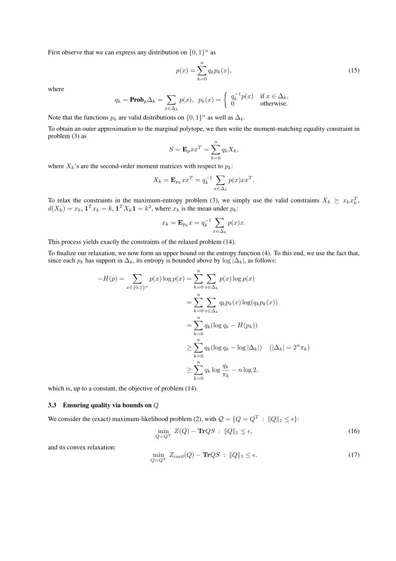
First observe that we can express any distribution on {0, 1}n as

p(x) =n∑

k=0

qkpk(x), (15)

where

qk = Probp∆k =∑

x∈∆k

p(x), pk(x) ={

q−1k p(x) if x ∈ ∆k,

0 otherwise.

Note that the functions pk are valid distributions on {0, 1}n as well as ∆k.

To obtain an outer approximation to the marginal polytope, we then write the moment-matching equality constraint inproblem (3) as

S = EpxxT =n∑

k=0

qkXk,

where Xk’s are the second-order moment matrices with respect to pk:

Xk = EpkxxT = q−1

k

∑

x∈∆k

p(x)xxT .

To relax the constraints in the maximum-entropy problem (3), we simply use the valid constraints Xk º xkxTk ,

d(Xk) = xk, 1T xk = k, 1T Xk1 = k2, where xk is the mean under pk:

xk = Epkx = q−1

k

∑

x∈∆k

p(x)x.

This process yields exactly the constraints of the relaxed problem (14).

To finalize our relaxation, we now form an upper bound on the entropy function (4). To this end, we use the fact that,since each pk has support in ∆k, its entropy is bounded above by log |∆k|, as follows:

−H(p) =∑

x∈{0,1}n

p(x) log p(x) =n∑

k=0

∑

x∈∆k

p(x) log p(x)

=n∑

k=0

∑

x∈∆k

qkpk(x) log(qkpk(x))

=n∑

k=0

qk(log qk −H(pk))

≥n∑

k=0

qk(log qk − log |∆k|) (|∆k| = 2nπk)

≥n∑

k=0

qk logqk

πk− n log 2,

which is, up to a constant, the objective of problem (14).

3.3 Ensuring quality via bounds on Q

We consider the (exact) maximum-likelihood problem (2), with Q = {Q = QT : ‖Q‖1 ≤ ε}:

minQ=QT

Z(Q)−TrQS : ‖Q‖1 ≤ ε, (16)

and its convex relaxation:min

Q=QTZcard(Q)−TrQS : ‖Q‖1 ≤ ε. (17)

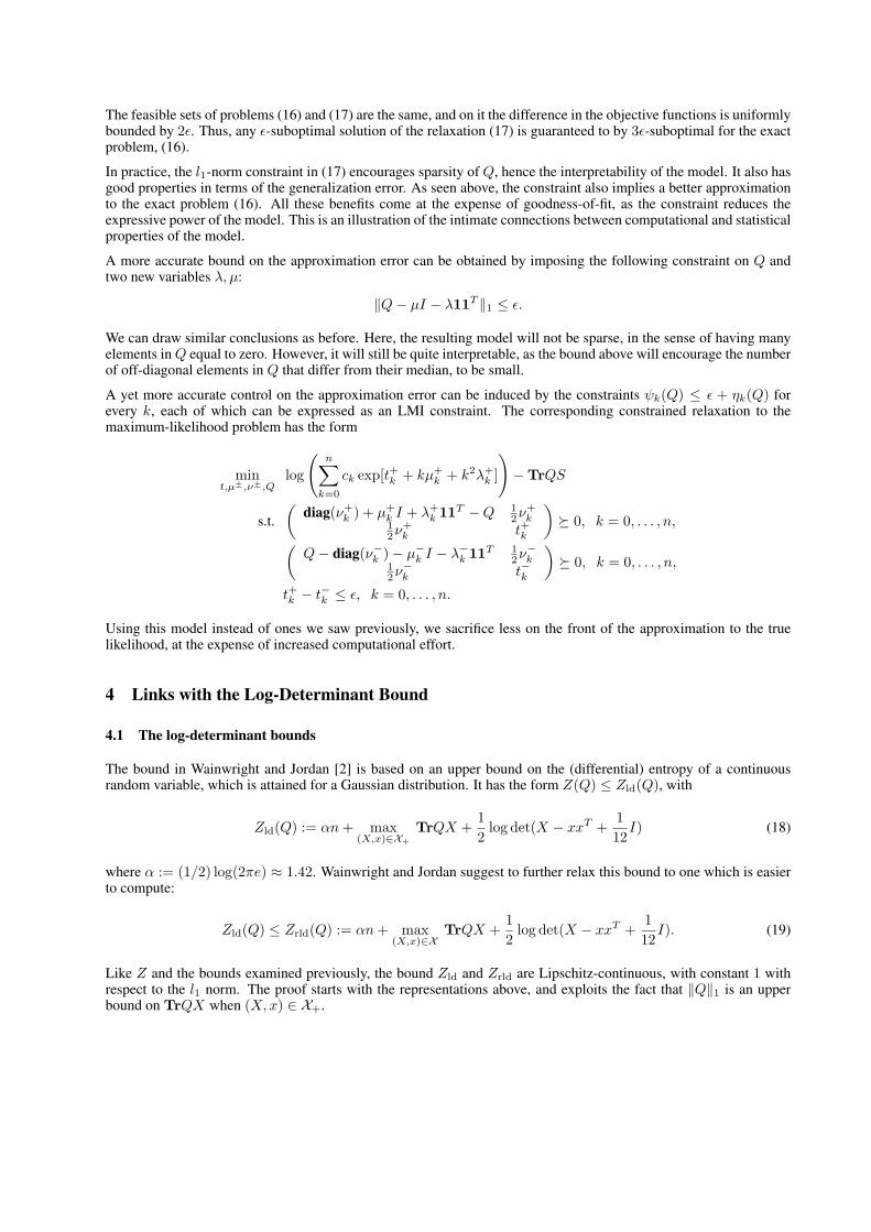
The feasible sets of problems (16) and (17) are the same, and on it the difference in the objective functions is uniformlybounded by 2ε. Thus, any ε-suboptimal solution of the relaxation (17) is guaranteed to by 3ε-suboptimal for the exactproblem, (16).

In practice, the l1-norm constraint in (17) encourages sparsity of Q, hence the interpretability of the model. It also hasgood properties in terms of the generalization error. As seen above, the constraint also implies a better approximationto the exact problem (16). All these benefits come at the expense of goodness-of-fit, as the constraint reduces theexpressive power of the model. This is an illustration of the intimate connections between computational and statisticalproperties of the model.

A more accurate bound on the approximation error can be obtained by imposing the following constraint on Q andtwo new variables λ, µ:

‖Q− µI − λ11T ‖1 ≤ ε.

We can draw similar conclusions as before. Here, the resulting model will not be sparse, in the sense of having manyelements in Q equal to zero. However, it will still be quite interpretable, as the bound above will encourage the numberof off-diagonal elements in Q that differ from their median, to be small.

A yet more accurate control on the approximation error can be induced by the constraints ψk(Q) ≤ ε + ηk(Q) forevery k, each of which can be expressed as an LMI constraint. The corresponding constrained relaxation to themaximum-likelihood problem has the form

mint,µ±,ν±,Q

log

(n∑

k=0

ck exp[t+k + kµ+k + k2λ+

k ]

)−TrQS

s.t.(

diag(ν+k ) + µ+

k I + λ+k 11T −Q 1

2ν+k

12ν+

k t+k

)º 0, k = 0, . . . , n,

(Q− diag(ν−k )− µ−k I − λ−k 11T 1

2ν−k12ν−k t−k

)º 0, k = 0, . . . , n,

t+k − t−k ≤ ε, k = 0, . . . , n.

Using this model instead of ones we saw previously, we sacrifice less on the front of the approximation to the truelikelihood, at the expense of increased computational effort.

4 Links with the Log-Determinant Bound

4.1 The log-determinant bounds

The bound in Wainwright and Jordan [2] is based on an upper bound on the (differential) entropy of a continuousrandom variable, which is attained for a Gaussian distribution. It has the form Z(Q) ≤ Zld(Q), with

Zld(Q) := αn + max(X,x)∈X+

TrQX +12

log det(X − xxT +112

I) (18)

where α := (1/2) log(2πe) ≈ 1.42. Wainwright and Jordan suggest to further relax this bound to one which is easierto compute:

Zld(Q) ≤ Zrld(Q) := αn + max(X,x)∈X

TrQX +12

log det(X − xxT +112

I). (19)

Like Z and the bounds examined previously, the bound Zld and Zrld are Lipschitz-continuous, with constant 1 withrespect to the l1 norm. The proof starts with the representations above, and exploits the fact that ‖Q‖1 is an upperbound on TrQX when (X,x) ∈ X+.

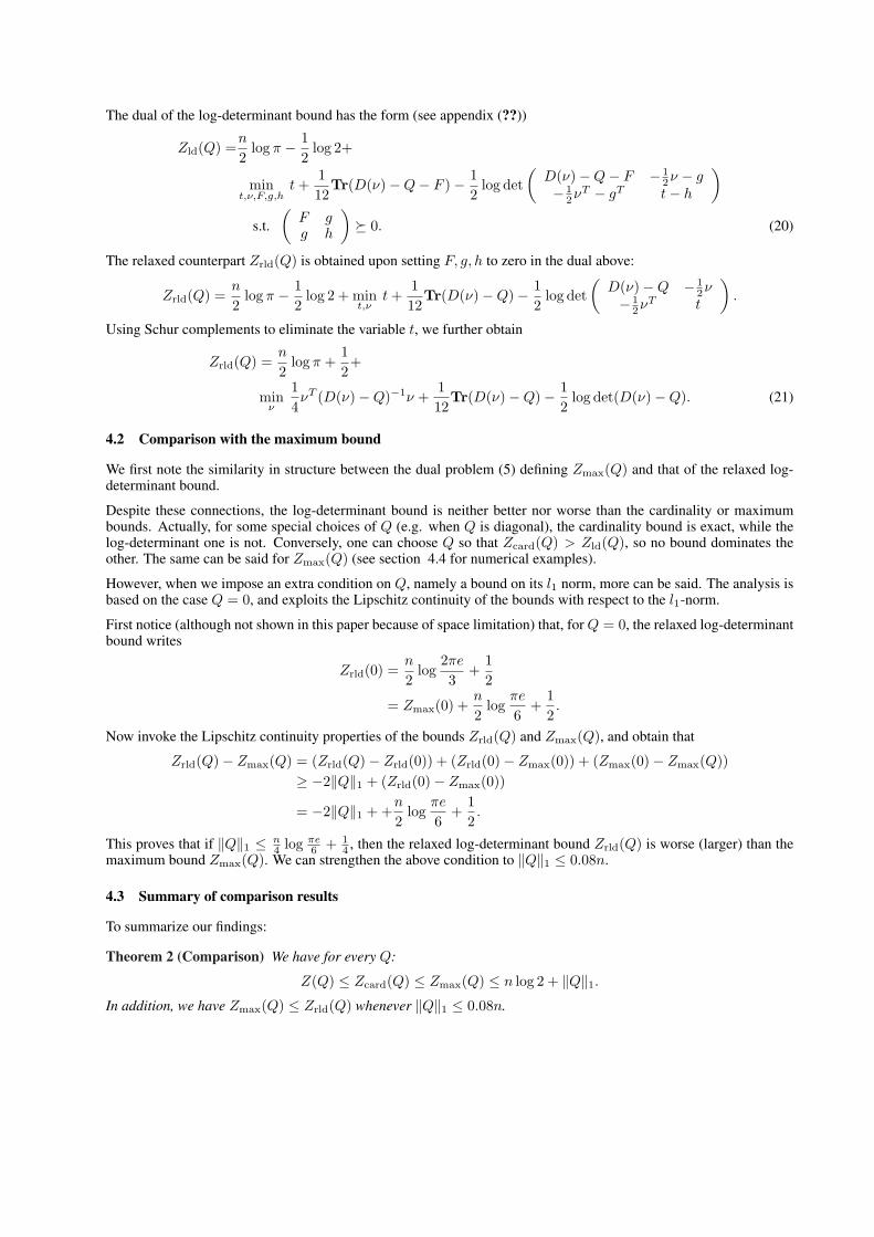
The dual of the log-determinant bound has the form (see appendix (??))

Zld(Q) =n

2log π − 1

2log 2+

mint,ν,F,g,h

t +112

Tr(D(ν)−Q− F )− 12

log det(

D(ν)−Q− F − 12ν − g

− 12νT − gT t− h

)

s.t.(

F gg h

)º 0. (20)

The relaxed counterpart Zrld(Q) is obtained upon setting F, g, h to zero in the dual above:

Zrld(Q) =n

2log π − 1

2log 2 + min

t,νt +

112

Tr(D(ν)−Q)− 12

log det(

D(ν)−Q − 12ν

− 12νT t

).

Using Schur complements to eliminate the variable t, we further obtain

Zrld(Q) =n

2log π +

12+

minν

14νT (D(ν)−Q)−1ν +

112

Tr(D(ν)−Q)− 12

log det(D(ν)−Q). (21)

4.2 Comparison with the maximum bound

We first note the similarity in structure between the dual problem (5) defining Zmax(Q) and that of the relaxed log-determinant bound.

Despite these connections, the log-determinant bound is neither better nor worse than the cardinality or maximumbounds. Actually, for some special choices of Q (e.g. when Q is diagonal), the cardinality bound is exact, while thelog-determinant one is not. Conversely, one can choose Q so that Zcard(Q) > Zld(Q), so no bound dominates theother. The same can be said for Zmax(Q) (see section 4.4 for numerical examples).

However, when we impose an extra condition on Q, namely a bound on its l1 norm, more can be said. The analysis isbased on the case Q = 0, and exploits the Lipschitz continuity of the bounds with respect to the l1-norm.

First notice (although not shown in this paper because of space limitation) that, for Q = 0, the relaxed log-determinantbound writes

Zrld(0) =n

2log

2πe

3+

12

= Zmax(0) +n

2log

πe

6+

12.

Now invoke the Lipschitz continuity properties of the bounds Zrld(Q) and Zmax(Q), and obtain that

Zrld(Q)− Zmax(Q) = (Zrld(Q)− Zrld(0)) + (Zrld(0)− Zmax(0)) + (Zmax(0)− Zmax(Q))≥ −2‖Q‖1 + (Zrld(0)− Zmax(0))

= −2‖Q‖1 + +n

2log

πe

6+

12.

This proves that if ‖Q‖1 ≤ n4 log πe

6 + 14 , then the relaxed log-determinant bound Zrld(Q) is worse (larger) than the

maximum bound Zmax(Q). We can strengthen the above condition to ‖Q‖1 ≤ 0.08n.

4.3 Summary of comparison results

To summarize our findings:

Theorem 2 (Comparison) We have for every Q:

Z(Q) ≤ Zcard(Q) ≤ Zmax(Q) ≤ n log 2 + ‖Q‖1.In addition, we have Zmax(Q) ≤ Zrld(Q) whenever ‖Q‖1 ≤ 0.08n.

4.4 A numerical experiment

We now illustrate our findings on the comparison between the log-determinant bounds and the cardinality and maxi-mum bounds. We set the size of our model to be n = 20, and for a range of values of a parameter ρ, generate N = 10random instances of Q with ‖Q‖1 = ρ. Figure ?? shows the average values of the bounds, as well as the associatederror bars. Clearly, the new bound outperforms the log-determinant bounds for a wide range of values of ρ. Ourpredicted threshold value of ‖Q‖1 for which the new bound becomes worse, namely ρ = 0.08n ≈ 1.6 is seen to bevery conservative, with respect to the observed threshold of ρ ≈ 30. On the other hand, we observe that for largevalues of ‖Q‖1, the log-determinant bounds do behave better. Across the range of ρ, we note that the log-determinantbound is indistinguishable from its relaxed counterpart.

5 Conclusion and Remarks

We have introduced a new upper bound (the cardinality bound) for the log-partition function corresponding to second-order Ising models for binary distribution. We have shown that such a bound can be computed via convex optimization,and, when compared to the log-determinant bound introduced by Wainwright and Jordan (2006), the cardinality boundperforms better when the l1-norm of the model parameter vector is small enough.Although not shown in the paper, the cardinality bound becomes exact in the case of standard Ising model, while themaximum bound (for example) is not exact for such model.As was shown in section 2, the cardinality bound was computed by defining a partition of {0, 1}. This idea can begeneralized to form a class of bounds which we call partition bounds. It turns out that partitions bound are closelylinked to the more general class bounds that are based on worst-case probability analysis.We acknowledge the importance of applying our bound to real-word data. We hope to include such results in subse-quent versions of this paper.

References

[1] P. Ravikumar and J. Lafferty. Variational Chernoff bounds for graphical models. In Proc. Advances in NeuralInformation Processing Systems (NIPS), December 2007.

[2] Martin J. Wainwright and Michael I. Jordan. Log-determinant relaxation for approximate inference in discreteMarkov random fields. IEEE Trans. Signal Processing, 2006.