beta-Ensembles for Toric Orbifold Partition Function

271

Progress of Theoretical Physics, Vol. 127, No. 2, February 2012

β-Ensembles for Toric Orbifold Partition Function

Taro Kimura1,2,∗)

1Department of Basic Science, University of Tokyo, Tokyo 153-8902, Japan2Mathematical Physics Lab., RIKEN Nishina Center, Wako 351-0198, Japan

(Received September 9, 2011; Revised December 9, 2011)

We investigate combinatorics of the instanton partition function for the generic fourdimensional toric orbifolds. It is shown that the orbifold projection can be implementedby taking the inhomogeneous root of unity limit of the q-deformed partition function. Theasymptotics of the combinatorial partition function yields the multi-matrix model for ageneric β.

Subject Index: 135, 183

§1. Introduction

The instanton counting is extensively applied to various non-perturbative as-pects of the four dimensional gauge theory. In particular Nekrasov partition func-tion1),2) plays an essential role not only in the four dimensional Seiberg-Wittentheory,3),4) but also the two dimensional conformal field theory. The remarkableconnection between the four and two dimensional theories through the instantonpartition function is called AGT relation,5) and generalized to various situations, forexample, the higher rank theory,6),7) the asymptotic free theory8)–10) and also theALE space,11)–15) etc.

The ALE space is given by resolving the singularity of the orbifold C2/Γ .16)–18)

The instanton construction,19),20) the instanton counting21) and the wall-crossing22),23) are considered in this case as well as the Euclidean space R

4 � C2.

Furthermore the inhomogeneous orbifold theory is discussed in terms of the AGTrelation:24) it is shown that the instanton counting on the inhomogeneous orbifoldC × C/Zr is utilized to describe the theory in the presence of a generic surface op-erator. Not only the four dimensional theory, but also the two dimensional theorywith vortices on orbifolds has been recently investigated.25)

In this paper we develop the previous result,26) and consider a systematic methodto deal with the combinatorial representation of the partition function for the genericfour dimensional toric orbifolds C

2/Γr,s, whose boundary is the generic lens spaceL(r, s). It includes the type Ar−1 ALE space as C

2/Γr,r−1 = C2/Zr. So far N = 4

theories on such a space, and also Chern-Simons theory on the lens space L(r, s)have been investigated.27)–30) Recently further research is done with respect to theindex, and its relation to the three and two dimensional theories.31)

We can obtain the orbifold partition function by performing the orbifold projec-tion for the standard one. However it is apparently written in a complicated form,

∗) E-mail: [email protected]

272 T. Kimura

we will show a much simpler method to assign the orbifold projection. To imple-ment that we first lift it up to the q-deformed theory, and then take the root of unitylimit of it, as well as the standard orbifold C

2/Zr discussed in Ref. 26). The similarmethod is also applied to the spin Calogero-Sutherland model32) (see also Ref. 33)).

We also discuss the β-ensemble matrix model for the toric orbifold theories. Wesuccessfully obtain the multi-matrix model with a generic β by extracting the asymp-totics of the combinatorial partition function.35)–37) The Ω-background parameteris related to this parameter as β = −ε2/ε1, so that it is important to discuss thegeneric β-ensemble in order to consider the application to the AGT relation. Whenwe estimate the asymptotic behavior of the combinatorial part corresponding to thematrix measure, we need the root of unity limit of the q-deformed Vandermondedeterminant, which is the weight function for the Macdonald polynomial.38) Thissuggests that we can obtain a new kind of polynomials induced from the Macdonaldpolynomial by taking this limit.

This paper is organized as follows. In §2 we consider the ADHM constructionfor the toric orbifolds C

2/Γr,s, and then obtain the combinatorial expression for thepartition function. We will show that the root of unity limit of the q-deformedpartition function is essential for the orbifold projection, and it is useful to introducethe basis of the fractional exclusive statistics. Section 3 is devoted to derivation ofthe matrix models. We obtain the β-ensemble multi-matrix model by taking theasymptotic limit of the combinatorial partition function. In §4 we summarize theresults with some discussions.

§2. Instanton counting on toric orbifolds

Let us start with the generic four dimensional toric space. It is given by thequotient C

2/Γr,s where Γr,s is a Zr action labeled by the two coprime integers (r, s)with 0 < s < r as

Γr,s : (z1, z2) −→ (ωrz1, ωsrz2), (2.1)

where ωr = exp(2πi/r) is the primitive r-th root of unity. This space goes to thelens space L(r, s) at infinity.

The orbifold action (2.1) generates a singularity at the origin of C2. We can ob-

tain the smooth manifold by resolving the singularity, which is called the Hirzebruch-Jung space.39) After blowing up the singularity there are � two-spheres characterizedby the generalized Cartan matrix

C =

⎛⎜⎜⎜⎜⎜⎝−e1 1 0 · · · 01 −e2 1 · · · 00 1 −e3 · · · 0...

......

. . ....

0 0 0 · · · −e�

⎞⎟⎟⎟⎟⎟⎠ , (2.2)

where the self-intersection numbers ei, i = 2, · · · , � are obtained by expanding the

β-Ensembles for Toric Orbifold Partition Function 273

rational number r/s in a continued fraction form

r

s= e1 − 1

e2 −1

e3 −1

. . . e�−1 −1e�

(2.3)

and e1 is the smallest integer greater than r/s. In the case of the ALE space, namelys = r − 1, we have ei = 2 and � = r − 1. Therefore the matrix (2.2) coincides withthe Cartan matrix for the type-Ar−1 Lie algebra.

We then consider the standard ADHM construction for R4 � C

2 to study instan-ton counting before orbifolding. The ADHM equations for k-instanton configurationfor SU (n) theory are given by

EC := [B1, B2] + IJ = 0, (2.4)

ER := [B1, B†1] + [B2, B

†2] + II† − J†J = 0, (2.5)

where the ADHM data (B1, B2, I, J) are interpreted as elements of homomorphisms,

B1, B2 ∈ Hom (V, V ) , I ∈ Hom (W, V ) , J ∈ Hom (V, W ) . (2.6)

The rank of the gauge group and the instanton number are encoded in dimensionsof the vector spaces, dim V = n and dim W = k, respectively. Actually, when weconsider SU (n) theory, we had better deal with U (n) group, and then implementthe condition for the Coulomb moduli

∑nl=1 al = 0. Note that this procedure is

not enough for some cases: we have to factor out the U (1) contribution when weconsider the AGT relation.5)

There is U (k) gauge symmetry for these ADHM data

(B1, B2, I, J) −→ (gB1g

−1, gB2g−1, gI, Jg−1

), g ∈ U (k), (2.7)

and thus the instanton moduli space is given by

Mn,k = {(B1, B2, I, J)|EC = 0, ER = 0} /U (k). (2.8)

The resolution of singularity of this ADHM moduli space is given by the followingquotient,40)

M̃n,k = {(B1, B2, I, J)|EC = 0, stability cond.} //GL(k, C). (2.9)

The stability condition is interpreted as the irreducibility for the moduli space.We then consider the action of isometries on C

2 for the ADHM data

(B1, B2, I, J) −→ (T1B1, T2B2, IT−1

a , T1T2TaJ), (2.10)

where Ta = diag(eia1 , · · · , eian) ∈ U (1)n, Tα = eiεα ∈ U (1)2. They are the torusactions coming from the symmetry of U (n) and SO(4), respectively. We have to

274 T. Kimura

consider the fixed point of these isometries up to gauge transformation g ∈ U (k) toperform the localization formula. Thus the orbifold action, corresponding to (2.1),on the ADHM data is

Γr,s : (B1, B2, I, J) −→ (ωrB1, ωsrB2, I, ω1+s

r J). (2.11)

Due to the orbifold action we have to introduce decomposed vector spaces withrespect to the irreducible representations of Zr,

W =r⊕

v=1

Wv, V =r⊕

v=1

Vv. (2.12)

Here we assign the orbifold action for the gauge group element as eial → ωplr eial . It

is just a holonomy, which characterizes the boundary condition of the gauge field.Thus the ADHM data surviving under the orbifold action can be written as

B1,v ∈ Hom(Vv, Vv+1), B2,v ∈ Hom(Vv, Vv+s),Iv ∈ Hom(Wv, Vv), Jv ∈ Hom(Vv, Wv+1+s), (2.13)

and thus we have

EC −→ B1,v+sB2,v − B2,v+1B1,v + Iv+1+sJv, (2.14)

ER −→ B1,v−1B†1,v−1 − B†

1,vB1,v + B2,v−sB†2,v−s − B†

2,vB2,v + IvI†v − JvJ

†v . (2.15)

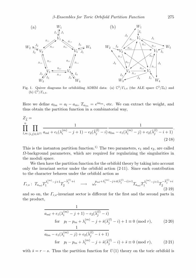
They are periodic modulo r as Wr+1 = W1 and so on. Figure 1 shows quiver diagramsfor orbifolding ADHM data. These conditions are much complicated, and thus thewhole structure of the instanton moduli space is not yet clear. Actually (2.14) and(2.15) take non-zero value after resolving the singularity. It can concern possibilityof the localization method. Its availability is investigated for the case of the ALEspace21) and more generic theories,41),42) but we have to consider this problem moreexplicitly. Basically we still have the isometry U (1)2 corresponding to the spatialrotation even for the orbifolds. This might ensure that we can apply the localizationformula to these cases.

We then derive the combinatorial representation of the partition function. Sincethe characters of the vector spaces are given by

V =n∑

l=1

∑(i,j)∈λ(l)

TalT 1−i

1 T 1−j2 , W =

n∑l=1

Tal, (2.16)

the character of the tangent space at the fixed point under the isometries, which islabeled by n-tuple partition λ, turns out to be

χ�λ= −V ∗V (1 − T1)(1 − T2) + W ∗V + V ∗WT1T2

=n∑

l,m

∑(i,j)∈λ(l)

(Taml

Tλ(m)i −j+1

1 T−λ̌

(l)j +i

2 + TalmT−λ

(m)i +j

1 Tλ̌(l)j −i+1

2

). (2.17)


Fig. 1. Quiver diagrams for orbifolding ADHM data: (a) C2/Γ5,4 (the ALE space C

2/Z5) and

(b) C2/Γ5,3.

Here we define alm = al − am, Talm= eialm , etc. We can extract the weight, and

thus obtain the partition function in a combinatorial way,

Z�λ=

n∏l,m

∏(i,j)∈λ(l)

1

aml + ε1(λ(m)i − j + 1) − ε2(λ̌

(l)j − i)

1

alm − ε1(λ(m)i − j) + ε2(λ̌

(l)j − i + 1)

.

(2.18)

This is the instanton partition function.1) The two parameters, ε1 and ε2, are calledΩ-background parameters, which are required for regularizing the singularities inthe moduli space.

We then have the partition function for the orbifold theory by taking into accountonly the invariant sector under the orbifold action (2.11). Since each contributionto the character behaves under the orbifold action as

Γr,s : TamlT

λ(m)i −j+1

1 T−λ̌

(l)j +i

2 −→ ωpml+λ

(m)i −j+s̄(λ̌

(l)j −i)+1

r TamlT

λ(m)i −j+1

1 T−λ̌

(l)j +i

2

(2.19)and so on, the Γr,s-invariant sector is different for the first and the second parts inthe product,

1

aml + ε1(λ(m)i − j + 1) − ε2(λ̌

(l)j − i)

for pl − pm + λ(m)i − j + s̄(λ̌(l)

j − i) + 1 ≡ 0 (mod r), (2.20)1

alm − ε1(λ(m)i − j) + ε2(λ̌

(l)j − i + 1)

for pl − pm + λ(m)i − j + s̄(λ̌(l)

j − i) + s̄ ≡ 0 (mod r), (2.21)

with s̄ = r − s. Thus the partition function for U (1) theory on the toric orbifold is

276 T. Kimura

given by

Zλ;Γr,s =∏

Γ̌ -inv.⊂λ

1λi − j + β(λ̌j − i) + 1

∏Γ̂ -inv.⊂λ

1λi − j + β(λ̌j − i) + β

. (2.22)

We introduce another parameter defined as β = −ε2/ε1. Here Γ̌ - and Γ̂ -invariantsectors stand for the conditions shown in (2.20) and (2.21), respectively. It can beeasily extended to SU (n) gauge theory.

These conditions to extract the Γr,s-invariant sectors are apparently complicated,but there is a simple way to implement the orbifold projection.26),32) To implementthe orbifold projection, let us start with the standard partition function before orb-ifolding, and then lift it to the q-deformed partition function, which is interpretedas the five dimensional function,

Zqλ =

∏(i,j)∈λ

1

1 − qλi−j+1tλ̌j−i

1

1 − q−λi+jt−λ̌j+i−1. (2.23)

These q and t are related to the Ω-background parameters as q = eε1 , t = e−ε2 = qβ.Of course we obtain the original four dimensional function by taking the usual q → 1limit. On the other hand, by taking the root of unity limit of the q-deformed function,the orbifolded partition function (2.22) is automatically obtained up to constants.In this case we assign the following parametrization,

q −→ ωrq, t −→ ω−sr qβ = ωs̄

rqβ (2.24)

and then take the limit q → 1. To regularize the singular behavior at q → 1, we nowtake into account the adjoint matter contribution whose mass parameter is given bym. Thus the weight function yields, for example,

1 − ωλi−j+s̄(λ̌j−i)+1r qλi−j+1+mtλ̌j−i

1 − ωλi−j+s̄(λ̌j−i)+1r qλi−j+1tλ̌j−i

−→{

λi−j+β(λ̌j−i)+1+m

λi−j+β(λ̌j−i)+1if λi − j + s̄(λ̌j − i) + 1 ≡ 0 (mod r)

1 if λi − j + s̄(λ̌j − i) + 1 �≡ 0 (mod r). (2.25)

If we want to extract only the contribution of the vector multiplet, we have to takethe decoupling limit m → ∞.

The q-partition function for SU (n) theory can be written with the cutoff para-meter N (l) for the number of entries of the partitions as follows:

Zq�λ

=∏

(l,i) �=(m,j)

(Qlmqλ(l)i −λ

(m)j tj−i; q)∞

(Qlmqλ(l)i −λ

(m)j tj−i+1; q)∞

n∏l,m

N(l)∏i=1

(Qlmqλ(l)i tN

(m)−i+1; q)∞(Qmlq

−λ(l)i t−N(m)+i; q)∞

. (2.26)

Here (x; q)n =∏n−1

m=0(1−xqm) is the q-Pochhammer symbol, and the Coulomb mod-uli is denoted as Qlm = ealm = qblm . Note that this q-partition function includes theinfinite product, so that we have to take care of its radius of convergence. Therefore


Fig. 2. Decomposition of the partition λ = (5, 2, 2, 1) for C2/Γ3,1. A rectangular box is required

for obtaining the correspondence between the partition and the particle description with the

repulsion parameter s̄ = r − s.

we first consider the parametrization (2.24), and then take the limit q → 1. Thisorbifold projecting procedure is quite useful, for example, to investigate asymptoticbehavior of the orbifold partition function because it can be simply given by studyingasymptotics of the q-partition function in a usual way, and taking its root of unitylimit at last.

We now comment on the relation to the explicit expressions for OP1(−r), etc.which is shown in Refs. 27) and 42). They are written down in terms of the localcoordinates of the resolved space. For example, in the case of OP1(−r), they aregiven by (z(1)

1 , z(1)2 ) = (zr

1, z−11 z2) and (z(2)

1 , z(2)2 ) = (z1z

−12 , zr

2), which are invariantunder (z1, z2) → (ωrz1, ωrz2). Thus we have the instanton partition function, whichis manifestly invariant under the orbifold action. This manipulation gives rise toredefinition of the partitions: if we consider U (1) theory for simplicity, we haveλi → λ

(1)I , λ

(2)I , which satisfy λi = rλ

(1)I +I with i = I or λi = λ

(2)I with i = λ

(2)I +rI.

Here the superscript labels the local patch of the resolved space. The expressionsfor OP1(−r) can be obtained by these redefined variables. Anyway this connectionis still complicated, thus it should be investigated in detail for further study.

To treat the orbifold partition function more conveniently, we then try to de-compose the partitions. In this case we introduce a slightly different way of decom-position,26),43)

r(λ(l,v)i + N (l,v) − i + p(l,v)) + v ≡ λ

(l)j + s̄(N (l) − j) + pl, j = c

(l,v)i , (2.27)

where c(l,v)i stands for the mapping from the index of the divided nr-partition to that

of the original n-partition. Figure 2 shows an example for the case with the orbifoldC

2/Γ3,1, namely s̄ = 2.This decomposition is based on the particle description obeying the fractional

exclusive statistics,44) which is deeply related to Calogero-Sutherland model (see,for example, Ref. 33)). The parameter s̄ stands for the strength of the repulsionbetween particles, and this generalized statistics goes back to the usual fermionicone in the case of the ALE space, s̄ = 1. It is useful to introduce a rectangular boxto obtain the correspondence between the partition and the particle description dueto the repulsion parameter s̄.

278 T. Kimura

Introducing another set of variables defined as

�(l,v)i ≡ r(λ(l,v)

i + N (l,v) − i + p(l,v)) + bl − pl + v, (2.28)

we finally obtain r-tuple partition by blending nr-tuple one,

�(v)

i=1,··· ,Pnl=1 N(l,v) =

(�(n,v)1 , · · · , �

(n,v)

N(n,v), · · · , �(1,v)1 , · · · , �

(1,v)

N(1,v)

). (2.29)

We now assume N (l) = N and N (l,v) = N for simplicity. Thus the partition functionis rewritten in terms of r-tuple partition,

Zq�λ

=∏

(v,i) �=(w,j)

(ωv−wr q�

(v)i −�

(w)j +(β−s̄)(c

(w)j −c

(v)i ); ωrq)∞

(ωv−w+s̄r q�

(v)i −�

(w)j +(β−s̄)(c

(w)j −c

(v)i )+β; ωrq)∞

×n∏

l=1

r−1∏v=0

nN∏i=1

(ωr−pl+s̄q�(v)i −bl+(β−s̄)(N−c

(v)i )+β; ωrq)∞

(ω−r+plq−(�(v)i −bl+(β−s̄)(N−c

(v)i )); ωrq)∞

. (2.30)

Let c(v)i stand for the mapping of the index from r-tuple to nr-tuple partition as

before.

§3. Matrix model description

We then derive matrix model description by taking asymptotic limit of the com-binatorial representation of the partition function (2.30). Such an integral represen-tation would be useful to extract the gauge theory consequences by performing thelarge N limit analysis: the Seiberg-Witten curve is obtained from the spectral curveof the matrix model.26),34),35)

We now consider the following function to study the asymptotics of the partitionfunction,

fq,t(x) =(x; q)∞(tx; q)∞

. (3.1)

The asymptotics of this function is almost given by the limit of |q| → 1 because,when x = ey, we have

fq,t(x) =∞∏

n=0

1 − ey+nε1

1 − ey+(n+β)ε1. (3.2)

Therefore the condition y � ε1 corresponds to the limit q → 1. This function isinvestigated in detail in Appendix A.

Thus we now apply the result for the double root of unity limit (A.13) to thecombinatorially represented partition function. Introducing the following variables

x(v)i =

�(v)i

ε1, (3.3)

and taking the limit ε1 → 0, we then obtain the matrix model representation whichcaptures the asymptotics of the combinatorial partition function. For the orbifold


C2/Γr,s, we have the r-matrix model,

Z =∫

D X e− 1

ε1

Pr−1v=0

PNi=1 V (x

(v)i )

, (3.4)

D X =r−1∏v=0

N∏i=1

dx(v)i

2πΔ2(x). (3.5)

Note that we have to replace the summation over the partition with the integral ofthe continuous variables. This is done by inserting an auxiliary function, which hasa simple pole at all integer values of the argument.35)–37) This affects on the matrixintegral as just a linear shift of the matrix potential in the large N limit, which canbe absorbed by the counting parameter.

Let us now discuss the matrix measure and the potential function. Accordingto (A.13), asymptotics of the first part in (2.30), which will go to the measure partof the matrix model, yields∏

(v,i) �=(w,j)

fq,t

(ωv−w

r q�(v)i −�

(w)j +(β−s̄)(c

(w)j −c

(v)i )

)

�∏

(v,i) �=(w,j)

[(1 − er(x

(v)i −x

(w)j )

)(β−s̄)/r s̄−1∏k=0

(1 − ωv−w+k

r ex(v)i −x

(w)j

)]. (3.6)

This coincides with the following matrix measure, up to the overall factor,

Δ2(x) =r−1∏v=0

N∏i<j

[(2 sinh

r

2

(x

(v)i − x

(v)j

))2(β−s̄)/rs̄−1∏k=0

(2 sinh

12

(x

(v)i − x

(v)j +

2πi

rk

))2s̄]

×r−1∏v<w

N∏i,j

[(2 sinh

r

2

(x

(v)i − x

(w)j

))2(β−s̄)/r

×s̄−1∏k=0

(2 sinh

12

(x

(v)i − x

(w)j +

2πi

r(v − w + k)

))2]. (3.7)

We redefine the matrix size as nN → N for convenience. We remark that β cantake a generic value, thus (3.7) is interpreted as the measure part of the β-ensemblematrix model for the generic toric orbifold.

The corresponding four dimensional limit is given by

Δ2(x) →r−1∏v=0

N∏i<j

(x

(v)i − x

(v)j

)2(β−s̄)/r+2s̄r−1∏v<w

N∏i,j

(x

(v)i − x

(w)j

)2(β−s̄)/r+2Ns̄(v−w),(3.8)

where we define Ns̄(x) = #{k|x + k ≡ 0 (mod r), k = 0, · · · , s̄ − 1}.We can easily obtain important examples from this generic result. For the case

280 T. Kimura

of s̄ = 1, corresponding to the orbifold C2/Zr, we have

Δ2(x) =r−1∏v=0

N∏i<j

[(2 sinh

r

2

(x

(v)i − x

(v)j

))2(β−1)/r(

2 sinh12

(x

(v)i − x

(v)j

))2]

×r−1∏v<w

N∏i,j

[(2 sinh

r

2

(x

(v)i − x

(w)j

))2(β−1)/r

×(

2 sinh12

(x

(v)i − x

(w)j +

2πi

r(v − w)

))2]. (3.9)

This is consistent with the previous result.26) In this time this formula is availableeven for generic β while only the specific case β = rγ+1 ≡ 1 (mod r), γ = 0, 1, 2, · · · ,is investigated in the previous paper. This generalization is quite important because,in terms of AGT relation, the parameter β plays a crucial role in both of the fourdimensional and two dimensional theories.

The second is the case s̄ = r, corresponding to the orbifold C × C/Zr,

Δ2(x) =∏

(v,i) �=(w,j)

(2 sinh

r

2

(x

(v)i − x

(w)j

))2β/r

→∏

(v,i) �=(w,j)

(x

(v)i − x

(w)j

)2β/r. (3.10)

This case is also important to study the instanton counting in presence of the genericsurface operators as discussed in Ref. 24).

We then consider the potential part for the matrix model. It is useful to discussthe quantum dilogarithm function45) for deriving the matrix potential,

g(z; q) =∞∏

p=1

(1 − 1

zqp

). (3.11)

In particular, when we parametrize q = eε1 , the asymptotic behavior at the root ofunity26) is given by

log g(z; ωrq) =1ε1

[1r2

Li2

(1zr

)+ O(ε1)

], (3.12)

where Li2(x) =∑∞

p=1 zp/p2 is the dilogarithm function. Thus the second part in(2.30) leads to the matrix potential,

n∏l=1

r−1∏v=0

nN∏i=1

(ωr−pl+s̄q�(v)i −bl+(β−s̄)(N−c

(v)i )+β; ωrq)∞

(ω−r+plq−(�(v)i −bl+(β−s̄)(N−c

(v)i )); ωrq)∞

≡ expr−1∑v=0

nN∑i=1

− 1ε1

V (x(v)i ),

(3.13)

V (x) = − 1r2

n∑l=1

[Li2(er(x−al)) − Li2(e−r(x−al))

]+ O(ε1). (3.14)


This potential function is completely the same as the previous result.26) It dependson only r, but s̄ nor β. The corresponding four dimensional limit is given by

V (x) −→ 2r

n∑l=1

[(x − al) log(x − al) − (x − al)] . (3.15)

In this paper we concentrate on the case without the matter fields, but it is expectedthat we can obtain the same matrix potential to the homogeneous orbifolds C

2/Zr

as well as the vector multiplet.

§4. Summary and discussion

In this paper we have extended the previous results26) to the toric orbifoldsC

/Γr,s with a generic deformation parameter β. The instanton counting on such aninhomogeneous orbifold would play an essential role on the AGT relation in presenceof the surface operator.24) Furthermore, since this parameter β is directly relatedto the Ω-background parameter as β = −ε2/ε1, it is important to assign a genericvalue for the application to the AGT relation.

We have considered the ADHM construction for the toric orbifolds C2/Γr,s, and

derived the instanton partition function for such a space. We have shown that theroot of unity limit is useful to implement the orbifold projection. It has been alsoshown that the partition function is well described by the particles obeying thefractional exclusive statistics for the generic case.

On the basis of such a combinatorial description, we have obtained the corre-sponding β-ensemble multi-matrix models by considering its asymptotic behavior.The matrix measure is directly related to the root of unity limit of the q-deformedVandermonde determinant, and reflecting the structure of the orbifolds C

2/Γr,s. Onthe other hand, the matrix potential depends on only r, but s.

We concentrate on obtaining the matrix model description in this paper, but wedo not deal with the matrix model itself in detail. Actually the matrix model, whichwe have derived, has an apparently complicated expression. However, this matrixmodel is obtained by the non-standard reduction of the q-deformed theory, whichshould be integrable because it can be represented in terms of the q-free boson fields.Thus it is expected that there is an integrable structure even for our matrix model.In the large N limit we could perform the standard treatment of the matrix model aswell as the generic lens space matrix model,29) and obtain the corresponding Seiberg-Witten curve as the spectral curve. Furthermore, the relation between the modeldiscussed in this paper and another kind of matrix model, i.e. Dijkgraaf and Vafa’smodel,34) is worth studying in detail, because the latter plays an essential role in theAGT relation. It is one of the possibilities of further study beyond this work.

It is also interesting to discuss the corresponding two dimensional conformalfield theory to the generic toric orbifold theory. Since the inhomogeneous orbifoldtheory is utilized to study the instanton partition function in presence of a surfaceoperator,24) it is expected to obtain a similar structure for the generic toric orbifoldtheory, corresponding to the para-Liouville/Toda theory.12) It would provide a novel

282 T. Kimura

perspective to explore an exotic conformal field theory.

Acknowledgements

The author would like to thank T. Nishioka and Y. Tachikawa for valuablecomments. The author is supported by Grant-in-Aid for JSPS Fellows.

Appendix AReduction of the q-Vandermonde Determinant

The function (3.1) is directly related to the weight function of the Macdonaldpolynomial,38) namely the q-deformed Vandermonde determinant,

Δ2q,t(x) =

∏i�=j

(xi/xj ; q)∞(txi/xj ; q)∞

=∏i�=j

fq,t(xi/xj). (A.1)

According to the q-binomial theorem we have

f−1q,t (x) =

∞∑n=0

(t; q)n

(q; q)nxn. (A.2)

In this appendix we investigate several kinds of reduction of the q-deformedVandermonde determinant.

The first example is given by the following parametrization,

t = qβ, q −→ 1. (A.3)

Because the coefficient becomes

(t; q)n

(q; q)n−→ (−1)n

( −βn

), (A.4)

we have

f−1q,t (x) −→

∞∑n=0

(−x)n

( −βn

)= (1 − x)−β. (A.5)

This corresponds to the Jack limit of the Macdonald polynomial since the q-Vandermonde is reduced to

Δ2q,t(x) −→

∏i�=j

(1 − xi

xj

)β

∼∏i<j

(xi − xj)2β. (A.6)

The same kind of reduction is found for the q-Virasoro algebra,46) which leads to theusual Virasoro algebra with the central charge c = 1 − 6(β − 1)2/β.

The next is the single root of unity limit, which is used to study the instantoncounting on the orbifold C

2/Zr,26) and corresponds to the parametrization proposedin 32),

q −→ ωrq, t −→ ωrqβ, q −→ 1. (A.7)


The expansion coefficient in (A.2) is given by

(t; q)n

(q; q)n=

n∏m=1

1 − ωmr tqm−1

1 − ωmr qm

−→[n/r]∏m=1

β + rm − 1rm

= (−1)[n/k]

(−(

β−1r + 1

)[n/r]

). (A.8)

Here [x] denotes the largest integer not greater than x. Therefore we have

f−1q,t (x) −→

∞∑n=0

(−xr)n

(−(

β−1r + 1

)n

)(1 + x + · · · + xr−1

)= (1 − x)−1 (1 − xr)−(β−1)/r . (A.9)

As a result, the q-Vandermonde is reduced as

Δ2q,t(x) −→

∏i�=j

(1 − xi

xj

)(1 − xr

i

xrj

)(β−1)/r

∼∏i<j

(xi − xj)2(xr

i − xrj

)2(β−1)/r.

(A.10)This is consistent with the previous result.26),32) Note that this reduction is availablefor generic positive β while only the specific case β = rγ + 1 ≡ 1 (mod r) has beeninvestigated so far.

The last is the double root of unity limit. We now consider the following para-metrization,

q −→ ωrq, t −→ ωs̄rq

β, q −→ 1. (A.11)

The coefficient in (A.2) becomes

(t; q)n

(q; q)n−→

s̄−1∏m=1

1 − ωn+mr

1 − ωmr

[n/r]∏m=1

(β − s̄)/r + m

m

= (−1)[n/r]

(−(

β−s̄r + 1

)[n/r]

)s̄−1∏m=1

1 − ωn+mr

1 − ωmr

. (A.12)

Note that this coefficient vanishes as (t; q)n/(q; q)n = 0 when n ≡ r− s̄+1, · · · , r−1(mod r). Thus we have a similar result,

f−1q,t (x) −→ (1 − xr)−(β−s̄)/r

s̄−1∏k=0

(1 − ωkr x)−1. (A.13)

This corresponds to the following reduction of the q-Vandermonde,

Δ2q,t(x) −→

∏i�=j

(1 − xr

i

xrj

)(β−s̄)/r s̄−1∏k=0

(1 − ωk

r

xi

xj

). (A.14)

284 T. Kimura

Especially, when s̄ = r, corresponding to the orbifold C×C/Zr, which is well inves-tigated in Ref. 24), it becomes

Δ2q,t(x) −→

∏i�=j

(1 − xr

i

xrj

)β/r

∼∏i<j

(xri − xr

j)2β/r. (A.15)

References

1) N. Nekrasov, Adv. Theor. Math. Phys. 7 (2004), 831, hep-th/0206161.2) N. Nekrasov and A. Okounkov, hep-th/0306238.3) N. Seiberg and E. Witten, Nucl. Phys. B 426 (1994), 19, hep-th/9407087.4) N. Seiberg and E. Witten, Nucl. Phys. B 431 (1994), 484, hep-th/9408099.5) L. F. Alday, D. Gaiotto and Y. Tachikawa, Lett. Math. Phys. 91 (2010), 167,

arXiv:0906.3219.6) N. Wyllard, J. High Energy Phys. 11 (2009), 002, arXiv:0907.2189.7) A. Mironov and A. Morozov, Nucl. Phys. B 825 (2010), 1, arXiv:0908.2569.8) D. Gaiotto, arXiv:0908.0307.9) A. Marshakov, A. Mironov and A. Morozov, Phys. Lett. B 682 (2009), 125,

arXiv:0909.2052.10) M. Taki, J. High Energy Phys. 05 (2011), 038, arXiv:0912.4789.11) V. Belavin and B. Feigin, J. High Energy Phys. 07 (2011), 079, arXiv:1105.5800.12) T. Nishioka and Y. Tachikawa, Phys. Rev. D 84 (2011), 046009, arXiv:1106.1172.13) G. Bonelli, K. Maruyoshi and A. Tanzini, J. High Energy Phys. 08 (2011), 056,

arXiv:1106.2505.14) A. Belavin, V. Belavin and M. Bershtein, J. High Energy Phys. 09 (2011), 117,

arXiv:1106.4001.15) G. Bonelli, K. Maruyoshi and A. Tanzini, arXiv:1107.4609.16) T. Eguchi and A. J. Hanson, Phys. Lett. B 74 (1978), 249.17) G. Gibbons and S. Hawking, Phys. Lett. B 78 (1978), 430.18) P. B. Kronheimer, J. Diff. Geom. 29 (1989), 665.19) H. Nakajima, Invent. Math. 102 (1990), 267.20) P. B. Kronheimer and H. Nakajima, Math. Ann. 288 (1990), 263.21) F. Fucito, J. F. Morales and R. Poghossian, Nucl. Phys. B 703 (2004), 518, hep-

th/0406243.22) T. Nishinaka and S. Yamaguchi, arXiv:1107.4762.23) T. Nishinaka and Y. Yoshida, arXiv:1108.4326.24) H. Kanno and Y. Tachikawa, J. High Energy Phys. 06 (2011), 119, arXiv:1105.0357.25) T. Kimura and M. Nitta, J. High Energy Phys. 09 (2011), 118, arXiv:1108.3563.26) T. Kimura, J. High Energy Phys. 09 (2011), 015, arXiv:1105.6091.27) F. Fucito, J. F. Morales and R. Poghossian, J. High Energy Phys. 12 (2006), 073, hep-

th/0610154.28) L. Griguolo, D. Seminara, R. J. Szabo and A. Tanzini, Nucl. Phys. B 772 (2007), 1,

hep-th/0610155.29) A. Brini, L. Griguolo, D. Seminara and A. Tanzini, J. Geom. Phys. 60 (2010), 417,

arXiv:0809.1610.30) D. Gang, arXiv:0912.4664.31) F. Benini, T. Nishioka and M. Yamazaki, arXiv:1109.0283.32) D. Uglov, Commun. Math. Phys. 193 (1998), 663, hep-th/9702020.33) Y. Kuramoto and Y. Kato, Dynamics of One-Dimensional Quantum Systems: Inverse-

Square Interaction Models, (Cambridge University Press, 2009).34) R. Dijkgraaf and C. Vafa, arXiv:0909.2453.35) A. Klemm and P. Su�lkowski, Nucl. Phys. B 819 (2009), 400, arXiv:0810.4944.36) P. Su�lkowski, Phys. Rev. D 80 (2009), 086006, arXiv:0904.3064.37) P. Su�lkowski, J. High Energy Phys. 04 (2010), 063, arXiv:0912.5476.38) I. G. Macdonald, Symmetric Functions and Hall Polynomials, 2nd ed. (Oxford University

Press, 1997).


39) W. Barth, C. Peters and A. Van de Ven, Compact Complex Surfaces (Springer-Verlag,1984).

40) H. Nakajima and K. Yoshioka, math/0311058.41) E. Gasparim and C.-M. Liu, Commun. Math. Phys. 293 (2010), 661, arXiv:0808.0884.42) U. Bruzzo, R. Poghossian and A. Tanzini, arXiv:0809.0155.43) R. Dijkgraaf and P. Su�lkowski, J. High Energy Phys. 03 (2008), 013, arXiv:0712.1427.44) F. D. M. Haldane, Phys. Rev. Lett. 67 (1991), 937.45) B. Eynard, J. Stat. Mech. 07 (2008), P07023, arXiv:0804.0381.46) J. Shiraishi, H. Kubo, H. Awata and S. Odake, Lett. Math. Phys. 38 (1996), 33,

q-alg/9507034.

beta-Ensembles for Toric Orbifold Partition Function

Documents

Transcript of beta-Ensembles for Toric Orbifold Partition Function