Ensembles of Models for Automated Diagnosis of System Performance Problems Steve Zhang1, Ira Cohen, Moises Goldszmidt, Julie Symons, Armando Fox1 Internet Systems and Storage Laboratory HP Laboratories Palo Alto HPL-2005-3(R.1) June 23, 2005* E-mail: {ira.cohen, moises.goldszmidt, julie.symons}@hp.com {steveyz, fox}@cs.stanford.edu automated diagnosis, self-healing and self-monitoring systems, statistical induction and Bayesian Model Management

Violations of service level objectives (SLO) in Internet services areurgent conditions requiring immediate attention. Previously we explored[1] an approach for identifying which low-level system properties were correlated to high-level SLO violations (the metric attribution problem). The approach is based on automatically inducing models from data usingpattern recognition and probability modeling techniques. In this paper weextend our approach to adapt to changing workloads and external disturbances by maintaining an ensemble of probabilistic models, addingnew models when existing ones do not accurately capture current systembehavior. Using realistic workloads on an implemented prototype system,we show that the ensemble of models captures the performance behavior of the system accurately under changing workloads and conditions. We fuse information from the models in the ensemble to identify likelycauses of the performance problem, with results comparable to thoseproduced by an oracle that continuously changes the model based onadvance knowledge of the workload. The cost of inducing new modelsand managing the ensembles is negligible, making our approach bothimmediately practical and theoretically appealing.

* Internal Accession Date Only 1Stanford University, Stanford, CA 94305-9025 USA Published in The International Conference on Dependable Systems and Networks, 28 June – 1 July 2005, Yokohama, Japan Approved for External Publication © Copyright IEEE 2005

Ensembles of Models for Automated Diagnosis of System Performance Problems

Steve Zhang2, Ira Cohen1 , Moises Goldszmidt1, Julie Symons1, Armando Fox21 {ira.cohen, moises.goldszmidt, julie.symons}@hp.com, Hewlett Packard Research Labs

2 {steveyz, fox}@cs.stanford.edu, Stanford University

Abstract

Violations of service level objectives (SLO) in Internet ser-vices are urgent conditions requiring immediate attention. Pre-viously we explored [1] an approach for identifying which low-level system properties were correlated to high-level SLO viola-tions (themetric attributionproblem). The approach is based onautomatically inducing models from data using pattern recogni-tion and probability modeling techniques. In this paper we ex-tend our approach to adapt to changing workloads and externaldisturbances by maintaining anensembleof probabilistic mod-els, adding new models when existing ones do not accuratelycapture current system behavior. Using realistic workloads onan implemented prototype system, we show that the ensembleof models captures the performance behavior of the system ac-curately under changing workloads and conditions. We fuseinformation from the models in the ensemble to identify likelycauses of the performance problem, with results comparableto those produced by an oracle that continuously changes themodel based on advance knowledge of the workload. The costof inducing new models and managing the ensembles is neg-ligible, making our approach both immediately practical andtheoretically appealing.

Keywords: Automated diagnosis, self-healing and self-monitoring systems, statistical induction and Bayesian ModelManagement.

1 Introduction

A key concern in contemporary highly-available Internetsystems is to meet specified service-level objectives (SLO’s),which are usually expressed in terms of high-level behaviorssuch as average response time or request throughput. SLO’s areimportant for at least two reasons. First, many services arecon-tractually bound to meet SLO’s, and failure to do so may haveserious financial and customer-backlash repercussions. Sec-ond, although most SLO’s are expressed as measures of perfor-mance, there is a fundamental connection between SLO mon-itoring and availability, both because availability problems of-ten manifest early as performance problems and because under-standing how different parts of the system affect availability isa similar problem to understanding how different parts of thesystem affect high-level performance metrics.

However, these systems are complex. A three-tier Internetservice includes a Web server, an application server and pos-

sibly a database or other persistent store; large services repli-cate this arrangement many-fold, but the complexity of evenanon-replicated service encompasses various subsystems ineachtier. An enormous number of factors, including performanceofindividual servers or processes, variation in resources used bydifferent types of user requests, and temporary queueing delaysin I/O and storage, may all affect a high-level metric such asresponse time. Without an understanding of which factors areactually responsible for SLO violation under a given set of cir-cumstances, repair would have to proceed blindly, e.g. addingmore disk without knowing whether disk access is the only (oreven the primary) SLO bottleneck.

We refer to this asmetric attribution: under a given set of cir-cumstances, which low-level metrics are most correlated with aparticular SLO violation? Note that this is subtly different fromroot-cause diagnosis, which usually requires domain-specificknowledge. Metric attribution gives us the subset of metrics thatis most highly correlated with a violation, allowing an operatorto focus his attention on a small number of possible options.Inpractice, this information often does point to the root cause, yetmetric attribution does not require domain-specific knowledgeas diagnosis would.

In [1] we explored a pattern recognition approach that buildsstatistical models for metric attribution. Using complex work-loads that stress (but do not saturate) system performance,wedemonstrated that while no single low-level sensor is enoughby itself to model the SLO state (of violation or compliance), atree-augmented naive Bayesian network (TAN) model [3] cap-tures 90–95% of the patterns of SLO behavior by combininga small number of low-level sensors, typically between 3 and8. The experiments also hinted at the need for adaptation,since under very different conditions, different metrics and dif-ferent thresholds on the metrics are selected as significantbythese models. This is unsurprising since metric attribution mayvary considerably depending on changes in the workload dueto surges or rebalancing (due to transient node failure), changesin the infrastructure (including software and hardware revisionsand upgrades), faults in the hardware, and bugs in the software,among other factors. In this paper we present methods to en-able adaptation to these changes by maintaining an ensembleofmodels. As the system is running we periodically induce newmodels and augment the ensemble only if the new models cap-ture a behavior that no existing model captures. The problemof diagnosis under these conditions is thereby reduced to theproblem of managing this ensemble: for the best diagnosis ofa particular SLO problem, which model(s) in the ensemble arerelevant, and how can we combine information from those mod-

els regarding the system component(s) implicated in the SLOviolation?

We test our methods using a 3-tier web service and the work-loads in [1] augmented with other workloads, some of whichsimulate performance problems by having an external applica-tion load the CPU’s of different components in the infrastruc-ture. The experiments demonstrate that:

• We can successfully manage an ensemble of TAN mod-els to provide adaptive diagnosis of SLO violations underchanging workload conditions.

• Using a subset of models in the ensemble yields moreaccurate diagnosis than using a single monolithic TANmodel trained on all existing data. That is, the inher-ent multi-modality characterizing the relationship betweenhigh-level performance and low-level sensors is capturedmore accurately by an ensemble of models each trained onone “mode” than by a single model trying to capture all themodes.

• Our techniques for managing the ensemble and selectingthe right subset for diagnosis are inexpensive and efficientenough to be used in real time.

The rest of this paper is organized as follows. Section 2 re-views our previous results and describes our metrics of modelquality and how they are computed. Section 3 describes how weextend that work to manage an ensemble of models; it describeshow new models are induced, how the analyzer decides whetherto add them to the ensemble, and how models are selected forproblem diagnosis and metric attribution. In sections 4 and5we describe our experimental methodology and results. Sec-tion 6 places our contribution in the context of related work,and section 7 concludes.

2 Background and Review of Previous Results

Consider a stimulus-driven request/reply Internet servicewhose low-level behaviors (CPU load, memory usage, etc.)are reported at frequent intervals, say 15 to 30 seconds. Foreach successfully completed request, we can directly measurewhether the system is in compliance or non-compliance witha specified service-level objective (SLO), for example, whetherthe total service time did or did not fall below a specified thresh-old.

In [1] we cast the problem of inducing a metric-attributionmodel as a pattern classification problem in supervised learn-ing. LetSt ∈ {s+,s−} denote whether the system is in compli-ance (s+) or noncompliance (violation)(s−) with the SLO attime t, which can be measured directly. Let~Mt = [m1, ...,mn]denote the values ofn collected metrics at timet (we will omitthe subindext when the context is clear). The pattern classifica-tion problem consists of inducing or learning a classifier func-tion F : ~Mt → {s+,s−}. In order to determine a figure of meritfor the functionF we follow the common practice in patternrecognition and estimate the probability thatF applied to some~Mt yields the correct value ofS (s+ or s−) [9, 7]. Specificallywe usebalanced accuracy(BA), which averages the probabil-ity of correctly identifying compliance with the probability of

detecting a violation.

BA= (0.5)× [P(s− = F (~M)|s−)+P(s+ = F (~M)|s+)] (1)

In order to achieve the maximal BA of 1.0,F must per-fectly classify both SLO violation and SLO compliance. (Sincereasonably-designed systems are in compliance much more of-ten than in violation, a trivial classifier that always guessed“compliance” would have perfect recall for compliance but itsconsistent misclassification of violations would result ina lowoverall BA.) Note that since BA scores the accuracy with whicha set of metrics~M identifies (through the classification functionF ) the different states of SLO, it is also a direct indicator ofthe degree of correlation between these metrics and the SLOcompliance and violation.

To implement the functionF , we first use a probabilisticmodel that represents the joint distributionP(S, ~M) – the dis-tribution of probabilities for the system state and the observedvalues of the metrics. From the joint distribution we computethe conditional distributionP(S|~M) and the classifier uses thisdistribution to evaluate whetherP(s−|~M) > P(s+|~M). Using thejoint distribution enables us to reverseF , so that the influenceof each metric on the violation of an SLO can be quantifiedwith sound probabilistic semantics. In this way we are able toaddress the metric attribution problem as we now describe.

In our representation of the joint distribution, we arrive at thefollowing functional form for the classifier as a sum of terms,each involving the probability that the value of some metricmi

occurs in each state given the value of the metricsmpi on whichmi depends (in the probabilistic model):

n

∑i=1

log[P(mi |mpi ,s

−)

P(mi |mpi ,s+)

]+ logP(s−)

P(s+)> 0 (2)

From Eq. 2 we see that a metric,i, is implicated in an SLO vi-

olation if log[P(mi |mpi ,s

−)

P(mi |mpi ,s+)

] > 0, also known as the loglikelihood

difference for metrici. To analyze which metrics are impli-cated with an SLO violation, then, we simply catalog each typeof SLO violation according to the metrics and values that hada positive loglikelihood difference.These metrics are flagged asproviding an answer for the attribution to that particular viola-tion. Furthermore, thestrengthof each metric’s influence on theclassifier’s choice is given from the actual value of the loglike-lihood difference.

We rely on Bayesian networks to represent the probabilitydistributionP(S, ~M). Bayesian networks are computationallyefficient representational data structures for probability distrib-utions [2]. Since very complex systems may not always be com-pletely characterized by statistical induction alone, Bayesiannetworks have the added advantage of being able to incorpo-rate human expert knowledge. The use of Bayesian networks asclassifiers has been studied extensively [3]. Furthermore,in [1]as well as in this paper we use a class of Bayesian networksknown as Tree Augmented Naive Bayes (TAN) models. Thebenefits of TAN and its performance in pattern classificationisstudied and reported in [3]. The key results from our work [1]on using TAN classifiers to model the performance of a 3-tierweb service include:

• Combinations of metrics are better predictors of SLO vi-olations than are individual metrics. Moreover, different

combinations of metrics and thresholds are selected underdifferent conditions. This implies that most problems aretoo complex for simple “rules of thumb” (e.g., only moni-tor CPU utilization).

• Small numbers of metrics (typically 3-8) are sufficient topredict SLO violations accurately. In most cases the se-lected metrics yield insight into the cause of the problemand its location within the system.

• Although multiple metrics are involved, the relationshipsamong these metrics can be captured by TAN models. Intypical cases, the models yield a BA of 90% - 95%.

Based on these findings, and the fact that TAN models areextremely efficient to induce, represent and evaluate, we hy-pothesized that the approach could be extended to enable a strat-egy of adaptation based on periodically inducing new modelsand managing an ensemble of models. This leads to the fol-lowing questions, which are addressed and validated in the nextsections:

1. Can we achieve better accuracy by managing multiplemodels as opposed to refining a single model? (Sec-tion 3.1)

2. If so, how do we induce new models and how do we decidewhether a new model is needed to capture a behavior thatis not being captured by any existing model? (Section 3.2)

3. When different model(s) are correct in their classificationof the SLO state, but differ in metric attribution, whichmodel should we “believe”? (Section 3.3)

3 Managing an Ensemble of Models

We sketch our approach as follows. We treat the regularlyreported system metrics as a sequence of data vectors. As newdata are received, a sliding window is updated to include thedata. We score the BA of existing models in the ensembleagainst the data in this sliding window and compare this to theBA of a new model induced using only the data in this window.Based on this comparison, the new model is either added to theensemble or discarded.

Whenever the system is violating its SLO (in our case end-to-end request service time), we use the Brier score [4, 5] toselect the most relevant model from the ensemble for metric at-tribution. The Brier score is related to the mean-squared-erroroften used in statistical fitting as a measure of model goodness.The analyzer then applies Eq. 2 to this model to extract the listof low-level metrics most likely to be implicated with the viola-tion. This information can then be used by an administrator orautomated repair agent.

In the rest of this section we give the rationale for this ap-proach and describe the specifics of how new models are in-duced and how the model ensemble is managed.

3.1 Multiple Models vs. Single Model

The observation that changes in workload and other con-ditions leads to changes in metric-attribution relationships has

been observed in real Internet services [6] and in our own ex-periments [1]. In the context of probabilistic models in general,and TAN models in particular, there are various ways to handlesuch changes.

One way is to learn a single monolithic TAN model that at-tempts to capture all variations in workload and other condi-tions. While we present a detailed analysis of this approachin Section 5, the following experiment demonstrates its short-comings. We use data collected on a system with two differ-ent workloads (described in Sections 4.2.1 and 4.2.2), one thatmimics increasing but “well-behaved” activity (e.g. when asitetransitions from a low-traffic to a high-traffic service period)and the second mimics unexpected surges in activity (e.g. abreaking news story). A single classifier trained on both work-loads had a BA of 72.4% (22.6% false alarm rate, 67.4% detec-tion). But by using two models, one trained on each workload,we achieve a BA of 88.4% (false alarm rate 13%, detection rate90%). Note that the improved BA results from improvementsin both detection rate and false alarm rate.

A second approach, trying to circumvent the shortcomings ofthe single monolithic model, is to use a single model that adaptswith the changing conditions and workloads. The biggestshortcoming of such an approach is in the fact that the singlemodel does not have “long term” memory, that is, the modelcan only capture short term system behavior, forcing it to re-learn conditions that might have occurred already in the past.

In the third approach, taken in this paper, adaptation is ad-dressed by using a scheduled sequence of model inductions,keeping an ensemble of models instead of a single one. Themodels in the ensemble serve as a memory of the system in caseproblems reappear. In essence, each model in the ensemble isasummary of the data used in building it. We can afford such anapproach since the cost, in terms of computation and memory,of learning and managing the ensemble of models is relativelynegligible: SLO measures are typically computed at one to fiveminutes in commercial products (e.g., HP’s OpenView Trans-action Analyzer), while learning a model in our current imple-mentation takes about 9-10 seconds, evaluating a model in theensemble takes about 1 msec and storing a model involves keep-ing at most 20 floating point numbers1.

An ensemble of models raises two main issues: First, what isthe appropriate number of samples (or window size) for induc-ing a new model and, second, once we have a violation how dowe fuse the information provided by the various models. Theseare the questions we address in the next two sections.

3.2 Inducing New Models and Updating the ModelEnsemble

We use a standard TAN induction procedure [3], augmentedwith a process calledfeature selection, for selecting the subsetof metrics that is most relevant to modeling the patterns andre-lations in the data. The feature selection process providestwoadvantages. First, it discards metrics that appear to have littleimpact on the SLO, allowing the human operator to focus ona small set of candidates for diagnosis. Second, it reduces the

1These performance figures were on a Intel Pentium 4, 2.0GHz laptop, ini-tial benchmarks of the model learning and testing with a new Java implementa-tion indicate an order of magnitude improved performance

number of data samples needed to induce robust models. Thisis known as the dimensionality problem in pattern recognitionand statistical induction: the number of data samples needed toinducegoodmodels increases exponentially with the dimensionof the problem, which in our case is the number of metrics in themodel (which influences the number of parameters). The num-ber of data samples needed to induce a viable model in turn in-fluences the adaptation process. The feature selection problemis essentially a combinatorial optimization problem that is usu-ally solved using heuristic search; in this paper we use a beamsearch algorithm, which provides some robustness against localminima [8].

Models are induced periodically over a datasetD consistingof vectors ofn metrics at some timet, ~Mt = [m1, ...,mn] andthe corresponding labelss+ or s− over the SLO state. Once themodel is induced, we estimate its balanced accuracy (Eq. 1) onthe data setD using tenfold crossvalidation [9]. We also com-pute a confidence interval around the new BA score. If the newmodel’s BA is statistically significantly better than that of allmodels in the existing ensemble, the new model is added to theensemble; otherwise it is discarded. In our experiments, mod-els are never removed from the ensemble; although any cachingdiscipline (e.g. Least Recently Used) could be used to limitthesize of the ensemble, we did not study this issue in depth be-cause evaluating models takes milliseconds and their compactsize allows us to store thousands of them, making the choiceamong caching policies almost inconsequential.

There are two inputs to the ensemble-management algo-rithm: the number of samples in the window, and the minimumnumber of samples per class. Choosing too many samples mayincrease the number of patterns that a single model tries to cap-ture (approaching the single-model behavior described previ-ously) and result in a TAN model with more parameters. Toofew may result in a non-robust model and overfitting of the data.Lacking closed-form formulas that can answer these questionsfor models such as TAN and for potentially complex workloadssuch as those we emulate, we follow the typical practice in ma-chine learning of using an empirical approach. We uselearningsurfacesto characterize minimal data requirements for the mod-els in terms of number of data samples required and proportionsof SLO violation versus compliance as described in Section 5.3.This provides an approximate estimate of the basic data require-ments. We then validate those requirements in the experimentswe perform.

Algorithm 1 describes in detail the algorithm for managingthe ensemble of models.

3.3 Metric Attribution and Ensemble Accuracy

When using a single model, accuracy is computed by count-ing the number of cases in which the model correctly predictsthe known SLO state and metric attribution is performed by ap-plying Eq. 2: every metricmi for which the log-likelihood ratiodifference is positive is a metric whose value is consistentwiththe state of SLO violation. To compute accuracy and metricattribution using an ensemble we follow awinner take allstrat-egy: we select the “best” model from the ensemble, and thenproceed as in the single-model case.

Although the machine learning literature describes methods

Algorithm 1 Learning and Managing an Ensemble of ModelsInput: TrainingWindowSize and Minimum Number of Samples PerClassInitialize Ensemble to{φ} and TrainingWindow to{φ}for every new sampledo

add sample to TrainingWindowif TrainingWindow has Minimum Number of Samples Per Classthen

Train new ModelM on TrainingWindow (sec. 3.2)Compute accuracy ofM using crossvalidation.For every model in Ensemble compute accuracy on Training-Window.if accuracy ofM is significantly higher than the accuracy of allmodels in the Ensemblethen

add new model to Ensemble.end if

end ifCompute Brier score (Eq. 3) over TrainingWindow for all modelsin Ensemble (sec. 3.3)if system state for new sample is SLO violationthen

Perform metric attribution using Eq. 2 over metrics of modelwith lowest Brier score (Winner Takes All).

end ifend for

for weighted combination of models in an ensemble to get asingle prediction [10, 11, 12], our problem is complicated anddiffers from most cases in the literature in that the workloadsand system behavior are not stationary. As we have observed,this leads to different causes of performance problems at differ-ent times even though the high level observable manifestationis the same (violation of the SLO state). We find that given asuitable window size (number of samples) we are able to obtainfairly accurate models to characterize windows of nonstation-ary workload; hence we expect that the simpler winner-take-allapproach should provide good overall accuracy.

For each model in the ensemble we compute its Brierscore [4] over a short window of past data,D = {dt−w, ...,dt−1},wheret is the present sample, making sureD includes samplesof both SLO compliance and non-compliance. The Brier scoreis the mean squared error between a model’s probability of theSLO state given the current metrics and the actual value of theSLO state, i.e., for every model in the ensemble,Mo j :

BSMo j (D) =t−w

∑k=t−1

[P(s−|~M = ~mk;Mo j)− I(sk = s−)]2, (3)

whereP(s−|~M = ~mi ;Mo j) is the probability of the SLO statebeing in violation of modelj given the vector of metric mea-surements andI(sk = s−) is an indicator function, equal to 1if the SLO state iss− and 0 otherwise, at timek. For a modelto receive a good Brier score (best score being 0), the modelmust be both correct and confident (in terms of the probabil-ity assessment of the SLO state) in its predictions. Althoughin classification literature the accuracy of the models is oftenused to verify the suitability of an induced model, we requirea score that can select a model based on data that we are notsure has the same characteristics as the data used to induce themodels. Since the Brier score uses the probability of predictionrather than just {0,1} for matching the prediction, it provides us

with a finer grain evaluation of the prediction error. As our ex-periments consistenly show, using the Brier score yields betterresults, matching the intuition expressed above.

Note that we are essentially using a set of models to cap-ture the drift in the relationship between the low level metricsand performance as defined by the SLO state. The Brier scoreis used as a proxy for modeling the change in the probabilitydistribution governing these relationship by selecting the modelwith the minimal mean squared error (in the neighborhood) ofan SLO violation.

4 Experimental Methodology

We validate our methods on a three-tier system runninga web-accessible Internet service based on Java 2 EnterpriseEdition (J2EE). We excite the system using complex work-loads, inducing performance problems that manifest as highresponse times, thus violating the system’s SLO. We empiri-cally designed our workloads to stress, but not overload, oursystem during abnormal periods; once we determined the pointat which our workload saturated the system (regardless of theunderlying cause)2, we then aimed for steady-state workload at50–60% of this threshold, as is typical for production systemsbased on J2EE [13, 14].

For analysis, we collect both low level system metrics fromeach tier (e.g., CPU, memory, disk and network utilizations)and application level metrics (e.g., response time and requestthroughput). The following subsections describe the testbedand workloads we use to excite the system.

4.1 Testbed

Figure 1 depicts our experimental three-tier system, the mostcommon configuration for medium and large Internet services.The first tier is the Apache 2.0.48 Web server, the second tieris the application itself, and the third tier is an Oracle 9iR2database. The application tier runs PetStore version 2.0, ane-commerce application freely available from The MiddlewareCompany as an example of how to build J2EE-compliant appli-cations. We tuned the deployment descriptors, config.xml, andstartWebLogic.cmd in order to scale to the transaction volumesreported in the results. J2EE applications must run on middle-ware called an application server; we use WebLogic 7.0 SP4from BEA Systems, one of the more popular commercial J2EEservers, with Java 2 SDK 1.3.1 from Sun.

Each tier (Web, J2EE, database) runs on a separate HP Net-Server LPr server (500 MHz Pentium II, 512 MB RAM, 9 GBdisk, 100 Mbps network cards, Windows 2000 Server SP4) con-nected by a switched 100 Mbps full-duplex network. Each ma-chine is instrumented with HP OpenView Operations Agent 7.2to collect system-level metrics at 15-second intervals, which weaggregate to one minute intervals, each containing the meansand variances of 62 individual metrics. Although metrics arereported only every 15 seconds, the true rate at which the sys-tem is being probed is much higher so that volatile metrics likeCPU utilization can be captured and coalesced appropriately.

2By saturation we mean the point from which response time grows un-bounded with a constant workload.

Our data collection tool is a widely distributed commercialap-plication that many system administrators rely on for accurateinformation pertaining to system performance.

A load generator calledhttperf offers load to the service. AnSLO indicator processes the Apache web server logs to deter-mine SLO compliance over each one minute interval, based onthe average server response time for requests in the interval.

4.2 Workloads

All of our workloads were created to exercise the three-tieredwebservice in different ways. We rejected the use of standardsynthetic benchmarks such as TPC-W that ramp up load to astable plateau in order to determine peak throughput subject toa constraint on mean response time. Such workloads are notsufficiently rich to mimic the range of system conditions thatmight occur in practice.

We designed the workloads to exercise our algorithms byproviding it with a wide range of(~M, ~P) pairs, where~M repre-sents a sample of values for the system metrics and~P representsa vector of application-level performance measurements (e.g.,response time and throughput). Of course, we cannot directlycontrol either~M or ~P; we control only the workload submittedto the system under test. We wrote simple scripts to generatesession files for the httperf workload generator, which allowsus to vary the client think time, the request mixture, and thearrival rate of new client sessions.

4.2.1 RAMP: Increasing Concurrency

For this experiment we gradually increase the number of con-current client sessions. We add an emulated client every 20minutes up to a limit of 100 total sessions. Individual clientrequest streams are constructed so that the aggregate requeststream resembles a sinusoid overlaid upon a ramp. The averageresponse time of the web service in response to this workloadis depicted in Figure 2. Each client session follows a simplepattern: go to main page, sign in, browse products, add someproducts to shopping cart, check out, repeat.Pb is the prob-ability that an item is added to the shopping cart given that ithas just been browsed;Pc is the probability of proceeding tothe checkout given that an item has just been added to the cart.These probabilities vary sinusoidally between 0.42 and 0.7withperiods of 67 and 73 minutes, respectively. This experiment, aswell as that described in the next section, was used to validateour earlier work. We felt both would be useful for demonstrat-ing some key properties of our current work as well.

4.2.2 BURST: Background + Step Function

This run has two workload components. The firsthttperf cre-ates a steady background traffic of 1000 requests per minutegenerated by 20 clients. The second is an on/off workload con-sisting of hour-long bursts with one hour between bursts. Suc-cessive bursts involve 5, 10, 15, etc. client sessions, eachgen-erating 50 requests per minute. The intent of this workload isto mimic sudden, sustained bursts of increasingly intense work-load against a backdrop of moderate activity. Each step in theworkload produces a different plateau of workload level, aswell

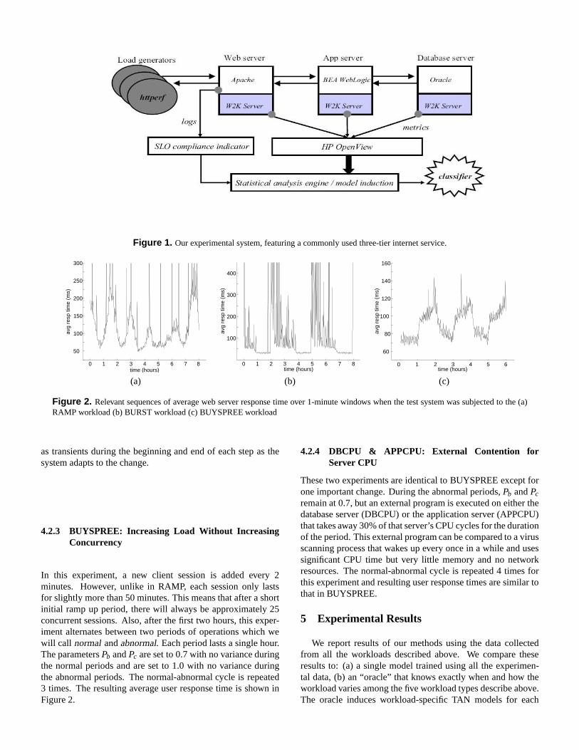
Figure 1. Our experimental system, featuring a commonly used three-tier internet service.

0 1 2 3 4 5 6 7 8

50

100

150

200

250

300

time (hours)

avg

resp

tim

e (m

s)

0 1 2 3 4 5 6 7 8

100

200

300

400

time (hours)

avg

resp

tim

e (m

s)

time (hours)av

g re

sp ti

me

(ms)

0 1 2 3 4 5 6

60

80

100

120

140

160

(a) (b) (c)

Figure 2. Relevant sequences of average web server response time over1-minute windows when the test system was subjected to the (a)RAMP workload (b) BURST workload (c) BUYSPREE workload

as transients during the beginning and end of each step as thesystem adapts to the change.

4.2.3 BUYSPREE: Increasing Load Without IncreasingConcurrency

In this experiment, a new client session is added every 2minutes. However, unlike in RAMP, each session only lastsfor slightly more than 50 minutes. This means that after a shortinitial ramp up period, there will always be approximately 25concurrent sessions. Also, after the first two hours, this exper-iment alternates between two periods of operations which wewill call normalandabnormal. Each period lasts a single hour.The parametersPb andPc are set to 0.7 with no variance duringthe normal periods and are set to 1.0 with no variance duringthe abnormal periods. The normal-abnormal cycle is repeated3 times. The resulting average user response time is shown inFigure 2.

4.2.4 DBCPU & APPCPU: External Contention forServer CPU

These two experiments are identical to BUYSPREE except forone important change. During the abnormal periods,Pb andPc

remain at 0.7, but an external program is executed on either thedatabase server (DBCPU) or the application server (APPCPU)that takes away 30% of that server’s CPU cycles for the durationof the period. This external program can be compared to a virusscanning process that wakes up every once in a while and usessignificant CPU time but very little memory and no networkresources. The normal-abnormal cycle is repeated 4 times forthis experiment and resulting user response times are similar tothat in BUYSPREE.

5 Experimental Results

We report results of our methods using the data collectedfrom all the workloads described above. We compare theseresults to: (a) a single model trained using all the experimen-tal data, (b) an “oracle” that knows exactly when and how theworkload varies among the five workload types describe above.The oracle induces workload-specific TAN models for each

type and invokes the appropriate model during testing; whileclearly unrealistic in a real system, this method provides aqual-itative indicator of the best we could do.

We learn the ensemble of models as described in Algorithm 1using a subset of the available data. The subset of data are thefirst 4-6 hours of each workload. We keep the last portion ofeach workload as a test (validation) set. Overall, the trainingset is 28 hours long (1680 samples) and the test set is 10 hourslong (600 samples). The training set starts with alternating twohour sequences of DBCPU, APPCPU, and BUYSPREE, withDBCPU and APPCPU represented three times and BUYSPREEtwice. This is followed by six hour sequences of data fromRAMP and BURST. The result is a training set which has fivedifferent workload conditions some of which are repeated sev-eral times. Testing on the test set with the ensemble amountsto the same steps as in Algorithm 1, except for the fact that theensemble is not initially empty (but has all the models trainedon the training data) and no new models are added at any point.The accuracies and metric attribution provided by this testingprocedure show how generalizable the models are on unseendata with similar types of workloads. The results of these testsare described below.

5.1 Accuracy

Table 1 shows the balanced accuracy (BA), false alarm anddetection rates, measured on the validation data, of our ap-proach compared to the single model and the set of modelstrained on each of the five workloads. We present results for theensemble of models with three different training window size(80, 120 and 240 samples). We see that for all cases: (a) theensemble’s performance with any window size is significantlybetter than the single-model, (b) the ensemble’s performance isrobust to wide variations of the training window size, and (c)the ensemble’s performance is slightly better, mainly in termsof detection rates, compared to the set of five individual modelstrained on each of the workload conditions we induced.

The last observation (c) is at first glance puzzling, as intu-ition suggests that the set of models trained specifically for eachworkload should perform best. However, some of the work-loads on the system were quite complex, e.g., BURST has aramp up of number of concurrent sessions over time and othervaried conditions. This complexity is further characterized inSection 5.3, where we will see that it takes many more samplesto capture patterns of the BURST workload, and with lower ac-curacy compared to the other workloads. The ensemble of mod-els, which is allowed to learn multiple models foreach work-load, is better able to characterize this complexity than the sin-gle model trained with the entire dataset of that workload.

The table also shows the total number of metrics includedin the models and the average number of metrics attributableto specific instances of SLO violations (as discussed in sec-tion 3.3). The ensemble chooses many more metrics overallbecause models are trained independently of each other, whichsuggests that there is some redundancy among the differentmodels in the ensemble. However, only a handful of metricsare attributed to each instance of an SLO violation, thereforeattribution is not affected by the redundancy.

Most of the single model’s false alarms occur for the

metrics avg attr BA FA Detchosen metrics

Ensemble W80 64 2.3 95.67 4.19 95.53Ensemble W120 52 2.5 95.12 4.84 95.19Ensemble W240 33 3.7 94.68 5.48 94.85

Workload 9 2 93.62 4.51 91.75specific modelsSingle model 4 2 86.10 21.61 93.81

Table 1. Summary of performance results. First three rowsshow results for ensemble of models with different size trainingwindow (80, 120, 240 samples).

BUYSPREE workload, and we observed that the lower falsealarm rate of the ensemble in these cases was largely attribut-able to the inclusion of three metrics that werenot chosen bythe single model, namely number of incoming packets and bytesto the application server and number of requests to the system.Additionally, the first two metrics also appear in the model spe-cific to the BUYSPREE workload. Thus, the ensemble of mod-els is capable of capturing more of the important patterns, bothof violations and non-violations by focusing on different met-rics for different workloads.

Adaptation to different workloads To show how the en-semble of models adapts to changing workloads, we store theaccuracy of the ensemble of models as the ensemble is trained.The changes in the ensemble’s accuracy as a function of thenumber of samples is shown in Figure 3a. There are initiallyno models in the ensemble until enough samples of violationsare observed. The ensemble’s accuracy remains high until newworkloads elicit behaviors different from those already seen,but adaptation is quick once enough samples of the new work-load have been seen. An interesting situation occurs duringadaptation for the last workload condition (BURST, marked as5 in the figure). We see that the accuracy decreases signifi-cantly when this workload condition first appears, but improvesafter about 100 samples. It then decreases again, illustratingthe complexity of this workload and the need for multiple mod-els to capture its behavior, and finally recovers as more sam-ples appear. It is worth noting that there is a tradeoff betweenadaptation speed and robustness of the models, e.g., with smalltraining window, adaptation would be fast, however, the modelsmight not be robust to overfitting and will not generalize to newdata.

We remind the reader that prediction accuracy is not a directevaluation of the proficiency of our approach. After all, SLOvi-olation can be determined by direct measurement, so there isnoneed to predict it from lower level metric data. However, theseraw accuracy figures do provide a quantitative assessment ofhow well the model(s) produced capture correlations betweenlow level metrics and SLO state. Intuitively, models that cap-ture system behavior patterns more faithfully should be morehelpful in diagnosing problems. Although we cannot rigorouslyprove that is the case, the next section will show anecdotal evi-dence that metric attribution using models induced according toour approach do point to the likely root cause of an issue.

5.2 Metric attribution

Figure 3b illustrates the metric attribution for part of thetestset for one of the ensemble of models we learned. The imageillustrates which metrics were implicated with an SLO viola-tion during the different workload conditions. For instances ofviolations in the BUYSPREE workload, network inbyte and in-packet are implicated with most of the instances of violation.In addition, due to the increased workload, the App server CPU(usertime) is sometimes also implicated with the SLO viola-tions, as the heavier workload causes increased CPU load. Forthe DBCPU workload, we see that the DB CPU is implicatedfor all instances of SLO violation, while for the APPCPU work-load, all the App server CPU is implicated with all SLO viola-tions. Some SLO violation instances in the APPCPU workloadalso implicate the network inbyte and inpacket, but what theimage does not show is that they are implicated because ofde-creasednetwork activity, in contrast to BUYSPREE in whichthey are implicated due toincreasednetwork activity. With theknowledge that the application server CPU load is high and thenetwork activity is low, a diagnosis of external contentionforthe CPU resource can be deduced.

It is worth noting that the image illustrates that for differentworkloads (hence different performance problem causes) thereappears to be different “signatures” of metric attribution— cat-aloguing such signatures could potentially serve as a basisforfast diagnosis based on information retrieval principals.

5.3 Learning surfaces: determining the appropriatesample size

To test how much data is needed to learn accurate models,we take the common approach of testing it empirically. Typi-cally, in most machine learning research, the size of the train-ing set is incrementally increased and accuracy is measuredona fixed test set. The result of such experiments are learningcurves, which typically show what is the minimum training dataneeded to achieve models that perform close to the maximumaccuracy possible. In the learning curve approach, the ratio be-tween violation and non-violation samples is kept fixed as thenumber of training samples is increased. Additionally, thetestset is usually chosen such that the ratio between the two classesis equivalent to the training data. These two choices can lead toan optimistic estimate of the number of samples needed in train-ing, because real applications (including ours) often exhibit amismatch between training and testing distribution and becauseit is difficult to keep the ratio between the classes fixed.

To obtain a more complete view of the amount of dataneeded, we use Forman and Cohen’s approach [15] and varythe number of violations and non-violations in the trainingsetindependently of each other, testing on a fixed test set that hasa fixed ratio between violations and no violations. The resultof this testing procedure is alearning surfacethat shows thebalanced accuracy as a function of the ratio of violations tonon-violations in the training set. Figure 3c shows the learn-ing surface for the RAMP workload we described in the previ-ous section. Each point in the learning surface is the averageof five different trials. Examining the learning surface revealsthat after about 80 samples of each class, we reach a plateau

Workload # vio # no vio max BA(%)RAMP 90 80 92.35BURST 180 60 81.85

BUYSPREE 40 40 95.74APPCPU 20 30 97.64DBCPU 20 20 93.90

Table 2. Minimum sample sizes needed to achieve accuracythat is at least 95% of the maximum accuracy achieved for eachworkload condition.

in the surface, indicating that increasing the number of sam-ples does not necessarily provide much higher accuracies. Thesurface also shows us that small numbers of violations pairedwith high numbers of nonviolations results in poor BA, eventhough the total number of samples is high; e.g., accuracy with200 nonviolations and 20 violations is only 75%, in contrasttoother combinations on the surface with the same total numberof samples (220) but significantly higher accuracy.

Table 2 summarizes the minimum number of samples neededfrom each class to achieve 95% of the maximum accuracy. Wesee that the simpler APPCPU and DBCPU workloads requirefewer samples of each class to reach this accuracy thresholdcompared to the more complex RAMP or BURST workloads.

In properly designed systems, contractual SLOs having se-rious repercussions are rarely violated. Therefore, it is likelythat very large windows of data would be needed to captureenough samples of violation to construct a model. However,as mentioned previously, larger windows increases the chancethat a single model tries to captures several disparate behav-ior patterns. This issue can be addressed by making a virtualSLO that is more stringent than what is contractually obligated.This would be useful in determine what factors may cause asystem to operate such that the real SLO is close to being vio-lated. Also, the high level indictor of system performance neednot be defined only in terms of throughput or latency, but couldalso be in terms of measures like a buy-to-browse ratio for ane-commerce site.

5.4 Summary of Results

The key observations of our results may be summarized asfollows:

1. Even when multiple workload-specific models are trainedon separate parts of the workload, the ensemble methodresults in higher accuracy because the ability to learn andmanage multiple models results in better characterizationof these complex workloads.

2. The ensemble method also gives better metric attribut-ion than workload-specific models, and allows us to ob-serve that different workloads seem to be characterized bymetric-attribution “signatures”. Future work may includeexploiting such distinct signatures for enhanced diagnosis.

3. The ensemble provides rapid adaptation to changing work-loads, but adaptation speed is sensitive not only to the

200 400 600 800 1000 1200 1400 16000.5

0.55

0.6

0.65

0.7

0.75

0.8

0.85

0.9

0.95

1

Time (minutes)

Ba

lan

ced

Acc

ura

cy

2 3 1 2 3 1 2 4 51

(a) (b) (c)

Figure 3. (a) Balanced accuracy of ensemble of models during training. Vertical dashed lines show boundaries between workload changes.Numbers above figure enumerate which of the five types of workload corresponds to each period (1=DBCPU, 2=APPCPU, 3=BUYSPREE,4=RAMP, 5=BURST). (b) Metric attribution image for the ensemble of models. First column is the actual SLO state (white indicatesviolation), other columns are the state of each metric chosen in the ensemble (white indicates the violation can be attributed to this metric).Y-axis is epochs (minutes), dark horizontal lines show boundaries between changes in workloads. (c) Learning surface for RAMP experimentshowing balanced accuracy. The color map on each figure showsthe mapping between color and accuracy. Each quad in the surface is thebalanced accuracy of the right bottom left corner of the quad.

number of samples seen but also the ratio between the twoclasses of samples (violation and nonviolation).

4. The observed overlap of the metrics chosen by variousmodels in the ensemble suggests that there is some redun-dancy among the models in the ensemble. One area offuture work will be to investigate and remove this redun-dancy.

5. Choosing a “winner take all” selection function rather thanone that combines models in the ensemble gives excellentresults; future work may include investigating more com-plicated selection functions or further refinements of met-ric attribution, such as ranking the metrics based on theiractual log-likelihood ratio difference values.

6. At no point in our process is explicit domain-specificknowledge required, though such knowledge could beused, e.g., to guide the selection of which metrics tocapture for model induction. Future work may investi-gate which aspects of our approach could be enhanced bydomain-specific knowledge.

6 Related Work

Automatic monitoring and dynamic adaptation of computersystems is a topic of considerable current interest, as evidencedby the recent spate of work in so-called “autonomic comput-ing”. Recent approaches to automatic resource allocation usefeedforward control [16], feedback control [17], and an open-market auction of cluster resources [18]. Our goal is to un-derstand the connection between high-level actionable prop-erties such as SLO’s, which drive these adaptation efforts,and the low-level properties that correspond to allocatable re-sources, decreasing the granularity of resource allocation deci-sions. Other complementary approaches pursuing similar goals

include WebMon [19] and Magpie [20]. Aguilera et al. [21]provide an excellent review of these and related research ef-forts, and propose algorithms to infer causal paths of messagesrelated to individual high-level requests or transactionsto helpdiagnose performance problems.

Pinpoint [6] uses anomaly-detection techniques to infer fail-ures that might otherwise escape detection in componentizedapplications. The authors of that work observed that some iden-tical components have distinct behavioral modes that depend onwhich machine in a cluster they are running on. They addressedthis by explicitly adding human-level information to the modelinduction process, but approaches such as ours could be appliedfor automatic detection of such conditions and disqualificationof models that try to capture a “nonexistent average” of multi-ple modes. Similarly, Mesnier et al. [22] find that decision treescan accurately predict properties of files (e.g., access patterns)based on creation-time attributes, but that models from onepro-duction environment may not be well-suited to other environ-ments, inviting exploration of an adaptive approach.

Whereas “classic” approaches to performance modeling andanalysis [23] rely ona priori knowledge from human experts,our techniques induce performance models automatically frompassive measurements alone. Other approaches perform diag-nosis using expert systems based on low-level metrics [24];such approaches are prone to both false negatives (low-level in-dicators do not trigger any rule even when high-level behavioris unacceptable) and false negatives (low-level indicators trig-ger rules when there is no problem with high-level behavior). Incontrast, our correlation-based approach uses observablehigh-level behavior as the “ground truth”, and our models are in-duced and updated automatically, allowing for rapid adaptationto a changing environment.

7 Conclusion

We routinely build and deploy systems whose behavior weunderstand only at a very coarse grain. Although this obser-vation motivates autonomic computing, progress requires thatwe be able to characterize actionable system behaviors in termsof lower-level system properties. Furthermore, previous effortsshowed that no single low-level metric is a good predictor ofhigh-level behaviors. Our contribution has been to extend oursuccessful prior work on using TAN (Bayesian network) modelscomprising low-level measurements both for prediction of com-pliance with service-level objectives and for metric attribution(understanding which low-level properties are correlatedwithSLO compliance or noncompliance). Specifically, by manag-ing an ensemble of such models rather than a single model, weachieve rapid adaptation of the model to changing workloads,infrastructure changes, and external disturbances. The result isthe ability to continuously characterize a key high-level behav-ior of our system (SLO compliance) in terms of multiple low-level properties; this gives the administrator, whether human ormachine, a narrow focus in considering repair or recovery ac-tions. Using a real system under realistic workloads, we showedthat collecting instrumentation, inducing models, and maintain-ing the ensemble of models is inexpensive enough to do in (soft)real time. Beyond the specific application of TAN models inour own work, we believe our approach to managing ensem-bles of models will prove more generally useful to the rapidly-growing community of researchers applying machine learningtechniques to issues of system dependability.

8 Acknowledgments

We thank Terence Kelly for his help in generating the work-loads. Rob Powers and Peter Bodík provided useful commentson a previous version of this paper. Finally, the comments ofthe reviewers and our shepherd greatly improved the presenta-tion of the material.

References

[1] I. Cohen, M. Goldszmidt, T. Kelly, J. Symons, and J. Chase,“Correlating instrumentation data to system states: A buildingblock for automated diagnosis and control,” in6th Symposium onOperating Systems Design and Implementation (OSDI’04), Dec.2004.

[2] J. Pearl,Probabilistic Reasoning in Intelligent Systems: Networksof Plausible Inference. Morgan Kaufmann, 1988.

[3] N. Friedman, D. Geiger, and M. Goldszmidt, “Bayesian networkclassifiers,”Machine Learning, vol. 29, pp. 131–163, 1997.

[4] G. Brier, “Verification of forecasts expressed in terms of proba-bility,” Monthly weather review, vol. 78, no. 1, pp. 1–3, 1950.

[5] I. Cohen and M. Goldszmidt, “Properties and benefits of cal-ibrated classifiers,” in8th European Conference on Principlesand Practice of Knowledge Discovery in Databases (PKDD),pp. 125–136, Sept. 2004.

[6] E. Kıcıman and A. Fox, “Detecting application-level failures incomponent-based internet services.” Submitted for publication,September 2004.

[7] R. Duda, P. Hart, and D. Stork,Pattern Classification. New York:John Wiley and Sons, 2001.

[8] R. Kohavi and G. H. John, “Wrappers for feature subset selec-tion,” Artificial Intelligence, vol. 97, no. 1-2, pp. 273–324, 1997.

[9] R. Kohavi, “A study of cross-validation and bootstrap for accu-racy estimation and model selection,” inInternational Joint Con-ference on Artificial Intelligence (IJCAI), pp. 1137–1145, 1995.

[10] L. Breiman, “Bagging predictors,”Machine Learning, vol. 24,no. 2, pp. 123–140, 1996.

[11] R. Caruana, A. Niculescu-Mizil, G. Crew, and A. Ksikes,“En-semble selection from libraries of models,” inInternational con-ference on Machine learning ICML, 2004.

[12] P. Domingos, “Bayesian averaging of classifiers and theoverfit-ting problem,” inInternational Conference on Machine LearningICML, pp. 223–230, 2000.

[13] A. Messinger, “Personal comm..” BEA Systems, 2004.

[14] S. Duvur, “Personal comm..” Sun Microsystems, 2004.

[15] G. Forman and I. Cohen, “Learning from little: Comparison ofclassifiers given little training,” in8th European Conference onPrinciples and Practice of Knowledge Discovery in Databases(PKDD), pp. 161–172, Sept. 2004.

[16] E. Lassettre, D. Coleman, Y. Diao, S. Froelich, J. Hellerstein,L. Hsiung, T. Mummert, M. Raghavachari, G. Parker, L. Rus-sell, M. Surendra, V. Tseng, N. Wadia, and P. Ye, “DynamicSurge Protection: An Approach to Handling Unexpected Work-load Surges with Resource Actions that have Lead Times,” inProc. of 1st Workshop on Algorithms and Architectures for Self-Managing Systems, (San Diego, CA), June 2003.

[17] S. Parekh, N. Gandhi, J. Hellerstein, D. Tilbury, T. Jayram, andJ. Bigus, “Using control theory to achieve service level objec-tives in performance management,”Real Time Systems Journal,vol. 23, no. 1–2, 2002.

[18] K. Coleman, J. Norris, A. Fox, and G. Candea, “OnCall: Defeat-ing spikes with a free-market server cluster,” inProc. Interna-tional Conference on Autonomic Computing, (New York, NY),May 2004.

[19] P. K. Garg, M. Hao, C. Santos, H.-K. Tang, and A. Zhang, “Webtransaction analysis and optimization,” Tech. Rep. HPL-2002-45,Hewlett-Packard Labs, Mar. 2002.

[20] P. Barham, R. Isaacs, R. Mortier, and D. Narayanan, “Mag-pie: real-time modelling and performance-aware systems,”inProc. 9th Workshop on Hot Topics in Operating Systems, (Lihue,Hawaii), June 2003.

[21] M. K. Aguilera, J. C. Mogul, J. L. Wiener, P. Reynolds, andA. Muthitacharoen, “Performance debugging for distributed sys-tems of black boxes,” inProc. 19th ACM Symposium on Operat-ing Systems Principles, (Bolton Landing, NY), 2003.

[22] M. Mesnier, E. Thereska, G. R. Ganger, D. Ellard, and M. Seltzer,“File classification in self-* storage systems,” inProceedingsof the First International Conference on Autonomic Computing(ICAC-04), May 2004.

[23] R. Jain,The Art of Computer Systems Performance Analysis:Techniques for Experimental Design, Measurement, Simulation,and Modeling. New York, NY: Wiley-Interscience, 1991.

[24] A. Cockcroft and R. Pettit,Sun Performance and Tuning. Pren-tice Hall, 1998.