Automated Prostate Cancer Diagnosis and Gleason Grading of Tissue Microarrays

Ali Tabesh1,2, Vinay P. Kumar1, Ho-Yuen Pang1, David Verbel1, Angeliki Kotsianti1, Mikhail Teverovskiy1,*, and Olivier Saidi1

1 Aureon Biosciences Corporation, Yonkers, NY 10701 2 ECE Department, The University of Arizona, Tucson, AZ 85721

ABSTRACT

We present the results on the development of an automated system for prostate cancer diagnosis and Gleason grading. Images of representative areas of the original Hematoxylin-and-Eosin (H&E)-stained tissue retrieved from each patient, either from a tissue microarray (TMA) core or whole section, were captured and analyzed. The image sets consisted of 367 and 268 color images for the diagnosis and Gleason grading problems, respectively. In diagnosis, the goal is to classify a tissue image into tumor versus non-tumor classes. In Gleason grading, which characterizes tumor aggressiveness, the objective is to classify a tissue image as being from either a low- or high-grade tumor. Several feature sets were computed from the image. The feature sets considered were: (i) color channel histograms, (ii) fractal dimension features, (iii) fractal code features, (iv) wavelet features, and (v) color, shape and texture features computed using Aureon Biosciences' MAGIC™ system. The linear and quadratic Gaussian classifiers together with a greedy search feature selection algorithm were used. For cancer diagnosis, a classification accuracy of 94.5% was obtained on an independent test set. For Gleason grading, the achieved accuracy of classification into low- and high-grade classes of an independent test set was 77.6%.

Keywords: Prostate cancer, automated cancer diagnosis, automated Gleason grading, tissue image processing, tissue image segmentation, fractal dimension, fractal codes, wavelets, feature selection, statistical classification.

1. INTRODUCTION

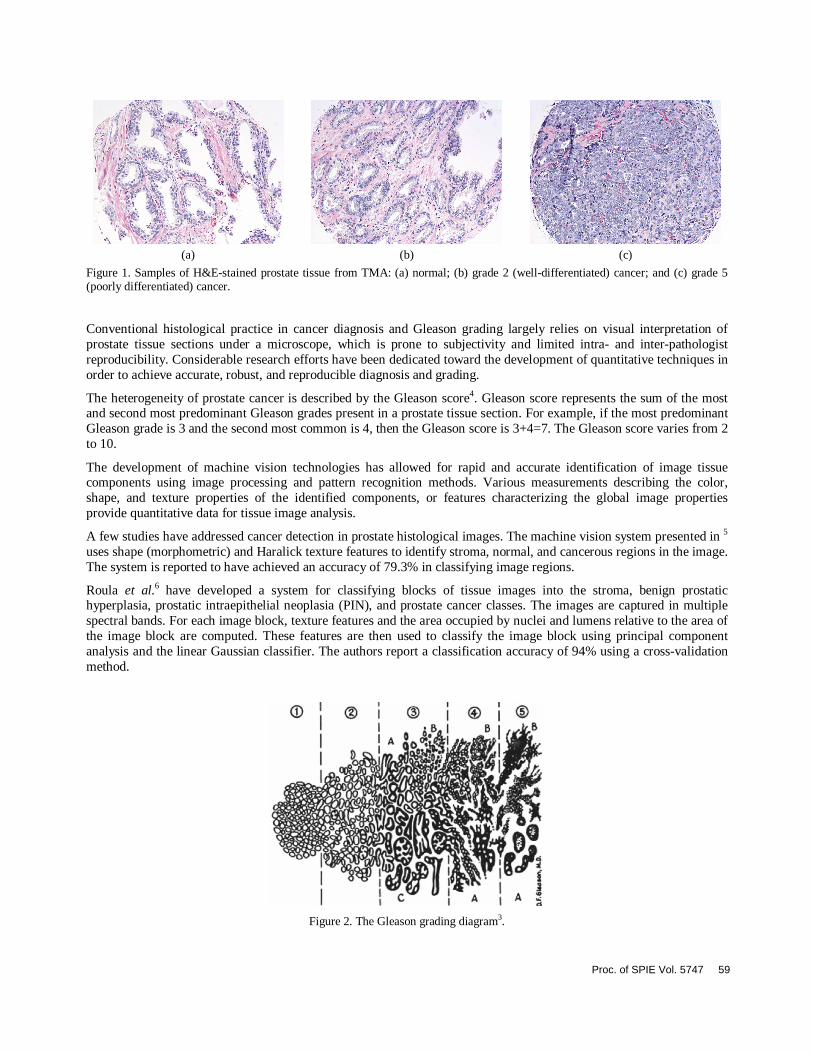
Prostate cancer is the most prevalent form of cancer and the second most common cause of death among men in the United States1. Several screening methodologies exist for prostate cancer diagnosis. One of the most reliable methods is the examination of histological specimens under the microscope by a pathologist. Diagnosis of prostate cancer is carried out by examining the glandular architecture of the specimen. Normal prostate tissue (Figure 1(a)) consists of gland units surrounded by fibromuscular tissue, called stroma, which holds the gland units together. Each gland unit is made of a row of epithelial cells located around a circularly shaped “hole” in the tissue, named the lumen. When cancer occurs, epithelial cells replicate in an uncontrolled way, disrupting regular arrangement of the gland units. As shown in Figure 1(c), the lumens have been filled with epithelial cells and stroma has virtually disappeared.

The aggressiveness of the cancerous tissue is quantified through histological grading. Histological grading is valuable to physicians in several ways. First, it aids with identifying the extent of the disease. Second, cancer grade correlates well with patient survival. Finally, knowledge of cancer grade helps with determining the most appropriate treatment options2.

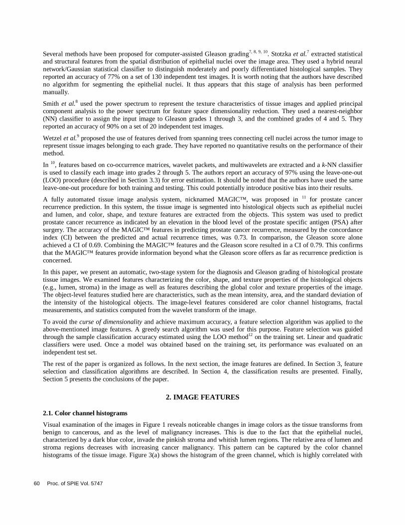
The most common method for histological grading of prostate tissue is the Gleason grading system3. In this system, depicted in Figure 2, the tissue is classified into five grades, numbered 1 through 5. The grade increases with increasing malignancy level and cancer aggressiveness. Gleason grade characterizes tumor differentiation, i.e., the degree of tumor resemblance to normal tissue. Grade 1 corresponds to well-differentiated tissue, i.e., tissue with the highest degree of resemblance to normal tissue, and indicates a high chance of patient survival, and grade 5 corresponds to poorly differentiated tissue, and indicates a low chance of survival.

* mikhail.teverovskiy@aureon.com; phone: 1-914-377-4022; fax: 1-914-377-4001; www.aureon.com.

Medical Imaging 2005: Image Processing, edited by J. Michael Fitzpatrick,Joseph M. Reinhardt, Proc. of SPIE Vol. 5747 (SPIE, Bellingham, WA, 2005)

1605-7422/05/$15 · doi: 10.1117/12.597250

58

(a) (b) (c)

Figure 1. Samples of H&E-stained prostate tissue from TMA: (a) normal; (b) grade 2 (well-differentiated) cancer; and (c) grade 5 (poorly differentiated) cancer.

Conventional histological practice in cancer diagnosis and Gleason grading largely relies on visual interpretation of prostate tissue sections under a microscope, which is prone to subjectivity and limited intra- and inter-pathologist reproducibility. Considerable research efforts have been dedicated toward the development of quantitative techniques in order to achieve accurate, robust, and reproducible diagnosis and grading.

The heterogeneity of prostate cancer is described by the Gleason score4. Gleason score represents the sum of the most and second most predominant Gleason grades present in a prostate tissue section. For example, if the most predominant Gleason grade is 3 and the second most common is 4, then the Gleason score is 3+4=7. The Gleason score varies from 2 to 10.

The development of machine vision technologies has allowed for rapid and accurate identification of image tissue components using image processing and pattern recognition methods. Various measurements describing the color, shape, and texture properties of the identified components, or features characterizing the global image properties provide quantitative data for tissue image analysis.

A few studies have addressed cancer detection in prostate histological images. The machine vision system presented in 5 uses shape (morphometric) and Haralick texture features to identify stroma, normal, and cancerous regions in the image. The system is reported to have achieved an accuracy of 79.3% in classifying image regions.

Roula et al.6 have developed a system for classifying blocks of tissue images into the stroma, benign prostatic hyperplasia, prostatic intraepithelial neoplasia (PIN), and prostate cancer classes. The images are captured in multiple spectral bands. For each image block, texture features and the area occupied by nuclei and lumens relative to the area of the image block are computed. These features are then used to classify the image block using principal component analysis and the linear Gaussian classifier. The authors report a classification accuracy of 94% using a cross-validation method.

Figure 2. The Gleason grading diagram3.

Proc. of SPIE Vol. 5747 59

Several methods have been proposed for computer-assisted Gleason grading7, 8, 9, 10. Stotzka et al.7 extracted statistical and structural features from the spatial distribution of epithelial nuclei over the image area. They used a hybrid neural network/Gaussian statistical classifier to distinguish moderately and poorly differentiated histological samples. They reported an accuracy of 77% on a set of 130 independent test images. It is worth noting that the authors have described no algorithm for segmenting the epithelial nuclei. It thus appears that this stage of analysis has been performed manually.

Smith et al.8 used the power spectrum to represent the texture characteristics of tissue images and applied principal component analysis to the power spectrum for feature space dimensionality reduction. They used a nearest-neighbor (NN) classifier to assign the input image to Gleason grades 1 through 3, and the combined grades of 4 and 5. They reported an accuracy of 90% on a set of 20 independent test images.

Wetzel et al.9 proposed the use of features derived from spanning trees connecting cell nuclei across the tumor image to represent tissue images belonging to each grade. They have reported no quantitative results on the performance of their method.

In 10, features based on co-occurrence matrices, wavelet packets, and multiwavelets are extracted and a k-NN classifier is used to classify each image into grades 2 through 5. The authors report an accuracy of 97% using the leave-one-out (LOO) procedure (described in Section 3.3) for error estimation. It should be noted that the authors have used the same leave-one-out procedure for both training and testing. This could potentially introduce positive bias into their results.

A fully automated tissue image analysis system, nicknamed MAGIC™, was proposed in 11 for prostate cancer recurrence prediction. In this system, the tissue image is segmented into histological objects such as epithelial nuclei and lumen, and color, shape, and texture features are extracted from the objects. This system was used to predict prostate cancer recurrence as indicated by an elevation in the blood level of the prostate specific antigen (PSA) after surgery. The accuracy of the MAGIC™ features in predicting prostate cancer recurrence, measured by the concordance index (CI) between the predicted and actual recurrence times, was 0.73. In comparison, the Gleason score alone achieved a CI of 0.69. Combining the MAGIC™ features and the Gleason score resulted in a CI of 0.79. This confirms that the MAGIC™ features provide information beyond what the Gleason score offers as far as recurrence prediction is concerned.

In this paper, we present an automatic, two-stage system for the diagnosis and Gleason grading of histological prostate tissue images. We examined features characterizing the color, shape, and texture properties of the histological objects (e.g., lumen, stroma) in the image as well as features describing the global color and texture properties of the image. The object-level features studied here are characteristics, such as the mean intensity, area, and the standard deviation of the intensity of the histological objects. The image-level features considered are color channel histograms, fractal measurements, and statistics computed from the wavelet transform of the image.

To avoid the curse of dimensionality and achieve maximum accuracy, a feature selection algorithm was applied to the above-mentioned image features. A greedy search algorithm was used for this purpose. Feature selection was guided through the sample classification accuracy estimated using the LOO method12 on the training set. Linear and quadratic classifiers were used. Once a model was obtained based on the training set, its performance was evaluated on an independent test set.

The rest of the paper is organized as follows. In the next section, the image features are defined. In Section 3, feature selection and classification algorithms are described. In Section 4, the classification results are presented. Finally, Section 5 presents the conclusions of the paper.

2. IMAGE FEATURES

2.1. Color channel histograms

Visual examination of the images in Figure 1 reveals noticeable changes in image colors as the tissue transforms from benign to cancerous, and as the level of malignancy increases. This is due to the fact that the epithelial nuclei, characterized by a dark blue color, invade the pinkish stroma and whitish lumen regions. The relative area of lumen and stroma regions decreases with increasing cancer malignancy. This pattern can be captured by the color channel histograms of the tissue image. Figure 3(a) shows the histogram of the green channel, which is highly correlated with

60 Proc. of SPIE Vol. 5747

image brightness, for the images depicted in Figure 1. It can be observed that there are far more bright pixels in the normal image than in the cancerous images. Moreover, the number of bright pixels decreases as the Gleason grade increases from 2 to 5.

Figure 3(b) shows the histograms of the difference between the values in the red and blue channels for the images in Figure 1. Epithelial (and other) nuclei are characterized by large negative values of the difference between red and blue channels. The histograms indicate that for the normal tissue image there are fewer pixels with large negative values than for the cancerous images. As the Gleason grade increases, the number of such pixels rises.

The white pixels in prostate tissue images represent not only lumen but also background and artifacts caused by broken tissue structure. In order to eliminate the effect of such white pixels from histogram analysis, the histograms of the tissue images were considered both before and after removing white pixels. White pixels were detected via simple thresholding. This was accomplished by first transforming the image from the RGB space into the YCbCr space, and then applying a threshold to the luminance (Y) component.

0 50 100 150 200 2500

1

2

3

4

5

6

7

8x 10

5

intensity in green channel

num

ber

of p

ixel

s

normalgrade 2grade 5

-300 -200 -100 0 100 200 3000

2

4

6

8

10

12 x 105

difference between intensity in red and blue channels

num

ber

of p

ixel

s

normalgrade 2grade 5

(a) (b)

Figure 3. (a) Histogram of the intensity of the green color channel for the images in Figure 1; (b) histogram of the difference between the intensities of the red and blue channels.

2.2. Texture features

The images in Figure 1 exhibit a change in texture as the tissue progresses towards malignancy. The most visible change is that the texture becomes more uniform as the epithelial nuclei spread across the tissue. Several feature sets were computed to capture the texture characteristics of the tissue image.

2.2.1. Fractal dimension features

Fractal geometry provides a tool for quantitative description of complex, irregularly shaped objects in pathological images. A detailed review of the use of fractal geometry in pathology may be found in 13. A common fractal property of an object is its fractal dimension. The fractal dimension provides a quantitative measure of the space-filling capacity of an object. For instance, the fractal dimension of a straight line is the same as its topological dimension, i.e., 1, since it can only fill a one-dimensional sub-space. But for a more complex curve, the fractal dimension can be fractional and therefore different from its topological dimension. For a detailed description of the fractal dimension and methods of its calculation, see 13, 14.

To obtain fractal dimension features, the tissue image is thresholded at bN fixed, equally spaced thresholds in each of

its color channels, resulting in bN3 binary images (Figure 4). For each binary image ikB , obtained by applying the k-th

threshold to the i-th channel, a fractal dimension value ikγ is computed. The box counting algorithm13, 14 is used for

fractal dimension calculation. The values ikγ , 3,2,1=i , bNk ,...,1= are put together to form the bN3 -dimensional

feature vector [ ]331

221

111 , ,, , ,, , ,

bbb NNN γγγγγγ KKK=γ . The vector γ provides a fractal representation of the image to be

analyzed.

Proc. of SPIE Vol. 5747 61

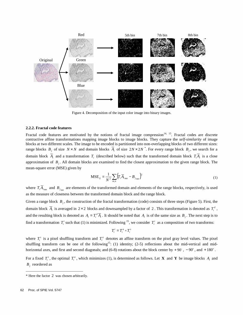
Figure 4. Decomposition of the input color image into binary images.

2.2.2. Fractal code features

Fractal code features are motivated by the notions of fractal image compression14, 15. Fractal codes are discrete contractive affine transformations mapping image blocks to image blocks. They capture the self-similarity of image blocks at two different scales. The image to be encoded is partitioned into non-overlapping blocks of two different sizes: range blocks jB of size NN × and domain blocks iA of size NN 22 × *. For every range block jB , we search for a

domain block iA and a transformation iT (described below) such that the transformed domain block ii AT is a close

approximation of jB . All domain blocks are examined to find the closest approximation to the given range block. The

mean-square error (MSE) given by

( )∑ −=nm

mnjmniiij BATN ,

2

2

1MSE (1)

where mnii AT and mnjB are elements of the transformed domain and elements of the range blocks, respectively, is used

as the measure of closeness between the transformed domain block and the range block.

Given a range block jB , the construction of the fractal transformation (code) consists of three steps (Figure 5). First, the

domain block iA is averaged in 22 × blocks and downsampled by a factor of 2 . This transformation is denoted as diT ,

and the resulting block is denoted as id

ii ATA = . It should be noted that iA is of the same size as jB . The next step is to

find a transformation tiT such that (1) is minimized. Following 15, we consider t

iT as a composition of two transforms:

si

ai

ti TTT o=

where siT is a pixel shuffling transform and a

iT denotes an affine transform on the pixel gray level values. The pixel shuffling transform can be one of the following15: (1) identity; (2-5) reflections about the mid-vertical and mid-

horizontal axes, and first and second diagonals; and (6-8) rotations about the block center by o90+ , o90− , and o180+ .

For a fixed siT , the optimal a

iT , which minimizes (1), is determined as follows. Let X and Y be image blocks iA and

jB reordered as

* Here the factor 2 was chosen arbitrarily.

Red

Green

Blue

5th bin 7th bin 8th bin

Original

62 Proc. of SPIE Vol. 5747

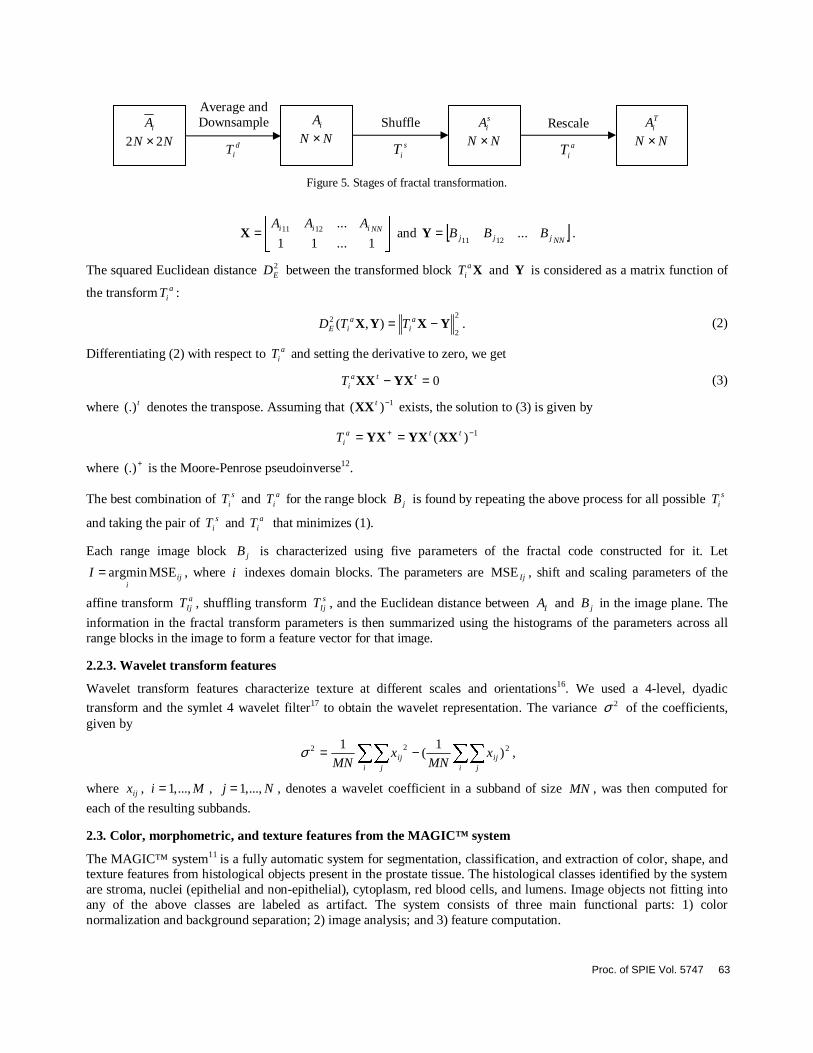
Figure 5. Stages of fractal transformation.

=

1...11

...1211 NNiii AAAX and [ ]

NNjjj BBB ...1211

=Y .

The squared Euclidean distance 2ED between the transformed block Xa

iT and Y is considered as a matrix function of

the transform aiT :

2

2

2 ),( YXYX −= ai

aiE TTD . (2)

Differentiating (2) with respect to aiT and setting the derivative to zero, we get

0=− ttaiT YXXX (3)

where t(.) denotes the transpose. Assuming that 1)( −tXX exists, the solution to (3) is given by

1)( −+ == ttaiT XXYXYX

where +(.) is the Moore-Penrose pseudoinverse12.

The best combination of siT and a

iT for the range block jB is found by repeating the above process for all possible siT

and taking the pair of siT and a

iT that minimizes (1).

Each range image block jB is characterized using five parameters of the fractal code constructed for it. Let

iji

I MSEargmin= , where i indexes domain blocks. The parameters are IjMSE , shift and scaling parameters of the

affine transform aIjT , shuffling transform s

IjT , and the Euclidean distance between IA and jB in the image plane. The

information in the fractal transform parameters is then summarized using the histograms of the parameters across all range blocks in the image to form a feature vector for that image.

2.2.3. Wavelet transform features

Wavelet transform features characterize texture at different scales and orientations16. We used a 4-level, dyadic

transform and the symlet 4 wavelet filter17 to obtain the wavelet representation. The variance 2σ of the coefficients, given by

222 )1

(1

∑∑∑∑ −=i j

iji j

ij xMN

xMN

σ ,

where ijx , Mi ...,,1= , Nj ...,,1= , denotes a wavelet coefficient in a subband of size MN , was then computed for

each of the resulting subbands.

2.3. Color, morphometric, and texture features from the MAGIC™ system

The MAGIC™ system11 is a fully automatic system for segmentation, classification, and extraction of color, shape, and texture features from histological objects present in the prostate tissue. The histological classes identified by the system are stroma, nuclei (epithelial and non-epithelial), cytoplasm, red blood cells, and lumens. Image objects not fitting into any of the above classes are labeled as artifact. The system consists of three main functional parts: 1) color normalization and background separation; 2) image analysis; and 3) feature computation.

iA

NN 22 ×

iA NN ×

siA NN ×

TiA NN ×

Average and Downsample

diT

Rescale

aiT

Shuffle

siT

Proc. of SPIE Vol. 5747 63

Color normalization is a pre-processing operation aimed at reducing color variations in H&E-stained tissue images, which arise from different staining and lighting conditions during image capture, and which can potentially affect segmentation accuracy. In the MAGIC™ system, color normalization is achieved by histogram matching18 to a reference image. This operation puts image colors in approximately the same range and thus reduces color variations.

For images acquired from TMA cores, the tissue area should be segmented from the background prior to tissue image analysis. The background corresponds to the transparent regions at the corners of the images in Figure 1. Background separation was carried out via intensity thresholding and a convex hull operation.

Image analysis is a multistage process based on an object oriented multiresolution image segmentation technique19. The first stage of processing consists of segmenting the image into small groups of contiguous pixels known as image objects. Objects are obtained by a region-growing algorithm which finds contiguous regions based on color similarity and shape regularity. The size of the resulting objects can be varied by adjusting a few control parameters. In the MAGIC™ system, objects rather than pixels are the smallest units on which image processing operations and feature calculations are performed. For example, when a threshold is applied to the image intensity, the object intensities, computed as the average intensity over all pixels belonging to each object, are subjected to the threshold. The image objects obtained in the first stage form a basic level 1 constituting the smallest scale of processing. Based on this level, subsequent higher (and coarser) levels are built by forming larger objects by combining the smaller ones in the lower levels. Thus, the objects form a network where the higher level objects “know” their sub-objects on the lower levels, which in turn are associated with their super-objects on the higher levels.

Level 2 of segmentation consists of re-segmenting the level 1 objects into coarse objects in order to classify them into meaningful histological classes. A series of rules based on color and neighborhood information were used for object classification. White space objects represent lumens and artifacts (broken tissue areas). Thresholding based on green (G) channel values was found to be sufficient for identifying white space objects.

Red blood cells do not absorb the H&E stain and thus have a low blue (B) channel value. Moreover, they are located inside blood vessels which appear as white space objects in the image. Thus, they are expected to have white space objects as their neighbors. Given the above observations, an object was classified as red blood cell if rbctBB < and

wstws ll > , where rbctB and wstl are fixed thresholds, and wsl is the border length of the object with the white space class. The border length between an object and its neighboring objects is defined as the sum of the lengths of the edges that the object shares with its neighbors. The object border length to a given class is the sum of the border lengths that the object shares with neighboring objects of that class.

The characteristic feature of nuclei in H&E-stained images is that they are stained blue compared to the rest of the histological objects. The difference between intensity of the red (R) and blue (B) channel BRd −= and the length/width ratio ρ of the object were found to be the best distinguishing features for the identification of nuclei

objects. An object was classified as nuclei object if Ndd < and Nρρ < , where ND and Nρ are fixed thresholds.

The tissue stroma is dominated by the color red. The intensity difference d , “red ratio” ( )BGRRr ++= , and the red

channel standard deviation Rσ of image objects were found to be the best features for the classification of stroma objects. An object is classified as stroma if it satisfies the following conditions:

SDd > , RR Σ<σ and Krf >)(

where SD , RΣ , and K are fixed thresholds, and )(rf is the quadratic Gaussian classifier given by (4) in Section 3.2. The classifier addresses a two-class (“stroma” (class 1) vs. “non-stroma” (class 2)) problem assuming that r for both classes follows a Gaussian distribution. The means and variances of the class-conditional distributions were estimated based on true stroma and non-stroma objects extracted from a tissue image labeled by a trained pathologist. As the Gaussian assumption is difficult to verify, the constant threshold K is introduced to account for the non-normality of the data12.

The above classification process captures only part of the nuclei and stroma objects. An iterative process is used to identify all stroma and nuclei objects. The process consists of alternatively classifying stroma followed by classifying

nuclei objects. Iteration begins by initializing two threshold values 0Sℜ and 0

Sℜ , for stroma and nuclei classification,

64 Proc. of SPIE Vol. 5747

respectively. At iteration k , the thresholds are updated as ∆−ℜ=ℜ −1kS

kS and ∆+ℜ=ℜ −1k

NkN , where ∆ is a constant.

If an unclassified object borders objects already identified as nuclei and kNr ℜ< , the object is classified as nuclei. If the

object has stroma objects as its immediate neighbors and kSr ℜ> , the object is labeled as stroma. The object remains

unclassified if neither of the conditions is satisfied. The process ends when no objects are left unclassified.

In the next stage, white space objects are classified as lumen or artifact (broken tissue areas). If a white space object satisfies the condition tnnn lll > , it is classified as lumen, where nl and nnl denote the length of the border line of the

object with the neighboring nuclei and non-nuclei objects, respectively, and tl is a fixed threshold. If the above condition is not satisfied, the white space object is labeled as artifact.

Objects classified as nuclei region often encompass multiple nuclei, and possibly surrounding cytoplasm. These fused nuclei areas need to be split into individual nuclei and cytoplasm objects. For this purpose, the classified nuclei objects are converted to the smaller sub-objects of level 1. If a sub-object meets the conditions NRR < and Nbb > , where

( )BGRBb ++= is the “blue ratio”, and NR and Nb are fixed thresholds, it remains a nuclei sub-object; otherwise it is classified as cytoplasm region sub-object. A region growing algorithm fuses the nuclei sub-objects constituting nuclei area under shape (roundness) constraints.

The input image contains different kinds of nuclei: epithelial nuclei, fibroblasts, basal nuclei, endothelial nuclei, apoptotic (dead) nuclei and red blood cells. Epithelial nuclei are the most important type of nuclei for cancer assessment. We classify the nuclei as being either epithelial or non-epithelial. Spatial relations between the tissue objects and nuclei morphometric features are used for epithelial vs. non-epithelial classification. Nuclei objects satisfying 2tc lll > are classified as epithelial nuclei, where cl is the border length to cytoplasm objects, l is the total

border length, and 2tl is a fixed threshold. If a nuclei object with Nρρ < and 2NRR < borders a stroma region, where

Nρ and 2NR are fixed thresholds, it is classified as non-epithelial nuclei. If some of these conditions are not satisfied it is categorized as a stroma region object. The classification of the image objects into valid histological objects completes the tissue image analysis.

The MAGIC™ features are calculated from various measurements associated with the objects obtained from the image analysis stage. These measurements include color (e.g., brightness), morphometric (e.g., area) and texture (channel standard deviation) properties. The MAGIC™ features for a given tissue image were computed as the various statistics (e.g., mean, standard deviation, minimum and maximum) of the different measurements associated with each object class. For example, for the class “lumen” and for the measurement type area, the MAGIC™ features are the mean, the standard deviation, the minimum and the maximum of the areas of all objects identified as lumen.

3. FEATURE SELECTION AND CLASSIFICATION

Two important stages in any pattern recognition system are feature selection and classification. Feature selection (FS) is the process of choosing a small subset of features (measurements) that are most relevant to the classification task, from a large set of available features. Classification is the statistical process of assigning a label to a sample from a finite set of labels. In this section, we review the feature selection and classification algorithms used in tumor/non-tumor image classification and Gleason grading.

3.1. Feature selection

FS has two benefits. It reduces the computational cost of recognition and it usually improves classification accuracy by mitigating the effect of the “curse of dimensionality”19. All FS algorithms are characterized by two traits12. The first is the optimality criterion J with respect to which we evaluate the quality of a feature subset. In our experiments J was selected as the classification accuracy estimated using the leave-one-out (LOO) procedure described in Section 3.3.

The second characteristic is a search strategy used to find a locally or globally optimal feature combination. In exhaustive search (ES), the globally optimal subset of features is found by evaluating all possible feature combinations. ES search is often computationally infeasible. Instead, greedy strategies are used that add or remove features from the feature subset in a stepwise fashion. The sequential forward search (SFS) algorithm is an example of this approach12.

Proc. of SPIE Vol. 5747 65

The SFS algorithm begins with selecting the individual feature that maximizes J . Each consequent stage of the algorithm consists of augmenting the set of already selected features with a new feature such that the resulting feature subset maximizes J . The process of adding new features is continued until J reaches a maximum.

3.2. Classification

Statistical classifiers fall into two general categories of parametric and non-parametric methods. Parametric methods rely on the assumption that the functional form of class-conditional distributions are known (e.g., Gaussian), whereas non-parametric methods make minimal assumptions about the form of the distributions. The choice of the classifier type depends on the sample size and the prior knowledge about the distribution of the features. In our studies, we focused on the use of parametric methods.

Statistical classifier used is a Bayesian two class classifier with zero-one loss function. We assumed that the class-conditional distributions of the classes follow the normal (Gaussian) density. With this assumption, the Bayes decision rule )(Xf is a quadratic function of the feature vector X given by12

2

1

2

12

1221

111 ln

||||

ln)()()()()(P

Pf TT −+−−−−−= −−

Σ

ΣµXΣµXµXΣµXX (4)

where iP , iµ , iΣ are the prior probability, mean, and covariance matrix of class i , 2,1=i , respectively, and |.|

denotes matrix determinant. For identical covariance matrices ΣΣΣ == 21 , (4) simplifies to a linear function given by

2

12

121

11

112 ln)(

2

1)()(

P

Pf TTT −Σ−Σ+Σ−= −−−

µµµµXµµX (5)

We refer to the classifiers given by (4) and (5) as quadratic and linear, respectively. The Bayesian decision rule is as follows. Decide class 1, if 0)( <Xf ; decide class 2, if 0)( >Xf ; and pick a class at random if 0)( =Xf .

3.3. Error estimation

For a given classifier and a dataset to be classified, the sample classification accuracy aP̂ is estimated as NNP ca =ˆ ,

where cN denotes the number of correctly classified samples and N is the total number of samples in the dataset. Two related performance measures often used in detection tasks are sensitivity and specificity. Let class 0 and class 1 correspond to the absence and presence of disease (or a lower or higher degree of disease) and let iN be the number of

patients in class i , 1,0=i . Moreover, let ijN , 1,0=i , 1,0=j , denote the number of patients in class i classified into

class j . Sample sensitivity SEP̂ is defined as 111 /ˆ NNPSE = and sample specificity SPP̂ is defined as 000 /ˆ NNPSP = .

We have used the following methods for splitting the data into training (classifier training and feature selection) and test sets in our studies. For classifier training, we used the LOO method12. The classifier is trained N times, each time with one sample held out. The trained classifier is tested on the left-out sample. The overall performance is then obtained as the mean of the errors over N left-out samples.

For classifier evaluation, we used the hold-out method. Here, data is split into two (equal, in our case) sets. One set is used for classifier training and model selection, and the other is used for classifier evaluation.

4. EXPERIMENTAL RESULTS

4.1. Image data

The tissue samples used in the experiments were stained using Hematoxylin and Eosin (H&E). The images used in the experiments were captured using a light microscope at ×20 magnification using a SPOT Insight QE Color Digital Camera (KAI2000) producing 12001600 × -pixel color images and were stored as 24-bit-per-pixel TIFF images. All images were captured under similar illumination conditions. Examples of the tissue images are shown in Figure 1.

The image set used for tumor/non-tumor classification consisted of 367 images obtained from TMA cores. Of these, 218

66 Proc. of SPIE Vol. 5747

were tumors and 149 were non-tumors. Images labeled as tumor had between 5% and 100% of their area covered by tumor. Images labeled as non-tumor included samples of PIN (a precursor to cancer), prostatitis (inflammation of prostate), and normal tissue.

The image set used for Gleason grading consisted of 268 images obtained from whole sections. Of these, 175 images belonged to grades 2 and 3, which we refer to as low-grade, and 93 belonged to grades 4 and 5, referred to as high-grade. All images in this set had a tumor content of at least 80%.

4.2. Results

4.2.1. Tumor/non-tumor classification

The image set used for tumor/non-tumor classification was randomly split into two sets of almost equal sizes, one for feature selection and classifier training, and the other for testing the resulting classifiers. Splitting was done such that each of the training and test sets contained (almost) equal numbers of images per class. The training set contained 109 tumor and 75 non-tumor images. The rest of the images comprised the test set.

For each image in the tumor/non-tumor image set, the features described in Section 2 were extracted. Feature selection was then performed on individual feature sets as well as the combined feature set using both linear and quadratic Gaussian classifiers. The feature selection procedure was as follows. First, 10 features were selected from the feature set using the SFS algorithm and the LOO method. Then, the resulting features were subjected to an ES algorithm for further feature reduction. The optimal number of features was determined as the number at which the LOO accuracy estimate peaked. The accuracies of the feature sets are given in Table 1.

To gain intuition into the value of the features and the arrangement of samples in the feature space, the single best feature (resulting in the highest LOO accuracy) for each feature set was obtained. These features are listed in Table 2. Moreover, the feature scatterplot was obtained for the best two features that together maximize the LOO accuracy on the training set. These two features were obtained using the procedure described above, with the number of final features constrained to be 2. The scatterplot is shown in Figure 6.

4.2.2. Gleason grading

Similar to the tumor/non-tumor problem, the Gleason grading image set was randomly split into training and test sets of almost equal sizes. The training set contained 87 low-grade and 47 high-grade tumor images. The rest of the images comprised the test set.

For each image, the features described in Section 2 were extracted. Feature selection was performed using the procedure described in Section 4.2.1. Table 3 shows the accuracy of the feature sets. Table 4 lists the single best features for each feature set. The scatterplot for the best two features from the combined feature set is given in Figure 7. It can be seen that the area of lumens varies significantly more within low-grade tissue images than in high-grade images.

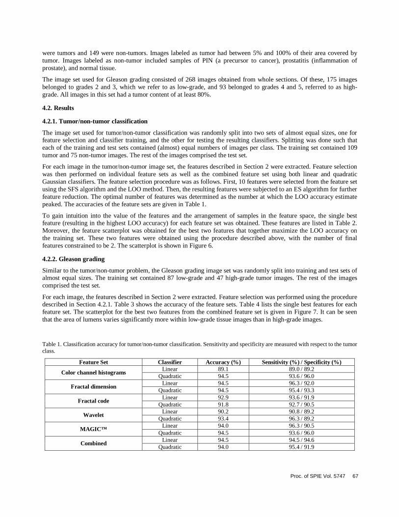
Table 1. Classification accuracy for tumor/non-tumor classification. Sensitivity and specificity are measured with respect to the tumor class.

Feature Set Classifier Accuracy (%) Sensitivity (%) / Specificity (%) Linear 89.1 89.0 / 89.2

Color channel histograms Quadratic 94.5 93.6 / 96.0

Linear 94.5 96.3 / 92.0 Fractal dimension

Quadratic 94.5 95.4 / 93.3 Linear 92.9 93.6 / 91.9

Fractal code Quadratic 91.8 92.7 / 90.5

Linear 90.2 90.8 / 89.2 Wavelet

Quadratic 93.4 96.3 / 89.2 Linear 94.0 96.3 / 90.5

MAGIC™ Quadratic 94.5 93.6 / 96.0

Linear 94.5 94.5 / 94.6 Combined

Quadratic 94.0 95.4 / 91.9

Proc. of SPIE Vol. 5747 67

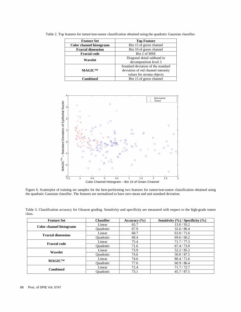
Table 2. Top features for tumor/non-tumor classification obtained using the quadratic Gaussian classifier.

Feature Set Top Feature Color channel histograms Bin 15 of green channel

Fractal dimension Bin 10 of green channel Fractal code Bin 2 of MSE

Wavelet Diagonal detail subband in

decomposition level 3

MAGIC™ Standard deviation of the standard deviation of red channel intensity

values for stroma objects Combined Bin 15 of green channel

Figure 6. Scatterplot of training set samples for the best-performing two features for tumor/non-tumor classification obtained using the quadratic Gaussian classifier. The features are normalized to have zero mean and unit standard deviation.

Table 3. Classification accuracy for Gleason grading. Sensitivity and specificity are measured with respect to the high-grade tumor class.

Feature Set Classifier Accuracy (%) Sensitivity (%) / Specificity (%) Linear 65.7 13.0 / 93.2

Color channel histograms Quadratic 67.9 32.6 / 86.4

Linear 68.7 63.0 / 71.6 Fractal dimension

Quadratic 68.4 69.6 / 60.2 Linear 75.4 71.7 / 77.3

Fractal code Quadratic 71.6 67.4 / 73.9

Linear 73.9 52.2 / 85.2 Wavelet

Quadratic 74.6 50.0 / 87.5 Linear 74.6 80.4 / 71.6

MAGIC™ Quadratic 77.6 60.9 / 86.4

Linear 72.4 71.7 / 72.7 Combined

Quadratic 73.1 45.7 / 87.5

-1.5 -1 -0.5 0 0.5 1 1.5 2 2.5 3 -3

-2

-1

0

1

2

3

4

Color Channel Histogram – Bin 15 of Green Channel

Non-tumor Tumor

MA

GIC

TM –

Sta

ndar

d D

evia

tion

of E

pith

elia

l Nuc

lei

Com

pact

ness

68 Proc. of SPIE Vol. 5747

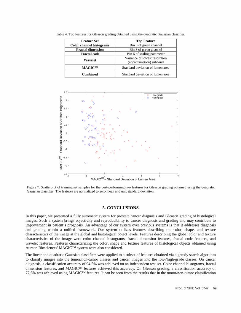
Table 4. Top features for Gleason grading obtained using the quadratic Gaussian classifier.

Feature Set Top Feature Color channel histograms Bin 8 of green channel

Fractal dimension Bin 3 of green ghannel Fractal code Bin 6 of scaling parameter

Wavelet Variance of lowest resolution

(approximation) subband

MAGIC™ Standard deviation of lumen area

Combined Standard deviation of lumen area

Figure 7. Scatterplot of training set samples for the best-performing two features for Gleason grading obtained using the quadratic Gaussian classifier. The features are normalized to zero mean and unit standard deviation.

5. CONCLUSIONS

In this paper, we presented a fully automatic system for prostate cancer diagnosis and Gleason grading of histological images. Such a system brings objectivity and reproducibility to cancer diagnosis and grading and may contribute to improvement in patient’s prognosis. An advantage of our system over previous systems is that it addresses diagnosis and grading within a unified framework. Our system utilizes features describing the color, shape, and texture characteristics of the image at the global and histological object levels. Features describing the global color and texture characteristics of the image were color channel histograms, fractal dimension features, fractal code features, and wavelet features. Features characterizing the color, shape and texture features of histological objects obtained using Aureon Biosciences' MAGIC™ system were also considered.

The linear and quadratic Gaussian classifiers were applied to a subset of features obtained via a greedy search algorithm to classify images into the tumor/non-tumor classes and cancer images into the low-/high-grade classes. On cancer diagnosis, a classification accuracy of 94.5% was achieved on an independent test set. Color channel histograms, fractal dimension features, and MAGIC™ features achieved this accuracy. On Gleason grading, a classification accuracy of 77.6% was achieved using MAGIC™ features. It can be seen from the results that in the tumor/non-tumor classification

-2 -1 0 1 2 3 4 -2.5

-2

-1.5

-1

-0.5

0

0.5

1

1.5

2

2.5

MAGICTM – Standard Deviation of Lumen Area

MA

GIC

TM –

Sta

ndar

d D

evia

tion

of A

rtifa

ct B

right

ness

Low-grade High-grade

Proc. of SPIE Vol. 5747 69

problem, simple features such as color channel histograms are able to achieve the same classification accuracy as complex features such as fractal dimension or the MAGIC™ features. For the problem of Gleason grading, however, the story is significantly different. The best classification accuracy in this case is obtained by the MAGIC™ features and using a quadratic classifier. This difference may be attributed to the difference in the complexity of the task. The tumor/non-tumor classification task must be significantly simpler than the problem of Gleason grading. In the latter case, finer differences in the structure of the tissue have to be taken into account. Our results show that MAGIC™ features may be capable of capturing the finer differences in tissue architecture that arises from different grades of tumor.

The MAGIC™ system is also part of a comprehensive prostate cancer recurrence prediction system using imaging, molecular, and clinical data11. Our results11 indicate that the image features provided by this system improve recurrence prediction over clinical and biochemical data.

REFERENCES

1. Cancer Facts & Figures. American Cancer Society, Inc., No. 5008.04, 2004. 2. J. Epstein, Prostate Biopsy Interpretation, 2nd ed. Lippincott-Raven, Philadelphia, PA, 1995. 3. D. F. Gleason, “The veteran's administration cooperative urologic research group: Histologic grading and clinical

staging of prostatic carcinoma,” in Urologic Pathology: The Prostate, M. Tannenbaum Ed. Lea and Febiger, Philadelphia, PA, 1977, pp. 171-198.

4. M. B. Amin, D. Grignon, P. A. Humphrey, and J. R. Srigley, Gleason Grading of Prostate Cancer: A Contemporary Approach. Lippincott Williams & Wilkins, New York, 2003.

5. J. Diamond, N. Anderson, P. Bartels, R. Montironi, and P. Hamilton, “The use of morphological characteristics and texture analysis in the identification of tissue composition in prostatic neoplasia,” Human Pathology, vol. 35, pp. 1121-1131, 2004.

6. M. A. Roula, J. Diamond, A. Bouridane, P. Miller, and A. Amira, “A multispectral computer vision system for automatic grading of prostatic neoplasia,” in Proc. Proc. IEEE Int. Symp. Biomed. Imaging, Washington, DC, 2002, pp. 193- 196.

7. R. Stotzka, R. Manner, P.H. Bartels, and D. Tompson, “A hybrid neural and statistical classifier system for histopathologic grading of prostate lesions,” Anal. Quant. Cytol. Histol., vol. 17, pp. 204-218, 1995.

8. Y. Smith, G. Zajieck, M. Werman, G. Pizov, and Y. Sherman, “Similarity measurement method for the classification of architecturally differentiated images,” Comp. Biomed. Res., vol. 32, pp. 1-12, 1999.

9. A. W. Wetzel, R. Crowley, S. J. Kim, R. Dawson, L. Zheng, Y. M. Joo, Y. Yagi, J. Gilbertson, C. Gadd, D. W. Deerfield and M. J. Becich, “Evaluation of prostate tumor grades by content-based image retrieval,” in Proc. SPIE AIPR Workshop on Advances in Computer-Assisted Recognition, vol. 3584, Washington, DC, 1999, pp. 244-252.

10. K. Jafari-Khouzani and H. Soltanian-Zadeh, “Multiwavelet grading of pathological images of prostate,” IEEE Trans. Biomed. Eng., vol. 50, pp. 697-704, 2003.

11. M. Teverovskiy, V. Kumar, J. Ma, A. Kotsianti, D. Verbel, A. Tabesh, H. Pang, Y. Vengrenyuk, S. Fogarasi, and O. Saidi, “Improved prediction of prostate cancer recurrence based on an automated tissue image analysis system,” in Proc. IEEE Int. Symp. Biomed. Imaging, Arlington, VA, 2004, pp. 257-260.

12. K. Fukunaga, Introduction to Statistical Pattern Recognition, 2nd ed. Academic, New York, 1990. 13. G. Landini “Applications of fractal geometry in pathology,” in Fractal Geometry in Biological Systems: An

Analytical Approach, P. M. Iannaccone and M. Khokha, Eds. CRC Press, Boca Raton, FL, 1996, pp.205-246. 14. N. Lu, Fractal Imaging. Academic, San Diego, CA, 1997. 15. A. E. Jacquin, “Fractal image coding: A review,” Proc. IEEE, vol. 81, pp. 1451-1465, 1993. 16. A. Laine and J. Fan, “Texture classification by wavelet packet signatures,” IEEE Trans. Pattern Anal. Machine

Intell., vol. 15, pp. 1186–1191, 1993. 17. I. Daubechies, Ten Lectures on Wavelets. SIAM, Philadelphia, PA, 1992. 18. R. C. Gonzales and R. E. Woods, Digital Image Processing. Addison-Wesley, New York, 1992. 19. M. Baatz and A. Schäpe, “Multiresolution segmentation: An optimization approach for high quality multi-scale

image segmentation,” in Angewandte Geographische Informationsverarbeitung XII, J. Strobl, T. Blaschke, and G. Griesebner, Eds. Wichmann-Verlag, Heidelberg, Germany, 2000, pp. 12-23.

20. R. O. Duda, R. E. Hart, and D. G. Stork, Pattern Classification, 2nd ed. Wiley, New York, 2001.

70 Proc. of SPIE Vol. 5747