Cell Cluster Graph for Prediction of Biochemical Recurrencein Prostate Cancer Patients from Tissue Microarrays

Sahirzeeshan Alia, Robert Veltrib, Jonathan A. Epsteinb, Christhunesa Christudassb andAnant Madabhushia

aDepartment of Biomedical Engineering, Case Western Univeristy, Cleveland, Ohio, USA;bDepartment of Surgical Pathology, The Johns Hopkins Hospital, Baltimore, Maryland, USA.

ABSTRACT

Prostate cancer (CaP) is evidenced by profound changes in the spatial distribution of cells. Spatial arrangementand architectural organization of nuclei, especially clustering of the cells, within CaP histopathology is knownto be predictive of disease aggressiveness and potentially patient outcome. Quantitative histomorphometry is arelatively new field which attempt to develop and apply novel advanced computerized image analysis and featureextraction methods for the quantitative characterization of tumor morphology on digitized pathology slides.Recently, graph theory has been used to characterize the spatial arrangement of these cells by constructinga graph with cell/nuclei as the node. One disadvantage of several extant graph based algorithms (Voronoi,Delaunay, Minimum Spanning Tree) is that they do not allow for extraction of local spatial attributes fromcomplex networks such as those that emerges from large histopathology images with potentially thousands ofnuclei. In this paper, we define a cluster of cells as a node and construct a novel graph called Cell Cluster Graph(CCG) to characterize local spatial architecture. CCG is constructed by first identifying the cell clusters to useas nodes for the construction of the graph. Pairwise spatial relationship between nodes is translated into edgesof the CCG, each of which are assigned certain probability, i.e. each edge between any pair of a nodes has acertain probability to exist. Spatial constraints are employed to deconstruct the entire graph into subgraphs andwe then extract global and local graph based features from the CCG. We evaluated the ability of the CCG topredict 5 year biochemical failures in men with CaP and who had previously undergone radical prostatectomy.Extracted features from CCG constructed using nuclei as nodal centers on tissue microarray (TMA) imagesobtained from the surgical specimens of 80 patients allowed us to train a support vector machine classifier via a3 fold randomized cross validation procedure which yielded a classification accuracy of 83.1± 1.2%. By contrastthe Voronoi, Delaunay, and Minimum spanning tree based graph classifiers yielded corresponding classificationaccuracies of 67.1± 1.8% and 60.7± 0.9% respectively.

1. PURPOSE

Graph theory has emerged as a method to characterize the structure of large complex networks leading to a betterunderstanding of dynamic interactions that exist between their components. Both local and global topographicalcharacteristics extracted from these graphs can define the network structure (topology) and relationships thatexist between different structures.1,2 Nodes with similar characteristics tend to cluster together and the patternof clustering provides information as to the shared group properties, and therefore the function of the individualnodes. In the context of image analysis and classification of digital pathology, some researchers have shown thatspatial graphs and tessellations such as those obtained via the Voronoi, Delaunay, and minimum spanning tree(MST), built using nuclei as vertices may actually have biological context and may thus be potentially predictiveof disease severity2,3 . These graphs have been mined for quantitative features that have shown to be usefulin the context of prostate and breast cancer grading.1,2 However, these topological approaches focus only onlocal-edge connectivity. Although Delaunay and its subgraph MST can be efficiently constructed in O(n log n)time, one of the computational bottlenecks is in the accurate identification of nuclear centroids (which is often

Further author information: (Send correspondence to Sahir Ali or Anant Madabhushi)Sahir Ali: E-mail: sna19@case.edu (or sahirali30@gmail.com), Telephone: (732)-6689586Anant Madabhushi: E-mail: axm788@case.edu, Telephone: (216) 368-8519

Medical Imaging 2013: Digital Pathology, edited by Metin N. Gurcan, Anant Madabhushi, Proc. of SPIE Vol. 8676, 86760H · © 2013 SPIE · CCC code: 1605-7422/13/$18

doi: 10.1117/12.2008695

Proc. of SPIE Vol. 8676 86760H-1

Downloaded From: http://proceedings.spiedigitallibrary.org/ on 05/08/2013 Terms of Use: http://spiedl.org/terms

difficult and time consuming) on large histopathology images. Moreover, these graphs inherently extract onlyglobal features and, therefore, important information at the local level may be left unexploited.

Prostate Cancer (CaP) is evidenced by profound histological, nuclear and glandular changes in the organi-zation of the prostate. Grading of surgically removed CaP is a fundamental determinant of disease biology andprognosis.4 The Gleason score, the most widespread method of prostate cancer tissue grading used today, is thesingle most important prognostic factor in CaP strongly influencing therapeutic options.4,7 The Gleason scoreis determined using the glandular and nuclear architecture and morphology within the tumor; the predominantpattern (primary) and the second most common pattern (secondary) are assigned numbers from 1-5. The sum ofthese 2 grades is referred to as the Gleason scores. Scoring based on the 2 most common patterns is an attemptto factor in the considerable heterogeneity within cases of CaP.4 In addition, this scoring method was found tobe superior for predicting disease outcomes compared with using the individual grades alone. Problems withmanual Gleason grading include inter-observer and intra-observer variation and these errors can lead to variableprognosis and suboptimal treatment.8

In recent years, computerized image analysis methods have been studied in an effort to overcome the sub-jectivity of the Gleason grading system.1,9, 10 An important prerequisite to such a computerized CaP gradingscheme, however, is the ability to accurately and efficiently segment histological structures (glands and nuclei)of interest. Perviously, texture based approaches in11,12 characterized tissue patch texture via wavlet featuresand fractal dimension. However, a limitation of these approaches were that the image patches were manuallyselected to obtain the region containing the tissue class on the digitized slide. Doyle, et al.2 showed that spatialgraphs (eg. Voronoi, Delaunay, minimum spanning tree) built using nuclei as vertices in digitized histopathologyimages, yielded a set of quantitative feature that allowed for improved separation between intermediate Glea-son patterns. Farjam, et al.14 employed gland morphology to identify the malignancy of biopsy tissues, whileDiamond et al.13 used morphological and texture features to identify 100-by-100 pixel tissue regions as eitherstroma, epithelium, or cancerous tissue (a three-class problem). Tabesh et al.3 developed a computer-aidedDiagnosis (CAD) system that employed texture, color, and morphometry on tissue microarrays to distinguishbetween cancer and non-cancer regions, as well as between high and low prostate cancer Gleason grades.

Biochemical recurrence (BcR) is a rise in the blood level of prostate-specific antigen (PSA) in CaP patientsafter treatment with surgery or radiation, and is often a marker for cancer recurrence.15 Biochemical recurrencefollowing radical prostatectomy is a relatively common finding, affecting approximately 25% of cases.15 Somestudies considered the percentage of high Gleason pattern as a factor predicting a higher rate of BcR.16 On theother hand, Chan et al. reported that high Gleason pattern is not likely to be reproducible.17 It was oftendifficult and time consuming and results in a prognostic effect only at its extremes (greater than 70% or lessthan 20% with pattern 4/5). Recently some researchers have suggested that tumor morphology alone might beable to tell us about disease aggressiveness to the same extent that molecular assays can.18 Consequently quan-titative histomorphometry or the use of advanced computerized image analysis and machine learning methodscould be used to predict disease aggressiveness and patient outcome based of standard haematoxylin and eosinstained pathology specimens alone. Veltri et al. showed that nuclear morphometric signatures can predict PSAreccurence in men with long-term follow post prostatectomy.8 In this paper we have developed novel quantitativehistomorphometric features (cell cluster graphs) that will allow us to go beyond predicting Gleason grade aloneand provides a direct way of predicting disease outcome in CaP.

The rest of this paper is organized as follows. In Section 2 we discuss our novel contributions and introduceCell Cluster Graphs in Section 3.

2. NOVEL CONTRIBUTIONS

This paper presents a novel computational model that relies solely on the organization of clusters of cancerouscells in a tumor. Despite their complex nature, cancerous cells tend to self-organize in clusters and exhibitarchitectural organization, an attribute which forms the basis of many cancers.4 In this paper, we present anovel cell cluster graph (CCG) that is computationally efficient and provides an effective tool to quantitativelycharacterize and represent tissue images according to the spatial distribution and clustering of cells. Traditionalgraphs (such as Voronoi, Delaunay and Minimum Spamming Trees) construct an overarching global graph with an

Proc. of SPIE Vol. 8676 86760H-2

Downloaded From: http://proceedings.spiedigitallibrary.org/ on 05/08/2013 Terms of Use: http://spiedl.org/terms

A,

intention of establishing connection between each and every node in a given graph. There are two disadvantagesof using these graphs:

1. Since these spatial graphs are globally constructed, we are limited to extracting only the global features(such as edge length statistics) while ignoring important local information (such as clustering and com-pactness of nodes). On the contrary, CCG is constructed locally by reducing the connections to distantnodes, resulting in disconnected subgraphs from which we can extract local features and information.

2. Cell graph implicitly provides separation of nuclei from epithelial regions from stromal regions. In thecontext of digital pathology, globally constructed spatial graphs establish connections between cells fromEpithelial and Stromal regions. This is an important consideration since the prognostic information istypically embedded within the tumor epithelium and the role of the stromal nuclei in disease aggressivenessis less clear. However, VT and DT graphs do not implicitly distinguish between stromal and epithelial nucleiand hence connected edges in these graphs traverse the stromal and epithelial regions (as seen in Figures1 (b), (c) and (f) ,(g)). This stromal-epithelial graph is probably less representative of tumor morphologycompared to a graph that specifically looks at spatial architecture and arrangement of epithelial nucleialone.

CCG (as described in Figure 2) is generated by nodes corresponding to nuclei clusters and the probabilityof a link between a pair of nodes is calculated as a decaying function of the Euclidean distance between thisnode pair. Since CCG defines a graph node as nuclear cluster rather than an individual nucleus, it does notrequire accurately resolving nuclei boundaries, and thus can be performed on low magnification images. Unlikecell graphs presented by Demir et al.,5 CCG does not depend on identifying accurate boundaries of nuclei. Weemployed watershed and concavity based technique to detect the approximate locations of the nuclei. A nucleicluster (which serves as a node) is identified by leveraging a technique based on concavity detection, whichidentifies overlapping and touching objects.6 We then extract subgraphs and use the topological features definedon each node of the subgraph, i.e., local graph metrics, to quantitatively characterize BcR in CaP patients. Inthis paper, we leverage CCG in conjunction with a machine learning algorithm to predict BcR in 80 patients.

(a) TMA - No BcR (b) Delaunay Graph (c) Voronoi Graph (d) CCG

(e) TMA - BcR (f) Delaunay Graph (g) Voronoi Graph (h) Cell Cluster GraphFigure 1. Examples of traditional graphs (Delaunay and Voronoi) and CCG being constructed on a TMA of tumor thatdid not undergo BcR (a,b, c, and d) and on a TMA of a tumor with BcR (e,f, g, and h).

Proc. of SPIE Vol. 8676 86760H-3

Downloaded From: http://proceedings.spiedigitallibrary.org/ on 05/08/2013 Terms of Use: http://spiedl.org/terms

Original Prostate TMA Nuclear cluster identification Cell Cluster Graph

0 No Recurrence + Recurrence

ClassificationFeature Extraction

Table 1. Description of notations and commonly used symbols in this paper.

Symbol Description Symbol Description

C 2D image scene x 2D Cartesian grid of pixels c = (x, y)

fg(c) function that assigns intensity values to pixel c s the shape contour

cw point on contour boundary Ω bounded open set in R2

F feature set Q selected subset of feature set

G = (V,E) graph - V (set of vertices) and E (set of edges) r distance threshold

α controls graph sparcity MI Mutual Information

u, v nodes (nuclei cluster) Uc centroids of clusters

3. CONSTRUCTING CLUSTER CELL GRAPHS

An image is defined as C = (x, fg) where x is a 2D grid representing pixels c ∈ x, with c = (x, y) representing theCartesian coordinates of a pixel and fg assigns intensity values to c ∈ x, where fg(c) ∈ R+ (gray scale). Formally,

Figure 2. Flow chart showing the various modules in construction of CCG. Step 1 is to apply watershed to get initialboundaries (left outer panel). Step 2 and 3 requires identifying clusters of nuclei and thereby identifying graph nodes asillustrated in the middle panel. Last step is to establish probablistic links (edges) between identified nodes (right panel).

CCG is defined by G = (V,E), where V and E are the set of nodes and the edges respectively. Construction ofCCG can be achieved in three steps as summarized below, graphically in Figure 2 and in Algorithm 1.

Quantization and Nuclear Detection The first step is to distinguish nuclei from the background. Weemploy the popular watershed transformation to obtain the initial delineations of nuclear boundaries in the entireimage and generating a binary mask from the result.

Proc. of SPIE Vol. 8676 86760H-4

Downloaded From: http://proceedings.spiedigitallibrary.org/ on 05/08/2013 Terms of Use: http://spiedl.org/terms

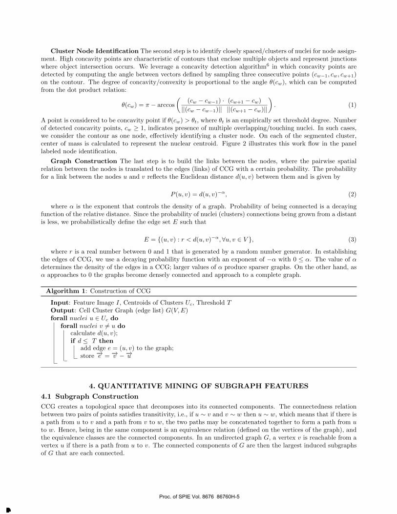
Cluster Node Identification The second step is to identify closely spaced/clusters of nuclei for node assign-ment. High concavity points are characteristic of contours that enclose multiple objects and represent junctionswhere object intersection occurs. We leverage a concavity detection algorithm6 in which concavity points aredetected by computing the angle between vectors defined by sampling three consecutive points (cw−1, cw, cw+1)on the contour. The degree of concavity/convexity is proportional to the angle θ(cw), which can be computedfrom the dot product relation:

θ(cw) = π − arccos

((cw − cw−1) · (cw+1 − cw)

||(cw − cw−1)|| ||(cw+1 − cw)||

). (1)

A point is considered to be concavity point if θ(cw) > θt, where θt is an empirically set threshold degree. Numberof detected concavity points, cw ≥ 1, indicates presence of multiple overlapping/touching nuclei. In such cases,we consider the contour as one node, effectively identifying a cluster node. On each of the segmented cluster,center of mass is calculated to represent the nuclear centroid. Figure 2 illustrates this work flow in the panellabeled node identification.

Graph Construction The last step is to build the links between the nodes, where the pairwise spatialrelation between the nodes is translated to the edges (links) of CCG with a certain probability. The probabilityfor a link between the nodes u and v reflects the Euclidean distance d(u, v) between them and is given by

P (u, v) = d(u, v)−α, (2)

where α is the exponent that controls the density of a graph. Probability of being connected is a decayingfunction of the relative distance. Since the probability of nuclei (clusters) connections being grown from a distantis less, we probabilistically define the edge set E such that

E = (u, v) : r < d(u, v)−α,∀u, v ∈ V , (3)

where r is a real number between 0 and 1 that is generated by a random number generator. In establishingthe edges of CCG, we use a decaying probability function with an exponent of −α with 0 ≤ α. The value of αdetermines the density of the edges in a CCG; larger values of α produce sparser graphs. On the other hand, asα approaches to 0 the graphs become densely connected and approach to a complete graph.

Algorithm 1: Construction of CCG

Input: Feature Image I, Centroids of Clusters Uc, Threshold TOutput: Cell Cluster Graph (edge list) G(V,E)forall nuclei u ∈ Uc do

forall nuclei v 6= u docalculate d(u, v);if d ≤ T then

add edge e = (u, v) to the graph;store −→e = −→v −−→u

4. QUANTITATIVE MINING OF SUBGRAPH FEATURES

4.1 Subgraph Construction

CCG creates a topological space that decomposes into its connected components. The connectedness relationbetween two pairs of points satisfies transitivity, i.e., if u ∼ v and v ∼ w then u ∼ w, which means that if there isa path from u to v and a path from v to w, the two paths may be concatenated together to form a path from uto w. Hence, being in the same component is an equivalence relation (defined on the vertices of the graph), andthe equivalence classes are the connected components. In an undirected graph G, a vertex v is reachable from avertex u if there is a path from u to v. The connected components of G are then the largest induced subgraphsof G that are each connected.

Proc. of SPIE Vol. 8676 86760H-5

Downloaded From: http://proceedings.spiedigitallibrary.org/ on 05/08/2013 Terms of Use: http://spiedl.org/terms

4.2 Extraction of Subgraph features

Unlike traditional graph based methods (VT and DT), we extract both global and local graph metrics (features)from the subgraphs or the entire graph, G. Table 2 summarizes the features we extract and their histologicalsignificance. Features referred to as ”Global” are those which are computed over the entire CCG and not overindividual sub-graphs.

Given a CCG, G(V,E) with N representing the set of nuclear cluster indices and E representing the set ofedges between the nodes, we extract following features from the CCG:

1. Average Eccentricity represents the eccentricity per node in the graph.∑Vu=1 εu|V |

(4)

where eccentricity of the uth node εu, u = 1 · |V |, is the maximum value of the shortest path length fromnode u to any other node in the graph.

2. Clustering Coefficient C is defined as the average of the local clustering coefficient Cu that representsthe ratio between the number of edges between the neighbors of a node u and the total possible number ofedges between the neighbors of node u.

C =

∑|V |u=1 Cu|V |

, (5)

Cu =|Eu|(ku2

) =2|Eu|

ku(ku − 1), (6)

where |Eu| is the number of edges between the nodes in the neighborhood of node u, ku is the number ofnodes in the neighborhood of node u.

3. Cluster Coefficient D is defined as the average of the local clustering coefficients Du that representsthe ratio between the number of edges between the neighbors of node u and the node u itself to the totalpossible number of edges between the neighbors of node u and the node u itself

D =

∑|V |u=1Du

|V |, (7)

Du =ku + |Eu|(

ku+12

) =2(ku + |Eu|)ku(ku + 1)

. (8)

4. Number of Connected Components represents the number of clusters in the graph (excluding theisolated points).

5. Giant Connected Component Ratio is the ratio between the number of the nodes in the largestconnected components in the graph and the number of nodes.

6. Number/Percentage of Isolated Nodes is the number/percentage of the nodes that have no incidentedges in the graph. Therefore, an isolated node has a degree of 0.

7. Skewness of Edge Length is one of the statistics of the edge length distribution in the graph.

Proc. of SPIE Vol. 8676 86760H-6

Downloaded From: http://proceedings.spiedigitallibrary.org/ on 05/08/2013 Terms of Use: http://spiedl.org/terms

CCG Feature Description Relevance to Histology

Clustering Coeff CRatio of total number of edges amongthe neighbors of the node to the totalnumber of edges that can exist amongthe neighbors of the node per node

Nuclei ClusteringClustering Coeff D

Ratio of total number of edges amongthe neighbors of the node and the nodeitself to the total number of edges thatcan exist among the neighbors of thenode and the node itself per node

Giant Connected ComponentRatio between the number of nodes inthe largest connected component in thegraph and total the number of nodes(Global)

# of Connected ComponentsNumber of clusters in the graph exclud-ing the isolated nodes (Global)

Average EccentricityAverage of node eccentricities where theeccentricity of a node is the maximumshortest path length from the node toany other node in the graph

Compactness of Nuclei

Percentage of Isolated PointsPercentage of the isolated nodes in thegraph, where an isolated node has a de-gree of 0

Number of Central PointsNumber of nodes within the graphwhose eccentricity is equal to the graphradius

Skewness of Edge Lengths Statistics of the edge length distribu-tion in the graph

Spatial Uniformity

Table 2. Description of the features extracted from CCG .

Feature Class Extracted Features Relevance to Histology

Voronoi TesselationArea Standard Deviation, Area Average, Area Min-imum / Maximum Area Disorder, Perimeter Stan-dard Deviation, Perimeter Average, Perimeter Min-imum / Maximum, Perimeter Disorder

Tissue Architecture

Delaunay TriangulationSide Length Standard Deviation, Side Length Dis-order, Triangle Area Minimum / Maximum, Trian-gle Area Standard Deviation, Triangle Area Average,Triangle Area Disorder

Table 3. Summary features derived from traditional graphs (Voronoi and Delaunay) constructed on CaP TMA with nucleias centroids.

5. MINIMUM REDUNDANCY MAXIMUM RELEVANCE FEATURE SELECTIONSCHEME

We utilize the minimum Redundancy Maximum Relevance (mRMR) feature selection scheme19 in order toidentify an ensemble of features that will allow for optimal classification of BcR vs No BcR in CaP. The featureselection scheme is used to identify the most discriminatory attributes from among all of the CCG featuresextracted.

In the following description, the selected subset of features Q is comprised of feature vectors Fi, i ∈ 1, ..., |Q|(note that F = F1, ..., FN, Q ⊂ F and |Q| < N). The mRMR scheme attempts to simultaneously optimize

Proc. of SPIE Vol. 8676 86760H-7

Downloaded From: http://proceedings.spiedigitallibrary.org/ on 05/08/2013 Terms of Use: http://spiedl.org/terms

two distinct criteria. The first is ”maximum relevance” which selects features Fi that have the maximal mutualinformation (MI) with respect to the corresponding label vector L. This is expressed as

U =1

|Q|∑Fi∈Q

MI(Fi, L) (9)

The second is ”minimum redundancy” which ensures that selected features Fi, Fj ∈ Q, i, j ∈ 1, ..., |Q|, arethose which have the minimum MI with respect to each other, given as

V =1

|Q|2∑

Fi,Fj∈Q

MI(Fi, Fj) (10)

Under the second constraint, the selected features will be maximally dissimilar with respect to each other,while under the first, the feature selection will be directed by the similarity with respect to the class labels. Thereare two major variants of the mRMR scheme: the MI difference (MID, given by U − V ) and the MI quotient(MIQ, given by U/V ). These variants represent different techniques to optimize the conditions associated withmRMR feature selection. In this study, we evaluated the use of both MID and MIQ for feature selection as wellas determined an optimal number of features by varying |Q| the mRMR algorithm.

6. EXPERIMENTAL DESIGN AND RESULTS

6.1 Data Description

Our Prostate dataset comprised a total of 80 patient studies with CaP in the form of tissue microarrays (TMA)with 4 TMAs per patient study. The various CaP tissues and controls included in these TMAs were selected andreviewed by a pathologist at Johns Hopkins University Hospital. Slides from all cases selected are reviewed bya pathologist and the normal-appearing and staged and/or graded index tumor areas are identified and markedon the slide for each case. Using these template slides marked for normal-appearing (adjacent) and diagnosticCaP areas, the tissue blocks are marked using the template slides, and 0.60mm cores are punched from thenormal-appearing and CaP areas and then transferred to recipient blocks. The TMAs are prepared (bothnormal-appearing and cancer areas) using a Beecher MT1 manual arrayer (Beecher Instruments, Silver Spring,MD) in the Johns Hopkins Hospital TMAJ pathology core facility. Each TMA is constructed using four replicate0.6mm core tissue samples from the normal-appearing and cancer areas of each patient who had undergone radicalprostatectomy for CaP. The dataset contains 10 years survival outcome data which also contains 10 year BcRdata following prostate surgery. Out of 80 patients, BcR occurred in 20 patients (25%) (summarized in Table 4).

6.2 Qualitative Evaluation of CCG

Figure 1 illustrates DT, VT and CCG graphs constructed on two CaP TMAs (with BcR and no BcR). The CCGgraph is able to constructed on a significantly down-sampled version image compared to VT and DT. Unlike DTand VT, CCG breaks the overall graph structure into various disconnected graphs, hence enabling extraction oflocal features. Cell graph implicitly provides separation of nuclei from epithelial regions from stromal regions.This is an important consideration since the prognostic information is typically embedded within the tumorepithelium and the role of the stromal nuclei in disease aggressiveness is less clear. However the VT and DTgraphs do not implicitly distinguish between stromal and epithelial nuclei and hence the connected edges in thesegraphs traverse the stromal and epithelial regions (shown in Figure 1). This stromal-epithelial graph is probablyless representative of tumor morphology compared to a graph that specifically looks at spatial architecture andarrangement of epithelial nuclei alone. While explicitly separating stroma and epithelium is an option, in spiteof the presence of automated computerized segmentation algorithms purporting to do this accurately,20 this stillremains a very difficult problem. The CCG offers an alternative to explicit segmentation of stromal and epithelialregions in that it implicitly forms subgraphs within the epithelial regions and given the sparsity of nuclei in thestromal areas, results in no stromal CCGs (Figure 2). As CCG is constructed locally with probabilistic edgeconnections that are encoded via a distance function, epithelial to stromal traversal is removed, as illustrated inFigures 2(g) and 2(h).

Proc. of SPIE Vol. 8676 86760H-8

Downloaded From: http://proceedings.spiedigitallibrary.org/ on 05/08/2013 Terms of Use: http://spiedl.org/terms

Follow-up Category Measure # of Samples # of patients had BcR(PSA >= 0.2 ng/ml)

No recurrence PSA < 0.2 49 0

Increase in PSA PSA 0.2 or greater 12 12

Local recurrence ofPCa

1 1

Distant metastasis 2 2

Both local recur-rence and distantmetastasis

2 2

Decrease in PSAthrough RadiationTreatment

PSA becomes < 0.2 after Rx 3 3

Died from any non-prostate cancer re-lated cause

1 0

No follow-up data 10 –

Table 4. Detailed description of the patient data associated with biochemical recurrence used in this study.

6.3 Classifier Training and Evaluation

To evaluate the performance of the CCG features in distinguishing between patients with and without BcR basedoff a histomorphometric analysis of the digitized TMA specimens alone, we trained a Support vector machineclassifier with a subset of features in Table 2 and identified as being relevant by the feature selection scheme. Inaddition, we compared the performance of graph based attributes (Table 3) obtained by constructing VT andDT graphs by using all the nuclei identified by the watershed algorithm in the image.

We compared the performance of the classifiers in predicting 10 year BcR in the 80 patient cohort (see Table4) between the CCG, VT, and DT based graphs. Table 5 shows most significant CCG features identified bymRMR over the entire set of CCG features extracted and illustrated in Table 2. The Clustering and compactnessfeatures were identified by the mRMR algorithm in distinguishing tumors that will undergo BcR from the onesthat will not. Table 2 attempts to provide some insight into why these features were found to be so discriminatory.Furthermore, samples with discrete clusters of nuclei have a low percentage of central points while uniformlydistributed cells (non-clustering) have a high percentage of central points.

We achieved an accuracy of 83.1± 1.2% in predicting biochemical failure against Voronoi Diagram (VD) andDelauny Triangulation (DT) using a randomized 10 runs of 3 fold cross-validation procedure. SVM classifier wastrained on a linear kernel.

7. CONCLUDING REMARKS

In this work, we presented a novel Cell Cluster Graph (CCG) that solely relies on the arrangement of clusteringnuclei. CCG graphs provide sparse representation for quantification tumor morphology and nuclear architecturein large tissue images that contain thousands of nuclei. Unlike traditional graph based approaches (Voronoiand Delauny), CCG analyzes clusters of cells which takes away the daunting task of segmenting individualcells, a computational heavy and a challenging task. Moreover, CCG implicitly distinguishes between stromaland epithelial nuclei and hence enables us to focus on the prognostic information embedded within the tumorepithelium. CCG derived features from prostate cancer (CaP) TMAs were evaluated via SVM classifier ability toidentify CaP patients at risk for 10 year biochemical failure post-surgery. to predict biochemical failures in CaP.CCG predicted biochemical failure in CaP patients with 83.1% accuracy, yielding significantly improved resultsover traditional graph-based methods. For future studies, we will extend this methodology to other cancers todevelop prognostic image based markers for predicting patient outcome.

Proc. of SPIE Vol. 8676 86760H-9

Downloaded From: http://proceedings.spiedigitallibrary.org/ on 05/08/2013 Terms of Use: http://spiedl.org/terms

.A

Feature Class Histological Significance

Clustering Coeff C & D

(a) High Nuclei Density (b) Low Nuclei DensityHigher Clustering Coefficient Lower Clustering Coefficient

Number of Central Points

(c) Uniform Clusters (d) Discrete ClustersHigh percentage of central points Low percentage of central points

Table 5. Description of the most significant CCG features identified by the mRMR scheme and an illustration of whythe features identified (clustering coefficient and number of central points) are able to discriminate between the BcR(represented by patches a and d) and non-BcR (represented by patches b and c) cases.

Voronoi Delaunay CCG67.1± 1.8% 60.7± 0.9% 83.1± 1.2%

Table 6. Comparison of CCG against other graph based methods in predicting biochemical failure. SVM based classifierwas trained on features extracted from the graphs with 10 runs of 3-fold cross validation.

Acknowledgements

This work was made possible by grants from the National Institute of Health (R01CA136535, R01CA140772,R43EB015199, R21CA167811), National Science Foundation (IIP-1248316), and the QED award from the Uni-versity City Science Center and Rutgers University.

REFERENCES

1. A. Madabhushi, Digital Pathology Image Analysis: Opportunities and Challenges (Editorial), Imaging inMedicine, vol. 1(1), pp. 7-10, 2009.

2. S. Doyle, M. Hwang, K. Shah, A. Madabhushi, J. Tomasezweski and M. Feldman, ”Automated Grading ofProstate Cancer using Architectural and Textural Image Features”, ISBI, pp. 1284-87, 2007.

3. Tabesh, A., Teverovskiy, M., Pang, H., Verbel, V. K. D., Kotsianti, A., Saidi, O., 2007. ”Multifeature prostatecancer diagnosis and gleason grading of histological images.” IEEE Trans on Med. Imaging 26 (10), 13661378.

4. Epstein, J., Allsbrook, W., Amin, M., Egevad, L., ”The 2005 international society of urological pathology(isup) consensus conference on gleason grading of prostatic carcinoma,” American J. of Surgical Pathology29 (9), 12281242. 2005.

Proc. of SPIE Vol. 8676 86760H-10

Downloaded From: http://proceedings.spiedigitallibrary.org/ on 05/08/2013 Terms of Use: http://spiedl.org/terms

5. Demir, C and Gultekin, S.H . ”Augmented Cell-graphs for Automated Cancer Diagnosis.” BioinformaticsVol. 21 Suppl. 2 2005 pp 7–12.

6. Fatakdawala, H, Xu, J, Basavanhally, A, Bhanot, G, Ganesan, S, Feldman, M, Tomaszewski, J, Madabhushi,A, ”Expectation Maximization driven Geodesic Active Contour with Overlap Resolution (EMaGACOR):Application to Lymphocyte Segmentation on Breast Cancer Histopathology,” IEEE TBME, vol.57(7), pp.1676-1689, 2010.

7. Epstein, J., Walsh, P., Sanfilippo, F., ”Clinical and cost impact of second-opinion pathology. review ofprostate biopsies prior to radical prostatectomy.” American Journal of Surgical Pathology 20 (7), 851857.1996.

8. R.W. Veltri, S. Isharwal, M. C. Mille, ”Nuclear Roundness Variance Predicts Prostate Cancer Progres-sion,Metastasis, and Death: A Prospective EvaluationWith up to 25 Years of Follow-Up After RadicalProstatectomy”, The Prostate., vol. 70, 133m-1339, 2010.

9. Hipp, J., Flotte, T., Monaco, J., Cheng, J., Madabhushi, A., Yagi, Y., Rodriguez-Canales, J., Emmert-Buck,M., Dugan, M., Hewitt, S., Toner, M., Tompkins, R., Lucas, D., Gilbertson, J., Balis, U., 2011. ”Computeraided diagnostic tools aim to empower rather than replace pathologists: Lessons learned from computationalchess.” Journal of Pathology Informatics 2 (1), 25.

10. M. Gurcan, L. Boucheron, A. Can, A. Madabhushi, N. Rajpoot, B. Yener, Histopathological Image Analysis:A Review, IEEE Reviews in Biomedical Engineering, vol. 2, pp. 147-171, 2009.

11. K. Jafari-Khouzani, H. Soltanian-Zadeh, ”Multiwavelet grading of pathological images of prostate”, Biomed-ical Engineering, IEEE Transactions on 50 (2003) 697 704.

12. P.-W. Huang, C.-H. Lee, ”Automatic Classification for Pathological. Prostate Images Based on FractalAnalysis,” Medical Imaging, IEEE Transactions on 28 (2009) 1037 1050.

13. Diamond, J., Anderson, N., Bartels, P., Montironi, R., Hamilton, P., 2004. The use of morphological char-acteristics and texture analysis in the identification of tissue composition in prostatic neoplasia. HumanPathology35 (9), 11211131.

14. Farjam, R., Soltanian-Zadeh, H., Jafari-Khouzani, K., Zoroofi, R., 2007. ”An image analysis approach for au-tomatic malignancy determination of prostate pathological images”. Cytometry Part B (Clinical Cytometry)72 (B), 227240.

15. Ahmed F. Kotb and Ahmed A. Elabbady, Prognostic Factors for the Development of Biochemical Re-currence after Radical Prostatectomy, Prostate Cancer, vol. 2011, Article ID 485189, 6 pages, 2011.doi:10.1155/2011/485189

16. M. Noguchi, T. A. Stamey, J. E. McNeal, and C. M. Yemoto, ”Preoperative serum prostate specific antigendoes not reflect biochemical failure rates after radical prostatectomy in men with large volume cancers,”Journal of Urology, vol. 164, no. 5, pp. 15961600, 2000.

17. T. Y. Chan, A. W. Partin, P. C. Walsh, and J. I. Epstein, ”Prognostic significance of Gleason score 3+4versus Gleason score 4+3 tumor at radical prostatectomy, Urology, vol. 56, no. 5, pp. 823827, 2000.

18. Britta Weiglet and Jorge S Reis-Filho, ”Molecular profiling offers no more than tumor morphology and basicimmunohistochemistry”, Breast Cancer Research, 12:24. 2010.

19. Peng H, Long F, Ding C. ”Feature selection based on mutual information criteria of max-dependency,max-relevance, and min-redundancy”. Pattern Analysis and Machine Intelligence, IEEE Transactions on2005;27:1226-1238.

20. Andrew Janowczyk, Sharat Chandran, Anant Madabhushi, ”Quantifying local heterogeneity via morphologicscale: Distinguishing tumoral from stromal regions”, Journal of Pathology Informatics 2013

Proc. of SPIE Vol. 8676 86760H-11

Downloaded From: http://proceedings.spiedigitallibrary.org/ on 05/08/2013 Terms of Use: http://spiedl.org/terms