Automated diagnosis of Lungs Tumor Using Segmentation ...
227
www.ijecs.in International Journal Of Engineering And Computer Science ISSN: 2319-7242 Volume 5 Issue 10 Oct. 2016, Page No. 18350-18357 S.Piramu Kailasam 1 IJECS Volume 05 Issue 10 Oct., 2016 Page No.18350-18357 Page 18350 Automated diagnosis of Lungs Tumor Using Segmentation Techniques S.Piramu Kailasam 1 ,Dr. M. Mohammed Sathik 2 1 Research and Development Centre,Bharathiar University,India E-mail:[email protected] 2 Principal, Sathakathullah Appa College, India E-mail:[email protected] Abstract— The Objective is to detect the cancerous lung nodules from 3D CT chest image and classify the lung disease and its severity. Although so many researches has been done in this stream, the problem still remains a challenging one. To extract the lung region FCM segmentation is used. Here we used six feature extraction techniques such as bag of visual words based on the histogram oriented gradients, the wavelet transform based features, the local binary pattern, SIFT and Zernike moment . The Particle swarm optimization algorithm is used to select the best features. Keywords— Lungs CT, image segmentation, PSO, SVM, ELM, k- NN, NB. I. INTRODUCTION Due to increasing rate of smoking and air pollution lung cancer is main cause for deaths in different countries. CT is the best modality to diagnose the lung disease. Time and cost are the two important factors. The early detection of lung nodule growth cure the disease of the patient. According to staging of lung cancer the severity will be found. The radiologist will help the diagnosis efficiency by calculating the number of nodule growth in stages X rays image is not sufficient for early detection of lung cancer [2], [4]. CT plays an important role on cancer staging evaluation. It is challenging task due to low contrast, size and location variation in CT imaging. Distinguishing the cancerous nodules from the blood vessel is the challenging task because in the central lung regions lung nodules are confused with the blood vessels imaged in cross section. The detection of lung nodule have been found such as feature base, template matching based and neural based. In [5] the organs of interest and lung area was classified in to two clusters, air cluster and other organs cluster. Using Gaussian distribution as reference images, template matching algorithm is used to detect the nodules in chest CT images. Tuo Xu et al.[1] proposed an automatic global edge and region force (ERF) field guided method for lung field segmentation. Experimental results demonstrated that the proposed method is time efficient and improves the accuracy, sensitivity, specificity and robustness of the segmentation results. In the lungs accurate lung segmentation allows the detection and quantification of abnormalities. A automatic method for segmentation of the lungs and lobes from thorox CT scans by Van Rikrort et al. [7]. Here region growing approach is used to segment the region and morphological operations are done. Multiatlas segmentation will be applied to the results. Sobel edge [9] detection method is used to segment the CT lung image. Jun lai et al.[8] used a fully automatic segmentation for pulmonary vessals in plain thoraic CT images. Vessal tree reconstruction algorithm [10] reduced the number of false positives by 38%. Camarlinght et al.[11] has used three different computer aided detection techniques to identify the pulmonary nodules in CT images. Abdulla & Shaharun [12] used feed forward neural networks to classify lung nodules in X-ray images and with smaller feature of area, size and perimeter. Kuruvilla et al.[13] have used six distint parameters including skewness and fifth and sixth central moments extracted from segmented single slices and used feed forward back propagation neural network with them to evaluate accuracy . In Riccardi et al[16] the authors presented a new algorithm to automatically detect nodules with 71% overall accuracy using 3D radical transforms . In neuro imaging data of brain using deep Boltzmann machine for AD/MDC diagnosis is done by the author Suk et al. [17]. The method achieves a excellent diagnostic accuracy of 95.52%.To the best of our knowledge there has been no work that uses deep features from lung nodule classification. In this paper the trainned image was preprocessed then the lung region will be extracted using FCM segmentation. After that we found the lung cancer detection by extracting the features. Cancerous lung nodules detection from CT chest image The block diagram of the proposed method is shown in fig.1. To detect the location of the cancerous lung nodules this paper uses a novel algorithm. First we denoised the input image by wiener filter. Contrast is enhanced by histogram equalization. To extract the lung region the FCM segmentation is used. The further details of these are discussed below:
-
Upload
khangminh22 -
Category
Documents
-
view
1 -
download
0
Transcript of Automated diagnosis of Lungs Tumor Using Segmentation ...

www.ijecs.in
International Journal Of Engineering And Computer Science ISSN: 2319-7242
Volume 5 Issue 10 Oct. 2016, Page No. 18350-18357
S.Piramu Kailasam1 IJECS Volume 05 Issue 10 Oct., 2016 Page No.18350-18357 Page 18350
Automated diagnosis of Lungs Tumor Using Segmentation Techniques S.Piramu Kailasam
1,Dr. M. Mohammed Sathik
2
1 Research and Development Centre,Bharathiar University,India
E-mail:[email protected] 2Principal, Sathakathullah Appa College, India
E-mail:[email protected]
Abstract— The Objective is to detect the cancerous lung nodules from 3D CT chest image and classify the lung disease and its severity.
Although so many researches has been done in this stream, the problem still remains a challenging one. To extract the lung region FCM
segmentation is used. Here we used six feature extraction techniques such as bag of visual words based on the histogram oriented gradients,
the wavelet transform based features, the local binary pattern, SIFT and Zernike moment . The Particle swarm optimization algorithm is
used to select the best features.
Keywords— Lungs CT, image segmentation, PSO, SVM, ELM, k-
NN, NB.
I. INTRODUCTION
Due to increasing rate of smoking and air pollution lung
cancer is main cause for deaths in different countries. CT is the
best modality to diagnose the lung disease. Time and cost are
the two important factors. The early detection of lung nodule
growth cure the disease of the patient. According to staging
of lung cancer the severity will be found. The radiologist will
help the diagnosis efficiency by calculating the number of
nodule growth in stages X rays image is not sufficient for
early detection of lung cancer [2], [4]. CT plays an important
role on cancer staging evaluation. It is challenging task due to
low contrast, size and location variation in CT imaging.
Distinguishing the cancerous nodules from the blood vessel is
the challenging task because in the central lung regions lung
nodules are confused with the blood vessels imaged in cross
section. The detection of lung nodule have been found
such as feature base, template matching based and neural
based. In [5] the organs of interest and lung area was
classified in to two clusters, air cluster and other organs
cluster. Using Gaussian distribution as reference images,
template
matching algorithm is used to detect the nodules in chest CT
images. Tuo Xu et al.[1] proposed an automatic global edge
and
region force (ERF) field guided method for lung field
segmentation. Experimental results demonstrated that the
proposed method is time efficient and improves the accuracy,
sensitivity, specificity and robustness of the segmentation
results. In the lungs accurate lung segmentation allows the
detection and quantification of abnormalities. A automatic
method for segmentation of the lungs and lobes from thorox
CT scans by Van Rikrort et al. [7]. Here region growing
approach is used to segment the region and morphological
operations are done. Multiatlas segmentation will be applied to
the results. Sobel edge [9] detection method is used to segment
the CT lung image. Jun lai et al.[8] used a fully automatic
segmentation for pulmonary vessals in plain thoraic CT
images.
Vessal tree reconstruction algorithm [10] reduced the
number of false positives by 38%. Camarlinght et al.[11] has
used three
different computer aided detection techniques to identify the
pulmonary nodules in CT images.
Abdulla & Shaharun [12] used feed forward neural
networks to classify lung nodules in X-ray images and with
smaller feature of area, size and perimeter. Kuruvilla et al.[13]
have used six distint parameters including skewness and fifth
and sixth central moments extracted from segmented single
slices and used feed forward back propagation neural network
with them to evaluate accuracy . In Riccardi et al[16] the
authors presented a new algorithm to automatically detect
nodules with 71% overall accuracy using 3D radical
transforms . In neuro imaging data of brain using deep
Boltzmann machine for AD/MDC diagnosis is done by the
author Suk et al. [17]. The method achieves a excellent
diagnostic accuracy of 95.52%.To the best of our knowledge
there has been no work that uses deep features from lung
nodule classification. In this paper the trainned image was preprocessed then
the lung region will be extracted using FCM segmentation.
After that we found the lung cancer detection by extracting the
features.
Cancerous lung nodules detection from CT chest
image
The block diagram of the proposed method is shown in
fig.1. To detect the location of the cancerous lung nodules this
paper uses a novel algorithm. First we denoised the input
image by wiener filter. Contrast is enhanced by histogram
equalization. To extract the lung region the FCM segmentation is used. The further details of these
are discussed below:

DOI: 10.18535/ijecs/v5i10.22
S.Piramu Kailasam1 IJECS Volume 05 Issue 10 Oct., 2016 Page No.18350-18357 Page 18351
Fig.1 Cancerous lung nodule detection
A. GETTING THE ORIGINAL IMAGE
In this module, this paper get the original image for
the segmentation of the lung from the CT image.
B. PREPROCESSING
In an easy way making the image ready for the
processing is known as Preprocessing. Preprocessing is an
improvement of the image data that suppresses unwanted
degraded pixels important for futher processing.
I. Apply Denoising using Wiener Filter
In signal processing, the Wiener filter is a filter used
to produce an estimate of a desired or target random process
by linear time-invariant filtering an observed noisy process,
assuming known stationary signal and noise spectra, and
additive noise. The Wiener filter minimizes the mean square
error between the estimated random process and the desired
process. The goal of the Wiener filter is to filter out noise that
has corrupted a signal. It is based on a statistical approach, and
a more statistical account of the theory is given in the MMSE
estimator article. Typical filters are designed for a
desired frequency response. However, the design of the
Wiener filter takes a different approach. One is assumed to
have knowledge of the spectral properties of the original signal
and the noise, and one seeks the linear time-invariant filter
whose output would come as close to the original signal as
possible. Wiener filters are characterized by the following:
1. Assumption: signal and (additive) noise are stationary
linear stochastic processes with known spectral
characteristics or known autocorrelation and cross-
correlation
2. Requirement: the filter must be physically
realizable/causal (this requirement can be dropped,
resulting in a non-causal solution)
3. Performance criterion: minimum mean-square
error (MMSE)
II. Apply Contrast Enhancement
Digital image processing is still new enough for most
people that no matter how much this paper read, experiment
and work at it, there seems to be an endless amount to learn.
This is particularly true as regards photoshop that invaluable
tool yet also bottomless pit of a time sink. But every now and
then a little tidbit comes along that moves ones work either
easier or better, and this one, which I call Contrast
Enhancement – is one of the best that I have seen in a while.
The imadjust increases the contrast of the image by
mapping the values of the input intensity image to new values
such that, by default, 1% of the data is saturated at low and
high intensities of the input data.
C. LUNG REGION EXTRACTION
I. Apply FCM Segmentation
In fuzzy clustering, every point has a degree of belonging
to clusters, as in fuzzy logic, rather than belonging completely
too just one cluster. Thus, points on the edge of a cluster may
be in the cluster to a lesser degree than points in the center of
cluster. An overview and comparison of different fuzzy
clustering algorithms is available. Any point x has a set of
coefficients giving the degree of being in the kth cluster wk(x).
With fuzzy c-means, the centroid of a cluster is the mean of all
points, weighted by their degree of belonging to the cluster:
The degree of belonging, wk(x), is related inversely to the
distance from x to the cluster center as calculated on the
previous pass. It also depends on a parameter m that controls
how much weight is given to the closest center. The fuzzy c-
means algorithm is very similar to the k-means algorithm:
Choose number of clusters.
Assign randomly to each point coefficients for being
in the clusters.
Repeat until the algorithm has converged (that is, the
coefficients change between two iterations is no
more than , the given sensitivity threshold) :
a)Compute the centroid for each cluster, using
the formula above.
b)For each point, compute its coefficients of
being in the clusters, using the formula above.
II. Extraction of Lung Region
In this technique, the lung region is obtained by the
extraction method. The input is from the segmented region and
it extracts the lung region and gives the output image.
D. SEGMENTING THE LUNG REGION I. Applying Filling Holes
In this method, after extracting the lung region the holes in
the lung region are filled by the segmentation techniques.
E. LUNG CANCER DETECTION I. Extract Features
Feature extraction involves simplifying the amount of
resources required to describe a large set of data accurately.
Usually, one of the main problems in analyzing complex data
is the large number of variables involved in the data. A lot of
memory and computation power is necessary to analyze the
data . But feature extraction method can be used to
construction of variable combinations to overcome these
obstacles but it still describes data accurately. So achievement

DOI: 10.18535/ijecs/v5i10.22
S.Piramu Kailasam1 IJECS Volume 05 Issue 10 Oct., 2016 Page No.18350-18357 Page 18352
of best result happens. when an expert constructs a set of
application-dependent features.
II. Detect the Lung Cancer
After the extraction of the features from the image, by
using the features the cancer in the lungs was identified.
F. LOCALIZE THE LUNG CANCER
In computer vision and image processing, this paper often
perform different processing on ―objects‖ than on ―texture.‖ In
order to do this, this paper must have a way of localizing
textured regions of an image. For this purpose, this paper
suggest a working definition of texture: Statistics describes the
term ―texture‖ more accurately when compared to describing
the configuration of all the parts. Texture is a part of local
statistics. But Outliers do not seen to be local statistics and
draw our attention. This definition suggests that to find texture
this paper first extract certain basic features and compute their
local statistics. Then this paper compute a measure of saliency,
or degree to which each portion of the image seems to be an
outlier to the local feature distribution, and label as texture the
regions with low saliency. This paper present a method, based
upon this idea, for labeling points in cancer images as
belonging to texture regions. This method is based upon recent
psychophysics results on processing of texture.
I. Lung tissue classification and severity finding
The overall block diagram of the proposed method is
shown in Fig. 3.1. After finding the location of the cancerous
lung nodules the next process is to classify the lung disease
name and its severity based on the feature extraction. Among
several feature extraction methods this paper uses six feature
extraction technique such as the bag of visual-words based on
the histogram of oriented gradients, the wavelet transform-
based features, the local binary pattern, SIFT, Zernike
Moment. After extracting the features the Particle Swarm
Optimization (PSO) algorithm is used for select the best
features. Finally these features are classified by using the
Extreme Learning Machine (ELM) method. To analyse the
performance of the ELM method it is compared with the five
commonly used classifiers including support vector machine
(SVM), Bagging (Bag), Naive Bayes (NB), k-nearest neighbor
(k-NN), Extreme Learning Machine (ELM) and AdaBoost
(Ada).
II.Methods
The features are extracted from the Lungs CT dataset.
This project extracts four types of ROI features, including the
bag-of-visual-words based on the HOG (B-HOG), the wavelet
features, the LBP, and the CVH. We have 18-D B-HOG
features, 26-D wavelet features, 96-D LBP features, and 40-D
CVH features. Total 180 features are extracted. The details of
each type of features are given as follows.
I. B-HOG:
The HOG feature is a texture descriptor describing the
distribution of image gradients in different orientations.
Following the HOG feature extraction scheme of Dalal and
Triggs, we divide a ROI into smaller rectangular blocks of 8 ×
8 pixels and further divide each block into four cells of 4 × 4
pixels. An orientation histogram which contains nine bins
covering a gradient orientation range of 0–180° is computed
for each cell. Then, a block is represented by the linking of the
orientation histograms of cells in it. This means a 36-D HOG
feature vector is extracted for each block.
The commonly used image representation based on HOG
features is to join the feature vectors of all the blocks in the
image in sequence.All the HOG based images should have the
same size. Because , in the absence of same sized image
diverse resultant feature vector are obtained. But in CT lung
images, the size of ROIs differ patient to patient and different
lesions of the lungs. So the HOG based image has the obstacle
which makes it non applicable in this study. To solve this
problem, we adopt the bag-of-visual-words on HOG features
as the ROI representation. However, different from the
original bag-of-visual-words method, we use a clustering
algorithm based on Gaussian mixture modeling (GMM),
instead of the k-means algorithm, to generate more accurate
visual words. In this paper, total 18 visual words are obtained.
The 36-D HOG feature vector of each block is mapped to
the visual word corresponding to the highest likelihood for it.
Then, the number of HOG feature vectors assigned to each
visual word is accumulated and normalized by the number of
all the HOG feature vectors to form a 18-D histogram
representation of the ROI.
II. WAVELET FEATURES:
Wavelets are important and commonly used feature
descriptors for texture analysis, due to their effectiveness in
capturing localized spatial and frequency information and
multiresolution characteristics. In this paper, the ROIs are
decomposed to four levels by using 2-D symlets wavelet
because the symlets wavelet has better symmetry than
Daubechies wavelet and more suitable for image processing.
Then, the horizontal, vertical, and diagonal detail coefficients
are extracted from the wavelet decomposition structure.
Finally, we get the wavelet features by calculating the mean
and variance of these wavelet coefficients.
III. LBP FEATURES:
The LBP feature is a compact texture descriptor in which
each comparison result between a center pixel and one of its
surrounding neighbors is encoded as a bit. In this way, we can
get an integer for each pixel. Then, the frequency of each
integer is figured out on the ROI level to obtain the
corresponding feature vector. The neighbourhood in the LBP
operator can be defined very flexibly by using circular
neighbourhoods and the bilateral interpolation of pixel values.
These kinds of neighbourhoods can be denoted by (P, R),
which means we evenly sample P neighbors on the circle of
radius R around the center pixel. The corresponding LBP
features will be denoted as LBP(P, R) in the following
descriptions. We consider multiple P and R to get multiscale
LBP features.
IV. CVH FEATURES:
CVH means the histogram of CT values. In lung CT
images, the CT values of pixels are expressed in HU. We
compute the histogram of CT values over each ROI. The
number of bins in the histogram is determined by experiments.
In fact, we obtain various CVHs with different numbers of

DOI: 10.18535/ijecs/v5i10.22
S.Piramu Kailasam1 IJECS Volume 05 Issue 10 Oct., 2016 Page No.18350-18357 Page 18353
bins. Each CVH is tested for classification under k-NN
classifier, and the corresponding CAR is calculated. Then, the
number of bins, which brings the highest CAR, is adopted.
This choice will keep unchanged for all the experiments.
V. SIFT FEATURES:
Scale-invariant feature transform (or SIFT) is an algorithm
in computer vision to detect . Set of related images are stored
in a database is the keypoint of SIFT.Based on Euclidean
distance of the image feature vectors an object is recognized in
a new image to the data base. The new images are identified
by location, scale, and orientation in filters. Here efficient
Hash table is used and the consistent clusters is performed
rapidly. Each cluster of 3 or more features accept on an object
and verification is done. Subsequently outliers are discarded.
Finally the probability that a particular set of features denotes
the object and number of probable false matches. Object
matches that pass all these tests can be identified as correct
with high confidence.
VI. ZERNIKE MOMENT FEATURES:
1. The two-dimensional complex Zernike moments of a digital
image with current pixel P(x,y) are defined as:
2. The Zernike polynomials defined in polar coordinates as:
3. The real-valued radial polynomial of ρ given as follows:
4. Zernike moments can then be expressed using central and
normalized regular moments as
VII. FEATURE SELECTION USING PSO:
In order to achieve good classification results, we usually
use several types of features at the same time. Since the
different types of features may contain complementary
information, it could bring better classification performance
through selecting discriminative features from various feature
spaces. This idea has attracted a lot of attention in the related
fields, including the medical image classification. According
to Guyon and Elisseff, the feature selection techniques can be
organized into mainly three categories: Filter, Wrapper, and
Embedded methods. We follow their taxonomy to review the
feature selection methods for medical image classification.
For feature selection this project uses PSO. A bird which is
seeking food communicates with its neighbouring birds to
make it a multidimensional search. Similarly, PSO aims at
giving a candidate solution to a problem. It is a method of
meta heuristics because it does few or no assumption of the
problem and can search much wider. But it does not guarantee
a solution because gradient is not used to optimize the
problem. This is also an advantage because gradient is needed
for classical methods like quasi-neuton method and gradient
descent method. Partially irregular, noisy and variable
problems can be optimized ideally by PSO.
III.Testing Phase
In the testing phase the above mentioned feature extraction
and feature selection are performed for the given input image.
then apply the Classification to find the given input image's
disease name.
I. SVM
SVMs (Support Vector Machines have associated learning
algorithms and they can recognize patterns and analyze data
and are supervised learning models. SVM algorithm makes a
given set of training examples get assigned to one or the other
category and it is a non probabilistic linear binary classifier.
II. Bag
The bag-of-words model is a simplifying representation
used in natural language processing and information retrieval.
In this model, a text ( a sentence or a document) is represented
as the bag (multiset) of its words , disregarding grammer and
even word order but keeping multiplicity. Recently , the bag-
of-words model is commonly used in methods of document
classification, where the (frequency of) occurrence of each
word is used as a feature for training a classifier.
III.NB
In machine learning Naive Bayes classifiers are a family of
simple probabilistic classifiers based on applying Baye’s
theorem with strong (naïve) independence assumptions
between the features. Naive Bayes classifiers are highly
scalable requiring a number of parameters linear in the number
variables (features/predictors) in a learning problem.
Maximum likelihood training can be done by evaluating a
closedform expression, which takes linear time.
IV. k-NN
k-NN algorithm is used for classification and regression in
pattern recognition. Here the input consists of the k closeset
training examples in the feature space. In k-NN classification ,
the output is a class membership. The k-NN decision making
as equivalent to a Bayesian decision making procedure in
which the number of neighbors of each type is used as an
estimate of the relative posterior probabilities of class
membership in the neighborhood of a sample to be classified.
An object is classified by a majority vote of its neighbors, with
the object being assigned to the class most common among
its k-nearest neighbors (k is a positive integer, typically small).
If k = 1, then the object is simply assigned to the class of that
single nearest neighbor.
V. Adaboost
DOI: 10.18535/ijecs/v5i10.22
S.Piramu Kailasam1 IJECS Volume 05 Issue 10 Oct., 2016 Page No.18350-18357 Page 18354
AdaBoost, short for "Adaptive Boosting", is a machine
learning meta-algorithm. This can be used in conjunction with
many other types of learning algorithms. The output of weak
learner which is combined in to a weighted sum. Adaboost is
adptive in the sense that subsequent weak learners are tweaked
in favour of those instances misclassified with previous
classifiers.
VI. ELM:
A new learning algorithm called extreme learning machine
(ELM) for single- hidden layer feedforward neural networks
(SLFNs) which randomly chooses hidden nodes and
analytically determines the output weights of SLFNs. This
algorithm tends to provide good generalization performance at
extremely fast learning speed.
The algorithm for ELM is explained below:
1. Randomly generate the hidden nodes as well as
randomly assign the weights
jiW , fornjmi ..1;..1
.
2. Activate the input image values nixi ..1,
and
calculate the net input to hidden layer using
mjWxH ji
n
i
iji ..1,,
1
, .
3. To calculate the net output from the hidden to output
layer repeat the step 2.
IV . PERFORMANCE ANALYSIS
A. Expiremental Images
The instances of nine categories of CISLs were collected
from the Cancer Institute and Hospital. The lung CT images
were acquired by CT scanners of GE LightSpeed VCT 64 and
Toshiba Aquilion 64 and saved in DICOM 3.0 format. The
slice thickness is 5 mm, the image resolution is 512×512, and
the in-plane pixel spacing ranges from 0.418 to 1 mm (mean:
0.664 mm). The sample images are shown in the below Fig.3.
B. Performance Analysis
To evaluate the performance of the proposed method several performance metrics are available. This paper uses the Precision Rate, Recall Rate, Classification Accuracy, Error Rate and F-Measure to analyses the performance.
(a) (b)
(c) (d)
Fig. 2. Expiremental Images 1. Precision Rate The precision is the fraction of retrieved instances that are relevant to the find.
where TP = True Positive (Equivalent with Hits) FP = False Positive (Equivalent with False Alarm) 2. Recall Rate The recall is the fraction of relevant instances that are retrieved according to the query.
Where TP = True Positive (Equivalent with Hits) FP = False Negative (Equivalent with Miss) 3. F-Measure F-measure is the ratio of product of precision and recall to the sum of precision and recall. The f-measure can be calculated as,
4. Classification Accuracy
Accuracy is the measurement system, which measure the
degree of closeness of measurement between the original
disease and the detected disease.
Where, TP – True Positive (equivalent with hit)
FN – False Negative (equivalent with miss)
TN – True Negative (equivalent with correct rejection)
FP – False Positive (equivalent with false alarm)
5. Error Rate
Error Rate is the measurement system, which measure no
of falsely identified diseases name form the given input CT
scan images.
To analysis the performance of the proposed system, it is
compared with various techniques by using the performance
metrics which are mentioned above. This is shown in the
below tables and graphs. The performance comparison of the
classification accuracy value of the proposed method and other
four existing approaches such as Adaboost K-NN, NB and
Bag is shown in the below Table.
DOI: 10.18535/ijecs/v5i10.22
S.Piramu Kailasam1 IJECS Volume 05 Issue 10 Oct., 2016 Page No.18350-18357 Page 18355
Methods Classification Accuracy
Value
Adaboost 85%
K-NN 87%
NB 89%
Bag 92%
SVM 95%
ELM 97%
In the above Table.1 the classification accuracy value of the
five methods including the proposed method is given and then
it is compared. The classification accuracy value of the ELM
method is higher than the other method.
The Classification Accuracy value of the proposed method is
higher than the other four existing approaches. It is clearly
shown in the above Fig.3. Because of the higher classification
accuracy value, the ELM method is best than the other four
existing approaches.
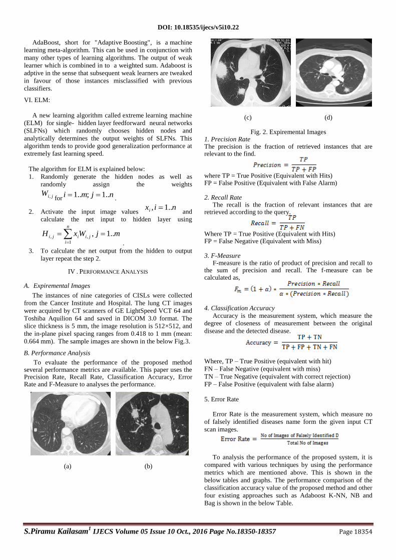
Methods Error Rate Value
Adaboost 15%
K-NN 13%
NB 11%
Bag 8%
SVM 5%
ELM 3%
The performance comparison of the error rate value of the
proposed method and other four existing approaches such as
Adaboost K-NN, NB and Bag is shown in the below Fig.4.
The error rate value of the five methods including the
proposed method is given and then it is compared. The error
rate value of the ELM method is lower than the other method.
The Error Rate value of the proposed method is less than the
other four existing approaches. It is clearly shown in the above
Fig.5. Because of the lower error rate the proposed method is
best than the other four existing approaches.
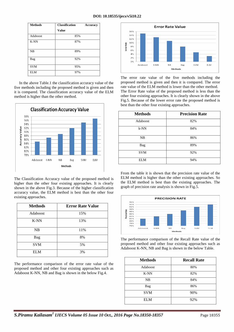
Methods Precision Rate
Adaboost 82%
k-NN 84%
NB 86%
Bag 89%
SVM 92%
ELM 94%
From the table it is shown that the precision rate value of the
ELM method is higher than the other existing approaches. So
the ELM method is best than the existing approaches. The
graph of precision rate analysis is shown in Fig.5.
The performance comparison of the Recall Rate value of the
proposed method and other four existing approaches such as
Adaboost K-NN, NB and Bag is shown in the below Table.
Methods Recall Rate
Adaboost 80%
K-NN 82%
NB 84%
Bag 86%
SVM 90%
ELM 92%
DOI: 10.18535/ijecs/v5i10.22
S.Piramu Kailasam1 IJECS Volume 05 Issue 10 Oct., 2016 Page No.18350-18357 Page 18356
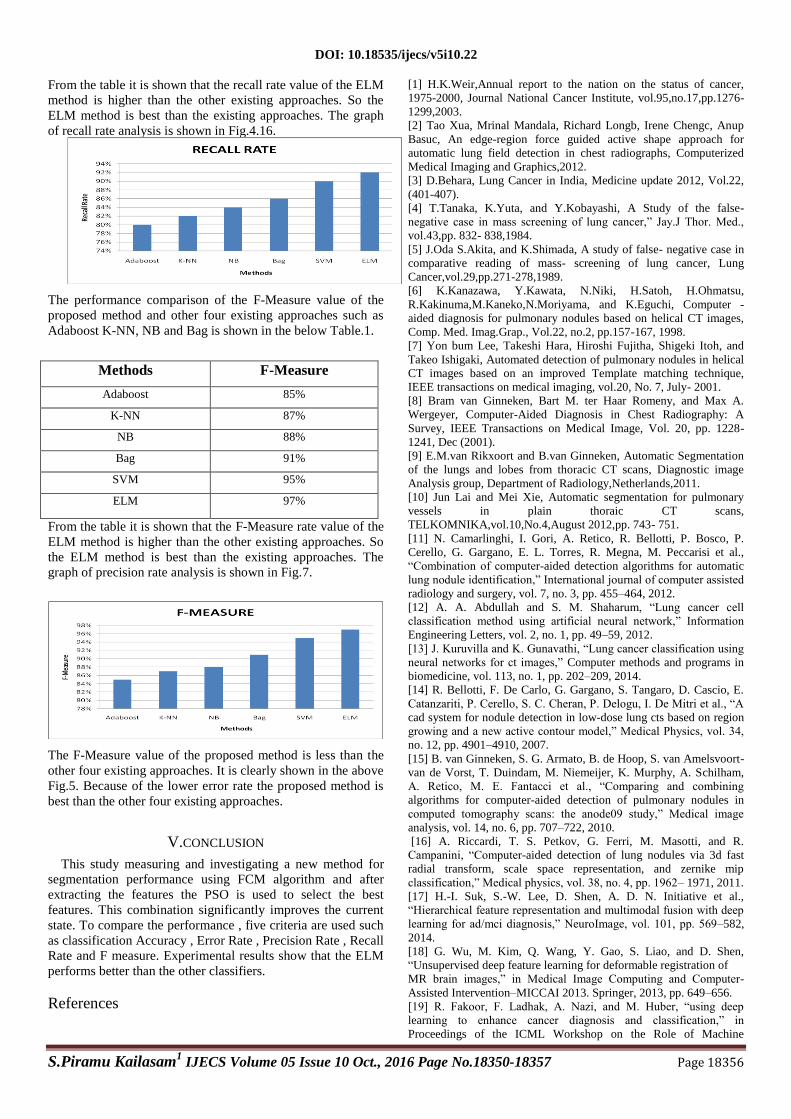
From the table it is shown that the recall rate value of the ELM
method is higher than the other existing approaches. So the
ELM method is best than the existing approaches. The graph
of recall rate analysis is shown in Fig.4.16.
The performance comparison of the F-Measure value of the
proposed method and other four existing approaches such as
Adaboost K-NN, NB and Bag is shown in the below Table.1.
Methods F-Measure
Adaboost 85%
K-NN 87%
NB 88%
Bag 91%
SVM 95%
ELM 97%
From the table it is shown that the F-Measure rate value of the
ELM method is higher than the other existing approaches. So
the ELM method is best than the existing approaches. The
graph of precision rate analysis is shown in Fig.7.
The F-Measure value of the proposed method is less than the
other four existing approaches. It is clearly shown in the above
Fig.5. Because of the lower error rate the proposed method is
best than the other four existing approaches.
V.CONCLUSION
This study measuring and investigating a new method for
segmentation performance using FCM algorithm and after
extracting the features the PSO is used to select the best
features. This combination significantly improves the current
state. To compare the performance , five criteria are used such
as classification Accuracy , Error Rate , Precision Rate , Recall
Rate and F measure. Experimental results show that the ELM
performs better than the other classifiers.
References
[1] H.K.Weir,Annual report to the nation on the status of cancer,
1975-2000, Journal National Cancer Institute, vol.95,no.17,pp.1276-
1299,2003.
[2] Tao Xua, Mrinal Mandala, Richard Longb, Irene Chengc, Anup
Basuc, An edge-region force guided active shape approach for
automatic lung field detection in chest radiographs, Computerized
Medical Imaging and Graphics,2012.
[3] D.Behara, Lung Cancer in India, Medicine update 2012, Vol.22,
(401-407).
[4] T.Tanaka, K.Yuta, and Y.Kobayashi, A Study of the false-
negative case in mass screening of lung cancer,‖ Jay.J Thor. Med.,
vol.43,pp. 832- 838,1984.
[5] J.Oda S.Akita, and K.Shimada, A study of false- negative case in
comparative reading of mass- screening of lung cancer, Lung
Cancer,vol.29,pp.271-278,1989.
[6] K.Kanazawa, Y.Kawata, N.Niki, H.Satoh, H.Ohmatsu,
R.Kakinuma,M.Kaneko,N.Moriyama, and K.Eguchi, Computer -
aided diagnosis for pulmonary nodules based on helical CT images,
Comp. Med. Imag.Grap., Vol.22, no.2, pp.157-167, 1998.
[7] Yon bum Lee, Takeshi Hara, Hiroshi Fujitha, Shigeki Itoh, and
Takeo Ishigaki, Automated detection of pulmonary nodules in helical
CT images based on an improved Template matching technique,
IEEE transactions on medical imaging, vol.20, No. 7, July- 2001.
[8] Bram van Ginneken, Bart M. ter Haar Romeny, and Max A.
Wergeyer, Computer-Aided Diagnosis in Chest Radiography: A
Survey, IEEE Transactions on Medical Image, Vol. 20, pp. 1228-
1241, Dec (2001).
[9] E.M.van Rikxoort and B.van Ginneken, Automatic Segmentation
of the lungs and lobes from thoracic CT scans, Diagnostic image
Analysis group, Department of Radiology,Netherlands,2011.
[10] Jun Lai and Mei Xie, Automatic segmentation for pulmonary
vessels in plain thoraic CT scans,
TELKOMNIKA,vol.10,No.4,August 2012,pp. 743- 751.
[11] N. Camarlinghi, I. Gori, A. Retico, R. Bellotti, P. Bosco, P.
Cerello, G. Gargano, E. L. Torres, R. Megna, M. Peccarisi et al.,
―Combination of computer-aided detection algorithms for automatic
lung nodule identification,‖ International journal of computer assisted
radiology and surgery, vol. 7, no. 3, pp. 455–464, 2012.
[12] A. A. Abdullah and S. M. Shaharum, ―Lung cancer cell
classification method using artificial neural network,‖ Information
Engineering Letters, vol. 2, no. 1, pp. 49–59, 2012.
[13] J. Kuruvilla and K. Gunavathi, ―Lung cancer classification using
neural networks for ct images,‖ Computer methods and programs in
biomedicine, vol. 113, no. 1, pp. 202–209, 2014.
[14] R. Bellotti, F. De Carlo, G. Gargano, S. Tangaro, D. Cascio, E.
Catanzariti, P. Cerello, S. C. Cheran, P. Delogu, I. De Mitri et al., ―A
cad system for nodule detection in low-dose lung cts based on region
growing and a new active contour model,‖ Medical Physics, vol. 34,
no. 12, pp. 4901–4910, 2007.
[15] B. van Ginneken, S. G. Armato, B. de Hoop, S. van Amelsvoort-
van de Vorst, T. Duindam, M. Niemeijer, K. Murphy, A. Schilham,
A. Retico, M. E. Fantacci et al., ―Comparing and combining
algorithms for computer-aided detection of pulmonary nodules in
computed tomography scans: the anode09 study,‖ Medical image
analysis, vol. 14, no. 6, pp. 707–722, 2010.
[16] A. Riccardi, T. S. Petkov, G. Ferri, M. Masotti, and R.
Campanini, ―Computer-aided detection of lung nodules via 3d fast
radial transform, scale space representation, and zernike mip
classification,‖ Medical physics, vol. 38, no. 4, pp. 1962– 1971, 2011.
[17] H.-I. Suk, S.-W. Lee, D. Shen, A. D. N. Initiative et al.,
―Hierarchical feature representation and multimodal fusion with deep
learning for ad/mci diagnosis,‖ NeuroImage, vol. 101, pp. 569–582,
2014.
[18] G. Wu, M. Kim, Q. Wang, Y. Gao, S. Liao, and D. Shen,
―Unsupervised deep feature learning for deformable registration of
MR brain images,‖ in Medical Image Computing and Computer-
Assisted Intervention–MICCAI 2013. Springer, 2013, pp. 649–656.
[19] R. Fakoor, F. Ladhak, A. Nazi, and M. Huber, ―using deep
learning to enhance cancer diagnosis and classification,‖ in
Proceedings of the ICML Workshop on the Role of Machine
DOI: 10.18535/ijecs/v5i10.22
S.Piramu Kailasam1 IJECS Volume 05 Issue 10 Oct., 2016 Page No.18350-18357 Page 18357
Learning in Transforming Healthcare (WHEALTH). Atlanta, GA,
2013.
[20] D. Zinovev, J. Feigenbaum, J. Furst, and D. Raicu, ―Probabilistic
lung nodule classification with belief decision trees,‖ in Engineering
in Medicine and Biology Society, EMBC, 2011 Annual International
Conference of the IEEE. IEEE, 2011, pp. 4493–4498.

See discussions, stats, and author profiles for this publication at: https://www.researchgate.net/publication/348336445
Traffic flow Prediction with Big Data Using SAE'S Algorithm
Article · July 2016
CITATIONS
2READS
172
3 authors, including:
Some of the authors of this publication are also working on these related projects:
Fuzzy methods View project
Deep Learning Algorithms View project
Piramu Kailasam
Sadakathullah Appa College
16 PUBLICATIONS 12 CITATIONS
SEE PROFILE
Mohamed Sathik
Sadakathullah Appa College
119 PUBLICATIONS 789 CITATIONS
SEE PROFILE
All content following this page was uploaded by Piramu Kailasam on 08 January 2021.
The user has requested enhancement of the downloaded file.

S.Piramu Kailasam et al, International Journal of Computer Science and Mobile Computing, Vol.5 Issue.7, July- 2016, pg. 186-193
© 2016, IJCSMC All Rights Reserved 186
Available Online at www.ijcsmc.com
International Journal of Computer Science and Mobile Computing
A Monthly Journal of Computer Science and Information Technology
ISSN 2320–088X IMPACT FACTOR: 5.258
IJCSMC, Vol. 5, Issue. 7, July 2016, pg.186 – 193
Traffic flow Prediction with Big Data
Using SAE’S Algorithm
S.Piramu Kailasam (Ph.d), K.Aruna Anushiya, Dr. M.Mohammed Sathik ¹Research Scholar, Bharathiar University, India
²Assistant Professor, MSU College, India 3Principal, Sadakathullah Appa College, Tirunelveli, India
1 [email protected]; 2 [email protected]
Abstract— Intelligent transportation system is accurate and time based traffic flow information to do best
performance . Last few years, traffic data have been huge, existing system used weak traffic prediction
models which is unsatisfied. The proposed system is using novel deep learning based traffic flow prediction
method, which involves the spatial and temporal correlations inherently. A stack autoencoder model is used
to learn generic traffic flow features and it is trained in a greedy layerwise pattern. This is the first time that a
deep architecture model is proposed using autoencoders to represent traffic flow features for prediction.
Keywords— Deep learning, stacked autoencoders (SAEs), traffic flow prediction.
I. INTRODUCTION
The traffic flow information is [1] the potential to help road users, which make better travel decisions in
traffic congestion and reduce carbon emissions. This will improve traffic operation efficiently. Now days
transportation management system and control becomes more complicated data driven. The most of the Traffic
flow predication system method is used shallow traffic model which are unsatisfied. Deep learning , which is a
type of machine learning method, has a lot of interest academic and industrial level.
Deep learning algorithms use multiple-layer architectures to extract inherent features in data from the lowest
to the highest level using deep learning algorithm. Without prior knowledge, we can represent the traffic
feature which has good performance in traffic flow prediction.
II. LITERATURE REVIEW
A Traffic flow prediction is a key functional component in ITSs. A countable traffic flow prediction models
have been developed to assist in traffic management .These models will control and improving transportation
efficiency ranging from route guidance and vehicle routing . The traffic flow can be considered a temporal and
spatial process. The traffic flow prediction problem can be stated as follows. Let Xt i denote the observed traffic
flow quantity during the tth time interval at the ith observation location in a transportation network. Given a
sequence {Xt i} of observed traffic flow data, i = 1, 2, . . . , m, t = 1, 2, . . . , T , the problem is to predict the traffic flow at time interval (t+Δ) for some prediction horizon Δ. As early as 1970s, the autoregressive integrated
moving average (ARIMA) model was used to predict short-term freeway traffic flow [3]. The variety of models
for traffic flow prediction have been proposed by researchers from different areas, such as transportation

S.Piramu Kailasam et al, International Journal of Computer Science and Mobile Computing, Vol.5 Issue.7, July- 2016, pg. 186-193
© 2016, IJCSMC All Rights Reserved 187
engineering, statistics, machine learning, control engineering, and economics. Previous prediction approaches
can be grouped into three categories, i.e., parametric techniques, nonparametric methods, and simulations.
Parametric models include time-series models, Kalman filtering models, etc. Nonparametric models include k-
nearest neighbor (k-NN) methods, artificial neural networks (ANNs), etc. Simulation approaches use traffic
simulation tools to predict traffic flow.
A widely used technique to the problem of traffic flow prediction is based on time-series methods, a local linear
regression model for short-term traffic forecasting[22]. A Bayesian network approach was proposed for traffic
flow forecasting in [23]. An online learning weighted support vector regression (SVR) was presented in [24] for
short-term traffic flow predictions. Various ANN models were developed for predicting traffic flow. It is
difficult to say that one method is clearly superior over other methods in any situation. One reason for this is that
the proposed models are developed with a small amount of separate specific traffic data, and the accuracy of
traffic flow prediction methods is dependent on the traffic flow features embedded in the collected spatiotemporal traffic data. Moreover, in general, literature shows promising results when using NNs, which
have good prediction power and robustness. Although the deep architecture of NNs can learn more powerful
models than shallow networks, existing NN-based methods for traffic flow prediction usually only have one
hidden layer. It is hard to train a deep-layered hierarchical NN with a gradient-based training algorithm. Recent
advances in deep learning have made training the deep architecture feasible since the breakthrough of Hinton ,
and these show that deep learning models have superior or comparable performance with state-of-the-art
methods in some areas. In this paper, we explore a deep learning approach with SAEs for traffic flow prediction.
III. METHODOLOGY
In proposed system SAE’s model is introduced SAE is Stacked Autoencoder. The SAE is an Neural network
that attempt to reduce its input. Fig.1 gives the details of auto encoder, which has one input layer, one hidden
layer and one output layer. A set of training samples
{x(1), x(2), x(3), . . .}, where x(i) ∈ Rd, an autoencoder first encodes an input x(i) to a hidden representation
y(x(i)) based on (1), and then it decodes representation y(x(i)) back into a reconstruction z(x(i)) computed as (2).
y(x) =f(W1x + b) (1)
z(x) =g (W2y(x) + c) (2)
where
W1 is a weight matrix,
b is an encoding bias vector,
W2 is a decoding matrix, and
c is a decoding bias vector.
Fig.2. Layerwise training of SAEs.
When sparsity constraints are added to the objective function, an autoencoder becomes a sparse autoencoder.
This encoder considers the sparse representation of the hidden layer. To obtain the sparse representation, we will reconstruct the error.

S.Piramu Kailasam et al, International Journal of Computer Science and Mobile Computing, Vol.5 Issue.7, July- 2016, pg. 186-193
© 2016, IJCSMC All Rights Reserved 188
Where
γ is the weight of the sparsity term,
ρ is a sparsity parameter
ρj = average activation of hidden unit
KL(ρ_ˆρj) - is the Kullback–Leibler (KL) divergence
SAEs A SAE model is created by stacking autoencoders to form a deep network by taking the output of the
autoencoder found on the layer below as the input of the current layer .The l- layers in SAE, the first layer is
trained as an autoencoder, with the training set as inputs. After obtaining the first hidden layer, the output of the
kth hidden layer is used as the input of the (k + 1)th hidden layer, multiple autoencoders can be stacked
hierarchically. This is shows in Fig. 2 By using the SAE network for traffic flow prediction, we need to add a
standard predictor on the top layer. In this paper, we put a logistic regression layer on top of the network for
supervised traffic flow prediction. The SAEs plus the predictor comprise the whole deep architecture model for
traffic flow prediction. This is showed in Fig. 3.
Fig. 3. Deep architecture model for traffic flow prediction. A SAE model is
used to extract traffic flow features, and a logistic regression layer is applied for prediction.
C. Training Algorithm
By applying the BP method with the gradient-based optimization technique. it is also known as top-down way,
that deep networks trained in this way not successful. In greedy layerwise unsupervised learning algorithm that
can train deep networks successfully. The key point to using the greedy layerwise unsupervised learning
algorithm is to pretrain the deep network layer by layer in a bottom–up way trained, fine-tuning using BP can be
applied to tune the model’s parameters in a top–down direction to obtain better output. at the same time. The
training procedure is based on the works in [58] and [59], which can be stated as follows.

S.Piramu Kailasam et al, International Journal of Computer Science and Mobile Computing, Vol.5 Issue.7, July- 2016, pg. 186-193
© 2016, IJCSMC All Rights Reserved 189
1) Train the first layer as an autoencoder by minimizing the objective function with the training sets as the
input.
2) Train the second layer as an autoencoder taking the first layer’s output as the input.
3) Iterate as in 2) for the desired number of layers.
4) Use the output of the last layer as the input for the prediction layer, and initialize its parameters randomly or
by supervised training.
5) Fine-tune the parameters of all layers with the BP method in a supervised way.
This procedure is summarized in Algorithm 1.
Algorithm 1. Training SAEs Given training samples X and the desired number of hidden
layers l,
Step 1) Pretrain the SAE — Set the weight of sparsity γ, sparsity parameter ρ, initialize weight matrices and
bias vectors randomly.
— Greedy layerwise training hidden layers.
— Use the output of the kth hidden layer as the input of the (k + 1)th hidden layer. For the first hidden
layer, the input is the training set.
— Find encoding parameters for the (k + 1)th hidden layer by minimizing the objective function.
Step 2) Fine-tuning the whole network
— Initialize randomly or by supervised training like ,
— Use the BP method with the gradient-based optimization technique to change the
whole network’s parameters in a top–down fashion.
Data Description
The proposed deep architecture model was applied to the data collected from the Caltrans Performance
Measurement System (PeMS) database as a numerical example. The traffic data are collected every 30 s from over 15000 individual detectors, which are deployed statewide in freeway systems . The collected data are
aggregated 5-min interval each for each detector station. In this paper, the traffic flow data collected in the
weekdays of the first three months of the year 2013 were used for the experiments. The data of the first two
months were selected as the training set, and the remaining one month’s data were selected as the testing set.
For freeways with multiple detectors, the traffic data collected by different detectors are aggregated to get the
average traffic flow of this freeway. Note that we separately treat two directions of the same freeway among all
the freeways, in which three are one-way. Fig. 4 is a plot of a typical freeway’s traffic flow over time for
weekdays of some week.
Experiments :
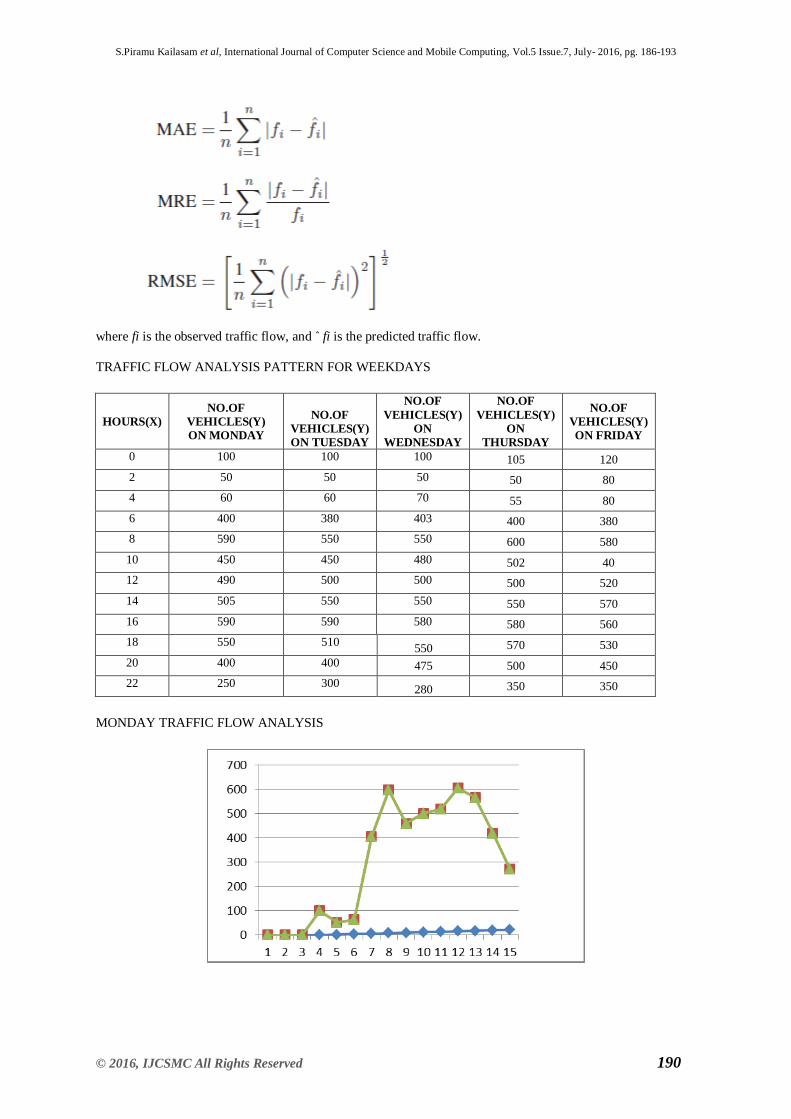
we use three performance indexes, which are the mean absolute error (MAE), the mean relative error (MRE), and the RMS error(RMSE).
RESULT
We compared the Index of Performance
To evaluate the effectiveness of the proposed model, we use three performance indexes, which are the mean
absolute error (MAE), the mean relative error (MRE), and the RMS error (RMSE) they are define as
S.Piramu Kailasam et al, International Journal of Computer Science and Mobile Computing, Vol.5 Issue.7, July- 2016, pg. 186-193
© 2016, IJCSMC All Rights Reserved 190
where fi is the observed traffic flow, and ˆ fi is the predicted traffic flow.
TRAFFIC FLOW ANALYSIS PATTERN FOR WEEKDAYS
HOURS(X)
NO.OF
VEHICLES(Y)
ON MONDAY
NO.OF
VEHICLES(Y)
ON TUESDAY
NO.OF
VEHICLES(Y)
ON
WEDNESDAY
NO.OF
VEHICLES(Y)
ON
THURSDAY
NO.OF
VEHICLES(Y)
ON FRIDAY
0 100 100 100 105 120
2 50 50 50 50 80
4 60 60 70 55 80
6 400 380 403 400 380
8 590 550 550 600 580
10 450 450 480 502 40
12 490 500 500 500 520
14 505 550 550 550 570
16 590 590 580 580 560
18 550 510 550 570 530
20 400 400 475 500 450
22 250 300 280 350 350
MONDAY TRAFFIC FLOW ANALYSIS

S.Piramu Kailasam et al, International Journal of Computer Science and Mobile Computing, Vol.5 Issue.7, July- 2016, pg. 186-193
© 2016, IJCSMC All Rights Reserved 191
TUESDAY TRAFFIC FLOW ANALYSIS
WEDNESDAY TRAFFIC FLOW ANALYSIS
THURSDAY TRAFFIC FLOW ANALYSIS

S.Piramu Kailasam et al, International Journal of Computer Science and Mobile Computing, Vol.5 Issue.7, July- 2016, pg. 186-193
© 2016, IJCSMC All Rights Reserved 192
FRIDAY TRAFFIC FLOW ANALYSIS
IV. CONCLUSIONS
The Era of Big data is an urgent need for advanced data acquisition, management and analysis. In this paper
we have presented the concept of big data and highlighted the big data value chain. The proposed method
discovered the traffic flow feature representation as the nonlinear spatial and temporal correlations from the
traffic data. We used the greedy layerwise unsupervised learning algorithm to pretrain the large network and
improve the prediction performance. We assessed the performance of the proposed method and compared with
BP NN, RBF NN, RW and SVM models and the result show that the proposed method is better than the other
method. Future work, it would be interesting to find deep learning algorithm for traffic flow prediction.
he version of this template is V2. Most of the formatting instructions in this document have been compiled by Causal Productions from the IEEE LaTeX style files. Causal Productions offers both A4 templates and US
Letter templates for LaTeX and Microsoft Word. The LaTeX templates depend on the official IEEEtran.cls and
IEEEtran.bst files, whereas the Microsoft Word templates are self-contained. Causal Productions has used its
best efforts to ensure that the templates have the same appearance.
REFERENCES [1] N. Zhang, F.-Y. Wang, F. Zhu, D. Zhao, and S. Tang, ―DynaCAS: Computational experiments and
decision support for ITS,‖ IEEE Intell. Syst.,vol. 23, no. 6, pp. 19–23, Nov./Dec. 2008.
[2] J. Zhang et al., ―Data-driven intelligent transportation systems: A survey,‖IEEE Trans. Intell. Transp. Syst.,
vol. 12, no. 4, pp. 1624–1639, Dec. 2011. [3] M. S. Ahmed and A. R. Cook, ―Analysis of freeway traffic time-series data by using Box–Jenkins
techniques,‖ Transp. Res. Rec., no. 722, pp. 1–9,1979.
[4] M. Levin and Y.-D. Tsao, ―On forecasting freeway occupancies and volumes,‖Transp. Res. Rec., no. 773,
pp. 47–49, 1980.
[5] M. Hamed, H. Al-Masaeid, and Z. Said, ―Short-term prediction of traffic volume in urban arterials,‖ J.
Transp. Eng., vol. 121, no. 3, pp. 249–254,May 1995.
[6] M. vanderVoort, M. Dougherty, and S. Watson, ―Combining Kohonen maps with ARIMA time series
models to forecast traffic flow,‖ Transp.Res. C, Emerging Technol., vol. 4, no. 5, pp. 307–318, Oct. 1996.
[7] S. Lee and D. Fambro, ―Application of subset autoregressive integrated moving average model for short-
term freeway traffic volume forecasting,‖Transp. Res. Rec., vol. 1678, pp. 179–188, 1999.
[8] B. M. Williams, ―Multivariate vehicular traffic flow prediction—Evaluation of ARIMAX modeling,‖ Transp. Res. Rec., no. 1776, pp. 194–200, 2001.
[9] Y. Kamarianakis and P. Prastacos, ―Forecasting traffic flow conditions in an urban network—Comparison
of multivariate and univariate approaches,‖Transp. Res. Rec., no. 1857, pp. 74–84, 2003, Transporation
Network Modeling 2003: Planning and Administration.
[10] H. Y. Sun, H. X. Liu, H. Xiao, R. R. He, and B. Ran, ―Use of local linear regression model for short-term
traffic forecasting,‖ Transp. Res. Rec.,no. 1836, pp. 143–150, 2003, Initiatives in Information Technology
and Geospatial Science for Transportation: Planning and Administration.

S.Piramu Kailasam et al, International Journal of Computer Science and Mobile Computing, Vol.5 Issue.7, July- 2016, pg. 186-193
© 2016, IJCSMC All Rights Reserved 193
[11] S. Sun, C. Zhang, and Y. Guoqiang, ―A Bayesian network approach to traffic flow forecasting,‖ IEEE
Intell. Transp. Syst. Mag., vol. 7, no. 1,pp. 124–132, Mar. 2006.
[12] Y. S. Jeong, Y. J. Byon, M. M. Castro-Neto, and S. M. Easa, ―Supervised weighting-online learning
algorithm for short-term traffic flow prediction,‖ IEEE Trans. Intell. Transp. Syst., vol. 14, no. 4, pp.
1700–1707,Dec. 2013.
View publication statsView publication stats

S. Piramu Kailasam et al, International Journal of Computer Science and Mobile Computing, Vol.5 Issue.7, July- 2016, pg. 194-203
194 © 2016, IJCSMC All Rights Reserved
Available Online at www.ijcsmc.com
International Journal of Computer Science and Mobile Computing
A Monthly Journal of Computer Science and Information Technology
ISSN 2320–088X IMPACT FACTOR: 5.258
IJCSMC, Vol. 5, Issue. 7, July 2016, pg.194 – 203
Guidance in Assisting the
Identification / Interpretation of
Lung Cancer using Bronchoscope
S. Piramu Kailasam1, Dr. M.Mohammed Sathik2
¹Research Scholar, Bharathiyar University, Coimbatore, India ²Principal, Sadakathullah Appa College, Tirunelveli, India
Abstract— Lung Cancer is one of the leading disease in the world, and increased in many countries. The
eight year overall survival rate is just 17%. We have to remove lung cancer surgically at an early stage to
ensure the survival of the patient. There are several methods to treat an early staged lung cancer such as
Brachytherapy, Cryotherapy, Photodynamic therapy, Argon plasma cogulation, Thermal laser, micro
debrider, electrocautery etc. In this review we are going to discuss various types of bronchoscopy and their
positive and negative sides.
Keywords— Lung cancer, bronchoscopy
I. INTRODUCTION
The first sign of evolution of bronchoscope was apparent when a German physician, Gustav killian removed a
pork bone from the right main bronchus of a Black forest worker in the year 1897. He had used a similar device
with the same limitations as that of a modern bronchoscope includes two types of devices – rigid and flexible
each having their own positives and negatives.
II. CHOOSING BRONCHOSCOPY
Bronchoscopic treatment is advisible for treating only lung cancer at an early stage. But bronchoscopy is a cost effective treatment. The patient undergoing treatment should not have low life expectancy. These are
some criteria for choosing bronchoscopy. Let us decide which bronchoscopy to choose rigid or flexible. Rigid
bronchoscopy is defined as trans oral or trans tracheosomy passage of rigid instruments for diagnosis or therapy
aided by various light sources, telescopes and instruments , requiring a general anaesthetic.
Flexible bronchoscopy is defined as a technical procedure that is utilized to visualize the nasal passage
from nasal opening to bronchial tree end which is usually carried out under conscious sedation.
Mostly a flexible bronchoscopy is preferable because a rigid brochoscopy requires a lot of skill.
Majority of doctors in US and UK lack this skill. But there are some circumstances in which rigid bronchoscopy
is advisable.

S. Piramu Kailasam et al, International Journal of Computer Science and Mobile Computing, Vol.5 Issue.7, July- 2016, pg. 194-203
195 © 2016, IJCSMC All Rights Reserved
Unstable patients, those with significant underlying cardio pulmonary disease, uncontrolled coagulapathy and
those with cervical instability need to be carefully assessed. Mortality from flexible bronchoscopy is rarer than
with rigid bronchoscopy. Rigid bronchoscopy requires a skilled anaesthesiologist support.
A. Comparative study of different bronchoscopical methods
TABLE I
Types of
broncho
sco py
/charac-
teri stics
Electrocau
ter y
Argon
Plasma
Coagulation
Thermal
laser
Micro-
deb rider
Cryo
therap y
Brachy
ther apy
Phtoto
dyna mic
therapy
Indication Hemoptysis, Debulking of
endobronchial tumor
Hemoptysis, Debulking of
endobronchia l tumor
Debulking of endobronchial
tumor
Debulking of endobronc
hial tumor
Debulking of endobron
chial tumor
Treatment of endobron-
chi al or
Peribron-chia l tumor
Treatment of endobron
chi al or
peribron- chia l tumor
Effect Immediate Immediate Immediate Immediate Delayed Delayed Delayed
Rigid or Flexible
Both Both Both Rigid Both Both Both
Caution and Contraindic
-ation
Pace maker or defibrillators
Fio2 of
>
0.4(burns)
Per Electrocauter y
Fio2<0.4 Contraindica- tion No exphytic lesion visible.
Total airway obstruction and no
functional distal airway open
None
Distal lesion
None
Acute airway Obstruction requiring immediate relief
Expensive
Healthcare worker shielding Treatment for malignant
tracheoeso-
phageal fistula
Skin photo-sensitivity for several weeks Massive
hemop-tysis, Bronchople ural fistula, Subepithelia l fibrosis
B. Advances in Therapy
Using Bronchoscopy (Immediate Effect)
1) Electrocautery: Electrocautery uses a high frequency electrical current which causes a heating of
the tissues that the probe is with contact. Coagulation is achieved in low voltage and tissue will be
vaporized in high voltages. The difficulties of endobronchial electrocautery include that of general
bronchoscopy. Application of deep electrocautery too close to the bronchial well may result in perforation
and pneunothromax. Electrocautery is a safe, cheap and effective therapy for early stage and advanced cancer with MAO(Malignant Airway Obstruction).
2) Argon Plasma Coagulation: Argon Plasma Coagulation has to resect MAO and to control
endobronchial bleeding . A beam of argon gas acts as a non contact for the electrocautery effect which
distinguishes APC from electrocautery. APC is a cheap , safe and effective modality for treating both
MAO and hemoptysis.
3) Laser: A Laser in bronchoscopy started almost thirty years ago. Bronchoscopic laser resection is a
useful modality in the treatment of MAO. Airway obstruction to bronchogenic cascinoma is the most
frequent indication for laser resection.The tumor is removed by two methods,
1. Resection
2. Vaporization

S. Piramu Kailasam et al, International Journal of Computer Science and Mobile Computing, Vol.5 Issue.7, July- 2016, pg. 194-203
196 © 2016, IJCSMC All Rights Reserved
In the first one the laser is aimed at the target lesion and through photocoagulation of the feeding blood
vessels and amelioration of the lesion the devitalized tissue is removed through the bronchoscope.
The second, which is vaporization involves aligning the laser parallel to the bronchial wall and aiming
at the edge of the intraluminal lesion. Laser pulses have limits to 1s or less. The laser is used in parallel with the
target lesion and not straight on or perpendicular to reduce the chances of perforation.
A Cheaper endobronchial laser is now a days available. [neodymium:yttrium-aluminum
perovskite(Nd:YAP)] . One study of 133patients with various malignant and benign(7 patients) indications
concluded that the Nd:YAP laser was a safe and effective tool for bronchoscopy.
Laser through bronchoscopy is an effective approach for treatment MAO. ND:YAG laser is expensive. It needs
trained staff to operate with safety to prevent injury to patients.
4) Microdebridement:
A microdebridement operates by using a powered rotating blade and a simultaneously operating
suction device to facilitate the removal of debris.
The elongated rotating tip microdebrider to about 45cm is the special and it is accurate and allows high
flow oxygen. The comblications of thermal such as airway injury, airway fires, tracheoessophgeal fistuals can
be avoided using micro debridement. The complications are hemorrhage, perforation and pneumothorax.
Delayed effect: (Cryotherapy)
In 1812 during Russian Campaign , cryotherapy is a cheap and effective treatment for many medical
conditions. The bronchoscopic cryotherapy is a procedure where, either through rigid or flexible bronchoscopy, malignant or benign tissue is ablated by repeatedly freezing , thawing and refreezing. Cryotherapy may be
considered for MAO in patients without critical airway narrowing . Main advantages is no limitation in oxygen
delivery during the procedure.
Brachytherapy is an invasive two step technique. The first step is to identify the target lesion and the
second step is to remotely under fluoroscopy and computer guidance. Place the radioactive source beside the
target lesion and also changes in its position in a staged process to allow irradiation on the target lesion.
Irridium 192 is the most common isotope used because it permits a dramatic reduction of treatment
time reduces costs, enhances the patient experience and allows for an outpatient setting over several sessions.
Lowdose Rate is less than 2Gy/h and max of 1500 – 5000cGy over 3 days. And costly cumbersome
with radiation protection measures. HDR is about 12 Gy/h with the dose varying from 100 to 300 cGy. HDR is
less costly than LDR and enhances the patient experience.
Brachytherapy is effective in the palliation of both endobronchial and peribronchial malignancy with a
delayed effect. Significant risk of hemoptysis is found.
5) Photo dynamic Therapy:
Skin cancers can be treated by photodynamic therapy. This therapy has a successful record for malignant and benign conditions.
PDT has been combined with other endobronchial therapies, including brachytherapy therapies which are brachytherapy and laser therapy. Complication of PDT are sunburn upto 6 weeks post HPD administration is a concern and patients need to be fully informed to avoid sunlight and to wear appropriate clothing.
PDT is effective in debulking and palliation with delayed effect and no limitation of oxygenation in MAO.
C. Airway stents
Tracheobronchial prostheses or Airway stents are tube shaped devices that are inserted into an airway
to maintain airway patency. These are made of metal , silicone or other meterials can be used to relieve airway obstruction caused be malignant tumors.
Stent therapy is indicated in both intraluminal and extraluminal major airway obstructions.
After removal of endobronchial obstruction stents can be considered to maintain airway patency. Self
expandable metal stents should not be placed in patients where removal is considered in future.
S. Piramu Kailasam et al, International Journal of Computer Science and Mobile Computing, Vol.5 Issue.7, July- 2016, pg. 194-203
197 © 2016, IJCSMC All Rights Reserved
D. Techniques in Bronchoscopy
1) Genomic classifier for lung cancer by diagnostic bronchoscopy
Low Dose Computed Tomography (CT) screening results in a 20% relative mortality reduction in high
risk[2]. The gene expression profile of cyto logically normal bronchial airway epithelial cells has been shown to
be altered in patients with lung cancer. A gene expression classifier from airway epithelial cells that detects the
presence of cancer in smokers. Bronchoscopy suspect lung cancer and evaluated its sensitivity to detect lung
cancer among patients from an independent cohort. Bronchoscopy is considered to be safer than other invasive
sampling methods such as transthoracic needle biopsy(TTNB) or surgical techniques[3].
Lung Cancer – related genes were selected and a classifier for predicting the likelihood of lung cancer based on the combination of the cancer genes, the gene expression correlates and patient age was derived. All aspects of this classifier development procedure were determined using cross validation and using only data from the training set samples.
A logistic regression model with lung cancer status (cancer positive = 1 and cancer negative = 0) as the dependent variable was fit using the training data clinical factor gene expression correlates and patient age as
predictors. This severed as the baseline for subsequence gene analysis.
The classifier adds substantial sensitivity the bronchoscopy procedure resulting in high NPV. This can
be used to aid in decision making when bronchoscopy is non diagnostic by identifying patients who are at low
risk of having lung cancer. ROC curve analysis of the training set cohort using the finalized gene expression classifier is evaluated.
Classifier accuracy was measured by the area under the curve, sensitivity, specificity, NPV and PPV ,
cross validation using a 10% sample hold-out set[4].
TABLE III
Sensitivity of Bronchoscopy , the classifier and Combined procedures comparison by size
Mass size N Bronchoscopy sensitivity Classifier sensitivity Combined sensitivity
< 3 cm 99 44% 87% 93%
>3 cm 48 58% 94% 98%
Infiltrate 16 38% 100% 100%
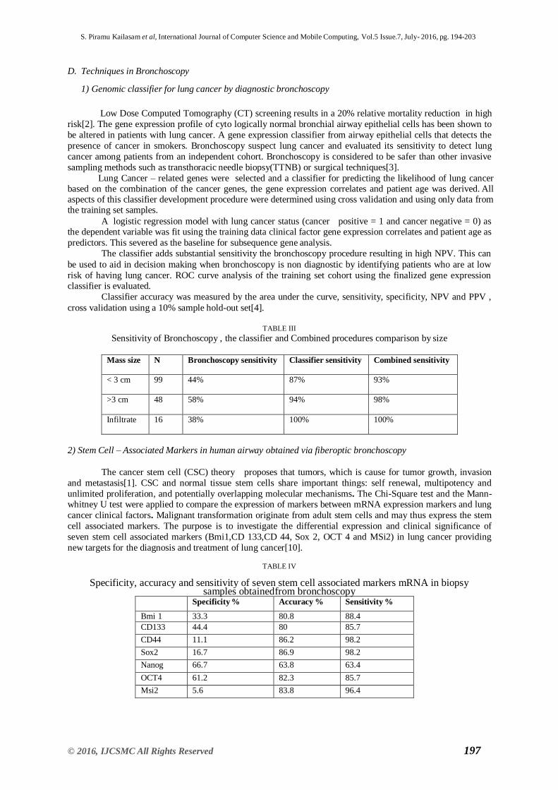
2) Stem Cell – Associated Markers in human airway obtained via fiberoptic bronchoscopy
The cancer stem cell (CSC) theory proposes that tumors, which is cause for tumor growth, invasion
and metastasis[1]. CSC and normal tissue stem cells share important things: self renewal, multipotency and
unlimited proliferation, and potentially overlapping molecular mechanisms. The Chi-Square test and the Mann- whitney U test were applied to compare the expression of markers between mRNA expression markers and lung
cancer clinical factors. Malignant transformation originate from adult stem cells and may thus express the stem
cell associated markers. The purpose is to investigate the differential expression and clinical significance of
seven stem cell associated markers (Bmi1,CD 133,CD 44, Sox 2, OCT 4 and MSi2) in lung cancer providing
new targets for the diagnosis and treatment of lung cancer[10].
TABLE IV
Specificity, accuracy and sensitivity of seven stem cell associated markers mRNA in biopsy samples obtained from bronchoscopy
Specificity % Accuracy % Sensitivity %
Bmi 1 33.3 80.8 88.4
CD133 44.4 80 85.7
CD44 11.1 86.2 98.2
Sox2 16.7 86.9 98.2
Nanog 66.7 63.8 63.4
OCT4 61.2 82.3 85.7
Msi2 5.6 83.8 96.4

S. Piramu Kailasam et al, International Journal of Computer Science and Mobile Computing, Vol.5 Issue.7, July- 2016, pg. 194-203
198 © 2016, IJCSMC All Rights Reserved
Fig. 1 Classifiers graphical analysis
Table 3 shows the specificity, accuracy and sensitivity values of stem cell associated markers mRNA
in bronchoscopic biopsies. This has taken from lung cancer and non cancer patients.
The highest sensitivity is CD44 (98.2%), Sox2 (98.2%) and Msi2 (96.4%). But their specificity were too low to
be considered of no clinical significance. Nanog marker has the highest specificity 66.7% and the sensitivity is
63.4%. So, Bmi1,CD44 and CD133 are poor diagnostic markers for lung cancer. Nanog may serve as a
promising diagnostic marker of lung cancer and potential therapeutic target in lung cancer.
3) Optimal procedure planning for peripheral bronchoscopy
Multidetector computed tomography scanners and Ultrathin bronchoscopes, the use of bronchoscopy for diagnosing peripheral lung cancer nodules is a option[7]. Image based planning and guidance
system improves upon other systems.
TABLE .V
Collection of Target ROI sites
SITE TYPE RUL RML RLL LUL LLL TOTAL
NODULE(< 3 cm) 4 5 3 9 1 22
MASS (>3 cm) 0 1 0 3 0 4
INFILTRATE 5 2 4 4 1 16
GGO 0 0 2 1 0 3
BAL site 3 1 0 0 0 4
Lymph Node 3 1 1 2 0 7
Other 3 2 2 3 3 13
Total 18 12 12 22 5 69

S. Piramu Kailasam et al, International Journal of Computer Science and Mobile Computing, Vol.5 Issue.7, July- 2016, pg. 194-203
199 © 2016, IJCSMC All Rights Reserved
Fig. 2 Collection of Target RoI sites
Advances are,
Optimal route planning which gives accurate airway routes to arbitrarily selected target sites.
An interactive pre bronchoscopy report enables the physician to preview in advance.
Integrates all views on one monitor during bronchoscopy
Data fusion can be done during bronchoscopic navigation and ROI localization.
Registration of the VB based guidance route with the bronchoscopic video.
As a comparison this ultrathin bronchoscopy study performed with insertion depth of 5.7 airways and a
mean time to first sample of 8:30. Thus the automated system enabled bronchoscopy over 2 airways deeper into
the airway tree periphery with a sample time that was 2 min shorter on average.
4) Algorithm for video summarization of bronchoscopy procedures
The time duration of bronchoscopy lesion findings varies considerably depending on the diagnostic
and therapeutic procedures[14]. In videobronchoscopy, the whole process can be recorded as a video sequence.
The bronchoscopist who initiates the recording process and usually chooses to archive only selected views and
sequences. Video recordings registered during bronchoscopies include a considerable number of frames of poor
quality due to blurry or unfocused images. It seems that such frames are unavoidable due to the relatively tight
endobronchial space, rapid movements of the respiratory tract.
5) Applications to biopsy path planning in virtual bronchoscopy in CT Images
The volumetric data of the human body can be measured precisely by 3D Medical imaging devices.
The CAD systems give a lot of output images in a short interval of time. It is expected to reduce doctor‟s load
and helping in accurate diagnosis. When a user inputs the target zone where there is suspicion of cancer, the
CAD system displays a sequence of anatomical names of branches. The labelling accuracy was about 90%.
6) Automatic centerline extraction for 3D virtual bronchoscopy
We have an algorithm in this paper to the automatic determination of centreline of the bronchial
branches. Centerline is the approximate centre of the bronchial tube which has maximum space for
bronchoscopy to go about. First we determine the centreline of the three dimensional virtual bronchoscopy 3D
image. Initially, a lot of end points in the binary tree which links up all centre points are constructed. Next, the
endpoints of the lung airway tips are extracted. The centreline algorithm reads all the endpoints and suggests all
the shortest paths from the start to those end points. Then , modified Digikstra[13] short path algorithm is
applied to get the centreline of the bronchus.

S. Piramu Kailasam et al, International Journal of Computer Science and Mobile Computing, Vol.5 Issue.7, July- 2016, pg. 194-203
200 © 2016, IJCSMC All Rights Reserved
7) ManiSMC – Manifold Modelling and Sequential Monte Corlo Sampler for boosting navigated bronchoscopy
We can track the bronchoscope‟s motion using ManiSMC and improve the navigation of
Bronchoscopy. There are two stages in ManiSMC system. We extend local and global regressive Mapping
method (LGRM)[16] to get bronchoscopic image sequences and construct their manifolds. With this, we can
classify the specific scenes to specific branches. Next, we employ SMC sampler to integrate the data of stage,
refine positions and orientations of bronchoscopy. Experimental results suggests that this method of navigation
is highly effective. The advantage of this method is that we do not need an additional position sensor.
8) High definition bronchoscopy
Videobronchoscopy is an essential diagnostic procedure in bronchoscopic diagonisis of lung cancer[43].
High definition (HD) and advanced real time image enhancement techniques (i-scan ) can be used to further
enhance the navigation of bronchocopy[15].
CONCLUSION
In conclusion we have highlighted the bronchoscopic options for treatment of MAO which includes
immediate and delayed effect modalities . Patient selection should exclude patients with short life expectancy
limited symptoms and inability to visualize beyond the obstruction. The decision to treat should be made with
other modalities such as external beam radiation in a multidisciplinary mode. In the optical procedure,
comparing two videos of bronchoscopy and MDCT and finalising the lesion sample we treat cancer . The NPV classifier decides when bronchoscopy is non diagnostic.
In video branchoscopy calculating DCT matrix from grayscal frame and counting nonzero elements can
classify the informative from noninformative frame.The centreline algorithm and modified Digikstra short path
algorithm is used to get the centreline of the bronchus. The SMC sampler can be integrate the data of stage ,
refine orientation of bronchoscopy. Navigation of bronchoscopy can be enhanced by HD and iscan.
REFERENCES
[1] Reya T, Morrison SJ .clarke MF , Weissman IL , Stem cells, cancer and cancer stem cells.Nature
2001,414:105-111.
[2] The National lung screening trial research team, reduced lung cancer motality with lowdose computed tomographic screening. N Engl J Med,2011 ; 365-409
[3] Ernst A, Silvestri G, Johnstone D Interventional pulmonary procedures guidelines from the American
college of chest physicians . Chest 2003;123;1693-717
[4] Golub TR, Slonim DK, Tamayo P, Huard C, Gaasenbeek M, Mesirov JP, et al.Molecular Classification of
cancer: class discovery and class prediction by gene expression monitoring. Science. 1999;286(5439):531–7.
[5] N.C. Dalrymple, S. R.Prasad, M. W. Freckleton, and K.N. Chintapalli,”Informatics on radiology (infoRAD):
Introduction to the language of three dimensional imaging with multidetector CT,”Radiographics, Vol. 25, No.5,
Pno 1409-1428, Sep /Oct 2005.
[6] M.W. Graham,J.D.Gibbs,D.C.Conish and W.E. Higgins, “Robust 3D Airway Tree segmentation for Image
for Image Guided Peripheral Bronchoscopy” IEEE Trans . Med. Imag.,vol.29,no.4,pp.982-997,Apr 2010.
[7] J.Ueno, T. Murase, K. Yoneda, T.Tsujikawa, S.Sakiyama And Kondoh, ”3 Dimensional imaging of thoracic
disease with multidetector row CT”J.Med.invest. ,vol . 51,no. 3-4, pp , 163-170, aug 2004 [8] M.W.Graham,J.D.Gibbs, and W.E.Higgins,”Computer – based route definition system for peripheral
bronchoscopy”, J.Digital imag.,vol.25,no.2,pp.307-317,Apr.2012
[9] Patric D.Mitchell,Marcus P.Kennedy, “ Bronchoscopic Management of Malignant Airway
Obstruction”,Springer Healthcare 2014,May22,2014
[10] Laodong Li,Huina Yu,Xiaoyang Wang,”Expression of seven stem cell associated markers in human airway
biopsy specimens obtained via fiberoptic bronchoscopy”,JECCR,May 2013.
[11] Duncan H Whitney, Michael R Elashoff, Kate PortaSmith , Adam C Gower, Anil Vachani,”Derivation of a
bronchial genomic classifier for lung cancer in a prospective study of patients under going diagnostic
bronchoscopy.,BMC Medical Genomics,May 2015 [12] Kensaku Mori,Sinya Ema,Takyuki Kitasaka,Yoshito Mekada,Ichiro Ide ,”Automated Nomenclature of Bronchial Branches Extracted from CT Images and Its Application to Biopsy Path Planning in Virtual
Bronchoscopy”,Springer,2005
[13] Tsui Ying Law and Pheng Ann Heng,” Automatic Centerline Extraction for 3D Virtual
Bronchoscopy”,Springer,2000.
[14] Mikołaj I Leszczuk and Mariusz Duplaga ,”Algorithm for Video Summarization of Bronchoscopy
Procedures”,BioMedical Engineering,2011
[15] Erik HFM van der Heijden, Wouter Hoefsloot, Hieronymus WH van Hees and Olga CJ Schuurbiers,High
definition bronchoscopy: a randomized exploratory study of diagnostic value compared to standard white light
bronchoscopy and autofluorescence bronchoscopy, DOI 10.1186/s12931-015-0193-7,2015.
[16] ManiSMC: A New Method Using Manifold Modeling and Sequential Monte Carlo Sampler for Boosting

S. Piramu Kailasam et al, International Journal of Computer Science and Mobile Computing, Vol.5 Issue.7, July- 2016, pg. 194-203
201 © 2016, IJCSMC All Rights Reserved
Navigated Bronchoscopy,Xiongbiao Luo, Takayuki Kitasaka, and Kensaku Mori,Springer,2011
[17] Oh J, Hwang S, Lee J, Tavanapong W, Wong J, de Groen PC: “Informative frame classification for
endoscopy video,”Medical Image Analysis 2007, 11:110-127.
[18] Kender John R, Yeo Boon Lock: “Video scene segmentation via continuous video coherence,”. Proc IEEE
Int Conf on Computer Vision and Pattern Recognition 1998, 367-373.
[19] Adjeroh Donald A, Lee Moon-Chuen: “Scene-adaptive transform domain video partitioning,”. IEEE
Transactions on Multimedia 2004, 6(1):58-69.
[20] Aghbari Zaher Al, Kaneko Kunihiko, Akifumi Makinouchi: “Content-trajectory approach for searching
video databases,”. IEEE Transactions on Multimedia 2003, 5(4):516-531.
[21] Jianping Fan, Elmagarmid Ahmed K, Member Senior, Xingquan Zhu, Aref Walid G, Wu Lide: “Classview:
Hierarchical video shot classification, indexing, and accessing,”. IEEE Trans on Multimedia 2004, 6:70-86.
[21] Skarbek Władysław, Grzegorz Galiński, Wnukowicz Karol: “Tree Based Multimedia Indexing - a Survey,”.
Proc Krajowa Konferencja Radiokomunikacji, Radiofonii i Telewizji KKRRiT‟2004 Warszawa; 2004, 77-85,
Krajowa Konferencja Radiokomunikacji, Radiofonii i Telewizji.
[22] Chen Jau-Yuen, Taskiran Cuneyt, Albiol A, Delp E, Bouman C: “Vibe: A compressed video database
structured for active browsing and search,”. 2001.
[23] Lombardo Alfio, Morabito Giacomo, Giovanni Schembra: “Modeling intramedia and intermedia
relationships in multimedia network analysis through multiple timescale statistics,”. IEEE Transactions on Multimedia 2004,6(1):142-157.
[24] Xingquan Zhu, Aref Walid G, Fan Jianping, Catlin Ann C, Elmagarmid Ahmed K: “Medical video mining
for efficient database indexing, management and access,”. 2003.
[25] Xingquan Zhu, Jianping Fan, Aref Walid G, Elmagarmid Ahmed K: “Classminer: Mining medical video
content structure and events towards efficient access and scalable skimming,”. DMKD 2002.
[26] Vilarino F, Spyridonos P, Pujol O, Vitria J, Radeva P: “Automatic detection of intestinal juices in wireless
capsule video endoscopy,”. ICPR „06: Proceedings of the 18th International Conference on Pattern Recognition
Washington, DC, USA; 2006, 719-722, IEEE Computer Society.
[27] Choupo Anicet Kouomou, Laure Berti-Équille, Morin Annie: “Optimizing progressive query-by-example
over preclustered large image databases,”. CVDB „05: Proceedings of the 2nd international workshop on
Computer vision meets databases New York, NY, USA; 2005, 13-20, ACM.
[28] Arevalillo-Herráez Miguel, Ferri Francesc J, Domingo Juan: “A naive relevance feedback model for
content-based image retrieval using multiple similarity measures,”. Pattern Recogn 2010, 43(3):619-629.
[29] Leszczuk Mikołaj: “Analiza możliwości budowy internetowych aplikacji dostępu do cyfrowych bibliotek wideo,”. PhD thesis AGH University of Science and Technology, Faculty of Electrical Engineering, Automatics, Computer Science and Electronics, al. Mickiewicza 30, PL-30059 Krakow, Poland; 2005.
[30] Grega Michał, Leszczuk Mikołaj: “The prototype software for video summary of bronchoscopy procedures
with the use of mechanisms designed to identify, index and search,”. chapter in BRONCHOVID: The Computer
System for Bronchoscopy Laboratory Integrating the CT-Based Bronchoscopy and Transbronchial Needle-
Aspiration Biopsy Planning,Virtual Bronchoscopy, Management of the Bronchoscopic Procedures Recordings,
Automatic Image-Based Data Retrieval,Artifact and Pathology Detection and Interactive 2D & 3D Visualization
Springer-Verlag; 2010, 587-598.
[31] Duplaga Mariusz, Juszkiewicz Krzysztof, Leszczuk Mikołaj, Marek M, Papir Zdzisław: “Design of
Medical Digital Video Library,”. Proc Fourth International Workshop on Content-Based Multimedia Indexing
CBMI‟2005 Riga, Latvia; 2005, Content Based Multimedia Indexing.
[32] Lee Ho Young, Lee Ho Keun, Ha Yeong Ho: “Spatial color descriptor for image retrieval and video segmentation,”.IEEE Transactions on Multimedia 2003, 5(3):358-367.
[33] Duplaga Mariusz, Jarosław Bułat, Leszczuk Mikołaj, Socha Mirosław, Turcza Paweł, Romaniak Piotr:
“Overview of the BRONCHOVID computer system supporting bronchoscopy laboratory – medical and
technical perspective,”. In chapter in BRONCHOVID: The Computer System for Bronchoscopy Laboratory
Integrating the CT-Based Bronchoscopy and Transbronchial Needle-Aspiration Biopsy Planning, Virtual
Bronchoscopy, Management of the Bronchoscopic Procedures Recordings, Automatic Image-Based Data Retrieval, Artifact and Pathology Detection and Interactive 2D & 3D Visualization. Volume 69.
Springer-Verlag; 2010:511-522.
[34] Grega Michał, Leszczuk Mikołaj, Rafał Frączek, Duplaga Mariusz: “Algorithms for automatic recognition
of noninformative frames in video recordings of bronchoscopic procedures,”. chapter in BRONCHOVID: The
Computer System for Bronchoscopy Laboratory Integrating the CT-Based Bronchoscopy and Transbronchial
Needle-Aspiration Biopsy Planning, Virtual Bronchoscopy, Management of the Bronchoscopic Procedures
Recordings, Automatic Image-Based Data Retrieval, Artifact and Pathology Detection and Interactive 2D & 3D Visualization Springer-Verlag; 2010, 535- 545. [35] Park Sun Young, Sargent Dusty: “Colonoscopy video quality assessment using hidden Markov random
fields,”. Proc Medical Imaging 2011: Computer-Aided Diagnosis (SPIE 7963), 79632P (2011) Lake Buena
Vista, Florida, USA; 2011.

S. Piramu Kailasam et al, International Journal of Computer Science and Mobile Computing, Vol.5 Issue.7, July- 2016, pg. 194-203
202 © 2016, IJCSMC All Rights Reserved
[36] Johnson Scott B: “Tracheobronchial injury,”. In Seminars in Thoracic and Cardiovascular Surgery. Volume
20. Spring; 2008:(1):52-57.
[37] Kavuru MS, Mehta AC: “Applied Anatomy of the Airways,”. In Flexible Bronchoscopy.. 2 edition. Edited
by: Ko-Peng Wang, Ahtul C. Mehta and J. Francis Turner. Blackwell Publishing Company; 2004:.
[38] Mikrut Zbigniew, Duplaga Mariusz: “Analysis of images of bronchial tree ramifications for
summarization of brochoscopic videos,”. In chapter in BRONCHOVID: The Computer System for
Bronchoscopy Laboratory Integrating the CTBased Bronchoscopy and Transbronchial Needle-Aspiration
Biopsy Planning, Virtual Bronchoscopy, Management of the Leszczuk and Duplaga BioMedical Engineering
OnLine 2011, 10:110 Page 16 of 17 Bronchoscopic Procedures Recordings, Automatic Image-Based Data
Retrieval, Artifact and Pathology Detection and Interactive 2D & 3D Visualization. Volume 69. Springer-
Verlag; 2010:583-586.
[39] ISO/IEC: “Information technology - multimedia content description interface,” ISO/IEC 15938. 2002. [40] Janowski Lucjan, Suwada Krzysztof, Duplaga Mariusz: “Fast MPEG-7 image features-based automatic
recognition of the lesion in the bronchoscopic recordings,”. chapter in BRONCHOVID: The Computer System
for Bronchoscopy Laboratory Integrating the CT-Based Bronchoscopy and Transbronchial Needle Aspiration
Biopsy Planning, Virtual Bronchoscopy, Management of the Bronchoscopic Procedures Recordings, Automatic
Image-Based Data Retrieval, Artifact and Pathology Detection and Interactive 2D & 3D Visualization Springer-
Verlag; 2010.
[41] Pawlik Piotr, Mariusz Duplaga: “Application of SIFT image analysis method to support of transbronchial
needleaspiration biopsy,”. In chapter in BRONCHOVID: The Computer System for Bronchoscopy Laboratory
Integrating the CTBased Bronchoscopy and Transbronchial Needle-Aspiration Biopsy Planning, Virtual
Bronchoscopy, Management of the Bronchoscopic Procedures Recordings, Automatic Image-Based Data
Retrieval, Artifact and Pathology Detection and
Interactive 2D & 3D Visualization. Volume 69. Springer-Verlag; 2010:571-582.
[42] Jóźwiak Rafał, Przelaskowski Artur, Duplaga Mariusz: “Diagnostically Useful Video Content Extraction
for Integrated Computer-aided Bronchoscopy Examination System,”. Advances in Intelligent and Soft
Computing, 57, Computer Recognition Systems 3 Springer; 2009, 151-158.
[43] Chen W, Gao X, Tian Q, Chen L. A comparison of autofluorescence bronchoscopy and white light bronchoscopy in detection of lung cancer and preneoplastic lesions: a meta-analysis. Lung Cancer. 2011;73:183–8.

All Rights Reserved © 2017 IJERCSE 208
ISSN (Online) 2394-2320
International Journal of Engineering Research in Computer Science and Engineering
(IJERCSE)
Vol 4, Issue 12, December 2017
Pulmonary Solid / Sub Solid Nodule Classification
in Thin Slice CT Images Using SVM
[1] S.Piramu Kailasam,
[2] Dr.M.Mohammed Sathik
Research Scholar, Bharathiar University, Coimbatore, India
Principal, Sadakathullah Appa College, Tirunelveli, India
Abstract: - Machine learning techniques used in diagnosing cancerous lesions in medical images. The phenotype features of the
pulmonary nodule in CT images are important cues for the malignancy prediction. This can improve radiologist make decisions
which are difficult to identify, improving the accuracy with efficiency. Deep Learning or hierarchical learning as a major area of
machine learning in the field of medical imaging hopefully faster and gives best results. Using parallel computing techniques
speed up matrix operation with more parameters. Compared to the conventional machine learning methods deep learning has
shown a superior performance in visual media. In this study, we develop EXHOG descriptor to characterize semantic features in
deep convolutional Neural Network. An SVM classifier finds the nodule types with richer accuracy from LIDC lung medical image
data set.
Keywords: Deep Learning, Convolutional Neural Network, Histogram of Oriented Gradients, Extended Histogram of Oriented
Gradients, Support Vector Machine.
I. INTRODUCTION
Lung Cancer is one of the dangerous malignancies among
other cancers [1]. In USA 2, 21,200 is the lung cancer
cased in 2015 and 13% of cancers diagnosed [2]. Lung
cancer may come for smoker as well as non-smokers. Early
diagnosis could improve 5 year survival period. Pulmonary
nodules are small spherical sized, primary cause of cancer
which leads to death in recent years. Computerized
Tomography (CT) is one of the sensitive imaging
Techniques with good image quality, superior to any other
modality and widely used (Van Ginneken(2008)). In CT
images the phenotype features of the pulmonary nodule is
important. The level of detail and resolution of CT inside
the lung parenchyma is comparatively better than other
modalities [3]. Lung nodules, small mass of tissues in the
lung, appears as round, white shadows in CT scan.
Cancerous lung nodule requires treatment. The effective
utilization of computer aided diagnosis in clinical
procedures can support in making the decision of malignant
nodule [4]. The Lung Image Database Consortium data is
used in this study as resource. Each CAD system uses
different steps to diagnose benign or malignant nodule. The
various steps are: 1. The lung parenchyma extraction to
segment the lung region 2.lung Solid nodule candidates
feature extraction 3. Final Solid / Subsolid classification. In
this CAD, the segmentation of the nodules is a complicated
task aiming the entire region of the nodule. Normally,
image processing algorithm has been used to extract features
on images. Deep learning architecture convolutional neural
network are capable of extracting nodule recognition in
hierarchical manner by using multiple layers of convolution
and maxpooling [5].Deep Learning has been proved in to
detect pattern and classify lung nodules by modifying its
architecture [6] .The heterogeneous features include deep
learning CNN features as well as HOG features[8], score the
radiologist ratings[7]. CNN convnet is highly suited for false
positive reduction of a CAD system [11]. The low
computation time of ConvNets-CAD is highly suited as
decision aid in lung cancer screening [12]. We propose
framework that leverages heterogeneous computational
features derived from the deep learning models of
convolutional neural network (CNN) as well as general low
level histogram of oriented gradients (HoG) and Extended
Histogram of Oriented Gradients (EXHoG) features
diagnose the nodules in CT pulmonary images.
II. MATERIAL
2.1 Data set
The Lung Image Database Consortium (LIDC) and
ANODE09 data base is a publicly available reference for the
medical imaging research community [12]. LIDC dataset
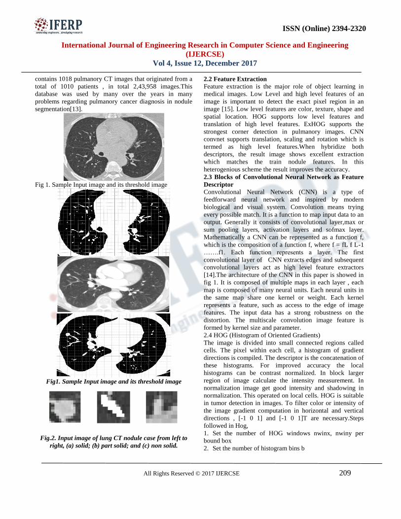
ISSN (Online) 2394-2320
International Journal of Engineering Research in Computer Science and Engineering
(IJERCSE)
Vol 4, Issue 12, December 2017
All Rights Reserved © 2017 IJERCSE 209
contains 1018 pulmanory CT images that originated from a
total of 1010 patients , in total 2,43,958 images.This
database was used by many over the years in many
problems regarding pulmanory cancer diagnosis in nodule
segmentation[13].
Fig 1. Sample Input image and its threshold image
Fig1. Sample Input image and its threshold image
Fig.2. Input image of lung CT nodule case from left to
right, (a) solid; (b) part solid; and (c) non solid.
2.2 Feature Extraction
Feature extraction is the major role of object learning in
medical images. Low Level and high level features of an
image is important to detect the exact pixel region in an
image [15]. Low level features are color, texture, shape and
spatial location. HOG supports low level features and
translation of high level features. ExHOG supports the
strongest corner detection in pulmanory images. CNN
convnet supports translation, scaling and rotation which is
termed as high level features.When hybridize both
descriptors, the result image shows excellent extraction
which matches the train nodule features. In this
heterogenious scheme the result improves the accuracy.
2.3 Blocks of Convolutional Neural Network as Feature
Descriptor
Convolutional Neural Network (CNN) is a type of
feedforward neural network and inspired by modern
biological and visual system. Convolution means trying
every possible match. It is a function to map input data to an
output. Generally it consists of convolutional layer,max or
sum pooling layers, activation layers and sofmax layer.
Mathematically a CNN can be represented as a function f,
which is the composition of a function f, where f = fL f L-1
…….f1. Each function represents a layer. The first
convolutional layer of CNN extracts edges and subsequent
convolutional layers act as high level feature extractors
[14].The architecture of the CNN in this paper is showed in
fig 1. It is composed of multiple maps in each layer , each
map is composed of many neural units. Each neural units in
the same map share one kernel or weight. Each kernel
represents a feature, such as access to the edge of image
features. The input data has a strong robustness on the
distortion. The multiscale convolution image feature is
formed by kernel size and parameter.
2.4 HOG (Histogram of Oriented Gradients)
The image is divided into small connected regions called
cells. The pixel within each cell, a histogram of gradient
directions is compiled. The descriptor is the concatenation of
these histograms. For improved accuracy the local
histograms can be contrast normalized. In block larger
region of image calculate the intensity measurement. In
normalization image get good intensity and shadowing in
normalization. This operated on local cells. HOG is suitable
in tumor detection in images. To filter color or intensity of
the image gradient computation in horizontal and vertical
directions , [-1 0 1] and [-1 0 1]T are necessary.Steps
followed in Hog,
1. Set the number of HOG windows nwinx, nwiny per
bound box
2. Set the number of histogram bins b
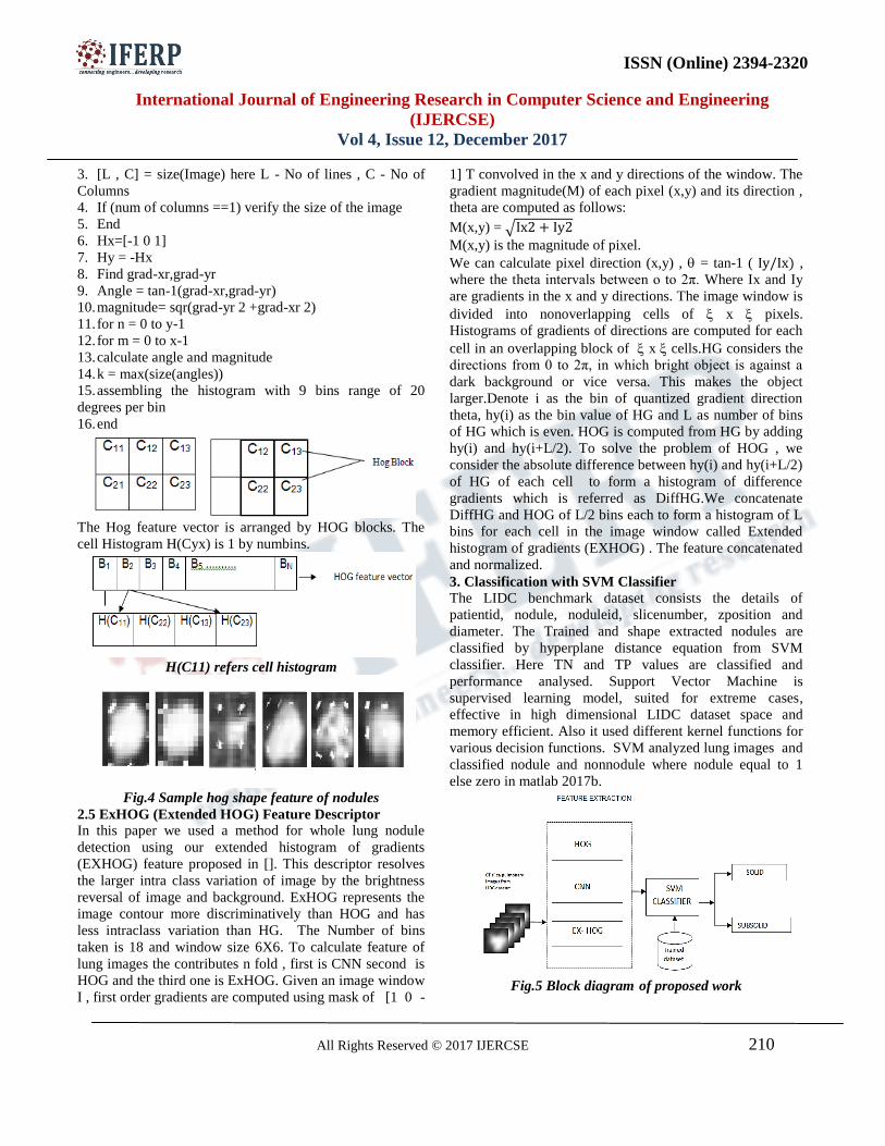
ISSN (Online) 2394-2320
International Journal of Engineering Research in Computer Science and Engineering
(IJERCSE)
Vol 4, Issue 12, December 2017
All Rights Reserved © 2017 IJERCSE 210
3. [L , C] = size(Image) here L - No of lines , C - No of
Columns
4. If (num of columns ==1) verify the size of the image
5. End
6. Hx=[-1 0 1]
7. Hy = -Hx
8. Find grad-xr,grad-yr
9. Angle = tan-1(grad-xr,grad-yr)
10. magnitude= sqr(grad-yr 2 +grad-xr 2)
11. for n = 0 to y-1
12. for m = 0 to x-1
13. calculate angle and magnitude
14. k = max(size(angles))
15. assembling the histogram with 9 bins range of 20
degrees per bin
16. end
The Hog feature vector is arranged by HOG blocks. The
cell Histogram H(Cyx) is 1 by numbins.
H(C11) refers cell histogram
Fig.4 Sample hog shape feature of nodules
2.5 ExHOG (Extended HOG) Feature Descriptor
In this paper we used a method for whole lung nodule
detection using our extended histogram of gradients
(EXHOG) feature proposed in []. This descriptor resolves
the larger intra class variation of image by the brightness
reversal of image and background. ExHOG represents the
image contour more discriminatively than HOG and has
less intraclass variation than HG. The Number of bins
taken is 18 and window size 6X6. To calculate feature of
lung images the contributes n fold , first is CNN second is
HOG and the third one is ExHOG. Given an image window
I , first order gradients are computed using mask of [1 0 -
1] T convolved in the x and y directions of the window. The
gradient magnitude(M) of each pixel (x,y) and its direction ,
theta are computed as follows:
M(x,y) = √
M(x,y) is the magnitude of pixel.
We can calculate pixel direction (x,y) , = tan-1 ( ,
where the theta intervals between o to 2π. Where Ix and Iy
are gradients in the x and y directions. The image window is
divided into nonoverlapping cells of x pixels.
Histograms of gradients of directions are computed for each
cell in an overlapping block of x cells.HG considers the
directions from 0 to 2π, in which bright object is against a
dark background or vice versa. This makes the object
larger.Denote i as the bin of quantized gradient direction
theta, hy(i) as the bin value of HG and L as number of bins
of HG which is even. HOG is computed from HG by adding
hy(i) and hy(i+L/2). To solve the problem of HOG , we
consider the absolute difference between hy(i) and hy(i+L/2)
of HG of each cell to form a histogram of difference
gradients which is referred as DiffHG.We concatenate
DiffHG and HOG of L/2 bins each to form a histogram of L
bins for each cell in the image window called Extended
histogram of gradients (EXHOG) . The feature concatenated
and normalized.
3. Classification with SVM Classifier The LIDC benchmark dataset consists the details of
patientid, nodule, noduleid, slicenumber, zposition and
diameter. The Trained and shape extracted nodules are
classified by hyperplane distance equation from SVM
classifier. Here TN and TP values are classified and
performance analysed. Support Vector Machine is
supervised learning model, suited for extreme cases,
effective in high dimensional LIDC dataset space and
memory efficient. Also it used different kernel functions for
various decision functions. SVM analyzed lung images and
classified nodule and nonnodule where nodule equal to 1
else zero in matlab 2017b.
Fig.5 Block diagram of proposed work
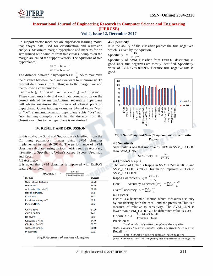
ISSN (Online) 2394-2320
International Journal of Engineering Research in Computer Science and Engineering
(IJERCSE)
Vol 4, Issue 12, December 2017
All Rights Reserved © 2017 IJERCSE 211
In support vector machines are supervised learning model
that anayze data used for classification and regression
analysis. Maximum margin hyperplane and margins for an
svm trained with samples from two classes. Samples on the
margin are called the support vectors. The equations of two
hyperplanes,
The distance between 2 hyperplanes is
. So to maximize
the distance between the planes we want to minimize . To
prevent data points from falling in to the margin, we add
the following constraint for i,
if yi =1 or if yi =-1
These constraints state that each data point must lie on the
correct side of the margin.Optimal separating hyperplane
will obtain maximize the distance of closest point to
hyperplane.. Given training examples labeled either “yes”
or “no”, a maximum-margin hyperplane splits “yes” and
“no” training examples, such that the distance from the
closest examples to the hyperplane is maximized.
IV. RESULT AND DISCUSSION
In this study, the Solid and Subsolid are classified from the
CT lung pulmanory images using SVM classifier
implemented in matlab 2017b. The performance of SVM
classifier calculated using various metrics such as Accuracy
, Sensitivity, Specificity, Cohen’s Kappa, Fscore , Precision
and Recall.
4.1 Accuracy
It is noted that SVM classifier is improved with ExHOG
feature descriptor.
Accuracy =
Fig.6 Accuracy of various classifiers
4.2 Specificity
It is the ability of the classifier predict the true negatives
which is given by the equation.
Specificity =
Specificity of SVM classifier from ExHOG descriptor is
good since true negatives are mostly identified. Specificity
value of ExHOG is 80.09%. Because true negative rate is
good.
Fig.7 Sensitivity and Specificity comparison with other
Papers
4.3 Sensitivity
Sensitivity is one that improve by .01% in SVM_EXHOG
than SVM_CNN.
Sensitivity =
4.4 Cohen’s Kappa
The value of Cohen’s Kappa in SVM_CNN is 58.36 and
SVM_EXHOG is 78.71.This metric improves 20.35% in
SVM_EXHOG%.
Kappa Coefficient (K) =
Here Accuracy Expected (Pe) = ∑
Overall accuracy P0 = ∑
4.5 FScore
Fscore is a benchmark metric, which measures accuracy
by considering both the recall and the precision.This is a
measure of relative to sensitivity. The SVM_CNN is
lower than SVM_EXHOG. The difference value is 4.39.
F Score = 2 X
Precision =
(
Recall =
(

ISSN (Online) 2394-2320
International Journal of Engineering Research in Computer Science and Engineering
(IJERCSE)
Vol 4, Issue 12, December 2017
All Rights Reserved © 2017 IJERCSE 212
Where TP (cancer pixels) is true positive that counts
classified foreground pixels.
FP counts the background pixels incorrectly classified as
foreground.
FN counts false negative that counts foreground pixels
incorrectly classified as background.
TN counts correctly classified background pixels.
V. CONCLUSION
The Proposed feature descriptor Extented Hog method
with classifier SVM in deep learning shows an improved
accuracy and specificity, a reduced FPR with reduced
computation time.This SVM classifier classify the solid ,
part solid and non solid. The Challenge is to decrease the
false positive rate and the method should be generalized
with other medical images which leads to Content Based
Retrieval in web search machine.
REFERRENCE
[1] A. McWilliams, et al., "Probability of cancer in
pulmonary nodules detected on first screening CT," New
England Journal of Medicine, vol. 369, pp. 910-919, 2013.
[2] V. K. Patel, et al., "A practical algorithmic approach to
the diagnosis and management of solitary pulmonary
nodules: part 2: pretest probability and algorithm," Chest,
vol. 143, pp. 840-846, 2013.
[3] D. P. Naidich, et al., "Recommendations for the
management of subsolid pulmonary nodules detected at
CT: a statement from the Fleischner Society," Radiology,
vol. 266, pp. 304-317, 2013.
[4] M. K. Gould, et al., "Evaluation of individuals with
pulmonary nodules: When is it lung cancer?: Diagnosis and
management of lung cancer: American College of Chest
Physicians evidence-based clinical practice guidelines,"
Chest, vol. 143, p. e93S, 2013.
[5] J.Gu.Z.Wang, J.Kuen, L.Ma, A,Shahroudy, B.Shuai,
T.Liu, D.Wang, and G.Wang, “Recent advances in
convolutional neural networks”, arXiv preprint
arXiv:1512.07108, 2015.
[6]Qing Zeng Song,Lei Zhao et al,Using Deep Learning for
Classification of Lung Nodules on Computed Tomography
Images”,JHE,vol.2017
[7]Sihong Chen, Jing Qin,Xing Ji,”Automatic Scoring of
Multiple Semantic Attributes with Multi-task Feature
Leverage: A study on Pulmonary Nodules in CT
Images”,IEEE,2016
[8] N. Dalal and B. Triggs, "Histograms of oriented
gradients for human detection," in CVPR 2005. IEEE, 2005,
pp. 886-893.
[9]Jie-Zhi Cheng, DOng Ni, Yi Hong Chou,Jing Qin et al,
“Computer Aided Diagonosis with Deep Learning
Architecture : Applications to Breast Lesions in US Images
and Pulmonary Nodules in CT Scans,Scientific Reports
,DOI:10.1038/sre/24454
[10]Juan-Juan Zhao and Guohua Ji,“Cavitary nodule
segmentation in computed tomography images based on self
generating neural networks and particle swarm
optimization”,inderscience,2015
[11] Arnaud A, A. Setio,Franceco Ciompi et al,”Pulmonary
nodule detection in CT images : false positive reduction
using multi-view convolutional networks,IEEE,2015
[12] Armato,S.G.,The Lung image database consortium
(LIDC) and image database resource initiative (IDRI), a
completed reference database of lung nodules on CT scans,
Medical Physics,38,915-931
[13]Novo, Rouco,Mendonca and Campilho,”Reliable lung
segmentation methodology by including justaplueral
nodules”,2014
[14] HE Yang,Hengyong Yu,”Deep Learning for the
classification of lung nodules”,article,2016
[15]Alif Hayat M,2015,Classifiction of membrane protein
types using voting feature interval in combination with
Choo’s pseudo amino acid composition. Theory Biology
384, 78-83

A Reliable Computer Aided Lung Cancer Classification System
Using Curvelet Features and Ensemble Classifier S. Piramu Kailasam1, M. Mohammed Sathik2
1Research Scholar, Research and Development Centre, Bharathiar University, Coimbatore, India 2Principal, SathakathullahAppa College, Tirunelveli, India
Abstract- Lung cancer is one of the dreadful diseases, which shows greater mortality rates. The lifespan of the patients can be improved, when the disease is detected earlier. Due to the advancement of medical science, several screening equipments are presented to the society. Computed Tomography (CT) is one of the prominent screening equipments for detecting lung cancer. It would be beneficial for the medical expert, when some reliable computer based assistance is rendered. Taking this into account, this article proposes a computer aided classification system for lung cancer detection by dividing the complete work into four phases. Initially, the contrast of the CT lung images are improved by Adaptive Histogram Equalization (AHE) and the image segmentation is carried out by Kernelized Fuzzy C Means (KFCM). The curvelet features are extracted from the segmented CT image and the ensemble classifier is applied over it. This way of benign and malignant classification results in reliable and accurate results. The performance of the proposed approach is evaluated with respect to accuracy, sensitivity, specificity and time consumption. The proposed classification approach shows better results, when compared to the existing approaches.
Keywords – Lung cancer, pre-processing, CT image, segmentation, ensemble classification.
1. Introduction Lung cancer is the fourth commonly occurring cancer next to breast, cervical and oral cavity cancer. Lung cancer is observed more in men rather than women, as per the medical reports. This dreadful disease is observed as the second and sixth mostly occurring cancer in men and women respectively [1]. The mortality rates with respect to lung cancer are improving every year. The main reason for the increased death rates is the ignorance and negligence of periodical health checkups. Early detection of any cancerous growth supports in increasing the lifespan of the patient. Due to the advancement of medical science and computer technology, computer based diagnostic systems come into picture. As the diagnostic systems assist the physician to make a decision, the reliability of the system is very important. The system is said to be reliable when the accuracy rates are reasonable. However, achieving better accuracy rates is a challenging task, as the images contain several unnecessary details. In spite of the presence of numerous lung cancer detection systems, there is a constant demand for a reliable system. Taking this challenge into consideration, this work attempts to propose a novel computer based diagnostic system for lung cancer detection by incorporating advanced image processing techniques over Computed Tomography (CT) images. The entire work is decomposed and organised into four important phases, which are CT image pre-processing,
segmentation, feature extraction and classification. The image pre-processing phase makes the CT images fitter for the forthcoming processes. Usually, the pre-processing phase attempts to enhance the quality of image by incorporating the noise removal or the contrast enhancement procedure and so on. The segmentation phase focuses on extracting the regions of interest from the whole image, such that the segmented regions alone are processed. The efficiency of the classification system improves, when specific regions of CT images are focussed. The features of the segmented regions are extracted, which are rich enough for the classifiers to detect the abnormalities being present in the CT images. The rest of this paper is organized as follows. A short review of the state-of-the-art literature with respect to lung cancer detection is presented in section 2. Section 3 presents the proposed lung cancer detection approach in a detailed manner. The performance of the proposed approach is analysed by executing several comparative analysis in section 4. The concluding points of this article are summed up in section 5. 2. Review of Literature The purpose of this section is to review the recent literature with respect to lung cancer detection systems. Several image processing techniques for the detection of lung cancer by using CT images are reviewed in [1]. The lung cancer detection is carried out by splitting the review in different aspects such as pre-processing, nodule segmentation and segmentation. The recent trends in lung nodule detection are presented in [2]. Additionally, the performance of the recent lung nodule detection techniques is compared and presented. In [3], a lung cancer classification system is proposed on the basis of wavelet recurrent neural network. This work employs wavelet to remove the noise from the input image and recurrent neural network is utilized for classification. However, this work cannot achieve better specificity rates and this implies that the false positive rates of the work are greater. A lung cancer detection technique, which is based on Local Energy based Shape Histogram (LESH) and machine learning techniques is introduced in [4]. Initially, this work pre-processes the CT images by Contrast Limited Adaptive Histogram Equalization (CLAHE) and the LESH features are extracted. A new lung cancer detection technique based on Mumford-Shah algorithm is proposed in [5]. This work removes the Gaussian noise by applying sigma filter and the regions of interest are segmented by otsu’sthresholding and mumford-shah model is applied. The texture features are extracted from the extracted regions by spectral texture extraction technique and the classification is done by multi-level slice classifier. An automatic lung nodule segmentation and classification technique is proposed in [6]. The areas of interest alone are extracted by means of priory
International Journal of Pure and Applied MathematicsVolume 117 No. 22 2017, 275-278ISSN: 1311-8080 (printed version); ISSN: 1314-3395 (on-line version)url: http://www.ijpam.euSpecial Issue ijpam.eu
275

information and Hounsfield Units. SVM is employed for achieving the task of classification. The results of this work can still be improved in terms of sensitivity and specificity. Motivated by these existing research works, this paper aims to present a reliable lung cancer detection algorithm, which can prove better sensitivity and specificity rates with minimal time complexity. The following section elaborates the proposed approach along with the overview of the work. 3. Proposed Lung Cancer Detection Approach The proposed lung cancer detection approach is based on several phases and all the involved phases are explained one after the other. A. CT Image Pre-processing by AHE Most of the medical images suffer from poor contrast issues and so the details of the images cannot be distinguished easily. At this juncture, the role of contrast enhancement algorithm comes into picture. The CT images are pre-processed by employing the AHE technique and the major reason for the exploitation of AHE is that this technique computes several histograms by considering separate areas of the CT image. This means that the contrast of every particular area of the image is enhanced. The computed histogram is adaptive, which ensures the balanced distribution of values. The AHE technique improves the edges and the local contrast of the CT image. Some of the sample pre-processed images are presented in figure 1.
Fig.1. (a) to (d) are input images (a1) to (d1) are the contrast
enhanced images Consider a CT image with pixels and is applied with the contrast enhancement process. The AHE processes each and every pixel and alters by considering the intensity immediate neighbourhood pixels. Unlike standard HE technique, AHE processes the regions of an image separately. This results in the contrast enhancement of each and every region, which in turn enhances the contrast of a complete image. B. KFCM based CT Image Segmentation This phase aims to segment or divide the CT image into several segments, such that each segment can be focussed with utmost care. This idea conserves time and computational power of the system. Hence, the process of segmentation renders several benefits to the classification system. FCM is one of the famous segmentation algorithms, which groups the pixels that show similar characteristic features. The input of the standard FCM algorithm is the image along with the total count of clusters. In order to improve the capability of clustering, this work launches a kernel function that can deal with noise as well. This work employs the Gaussian Radial Basis Function (GRBF) kernel and the kernel function is represented in the feature space as follows. ( ) ⟨ ( ) ( )⟩ (1) In the above equation, ⟨ ( ) ( )⟩ is the inner product. The GRBF kernel is denoted as
( ) ( || ||
) (2)
The objective function of the KFCM is presented as follows.
∑ ∑
|| ( ) ( )||
(3)
In the above equation, and are the total count of clusters and data points respectively. is the membership of the pixel in
the cluster and is the degree of fuzziness. indicates the non-linear mapping implicitly.
|| ( ) ( )|| ( ( ) ( ))
( ( ) ( )) (4)
Based on this equation, the objective function is modified as follows.
∑ ∑
( ( )) (5)
Where
( ( ))
( )
∑ ( ( ))
( )
(6)
∑
( )
∑ ( )
(7)
C. Feature Extraction by Curvelet Curvelet is a multidimensional and multiresolutional analytic tool, which is proposed by Candes and Donoho in the year 2000 [7]. The curvelets are simple and are easy to implement. Additionally, curvelets are faster with minimal redundancy. Initially, Fast Fourier Transform (FFT) is applied over the input image. The obtained fourier frequency plane is sliced into several wedges, which results in circular and angular slices. The circular slices decompose an image into several scales and the angular slices divide the images in different angles. Hence, all the wedges conform to a specific angle and scale. When the Inverse FFT (IFFT) is applied over a wedge, the curvelet coefficients can be obtained for a particular scale and angle. Additionally, the curvelets can handle the edge discontinuities in a better way. The CT images of lungs are considered in three different scales and the GLCM coefficients are extracted. GLCM features are effective in determining the spatial relationship between the pixels. The GLCM can be represented as a square matrix , where is the total number of gray levels being available in an image. All the entities being present in the GLCM is the approximation of probability of intensity between two pixels.
The ( ) entity of the GLCM matrix is formed when a pixel with coordinate ( ) has a gray level and then the pixel ( ) is found with the intensity . The
and are computed by considering different scales and angles. The features are computed by performing weight operation upon every entity of the matrix and the weighted values are added. The features being utilized by this work are energy, contrast, correlation, homogeneity, autocorrelation, dissimilarity and inertia. The co-occurrence is computed in three different angles such as 0, 45 and 90 degrees. D. Ensemble Classification When it comes to supervised learning, the classifiers are given knowledge with the features with which the classification is done. Normally, the process of classification requires prior knowledge about the dataset being utilised. The entire process of classification is achieved by two major phases namely training and testing. In the training phase, the classifier is imparted knowledge by means of the extracted features. By this way, the classifier equips itself in differentiating the objects. The classification problem can be a binary or multiclass problem. The binary classification system involves only two classes, whereas the multiclass problem has several classes involved in it. This work employs ensemble classifier, as the result of a single classifier may introduce false positives or false negatives. In order to ensure reliability, this work employs k-NN, SVM and ELM and the final decision is taken by performing majority vote computation. The final classification results of the k-NN, SVM and ELM are obtained and the dominating result is found out. As three different classifiers are utilized, eight different scenarios may
International Journal of Pure and Applied Mathematics Special Issue
276

occur. For instance, when two or three classifiers produce the same result, then that result is considered as dominating and the same result is declared as final. As this work does not rely on a single classifier to classify between the classes, the reliability of the system is improved. Additionally, in order to reduce time and computational complexity, this work exploits efficient classifiers. The false positive and false negative rates are considerably reduced, which in turn improves the sensitivity and specificity rates. The performance of the proposed approach is analysed in the following section. 4. Results and Discussion The functionality of the proposed approach is evaluated by implementing this work in Matlab version 8.1, on a stand alone computer with 8 GB RAM. The CT images are collected from different laboratories to carry out this research. The tailored dataset contains an image set of 100, which includes 37 and 63 benign and malignant images respectively. The initial round of comparative analysis justifies the choice of the incorporated techniques such as AHE, KFCM, curvelet features and ensemble classification. In the second round, the comparative analysis literally compares performance of the proposed classification approach with the existing literature proposed in LESH + CC [4], Mumford-Shah algorithm [5], apriori + SVM [6], in terms of classification accuracy, sensitivity, specificity and time consumption.
Fig 2. Performance analysis
The reason for the better performance of the proposed approach is that all the techniques involved in this work operate by themselves without any manual setting. Besides this, the better pre-processed and segmented results affect the quality of the classification process. When the initial image processing activities are optimal, obviously the outcome of the system is efficient. Hence, a better classification approach to distinguish between malignant and benign tumour in the lung CT scans is presented. The experimental results of the comparative results are presented in table.1.
Table.1 Performance analysis in terms of accuracy, sensitivity, specificity and time consumption
The experimental results of the proposed approach justify the choice of the techniques that are incorporated in it. The second to fourth columns of the table signifies the comparative technique for pre-processing, segmentation and feature extraction respectively. The columns five to seven indicates the performance
of the classifier being employed alone. Finally, the results of the proposed approach are presented. The proposed approach shows maximum accuracy, sensitivity and specificity, however the time consumption is a bit greater than ELM. Yet the time consumption is reasonable, as the results of the proposed approach performs ensemble classification and does not based on a single classifier. The attained time consumption is tolerable, as the degree of sensitivity and specificity are greater.
5. Conclusion This article presents a reliable computer aided lung cancer classification system based on curvelet features and ensemble classifier. The proposed classification approach is applied over the pre-processed and segmented images, which is accomplished by AHE and KFCM respectively. The features of the segmented regions of the image are extracted by means of curvelet, which is faster with high discrimination ability. The ensemble classifier which is formed by k-NN, SVM and ELM is proposed and the decisions of all the classifiers are obtained. The dominating result is chosen as the final decision and the performance of this work is tested against three different existing techniques. The proposed classification approach serves better in terms of accuracy, sensitivity and specificity rates with minimal time consumption. In future, this work is planned to be extended by including feature normalization and selection techniques. References [1] G. Niranjana ; M. Ponnavaikko, "A Review on Image
Processing Methods in Detecting Lung Cancer Using CT Images", International Conference on Technical Advancements in Computers and Communications, 10-11 April, Melmaruvathur, India, 2017.
[2] RabiaNaseem ; KhurramSaleemAlimgeer ; Tariq Bashir, "Recent trends in Computer Aided diagnosis of lung nodules in thorax CT scans", International Conference on Innovations in Electrical Engineering and Computational Technologies, 5-7 April, Karachi, Pakistan, 2017.
[3] DeviNurtiyasari ; DediRosadi ; Abdurakhman, "The application of Wavelet Recurrent Neural Network for lung cancer classification", International Conference on Science and Technology - Computer, 11-12 July, Yogyakarta, Indonesia, 2017.
[4] SummrinaKanwalWajid ; Amir Hussain ; Kaizhu Huang ; WadiiBoulila, "Lung cancer detection using Local Energy-based Shape Histogram (LESH) feature extraction and cognitive machine learning techniques", International Conference on Cognitive Informatics & Cognitive Computing, 22-23 Aug, CA, USA, 2016.
[5] R. Janudhivya ; S. Gomathi ; P. MadhuMathi ; J. Seetha, "A new approach for lung cancer cell detection using Mumford-shah algorithm", International Conference on Communication and Signal Processing, 6-8 Apr, Melmaruvathur, India, 2016.
[6] ElmarRendon-Gonzalez ; VolodymyrPonomaryov, "Automatic Lung nodule segmentation and classification in CT images based on SVM", International Kharkiv Symposium on Physics and Engineering of Microwaves, Millimeter and Submillimeter Waves, 20-24 June, Kharkiv, Ukraine, 2016.
*7+ Candes, E. J. &Donoho, D. L. (2000). “Curvelets—A surprisingly effective non-adaptiverepresentation for objects with Edges”, Vanderbilt University Press, Nashville, TN, 2000.
International Journal of Pure and Applied Mathematics Special Issue
277

278

Sadakath: A Research Bulletin
Sadakath: A Research Bulletin
Classification of Solitary pulmonary Nodule/Blob Images Using
Improved Local Binary Pattern [Z⊕ŻLBP]
S.Piramu Kailasam1, Dr.M.Mohamed Sathik2
Abstract
The Solitary Pulmonary Nodule(SPN) in chest radiographs of 3DCT at
risk population is an alert signal to lung cancer. In this paper, an improved
feature vector named Z with Ż Local Binary Pattern [Z⊕ŻLBP] is proposed
for extracting solitary pulmonary blob image features powerfully. The goal is
to reduce Local Binary Pattern (LBP) complexity by reducing the size of the
feature vector. In the proposed work by dividing the vicinity pixels in to non-
overlapped groups of Z and Ż (Tilted Z) further texture features of pulmonary
images are extracted for feature extraction. The Single Classifier KNN has
been used with distance metric for classification purpose. Performance
Evaluation Metric Accuracy and F-measure are used to measure the proposed
system.
Keywords: Classification, Pulmonary Image, Feature Extraction, Active
Contour, KNN Classifier
Introduction
Pulmonary images are very much important to detect lung diseases using CTimaging modality for the assessment of pulmonary blobs which is Region of Interest. Thefeature types of the pulmonary bolb(ROI) in CT images are important cues for themalignancy prediction [1-2], diagnosis and advance management [3-4].The texturefeatures of blob solidity and semantic morphology feature of speculation are critical todifferentiate of pulmonary blobs region and other subtypes. Meanwhile other semanticfeatures calcification pattern, roundedness, margin clearness are shown to be helpful forthe evaluation of blob classification. The region of interest may be found in bronchialtubes or outside of bronchial tube. If the blob<=3mm the detection of malignancy isdifficult. The determination of clinical characteristics may differ from patient to patientand also depends on experience of the observer. Computer aided diagnosis is an assistivesoftware package to provide computational diagnostic references for the clinical imagereading and decision making support. The histogram features for the high level textureanalysis helped to extract blob or blob feature. Ciompi et al [5] developed the bag offrequencies descriptor that can successfully distinguish 51 speculated blobs from theother 204 non-speculated blobs. However, the mapping is from the low level imagefeatures toward the high level semantic features in the domain of clinical terms is notstraight forward task This semantic feature assessment maybe useful for clinical analysis.The Lung Image Database Consortium (LIDC) dataset for its rich annotation databasesupports the training and testing CAD scheme[6-7]. The blobs diameters larger than3mm are further rated by radiologist referred with semantic features of ”subtlety”,
1Research Scholar, Bharathiar University, Coimbatore.2Principal, Sadakathullah Appa College, Tirunelveli.

2 S.Piramu Kailasam, Dr.M.Mohamed Sathik
Vol. V, Feb. 2018 SPECIAL ISSUE ISSN 2347-7644
”calcification”, ”spericity”, ”margin”, ”speculation”, ”texture”, ”lobulation”, ”internalstructure” and “malignancy”[8].
Absorption and scattering of illumination rays are the two major issues that causereduced quality of images. Several methods have been proposed to enhance the quality ofthe pulmonary images. Histogram equalization technique, Contrast stretching methodscapable to enhance the image quality. Contrast Limited Adaptive Histogram Equlization(CLAHE) has been applied to improve the image contrast. Otsu’s adaptive thresholdingmethod form image segmentation has been effective for many applications[9]. Thisprovides bright backgrounds for images. Various thresholding techniques such as Local,Global and Multilevel thresholding have been applied for the segmentation of pulmonarybolb images. The slice thickness of the LIDC CT Scans ranges from 1.25mm to3mm[10,11]. The texture feature descriptor that has been widely used for imageclassification is Local Binary Pattern. Pican et al. have used GLCM’s twenty four typesfeatures for extraction and for each image suitable features have to be chosen forextraction. Hence there is a need of efficient feature descriptor for classification process.In past years Neural Network is performed for classification results time consuming. K-Nearest Neighbour as classifier with Euclidean distance used to classify blobs.Padmavathi et al[15] have classified images using probalisitic neural network whichgives better results than SIFT algorithm with three classes of dataset. Eduardo et al haveclassified images using nine machine learning algorithms such as: Decision Trees,Random Forest, Extremely Randomised Trees , Boosting, Gradient Boosted Trees, NormalBayes Classifier, Expectation Maximization, NN and SVM. Bhuvaneswari.P et al[16] haveclassified coral and textures using KNN by considering K=1 and the accuracy reported as90.35%.
The main tasks in this paper are in 4 steps as follows:
1. The features of blobs are enhanced from LIDC dataset.
2. The dimension of the LBP feature vector is condensed by novel feature descriptor Z
with Tilted Z Local Binary Pattern [Z⊕ŻLBP].
3. The Complication is reasonably reduced and accuracy is raised from existing CenterSymmetric Local Binary Pattern and Orthogonal Combination of Local Binary Pattern.
4. KNN with distance metric have been used.
Proposed Work
To find artfaceted of image, Adaptive Histogram Equalization (AHE) methodapplied to homogeneous regions of the pulmonary blob. This blur problem has beenovercome by Contrast Limited Adaptive Histogram Equalization (CLAHE) method. Itavoids the magnification of noise that might limit the artifactuals.
Figure 1: Pulmonary image

Classification of Solitary pulmonary Nodule/Blob Images Using Improved Local Binary
Pattern [Z⊕ŻLBP] 3
Sadakath: A Research Bulletin
Figure2: Bolb detection in a pulmonary image
(a) Lung Bolb in Segmented in red area, (b)Target Bolb in bronchial,
(c) Path to reach Bolb
Image segmentation, edge based and region based active contours are available.Edge based segmentation depends on image gradient that acts as an edge detector toinitiate boundaries of sub regions by outlining contours of detected boundaries. Regionbased active contour technique is similar to region based segmentation depends onstatistical information of image intensity inside each subset. Compared to other methodsactive contour method deliver continuous boundaries of sub regions and merge multiplecontours into one contour. It works well for both global and local cluster regions.
Figure 3: Sample trained data
Texture features are important useful information for discrimination purposes.
The [Z⊕ŻLBP] reduces the dimensionality of the original LBP histogram while
preserving its discriminative power.
Figure 4: Block Diagram of Proposed Method
The proposed Feature Descriptor [Z ⊕Ż LBP]
The Computed Tomography LIDC[11] dataset is trained with each five slices. Thefive slices taken as p-2,p-1,p,p+1, p+2, where p - present slice and vice versa. Each 3dsegmented[9,12] bolb LBP texture value calculated for every five slices and it applied toall trained data. The trained class checked with tested data class. In CS-LBP(CentreSymmetric Local Binary Pattern) , the information of the centre pixel is not considered .When neighbours increase, CS-LBP’s feature vector size also increases. In OC-LBP(Orthogonal Combination of Local Binary Pattern) , diagonal information is not

4 S.Piramu Kailasam, Dr.M.Mohamed Sathik
Vol. V, Feb. 2018 SPECIAL ISSUE ISSN 2347-7644
considered. But in [Z⊕ŻLBP] diagonal information is also considered by Z and Ż groups.
[Z⊕ŻLBP] operator is proposed to reduce the dimension of feature vector and to
increase the classification accuracy. According to [Z⊕ŻLBP, a 3 x 3 neighbour pixel is
viewed as two non overlapping Z and Ż groups. Separately Z and Ż feature vector groupformation is performed and finally they concatenated.
Figure 5: Block Bk of matrix 3 x 3 with the centre pixel Xij and its neighbour pixels
Figure 6: Illustration of [Z⊕ŻLBP] template as z neighbours in 3 x 3 region.
Figure 7: Ż neighbours of 3 x 3 neighbourhood region.
(a) (b)
Figure8: Neighbours considered for [Z⊕ŻLBP] combinations (a) Z neighbours
(b) Ż neighbours are highlighted
In pulmonary image, take Block Bk, where 1≤k≤N and N is the total number ofblocks in an image. Let Xij be the centre pixel of a 3 x 3 block Bk as shown in the Fig.5.Among the eight neighbours four are considered as the Z neighbours and the other four
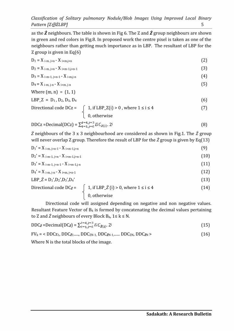
Classification of Solitary pulmonary Nodule/Blob Images Using Improved Local Binary
Pattern [Z⊕ŻLBP] 5
Sadakath: A Research Bulletin
as the Ż neighbours. The table is shown in Fig 6. The Z and Ż group neighbours are shownin green and red colors in Fig.8. In proposed work the centre pixel is taken as one of theneighbours rather than getting much importance as in LBP. The resultant of LBP for theZ group is given in Eq(6)
D1 = X i-m, j+n - X i+m,j+n (2)
D2 = X i-m, j+n - X i+m-1,j+n-1 (3)
D3 = X i-m-1, j+n-1 - X i-m,j-n (4)
D4 = X i-m, j-n - X i+m, j-n (5)
Where (m, n) = (1, 1)
LBP_Z = D1 , D2, D3, D4 (6)
Directional code DCz = 1, if LBP_Z(i) > 0 , where 1 ≤ i ≤ 4 (7)
0, otherwise
DDCz =Decimal(DCz) = ∑ ( ).,, 2j (8)
Ż neighbours of the 3 x 3 neighbourhood are considered as shown in Fig.1. The Ż groupwill never overlap Z group. Therefore the result of LBP for the Ż group is given by Eq(13)
D1’ = X i-m, j+n-1 - X i+m-1,j+n (9)
D2’ = X i-m-1, j+n - X i+m-1,j+n-1 (10)
D3’ = X i-m-1, j+n-1 - X i+m-1,j-n (11)
D4’ = X i-m, j-n - X i+m, j+n-1 (12)
LBP_Ż = D1’,D2’,D3’,D4’ (13)
Directional code DCŻ = 1, if LBP_Ż (i) > 0, where 1 ≤ i ≤ 4 (14)
0, otherwise
Directional code will assigned depending on negative and non negative values.Resultant Feature Vector of Bk is formed by concatenating the decimal values pertainingto Z and Ż neighbours of every Block Bk, 1≤ k ≤ N.
DDCŻ =Decimal(DCŻ) = ∑ Ż( ).,, 2j (15)
FVk = < DDCz1, DDCŻ1....., DDCZN-1, DDCŻN-1,...... DDCZN, DDCŻN > (16)
Where N is the total blocks of the image.

6 S.Piramu Kailasam, Dr.M.Mohamed Sathik
Vol. V, Feb. 2018 SPECIAL ISSUE ISSN 2347-7644
Algorithm: Texture feature Extraction using proposed feature vector
Input : Segmented 3D CT pulmonary image slices
Output : FV is termed as feature vector
Do for segmented CT slices (p-2,p-1,p,p+1,p+2) of every block Bk
Compute D for Z neighbour using Eq(2 ) to Eq(5)
LBP_Z value is calculated using eq(6)
Directional Code for DCZ is calculated using Eq (7)
DDCZ value is calculated using Eq(8)
Compute D’ for Ż neighbours using Eq.(9) and Eq(12)
LBP_Ż is calculated using Eq(13)
Directional Code for DC_Ż is calculated using Eq(14)
DDCŻ is calculated using Eq(15)
Resultant feature vector of [Z⊕ŻLBP] is calculated using Eq(16)
End
Store the values of feature vector for classification.
Figure 9: Algorithm of the proposed [Z⊕ŻLBP] operator for pulmonary images
K-Nearest Neighbour Classification
Classification is learning a function that maps a data item into one of severalpredefined classes. The classification accuracy Ai of an individual program depends onthe number of samples correctly classified. In pattern recognition K-Nearest Neighbouralgorithm is a non – parametric method for classification. K-NN is a type of instance –based learning. In KNN classification[13], the output is a class membership. Theproposed improved [Z⊻ŻLBP] operator with K-NN classification worked in matlab16a.
The classification method used is KNN classifier with various distance metrices. It findsthe correlation between quantitative, continuous variables. Small SPN imageclassification assessment is a risk task. The image is classified by a majority vote of its knearest neighbours. If u = (u1,u2,....un) and v = (v1,v2,....vn) then the Euclidean distancebetween the feature vectors u and v is given below.
(u1 - v1)2 + (u2 - v2)2+ ............+(un - vn)2
D(u,v) = (u − v ) + (u − v ) + . . . . . . . . . . . . +(u − v ) (17)
Where u and v are training and testing samples generated from the histograms of thefeatures.
The steps involved in a KNN algorithm,
Step 1: Start
Step 2: Initialize and define the parameter K
Step 3: Find the distance between the test sample and all the training samples
Step 4: Sort out the Distance

Classification of Solitary pulmonary Nodule/Blob Images Using Improved Local Binary
Pattern [Z⊕ŻLBP] 7
Sadakath: A Research Bulletin
Step 5: Take K-Nearest Neighbour value
Step 6: Apply simple majority of category
Step 7: End
The feature descriptor LBP has histogram formation value as 2N. But the proposedfeature descriptor histogram is 2 X N. Average time taken for LBP is 0.53secs. Theresultant average time taken by proposed is 0.38secs.
Quantitative Comparison
1. F-measure
F-measure is a standard metric, which measures the image classification andsegmentation accuracy by combining both precision and recall values.
F measure = 2 x (18)
where Precision = (19)
Recall = (20)
2. Overall Accuracy
The overall accuracy (OA) of the classified LIDC dataset is derived by the ratio ofthe number of correctly classified tested samples and the total number of tested samples.
Overall Accuracy (OA) = (21)
3. Cohen’s Kappa
The value of Cohen’s Kappa of LBP_KNN and [Z⊕ŻLBP] got same value as 74.14%.
Kappa Coefficient (K) = (22)
Wherena is number of agreements, ne is number of agreements due to chance and n isnumber of samples.
Figure10: Performance Metrics Analysis of LBP and [Z⊕ŻLBP] with KNN Classifier
0.9462 0.9317 0.9414
0.7414
0.9582 0.9417 0.9614
0.7414
0
0.5
1
Fscore Precision Recall kappa
LBP_KNN
Z ⊻ ŻLBP_KNN

8 S.Piramu Kailasam, Dr.M.Mohamed Sathik
Vol. V, Feb. 2018 SPECIAL ISSUE ISSN 2347-7644
Conclusion
The proposed [Z⊕ŻLBP] feature descriptor is best competent for SolitaryPulmonary Nodule/Blob images and texture datasets. This feature descriptor extractsmore detailed information by dropping the size of the feature vector bin size of 8. The F-measure, Precision, Recall and Kappa coefficient are compared with uniform pattern.Compared to the existing feature descriptors the proposed [Z⊕ŻLBP] with KNN classifierprovides an improvement of 3.5% on accuracy as 95.48%. In future shape features andother texture features of pulmonary images can be calculated for Content Based ImageRetrieval from Web Search Engine.
References
[1]. McWilliams , et al.,” Probability of cancer in pulmonary nodules detected on firstscreening CT”, New England Journal of Medicine, Vol,369,pp.910-919,2013
[2]. V.K.Patel et al;, “A Practical algorithmic approach to the diagnosis and managementof solitary pulmonary nodules part 2: pretest probability and algorithm”,Chest,vol143, pp 840-846, 2013
[3]. D.P.Naidich, et al., “ Recommendations for the management of subsolid pulmonarynodules detected at CT: a statement from the Fleischner society”, Radiology,vol266,2013
[4]. M.K.Gould et al., “Elevation of individuals with pulmonary nodules when is it lungcancer? Diagonosis and management of lung cancer American college of chestphysicians evidence based clinical practice guidelines” Chest, vol 143,2013
[5]. F.Ciompi, et al., “Bag of frequencies: A Descriptor of pulmonary nodules inComputed Tomography Images”, IEEE Transcactions on Medical Imaging, Vol 34,pp962-973,2015
[6]. S.G.Armato III,et al., “ The lung image database consortium(LIDC) and imagedatabase resource initiative (IDRI); a completed reference database of lung noduleson CT scans “, Medical Physics.vol 38,pp 915-931,2011
[7]. S.G.Armato III,et al., “ The lung image database consortium: Developing a resourcefor the medical imaging research community 1”, Radiology , vol 232,pp,739-748,2004.
[8]. Sihong Chen,Jing Qin,Xing Ji et al, Automatic Scoring of Multiple Semantic Attributeswith Multi-task Feature Leverage : A study on Pulmonary nodules in CTImages,IEEE,2016
[9]. Juan-Juan Zhao and Guohua Ji, “Cavitary nodule segmentation in computedtomography images based on self generating neural networks and particle swarmoptimization”,inderscience,2015
[10]. Arnaud A, A. Setio, Franceco Ciompi et al, ”Pulmonary nodule detection in CT images: false positive reduction using multi-view convolutional networks, IEEE,2015
[11]. Armato, S.G., The Lung image database consortium (LIDC) and image databaseresource initiative (IDRI), a completed reference database of lung nodules on CTscans, Medical Physics,38,915-931
Classification of Solitary pulmonary Nodule/Blob Images Using Improved Local Binary
Pattern [Z⊕ŻLBP] 9
Sadakath: A Research Bulletin
[12]. Novo, Rouco, Mendonca and Campilho, ” Reliable lung segmentation methodologyby including just a plueral nodules”,2014
[13]. Alif Hayat M, ”Classification of membrane protein types using voting feature intervalin combination with Choo’s pseudo amino acid composition. ”,Theory Biology384,78-83,2015
[14]. A.Sherley Alphone,Dejey Dharma,”Novel directional patterns and generalizedsupervised dimension reduction system(GSDES) for facial emotionrecognition”,JMTA,2017
[15]. Padmavathi et al, “Kernel Principal component analysis feature detection andclassification for under water images”,(CISP),2010
[16]. P.Bhuvaneswari,Dr.A.Brintha therese,”Detection of cancer in lung with KNNclassification using genetic algorithm”,Elsevier,2015

International Journal of Multidisciplinary Approach
and Studies ISSN NO:: 2348 – 537X
Volume 06, No.4, July – Aug 2019
Pag
e : 5
7
A Survey on Pulmonary CT Image Classification in Deep learning
Dr. M. Mohamed Sathik*, & S Piramu Kailasam**
Principal,Sadakathullah Appa College,Tirunelveli,India
Assistant Professor,Sadakathullah Appa College,Tirunelveli,India
ABSTRACT
Image Classification in deep learning is a recently developed Soft computing method to
classify image data with pixel information in a way that only hybrid technique can do better
access using the pixel data in the aspect of performance measures. Classification is used to
predict the unknown data. Deep learning is a cascade of nonlinear transformation in a
hierarchical model as well as convert feed forward deep architecture worked on any image
size.
Lung Cancer is one of the leading diseases in the world and increased in many countries. The
eight years overall survival rate is just 17%. Early to remove lung cancer surgically will
ensure the survival of the patient. Before surgery a doctor needs help of radiologists
suggestion. In digital era, fast CAD’s system plays a vital role in surgery. In this junction,
medical image analysis, image classification, image detection and diagnosis involved much
in past decades. Pre-processing and Segmentation are the preliminary basic works for binary
classification.
KEYWORDS: Image Pre-processing, Image Enhancement, Descriptor, Image
Classification
I . INTRODUCTION
The purpose of this section is to review the recent literature with respect to lung cancer
detection systems.
1.1 PreProcessing
Several image processing techniques for the detection of lung cancer by using CT images are
reviewed in (Niranja.G et al., 2017). The lung cancer detection is carried out by splitting the
review in different aspects such as pre-processing, nodule segmentation and segmentation.
The recent trends in lung nodule detection are presented in
(Rabia Naseem et al., 2017). Additionally, the performance of the recent lung nodule
detection techniques are compared and presented. In (Devi Nurtiyasari et al., 2017), a lung
cancer classification system is proposed on the basis of wavelet recurrent neural network. This
author employs wavelet to remove the noise from the input image and the recurrent neural
network is utilized for classification. However, this author could not achieve better specificity
rates and this implies that the false positive rates of the work are greater.
The lung cancer detection algorithm based on FCM and Bayesian classification is presented
in (Bhagyarekha.U et al., 2016). In this paper, FCM is applied to achieve segmentation and the
GLCM features are extracted. Based on the feature set, the Bayesian classifier is employed to
distinguish between the normal and cancer affected CT images. Yet, the results of this work

International Journal of Multidisciplinary Approach
and Studies ISSN NO:: 2348 – 537X
Volume 06, No.4, July – Aug 2019
Pag
e : 5
8
are not convincing in terms of sensitivity and specificity rates. In (Manasee KurKure et al.,
2016), a lung cancer detection technique that relies on genetic approach is proposed.
However, this work involves more time complexity and the number of connected objects
have been calculated by assigning 1 to inside and 0 to outside of the object that shows brain
MRI image based on threshold technique to improve the skull stripping performance (Nilesh
Bhaskarrao Bahadur et al., 2017).
1.2 Segmentation Techniques
Image segmentation by different methods was done by many people. Some of them are Local
entropy image segmentation (Ali Shojaee Bakhtiari et al., 2007; L.Goncalves, J.Novo, 2016),
Discrete cosine texture feature (Chi-man pun et al., 2010), parallel algorithm for grey scale
image (Harvey et al., 1996), Clustering of spatial patterns and watershed algorithm (Kai-Jian
et al., 2010), Medical image segmentation (Prasantha H.S. et al., 2010), Finite bivariate
doubly truncated Gaussian Mixture model (Rajkumar 2010), Random set of view of texture
(Ramana Reddy 2010), Sobel operator technique, Prewitt technique, Kiresh technique,
Laplacian technique, Canny technique, Roberts technique and Edge maximization Technique
(Salem Saleh 2010), Mathematical image processing (Sun hee kim 2010), Simple algorithm
for image denoising (Vijaya 2010), Iterative regularized likelihood learning algorithm (Zhiwu
Lu 2006), Automatic model selection and unsupervised image segmentation by Zhi Wu Lu
(2007), finite mixtures and entropy regularization by Zhi wu Lu (2008).
As described by the Sun Hee Kim the following steps are followed in image processing for
counting the number of mosquitoes in a room (1) The acquisition of the image. (2) The
extraction of the region of the mosquitoes. The intensity and the property of the location of
the mosquitoes considering the image. (3) Reduction of the image to smaller size to process
in matlab. The image processing is applied to separate the region of mosquitoes and
backgrounds. Then the smaller size is obtained by processing it in paint. (4) Use array editor
convert the image to values. The recognized mosquitoes by the method of the array editor
conversion from the matlab software. (5) Identify the cluster where mosquitoes are present.
The place where the mosquitoes are there shows lesser value because of darkness. Here the
raw figure converted into values that can be processed by computer algorithms. The
conversion of the figure to a smaller size is done and the image is converted to array editor
values (Harvey A et al., 1996).
In (Xia Li et al., 2017), an algorithm is proposed to detect the pulmonary nodules based on
cascade classifier. This work detects the pulmonary nodules and classifies them into normal
and benign. A learning method is based on cascade classifier and applied over the detected
pulmonary nodules. This work focuses more on accuracy rates, rather than on sensitivity and
specificity rates. A technique to detect lung nodules from a series of CT slices is presented in
(May Phu Paing, 2017). This work segments the lung nodules by applying Otsu‟s threshold
along with some morphological operations. The geometric, histogram and texture features are
extracted from the segmented nodules to carry out the process of classification. The
Multilayer Perceptron (MLP) is employed as a classifier and this work involves
computational overhead. In (S.Avinash et al., 2016), a Gabor filter and watershed
segmentation based lung cancer detection technique is proposed. The process of segmentation
is carried out by watershed segmentation approach and the Gabor features are extracted from
the CT images. This technique does not include the process of classification and it stops itself
with segmentation.

International Journal of Multidisciplinary Approach
and Studies ISSN NO:: 2348 – 537X
Volume 06, No.4, July – Aug 2019
Pag
e : 5
9
A large number of lung segmentation methods have been proposed. Among them,
bidirectional differential chain code combined with machine learning framework is able to
correctly include the just a pleura nodules into the lung tissue while minimizing over under
segmentation. This method is capable of identifying low-dose, concave/convex regions
(Shiwen Shen 2015). In the Hessian-based approach, 3D lung nodule has been segmented in
the multiscale process through the combination of Shape Index and Curvedness methods.
Image characteristics, Nodule position, nodule size, and nodule characteristics are included in
this approach. Eigenvalues are computed from the 3 x 3 Hessian Matrix (L.Conclaves et al.,
2016).
2 Feature Vectors
The feature types of the pulmonary nodule in CT images are important cues for the
malignancy prediction (A.McWilliams et al., 2013, V.K.Patel et al., 2013), diagnosis and
advanced management (D.P.Naidich et al., 2013, M.K.Gould et al., 2013). The texture features
of nodule solidity and semantic morphology feature of speculation are critical to
differentiating of pulmonary nodules and other subtypes. Meanwhile, other semantic features
like calcification pattern, roundedness and margin clearness are shown to be helpful for the
evaluation of nodule classification. The nodule may be found in bronchial tubes or outside of
the bronchial tube. If the nodule<=3mm the detection of malignancy is difficult. The
determination of clinical characteristics may differ from patient to patient and depends on the
experience of the observer.
Computer-aided diagnosis (Shiwen shen, Alex A.T.Bui et al., 2015) is an assistive software
package to provide computational diagnostic references for the clinical image reading and
decision making support. The histogram feature (Sherly Alphonse,
Dejey Dharma, 2016) for the high-level texture analysis helps to extract nodule feature. The
bag of frequencies descriptor is developed that can successfully distinguish 51 spiculated
nodules from the other 204 non-spiculated nodules (Ciompi et al., 2015). However, the
mapping from the low-level image features toward the high-level semantic features in the
domain of clinical terms is not a straightforward task. This semantic feature assessment
maybe useful for clinical analysis. The Lung Image Database Consortium (LIDC) dataset for
its rich annotation database supports the training and testing CAD scheme (S.G.ArmatoIII et
al., 2011).
Absorption and scattering of light rays are the two major issues that cause reduced quality of
images. Several methods have been proposed to enhance the quality of the pulmonary
images. Histogram equalization technique and Contrast stretching methods are capable of
enhancing the image quality. Contrast Limited Adaptive Histogram Equalization (CLAHE) has
been applied to improve the image contrast. Otsu‟s adaptive thresholding method form image
segmentation has been effective for many applications. This provides bright backgrounds for
images. Various thresholding techniques such as Local, Global and Multilevel thresholding
have been applied for the segmentation of pulmonary nodules images. The texture feature
descriptor that has been widely used for image classification is Local Binary Pattern. Pican et
al., have used GLCM‟s twenty-four types of features for extraction and for each image
suitable features have to be chosen for extraction. Hence there is a need for efficient feature
descriptor for the classification process. In past years Neural Network is performed for
classification. The process is time-consuming. K-Nearest Neighbour as a classifier with
Euclidean distance was used to classify nodules. Padmavathi et al., (2010) have classified

International Journal of Multidisciplinary Approach
and Studies ISSN NO:: 2348 – 537X
Volume 06, No.4, July – Aug 2019
Pag
e : 6
0
images using a probabilistic neural network which gives better results than SIFT algorithm
with three classes of the dataset. Eduardo et al., have classified images using nine machine
learning algorithms such as Decision Trees, Random Forest, Extremely Randomised Trees,
Boosting, Gradient Boosted Trees, Normal Bayes Classifier, Expectation Maximization, NN
and SVM. Bhuvaneswari.P et al., (2015) have classified coral and textures using KNN by
considering K=1 and the accuracy was reported as 90.35%.
In (K.Gopi et al., 2017), a technique based on Ek-means algorithm and Support Vector
Machine (SVM) is presented to recognize and classify a lung tumor. This work pre-processes
the CT images for removing the unwanted information by means of thresholding approach.
The Threshold value calculated by Zack‟s Algorithm in white blood cell segmentation by
F.Sadglian et al., 2009. The regions of interest alone are extracted and the Gray Level Co-
occurrence Matrix (GLCM) features are extracted. Gray level co-occurrence matrix texture
features of CT image of small solitary pulmonary nodules(Vishal K Patel,K Naik, 2015),
which can profit diagnosis lung cancer in earlier by five combined patient level features
inertia, entropy, correlation, difference-mean and sum-entropy (Huan Wang et al., 2010).
Finally, SVM is utilized to distinguish between the cancerous and non-cancerous areas. An
early lung cancer detection mechanism is proposed in (Rachid Sammouda et al., 2016), which
exploits Hopfield Neural Network classifier for extracting the lung areas from the CT images.
The edges of the lung region lobes are detected by bit planes and the diagnostic rules are
framed to detect the abnormality.
A lung cancer detection technique, which is based on Local Energy based Shape Histogram
(LESH) and machine learning technique are introduced .Initially, this work pre-processes the
CT images by Contrast Limited Adaptive Histogram Equalization (CLAHE) and the LESH
features are extracted. Machine learning algorithms such as Extreme Learning Machine
(ELM) and SVM are applied. This work is efficient but the computational overhead can still
be decreased by altering the feature extracting technique. Shape features (Ashis et al., 2016)
are easily extracted by HOG (Histogram of Oriented Gradients) feature descriptor (Chen J et al.,
2014). The other method which is extension of HOG detected whole human detection using
EXHOG (Extended Histogram of Gradients) feature descriptor (Amit et al., 2011). HOG
method always deals with 180-degree angle whereas EXHOG method considers 360 degrees.
A Variety of Shape-based, margin-based and texture-based features are analyzed to improve
the accuracy of classification. These results are evaluated in terms of area under the receiver-
operating-characteristic-curve in Ashis Kumar et al., (2016) paper. Nodules are categorized
with rank1, rank2, rank3, rank4 and rank5 with malignancy ratings solid, part-solid and Non-
solid. Based on 2D Shape-Based Features and 3D Shape-Based Features the Nodules
Features are extracted. Han et al., introduced 3D Haralick features. Fourteen Haralick
features (1973) were computed from each GLCM matrix. The maximum correlation
coefficient is not considered in our experiment, as it is computationally expensive (Han et al.,
2014). Several shapes based, margin based and texture based features are computed to
represent the pulmonary nodules.
A set of relevant features is determined for the efficient representation of nodules in the
feature space. Han et al., introduced 3D Haralick features considering nine directions which
provide better classification performance than five directions. The performance of
classification is evaluated in terms of area (A), under the receiver operating characteristic
curve (Ashis Kumar Dhara et al., 2016). Predicting membrane protein sequences in

International Journal of Multidisciplinary Approach
and Studies ISSN NO:: 2348 – 537X
Volume 06, No.4, July – Aug 2019
Pag
e : 6
1
imbalanced data set is often handled by a decision tree, AdaBoost, random and rotation
forest, SVM and naive Bayes classifiers. The random forest has good performance except for
classes with fewer samples (E.Siva Shankari et al., 2017). Local Binary Pattern is an
incredibly well-known texture feature descriptor (D.Jeyabharathi, Dejey 2016) that has been
used in many application such as facial recognition (Ani brown et al., 2017), texture
classification and coral image classification. Contrast Limited Adaptive Histogram
Equalization (CLAHE) (Ani brown et al., 2017) has been applied for coral images to improve
the image contrast and equalize the image histogram effectively.
The relational feature provides information about the relational and hierarchical structure of
the regions related to a single object or a group of objects. Neural Network classifiers and
SVM classifier
2.1 DCNN as Feature Vector
Eduardo et al., have used wavelet filters to extract texture feature from OpenCV library
(Shiela et al.,) and have determined the counts of corals by extracting texture features using
LBP descriptor because they use the information from eight directions around a pixel (Huan
Wang 2010). Deep feed-forward ANN analyses the visual imagery. Artificial Neural
Networks consist of a method of solving problems related to science through simple models
that mimic the human brain, including their behaviour. An ANN is armed by small modules
which simulate the operation of a neuron. In ANN with a minimum number of layers are
used. Because the dimension of ANN is very limited. Deep feed-forward ANN analyses the
visual imagery. The convolutional neural network has hundreds of hidden layers, using filters
can extract the data. When the target reaches the value no change in weight. In sentiment
classification, RNN network is highly preferable. Recurrent Neural Network uses the loop to
translate sequence to sequence. This happens by sequence to a single output. Neurons within
the same layer are not connected. So in RNN, the neurons in the layers are connected. RNN is
the best for Reinforcement learning. Imagenet is suitable for Visual recognition challenges.
Instead of autoencoder, we can use Conditional Random Field (CRF) model or deep
sequential model.
Handwritten digit recognition using backpropagation over a coalitional network makes a
good change. Alexnet, Zfnet, VGGnet, Googlenet, and MsresNet are the other Neural
models. CNN was introduced by Lecun et al., 1998, CNN allows multiple features to be
extracted at each hidden layer. Convolutional Neural Network is used to classify tumors seen
in lung cancer screening, have special properties such as spatial invariance and allows to
multiple feature extraction. The deep CNN has been shown widely that the accuracy of
prediction increases dramatically (Prajwal Rao et al., 2016). Lecun et al., have written a paper
that CNN has been shown to eliminate the necessity of handcrafted feature extractors in gradient-
based learning applied to document recognition (Lecun et al., 1998). Hence, multiple
characteristics can be extracted and the learning process assigns weights appropriately to
significant features. So automatically performing the difficult task of feature engineering in
hierarchically. AlexNet using binary classification gives challenging visual task in face
recognition.
Convolutional Neural Networks are alternative type of neural network. This method can be
useful to reduce variations in spectral and model correlations in signals. Speech signals
exhibit both properties, hence CNN's are more effective model for speech compared to Deep

International Journal of Multidisciplinary Approach
and Studies ISSN NO:: 2348 – 537X
Volume 06, No.4, July – Aug 2019
Pag
e : 6
2
Neural Networks. In prior the number of convolutional layers, filter size and pooling size
needed is decided. Secondly, investigate an appropriate number of hidden units and best
pooling strategy. Then find how to incorporate speaker-adapted features. Finally, give the
importance of sequence training for speech tasks. During Hessian free sequence training of
CNN's, using ReLU+dropout can be done the process (Prajwal Rao et al., 2016).
Convolutional Neural network recognizes face using a Self-Organizing Map (SOM) neural
network and a CNN. MatConvNet is an open source for the convolutional neural network. In
XNOR networks or Image Net, both the filters and the input to convolutional layers are
binary. The filters are approximated with binary values resulting in 32x memory savings.
The paper Arnaud A.A Setio et al., 2015 showed the multi-view ConvNet. This is very much
suited for false positive reduction and achieved good results for the nodule detection task of
lung CT images. CNN is an automated Preprocessing architecture so no need to do
preprocessing again. In Deep Learning (Qing zeng song, lei zhao, xing ke, 2017) images or
videos may profit from preprocessing, whose job may become much easier (Jodogne and
Piater, 2007, Legenstein et al., 2010, Cuccu et al., 2011). A dominant dictionary like texture
descriptor, texton is proposed as a feature (Beijbom et al., 2012). Deep learning has proved a
popular and powerful method in many medical imaging areas. In (QingZeng Song et al.,
2017) paper CNN, DNN, and SAE are designed for lung cancer calcification. The
experimental result achieved the best performance with accuracy among the three
architectures.
3 Classification
The prerequisite of classification is, designing a suitable image processing procedure. In
remote sensor data, a thematic map is a good method of suitable classification especially
significant for improving classification accuracy. Non-parametric classifiers are neural
network and decision tree classifier. The knowledge-based classification has become an
important approach for multisource data classification.
Remotely sensed data vary in spatial, radiometric, spectral, and temporal resolutions. Both
airborne and space borne sensor data included remotely sensed data. Understanding the
strengths and weaknesses of different types of sensor data is the basic need for the selection
of suitable remotely sensed image data for image classification.
Barnsley (1999) and Lefsky and Cohen (2003) showed the characteristics of different remote-
sensing data in spectral, radiometric, spatial, and temporal resolutions and angularity. The
selection of suitable data is the first important step for a successful classification for a specific
purpose (Phinn et al., 2000, Lefsky and Cohen 2003). It requires considering such factors as
user‟s need, the scale and characteristics of a study area, the availability of various image
data and their characteristics, cost and time constraints, and the analyst‟s experience in using
the selected image. Scale, image resolution, and the user‟s need are the most important
factors affecting the selection of remotely sensed data. Selecting potential variables like
spectral signatures, vegetation indices, transformed images, textual information,
multitemporal images multi-sensor images used in sensor image classification. Principal
component analysis, minimum noise fraction transform, discriminant analysis, decision
boundary feature extraction, nonparametric weighted feature extraction, wavelet transform
and spectral mixture analysis used for feature extraction to reduce the data redundancy
inheritance to extract specific land information. The optimal selection of spectral bands for
International Journal of Multidisciplinary Approach
and Studies ISSN NO:: 2348 – 537X
Volume 06, No.4, July – Aug 2019
Pag
e : 6
3
classification has been elaborately discussed in previous literature (Mausel et al., 1990,
Jensen 1996). The Region of Interest classification using low-level and high-level features.
Here region of interest meant with lung nodule. Classification method used is binary
classification.
An automatic lung nodule segmentation and classification technique are proposed in the 2006
D.Lu paper (D.Lu and Q.Weng, 2006). Initially, the images are pre-processed by different
thresholding techniques and morphological operations. The areas of interest alone are
extracted by means of apriori information and Hounsfield Units. SVM is employed for
achieving the task of classification. The SVM classifier is an experimental evaluation of its
accuracy, stability and training speed in deriving land cover classifications from satellite
images (Huang.C 2002). The results of this work can still be improved in terms of sensitivity
and specificity. In remote sensor data and the multiple features of data, selection of a suitable
classification method are especially significant for improving classification accuracy. Non-
parametric classifiers such as neural network, decision tree classifier, and knowledge-based
classification have increasingly become important approaches for multisource data
classification. Integration of remote sensing, geographical information systems, and expert
system emerges as a new research frontier. More research is needed to identify and reduce
uncertainties in the image-processing chain to improve classification accuracy. In many
cases, a hierarchical classification system is adapted to take different conditions into account.
The PSO-SGNN method segment the cavitary nodules which adapted region growing
algorithm. PSO-Self Generating Neural Forest (SGNF) based classification algorithm is used
to cluster regions (J-j Zhao et al., 2015). Lung region growth can be calculated by area and
eccentricity of nodule (Senthil Kumar Krishnamurthy et al., 2017). Support Vector Machine
is a group of theoretically superior machine learning algorithms, found competitive within
classifying high dimensional data sets. Satellite images are classified through this method and
compared with Maximum likelihood, neural network and decision tree classifiers using three
variables and seven variables. SVM uses Kernel functions in the original data area into linear
ones in a high dimensional space. When seven variables were used in the classification, the
accuracy achieved better when polynomial order p increased. However, an experiment using
arbitrary data points revealed that misclassification error (Chengquan Huang et al., 2012).
Coral reef image classification employing Improved LDP for feature extraction paper results
indicate that ILDP feature extraction method tested with five coral datasets and four texture
data sets achieves the highest accuracy and minimum execution time (Ani Brown et al.,
2017).
Motivated by these existing research works, aims to present a reliable lung cancer detection
algorithm, which can prove better sensitivity and specificity rates with minimal time
complexity. The following section elaborates the proposed approach along with the overview
of the work. Object-based classification approach is less explored compare to pixel-based
classification. The result based on quick bird satellite image indicates that segmentation
accuracies decrease with increasing scales of segmentation. The negative impacts of under
segmentation errors become significantly large at large scales. There are both advantages and
limitations in object-based classification and their trade-off determines the overall effect of
object-based classification, dependent on the segmentation scales. For the large scales, object-
based classification is less accurate than pixel-based classification because of the impact of large
under-segmentation errors (D.Lu and Q.Weng, 2006). Multiple features of remote sensor data
are improved by selecting a suitable classification method. Nonparametric classifiers such as
International Journal of Multidisciplinary Approach
and Studies ISSN NO:: 2348 – 537X
Volume 06, No.4, July – Aug 2019
Pag
e : 6
4
neural network, decision tree classifier, and knowledge-based classification have become
important for multisource data classification. Integration remote sensing, geographical
information systems, and expert system emerge with mapping as another research line. In
texture analysis of an image, the LBP method takes an important role. Particularly LBP helps
to extract the features in subclassification of medical CT lung nodules. Bin size of the image
shows the pixels range in each area. The bin complexity reduced by introducing a new
operator in the existing pattern.
3.1 Classifiers
Machine learning algorithms such as Extreme Learning Machine (ELM) and SVM (E.Siva
Shankari, D Manimegalai et al., 2017; Ani Brown Mary Dejey Dharma, 2017), KNN,
Decision Tree, Random Forest classifiers are applied. Extreme learning machines are
feedforward neural networks for classification and feature learning with a single/multiple
layers of hidden nodes, where parameters of hidden nodes need not be tuned. This work is
efficient but the computational overhead can still be decreased by altering the feature
extracting technique.
A new lung cancer detection technique based on the Mumford-Shah algorithm is proposed in
(Janudhivya et al., 2016). This work removes the Gaussian noise by applying a sigma filter
and the regions of interest are segmented by otsu‟s thresholding and Mumford-shah model is
applied. The texture features (Huan Wang, Xlu Hua Guo et al., 2010) are extracted from the
extracted regions by spectral texture extraction technique and the classification is done by
multi-level slice classifier. However, the classification accuracy of this work can be improved
further.
In (Mustafa Alam, 2016) a lung nodule detection and segmentation technique are proposed
on the basis of a patch based multi-atlas method. This work chooses a small group of atlases
by matching the target image with a large group of atlases in terms of size and shape based
feature vector. The lung nodules are then detected by means of a patch-based approach and
the Laplacian of the Gaussian blob detection technique is utilized to detect the segmented
area of the lung nodule. However, the images utilized for testing is very minimal and hence,
the efficiency of this work cannot be determined.
A work to enhance the lung nodules is presented in (Fan Xu et al., 2016). This work exploits
a three-dimensional multi-scale block Local Binary Pattern (LBP). This filter can distinguish
between the line based regions and the edges effectively. This work focuses only on
enhancement, which is just a part of this proposed approach.
The gap between computational and semantic or minimal features (Shihong Chen, Jing Qin,
Jing Qin et al., 2016) have to be overcome by hybrid feature vectors and Convolutional
Neural Network method. It is observed that there may relations among speculation, texture,
margin etc in pulmonary CT image. The LIDC bench mark dataset is adapted and applied to
various feature vectors and classifiers with possible combinations.
CONCLUSION
Combination of more than two Model Studies for the different pulmonary CT Image features
are reviewed in the context of Nodule and Region of Interest recognition. The prior work has
International Journal of Multidisciplinary Approach
and Studies ISSN NO:: 2348 – 537X
Volume 06, No.4, July – Aug 2019
Pag
e : 6
5
shown the performance evaluation of the Hybrid model system under the different trait
combination scheme, Identification rate, a technique adopted, databases and the number of
objects used. Important attributes are summarized. The combination of angle, shape features
is suggested. Among the studies reported in the previous section, it claims that the hybrid
model are used to achieve the performance than another multimodel system.
REFERENCES
i. Abdulrazzaq, M.M., Shahrul Azman Noah, X-Ray Medical Image Classification
based on Multi Classifiers , 4th International Conference on Advanced Computer
Science Applications and Technologies, 2015.
ii. Aghbari Zaher Al, Kaneko Kunihiko, Akifumi Makinouchi: “Content-trajectory
approach for searching video databases,” IEEE Transactions on Multimedia 2003,
5(4):516-531.
iii. Ali Shojaee Bakhtiari, Ali Asghar Beheshti Shirazi and Amir Sepasi Zahmati, “An
Efficient segmentation Method Based Local Entropy Characteristics of Iris Biometrices”,
World Academy of Science , Engineering and Technology, 28, 2007, 64-68.
iv. Amit Satpathy, Xudong Jiang ,Extended Histogram of Gradients with Asymmetric
Principal Component and Discriminant Analysis for human detection, 2011.
v. Arevalillo-Herráez Miguel, Ferri Francesc J, Domingo Juan: “A naive relevance
feedback model for content-based image retrieval using multiple similarity measures,”
Pattern Recogn 2010, 43(3):619-629.
vi. Armato, S.G., III, et al., “The lung image database consortium (LIDC) and image
database resource initiative (IDRI); a completed reference database of lung nodules
on CT scans”, Medical Physics. vol 38, pp 915-931, 2011.
vii. Ashis Kumar et al, “A combination of shape and texture features for classification of
pulmonary nodules in lung CT images”, J Digit Imaging, 2016.
viii. Bhagyarekha U. Dhaware ; Anjali C. Pise, "Lung cancer detection using Bayasein
classifier and FCM segmentation", International Conference on Automatic Control
and Dynamic Optimization Techniques, 9-10 Sept, Pune, India, 2016.
ix. Bhuvaneswari, P., A. Brintha Therese, “Detection of cancer in lung with KNN
classification using genetic algorithm”, Elsevier, 2015.
x. Chen Jau-Yuen, Taskiran Cuneyt, Albiol A, Delp E, Bouman C: “Vibe: A compressed
video database structured for active browsing and search,”. 2001.
xi. Chen W, Gao X, Tian Q, Chen L. A comparison of autofluorescence bronchoscopy
and white light bronchoscopy in detection of lung cancer and preneoplastic lesions: a
meta-analysis. Lung Cancer. 2011, 73:183–8.
xii. Chi-Man Pun and Hong-Min Zhu, “Image segmentation using Discrete Cosine
Texture Feature, International Journal of computers Issue1,Volume 4, 2010, 19-26.
xiii. Choupo Anicet Kouomou, Laure Berti-Équille, Morin Annie: “Optimizing
progressive query-by-example over preclustered large image databases,” CVDB „05:

International Journal of Multidisciplinary Approach
and Studies ISSN NO:: 2348 – 537X
Volume 06, No.4, July – Aug 2019
Pag
e : 6
6
Proceedings of the 2nd international workshop on Computer vision meets databases
New York, NY, USA; 2005, 13-20, ACM.
xiv. Ciompi, F., et al., “Bag of frequencies: A Descriptor of pulmonary Nodules in
Computed Tomography Images”, IEEE Transactions on Medical Imaging, Vol 34, pp
962-973, 2015.
xv. Devi Nurtiyasari ; Dedi Rosadi ; Abdurakhman, "The application of Wavelet
Recurrent Neural Network for lung cancer classification", International Conference
on Science and Technology - Computer, 11-12 July, Yogyakarta, Indonesia, 2017.
xvi. Duplaga Mariusz, Juszkiewicz Krzysztof, Leszczuk Mikołaj, Marek M, Papir
Zdzisław: “Design of Medical Digital Video Library,” Proc Fourth International
Workshop on Content-Based Multimedia Indexing CBMI‟2005 Riga, Latvia; 2005,
Content Based Multimedia Indexing.
xvii. Gibbs JD, Graham MW, Bascom R, Cornish DC, Khare R, Higgins WE, “Optimal
procedure planning and guidance system for peripheral bronchoscopy”, IEEE Trans
Biomed Eng. 2014 , 61(3):638-57
xviii. Goncalves, L., J.Novo, A. Canpilho,”Hessian based approaches for 3D lung nodule
segmentation”, Expert system with Application, 2016.
xix. Goodfellow IJ, Courville A, Bengio Y. Scaling up spike-and-slab models for
unsupervised feature learning. IEEE Trans Pattern Anal Mach Intell.
2013;35(8):1902-1914. doi:10.1109/TPAMI.2012.273
xx. Gopi, K. ; J. Selvakumar, "Lung tumor area recognition and classification using EK-
mean clustering and SVM", International Conference on Nextgen Electronic
Technologies: Silicon to Software, 23-25 March, Chennai, India, 2017.
xxi. Gould, M.K., et al., “Elevation of individuals with pulmonary nodules when is it lung
cancer? Diagnosis and management of lung cancer American college of chest
physicians evidence based clinical practice guidelines” Chest, vol 143, 2013.
xxii. Grega Michał, Leszczuk Mikołaj: “The prototype software for video summary of
bronchoscopy procedures with the use of mechanisms designed to identify, index and
search,” chapter in BRONCHOVID: The Computer System for Bronchoscopy
Laboratory Integrating the CT-Based Bronchoscopy and Transbronchial Needle-
Aspiration Biopsy Planning, Virtual Bronchoscopy, Management of the
Bronchoscopic Procedures Recordings, Automatic Image-Based Data Retrieval,
Artifact and Pathology Detection and Interactive 2D & 3D Visualization Springer-
Verlag; 2010, 587-598.
xxiii. Harvey A, Cohen computer science and computer engineering La Trobe University
Bundoora 3083 Parallel algorithm for gray scale image segmentation Harvey A.
Cohen, Parallel algorithm for gray –scale image segmentation, proc. Australian and
new Zealand conf. Intelligent information systems, ANZIS- 96,Adelaide, Nov 18-20,
1996, pp 143-146.
xxiv. Huan Wang, Xiu-Hua Guo, Zhong-wei Jia et al,” Multilevel binomial logistic
prediction model for malignant pulmonary nodules based on texture features of CT
image”, European Journal of Radiology, 2010, Elsevier.

International Journal of Multidisciplinary Approach
and Studies ISSN NO:: 2348 – 537X
Volume 06, No.4, July – Aug 2019
Pag
e : 6
7
xxv. Janowski Lucjan, Suwada Krzysztof, Duplaga Mariusz: “Fast MPEG-7 image
features-based automatic recognition of the lesion in the bronchoscopic recordings,”
chapter in BRONCHOVID: The Computer System for Bronchoscopy Laboratory
Integrating the CT-Based Bronchoscopy and Transbronchial Needle Aspiration
Biopsy Planning, Virtual Bronchoscopy, Management of the Bronchoscopic
Procedures Recordings, Automatic Image-Based Data Retrieval, Artifact and
Pathology Detection and Interactive 2D & 3D Visualization Springer-Verlag; 2010.
xxvi. Jeyabharathi, D., Dejey, “Vehicle Tracking and Speed Measurement System (VTSM)
Based on Novel Feature Descriptor: Diagonal Hexadecimal Pattern (DHP)”, Visual
Communication and Image Representation, 2016.
xxvii. Jianping Fan, Elmagarmid Ahmed K, Member Senior, Xingquan Zhu, Aref Walid G,
Wu Lide: “Classview: Hierarchical video shot classification, indexing, and
accessing,”. IEEE Trans on Multimedia 2004, 6:70-86.
xxviii. Johnson Scott B: “Tracheobronchial injury,” In Seminars in Thoracic and
Cardiovascular Surgery. Volume 20. Spring; 2008:(1):52-57.
xxix. Jóźwiak Rafał, Przelaskowski Artur, Duplaga Mariusz: “Diagnostically Useful Video
Content Extraction for Integrated Computer-aided Bronchoscopy Examination
System,” Advances in Intelligent and Soft Computing, 57, Computer Recognition
Systems 3 Springer; 2009, 151-158.
xxx. Kai-jian XIA, Jin-yi CHANG , Jin –cheng ZHOU, “An Image segmentation based on
clustering of spatial patterns and watershed algorithm (IJCNS) International journal of
computer and network security, 2(7), 2010, 15-17.
xxxi. Kavuru MS, Mehta AC: “Applied Anatomy of the Airways,” In Flexible
Bronchoscopy.
2 edition. Edited by: Ko-Peng Wang, Ahtul C. Mehta and J. Francis Turner.
Blackwell Publishing Company; 2004.
xxxii. Lee Ho Young, Lee Ho Keun, Ha Yeong Ho: “Spatial color descriptor for image
retrieval and video segmentation,” IEEE Transactions on Multimedia 2003, 5(3):358-
367.
xxxiii. Lee WL, Chen YC, Hsieh KS. Ultrasonic liver tissues classification by fractal feature
vector based on M-band wavelet transform. IEEE Trans Med Imaging. 2003.
doi:10.1109/TMI.2003.809593
xxxiv. Leszczuk Mikołaj: “Analiza możliwości budowy internetowych aplikacji dostępu do
cyfrowych bibliotek wideo,” PhD thesis AGH University of Science and Technology,
Faculty of Electrical Engineering, Automatics, Computer Science and Electronics, al.
Mickiewicza 30, PL-30059 Krakow, Poland; 2005.
xxxv. Lombardo Alfio, Morabito Giacomo, Giovanni Schembra: “Modeling intramedia and
intermedia relationships in multimedia network analysis through multiple timescale
statistics,” IEEE Transactions on Multimedia 2004, 6(1):142-157.
xxxvi. Lu, D. & Q. Weng, “A survey of image classification methods and techniques for
improving classification performance”, International Journal of Remote Sensing,
2007, 823–870.
International Journal of Multidisciplinary Approach
and Studies ISSN NO:: 2348 – 537X
Volume 06, No.4, July – Aug 2019
Pag
e : 6
8
xxxvii. Manasee Kurkure ; Anuradha Thakare, "Lung cancer detection using Genetic
approach", International Conference on Computing Communication Control and
automation, 12-13 August, Pune, India, 2016.
xxxviii. May Phu Paing ; Somsak Choomchuay, "A computer aided diagnosis system for
detection of lung nodules from series of CT slices", International Conference on
Electrical Engineering/Electronics, Computer, Telecommunications and Information
Technology, 27-30 June, Phuket, Thailand, 2017.
xxxix. McWilliams, A., et al.,” Probability of cancer in pulmonary nodules detected on first
screening CT”, New England Journal of Medicine, Vol, 369, pp. 910-919, 2013.
xl. Naidich, D.P., et al., “Recommendations for the management of subsolid pulmonary
nodules detected at CT: a statement from the Fleischner society”, Radiology,
vol 266, 2013.
xli. Niranjana, G.; M. Ponnavaikko, "A Review on Image Processing Methods in
Detecting Lung Cancer Using CT Images", International Conference on Technical
Advancements in Computers and Communications, 10-11 April, Melmaruvathur,
India, 2017.
xlii. Nixon M, Aguado A. Feature extraction by shape matching. Featur Extr Image
Process Comput Vision, Second Ed. 2008:161-216. doi:10.1016/B978-0-12-396549-
3.00003-3
xliii. Nixon MS, Aguado AS. Low-level feature extraction (including edge detection). In:
Feature Extraction & Image Processing for Computer Vision. ; 2012:137-216.
doi:10.1016/B978-0-12-396549-3.00004-5
International Journal of Multidisciplinary Approach
and Studies ISSN NO:: 2348 – 537X
Volume 06, No.3, May – June 2019
Pag
e : 7
5
A generic approach for human lungs CT scan Image analysis
using Deep learning technique
Dr. M. Mohamed Sathik* & S Piramu Kailasam**
*Principal,Sadakathullah Appa College,Tirunelveli,India ,
**Assistant Professor,Sadakathullah Appa College,Tirunelveli,India,
ABSTRACT:
The lower part of the human lungs (HL) has increased, in which many unknown events are
coming. In complex tuberculosis, restoration of hanging in lungs, prevent further
complications and eliminate bacteria. Complex Neck Run Management is still controversial,
and surgery is one of the cures that should be estimated according to its role in treating
complicated illness. This study is a case-based case report. The database used for finding
literature is cocaine, medical and proposal. The main word Primary lungs ninety runner,
surgery, pulmonary ambulance and baby search. The quality added is , under 18 years of
children. As per the diagnosis of 2019, according to evidence, Arthy Centre was organized
according to Medical to Medicine. Six joint studies have been analyzed. Surgery was
diagnosed for surgical patients, who did not respond to the treatment. It should be noted that
standard DLT-WOO,CBX,CMC dataset is tested before using and therefore it may differ from
existing usage. At the same time, We go into the lungs Acquisition after acquisition we
become one 96.77% accuracy Deep learning technique (DLT Method) there are instructions
suhisen algorithm using on lung prevention. However, compared with surgery, with lower
part of the complicated lungs there is better death and patient among children.
Keywords - lungs, surgery, treatment, patient,Sushisen algorithms,DLT
INTRODUCTION
The analysis 9.6 million new cases and 1.5 million deaths were reported in tuberculosis
(TB). Of the new cases, there are 1 million child cases. The prevalence of pulmonary
tuberculosis in children is on the rise, and many cases remain. [1] Early oral therapy was the
best predictor of childhood tuberculosis, however, due to prolonged treatment, incomplete
treatment, relapse, and increased risk of complications.
Treatment of complex lung tuberculosis was not limited to bacterial eradication, but to return
to normal lung function and prevent further complications. Recovery surgery with physical
abnormalities in 3,4 complex tuberculosis patients with functional disruption and
antitubercularis. Recovery surgery is the only treatment for pulmonary tuberculosis in
children with permanent bronchial destruction. By combining oral therapy and surgery with
the right type and timing of surgery, complications can be stopped and lung function
recovered.

International Journal of Multidisciplinary Approach
and Studies ISSN NO:: 2348 – 537X
Volume 06, No.3, May – June 2019
Pag
e : 7
6
Review of Literature
CASE DLT METHODS ILLUSTRATION IN SIFT
Main complaint was two months ago, came to the emergency room with a 9-month-old boy
five months ago. Producer cough, fever and hunger. Pulmonary tuberculosis had a family
history. Six months before the hospital admission, the patient had a standard dose
combination (FTC) regimen (30 mg isoniazid, 60 mg rifampicin, and 150 mg pyrazinide) in
the midst of oral antiaridulosis therapy.
There is no history of the Bacillus Calamite Guerin (PCG) vaccine. By physical examination,
the child suffered from malnutrition, failed to develop and was stable hemodynamic. Dyspnea
was observed using sternocleidomastoid muscles and intercostyle muscles. From the chest
rhythm, the upper left breast was hypercaricular, and vesicular breathing sounds were
observed with the bilateral roach.
With laboratory use, leukocyte 28.230 / cL, c-reactive protein (CRP) 10,4 mg / L,
procoalkidone 3,4 ng / ml, erythrocyte sedimentation rate 5 mm. Acid-fast stains showed
negative results from sputum. Tuberculosis testing was positive. X-ray of the aperture and
lateral chest shows eradication in the ventricle, which shows the upper right lung. The results
of the CT scan showed multiple cystic lesions with varying sizes, including the largest lesion
being 7.13 cm in diameter, where the pulmonary tuberculosis cavity in both lungs was
compressed in all lobes.
STRUCTURE OF THE PAPER
Next Section deals with the detailed architecture listing all the involved steps viz. pre-
processing of CT images, features and classifier details. In Section 3, we will talk about the
datasets used for training , validation and testing of the classification models. Results,
Conclusion and Future scope are described in Section 4 and 5 respectively. Section 6 is for
acknowledgements.
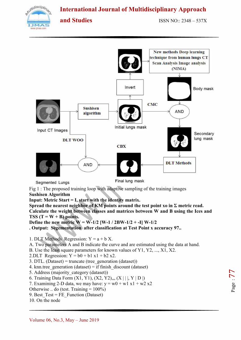
International Journal of Multidisciplinary Approach
and Studies ISSN NO:: 2348 – 537X
Volume 06, No.3, May – June 2019
Pag
e : 7
7
Fig 1 : The proposed training loop with adaptive sampling of the training images
Sushisen Algorithm
Input: Metric Start = I, start with the identity matrix.
Spread the nearest neighbor of KM points around the test point xo in Σ metric read.
Calculate the weight between classes and matrices between W and B using the Ices and
TSS (T = W + B) points.
Define the new metric W = W-1/2 [W-1 / 2BW-1/2 + -I] W-1/2
. Output: Segementation after classification at Test Point x accuracy 97..
1. DLT Methods Regression: Y = a + b X.
A. Two parameters A and B indicate the curve and are estimated using the data at hand.
B. Use the least square parameters for known values of Y1, Y2, ..., X1, X2.
2.DLT Regression: Y = b0 + b1 x1 + b2 x2.
3. DTL. (Dataset) = truncate (tree_generation (dataset))
4. knn.tree_generation (dataset) = if finish_discount (dataset)
5. Address (majority_category (dataset))
6. Training Data Form (X1, Y1), (X2, Y2),,, (X | | |, Y | D |)
7. Examining 2-D data, we may have: y = w0 + w1 x1 + w2 x2
Otherwise .. do (test. Training = 100%)
9. Best_Test = FE_Function (Dataset)
10. On the node
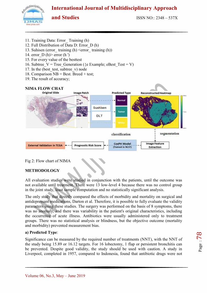
International Journal of Multidisciplinary Approach
and Studies ISSN NO:: 2348 – 537X
Volume 06, No.3, May – June 2019
Pag
e : 7
8
11. Training Data: Error_ Training (h)
12. Full Distribution of Data D: Error_D (h)
13. Suhisen (error_ training (h) <error_ training (h))
14. error_D (h)> error (h ')
15. For every value of the besttest
16. Subtree_V = Tree_Generation ({e Example; eBest_Test = V)
17. In the (best_test, subtree_v) node
18. Comparison NB = Best. Breed + test;
19. The result of accuracy;
NIMA FLOW CHAT
Fig 2: Flow chart of NIMA
METHODOLOGY
All evaluation studies were studied in conjunction with the patients, until the outcome was
not available until treatment. There were 13 low-level 4 because there was no control group
in the joint study, least sample computation and no statistically significant analysis.
The only study that directly compared the effects of morbidity and mortality on surgical and
antidepressant medications, Darton et al. Therefore, it is possible to fully evaluate the validity
parameters using these studies. The surgery was performed on the basis of 8 symptoms, there
was no anomaly, and there was variability in the patient's original characteristics, including
the occurrence of acute illness. Antibiotics were usually administered only to treatment
groups. There was no statistical analysis or blindness, but the objective outcome (mortality
and morbidity) prevented measurement bias.
a) Predicted Type:
Significance can be measured by the required number of treatments (NNT), with the NNT of
the study being 15.89 or 16.12 targets. For 16 lobectomy, 1 flap or persistent bronchitis can
be prevented. Despite good validity, the study should be used with caution. A study in
Liverpool, completed in 1957, compared to Indonesia, found that antibiotic drugs were not

International Journal of Multidisciplinary Approach
and Studies ISSN NO:: 2348 – 537X
Volume 06, No.3, May – June 2019
Pag
e : 7
9
validated with different sociology and ethnicities. The problem found in the study is also
different from the case
Other literature did not evaluate the control group and, therefore, could not assess the
validity. One aspect of computational imports is the test incidence rate (EER), which defines
the ratio of patients with outcomes compared to total subjects. For mortality, ERR ranged
from 0 to 13%, and the incidence of illness was 0 to 38%.
b) Reconstruct Map
Primary tuberculosis after early infection of MDP. In children, mature tuberculosis can lead
to bronchial obstruction and ventricular dysfunction. 15 complications can cause breathing
difficulties, so the decision to undergo surgery or conventional therapy should be addressed.
There was no guidance in decision making, which created controversy about the patient's
eligibility and when to perform 15 surgeries
Validity defines the validity of the study. Cameron et al have not shown the underlying
characteristic of the subjects and the treatment objective of the analysis. There may be
deceptive factors that affect the outcome of the study. [13] Surgery cannot be blinded to
treatment, so there must be an objective reduction in the dependence effect. From the 13
major analyzes of the literature, there are many points to note.
c) Segmentation of feature extraction
1. Includes multiple holes> 1 flap
2. The large cavity consists of> 2 adjacent folds
3. The large cavity contains a significant paranoid ulcer and is unable to partially implant
4. Pores with signs of knot disease
5. Major tracheal branch stenosis
d) Classification of coxPH model
1. Unilateral pits are limited to a specific area where there is no improvement after
conservative treatment
2. Increase the pressure in the cavities
3. Diagnosis, secondary to bronchitis, cavity and endopranchial obstruction
In addition, other signs of surgery include:
1. The case of immunity towards conservative treatment
2. Lung of advanced and irreversible chronic fibroids
Antide pressolysis was performed postoperatively to reduce disease activity and proved to be
a good outcome in surgery. Careful selection was necessary to treat lung tuberculosis
patients. Cameron et al found that 31 patients who were injured in the non-surgical section
had not been reactivated, concluding that surgery was not recommended to prevent
complications.
Mortality was higher among surgical patients, but the baseline characteristics of the groups
were different and patients in poor condition underwent surgery. On the other hand,
comparisons of efficacy of surgery and conventional therapy for children with complex lung
tuberculosis are unethical.

International Journal of Multidisciplinary Approach
and Studies ISSN NO:: 2348 – 537X
Volume 06, No.3, May – June 2019
Pag
e : 8
0
e) Prognotic Risk score
In this case, the patient had many symptoms, such as an unresponsive small child and an
anatomical ulcer that showed chest x-ray and CT scan. It called for surgical evaluation with
six review literature
r
i
ii
r
i
r
i
iiii
xxN
xxxN
k
1
2
1 1
)(
)(ˆ
16082191903973602162261
r
i
iix
16082191903973602162261
r
i
iix
9677.0382,124,12480
382,124,116082480ˆ2
k
IMPLEMENTATION
a)Data Set
This analysis for the three datasets (DLT-WOO,CMC,CMC) used by us Dataset made
available by the National Library Science. 326 with normal cases and 336 with its 662
pictures. Tuberculosis cancer case With each CXR image, a brief report This includes the
patient's age, gender and diagnosis. All X-ray images are not the same size, but 3K X 3K can
be better. Around. Second dataset is Indian Dataset This CMC works for Vellore. There are
56 common cases In the .jpg format, 70 cases of tuberculosis have been given. The resolution
of images varies from 1.5K to 1.5K to 2.7k.
b) Computation phase
(1) We use the algorithm in to calculate X-ray image of the model. This pattern produces a
Maps are probably more similar sets and then defines transforming mapping original
patient's X-ray image registration.
Fig3:(a) data set segmentation Phase CMC image (b) Result CMC dataset NIMA value
Type
Features
DLT WOO
Data
Features
CMC,CBX
Proposed
Features
New
Method
Sushisen 85.5 88.25 96.77
DLT 82.5.5 85.46 88.84

International Journal of Multidisciplinary Approach
and Studies ISSN NO:: 2348 – 537X
Volume 06, No.3, May – June 2019
Pag
e : 8
1
(2) The rib map is doubled further along the range of 0.5 950 (this value) with all the
connected components Dataset needs to be modified based on pixels Removed to get cleaner
rib map It is being done Further calculation in any false margin.
Fig :4 (a) data set segmentation CBX image (b) Result CBX dataset NIMA value
(3) Around the area that detects the costphronic angle Only 20% of the area's two lungs are
considered For further calculation. This percentage should be of the value Tune in based on
your data-set.
Fig 5: (a) data set DLT-WOO segmentation image (b) Result DLT-DOO NIMA
value
(4) For the revised image, we have calculated indexed points the last non-zero points are the
lungs of the costoffrenic angle For each column of the image.
Type
Features
DLT
WOO
Data
Features
CMC,CB
X
Proposed
Features
New
Method
Sushis
en
85.5
88.25
96.33
DLT
82.5.5
85.46
78.84
Type
Features
DLT
WOO
Data
Features
CMC,CBX
Proposed
Features
New Method
Sushisen 81.5 78.25 92.77
DLT 82.5 82.16 78.24

International Journal of Multidisciplinary Approach
and Studies ISSN NO:: 2348 – 537X
Volume 06, No.3, May – June 2019
Pag
e : 8
2
(a) Real dataset result (b) real data set results
(5) Using a binary rib map of gradient computed is a sobel Operator To avoid any fraudulent
calculations At the end of the lung, the interval is not the same), we only remove In the 20%
internal area, calculate high for each lung.
Fig 6: (a) data set all segmentation
image (b) Result all NIMA value
RESULT
Study is an Evidence-Based Case Report. Medline, Proquest, and Cynadirect are synonyms
have been added in a wide range of search results, including "lungs", "operation" and "hair
disease". literature search, six articles were selected and then withdrawn in Table 1. Most of
the studies were done before the era of many antituberbularis regimens. Primary tuberculosis
surgery after standard treatment with leptocycin (Strape) and para-aminosalicylic examined
48 cases of pulmonary TB in children with segmental lesion complications from 2015 to
2019. Based on the results of bronchoscopy after adequate oral therapy, five patients were
rescued. The traditional treatment group was not given antibiotics, but was rested in bed and
was observed intensely in the ward. Reported 101 cases of pulmonary tuberculosis in
children. Primary tuberculosis complications were present in 69,3% of cases. 9 Feltis and
Campbell reported a potential colleague, who had undergone surgery with 47 children with
pulmonary tuberculosis. A study by surgery, persistent cavity, fibonodular disease, atllectasis,
Type
Features
DLT
WOO
Data
Features
CMC,CBX
Proposed
Features
New Method
Sushisen 81.5 78.25 92.77
DLT 82.5 82.16 78.24
Type
Featur
es
DLT
WOO
Data
Features
CMC,CBX
Proposed
Features
New Method
Sushisen 85.5 88.25 96.77
DLT 82.5.5 85.46 88.84

International Journal of Multidisciplinary Approach
and Studies ISSN NO:: 2348 – 537X
Volume 06, No.3, May – June 2019
Pag
e : 8
3
and lost lung / lobe 10 quinlan et al. Cavity, bronchiectasis, waste lung / lobe and middle ear
syndrome.
(a) (b)
Fig: 7 (a) segmentation uncertainty map computed using the proposed method, (b) the same
for Platt scaling method
Fig:8 Over all image the final segmentation obtained methods with sushisen algorithm, Types %
AC %
PC %
FC %C
M CT RS MF TT FR LF MM
CMC 6,365
5,026
4,179
2,517
1,990
1,452
1,352
1,250
599 442 497
CBX 32 122 135 211 303 288 429 764 709 427 702
DLT WOO 69 1,090
2,585
4,254
4,868
4,573
4,686
4,333
4,127
3,622
3,157
Sushisen algorithm
87 478 983 2,865
3,609
4,219
4,884
5,683
8,188
8,334
9,591
DLT 0 0 21 159 454 687 1040 1356 1083 1167 2026
Table 1: New segmentation uncertainty estimation in terms of the accuracy of the final
segmentation after DLT Methods fitting

International Journal of Multidisciplinary Approach
and Studies ISSN NO:: 2348 – 537X
Volume 06, No.3, May – June 2019
Pag
e : 8
4
COMPARISON STUDY
TABLE 2: NIMA Comparison Study
Classifier Three data set
Dataset
Number of
Test
Attributes
Correctly
Classified
Attributes
Classification
rate (%)
Sushisen algorithm
(proposed)
DLT WOO Dataset 1200 1150 97.77
CBX.CMC
Dataset
1200 1160 97.77
KNN ABC Dataset 1200 1020 85
PSO Dataset 1200 980 81.67
NP PSO Data set 1200 990 82,5
ABC Dataset 1200 940 78.33
The performance of the Sushisen algorithms is better than KNN and NP. Table V explains the
Comparison of algorithms - BABC, KNN and NP. Fig. 1 shows the performance analysis of
the algorithms which Table V explains in a bar chat. Fig. 2 exhibits the performance analysis
of the algorithms using Multidimensional to show the algorithm Sushisen is better than KNN
and NP in extracting the details according to the user’s need with better accuracy.
a)System Description
The Toshiba Portege R600 U2530 laptop is powered by Intel Core 2 Duo SU9400, 1400
Mega Hertz (Mhz) processor. This Portege series laptop from Toshiba comes with 3072
Megabytes (MB) of RAM, which is expandable up to Megabytes (MB). Toshiba Portege
R600 U2530 laptop or notebook PC has a 128Solid State Drive Gigabytes (GB) hard disk
capacity, and HDMI Port. The display of Toshiba Portege R600 U2530 is with 1280 x 800
pixels resolution. This Toshiba laptop has a battery life of hours and weighs around 1 kgs.
Operation system Windows 10 running the MATLAB Software programming.
CONCLUSION
In this study, we have proposed a method for detecting tuberculosis From lung radiograph
Our focus is on building aspects for the personal manifestations of tuberculosis using cancer
specified in DLT WOO .Most of the work existing in the field is based on construction
Features to show formatting and layout information Lungs. But many CXR films overlap
body structures are also distorted by acquisitions Noise goes to the wrong information Size
and design details. Such features do not apply. The size is very large and is not well-
normalized for others In the data set We tried to see the indirect effects of lungs on the lungs
Abnormalities rather than directly analyzing the severity Change. The features are based on
what points Radiologists see the X-ray image. We achieved great results Compared to the
refined CMC working in the Indians Dataset But since no direct comparison is possible
Dataset differences Our feature vector is almost the same Tenth part of the length of the
description of the size and design Performance oriented TB detection system is analyzed
Area of receiver working under (AUC) rules (ROC) curve For the removed section, we
follow the following procedure Per column Retrieve index with non-zero values and all
pixels and take it in column of the left and right lungs, respectively. Factors Calculate the

International Journal of Multidisciplinary Approach
and Studies ISSN NO:: 2348 – 537X
Volume 06, No.3, May – June 2019
Pag
e : 8
5
difference between two consecutive factors Each array to get the difference range And it
stores the rib's width and Sushisen algorithm using constant lines in intervals In fact we really
can not only remove the ribs with rows Distance is always different because each rib map is
different Whether or not the rib space is attacked on odd lines We are not aware of the
starting point. To estimate took one Each category of average is indicated 97.77% accuracy.
REFERENCES
i. Anas, E.M.A., Nouranian, S., Mahdavi, S.S., Spadinger, I., Morris, W.J., Salcudean,
S.E., Mousavi, P., Abolmaesumi, P., 2017. Clinical target-volume delineation in
prostate brachytherapy using residual neural networks. In: International Conference
on Medical Image Computing and Computer-Assisted Intervention. Springer, pp.
365–373.
ii. Barra, V., Boire, J.-Y., 2001. Automatic segmentation of subcortical brain structures
in mr images using information fusion. IEEE Trans. Med. Imag. 20 (7), 549–558.
iii. Betrouni, N., Vermandel, M., Pasquier, D., Maouche, S., Rousseau, J., 2005.
Segmentation of abdominal ultrasound images of the prostate using a priori
information and an adapted noise filter. Comput. Med. Imag. Graph. 29 (1), 43–51.
iv. Blake, A., Curwen, R., Zisserman, A., 1993. A framework for spatiotemporal control
in the tracking of visual contours. Int. J. Comput. Vis. 11 (2), 127–145.
v. Choromanska, A., Henaff, M., Mathieu, M., Arous, G.B., LeCun, Y., 2015. The loss
surfaces of multilayer networks. In: Artificial Intelligence and Statistics, pp. 192–204.
vi. Cootes, T.F., Taylor, C.J., Cooper, D.H., Graham, J., 1995. Active shape models-their
training and application. Comput. Vis. Image Understand. 61 (1), 38–59.
vii. Elhamifar, E., Vidal, R., 2013. Sparse subspace clustering: algorithm, theory, and
applications. IEEE Trans. Pattern Anal. Mach. Intell. 35 (11), 2765–2781.
viii. Gal, Y., 2016. Uncertainty in Deep Learning. University of Cambridge. Gal, Y.,
Ghahramani, Z., 2015. Bayesian convolutional neural networks with Bernoulli
approximate variational inference. arXiv: 1506.02158.
ix. Ghavami, N., Hu, Y., Bonmati, E., Rodell, R., Gibson, E., Moore, C., Barratt, D.,
2018. Integration of spatial information in convolutional neural networks for
automatic segmentation of intraoperative transrectal ultrasound images. J. Med. Imag.
6
x. (1), 011003.
xi. Ghose, S., Oliver, A., Martí, R., Lladó, X., Vilanova, J.C., Freixenet, J., Mitra,
J.,Sidibé, D., Meriaudeau, F., 2012. A survey of prostate segmentation methodologies
in ultrasound, magnetic resonance and computed tomography images. Comput.
Method. Progr. Biomed. 108 (1), 262–287.
xii. Ghose, S., Oliver, A., Mitra, J., Martí, R., Lladó, X., Freixenet, J., Sidibé, D.,
Vilanova, J.C., Comet, J., Meriaudeau, F., 2013. A supervised learning framework of
statistical shape and probability priors for automatic prostate segmentation in
ultrasound images. Med. Image Anal. 17 (6), 587–600.

International Journal of Multidisciplinary Approach
and Studies ISSN NO:: 2348 – 537X
Volume 06, No.3, May – June 2019
Pag
e : 8
6
xiii. Gibson, E., Hu, Y., Ghavami, N., Ahmed, H.U., Moore, C., Emberton, M., Huisman,
H.J.,Barratt, D.C., 2018. Inter-site variability in prostate segmentation accuracy using
Deep learning. In: International Conference on Medical Image Computing and
Computer-Assisted Intervention. Springer, pp. 506–514.
xiv. Goodfellow, I., Bengio, Y., Courville, A., Bengio, Y., 2016. Deep Learning, 1. MIT
press
xv. Cambridge. Guo, C., Pleiss, G., Sun, Y., Weinberger, K.Q., 2017. On calibration of
modern neural networks. arXiv: 1706.04599.
xvi. Hodge, A.C., Fenster, A., Downey, D.B., Ladak, H.M., 2006. Prostate boundary
segmentation from ultrasound images using 2d active shape models: optimisation and
extension to 3d. Comput. Method. Progr. Biomed. 84 (2), 99–113.
xvii. Huang, G., Liu, Z., Weinberger, K.Q., van der Maaten, L., 2017. Densely connected
convolutional networks. In: Proceedings of the IEEE Conference on Computer Vision
and Pattern Recognition, 1, p. 3.
xviii. Jemal, A., Bray, F., Center, M.M., Ferlay, J., Ward, E., Forman, D., 2011. Global
cancer statistics. CA: A Cancer J. Clin. 61 (2), 69–90.
xix. Jendoubi, A., Zeng, J., Chouikha, M.F., 2004. Segmentation of prostate ultrasound
images using an improved snakes model. In: Signal Processing, 2004. Proceedings.
ICSP’04. 2004 7th International Conference on, 3. IEEE, pp. 2568–2571.
xx. Ji, P., Zhang, T., Li, H., Salzmann, M., Reid, I., 2017. Deep subspace clustering
networks. In: Advances in Neural Information Processing Systems, pp. 23–32.
xxi. Kachouie, N.N., Fieguth, P., Rahnamayan, S., 2006. An elliptical level set method for
automatic TRUS prostate image segmentation. In: Signal Processing and Information
Technology, 2006 IEEE International Symposium on. IEEE, pp. 191–196.
xxii. Karimi, D., Zeng, Q., Mathur, P., Avinash, A., Mahdavi, S., Spadinger, I.,
Abolmaesumi, P., Salcudean, S., 2018. Accurate and robust segmentation of the
clinical target volume for prostate brachytherapy. In: Frangi, A.F., Schnabel, J.A.,
Davatzikos, C., Alberola-López, C., Fichtinger, G. (Eds.), Medical Image Computing
and Computer Assisted Intervention – MICCAI 2018. Springer International
Publishing, Cham, pp. 531–539.
xxiii. Kendall, A., Cipolla, R., 2016. Modelling uncertainty in deep learning for camera
relocalization. In: 2016 IEEE International Conference on Robotics and Automation
(ICRA). IEEE, pp. 4762–4769.
xxiv. Kendall, A., Gal, Y., 2017. What uncertainties do we need in Bayesian deep learning
for computer vision? In: Advances in Neural Information Processing Systems, pp.
5574–5584.
xxv. Kingma, D.P., Ba, J., 2014. Adam: a method for stochastic optimization. In:
Proceedings of the 3rd International Conference on Learning Representations (ICLR).
Kohavi, R., Wolpert, D.H., et al., 1996. Bias plus variance decomposition for zero-
one loss functions. ICML, 96. 275–83
International Journal of Multidisciplinary Approach
and Studies ISSN NO:: 2348 – 537X
Volume 06, No.3, May – June 2019
Pag
e : 8
7
xxvi. Kuncheva, L., Whitaker, C., 2003. Measures of diversity in classifier ensembles and
their relationship with the ensemble accuracy. Mach. Learn. 51 (2), 181–207.
xxvii. Lakshminarayanan, B., Pritzel, A., Blundell, C., 2017. Simple and scalable predictive
uncertainty estimation using deep ensembles. In: Advances in Neural Information
Processing Systems, pp. 6402–6413.
xxviii. Li, X., Li, C., Fedorov, A., Kapur, T., Yang, X., 2016. Segmentation of prostate from
ultrasound images using level sets on active band and intensity variation across edges.
Med. Phys. 43 (6Part1), 3090–3103.
xxix. Mahdavi, S.S., Chng, N., Spadinger, I., Morris, W.J., Salcudean, S.E., 2011. Semi-
automatic segmentation for prostate interventions. Med. Image Anal. 15 (2),226–237.
xxx. Milletari, F., Navab, N., Ahmadi, S.-A., 2016. V-net: fully convolutional neural
networks for volumetric medical image segmentation. In: 3D Vision (3DV), 2016
Fourth International Conference on. IEEE, pp. 565–571.
xxxi. Morris, W.J., Keyes, M., Spadinger, I., Kwan, W., Liu, M., McKenzie, M., Pai, H.,
Pickles, T., Tyldesley, S., 2013. Population-based 10-year oncologic outcomes after
low-dose-rate brachytherapy for low-risk and intermediate-risk prostate cancer.
Cancer 119 (8), 1537–1546.
xxxii. Mozaffari, M.H., Lee, W., 2016. 3d ultrasound image segmentation: a survey. arXiv:
xxxiii. 1611.09811.
xxxiv. Naeini, M.P., Cooper, G.F., Hauskrecht, M., 2015. Obtaining well calibrated
probabilities using Bayesian binning. In: AAAI, pp. 2901–2907.
xxxv. Nag, S., Bice, W., DeWyngaert, K., Prestidge, B., Stock, R., Yu, Y., 2000. The
American brachytherapy society recommendations for permanent prostate
brachytherapy postimplant dosimetric analysis. Int. J. Radiat. Oncol. Biol. Phys. 46
(1), 221–230.
xxxvi. Neal, R.M., 2012. Bayesian Learning for Neural Networks, 118. Springer Science &
Business Media. Noble, J.A., Boukerroui, D., 2006. Ultrasound image segmentation:
a survey. IEEE Trans. Med. Imag. 25 (8), 987–1010.
xxxvii. Nouranian, S., Mahdavi, S.S., Spadinger, I., Morris, W.J., Salcudean, S.E.,
Abolmaesumi, P., 2015. A multi-atlas-based segmentation framework for prostate
brachytherapy. IEEE Trans. Med. Imag. 34 (4), 950–961.
xxxviii. Nouranian, S., Ramezani, M., Spadinger, I., Morris, W.J., Salcudean, S.E.,
Abolmaesumi, P., 2016. Learning-based multi-label segmentation of transrectal
ultrasound images for prostate brachytherapy. IEEE Trans. Med. Imag. 35 (3), 921–
932.
xxxix. Pawlowski, N., Brock, A., Lee, M.C., Rajchl, M., Glocker, B., 2017. Implicit weight
uncertainty in neural networks. arXiv: 1711.01297.
View publication statsView publication stats
See discussions, stats, and author profiles for this publication at: https://www.researchgate.net/publication/337532404
Image fusion on PET/ MRI Images Using Inverse Wavelet decomposition
Transform
Article · June 2019
CITATIONS
0READS
36
2 authors, including:
Some of the authors of this publication are also working on these related projects:
Pulmonary nodule identification View project
Deep Learning Algorithms View project
Piramu Kailasam
Sadakathullah Appa College
16 PUBLICATIONS 10 CITATIONS
SEE PROFILE
All content following this page was uploaded by Piramu Kailasam on 26 November 2019.
The user has requested enhancement of the downloaded file.

© 2019 IJRAR June 2019, Volume 6, Issue 2 www.ijrar.org (E-ISSN 2348-1269, P- ISSN 2349-5138)
IJRAR19K4195 International Journal of Research and Analytical Reviews (IJRAR)www.ijrar.org 436
Image fusion on PET/ MRI Images Using Inverse
Wavelet decomposition Transform
ABSTRACT In this paper a simple and improved medical fusion approaches for PET / MRI images. Image fusion produces merging of two or more images to get the most relevant characteristics of image. The input image is applied by discrete wavelet transform technique to get synthesized image. This paper focuses on applying wavelet decomposition method inverse discrete wavelet decomposition method on PET / MRI images in pixel and structure level. The resultant fused image preserves the possible important information from input images and not introduce artefacts also noises reduces in maximum extent. The parameters MSE, PSNR, RMSE showed good results for PET / MRI images. Keywords : Image Decomposition, Positron Emission Tomography, iDWT, Fused image INTRODUCTION Positron emission tomography has been utilized in various medical diognosis applications[1-3]. PET or SPECT data require an activity map of radiotracer distribution of the lung or brain scan images. PET images are suffered by notable noises, because of dosage and image acquisition in seconds. Hounsfield greater than 600 were considered to be bone after thresholding process in CT images. The attenuation maps were helpful to identify bone tissue. A high noise in PET images lead to diagnosis the type of diseases. PET scans generate 3D images of ROI. A shrived substance tracer in injected and traced throughout the blood circulation to attain target are of interest. If a positron interacts with anklectron , which generates 2 gamma photons in opposite directions . The PET detector array scanner measured the photons. So it impossible to locate the current active region and organ activity also revealed. A radio nuclide is (18F) flurodexyglucose (FDG) which is short lived nature in PET scanner. Due to low resolution of PET image it is combined CT or MRI data to enhance the functional data. This requires the registration of the generated volumetric PET /CT/MRI datasets. The registration of image in however difficult since the scanned object has to moved to another prescribed scanner. This causes the position and orientation of the object. This complicates the matching of ROIs. These are aggravated by multilevel of resolution of image. This CT/MRI/PET/SPECT data renders the matching of properties difficult. Thus the PET scanning is costlier than other modalities. PET scanner have good ability to characterize the metabolite activity. Added with it is good in searching for metastases of cancer. The reconstruction of the PET image diagnosed region area , the expectation maximization is adopted. This gives a maximum likelihood estimate. The ML-DM accurately find the position noise characters from many iterations of PET data. This increases the noises of PET hence the quality of the images decreases. In order to reduce noise we need preknowledge of image data for reconstruction process. Post filtering has been applied in some PET devices. Gaussian filtering used for Post filtering process. Gaussian filter is a linear low pass filter also a filter mask has in bell shaped curve with centre and symmetric tapering section in either side . The weights of Gaussian filter are calculated using Gaussian function. The NLM an d BM3D algorithm constantly suggested for denoising process in recent upcoming times. In the clinical diagnosis, the problems regarding images like MRI-PET, CT-PET, and CT-MRI were discussed frequently in medical field. So as to provide more useful information for clinical diagnosis, there is a necessity to combine useful information from various device images. SPECT – CT are useful to study about vascular blood flow test in abdominal and ultrasound images [1]. The integrated scanners perform in immediate sequence without changing the patients position. The improved images will enable doctors to see the condition of organs of astronauts hearts, which is a NASA project in space[2]. Image Fusion can be categorized in to pixel level , feature level , signal level and decision level. Pixel level image fusion is going to discussion in upcoming sections. Image fusion based on wavelet multiresolution technique followed by PCA technique in given in next section. Comparative analysis is brought by section also continued by Conclusion section. II.Material and Methods Pixel or Spatial Level Image Fusion Image fusion can be done by many methods like technical fusion, multiplicative fusion, subtractive fusion, PCA fusion, IHS fusion , Brovery , Color related technique and wavelet technique. The source image combined with single
Dr. M. Mohamed Sathik,Principal,Sadakathullah Appa College,Tirunelveli,India S Piramu Kailasam,Assistant Professor,Sadakathullah Appa College,Tirunelveli,India
USER
Underline
USER
Underline
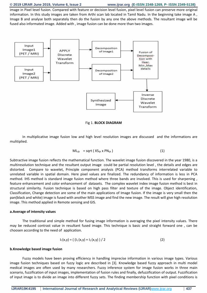
© 2019 IJRAR June 2019, Volume 6, Issue 2 www.ijrar.org (E-ISSN 2348-1269, P- ISSN 2349-5138)
IJRAR19K4195 International Journal of Research and Analytical Reviews (IJRAR)www.ijrar.org 437
image in Pixel level fusion. Compared with feature or decision level fusion, pixel level fusion can preserve more original information. In this study images are taken from Arthi scan lab located in Tamil Nadu. In the beginning take image A , Image B and analyse both separately then do the fusion by any one the above methods. The resultant image will be fused also informated image. Added with , image fusion can be done more than two images.
Fig 1. BLOCK DIAGRAM In multiplicative image fusion low and high level resolution images are discussed and the informations are mulitiplied. MLijk = sqrt ( XSijk x PNijk ) (1) Subtractive image fusion reflects the mathematical function. The wavelet image fusion discovered in the year 1980, is a multiresolution technique and the resultant output image could be partial resolution level , the details and edges are distorted. Compare to wavelet, Principle component analysis (PCA) method transforms interrelated variable to unrelated variable in spatial domain. Here pixel values are finalized. The redundancy of information is less in PCA method. IHS method is standard image fusion method where three bands are involved. This is used for sharpening , feature enhancement and color enhancement of datasets. The complex wavelet index image fusion method is best in structural similarity. Fusion technique is based on high pass filter and texture of the image. Object identification, Classification, Change detection are some of the main applications of Image fusion. If the image is very small then the pan(black and white) image is fused with another MSS image and find the new image. The result will give high resolution image. This method applied in Remote sensing and GIS. a.Average of intensity values The traditional and simple method for fusing image information is averaging the pixel intensity values. There may be reduced contrast value in resultant fused image. This technique is basic and straight forward one , can be choosen according to the need of application. If (x,y) = ( (I1 (x,y) + I2 (x,y) ) / 2 (2) b.Knowledge based image fusion Fuzzy models have been proving efficiency in handling imprecise information in various image types. Various image fusion techniques based on fuzzy logic are described in [3]. Knowledge based fuzzy approach in multi model medical images are often used by many researchers. Fuzzy inference system for image fusion works in three main scenario, fuzzification of input images, implementation of fusion rules and finally, defuzzification of output. Fuzzification of input image is to divide an image into different fuzzy sets. The finding membership function with pixel conditions is
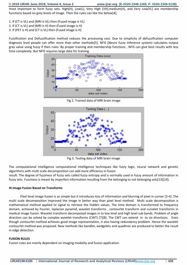
© 2019 IJRAR June 2019, Volume 6, Issue 2 www.ijrar.org (E-ISSN 2348-1269, P- ISSN 2349-5138)
IJRAR19K4195 International Journal of Research and Analytical Reviews (IJRAR)www.ijrar.org 438
most important to form fuzzy sets. High(H), Low(L), Very High (VH),medium(H), and Very Low(VL) are membership functions based on grey levels of image. Then the rules can like the below[4], 1. If (CT is VL) and (MRI is VL) then (Fused image is VL) 2. If (CT is VL) and (MRI is H) then (Fused image is H) 3. If (PET is H) and (CT is VL) then (Fused image is H) Fuzzification and Defuzzification method reduces the processing cost. Due to simplicity of defuzzification computer diagnosis level people can offer more than other methods[5]. NFIS (Neuro fuzzy Inference system) calculates output gray value using fuzzy if then rules. By proper training and membership functions , NFIS can give best results with less time complexity. But NFIS requires large data for training.
Fig 2. Trained data of MRI brain image
Fig 3. Testing data of MRI brain image
The computational intelligence computational intelligence techniques like fuzzy logic, neural network and genetic algorithms with multi scale decomposition can add more efficiency in fusion result. The degree of fuzziness of fuzzy sets called fuzzy entropy and is normally used in fuzzy amount of information in fuzzy sets. Fuzziness is meant by imperfect information resulting from the belonging to not belonging sets[13][14]. III.Image Fusion Based on Transforms Pixel level image fusion is so simple but it introduces loss of information and blurring of pixel in corner [3-4]. The multi scale decomposition improved the image in better way than pixel level method. Multi scale decomposition is mathematical method applied to signal to retrieve the hidden values. The time domain is transformed to frequency domain, achieved by Fourier, laplacian pyramid, wavelet transforms , contourlet transform and curvelet transforms in medical image fusion. Wavelet transform decomposed images in to low level and high level sub bands. Problem of angle direction can be solved by complex wavelet transforms (CWT) [7][8]. The CWT can extend in to six directions. Even though contourlet method achieves good image representation, it also having redundancy problem. Hence the wavelet contourlet method was proposed. New methods like bandlet, wedgelets and quadtree are produced to better the result in edge detection. FUSION RULES Fusion rules are mainly dependent on imaging modality and fusion application.

© 2019 IJRAR June 2019, Volume 6, Issue 2 www.ijrar.org (E-ISSN 2348-1269, P- ISSN 2349-5138)
IJRAR19K4195 International Journal of Research and Analytical Reviews (IJRAR)www.ijrar.org 439
a)Activity level measurement: The amount of information at each pixel measured by energy at each pixel or energy of neighbouring pixels. This is window level measurement . The integer values for n are odd level. The edge level smoothness is good. The size of window may be n x n.
E(i,j) = mod(x(i,j)) or E(i,j) = mod(x(i,j))2 (3) x(i,j) is the gray value of the pixel of image at (i,j) the position. The another window based spatial frequency (SF) given by[9]:
SF = sqrt(RF2 + CF2) (4) where RF and CF are row frequency and column frequnency respectively and calculated by,
RF =√1
𝑀(𝑁−1)𝑁∑ ∑ (𝑥(𝑚, 𝑛 + 1) − 𝑥(𝑚, 𝑛)2) 𝑁−2
𝑛=0𝑀−1𝑚=0 and (5)
CF=√1
𝑀(𝑁−1)𝑁∑ ∑ (𝑥(𝑚 + 1, 𝑛) − 𝑥(𝑚, 𝑛)2)𝑁−1
𝑛=0𝑀−2𝑚=0 (6)
High value of activity level indicates more amount of information in input image. b)Principal Component analysis Principle component analysis is a mathematical tool. The fusion is done by computing weighted averge of images to be fused. If p1 and p2 are normalized component of eigen vector then the fusion rule can be writtern as [15] [16],
If = p1 * I1 + p2 * I2 (7) The input images to be fused I1(x,y), I2(x,y) are arranged in two column vectors and their empirical means are subtracted.
Multiscale Decompostion Wavelet Based Image Fusion In the first step the contrast of image is enhanced using histogram equilzation method. The enhaced images are fused using pixel or transform methods. To enhance the contrast , scaling factor is adopted. Inverse discrete wavelet transform based image fusion The Left image XL and right image XR of the input image is taken. The images applied with DWT with Haar features. The decomposed Left and Right images are then again decomposed with max and mean detail with IDWT transform. The generated synthesized image provides the essential character of input image. PERFORMANCE EVALUATION METRICS a)Fusion Index (FI) It is the combination of IAF and IBF factors. Where IAF is the mutual information index between multispectral image and fused image, IBF is mutual information index between panchromatic image and fused image. This measures affects the quality of an image. The quality of image depends on degree of fusion index. FI = IAF + IBF (8) b)Entropy Entropy is the amount of information present in the image Here P is the probability of pixel xi,
E = -∑ 𝑝(𝑥𝑖) log2𝑝(𝑥𝑖)𝑁𝑖=1 (9)

© 2019 IJRAR June 2019, Volume 6, Issue 2 www.ijrar.org (E-ISSN 2348-1269, P- ISSN 2349-5138)
IJRAR19K4195 International Journal of Research and Analytical Reviews (IJRAR)www.ijrar.org 440
c)Fusion Symmetry (FS) Fusion symmetry is an indicator of the degree of symmetry in the information content from both images.
FS = abs(𝐼𝐴𝐹
(𝐼𝐴𝐹+ 𝐼𝐵𝐹 ) - 0.5) (10)
The lower value of FS indicates better symmetry in the fused image. d)Peak Signal to Noise Ratio (PSNR) The peak signal to noise ratio (PSNR) is the ratio between the maximum value of an image and magnitude of background noises.
PSNR = 10log10 (2𝑛−1)2
𝑀𝑆𝐸 (11)
e)Means squre Error(MSE) It is one the famous used measures to calculate the deviation between the original and fused image data.
MSE =∑ ∑ [𝑅(𝑖,𝑗)−𝐹(𝑖,𝑗)]2𝑁
𝑗=1𝑀𝑖=1
𝑀𝑁 (12)
where i,j are spatial position of pixels and M , N are dimensions of the image.
f)Root Mean Square Error (RMSE) This measurement is used to evaluate the fused image. Let be the fused image, is the input image, then
RMSE = √∑ ∑[𝑅(𝑖,𝑗)−𝐹(𝑖,𝑗)]2
𝑀𝑁 (13)
Result and Discussion The two dimensional wavelet technique is famous in image fusion area. It merges two images . This is the simple and fast compare to previous methods for medical image. The wavelet decomposing of two original images using fusion methods applied to approximation coeggicients and detailed coefficients. Wavelet transform divide the original image into low and high frequency levels. Low level contains the outline information and high level reflects the luminance changes and edge information of an image. The fusion image should contain both information of ROIs. The two images should be in same size and resolution. Peak Signal to Noise Ratio (PSNR) This is a good quality measure in image fusion. It indicates the similarity between the two medical images. The higher the PSNR value gives better fused image. Means squre Error(MSE) It is computed by finding the squared error dived by total number of pixels . The smaller the value , the better fused image. It is difficult to find blur and blocking of aritifacts.
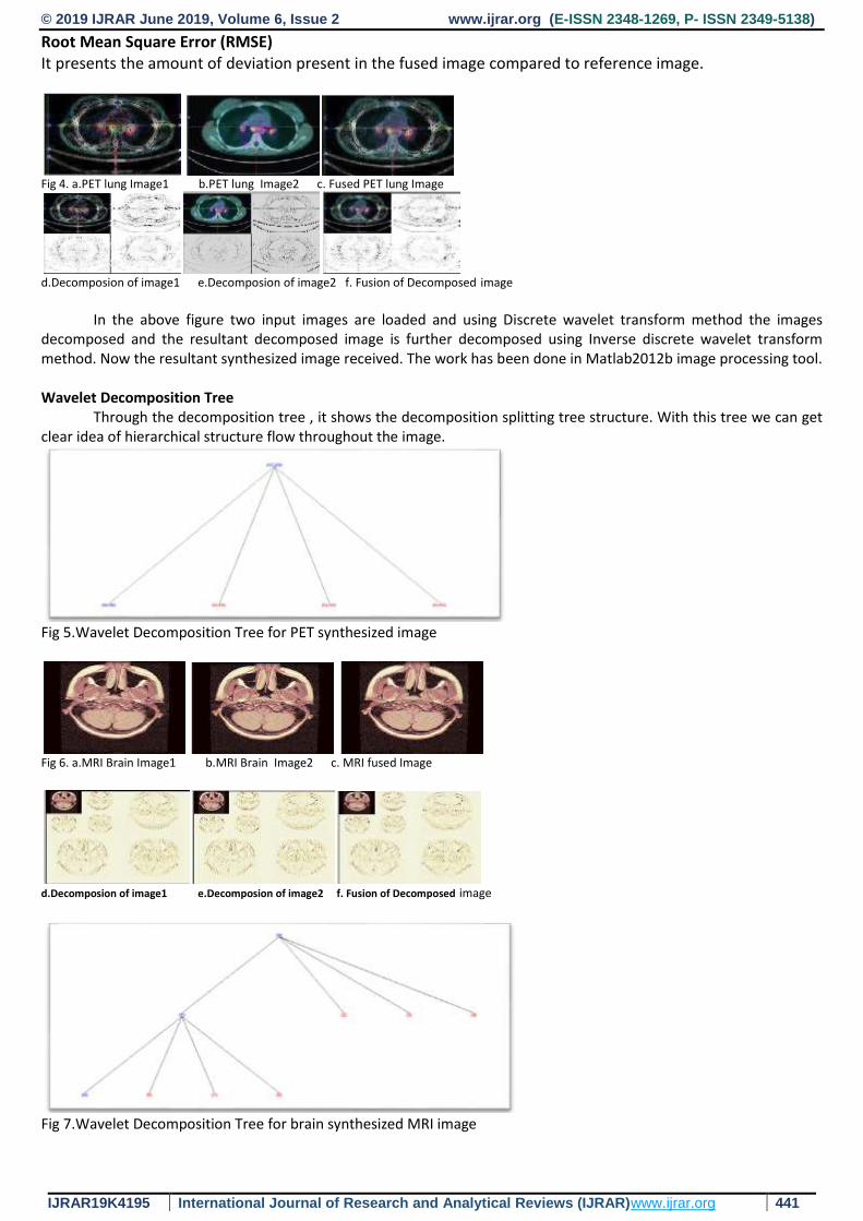
© 2019 IJRAR June 2019, Volume 6, Issue 2 www.ijrar.org (E-ISSN 2348-1269, P- ISSN 2349-5138)
IJRAR19K4195 International Journal of Research and Analytical Reviews (IJRAR)www.ijrar.org 441
Root Mean Square Error (RMSE) It presents the amount of deviation present in the fused image compared to reference image.
Fig 4. a.PET lung Image1 b.PET lung Image2 c. Fused PET lung Image
d.Decomposion of image1 e.Decomposion of image2 f. Fusion of Decomposed image In the above figure two input images are loaded and using Discrete wavelet transform method the images decomposed and the resultant decomposed image is further decomposed using Inverse discrete wavelet transform method. Now the resultant synthesized image received. The work has been done in Matlab2012b image processing tool. Wavelet Decomposition Tree Through the decomposition tree , it shows the decomposition splitting tree structure. With this tree we can get clear idea of hierarchical structure flow throughout the image.
Fig 5.Wavelet Decomposition Tree for PET synthesized image
Fig 6. a.MRI Brain Image1 b.MRI Brain Image2 c. MRI fused Image
d.Decomposion of image1 e.Decomposion of image2 f. Fusion of Decomposed image
Fig 7.Wavelet Decomposition Tree for brain synthesized MRI image

© 2019 IJRAR June 2019, Volume 6, Issue 2 www.ijrar.org (E-ISSN 2348-1269, P- ISSN 2349-5138)
IJRAR19K4195 International Journal of Research and Analytical Reviews (IJRAR)www.ijrar.org 442
Inverse discrete wavelet transform (IDWT) of input or reconstruct signals from subbands with smaller bandwidths and slower sample rates.The IDWT block is the same as the Dyadic Synthesis Filter Bank block in the MultiMate Filters library, but with different default settings.
Fig 8. a.MRI Brain Image1 b.MRI Brain Image2 c. MRI fused Image
d.Decomposion of image1 e.Decomposion of image2 f. Fusion of Decomposed image
Fig 9.Wavelet Decomposition Tree for brain fused image
Fig 10. Fourier Curve fitting for MRI brain images
Fig 11. Gaussian Curve fitting graph for MRI brain images The Gaussian Equation is given as below f(x) = a1*exp(-(x-b1)/c1)^2 (14)
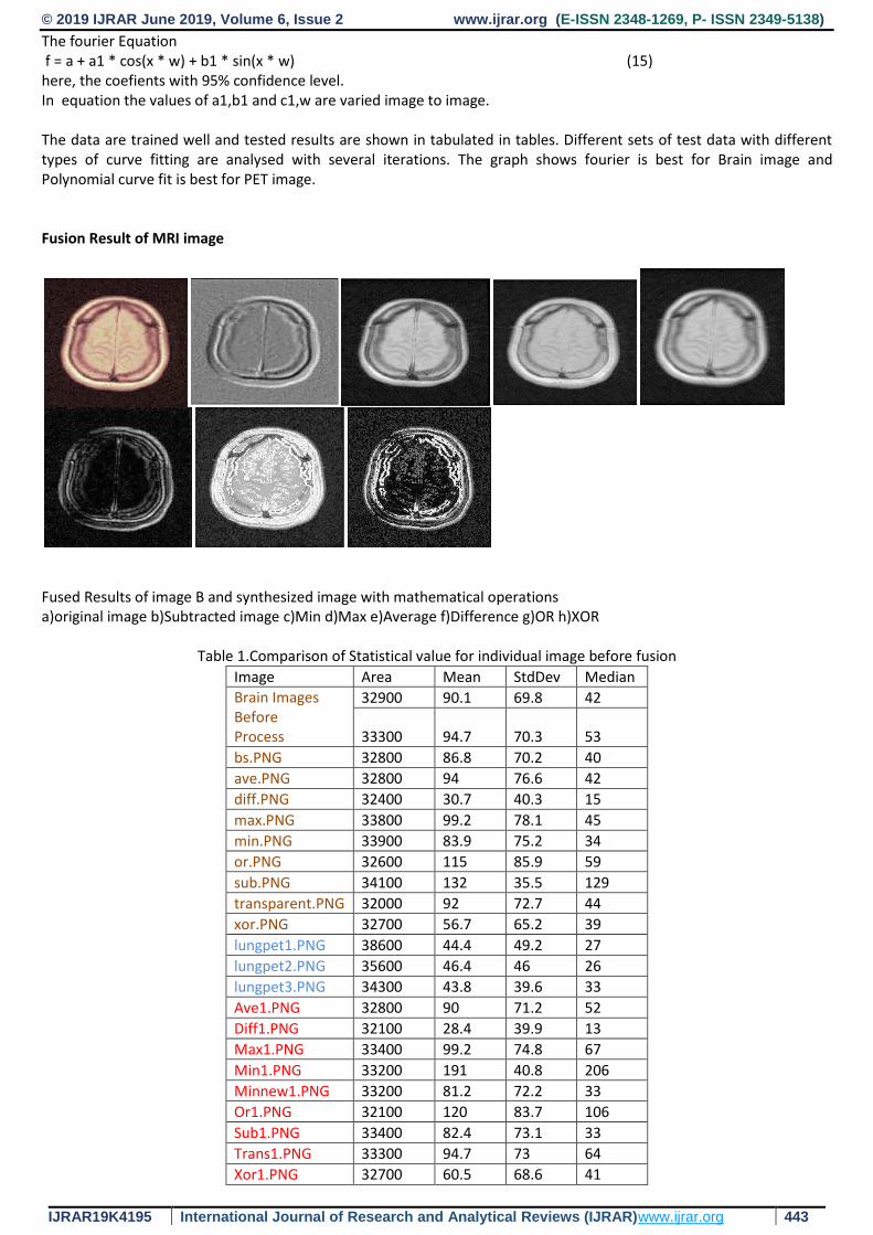
© 2019 IJRAR June 2019, Volume 6, Issue 2 www.ijrar.org (E-ISSN 2348-1269, P- ISSN 2349-5138)
IJRAR19K4195 International Journal of Research and Analytical Reviews (IJRAR)www.ijrar.org 443
The fourier Equation f = a + a1 * cos(x * w) + b1 * sin(x * w) (15) here, the coefients with 95% confidence level. In equation the values of a1,b1 and c1,w are varied image to image. The data are trained well and tested results are shown in tabulated in tables. Different sets of test data with different types of curve fitting are analysed with several iterations. The graph shows fourier is best for Brain image and Polynomial curve fit is best for PET image. Fusion Result of MRI image
Fused Results of image B and synthesized image with mathematical operations a)original image b)Subtracted image c)Min d)Max e)Average f)Difference g)OR h)XOR
Table 1.Comparison of Statistical value for individual image before fusion
Image Area Mean StdDev Median
Brain Images Before Process
32900 90.1 69.8 42
33300 94.7 70.3 53
bs.PNG 32800 86.8 70.2 40
ave.PNG 32800 94 76.6 42
diff.PNG 32400 30.7 40.3 15
max.PNG 33800 99.2 78.1 45
min.PNG 33900 83.9 75.2 34
or.PNG 32600 115 85.9 59
sub.PNG 34100 132 35.5 129
transparent.PNG 32000 92 72.7 44
xor.PNG 32700 56.7 65.2 39
lungpet1.PNG 38600 44.4 49.2 27
lungpet2.PNG 35600 46.4 46 26
lungpet3.PNG 34300 43.8 39.6 33
Ave1.PNG 32800 90 71.2 52
Diff1.PNG 32100 28.4 39.9 13
Max1.PNG 33400 99.2 74.8 67
Min1.PNG 33200 191 40.8 206
Minnew1.PNG 33200 81.2 72.2 33
Or1.PNG 32100 120 83.7 106
Sub1.PNG 33400 82.4 73.1 33
Trans1.PNG 33300 94.7 73 64
Xor1.PNG 32700 60.5 68.6 41

© 2019 IJRAR June 2019, Volume 6, Issue 2 www.ijrar.org (E-ISSN 2348-1269, P- ISSN 2349-5138)
IJRAR19K4195 International Journal of Research and Analytical Reviews (IJRAR)www.ijrar.org 444
Table 1 showed Area, Mean, Standard deviation and Median of the given image. The value calculated according to the equation. The mean value is increased higher in ORed and Subtracted images. It is very low in Difference operation. But , in standard deviation category notably high in ORed image and low in Subtracted image. Table 2.Comparison result of MRI Brain image and synthesized image
Images 1&7 1&2 2&3 2&4 2&5 2&6 2&7 2&8 2&9 2&10
MSE .21 .16 .18 .21 .24 .23 .20 .22 .21 .20
PSNR 54.87 56.22 55.54 54.97 54.30 54.51 55.04 54.76 55.01 55.24
The higher the PSNR (Peak Signal to Noise Ratio) value will be good for image fusion . So according to the table all images having 50% above similarity like input image. In particular image 1 and 2 having psnr value as 56.22. In addition, if you note the MSE value compare to other values image 1 and 2 having .16 value which is reasonable. This table shows that image 1 and image 2 gives less error in both MSE and PSNR parameters.
Table 3. Comparison result of Brain MRI and CT image with T1 contrast with T2 contrast
Image Name
Curve fit type
SSE (x10-2)
R-square Coef RMSE (x10-7)
Brain image1
Gaussian 2.75 .88 3 20.52
Brain image1
Fourier 2.23 .90 4 18.44
PET Image1 Polynomial 1.40 1 2 4.37
PET image1 Gaussian 6.22 .97 3 8.94
Brain image2
Gaussian 2.9 .99 3 5.41
Brain image2
Fourier 6.2 1 4 2.52
Brain image3
Fourier 6.5 1 4 11.61
Brain image3
Fourier 7.0 1 4 2.66
Brain image3
Gaussian 3.26 .99 3 5.75
Prediction errors could be found by root mean square error. Residuals are a measure of how far from the line of data points . Also it tells about data on line of best fit. Root mean square error is commonly used in climatology, forecasting to verify experimental results. In above table the all RMSE values are in x10-7. It shows the the data is having very minor errors. Hence the DWT + iDWT fusion method is successful method. SSE is sum of squared error also very low value. CONCLUSION In this study, pixel level and multiresolution level fusion applied in to CT and MRI images. Each fusion technique is discussed with its merits and demerits. Wavelet image fusion method has been applied successfully to newly formed database with various feature techniques and results are shown and discussed with different parameters. Data base has got from arthi scan centre, tirunelveli. It is impossible to design universal image fusion technique for all type of images for medial applications. In future this could be extend with PCA and CWT technique also can improve the performance of fusion method.
© 2019 IJRAR June 2019, Volume 6, Issue 2 www.ijrar.org (E-ISSN 2348-1269, P- ISSN 2349-5138)
IJRAR19K4195 International Journal of Research and Analytical Reviews (IJRAR)www.ijrar.org 445
REFFERENCES
1. Nemir Al-Azzawi and Wan Ahmed K. Wan Abdullah, Medical Image Fusion Schemes using Contourlet Transform and PCA Based, Annual International Conference of the IEEE, Engineering in Medicine and Biology Society,2009, pp.5813-5816.
2. http://www.nasa.gov/centers/ames/research/2007/imagefusion.html 3. Irshad, H.; Kamran, M.; Siddiqui, A.B.; Hussain, A., Image fusion using computational intelligence:A survey,
Environmental and Computer Science, ICECS ’09. Second International Conference ,2009, pp.128- 132. 4. Jionghua Teng; Suhuan Wang; Jingzhou Zhang; Xue Wang, Fusion algorithm of medical images based on fuzzy
logic, Fuzzy Systems and Knowledge Discovery (FSKD), 2010 Seventh International Conference, vol.2, pp.546-550.
5. Jionghua Teng; Suhuan Wang; Jingzhou Zhang; Xue Wang, Neuro fuzzy logic based fusion algorithm of medical images, Image and Signal Processing (CISP), 2010, 3rd International Congress, vol.4, pp.1552- 1556.
6. R. C. Gonzalea and R. E. Woods, Wavelets and Multiresolution Processing, Digital Image Processing, 2004, 2nd Ed., Prentice Hal.
7. Ivan W. Selesnick, Richard G. Baraniuk, and Nick G. Kingsbury, The Dual-Tree Complex Wavelet Transform, IEEE Signal Processing Magazine, 2005, vol. 22, no. 6, pp. 123-151.
8. Jingyu Yang, Yao Wang, Wenli Xu, and Qionghai Dai, Image Coding Using Dual-Tree Discrete Wavelet Transform, IEEE Trans. Image Processing, 2008, vol. 17, no. 9, pp. 1555-1569.
9. Wang Xue-jun; Mu Ying, A Medical Image Fusion Algorithm Based on Lifting Wavelet Transform, Artificial Intelligence and Computational Intelligence (AICI), 2010 International Conference, vol.3, pp.474-476.
10. Gonzalo Pajares, Jes us Manuel de la Cruz, A wavelet-based image fusion tutorial, Pattern Recognition, 2004, pp.1855 1872.
11. Yong Chai; You He; Chaolong Ying, CT and MRI Image Fusion Based on Contourlet Using a Novel Rule, Bioinformatics and Biomedical Engineering, 2nd International Conference, 2008, vol., no., pp.2064- 2067.
12. L.A.Zadeh, Probability measure of fuzzy events,J.Mathematical analysis and applications,1968, pp.421-427. 13. Zhuanzheng Zhao, YunXiangLi, A Novel Image Fusion Method Based on Fuzzy Contourlet Transform,Computer
and Communication Tech- nologies in Agriculture Engineering (CCTAE), 2010 International Conference, vol.1, pp.404-407.
14. Zhuanzheng Zhao; Yunxiang Li, A novel image fusion method based on fuzzy contourlet transform, Computer and Communication Technologies in Agriculture Engineering (CCTAE), 2010 International Conference,1, no., pp.404,407.
15. Changtao Hea, Quanxi Liub, Hongliang Lia, Haixu Wangb, Multimodal medical image fusion based on IHS and PCA,Procedia Engineering, 2010, pp. 280285.
16. V.P.S. Naidu and J.R. Raol, Pixel-level Image Fusion using Wavelets and Principal Component Analysis, Defence Science Journa, 2008, Vol. 58, No. 3, pp. 338-352.
17. Shen, R.; Cheng, I.; Basu, A., Cross scale coefficient selection for volumetric medical image fusion, IEEE Transactions on Biomedical Engineering, 2012, Volume: PP , Issue: 99.
18. Zhou Wang, Alan C. Bovik., A Universal Image Quality Index, IEEE Signal Processing Letters, 2002, Vol. 9, No. 3. 19. Manjusha Deshmukh, Udhav Bhosale, Image Fusion and Image Quality
20. J.Jenith chritinal,T.Jeemina Jebaselvi,A novel color image fusion for multi sensor night vision images,IJCATR,2013,Vol.2,Issue 2
View publication statsView publication stats

Pulmonary CT Image analysis for Nodule
Detection using Inspired FCM Clustering
Dr. M. Mohamed Sathik
Principal,
Sadakathullah Appa College,
Tirunelveli,India
S Piramu Kailasam,
Assistant Professor ,
PG & Research Department of Computer Science ,
Sadakathullah Appa College, Tirunelveli,
India
Abstract—The segmentation of white blob nodule area from
pulmonary CT images are tedious and time consuming task.
The accuracy of nodules as tumor depends on the radiologist
experience only. Hence the CAD still necessary to overcome
these limitations. In this study to improve the performance
and reduce the complexity of segmentation, adaptive
histogram equalization method and Fuzzy C means applied
with high level iterations. Further to improve the accuracy
local and global threshold also used. The resultant parameters
mean , median showed good accuracy results.
Keyword— Pre-processing; Global Threshold; Fuzzy C
Means(FCM); Segmentation
I. INTRODUCTION
Image Segmentation is the process that segment
an image into many disjoint small area based on the certain
principle, and it is the one of the most basic area of
research in the image processing. Image segmentation is
used in many applications; with Image Retrieval it is
possible to analyse the images in Geology Information
Systems, Medical Image Analysis, Film and Photo
Analysis etc.
II. RELATED WORKS
Many image processing techniques for the
detection of lung cancer by using CT images are reviewed
in [1], lung cancer detection is carried out by splitting the
review in different aspects such as pre-processing, nodule
segmentation and segmentation, lung nodule detection are
presented in [2], the performance of the recent lung nodule
detection techniques are compared. A lung cancer
classification system[3] is proposed on the basis of wavelet
recurrent neural network also employs wavelet to remove the
noise from the input image and the recurrent neural
network is utilized for classification. Perhaps, this author
could not achieve better specificity rates and this implies
that the false positive rates of the work are reasonably
greater. In paper [4], FCM is applied to achieve
segmentation and the GLCM (Gray Level Co - occurence
Matrix) features are extracted. The author Manasee[5]
says a lung cancer detection technique that relies on genetic
approach is proposed, this work involves more time
complexity and the number of connected objects have been
calculated by assigning 1 to inside and 0 to outside of the
object that shows the medical image based on threshold
technique to analyze the performance.
A. Segmentation Techniques
Some of the image segmentation methods are
Local entropy image segmentation [6]. A Discrete cosine
texture feature is applied by [7].The parallel algorithm for
grey scale image was clearly declared[8]. Clustering of
spatial patterns and watershed algorithm[9] is done.
Medical image segmentation performed [5] in the year
2010. Iterative regularized likelihood learning algorithm
[11]is performed well by Zhi Lu . The Automatic model
selection and unsupervised image segmentation by Zhi Wu
Lu , finite mixtures and entropy regularization by Zhi wu
Lu [12] is well delt in the paper.
As described by the Sun Hee Kim[13] ,
acquisition of the image, extraction of the region , intensity
and noises of the image affect the accuracy. Resize the
image to process in matlab. also another measurable factor.
The image processing is applied to separate the region of
nodules and backgrounds. Then the smaller size is obtained by
processing it in matlab12a. The array editor convert the
image to values. Identify the cluster where nodules are
present by iterations. The place where the nodules are there
shows higher value because of brightness. The conversion
of the image to array editor values done by Harvey A et al.,
[14].
Among the large number of lung segmentation
methods bidirectional differential chain code combined
with machine learning framework is able to correctly
include the just a pleura nodules into the lung tissue on
minimizing over segmentation. This method identifying
low-dose, concave/convex regions [15]. In the Hessian-
based matrix approach, 3D lung nodule segmented in the
multiscale process through the combination of Shape and
Curvedness methods. Image characteristics, Nodule
position, nodule size, and nodule characteristics are
included also Eigenvalues are computed from the 3 x 3
Hessian Matrix .
B. CT Image Pre-processing by AHE
The contrast of the CT images is enhanced by
employing adaptive histogram equalization technique,
which is versatile for both greyscale and colour images.
Kernelized Fuzzy C Means (FCM) is utilized to segment
the CT images, which shows better performance than the
standard FCM. Unlike Histogram Equalization, Adoptive
Histogram Equalization works with region of image. FCM
International Journal of Engineering Research & Technology (IJERT)
ISSN: 2278-0181http://www.ijert.org
IJERTV8IS070412(This work is licensed under a Creative Commons Attribution 4.0 International License.)
Published by :
www.ijert.org
Vol. 8 Issue 07, July-2019
1013

algorithm shows the group of pixels which are having same
characters.
III. MATERIALS AND METHODS
This section shows the materials , the source of
pulmonary nodule image dataset and the methods used on
pulmonary image. LIDC dataset taken as source bench
mark dataset available in pulmonary image database online.
A. Pre-processing
Noise is a variation of image intensity in random
manner and visible as dots or grains in the image. Noisy
pixels in the image show different intensity values instead
of true pixel values. The
Fig1.Flow Diagram
Fig 2 a. Gaussian Noise b .Wiener Filter
common types of noise arises in the image area. The imaging
sensor may be affected by climatic conditions during image
acquisition period. It may affected by various hardware
devices. Insufficient light and sensor temperature may
introduce the noise in the image. Interference in the
transmission channel may also corrupt the image. The dust
particles on scanner screen scan also introduce noise in the
image. The fig 1. shows the flow diagram of the work and
fig 2 shows the Gaussian noise,wiener filter applied CT
pulmonary images.
B. Denoising in Medical Images
The main properties of a good image denoising
model are that it will remove noise while preserving edges.
Subband decomposition of an image is performed by a
mathematical transform. Some of the familiar transforms
are discrete wavelet transform (DWT), Bandelet transform,
contourlet transform, curvelet transform and ridgelet
transform. Curvelet transform and ridgelet take the form of
basic elements which exhibit very high anisotropic.
Therefore the curvelet transform represents edges better
than wavelets, and is well suited for multiscale edge
enhancement. Curvelet have a variable width and length so
that it has a variable anisotropy.
Most of the medical images suffer from poor
contrast issues and so the details of the images cannot be
distinguished easily. At this juncture, the role of contrast
enhancement algorithm comes into picture.
The CT images are pre-processed by employing the
Adaptive Histogram Equilization (AHE) technique and the
major reason for the exploitation of AHE is that this
technique computes several histograms by considering
separate areas of the CT image. This means that the
contrast of every particular area of the image is enhanced.
This method consider pixel (pi) and alters into nearest
neighbourhood pixel intensity. This focus on the region of
image unlike Histogram Equivalization method. This
computes several histogram for each region of the CT
images. This means that contrast of every particular region
is enhanced. This ensures the balanced distribution of
values.
The AHE method improves the edges and
regions. The computed histogram is adaptive, which ensures
the balanced distribution of values. The AHE technique
improves the local contrast of the CT image. Some of the
sample pre-processed images are presented in fig 2 (a) &
(b) by Gaussian Noised and Wiener filter methods.
Consider a CT image with pixels and is
applied with the contrast enhancement process. The AHE
processes each and every pixel and alters by
considering the intensity immediate neighbourhood pixels.
Unlike standard HE technique, AHE processes the
regions of an image separately. This results in the contrast
enhancement of each and every region, which in turn
enhances the contrast of a complete image. By this way, the
contrast of the CT image is enhanced and the contrast
enhanced images are segmented as follows.
C. Types of Image Segmentation Techniques
Image segmentation by different methods are done
by many people. The goal of segmentation is to simplify
and/or change the representation of an image into
something that is more meaningful and easier to analyze.
Segmentation is a crucial task in medical image processing
Some of them are Local entropy image segmentation is
done by Ali Shojaee Bakhiari[6], Discrete cosine texture
feature by Chi-man pun, parallel algorithm for grey scale
image by Harvey, Clustering of spatial patterns and
watershed algorithm by Kai-Jian,Medical image
segmentation by Prasantha, Finite bivariate doubly
truncated Gaussian mixture model by Rajkumar[16],
Random set of view of texture by Ramana reddy[17], Sobel
operator technique, Prewitt technique, Kiresh technique,
Laplacian technique, Canny technique , Roberts technique
and Edge Maximization Technique by Salem Saleh[18],
International Journal of Engineering Research & Technology (IJERT)
ISSN: 2278-0181http://www.ijert.org
IJERTV8IS070412(This work is licensed under a Creative Commons Attribution 4.0 International License.)
Published by :
www.ijert.org
Vol. 8 Issue 07, July-2019
1014

Mathematical image processing by Sun hee kim, Simple
algorithm for image denoising by Vijaya[19], Iterative
regularized likelihood learning algorithm by Zhiwu Lu,
Automatic model selection and unsupervised image
segmentation by Zhi Wu Lu, Finite mixtures and entropy
regularization by Zhi wu Lu[11].
The various algorithms used for image
segmentation such as watershed, Sobel operator technique,
Roberts technique, Edge Maximization Technique (EMT),
Bivariate Finite doubly Truncated Gaussian Mixture
Model, Expectation Maximization (EM) algorithm, K-
Means algorithm, Iterative Entropy Regularized Likelihood
Learning Algorithm, Partial Differential Equation (PDE),
Mean shift (MS) segmentation. Wavelet based
segmentation, Genetic algorithm based segmentation,
Parallel Algorithm, Discrete Cosine Texture Feature are
explained in the following.
Fig 3. Manual Segmentation
In fig 3, the red color shows the manual
segmentation of lung nodules. The traditional water shed
algorithm is a mathematical morphology segmentation
algorithm based on the topology theory. The basic idea is
that the image is regarded as the topological landform in
the geodesy, gray-scale value of each pixel in the image
represents the Altitude of this point. Every local minimum
and influence area is called the catchments basin, while its
boundary forms a watershed. The Watershed concept and
process of the formation can be illustrated by simulating
immersion. In every local minimum surface, pierce a small
hole, and then slowly immerse the model into the water,
with the immersing deeper and deeper, the influence area
of every local minimum value gradually expands outward,
and construct the dam basin at the confluence of the two
catchments basin. It is just the watershed.
The computation of the partial derivation in
gradient may be approximated in digital images by using
the Sobel operators, Prewitt operator and Canny operator
which are shown in the masks below fig 4.
-1 0 1 1 2 1
-2 0 2 0 0 0
-1 0 1 -1 -2 1
Fig 4 The Sobel Masks
The prewitt operator uses the same equations as
the Sobel operator, except the constant value one. The
Prewitt operator (fig.5) measures two components, the
vertical edge component (kernel Gx) and the horizontal
edge component with (kernel Gy). |Gx| + |Gy| gives e
current pixel’s intensity gradient.
-1 0 1 1 1 1
-1 0 1 0 0 0
-1 0 1 -1 -1 -1
Fig 5. Gx Fig 6. Gy
Prewitt Technique
The digital implementation of the Laplacian
function is usually made through the mask (Fig 7) below :
0 -1 0
-1 4 1
0 -1 0
Fig 7. The Laplacian mask
The Laplacian is used to establish whether a pixel
is on the dark or light side of an edge. The performance of
edge detection of nodules can also done by canny operator.
The Canny method applies a best edge detector
based on a set of conditions which finding the most edges
by low error rate.
Spherical
Ellipsoid
Lobulated
Spiculated
Fig 8. Canny Edge Detection of Nodules
The Roberts Cross operator performs a simple,
fast compute method. It measures the 2D spatial gradient of
an image. Hence highlights the regions of high level spatial
frequency which correspond to edges.
In images when there is more than one
homogenous region or different gray levels. In this
situation, some part of the objects may be merged with the
background. An automatic threshold selection technique’s
performance becomes much better in images with large
homogenous splitted regions.
Fig 9. Edge Detection using prewitt
International Journal of Engineering Research & Technology (IJERT)
ISSN: 2278-0181http://www.ijert.org
IJERTV8IS070412(This work is licensed under a Creative Commons Attribution 4.0 International License.)
Published by :
www.ijert.org
Vol. 8 Issue 07, July-2019
1015

In the image the vertical edge component and the
horizontal edge component is calculated using Prewitt
operator. Hence edge of lung is detected in above Fig .9.
Image is a matrix in which each element is a pixel
also the pixel value is a number that shows intensity or
color of the image. Based on the probability values the
pixel intensities of their corresponding segments based on
GMM (Gaussian Mixure Model).
EM (Expectation Maximum) algorithm is highly
dependent on initialization of variable. A common
approach is using multiple random starts and choosing the
final estimate with the highest likelihood.
This will greatly increase the computation
complexity. Using the K-Means algorithm, the number of
image regions is identified.
The number k of clusters in the data set is usually assumed
to be pre-known. However, since image databases in the
context of image retrieval are often huge, the prior setting
of cluster number for each image is no longer feasible.
The segmentation consists of two steps. The first
step is mixture estimation.
The EM plus MML method is used to estimate the mixture
parameters and determine the number of Gaussian
components Minimum Message Length. In the second step,
pixel clustering, the segmentation is carried out by
assigning each pixel into a proper cluster according to the
Maximum Likelihood (ML) estimation.
As for unsupervised image segmentation, one
important application is content based image retrieval. In
this context, the key problem is to automatically determine
the number of regions (ie. clusters) for each image so that
we can then perform a query on the region of interest. An
iterative Entropy Regularized Likelihood (ERL) learning
algorithm for cluster analysis based on a mixture model is
used to solve this problem.
Segment the image by using Gibou-Fedkiw
algorithm, considered 2-means clustering method by using
level set function.
The MS algorithm is a robust feature – space
analysis approach which can be applied to discontinuity
preserving smoothing and image segmentation problems. It
can significantly reduce the number of basic image entities,
and due to the good discontinuity preserving filtering
characteristic, the salient features of overall image are
retained. The later property is particularly important in the
portioning natural images, in which only several distinct
regions are used in representing different scenes such as
sky, lake, sand beach, person and animal, whereas other
information within a region is often less important and can
be neglected. MS algorithm is an unsupervised clustering –
based segmentation method, where the number and the
shape of the data cluster are unknown, a priori. Moreover,
the termination of the segmentation process is based on
some region-merging strategy applied to the filtered image
result, and the number of regions in the segmented image is
mainly determined by the number of pixels in a region
which is denoted as M pixels. Here M will be eliminated
and merged into its neighboring region.
For a z1 X z2 color image to be segmented, we
consider an 8 – dimensional vector consisting of color,
texture, and position features for each pixel. The three color
features are the coordinates in the Lab color space, and we
smooth these features of the image to avoid over-
segmentation arising from local color variations due to
texture. The three texture features are contrast, anisotropy,
and polarity, which are extracted at an automatically
selected scale. The position features are simply the [x, y]
position of the pixel, and including the position generally
decreased over segmentation and leads to smoother
regions. We can get a sample set S of z = z1 . z2 samples
for each image in the database.
In case of images where in all of the boundaries
arise from neighbouring patches of different texture, we
compute pair wise texture similarities by comparing
windowed texton histograms.
D. Threshold based Image Segmentation
The thresholding transformation sets each gray
level that is less than or equal to some prescribed value T
called the threshold value to 0, and each gray level greater
than T is changed to K-1. Thresholding is useful when one
wants to separate bright objects of interest from a darker
background or vice versa. The thresholding does not
produce edges that correspond to the edges of the objects in
the scene. The global threshold image is better than manual
threshold (fig.10 a,b,c). Segmentation for nodule is
recommended with global thresholding. But in the case of
nonnodule adaptive threshold is better. On the whole
adaptive threshold is best for nodule and nonnodule
images.
Fig 10 (a) Threshold based Image Segmentation for Nodule
Fig 10 (b) Threshold based Image Segmentation for Non-Nodule 1
International Journal of Engineering Research & Technology (IJERT)
ISSN: 2278-0181http://www.ijert.org
IJERTV8IS070412(This work is licensed under a Creative Commons Attribution 4.0 International License.)
Published by :
www.ijert.org
Vol. 8 Issue 07, July-2019
1016

Fig 10 (c) Global threshold and manual threshold samples of nodules
Fig 11. Paranchyma with threshold value 128
Fig 12. Region of Interest “Spericity” by Threshold Value 128 using
Fuzzy Edge detection method
Edge detection is a basic step in image
segmentation, image enhancement, image extraction, image
selection, restoration, image registration and image
compression.
The aim of edge detection is to identify the physical
phenomena and localize the variations in the intensity of an
image. Edge detection is an easy way of extracting most
important features in all type of binary images (fig 12).
Fig 13. Line Graphs of Nodule Edges
Edge detection should be efficient because the
edge detection should provide all significant information
about the image. However, differentiation of an image is
sensitive to electronic, semantic and discreatization or
quantification effects. So it is tough work to design a
general edge detection algorithm which performs well in
many aspects.Fig 13, shows the line graph of edges in (x,y)
pixels for nodules. Types of edges are step edge, ramp
edge, line edge and roof edge. Because of low frequency
elements or smoothing applied by sensing devices, sharp
discontinuities like step and line edges, rarely exist in real
signals/images. Step edges become ramp edges and line
edges become roof edges. Intensity changes are not
instantaneous by occur over a fixed distance.
Table I. Statistical Result of Nodules
NO
DU
LE
Image 3
nn
-75
-
1.b
mp
Image
3-4
4-1
.bm
p
Image
3-1
15
-1.b
mp
Image
3-n
-71.b
mp
Image
240
-10
-1.b
mp
Image
24-6
9-1
.bm
p
Image
476
-217
-1.b
mp
Image
11
-115
-1.b
mp
ME
AN
103 54 60 62 120 115 115 119
ST
AN
DA
RD
DE
VIA
TIO
N
16 32 28 15 68 62 76 68
The mean of an image is calculated by sum up the pixel
values of nodule image divided by the total number of
pixels. In the above table mean value 11-115-1.bmp is 119.
This is the maximum mean value. The probability
distribution and intensity value of image 476-217-1.bmp
indicated the better intensity level and high contrast of
edges. Hence the standard deviation is the measure of
inhomogenity of nodule.
International Journal of Engineering Research & Technology (IJERT)
ISSN: 2278-0181http://www.ijert.org
IJERTV8IS070412(This work is licensed under a Creative Commons Attribution 4.0 International License.)
Published by :
www.ijert.org
Vol. 8 Issue 07, July-2019
1017

Fig 14. Histogram of trained nodule
Histogram is a graphical representation of pixels
in grey or level. The fig 14 shows the pixel falls in bins.
The min value is zero and max value is 226 showed
perfectly in graph. The mean and standard deviation also
calculated for segmentation.
Fig 15. (a) FCM Result from Cluster 1
Fig 15. (b) FCM Result from Cluster 2
Fig 15. (c) FCM Result from Cluster 3
International Journal of Engineering Research & Technology (IJERT)
ISSN: 2278-0181http://www.ijert.org
IJERTV8IS070412(This work is licensed under a Creative Commons Attribution 4.0 International License.)
Published by :
www.ijert.org
Vol. 8 Issue 07, July-2019
1018

Fig 15. (d) FCM Result from Cluster 4
The FCM result with cluster2 showed the less
number of iterations for clustering the pixels of
preprocessed nodule. Compare to other cluster this showed
the best. Clustering algorithms achieve region
segmentation by partitioning the image into sets or clusters
of pixels that have strong similarity in the feature space. In
hard clustering, data are divided into distinct clusters, where
each data element belongs to exactly one cluster. In fuzzy
clustering, data elements can belong to more than one
cluster. with Each element is associated with set of
membership levels. These indicate the strength of the
association between that data element and a particular
cluster. Fuzzy clustering is a inspired process of assigning
membership levels. Then assign data elements to one or more
clusters. One of the most widely used fuzzy clustering
algorithms is the FCM Algorithm. This can be used in
many fields such as pattern recognition, fuzzy
identification, and feature extraction.
IV. CONCLUSION
Segmentation types are discussed with edge based,
threshold based, region based, soft computing based
methods. Gaussian Radial Basis Function (GRBF) using
Fuzzy Method works well for CT images. Computer-aided
diagnosis of lung cancer is used to segment pathologically
changed tissues fast and accurately. The proposed method
HE+FCM successfully segment the pulmonary nodule from
the CT image with accuracy value 91.6%. For lesion the
average volume error obtained is 0.968%. The coefficients
of similarity, spatial overlap, RMSE, average over and
under of segmentation ratio are 0.914, 0.584, 0.10, 0.63%
and 0.015% respectively. The experimental results indicate
that the newly proposed method could segment blood vessel
adhesion, pleura adhesion fast and exactly performs better
than traditional methods.
REFERENCES
[1] Niranjana, G.; M. Ponnavaikko, "A Review on Image
Processing Methods in Detecting Lung Cancer Using CT Images", International Conference on Technical Advancements
in Computers and Communications, 10-11 April,
Melmaruvathur
[2] Rabia Naseem ; Khurram Saleem Alimgeer ; Tariq Bashir,
"Recent trends in Computer Aided diagnosis of lung nodules in
thorax CT scans", International Conference on Innovations in Electrical Engineering and Computational Technologies, 5-7
April, Karachi, Pakistan, 2017
[3] Devi Nurtiyasari ; Dedi Rosadi ; Abdurakhman, "The application of Wavelet Recurrent Neural Network for lung
cancer classification", International Conference on Science and
Technology - Computer, 11-12 July, Yogyakarta, Indonesia, 2017.
[4] Bhagyarekha U. Dhaware ; Anjali C. Pise, "Lung cancer detection using Bayasein classifier and FCM segmentation",
International Conference on Automatic Control and Dynamic
Optimization Techniques, 9-10 Sept, Pune, India, 2016. [5] Manasee Kurkure ; Anuradha Thakare, "Lung cancer detection
using Genetic approach", International Conference on
Computing Communication Control and automation, 12-13 August, Pune, India, 2016.
[6] Ali Shojaee Bakhtiari, Ali Asghar Beheshti Shirazi and Amir Sepasi
Zahmati, “An Efficient segmentation Method Based Local Entropy Characteristics of Iris Biometrices”, World Academy of Science ,
Engineering and Technology, 28, 2007, 64-68.
[7] Chi-Man Pun and Hong-Min Zhu, “Image segmentation using
Discrete Cosine Texture Feature, International Journal of
computers Issue1,Volume 4, 2010, 19-26
[8] Harvey A, Cohen computer science and computer engineering La Trobe University Bundoora 3083 Parallel algorithm for
gray scale image segmentation Harvey A. Cohen, Parallel
algorithm for gray –scale image segmentation, proc. Australian and new Zealand conf. Intelligent information systems,
ANZIS- 96,Adelaide, Nov 18-20, 1996, pp 143-146.
[9] Prasantha, H.S., Shashidhra. H., K.N.B.Murthy, Madhavi Lata, Medical Image Segmentation. S.Prasantha et al. (IJCSE)
international journal on computer science and engineering,
02(04), 2010, 1209-1218 [10] Zhiwu Lu Unsupervised Image Segmentation using an Iterative
Entropy Regularized Likelihood Learning Algorithm J. Wang
et al.(Eds.): ISNN 2006, LNCS 3972 , pp. 492-497, 2006. C Springer- Verlag Berlin Heidelberg 2006.
[11] Zhiwu Lu, Xiaoqing Lu, and Zhiyuan Yc, entropy
Regularization, Automatic V Model Selection V, and Unsupervised Image Segmentation Z. –H. Zhou, H.Li, and
Q. Yang (Eds.):PAKDD 2007. LNAI 4426, pp. 173-182,
2007._c Springer –Verlag Berlin Heidelberg 2007. [12] Zhiwu Lu, Yuxin Peng and Jianguo xiao Institute of Computer
Science and Technology, Peking University, Beijing, China,
“Unsupervised learning of Finite Mixtures Using Entropy Regularization and its application to Image Segmentation”,
978-1-4244-2243-2/08/$25.00, 2008 IEEE.
[13] Sunhee kim, Seugmi oh and Myungjoo Kangy, “Mathematical Image Processing for Automatic number plate Recognition
System”, 14(1), 57-66, 2010.
International Journal of Engineering Research & Technology (IJERT)
ISSN: 2278-0181http://www.ijert.org
IJERTV8IS070412(This work is licensed under a Creative Commons Attribution 4.0 International License.)
Published by :
www.ijert.org
Vol. 8 Issue 07, July-2019
1019
[14] Harvey A, Cohen computer science and computer engineering La Trobe University Bundoora 3083 Parallel algorithm for
gray scale image segmentation Harvey A. Cohen, Parallel
algorithm for gray –scale image segmentation, proc. Australian and new Zealand conf. Intelligent information systems,
ANZIS- 96,Adelaide, Nov 18-20, 1996, pp 143-146
[15] Raj Kumar, GVS, Srinivas Yarramalle, A.Tejaswi, Naveen Kumar K., Chhajar Sunanda. “Image Segmentation by using
finite bivariate doubly Truncated Gausian Mixture model”,
International Journal of Engineering Science and Technology, 2(4), 2010, 694-703.
[16] Ramana Reddy, B.V., M. Radhika Mani, V. Vijaya Kumar, “A
Random Set View of Texture Segmentation International Journal of Signal and Image processing”, (Vol.1-2010/Iss.1), A
Random Set view of Texture Segmentation / pp.24-30.
[17] Salem Saleh Al-amri, N. V.Kalyankar and Khamitkar S. D, “Image Segmentation by using edge Detection”, (IJCSE)
International Journal on Computer Science and Engineering,
02(03), 2010, 804-807 [18] Vijaya, G., V. Vasudevan, “A Simple Algorithem for Image
Denoising Based on MS Segmentation”, International Journal
of Computer Applications (0975 - 8887). 2(6), 2010.
International Journal of Engineering Research & Technology (IJERT)
ISSN: 2278-0181http://www.ijert.org
IJERTV8IS070412(This work is licensed under a Creative Commons Attribution 4.0 International License.)
Published by :
www.ijert.org
Vol. 8 Issue 07, July-2019
1020
Asian Pacific Journal of Cancer Prevention, Vol 20 457
DOI:10.31557/APJCP.2019.20.2.457A Novel Hybrid Feature Extraction Model for Classification on Pulmonary Nodules
Asian Pac J Cancer Prev, 20 (2), 457-468
Introduction
Lung Cancer is one of the risky malignancies more than breast, colon and prostate cancers combined (Niranjana and Ponnavaikko, 2017). In Japan, Lung cancer is the leading cause of cancer deaths of men 25% in 2015. Globally, Statistical report says 80% cigarette smoking is the root cause. Beginning stage diagnosis could improve survival period. Pulmonary nodules which is spherical or oval sized, origin of cancer. Computerized Tomography (CT) is better in image quality, level of detail and resolution than other modality. Cancerous lung nodule, small mass of tissues , appears round in shape requires treatment. Computer aided diagnosis in clinical procedures can support in making the decision of malignant nodule (Rabia et al., 2017). The Lung Image Database Consortium dataset is used. The pre-processing of the nodule is complicated task. Convolutional Neural Network in Deeplearning preprocessed the lung CT images automatically, leading superior performance. A good feature extraction technique and feature descriptor should be capable of extracting the required features for nodule recognition. Deep learning architecture convolutional neural network is capable of extracting nodule recognition in hierarchical manner by using multiple layers of convolution and maxpooling. Deep Learning has been shown in to extract feature pattern and classify nodules by modifying its architecture and improve the classification time. Deep learning techniques
Abstract
In this paper an improved Computer Aided Design system can offer a second opinion to radiologists on early diagnosis of pulmonary nodules on CT (Computer Tomography) images. A Deep Convolutional Neural Network (DCNN) method is used for feature extraction and hybridize as combination of Convolutional Neural Network (CNN), Histogram of Oriented Gradient (HOG), Extended Histogram of Oriented Gradients (ExHOG) and Local Binary Pattern (LBP). A combination of shape, texture, scaling, rotation, translation features extracted using HOG, LBP and CNN. The Homogeneous descriptors used to extract the feature of lung images from Lung Image Database Consortium (LIDC) are given to classifiers Support Vector Machine (SVM), K-Nearest Neighbour (KNN), Decision Tree and Random Forest to classify nodules and non-nodules. Experimental results demonstrate the effectiveness of the proposed method in terms of accuracy which gives best result than the competing methods.
Keywords: Deep learning- convolutional neural network- feature- descriptor -classification
RESEARCH ARTICLE
A Novel Hybrid Feature Extraction Model for Classification on Pulmonary NodulesS Piramu Kailasam1*, M Mohamed Sathik2
can potentially change the design paradigm of the systems without need of explicit design (Jie-Zhi et al., 2016). The heterogeneous features of CNN as well as feature descriptors score the radiologist ratings (Sihong et al., 2016). Deep Learning Convnet technique is well-matched for false positive reduction of a CAD system (Goharian et al., 2003). The low computation time of ConvNets is a decision aid in lung cancer screening (Apte et al., 1997). The proposed framework, in order to understand the lung nodule features, heterogeneous computational feature type derived from the convolutional neural network (CNN) as well as general low level histogram of oriented gradients (HOG), Extended Histogram of Oriented Gradients (ExHOG) and Local Binary pattern features, exactly detect the nodules in CT pulmonary images. Further more extracted features from hybridized descriptors are classified using excellent classifiers SVM, KNN, Decision Tree and Random Forest methods.
Related WorksPulmonary lung images are to be addressed in four
stages, in the order of occurrence namely Deep learning Convolutional Neural Network(DCNN) architecture formation, Image Enhancement, Feature Extraction and Classification.
DCNN is an automated Preprocessing architecture so no need to do preprocessing again. In Deep Learning images or videos may profit from preprocessing , whose job may become much easier (Jodogne and Piater, 2007).
Editorial Process: Submission:04/16/2018 Acceptance:01/10/2019
1Research Scholar, Research and Development Centre, Bharathiar University,Coimbatore, 2Principal, Sadakathullah Appa College, Tirunelveli,Tamil Nadu, India. *For Correspondence: [email protected]
S Piramu Kailasam and M Mohammed Sadik
Asian Pacific Journal of Cancer Prevention, Vol 20458
A dominant dictionary like texture descriptor, texton is proposed as a feature (Beijbom et al., 2012). Eduardo et al have used a wavelet filters to extract texture feature from open CV library have determined the counts of corals by extracting texture features using LBP descriptor because they use the information from eight directions around a pixel (Huan et al., 2010). CNN were introduced by Lecun et al., (1998), CNN allows for multiple features to be extracted at each hidden layer. Hence, multiple characteristics can be extracted and the learning process assigns weights appropriately to significant features. So automatically performing the difficult task of feature engineering in hierarchically. Shape features (Ashis et al., 2016) can easily extracted by HOG (Histogram of Oriented Gradients)feature descriptor (Chen et al., 2014). The other method to detect whole human detection using (Extended Histogram of Gradients) ExHOG feature descriptor (Amit et al., 2011). Support Vector Machine (SVM) produce good classification for medium size data set. K–Nearest Neighbor(KNN) with Euclidean distance as classifier which is log likelihood and have reported an accuracy of 80%. Upon comparison , that the decision tree yields the most accurate performance and SVM results in poor performance. Decision Tree (Golmohammeadi et al., 2007), Random Forest (Golmohammadi et al., 2007; Hayat and Khan, 2012a) are other classification methods. In this paper various feature descriptors and classifiers are used to extract the lung image nodule and classify with improved accuracy in deep learning environment.
Materials and Methods
Data setThe proposed classification framework and the
competing technique deep learning is evaluated over a data set of 467 nodules of Lung Image Database Consortium (LIDC) public database. Each slice of lung CT images consists of 512 X 512 pixels. The pixel resolution starts from 0.5 to 0.8mm. The nodule, noduleid, slice number, diameter are available. The Lung Image Database Consortium (LIDC) dataset is accessible in public for the medical imaging research community (Apte et al., 1997). LIDC dataset contains 1018 Pulmonary CT images that originated from a total of 1010 patients , in total 2,43,958 images.
Deep LearningDeep learning is cascade of nonlinear transformation
in hierarchical mode. Convolution net (ConvNet) feedforward deep architecture end to end learning is applied well. In convolution net each layer can visualize features and have high variance (Tara et al., 2013). At test time, Convnet, run only in forward mode and all layers are differentiable. ConvNet trying to match every possible pieces of image. The convolution layer linearizes manifold and pooling layer collapses manifold. In convolutional layer size of the output is proportional to the number of filters and depends on the stride (Prajwal et al., 2016). Assume filter is an eye detector. If kernels have size C x C, input has size F x F, stride is 1 and there are M input feature maps and N output feature maps then the input has
size M@F x F , the output has size N@(F-C+1) x (F-C+1), the kernels have M X N X C X C coefficients which have to be learnt and cost M x C x C x N x (F-C+1) x (F-C+1).The size of the filters has to match the size / scale of the patterns we want to detect. The output size of pooling layer is depends on the stride between the pools. For instance if pools do not overlap and have size C x C and the input has size F x F with M input feature maps then the output is M @ (F / C) x (F / C) (Qingzheng et al., 2017).
(1)
Each function f ɭ represents a layer which takes the output of the previous layer , denoted by x ɭ -1 to compute the output x ɭ using the parameters w ɭ equipped for each layer,
ie. xɭ = fɭ (xɭ -1; wɭ ) for ɭ = 2,3,....L
Feature ExtractionShape based features are computed from the biggest
axial slice of nodule (Rangayan et al.,1997).The shape based low level features are Area, Perimeter, Compactness, Major axis length, Minor axis length, Equilent diameter, Convex area, Convex perimeter and Circularity. Low level feature which is shape based is calculated by HOG, ExHOG feature descriptor and texture feature calculated by LBP feature descriptor. High level features translation , scaling and rotation are calculated by Convolution Neural Network Convnet. When both descriptors are hybridized to get low and high level feature extraction, the resultant image shows excellent performance which matches with train nodule features.
Blocks of Convolutional Neural Network as Feature Descriptor
In this paper on the performance of the 2D CNN with LIDC dataset, the first layer of the CNN is a convolutional layer with filter size 20, stride size of 1, followed by a max pooling layer of size 2 x 2 with stride size of 1. The third layer is also a convolutional layer with filter size 32 and the stride size as layer 1. The first six layers are arranged alternately by convolution layer1, max pooling layer1, convolution layer 2, max pooling layer 2, convolution layer3, max pooling3 pattern, except that the fifth layer is with filter of size 32. The seventh layer is an activation layer with ReLU (Rectified Linear Unit) and the eighth layer is again a convolutional layer with filter size 40 @ 4 x 4 x 32. The last layer is a softmax operator. The parameters of filters in the convolutional layers and the size of max pooling operators must be consistent to allow meaningful computations. For our datasets, each input image of size 50 x 50 x 1 leads to an output of size 1 x 1 x 2 after forward propagation of the 9 layers (Yu et al., 2016; Qingzeng et al., 2017).
CNN consists of convolutional layers which are characterized by input Image I, bank of filters K of dimension k1 X k2 with height ‘h’ ,weight ‘w’ and biases ‘b’. The output from this convolution procedure is as below
(2)
f = f ɭ o f ɭ -1 o ..........f1
(I * K)x,y = ∑ ∑ 𝑤𝑤𝑗𝑗=1 ℎ
𝑖𝑖=1 Kij . I x+i-1,y+j-1 + b

Asian Pacific Journal of Cancer Prevention, Vol 20 459
DOI:10.31557/APJCP.2019.20.2.457A Novel Hybrid Feature Extraction Model for Classification on Pulmonary Nodules
pixel, the value is set to one or set to zero. If k is the total number of neighbouring pixels , then LBP technique feature results in 2k dimensions of feature vector. This makes 256 patterns for eight neighbour pixels and 65,536 patterns for 16 neighbour pixels. As the size of the neighbourhood increases, the size of feature vector also increases. The histogram of binary of pulmonary image, patterns obtained for a region is considered as feature descriptor (Armato et al., 2000).
(6)
where gp is neighbour pixel, gc central pixel
Classification Support Vector Machine is supervised learning model
that is trained with nodule and nonnodule CT images by means of extracted feature values. Both classes are divided by a hyperplane, which derives a kernel to separate the classes. Also SVM is memory efficient classifier. K Nearest Neighbour Classifier(K-NN) is one of the simplest classifiers that identifies the undefined data by previously known data and classify them by voting system. K-NN classifies the nodule points using more than one nearest neighbour (Wang et al., 2005; 2008; 2010a; 201b). In KNN classification , the output is a class membership, if k = 1 then the object is simply assigned to the class of nearest neighbour.
Decision Tree predict responses to data in a tree structure. Each node denotes a test on an element value. Each branch represents an outcome of the test. This follow decisions in the tree from the parent node down to a child node. The child node contains the response. Decision tree responses that are nominal, such as ‘1’ or ‘2’. The tree predicts classifications based on two predictors which is 1 or 2 in feature extracted nodule images (Qi et al., 2016). The approach of this tree is widely used since it is efficient, can deal with both continuous and categorical variables and generates understandable rules (Apete, 1997). Also it is able to deal with missing values in the training data and can also tolerate some errors in the data. Furthermore , decision trees can lead to large errors if the number of training examples per class is small. Random Forest (RF) is a collection of decorrelated decision trees and good in large data set. RF and regression trees are an ensemble of classification. (CART) (Heet al., 2016). The error rate of the classification of all the test sets is the out of bag estimate of the generalization error (Alif Hayat, 2015).
Psuedo Code of Proposed method// Let us Consider CT slice as i and Given nodule
region (i-2,i-1,i,i+1,i+2). Train nodules (1...n) from 3DCT image of LIDC . Extract feature of nodule using LBP, HOG, CNN, EXHOG//
Begind(s)← 1...nWhile (d(s) =! eof){HOGfea←HOG(nod_reg(i-2,i-1,i,i+1,i+2))EXHOGfea ← EXHOG(nod_reg(i-2,i-1,i,i+1,i+2))CNNfea←2DCNN(fL o f L-1 o…….f1)
HOG (Histogram of Oriented Gradients) Feature Descriptor
The image resized into 28 x 28 is decomposed into 6 x 6 overlapping blocks where each block is 2 x 2 cell with stride size of 4 pixels. The number of bins are 9 .There are totally 1,296 HOG features computed as lowlevel shape features. To improve accuracy the local histograms can be contrast normalized. In block larger region of image calculates the intensity measurement. The pulmonary image get good intensity and shadowing in normalization. This operated on local cells. Here opposite directions are put in to same bin and calculated as same orientation. The angle range is 0 to 180 degree. To filter color or intensity of the image gradient computation in horizontal and vertical directions , (-1 0 1) and (-1 0 1)T are necessary (Amit saptapathy,2011).
The gradient magnitude(M) of each pixel (x,y) and its direction , theta are computed as follows:
(3)
M(x,y) is the magnitude of pixel.We can calculate pixel direction (x,y) ,
(4)
here the theta intervals between o to 2π. Where Ix and Iy are gradients in the x and y directions.
ExHOG (Extended HOG) Feature DescriptorExHOG is a feature descriptor which extract HOG
features around corner points. First read the nodule image and divided into two halfs as A and B. Through Histogram Image, the values A+B and A-B are calculated. Detect the strongest corners in the image and difference of (A+B) and (A-B) is the EXHOG feature descriptor. (I, Strongest) is equal to (ExHOG, Validpoints, p).The bin value is 18 and window is 6 x 6. So in total 648 bins formed. Extended Histogram of Gradient (ExHOG) is a excellent feature descriptor which concatenate Difference of HOG and HOG of L/2 bins each to form a histogram of L bins for each cell in the image window(Amit,2011). Then the feature block is concatenated and normalized by clipping method.
The equation summarizing the steps is as follows:
(5)
where hx (i) is the ith bin value of ExHoG, hy(i) is the ith bin value of HG and L is the number of bins in HG and ExHoG, correspondingly. The features from all the blocks are collected for the image window to form a combined feature vector.
Local Binary PatternLocal Binary Pattern (LBP) is an efficient technique
for texture feature extraction. It considers that each pixel is compared with neighbour pixels and encodes the binary effect of the local neighbours by simple threshold function (Ani Brown Mary et al., 2017). The gray value of the neighbouring pixels are higher or equal to the centre
θ = tan-1 𝐼𝐼𝐼𝐼𝐼𝐼𝐼𝐼
hx(i) = | hy(i) + hy(i + L/2 ) |; 1 ≤ i ≤ L/2 (5)
| hy(i - L/2 ) - hy(i) |; L/2 + 1 ≤ i ≤ L
LBP =∑ 1𝑝𝑝=0 s(gp-gc).2p
, s(x) = 1 , if x > = 0 (6) 0 , otherwise
M(x,y) = �𝐼𝐼𝐼𝐼2 + 𝐼𝐼𝐼𝐼2

S Piramu Kailasam and M Mohammed Sadik
Asian Pacific Journal of Cancer Prevention, Vol 20460
LBPfea←LBP(nod_reg(i-2,i-1,i,i+1,i+2))// Store features of nodules in FV //FV←(LBPfea HOGfea CNNfea EXHOGfea)F V 1 ← ( C N N f e a + L B P f e a C N N f e a + H O G f e a
CNNfea+EXHOGfea......)CL←AssignClassLabel(noduleregion1....n)// Test the data and use kfold validation as 5 and
classify using SVM Classifier //Classify←(SVMClassify(FV1,CL,testnodreg),RF(F
V1,CL,testnodreg),DT(FV1,CL,testnodreg),KNN(FV1,CL,testnodreg))
for j ← 1 to nif Classify((j)) ← 1print noduleelse print nonnoduleendfor}End
Results
In this study convolutional neural network is made in deeplearning framework and accuracy was calculated. A total of 467 images of lung nodules and nonnodules 131 used in the training. Training set learnt properties are applied to tested data. A five fold validation is used in the combination of {(10,90) (20,80) (30,70) (40,60) (50,50)} where each set denotes (train, test) data. Total pulmonary images are tested in CNN and the same is applied for HOG, EXHOG and LBP descriptors.
The total execution time of hybridized techniques LBP, HOG, ExHOG, CNN with classifiers SVM, KNN, DT, RF are tabulated as shown in Table.1 to 4 seperately. The interative variables are incrementing as per iterations . The time value of SVM_ExHOG_CNN is 5.332s. This is higher than KNN_LBP execution time 2.233s which is least value.
Tables 5 to 8 displays the result obtained. A sample image from each combination is used to create the test set, while remaining samples construct the training set. Totally 598 samples are used for training and 420 for testing. The similar measures are calculated. From this matrix the number of instances that are accurately and inaccurately predicted is easily known. From Table.1, SVM with HOG, HOG_CNN and CNN_LBP descriptors got least False Positive value as 14. The proposed best hybrized
feature descriptor EXHOG_CNN with SVM classifier is highlighted and the corresponding TP, TN, FP, FN values are 452, 118, 15, 13 correspondingly. Similarly the other confusion matrix results are also displayed above.
3.3 Comparing different combinations of methodsThe highest precision value is 97.23% for
SVM_ExHOG_CNN. The highest recall value among 36 methods is 99.78% for KNN_HOG method.
Convolution Neural NetworkIn the deep network during training stage convolution
layers consist of 20 filters. The kernel size is 5. The pooling layer has a kernel size of 2. Convolution layers and pooling layers are arranged alternatively three times.
Figure 1. Nodule ≥ 3mm
Figure 2.Non Nodule ≥ 3mm
SVM_LBP 4.265sSVM_HOG 4.199sSVM_ExHOG 5.936sSVM_CNN 3.969sSVM_HOG_CNN 4.111sSVM_ExHOG_CNN 5.332sSVM_CNN_LBP 4.059sSVM_ExHOG_CNN_LBP 5.908sSVM_HOG_CNN_LBP 12.386s
Table 1. Time Taken by SVM Classifier Using LBP, HOG, ExHOG, CNN
KNN_LBP 2.233sKNN_HOG 3.414sKNN_EXHOG 4.902sKNN_CNN 4.006sKNN_HOG_CNN 7.518sKNN_EXHOG_CNN 4.994sKNN_CNN_LBP 2.387sKNN_EXHOG_CNN_LBP 5.296sKNN_HOG_CNN_LBP 3.837s
Table 2. Time Taken by KNN Classifier Using LBP, HOG, EXHOG, CNN
RF_LBP 11.999sRF_HOG 22.758sRF_ExHOG 34.978sRF_CNN 15.496sRF_HOG_CNN 25.398sRF_ExHOG_CNN 36.273sRF_CNN_LBP 15.630sRF_ExHOG_CNN_LBP 38.139sRF_HOG_CNN_LBP 25.398s
Table 3 .Time Taken by RF Classifier Using LBP, HOG, EXHOG, CNN
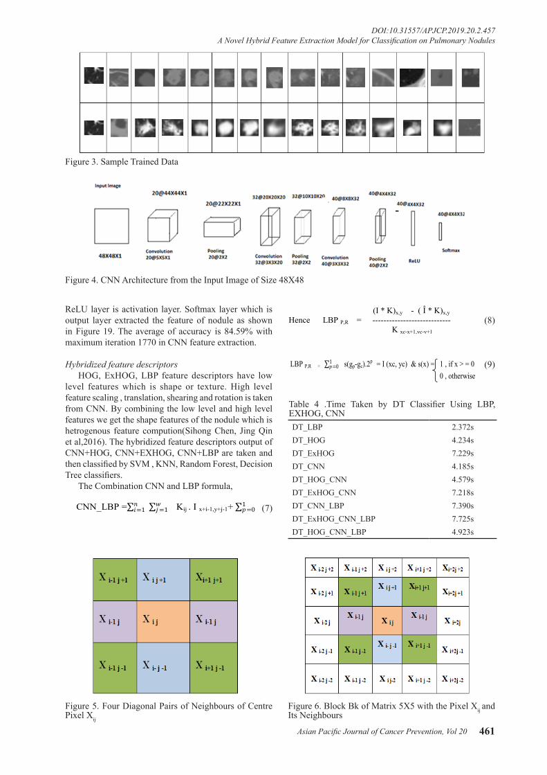
Asian Pacific Journal of Cancer Prevention, Vol 20 461
DOI:10.31557/APJCP.2019.20.2.457A Novel Hybrid Feature Extraction Model for Classification on Pulmonary Nodules
ReLU layer is activation layer. Softmax layer which is output layer extracted the feature of nodule as shown in Figure 19. The average of accuracy is 84.59% with maximum iteration 1770 in CNN feature extraction.
Hybridized feature descriptorsHOG, ExHOG, LBP feature descriptors have low
level features which is shape or texture. High level feature scaling , translation, shearing and rotation is taken from CNN. By combining the low level and high level features we get the shape features of the nodule which is hetrogenous feature compution(Sihong Chen, Jing Qin et al,2016). The hybridized feature descriptors output of CNN+HOG, CNN+EXHOG, CNN+LBP are taken and then classified by SVM , KNN, Random Forest, Decision Tree classifiers.
The Combination CNN and LBP formula, (7)
(8)
(9)
Figure 3. Sample Trained Data
Figure 4. CNN Architecture from the Input Image of Size 48X48
Figure 5. Four Diagonal Pairs of Neighbours of Centre Pixel Xij
Figure 6. Block Bk of Matrix 5X5 with the Pixel Xij and Its Neighbours
DT_LBP 2.372sDT_HOG 4.234sDT_ExHOG 7.229sDT_CNN 4.185sDT_HOG_CNN 4.579sDT_ExHOG_CNN 7.218sDT_CNN_LBP 7.390sDT_ExHOG_CNN_LBP 7.725sDT_HOG_CNN_LBP 4.923s
Table 4 .Time Taken by DT Classifier Using LBP, EXHOG, CNN
CNN_LBP =∑ ∑ 𝑤𝑤𝑗𝑗=1 𝑛𝑛
𝑖𝑖=1 Kij . I x+i-1,y+j-1+ ∑ 1𝑝𝑝=0 s(gp-gc).2p
(I * K)x,y - ( Î * K)x,y
Hence LBP P,R = ---------------------------- (8) K xc-x+1,yc-y+1
LBP P,R = ∑ 1𝑝𝑝=0 s(gp-gc).2p
= I (xc, yc) & s(x) = 1 , if x > = 0 (9) 0 , otherwise

S Piramu Kailasam and M Mohammed Sadik
Asian Pacific Journal of Cancer Prevention, Vol 20462
The hybridized CNN and HOG became as,
(10)
Next HOG and LBP mathematically expressed as,
(11)
(12)
(13)
where LBP of an image can be converted in to
SVM_LBP
SVM_CNN
SVM_EXHOG SVM_HOG SVM_HOG_ CNN
SVM_HOG_ CNN_LBP
SVM_EXHOG_ CNN_LBP
SVM_CNN_LBP
SVM_ EXHOG_ CNN
430 37 429 38 451 16 453 14 453 14 435 32 434 33 453 14 452 1527 104 45 86 26 105 20 111 15 116 24 107 24 107 15 116 13 118
Table 5. Confusion Matrix of SVM Classifier with Other Feature Descriptors
Figure 7. Multi Classifiers with Hybrid Descriptors
RF_LBP RF_CNN RF_EXHOG RF_HOG RF_HOG_ CNN
RF_HOG_ CNN_LBP
RF_EXHOG _CNN_LBP
RF_CNN_LBP
RF_ EXHOG_ CNN
464 3 448 19 466 1 464 3 456 11 435 32 457 10 453 14 456 11
41 90 23 108 55 76 29 102 28 103 24 107 29 102 20 111 33 98
Table 6. Confusion Matrix of Random Forest Classifier with Other Feature Descriptors
Figure 8. HOG - Histogram of Nodule Image
Figure 9. ExHOG-Histogram of Nodule Image
Figure 10. LBP-Histogram of Trained Nodule
(I m,θ * K) x,y=∑ ∑ 𝑤𝑤𝑗𝑗=1 𝑛𝑛
𝑖𝑖=1 Kij . M x+i-1,y+j-1 . 𝑒𝑒𝑖𝑖θ(x+i −1,y+i−1)
I x,y = M(x,y). 𝑒𝑒𝑖𝑖θ(x,y)
LBP = I xc,yc = I M(xc,yc), θ (xc,yc)
LBP = M(xc,yc). 𝑒𝑒𝑖𝑖θ(xc ,yc )

Asian Pacific Journal of Cancer Prevention, Vol 20 463
DOI:10.31557/APJCP.2019.20.2.457A Novel Hybrid Feature Extraction Model for Classification on Pulmonary Nodules
magnitude ‘M’ and angle ‘θ’.
Analysis of classification with different combination of feature descriptors
The Classifiers SVM, K-NN, Decision Tree and Random Forest are used for the classification of nodules and nonnodules. The details of patientid, nodule, noduleid, slicenumber, zposition and diameter are the data collected from LIDC dataset. Here TN and TP values are classified by hyperplane distance in SVM Classifier. All data are tested and trained. Seperate training and test data sets are constructed using k-fold cross validation approach, the
value of k taken as five. In k fold validation 467 nodules and 131 nonnodules are validated and implemented in matlab 2017a. The small round or oval shaped growth in lung size less than or equal to 3mm in diameter is nodule. In the Region of Interest (ROI), the nodule <=3mm assigns the value one or else the value is zero. The nodule intensity is 21 x 21. In CT input dicom images, the nodule region of each five slices taken as p2,p1,n,n1,n2 and trained well. Here ‘n’ is Region of interest. The Positive Predictive Value (PPV) and Negative Predictive Value (NPV) are calculated from confusion matrix. The PPV value of SVM_LBP is 92%. The PPV value of SVM_CNN is
DT_LBP DT_CNN DT_EXHOG DT_HOG DT_HOG_ CNN DT_HOG_CNN_LBP
DT_EXHOG_CNN_LBP
DT_CNN_LBP
DT_ EXHOG_ CNN
424 43 422 45 423 44 422 45 424 43 429 38 417 50 418 49 418 49
31 100 33 98 26 105 27 104 34 97 37 94 35 96 35 96 35 96
Table 7. Confusion Matrix of Decision Tree Classifier with Other Feature Descriptors
KNN_LBP
KNN _CNN
KNN _EXHOG
KNN _HOG
KNN _HOG_ CNN
KNN _HOG_CNN_LBP
KNN _EXHOG_CNN_LBP
KNN _CNN_LBP
KNN _ EXHOG_ CNN
449 18 431 36 451 16 466 1 445 12 449 18 449 18 443 24 451 16
33 98 24 107 24 107 34 97 29 102 33 98 33 98 26 105 24 107
Table 8. Confusion Matrix of KNN Classifier with Other Feature Descriptors
Figure 11. Performance Metrics Analysis of CNN with Classifiers
Figure 12. Performance Metrics Analysis of LBP with Classifiers
Figure 13. Performance Metrics Analysis of HOG with Classifiers
Figure 14. Performance Metrics Analysis of ExHOG With Classifiers

S Piramu Kailasam and M Mohammed Sadik
Asian Pacific Journal of Cancer Prevention, Vol 20464
91.8%, lesser than SVM_LBP. The PPV value of SVM_HOG_CNN, SVM_ExHOG and SVM_HOG_CNN_LBP are 97% ,96.5% and 93% respectively. The NPV value of SVM_LBP is 79.3%. The SVM_CNN, SVM_LBP, SVM_ExHOG, SVM_HOG_CNN_LBP have NPV values as 65.64%, 79.3%, 80.15%, 81.6% vice versa.
The output of hybridized feature descriptors CNN, LBP, HOG, ExHOG combined in various patterns and SVM classifier classified the nodules as shown in Table1 and 2. The results depict that the proposed method
performed well. The TP, TN, FP, FN values are taken from confusion matrix Table1 and Table2. The performance of SVM classifier is calculated using various metrics such as Accuracy, Sensitivity, Specificity, Cohen’s Kappa, Fscore, Precision and Recall. The accuracy of classification based on SVM classifier for both training and test data was evaluated by chi square test at confidence level. The highest accuracy value of SVM_ExHOG_CNN is 95.32% as result. The performances of the SVM Classifier is compared with KNN, Decision Tree and Random Forest
Figure 15. Performance metrics analysis of HOG_CNN with Classifiers
Figure 16. Performance Metrics Analysis of CNN_LBP with Classifiers
Figure 17. Performance Metrics Analysis of ExHOG_CNN with Classifiers
Figure18. Performance Metrics Analysis of EXHOG_CNN_LBP and with Classifiers
Figure 19. The Output Layers of CNN for Given Nnodule

Asian Pacific Journal of Cancer Prevention, Vol 20 465
DOI:10.31557/APJCP.2019.20.2.457A Novel Hybrid Feature Extraction Model for Classification on Pulmonary Nodules
Classifier. The KNN classifier classifies the nodule and nonnodule with K value one and the accuracy 94.15% is obtained. A decision tree is a non-parametric supervised learning method generally used in data mining. The goal is to create a model that predicts the value of target value using decision rules and pruning which inferred from data features. Decision Tree does not work well for simple classification. Random forest uses a number of decision trees in order to improve the classification rate of pulmonary nodule images , depends on the values of a random vector for all trees in the forest. K-NN performs medium level in classification of two classes.
Time Among the determined KNN classifier techniques
minimum time of KNN_LBP is 2.333s which is tabulated and the minimum value is bolded. The DT_LBP gives the time value as 2.37s which is lower than SVM classifier. The RF_LBP gives the time value 11.999s which is higher than the other classifiers.
AccuracyOver all Accuracy value is calculated in the combination
of SVM_LBP, SVM_HOG, SVM_ExHOG, SVM_CNN, SVM_ExHOG_CNN, SVM_CNN_LBP, SVM_HOG_
CNN. The result shows the accuracy value of both SVM_HOG_CNN and SVM_CNN_LBP are the same as 95.15% and the highest accuracy value is SVM_ExHOG_CNN as 95.32%. The value of SVM_ExHOG_CNN value is greater than SVM_HOG, SVM_ExHOG, SVM_CNN, SVM_CNN_LBP, SVM_HOG_CNN combinations. It is noted that SVM classifier is improved in CNN + ExHOG than CNN+HOG . The accuracy value of KNN classifier is good with HOG descriptor as 94.15%. Random forest classifier‘s best accuracy value with HOG is 94.65% and other combinations are greater than 90.64%. Decision Tree classifier with ExHOG combination gives best accuracy value as 88.3%.
(14)
Where TP is true positive that counts classified foreground pixels. FP counts the background pixels incorrectly classified as foreground. FN false negative that counts foreground pixels incorrectly classified as background. TN counts correctly classified background pixels.
SpecificityIt is the ability of the classifier to predict the true
Accuracy = 𝑇𝑇𝑇𝑇+𝑇𝑇𝑇𝑇𝑇𝑇𝑇𝑇+𝐹𝐹𝑇𝑇+𝐹𝐹𝑇𝑇+𝑇𝑇𝑇𝑇
Figure 20. Overall Acuracy
Figure 21. Accuracy Vs Iteration for Proposed Convolutional Neural Network (ConvNet)
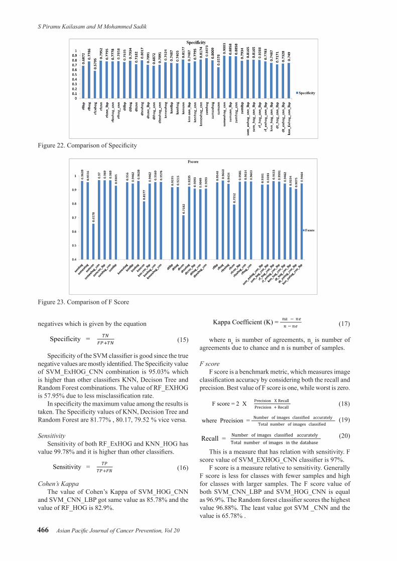
S Piramu Kailasam and M Mohammed Sadik
Asian Pacific Journal of Cancer Prevention, Vol 20466
negatives which is given by the equation
(15)
Specificity of the SVM classifier is good since the true negative values are mostly identified. The Specificity value of SVM_ExHOG_CNN combination is 95.03% which is higher than other classifiers KNN, Decison Tree and Random Forest combinations. The value of RF_EXHOG is 57.95% due to less misclassification rate.
In specificity the maximum value among the results is taken. The Specificity values of KNN, Decision Tree and Random Forest are 81.77% , 80.17, 79.52 % vice versa.
SensitivitySensitivity of both RF_ExHOG and KNN_HOG has
value 99.78% and it is higher than other classifiers.
(16)
Cohen’s KappaThe value of Cohen’s Kappa of SVM_HOG_CNN
and SVM_CNN_LBP got same value as 85.78% and the value of RF_HOG is 82.9%.
(17)
where na is number of agreements, ne is number of agreements due to chance and n is number of samples.
F scoreF score is a benchmark metric, which measures image
classification accuracy by considering both the recall and precision. Best value of F score is one, while worst is zero.
(18)
(19)
(20)
This is a measure that has relation with sensitivity. F score value of SVM_EXHOG_CNN classifier is 97%.
F score is a measure relative to sensitivity. Generally F score is less for classes with fewer samples and high for classes with larger samples. The F score value of both SVM_CNN_LBP and SVM_HOG_CNN is equal as 96.9%. The Random forest classifier scores the highest value 96.88%. The least value got SVM _CNN and the value is 65.78% .
Figure 22. Comparison of Specificity
Figure 23. Comparison of F Score
Specificity = 𝑇𝑇𝑇𝑇𝐹𝐹𝑇𝑇+𝑇𝑇𝑇𝑇
Sensitivity = 𝑇𝑇𝑇𝑇𝑇𝑇𝑇𝑇+𝐹𝐹𝑇𝑇
Kappa Coefficient (K) = 𝑛𝑛𝑛𝑛 − 𝑛𝑛𝑒𝑒𝑛𝑛 − 𝑛𝑛𝑒𝑒
F score = 2 X Precision X RecallPrecision + Recall
where Precision = Number of images classified accuratelyTotal number of images classified
Recall = Number of images classified accuratelyTotal number of images in the database

Asian Pacific Journal of Cancer Prevention, Vol 20 467
DOI:10.31557/APJCP.2019.20.2.457A Novel Hybrid Feature Extraction Model for Classification on Pulmonary Nodules
Discussion
Many researchers used LIDC-IDRI dataset to Classify nodules. A Combination of shape, margin and texture based features for classification pulmonary nodules are segmented using a semi automated technique and classified using SVM classifier to attain accuracy. But Ashis Kumar et al., (2016) is not considered maximum correlation coefficient and provide only seed point for segmentation of nodules. Prajwal et al., (2016) dealed ConNet architecture. ConNet a type of CNN have special properties such as special invariance and allow multiple feature extraction accuracy improvement. ConNet are much better than ANN architecture in accuracy. Qing Zeng et al., (2017) results show that the CNN network achieved the best accuracy of 84.15%. This was the best result among the CNN, DNN and SAE networks. Huan et al., (2010) extracted 14 GLCM textural features to analyze the CT images of benign and malignant pulmonary nodules. The author suggested that need additional variable for explaining texture features in CT images of benign and malignant. He used multilevel binomial logistic prediction model of pulmonary feature of CT images. Goncalves et al., (2016) approaches 3D lung nodule segmentation with Hessian based matrix. He proposed a method validated with 569 solid nodules, provided accurate pulmonary nodule volumes for posterior characters. Shape index and Curvedness approaches are calculated in justavascular nodules. Aranaud et al., (2016) detected multiview convolutional neural network automatically learnt discriminative features from the LIDC data with sensitivities 85.4% at 1 false positive per scan with low computation time to detect nodules. Multitask learning to leverage heterogenous computational features derived from deep learning models of Stacked Denoising Autoencoder (SDAE) and CNN, as well as Hand crafted Haar like and HOG features for the description of a semantic features of lung nodule. The gap between the clinical remark concepts and the low level image features are the major factors that thwarts the retrieval accuracy. The step of computational mapping between the clinical remark terms and image contents to define the similarity measures at semantic level can helped to improve the CBIR performance. In this method the retrieval is based on overall similarity or each specific semantic feature.
In the proposed work, it is observed that the tree based classifiers Decision tree and Random Forest with hybrid feature vectors in deep learning produces lower classification rate ie. approximately 86 – 94 % compared to other classifiers SVM and KNN. Yet SVM can handle the classification of nodules in images well in manner with accuracy rate 95.32%. KNN is also having accuracy as 94.15%. It is noticed that SVM (RBF kernel) can be appropriate classifier for large datasets.
In conclusion, in Deep learning environment, the proposed hybridized feature descriptor is found to be the best for LIDC pulmonary image dataset. This paper presents the test results of classification of the pulmonary image dataset. The feature descriptors CNN, LBP, HOG, ExHOG are hybridized in two or three combinations with various single classifiers that is like SVM, KNN, DT
and RF. It may be noted that the SVM_CNN_LBP and SVM_HOG_CNN have classification accuracy which is comparable to the accuracy value of SVM_EXHOG_CNN and the accuracy is 95.15%. SVM_EXHOG_CNN assists in achieving the highest classification accuracy of 95.32% and the execution time is 3s more than KNN_LBP’s execution time 2.233s. Therefore SVM_EXHOG_CNN is 10.04% higher than DT_HOG_CNN in terms of accuracy. Among 36 combinations tried the execution time of KNN_LBP got to be the least with value 2.233s. Considering all the above points, SVM classifier is better than KNN, DT and RF classifiers for the classification of two classes due to its higher accuracy. In future best detection of malignant lung nodule can be achieved by training 2DCNN to 3DCNN with other datasets.
Referrences
Alif Hayat M (2015). Classification of membrane protein types using voting feature interval in combination with Choo’s pseudo amino acid composition. Theor Biol, 384, 78-83.
Amit S, Xudong J, How-Lung E (2011). Extended histogram of gradients with asymmetric principal component and discriminant analyses for human detection. IEEE Canadian Conference on Computer and Robot Vision, pp 64-71.
Ani Brown Mary N, Dejey D (2017). Coral reef image classification employing Improved LDP or feature extraction. IVCIR, 49, 225-42
Apte C, Weiss SM (1997). Data mining with decision trees and decision rules. Future Gener Comput Syst, 13, 197-210.
ArmatoSG,McLennan G, Bidaut L (2011). The lung image database consortium (LIDC) and image database resource initiative (IDRI), a completed reference database of lung nodules on CT scans. Med Phys, 38, 915-31
Ashis kumar D, Sudipta M, Anirvan D, Mandeep G, Niranjan K (2016). A combination of shape and texture features for classification of pulmonary nodules in lung CT images. Springer, 29, 466-75.
Beijbom O, Edmunds PJ, Kline DI, Mitchell BG, Krigman D (2012). Automated annotation of coral reef survey images,in: Proceedings of IEEE conference on computer vision and pattern recognition (CVPR), providence, Rhode Island, pp 16-21.
Chen J, Chen Z, Ch Z, Fu H (2014). Facial expression recognition based on facial components detection and Hog features. in international workshops on ECE sub fields, pp 884-8.
Corinna C,Vladimir V (1995). Support vector networks.Machnine Learning, 20, 273-97.
Eduardo T, Alan R, David ML, Hyxia V, Antonio B (2014).Implementation of a fast coral detector using a supervised machine learning and gabor wavelet feature descriptors, Sensor Systems for a Changing Ocean (SSCO). IEEE, pp1-6.
Golmohammadi KSK, Crowley L, Reformat M (2007). Classification of cell mem- brane proteins. Front Convergence Biosci Inf Technol, 20, 153 -8.
Goncalves L, Novo J (2016). A. Canpilho, Hessian based approaches for 3D lung nodule segmentation. Exp Sys Appl, 61, 1-15.
Gould MK, Donington J (2013). Evaluation of individuals with pulmonary nodules: When is it lung cancer?: Diagnosis and management of lung cancer: American College of Chest Physicians evidence-based clinical practice guidelines. Chest, 143, 93 –120.
Hayat M, Khan A (2012a). Mem- PHybrid: hybrid features-based prediction system for classifying membrane protein types.

S Piramu Kailasam and M Mohammed Sadik
Asian Pacific Journal of Cancer Prevention, Vol 20468
Anal Biochem, 424, 35 -44He Y, Hengyong Yu (2016). Deep learning for the classification
of lung nodules, Conference Paper, Cornell University.Huan W, Xiu H, Zhong WJ, et al (2010). Multilevel binomial
logistic prediction model for malignant pulmonary nodules based on texture features of CT image. Eur J Radiol, 74, 124-9.
Jie-Zhi C, Dong N, Yi-Hong C, et al (2016). Computer aided diagnosis with deep learning architecture:Applications to breast lesions in US images and pulmonary nodules in CT scans. Sci Rep, 6, 1-13
McWilliams A, Martin MB,Tammemagi C, et al (2013). Probability of cancer in pulmonary nodules detected on first screening CT. N Engl J Med, 369, 910-9.
Niranjana G, Ponnavaikko M (2017). A review on image processing methods in detecting lung cancer using CT images. International Conference on Technical Advancements in Computers and Communications, pp10-1.
Prajwal R, Nishal A, Perieira RS (2016). Convolutional neural networks for lung cancer screening in computed tomography (CT)scans. IEEE, DOI:10.1109/IC3I.2016.7918014.
Qi D, Hao C, Lequan YU, et al(2016). Multi-level contextual 3D CNNs for false positive reduction in pulmonary nodule detection. Biomed Eng, 64, 1558-67.
Qingzeng S, Lei Z, Xcing Ke L, Xuechen D (2017). Using deep learning for classification of lung nodules on Computed tomography images. J Health Care Eng, 2017, 7.
Rabia N, Khurram SA, Tariq B (2017). Recent trends in Computer Aided diagnosis of lung nodules in thorax CT scans. International Conference on Innovations in Electrical EngineeringAnd Computational Technologies, pp 5-7.
Rangayyan RM, El-Faramwy NM, Desautel JL, Alim OA (1997).Measures of acutance and shape for classification of breast tumors. IEEE Trans Med Imaging, 16, 799 -810.
Sihong C, Jing Q ,Xing J (2016). Automatic scoring of multiple semantic attributes with multi-task feature leverage: A study on pulmonary nodules in CT images. IEEE, 36, 802-14.
Tara NS, Abdel - Rahman M, Brian K, Bhuvana R(2013), Deep donvolutional neural of networks for LVCSR. IEEE conference,Speech and signal processing, DOI:10.1109/ICASSP.2013.6639347.
Vishal KP, Sagar KN, David PN, et al (2013). A practical algorithmic approach to the diagnosis and management of solitary pulmonary nodules. Chest J, 143, 840-6.
This work is licensed under a Creative Commons Attribution-Non Commercial 4.0 International License.

Abstract—This study is expected to compress true color image
with compression algorithms in color spaces to provide high compression rates. The need of high compression ratio is to improve storage space. Alternative aim is to rank compression algorithms in a suitable color space. The dataset is sequence of true color images with size 128 x 128. HAAR Wavelet is one of the famous wavelet transforms, has great potential and maintains image quality of color images. HAAR wavelet Transform using Set Partitioning in Hierarchical Trees (SPIHT) algorithm with different color spaces framework is applied to compress sequence of images with angles. Embedded Zerotrees of Wavelet (EZW) is a powerful standard method to sequence data. Hence the proposed compression frame work of HAAR wavelet, xyz color space, morphological gradient and applied image with EZW compression, obtained improvement to other methods, in terms of Compression Ratio, Mean Square Error, Peak Signal Noise Ratio and Bits Per Pixel quality measures.
Keywords—Color Spaces, HAAR Wavelet, Morphological
Gradient, Embedded Zerotrees Wavelet Compression.
I. INTRODUCTION
ECENT techniques in the discipline of image analysis resulted large amount of images in each time. Processed
image or video takes large storage area during the time of download or upload. Similarly, the storage and transmission of statistics is big hassle and there is a necessity to take essential steps. As stated by way of Parkirson’s first law [13], as the necessity of storage increases, transmission capacity twice will increase. Though it is far boom in rate, the storage capacity is good than the technology. Data compression deals with morse code later hired in the famous Huffman code. In order to overcome this challenge, data compression [17] has been presented to compress the size of data being stored or transmitted. Eliminating redundancies is subsequent state of artwork method to symbolize information in binary form. The velocity of moving records rate in WIFI is becoming important these days because of thousands and thousands of users in social media. The storage and computation speed are not in direct percentage. Like sparse matrix, the redundant records are compressed by suitable compression algorithms like EZW, SPIHT, Spatial Orientation Tree Wavelet (STW), Wavelet Difference Reduction (WDR), Adaptively Scanned Wavelet Difference Reduction (ASWDR) and SPIHT 3-D.
II. RELATED WORKS
In this section existing papers applied inside the discipline of image compression are explained elegantly. The wavelet
S. Piramu Kailasam is Assistant Professor with Sadakathullah Appa College, India (e-mail: [email protected]).
remodel [5] has important role with image compression. The wavelet is outstanding than Discrete Cosine Transform (DCT) [10]. Similarly, wavelet based compression is best in interpreting mistakes and transmission of images because of the purpose of high resolution nature [7] and degradation tolerance. In [1], the Huber–Markov random field model with objective artifact achieved good Bits per pixel (BPP) and PSNR.
Alzahir and Borici [4] compress discrete color images used the method codebook row column reduction coding in comparison with maps and binary images.
Babu et al. [2] overcome the drawback of Run Length Coding (RLC) with matrix based on mapped-pair approach. In addition, the author analysed the performance metric of compressed images .tiff, .jpg, .gif and text documents by RMSE, SNR, PSNR and CR. The robustness and compression efficiency [9] is performed in lossless compression [2] technique for color images and raster images. Consequently, DCT area has been introduced in most video compression techniques [2]. The overall performance of DCT degrades in high compression ratio [14]. Moreover, many researchers substantially target Discrete wavelet transform (DWT). DWT [14] is appropriate for human visible gadget for purpose of adaptive spatial frequency. At the same time, another compression algorithm, Embedded zerotree, does no longer need preknowledge of image. EZW is good enough in encoding and accuracy rate for true color images.
In embedded image coding, the usage of zerotree of wavelet coefficient (EZW) using stream of bits [6] is an efficient lossy compression image technique. Larger coefficients of EZW are the prime factors than smaller coefficients regardless of their scale [16]. An embedded code is produced in the order of importance. It defines a string of binary selections. In EZW, encoding and decoding may be ended when the goal is reached. EZW [17] is the basic method for tree shape approach and it is an effective embedded image compression that generates bit circulation. Ultimately SPIHT [11] is refinement to EZW and it uses the principle of operation. Evaluation of EZW, SPIHT is high in terms of compression parameter [12]. In alternative, SPIHT coding operates in exclusive scales on the equal spatial vicinity within the wavelet subbands. This yields embedded bits with less MSE. Similarly, SPIHT can be useful to lossless algorithm [15].
Jamel [21] pointed that SPIHT algorithm is simple computation approach. The work in SPIHT algorithm [18] suggests that the execution time is reduced when compression ratio value is elevated. DWT-SPIHT is good in quality with high PSNR. The wavelet based contourlet transform (WBCT)
Efficient HAAR Wavelet Transform with Embedded Zerotrees of Wavelet Compression for Color Images
S. Piramu Kailasam
R
World Academy of Science, Engineering and TechnologyInternational Journal of Computer and Information Engineering
Vol:14, No:11, 2020
406International Scholarly and Scientific Research & Innovation 14(11) 2020 ISNI:0000000091950263
Ope
n Sc
ienc
e In
dex,
Com
pute
r an
d In
form
atio
n E
ngin
eeri
ng V
ol:1
4, N
o:11
, 202
0 pu
blic
atio
ns.w
aset
.org
/100
1157
7/pd
f

using SPIHT like algorithm is visually superior to the wavelet SPIHT in preserving data and texture details.
Ajala et al. worked on hybrid compression. The LZW and Huffman image compression strategies are helped to broaden hybrid compression [1] in clinical images. Concatenation of LZW code words and Huffman blunders detection techniques are implemented to get size reduction, high compression ratio and high signal noise ratio.
SPIHT algorithm is a powerful wavelet based image compression algorithm, here the tree structure is chosen to represent the transformed image which is identified by the coefficients of each node. The existing work focused that Runlength Encoding [17] employs high redundant data in loss less compression. Pearlman pointed that SPIHT [15] method is efficient for wavelet image compression [3]. SPHIT uses arithmetic coding to improvise image quality and it is suitable for hardware implementations. Later days SPIHT has become benchmark algorithm. It is one of the best wavelet based coding algorithms. 3D SPIHT coding is an excellent technique to color image compression than conventional methods such as EZW; SPIHT always generates local optimal values. 3D SPIHT [11], [19] is the modern octal tree technique for 3 dimensional true color image compression. In this study 3D SPIHT with different color conversion methods are applied to different types of images. SPHIT algorithm is applied to sequence of images with consequent angles. It is experimented with true color image as well as gray scale image.
The LZW and Run length Encoding compression methods are excellent to Tiff documents. Especially LZW is suitable for textual content files. Another technique LVL_MMC (subband thresholding of coefficients and Huffman Encoding) is a level thresholding wavelet compression method. The parameters of this subband thresholding are calculated from the differences between means method. One of the most important papers on image compression within 1977, by Ziv and Lempel notably pointed about compression with all varieties of facts. In the paper [20], LZ coding, dictionary based coding with loss much, less strategies are applied on Tiff, Gif, Pdf, Gzip, Zip, V.42 and Png files.
III. MATERIAL AND METHOD
A sequence of portable network graphics (png) file formats are taken as input images. This image contains a single or multi image in an extensible structure of chunks, encoding with the basic pixels and other textual information. The file size is 128x128.
A. Color Space Based Compression Algorithm
In this observation, the three goals are as follows: The first objective is to discover best color space with
HAAR wavelet based compression techniques EZW, SPHIT, SPIHT 3D, LVL-MMC using true color images.
The second objective is to find best compression method for sequence of true color images as well as gray color images for best compression ratio.
The third objective is applying morphological gradient input image to get best compression ratio and PSNR using
proposed frame work.
Fig. 1 Sample True Color Images The motive of this work is to lessen the storage area and
improve compression ratio using HAAR wavelet compression approach. The proposed work is dealt with series of images with .png files. Further the file formats png, bmp, tiff files are checked using color space conversion techniques rgb, yuv, kit, yiq and xyz. Here yuv represents YUV colour space transform, klt represents Karhunen-Loeve transform, yiq represents YIQ color space transform, xyz represents CIE-XYZ color space transform. XYZ color space transform gives suitable for true color single object image.
There are legitimate compression strategies which can be progressive coefficients significance method (PCSM) and Coefficient thresholding method. Embedded zerotree wavelet, SPIHT, Spatial Orientation Tree, wavelet difference reduction, Adaptively Scanned Wavelet difference reduction, SPIHT 3-D are the compression techniques comes beneath PCSM category. Among these compression techniques the proposed work uses EZW, SPHIT, SPHIT 3-D and LVL-MMC methods which are suitable for png type single object files.
On this segment, the technique for assessing reconstruction and overall performance of HAAR wavelet for compressing unique record codecs has been investigated using MATLAB. To schematic diagram of experiment is shown in Fig. 2. During the evaluation period EZW, SPIHT, SPIHT 3-D, LVL-MMC are examined for gray scale and true color single object sequence images. Also same strategies are tried to Tiff, Bmp, Jpg, Png file formats. The Compression ratio, PSNR and Saving space % measure the reconstruction performance of an image. Here compression ratio represents compressed image in terms of storage. PSNR represents maximum pixel magnitude of original image.
B. Morphological Gradient
In order to achieve good PSNR and compression ratio, morphological internal gradient method is applied. This internal gradient (Gi) operation forms edge enhanced image with 3x3, 6x6, 12x12 in x, y axes. Transitions of image edges’
World Academy of Science, Engineering and TechnologyInternational Journal of Computer and Information Engineering
Vol:14, No:11, 2020
407International Scholarly and Scientific Research & Innovation 14(11) 2020 ISNI:0000000091950263
Ope
n Sc
ienc
e In
dex,
Com
pute
r an
d In
form
atio
n E
ngin
eeri
ng V
ol:1
4, N
o:11
, 202
0 pu
blic
atio
ns.w
aset
.org
/100
1157
7/pd
f

representation from dark to bright and bright to dark region in morphological gradient’s procedure is as: Step1. Create a duplicate of the input image. Let it be Q. Step2. Apply Erosion operation to the input image (P). Step3. Edge = Input Image – Eroded Image,
i.e., Gi = P - (P Ɵ Q) Step4. Display the Gradient image Step5. Exit
Here image may be either True Color Image or Gray Scale Image.
IV. RESULT AND DISCUSSION
The SPIHT algorithm gives good PSNR value and the values are plotted as graph below. Fig. 3 shows that when the angle increases from 5 to 85 degree the PSNR value decreases. When the angle reached at 90 degree the curve goes down. In addition, at the angle of 90 to 160 degree the PSNR values are in increasing order for gray scale image as shown in Fig. 3.
Fig. 2 Schematic Diagram
Fig. 3 PSNR attained for Gray Scale image
Fig. 4 MSE attained for Gray Scale Image
Fig. 4 shows that the MSE value of gray scale images slowly increase from the angle 5 to 80 degrees and suddenly
Image
Apply Compression
Methods (EZW, SPIHT,
SPIHT 3D, LVL-MMC)
Apply HAAR Wavelet, Morphological gradient
Apply Color Spaces to True
Color Image and Gray Color Image
Apply Best Color Spaces Select Best Compression Method
Reconstruct Image with Best Color Space and Compression method
World Academy of Science, Engineering and TechnologyInternational Journal of Computer and Information Engineering
Vol:14, No:11, 2020
408International Scholarly and Scientific Research & Innovation 14(11) 2020 ISNI:0000000091950263
Ope
n Sc
ienc
e In
dex,
Com
pute
r an
d In
form
atio
n E
ngin
eeri
ng V
ol:1
4, N
o:11
, 202
0 pu
blic
atio
ns.w
aset
.org
/100
1157
7/pd
f

increase from the angle 20 to 70. Along with this, there is decrement in angle from 70 to 25 then it slowly decreases from 100 to 160 degree. True color image’s MSE value is higher than gray scale image in SPIHT method.
In SPIHT method, the compression ratio is lesser in true color images than gray scale images. Fig. 4 shows that compression ratio also displays the result similar to PSNR graph, Fig. 3.
Fig. 5 Space Saving for True Color Image
Even though the lossy EZW coding algorithm reduces number of bits, still it cannot compromise loss of information.
SpaceSaving=1 -
(1)
Space saving is a second quality measure compression
method using compression ratio. This gives the numerical value of storage space saved by the HAAR-EZW method. Equation (1) shows the unity difference of ratio between number of bits in compressed data and uncompressed data gives the storage value of SpaceSaving.
The SPIHT algorithm has been applied to true color images. The notable point is that PSNR values received from true color images using SPHIT are greater than gray color with SPIHT method.
Fig. 6 Comparison of PSNR and BPP for True Color Image
Fig. 7 Sample compressed gray scale images of SPIHT Method and true color images O1,O2,O3,O4,O5
In order to achieve good PSNR and compression ratio,
morphological internal gradient method is applied. Fig. 8 shows the results for test gray scale images. The
LVL-MMC compression method is driven by morphological gradient to increase PSNR value. The results of true color
Angle Vs Space Saving
0 20 40 60 80 100 120 140 16085
86
87
88
89
90
91
92
Sp
ace
Sa
vin
g %
Angle
World Academy of Science, Engineering and TechnologyInternational Journal of Computer and Information Engineering
Vol:14, No:11, 2020
409International Scholarly and Scientific Research & Innovation 14(11) 2020 ISNI:0000000091950263
Ope
n Sc
ienc
e In
dex,
Com
pute
r an
d In
form
atio
n E
ngin
eeri
ng V
ol:1
4, N
o:11
, 202
0 pu
blic
atio
ns.w
aset
.org
/100
1157
7/pd
f
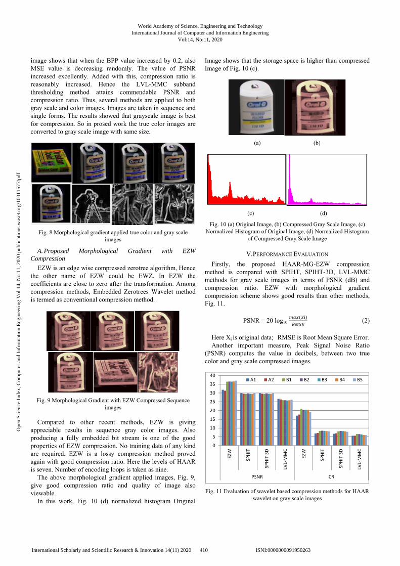
image shows that when the BPP value increased by 0.2, also MSE value is decreasing randomly. The value of PSNR increased excellently. Added with this, compression ratio is reasonably increased. Hence the LVL-MMC subband thresholding method attains commendable PSNR and compression ratio. Thus, several methods are applied to both gray scale and color images. Images are taken in sequence and single forms. The results showed that grayscale image is best for compression. So in prosed work the true color images are converted to gray scale image with same size.
Fig. 8 Morphological gradient applied true color and gray scale images
A. Proposed Morphological Gradient with EZW Compression
EZW is an edge wise compressed zerotree algorithm, Hence the other name of EZW could be EWZ. In EZW the coefficients are close to zero after the transformation. Among compression methods, Embedded Zerotrees Wavelet method is termed as conventional compression method.
Fig. 9 Morphological Gradient with EZW Compressed Sequence images
Compared to other recent methods, EZW is giving
appreciable results in sequence gray color images. Also producing a fully embedded bit stream is one of the good properties of EZW compression. No training data of any kind are required. EZW is a lossy compression method proved again with good compression ratio. Here the levels of HAAR is seven. Number of encoding loops is taken as nine.
The above morphological gradient applied images, Fig. 9, give good compression ratio and quality of image also viewable.
In this work, Fig. 10 (d) normalized histogram Original
Image shows that the storage space is higher than compressed Image of Fig. 10 (c).
(a) (b)
(c) (d)
Fig. 10 (a) Original Image, (b) Compressed Gray Scale Image, (c) Normalized Histogram of Original Image, (d) Normalized Histogram
of Compressed Gray Scale Image
V. PERFORMANCE EVALUATION
Firstly, the proposed HAAR-MG-EZW compression method is compared with SPIHT, SPIHT-3D, LVL-MMC methods for gray scale images in terms of PSNR (dB) and compression ratio. EZW with morphological gradient compression scheme shows good results than other methods, Fig. 11.
PSNR = 20 log10 (2)
Here Xi is original data; RMSE is Root Mean Square Error. Another important measure, Peak Signal Noise Ratio
(PSNR) computes the value in decibels, between two true color and gray scale compressed images.
Fig. 11 Evaluation of wavelet based compression methods for HAAR wavelet on gray scale images
0
5
10
15
20
25
30
35
40
EZW
SPHIT
SPHIT 3D
LVL‐MMC
EZW
SPHIT
SPHIT 3D
LVL‐MMC
PSNR CR
A1 A2 B1 B2 B3 B4 B5
World Academy of Science, Engineering and TechnologyInternational Journal of Computer and Information Engineering
Vol:14, No:11, 2020
410International Scholarly and Scientific Research & Innovation 14(11) 2020 ISNI:0000000091950263
Ope
n Sc
ienc
e In
dex,
Com
pute
r an
d In
form
atio
n E
ngin
eeri
ng V
ol:1
4, N
o:11
, 202
0 pu
blic
atio
ns.w
aset
.org
/100
1157
7/pd
f

The most popular measure to calculate efficiency of a compression algorithm is compression ratio (CR). It is defined as the ratio of bits to store uncompressed data and total number of bits to store compressed data.
CR =
(3)
Secondly the HAAR-MG-EZW scheme is compared in
terms of BPP for all test images as Fig. 12. EZW-BPP value is 1.67. Hence for true color image, BPP ratio is 24:1.67. This is notably high than other methods. But, the smallest BPP value is 0.45 for LVL-MMC method and BPP ratio is 24:0.45. Here, BPP is an absolute value which represents the average number of bits needed to encode the image pixel information with HAAR-MG-EZW compression scheme.
Fig. 12 Bits Per Pixel attained for test images
In Fig. 12, A1, A2, B1, B2, B3, B4, B5 are gray scale sequence images as per Fig. 7.
MSE = ∑ Xi – Yi 2 (4)
Here Xi is original data, Yi is reconstructed data.
TABLE I
MSE FOR SEQUENCE OF GRAY SCALE IMAGES
IMAGES HAAR-
MG-EZW HAAR-MG-
SPIHT HAAR-MG-SPIHT 3D
HAAR-MG-LVL_MMC
O1 14.72 73.94 73.94 168.5
O2 14.31 69.04 69.07 167.8
O3 14.67 72.62 72.62 173.4
O4 14.24 73.81 73.81 169.9
O5 12.90 64.90 64.90 156.0
CR% FOR SEQUENCE OF GRAY SCALE IMAGES
IMAGES HAAR-
MG-EZW HAAR-MG-
SPIHT HAAR-MG-SPIHT 3D
HAAR-MG-LVL_MMC
O1 20.92 8.36 8.15 6.6
O2 20.27 8.5 8.34 6.54
O3 20.43 8.39 8.26 6.34
O4 20.39 8.29 8.13 6.06
O5 19.09 8.07 7.87 6
The Mean Square Error is used to compare the image quality. This work gives the result such that when the MSE value is low then the quality of compressed image is high. Table I depicts that HAAR-MG-EZW method gives the lowest MSE value 12.90. HAAR-MG-LVL-MMC method shows the highest error value 173.4.
Compression Ratio percentage of EZW is higher than SPIHT, SPIHT-3D AND LVL_MMC methods. In this work, the results of YUV and YIQ color space methods gave high MSE values whereas, KIT and XYZ methods showed low MSE and Max Error values.
VI. CONCLUSION
Image compression is one of the exceptional applications of data compression to lessen information redundancy in an efficaciously way. Image Reconstruction in overall performance of HAAR Wavelet is vital due to the fact that series of coefficients are used for extraordinary instance of time. The exceptional choice of color space xyz using png image is implemented to series images and different file formats with varying dimensions also evaluated. The end result confirmed that HAAR wavelet method is comparatively faster and much less complexity than other wavelet methods. Experimental effects additionally show that HAAR-EZW is satisfactory in compression ratio. The image satisfactory is relying on the image type and compression ratio. This study confirms that high compression ratio produces low image quality. HAAR_LVL_MMC is good in PSNR value. In consequent sequence image using SPIHT is the best technique in phrases of compression errors and compression ratio.
REFERENCES [1] Ajala F.A., Adigun A.A, Oke A.O, ”Development of Hybrid
Compression Algorithm for Medical Images using Lempel-Ziv-Welch and Huffman Encoding”, IJRTE,Vol.7, 2018
[2] Anantha Babu, S., Eswaran, P., Senthil Kumar, C., “Lossless compression algorithm using improved RLC for grayscale image”, Arab. J. Sci. Eng. 41, 3061–3070. https://doi.org/10.1007/s13369-016-2082-x., 2016
[3] Ali Kadhim, Al-Janabi, ”Efficient and simple scalable image compression algorithms”, Ain Shams Engineering Journal,vol.10,463-470 (wavelet image compression),2019
[4] Alzahir, S., Borici, A., “An innovative lossless compression method for discrete color Images”, IEEE Trans. Image Process. 24, 44–56,2015
[5] Gonzalez R and Wood R, "Digital image processing. 2nd Edition, Pearson Education Inc., London, England. 2002
[6] Jerome, S.,119.pdf,1993 [7] Kang LW, Hsu CC, Zhuang B, Lin CW, and Yeh CH, “Learning-based
joint super-resolution and deblocking for a highly compressed image”, IEEE Transactions on Multimedia, 17(7), 2015, 921-934.
[8] Kim BJ , Pearlman WA , “An embedded wavelet video coder using three dimensional set partitioning in hierarchical trees (3D-SPIHT)”, In the Proceeding of Data Compression Conference 1997, Snowbird, Utah, USA:,1997, 251−260.
[9] Khan. A, Khan. A., Khan. M, Uzir. M, “Lossless Image Compression: application of bi-level burrows wheeler compression algorithm (BBWCA) to 2d data”, Multimedia Tools Application,2016
[10] Luo, J., Chen, C.W., Parker, K.J., Huang, T.S., “Artifact reduction in low bit rate DCT-based image compression”, IEEE Trans. Image Process. 5, 1363–1368,1996
[11] Mohammed Pooyan, Ali Taheri, “Wavelet Compression of ECG Signals Using SPIHT Algorithm”, International Journal of Signal Processing, 2004
[12] S. Nirmalraj, “SPIHT: A Set Partitioning in Hierarchical Trees
0
0,2
0,4
0,6
0,8
1
1,2
1,4
1,6
1,8
A1 A2 B1 B2 B3 B4 B5
BPP EZW BPP SPHIT BPP SPHIT 3D BPP LVL‐MMC
World Academy of Science, Engineering and TechnologyInternational Journal of Computer and Information Engineering
Vol:14, No:11, 2020
411International Scholarly and Scientific Research & Innovation 14(11) 2020 ISNI:0000000091950263
Ope
n Sc
ienc
e In
dex,
Com
pute
r an
d In
form
atio
n E
ngin
eeri
ng V
ol:1
4, N
o:11
, 202
0 pu
blic
atio
ns.w
aset
.org
/100
1157
7/pd
f

Algorithm for Image Compression”, Contemporary Engineering Sciences, Vol.8, 2015, 263-270.
[13] Parkinson, C.N., “Park Parkinson’s First Law: Work expands so as to fill the time available.” In: Parkinson’s Law and Other Studies in Administration, Ballantine Books, New York,1957
[14] Ranjeet Kumar, Utpreksh Patbhaje, A. Kumar, (2019). “An efficient technique for image compression and quality retrieval using matrix completion”, Journal of King Saud University Computer and Information sciences,2019
[15] A. Said and W. A. Pearlman, (1996). “A New Fast and Efficient Image Codec Based on Set Partitioning in Hierarchical Trees,” IEEE trans. On Circuits and Systems for Video Technology, vol. 6, 1996, pp. 243-250
[16] J.M. Shapiro, “Embedded image coding using zerotrees of wavelet coefficients,” IEEE trans. on Signal Processing (Special Issue, Wavelets and Signal Processing), vol. 41,1993, pp. 3445-3462
[17] J. Udhayakumar, T. Vengattaraman, P. Dhavachelvan, “A Survey on Data Compression techniques: from the perspective of data quality, coding schemes, data type and applications”, Journal of King Saud University- Computer and Information Sciences, 2018.
[18] Vijayakumar Sajjan, Mohammed Parvez Ali, “Design and Implementation of SPIHT algorithm for Image Compression”, IJESC, 2017.
[19] M.R. Zala, S.S. Parmar, “3D Wavelet transform with SPIHT algorithm for image compression”, IJAIEM, 2013.
[20] Ziv, J., Lempel, A., “A universal algorithm for data compression”, IEEE Trans. Inf. Theory 23, 1977, 337–343.
[21] Enas M.Jamel, “Efficiency Spiht in compression and quality of image”, J. of college education for women, vol. 22,2011.
World Academy of Science, Engineering and TechnologyInternational Journal of Computer and Information Engineering
Vol:14, No:11, 2020
412International Scholarly and Scientific Research & Innovation 14(11) 2020 ISNI:0000000091950263
Ope
n Sc
ienc
e In
dex,
Com
pute
r an
d In
form
atio
n E
ngin
eeri
ng V
ol:1
4, N
o:11
, 202
0 pu
blic
atio
ns.w
aset
.org
/100
1157
7/pd
f
Pixel level Image Fusion using Wavelet decomposition technique in Color Images
Mrs. Dr. S. Piramu Kailasam
Assistant Professor
Department of Computer Applications
Sadakthullah appa college(autonomous)
Tirunelveli, India.
Abstract Color Image Fusion is the design method to improve the image substance
by fusing images. The aim of the image fusion is to fuse more useful information and
remove the outliers from registered images. Pixel level Wavelet Image fusion method
is suitable for color images of equal in size as well as resolution in visual perspective.
Quantitative analysis is done using RMSE and entropy, DFE, SSE and R-square
measurements. The analysis report obtained from various image file types give
better result for inverse discrete wavelet transform applied image fusion method.
Keywords Image Fusion · Pixel level Image Fusion · Color Images ·
Wavelet Image Fusion · Resolution
1 Introduction
The use of colour in image processing is given by two principal factors. First the
color is an effective descriptor which is often identify the objects. Secondly, the
manual analysis made by human beings. The colour image processing is classified
into two major areas full color and pseudo colour processing. The result of full color
image processing are now used in visualization and internet. Digital color image
processing is done in pseudo color level. Colour Image fusion is especially useful in
security level in authendicated communication via fast network services. In defence
section, the send images hide with encoded colours in Lab , YCMk color model.
This will be retrieved by applying certain algorithms in terms of DWT technique.
The probability of interception get by inversing number of images to be fused and
the total possibility of combinations of fused images[7] over input images is NCr.
Here N is number of images and r is required images for combination.
The important thing is both the input images should be in same size and
resolution. In color image fusion the image splitted in to R, G, B colors calculated
in bravery color normalized technique by
Rnew=R/(R+G+B) x Pan1 (1)
Gnew=G/(R+G+B)xPan2 (2)
Bnew=B/(R+G+B) x Pan3 (3)
R-Red G-Green B-Blue Pan – Pan image
Mukt Shabd Journal
Volume IX, Issue X, OCTOBER/2020
ISSN NO : 2347-3150
Page No : 860

2 Related works
A multifocus image fusion [5] using SWT and Content adaptive blurring worked
by Fapasmin Sahoo et al., 2018. It combines multiple images of the same
scene with different resolution , intensity to get improved image fusion. Suggested
process conserves the spectral characteristics of the resultant uniformly focused fused
images. The author says the low the value of deviation index is credited. Correlation
coefficient measures the similarity between two images [1].
Fusion rule is formed based upon content adaptive blurring. In another
paper deals the image fusion of under water objects using DWT and SWT to
enhancing the resolution of image rerichment [3]. Discrete wavelet transforms
based image fusion [ 2,11,12] and denoising in FPGA by A. Anoopsuraj , Mathew
fransis (2014) is found by the parameters edge strength , fusion factor, fusion
symmetry using UWT and DTCWT methods [ 2 ]. The sobel edge method gives the
higher edge strength values represents higher edge information. Fusion factor says the
mutual information between source images and fused images. Higher the value
represents better data density. But in the case of fusion symmetry lower the value of
Fusion symmetry better result of image fusion[6].
The novel color image fusion for multi sensor night vision images, the
author says the visible image fused with Infrared image scaling factor is introduced
in transferring equation in the ‘ b ’ channel which gives multiband fused images with
natural day time color appearance.
3 Materials and methods
Image security algorithm using DWT , subband exchange based color image
fusion scheme is developed for enhanced security. Fusion rule [1] can be formed by
following pattern ( min, min ), ( min, max ), ( max, min ), ( min, mean), ( mean,min ),
( mean,median ), ( median,max ), ( median,min ),( max,mean). Fusion rules depend
on fusion application. Image fusion can give better result by choosing best fusion
rule. Fusion also having subtypes updown fusion,downup fusion, rightleft
fusion,right left fusion, user defined fusion and triangular fusion in linear.
Fig.3.1 a. Blur image1 b.Blur image2 c. Original Image (128X128)
Mukt Shabd Journal
Volume IX, Issue X, OCTOBER/2020
ISSN NO : 2347-3150
Page No : 861

IMAGE A (128X128)
IMAGE B (128X128)
DWT DWT
FUSED IMAGE
Color image processing is motivated by color descriptor and color
intensities. Color intensities are important in image analysis. Further color image
processing divided into two sub categories which are full color and pseudo color
processing. The problem of second one is assigning a color to particular intensity or
range of intensities. Color spectrum seen by passing whitelight through prism will
give VIBGR colors. If the light is achromatic then that is called its intensity. The
primary colors are R,G,B. The primary colors can be added to produce secondary
colors of light magenta, cyan and yellow. Distinguish on color from another are
brightness, hue and saturation.
Hue and saturation are called chromaticity. So every color is characterized
by tristimulus values denoted by x,y and z.
x + y + z = 1 here x, y, z are red, green and blue (4)
The types of color models normally used are RGB model, CMYK color model
and HSI color model. Pseudo color or false color image processing is another
milestone, consists of assigning color to gray values. Funtionals FR, FG, FB are fed
into the corresponding red, green and blue inputs of an RGB color monitor for
color image. The f( x,y ) is transformed into 3 colors R,G & B. Hence the output
functions are fR (x,y), fG (x,y), fB (x,y). The color transformations are further
categorize in to RGB-HSI, HSI-RGB conversions. Color complements are hues
opposite to one another on color circle. Color slicing is useful in separating objects
from their surroundings. Histogram processing transformation can be used to
improve color images in another way. Uniform histogram of intensity values method
is alternative type highly suitable for HSI color space.
Fig. 3.2 Complete Flow Diagram
FUSION RULE
iDWT
LL (rgb)
LH (rgb)
HL (rgb)
HH (rgb)
LL (rgb)
LH (rgb)
HL (rgb)
HH (rgb)
Mukt Shabd Journal
Volume IX, Issue X, OCTOBER/2020
ISSN NO : 2347-3150
Page No : 862

W J-1,D
V J
Parent Node
W J-2 V J-2
V J-1
W J-1,A
W J-1
Input images A, B are registered colour images (.png) with dimension
(128 X 128). After the pre-process, the Discrete Wavelet Transform
technique is applied on images. Lower and higher level frequency detailed pixels
are taken from four deterioration portions of the specific targets. Now best fusion
rule is chosen and applied on rgb images. Next inverse DWT applied for
further improvement for clarity and proposed fused image achieved. Resultant
synthesized image clarified with fusion tree structure. Datasets are online multi
focus colour images with same dimension.
D – Detail Filtering; A – Approximation Filtering Fig.
3.3 A three scale wavelet packet analysis tree
Haar transform is a multi resolution analysis term, basis functions are called
orthogonal wavelets [ 12]. The Haar transform is both seperable and symmetric .
Fig. 3.4 Haar wavelet decomposition 1 & 2 with max and mean fusion method
W J-3 V J-3 WJ-1,D WJ-1,A
Mukt Shabd Journal
Volume IX, Issue X, OCTOBER/2020
ISSN NO : 2347-3150
Page No : 863
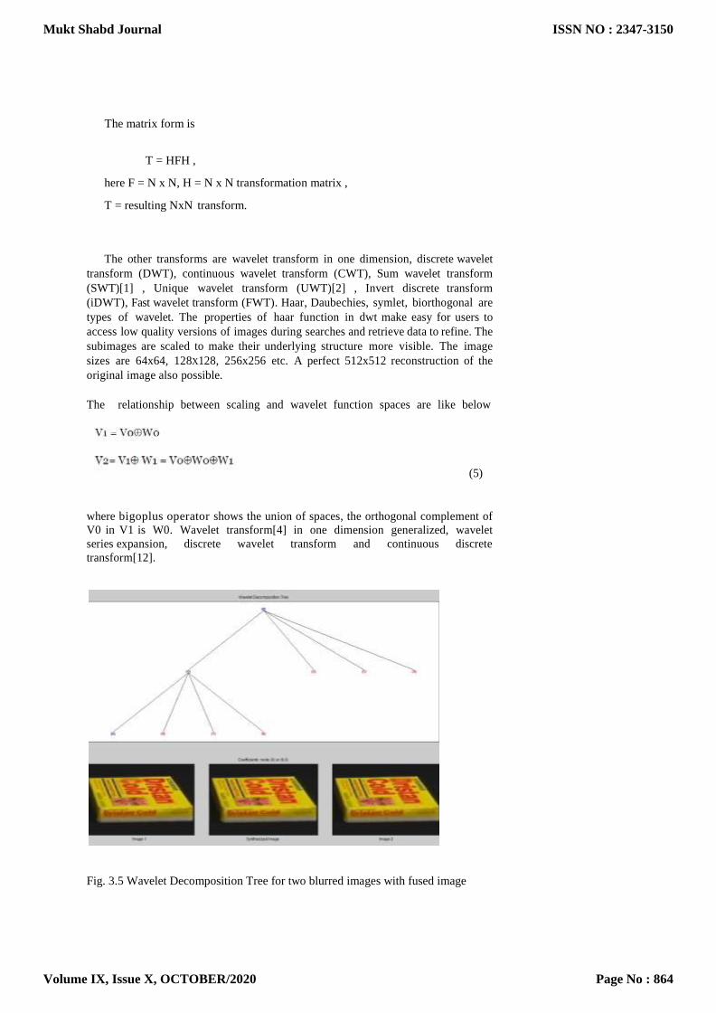
The matrix form is
T = HFH ,
here F = N x N, H = N x N transformation matrix ,
T = resulting NxN transform.
The other transforms are wavelet transform in one dimension, discrete wavelet
transform (DWT), continuous wavelet transform (CWT), Sum wavelet transform
(SWT)[1] , Unique wavelet transform (UWT)[2] , Invert discrete transform
(iDWT), Fast wavelet transform (FWT). Haar, Daubechies, symlet, biorthogonal are
types of wavelet. The properties of haar function in dwt make easy for users to
access low quality versions of images during searches and retrieve data to refine. The
subimages are scaled to make their underlying structure more visible. The image
sizes are 64x64, 128X128, 256x256 etc. A perfect 512x512 reconstruction of the
original image also possible.
The relationship between scaling and wavelet function spaces are like below
(5)
where bigoplus operator shows the union of spaces, the orthogonal complement of
V0 in V1 is W0. Wavelet transform[4] in one dimension generalized, wavelet
series expansion, discrete wavelet transform and continuous discrete
transform[12].
Fig. 3.5 Wavelet Decomposition Tree for two blurred images with fused image
Mukt Shabd Journal
Volume IX, Issue X, OCTOBER/2020
ISSN NO : 2347-3150
Page No : 864
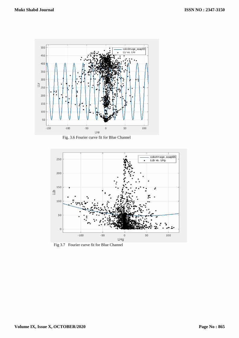
Fig. 3.6 Fourier curve fit for Blue Channel
Fig 3.7 Fourier curve fit for Blue Channel
Mukt Shabd Journal
Volume IX, Issue X, OCTOBER/2020
ISSN NO : 2347-3150
Page No : 865

Fig 3.8 Polynomial fit for Green channel graph of soap image 65
Fig 3.9 Gaussian Curve fitting between HLr and HLg
The above Fig 4.1 to 4.4 shows different curve fitting graph with coefficient
value 1. The dark dots are pixels. The dots plots on blue curve are fit enough. Thus
image fusion analysed with fourier, polynomial and Gaussian for LLr, LHr, LLb,
LHg, HLr and HLg.
Like the fourier series expansion[9], the wavelet series expansion maps a
function of continuous variable into sequence of wavelet coefficients. Hence the
resulting coefficients are called discrete wavelet transform (DWT) of f(x).
Mukt Shabd Journal
Volume IX, Issue X, OCTOBER/2020
ISSN NO : 2347-3150
Page No : 866

W j-1
D
W j-1
<----V--->(л)
W j-1
D
<---H ---- > W j-1
(-л)
V j-1
<---H--> W j-1
(л)
D
W j-1
<--- V ----- > (-л)
W j-1
D
W j-1
Fig.3.10 First decomposition of a 2 dimensional FWT spectrum
The natural extension of the discrete wavelet transform is the continuous wavelet
transform (CWT) by redundant function of two continuous variables translation
and scale. The fast wavelet transform (FWT) is an efficient dwt, good in
computation[8]. Inverse transform for the reconstruction of f(x) from DWT/FWT
approximation and coefficients can also be formulated. It is called as inverse fast
wavelet transform which uses the scaling and wavelet vectors employed in the
forward transform.
We can modify a DWT for edge detection also selected coefficients can
be deleted for better image reconstruction. We can replace the coefficients
by its subspace. The resultant is the image analysis tree. Analysis tree
supports unique decompositions. Analysis tree also an efficient mechanism for
representing wavelet packetS[12]. A wavelet packet tree supports 26 different
decompositions[11, 14].
VJ
V J-1 𝑤H - ……... 𝑤𝐷 𝐽−1 𝐽−1
Fig.3.7 Subspace analysis tree
In the above fig. 3.7 , as in the one dimensional case , generate P scale
transforms like j = J-1, J-2 ...J-P. In two dimensional nature of the input,
are denoted by wj−1H , wj−1
𝑉 , wj−1𝐷 wavelet subspaces, where H,V,D
are horizontal, vertical and diogonal directions.
Mukt Shabd Journal
Volume IX, Issue X, OCTOBER/2020
ISSN NO : 2347-3150
Page No : 867

4 Experimental Results and Performance Comparison
4.1 Fusion Factor (FF)
Fusion Factor is the combination of IFA and IFB factors. Where IFA is the
mutual information index between image ‘A’ and fused image, IFB is mutual
information index between image ‘B’ and fused image. Fusion Factor affects the
quality of an image. Higher value represents better data density.
FF = IFA + IFB (7)
4.2 Edge Strength (ES)
Edge Strength can be done using sobel edge operator. It calculates Gx, Gy for
image A and B,
G= √Gx2 + Gy2 (8) Higher edge strength more edge information.
4.3 Entropy
Entropy is the amount of information present in the image Here P is the
probability of pixel xi,
𝑁 𝑖=1 (𝑥𝑖) log2(𝑥𝑖) (9) E = - ∑
Mukt Shabd Journal
Volume IX, Issue X, OCTOBER/2020
ISSN NO : 2347-3150
Page No : 868
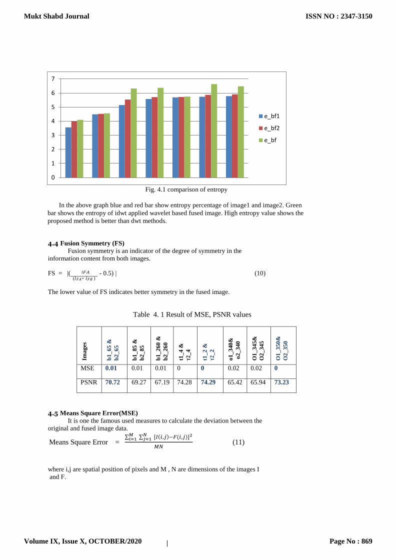
8
Fig. 4.1 comparison of entropy
In the above graph blue and red bar show entropy percentage of image1 and image2. Green
bar shows the entropy of idwt applied wavelet based fused image. High entropy value shows the
proposed method is better than dwt methods.
4.4 Fusion Symmetry (FS)
Fusion symmetry is an indicator of the degree of symmetry in the
information content from both images.
FS = |( 𝐼𝐹𝐴 - 0.5) | (10)
(𝐼𝐹𝐴+ 𝐼𝐹𝐵 )
The lower value of FS indicates better symmetry in the fused image.
Table 4. 1 Result of MSE, PSNR values
Ima
ges
b1_
65
&
b2
_6
5
b1_
85
&
b2
_8
5
b1_2
60
&
b2
_26
0
t1_4
&
T2_
4
t1_2 &
T2_
2
o1
_3
40
&
o2_
34
0
O1
_3
45&
O2
_34
5
O1
_3
50
&
O2
_35
0
MSE 0.01 0.01 0.01 0 0 0.02 0.02 0
PSNR 70.72 69.27 67.19 74.28 74.29 65.42 65.94 73.23
4.5 Means Square Error(MSE)
It is one the famous used measures to calculate the deviation between the
original and fused image data.
Means Square Error = ∑ ∑ [𝐼(𝑖,𝑗)−𝐹(𝑖,𝑗)]2𝑁
𝑗=1𝑀𝑖=1
𝑀𝑁 (11)
where i,j are spatial position of pixels and M , N are dimensions of the images I
and F.
0
1
2
3
4
5
6
7
e_bf1
e_bf2
e_bf
Mukt Shabd Journal
Volume IX, Issue X, OCTOBER/2020
ISSN NO : 2347-3150
Page No : 869

8
4.6 Peak Signal to Noise Ratio (PSNR)
The peak signal to noise ratio (PSNR) is the ratio of the maximum value of an
image and magnitude of background noises.
PSNR=10log10 (2𝑛−1)2
𝑀𝑆𝐸 (12)
4.7 Root Mean Square Error (RMSE)
This measurement is used to evaluate the fused image. Let be the fused
image, is the input image, then
Root Mean Square Error = √∑ ∑[𝐼(𝑖,𝑗)−𝐹(𝑖,𝑗)]2
𝑀𝑁 (13)
The results of MSE(Mean Square Error) gives very minimum value zero
for combination of t1_4 & t1_2, t1_2& t2_2 and O1_350 & O2_350
images. After fusion, again the size of images vary. So again resize the image using
preprocesss algorithm. The value of MSE and PSNR value for soap image is
0.09 and 58.51. The value of MSE and PSNR value for tomoto image is 0.01
and 69.48. The value of MSE and PSNR value for OralB image is 0.03 and 74.28.It
is notable that MSE value is increased in MSE value and decreased in PSNR
values, which are useful to identify the original and fused image in defence or
secured sectors.The restore of images can be done using fuzzy logic[10].
SSE is the sum of the squared difference between each observation and its
groups mean. It can be used as a measure of variation within a cluster. If all
cases within a cluster are identical then SSE would be equal to zero.
SSE = ∑𝑛 ( xi-Î)2 (14)
𝑖=1
where , n – number of observations xi –
is the value of the ith observation Î -is
mean of all observations
In cluster analysis , SSE
is minimized with
SSEtotal = SSE1+ SSE2+ SSE3.....+ SSEn (15)
Mukt Shabd Journal
Volume IX, Issue X, OCTOBER/2020
ISSN NO : 2347-3150
Page No : 870
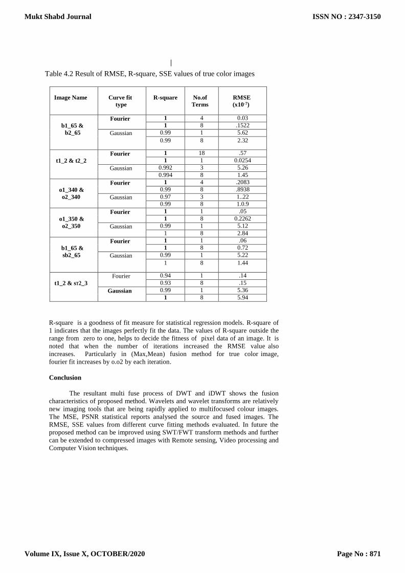
Table 4.2 Result of RMSE, R-square, SSE values of true color images
Image Name
Curve fit
type
R-square
No.of
Terms
RMSE
(x10-7)
b1_65 &
b2_65
Fourier 1 4 0.03
1 8 .1522
Gaussian 0.99 1 5.62
0.99 8 2.32
t1_2 & t2_2
Fourier 1 18 .57
1 1 0.0254
Gaussian 0.992 3 5.26
0.994 8 1.45
o1_340 &
o2_340
Fourier 1 4 .2083
0.99 8 .8938
Gaussian 0.97 3 1..22
0.99 8 1.0.9
o1_350 &
o2_350
Fourier 1 1 .05
1 8 0.2262
Gaussian 0.99 1 5.12
1 8 2.84
b1_65 &
sb2_65
Fourier 1 1 .06
1 8 0.72
Gaussian 0.99 1 5.22
1 8 1.44
t1_2 & sT2_3
Fourier 0.94 1 .14
0.93 8 .15
Gaussian 0.99 1 5.36
1 8 5.94
R-square is a goodness of fit measure for statistical regression models. R-square of
1 indicates that the images perfectly fit the data. The values of R-square outside the
range from zero to one, helps to decide the fitness of pixel data of an image. It is
noted that when the number of iterations increased the RMSE value also
increases. Particularly in (Max,Mean) fusion method for true color image,
fourier fit increases by o.o2 by each iteration.
Conclusion
The resultant multi fuse process of DWT and iDWT shows the fusion
characteristics of proposed method. Wavelets and wavelet transforms are relatively
new imaging tools that are being rapidly applied to multifocused colour images.
The MSE, PSNR statistical reports analysed the source and fused images. The
RMSE, SSE values from different curve fitting methods evaluated. In future the
proposed method can be improved using SWT/FWT transform methods and further
can be extended to compressed images with Remote sensing, Video processing and
Computer Vision techniques.
Mukt Shabd Journal
Volume IX, Issue X, OCTOBER/2020
ISSN NO : 2347-3150
Page No : 871
REFERENCES
1. Tapasmini Sahoo, Richa Acharya & kunal Kaumar Das,An Innovative approach of
multifocus Image Fusion using SWT and Content Adaptive Blurring, IJET, Vol
7,2018
2. A.Anoop Suraj, Mathew Fransis, Discrete Wavelet Transform based Image Fusion
and Denoising in FPGA ,JESIT,2014,72-81
3. Kumudham,Tarun,Avinash Rajendran, Resolution Enrichment using wavelet based
interpolation method
4. Amolins, K., Zhang, Y., Dare, P., 2007. Wavelet based image fusion techniques—
an introduction, review and comparison. ISPRS J. Photogram.Remote Sens. 62
(September (4)), 249–263.
5. Baradarani, A., Jonathan Wu, Q.M., Ahmadi, M., Mendapara, P., 2012. Tunable
halfband-pair wavelet filter banks and application to multifocusimage fusion.
Pattern Recogn. 45 (February (2)), 657–671.
6. VPS Naidu and J.R. Raol “Pixel-Level Image Fusion using Wavelets and Principal Component Analysis
A Comparative Analysis”, Defense Science Journal,Vol 58, No.3, pp.338-352, May 2008.
7. http://www.nasa.gov/centers/ames/research/2007/imagefusion.html
8. Irshad, H.; Kamran, M.; Siddiqui, A.B.; Hussain, A., Image fusion using
computational intelligence:A survey, Environmental and Computer Science, ICECS
’09. Second International Conference ,2009, pp.128- 132. 9. http://www.mathworks.fr/matlabcentral/fileexchange/28923-image-fusion
10. Jionghua Teng; Suhuan Wang; Jingzhou Zhang; Xue Wang, Neuro fuzzy logic
based fusion algorithm of medical images, Image and Signal Processing (CISP),
2010, 3rd International Congress, vol.4, pp.1552- 1556.
11. R. C. Gonzalea and R. E. Woods, Wavelets and Multiresolution Processing, Digital
Image Processing, 2004, 2nd Ed., Prentice Hal.
12. Ivan W. Selesnick, Richard G. Baraniuk, and Nick G. Kingsbury, The Dual-
Tree Complex Wavelet Transform, IEEE Signal Processing Magazine, 2005, vol.
22, no. 6, pp. 123-151.
13. Jingyu Yang, Yao Wang, Wenli Xu, and Qionghai Dai, Image Coding Using Dual-
Tree Discrete Wavelet Transform, IEEE Trans. Image Processing, 2008, vol. 17, no.
9, pp. 1555-1569.
14. Gonzalo Pajares, Jes us Manuel de la Cruz, A wavelet-based image fusion tutorial,
Pattern Recognition, 2004, pp.1855 1872.
Mukt Shabd Journal
Volume IX, Issue X, OCTOBER/2020
ISSN NO : 2347-3150
Page No : 872

See discussions, stats, and author profiles for this publication at: https://www.researchgate.net/publication/348575344
PREDICTION OF LIVER DISEASES USING DECISION TREES AND MACHINE
LEARNING ALGORITHMS
Article · January 2020
CITATIONS
0READS
132
1 author:
Some of the authors of this publication are also working on these related projects:
Data Classification View project
Pulmonary nodule identification View project
Piramu Kailasam
Sadakathullah Appa College
16 PUBLICATIONS 12 CITATIONS
SEE PROFILE
All content following this page was uploaded by Piramu Kailasam on 18 January 2021.
The user has requested enhancement of the downloaded file.

Journal of the Maharaja Sayajirao University of Baroda
ISSN : 0025-0422
Volume-54, No.2 (XIIX) 2020 157
PREDICTION OF LIVER DISEASES USING DECISION TREES AND MACHINE
LEARNING ALGORITHMS
S.Piramu Kailasam Assistant Lecturer, Sadakathullah Appa College,Tirunelveli
Abstract
Human body consists of various important organs for processing the entire metabolism of the human
being. Some of them are the kidneys, brain, heart and liver. The proper functioning of these organs
will lead the person happy life. The identification of problems to these organs is also important at the
right point of time. In the current article a GUI model had been developed such that to identify the
level of damage happened to liver based on the data given by users. The current model will also
provide the details about various problems that causes to the liver through GUI model. The saying in
the medical field is always predicting the disease in earlier stages is better than at the crucial period
such that to reduce the damage of that problem to that particular organ. The symptoms also become
more different and also difficult to analyze at later stages. In the current tool, an attempt had been
made to utilize the machine learning algorithms like K-means, ANN and SVM to analyze the liver
patients from a group of normal patients. The comparison of the machine learning algorithms for
their performance to identify the liver problems based on performance factors also observed. The
developed GUI can be a good source for the doctors to analyze liver diseases.
Keywords: Liver,Diseases,Machine learning, ANN, SVM, K-means
1. Introduction
Human body had a versatile number of parts which are playing a key role for the healthier life of any
human being. Some of those parts are brain, heart, liver, kidneys, etc,. The successful functioning of
these parts will lead the life any human being successful and a happy life [Dimitris Lipara et. Al.,
Kulwinder Kaur et. Al., Pooja Sharma et. Al.,]. The diseases or the problems occurring with these
parts may lead to great damage to the functioning of the human body. The major problem concerned
with these components was all these parts working metabolism depends on the functioning of other
parts of the body. The identification of problems with these parts and diagnosis at the right intervals
at right point of time is more important such that the further damage of the parts and the problem
spreading to other parts also can be reduced to some level. When the diseases to these organs are in
severe conditions, the symptoms are apparently changes from the regular types of symptoms and it
becomes difficult to identify when the diseases are in critical stages. With proper medication and
other measures taken by the patients, these problems can be reduced to some level of damage to the
other parts of the body. The currently developed application is a graphical user interfacing unit with
which the doctors or medical practitioners can utilize to identify the symptoms and give as input and
can identify the problems of liver diseases at various stages [Hao Jia, Manmohan Shukla et. Al.,
V.V.Ramalingam et. Al.,].
The current model is also used to identify the number of people with liver problems also identified
from the available list of patients. A group of patients and their blood samples and values are made
with databases and the data was given as input to the current model and list of patients with liver
problems are identified from the available list of total patients in the selected database.
About Liver
Liver is one of the important organs in the human body [G.Ignisha Rajitha et. Al., Esraa Mamdohi
Mai et. Al., Islam MM et. Al., Mei Ying et. Al.,]. The size of the liver is large and its place in the
human body is on the right side of the belly of the human being. The colour of the liver is red and
brown in colour. It always looks like the feel of a rubber type of material to touch. The tasks
performed by the liver in the human body are around 500 tasks [Abhijit singh Putu et. Al., MoonSun
Shin et. Al., Jung-euk Ahn et. Al.,]. The best feature of this organ is that it can regenerate at any
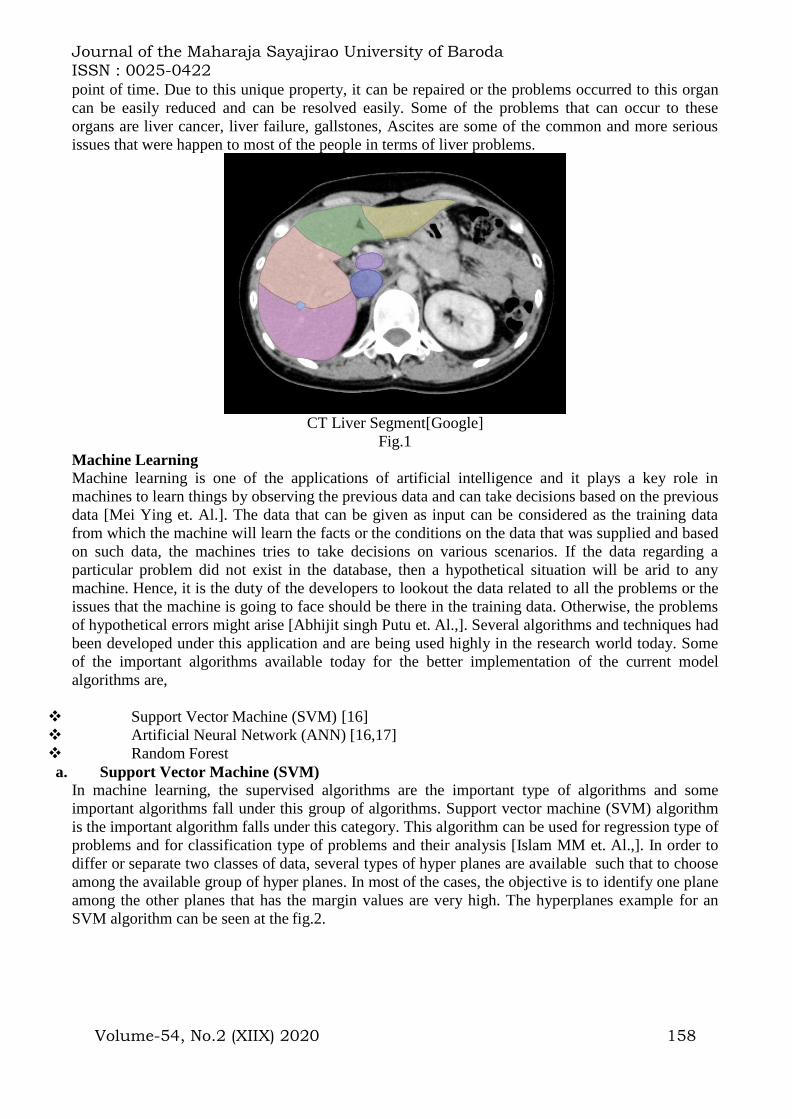
Journal of the Maharaja Sayajirao University of Baroda
ISSN : 0025-0422
Volume-54, No.2 (XIIX) 2020 158
point of time. Due to this unique property, it can be repaired or the problems occurred to this organ
can be easily reduced and can be resolved easily. Some of the problems that can occur to these
organs are liver cancer, liver failure, gallstones, Ascites are some of the common and more serious
issues that were happen to most of the people in terms of liver problems.
CT Liver Segment[Google]
Fig.1
Machine Learning
Machine learning is one of the applications of artificial intelligence and it plays a key role in
machines to learn things by observing the previous data and can take decisions based on the previous
data [Mei Ying et. Al.]. The data that can be given as input can be considered as the training data
from which the machine will learn the facts or the conditions on the data that was supplied and based
on such data, the machines tries to take decisions on various scenarios. If the data regarding a
particular problem did not exist in the database, then a hypothetical situation will be arid to any
machine. Hence, it is the duty of the developers to lookout the data related to all the problems or the
issues that the machine is going to face should be there in the training data. Otherwise, the problems
of hypothetical errors might arise [Abhijit singh Putu et. Al.,]. Several algorithms and techniques had
been developed under this application and are being used highly in the research world today. Some
of the important algorithms available today for the better implementation of the current model
algorithms are,
Support Vector Machine (SVM) [16]
Artificial Neural Network (ANN) [16,17]
Random Forest
a. Support Vector Machine (SVM)
In machine learning, the supervised algorithms are the important type of algorithms and some
important algorithms fall under this group of algorithms. Support vector machine (SVM) algorithm
is the important algorithm falls under this category. This algorithm can be used for regression type of
problems and for classification type of problems and their analysis [Islam MM et. Al.,]. In order to
differ or separate two classes of data, several types of hyper planes are available such that to choose
among the available group of hyper planes. In most of the cases, the objective is to identify one plane
among the other planes that has the margin values are very high. The hyperplanes example for an
SVM algorithm can be seen at the fig.2.

Journal of the Maharaja Sayajirao University of Baroda
ISSN : 0025-0422
Volume-54, No.2 (XIIX) 2020 159
Fig.2: Hyper planes example of an SVM Algorithm [Tom Bromley et. Al.,]
The value is high means it can be taken as that the distance between various points in those classes is
having the good margin. As this distance is more, the future classification is also done easily for
further future sources. These hyperplanes can also be considered as the boundary decisions to be
considered and also for identifying and classifying various pints of data in various databases. When
the program is being run, the data points will fall on both sides of the planes, both sides of the planes
data points can be considered as the data points belongs to two different classes of data.
b. Artificial Neural Networks
Neural networks are the one of the important applications of machine learning. The most important
thing in this model is the current model works on the mechanism of neurons in the human brain such
that to resemble the working of a neural systems in the human brain. The major applications or the
help that the users are getting from these networks are the cluster and classifying of data. Some of
the major applications of these neural network models are face detection, identifying the objects in
images, identifying the expression on faces, identifying the gestures in images and videos, detection
of voices, speech translation etc. The artificial neural network model can be seen clearly for better
understanding at fig.3.
Fig.3: Artificial Neural network model [Tom Bromley]
Some of the major applications of these neural network models are face detection, identifying the
objects in images, identifying the expression on faces, identifying the gestures in images and videos,
detection of voices, speech translation etc.
d. Random Forest
Classification is one of the major important considerations for any machine learning application.
Performing this classification task precisely will give us more accurate and better performances than
the expected ones. The major considerations are like predicting a customer for a product purchase or
predicting the mood of the customers to check whether the product will be purchased by the person
or not. All these sort of applications are key factors for the implementation of these random forest
algorithms. Basically this algorithm belongs to the family of decision trees which are used very
frequently for the identification of results from these sorts of applications. For better understanding

Journal of the Maharaja Sayajirao University of Baroda
ISSN : 0025-0422
Volume-54, No.2 (XIIX) 2020 160
of the random forest example, a model was presented at fig.4.
Fig.4: Random Forest Example [4]
In the working of the current algorithm, a various number of decision trees will present, these trees
are of two types built. At first, every single tree is built based on the data available or data getting
from the original database. And the next step is a subset of features are selected randomly from the
each near nodes and the new data set or the new result set of nodes which were classified are given as
output.
Roc Curve
ROC curve stands for the receiver operating the characteristic curve is basically used to represent the
data trends that were showing towards the true false and false true etc. Basically this plot is designed
by using the True positive rate and false positive rate at different threshold values.
Fig.5: An example of ROC curve model [5]
The mode of classification and the success rate of data classification can also be observed with this
curve as an output. Most of the researchers are using the same the mode of curve fro representing
various data classification techniques and models now days. In order to have the better
understanding of the ROC curve model, an example curve had been presented at fig.5.
2. Literature Review
Several authors had done various works on the area related to the current article. Some of the articles
and authors who had done some related works are discussed in the current section to identify the
similar set of works,
V.V. Ramalingam, A.Pandian, R. Ragavendran discussed about various algorithms that can be used
for identifying the problems of liver diseases in human beings. They had discussed in detail about
various algorithms of machine learning and decision trees, and also explained how these algorithms
can be used for further analysis of finding diseases in liver and its related components.
G. Ignisha Rajathi and G. Wiselin Jiji discussed in detail about the chronic diseases that might occur
with various symptoms and with several causes. All the symptoms and the disease issues were
discussed in detail with the help of various algorithms like the Simulated Annealing and Ensemble
Classifier. The results are very good and impressive and the identification of these serious diseases
can be found easily by utilizing this method of techniques further for achieving the better results.
Esraa MamdouhMai, Mabrouk Mai Mabrouk discussed about diabetes and chronic liver diseases and
the reasons for their presence in human bodies are also discussed in detail. SVM algorithm had given
some good resulted when their model was implemented with their own dataset.
Islam MM, Wu CC, Poly TN, Yang HC, Li YJ discussed about the fatty liver diseases and their
symptoms and the problems and solutions for the same diseases. They had used various machine
learning algorithms to identify the symptoms from the pool of items to be noted at various databases
and the algorithms for the same. The results and the utilization of the method are described in detail
and the results are interesting for further analysis and extensions of the works.
From the above works, almost all the works are done with the various machine learning algorithms.
Very few works are done with the combination of both machine learning and decision tree

Journal of the Maharaja Sayajirao University of Baroda
ISSN : 0025-0422
Volume-54, No.2 (XIIX) 2020 161
algorithms. Hence, in the current work an attempt has been made to analyze our new dataset with the
combination of both these types of algorithms and tried to analyze the performance of these
algorithms. The results and representations are discussed in detail in the form of ROC curve and
other values.
3. Proposed System
Several authors had considered several algorithms and methods to identify the presence of liver
related issues and diseases in human beings with the presence of various symptoms. If the detection
of these diseases were done at right intervals of time, the disease and its related issues can be
reduced to a great level of relief to these patients. In the current work, an attempt had been made to
analyze the performance of the two set of algorithms like the machine learning algorithms and the
decision trees algorithms. From the pool of the machine learning algorithms, we had considered the
SVM algorithm and the ANN algorithm and from the pool of decision trees algorithms Random
Forest algorithm had been chosen. The performance was analyzed by collecting the various set of
samples from various hospitals in Visakhapatnam and the results were displayed in the results
section.
4. Implementation and Results of the Current Methods
The implementation of the current model considered was done in the following process and the
detail process had explained as follows. For the better submission of data to analyze and to process,
an integrated graphical user interface had been developed such that to submit the data and to process
the data. The graphical interface had been developed with the PHP model and the algorithms which
were using in the current model are connected with the current GUI such that user can select the type
of algorithm he needs to implement or he can check the data with a particular algorithm. A drop
down menu had been created for the three set of algorithms and the user can select his choice of
algorithms and also the users can select all the three algorithms individually and can check the
results with three algorithms one after the other algorithm.
The disease symptoms and its values may vary sometimes to some levels in males and females.
Hence, it is always better to first classify the data for both male patients and female patients and then
apply the algorithm from the above selected three algorithms and try to get the results and conclude
with those set of results obtained from the above interfacing unit with each algorithm
implementation. The detailed architecture of the entire process had been presented in fig.6.
Fig.6: Architecture model of the current method and flow of execution
Whenever the data was being submitted by the user for checking with the currently developed
model, the machine will collect the knowledge or expertise from the database that we had already
submitted with previous results and symptoms. The machine learning algorithms needs to work on

Journal of the Maharaja Sayajirao University of Baroda
ISSN : 0025-0422
Volume-54, No.2 (XIIX) 2020 162
some existing data of patients such that to train from that particular data and take the decisions.
Hence, a set of patients data was collected from various hospitals and laboratories in and around the
Visakhapatnam City and a dataset of patients with both male and female with various ages had
prepared. Once the data is collected and dataset is prepared, the cleaning of the data and correlation
of the data is to be done and then the errors and noise in the database was removed for fast and easy
working of the machine with these algorithms. Once the entire process of this data analysis had
completed, the standard format of the data was prepared and the data needs to be analyzed for further
algorithms to get more accurate results based on the various symptoms and their values present.
Whenever the new choice of patient’s data is to be verified, the data is being verified and then the
current record of patient’s data was added to the existing dataset. Once the data is cleaned and ready
for checking the data had been distributed on the categorical basis. Then the data correlation and
cleaning of data had been completed and the algorithms are implemented and the data results are
represented in the form of ROC curve and the results presentation.
When the database is present with various patients’ data with various attributes, the dataset is
to be distributed with various numerical features. Some of those features are like age, albumin,
alamine_Aminotransfarese, Albumin and Globulin Ratio, Alkaline Phosphate, direct bilirubin, total
bilirubin, etc. The user interface of the current model was presented at fig.7 for better understanding.
Fig.7: The user interface of the current developed model
In order to understand the data and its components perfectly, exploratory data analysis and the
distribution of numerical features had been done such that for the better understanding of the trends
of the data. The exploratory data analysis model was presented in fig.8 and distribution of numerical
values is also observed in fig.9 in detail.
Fig.8: Exploratory Data Analysis
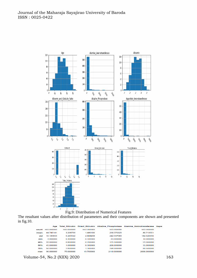
Journal of the Maharaja Sayajirao University of Baroda
ISSN : 0025-0422
Volume-54, No.2 (XIIX) 2020 163
Fig.9: Distribution of Numerical Features
The resultant values after distribution of parameters and their components are shown and presented
in fig.10.

Journal of the Maharaja Sayajirao University of Baroda
ISSN : 0025-0422
Volume-54, No.2 (XIIX) 2020 164
Fig.10: Resultant values after the proper distribution of values or the symptoms
Gender
Count 583
Unique 2
Top Male
Frequency 441
Fig.11: Distribution of categorical data
It seems there is outlier in Aspartate_Aminotransferase as the max value is very high than mean
value. Dataset i.e the output value has '1' for liver disease and '2' for no liver disease so let's make it 0
for no disease to make it convenient.
From the above table, the distribution of category and the features are plotted in the form of Bar
graph for better understanding of the values and the symptoms are presented in fig.11 and fig.12.
Fig.12: Bar plots for categorical Features
Number of patients that are male: 441
Number of patients that are female: 142
There are more male patients than female patients, Label Male as 0 and Female as 1. Once the data
labelling format is decided, the represented format of the data in the below dataset table I,
Table I. Dataset format with the representation of the labelling
The correlations between the various parameters and the symptoms and their values are represented
in the form of a table format with their represented values which are correlated with other. The
parameters considered with various symptoms and their values are represented at table II as,
Table II. Correlated values representation of symptom values
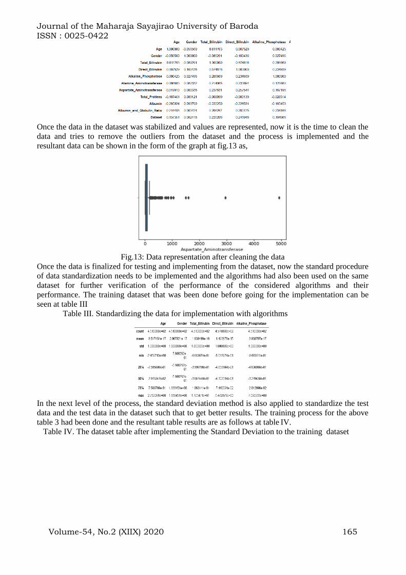
Journal of the Maharaja Sayajirao University of Baroda
ISSN : 0025-0422
Volume-54, No.2 (XIIX) 2020 165
Once the data in the dataset was stabilized and values are represented, now it is the time to clean the
data and tries to remove the outliers from the dataset and the process is implemented and the
resultant data can be shown in the form of the graph at fig.13 as,
Fig.13: Data representation after cleaning the data
Once the data is finalized for testing and implementing from the dataset, now the standard procedure
of data standardization needs to be implemented and the algorithms had also been used on the same
dataset for further verification of the performance of the considered algorithms and their
performance. The training dataset that was been done before going for the implementation can be
seen at table III
Table III. Standardizing the data for implementation with algorithms
In the next level of the process, the standard deviation method is also applied to standardize the test
data and the test data in the dataset such that to get better results. The training process for the above
table 3 had been done and the resultant table results are as follows at table IV.
Table IV. The dataset table after implementing the Standard Deviation to the training dataset

Journal of the Maharaja Sayajirao University of Baroda
ISSN : 0025-0422
Volume-54, No.2 (XIIX) 2020 166
At first, the Support Vector Machine is being implemented with the selected dataset and the results
are obtained in the form of both the ROC curve and actual values. The other two algorithms also had
followed the same type of process and the results obtained are shown and the final observation about
the performance of all the three algorithms are discussed and given the observations.
Case 1.
The results obtained for the SVM algorithm by calculating the ROC curve from the y_test and
predictions are observed at fig.14 as,
Fig.14: ROC curve for SVM algorithm
The accuracy of the above algorithm is observed as,
Case 2.
The results obtained for the Random Forest algorithm by calculating the ROC curve is presented at
fig.15 as,
Fig. 15: ROC curve for the second algorithm
The output result from the current algorithm as follows,

Journal of the Maharaja Sayajirao University of Baroda
ISSN : 0025-0422
Volume-54, No.2 (XIIX) 2020 167
5. Conclusions
In the current article, an attempt has been made to analyze and diagnose the liver diseases in patients
using various machine learning and decision trees algorithms. The machine learning and decision
trees algorithms are working perfectly on the selected and prepared dataset of various patients who
are suffering with various sliver diseases with various levels of the diseases. From the considered
three algorithms, the ANN model is having the better performance when compared to the other two
methods of algorithms. The GUI developed for performing the current applications and the tasks is
very useful and helpful for the normal people also to work on it. Any educated person also can work
on it with minimum knowledge of computer operations.
References [1] https://www.webmd.com/digestive- disorders/picture-of-the-liver#1 [Last Accessed on 10-03-2019]
[2] https://towardsdatascience.com/support-vector- machine-introduction-to-machine-learning- algorithms-
934a444fca47. [Last Accessed on 10- 03-2019]
[3] A blog written by Tom Bromley in Xanadu AI entitled, Making a Neural Network, Quantum” on February,
2018. [Last Accessed on 10-03-2019]
[4] Stavros I Dimitriadis, Dimitris Lipara (2018). How random is the random forest? Random forest algorithm on
the service of structural imaging biomarkers for Alzheimer's disease: from Alzheimer's disease neuroimaging
initiative (ADNI) database. Neural Regeneration Research, 13, 6, 962-970.
[5] A blog written by Jason Brownlee in Python Machine Learning in 2018 entitled “How and When to Use ROC
Curves and Precision-Recall Curves for Classification in Python”. [Last Accessed on 10-03-2019]
[6] Kulwinder Kaur and Vikas Zandu, (2016). A Secure Data Classification Model in Cloud Computing Using
Machine Learning Approach. International Journal of Grid and Distributed Computing, 9, 8, 13-22, SERSC
Australia.
[7] Pooja Sharma and A K Mishra (2017). Analysis and Classification of Plant microRNAs using Machine
Learning Approach. Asia-Pacific Journal of Neural Networks and Its Applications, 1, 2, 1-6, GVPress.
[8] Hao Jia (2015). Large-Scale Data Classification Method Based on Machine Learning Model. International
Journal of Database Theory and Application, 8, 2, 71-80, SERSC Australia.
[9] Manmohan Shukla, and B.K. Tripathi (2017). On the Efficient Machine Learning of the Fundamental Complex-
Valued Neurons. International Journal of Neural Systems Engineering, 1, 1, 21-26, GVPress.
[10] V.V. Ramalingam, A.Pandian, R. Ragavendran (2018). Machine Learning Techniques on Liver Disease - A
Survey. International Journal of Engineering & Technology, 7, 4.19, 485-495.
[11] G. Ignisha Rajathi, and G. Wiselin Jiji (2019). Chronic Liver Disease Classification Using Hybrid Whale
Optimization with Simulated Annealing and Ensemble Classifier. Symmetry, 11, 33, 1-21.
[12] Esraa MamdouhMai, MabroukMai Mabrouk, (2014). A Study of support vector machine algorithm for liver
disease diagnosis. American Journal of Intelligent Systems, 4, 1, 9-14.
[13] Islam MM, Wu CC, Poly TN, Yang HC, Li YJ (2018). Applications of Machine Learning in Fatty Live Disease
Prediction. Student Health Technological Information, 247, 166-170.
[14] Mei-ying Ren and Sin-jae Kang (2017). Korean 5W1H Extraction Using Rule-based and Machine Learning
Method. International Journal ofArtificial Intelligence and Applications for Smart Devices, 5, 2, 1-10, GVPress.
[15] Abhijitsingh Putu Gaonkar, Ritwik Kulkarni, Ronnie D. Caytiles and N.Ch.S.N Iyengar (2017). Classification
of Lower Back Pain Disorder Using Multiple Machine Learning Techniques and Identifying Degree of Importance
of Each Parameter. International Journal of Advanced Science and Technology, 105, 11-24, SERSC Australia.
[16] MoonSun Shin, HaYoung Lee, JinSoo Kim and JungHwan Kim (2018). Design of Intelligent Healthcare
Support System Applying Machine Learning. International Journal of Advanced Science and Technology, 111, 73-
84, SERSC Australia.
[17] Jung-euk Ahn, Eun-Surk Yi, Ji-Youn Kim and Byung Mun Lee (2018). A Multiracial Data-Based Machine
Learning Model for Exercise Motion Recognition. International Journal of Control and Automation, 11, 2, 89-102,
SERSC Australia.
View publication statsView publication stats

Prediction of Tuberculosis Diagnosis Using
Weighted KNN Classifier
S.Piramu Kailasam,
Assistant Professor, Department of Computer Applications,
Sadakathullah Appa College(Autonomous),
Tirunelveli,Tamil Nadu
Abstract
In this paper, a Machine learning Model is used to develop predictive model
for Tuberculosis diagnosis using classifiers. The Model is developed with Principle
Component Analysis for feature extraction and classified with Ensemble KNN
Classifiers. The data is transferred into the knowledge that the symptoms are the
significant ones in diagnosis Tuberculosis. The presented results showed that
Ensemble KNN classification accuracy for TB diagnosis is 91.4 % and training
time is 1.4661s, also analyzed with True positive rate and False positive rate.
Keywords: Tuberculosis, Principle Component Analysis, Machine learning
classifiers, Classification
1.Introduction
The Tuberculosis Chemotherapy Centre (as the NIRT was then known) was
set up in 1956 as a result of collaboration between ICMR (Indian Council of
Medical Research), BMRC (British Medical Research Council), USPHS (United
States Public Health Service), and the government of Tamil Nadu. It became the
Tuberculosis Research Centre (TRC) in the 1970s, and was renamed the National
Institute for Research in Tuberculosis (NIRT) recently. NIRT’s vision is to
undertake high quality research in Tuberculosis that is relevant to both national and
global programmatic needs.
The first research activity undertaken in 1956 (‘The Madras Study’) was
meant to compare the efficacy of drug treatment at home, for isolation in sanatoria
during the treatment duration for TB patients. The study found that cure rates were
the same in both settings, and there was no greater contact risk by leaving patients
at home. The results of this trial prompted OPD treatment of TB patients.
Mukt Shabd Journal
Volume X, Issue IV, APRIL/2021
ISSN NO : 2347-3150
Page No : 502

1.1 Tuberculosis
Tuberculosis[1,2] is an infectious disease caused by bacteria whose scientific
name is Mycobacterium tuberculosis. It was first isolated in 1882 by a German
physician named Robert Koch who received the Nobel Prize for this discovery. TB
most commonly affects the lungs but also can involve almost any organ of the
body. Tuberculosis (TB) is one of the most prevalent infections of human beings
and contributes considerably to illness and death around the world. It is estimated
by the World Health Organization (WHO) that one third of the global population is
infected with TB and that seven to eight million new cases of TB occur each year.
1.2 Cause of tuberculosis
Tuberculosis is not a hereditary disease. It is an infectious disease. Any
person can get afflicted with TB. Whenever, a patient having active tuberculosis
coughs or sneezes in an open manner, bacteria causing TB come out in the aerosol.
This aerosol can infect any person who happens to inhale it.
1.3 Symptoms of TB
Characteristic symptoms of TB are persistent cough of more than three
weeks duration, cough with expectoration of sputum, fever, weight loss or loss of
appetite etc. If any of these symptoms persist beyond three weeks, the person
concerned should visit the nearest DOTS TB Center or Health Center and get his
sputum examined.
1.4 Treatment of TB
If a full course of anti-tubercular drugs is taken on a regular basis, this
disease is fully curable. A TB patient has to take medicines for a minimum period
of six months continuously. The drugs may continue up to one year in some cases.
It is important that the drugs are discontinued only on the advice of the doctor.
Patients who do not take a complete treatment or take drugs on an irregular basis,
their disease turns incurable or even life-threatening.
1.5 Prevention
TB is a preventable disease, even in those who have been exposed to an
infected person. Skin testing (PPD) for TB is used in high risk populations or in
people who may have been exposed to TB, such as health care workers. A positive
skin test indicates TB exposure and an inactive infection. Discuss preventive
therapy[3] with your doctor. People who have been exposed to TB should be skin
tested immediately and have a follow-up test at a later date, if the first test is
Mukt Shabd Journal
Volume X, Issue IV, APRIL/2021
ISSN NO : 2347-3150
Page No : 503

negative. Prompt treatment is extremely important in controlling the spread of TB
from those who have active TB disease[3] to those who have never been infected
with TB[4,5].
2.Material and Methodology
Fig. 1 System Architecture
TB input dataset is taken as .csv file. Feature Extraction process is taken over
by PCA approach. Classified by SVM,Decisin tree, and KNN ensemble classfiers.
For the purpose of the study and analysis the data was taken from the records
of National Institute For Research In Tuberculosis
Number of Records : 430
Number of features : cough, fever, Hameoptisis, chestpain, weightloss,
dyspnoea, smear
The incidence of Tuberculosis is considered as the output feature while all the
other six features are taken as input features. The value attached on the title of each
column represents the maximum point that a patient can score on such symptoms.
As a patient is examined for any of the symptoms a score that represents the
medical practitioner in respect of the system is recorded for the patient. Based on
all the recorded values, the patient is diagnosed. Data set is divided into two sets
randomly as Training 70% , Testing Data 30% . In this work, Matlab 2016, intel
core i3 labtop, 6GB RAM is used.
TB Dataset
TB Disease
Diagnosis
Predictor Result
TB Disease
Diagnosis
Final Result
Classification using SVM, Decision
Tree, Logistic Regression and
Ensemble
KNN Classifiers
(ROC METHOD)
Feature
Extraction
using PCA
algorithm
Mukt Shabd Journal
Volume X, Issue IV, APRIL/2021
ISSN NO : 2347-3150
Page No : 504

2.2 Artifical neural networks
Artifical neural network consists of many nodes processing units analogous
to neuron in the brain. Each node has a node function associated with it which
along with a set of local parameter determines the output of the nodes, given an
input modifying the local parameters alter the node function. Artifical neural
network is an information processing system. In this information processing
system, the elements called neurons, process the information. The signals are
transmitted by means of connection links. The links possess an associated weight,
which is multiplied along with the incoming signal for any typical neural net. The
output signal is obtained by applying activations to the net input.
The neural net can generally be single layer or a multilayer net. Thus
artificial neural network represents the major extension to computation. They
perform the operations similar to that of the human brain. Hence it is reasonable to
except a rapid increase in our understanding of artifical neural network leading to
improved neural network paradigms and a host of application opportunies.
A simple artifical neural net with two input neurons ( ) and one output
neuron(y).The interconnected weights are given by and .In a single layer net
there is a single layer of weighted interconnections.
2.3 Machine learning
Supervised machine learning method is used to classify tb data. Feature
extraction and dimension reduction combined using Principle Component
Analysis technique. K nearest neighbor classifier finds K neighbours which are
similar like points and for distance it can uses Euclidean or cosine similarity. KNN
is suitable for low dimension space. In high dimension space like video frame
classification KNN is not suitable. In KNN classification model[6], Euclidian
distance metric and k value can alter depends upon data.
Ensemble KNN classifier used in this work are as follows. Fine KNN
classifier that classifies the data with neighbor value 1. Medium classifier that
classifies with number of neighbours as 10. Coarse KNN classifier[6] which makes
the classification between classes with number of neighbours value as 100. Cosine
classifier[6] that uses cosine distance metric. Cubic KNN classifier uses the cubic
distance metric. Weighted KNN classifier[6] which uses distance weighting. In
KNN classifier Euclidian distance is measured other than cubic classifier. In cubic
KNN classifier , Minkowski distance used.
Mukt Shabd Journal
Volume X, Issue IV, APRIL/2021
ISSN NO : 2347-3150
Page No : 505

3.Results and Discussion
ROC Curve Graph
Logistic Regression 89.4% SVM 88.5%
KNN Medium 89.1% Coarse KNN 72%
Fig 2. Accuracy of Classification models
ROC Curve
Cosine KNN 88.2% Cubic KNN 89.2%
Mukt Shabd Journal
Volume X, Issue IV, APRIL/2021
ISSN NO : 2347-3150
Page No : 506

Fine KNN 84.1% Weighted KNN 91.4%
Simple Decision Tree 87.9%
Fig. 3 Accuracy of Classification models
Mukt Shabd Journal
Volume X, Issue IV, APRIL/2021
ISSN NO : 2347-3150
Page No : 507
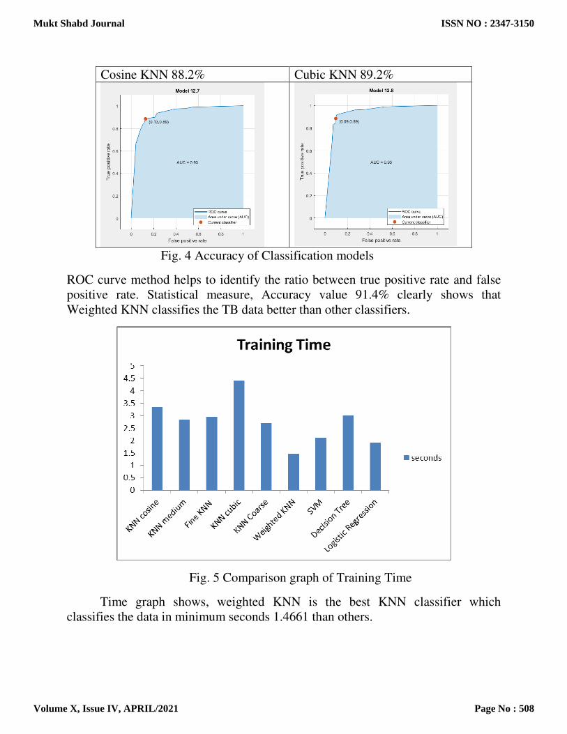
Cosine KNN 88.2% Cubic KNN 89.2%
Fig. 4 Accuracy of Classification models
ROC curve method helps to identify the ratio between true positive rate and false
positive rate. Statistical measure, Accuracy value 91.4% clearly shows that
Weighted KNN classifies the TB data better than other classifiers.
Fig. 5 Comparison graph of Training Time
Time graph shows, weighted KNN is the best KNN classifier which
classifies the data in minimum seconds 1.4661 than others.
Mukt Shabd Journal
Volume X, Issue IV, APRIL/2021
ISSN NO : 2347-3150
Page No : 508

4.Conclusion
Using recent improved machine learning algorithm to establish a
classification model for the diagnosis of TB with weighted KNN classifier shows
the better diagnostic performance. In this aspect, accuracy of weighted KNN
classifier is superior to ANN, logistic regression, SVM and decision tree
classifiers. The training time also better than other classifiers with PCA feature
extraction. In future, this work can extend with Artificial Intelligence technique.
References
1.Ren, Z., Hu, Y. & Xu, L. Identifying tuberculous pleural effusion using artificial intelligence
machine learning algorithms. Respir Res 20, 220 (2019).
2.Ryan H, Yoo J, Darsini P. Corticosteroids for tuberculous pleurisy. Cochrane Database Syst
Rev. 2017;3:CD001876.
3.Porcel JM. Biomarkers in the diagnosis of pleural diseases: a 2018 update. Ther Adv Respir
Dis. 2018;12:1753466618808660d.
4.Choi H, Chon HR, Kim K, et al. Clinical and laboratory differences between lymphocyte- and
neutrophil-predominant pleural tuberculosis. PLoS One. 2016;11(10):e0165428.
5.Li D, Shen Y, Fu X, et al. Combined detections of interleukin-33 and adenosine deaminase for
diagnosis of tuberculous pleural effusion. Int J Clin Exp Pathol. 2015;8(1):888–93.
6.Sameh Alfere, Ashraf Yunis maghari, Prediction of student’s performance using modified
KNN classifers. Ist international conference on Engineering and future technology, 2018.
Mukt Shabd Journal
Volume X, Issue IV, APRIL/2021
ISSN NO : 2347-3150
Page No : 509

S.Lingeswari et al, International Journal of Computer Science and Mobile Computing, Vol.10 Issue.8, August- 2021, pg. 51-59
© 2021, IJCSMC All Rights Reserved 51
Available Online at www.ijcsmc.com
International Journal of Computer Science and Mobile Computing
A Monthly Journal of Computer Science and Information Technology
ISSN 2320–088X IMPACT FACTOR: 7.056
IJCSMC, Vol. 10, Issue. 8, August 2021, pg.51 – 59
A STUDY OF TOMATO FRUIT DISEASE
DETECTION USING RGB COLOR
THRESHOLDING AND K-MEANS CLUSTERING
S.Lingeswari1; Dr. P.M.Gomathi
2; S.Piramu Kailasam
3
1Assistant Professor, P.K.R. Arts College for Women, Gobichettipalayam 2Head & Associate Professor, P.K.R. Arts College for Women, Gobichettipalayam
3Assistant Professor, Sadakathullah Appa College, Tirunelveli 1 [email protected];
2 [email protected]; 3 [email protected]
DOI: 10.47760/ijcsmc.2021.v10i08.009
Abstract— The agriculture field plays vital role in development of smart India. To increase economic level the production
of fruits, crops and vegetables can use CAD technique using image processing tools. Identifying diseases in fruits is an
image processing’s big challenging task. This can done by continuous visual photos or videos monitoring system. The
automated image processing research helps to control the pesticides on fruits and vegetables. In this paper we focus to
detect the diseases of tomato at earlier stage. The proposed system shows how different algorithms such as color
thresholding segmentation techniques and K-means clustering are used. In proposed system shows the K-means Clustering
is better than RGB color based colorthresholder method for detecting tomato diseases in beginning stage.
Keywords— Tomato disease, Threshold, Colorthresholding segmentation, K-means Clustering segmentation
I. INTRODUCTION
Image Segmentation[1] is an important part for processing the segment of an image into many disjoint small area based on
the certain principle, and it is one of the most basic area of research in the image processing. Image segmentation[1] is used in
many applications such as film and photo analysis, geo information systems, medical image analysis, satellite image analysis
and etc. Image segmentation of tomato images is the most important stage in detecting diseases. This stage carries to next process namely classification which classifies the tomato images in detail. There are many more segmentation methods and
algorithms available in object detection.
II. RELATED WORKS
Qimei Wang, MingheSun, JianhuaQu and JieXue authors Identify tomato diseases[2,14] and Detect the infected areas using CNN and Object Detection Techniques. Experimental result Indicate that ResNet -101 has the highest detection rate but
take longest time for training and detection.
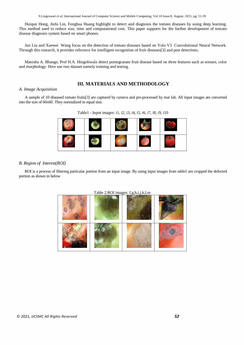
S.Lingeswari et al, International Journal of Computer Science and Mobile Computing, Vol.10 Issue.8, August- 2021, pg. 51-59
© 2021, IJCSMC All Rights Reserved 52
Huiqun Hong, Jinfa Lin, Fenghua Huang highlight to detect and diagnosis the tomato diseases by using deep learning. This method used to reduce size, time and computational cost. This paper supports for the further development of tomato
disease diagnosis system based on smart phones.
Jun Liu and Xuewei Wang focus on the detection of tomato diseases based on Yolo V3 Convolutional Neural Network.
Through this research, it provides reference for intelligent recognition of fruit diseases[3] and pest detections.
Manisha A. Bhange, Prof H.A. Hingoliwala detect pomegranate fruit disease based on three features such as texture, color and morphology. Here use two dataset namely training and testing.
III. MATERIALS AND METHODOLOGY A. Image Acquisition
A sample of 10 diseased tomato fruits[3] are captured by camera and pre-processed by mat lab. All input images are converted
into the size of 60x60. They normalized in equal size.
Table1 - Input images: i1, i2, i3, i4, i5, i6, i7, i8, i9, i10
B. Region of Interest(ROI)
ROI is a process of filtering particular portion from an input image. By using input images from table1 are cropped the defected
portion as shown in below
Table 2.ROI images: f,g,h,i,j,k,l,m

S.Lingeswari et al, International Journal of Computer Science and Mobile Computing, Vol.10 Issue.8, August- 2021, pg. 51-59
© 2021, IJCSMC All Rights Reserved 53
Fig 1.Work Flow Diagram
C. Pre-processing
Filtering[11] act as an important technique for modifying or enhancing the quality of an image. Filtering gives smoothing, sharpening and clear edges of an image. Image processing supports different types of filtering such as Gaussian filter, Bilateral filter,
Linear filter, Sigma filter[16 ], Median filter[11], etc. In this study, apply median filter for removing noise from an image. It is a non-
linear based filtering. In median filter, the center pixel of an MxN neighbourhood is replaced by the median (middle) value of the
corresponding window. It can be calculated by sorting all the pixel values from the matrix into numerical order and replace the pixel
value by using the median (middle) pixel value. In this paper apply 3x3 sampling window for filtering an images.
IV. TECHNIQUES USED IN SEGMENTATION PROCESS
Segmentation
Techniques
Advantages Disadvantages
Threshold[9,16]
It is a simple method and involves comparing each
pixel values of an image. It is applicable for only gray scale images.
It is not suitable
for blurred, outlier and noisy
images
ColorThresholder It is an advanced method of Threshold[9]. It used
colorimage[10] for comparing each pixel values for
segmentation.
It is not suitable
for edge based
computation.
K-means
Clustering[12]
(k=3)
It is more easy way to segment an image. Also it used
to eliminate noisy spots in an image
More expensive
for computation.
Image Acquisition
Preprocessing
(Median Filtering)
ColorThresholder
method
(RGB)
K means Clustering
method
(k = 3)
Detection of Tomato
Disease
Image Segmentation

S.Lingeswari et al, International Journal of Computer Science and Mobile Computing, Vol.10 Issue.8, August- 2021, pg. 51-59
© 2021, IJCSMC All Rights Reserved 54
V. RESULTS AND DISCUSSION A. Image Segmentation
ColorThresholding Method
To reduce noise, Median filter method[11] is applied to images. The Colorthresholder enables to create a segmentation
mask of a tomato[6] color image based on the exploration of different color spaces like RGB[15], HSV and La*b. As the fig.
shows segmented area of tomato. Threshold[5] only works with grayscale images. The image type is 8 bit. It is converted to
RGB stack. Color image is split into channels. Then adjusted Color Threshold values which are from 0 to 255.
Segmentation[1] achieved when Red, green, blue channels are adjusted. Green channel values are dominated than red and
blue. Secondly red takes good role in display segmented area. Blue channel has very least role in colorthresholding
segmentation.
Segmentation using colorthresholder algorithm
Input: Color images
Output: Detect the infected areas in the tomato
Step1: Read color images
Step2: Apply red color range between 0 and 255, then find threshold value. If threshold value reached then go to step5
Step3: Apply green color range between 0 and 255, then find threshold value. If threshold value reached then go to step5
Step4: Apply blue color range between 0 and 255, then find threshold value. If threshold value reached then go to step5
Step5: Stop the process
Step6: Finally compared the threshold values of each color and find which color is best for finding the infected area of an image.
Table 3.Colorthresholder Images and its color spaces
Input image Color space Output image

S.Lingeswari et al, International Journal of Computer Science and Mobile Computing, Vol.10 Issue.8, August- 2021, pg. 51-59
© 2021, IJCSMC All Rights Reserved 55
Table4: Qualitative analysis of segmented area (ColorThresholding method)
Images Mean Standard deviation
f 58.7 48.49
g 53.9 50.52
h 56.73 42.30
i 124.95 84.97
j 80.57 70.41
k 31.64 21.05
l 147.61 107.59
m 106.47 68.83
K-means Clustering
Data Mining is a process of extracting information from raw data. Data mining is an inter-process knowledge which includes
statistics, image processing, data base, machine learning and artificial intelligence. The different data mining techniques are
classification, clustering and regression, sequential pattern recognition and outlier detection. Clustering belongs to unsupervised
learning. A cluster is a subset of similar objects. Some of the clustering algorithms are Kmeans, hierarchical, fuzzy c means[17] and
DBSCAN algorithm. Kmeans clustering method is used for conducting image segmentation and disease detection. In this study Kmeans clustering algorithm is used for grouping related pixels which helps to detect the disease in tomato fruit image.

S.Lingeswari et al, International Journal of Computer Science and Mobile Computing, Vol.10 Issue.8, August- 2021, pg. 51-59
© 2021, IJCSMC All Rights Reserved 56
Segmentation Using K-means Clustering Algorithm
Step1: Read Image
Step2: Convert image from RGB color space to La*b* color space
Step3: Classify the colors in “a*b*” space using kmeans clustering
Step4: Label every pixel in the image using the results from kmeans
Step5: Create images that segment the tomato image by color
Table 5.Segmented images using Kmeans Clustering technique
Input image Cluster1 Cluster2 Cluster3
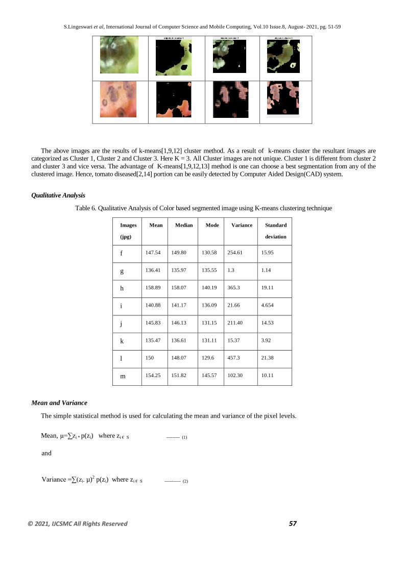
S.Lingeswari et al, International Journal of Computer Science and Mobile Computing, Vol.10 Issue.8, August- 2021, pg. 51-59
© 2021, IJCSMC All Rights Reserved 57
The above images are the results of k-means[1,9,12] cluster method. As a result of k-means cluster the resultant images are categorized as Cluster 1, Cluster 2 and Cluster 3. Here K = 3. All Cluster images are not unique. Cluster 1 is different from cluster 2
and cluster 3 and vice versa. The advantage of K-means[1,9,12,13] method is one can choose a best segmentation from any of the
clustered image. Hence, tomato diseased[2,14] portion can be easily detected by Computer Aided Design(CAD) system.
Qualitative Analysis
Table 6. Qualitative Analysis of Color based segmented image using K-means clustering technique
Images
(jpg)
Mean Median Mode Variance Standard
deviation
f 147.54 149.80 130.58 254.61 15.95
g 136.41 135.97 135.55 1.3 1.14
h 158.89 158.07 140.19 365.3 19.11
i 140.88 141.17 136.09 21.66 4.654
j 145.83 146.13 131.15 211.40 14.53
k 135.47 136.61 131.11 15.37 3.92
l 150 148.07 129.6 457.3 21.38
m 154.25 151.82 145.57 102.30 10.11
Mean and Variance
The simple statistical method is used for calculating the mean and variance of the pixel levels.
Mean, µ=∑zi * p(zi) where zi € S --------- (1)
and
Variance =∑(zi- µ)2 p(zi) where zi € S ----------- (2)
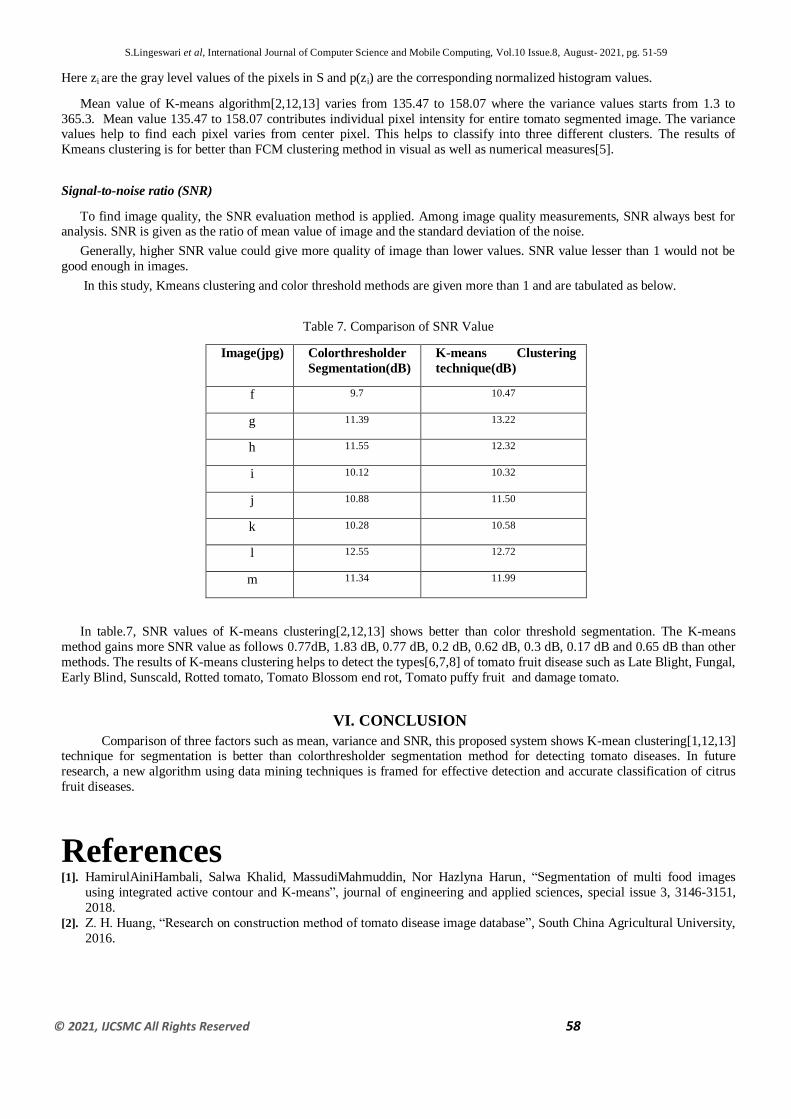
S.Lingeswari et al, International Journal of Computer Science and Mobile Computing, Vol.10 Issue.8, August- 2021, pg. 51-59
© 2021, IJCSMC All Rights Reserved 58
Here zi are the gray level values of the pixels in S and p(zi) are the corresponding normalized histogram values.
Mean value of K-means algorithm[2,12,13] varies from 135.47 to 158.07 where the variance values starts from 1.3 to
365.3. Mean value 135.47 to 158.07 contributes individual pixel intensity for entire tomato segmented image. The variance values help to find each pixel varies from center pixel. This helps to classify into three different clusters. The results of
Kmeans clustering is for better than FCM clustering method in visual as well as numerical measures[5].
Signal-to-noise ratio (SNR)
To find image quality, the SNR evaluation method is applied. Among image quality measurements, SNR always best for analysis. SNR is given as the ratio of mean value of image and the standard deviation of the noise.
Generally, higher SNR value could give more quality of image than lower values. SNR value lesser than 1 would not be
good enough in images.
In this study, Kmeans clustering and color threshold methods are given more than 1 and are tabulated as below.
Table 7. Comparison of SNR Value
Image(jpg) Colorthresholder
Segmentation(dB)
K-means Clustering
technique(dB)
f 9.7 10.47
g 11.39 13.22
h 11.55 12.32
i 10.12 10.32
j 10.88 11.50
k 10.28 10.58
l 12.55 12.72
m 11.34 11.99
In table.7, SNR values of K-means clustering[2,12,13] shows better than color threshold segmentation. The K-means
method gains more SNR value as follows 0.77dB, 1.83 dB, 0.77 dB, 0.2 dB, 0.62 dB, 0.3 dB, 0.17 dB and 0.65 dB than other
methods. The results of K-means clustering helps to detect the types[6,7,8] of tomato fruit disease such as Late Blight, Fungal,
Early Blind, Sunscald, Rotted tomato, Tomato Blossom end rot, Tomato puffy fruit and damage tomato.
VI. CONCLUSION
Comparison of three factors such as mean, variance and SNR, this proposed system shows K-mean clustering[1,12,13] technique for segmentation is better than colorthresholder segmentation method for detecting tomato diseases. In future
research, a new algorithm using data mining techniques is framed for effective detection and accurate classification of citrus
fruit diseases.
References [1]. HamirulAiniHambali, Salwa Khalid, MassudiMahmuddin, Nor Hazlyna Harun, “Segmentation of multi food images
using integrated active contour and K-means”, journal of engineering and applied sciences, special issue 3, 3146-3151,
2018.
[2]. Z. H. Huang, “Research on construction method of tomato disease image database”, South China Agricultural University,
2016.

S.Lingeswari et al, International Journal of Computer Science and Mobile Computing, Vol.10 Issue.8, August- 2021, pg. 51-59
© 2021, IJCSMC All Rights Reserved 59
[3]. Jagdeesh D. Pujari, Rajesh Yakkundimath, Abdulmunaf S. Byadgi, ”Statistical Methods for Quantitatively Detecting
Fungal Disease from Fruit’s Image”, International Journal of Intelligent System and Application in
Engineering,vol.1(4),60-67,2013.
[4]. ManishaBhange, H.A.Hingoliwala, “Review of Image Processing for Pomegranate Disease Detection”, International
Journal of Computer Science and Information Technologies, vol.6(1), 92-94,2015. J. Comp. Tech. Appl., Vol 2(5), 1709-
1716, 2011. [5]. M.MohamedSathik, S.PiramuKailasam, “Pulmonary CT image analysis for nodule detection using inspired FCM
clustering”, International Journal of Engineering Research & Technology (IJERT), vol.8(7),1013-1020, 2019.
[6]. ManyaAfonso, Hubert fonteijn, Felipe schadeck fiorentin, Dick Lensink, “Tomato fruit detection and counting in
greenhouse using deep learning”, Frontiers Plant Science, Vol. 11,1- 11, 2020.
[7]. Jiayue Zhao, JianhuaQu, “A detection method for tomato fruit common physiological diseases based on Yolov2”,
International Conference on Information Technology in Medicine and Education(ITME), 559-563, 2019.
[8]. Qimei Wang, Feng Qi, Minghe Sun , JianhuaQu, JieXue, “Identification of Tomato Disease Types and Detection of
Infected Areas Based on Deep Convolutional Neural Networks and Object Detection Techniques”, Computational
Intelligence and Neuroscience Volume 2019, 1-15.
[9]. SwapanSamaddar, Dr. A RamaSwamy Reddy, “Comparative study of image segmentation techniques on chronic kidney
diseases”, International Journal of Pure and Applied Mathematics, Volume 118,235-239, 2018.
[10]. TejasDeshpande, SharmilaSengupta, K.S. Raghuvanshi, “Grading Identification of Disease in Pomegranate Leaf and Fruit”, International Journal of Computer Science and Information Technologies, vol.5(3), 4638- 4645, 2014.
[11]. R. Gonzalez, R. Woods, Digital Image Processing, 3rd ed., Prentice- Hall, 2007.
[12]. Pham, V.H., Lee, B.R. “An image segmentation approach for fruit defect detection using k-means clustering and graph-
based algorithm”, Vietnam J ComputSci 2, 25–33, 2015.
[13]. Md. TarekHabib , AnupMajumder , A.Z.M. Jakaria , MoriumAkter, Mohammad ShorifUddin , Farruk Ahmed, “Machine
vision based papaya disease recognition “, Journal of King Saud University – Computer and Information Sciences,300-
309, 2020.
[14]. H. Hong, J. Lin and F. Huang, "Tomato Disease Detection and Classification by Deep Learning," 2020 International
Conference on Big Data, Artificial Intelligence and Internet of Things Engineering (ICBAIE), 2020, pp. 25-29, doi:
10.1109/ICBAIE49996.2020.00012.
[15]. HoreaMuresan, MihaiOltean, “Fruit recognition from images using deep learning”, act auniv.Sapientiae, informatica, 10, 1,26–42,2018.
[16]. SPKailasam, MMSathik,” A Reliable Computer Aided Lung Cancer Classification System Using Curvelet Features and
Ensemble Classifier”, International Journal of Pure and Applied Mathematics 117 (22), 275-278, 2017.
[17]. Ali,I.,Ahmed, A, “Segmentation of different fruits using image processing based on fuzzy C-means method”, 7th
international conference on reliability, ICRITO, pp-441-447, IEEE, 2018.

Journal of Analysis and Computation (JAC) (An International Peer Reviewed Journal), www.ijaconline.com, ISSN 0973-2861
Volume XIII, Issue I, January 2019
S. Mohideen Pillai and Dr. S. Kother Mohideen 1
FOOD IMAGE PROCESSING TECHNIQUES: A SURVEY
S. Mohideen Pillai1, Dr. S. Kother Mohideen2
1Reg.No : 18221252161009, Research Scholar, Department of IT, Sri Ram Nallamani Yadava College
of Arts & Science, Tenkasi, Tamilnadu – 627804, India, Affiliation of Manonmaniam Sundaranar
University, Abishekapatti, Tirunelveli – 627012, Tamilnadu, India. 2Associate Professor & Head, Department of IT, Sri Ram Nallamani Yadava College of Arts & Science,
Tenkasi, Tamilnadu – 627804, India.
ABSTRACT
As people across the globe are becoming more interested in watching their weight, eating more healthy and
avoiding obesity, a system that can measure calories and nutrition in every day meals can be very useful.
To identify food items accurately in such systems, image processing is used. Image processing techniques
like image segmentation, feature extraction, object recognition, classification is used for food recognition,
nutrients identification and calorie calculation. Bag-of-Features model, Artificial Neural Networks is used
to identify the food items. Image classifiers are trained to identify and categorize individual food items in
single image. This survey addressed various food image processing techniques, evaluates them and
presents the issues related to those techniques.
Keywords: Food recognition, Segmentation, Classification
[1] INTRODUCTION
One of the major goal of food image processing is to retrieve calorie and nutrient information
from the given food image. Food recognition is worthy of more research effort owning to its practical
signification and scientific challenges. Food recognition exposes new challenges to the current pattern
recognition literature and stimulates the stemming of novel techniques for general object recognition. In
addition, automatic food recognition is beneficial to health care related applications, such as obesity
management.
Obesity has become a serious public health problem to general population in many developed
countries [1], [2].The WHO defines obesity based on the Body Mass Index (BMI) of the individual. A
person is considered obese when the BMI is greater than or equal to 30(kg/m2) [2].Thus it is noticeable
that obesity and overweight are linked to a number of chronic diseases such as type II diabetes, breast
and colon cancer and heart diseases. The main cause of obesity is the imbalance between the amount of
food intake and energy consumed by the individuals [3].Obesity treatment requires the patient to

FOOD IMAGE PROCESSING TECHNIQUES: A SURVEY
S. Mohideen Pillai and Dr. S. Kother Mohideen 2
consume healthy food and decrease the amount of daily food intake, but in most of obesity cases it is
not easy for the patients to measure or control their daily intake due to the lack of nutrition education or
self-control. Therefore using an assistive monitoring food system is very needed and effective for
obesity elimination. Our objective is to develop an efficient food processing system to calculate the
calorie and nutrition of food. In this paper, general architecture, survey and analysis of various food
processing techniques are proposed.
The rest of the paper is organized as follows. Section 2 describes the various existing food
processing techniques. Section 3 covers the analysis of classifier used in the food processing
techniques. Finally, Section 4 concludes this paper with proposed work.
General Architecture of Food Processing System
Fig. 1 General Architecture
The general architecture of a Food Processing system is shown in Fig. 1. At the early stage, the quality
of the input food image is improved by image preprocessing techniques. In preprocessing: removing
noise, normalizing image, image format conversion, image resizing and removing unnecessary features
are carried out in the given image to improve the quality. In segmentation step, the image will be
analyzed to extract various segments of the food portion. For the detected food portions, a feature
extraction process has to be performed. In this step, various food features including size, shape, color,
and texture will be extracted. The extracted features will be sent to classifier, where the food portion
will be identified. Finally, by estimating the area and volume of the food portion with nutritional tables,
the calorie value of the food will be measured.
[2] RELATED WORK
Measuring Calorie and Nutrition from Food Image (MCNFI)
Input Food Image
Calorie and
Nutrition Table
Food Portion cropped from the
image using Image
Segmentation techniques
Feature
Extraction
Food items
recognized by
Classifier
Calorie and
Nutrition
calculation
Volume
calculation
Image Quality improved
through Pre-processing
technique

Journal of Analysis and Computation (JAC) (An International Peer Reviewed Journal), www.ijaconline.com, ISSN 0973-2861
Volume XIII, Issue I, January 2019
S. Mohideen Pillai and Dr. S. Kother Mohideen 3
In this method [4], authors have not only discussed about the calorie and nutrition measure from food
image but also discussed about the uncertainty in image based food processing system. The image
based food processing method should come across two phases. They are image segmentation and image
classification. In this paper, Gabor filter [11] is used to segment the images. In each segment size, color,
and texture of the image is extracted. The extracted features are supplied to classification algorithm. In
this method support vector machine [12], [13] is used as classification algorithm. After identified the
food portion, then the height and area of the food is calculated to find the volume of the food. Finally
the calorie and nutrition are calculated using the calorie chart. The main advantage of this system is
calibration technique. The thumb of the user is used to eliminate the calibration error instead of special
trays and cards. The disadvantage is more work is needed for calculating calories of mixed and liquid
food.
DietCam: Multi-View Food Recognition Using a Multi-Kernel SVM (MVMK)
In this method [5], an automatic food classification method DietCam has been proposed. Diet-cam
mainly addressed the appearance variation of the same food. Diet-cam consists of two major
components, ingredient detection and food classification. Detecting the ingredient of the food image,
the improved part based model is used. Part based model [14], [15], [16] uses the shape of the objects as
a key property. The system is enriched the model with shape and texture to detect food ingredients.
Next, Multi-view Multi-kernel support vector machine is used to classify the various combinations of
food segments. In this method, they collected multi view images at restaurants and merged with PFID
[17] database. PFID is an image dataset which contains 4545 images of fast food. In this method, final
dataset contains 55 different food types of 15262 food images. The dataset focused only American
foods.
A Food Recognition System for Diabetic Patients Based on an Optimized Bag-of-Features Model
(BoF)
It is proposed to estimate the meals carbohydrate content for diabetic patients. In this method [6], 5000
home made images were created, that reflects the nutrition nutritional habits in central Europe. The
dataset contains 11 different types of food items. In general, the food recognition system contains two
main components, Segmentation and classification. In this system, the food image is segmented using
the Optimized Bag-of-Features Model [18]. Random Forest method [19] is used to classify the
segments. The main limitation of this method is using k-means algorithm to construct the visual
dictionary. The visual dictionary is a very essential part in Bag-of-Features model and also this system
achieved only 78% classification accuracy. The main advantage of this system is tested with different
classification algorithms like ANN, SVM and Random Forest. Finally Random Forest is used as
classification algorithm.
Accelerometer Based Detection of Food Intake in Free living Individuals (ABDF)
In this method [7], Food intake is measured using a 3-axis accelerometer attached to the frame of
eyeglasses. Many of the earlier methods need to attach with the body at different regions of the head on
the larynx in ear or on the temporal muscle. This is the first method attached the sensor to the temple of
the regular eyeglasses. The working principle of the proposed method relies on the detection of

FOOD IMAGE PROCESSING TECHNIQUES: A SURVEY
S. Mohideen Pillai and Dr. S. Kother Mohideen 4
temporal muscle activity during chewing and other facial activities. Two stage procedures are used to
extract the best feature set suitable for classification. In first stage, Minimum Redundancy and
Maximum Relevance method is used to extract the 30 top ranked features. In the next stage, the
extracted feature id forwarded to KNN classification algorithm. The KNN recognizes the food intake.
The main advantage of this method is avoiding direct sensor attachment to the body and issues
associated with incorrect sensor placement and peer body contact. This method is tested in controlled
laboratory and free living environment. The F1-score of the system combined from laboratory and free
living experiment was 87.9 +/- 13.8%.
Mobile Cloud Based System Recognizing Nutrition and Freshness of Food Image (MCBNF)
A mobile cloud based food calorie measurement system [8] is developed to find the calorie, nutrition
and freshness of the food image. The image processing techniques, segmentation and classification
plays a major role in food processing system. In this system, segmentation is done by Graph Cut
techniques [20]. The goal of this technique is to segment the main objects out of an image.
Classification is done by Naive Bayes classification algorithm. The system also finds the freshness of
the food using the textual extraction method. The system focuses only solid food. The main
disadvantage of this system is the low accuracy of the classification algorithm.
Food Calorie Measurement Using Deep Learning Neural Network (FCMNN)
Here authors have proposed Deep Learning Neural Network method [9] handles the training and testing
requests at the top layers, without affecting the central layers. Firstly the segmentation is done using
Graph Cut segmentation followed by deep learning method. Here user’s thumb is used for size
calibration. In this method, the first step is to generate a per-trained model file and then system is
trained with positive set of images. In the second step, we re-train the system with the set of negative
images (images that do not contain the relevant object).
In this system, once the model file is generated from the training, we load it into the application and test
it against the images captured and submitted by the user. The system then performs the images
recognition process and generates a list of probabilities against the label name. The label with the
highest probability is prompted to the user in the dialog box, to confirm the object name. Once the
object name is confirmed, the system performs the calorie computation part by calculating the size of
the food item with respect to the thumb in the frame. It finally prints the output to the user with the
required calorie.
[3] ANALYSIS
In this section, the classification accuracy and calorie calculation is analyzed for all the aforementioned
calorie measurement techniques. The calorie efficiency is calculated by comparing the system
calculated calorie value with the real calorie of the food image. The classification accuracy is measured
based on the recognition rate of the classification algorithm. The recognition rate of the classification
algorithm is calculated using precision and recall value.

Journal of Analysis and Computation (JAC) (An International Peer Reviewed Journal), www.ijaconline.com, ISSN 0973-2861
Volume XIII, Issue I, January 2019
S. Mohideen Pillai and Dr. S. Kother Mohideen 5
Fig. 2 Comparison of Classification Algorithms Fig 3 Comparison of Calorie calculation
techniques
Fig. 2 shows the comparison of the classification algorithms of the aforementioned techniques. Fig. 3
shows the calorie calculation efficiency. According to Fig. 1 the recognition rate of the Diet-cam
technique is very high. In Diet-cam, Multi Kernel SVM Algorithm is used for classification. Hence, we
plan to use Multi Kernel SVM Algorithm in our proposed system. Fig. 2 shows the volume calculation
inefficiency of the existing techniques. Hence, the improved volume calculation technique is required to
build the efficient calorie measurement system.
[5] CONCLUSION
In this paper, a method for measuring the calorie and nutrition of the food image is analyzed. In general,
the food processing helps the people to control their daily food intake. The system focused on
identifying food items in an image using image processing and classification techniques. The proposed
work plans to identify calorie and nutrition of the food image. According to our analysis, Multi-kernel
Multi-view SVM (MVMK) classification algorithm identifies the food items effectively. Hence,
MVMK algorithm is decided to use in our proposed system. The proposed system also plans to work
towards improving the accuracy of identifying mixed foods.
70
75
80
85
90
95
100
MC
NFI
MV
MK
Bo
F
MC
BN
F
AB
DF 70
75
80
85
90
95
100
MC
NFI
MV
MK
Bo
F
MC
BN
F
AB
DF

FOOD IMAGE PROCESSING TECHNIQUES: A SURVEY
S. Mohideen Pillai and Dr. S. Kother Mohideen 6
REFERENCES
[1] E. Finkelstein, I. Fiebelkorn, and G. Wang, “National medical spending attributable to overweight and obesity:
How much, and who’s paying?” Health Affairs Web Exclusive, vol. 5, no. 14, 2003.
[2] World Health Organization, Geneva, Switzerland. (2011, Oct.). Obesity Study [Online].
Available:http://www.who.int/mediacentre/factsheets/fs311/en/index.html.
[3] G. A. Bray and C. Bouchard, Handbook of Obesity, 2nd ed. Baton Rouge, LA, USA: Pennington Biomedical
Research Center, 2004.
[4] Parisa Pouladzadeh, Shervin Shirmommadi, and Rana Al-Maghrabi, “ Measuring Calorie and Nutrition From
Food Image “, IEEE Transactions on Instrumentation and Measurement., vol. 63, no. 8, pp. 1947–1956, 2014.
[5] Hongsheng He, Fanyu Kong, and Jindong Tan, “DietCam: Muiti-View Food Recognition Using a Multi-
Kernal SVM”, IEEE Journal of Biomedical and Health Informatics., vol. 20, no. 3, pp. 848–855, 2015.
[6] Marios M. Anthimopoulos, Member, IEEE, Lauro Gianola, Luca Scarnato, Peter Diem, and Stavroula G.
Mougiakakou, (2014) “A Food Recognition System for Diabetic Patients Based on an Optimized Bag-of-Features
Model” IEEE Transactions., vol. 18, no. 4, pp. 1261–1271, 2014.
[7] Muhammad Farooq, and Edward Sazonov, “Accelerometer-Based Detection of Food Intake in free-living
Individuals”, IEEE Sensors Journal., vol. 18, no. 9, pp. 3752–3758, 2018.
[8] Diptee Kumbhar, and Sarita Patil, “Mobile Cloud based System Recognizing Nutrition and Freshness of Food
Image”, Energy, Communication, Data Analytics and Soft Computing, IEEE Conference on, pp. 709-714, 2017.
[9] Parisa Pouladzadeh, Pallavi Kuhad, Sri Vijay Bharat Peddi, Abdulsalam Yassine, Shervin Shirmohammadi, “
Food Calorie Measurement Using Deep Learning Neural Network”, International Instrumentation and
Measurement Technology, IEEE Conference on, pp. 1-6, 2016.
[10] Vaibhavee Gamit, Ms.Hinal Somani, “A Survey on Food Recognition and Nutrients Identification for
Classification of Healthy Food”, IJARIIE, vol. 2, no. 6, 2016.
[11] A. K. Jain and F. Farrokhnia, “Unsupervised texture segmentation using Gabor filters,” Pattern Recognit.,
vol. 24, no. 12, pp. 1167–1186, 1991.
[12] C. J. C. Burges, “A tutorial on support vector machines for pattern recognition,” Data Mining Knowl., vol. 2,
no. 2, pp. 121–167, 1998.
[13] K. Muller, S. Mika, G. Ratsch, K. Tsuda, and B. Scholkopf, “An introduction to kernel-based learning,”
IEEE Trans. Neural Netw., vol. 12, no. 2, pp. 181–201, Mar. 2001.
[14] M. Weber, M. Welling, and P. Perona, “Unsupervised learning of modelsfor recognition,” Computer Vision,
European Conference on, pp. 18 – 32, Jan 2000.
[15] P. Viola and M. Jones, “Robust real-time face detection,” Computer Vision, IEEE International Conference
on, vol. 2, pp. 747 – 747, Jul 2001.
[16] H. Schneiderman and T. Kanade, “A statistical method for 3d object detection applied to faces and cars,”
Computer Vision and Pattern Recognition, IEEE Conference on, pp. 746 – 751, Jun 2000.
[17] M. Chen, K. Dhingra, W. Wu, and L. Yang, “PFID: Pittsburgh fast-foodimage dataset,” Image Processing,
IEEE International Conference on, pp. 289 – 292, Jan 2009.

Journal of Analysis and Computation (JAC) (An International Peer Reviewed Journal), www.ijaconline.com, ISSN 0973-2861
Volume XIII, Issue I, January 2019
S. Mohideen Pillai and Dr. S. Kother Mohideen 7
[18] L. Fei-Fei and P. Perona, “A bayesian hierarchical model for learning natural scene categories,” in Proc.
IEEE Comput. Soc. Conf. Comput. Vis. Pattern Recog., 2005, vol. 2, pp. 524–531.
[19] L. Breiman, “Random forests,” Mach. Learning, vol. 45, no. 1, pp. 5–32, 2001.
[20] Pouladzadeh Parisa, Shervin Shirmohammadi, and Abdulsalam Yassine. "Using Graph Cut Segmentation for
Food Calorie Measurement." 2014 IEEE International Symposium on Medical Measurements and Applications
(MeMeA), 2014, DOI:10.1109/memea.2014.6860137, pp 1-6.
[21] World Health Organization, Geneva, Switzerland. (2012). World Health Statistics [Online]. Available:
http://www.who.int/gho/publicationsworld_health_statistics/2012/e n/index.html.
[22] G. A. Bray and C. Bouchard, Handbook of Obesity, 2nd ed.BatonRouge, LA, USA: Pennington Biomedical
Research Center, 2004.
[23] American Diabetes Association, “Standards of medical care in diabetes-2010,” Diabetes Care, vol. 33, no. 1,
pp. S11–S61, 2010.
[24] C. E. Smart, K. Ross, J. A. Edge, C. E. Collins, K. Colyvas, and B. R. King, “Children and adolescents on
intensive insulin therapy maintain postprandial glycaemic control without precise carbohydrate counting,”
Diabetic Med., vol. 26, no. 3, pp. 279–285, 2009.
[25] C. E. Smart, B. R. King, P. McElduff, and C. E. Collins, “In children using intensive insulin therapy, a 20-g
variation in carbohydrate amount significantly impacts on postprandial glycaemia,” Diabetic Med., vol. 29, no. 7,
pp. e21–e24, Jul. 2012.
[26] M. Graff, T. Gross, S. Juth, and J. Charlson, “How well are individuals on intensive insulin therapy counting
carbohydrates?” Diabetes Res. Clinical Practice, vol. 50, suppl. 1, pp. 238–239, 2000.


Special Issue Published in International Journal of Trend in Research and Development (IJTRD),
ISSN: 2394-9333, www.ijtrd.com
International Conference on Intelligent Computing Techniques (ICICT -17) organized by Department of Computer Applications,
Sarah Tucker College (Autonomous), Tirunelveli, TamilNadu on 1st September 2017 15 | P a g e
Contourlet Transform Based Denoising On Normal
Images Using ABC Optimization With Hard
Thresholding Contourlet Transform With ABC Optimization
1Syed Ali Fathima KMN,
2W. Fathima Farsana and
3R. Fathima Syreen,
1Research Dept. of CS, Sadakathullah Appa College, Tirunelveli, India
2Asst.Professor & Head, Dept.of BCA, Sadakathullah Appa College, Tirunelveli, India.
3Asst.Professor, Dept.of BCA, Sadakathullah Appa College, Tirunelveli, India.
Abstract— Digital Images are generally corrupted by noise,
Noise is nothing but addition of unwanted information for the
Original Image. Removal of the noise is necessary to reduce
the minimal damage of the image, improve image details.
Contourlet transform is employed with the directional filter
bank to capture the discontinuities of line and it gives various
directional decomposition.ABC algorithm is bio-inspired
algorithm which is derived from intelligent food search nature
of the honey bee. ABC as an optimization tool provides a
population-based search procedure in which individuals called
foods positions are modified by the artificial bees with time
and the bee’s aim is to discover the places of food sources with
high nectar amount and finally the one with the highest nectar.
The hard thresholding will kill all the coefficients whose
magnitudes are less than the threshold to zero while keeping
the remaining coefficients unchanged. Contourlet with image
denoising with ABC optimization based hard thresholding it
improves the image quality.
Keywords- component; Contourlet Transform;Laplacian Filter
Bank; ABC Optimization;Hard Thresholding
I. INTRODUCTION
Image denoising has remained a fundamental problem in the
field of image processing. Image denoising involves the
manipulation of the image data to produce a visually high
quality image. The restored image should contain less noise
than the observations while still keeping sharp transitions (i.e.
edges) Image denoising is to eliminate the noises as well as to
conserve the details of an image. Image denoising is a
fundamental step in the image processing. Image Denoising is
to confiscate the unnecessary noises at the same time it
preserves the main characteristic of the information and its
enhance the image clarity also. The main focus of an image
denosing is to accomplish noise reduction and maintain the
quality. Digital images plays an notable task in daily life
application such as Natural images such as Lena and
cameraman. Corruption may come in many forms such as
motion blur, noise and camera mis-focus
Noise can corrupted by different intrinsic and extrinsic
conditions. In practical situation its not possible to avoid a
noises. Noises may be additive and Multiplicative. Additive
noises are always interrupted with natural images. Removing
the noise from the image to increase the overall quality of the
processed image.
Contourlet is the greatest method for preserving the edges.
Contourlets form a multiresolution directional tight frame
designed to efficiently approximate images made of smooth
regions separated by smooth boundaries. The contourlet
transform has a fast implementation based on a Laplacian
pyramid decomposition followed by directional filter banks
applied on each bandpass sub band. The contourlet transform
is shown to be more effective in recovering smooth contours,
both visually as well as in PSNR. The contourlet transform is
applied for the noisy image to produce decomposed image
coefficients. Basically Contourlet transform is a double filter
bank structure. It consists of a Laplacian pyramidal filter
followed by a directional filter bank. First the Laplacian
pyramid (LP) is used to capture the point discontinuities. Then
directional filter bank (DFB) used to link point discontinuities
into linear structures.
The hard-thresholding function chooses all contourlet
coefficients that are greater than the given threshold λ and sets
the others to zero. The threshold λ is chosen according to the
signal energy.
ABC as an optimization tool provides a population-based
search procedure in which individuals called foods positions
are modified by the artificial bees with time and the bee’s aim
is to discover the places of food sources with high nectar
amount and finally the one with the highest nectar. Artificial Bee-colony (ABC) to improve the accuracy of denoised image.
II. DENOISING PROCEDURE
The procedure to denoise an image is given as follows:
De-noised image = W−1 [T{W (Original Image + Noise)}
Step 1: Apply forward Contourlet transform to a noisy image
to get decomposed image.
Step 2: Apply hard thresholding to decomposed image to
remove noise.
Step 3: Apply inverse Contourlet transform to thresholded
image to get a denoised image.
Contourlet gives high degree of directionality. It can easily
symbolize the curves and lines without discontinuity. The
intension of image denoising is to eliminate the noises as well
as to conserve the details of an image. Contourlet transform is
to preserve the edges and contours. After Hard thresholding
function are used, The contourlet transform was proposed as a
directional multiresolution image representation that can
efficiently capture and represent singularities along smooth
object boundaries in normal images, and take inverse
transform to reconstruct the original image, Artificial Bee-
colony (ABC) to improve the accuracy of denoised image.

Special Issue Published in International Journal of Trend in Research and Development (IJTRD),
ISSN: 2394-9333, www.ijtrd.com
International Conference on Intelligent Computing Techniques (ICICT -17) organized by Department of Computer Applications,
Sarah Tucker College (Autonomous), Tirunelveli, TamilNadu on 1st September 2017 16 | P a g e
A. Related Work
Image Denoising is a well-known good model for noise
removal and edge preservation[3]
. The main aim of denoising is
to remove the unwanted noises or signals without losing any
information[7]
. Image Denoising is a central pre-processing
step in image processing to eliminate the noise in order to
strengthen and recover small details that may be hidden in the
data[9]
.
A noise can be categorized depending on its
source,Contourlet transforms is by introducing basis functions
which are local directional, and with multiresolution
expansion[13]
.This representation has two basic building
blocks, the Laplacian pyramid (LP) and the Directional Filter
Bank (DFB). Laplacian pyramid to capture the point
discontinuities, followed by a directional filter bank to connect
point discontinuities into linear structures[9]
.
[3]
A hard thresholding function doesn’t change rest of
coefficients while thresholding reduces its value by absolute
threshold value[10]
. Small coefficients are dominated by noise,
while coefficients have a large coefficients contain more signal
information as compared to noise so thresholding[15]
functions
set the coefficients less than threshold to zero.
Artificial Bee Colony is one of the most recently
introduced optimization algorithms. [12]
This(ABC) algorithm,
which is based on the foraging behavior of honey bees.ABC, a
population based algorithm[8]
, the position of a food source
represents a possible solution to the optimization problem and
the nectar amount of a food source corresponds to the quality
(fitness) of the associated solution. The number of the
employed bees is equal to the number of solutions in the
population[15]
.
B. Motivation and Justification
Image Denoising is a well-known good model for noise
removal and edge preservation. Contourlet is one of the
transformation function. Contourlet is builded by Laplacian
Pyramid and Filtering bank. Laplacian Pyramid is used to
perceive the line discontinuities and filtering bank is used to
tie-up the discontinuities. Edges are clearly discern in
contourlet transform. It will speed up the enactment process. It
recovers the edges and the shapes. Contourlet gives high
degree of directionality. It can easily symbolize the curves and
lines without discontinuity. Edges are clearly discern in
contourlet transform. It will speed up the enactment process. It
recovers the edges and the shapes. Contourlet gives high
degree of directionality.
A new approach to denoise Otsu thresholding optimized
using ABC algorithm in Contourlet transform domain.
Contourlet has high directional sensitivity and are optimally
sparse in representing image containing edges.
B. Organization of the Paper
The rest of the paper is organized as follows. Methodology
includes the outline of the proposed work of Contourlet and
Transform, Denoising Procedure are presented in Section II.
Experimental results are shown in Section IV. Performance
evaluations are discussed in Section IV and Finally Conclusion
is shown in Section V.
III. METHODOLOGY
A. Outline of the Proposed Work
The input image is added with speckle and salt & pepper noise and applies Contourlet Transform to decompose the
image. Then apply Hard Thresholding with ABC Optimization in transforms and noises are removed to obtain the noise free images.
Figure 1.Block Diagram for Contourlet Based ABC with Hard Threshold
B. Contourlet Transform
Contourlet with ABC mostly depends on random search
which is sufficient for exploration but insufficient for
exploitation. Contourlet transform is employed with the
directional filter bank to capture the discontinuities of line and
it gives various directional decomposition. It identifies an
anistropic components. The value of a food source depends on
many factors such as its proximity to the nest, its richness or
concentration of its energy, and the ease of extracting this
energy. ABC as an optimization tool provides a population-
based search procedure in which individuals called foods
positions are modified by the artificial bees with time and the
bee’s aim is to discover the places of food sources with high
nectar amount and finally the one with the highest nectar.
Figure 2.The contourlet transform framework
C. Hard Thresholding
Thresholding is a procedure used for signal and image
denoising. The hard-thresholding function desires all Shearlet
coefficients that are greater than the provide threshold λ and
sets the others to zero. The threshold λ is chosen according to
the signal energy.These methods are to make a noises free in
an image.
𝐷 𝑥, 𝑦 = 𝑆 𝑥, 𝑦 𝑖𝑓 𝑆 𝑥, 𝑦 > 𝑇
𝑒𝑙𝑠𝑒 0 - (1)
Where T is Hard threshold. Let S(x, y) represent the
original shearlet coefficient in the point (x, y), denoised
coefficient D(x,y) at the position S(x,y) by adjust the pixel
values.
D. ABC Optimization
In the ABC model, the colony consists of three groups of
bees: employed bees, onlookers and scouts. It is assumed that
there is only one artificial employed bee for each food source.
In other words, the number of employed bees in the colony is
equal to the number of food sources around the hive.
Employed bees go to their food source and come back to hive
and dance on this area. The employed bee whose food source
has been abandoned becomes a scout and starts to search for
finding a new food source. Onlookers watch the dances of
employed bees and choose food sources depending on dances.

Special Issue Published in International Journal of Trend in Research and Development (IJTRD),
ISSN: 2394-9333, www.ijtrd.com
International Conference on Intelligent Computing Techniques (ICICT -17) organized by Department of Computer Applications,
Sarah Tucker College (Autonomous), Tirunelveli, TamilNadu on 1st September 2017 17 | P a g e
E. Noise Categories
Image noise is an undesirable by-product of image capture
that adds spurious and extraneous information. Noise removal
algorithm is the process of removing or reducing the noise
from the image. The noise removal reduce or remove the
visibility of noise by smoothing the entire image leaving areas
near contrast boundaries. i) Gaussian Noise
Gaussian means that each pixel in the noisy image is
the sum of the true pixel value and a random Gaussian
distributed noise value, which has a bell shaped probability
distribution function given by,
where g represents the gray level, m is the mean or
average of the function, and σ is the standard deviation of the
noise.
ii) Poisson Noise
Poisson or shot photon noise is the noise that can
reason, when number of photons intellect by the sensor is
not ample to give evident numerical information. This
noise has root mean square value comparative to square
root intensity of the image.
𝑝 𝑥 = 𝑒−λ λx for λ>0 and x=0,1,2….
IV. EXPERIMENTAL RESULTS
Experimental results were conducted to denoise
Lena,Cameraman images shown in Fig. 2. Noises are
Gaussian,Poisson noises are considered. Contourlet
Transformation are decomposed level.The hard thresholding
has been used.
Figure 3. Original Image for Lena and Cameraman
Figure 4.Lena image Contourlet with ABC Using hard threshold
Figure 5.Cameraman image Contourlet with ABC Using hard threshold
A. Performance Metrics
i) PSNR
PSNR is used to appraise the restoration results,
which determines how secure the restored image is to the
original image.
𝑃𝑆𝑁𝑅 = 20 ∗ 𝑙𝑜𝑔 log10
𝑚𝑎𝑥𝑖
𝑚𝑠𝑒
ii) MSE
The slighter the MSE the nearer the estimator is to the
tangible data. A miniature mean squared error means that
the arbitrariness reflects the data more precisely than a
superior mean squared error.
𝑀𝑆𝐸 =1
𝑚𝑛 𝐼 𝑖 − 𝑗 − 𝐾 𝑖 − 𝑗
𝑛−1
𝑗=0
𝑚−1
𝑖=0
B. Performance Evaluation
The performance of Contourlet with ABC was evaluated by
using MSE, PSNR. The experiments Contourlet with ABC
hard thresholding have been tested and their denoised image
results are shown in Table I and Table II. Considered all the
metrics, it is observed that performs well for two images such
as Lena, Cameraman.
Table -1: Normal Image Contourlet With Hard Threshold In
Gaussian Noise
Table -2: Normal Image Contourlet With Hard Threshold In
Poisson Noise

Special Issue Published in International Journal of Trend in Research and Development (IJTRD),
ISSN: 2394-9333, www.ijtrd.com
International Conference on Intelligent Computing Techniques (ICICT -17) organized by Department of Computer Applications,
Sarah Tucker College (Autonomous), Tirunelveli, TamilNadu on 1st September 2017 18 | P a g e
CONCLUSION
This Paper presents for normal image denoising based on
Contourlet with hard threshold is used to remove noise from
the image. The normal images are corrupted by Gaussian and
Poisson noise. Contourlet With ABC Optimization is one of
the method for decomposition is best suited for performance
demonstrated that the use of Contourlet With ABC
Optimization could offer better results than hard thresholding
to improve the best quality of the image.
References
[1]. Jannath Firthouse.P ,Shajun Nisha.S ,Dr.M.Mohammed Sathik ―Noise
Reduction in MRI Images using Contourlet Transform and Threshold
Shrinkages Techniques‖,International Journal of Computer Science and Information Technology (IJCSIT)2016.
[2]. Sakthivel K.,‖ Contourlet Based Image Denoising Using New- Threshold
Function‖, International Journal of Innovative Research in Computer and Communication Engineering ,March 2014.
[3]. Abbas H. Hassin AlAsadi,‖Contourlet Transform Based Method for
Medical Image Denoising‖, International Journal of Image Processing (IJIP), Volume (9): Issue (1): 2015.
[4]. Syed Ali Fathima KMN[1] ,Shajun Nisha S[2], ―Shearlet Transform Based
Denoising On Normal Images Using Hard Threshold‖ International Journal of Innovative Research in Computer and Communication
Engineering,(IJIRCCE) Jan.2017.
[5]. Asaju la’Aro Bolaji, Ahamad Tajudin Khader, Mohammed Azmi al-Betar and Mohammed a. Awadallah ―Artificial Bee Colony Algorithm,
its variants and applications: a survey‖, Journal of Theoretical and
Applied Information Technology,20th January 2013. Vol. 47 No.2. [6]. Junping Wang, Dapeng Zhang*,‖Image Denoising Based on Artificial
Bee Colony and BP Neural Network‖, Information Engineer Department,
Henan Vocational and Technical Institute. ISSN: 1693-6930, April 12, 2015.
[7]. Miao Maa b, Jianhui Lianga, Min Guoa, Yi Fana, Yilong Yinb∗ m
―Segmentation based on Artificial Bee Colony algorithm‖
Journal homepage: www.elsevier.com/locate/asoc.
[8]. Sandeep Kumar, Vivek Kumar Sharma, Rajani Kumari, ‖Improved
Onlooker Bee Phase in Artificial Bee Colony Algorithm‖, International
Journal of Computer Applications (0975 – 8887) Volume 90 – No 6,
March 2014. [9]. Anju T S, Mr. Nelwin Raj N R,‖Shearlet Transform Based Satellite
Image Denoising Using Optimized Otsu Threshold‖, International
Journal of Latest Trends in Engineering and Technology (IJLTET) ISSN: 2278-621X.
[10]. Minh N. Do, Member, IEEE, and Martin Vetterli, Fellow, IEEE,‖The
Contourlet Transform: An Efficient Directional Multiresolution Image Representation‖.
[11]. Yoonsuk Choi, Ershad Sharifahmadian, Shahram Latifi,―Remote sensing
image fusion using contourlet transform with sharp frequency localization‖, international Journal of Information Technology, Modeling
and Computing (IJITMC) Vol. 2, No. 1, February 2014.
[12]. Dervis Karaboga and Bahriye Basturk, ―Artificial Bee Colony (ABC) Optimization Algorithm for Solving Constrained Optimization
Problems‖.
[13]. Jyotsna Patil1, Sunita Jadhav2,―A Comparative Study of Image Denoising Techniques‖, International Journal of Innovative Research in Science,
Engineering and Technology Vol. 2, Issue 3, March 2013.
[14]. Gang Liu1, Jing Liu2,Quan Wang3 ,Wenjuan He4,‖The Translation Invariant Wavelet-based Contourlet Transform for Image Denoising‖,
JOURNAL OF MULTIMEDIA, VOL. 7, NO. 3, JUNE 2012.
[15]. Mingwei Chuia, Youqian Fengb,Wei Wang ac, Zhengchao Lic, Xiaodong Xua―Image Denoising Method with Adaptive Bayes Threshold in
Nonsubsampled Contourlet Domain‖,Science Direct Elsevier 2012. [16]. C.J. Li, H.X. Yang, Y.Y. Cai, B. Song,‖ Image Denoising Algorithm
Based on Non- Subsampled Contourlet Transform and
BilateralFiltering―,International Conference on Computer Information Systems and Industrial Applications (CISIA 2015).
[17]. Malini. S1, Divya. V2 and Moni. R. S,‖ Improved Methods of Image
Denoising Using Non-Sub Sampled Contourlet Transform ―Advances in Computational Sciences and Technology,ISSN 0973-6107 Volume 10,
Number 4 (2017) pp. 549-560.
[18]. Gangyi JiangMei Yu,Wenjuan Yi, Fucui Li,Yong-Deak Kim,‖A New Denoising Method with Contourlet Transform‖, (LNCIS, volume 345).
[19]. ―Speckle Reducing Contourlet Transform for Medical Ultrasound
Images‖,P.S. Hiremath, Prema T. Akkasaligar, and Sharan Badiger. [20]. ―Soft, Hard and Block Thresholding Techniques for Denoising of
Mammogram Images‖Manas Saha, Mrinal Kanti Naskar & B. N.
Chatterji Electronics and C, Journal ,IETE Journal of Research Volume 61, 2015 - Issue 2.

ISSN 2319 – 1953 International Journal of Scientific Research in Computer Science Applications and Management Studies
IJSRCSAMS
Volume 7, Issue 4 (July 2018) www.ijsrcsams.com
Review On Fetal Head Detection Techniques in 2D
Ultrasound Images 1W. Fathima Farsana
2Dr.N. Kowsalya
1Research Scholar, Assistant Professor & Head, Department of Computer Application, Sadakathullah Appa College, Tirunelveli.
2Assistant Professor, Department of Computer Science, Sri Vijay Vidyalaya College of Arts and Science, Nalampalli, Dharmapuri
Abstract-Accurate diagnostic of fetal Head Detection is one of the
most important factors in assessing fetal growth during
pregnancy. There are so many techniques used for automatic
measurement of the fetal Head. This paper mainly reviews some
techniques proposed in past years for automatic detection of fetal
Head in 2D ultrasound images.
Keywords—fetal head circumference, fetal measurement, bi-
parietal diameter (BPD), abdominal circumference (AC), Region
of Interest (ROI), Ultrasonography (USG).
I. INTRODUCTION
ULTRASOUND (US) is widely used for pregnancy
diagnosis because it is radiation-free, real-time, and
inexpensive. The general purpose of the ultrasound
examination is to determine the location of the fetus and the
placenta, the number of fetuses, the gestational age (GA) and
estimated day of delivery (EDD) and to detect anomalies as a
basis for further fetal medical management. Common fetal
ultrasound measurements include: bi-parietal diameter (BPD),
head circumference (HC), abdominal circumference (AC), and
femur length (FL). : 1) the quality of the measurements are
user-dependent, 2) the exam can take more than 30 minutes,
and 3) specialists can suffer from Repetitive Stress Injury
(RSI) due to these lengthy exams. Head circumference (HC) is
one of the most important biometrics measured in the second
and third trimester. It is also a most important biometrics in
assessing fetal growth during prenatal ultrasound
examinations. However, the manual measurement of this
biometric by doctors often requires substantial experience.
The skull is often only partially visible in US images. These
missing boundaries make it difficult to accurately extract and
fit the whole skull. Because of the complex fetal posture
within the uterus, fetal head US images may contain other
anatomical structures with intensities that are similar to those
of the skull. They may have failed because of the missing
boundaries of the skull. Most of the existing intensity-based
methods are not really effective. Several techniques have been
proposed by several people for automatic detection of fetal
Head Circumference (HC). In this paper we will discuss about
some techniques that help detecting the fetal head.
II.FETAL IMAGE PREPROCESSING
The main problem in fetal ultrasound images are they have
more speckle noises and artificial borders, have very poor
qualities that cause the diagnosis more difficult, For fetal head
detection on ultrasound images, the skeletons of fetal head
skulls should be extracted as the bright object in pre-
processing. In this paper [7] they use two filters Anisotropic
diffusion filter (ADF) is used to reduce the speckle noise and
Discrete wavelet transform filter (DWT) is used for
decomposition and reconstruction.
Fig 1 Ultrasound Fetal Head Images
They reclaim discontinuous edge and non stationary signal
problems. They compare the result of the two filters ADF does
not improve the image quality and the DWT method gives
high performance.
EVALUATION OF IMAGE ULTRASOUND SEQUENCE QUALITY IN TERM OF
FETAL HEAD DEFECTS
Metrics PSNR MSE
DWT 82.4±0.1 0.0024±10ˉ4
ADF 80.4±0.1 0.0030±10ˉ4
In this paper [4] the pre-processing is based on the gray
feature of ultrasound images, they could extract the basic
skeletons of fetal head skulls. They use a bilateral filter to
reduce the speckle noise and a white top-hat transform is used
to increase the contrast. After that they apply a k-means
clustering algorithm. To reduce the noise impact in the k-
means method they use a global thresholding to convert the
intensity image into binary image then the bright object is
extracted from the background. And they apply a binary
morphological opening operation to remove some small bright
operations and morphological dilation to smooth the
boundaries of the large bright objects .In this paper [11] they
convert the USG image to the form of digital image. Then the
region of interest is calculated using various shapes of
cropping like rectangular, circle and ellipse and find out the

ISSN 2319 – 1953 International Journal of Scientific Research in Computer Science Applications and Management Studies
IJSRCSAMS
Volume 7, Issue 4 (July 2018) www.ijsrcsams.com
Mean Square error (MSE) and peak-signal to noise ratio
(PSNR). After the comparison they concluded that ROI
detection can reach best results through ellipse shape
detection.
COMPARISON MSE & PSNR FOR ROI DETECTION ON HEAD
Number ROI Shape Head
MSE PSNR
1 Rectangular 1.5216e+003 16.3077
2 Circle 1.0407e+003 17.9573
3 Ellipse 1.1182+003 17.6454
In this paper [17] two pre-processing operations were done.
First the background was filled by extrapolating the image
inside of the scanned area by using iterative low-pass
filtering in discrete cosine transform[DCT] domain. The
second pre-processing operations regularize the contrast and
intensity of extrapolated image. In this paper [3] they use
phase-based edge detection methods to detect the head contour
in the ROI, it performs better in ultrasound images with great
intensity in-homogeneity caused by speckle, attenuation or
signal dropout. In this paper [2] they use phase-symmetry
method to detect a symmetry object from low-contrast and
noisy US images based on frequency domain analysis. This
measure is employed to calculate the HC ROI images to
extract the HC edge. In this paper [6] they use a contourlet
approach for speckle noise reduction in fetal US images.
Compared to wavelets it gives enhanced results and the
highest PSNR value. In this paper [12] they use a Wiener filter
to reduce Speckle Noise. It is a low-pass filter which can be
applied in the frequency domain. This filter smoothes the
input ultrasound image after both of noise and image signals.
In this paper [14] they use a high pass filter to make the image
appear sharper and apply thresholds on multiple intensity
levels. In this paper [20] they use a combination of bilateral
filter and stationary wavelet transform. This method uses a
neighborhood relationship based on parent-child relationship.
III.FETAL HEAD DETECTION
A. In this paper [1]present a fully automatic approach based
on texture maps and optimal ellipse detection to Segment and
obtain measurements of the fetal head. First all images are
standardized from 0 to 255 grey levels, subsequently three
texture maps are obtained. The image obtained from the
infinite norm is used to segment the brightness objects
corresponding to the fetal skull, then the morphological
operators were used to obtain lines with the most
representative pixels of the fetal head, finally the ellipse is
found and used to initialize an active contour. The initial
Contour is given by the parameterized ellipse and the goal is
to adjust the snake to the outer region of the skull, by
preserving its elliptical shape. Finally BPD and HC are
obtained.The results quality was evaluated by two obstetrician
experts. A set of 10 studies was used to validate the
segmentation process, obtaining a precision of 94.61%, a Dice
similarity index of 97.19% and a maximum distance of 2.64
mm. To evaluate the head measures, a set of 23 images was
used. The differences between experts and the proposed
method are 2.72 mm for BPD and 2.73 mm for HC, with a
correlation of 99.8% in both cases. These results suggest that
the proposed method is suitable to be used for clinical
applications in maternal medicine.
B. In this paper [2] they developed a learning based
framework that considers prior image knowledge of
gestational age and scanning depth. The gestational age
ranging from 18 to33 weeks. The fetal ground truth was
determined by 3 experienced radiologists. The trained RF
Classifier is used to detect the HC ROI in US images To train
the classifer they use 1048 positive samples and 1996 negative
samples. All the samples were normalized into 90x80 pixels.
The Haar-Like features were extracted from the training
sample.The RF Classifier was trained using binary decission
trees. The trained classifiers are employed to detect the HC
ROI using sliding window method. The phase symmetry
method is used to detect the HC edge in the ROI imsge. This
method detect Symmetric object fro low-conrast and noisy US
images based on a frequency domain analysis. Finally the
ellifit method is used to fit the HC ellipse in US image. The
obtained HC ellipse is the skull center line(SCL) whereas the
clinically defined HC is the outer skull ellipse. The average
thickness of the skull was calculated and integrated it with the
SCL to obtain the final HC ellipse. For this they applied a top-
hat transformation to enhance the contrast of the HC ROI
image. Then the morphological open operation is used to
remove the small connected skull components and retain the
large ones. Then the average skull thickness was calculated.
Finally the outer skull ellipse HC was measured.
C. In this paper[4] they proposed a fast and robust
framework to automatically detect and measure HC from US
images. They use a AdaBoost learning algorithm to select a set
of Haar-like features from the training sample & train the
classifier. At the detection stage the Sliding-window object
detection algorithm is used to identify and localize the fetal
head region in US images. This approach increases both
detection rate and speed. The boundry of the head in the
localized region is further detected using a local phase based
method, which is insensitive to speckle noise and intensity
changes in US images. Then they propose an improved
iterative randomized Hough Transform(IRHT) to detect the

ISSN 2319 – 1953 International Journal of Scientific Research in Computer Science Applications and Management Studies
IJSRCSAMS
Volume 7, Issue 4 (July 2018) www.ijsrcsams.com
ellipse from the skeleton image. This method increase the
detection rate. The rate was 92.1% & 87.67 for the traditional
detector.
D. In this paper[5] they propose a system for fast automatic
segmentation of fetal anotomical structures. It uses a classifier
to perform the segmentation. A well trained classifier is used
to reduce the probability of misclassification. This CPBT
algorithm is used to reduce the training and detection time.
The training involves two stages the first stage is coarse stage
robust to false negative and a fine stage roboust to false
positives. The detection algorithm also runs in two stages the
coarse detection samples the search space using sampling
interval, the fine detection searches the hypothesis selected
from the coarse search at smaller intervals. This system
automatically measure BPD & HC from US images of fetal
head,AC from images of featl abdomen & FL in images of
fetal femur.
E. In this paper[6] mainly focus on analytic vision approach
for fetal head detection using a discriminative set of log Gabor
. First the US fetal image is passed through the contourlet
preprocessing algorithm to reduce the speckle noise. It
converts the noisy image into a transform domain and in
comparing the transform coefficient to threshold value. Then
log Gabor features are extracted from US image to determine
the biometric head measurements. The measurements are
compared to expect results using normal & abnormal data sets.
This method automaticlly measure HC, BPD & OFD.
F. In this paper [12] least square fitting(LSF) algorithm that
depends on the concept of reducing the sum of square
algebraic distances between the data points and ellipse based
on predetermined constraint.they compared the proposed
method with hough transform method , it proves that it is
faster and more accurate than hough transform method.
G. In this paper [14]apply high pass filtering on original
image,then apply threshold at various intensity levels are
applied to an ultrasound image. There are two types of
methods used to locate head skull, first approach uses
Chamfer matching to find the elliptical structure. Second
approach uses Hough Transfoem to find the best ellipse that
represents the head. From the segmented head object, head
circumference is calculated using(1) & (2). The final result
shows that Chamfer Matching shows better performance than
Hough Transform.
ACCURATE SEGMENTATION RATES
Head segmentation
method
Accuracy(%)
Chamfer Matching 95.55
Hough Transform 91.11
IV.DISCUSSION
In paper [3,4] they use an improved iterative randomized
Hough transform method. It gives better performance than
iterative Hough transform method. In this paper [2] they
compared the proposed method with 4 methods. The
comparison results shows that the proposed method perform
better than the morphology + ellifit method due to the use of
phase symmetry to detect the centre line of the skull and
employed a fast ellipse fitting method to accurately fit the HC
ellipse. In this paper[14] they compared the Hough transform
based approaches. The chamfer matching gives accurate
results In this paper[7] they use Hough Transform technique,
fetal head structure detection is achieved and give 97%
segment accuracy. In this paper [16] they use a Circle Hough
Transform to detect the bright circular fetal skull.
V.CONCLUSION AND FUTURE SCOPE
This paper discuss about various types of filters used for
fetal image pre-processing and various techniques used for
fetal head detection. Each technique has its own advantages
and limitations. Because of the increasing applications of US
images in the medical field, we need to enhance the features
which we require for further processing.
REFERENCES
[1] Automatic fetal head measurements from ultrasound images
using optimal ellipse detection and Texture Maps J.L perez-
Gonazalez1,J.C.Bello Munoz2,M.C.Rolon Porras2,Fernando
Arambula-Cosfo3, and V.Medina-Banuelos
[2] Automatic Fetal Head Circumference Measurement in
Ultrasound using Random Forst and Fast Ellipse Fitting
[3] Learning based automatic head detection and measurement from
fetal ultrasound images via prior knowledge and imaging
parameters. Dong Ni1, Yong Yang1, Shengli Li2, Jing Qin3,
Shuyuan Ouyang2, Tianfu Wang1, Pheng Ann Heng3
[4] Automatic Fetal Head Detection on Ultrasound Images by An
Improved Iterative Randomized Hough Transform Rong Xu, Bo
Zhang1, Yoshinobu Sato2, Masakatsu G. Fujie1
[5] Detection of Fetal Anatomies from Ultrasound Images using a
Constrained Probabilistic Boosting Tree Gustavo Carneiro,
Bogdan Georgescu, Sara Good, Dorin Comaniciu Senior
Member, IEEE.
[6] Analytic Approach for Fetal Head Biometric Measurements
Based on Log Gabor Features. Hanene Sahli1 • Ahmed
Zaafouri1 • Amine Ben Slama1,2 • Radhouane Rachdi3 •
Mounir Sayadi1
[7] Automated Detection of Current Fetal Head in Ultrasound
Sequences Hanene Sahli 1, Amine Ben slama1, Ahmed
Zaafouri1, Mounir Sayadi 1 and Rathwen Rachdi 2
[8] Automatic image quality assessment and measurement of fetal
head in two-dimensional ultrasound image Lei Zhang Nicholas
J. Dudley Tryphon Lambrou Nigel Allinson Xujiong Ye
[9] Detection of fetal anotomies from ultrasound images using a
constrained probabilistic boosting tree Gustavo Carneiro,
Bogdan Georgescu, Sara Good, Dorin Comaniciu Senior
Member, IEEE.
[10] Human-level Performance On Automatic Head Biometrics In
Fetal Ultrasound Using Fully Convolutional Neural Networks
Matthew Sinclair, Christian F. Baumgartner, Jacqueline
Matthew, Wenjia Bai, Juan Cerrolaza Martinez, Yuanwei Li,
Sandra Smith, Caroline L. Knight, Bernhard Kainz, Senior
Member, IEEE, Jo Hajnal, Andrew P. King, Daniel Rueckert,
Fellow, IEEE
[11] Region of Interest Detection for Pregnancy Image Processing M.
Khairudin,Joko Laras B T Electrical Engineering Education
Dept. Faculty of Engineering, Dessy Irmawati Electronics

ISSN 2319 – 1953 International Journal of Scientific Research in Computer Science Applications and Management Studies
IJSRCSAMS
Volume 7, Issue 4 (July 2018) www.ijsrcsams.com
Engineering Education Dept. Faculty of Engineering,
Universitas Negeri Yogyakarta,
[12] Determining the Gestation Age through the automated
measurement of the bi-parietal distance in fetal ultrasound
images. Mariam Saii,Zaid Kraitem
[13] Automated Techniques for the Interpretation of Fetal
Abnormalities: A Review Vidhi Rawat,1 Alok Jain,2 and
Vibhakar Shrimali3
[14] Segmentation of head from ultrasound fetal image using
chamfer matching and HoughTransform based Approaches
Mathews M, Deepa j Tonu James Shari Thomas
[15] Speckle Noise Reduction and Segmentation Techniques in
Ultrasound for Detection of Fetal Abnormality - A Survey *K
Priya Dharshini1, K Srinivasan2, R Ramya3
[16] Automatic Detection and Measurement of Fetal Biparietal
Diameter and Femur Length —Feasibility on a Portable
Ultrasound Device Naiad Hossain Khan1*, Eva Tegnander2,3,
Johan Morten Dreier2, Sturla Eik-Nes2,3, Hans Torp1, Gabriel
Kiss1
[17] Head Contour Extraction From fetal ultrasound images by
differnce of Gaussians Revolved along Elliptical
Paths,Alessandro Foi,Matteo Maggioni,Antonietta Pepe,Jussi
Tohka
[18] A review on ultrasound Image Segmentation Techniques. Pooja
Rani,Rakesh Verma
[19] Evaluation of various speckle Reduction Filters on Medical
Ultrasound Images, Shibin Wa,Qingsong Zhu and Yaoqin Xie
[20] Ultrasound Image Denoising using a Combination of Bilateral
Filtering and Stationary Wavelet Transform Moussa Olfa1,
Khlifa Nawres1 1Université de Tunis El Manar École nationale
d’ingénieurs de Tunis (ENIT) Laboratoire de Biophysique et de
Technologies Medicales, 1006 Tunis,Tunisie

1W.Fathima Farsana
1Research Scholar, Research Department of Computer Science and Applications, Vivekanandha College of Arts and
Sciences for Women,Elayampalayam
2Dr.N.Kowsalya
2Assistant Professor,, Department of Computer Science, Sri Vijay Vidyalaya College of Arts and Science , Nalampalli,Dharmapuri
Abstract— Ultrasound is an imaging technique which is noninvasive, nonradioactive and also inexpensive and is used for
diagnosis and treatment. Presence of noise in ultrasound fetal images is a major issue as it can lead to improper diagnosis. It is
more important to preserve the features of the fetal image by removing the noise. The main objective of image enhancement is to
obtain a highly detailed image. The traditional techniques are not very good for especially speckle noise reduction. This paper
explains about various kinds of filters that are used for speckle noise reduction. Here we have used some spatial filtering
techniques like Gaussian filter, Median filter, bilateral filter, Wiener Filter, and Speckle Reducing Anisotropic Diffusion filter to
denoise fetal ultrasound image. The performance of these filtering techniques are compared on the basis of Peak Signal to Noise
Ratio (PSNR),Root Mean Square Error (RMSE) and Structure Similarity Index (SSIM). The results obtained are presented in the
form of statistical tables and diagrams. Based on the statistical measures and visual quality of the US images the Speckle
Reducing Anisotropic Diffusion filter (SRAD) performed well over the other filter techniques.
.
Keywords: ultrasound images, speckle noise, PSNR, RMSE,SSIM.
I. INTRODUCION
Medical ultrasound images are mostly corrupted by speckle noise in its acquisition and transmission. The poor quality of the ultrasound image is a major drawback in the medical field..The main challenge in the image denoising techniques is to remove such noises while preserving the important features in the image. There are so many techniques have been made to reduce the speckle noise using various types of filters[1]. Many filters have been used to improve the performance, which is assessed based on the quality metrics such as Peak Signal to Noise Ratio(PSNR),Mean Square Error(MSE),Mean Absolute Error(MAE).This paper focuses on speckle noise reduction techniques in fetal ultrasound images using different filtering techniques.
Today, US imaging is one of the most common tool used for diagnosis over the other imaging modalities like
Positron emission tomography (PET), Magnetic Resonance imaging (MRI) and Computed tomography (CT) due to
its low cost and availability. Speckle noise[4] is the characteristic effect
seen in US images that affects the visual quality, as these are low resolution images which are constructed by using
reflection of ultrasound waves. However, speckle noise as shown in Figure 1, is significant in ultrasound images and
it might cause negative impact on post-processing steps such as image segmentation and image compression.
Figure 1. Comparison between Fetal Ultrasound Image with a Fetal Ultrasound Image Degraded by Speckle
Noise
SPECKLE NOISE REDUCTION AND PERFORMANCE EVALUATION
OF VARIOUS FILTERS IN 2D ULTRASOUND FETAL IMAGES
Mukt Shabd Journal
Volume IX, Issue XII, DECEMBER/2020
ISSN NO : 2347-3150
Page No : 784

II. RELATED RESEARCH
Various techniques are available in literature for speckle noise reduction in Ultrasound images. The speckle noise
produced the bright and dark dots in an image which is head to mislead in diagnostics process in the case of medical
images. In paper[2] they tested the various ultrasound images that contained speckle noise. Different spatial filters
applied on the noisy images and the denoised images are observed. Among all the filtering techniques, the Max filter
gives the better results in both subjective and objective manner over the other filters. In paper[3] they focus on
hybrid filter such as, Modified Median(N4 max) and Modified Median(ND max) for speckle reduction in abstraction
domain. While reducing speckle noise useful data should be retained.In paper[4] a simple preprocessing step was
added with Gabor filter to establish a new technique. The general approach of image denoising is to apply a function
for processing each pixel of the image. A basic approach is based on the use of masks[10], which are also referred to
as filters, kernels, templates, or windows. Thus, numerous researches, concepts, and studies of speckle noise
reduction have been investigated worldwide. Where various methods based on these studies have been developed
and implemented for eliminating speckle noises while preserving and maintaining the critical features in ultrasound
images.The main goal is how to specify the measure, which can efficiently differentiate features of the image from
the speckle noise since both of them, are come with high frequencies in many cases. This paper focuses on the
speckle reduction techniques in ultrasound fetus images using various filtering techniques.
III. SPECKLE NOISE MODEL
Speckle Noise is granular or multiplicative Noise. This type of Noise is present in active and synthetic aperture radar
(SAR), and especially in medical ultrasound images. It is caused in the ultrasound images because of the
interference resulted by the returning wave. Speckle noise is a serious and a major problem in the ultrasound images
thus leading to problem in image interpretation. The availability of an accurate and reliable model of speckle noise
formation is a prerequisite for the development of a valuable despeckling algorithm. A possible generalized model
of the speckle imaging is
𝑆(𝑥, 𝑦) = 𝑓(𝑥, 𝑦)𝜂𝑚(𝑥, 𝑦) + 𝜂𝑎(𝑥, 𝑦) (1)
Where S(x,y) is the noisy image, 𝜂𝑚(𝑥, 𝑦) and 𝜂𝑎(𝑥, 𝑦) are multiplicative and additive noises respectively, and f(x,y)
is the noise free image to be recovered. For any speckle, the contrast ratio (ξ) is defined as
ξ =Standard Deviation of I
Mean value of I (2)
where I is the intensity field.
IV. SPECKLE REDUCTION FILTERS
Speckle is a particular type of noise which degrades the fine details and edges definition and limits the contrast
resolution by making it difficult to detect small and low contrast lesions in body. The challenge is to design methods
which can selectively reducing noise without altering edges and losing significant features. Speckle filtering consists
of a window moving over each pixel in the image and applies a mathematical calculation and substitutes for the
value of the central pixel under the window The window moves along the image one pixel at a time until it covers
the entire image. By applying various filters smoothing effect is achieved and speckle noise has been reduced to
certain extent. The analysis study includes various filtering methods mainly in US images after being applied
according to the advantages preserves better image and visual quality of input image. The outcomes proved that
suggested techniques emerge significantly better in values of different quantitative measures such as Peak Signal to
Noise Ratio (PSNR), Mean Square Error(MSE),Mean Absolute Error(MAE)
A. Gaussian filter Gaussian filter [8] is a local linear filter that smoothes the noisy image. It suppresses the noise by preserving the
features of the image, but blurs the edges. Gaussian filter is given by
Mukt Shabd Journal
Volume IX, Issue XII, DECEMBER/2020
ISSN NO : 2347-3150
Page No : 785

g(x) = 1
√2πσ2e
x2
2σ2 (3)
where 𝜎 is the standard deviation of Gaussian distribution. Pixels in the centre of the kernel have higher weights
than those on the periphery. Larger values of 𝜎 produce a blur. The kernel size must be increased with increasing 𝜎
to maintain the nature of the Gaussian filter. A gaussian kernel coefficient depends on the value of 𝜎. In two
dimensions, it is the product of two such Gaussians, one in each dimension and is given as.
g(x, y) = 1
2πσ2 ex2+ y2
2σ2 (4)
B. Median Filter Median filter, one of the nonlinear filter types is created by replacing the median of the gray values of pixels into
its’ original gray level of a pixel in a specific neighbourhood[19]. Median filter can help in reducing speckle noise as
well as salt and pepper noise. The noise-reducing effect of the median filter depends on the neighbourhoods’ spatial
extent and the number of pixels involved in the median calculation.
(5)
C. Bilateral filter A bilateral filter is a non-linear, edge-preserving, and noise-reducing smoothing filter for images. It replaces the
intensity of each pixel with a weighted average of intensity values from nearby pixels[14]. Bilateral filter smooth
image but preserve edges. It operates both in domain and range of the image. Bilateral filter gives better
performance when we are taking log of it because it is use for additive noise . The algorithmic idea of bilateral filter
is it smooth as usual in the domain of the image The bilateral filter is defined as follows:-
(6)
D. Wiener Filter The Wiener filter is one kind of linear spatial domain filter that is used to target image adaptively and based on the
local image variance, the filter adjusts itself [7]. . It can restore images even if they are corrupted or blurred. It
reduces noise from image by comparing with the desired noiseless image. Wiener filter is based on computation of
local image variance. Hence larger the local variance of the image then smoothing is done in lesser amount and if
the local variance is small it performs more smoothing.. The Wiener filtering method requires more computation
time for execution.. The Wiener filter is expressed by
(7)
The Wiener filter decreases the MSE and increases the PSNR. It is disabling to enhance the brightness of the image.
It is considered as a disadvantage of Wiener filter
E. Speckle Reducing Anisotropic Diffusion (SRAD) Filter In diffusion filtering, the direction and strength of the diffusion are controlled by an edge detection function. It
removes speckles and at the same time enhances the edges. It removes speckles by modifying the image by solving a
Partial Differential Equation. SRAD is proposed for speckle noise images without logarithmic compression. In Lee
and Frost filter we utilize the coefficient of variation in adaptive filtering, SRAD exploits the instantaneous
coefficient of variation, which serves as an edge detector in speckled images. The function exhibits high values at
edges and produces low values in homogeneous regions. Thus, it ensures the mean preserving behavior in the
homogeneous regions and edge preserving[11].
Mukt Shabd Journal
Volume IX, Issue XII, DECEMBER/2020
ISSN NO : 2347-3150
Page No : 786

V. PERFORMANCE ANALYSIS PARAMETER
To analyze the speckle reduction methods various performance parameters are used and compared such as Peak
Signal-to-Noise Ratio (PSNR), Mean Square Error (MSE), and Mean Absolute Error (MAE).
A. Peak Signal to Noise Ratio (PSNR) PSNR is defined from RMSE. It is the ratio between the original and a denoised image. The higher PSNR the
better is the quality of the compressed or reconstructed image. For 256 gray levels, PSNR is defined as[13]
PSNR = 10log102552
MSE
(8)
B. Root Mean Square Error (MSE)
It is the root average of the square of the difference between original and the denoised image intensity values
divided by the size of the image, RMSE is defined as
RMSE = √1
MN∑ ∑ [f(x, y) − f ′(x, y)]2N−1
y=0M−1x=0 (9)
Structural Similarity Index (SSIM) This index is another metric for measuring the similarity between two images. This metric has much better
consistency with the qualitative appearance of the image. SSIM is defined as
𝑆𝑆𝐼𝑀 = 1
𝑀∑
(2𝜇1𝜇2+ 𝐶1)(2𝜎1,2+ 𝐶2)
(𝜇12+𝜇2
2+𝐶1)(𝜎12+𝜎2
2+ 𝐶2 ) (10)
Where, 𝜇1 and 𝜇2 are the means and 𝜎1 and 𝜎2 are the standard deviations of the images being compared. 𝜎1,2 is the
covariance between them. SSIM has value between 0 and 1, when it is equal to 1 images are structurally equal.
V.RESULTS AND DISCUSSIONS Ultrasound fetal images contain high levels of speckle noise which results in creating problems in the diagnosis. In
this Paper, we have De-noised an Ultrasound fetal Image by using different Filters and their performance is analyzed
on the basis of parameters PSNR, RMSE and SSIM. Higher value of PSNR gives high filtering value so by
calculating the PSNR values of different types of filters we can analyze which type of the filter is the best suitable
for the noise removal from a medical ultrasound image. An original noise-free image was first selected.
Subsequently, an image contaminated with speckle noise (noise factor 0.02) was selected, and finally output images
were obtained by image processing operations involving various types of filtering techniques..Table.1 presents the
performance of different speckle reduction filters in terms of PSNR and SSIM. To see the overall performance, results are plotted
in Table1
Filters PSNR RMSE SSIM Gaussian 32.2097 3.7479 0.8549
Median 32.4412 3.4392 0.8360
Bilateral filter 32.7522 5.208 0.85
Wiener Filter 32.3317 4.0035 0.8448
SRAD 36.807 3.2989 0.8889
Table 1. Comparison of performance of different filters
Mukt Shabd Journal
Volume IX, Issue XII, DECEMBER/2020
ISSN NO : 2347-3150
Page No : 787

The above table shows that the performance comparison of the different types of speckle reduction filters. It shows
that the Speckle Reducing Anisotropic Diffusion (SRAD) Filter has marginally higher PSNR value and good MSE
compared to other de-speckling filters. SRAD removes substantial amount of noise and also preserves edges .
Figure 1Filter’s Performance in terms of PSNR, RMSE, SSIM
(a) Original Image (b) Noisy Fetal Image
(c) Gaussian Image (d) Median Image
0
5
10
15
20
25
30
35
40
Gaussian Median Bilateralfilter
WienerFilter
SRAD
PSNR
RMSE
SSIM
Mukt Shabd Journal
Volume IX, Issue XII, DECEMBER/2020
ISSN NO : 2347-3150
Page No : 788

(e) Bilateral Filter (f) Wiener Filter
(g) Speckle Reducing Anisotropic
Diffusion Filter
CONCLUSIONS
This paper provides detail information of Speckle noise removed by the various filters such as Gaussian filter,
Gabor filter, Median filter, bilateral filter, Wiener Filter, and filter to denoise fetal ultrasound image. It shows that
visual quality of the denoising images. Denoised images with SRAD filter gave better quality than the others. The
SRAD filter shows, higher Peak Signal to noise ratio, higher structural similarity index metric closer to one, and
lower root mean square error(RMSE).
.
REFERENCES
[1] Milindkumar V.Sarode,Prashant R.Deshmukh “Reduction of Speckle Noise and Image Enhancement of Images
Using Filtering Technique” International Journal of Advancements in Technology http://ijict.org/ ISSN
0976-4860, Vol 2, No 1 (January 2011)
[2] P. Kalavathi, M. Abinaya and S. Boopathiraja “Removal of Speckle Noise in Ultrasound Images using Spatial
Filters”. Computational Methods, Communication Techniques and Informatics ISBN: 978-81-933316-1-3
[3] Chetan Prakash Khalane, Prof V. D.Shinde“An Efficient Hybrid Spatial Filter for Removal of Speckle Noise in
Ultrasound Image” IJIREEICE Vol. 6, Issue 11, November 2018ISSN (Online) 2321-2004 ISSN (Print) 2321-
5526
[4] Mehedi Hasan Talukder, Mitsuhara Ogiya & Masato Takanokura “New Noise Reduction Technique for
Medical Ultrasound Imaging using Gabor Filtering “International Journal of Image Processing (IJIP), Volume
(12) : Issue (1) : 2018
[5] Ahlam A. Hussein, Ebtesam F. Kanger, Amel H. Abbas“Speckle Noise Reduction from Ultrasound
Fetus Images”. Iraqi Journal of Science, 2016, Special Issue, Part A, pp:225-231
[6] Lee J.S. Refined filtering of image noise using local statistics Computer Graphic and Image
Processing,1981;15: 380-389
Mukt Shabd Journal
Volume IX, Issue XII, DECEMBER/2020
ISSN NO : 2347-3150
Page No : 789
[7] N. Attlas and S. Gupta, “Reduction of Speckle Noise in Ultrasound Images using Various Filtering techniques
and Discrete Wavelet Transform : Comparative Analysis Wavelet Transform : Comparative Analysis,” no. 6,
pp. 112–117, 2014.
[8] Terebes, R., Borda, M., Germain, C., and Lavialle, O., “A Novel Shock Filter for Image Restoration and
Enhancement”, (2012), IEEE Int. Conf. Signal Processing, pp. 255-259
[9] O. Lopera, R. Heremans, A. Pizurica, and Y. Dupont, “Filtering Speckle Noise in SAS Images to Improve
Detection and Identification of Seafloor Targets,” International Waterside Security Conference, 2010.
[10] Zaid Kraitem, Mariam Saii, Issa Ibraheem“Speckle Noise Reduction in Fetal Ultrasound Images “International
Journal of Biomedical Engineering and Clinical Science 2015
[11] Hyunho Choi and Jechang Jeong”Speckle Noise Reduction Technique for SAR Images Using Statistical
Characteristics of Speckle Noise and Discrete Wavelet Transform”Special Issue Image Optimization in
Remote Sensing May 2019
[12] R. Czerwinski, D. L. Jones, and W. D. O’Brien, “Detection of Lines and Boundaries Speckle Images
Application to Medical Ultrasound,” IEEE Transactions on Medical Imaging, 18(2), 1999
[13] G.Vasavi, S.Jyothi “A Comparative Study of Speckle Reduction Filters for Ultrasound Images of Poly Cystic
Ovary”. Journal of Recent Technology and Engineering (IJRTE) ISSN: 2277-3878, Volume-7, Issue-6S5, April
2019
[14] Er.Deepak Sharma, Isha Gulati “SPECKLE NOISE REDUCTION USING BILATERAL FILTER”
International Journal of Advanced Technology in Engineering and Science Volume No.02, Issue No. 10,
October 2014
[15] K. Bala Prakash, R. Venu Babu, B. Venu Gopal, “Image Independent Filter for Removal of Speckle Noise,”
International Journal of Computer Science Issues, 8(3), 2011.
[16] C. Li, “Two Adaptive Filters for Speckle Reduction in SAR imagery by Using the Variance Ratio,”
International General of Remote Sensing, Vol. 9, No. 4, pp. 641-653, 1988.
[17] R. Eveline Pregitha, *Dr. V. Jegathesan and **C. Ebbie Selvakumar “Speckle Noise Reduction in Ultrasound
Fetal Images Using Edge Preserving Adaptive Shock Filters” International Journal of Scientific and Research
Publications, Volume 2, Issue 3, March 2012
[18] Ricardo G. Dantas and Eduardo T. Costa “Ultrasound speckle reduction using modified gabor filters” ieee
transactions on ultrasonics, ferroelectrics, and frequency control, vol. 54, no. 3, march 2007
[19] Jyoti Jaybhay, Rajveer Shastr “SPECKLE NOISE REDUCTION FILTERS ANALYSIS “International Journal
of advanced computing and electronics technology ISSN(PRINT):2394-3408,(ONLINE):2394-
3416,VOLUME-2,ISSUE-4,2015
[20] Sivakumar, R. and Nedumaran, D. Comparative study of Speckle Noise Reduction of Ultrasound B-scan
Images in Matrix Laboratory Environment. International Journal of Computer Applications.10(9), pp. 46–50, (
Nov. 2010).
Mukt Shabd Journal
Volume IX, Issue XII, DECEMBER/2020
ISSN NO : 2347-3150
Page No : 790

See discussions, stats, and author profiles for this publication at: https://www.researchgate.net/publication/347073541
AutomaticFetal Head Circumference Measurement in 2D Ultrasound Fetal
Images using Histogram of Oriented Gradient
Article · December 2020
DOI: 10.34218/IJARET.11.12.2020.052
CITATION
1READS
67
1 author:
Fathima Farsana
Sadakathullah Appa College
1 PUBLICATION 1 CITATION
SEE PROFILE
All content following this page was uploaded by Fathima Farsana on 14 December 2020.
The user has requested enhancement of the downloaded file.

http://www.iaeme.com/IJARET/index.asp 484 [email protected]
International Journal of Advanced Research in Engineering and Technology (IJARET) Volume 11, Issue 12, December 2020, pp 484-491, Article ID: IJARET_11_12_052
Available online at http://www.iaeme.com/IJARET/issues.asp?JType=IJARET&VType=11&IType=12
ISSN Print: 0976-6480 and ISSN Online: 0976-6499
DOI: 10.34218/IJARET.11.12.2020.052
© IAEME Publication Scopus Indexed
AUTOMATICFETAL HEAD CIRCUMFERENCE
MEASUREMENT IN 2D ULTRASOUND FETAL
IMAGES USING HISTOGRAM OF ORIENTED
GRADIENT W.Fathima Farsana
Research Scholar, Research Department of Computer Science and Application Vivekandha
college of Arts and Sciences for Women, Elayampalayam,Tiruchengode,
Periyar University Salem, India.
Dr. N.Kowsalya
Assistant Professor, Department of Computer Science, Sri Vijay Vidyalaya College of Arts
and Science, Nalampalli, Dharmapuri, India.
ABSTRACT
Ultrasound images are used to provide information about fetal development in the
womb. The image generated by the two-dimensional ultrasound has not been able to
provide complete information. Therefore, in order to get the form of fetus on
ultrasound image can be clearly identified with the necessary process of image
analysis that can detect the boundaries of objects ROI, so that it can differentiate
between one object with another object on the ultrasound image. In this paper, we
explore a new local feature extraction technique pyramid histogram of oriented
gradients (PHOG) to make simple, fast and high performance. PHOG can describe
the local shape of the image and its relationship between the spaces. The using of
PHOG algorithm to extract image features in image recognition and retrieval and
other aspects have achieved good results.
Keywords: Region of Interest (ROI).Ultrasound (US), histogram of Oriented
Gradients (HOG).
Cite this Article: W.Fathima Farsana and N.Kowsalya, AutomaticFetal Head
Circumference Measurement in 2D Ultrasound Fetal Images using Histogram of
Oriented Gradient, International Journal of Advanced Research in Engineering and
Technology.11(12),2020,pp.484-491.
http://www.iaeme.com/IJARET/issues.asp?JType=IJARET&VType=11&IType=12
1. INTRODUCTION
Ultrasound (US) is commonly used for pregnancy diagnosis due to its noninvasive nature,
low-cost and real-time acquisition. The main goal of the ultrasound examination is to
determine the location of the fetus and the placenta, the number of fetuses, the gestational age

AutomaticFetal Head Circumference Measurement in 2D Ultrasound Fetal Images using
Histogram of Oriented Gradient
http://www.iaeme.com/IJARET/index.asp 485 [email protected]
(GA) and estimated day of delivery (EDD) and to detect anomalies as a basis for further fetal
medical management. Head circumference (HC) is one of the basic biometric
parameters used to assess fetal size. HC together with biparietal diameter (BPD), abdominal
circumference (AC), and femur length (FL) are computed to produce an estimate of fetal
weight. The HC is defined as the circumference of the outer skull ellipse, see Fig. The skull is
often only partially visible in US images. These missing boundaries make it difficult to
accurately extract and fit the whole skull. Because of the complex fetal posture within the
uterus, fetal head US images may contain other anatomical structures with intensities that are
similar to those of the skull. They may have failed because of the missing boundaries of the
skull. An automated system could assist inexperienced human observers in obtaining an
accurate measurement. In this work, we focus on measuring the HC using robust local feature
extraction techniques PHOG to represent HC ROI because this measurement can be used to
determine the GA and monitor growth of the fetus.
Figure 1.Ultrasound Fetal Head Images
2. RELATED WORKS
In this literature review we survey papers that aim at finding the HC ROI.In this paper [4]
they convert the data of US image to the form of digital image. Then the region of interest
(ROI) is calculated using various shapes of cropping methods like rectangular, circle and
ellipse and find out the Mean Square error (MSE) and peak-signal to noise ratio (PSNR).
After the analysis they concluded that ROI detection can reach best results through ellipse
shape. In this paper [5] an elliptical region-of-interest (ROI) can be automatically obtained
from the localized head region by defining the outer and inner ellipse then apply phase-based
edge detection methods to detect a HC edge in the ROI image. In this paper [2] they use
phase-symmetry method to detect a HC edge in the ROI image. Phase symmetry can detect a
symmetric object from low-contrast and noisy US images based on frequency domain
analysis. In this paper [6] proposed a fully automatic approach based on texture maps and
optimal ellipse detection to Segment and obtain measurements of the fetal head. In this paper
[7] a system for automatically detecting fetal anatomies that directly exploits a large database
of expert-annotated fetal anatomical structures in US images. However, 20% of the automatic
measurements in [7] showed relatively large errors because of a great difference in
appearance between the testing and training images.
3. METHODOLOGY
In this work first we find the HC ROI using a random forest classifier and prior knowledge.
The HC edge extraction using Histogram of Oriented Gradients, section 3 describes HC
ellipse fitting using a geometric ellipse fitting method and finally HC measurement.

W.Fathima Farsana and Dr N.Kowsalya
http://www.iaeme.com/IJARET/index.asp 486 [email protected]
Figure 2. The Proposed Framework
Figure 2 of the proposed framework. HOG= histogram of oriented gradients ROI = region
of interest; PS = phase symmetry; ElliFit = geometry ellipse fitting method; HC = head
circumference.
3.1 HC ROI Detection
We extracted the PHOG features from the training samples to represent the appearance of the
anatomical structures. The method is based on analyzing local histograms of image gradient
orientations. For this, the image is divided into small regions called HOG cells, of the size of
[s×s] pix. It derives from the applied HOG scale s = [128, 64, 32, 16, 8, 4]. Over the pixels of
each cell a local histogram of gradient directions or edge orientations is calculated, whereas
the number of analyzed directions is set by the user of the system or selected experimentally.
The HOG feature extraction process consists of five main steps as follows: Step1: Use
Gamma to standardize the color space. This step is the first step in extracting the HOG
feature, which is preconditioned and used to reduce the effect of light changes on the image.
Step2: The common method is to use the one-dimensional template to calculate the gradient
histogram of the image, and use the [-1, 0, 1] gradient operator to convolution the original
image to obtain the gradient component in the x direction. Use [-1, 0, 1] gradient operator to
do the convolution of the original image
To get the gradient component of the y direction. The formula for calculating the gradient
is as follows:
While Gx(x,y) and Gy(x,y) are the horizontal and vertical gradient of the image level,
representing the gray value of the pixel in the image. Gradient direction is α(x,y) :
Step3: The image is divided into a number of cells, each cell contains a number of pixels,
such as a single cell in the total number of pixels 6 * 6, assuming that the use of 9 bin
histogram to count the cell 6 * 6 pixels gradient direction, then the cell inside the pixel
gradient direction of 360 degrees is divided into nine directions area, Then statistical gradient
histogram in the corresponding area, while using the band The gradient magnitude of the pixel
is weighted. Step4: Establish Block and gradient vector normalization. The adjacent cell
connected into a large area block, in order to prevent missed, block area can overlap. The
shape of the block area may be rectangular or circular. Dalai and so on the block and cell
settings were tested found that human detection for 6 * 6 pixel cell, 3 * 3 cell block. And the

AutomaticFetal Head Circumference Measurement in 2D Ultrasound Fetal Images using
Histogram of Oriented Gradient
http://www.iaeme.com/IJARET/index.asp 487 [email protected]
histogram of bin is set to 9, then a block of the number of features 3 * 3 * 9. Step5:
Vectorization. The above-extracted block region feature vectors are all combined to form the
eigenvector of the whole image, that is, the gradient histogram of the whole image, also
known as HOG (Histogram of Oriented Gradient, HOG).
3.2 ROI Classification
3.2.1 RF Classifier
A classifier was trained using the RF technique. The RF classifier is a set of multiple random
decision trees. Here we trained a RF classifier to detect a HC ROI in Ultra Sound fetal
images. Each node in the trees includes a set of training examples and predictor. Splitting
starts from the root node and then continues at every node. The procedure is performed based
on the feature representation and allocating the partitions to the right and left nodes. The tree
grows until a specified tree depth is reached. During the bagging process and at each attribute
split, a random subset of features is used. In RF by generating large number of trees, the most
popular class is voted. Training requires a set of fetal head images. Here we trained a RF
classifier to detect the skull boundary in Ultra Sound fetal images. A set of features based on
the prior knowledge of the fetal skull is constructed for training the RF. With the tree growing
from root node to leaf node, the training samples were divided into different nodes and finally
split into different classes. The training process stopped when a maximal tree depth was
reached or the input training samples for nodes were less than a minimal number.
Figure 3. RF Classifier
3.2.2 SVM Classifier
We use support vector machines (SVM) for classification. SVM is a classification technique
for a two-group categorization problem proposed by Cortes and Vapnik . The SVM model
separates the positive classes (+1) and the negative classes (−1) by an optimal hyper plane.
The separation between the two classes is maximized by finding the linear optimal hyper
plane.The SVM model in an object has M training data points {(p1, q1), (p2, q2),..…, (pM,
qM)}, where pM∈ real integer and qM∈{+1, −1}. In the SVM algorithm, the hyper plane is
indicated by (w, b) where w is the weight vector and b is the bias; x is the object classifier.
In the SVM model, the data is not linearly separable, then nonlinear data points are
changed to the higher-dimensional space; the data points then become linearly separable.
4. PHASE SYMMETRY FOR HC EDGE EXTRACTION
Once the classifier was trained we employed phase symmetry for HC Edge extraction. Phase
based edge detection methods performs better in ultrasound images with great intensity in
homogeneity caused by speckle, attenuation or signal dropout. In this paper we employed

W.Fathima Farsana and Dr N.Kowsalya
http://www.iaeme.com/IJARET/index.asp 488 [email protected]
Phase Symmetry to detect a symmetric object from low-contrast and noisy US images based
on frequency domain analysis The 2D phase symmetry measure in image I is defined as:
Where ⌠.⌡ = max(·,0); erm(x,y) = I(x,y)∗real(F−1
(LG))and orm(x,y) = I(x,y) ∗
imag(F−1
(LG)) are responses of the even filter and the odd filter, where real(F−1
(LG)) and
imag(F−1
(LG)) denote the even and odd 2D LogGabor filters LG at a scale m and an
orientation r, and F−1
denotes the inverse Fourier transform operation. ε was a small constant
included to prevent division by zero; and τr was the orientation-dependent noise threshold,
which was calculated according to [9]. We employed the phase symmetry measure to
calculate the HC ROI images to extract the HC edge (Fig. 7 (b)). We further used non-
maxima suppression to thin the extracted HC edge to obtain the binary skull boundary.
5. HC ESTIMATION
The obtained HC ellipse is the skull center line (SCL), whereas the clinically defined HC is
the outer skull ellipse. Therefore, we needed to calculate the average thickness of the skull
and integrate it with the SCL to obtain the final HC ellipse Therefore, we needed to calculate
the average thickness of the skull and integrate it with the SCL to obtain the final HC ellipse.
We first applied a top-hat transformation to enhance the contrast of the HC ROI image. Next,
we employed a morphological open operation to remove the small connected skull
components while retaining the large ones(area Si > 80 pixels) for the use of the skull
thickness estimation.Then, the average skull thickness _t
Was calculated using
where M is the
number of components and Li represents the length of each component. Finally, the outer
skull ellipse (HC) was measured as:
6. EXPERIMENTAL RESULTS AND ANALYSIS
Figure 1. visualizes the HC results obtained by four different methods As shown in Figure 4.,
our method achieved the most similar HC results compared with other methods. Table I lists
the region-based and distance-based metrics for each method. It can be observed that our
method performed best in terms of precision, Dice, accuracy, specificity and sensitivity
metrics. Specifically, our method outperformed the HAAR+SVM , HAAR-RF and HOG-
SVM methods in terms of all the evaluation metrics. Overall, our method had better
performance in terms of region based and distance-based metrics [2] method. The numerical
results for each method are listed in Table I. Our method outperformed the other three
methods in terms of mean value_ d, standard deviation sd and root mean squared error
(RMSE),which indicates that our obtained HC.Compared to the methods [2] and [6], our
method integrated the prior knowledge into the RF classifier to efficiently assist the

AutomaticFetal Head Circumference Measurement in 2D Ultrasound Fetal Images using
Histogram of Oriented Gradient
http://www.iaeme.com/IJARET/index.asp 489 [email protected]
localization of the HC ROI. The localized ROI is able to contain the fetal head while
discarding irrelevant anatomical structures, thus facilitating the HC measurement by PS and
ElliFit. Our method performed better than the HAAR+SVM,HAAR-RF and HOG-SVM
method due to the use of PHOG to extract the shape information feature of the image and also
describes the spatial information of the image.. This shows that the PS method was able to
preserve a clear head outline more effectively and to remove more noise than the
morphological method. Additionally, the RF+HOG method provided more accurate results
than the HAAR-RF. Table 1 Performance metrics for various techniques
Method
accuracy sensitivity specificity
precision
recall recall
HOG-RF 98.70126 84.10847 99.84171 84.09353 84.6799
HOG-SVM 98.57343 83.46723 99.9805 83.22246 83.46723
HAAR-RF 98.63537 83.46644 97.38029 83.07836 83.46644
HAAR-SVM 98.33203 82.99694 94.97191 82.6998 82.99694
Comparison Graph
Figure 4. HC results in four different methods
6.1 Dataset Description
We first acquired 300 fetal head US images for training the RF classifier and, subsequently,
200 images for testing and evaluation. The image size was 768 x 576 pixels. The fetal
gestational age ranged from 18 to 33 weeks. All images were acquired from various scan
center in tirunelveli. The fetal head ground truth was determined by the radiologist.
Sample Images

W.Fathima Farsana and Dr N.Kowsalya
http://www.iaeme.com/IJARET/index.asp 490 [email protected]
7. CONCLUSION AND FUTURE SCOPE
This paper describes an automatic solution for measuring Head Circumference from
ultrasound fetal image. We presented a learning based method for fetal head detection and
measurement by the prior knowledge of gestational age and scanning depth that assists the
localization of the ROI by RF classifiers. We employed phase symmetry to detect the center
line of skull and employed a fast ellipse fitting method to accurately and efficiently fit the HC
ellipse for measurement. The experimental results on 145 fetal head images indicated that our
proposed method outperforms traditional methods in terms of the accuracy and efficiency of
the HC measurement and improves the speed. The developed method is robust and has
potential for use in clinical practice. Our future goal is to develop a framework to the
detection of other anatomical structures, especially those in fetal ultrasound images.
REFERENCES
[1] Bosch A, Zisserman A, Munoz X. Representing Shape with a Spatial Pyramid Kernel Proc of
the 6th ACM International Conference on Image and Video Retrieval. Amsterdam, Nether-
lands, 2007: 401 - 408
[2] Automatic Fetal Head Circumference Measurement in Ultrasound using Random Forest and
Fast Ellipse Fitting
[3] Bosch A, Zisserman A, Muoz X. Scene Classification Using a Hybrid Generative
Discriminative Approach. IEEE Trans on Pattern Analysis and Machine Intelligence, 2008,
30 (4): 712 – 727
[4] Region of Interest Detection for Pregnancy Image Processing M. Khairudin,Joko Laras B T
Electrical Engineering Education Dept. Faculty of Engineering, Dessy Irmawati Electronics
Engineering Education Dept. Faculty of Engineering, Universitas Negeri Yogyakarta
[5] Learning based automatic head detection and measurement from fetal ultrasound images via
prior knowledge and imaging parameters. Dong Ni1, Yong Yang1, Shengli Li2, Jing Qin3,
Shuyuan Ouyang2, Tianfu Wang1, Pheng Ann Heng3
[6] Automatic fetal head measurements from ultrasound images using optimal ellipse detection
and Texture Maps J.L perez-Gonazalez1,J.C.Bello Munoz2,M.C.Rolon Porras2,Fernando
Arambula-Cosfo3, and V.Medina-Banuelos
[7] G. Carneiro, B. Georgescu, S. Good, and D. Comaniciu, ―Automatic fetal measurements in
ultrasound using constrained probabilistic boosting tree,‖ in International Conference on
Medical Image Computing and Computer-Assisted Intervention. Springer, 2007, pp. 571–579.

AutomaticFetal Head Circumference Measurement in 2D Ultrasound Fetal Images using
Histogram of Oriented Gradient
http://www.iaeme.com/IJARET/index.asp 491 [email protected]
[8] Automatic Fetal Head Detection on Ultrasound Images by An Improved Iterative Randomized
Hough Transform Rong Xu, Bo Zhang1, Yoshinobu Sato2, Masakatsu G. Fujie1
[9] Detection of Fetal Anatomies from Ultrasound Images using a Constrained Probabilistic
Boosting Tree Gustavo Carneiro, Bogdan Georgescu, Sara Good, Dorin Comaniciu Senior
Member, IEEE.
[10] Analytic Approach for Fetal Head Biometric Measurements Based on Log Gabor Features.
Hanene Sahli1 • Ahmed Zaafouri1 • Amine Ben Slama1,2 • Radhouane Rachdi3 • Mounir
Sayadi1
[11] Automated Detection of Current Fetal Head in Ultrasound Sequences Hanene Sahli 1, Amine
Ben slama1, Ahmed Zaafouri1, Mounir Sayadi 1 and Rathwen Rachdi 2
[12] Automatic image quality assessment and measurement of fetal head in two-dimensional
ultrasound image Lei Zhang Nicholas J. Dudley Tryphon Lambrou Nigel Allinson Xujiong Ye
[13] Detection of fetal anotomies from ultrasound images using a constrained probabilistic
boosting tree Gustavo Carneiro, Bogdan Georgescu, Sara Good, Dorin Comaniciu Senior
Member, IEEE.
[14] Human-level Performance On Automatic Head Biometrics In Fetal Ultrasound Using Fully
Convolutional Neural Networks Matthew Sinclair, Christian F. Baumgartner, Jacqueline
Matthew, Wenjia Bai, Juan Cerrolaza Martinez, Yuanwei Li, Sandra Smith, Caroline L.
Knight, Bernhard Kainz, Senior Member, IEEE, Jo Hajnal, Andrew P. King, Daniel Rueckert,
Fellow, IEEE
[15] Determining the Gestation Age through the automated measurement of the bi-parietal distance
in fetal ultrasound images. Mariam Saii,Zaid Kraitem
[16] Automated Techniques for the Interpretation of Fetal Abnormalities: A Review Vidhi
Rawat,1 Alok Jain,2 and Vibhakar Shrimali3
[17] Segmentation of head from ultrasound fetal image using chamfer matching and
HoughTransform based Approaches Mathews M, Deepa j Tonu James Shari Thomas
[18] Speckle Noise Reduction and Segmentation Techniques in Ultrasound for Detection of Fetal
Abnormality - A Survey *K Priya Dharshini1, K Srinivasan2, R Ramya3
[19] Automatic Detection and Measurement of Fetal Biparietal Diameter and Femur Length —
Feasibility on a Portable Ultrasound Device Naiad Hossain Khan1*, Eva Tegnander2,3, Johan
Morten Dreier2, Sturla Eik-Nes2,3, Hans Torp1, Gabriel Kiss1
[20] Head Contour Extraction From fetal ultrasound images by differnce of Gaussians Revolved
along Elliptical Paths,Alessandro Foi,Matteo Maggioni,Antonietta Pepe,Jussi Tohka
[21] A review on ultrasound Image Segmentation Techniques. Pooja Rani,Rakesh Verma
[22] Evaluation of various speckle Reduction Filters on Medical Ultrasound Images, Shibin
Wa,Qingsong Zhu and Yaoqin Xie
[23] Ultrasound Image Denoising using a Combination of Bilateral Filtering and Stationary
Wavelet Transform Moussa Olfa1, Khlifa Nawres1 1Université de Tunis El Manar École
nationale d’ingénieurs de Tunis (ENIT) Laboratoire de Biophysique et de Technologies
Medicales, 1006 Tunis,[email protected],[email protected].
View publication statsView publication stats

Special Issue Published in International Journal of Trend in Research and Development (IJTRD),
ISSN: 2394-9333, www.ijtrd.com
International Conference on Intelligent Computing Techniques (ICICT -17) organized by Department of Computer Applications,
Sarah Tucker College (Autonomous), Tirunelveli, TamilNadu on 1st September 2017 15 | P a g e
Contourlet Transform Based Denoising On Normal
Images Using ABC Optimization With Hard
Thresholding Contourlet Transform With ABC Optimization
1Syed Ali Fathima KMN,
2W. Fathima Farsana and
3R. Fathima Syreen,
1Research Dept. of CS, Sadakathullah Appa College, Tirunelveli, India
2Asst.Professor & Head, Dept.of BCA, Sadakathullah Appa College, Tirunelveli, India.
3Asst.Professor, Dept.of BCA, Sadakathullah Appa College, Tirunelveli, India.
Abstract— Digital Images are generally corrupted by noise,
Noise is nothing but addition of unwanted information for the
Original Image. Removal of the noise is necessary to reduce
the minimal damage of the image, improve image details.
Contourlet transform is employed with the directional filter
bank to capture the discontinuities of line and it gives various
directional decomposition.ABC algorithm is bio-inspired
algorithm which is derived from intelligent food search nature
of the honey bee. ABC as an optimization tool provides a
population-based search procedure in which individuals called
foods positions are modified by the artificial bees with time
and the bee’s aim is to discover the places of food sources with
high nectar amount and finally the one with the highest nectar.
The hard thresholding will kill all the coefficients whose
magnitudes are less than the threshold to zero while keeping
the remaining coefficients unchanged. Contourlet with image
denoising with ABC optimization based hard thresholding it
improves the image quality.
Keywords- component; Contourlet Transform;Laplacian Filter
Bank; ABC Optimization;Hard Thresholding
I. INTRODUCTION
Image denoising has remained a fundamental problem in the
field of image processing. Image denoising involves the
manipulation of the image data to produce a visually high
quality image. The restored image should contain less noise
than the observations while still keeping sharp transitions (i.e.
edges) Image denoising is to eliminate the noises as well as to
conserve the details of an image. Image denoising is a
fundamental step in the image processing. Image Denoising is
to confiscate the unnecessary noises at the same time it
preserves the main characteristic of the information and its
enhance the image clarity also. The main focus of an image
denosing is to accomplish noise reduction and maintain the
quality. Digital images plays an notable task in daily life
application such as Natural images such as Lena and
cameraman. Corruption may come in many forms such as
motion blur, noise and camera mis-focus
Noise can corrupted by different intrinsic and extrinsic
conditions. In practical situation its not possible to avoid a
noises. Noises may be additive and Multiplicative. Additive
noises are always interrupted with natural images. Removing
the noise from the image to increase the overall quality of the
processed image.
Contourlet is the greatest method for preserving the edges.
Contourlets form a multiresolution directional tight frame
designed to efficiently approximate images made of smooth
regions separated by smooth boundaries. The contourlet
transform has a fast implementation based on a Laplacian
pyramid decomposition followed by directional filter banks
applied on each bandpass sub band. The contourlet transform
is shown to be more effective in recovering smooth contours,
both visually as well as in PSNR. The contourlet transform is
applied for the noisy image to produce decomposed image
coefficients. Basically Contourlet transform is a double filter
bank structure. It consists of a Laplacian pyramidal filter
followed by a directional filter bank. First the Laplacian
pyramid (LP) is used to capture the point discontinuities. Then
directional filter bank (DFB) used to link point discontinuities
into linear structures.
The hard-thresholding function chooses all contourlet
coefficients that are greater than the given threshold λ and sets
the others to zero. The threshold λ is chosen according to the
signal energy.
ABC as an optimization tool provides a population-based
search procedure in which individuals called foods positions
are modified by the artificial bees with time and the bee’s aim
is to discover the places of food sources with high nectar
amount and finally the one with the highest nectar. Artificial Bee-colony (ABC) to improve the accuracy of denoised image.
II. DENOISING PROCEDURE
The procedure to denoise an image is given as follows:
De-noised image = W−1 [T{W (Original Image + Noise)}
Step 1: Apply forward Contourlet transform to a noisy image
to get decomposed image.
Step 2: Apply hard thresholding to decomposed image to
remove noise.
Step 3: Apply inverse Contourlet transform to thresholded
image to get a denoised image.
Contourlet gives high degree of directionality. It can easily
symbolize the curves and lines without discontinuity. The
intension of image denoising is to eliminate the noises as well
as to conserve the details of an image. Contourlet transform is
to preserve the edges and contours. After Hard thresholding
function are used, The contourlet transform was proposed as a
directional multiresolution image representation that can
efficiently capture and represent singularities along smooth
object boundaries in normal images, and take inverse
transform to reconstruct the original image, Artificial Bee-
colony (ABC) to improve the accuracy of denoised image.

Special Issue Published in International Journal of Trend in Research and Development (IJTRD),
ISSN: 2394-9333, www.ijtrd.com
International Conference on Intelligent Computing Techniques (ICICT -17) organized by Department of Computer Applications,
Sarah Tucker College (Autonomous), Tirunelveli, TamilNadu on 1st September 2017 16 | P a g e
A. Related Work
Image Denoising is a well-known good model for noise
removal and edge preservation[3]
. The main aim of denoising is
to remove the unwanted noises or signals without losing any
information[7]
. Image Denoising is a central pre-processing
step in image processing to eliminate the noise in order to
strengthen and recover small details that may be hidden in the
data[9]
.
A noise can be categorized depending on its
source,Contourlet transforms is by introducing basis functions
which are local directional, and with multiresolution
expansion[13]
.This representation has two basic building
blocks, the Laplacian pyramid (LP) and the Directional Filter
Bank (DFB). Laplacian pyramid to capture the point
discontinuities, followed by a directional filter bank to connect
point discontinuities into linear structures[9]
.
[3]
A hard thresholding function doesn’t change rest of
coefficients while thresholding reduces its value by absolute
threshold value[10]
. Small coefficients are dominated by noise,
while coefficients have a large coefficients contain more signal
information as compared to noise so thresholding[15]
functions
set the coefficients less than threshold to zero.
Artificial Bee Colony is one of the most recently
introduced optimization algorithms. [12]
This(ABC) algorithm,
which is based on the foraging behavior of honey bees.ABC, a
population based algorithm[8]
, the position of a food source
represents a possible solution to the optimization problem and
the nectar amount of a food source corresponds to the quality
(fitness) of the associated solution. The number of the
employed bees is equal to the number of solutions in the
population[15]
.
B. Motivation and Justification
Image Denoising is a well-known good model for noise
removal and edge preservation. Contourlet is one of the
transformation function. Contourlet is builded by Laplacian
Pyramid and Filtering bank. Laplacian Pyramid is used to
perceive the line discontinuities and filtering bank is used to
tie-up the discontinuities. Edges are clearly discern in
contourlet transform. It will speed up the enactment process. It
recovers the edges and the shapes. Contourlet gives high
degree of directionality. It can easily symbolize the curves and
lines without discontinuity. Edges are clearly discern in
contourlet transform. It will speed up the enactment process. It
recovers the edges and the shapes. Contourlet gives high
degree of directionality.
A new approach to denoise Otsu thresholding optimized
using ABC algorithm in Contourlet transform domain.
Contourlet has high directional sensitivity and are optimally
sparse in representing image containing edges.
B. Organization of the Paper
The rest of the paper is organized as follows. Methodology
includes the outline of the proposed work of Contourlet and
Transform, Denoising Procedure are presented in Section II.
Experimental results are shown in Section IV. Performance
evaluations are discussed in Section IV and Finally Conclusion
is shown in Section V.
III. METHODOLOGY
A. Outline of the Proposed Work
The input image is added with speckle and salt & pepper noise and applies Contourlet Transform to decompose the
image. Then apply Hard Thresholding with ABC Optimization in transforms and noises are removed to obtain the noise free images.
Figure 1.Block Diagram for Contourlet Based ABC with Hard Threshold
B. Contourlet Transform
Contourlet with ABC mostly depends on random search
which is sufficient for exploration but insufficient for
exploitation. Contourlet transform is employed with the
directional filter bank to capture the discontinuities of line and
it gives various directional decomposition. It identifies an
anistropic components. The value of a food source depends on
many factors such as its proximity to the nest, its richness or
concentration of its energy, and the ease of extracting this
energy. ABC as an optimization tool provides a population-
based search procedure in which individuals called foods
positions are modified by the artificial bees with time and the
bee’s aim is to discover the places of food sources with high
nectar amount and finally the one with the highest nectar.
Figure 2.The contourlet transform framework
C. Hard Thresholding
Thresholding is a procedure used for signal and image
denoising. The hard-thresholding function desires all Shearlet
coefficients that are greater than the provide threshold λ and
sets the others to zero. The threshold λ is chosen according to
the signal energy.These methods are to make a noises free in
an image.
𝐷 𝑥, 𝑦 = 𝑆 𝑥, 𝑦 𝑖𝑓 𝑆 𝑥, 𝑦 > 𝑇
𝑒𝑙𝑠𝑒 0 - (1)
Where T is Hard threshold. Let S(x, y) represent the
original shearlet coefficient in the point (x, y), denoised
coefficient D(x,y) at the position S(x,y) by adjust the pixel
values.
D. ABC Optimization
In the ABC model, the colony consists of three groups of
bees: employed bees, onlookers and scouts. It is assumed that
there is only one artificial employed bee for each food source.
In other words, the number of employed bees in the colony is
equal to the number of food sources around the hive.
Employed bees go to their food source and come back to hive
and dance on this area. The employed bee whose food source
has been abandoned becomes a scout and starts to search for
finding a new food source. Onlookers watch the dances of
employed bees and choose food sources depending on dances.

Special Issue Published in International Journal of Trend in Research and Development (IJTRD),
ISSN: 2394-9333, www.ijtrd.com
International Conference on Intelligent Computing Techniques (ICICT -17) organized by Department of Computer Applications,
Sarah Tucker College (Autonomous), Tirunelveli, TamilNadu on 1st September 2017 17 | P a g e
E. Noise Categories
Image noise is an undesirable by-product of image capture
that adds spurious and extraneous information. Noise removal
algorithm is the process of removing or reducing the noise
from the image. The noise removal reduce or remove the
visibility of noise by smoothing the entire image leaving areas
near contrast boundaries. i) Gaussian Noise
Gaussian means that each pixel in the noisy image is
the sum of the true pixel value and a random Gaussian
distributed noise value, which has a bell shaped probability
distribution function given by,
where g represents the gray level, m is the mean or
average of the function, and σ is the standard deviation of the
noise.
ii) Poisson Noise
Poisson or shot photon noise is the noise that can
reason, when number of photons intellect by the sensor is
not ample to give evident numerical information. This
noise has root mean square value comparative to square
root intensity of the image.
𝑝 𝑥 = 𝑒−λ λx for λ>0 and x=0,1,2….
IV. EXPERIMENTAL RESULTS
Experimental results were conducted to denoise
Lena,Cameraman images shown in Fig. 2. Noises are
Gaussian,Poisson noises are considered. Contourlet
Transformation are decomposed level.The hard thresholding
has been used.
Figure 3. Original Image for Lena and Cameraman
Figure 4.Lena image Contourlet with ABC Using hard threshold
Figure 5.Cameraman image Contourlet with ABC Using hard threshold
A. Performance Metrics
i) PSNR
PSNR is used to appraise the restoration results,
which determines how secure the restored image is to the
original image.
𝑃𝑆𝑁𝑅 = 20 ∗ 𝑙𝑜𝑔 log10
𝑚𝑎𝑥𝑖
𝑚𝑠𝑒
ii) MSE
The slighter the MSE the nearer the estimator is to the
tangible data. A miniature mean squared error means that
the arbitrariness reflects the data more precisely than a
superior mean squared error.
𝑀𝑆𝐸 =1
𝑚𝑛 𝐼 𝑖 − 𝑗 − 𝐾 𝑖 − 𝑗
𝑛−1
𝑗=0
𝑚−1
𝑖=0
B. Performance Evaluation
The performance of Contourlet with ABC was evaluated by
using MSE, PSNR. The experiments Contourlet with ABC
hard thresholding have been tested and their denoised image
results are shown in Table I and Table II. Considered all the
metrics, it is observed that performs well for two images such
as Lena, Cameraman.
Table -1: Normal Image Contourlet With Hard Threshold In
Gaussian Noise
Table -2: Normal Image Contourlet With Hard Threshold In
Poisson Noise

Special Issue Published in International Journal of Trend in Research and Development (IJTRD),
ISSN: 2394-9333, www.ijtrd.com
International Conference on Intelligent Computing Techniques (ICICT -17) organized by Department of Computer Applications,
Sarah Tucker College (Autonomous), Tirunelveli, TamilNadu on 1st September 2017 18 | P a g e
CONCLUSION
This Paper presents for normal image denoising based on
Contourlet with hard threshold is used to remove noise from
the image. The normal images are corrupted by Gaussian and
Poisson noise. Contourlet With ABC Optimization is one of
the method for decomposition is best suited for performance
demonstrated that the use of Contourlet With ABC
Optimization could offer better results than hard thresholding
to improve the best quality of the image.
References
[1]. Jannath Firthouse.P ,Shajun Nisha.S ,Dr.M.Mohammed Sathik ―Noise
Reduction in MRI Images using Contourlet Transform and Threshold
Shrinkages Techniques‖,International Journal of Computer Science and Information Technology (IJCSIT)2016.
[2]. Sakthivel K.,‖ Contourlet Based Image Denoising Using New- Threshold
Function‖, International Journal of Innovative Research in Computer and Communication Engineering ,March 2014.
[3]. Abbas H. Hassin AlAsadi,‖Contourlet Transform Based Method for
Medical Image Denoising‖, International Journal of Image Processing (IJIP), Volume (9): Issue (1): 2015.
[4]. Syed Ali Fathima KMN[1] ,Shajun Nisha S[2], ―Shearlet Transform Based
Denoising On Normal Images Using Hard Threshold‖ International Journal of Innovative Research in Computer and Communication
Engineering,(IJIRCCE) Jan.2017.
[5]. Asaju la’Aro Bolaji, Ahamad Tajudin Khader, Mohammed Azmi al-Betar and Mohammed a. Awadallah ―Artificial Bee Colony Algorithm,
its variants and applications: a survey‖, Journal of Theoretical and
Applied Information Technology,20th January 2013. Vol. 47 No.2. [6]. Junping Wang, Dapeng Zhang*,‖Image Denoising Based on Artificial
Bee Colony and BP Neural Network‖, Information Engineer Department,
Henan Vocational and Technical Institute. ISSN: 1693-6930, April 12, 2015.
[7]. Miao Maa b, Jianhui Lianga, Min Guoa, Yi Fana, Yilong Yinb∗ m
―Segmentation based on Artificial Bee Colony algorithm‖
Journal homepage: www.elsevier.com/locate/asoc.
[8]. Sandeep Kumar, Vivek Kumar Sharma, Rajani Kumari, ‖Improved
Onlooker Bee Phase in Artificial Bee Colony Algorithm‖, International
Journal of Computer Applications (0975 – 8887) Volume 90 – No 6,
March 2014. [9]. Anju T S, Mr. Nelwin Raj N R,‖Shearlet Transform Based Satellite
Image Denoising Using Optimized Otsu Threshold‖, International
Journal of Latest Trends in Engineering and Technology (IJLTET) ISSN: 2278-621X.
[10]. Minh N. Do, Member, IEEE, and Martin Vetterli, Fellow, IEEE,‖The
Contourlet Transform: An Efficient Directional Multiresolution Image Representation‖.
[11]. Yoonsuk Choi, Ershad Sharifahmadian, Shahram Latifi,―Remote sensing
image fusion using contourlet transform with sharp frequency localization‖, international Journal of Information Technology, Modeling
and Computing (IJITMC) Vol. 2, No. 1, February 2014.
[12]. Dervis Karaboga and Bahriye Basturk, ―Artificial Bee Colony (ABC) Optimization Algorithm for Solving Constrained Optimization
Problems‖.
[13]. Jyotsna Patil1, Sunita Jadhav2,―A Comparative Study of Image Denoising Techniques‖, International Journal of Innovative Research in Science,
Engineering and Technology Vol. 2, Issue 3, March 2013.
[14]. Gang Liu1, Jing Liu2,Quan Wang3 ,Wenjuan He4,‖The Translation Invariant Wavelet-based Contourlet Transform for Image Denoising‖,
JOURNAL OF MULTIMEDIA, VOL. 7, NO. 3, JUNE 2012.
[15]. Mingwei Chuia, Youqian Fengb,Wei Wang ac, Zhengchao Lic, Xiaodong Xua―Image Denoising Method with Adaptive Bayes Threshold in
Nonsubsampled Contourlet Domain‖,Science Direct Elsevier 2012. [16]. C.J. Li, H.X. Yang, Y.Y. Cai, B. Song,‖ Image Denoising Algorithm
Based on Non- Subsampled Contourlet Transform and
BilateralFiltering―,International Conference on Computer Information Systems and Industrial Applications (CISIA 2015).
[17]. Malini. S1, Divya. V2 and Moni. R. S,‖ Improved Methods of Image
Denoising Using Non-Sub Sampled Contourlet Transform ―Advances in Computational Sciences and Technology,ISSN 0973-6107 Volume 10,
Number 4 (2017) pp. 549-560.
[18]. Gangyi JiangMei Yu,Wenjuan Yi, Fucui Li,Yong-Deak Kim,‖A New Denoising Method with Contourlet Transform‖, (LNCIS, volume 345).
[19]. ―Speckle Reducing Contourlet Transform for Medical Ultrasound
Images‖,P.S. Hiremath, Prema T. Akkasaligar, and Sharan Badiger. [20]. ―Soft, Hard and Block Thresholding Techniques for Denoising of
Mammogram Images‖Manas Saha, Mrinal Kanti Naskar & B. N.
Chatterji Electronics and C, Journal ,IETE Journal of Research Volume 61, 2015 - Issue 2.

© 2019, IJCSE All Rights Reserved 95
International Journal of Computer Sciences and Engineering Open Access
Survey Paper Vol.-7, Special Issue-8, Apr 2019 E-ISSN: 2347-2693
A Survey on Underwater Fish Species Detection and Classification
R. Fathima Syreen1*
, K. Merriliance2
1Dept of BCA, Sadakathullah Appa College, Tirunelveli, India
2 Dept of MCA, Sarah Tucker College,Tirunelveli, India
DOI: https://doi.org/10.26438/ijcse/v7si8.9598 | Available online at: www.ijcseonline.org
Abstract— Fish species recognition is a challenging task for research. Great challenges for fish recognition appear in the
special properties of underwater videos and images. Due to the great demand for underwater object recognition, many machine
learning and image processing algorithms have been proposed. Deep Learning has achieved a significant results and a huge
improvement in visual detection and recognition. This paper mainly reviews some techniques proposed in past years for
automatic fish species detection and classification.
Keywords— Fish Recognition;Fish Classification;Feature ExtractionImage Processing;Neural Network;Deep Learning.
I. INTRODUCTION
Live Fish recognition in the open sea is a challenging task.
They have been investigated for commercial and
environmental applications like fish farming and
meteorological monitoring. Traditionally, aquatic experts
have employed many tools to examine the appearance and
quantities of different types of fish using methods such as
casting nets to catch and recognize fish in the ocean, diving
to observe underwater, using photography[1], combining net
casting with acoustic(sonar)[2].Quantity of collected data is
not enough using these methods. They are not well equipped
to capture normal fish behaviors. Nowadays, much more
convenient tools like hand-held video filming devices,
Embedded video cameras are also used to record underwater
animals. Fish presence and their habit at different times can
also be observed. This equipment has produced large
amounts of data and informatics technology like computer
vision and pattern recognition are required to analyze and
query large about videos. Statistical details about specific
oceanic fish species distribution ,besides an aggregate count
of aquatic animals can assist biologists resolving issues
ranging from food availability to predator-prey relationships.
Since fish can move freely and illumination levels change
frequently in such environments, the recognition task is
challenging. The challenges faced during classification of
underwater fish species include noise, distortion, overlap,
segmentation error and occlusion. As a result, this task
remains an eminent research problem. Prior research is
mainly restricted to constrained environments and the
datasets were probably small. The accuracy also is very
unsatisfying under constraint and unconstraint
conditions.Many scientists in the field of ecology collect
large amounts of video data to monitor biodiversity in their
species applications.But manual analysis of this data is time
consuming. However this large scale analysis is important to
obtain the knowledge to save ecosystem that have a large
impact on the human population. So tools for automatic
video analysis need to be developed. In this paper we first
discuss about some techniques based on shape, color, texture
and hierarchical classification approaches used for fish
detection and classification. The last section review about
deep learning based techniques.
II. LOW-LEVEL FEATURE BASED APPROACH
Many fish species have similar size, color and shape which
makes the identification process very difficult. This section
reviews species recognition based on geometric features such
as size and shape and appearance features such as color and
surface texture.
Fish Contour .This figure is from paper[5]
This paper [3] presents the design of an automated fish
species recognition and monitoring system. Several shape-
based recognition methods were implemented on the
prototype system for testing. Curvature function analysis is
used to find critical landmark points on the fish contour.
Fourier descriptors of a bend- angle function for shape
description meet all invariant requirements. For recognition
process, power spectrum and phase angle information is
calculated as shape descriptors. Since the performance of
these shape methods did not give satisfactory result, a new

International Journal of Computer Sciences and Engineering Vol. 7(8), Apr 2019, E-ISSN: 2347-2693
© 2019, IJCSE All Rights Reserved 96
method called Turn Angle Distribution Analysis(TADA) was
developed and tested on larger database. This method allows
the contour for the current image to be matched against
species-specific contours.300 images of 6 species were tested
for recognition with impressive results. TADA algorithm is
easy to set up and does not require extensive training.
Computational overhead is low and small number of
parameters are used.
FIRS[4] proposes five subsystems for image recognition.
They are image acquisition, image preprocessing, feature
extraction, image recognition and result presentation. To
recognize the fish image it employs Artificial Neural
Network(ANN) and Euclidean distance method(EDM).It
extracts eight main fish features. Dataset consists of 900 fish
images of 30 fish species.600 fish images are used for training
and 300 fish images for testing. FIRS recognize all 30 species
of training fish images with a precision of 99.00% for ANN
and 81.67% for EDM. The ANN gave better precision than
EDM but EDM uses less processing time than ANN. To have
better precision rate FIRS system need to access more fish
features and must have a larger database of fish images.
In this paper[5],an automatic fish classification system that
operates in the natural underwater environment is proposed.
Texture features are combined with shape descriptors
preserved under affine transformation. Using statistical
moments of grey-level histogram, spatial Gabor filtering and
properties of the co-occurrence matrix, texture features are
extracted. Shape features are extracted using
CurvatureScaleSpace transform and the histogram of Fourier
descriptors of boundaries. Affine transformation is applied to
the acquired images to represent 3D fish shape. This describes
the different views while fish move in the water. Two types of
affine invariant features are used. Principal Component
Analysis is used to reduce many values in vector produced by
texture and the boundary features of affine transformation
.For large amount of data, K-fold cross validation method was
used.320 images of 10 different fish species are used. The use
of color features for a better fish description is considered to
be the future work.
This paper[6] recognizes isolated pattern of fish, as the
system acquire an image consisting of pattern of fish. The
image is processed into several phases like image
preprocessing and feature extraction before recognizing the
pattern of fish. The image is processed and then recognized
the given fish into its cluster. The clustered fish are
categorized into poison or non-poison fish and categorizes the
non-poison fish into its family. Image segmentation is based
on color texture measurements. The Gray Level Co-
occurrence Matrix(GLCM) is used for the extraction of
feature values from color texture. In the color texture ,we
extracted the GLCM’s feature from the whole pattern of
interest(fish) which differs from previous studies which
considered only small parts of the pattern of interest. Shape
characters of fish play a important role in fish recognition
based on color texture measurements. Different feature values
obtained from the shape characters helps to distinguish
between each family.
In this paper[7],an algorithm for shape and color descriptors
are generated from fish images. Fish bending and
deformations will not affect the descriptors. The descriptors
crudely sort the fish. A shape grid is derived from the shape
of the fish. From the shape grid, a set of descriptors is
obtained. These shape descriptors are normalized to make
them invariant to size by dividing them with the square root
of the area of fish. They can be used as a set of variables to
sort the fish by species. Average R,G,B values obtained from
the tail and nose elements of the shape grid is used to sort the
fish by species. Discriminant analysis is used to process the
shape descriptors and the color data and it employs linear
combinations of variables which is used to distinguish
between the different species of fish.
III. HIERARCHICAL IMAGE CLASSIFICATION
Hierarchical classification inherits from the divide and
conquer tactic. A customized classifier is trained with special
features at each level. Hierarchical classification has several
advantages. It divides all classes into certain subsets and
leaves similar classes for a later stage. This strategy balances
the load of any single node. This method applies customized
set of features to classify specific classes. It achieves better
performance on similar classes. This method also exploits the
correlations between classes and find the similar group.
This paper[8] proposed a hierarchical classification approach
for live fish recognition. Heuristic method is used to
construct an automatically generated Balanced Guaranteed
Optimized Tree(BGOT).66 types of features are extracted
from the color, shape and texture properties from different
parts of the fish. Forward Sequential Feature
Selection(FSFS) is used to reduce the feature dimensions.
The features selected from FSFS are used by Support Vector
Machine(SVM).BGOT is used to control the error
accumulation in hierarchical classification. Data is acquired
from a live fish dataset with 3178 fish images of 10 different
species. The automatically generated hierarchical tree
achieves about 4% better accuracy compared to state-of-the-
art technique.
In this paper[9] a novel rejection system in a hierarchical
classification method for fish species recognition is proposed.
A Gaussian Mixture Model(GMM) is applied at the leaves of
the hierarchical tree as a reject option. This model evaluates
the posterior probability of testing samples.2626 dimensions
of features such as color, shape and texture properties from
different parts of the fish are computed and normalized. FSFS
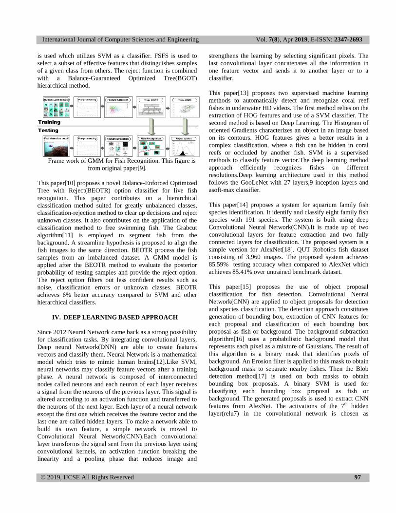
International Journal of Computer Sciences and Engineering Vol. 7(8), Apr 2019, E-ISSN: 2347-2693
© 2019, IJCSE All Rights Reserved 97
is used which utilizes SVM as a classifier. FSFS is used to
select a subset of effective features that distinguishes samples
of a given class from others. The reject function is combined
with a Balance-Guaranteed Optimized Tree(BGOT)
hierarchical method.
Frame work of GMM for Fish Recognition. This figure is
from original paper[9].
This paper[10] proposes a novel Balance-Enforced Optimized
Tree with Reject(BEOTR) option classifier for live fish
recognition. This paper contributes on a hierarchical
classification method suited for greatly unbalanced classes,
classification-rejection method to clear up decisions and reject
unknown classes. It also contributes on the application of the
classification method to free swimming fish. The Grabcut
algorithm[11] is employed to segment fish from the
background. A streamline hypothesis is proposed to align the
fish images to the same direction. BEOTR process the fish
samples from an imbalanced dataset. A GMM model is
applied after the BEOTR method to evaluate the posterior
probability of testing samples and provide the reject option.
The reject option filters out less confident results such as
noise, classification errors or unknown classes. BEOTR
achieves 6% better accuracy compared to SVM and other
hierarchical classifiers.
IV. DEEP LEARNING BASED APPROACH
Since 2012 Neural Network came back as a strong possibility
for classification tasks. By integrating convolutional layers,
Deep neural Network(DNN) are able to create features
vectors and classify them. Neural Network is a mathematical
model which tries to mimic human brains[12].Like SVM,
neural networks may classify feature vectors after a training
phase. A neural network is composed of interconnected
nodes called neurons and each neuron of each layer receives
a signal from the neurons of the previous layer. This signal is
altered according to an activation function and transferred to
the neurons of the next layer. Each layer of a neural network
except the first one which receives the feature vector and the
last one are called hidden layers. To make a network able to
build its own feature, a simple network is moved to
Convolutional Neural Network(CNN).Each convolutional
layer transforms the signal sent from the previous layer using
convolutional kernels, an activation function breaking the
linearity and a pooling phase that reduces image and
strengthens the learning by selecting significant pixels. The
last convolutional layer concatenates all the information in
one feature vector and sends it to another layer or to a
classifier.
This paper[13] proposes two supervised machine learning
methods to automatically detect and recognize coral reef
fishes in underwater HD videos. The first method relies on the
extraction of HOG features and use of a SVM classifier. The
second method is based on Deep Learning. The Histogram of
oriented Gradients characterizes an object in an image based
on its contours. HOG features gives a better results in a
complex classification, where a fish can be hidden in coral
reefs or occluded by another fish. SVM is a supervised
methods to classify feature vector.The deep learning method
approach efficiently recognizes fishes on different
resolutions.Deep learning architecture used in this method
follows the GooLeNet with 27 layers,9 inception layers and
asoft-max classifier.
This paper[14] proposes a system for aquarium family fish
species identification. It identify and classify eight family fish
species with 191 species. The system is built using deep
Convolutional Neural Network(CNN).It is made up of two
convolutional layers for feature extraction and two fully
connected layers for classification. The proposed system is a
simple version for AlexNet[18]. QUT Robotics fish dataset
consisting of 3,960 images. The proposed system achieves
85.59% testing accuracy when compared to AlexNet which
achieves 85.41% over untrained benchmark dataset.
This paper[15] proposes the use of object proposal
classification for fish detection. Convolutional Neural
Network(CNN) are applied to object proposals for detection
and species classification. The detection approach constitutes
generation of bounding box, extraction of CNN features for
each proposal and classification of each bounding box
proposal as fish or background. The background subtraction
algorithm[16] uses a probabilistic background model that
represents each pixel as a mixture of Gaussians. The result of
this algorithm is a binary mask that identifies pixels of
background. An Erosion filter is applied to this mask to obtain
background mask to separate nearby fishes. Then the Blob
detection method[17] is used on both masks to obtain
bounding box proposals. A binary SVM is used for
classifying each bounding box proposal as fish or
background. The generated proposals is used to extract CNN
features from AlexNet. The activations of the 7th
hidden
layer(relu7) in the convolutional network is chosen as

International Journal of Computer Sciences and Engineering Vol. 7(8), Apr 2019, E-ISSN: 2347-2693
© 2019, IJCSE All Rights Reserved 98
features.
Abstract view of the CNN architecture.This figure is
taken from paper[14]
A novel technique based on convolutional neural networks is
proposed in this paper[19] for fish classification.The noise in
the dataset are first removed.Image pre-processing is done
using gaussian Blurring,Morphological operations,Otsu’s
thresholding and Pyramid Mean Shifting.A grey level
histogram is created from the gray scale image for noise
removal.the outline of the fish object is obtained using
Pyramid Mean shifting with the kernel function k.The
enhanced image is feed to CNN for the classification of Fish
Species.This method gives an accuracy of 96.29%.
V. CONCLUSION
This survey paper discuss various types of approach for fish
recognition. Various techniques for image pre-processing is
discussed. Fish recognition using low level features,
hierarchical classification and deep learning is
discussed.Features has to be enhanced for larger dataset and
also to obtain 100% accuracy.
REFERENCES
[1] W. Rouse. Population dynamics of barnacles in the intertidal zone.
Marine Biology Research Experiment,2007
[2] P. Brehmer, T. Do Chi, and D. Mouillot.Amphidromous fish school migration revealed by combining fixed sonar monitoring (horizontalbeaming) with fishing data. Journal of Experimental Marine Biology and Ecology, 334:139–150, 2006
[3] D.-J.Lee,R.B.Schoenberger,D.Shiozawa,X.Xu,P.Zhan,Contour matching for a fish recognition and migration-monitoring system,in:OpticsEast,International Society for Optics and Photonics,2004,pp.37–48.
[4] .C. Pornpanomchai, B. Lurstwut, P. Leerasakultham, W. Kitiyanan, ―Shape and Texture based fish image recognition system‖, Kasetsart J. (Nat. Sci.) 47 : 624 - 634 (2013)
[5] C.Spampinato,D.Giordano,R.DiSalvo,Y.-H.J.Chen-urger,R.B.Fisher,G. Nadarajan,‖Automatic fish classification for underwater species behavior understanding‖, in:Proceedings of the FirstACM InternationalWorkshop on Analysis and Retrieval of Tracked Events and MotioninImageryStreams,ACM, Firenze,Italy,2010,pp.45–50.
[6] K.A. Mutasem, B.O. Khairuddin, N. Shahrulazman and A. Ibrahim . ―Fish Recognition Based on Robust Features Extraction from color Texture Measurements Using Back Propagation Classifier ‖
[7] N J C Strachan ,‖Recognition of fish species by colour and shape‖,ImageVis.Comput. 11(1)(1993)2-10
[8] 8.P.X.Huang,B.J.Boom,R.B.Fisher,‖Underwater live fish recognition using a balance-guaranteed optimized tree‖,in:ComputerVision–ACCV2012,Springer, Daejeon, Korea,2013,pp.422–433.
[9] .P.X.Huang,B.J.Boom,R.B.Fisher,‖Gmm improves the rejectoption in hierarchical classification for fishrecognition‖,in:2014IEEEWinter ConferenceonApplicationsofcomputerVision(WACV),IEEE,SteamboatSpringsCO.,USA,2014,pp.371–376.
[10] Phoenix X. Huang,Xuan.Huang,Bastiaan J. Boom,‖Hierarchical classification with reject option for live fish recognition‖
[11] C. Rother, V. Kolmogorov, and A. Blake,‖Grabcut - interactive foreground extraction using iterated graph cuts," ACM Transactions on Graph-ics (SIGGRAPH), August 2004.
[12] Atkinson, Peter M. et TATNALL, A. R. L. Introduction neural networks in remote sensing. International Journal of remote sensing, 1997, vol. 18, no 4, p.699-709.
[13] Sébastien Villon, Marc Chaumont, Gérard Subsol, Sébastien Villéger, Thomas Claverie and David Mouillot,‖Coral reef fish detection and recognition in underwater videos by supervised machine learning : Comparison between Deep Learning and HOG+SVM methods ―
[14] .Nour Eldeen M. Khalifa , Mohamed Hamed N. Taha and Aboul Ella Hassanien,‖Aquarium Family Fish Species Identification System Using Deep Neural Networks ―
[15] .Jonas Jager,Erik Rodner,Joachim Denzler,Viviane Wo and Klaus Fricke-Neuderth ,‖SeaCLEF 2016: Object proposal classification for fish detection in underwater videos‖
[16] Chris Stau_er and W. Eric L. Grimson. Adaptive background mixture models for real-time tracking. In 1999 Conference on Computer Vision and Pattern Recognition (CVPR '99), 23-25 June 1999, Ft. Collins, CO, USA, pages 2246{2252,1999.
[17] Satoshi Suzuki and Keiichi Abe,‖ Topological structural analysis of digitized binary images by border following. Computer Vision‖, Graphics, and Image Processing,30(1):32{46, 1985.
[18] Alex Krizhevsky, Ilya Sutskever, and Geo_rey E. Hinton,‖ Imagenet classification with deep convolutional neural networks. In F. Pereira, C.J.C. Burges, L. Bottou and K.Q. Weinberger, editors, Advances in Neural Information Processing Systems 25, pages 1097{1105. Curran Associates, Inc., 2012.
[19] .Dhruv Rathi, Sushant Jain and Dr. S. Indu,‖ Underwater Fish Species Classification using Convolutional Neural Network and Deep Learning ―
AUTHORS PROFILE R.FATHIMA SYREEN Research Scholar,Sarah Tucker
college,M.S University,Tirunelveli.Also working as
Assistant Professor in the Department of Computer
Applications,Sadakathullah Appa College.
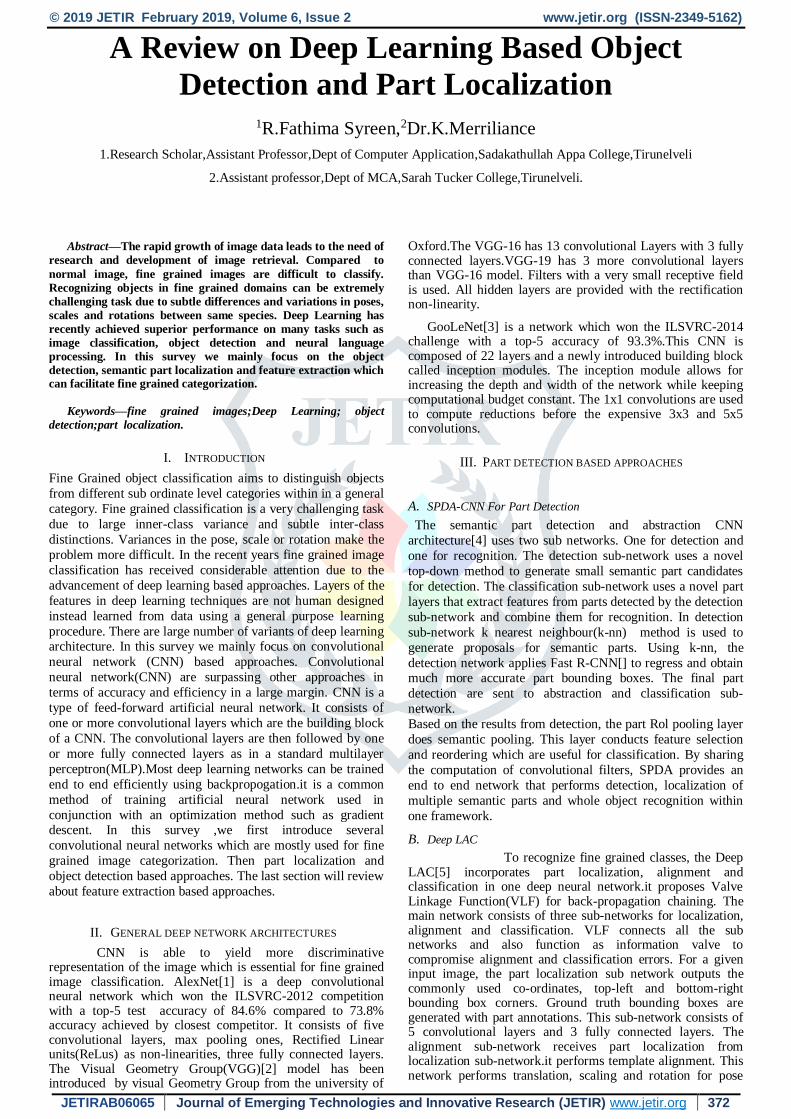
© 2019 JETIR February 2019, Volume 6, Issue 2 www.jetir.org (ISSN-2349-5162)
JETIRAB06065 Journal of Emerging Technologies and Innovative Research (JETIR) www.jetir.org 372
A Review on Deep Learning Based Object
Detection and Part Localization
1R.Fathima Syreen,2Dr.K.Merriliance
1.Research Scholar,Assistant Professor,Dept of Computer Application,Sadakathullah Appa College,Tirunelveli
2.Assistant professor,Dept of MCA,Sarah Tucker College,Tirunelveli.
Abstract—The rapid growth of image data leads to the need of
research and development of image retrieval. Compared to
normal image, fine grained images are difficult to classify.
Recognizing objects in fine grained domains can be extremely
challenging task due to subtle differences and variations in poses,
scales and rotations between same species. Deep Learning has
recently achieved superior performance on many tasks such as
image classification, object detection and neural language
processing. In this survey we mainly focus on the object
detection, semantic part localization and feature extraction which can facilitate fine grained categorization.
Keywords—fine grained images;Deep Learning; object
detection;part localization.
I. INTRODUCTION
Fine Grained object classification aims to distinguish objects
from different sub ordinate level categories within in a general
category. Fine grained classification is a very challenging task
due to large inner-class variance and subtle inter-class
distinctions. Variances in the pose, scale or rotation make the
problem more difficult. In the recent years fine grained image
classification has received considerable attention due to the
advancement of deep learning based approaches. Layers of the
features in deep learning techniques are not human designed
instead learned from data using a general purpose learning
procedure. There are large number of variants of deep learning architecture. In this survey we mainly focus on convolutional
neural network (CNN) based approaches. Convolutional
neural network(CNN) are surpassing other approaches in
terms of accuracy and efficiency in a large margin. CNN is a
type of feed-forward artificial neural network. It consists of
one or more convolutional layers which are the building block
of a CNN. The convolutional layers are then followed by one
or more fully connected layers as in a standard multilayer
perceptron(MLP).Most deep learning networks can be trained
end to end efficiently using backpropogation.it is a common
method of training artificial neural network used in
conjunction with an optimization method such as gradient descent. In this survey ,we first introduce several
convolutional neural networks which are mostly used for fine
grained image categorization. Then part localization and
object detection based approaches. The last section will review
about feature extraction based approaches.
II. GENERAL DEEP NETWORK ARCHITECTURES
CNN is able to yield more discriminative representation of the image which is essential for fine grained image classification. AlexNet[1] is a deep convolutional neural network which won the ILSVRC-2012 competition with a top-5 test accuracy of 84.6% compared to 73.8% accuracy achieved by closest competitor. It consists of five convolutional layers, max pooling ones, Rectified Linear units(ReLus) as non-linearities, three fully connected layers. The Visual Geometry Group(VGG)[2] model has been introduced by visual Geometry Group from the university of
Oxford.The VGG-16 has 13 convolutional Layers with 3 fully connected layers.VGG-19 has 3 more convolutional layers than VGG-16 model. Filters with a very small receptive field is used. All hidden layers are provided with the rectification non-linearity.
GooLeNet[3] is a network which won the ILSVRC-2014 challenge with a top-5 accuracy of 93.3%.This CNN is composed of 22 layers and a newly introduced building block called inception modules. The inception module allows for increasing the depth and width of the network while keeping computational budget constant. The 1x1 convolutions are used to compute reductions before the expensive 3x3 and 5x5 convolutions.
III. PART DETECTION BASED APPROACHES
A. SPDA-CNN For Part Detection
The semantic part detection and abstraction CNN
architecture[4] uses two sub networks. One for detection and
one for recognition. The detection sub-network uses a novel
top-down method to generate small semantic part candidates
for detection. The classification sub-network uses a novel part
layers that extract features from parts detected by the detection
sub-network and combine them for recognition. In detection
sub-network k nearest neighbour(k-nn) method is used to
generate proposals for semantic parts. Using k-nn, the
detection network applies Fast R-CNN[] to regress and obtain much more accurate part bounding boxes. The final part
detection are sent to abstraction and classification sub-
network.
Based on the results from detection, the part Rol pooling layer
does semantic pooling. This layer conducts feature selection
and reordering which are useful for classification. By sharing
the computation of convolutional filters, SPDA provides an
end to end network that performs detection, localization of
multiple semantic parts and whole object recognition within
one framework.
B. Deep LAC
To recognize fine grained classes, the Deep LAC[5] incorporates part localization, alignment and classification in one deep neural network.it proposes Valve Linkage Function(VLF) for back-propagation chaining. The main network consists of three sub-networks for localization, alignment and classification. VLF connects all the sub networks and also function as information valve to compromise alignment and classification errors. For a given input image, the part localization sub network outputs the commonly used co-ordinates, top-left and bottom-right bounding box corners. Ground truth bounding boxes are generated with part annotations. This sub-network consists of 5 convolutional layers and 3 fully connected layers. The alignment sub-network receives part localization from localization sub-network.it performs template alignment. This network performs translation, scaling and rotation for pose
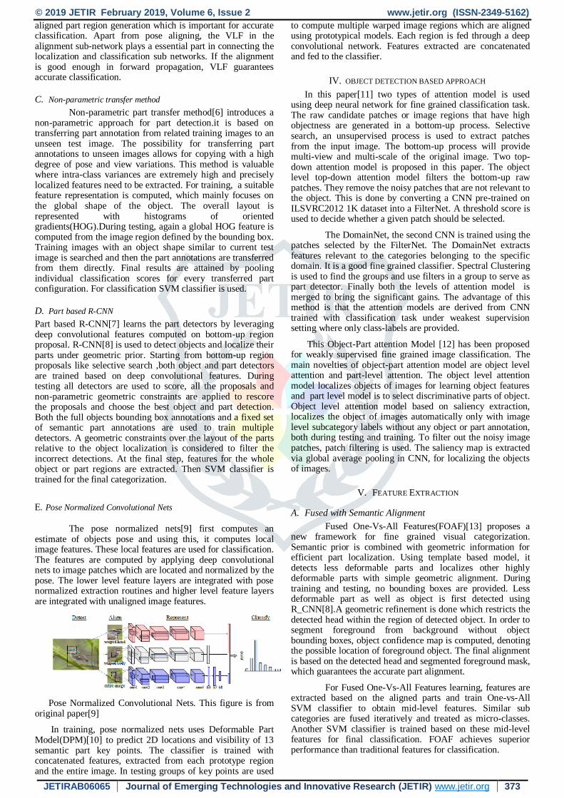
© 2019 JETIR February 2019, Volume 6, Issue 2 www.jetir.org (ISSN-2349-5162)
JETIRAB06065 Journal of Emerging Technologies and Innovative Research (JETIR) www.jetir.org 373
aligned part region generation which is important for accurate classification. Apart from pose aligning, the VLF in the alignment sub-network plays a essential part in connecting the localization and classification sub networks. If the alignment is good enough in forward propagation, VLF guarantees accurate classification.
C. Non-parametric transfer method
Non-parametric part transfer method[6] introduces a non-parametric approach for part detection.it is based on transferring part annotation from related training images to an unseen test image. The possibility for transferring part annotations to unseen images allows for copying with a high degree of pose and view variations. This method is valuable where intra-class variances are extremely high and precisely localized features need to be extracted. For training, a suitable feature representation is computed, which mainly focuses on the global shape of the object. The overall layout is represented with histograms of oriented gradients(HOG).During testing, again a global HOG feature is computed from the image region defined by the bounding box. Training images with an object shape similar to current test image is searched and then the part annotations are transferred from them directly. Final results are attained by pooling individual classification scores for every transferred part configuration. For classification SVM classifier is used.
D. Part based R-CNN
Part based R-CNN[7] learns the part detectors by leveraging deep convolutional features computed on bottom-up region proposal. R-CNN[8] is used to detect objects and localize their parts under geometric prior. Starting from bottom-up region proposals like selective search ,both object and part detectors are trained based on deep convolutional features. During testing all detectors are used to score, all the proposals and non-parametric geometric constraints are applied to rescore the proposals and choose the best object and part detection. Both the full objects bounding box annotations and a fixed set of semantic part annotations are used to train multiple detectors. A geometric constraints over the layout of the parts relative to the object localization is considered to filter the incorrect detections. At the final step, features for the whole object or part regions are extracted. Then SVM classifier is trained for the final categorization.
Pose Normalized Convolutional Nets
The pose normalized nets[9] first computes an estimate of objects pose and using this, it computes local image features. These local features are used for classification. The features are computed by applying deep convolutional nets to image patches which are located and normalized by the pose. The lower level feature layers are integrated with pose normalized extraction routines and higher level feature layers are integrated with unaligned image features.
Pose Normalized Convolutional Nets. This figure is from original paper[9]
In training, pose normalized nets uses Deformable Part Model(DPM)[10] to predict 2D locations and visibility of 13 semantic part key points. The classifier is trained with concatenated features, extracted from each prototype region and the entire image. In testing groups of key points are used
to compute multiple warped image regions which are aligned using prototypical models. Each region is fed through a deep convolutional network. Features extracted are concatenated and fed to the classifier.
IV. OBJECT DETECTION BASED APPROACH
In this paper[11] two types of attention model is used using deep neural network for fine grained classification task. The raw candidate patches or image regions that have high objectness are generated in a bottom-up process. Selective search, an unsupervised process is used to extract patches from the input image. The bottom-up process will provide multi-view and multi-scale of the original image. Two top-down attention model is proposed in this paper. The object level top-down attention model filters the bottom-up raw patches. They remove the noisy patches that are not relevant to the object. This is done by converting a CNN pre-trained on ILSVRC2012 1K dataset into a FilterNet. A threshold score is used to decide whether a given patch should be selected.
The DomainNet, the second CNN is trained using the patches selected by the FilterNet. The DomainNet extracts features relevant to the categories belonging to the specific domain. It is a good fine grained classifier. Spectral Clustering is used to find the groups and use filters in a group to serve as part detector. Finally both the levels of attention model is merged to bring the significant gains. The advantage of this method is that the attention models are derived from CNN trained with classification task under weakest supervision setting where only class-labels are provided.
This Object-Part attention Model [12] has been proposed for weakly supervised fine grained image classification. The main novelties of object-part attention model are object level attention and part-level attention. The object level attention model localizes objects of images for learning object features and part level model is to select discriminative parts of object. Object level attention model based on saliency extraction, localizes the object of images automatically only with image level subcategory labels without any object or part annotation, both during testing and training. To filter out the noisy image patches, patch filtering is used. The saliency map is extracted via global average pooling in CNN, for localizing the objects of images.
V. FEATURE EXTRACTION
A. Fused with Semantic Alignment
Fused One-Vs-All Features(FOAF)[13] proposes a new framework for fine grained visual categorization. Semantic prior is combined with geometric information for efficient part localization. Using template based model, it detects less deformable parts and localizes other highly deformable parts with simple geometric alignment. During training and testing, no bounding boxes are provided. Less deformable part as well as object is first detected using R_CNN[8].A geometric refinement is done which restricts the detected head within the region of detected object. In order to segment foreground from background without object bounding boxes, object confidence map is computed, denoting the possible location of foreground object. The final alignment is based on the detected head and segmented foreground mask, which guarantees the accurate part alignment.
For Fused One-Vs-All Features learning, features are extracted based on the aligned parts and train One-vs-All SVM classifier to obtain mid-level features. Similar sub categories are fused iteratively and treated as micro-classes. Another SVM classifier is trained based on these mid-level features for final classification. FOAF achieves superior performance than traditional features for classification.

© 2019 JETIR February 2019, Volume 6, Issue 2 www.jetir.org (ISSN-2349-5162)
JETIRAB06065 Journal of Emerging Technologies and Innovative Research (JETIR) www.jetir.org 374
B. Subset Feature learning
Subset Feature learning[14] consists of two main parts. It proposes a subset learning system, which first clusters visually similar classes and then learns deep convolutional neural network for each subset. A progressive transfer learning system also been proposed to learn domain-generic convolutional feature extractor. Applying Linear Discriminant Analysis(LDA) to fc6 features to reduce their dimensionality, visually similar species are clustered into k subsets. A separate CNN is attained for each of the k pre-clustered subsets.
To select most relevant subset is to train a separate CNN based subset selector(SCNN).Using the output from the pre-clustering as the class labels, SCNN is trained by changing the softmax layer fc8 to make it have K outputs. As with the previously trained CNNs, the weights of SCNN are trained via back propagation.
C. Selective Convolutional Descriptor
In an unsupervised methodology of feature extraction
Selective Convolutional Descriptor Aggregation(SCDA)[15]
meet the challenges of automatically localizes the main
object in fine grained images. A pretrained CNN model first
extracts convolution activations for an input image. A
Multiscale Orderless Pooling (MOP) CNN first extract CNN
activations and perform VLAD pooling to determine the
useful part of the activations. These useful descriptors are
then aggregated using sum-pooled convolutional features on
the last convolutional layer which outperforms the traditional methods like PCA(Principle Component Analysis). In
SCDA, the preliminary step is getting pool5 which refers to
the activations of the max-pooled last convolutional layer. To
obtain a useful deep descriptors and removing background
noise, aggregation map(A) is used. Then following this, mask
map(M) of the same size as A is obtained. In order to resize
it, bicubic interpolation is used whose size is same as input
image.
D. Bilinear CNN
Bilinear Model[16] consists of two independent
features combined with an outer product. A feature function
takes as input, an image I and a location L and outputs a
feature of size CxD. Generally locations can include position
and scale. The feature outputs are combined with an outer
product using the matrix outer product. To obtain an image
descriptor, the pooling function aggregates the bilinear features across all locations in the image.
Bilinear CNN model. This figure is from original paper[16]
A natural candidate for the feature function f is a
Convolutional neural network which consists of a hierarchy
of convolutional and pooling layers. Two different CNNs pretrained on ImageNet datasets are used. By pretraining,
bilinear deep network will benefit from additional training
data in the cases of domain specific data scarcity. The
variants of outer product representations are very effective at
various texture, fine grained and scene recognition tasks.
E. Refining Deep Convolutional Features
Incorporating multi-scale image recognition using Fisher
Vector(FV) CNN is proposed in Refining deep convolutional
features[17].It is based on an unsupervised manner in
extracting features. A non parametric feature weighting
method is proposed on the basis of refining convolutional
descriptors to boost the performance. To generate multiscale
information pooling of feature tensors of the last convolutional layers with ReLu activation in a CNN is
achieved using different pooling window sizes. No object
bounding box and part annotations are used during training
and testing times. Only image labels are used. Networks like
VGG-16 and AlexNet are used
Table-1 Architecture and accuracy between different methods
Method
Architecture Accuracy(%)
Part-based R-CNN
Pose Normalized Nets
Deep LAC
SPDA-CNN
Two-level attention Model
Bilinear CNN
Subset Feature Learning
Fused One Vs-All Feature
AlexNet
AlexNet
AlexNet
VGGNET
AlexNet
VGGnet
AlexNet
VGGNet
76.4
75.7
84.10
85.14
69.7
77.2
77.5
84.63
VI. CONCLUSION
This paper surveys some recent programs in deep learning based fine grained object detection and part localization. Several common convolutional neural networks are introduced first, including AlexNet, VGGNet and GooLeNet. They can be directly adapted to fine grained image classification. Since there are large intra class variance and small inter class variance in fine grained image classification, many common approaches resort to deep learning technology for object detection. While some approaches integrate the part localization into the deep learning framework, since subtle differences of visually similar fine grained objects exists in local parts. Some Fine grained categorization approaches also combine feature extraction to gain more classification capability and accuracy for fine grained images.
REFERENCES
[1]. Y. LeCun, B. Boser, J. S. Denker, D. Henderson, R. E.Howard, W.
Hubbard, L. D. Jackel.,”Backpropagation applied to handwritten zip
code recognition.” Neural Computation,
[2]. K. Simonyan, A. Zisserman.”Very deep convolutional networks for
large-scale image recognition.”, arXiv:1409.1556,2014 [3]. C. Szegedy, W. Liu, Y. Q. Jia, P. Sermanet, S. Reed, D.Anguelov,
D. Erhan, V. Vanhoucke, A. Rabinovich,”Going deeper with
convolutions.” In Proceedings of IEEE Conference on Computer Vision and
Pattern Recognition, IEEE, Boston, USA, pp. 1–9, 2014.
[4]. H. Zhang et al., “SPDA-CNN: Unifying semantic part detection and
abstraction for fine-grained recognition,” in Proc. IEEE Conf.
Comput Vis. Pattern Recognit. (CVPR), Jun. 2016, pp. 1143–1152.
[5]. D. Lin, X. Shen, C. Lu, and J. Jia, “Deep LAC: Deep localization,
alignment and classification for fine-grained recognition,” in Proc.
IEEE Conf. Comput. Vis. Pattern Recognit., Jun. 2015, pp. 1666– 1674.
[6]. C. Göering, E. Rodner, A. Freytag, and J. Denzler, “Nonparametric part
transfer for fine-grained recognition,” in Proc. IEEE Conf.
Comput.Vis Pattern Recognit. (CVPR), Jun. 2014, pp. 2489–2496.
[7]. N. Zhang, J. Donahue, R. Girshick, and T. Darrell, “Part-based R-CNNs
for fine-grained category detection,” in Computer Vision—
ECCV. Cham, Switzerland: Springer, 2014, pp. 834–849.

© 2019 JETIR February 2019, Volume 6, Issue 2 www.jetir.org (ISSN-2349-5162)
JETIRAB06065 Journal of Emerging Technologies and Innovative Research (JETIR) www.jetir.org 375
[8]. W. Zaremba, I. Sutskever, and O. Vinyals, “Recurrent neural Network
regularization,” ArXiv:abs/1409.2329, 2014.
[9]. S. Branson, G. Van Horn, S. Belongie, and P. Perona, “Bird species
categorization using pose normalized deep convolutional nets,” in
Proc.BMVC, Jun. 2014.
[10]. S. Branson, O. Beijbom and S. Belongie,” Efficient large-scalestructured
learning.” in Proceedings of IEEE Conference on Computer Vision and
Pattern Recognition, IEEE, Portland, USA, pp. 1806–1813, 2013.
.
[11]. T. Xiao, Y. Xu, K. Yang, J. Zhang, Y. Peng, and Z. Zhang, “The
application of two-level attention models in deep Convolutional
neural network for fine-grained image classification,” in Proc. IEEE
Conf. Comput. Vis. Pattern Recognit., Jun. 2014, pp. 842–850.
[12]. Yuxin Peng , Xiangteng He, and Junjie Zhao, “Object-Part Attention
Model for Fine-Grained Image Classification”,IEEE Trans. Image
Process., vol. 27, no. 3,Mar. 2018.
[13]. X. Zhang, H. Xiong, W. Zhou, and Q. Tian, “Fused one-vs-all Features
with semantic alignments for fine-grained visual categorization,” IEEE
Trans. Image Process., vol. 25, no. 2, pp. 878–892, Feb. 2016.
[14]. Z. Ge, C. McCool, C. Sanderson, and P. Corke, “Subset feature learning
for fine-grained category classification,” in Proc. IEEE Conf. Comput
Vis. Pattern Recognit. Workshops, Jun. 2015, pp. 46–52.
[15]. X.S. Wei, J.H Luo and J.X. Wu, “Selective convolutional descriptor
aggregation for fine-grained image retrieval”, Xiv:1604.04994,2016
[16]. T.-Y. Lin, A. RoyChowdhury, and S. Maji, “Bilinear CNN models for
fine-grained visual recognition,” in Proc. IEEE Int. Conf.
Comput. Vis.,Dec. 2015, pp. 1449–1457.
[17]. Weixia Zhang,Jia Yan,Wenxuan Shi,Tianpeng Feng,Dexiang Deng”
Refining deep convolutional features for improving fine-grained
image recognition”
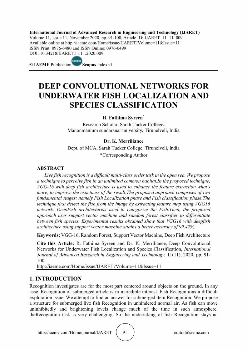
http://iaeme.com/Home/journal/IJARET 91 [email protected]
International Journal of Advanced Research in Engineering and Technology (IJARET) Volume 11, Issue 11, November 2020, pp. 91-100, Article ID: IJARET_11_11_009 Available online at http://iaeme.com/Home/issue/IJARET?Volume=11&Issue=11 ISSN Print: 0976-6480 and ISSN Online: 0976-6499 DOI 10.34218/IJARET.11.11.2020.009 :
© IAEME Publication Indexed Scopus
DEEP CONVOLUTIONAL NETWORKS FOR UNDERWATER FISH LOCALIZATION AND
SPECIES CLASSIFICATION R. Fathima Syreen*
Research Scholar, Sarah Tucker College, Manonmanium sundaranar university Tirunelveli, India ,
Dr. K. Merriliance Dept. of MCA, Sarah Tucker College, Tirunelveli, India
*Corresponding Author
ABSTRACT Live fish recognition is a difficult multi-class order task in the open sea. We propose
a technique to perceive fish in an unlimited common habitat.In the proposed technique, VGG-16 with deep fish architecture is used to enhance the feature extraction what's more, to improve the exactness of the result.The proposed approach comprises of two fundamental stages; namely Fish Localization phase and Fish classification phase.The technique first detect the fish from the image by extracting feature map using VGG16
network. DeepFish architectureis used to categorize the Fish.Then, the proposed approach uses support vector machine and random forest classifier to differentiate
between fish species. Experimental results obtained show that VGG16 with deepfish architecture using support vector machine attains a better accuracy of 99.47%.
Keywords: VGG-16, Random Forest, Support Vector Machine, Deep Fish Architecture Cite this Article: R. Fathima Syreen and Dr. K. Merriliance, Deep Convolutional
Networks for Underwater Fish Localization and Species Classification, International Journal of Advanced Research in Engineering and Technology, 11(11), 2020, pp. 91-100. http://iaeme.com/Home/issue/IJARET?Volume=11&Issue=11
1. INTRODUCTION Recognition investigates are for the most part centered around objects on the ground. In any case, Recognition of submerged article is in incredible interest. Fish Recognitions a difficult exploration issue. We attempt to find an answer for submerged item Recognition. We propose a structure for submerged live fish Recognition in unhindered normal air. As fish can move
uninhibitedly and brightening levels change much of the time in such atmosphere, theRecognition task is very challenging. So the undertaking of fish Recognition stays an

Deep Convolutional Networks for Underwater Fish Localization and Species Classification
http://iaeme.com/Home/journal/IJARET 92 [email protected]
extraordinary exploration issue. Article identification which is one of the significant applications in the field of PC vision has been the focal point of examination, and convolution
neural system has made incredible improvement in object discovery. Article discovery is advancing from the single item Recognition to the multi-object recognition. The initial one
recognizes a solitary article from a image, it very well may be said that it is an issue of characterization, and the later isn't just can distinguish all the articles in a image, however finds the specific area of the articles. Intricacy emerges in light of the fact that discovery requires the precise limitation of articles and arrangement of items
Over the most recent couple of years, object order and location capacities have fundamentally improved because of advances in profound learning and convolutional networks. This improvement isn't just because of the consequence of all the more remarkable equipment, bigger datasets and greater models, yet for the most part a result of new thoughts, calculations
and improved system structures. Present day ways to deal with object Recognition utilize profound learning techniques. Convolutional neural systems (CNNs) make ground-breaking and for the most part precise suppositions about the idea of images. CNNs have many less associations and boundaries contrasted with standard feed forward neural systems with likewise measured layers thus they are simpler to prepare. The most basic technique of improving the
exhibition of profound neural systems is by expanding their size. This incorporates both expanding the profundity just as its width. In this paper, we propose two CNN systems to limit
the item and to classify the article. The system comprises of two primary modules: 1) confinement net and 2) characterization net. For restriction net, we calibrated 16-layer VGG organize and for order net, we utilize a DeepFish design. train a profound recognition Weorganize VGG16 and concentrates highlight map utilizing pooling layer'pool2'. At that point highlights gained from DeepFish design are given to SVM and Random woods classifier for arrangement task.
2. RELATED WORKS The problem of fine grained Recognition in ordering objects which look fundamentally the same as and contrast just for unobtrusive subtleties have been as of late tended to by the PC
vision, AI and interactive media mainstream researchers. In [6] uses highlight extraction utilizing SIFT and SURF calculation followed via programmed characterization utilizing SVM classifier. It brings about exactness of 94.44% utilizing SIFT, just 69.57% utilizing SURF calculation in the interim SVM beats than KNN and ANN. Creators in [16] proposed a strategy
to perceive fish in an unhindered common habitat recorded by submerged cameras. This technique separates 66 kinds of highlights, which are a mix of shading, shape and surface properties from various pieces of the fish and diminish the component measurements with
Forward Sequential Feature Selection determination (FSFS) technique ology. The chose highlights of the FSFS are utilized by a SVM classifier. A Balance-Guaranteed Optimized Tree (BGOT) has been applied so as to control the blunder aggregation in progressive grouping and, in this way, accomplish better execution. A BGOT of 10 fish species is naturally built utilizing the interclass similitudes and a heuristic strategy. The proposed BGOT based various leveled arrangement strategy accomplished around 4% better exactness contrasted with cutting edge techniques on a live fish image dataset.
Earlier fish Recognition explores are mostly limited to obliged situations. Leeetal[27] utilized form coordinating to perceive fish in the fish tanks.Strachanetal [21 23] utilized –
shading and shape descriptors to perceive fish shipped along a transport line underneath an advanced camera.Larsenetal[28] determined shape and surface highlights from an appearance model, classified with LDAand tried on a dataset containing 108 images of three fish species under compelled condition(caught from the ocean), accomplishing an accuracy of 76%.There

R. Fathima Syreen and Dr. K. Merriliance
http://iaeme.com/Home/journal/IJARET 93 [email protected]
are additionally explores completed on submerged live fish.Spampinatoetal [ ] consolidated surface highlights and shape includes and tried on a database containing 360 images frequently
fish species, achieving a normal exactness of 92%.Huangetal [17] introduced a Balance-Enforced Optimized Tree with Reject Option(BEOTR)algorithm for live fish Recognition with dismissal alternative. They did an examination on a dataset containing 24150 physically named fish images of 15 fish species gathered from south Taiwan Sea. Then in [29], they further utilized GMM to improve the oddball choice in progressive order. With BGOT and GMM they got a normal accuracy of 65% on a bigger dataset containing 24,150 images of 15 species.
3. PROPOSED FRAMEWORK Item areas of images are gotten through Localisation Net and afterward we utilize DeepFish engineering to arrange the article as shown in figure 1. As of late, convolutional neural systems
(CNNs) have been incorporated into number of visual Recognition frameworks in a wide assortment of spaces. Rather than more conventional item Recognition strategies which register hand-built highlights on images as an underlying pre-processing step, the quality of the CNN lies in their capacity to take in discriminative highlights from crude information inputs (e.g., image pixels). CNNs were advocated by LeCun and associates who originally utilized such
models to conventional article Recognition and to digit Recognition task. In object acknowledgment, include extraction for the most part made out of a channel bank layer, a non-direct change, and a component pooling layer. A run of the mill convolutional neural systems (CNN) is such a framework that comprises of a few layers. A convolutional channel bank layer means to separate nearby examples. The motivation behind nonlinear preparing layer is to frame a non-direct complex model. The goal of highlight pooling layer is to diminish include maps goal. In Recent occasions, conventional article identification techniques have started to use profound CNNs and beat any contending approaches dependent on customary highlights.
Figure 1 Architecture of Proposed Framework
3.1. Fine Grained Fish Localization The LocalisationNet arrange takes as information a whole image. The system first procedures the entire image with a few convolutional (conv) and max pooling layers to deliver a conv include map. At that point a fixed-length include vector from the element map is separated in
the pooling layer. A productive preparing technique is proposed which exploits highlight sharing during preparing. Max-pooling layers has likewise been successfully utilized for
localization.Objectness map is characterized as a image where every pixel esteem demonstrates the likelihood that the pixel has a place with an intrigued object. CNN is a mainstream zone of examination inside the field of man-made brainpower and image order. It very well may be

Deep Convolutional Networks for Underwater Fish Localization and Species Classification
http://iaeme.com/Home/journal/IJARET 94 [email protected]
utilized to distinguish and characterize protests by essentially providing a PC program with enough information and set up this system to prepare itself so as to tackle the given
characterization issue. We separate profound convolutional highlights utilizing a VGG16 pre- prepared CNN model. To accomplish our particular area and create more discriminative
highlights, we tweak the pre-prepared CNN model. All the more explicitly, we utilize a 5-way fc3 layer (the last completely associated layer), rather than a 1000-way fc3 order layer as
appeared in Fig2. Past work in the field depends on applying channels to the images to isolate the fish from the foundation or hone the images by evacuating foundation commotion. The images from the dataset are separated from submerged cameras and contain commotion, so arranging these images is testing. As the Convolutional Neural Network (CNN) has shown solid discriminative power, we utilize the element maps in CNN to evaluate the nearness of fish species. Applying normal pooling on conv or pool we find that component maps acquires a image adequately speaking to the fish area. A large portion of highlight maps center around the
frontal area fish locale, despite the fact that there exist some component map with high enactment on the foundation. Subsequently, applying normal pooling on those element guides would stifle the actuation on foundation, in the interim assemble and feature the initiation on closer view area. VGG16 is a convolution neural net (CNN) engineering which is viewed as one of the brilliant vision model design till date. Most one of a kind thing about VGG16 is that as opposed to having countless hyper-boundary they concentrated on having convolution layers of 3x3 channel with a step 1 and consistently utilized same cushioning and maxpool layer of 2x2 channel of step 2. It follows this game plan of convolution and max pool layers reliably all through the entire design. At long last it has 2 FC(Fully Connected layers) trailed by a softmax for yield. The 16 in VGG16 alludes to it has 16 layers that have loads. This system is a really enormous system and it has around 138 million (approx) boundaries.
Figure 2 Architecture of VGG-16 for localizing fish species
When this CNN is tweaked, we extricate its pool highlight guides to make objectness map. The pool include speaks to the reactions of various convolutional channels on the article. As there are various pool layers in VGG-16 net, we break down the objectness map produced by various layers, e.g., pool2, pool3, pool4, pool5. Contrasted and the objectness map created by pool2 layer, the objectness maps produced by pool3 and pool4 have higher reaction on the foundation locales. Accordingly, it is more reasonable to utilize pool2 to produce the objectness map. To create the objectness map for a given image I, we initially resize it to measure 224×224, at that point feed it into the CNN to separate its pool2 include. The size of pool2 is 512×7×7. It uses the worldwide normal pooling in CNN for limiting fish of images, instead of just choosing the image patches pertinent to fish that have huge regions of foundation commotion.

R. Fathima Syreen and Dr. K. Merriliance
http://iaeme.com/Home/journal/IJARET 95 [email protected]
3.2. Fish ClassificationSubsequent to confining the fish from the given image,a profound fish architecture[1] is utilized for arrangement task as appeared in Fig 3.Deep design comprises of PCANet[2]. A convolution profound neural system (ConvNet) is one of the key segment of profound learning strategy utilized in image characterization. ConvNet are intended to perceive neighborhood designs. ConvNet comprises of a few phases that are teachable, stacked on head of one another which follow a directed classifier. The stages comprise of layers of a convolutional channel bank, a
nonlinear handling and an element pooling. The PCANet[2] contains three fundamental information handling components: fell PCA, paired hashing and square savvy histogram.
Furthermore, these components incorporate the three phases of PCANet: the initial two phases are of PCA convolution and the last yield stage is the blend of double hashing and square insightful histogram. Convolution layer of the ConvNet can be considered as the PCA falling and the Hashing and histogramming are utilized rather than the nonlinear preparing layer and highlight pooling layer. The phases that comprise of fell PCA can be expanded or diminished as and when requested by the issue. Principal Component Analysis (PCA) is very well known procedure of dimensionality reduction. Given an information with n measurements PCA is use to lessen the information to k measurement with least conceivable remaking mistake. In the wake of finishing PCANet process, every preparing test compares to an element vector. These highlights are then utilized for order task. For order task we utilize the Support Vector Machine (SVM) and Random Forest classifier.
Figure 3 DeepFish Architecture
3.2.1. SVM VS Random Forest An essential piece of AI is order and to anticipate what class our species has a place with. Information science gives a bounty of grouping calculations, for example, strategic relapse, bolster vector machine, guileless Bayes classifier, and choice trees. The Support Vector Machines (SVMs) is a Machine Learning (ML) calculation that is utilized for order. A SVM
takes care of the characterization issue by finding the best hyperplane that isolates all information purposes of one class from those of the other class.SVM calculation tries to expand
the edge around a hyperplane that isolates a positive class from a negative class. Mathematically, the SVM demonstrating calculation finds an ideal hyperplane with the
maximal edge to isolate two classes, which requires to take care of the streamlining issue, as appeared in conditions.

Deep Convolutional Networks for Underwater Fish Localization and Species Classification
http://iaeme.com/Home/journal/IJARET 96 [email protected]
where, I is the weight allotted to the preparation test xi. In the event that _i > 0, xi is known as a help vector. C is a guideline boundary used to compromise the preparation exactness and the model multifaceted nature so a prevalent speculation ability can be accomplished. K is a bit work, which is utilized to quantify the likeness between two examples.
Random Forest (RF) is a gathering learning technique that has been utilized for order and relapse. RF was created by Brieman. The strategy fills in as a lot of autonomous classifiers (normally choice trees), where every classifier picks a specific example in an informational collection, and afterward dominant part casting a ballot is considered to decide the last class name. RF has a few preferences over other learning techniques, however one of its imperative focal points is its power to clamor and overfitting. The arbitrary determination of highlights is
done at every hub split for developing the tree. Irregular Forests fabricates numerous characterization trees. To arrange another article from an information vector, put the info vector down every one of the trees in the backwoods. Each tree gives an order, and we state the tree "votes" for that class. The woodland picks the arrangement having the most votes (over all the trees in the timberland).The error rate of random forest depends on two things:
The correlation between any two trees in the forest. Increasing the correlation increases the forest error rate.
The strength of each individual tree in the forest. A tree with a low error rate is a strong classifier. Increasing the strength of the individual trees decreases the forest error rate.
4. EXPERIMENTAL RESULTS
Figure 4 Fish Species used in this experiment
4.1. Datasets The viability of the design are assessed utilizing the dataset made by fish images from
Fish4Knowledge (F4K) Project [30].This submerged live fish dataset is gained from a live video dataset caught from the vast ocean. The proposed approach was assessed utilizing 509 images of 5 fish species. The dataset was part into equal parts, one for training (484) and other for testing (25). The case of Fish Species are appeared in Fig 2.There are different sizes of fish images extending from about 20x20 to about 200x200 pixels. They are resized to same size. Images in the dataset change in orientation, scaling and position. They additionally shift in shading and textures. All the images are resized to 47x47 for Deep Fishnet.
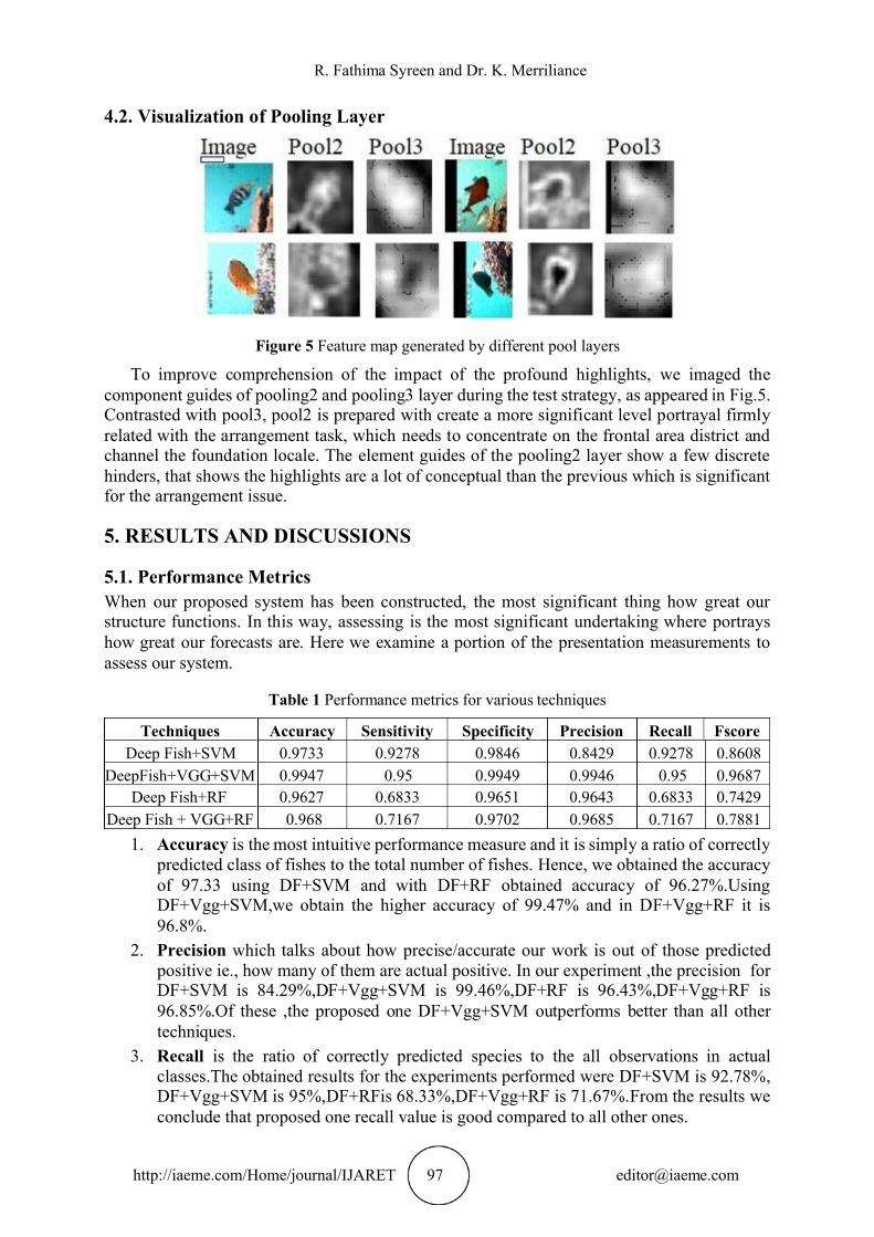
R. Fathima Syreen and Dr. K. Merriliance
http://iaeme.com/Home/journal/IJARET 97 [email protected]
4.2. Visualization of Pooling Layer
Figure 5 Feature map generated by different pool layers
To improve comprehension of the impact of the profound highlights, we imaged the component guides of pooling2 and pooling3 layer during the test strategy, as appeared in Fig.5. Contrasted with pool3, pool2 is prepared with create a more significant level portrayal firmly related with the arrangement task, which needs to concentrate on the frontal area district and channel the foundation locale. The element guides of the pooling2 layer show a few discrete hinders, that shows the highlights are a lot of conceptual than the previous which is significant for the arrangement issue.
5. RESULTS DISCUSSIONS AND
5.1. Performance Metrics When our proposed system has been constructed, the most significant thing how great our structure functions. In this way, assessing is the most significant undertaking where portrays how great our forecasts are. Here we examine a portion of the presentation measurements to assess our system.
Table 1 Performance metrics for various techniques
Techniques Accuracy Sensitivity Specificity Precision Recall Fscore Deep Fish+SVM 0.9733 0.9278 0.9846 0.8429 0.9278 0.8608
DeepFish+VGG+SVM 0.9947 0.95 0.9949 0.9946 0.95 0.9687 Deep Fish+RF 0.9627 0.6833 0.9651 0.9643 0.6833 0.7429
Deep Fish + VGG+RF 0.968 0.7167 0.9702 0.9685 0.7167 0.7881 1. is the most intuitive performance measure and it is simply a ratio of correctly Accuracypredicted class of fishes to the total number of fishes. Hence, we obtained the accuracy
of 97.33 using DF+SVM and with DF+RF obtained accuracy of 96.27%.Using DF+Vgg+SVM,we obtain the higher accuracy of 99.47% and in DF+Vgg+RF it is
96.8%. 2. which talks about how precise/accurate our work is out of those predicted Precision positive ie., how many of them are actual positive. In our experiment ,the precision for
DF+SVM is 84.29%,DF+Vgg+SVM is 99.46%,DF+RF is 96.43%,DF+Vgg+RF is 96.85%.Of these ,the proposed one DF+Vgg+SVM outperforms better than all other techniques.
3. is the ratio of correctly predicted species to the all observations in actual Recallclasses.The obtained results for the experiments performed were DF+SVM is 92.78%, DF+Vgg+SVM is 95%,DF+RFis 68.33%,DF+Vgg+RF is 71.67%.From the results we conclude that proposed one recall value is good compared to all other ones.

Deep Convolutional Networks for Underwater Fish Localization and Species Classification
http://iaeme.com/Home/journal/IJARET 98 [email protected]
4. might be a better measure to use if one need to seek a balance between Precision Fscoreand Recall.Fscore is usually more useful than accuracy especially in case of uneven class distribution. In our case Fscore is 86.08% for DF+SVM, 96.87 for DF+Vgg+SVM, 74.29% for DF+RF, 78.81% for DF+Vgg+RF. Here we achieved high value of fscore for our proposed work. The results are listed in table 1.
5.2. Comparison Graph
Figure 6 Comparison graph between deep fish svm &deep fish vgg svm
From the diagram in Fig 6 we think about two techniques, for example, profound fish SVM and profound fish vgg SVM. In this we plot for the presentation measurements of exactness, affectability, explicitness, accuracy, review and fscore. While examining it is seen that the fscore of our proposed work arrives at a high incentive than the customary strategy. The F score arrives at the best worth, which means flawless accuracy and review, at an estimation of 1. The most exceedingly terrible F score, which implies least exactness and least review, would be an estimation of 0. From the estimation of fscore, the proposed work performs well than the current ones.
Figure 7Comparison graph between deep fish RF &Deep fish vgg RF
From Chart in fig 7, the correlation is between profound fish RF and profound fish vgg RF. the exhibition measurements like exactness, particularity and precision are generally giving same qualities .The Fscore utilizing vgg accomplishes slight high an incentive than the ordinary technique. From the examination it is noticed that our proposed strategy give preferred and great strategy over the current techniques.
0.75
0.8
0.85
0.9
0.95
1
1.05
DEEP FISH
SVM
DEEP FISH
VGG SVM
0
0.2
0.4
0.6
0.8
1
1.2
Acc
ura
cy
Se
nsi
vit
y
Sp
eci
city
Pre
cisi
on
Re
call
Fsc
ore
DEEP FISH
RF
DEEP FISH
VGG RF

R. Fathima Syreen and Dr. K. Merriliance
http://iaeme.com/Home/journal/IJARET 99 [email protected]
6. CONCLUSION In this paper, we propose a powerful structure for submerged live fish recognition. To
accomplish the particular area and produce more discriminative features, our strategy joins the pre-prepared CNN model VGG16 with profound fish design. At that point for arrangement we use bolster vector machine and irregular woods classifier. Trial results acquired demonstrated
that the SVM classifier with VGG16 and Deep fish engineering accomplished the best execution with precision of 99.47%.
REFERENCES [1] Hongwei Qin, XiuLi, JianLiang, Yigang Peng, Changshui Zhang, “DeepFish: Accurate under
water live fish recognition with a deep architecture”, [2] Y. Gan, J. Liu, J. Dong, and G. Zhong.. “A PCA based convolutional network.” [Online]. -
Available:http://arxiv.org/abs/1505.03703,2015. [3] Spampinato, C., Chen- Burger, Y. H., Nadarajan, G., and Fisher,R. B.” Detecting, tracking and
counting fish in low quality unconstrained underwater videos”, The 3th International Conference on Computer Vision Theory and Applications, 2008,2:514-519.
[4] Spampinato, C., Giordano, D., Di Salvo, R., Chen-Burger, Y. H.,Fisher, R. B., and Nadarajan, G., “Automatic fish classification for underwater species behavior understanding”, Proceedings of the First ACM International Workshop on Analysis and Retrieval of Tracked Events and Motion in ImageryStreams. Firenze, Italy,2010, 45-50.
[5] - T. H. Chan, K. Jia, S. Gao, J. Lu, Z. Zeng, and Y. Ma, “PCANet: A simple deep learning
baseline for image classification?” IEEE Trans.Image Process., vol. 24, no. 12, pp. 5017-5032, Dec. 2015
[6] M.M.M.Fouad, H.M.Zawbaa, N. El- Bendary, and A.E.Hassanien, “Automatic nile tilapia fish
classification approach using machine learning techniques ,” in Hybrid Intelligent systems (HIS) 2013,13 th international conference pp 173-178.
[7] K. Simonyan and A. Zisserman. “Very deep convolutional networks for large-scale image recognition.” [Online]. Available:http://arxiv.org/abs/1409.1556,2014.
[8] K. He, X. Zhang, S. Ren, and J. Sun.“Deep residual learning for image recognition.” [Online].
Available: ttp://arxiv.org/abs/1512.03385,2015. [9] T. Wiatowski and H. Bolcskei, “Deep convolutional neural networks based on semi-discrete
frames,” in Proc. IEEE ISIT, June 2015, pp.1212-1216. [10] Sun, X., Shi, J., Liu, L., Dong, J., Plant, C., Wang, X., and Zhou,H., “Transferring deep
knowledge for object recognition in low-quality underwater videos”. Neurocomputing, 275: 897-908,2018.
[11] Mao, X. J., Shen, C., and Yang, Y. B., “ Image denoising using very deep fully convolutional encoder-decoder networks with symmetric skip connections”,Eprint Arxiv, No. 1603.090 56
,2016. [12] Pan, S. J., and Yang, Q.,” A survey on transfer learning. IEEE Transactions on Knowledge and
Data Engineering”, :1345-1359,2010. 22 [13] Blanc FPK, Lingrand D,”Fish species recognition from video using SVM classifier”, in
LifeClef’14- Proceedings, http://www.imageclef.org/2014/lifeclef/fish,2014. [14] Boom BJ, He J, Palazzo S, Huang PX, Beyan C, Chou H-M, Lin F-P, Spampinato C, Fisher
RB ,”A research tool for long-term and continuous analysis of fish assemblage in coral-reefs using underwater camera footage. Ecological Informatics” 23(0):83–97,2014.
[15] Boureau Y ,” Learning hierarchical feature extractors for image recognition”, Ph.D. dissertation,New York University,2012.
[16] Huang P, Boom B, Fisher R ,"Underwater live fish recognition using a balance-guaranteed optimized tree", in Computer Vision ACCV 2012, Springer Daejeon, Korea,2013,pp.422 433. –
Deep Convolutional Networks for Underwater Fish Localization and Species Classification
http://iaeme.com/Home/journal/IJARET 100 [email protected]
[17] Huang P, Boom B, Fish er R, “ Hierarchical classification with reject option for live fish
recognition”.Mach Vis Appl 26(1):89–102,2015. [18] Torralba A, Fergus R, Freeman WT 80 million tiny images: “a large data set for non parametric
object and scene recognition”. IEEE Transactions of Pattern Analysis and Machine Intelligence 30(11):1958 1970,2018. –
[19] F.Perronnin,J.Sánchez,T.Mensink,”Improving the fisher kernel for large-scale image classification”, in:ComputerVision–ECCV ,Springer,Heraklion,Crete, Greece,2010,pp.143–
156. [20] K.Kavukcuoglu,P.Sermanet,Y.- .Boureau,K.Gregor,M.Mathieu,Y.L.Cun,” Learning
convolutional feature hierarchies for visual recognition”, in:Advances in Neural Information Processing Systems, Vancouver, Canada,2010, pp.1090 1098. –
[21] N. Strachan, P.Nesvadba, A.R.Allen,”Fish species recognition by shape analysis of images, Pattern Recognit 1990,539 544. –
[22] N. Strachan, “Recognition of fish species by colour and shape”, Image Vis. Comput.
11,1993,2 10. –
[23] D. White,C.Svellingen,N.Strachan,”Automated measurement of species and length of fish by
computer vision,Fish.Res.80,2006,203 210. –
[24] Krizhevsky, I. Sutskever, and G. E. Hinton, “ImageNet classification with deep convolutional neural network,” in , 2012 ,pp. 1097-1105. Proc. NIPS
[25] Wang Xinhua, Ouyang Jihong, LI Dayu, and Zhang Guang,”Underwater Object Recognition Based on Deep Encoding-Decoding Network”, Germany ,2019.
[26] -grained object recognition in underwater C. Spampinato1 · S. Palazzo1 · P. H. Joalland,”Finevisual data”, Springer ,Science Business Media New York 2015.
[27] D.J.Lee, R.B.Schoenberger, D.Shiozawa,X.Xu,P.Zhan,”Contour matching for a fish recognition and migration-monitoringsystem”,in: Optics East,International Society for
OpticsandPhotonics,2004,pp.37 48. –
[28] R.Larsen, H.Olafsdottir, B.K.Ersbøll,” Shape and texture based classification of fish species “, ImageAnal.,2009,745-749.
[29] P.X.Huang, B.J.Boom, R.B.Fisher, “Gmm improves the reject option in hierarchical classificationfor fish recognition”,in:2014 IEEE,Steamboat Springs CO.,USA,2014, pp.371–
376. [30] B.J. Boom, P.X. Huang, J. He, R.B. Fisher, Supporting ground-truth annotation of image
datasets using clustering, in: 2012 21stInternational Conference on Pattern Recognition (ICPR), IEEE, Tsukuba, Japan

See discussions, stats, and author profiles for this publication at: https://www.researchgate.net/publication/359031606
Bi-Level Fish Detection Using novel Iterative Grouped Convolutional Neural
Network
Article in Design Engineering (Toronto) · March 2022
CITATIONS
0READS
16
2 authors, including:
Some of the authors of this publication are also working on these related projects:
object detection and classification View project
Fathima Syreen
Sadakathullah Appa College
5 PUBLICATIONS 0 CITATIONS
SEE PROFILE
All content following this page was uploaded by Fathima Syreen on 05 March 2022.
The user has requested enhancement of the downloaded file.
Design Engineering ISSN: 0011-9342 | Year 2021
Issue: 8 | Pages: 16652 - 16665
[16652]
Bi-Level Fish Detection Using novel
Iterative Grouped Convolutional Neural
Network
1R. Fathima Syreen
Research Scholar, Reg.no-18121192282003, Sarah Tucker College,
Manonmaniam Sundaranar University, Tirunelveli, India
2Dr. K. Merriliance
Associate Professor, Dept. of MCA, Sarah Tucker College, Tirunelveli, India
Abstract
In the marine environment, submerged cameras can be used for a variety of purposes.
In any case, we need to design equipment that can automatically detect and categorize species
captured on film in order to efficiently cope with the huge amount of data generated.
Significant differences in scenes owing to inadequate lighting, direction of fish due to
different movements, seabed structures, development of oceanic plants behind the scenes, and
picture diversity in the shape and texture of fish of various species should all be considered
while developing such a method. It is well known that grouping convolutional filters in
convolution layers reduces the size of the parameters of a convolutional neural network
(CNNs).Convolutions can be replaced with group convolutions when delivering an advanced
neural network on limited hardware. A significant memory saving is achieved with minimal
loss of accuracy Nevertheless, current executions of grouped convolutions in present-day
deep taking in structures are far from performing optimally in terms of speed. To detect fish
species, we present a Bi-level system. Foreground fish candidates are identified using a
hybrid fusion of optical flow and VGG16 at level one. Consequently, fewer non-fish entities
are mistakenly classified as fish, increasing the detection accuracy of the system as a whole
Iterative Grouped Convolution Network (IGCN) is used to separate all candidate regions into
fish and non-fish entities (IGCNet). The LifeCLEF 2015 fish dataset is used as a benchmark
for our Bi-level approach, which was retrieved from a massive Fish4Knowledge submerged
video store. 94.05percent detection accuracy was found in our investigation.
Keywords: Convolutional Neural Network, bi-level system, optical flow, vgg16, object
detection, IGCNet
1. Introduction
The emphasis of research has shifted away from the land and toward the sky and the
sea. Robots are used for a variety of tasks that living organisms find difficult to perform, such
as underwater exploration and space exploration. It is useful to have a framework ready to
detect, localise, and classify fish and fish species from underwater images in certain marine
applications, such as fish checking or commercial fisheries. Despite this, underwater image
recognition is challenging due to environmental factors. Submerged images are less
illuminating because water significantly weakens the light. Likewise, it makes a lot of noise.

Design Engineering ISSN: 0011-9342 | Year 2021
Issue: 8 | Pages: 16652 - 16665
[16653]
Furthermore, because light is absorbed or dissipated by floating matter in the water,
underwater images are hazy. The underwater recordings are of poor quality, and the
background is complicated. Manual Processing video sequences by species experts is a time-
consuming and expensive process that can result in fatigue errors. The main issue and a very
difficult task for underwater imagery analysis is visual content recognition. Intra-class
variability that contributes to visual substance includes views, scales, illumination, and non-
rigid deformation. As with computerised images, the visual content becomes more uncertain
as water depth increases, particularly for species identification and classification.
One of the most important and difficult aspects of research vision is recognizing and
limiting objects in images. Object discovery, for example, is used in security monitoring,
autonomous driving, drone scene analysis, and robotic vision to find instances of semantic
objects of a specific class. Object detection is defined as determining which class the object
belongs to and recognising the area of the object by outputting its position (Object
Localization). Single class object detection is the detection of a single instance of a class from
an image, whereas multi class object detection is the detection of the classes of all objects in
the image.
Object detection faces a number of difficulties, such as partial/complete occlusion,
varying lighting conditions, poses, scale, and so on. As a result, the pipeline of traditional
object location models consists of three stages: illumination region selection, feature
extraction, and classification. First, the detector should be able to distinguish between
foreground and background objects and label them appropriately. Second, the detector should
address the problem of object localization by assigning precise bounding boxes to various
objects. Both are relatively difficult because the detector encounters a high number of "close"
false positives, which correspond to "close but incorrect" bounding boxes. The detector
should be able to detect true positives while suppressing false positives in the vicinity. Fish
Detection is a technique for distinguishing between fish and non-fish objects in underwater
videos. Ocean grass beds, coral reefs, sea-going plants, sessile spineless creatures such as
sponges, ascidians, and gorgonians, as well as general background, are examples of non-fish
objects. Recognizing fish in murky ocean water is the most difficult interaction. Machine
learning algorithms have previously been used to solve the problem in underwater videos.
Because of the variety of lighting conditions, poor picture quality and noise, and
changes in direction and size of the object of revenue in the picture, it is difficult to separate
fish in submerged video/pictures. Because of advances in neural networks, particularly deep
learning, these methods of visual identification have been enormously successful. Deep
learning, also known as deep machine learning, has made significant advancements in digital
image processing for object detection and classification. Deep learning models have been
widely used in computer vision, including general object detection and domain-specific
object detection. CNNs, which serve as the foundation of object detection methods, are
extremely useful for learning the features used in object recognition.
Multilayer deep neural networks allow us to extract distinct, invariant, and powerful
fish-dependent features from images that have distortions and variability. We propose a bi-
level framework for identifying fish in vastly diverse and unconstrained submerged
environments, followed by a final detection phase using deep CNN IGCNet in this paper. The
motion-based feature extraction is used by the combination framework. Our research aims to
identify rapidly moving fish in dynamic backgrounds by combining motion indicators in
highly complex conditions with deep CNNs such as IGCNet. This method improves detection
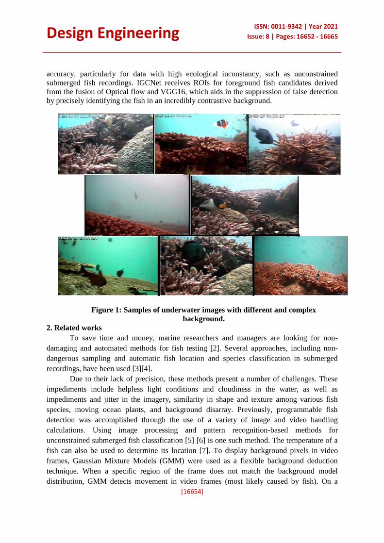
Design Engineering ISSN: 0011-9342 | Year 2021
Issue: 8 | Pages: 16652 - 16665
[16654]
accuracy, particularly for data with high ecological inconstancy, such as unconstrained
submerged fish recordings. IGCNet receives ROIs for foreground fish candidates derived
from the fusion of Optical flow and VGG16, which aids in the suppression of false detection
by precisely identifying the fish in an incredibly contrastive background.
Figure 1: Samples of underwater images with different and complex
background.
2. Related works
To save time and money, marine researchers and managers are looking for non-
damaging and automated methods for fish testing [2]. Several approaches, including non-
dangerous sampling and automatic fish location and species classification in submerged
recordings, have been used [3][4].
Due to their lack of precision, these methods present a number of challenges. These
impediments include helpless light conditions and cloudiness in the water, as well as
impediments and jitter in the imagery, similarity in shape and texture among various fish
species, moving ocean plants, and background disarray. Previously, programmable fish
detection was accomplished through the use of a variety of image and video handling
calculations. Using image processing and pattern recognition-based methods for
unconstrained submerged fish classification [5] [6] is one such method. The temperature of a
fish can also be used to determine its location [7]. To display background pixels in video
frames, Gaussian Mixture Models (GMM) were used as a flexible background deduction
technique. When a specific region of the frame does not match the background model
distribution, GMM detects movement in video frames (most likely caused by fish). On a

Design Engineering ISSN: 0011-9342 | Year 2021
Issue: 8 | Pages: 16652 - 16665
[16655]
dataset of a few submerged recordings near the Southern Taiwan district, they achieved
promising results on the fish discovery task with a normal achievement rate of 83.99 percent.
Another comparative method for displaying the covariance of the background and frontal
area (fish events) in the video outlines is to use shading and scale texture highlights. They
achieved a discovery precision of 78.01 percent in four submerged recordings with high
differentiation and illumination variations, solid background object developments, dynamic
textures, and dense background instances.
Optical flow is another movement-based method that has been used in recent years for
submerged fish identification, as well as in [9], where they proposed robot fish motion-
tracking control using optical flow as an object detecting algorithm in the controlled
aquarium environment. The use of Deep Neural Networks (DNNs) in fish identification and
species classification tasks has recently increased. Convolution Neural Network (CNN) on
Fish4Knowledge LifeCLEF 2014 and LifeCLEF 2015 fish images is also compared to other
AI strategies. An algorithm for fish recognition and grouping based on YOLO (You Only
Look Once), a CNN variant [11], has been developed. Their work included the creation of a
YOLO network based on 829 images and the identification of 93 percent of fish species
based on 100 images. [12] In another study, YOLO was used to distinguish fish cases from
each other in three different datasets, with a mean normal accuracy of 53.92 percent, while
YOLO with a parallel correlation filter was used to identify and track submerged fish
instances. Using two datasets of submerged fish, they demonstrated re-enactment results and
proposed the effectiveness of their fish tracker.
Once again, an improved deep learning framework with pre- and post-processing for
improved precision has been proposed for automatic fish identification and species
recognition on the LifeCLEF 2015 dataset [14] [15,16]. In their analysis, SSD [13] was used
to separate the foreground fish from the background fish. They obtained an F-score of 83.8
when they used CNN's ResNet-10 [15] classifier. LifeCLEF 2015 data was once again
incorporated into the GoogleNet CNN-based fish location and classification framework. They
received an F-score of 84.8 percent on the task of species classification [16].
YOLO, a deep neural network, is used to detect fast-moving fish in dynamic
environments using motion detectors in highly complex environments. They are then used to
supplement YOLO when it is unable to recognise fish due to cloudiness in the water or
because they are moving against a highly contrasted background due to their shape being
obscured by a haze.
Another advantage is that by detecting fish that are either stationary or moving
slowly, YOLO helps to suppress the fault alerts of GMMs and optical stream movement
locators [17]. For object location, a Convolutional Neural Network (CNN) called Fast R-
CNN was used, which effectively ignores background noise [18] the region recommendations
made by AlexNet as data sources, and achieves a mean normal exactness of 81.4 percent.
A CNN, on the other hand, such as AlexNet, which has three fully associated layers
and five convolutional layers, is pre-trained using a different method [19]. ImageNet's 1000-

Design Engineering ISSN: 0011-9342 | Year 2021
Issue: 8 | Pages: 16652 - 16665
[16656]
picture dataset is used for pre-training, with weights that are then applied to the
Fish4Knowledge dataset after they have been adapted. Each classification has 50 images, and
the Fish4Knowledge database has 10 classifications. Picture de-noising is used in the pre-
processing of Fish4Knowledge images, and the accuracy achieved on 1420 test images is
85.08 percent. Fish4Knowledge has so far achieved 98.64 percent detailed precision, which
was achieved by first using channels to remove the background from the first images, and
then using a CNN with a Support Vector Machine (SVM) for classification [20]. DeepFish is
the name of this approach, which consists of three standard convolution layers and three fully
connected layers. Previously, the images were usually pre-processed to remove as much noise
as possible and, in particular, to outline the shape of the fish [19, 20].
In general, previous methods included a preprocessing step to remove as much noise
from the designated image as possible and highlight the fish's outline [19, 20]. Although this
strategy can improve system performance, its methodology should be carefully tuned, as it
could result in the loss of valuable data and a negative impact on system performance. As a
result, different species may have distinct living areas that can be seen in the background.
During pre-processing, removing the species' background may result in the loss of useful
information.
To get the most out of the data and keep the results unaffected by background noise,
we need to use a robust methodology that can withstand noise and accommodate variety in
classification [21]. These techniques are well-known for preparing their network from start to
finish. We propose a deep learning-based alternative strategy for detecting and classifying
mild fish.
For example, they have used underwater camera images and recordings to discover
fish and have examined CNN using the most recent SE design to classify the data in question.
The YOLO method was used to locate the fish, and once identified, the algorithm classified
the fish to its specific species. Because the Fish4Knowledge dataset only contains exotic fish
species, we gathered another dataset of temperate fish species for this investigation. To
classify fish, we used a pre-training stage on the Fish4Knowledge dataset to prepare the
organisation to learn nonexclusive fish highlights. Following that, the learned weights were
used as the starting point for additional training on the recently gathered dataset of temperate
fish species, a process known as post-training. Transfer learning [23] is a two-process
training metric.
3. Materials and Methods
3.1. Dataset
Our proposed method has been validated using LifeCLEF 2015 (hereinafter called
LCF-15) as a benchmark. There are 93 clarified recordings in the LCF-15 dataset[24], which
includes 15 distinct species. A few video frames from LCF-15 are shown in Figure1.
Fish4Knowledge, a larger repository of underwater recordings, provided this dataset. For a
five-year period, Fish4Knowledge has gathered more than 700,000 unrestricted submerged

Design Engineering ISSN: 0011-9342 | Year 2021
Issue: 8 | Pages: 16652 - 16665
[16657]
recordings captured with fixed cameras. More than 3000 distinct fish species live in this area,
making it one of the most biodiverse places on the planet. This dataset is referred to as LCF-
15 by marine experts, and it is used to benchmark video-based fish detection and species
arrangement methods. The nine classes were chosen for this exploration. Uses species such as
AmphiprionClarkii, ChaetodonTrifascialis and ChromisChrysura as well as
HemigymnusMelapterus, MyripristisKuntee, Plectrogly-PhidodonDickii, and Zebrasoma
Scopas. There are a total of 14,765 video outlines with different fish instances that have been
commented upon. Our proposed work uses 8968 of these images. We used 70% of them for
training, i.e. 6278 images for training, and 30% for testing, i.e. 2690 images for testing.
3.2. Proposed Method
This section explains the proposed Bi-level system for underwater object detection.
Figure2 depicts the flowchart of bi-level system.Level oneidentifies the region of
interest(ROIs) for foreground fish candidates from the combined fusionof optical flow and
VGG16.Attained region of interests are fedinto the Iterative Grouped Convolution Network
(IGCNet) to categorize fish and non fish entity in second level.The Section depicts optical
flow, VGG16 and IGCNet
Figure2: Flow chart of proposed bi-level method
3.2.1 Optical Flow
Optical flow is a powerful idea that has been used to improve video classification
accuracy while requiring less computational power to perform. It has been around since 1980
Input Images
Optical Flow VGG16
Combined Fusion
Iterative Grouped
convolution
Network
Object detection (fish/
non fish)

Design Engineering ISSN: 0011-9342 | Year 2021
Issue: 8 | Pages: 16652 - 16665
[16658]
as a hand-crafted approach. Optical flow detects motion patterns generated by moving objects
in consecutive video frames and captures even minor movements, reducing missed
detections. In addition to false motion detection, it is vulnerable to false motion detection
when it comes to aquatic plants that move in the background. The optical flow features in the
underwater videos are created entirely by motion. When objects move in three dimensions,
optical flow generates a two-dimensional motion vector [24]. Optical flow can be estimated
in a variety of ways.
Optical flow is a per-pixel prediction that assumes brightness constancy, which means
it attempts to estimate how the brightness of the pixels moves across the screen over time. It
is assumed that I(x, y, t) = I(x + x, y + y, t + t). In layman's terms, this means that the pixel
characteristics at time t (i.e. rgb values) are the same as those at t, but at a different location
(denoted by x and y), where the change in location is predicted by the flow field. The
intensity vector of a pixel is evaluated by inspecting the intensity vector's successive edges.
Aside from fishes, such an investigation is prone to false movement identification when
applied to a unique background with moving oceanic plants and unexpected luminosity
variation due to unsettling influence at the water surface.
3.2.2 VGG16
The architecture diagram of VGG16 as follows
Figure3: Architecture of VGG 16
This layer's contribution is a fixed-size RGB image of the size of 224 x 224 pixels in
size. Each layer in the image is convolutional (conv. ), with a small responsive field of 3x3
(which is the smallest size for capturing the idea of left/right, up/down, and focus) for each
channel. A 1x1 convolution channel is also used in one of the arrangements; this is a straight
change of the information channels (trailed by non-linearity). After the convolution, the
spatial goal is protected by a 1-pixel padding of the convolution layer input. Five max-
pooling layers, which follow a portion of the conv. layers, complete the spatial pooling (not
all the conv. layers are trailed by max-pooling). A 2x2 pixel window is used for max-pooling
and stride 2 is used. Since VGG-16 net has a number of different pool layers, we separate the
objectness map created by each layer (pool2, pool3, etc.) In contrast to the objectness maps
created by Pool3 and Pool4, the feature map generated by Pool2 layer has a higher response
on background regions. Similarly, it makes more sense to deliver the objectness map using

Design Engineering ISSN: 0011-9342 | Year 2021
Issue: 8 | Pages: 16652 - 16665
[16659]
pool2. Pool2 has a size of 512x7x7. Instead of simply selecting the image patches relevant to
fish that have vast regions of complex background; it makes use of the overall normal
pooling in CNN to limit the number of fish. This is followed by three Fully-Connected (FC)
layers, each with 4096 channels, while the third only performs 5-way (one for each class)
instead of 1000-way. Lastly, there's a layer called soft max. As a general rule, all networks
have a similar design for their fully connected layers. The rectification (ReLU) non-linearity
has been applied to all hidden layers.
3.2.3 Image fusion
To generate a hypothetical RGB image, the blobs representing the foreground fish
candidates extracted by VGG16 and optical flow while working with input data video frames
are combined. While the third blue channel is black, the green and red channels are filled
with blobs from VGG16 and optical flow, respectively. As a result of this method, the regions
of interest (RoIs) of the foreground fish candidates appear in the resulting image. Our novel
network IGCNet is used to process the data in order to differentiate between fish species and
non-fish entities.
Table 1 displays our new Iterative Grouped Convolution Network (IGCNet) for Fish
Detection, as shown in Figure 4. Our new network will have a 46-layer architecture. It has
eight convolutional layers, two fully connected layers, softmax, and finally a classification
layer. Batch normalization is performed immediately after convolution. The ReLU is run
every time a batch is normalized. After each pooling, the data is split and aggregated twice
more. The pooling layer is used to reduce the dimensionality of data and refine convolution
output features. Convolution is used for each separation group to reduce the number of
computations and parameters to be learned..
Figure 4: Architecture of Iterative Grouped Convolution Network (IGCNet)

Design Engineering ISSN: 0011-9342 | Year 2021
Issue: 8 | Pages: 16652 - 16665
[16660]
Table 1: Description of Architecture
Conv1 5×5,64, Stride1 Group conv1 [(3,3,1),c=64)]×3
MaxPooling 3×3 Stride 2 Group conv3
Conv2 5×5,64, Stride1 Group conv2 [(5,5,1),c=64)]×3
Conv3 3×3,64, Stride1 Group conv4
Conv4 3×3,64, Stride 2 Average Pooling 3×3 Stride1
Conv5 5×5,128,Stride1 Conv7 3×3,64, Stride 3
Conv6 3×3,128, Stride1 Conv8 3×3,64, Stride 3
Batch Normalization B Followed by Relu Layer R
3.2.4 Iterative Grouped Convolution Network(IGCNet)
Grouped convolution is the process of using different sets of convolution filter groups
on the same image. This method is different from regular convolution in that the input
channels are divided up and a regular convolution is performed on each partition separately.
To reduce the computation budget and parameter cost, convolutions are performed
independently within each group. Due to its efficient compact structure and suitability for
mobile and embedded applications, group convolution has been gaining in popularity as a
way to compress and accelerate deep neural network architecture. Make a deep network with
a certain number of layers and then repeat it so that there are multiple paths for convolutions
on a single image.
When the IGCNet is trained, it is fed input images with dimensions of 224x224x3. A
64-kernel 5x5x3 convolution layer with a stride of 1 pixel is applied to the input image. Batch
Normalization is used extensively throughout the model, including on activation inputs. This
is followed by 3x3 pooling with stride 2 before the blocks are divided. Group convolution1
and group convolution2 from various blocks are now given the result of the max pooling
111x111x64. A 64-group convolution is performed with groups of 3, 3x3x1, and 5x5x1
channels. Both blocks have a standard convolutional layer after group convolution. There is a
batch normalization followed by a ReLu layer after each convolutional (either standard or
group). To obtain the feature vector, two input blocks are added element by element. A
convolutional layer8 with 3x3x64 of stride3 and a ReLu layer are both fed output from the
summation step. After a ReLU, average pooling is performed. This is followed by a splitting
operation as in the previous block. For final image representation, the split and merge results
are combined with convolution layer 8 to create a final image frame. A fully connected layer
and a softmax then receive the result. There are two types of classification layers: one for fish
and one for non-fish enitites

Design Engineering ISSN: 0011-9342 | Year 2021
Issue: 8 | Pages: 16652 - 16665
[16661]
Origina
l image
Optical
flow
image
Poolin
g
image
Fusion
image
Output
from
IGCNe
t
Figure 5: Output images from each steps involved in the bi-level system for fish
detection

Design Engineering ISSN: 0011-9342 | Year 2021
Issue: 8 | Pages: 16652 - 16665
[16662]
4. Results and Discussions
4.1. Performance Analysis
The accuracy, sensitivity, specificity, precision, recall, and F1score of the proposed
Bi-level system are used to assess its performance. The measure in table 2 shows that the
proposed algorithm outperforms the existing algorithms.
The F-score is calculated as,
F=
Where
Precision=
And
Recall=
These scores are based on the overlap of the areas of bounding boxes associated with
ground truths and detected fish. The proposed bi-level system achieved an overall detection
accuracy of 94.05 percent. Table 2 shows the proposed algorithm's performance analysis.
Table 2: Performance Analysis
Bi-Level system
Accuracy 94.05%
Sensitivity 92.19%
Specificity 99.49%
Precision 99.84%
Recall 92.19%
F1Score 95.86%
4.2. Comparison with competitive approaches
We perform fish detection using bi-level system on LCF-15 dataset and compare our
method with some recent algorithm which deals with the convolutional neural network for
object detection. The comparison result is shown in the following figure.6 and table.3.
Accuracy and performance of our bi-level system is compared with Ahsanjalal[17], Inception
V3, Resnet-50, Inception-ResNet-V2, CNN-SENet, CNN-SENet without squeeze and
Excitationnetwork. These algorithms are very recent improvement in the deep learning
environment. Our bi-level system achieves an accuracy of 94.05% improving accuracy by
11% compared to CNN-SENetwithoutSqueeze and Excitation[26],slightly better than Ahsan
Jalal (et al.,) [17].The result of the proposed bi-level method shows 94.05% of accuracy
which is higher than the other algorithms.
Table 3: Accuracy comparison of various methods
Method Accuracy
Ahsan Jalal (et al.,) [17] 91.64%
Inception-V3 88.45%
ResNet-50 90.20%
Inception-ResNet-V2 82.39%

Design Engineering ISSN: 0011-9342 | Year 2021
Issue: 8 | Pages: 16652 - 16665
[16663]
CNN-SENet[26] 87.74%
CNN-SENetwithoutSqueeze and
Excitation[26]
83.55%
Bi-level system 94.05%
Figure 6: Accuracy chart with comparison of all methods
5. Conclusion
We developed a bi-level architecture that combines optical flow, vgg16, and Iterative
grouped convolution networks to detect and localise fish instances in unconstrained
underwater videos with varying degrees of scene complexity (IGCNet). The main
contribution of this work is that it detects fish in complex backgrounds using a hybrid
approach that combines VGG16 and optical flow outputs. This fusion result is fed into the
novel IGCNet, which is used to fine-tune fish detection in the presence of non-fish entities.
This, as confirmed by the comparative study, helped to achieve cutting-edge results for the
fish detection task. In comparison to traditional computer vision and machine learning
techniques, the proposed hybrid system necessitates more computational resources but
achieves greater accuracy. Because of the advent of fast microprocessors and GPUs, deep
neural networks such as CNN can now be used for tasks that require near-real-time
processing. We believe that this research will assist fisheries scientists in adopting automatic
approaches for detecting, classifying, and tracking fish fauna in non-destructive sampling.
Furthermore, we plan to use a unified deep architecture capable of processing video
sequences in real-time in the future, thanks to rigorous optimization of our algorithm and
improved mathematical modelling. This type of setup will allow for fish detection as well as
species classification, allowing for effective fish fauna sampling.
References
[1] Jennings, S., Kaiser, M.J., 1998. The effects of fishing on marine ecosystems. In:
Advances in Marine Biology. Vol. 34. Elsevier, pp. 201–352.
[2] McLaren, B.W., Langlois, T.J., Harvey, E.S., Shortland-Jones, H., Stevens, R., 2015.
A small no take marine sanctuary provides consistent protection for small-bodied by-

Design Engineering ISSN: 0011-9342 | Year 2021
Issue: 8 | Pages: 16652 - 16665
[16664]
catch species, but not for large-bodied, high-risk species. J. Exp. Mar. Biol. Ecol. 471,
153–163.
[3] Harvey, E., Shortis, M., 1995. A system for stereo-video measurement of sub-tidal
organisms. Mar. Technol. Soc. J. 29 (4), 10–22.
[4] Shortis, M., Abdo, E.H.D., 2016. A review of underwater stereo-image measurement
for marine biology and ecology applications. In: Oceanography and Marine Biology.
CRC Press, pp. 269–304.
[5] Rova, A., Mori, G., Dill, L.M., 2007. One fish, two fish, butterfish, trumpeter:
recognizing fish in underwater video. In: MVA, pp. 404–407.
[6] Spampinato, C., Giordano, D., Di Salvo, R., Chen-Burger, Y.-H.J., Fisher, R.B.,
Nadarajan, G., 2010. Automatic fish classification for underwater species behavior
understanding. In: Proceedings of the First ACM International Workshop on Analysis
and Retrieval of Tracked Events and Motion in Imagery Streams, ACM, pp. 45–50.
[7] Hsiao, Y.-H., Chen, C.-C., Lin, S.-I., Lin, F.-P., 2014. Real-world underwater fish
recognition and identification, using sparse representation. Ecol. Inform. 23, 13–21.
[8] Palazzo, S., Murabito, F., 2014. Fish species identification in real-life underwater
images. In: Proceedings of the 3rd ACM International Workshop on Multimedia
Analysis for Ecological Data. ACM, pp. 13–18.
[9] Shin, K.J., 2016. Robot fish tracking control using an optical flow object-detecting
algorithm. IEIE Trans. Smart Process. Comput. 5 (6), 375–382.
[10] Salman, A., Jalal, A., Shafait, F., Mian, A., Shortis, M., Seager, J., Harvey, E., 2016.
Fish species classification in unconstrained underwater environments based on deep
learning. Limnol. Oceanogr. Methods 14 (9), 570–585.
[11] Sung, M., Yu, S.-C., Girdhar, Y., 2017. Vision based real-time fish detection using
convolutional neural network. In: OCEANS 2017-Aberdeen. IEEE, pp. 1–6.
[12] Xu, W., Matzner, S., 2018. Underwater fish detection using deep learning for water
power applications. In: arXiv preprint arXiv:1811.01494.
[13] Liu, W., Anguelov, D., Erhan, D., Szegedy, C., Reed, S., Fu, C.-Y., Berg, A.C.,
2016. Ssd: Single shot multibox detector. In: European Conference on Computer
Vision. Springer, pp. 21–37.
[14] Zhuang, P., Xing, L., Liu, Y., Guo, S., Qiao, Y., 2017. Marine Animal Detection and
Recognition with Advanced Deep Learning Models, Working Notes of CLEF 2017.
[15] Hariharan, B., Girshick, R.B., 2017. Low-shot visual recognition by shrinking and
hallucinating features. In: ICCV, pp. 3037–3046.
[16] Choi, S., 2015. Fish identification in underwater video with deep convolutional
neural network: Snumedinfo at lifeclef fish task 2015. In: CLEF (Working Notes).
[17] AhsanJalala , Ahmad Salmana , AjmalMianb , Mark Shortisc , Faisal Shafaita 2020
.Fish detection and species classification in underwater environments using deep
learning with temporal information Ecological Informatics 57 (2020) 101088

Design Engineering ISSN: 0011-9342 | Year 2021
Issue: 8 | Pages: 16652 - 16665
[16665]
[18] X. Li, M. Shang, H. Qin, L. Chen, “Fast accurate fish detection and recognition of
underwater images with fast r-cnn “ in OCEANS’15 MTS/IEEE Washington (IEEE,
2015), pp. 1–5
[19] L. Jin, H. Liang, “Deep learning for underwater image recognition in small sample
size situations.” in OCEANS 2017-Aberdeen (IEEE, 2017), pp. 1–4.
[20] H. Qin, X. Li, J. Liang, Y. Peng, C. Zhang,” DeepFish: Accurate underwater live fish
recognition with a deep architecture”, Neurocomputing 187, 49 (2016)
[21] M. Pedersen, J.B. Haurum, R. Gade, T.B. Moeslund, “Detection of Marine Animals
in a New Underwater Dataset with Varying Visibility” in CVPR Workshops (2019)
[22] J. Yosinski, J. Clune, Y. Bengio, H. Lipson, CoRR “How transferable are features in
deep neural networks?” abs/1411.1792 (2014)
[23] Warren, D.H., Strelow, E.R., 2013. Electronic Spatial Sensing for the Blind:
Contributions from Perception, Rehabilitation, and Computer Vision. Vol. 99
Springer Science & Business Media.
[24] LifeClef2015 dataset link: https://www.imageclef.org/lifeclef/2015/fish
[25] Knausgård, K.M., Wiklund, A., Sørdalen, T.K. et al. Temperate fish detection and
classification: a deep learning based
approach. ApplIntell (2021).https://doi.org/10.1007/s10489-020-02154-9
n
View publication statsView publication stats
www.jespublication.com Page No:1029
Vol 11, Issue 6,June/ 2020
ISSN NO: 0377-9254
IMPLEMENTATION OF DEEP LEARNING TECHNIQUES TO
ADDRESS CORAL REEF DISEASES M. H. Ibrahim1 and M. Mohamed Sathik2
1Research Scholar, Sadakathullah Appa College, Tirunelveli, Tamilnadu, India
2Principal and Research Supervisor, Sadakathullah Appa College, Tirunelveli, Tamilnadu, India
Abstract— Coral reefs is an important,
unavoidable attribute of the marine ecosystem.
It plays a major role in keeping the ecosystem
balanced. Coral reefs produces nutrition and
proteins to the fishes like tuna, dolphin and
other pelagic species. But, due to industrial
pollution, human-related activities, climate
change, bleaching, the total amount of the coral
reefs has drastically reduced. According to the
report of Global Coral Reef Monitoring
Network (GCRMN) around 19% of coral reefs
in the world has lost in last 30years and it is
expected to lose another 17% by 2030. It has
also predicted that, in 2050, all the coral reefs in
the world will be in danger. To address this
alarming issue, this research work proposes a
deep convolution neural network machine
learning technique to identify the infected or
diseased corals from videos. Here, two datasets
are used. One is used to train the neural
network to predict the type of the coral reef
downloaded from Mendeley open source archive
and second dataset is used to predict whether
the particular coral is affected from white
plague disease or not. The second video dataset
is downloaded from official BBC Earth
YouTube web channels in HD 720 pixel. These
data are given as input to the Deep Convolution
Neural Network (DCNN) to perform image
classification. The proposed system
automatically predicts the diseases in the coral
reefs and helps in improving the coral
ecosystem.
Keywords— Deep learning; Coral reefs;
Disease prediction; Coral ecosystem; neural
networks.
1. INTRODUCTION
Coral reefs are living, colorful, multi-faceted
structure, which are the part of marine ecosystem.
Coral reefs are formed by calcium carbonates and
are mostly present near equator of the world. It
lives in warm water and maintains a temperature
between 20 to 28 degree Celsius It creates a
colony-like structure to shelter species like fishes,
crabs, sea stars, shrimps and algaes [1]. It is
estimated that around one lakh different species are
living under the coral reefs. It also produces
nutrition and proteins to the species that live on the
ocean. Moreover, it also helps human being by
providing coral foods, shorelines protection and
medicines. On the basis of recent report from
National Oceanic and Atmospheric Administration,
the annual economy earning of coral reef mining is
about 30 billion US dollars.
Coral reefs has most variety of all marine
ecosystem. There are more than 2500 species of
coral reefs in the world. Around 40 percent coral
are hard in nature. It will not have any motion or
movements in the ocean. They will look like a hard
rock. On the other hand, remaining 60 percent of
corals are soft in nature [2]. It will have a skeletons
that are flexible to make motions on the water.
Though, it gives several advantages to the
ecosystem and human being, coral reefs are now in
great danger due to industry pollution, overfishing,
destructive fishing and climate change. In some
places on earth, the coral reefs are entirely
destroyed and in many places coral reefs are in
endangered situation.
Diseases spreading on the coral reefs are also an
important reason for the degradation. Diseases like
vibrio, white syndrome, white band, and rapid
wasting disease. In here, the white syndrome and
white band are the wide spread disease in the entire
world. These diseases forms a white colored foam
in the surfaces of the coral reefs. It also exhibits a
pronounced division between the remaining coral
tissue and the exposed coral skeleton. White layer
diseases such as white band and syndrome in the
coral reefs can be categorized into Type I and Type
II diseases. In here, Type I, diseases doesn’t show
any bleaching on the upper layer of the coral reefs.
But it changes the color slightly. Type II coral reef
diseases bleaches the surface completely[3].
In this research work, we intended to create a
framework to identify the corals types and its

www.jespublication.com Page No:1030
Vol 11, Issue 6,June/ 2020
ISSN NO: 0377-9254
disease automatically by performing deep learning
techniques on the coral reef video dataset. Here, we
have used Deep Convolution Neural Network
(DCNN) to identify the data coral type and its
diseases.
Deep Convolution Neural Network (DCNN) is a
type of neural network, which perform both
forward and backward propagation to gather
information, identify the relationship and detects
patterns between the data. CNN has a fully
connected multi-layer neuron structure, in which
each neurons in a layer is connected with all the
neurons in the adjacent layers. It uses linear
convolution operation at least in any one of the
layer. Convolution Neural Network (CNN) takes
input as image and assign importance to various
aspects in the image and classifies it [4].
In this research work, a coral reef image dataset
(downloaded from Mendeley open archive) is
given as input to train and a video dataset from
BBC Earth is used to test the proposed DCNN
framework.
This research work is organized as, Section 2,
describes the related works that are carried out on
predicting the type and the disease spread in the
coral reefs. Section 3, explains the proposed
implementation and framework of proposed Deep
Convolution Neural Network used. Section 4,
evaluates the performance of the proposed
approach and Section 5 concludes and discusses
about the future work.
2. RELATED WORKS
In early days, information related to coral reefs are
collected from underwater visual censuses (UVC)
by scuba divers. The accuracy of the collected
information is highly depends on the depth,
duration and the experience of the scuba divers.
Identifying the type, growth, disease in the coral
reefs were difficult. But, after the rapid
advancement in robotic technology and under
water cameras, information related to the coral
reefs and marine ecosystem are captured using
video supported under water rovers and automatic
motion capturing devices [5].
However, collecting and observing information
about the coral reefs need an oceanic research
specialists. Moreover, observing information from
a long video is a time consuming and expensive
operation. So there is an immediate need to create a
framework to perform automatic coral reef
classification and disease prediction to improve the
coral ecosystem. Images captured through
underwater rovers is shown in Fig. 1 and the
example image of jelly fish rover is shown in Fig.2.
In order to achieve such an automated image
classification method, deep learning techniques are
used.
Fig. 1 Image captured through underwater
video rovers Fig. 2 Image of jelly fish rover
One of the important subset of deep learning
technique is Neural Networks (NN). It has been
used in several applications text classification,
paraphrase detection, facial recognition, speech
recognition and much more. In recent time, it has
been used in oceans to keep track of ocean wave
power, endangered fishes and temperature monitor.
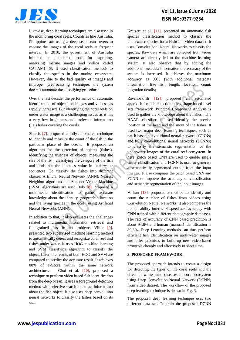
www.jespublication.com Page No:1031
Vol 11, Issue 6,June/ 2020
ISSN NO: 0377-9254
Likewise, deep learning techniques are also used in
the monitoring coral reefs. Countries like Australia,
Philippines are using a deep sea ocean rovers to
capture the images of the coral reefs at frequent
interval. In 2010, the government of Australia
initiated an automated tools for capturing,
analyzing marine images and videos called
CATAMI [6]. It used classification methods to
classify the species in the marine ecosystem.
However, due to the bad quality of images and
improper preprocessing technique, the system
doesn’t automate the classifying procedure.
Over the last decade, the performance of automatic
identification of objects on images and videos has
rapidly increased. But identifying the coral reefs on
under water image is a challenging issues as it has
a very low brightness and irrelevant information
(i.e.) fishes covering the corals.
Shortis [7], proposed a fully automated technique
to identify and measure the count of the fish in the
particular place of the ocean. It proposed an
algorithm for the detection of objects (fishes),
identifying the trueness of objects, measuring the
size of the fish, classifying the category of the fish
and finds out the biomass value in underwater
sequences. To classify the fishes into different
classes, Artificial Neural Network (ANN), Nearest
Neighbor algorithm and Support Vector Machine
(SVM) algorithms are used. Joly [8], proposed a
multimedia identification to gather accurate
knowledge about the identity, geographic location
and the living species in the ocean using Artificial
Neural Networks (ANN).
In addition to that, it also evaluates the challenges
related to multimedia information retrieval and
fine-grained classification problems. Villon [9],
presented two supervised machine learning method
to automatically detect and recognize coral reef and
fishes under water. It uses HOG machine learning
and SVM classifying algorithm to classify the
object. Later, the results of both HOG and SVM are
compared to predict the accurate result. It achieves
88% of F-Score within the same network
architecture. Choi et al. [10], proposed a
technique to perform video based fish identification
from the deep ocean. It uses a foreground detection
method with selective search to extract information
about the fish object. It also uses deep convolution
neural networks to classify the fishes based on its
size.
Kratzert et al. [11], presented an automatic fish
species classification method to classify the
underwater species for a FishCam video dataset. It
uses Convolutional Neural Networks to classify the
species. Raw data which are collected from video
camera are directly fed to the machine learning
system. It also observe that by adding the
additional metadata information the accuracy of the
system is increased. It achieves the maximum
accuracy as 93% (with additional metadata
information like fish length, location, count,
migration details)
Ravanbakhsh [12], proposed an automated
approach for fish detection using shape based level
sets framework. Principal Component Analysis is
used to gather the knowledge about the fishes. The
HAAR classifier is used identify the precise
location of the head and the snout of the fishes. It
used two major deep learning techniques, such as
patch based convolutional neural networks (CNNs)
and fully convolutional neural networks (FCNNs)
to classify the semantic segmentation of the
underwater images of the coral reef ecosystem. In
here, patch based CNN are used to enable single
entity classification and FCNN is used to generate
a semantically segmented output from the input
images. It also compares the patch based CNN and
FCNN to improve the accuracy of classification
and semantic segmentation of the input images.
Villion [13], proposed a method to identify and
count the number of fishes from videos using
Convolution Neural Networks. It also compares the
human ability interns of speed and accuracy with
CNN trained with different photographic databases.
The rate of accuracy of CNN based prediction is
about 94.6% and human (manual) identification is
89.3%. Deep Learning methods can thus perform
efficient fish identification on underwater images
and offer promises to build-up new video-based
protocols cheaply and effectively in short time.
3. PROPOSED FRAMEWORK
The proposed approach intends to create a design
for detecting the types of the coral reefs and the
effect of white band diseases in coral ecosystem
using Deep Convolution Neural Network (DCNN)
from video dataset. The workflow of the proposed
deep learning technique is shown in Fig. 3.
The proposed deep learning technique uses two
different data set. To train the proposed DCNN

www.jespublication.com Page No:1032
Vol 11, Issue 6,June/ 2020
ISSN NO: 0377-9254
model we have used, an open-source image dataset
which is collected from Mendeley Open Archives
from Universitat de Girona - Campus de Montilivi.
The dataset consist of a huge amount of images and
information about the different coral reef species.
We have also used a second dataset to test the
performance of the proposed method. The second
dataset is a 10 hours video download from official
BBC Earth YouTube web channel in HD 1080p.
To train the Deep Convolution Neural Network
(DCNN), the chosen image dataset has to undergo
a preprocessing method to purify the error data
from the dataset. Raw image dataset might have
low quality as the images are captured under water.
The preprocessing technique will improve the
quality and accuracy of the image dataset, which
will impacted on the overall accuracy of the
proposed deep learning technique.
3.1 Data Pre-processing of test dataset
Pre-processing is an important feature of deep
learning technique which process the raw data and
converts in a knowledgeable format which are later
given as the input to the Deep Convolution Neural
Network(DCNN). Under water image will have
noises like,
Fig. 3. Workflow to identify the type and condition of white band diseases affected in coral reefs using
DCNN
Gaussian noise, Salt and pepper noise, shot noise,
quantization noise, film grain noise, low light
noise, anisotropic and periodic noise.
To remove these noise and improve the quality of
image two important method are used to preprocess
the underwater images. They are image restoration
and image enhancement.
In image restoration, an arithmetic mean filter is
used to de-noising the underwater images and then
an iterative deconvolution method is used to filter
out the images. Information like attenuation,
coefficients, scattering and depth estimation of the
object (fishes) are fed as the input along with the
image.
Later in image enhancement preprocessing method,
disturbance or noises in the images are corrected
sequentially. Initially, it removes the over applied
effects using the homomorphic filters on the image
to improve the quality of the image. It also used to
remove the defects of non-uniformity of
illumination and improves the contrasts. Fig. 4
represents the preprocessed image and raw image.
Later the preprocessed data are fed to a specified
Uniform Ratio Aspect (URF) module to crop the
images into a square shaper. Because most of the
neural networks performs on the square shaped
image. For cropping the images, the middle part of
the image is chosen. The preprocessing algorithm
takes middle part of the image and draws multiple
square shaped crops and find the best fit.
Fig. 4 (a) Raw extracted image

www.jespublication.com Page No:1033
Vol 11, Issue 6,June/ 2020
ISSN NO: 0377-9254
Fig. 4 (b) Preprocessed image
3.2 Feature selection
Feature selection is also an important and
unavoidable task in Deep learning. It aims to find a
small number of features that describes the image
dataset
Fig. 5 Relief feature selection algorithm of image dataset
better than the original set of features. This can be
achieved by removing irrelevant and redundant
features according to importance criterion in
feature selection. To remove the irrelevant data
from the raw dataset, relief feature selection
algorithm is used. The images on the dataset is
consider as instances and the object belonging to a
known classes are called as feature of the dataset.
Let us consider, ‘n’ instances and ‘p’ features in a
dataset. Each features in the dataset is scaled
between the value 0 and 1. Now, take the feature
vector X from a random instance and another
feature vector X from its nearest instance using
Euclidean distance. This operation is performed in
an iterative manner. The closest instance is
considered near-hit and the longest distanced
instance is considered as near-miss. At each
iteration, the weight of the vector is updated.
Weight of the feature vector can be calculated
from,
Weight (i) = Weight (i-1) – (Xi - near hiti) 2 + (Xi -
near missi) 2
After find out the weight for each feature vector,
the median value is set as threshold for feature
selection. Fig. 5, shows the procedure of feature
extraction.
3.3. Deep Convolution Neural Networks
Deep Convolution Neural Network is a subset of
deep neural networks, which is used to analyze,
classify the image and video dataset. It is also
called as Shift Invariant Neural Network (SIANN).
It has been used in face recognition, image
classification, recommendation system, medical
image analysis.
Fig. 6 Structure of the Neural Networks
Every layer in neural networks will have several
neurons in each layer. CNN system takes input as
images, process it and classifies the input dataset
into classes based on the features of the image. In
here, the result produced by the feature extraction
algorithm is processed and separates the images
based on the type of the corals reefs. Each input in
the dataset will undergo through a series of
convolutions layers, where each layer will have a
kernel filters, pooling and softmax function to
classify the image with probabilistic value of 0 to
1. Convolution uses the relationship between the
pixels and small-square as input to learn the

www.jespublication.com Page No:1034
Vol 11, Issue 6,June/ 2020
ISSN NO: 0377-9254
features on the image. Filters in each layer perform
task like edge detection, blur handling, sharpening
the image.
Meanwhile, the classification based on the
convolution filters alone can’t give a perfect result.
To improve the prediction result in the convolution
layer, padding is also used. For example, if the size
of the filter used is 3*3 matrix and the input image
size is 8*8, then the filter can’t efficiently process
the input data. In such scenario, padding can be
used.
The system artificially adds, n*n zero matrix values
to the image to equals the inputs data size. The
added pixel will have the zero value and doesn’t
affect the convolution neural network in any
means. The process of kernal filter and padding
are continuously performed in an iteration manner
and allows the input data to propagate forward and
backward and makes the system to learn about the
input image.
Once after the DCNN is learned about the coral
reefs and its type. The second dataset (i.e.) test
dataset (video files) is given as input the DCNN.
Later, the video dataset is extracted in scale of 2
images per second (120 image per minute) of a
total 10hours videos. These frame extraction is
performed using video capturing function in
OpenCV. These test dataset is fed to the CNN
again to check the accuracy of the proposed DCNN
based automatic prediction technique.
Once after finding out the type of the coral reefs, an
separate support vector machine (SVM) base
machine learning technique is used to classify
whether the coral reef has affected from white band
disease or not.
4. EXPERIMENTS
The proposed Deep Convolution Neural Network
experiment to identify the type of the coral reef and
to derive the information about the white band
disease on the surface of the coral reefs are carried
out on an open source software called, Tensor Flow
software. The dataset used for the implementation
is taken from Mendeley Imaging Archive site. The
downloaded data had several information related to
the type of the coral reef. The total number of the
coral reef images present in the first dataset is
around 1,512, in which 80% of images (i.e.) 1,259
images is chosen as training images and remaining
20% of images are used as the testing dataset. The
first dataset is used to train the neural network to
classify the type of the coral reefs. The second
dataset used to train the neural networks is a video
dataset, which is downloaded from the BBC Earth
YouTube Channel consist of a total run time of
3.12 hours of oceanography and underwater videos
shot beneath the sea. Total of 22,462 images are
derived from the video (i.e.) two images per
second. Due to the limitation of processing
capacity in the computer system, a total of 3000
images were chosen from 22,462 image derived
from the video. Later in these 3,000 videos, 80%
are used as training data set and 20% are used as
test data. The second dataset is used to identify
whether the coral reefs is infected by the white
band diseases are not.
The implementations were carried out on an i7
Intel processor system with 8GB with the
computing power and 1TB storage space. The
overall performance of the proposed DCNN is
measured using three major evaluation aspects of
the ML algorithm such as accuracy of the results,
precision and recall.
To measure the accuracy of the proposed DCNN
method, four major factors are considered, such as
true positive (TP), true negative (TN), false
negative (FN) and false positive (FP). The true
positive is the case, in which the type of the coral
reef is identified correctly. The true negative is the
case, where the coral relief belong to a particular
type and DCNN fails to find it. The false positive is
the case where the coral reef is not belong to a
particular type and DCNN results the same. False
negative is the case, where the coral reed doesn’t
belong to a type, but DCNN wrongly predicts that
the coral reef belong to particular type. The
formula to measure the accuracy of the proposed
system is,
The measured accuracy of the proposed model
DCNN model is 92.1%. In total of 253 test set
images, the DCNN system correctly predicted the
type of 233 images. However, accuracy of SVM
algorithm to predict the same is 80.6%, (i.e.) 203
images. The accuracy of the proposed DCNN
method is measured and compared with other
existing methods. Likewise, the sensitivity is also
measured. Sensitivity is a measure of the
proportion of actual positive cases that got
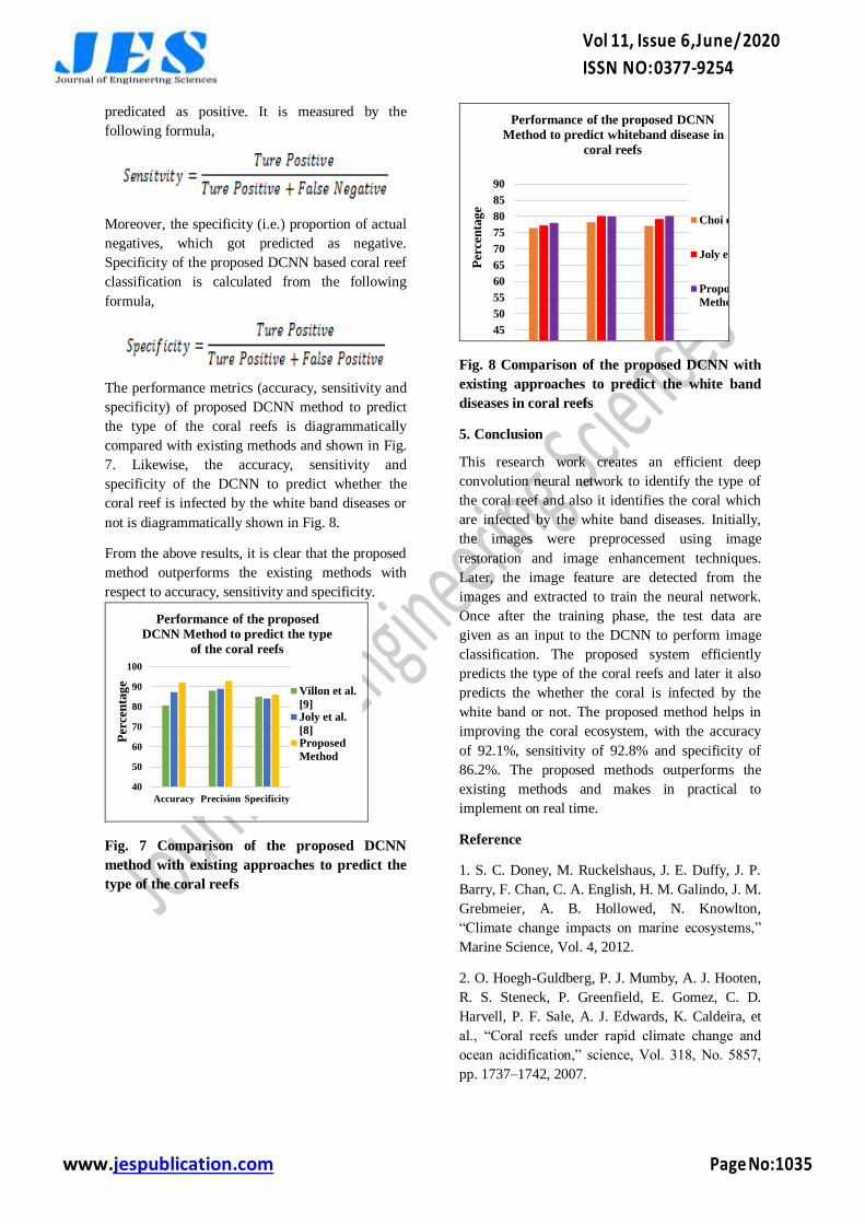
www.jespublication.com Page No:1035
Vol 11, Issue 6,June/ 2020
ISSN NO: 0377-9254
predicated as positive. It is measured by the
following formula,
Moreover, the specificity (i.e.) proportion of actual
negatives, which got predicted as negative.
Specificity of the proposed DCNN based coral reef
classification is calculated from the following
formula,
The performance metrics (accuracy, sensitivity and
specificity) of proposed DCNN method to predict
the type of the coral reefs is diagrammatically
compared with existing methods and shown in Fig.
7. Likewise, the accuracy, sensitivity and
specificity of the DCNN to predict whether the
coral reef is infected by the white band diseases or
not is diagrammatically shown in Fig. 8.
From the above results, it is clear that the proposed
method outperforms the existing methods with
respect to accuracy, sensitivity and specificity.
40
50
60
70
80
90
100
Accuracy Precision Specificity
Per
cen
tag
e
Performance of the proposed
DCNN Method to predict the type
of the coral reefs
Villon et al.
[9]Joly et al.
[8]Proposed
Method
Fig. 7 Comparison of the proposed DCNN
method with existing approaches to predict the
type of the coral reefs
40
45
50
55
60
65
70
75
80
85
90
Per
cen
tag
e
Performance of the proposed DCNN
Method to predict whiteband disease in
coral reefs
Choi et al. [10]
Joly et al. [8]
Proposed
Method
Fig. 8 Comparison of the proposed DCNN with
existing approaches to predict the white band
diseases in coral reefs
5. Conclusion
This research work creates an efficient deep
convolution neural network to identify the type of
the coral reef and also it identifies the coral which
are infected by the white band diseases. Initially,
the images were preprocessed using image
restoration and image enhancement techniques.
Later, the image feature are detected from the
images and extracted to train the neural network.
Once after the training phase, the test data are
given as an input to the DCNN to perform image
classification. The proposed system efficiently
predicts the type of the coral reefs and later it also
predicts the whether the coral is infected by the
white band or not. The proposed method helps in
improving the coral ecosystem, with the accuracy
of 92.1%, sensitivity of 92.8% and specificity of
86.2%. The proposed methods outperforms the
existing methods and makes in practical to
implement on real time.
Reference
1. S. C. Doney, M. Ruckelshaus, J. E. Duffy, J. P.
Barry, F. Chan, C. A. English, H. M. Galindo, J. M.
Grebmeier, A. B. Hollowed, N. Knowlton,
“Climate change impacts on marine ecosystems,”
Marine Science, Vol. 4, 2012.
2. O. Hoegh-Guldberg, P. J. Mumby, A. J. Hooten,
R. S. Steneck, P. Greenfield, E. Gomez, C. D.
Harvell, P. F. Sale, A. J. Edwards, K. Caldeira, et
al., “Coral reefs under rapid climate change and
ocean acidification,” science, Vol. 318, No. 5857,
pp. 1737–1742, 2007.
www.jespublication.com Page No:1036
Vol 11, Issue 6,June/ 2020
ISSN NO: 0377-9254
3. T. C. Bridge, R. Ferrari, M. Bryson, R. Hovey,
W. F. Figueira, S. B. Williams, O. Pizarro, A. R.
Harborne, and M. Byrne, “Variable responses of
benthic communities to anomalously warm sea
temperatures on a high-latitude coral reef,” Plos
One Journal, Vol. 9, No. 11, pp. 1-10, 2014. DOI:
10.1371/journal.pone.0113079.
4. Aloysius, N., & Geetha, M. “A review on deep
convolutional neural networks” International
Conference on Communication and Signal
Processing (ICCSP), 2017
DOI:10.1109/iccsp.2017.8286426.
5. Boström-Einarsson L, Babcock RC, Bayraktarov
E, Ceccarelli D, Cook N, Ferse SCA, et al. (2020)
“Coral restoration – A systematic review of current
methods, successes, failures and future directions”
PLoS ONE 15(1), 2020. DOI:
10.1371/journal.pone.0226631
6. Althaus F, Hill N, Ferrari R, Edwards L,
Przeslawski R, Schönberg CHL, A Standardised
Vocabulary for Identifying Benthic Biota and
Substrata from Underwater Imagery: The CATAMI
Classification Scheme. PLoS ONE 10(10), 2015.
DOI: 10.1371/journal.pone.0141039.
7. M. Shortis, B. Ghanem, P.F. Culverhouse, D.
Edgington, D. Cline, M. Ravanbakhsh, J. Seager,
E.S. Harvey, Fish identification from videos
captured in uncontrolled underwater environments,
ICES J. Marine Sci.: J. Conseil (2016) 106
8. Joly, A., Goëau, H., Glotin, H., Spampinato, C.,
Bonnet, P., Vellinga, W.-P, Müller, H. (2015).
LifeCLEF 2015: Multimedia Life Species
Identification Challenges. Experimental IR Meets
Multilinguality, Multimodality, and Interaction,
462–483. DOI:10.1007/978-3-319-24027-5_46.
9. Villon, S., Chaumont, M., Subsol, G., Villéger,
S., Claverie, T., & Mouillot, D. (2016). Coral reef
fish detection and recognition in underwater videos
by supervised machine learning: Comparison
between deep learning and HOG+ VM methods,
Advanced Concepts for Intelligent Vision Systems.
ACIVS 2016. Lecture Notes in Computer Science,
Vol. 10016.
10. Sungbin Choi, “Fish Identification in
Underwater Video with Deep Convolutional Neural
Network: SNUMedinfo at LifeCLEF Fish task
2015. CLEF (Working Notes) 2015
11. Kratzert, F., & Mader, H. (2017, April).
Advances of FishNet towards a fully automatic
monitoring system for fish migration. In EGU
General Assembly Conference Abstracts (Vol. 19,
p. 7932).
12. Mehdi Ravanbakhsh, Faisal Shafait, Euan S.
Harvey, ―Automated Fish Detection In
Underwater Images Using Shape-Based Level
Sets‖, 2015.
13. Villon, S., Mouillot, D., Chaumont, M.,
Darling, E. S., Subsol, G., Claverie, T., and
Ville´ger, S. 2018. A deep learning method for
accurate and fast identification of coral reef fishes
in underwater images. Ecological Informatics, 48:
238–244