AUTOMATED CONTOUR DETECTION

IN ECHOCARDIOGRAPHIC IMAGES

Hans Bosch

2

ISBN-10: 90-810712-1-1 ISBN-13: 978-90-810712-1-5 Automated contour detection in echocardiographic images. Johannes Gijsbertus Bosch Proefschrift Universiteit Leiden. Met samenvatting in het Nederlands. © 2006 by J.G. Bosch, except for the following chapters: Chapter 1: © 2002 W.B. Saunders Company Chapter 2: © 1995 The American Society of Echocardiography Chapter 4,5: © 2002 The Institute of Electrical and Electronic Engineers Inc. Chapter 6: © 2003 The Society of Photo-Optical Instrumentation Engineers Cover photo of El Capitan: © Nick Strobel (www.astronomynotes.com) No part of this thesis may be reproduced in any form by print, photocopy, in digital format or by any other means without prior written permission of the author. Keywords: echocardiography, automated border detection, heart, left ventricle, ultrasound Printed by Universal Press, Veenendaal. Cover design: Hans Bosch and Universal Press.

AUTOMATED CONTOUR DETECTION

IN ECHOCARDIOGRAPHIC IMAGES

Automatische contourdetectie in echocardiografische beelden

Proefschrift

ter verkrijging van

de graad van Doctor aan de Universiteit Leiden,

op gezag van de Rector Magnificus Dr. D.D. Breimer,

hoogleraar in de faculteit der Wiskunde en

Natuurwetenschappen en die der Geneeskunde,

volgens besluit van het College voor Promoties

te verdedigen op maandag 12 juni 2006

klokke 16.15 uur

door

Johannes Gijsbertus Bosch

Geboren te Berlicum

in 1960

4

PROMOTIECOMMISSIE Promotores: Prof. dr. ir. J.H.C. Reiber Prof. dr. M. Sonka (University of Iowa, Iowa City, IA, USA) Referent: Prof. dr. ir. N. Bom (Erasmus Universiteit Rotterdam) Overige leden: Prof. dr. E.E. van der Wall Prof. dr. A.F.W. van der Steen (Erasmus Universiteit Rotterdam) Dr. J. Dijkstra The studies described in this thesis were primarily performed at the Division of Image Processing (LKEB), Department of Radiology, Leiden University Medical Center, Leiden, the Netherlands. The research described in chapters 2-5 was financially supported by the Dutch Technology Foundation STW (grants LGN 92.1706 and LGN66.4349). Financial support for the studies described in chapter 5 and 6 was provided by the BTS-program of the Ministry of Economic Affairs (Ministerie van Economische Zaken), the Netherlands (grant BTS 00123) Financial support for the studies described in chapter 3 was partly provided by Medis medical imaging systems bv, Leiden, the Netherlands. Financial support for the publication of this thesis by the following organizations is gratefully acknowledged: Stichting Beeldverwerking Leiden Medis medical imaging systems bv Bio-Imaging Technologies, B.V.

5

To my parents - trust

To Rietje and Jan - hope

To Simone, Tom and Bram - love

6

7

Contents

Preface...................................................................................................................9 1. Two-dimensional echocardiographic digital image processing ..........................11

and approaches to endocardial edge detection. (in: The practice of clinical echocardiography. Second edition, 2002.

Otto CM (ed.). Orlando, FL, W.B. Saunders: 141-158) 2. Evaluation of a semiautomatic contour detection approach in ............................41

sequences of short-axis two-dimensional echocardiographic images. (J Am Soc Echocardiogr 8 (1995): 810-21) 3. Automated contour detection in echocardiographic image sequences ................61

using dynamic programming, pattern matching and spatiotemporal geometric models.

4. Automatic segmentation of echocardiographic sequences ..................................87

by active appearance motion models. (IEEE Trans Med Imaging 21 (2002): 1374 -1383) 5. 3-D Active Appearance Models: .......................................................................109

segmentation of cardiac MR and ultrasound images. (IEEE Trans Med Imaging 21 (2002): 1167-1178) 6. Automated classification of wall motion abnormalities by ...............................133

principal component analysis of endocardial shape motion patterns in echocardiograms.

(Proceedings SPIE Vol. 5032, Medical Imaging 2003: Image Processing: 38-49)

7. Clinical and research applications of developments in automated ....................153

echocardiographic contour detection. Conclusions .......................................................................................................197 Summary ...........................................................................................................199 Samenvatting.....................................................................................................205 Acknowledgements ...........................................................................................211

Contents

8

About the cover .................................................................................................215 Full color supplement........................................................................................217 Publications .......................................................................................................221 Curriculum Vitae...............................................................................................227

9

Hier zit ik, in elke hand een manchetknoop,

aan elke manchetknoop een halve meteoriet. Samen een hele.

Maar geen enkel bewijs voor de hypothese die ik bewijzen moest.

Slotzin van Nooit meer slapen

Willem Frederik Hermans

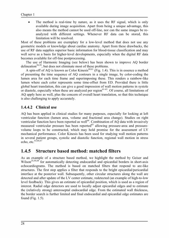
Preface

Echocardiography or cardiac ultrasound is the most widely applied imaging technique for the evaluation of anatomy and function of the heart. It is generally non-invasive and no ionizing radiation is involved. There are few contra-indications and there is no evidence of negative effects for patients or medical staff. Equipment is relatively cheap, versatile, flexible in use and mobile.

At the same time, echocardiography is not an easy imaging modality for interpretation or analysis - images appear noisy and are hampered by artifacts such as false echoes, dropouts, shadowing, etc.

The proper operation of a modern echocardiograph is not a simple task at all - the complexity comes close to that of a small airplane's cockpit and not many users are familiar with the complete functionality and all its possibilities. Also, the physical properties of ultrasound sometimes limit its applicability, e.g. in obese patients or in case of poor acoustical windows.

From the medical viewpoint, interpretation of the images requires a high level of anatomical insight, knowledge of the physics of ultrasound and familiarization to the common appearance of anatomical structures and typical artifacts.

From the image processing point of view, images are anisotropic, extremely nonlinear in any sense, hardly reproducible and there is no simple relation between physical tissue properties and image intensities.

It is very important to extract quantitative information from such images, for obtaining objective diagnoses, verifying the effect of interventions, etc. Common measurements include the anatomical dimensions such as the length of long and short axis of the left ventricle, volumes at end-diastole and end-systole and ejection fraction, or more complex measures such as sphericity, regional wall motion patterns, or wall thickness curves.

It is possible to calculate such measures from manually drawn contours or markers, but this suffers from large inter- and intra-observer variabilities and is often impractical, since many images need to be analyzed consistently. Therefore, there is a great need for automated image analysis tools.

Preface

10

This thesis covers the computerized, automated analysis and quantification of important structures in echocardiographic images. The main topics of our research were the automated detection and tracking of the endocardial border of the left heart chamber, and the subsequent analysis of the endocardial wall motion. The setup of the thesis is as follows. Chapter 1 provides a general introduction into digital image processing as applied to echocardiographic images and sketches the most commonly applied approaches for border detection in echocardiography, including the ones elaborated upon in our research. Chapter 2 is dedicated to the most classical border detection problem in echocardiography, detection of the endocardium in short-axis cross-sectional images, and our solution for that. Chapter 3 covers a more elaborate approach for endocardial border tracking in cross-sectional images acquired along the major axis of the left ventricle (e.g. apical four- and two-chamber images, parasternal long-axis). Chapter 4 is devoted to the application of a new class of border detection techniques, the Active Appearance Models. In chapter 5, an extension of these models to a three-dimensional space is described, which makes them highly attractive for time sequences of two-dimensional images as well. Chapter 6 describes a novel approach for automatic classification of wall motion abnormalities from detected borders, which is directly derived from the statistical shape modeling described in the previous chapters. Chapter 7 lists the clinical applications of the research described in the previous chapters, as well as some important spin-offs from our work that would otherwise not be covered in this thesis. In this way, we hope to supply a more complete and unifying image of the total research endeavors. Finally, some conclusions are presented.

11

Chapter 1

Two-dimensional echocardiographic

digital image processing and approaches to endocardial edge detection.

A description of goals and pitfalls.

Hans G. Bosch and Johan H.C. Reiber

Division of Image Processing, Department of Radiology, Leiden University Medical Center, Leiden, The Netherlands.

Published as Chapter 7 of The practice of clinical echocardiography, Second edition, 2002. Catherine M. Otto (ed). Philadelphia, PA: W.B. Saunders, p.141-158.

ISBN 0-7216-9204-4

Chapter 1

12

Chapter 1

13

1.1 Introduction Digital image processing techniques nowadays can be found in any ultrasound machine or off-line analysis system. Moreover, ultrasound machines have evolved from mainly analog, video-type technology into fully digital, computer-like systems. Digital image storage and digital processing of echocardiographic images, both for image enhancement and analysis, is widely practiced. Some forms of automated image analysis and automated border detection (ABD) techniques (also known as edge detection, border delineation, edge finding) are commercially available. However, automated border detection is still in full development. Many issues remain to be solved, but important breakthroughs may be expected soon.

Automated border detection can potentially liberate echocardiography from its scent of subjectivity, and supply the echocardiologist with quantitative, less subjective tools for research and clinical practice. However, ultrasound is a difficult imaging modality for interpretation, both for humans and computers. Frequently, unrealistic expectations as well as unfounded denunciation of the possibilities of image processing and automated analysis are encountered. In this chapter we want to provide the clinician with some insight into the background of different techniques and supply some practical guidelines for the choice and use of techniques and their possibilities and limitations.

1.1.1 Digital image processing and endocardial edge detection: why and when?

Digital image processing concerns all manipulation of images by a computer. In a more limited sense, it refers to enhancement or analysis of images. Image enhancement aims at improvement of images, for visual interpretation or for further automated analysis. This can range from a simple contrast adjustment up to sophisticated filtering. The user can apply these when (parts of) an image need improved visualization.

Image analysis generally involves the derivation of some quantitative measures or parameters from images. In a narrower sense this often refers to automatic localization and outlining (edge detection, border detection) of certain structures. In echocardiography, the left ventricular (LV) endocard is of prime interest. Outlining of the LV endocardial border is necessary for quantitative measurements of LV cavity area and calculation of volume, local wall displacement and velocity, etc. Combination with the epicardial border allows calculation of wall thickness and LV mass.

Besides quantitative measurements based on delineated areas or caliper distances, visual estimation of parameters (such as ejection fraction) or semiquantitative classification (e.g. wall motion scoring for stress echo) still plays an important role in clinical practice. Eyeballing can be done fast, without much ado, and some experts reach an admirable accuracy. However, in general it is inaccurate, irreproducible and hard to learn1.

Visual estimation of quantifiable measures should be discouraged for any purpose beyond a rough classification, whenever a quantitative alternative is present. Quantitative analysis is advisable when repetitive interpretations are done; when more subtle differences are sought; when interpretation experience is limited; and whenever scientific research is the goal.

Chapter 1

14

The classical method of outlining the borders is manual drawing. Any ultrasound machine or off-line analysis system has facilities for this, using a mouse, trackball or similar device. Manual drawing, however, is known to have high inter- and intra-observer variability, it is strenuous and time consuming for the operator and requires expertise and dexterity. Especially drawing of all frames in the cardiac cycle, over multiple cycles and over multiple stages (as in stress echo) is hard to perform practically, both in terms of consistence as well as workload. Automated border detection (ABD) in principle can provide solutions to these problems. Potentially, any measurement that requires manual drawing of borders or indication of landmark points may benefit from automated detection techniques. Moreover, if ABD can be performed on-line and in real time, it opens possibilities for real-time monitoring of parameters like LV area and volume.

Procedures like stress echo that currently rely totally on visual scoring of wall motion and comparison between different stages could benefit enormously from automated analysis; the lack of quantification and the large inter- and intra-observer and inter-institution variabilities2 are felt as important limitations. No practical automated method for stress echo analysis is available yet, but some promising developments will be described.

1.2 Digital image storage, communication and compression

The basis of digital image processing and analysis is the availability of images in digital form. Digital image storage and related subjects will be discussed in more detail in the chapters on the digital echocardiography lab; here, an overview of properties of importance for image processing is given. The generation of ultrasound images, including ultrasound physics, RF signal processing, scan conversion, and the instrumentation of ultrasound machines is beyond the scope of this chapter. Excellent descriptions on these subjects can be found in many handbooks3-6.

1.2.1 Digital images Digital images are bitmaps, large rectangular matrices of dots or pixels (picture elements) in which the brightness (or color) at each position is represented by a numeric (digital) value. Brightness level is also referred to as intensity or gray value. Typical sizes for echo images are 640 * 480 * 24-bit, equivalent to an NTSC color image, or 768 * 576 * 8-bit for a PAL B/W image. This should be read as: 640 columns by 480 rows of pixels (width * height), 24 bits per pixel; the composing colors red, green and blue are each coded by 8 bits, giving 256 levels per color, allowing 16.8 million color combinations. A cineloop or movie is a sequence of such images, typically at a frame rate of 30 or 25 images per second. A digital representation makes it possible to store images as data files and process these in a computer – hence, digital image processing. Analog images, as they are used in TVs and VCRs, consist of a continuously varying electrical signal (the video signal) that represents the brightness along horizontal lines in the image. Such a signal is subject to noise and degradation when it is transmitted over a line or stored on a VCR tape. On the other hand, digital images do not degrade when copied, transmitted or stored for longer periods. Digital images can be stored on digital media like floppy disks, MOD, CD-R, DVD, etc., transported over networks and stored in large databases, linked with any other

Chapter 1

15

patient information. The main drawback is still the huge amount of data storage that is involved – a single VCR tape of 2 hours carries the equivalent of about 200 Gigabytes of uncompressed color images. With image compression and selection we can limit the storage requirements considerably, but still we cannot use digital storage simply instead of a VCR now.

Inside the ultrasound system, echo images are always created as digital images. Frame rates and image size can be very different from the typical video values. For display on a monitor and recording on VCR, these digital images are converted into an analog video signal. Not all ultrasound machines support the storage or communication of digital images, and some can only store single frames, not cineloops.

For digital image processing and analysis, digital images are a prerequisite. If only analog video output or VCR tape is available, it is possible to redigitize the analog signal with the help of computer devices named frame grabbers or video digitizers. Note that this introduces unwanted image deterioration in the form of noise and jitter, loss of spatial and temporal detail, loss of separation between image, graphics and color overlays, and loss of additional information such as calibration, patient information, etc.

1.2.2 Storage formats, image communication

1.2.2.1 DICOM The current method of choice for digital image storage and exchange is DICOM (Digital Imaging and Communications in Medicine)7. DICOM 3.0 is a generally accepted international standard for medical images proposed by the DICOM committee, a cooperation of professional organizations such as the American College of Radiology (ACR), the American College of Cardiology (ACC) and the European Society of Cardiology (ESC), experts from the medical imaging industry and standardization organizations like NEMA (National Electrical Manufacturers Association). Originally developed for radiography, DICOM now encompasses extensions for most image modalities, including ultrasound, MRI, CT, X-ray angiography and nuclear imaging. The DICOM standard is still being extended and improved to better support stress echo, 3D echo, IVUS etc. DICOM should improve the exchangeability of all medical image data. As its name implies, DICOM is a communication standard rather than a file format – it defines the way in which medical imaging devices such as ultrasound machines, PACS servers, printers etc. communicate to transport, store, retrieve, find or print images and associated patient information. All major manufacturers have committed themselves to support DICOM; eventually, this should allow easy networking in multi-vendor environments, workable PACS systems, easy and transparent off-line viewing and analysis. Ultimately this may lead to the digital integrated patient record, which should contain the full patient file, including patient history, lab reports, images of all modalities, etc. DICOM covers every detail of medical image handling, for a multitude of imaging modalities and uses, all captured in substandards that are defined by subcommittees and working groups. Therefore, DICOM is a very complicated standard: the full description covers several thousands of pages8. A very readable explanation of DICOM for echocardiographers is given by Thomas9.

Note that the statement that devices are ‘DICOM compliant’ is rather meaningless; DICOM defines a multitude of services and imaging modalities; for each piece of equipment a DICOM Conformance Statement defines precisely which services are supplied and supported for what modalities and to what extend. For ultrasound, it is good

Chapter 1

16

to know that image loop storage is not a part of the standard US modality, but of the later defined US-MF (Ultrasound-MultiFrame) modality. To verify interoperability between devices, the conformance statements should be compared - not a simple job for a novice in DICOM10.

1.2.2.2 Proprietary formats Several manufacturers still use or support their own proprietary formats for storage of digital image runs with associated patient and image information. Such formats include HP-TIFF or DSR11, DEFF12 (both TIFF extensions), VINGMED, etc. While these digital formats may be adequate or even have certain advantages in a single-vendor environment, they may complicate exchange with other departments or hospitals, use of PACS, off-line analysis systems etc.

1.2.2.3 General purpose formats Other widely used general-purpose image formats are BMP, TIF, GIF, and JPEG. These are often used for export of screen shots or single images for use in reports, presentations and papers. These formats generally lack the possibility for storage of image loops (movies) and additional patient information. For movies, AVI, MPEG and QuickTime are popular formats. These are also general-purpose formats without possibilities for storage of associated data.

1.2.3 Image compression For reducing the data storage requirements, image compression can be employed. A distinction should be made between lossless and lossy image compression. For lossless compression techniques (like Run Length Encoding (RLE), Lossless JPEG or various general-purpose file compression techniques such as LZW (used in the ubiquitous ZIP, TAR etc)), reversing the compression will produce a perfect copy of the original image. Unfortunately, lossless compression generally only reduces file sizes by a factor of 2 to 5.

Lossy compression can reach much higher compression ratios (up to 20-100) at the cost of a certain amount of image degradation, generally by eliminating information for which the eye is least sensitive. This degradation may be very acceptable visually (JPEG factor 20 has been found to produce only diagnostically non-significant degradation13), especially when compared to the degradation associated with VCR storage. However, the compression artifacts may certainly influence digital image processing and analysis. Severely lossy compression is not advisable for archiving or when digital image postprocessing is foreseen. Lossy compression techniques include Lossy JPEG, fractal and wavelet compression, and MPEG, a popular compression scheme for movies.

DICOM currently supports RLE and JPEG (lossless and lossy) compression. MPEG and JPEG 2000 compression schemes have been proposed as extensions to the standard.

1.3 Digital image processing Digital image processing14,15 is a science by itself and cannot be discussed here in great detail. Medical image processing is a thriving subdiscipline with many applications and innovations that have become valuable tools in the hands of the clinician. Several good

Chapter 1

17

handbooks on medical image processing, with special attention to ultrasound are available16-19.

1.3.1 Image enhancement: level manipulations, filtering Image enhancement deals with the improvement of images, either for visual interpretation or as a preprocessing for analysis. Most of the techniques described here are available in any general-purpose program for manipulating digital images, photo editors etc., as well as on most ultrasound machines and off-line analysis programs.

The simplest class of operations is level manipulations: operations that change the brightness level or color of each pixel without considering any neighboring pixels. These operations are also known as lookup-table (LUT) operations, because the original brightness of the pixel is simply used to look up the new value in a conversion table. Operations of this class include brightness level manipulations and pseudocoloring.

1.3.1.1 Brightness level manipulations This class includes all one-to-one conversions of image brightness levels (input) to display brightness levels (output), either linear or non-linear. Examples are digital contrast/brightness adjustments, image inversion, gamma correction and histogram-based conversions. The histogram H(I) of an image is a function that describes for each brightness level I, the number or percentage of pixels in the image that have this brightness level. Histogram-based conversions include histogram stretching, a linear contrast stretch between the minimum and maximum values of I (or certain percentiles) in the histogram; and histogram equalization, a nonlinear transform that redistributes the gray levels I so that a flat histogram is obtained, increasing the contrast in brightness ranges with many pixels and reducing the contrast in less frequented ranges. Some examples are given in Fig. 1.1. Note that many level manipulations may result in clipping (Fig. 1.1.C,D,E) and in reduction of the effectively used number of brightness levels. The extreme example is thresholding (Fig. 1.1.E), where all brightness levels above a threshold are set to white, and all below to black.

1.3.1.2 Pseudocolors Pseudocoloring involves a direct conversion of brightness levels to a color scale, generally labeled with fancy names like ‘Rainbow’, ‘Ocean’, ‘Harvest’ etc. As the eye is more sensitive to color differences than to intensities, this may reveal subtle contrast differences. It can be visually pleasing but it is highly suggestive, as it clusters similar gray values into color groups. As brightness levels in ultrasound by themselves do not represent any physical property (see ‘problems and pitfalls’ below) and are highly dependent of gain, signal attenuation, TGC etc, the borders that are suggested visually by these colors have no practical significance20. This technique is also applied sometimes to highlight brightness values above some threshold with a color, e.g. during contrast injection. Similar objections apply there.

Chapter 1

18

Figure 1.1. Image brightness conversions (LUT operations) and their results. A. Identity: no change. B. Inversion C. Increased contrast (note clipping C) D. Decreased brightness E. Thresholding F. Histogram equalization

Chapter 1

19

1.3.1.3 Filtering Filtering is the generic name for image operations that consider neighborhoods of pixels, and deal with the spatial or temporal aspects of the image. Filtering operations include noise reduction, smoothing or blurring, sharpening or edge enhancement. Smoothing or low-pass filtering (e.g. uniform, Gaussian) is used in many ABD methods (see below) to reduce the speckle noise and get more or less homogeneous regions; hi-pass edge enhancing or detection filters (e.g. Sobel, Laplacian) are used often to find (candidate) border points. Note that most smoothing methods change the positions of edges and cannot differentiate between noise and weak signals. Hi-pass filters tend to be very sensitive to noise. In general, filtering does not improve the appearance of ultrasound images without simultaneously removing valuable information. Smoothing/sharpening filters may be available on your ultrasound machine for real-time use: keep the above-mentioned caveats in mind when using this option.

Many more complex forms of postprocessing exist, including median filters, temporal smoothing, morphological operators like opening/closing, region growing, matched filters, texture analyses, wavelet transforms, Fourier and Cosine transforms, all of which have been used as parts of ABD methods. Most of these have little practical value by themselves.

1.3.2 Image interpretation: the interpretation pyramid The interpretation of highly complex information like (medical) images is an extremely complicated task. We humans tend to underestimate it considerably: for us, vision is a very natural process that we perform instantly and automatically. From the study of human perception we know that vision is all but a simple, straightforward process. Think of the many well-know optical illusions: there is a lot of hidden interpretation going on. In the interpretation of images, a certain number of information abstraction levels can be distinguished. This is generally known as the image interpretation pyramid (Fig. 1.2). The levels of this pyramid give us more insight in the mechanisms of different automated techniques and their limitations. A good analogy is found in the interpretation of handwriting or spoken language. This analogy is described in Table 1.1. For interpretation of a written text, one has to know about the alphabet, spelling, vocabulary, syntax and semantics, and ultimately about the subject of the text, the intentions of the source and adornments like humor, sarcasm, metaphors, etc. These last aspects concern real-world knowledge that has nothing to do with language – it refers to the domain that the text is discussing. In practice, this is not just a simple bottom-up process of combining letters into words into sentences into signification. Text can be fragmented, there are imperfections like misspellings and ambiguities, unknown words, missing domain knowledge etc., that necessitate interactions and feedback between all levels and even guessing, to come to a consistent interpretation.

1.3.2.1 Cardiac image interpretation In image interpretation, we have a similar hierarchy. At the basis, we find the raw image information (pixels). Going up, we encounter image features like local texture, gradients; structures like regions (groups of adjacent pixels with similar properties) and edges (lines

Chapter 1

20

Figure 1.2. The image interpretation pyramid. of sudden change, between regions); objects like a square, a person etc; and a scene, e.g. a football match. At the top we have significance, e.g. finding out who’s winning - this requires very specific knowledge on behavior of the players and audience, rules of the play, etc.

Interpretation of medical images, especially of a complex, dynamic organ like the heart is still more difficult, as it requires expert knowledge about the three-dimensional anatomical structures in the heart, their dynamical behavior, pathology and anatomical variability between patients, and the intricacies of the imaging modality involved. This last point specifically is not to be underestimated for ultrasound.

Again, interpretation is not a simple bottom-up process. Missing or ambiguous information, disturbances like noise and artifacts, and higher-level knowledge on anatomy, physiology and pathology are involved and necessitate feedback and interactions between levels.

Clearly, very different sorts of knowledge are applied at each level to come to a valid interpretation, and only the lower levels have to do with image properties: higher levels concern sizes and shapes of cardiac parts, anatomical models of the heart, physiology, congenital or pathological conditions, etc. Automated border detection systems generally have very limited knowledge or models at the higher interpretation levels, and resolve this in one of three ways:

1. They use simplifying assumptions regarding the objects. E.g. the left ventricle is a dark, round object in the middle of the image; the endocardial contour is convex, the endocard is the strongest edge in the image, the cardiac wall will not move more than x pixels per frame. Most of such assumptions will hold only to some extend or are overly general.

Chapter 1

21

Table 1.1. Abstraction level hierarchy

Level General Speech Image Cardiac Associated operations 0 raw data samples pixels pixels image generation 1 features amplitude,

frequency intensity, texture, gradients

intensity, texture, gradients

preprocessing, filtering, feature extraction

2 structures phonemes edges, regions edges, regions linking, merging, matching, clustering

3 objects words world entities, borders, objects

cardiac structures (lumen, endocard, valve)

model relaxation, border finding, classification

4 object sets

sentences scene cardiac scene scene modeling, inter-object relations

5 Interpretation

significance scene interpretation

interpretation and diagnosis

hi-level interpretation, expert systems, rules

2. They limit themselves to a subset of the problem domain, for aspects like cross

sections (e.g. only mid-papillary short-axis), image quality (no dropouts, low noise), anatomy (e.g. no congenital defects) or imaging equipment or settings (scale, gain, frequency).

3. They require the user to handle the high-level aspects by initializing, steering and/or correcting the system.

The level of knowledge that a certain system applies, the validity of its assumptions and the ease of interaction for the user determine the ‘intelligence’ and practical value of the system.

1.3.2.2 Rules for a well-behaved ABD method No practical system can do without the intervention of the user. Ideally, there is only one desired and necessary interaction: in cases where there is room for multiple interpretations, the user should have the final decision. In practice, a computer system can never have all the high-level knowledge that the physician has, and it requires his intervention to handle these blind spots. Systems with little high-level knowledge and models, however, rely heavily on the user to handle their shortcomings and mistakes (USER = Universal Solution for Error Recovery).

With the above in mind, we can formulate a few criteria for a good and well-behaved ABD method.

1. The method should generate ‘correct’ contours. As this may be subjective (in the light of multiple possible interpretations), a system should be able to adapt to the expert user’s general ideas about correct contours.

2. The contours should be reproducible; this seems obvious for an automatic system, but almost all systems require some type of user interaction (setting of certain parameters, indicating some start point or region, selection of the images to be analyzed, corrections), which will lead to some variability in results. This inter- and intra-observer difference should possibly be smaller than the considerable inter- and intra-observer variabilities associated with similar manual work.

3. The method should be user-friendly; it should only address the user for high-level expert decisions. It should not require him or her to handle ‘stupid’ mistakes, do repetitive corrections, etc. Some implications:

Chapter 1

22

• It should not generate physically or anatomically impossible solutions; unlikely solutions should be marked as such. It should supply alternative hypotheses (when relevant).

• It should not override user-drawn contours etc., unless specifically asked to (apart from cleanup of minor imperfections).

• It should allow for easy, intelligent, minimized control and correction (the intent of the correction should be applied throughout the whole image set).

1.4 Automated border detection in echocardiography

1.4.1 Problems and pitfalls of border detection in ultrasound

Ultrasound is a particularly difficult imaging modality for interpretation. Outsiders mostly find it hard to interpret, contrary to other tomographic modalities such as CT and MRI. Ultrasound suffers from several specific drawbacks, which also impede automated analysis.

1. There is no simple physical relation between pixel intensity and any physical property of the tissue visualized, in contrast to the Lambert-Beer law for X-ray or the Hounsfield units for CT. In ultrasound, images are formed by sound reflection and scattering, resulting in a combination of interference patterns (ultrasound speckle patterns) and reflections at tissue transitions. Different tissues are often only distinguishable by subtle differences in texture (speckle patterns) or behavior of texture over time, rather than by different intensity values.

2. Ultrasonic image information is very anisotropic and position-dependent, as reflection intensity, spatial resolution and signal-to-noise (S/N) ratio are very dependent of both the depth and the angle of incidence of the ultrasound beam, as well as of the user-controlled Time Gain Compensation (depth gain) settings. Even the definition of the border position may be direction-dependent (leading edge or trailing edge borders20).

3. Image disturbances: artifacts caused by side lobes, reverberations, lateral and radial point spread functions, significant amounts of random noise. Many of these problems are associated with high gain settings, often necessary in obese or older patients. Speckle noise can be seen as an artifact as well; although it is an inherent part of ultrasound imaging, it often veils anatomical details.

4. Missing information: dropouts (for structures parallel to the ultrasound beam), shadowing (behind acoustically dense structures), scan sector limitations, limited echo windows. Still-frame images generally miss some information; the human eye compensates for this when viewing a sequence of images. It resolves ambiguities and interpolates the missing parts by exploiting the temporal behavior of structures and texture, which allows discrimination between noise, artifacts and anatomy.

Chapter 1

23

5. Problems caused by the limited temporal resolution and the scanning process. The sequential scanning of lines combines information from different time moments into one image. For fast moving structures, this may lead to spatial distortion. When the scan frame rate is not synchronous with the video frame rate of 25 or 30 images per second, sharp transitions between ‘old’ and ‘new’ scan line information may appear in still images. These effects are stronger for lower scan frame rates.

6. 2D ultrasound generally lacks spatial reference information: no exact spatial localization of the cross section plane is known. In 3D techniques as MRI or CT, this information is often employed in model positioning for the detection. In cardiac ultrasound, the choice of the imaged cross section depends both on the skill and precision of the sonographer and the available echo window, which is limited by ribs or other structures. Apart from volume measurement errors, this may also result in detection problems if the ABD method relies on assumptions of shape, distance between epicard and endocard, presence or absence of other structures like valves, papillary muscles etc.

1.4.2 Practical considerations for ABD Practical considerations for appropriate border detection (either automatic or manual) are listed in Table 1.2, subdivided in three categories.

1.4.2.1 Acquisition and image quality The primary requirement for any analysis, whether automated, manually traced, or visual, is optimal image quality. If the border cannot be seen, it can only be guessed (more or less intelligently). Therefore, one should optimize image quality, standardize system settings, and reduce variability in settings and cross sections. Select a depth such that the object of interest fits well inside the scan sector, and fills most of it. Try to adjust acoustic power, overall gain, Time Gain Control (TGC, STC, depth gain etc.) and/or Lateral Gain Control (LGC) such that the endocard is best and most homogeneously visualized. Remember that stop-frame images are much harder to interpret than moving sequences – individual frames may be much less pleasing than the cineloop suggests. Since most detection methods do not use inter-frame relations, they actually use single frames and suffer from the higher uncertainty. A high frame rate (at least 25 f/s) is advisable, both for full-cycle analysis and for proper selection of end-systolic frame in case of ED/ES analysis. For image storage, use digital images whenever possible - do not store images on videotape to re-digitize these later. Avoid lossy compression with high compression rates, image subsampling (resolution reduction), temporal subsampling (frame rate reduction), etc. When selecting a region of interest (ROI) for storage, make sure that it will contain the object completely over the full time range.

1.4.2.2 Contour definitions and consistency Before attempting manual or automated detection, make sure that proper criteria are defined for the desired contours. This may depend on the desired calculation(s) to be performed from the contour. Trabecular structures, papillary muscles, or valves can either be included or excluded for certain calculations (LV volume, regional wall motion, LV mass). Many points need to be standardized: whether leading, maximum or trailing edges

Chapter 1

24

Table 1.2. Practical considerations for (Automated) Border Detection.

Acquisition and image quality Optimize border visualization Limit variation in system settings (gain, power, TGC, LGC) Limit variation in cross sections (use landmarks) Proper ROI / depth High frame rate Digital storage (pref. lossless); no filtering No spatial/temporal subsampling or small ROIs for storage Border definitions and consistency Inventory of desired calculations Standardize border drawing definitions: In- or exclusion of papillary muscles, trabecular structures, valves etc. Position of edges: leading, peak, trailing Exclusion criteria and special cases: Image quality: foreshortening, dropouts, artifacts, noise Pathologies: hypertrophy, dilation, cardiac masses etc. Congenital deformations etc. Assess inter- and intra-observer variabilities: To test standardization To check errors against study goal, estimate patient population size for significance Include acquisition protocol? Choice of detection technique Check specs of ABD technique against problem: Cross sections Cardiac objects (LV, RV,...; endocard, epicard,...) Border definitions Single frame, ED/ES, full-cycle, multicycle Real-time on-line or off-line with corrections ABD dependence on image quality, artifacts, settings Amount and types of user interaction Is manual analysis a practical alternative?

are drawn; what to do in case of foreshortening, dropout, etc20,21. When possible, perform inter- and intra-observer comparisons and try to reach consensus before starting a large study. In some cases this should include the image acquisition, to assess inter- and intra-operator variability in the choice of cross section, ultrasound system settings etc.

1.4.2.3 Choice of detection technique When considering an automated technique for border detection, it is wise to check the following against the specifications of the automated method: the cross sections involved; the object to be detected (LV, RV, atria...); single-frame, ED/ES, full-cycle or multi-cycle analysis; the brand and type of echo machine(s) used; the type of contour to be found (blood-tissue border or other like epicard); on-line or off-line availability of the detection; possibilities for user correction of the boundaries (in off-line case); dependency on system gain, image quality and common artifacts as dropouts, noise; amount of user interactions needed. In case no suitable automated technique is found for a certain analysis, manual measurements may (or may not) provide a practical alternative.

Chapter 1

25

1.4.3 Overview of ABD methods Ever since the invention of echocardiography, methods have been devised for the automated analysis of these images. Literally hundreds of methods have been reported (overviews:22 23), most of which have only academic value24,25. We will not try to present a complete taxonomy here, and limit ourselves to the main directions of research. We will refrain from any comparisons on reported success scores, as there are no standard test data sets for this purpose, nor standard test criteria. It is also difficult to compare the type and extent of user interaction, reproducibility etc. Any success scores reported depend very much on the chosen inputs and their quality. By lack of a gold standard, contours are generally judged by an expert, or compared to contours manually drawn by one or more experts, or derived values like area or volume are compared to some alternative measurement. Most of these are hard to compare between studies. A rough measure for the value of a method could be the number of patients on which it has been tested. Methods that have been tested on less than 10 patients probably have no practical value (although their academic value may be high): no matter how naive the method, one can always find a few images on which it will work.

A listing of a representative cross section of reported techniques is given in Table 1.3. For each level, the most basic technique is given first. This one is often applied by methods that focus on other levels. Unsurprisingly, older techniques generally operate on a lower level. Of level 5, few true examples currently exist. The terms ‘knowledge-based’, ‘intelligent’ and ‘model-driven’ are widely misused, even for the most basic techniques at any level.

1.4.4 Feature based method: Integrated Backscatter

1.4.4.1 Method, advantages, limitations The clinically most widespread method for ABD is by far Hewlett-Packard’s Acoustic Quantification® (AQ32) that is installed in several HP (Agilent) ultrasound machine models (Fig. 1.3). AQ is not an ABD system in the strict sense as described above, because it merely does a blood/border/tissue pixel classification (by thresholding) on the basis of the integrated backscatter energy of the RF ultrasound signal. Therefore, it falls into the lower hierarchical levels of the image interpretation pyramid. However, its use of the RF data, the on-line real-time applicability and widespread availability make it a valuable tool. A real-time lumen area plot and area change (dA/dt) plot can be generated, as well as a real-time frame-to-frame monoplane volume calculation. When used with care in images of good quality, it can give very nice results. However, AQ also suffers from some serious drawbacks55,56, which may be summarized as follows.

• The AQ borders are very sensitive to image quality (noise, dropouts) and gain settings (TGC, LGC), and often difficult to control for the user. Cardiac-cycle dependent intensity changes can influence area change calculations55.

• AQ uses a fixed, user-drawn ROI within which the blood pixels are counted. Parts of the ventricle (the valve plane and/or septum) tend to move in and out of such a region throughout the cycle, resulting in considerable measurement errors because of missed parts of the ventricle or included parts of the atrium and the other ventricle.

Chapter 1

26

Table 1.3. Overview of ABD methods at different abstraction levels.

Level Name Basic technique(s) Advanced techniques 1.

Preprocessing • Heavy smoothing for

noise/speckle reduction26 • Contrast stretching • Histogram equalization

• Spatiotemporal smoothing27 • Morphological filters28 • Texture filters: Inverse Difference Moment29; Wavelet

transforms30; Fourier-based filters31 • RF data processing: Integrated backscatter (AQ)32

2. Edge / region

detection

• Global or local thresholding27,33

• Simple edge detectors like difference-of-boxes26,34,35

• Advanced edge detectors: Marr-Hildreth36,37; Canny38-

40; rank-based operator41 • Pattern or profile matching42 • Matched filters43; arc filters44 • Region detection: Region growing31; fuzzy clustering;

resolution pyramids; neural nets; Markov Random Fields45

3. Geometric objects / models

Implicit models: e.g. radial search for candidate points26, interpolation/linking, smoothing/shape filtering.

• Classification of edge points by fuzzy reasoning37 • Dynamic Programming optimization39,46-49 • Simulated Annealing40; Self-organizing maps (SOM,

Kohonen)41 • Snakes/balloons/active contours/deformable contours

etc.34,38,39,50 • Active Shape Models (ASM)42,51

4. Anatomical structure /

scene models

None or implicit: • hard-coded • manually positioned • user-drawn

Single geometrical shape models in 2D, 2D+T, 3D, 3D+T:

• Model positioning / landmark finding techniques: row/column sums35,37, arc filters44, template matching; Hough transform40; Fuzzy Logic30

• Shape parameters (2D+T)23 • 3D shape Neural Nets52 Composite models (several objects and their relation, e.g.

ventricles and septum), in 2D, 2D+T, 3D, 3D+T: • Point Distribution Models53 • Multiple active contours38 • Fuzzy neural nets (2D)54

5. Interpretation,

high-level knowledge

• None • User intervention:

correction of contours etc

• Adaptation of models to image and user23 • Use of patient group derived models: Neural nets54,

SOM41, geometrical eigenvariations (PDM)42,53 • Learning behavior over all cases analyzed • Rule-based analysis • Pathology awareness • Multiple hypothesis generation

• It is mostly impossible to eliminate tissue parts within the ventricle (valve,

papillary muscle, and trabecular structures) or to exclude dropout regions from the ventricle, and noise and artifacts may cause serious problems, especially in difficult patients. Reported success scores in larger patient populations vary widely.

• The contours are very noisy, which can be expected for a thresholding-type technique; this implies they are not directly suitable for regional wall motion calculations. A procedure for extracting and postprocessing these contours has been reported57.

Chapter 1

27

Figure 1.3. (see color suppl.) Acoustic Quantification (AQ) on Agilent (Philips) equipment. (Reprinted with permission of Agilent Technologies, Healthcare Solutions Group, Imaging Systems Division, Andover, MA)

Figure 1.4. (see color suppl.) Color Kinesis (CK) image on Agilent (Philips) equipment. (Reprinted with permission of Agilent Technologies, Healthcare Solutions Group, Imaging Systems Division, Andover, MA)

Chapter 1

28

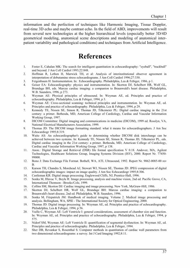
• The method is real-time by nature, as it uses the RF signal, which is only available during image acquisition. Apart from being a unique advantage, this also means the method cannot be used off-line, nor can the same images be re-analyzed with different settings. Whenever RF data can be stored, this limitation will be resolved.

Most of these problems are exemplary for a low-level method that does not use any geometric models or knowledge about cardiac anatomy. Apart from these drawbacks, the use of RF data supplies superior basic information for blood-tissue classification and may well serve as a basis for higher-level developments, especially when the digital RF data becomes available for off-line postprocessing.

The use of Harmonic Imaging (see below) has been shown to improve AQ border delineation58,59, but does not eliminate most of these problems.

A spin-off of AQ is known as Color Kinesis60,61 (Fig. 1.4). This is in essence a method of presenting the time sequence of AQ contours in a single image, by color-coding the lumen area for each time frame and superimposing these. This renders a rainbow-like lumen where each color represents some time-offset from ED. Provided there is little global heart translation, this can give a good impression of wall motion patterns in systole or diastole, especially when these are analyzed per region61-63. Of course, all limitations of AQ apply here as well, plus the concern of overall heart translation, so that this technique is also challenging to apply accurately.

1.4.4.2 Clinical use AQ has been applied in clinical studies for many purposes, especially for looking at left ventricular function (lumen area, volume and fractional area change). Studies on right ventricular function have been reported as well64. Combination of AQ data with invasively measured ventricular pressure has been reported65 allowing pressure-area and pressure-volume loops to be constructed, which may hold promise for the assessment of LV mechanical performance. Color Kinesis has been used for studying wall motion patterns in several patient groups, systolic and diastolic function, regional wall motion in stress echo, etc.63,66,67

1.4.5 Structure based method: matched filters As an example of a structure based method, we highlight the method by Geiser and Wilson24,44,68 for automatically detecting endocardial and epicardial borders in short-axis echocardiograms. The method is based on matched filters that respond to arc-like structures. The first step applies a filter that responds to the bright epicardial/pericardial interface at the posterior wall. Subsequently, other circular structures along the wall are detected and after update of the LV center estimate, redetected (an example of high-to-low level feedback). This gives an estimate of epicardial position, which is used as a region of interest. Radial edge detectors are used to locally adjust epicardial edges and to estimate the (relatively strong) anteroseptal endocardial edge. From the estimated wall thickness, the border search is further limited and final endocardial and epicardial edge estimates are found (Fig. 1.5).

Chapter 1

29

Figure 1.5. Short-axis border detection with arc filters. Top: Short-axis echocardiographic images at end diastole and end systole. Bottom: automatically generated borders at end diastole and end systole. (From: Sheehan F, Wilson DC, Shavelle D, Geiser EA: Echocardiography. In: Sonka M, Fitzpatrick JM, eds. Handbook of medical imaging. Volume 2. Medical image processing and analysis, p 659. Reprinted with permission of SPIE - The International Society for Optical Engineering, Bellingham, WA).

This method seems practically useful (it has been validated on a large set of (quality-selected) patients), and it is clever in the sense that it uses feedback between a high-level model of a short-axis cross section and low-level feature data. From a theoretical viewpoint it is vulnerable because of the cascade of dependent steps, each of which may fail and cause the process to break down. Much of the applied geometrical and expert knowledge (like the order of strength of expected features) seems to be coded into the steps of the algorithm rather than being captured in a general model. Such an approach may be hard to extend to other views or to certain pathologies that break the assumptions, as this requires redesigning the algorithm.

1.4.6 Object based method: Echo-CMS

1.4.6.1 Method As an example of an object based (pattern- and geometric model based) ABD method, we will describe the Echo-CMS® system (Medis medical imaging systems bv, Leiden, the Netherlands) that was developed in our laboratory. The system has been designed for practical use, with the main intent of quantifying endocardial wall motion and lumen volume frame-to-frame. A relatively simple circular-model based dynamic programming approach is used for short-axis views46,56. An LV center point is indicated by the user, defining a circular model and ROI in which the strong endocardial edge is found by Dynamic Programming using first-derivatives and smoothness/distance constraints. The found border is used as a model in neighboring frames to allow frame-to-frame analysis.

Chapter 1

30

Figure 1.6. Echo-CMS semiautomated border detection procedure. From left to right: A. ECG and original images B. Manual drawing of 2 contours and inspection of markers C. Generation of pose models (landmarks) D. Generation of shape models E. Generation of profile models (match patterns) F. Automatically detected contours In the different long axis views (apical four-chamber, two-chamber and parasternal long axis) a more elaborate semiautomated pattern-based approach is used23,69. For the analysis of one ore more complete beats (Fig. 1.6.A), one ED and ES contour must be manually drawn (Fig. 1.6.B). Next, three landmark points characterizing the position of the LV (apex and mitral valve attachment points, which are the end points of the contour) are extracted from the contours and inter/extrapolated linearly over the cycle(s). The user is required to inspect these markers over the cycle(s) and may then redefine, if necessary, intermediate positions where the true position deviates from the estimated position. Now, the automated contour detection is started. From the manually drawn ED and ES contours, models are extracted describing the geometrical shape of the ventricle over the cycle and the intensity profiles in a neighborhood of the drawn contours. All models (phase, pose, geometry and edge profiles) are interpolated over the cycle and extrapolated over other cycles (Fig. 1.6.C,D,E). The resulting geometry models are positioned over the images (Fig. 1.7.B), which are resampled along straight lines perpendicular to the models. For each point of all scan lines (Fig. 1.7.C, left), a cost value is calculated representing the likelihood of this point as a contour point: unlikely points will have high costs. The cost is calculated from a combination of edge detectors, match differences with the edge profile models, and local edge reliability measures. Through this rectangular array of cost values (Fig. 1.7.C, center), an optimal connective path is determined using a Dynamic Programming approach. Cumulative costs for all connective paths are calculated, applying

Chapter 1

31

Figure 1.7. Echo-CMS Dynamic Programming border detection. A. Original image B. Image with landmarks and shape model C. Scan value matrix (left); cost value matrix (middle) and detected path (right) D. Image with detected contour position-dependent penalties for deviation from a straight path. In this way, local stiffness of parts of the border is modeled. The path with overall lowest cost is selected as optimal (Fig. 1.7.C, right) and by inversion of the resampling process converted into a new contour (Fig. 1.7.D).

After detection of all contours (Fig. 1.6.F), the user may apply any corrections by overdrawing part of a contour. Consecutively, all models are updated with the extra user-defined information, which is interpolated and extrapolated over the sequence, followed by a redetection of all non-manual contours.

In short, this method uses full-cycle models for the 2D pose, shape and local stiffness properties of the wall, and for the intensity profiles of the edges. Case-specific and user-specific information is incorporated by collecting information from all user-defined contours. Drawbacks are the need for 2 manually defined borders and the marker manipulations.

Chapter 1

32

1.4.6.2 Clinical use This method has been applied in studies on wall motion patterns for pacemakers70,71 and systolic function72-74. The system has some very strong features, including tracking of structures other than blood-tissue borders (user-defined positions); temporal and spatial coherence; and basic knowledge of LV anatomy and appearance. For research purposes it has been shown to be a valuable tool, but at the moment it is mainly focused on frame-to-frame or multi-beat analyses of wall motion patterns. For ED/ES analyses it offers no extra benefits, as the ED/ES contours need to be defined manually.

1.4.7 Population model based method: Active Appearance Models

A great promise is held by a new class of techniques named Active Appearance Models (AAM). These techniques were originally developed by Cootes et al.75,76 for facial recognition and medical image analysis, as an extension of the Active Shape Model (ASM)42,51,53 approach. We have recently applied AAMs to MRI77 and echocardiograms78 with very promising results. These techniques derive the typical shape and appearance of an echocardiogram from a large set of example images with expert-drawn contours. Principal Component Analysis (PCA) on a Point Distribution Model extracts the average organ shape and the principal shape variations. By warping all examples to the average shape, an average image (Fig. 1.8) and principal image variations (Fig. 1.9) can be found. By applying another PCA simultaneous shape and intensity eigenvariations are modeled, in an Appearance Model. Such an Appearance Model can synthetically generate ‘probable’ echocardiographic images similar to the variations in Fig. 1.9. By deforming the model along the characteristic model eigenvariations using a gradient descent minimization of the difference between the synthetic and the real image, the desired structure can be found (Fig. 1.10). This can be done fast and fully automatically with good results.

This technique has some significant advantages: it models both average organ shape and all variations over a population of examples; it models the complete organ appearance, including typical artifacts; it captures the expert’s definition of proper border definition; it can model complex shapes (e.g. LV endocard plus LV epicard, RV, valves etc.); it is not limited to blood-tissue borders; and it is easily customizable for different types of images. Limitations of this technique are its dependence on the training data, the selected population of examples and the quality of the expert contours.

1.5 Future promise In the near future, serious improvements in the applicability of ABD may be expected. Some instrumental developments will have important effects, and the ABD methods themselves will improve.

Chapter 1

33

Figure 1.8. Active Appearance Model: average four-chamber images of left ventricle from 65 patients, at different moments in the cardiac phase. A. End-diastole B. Mid-systole C. End-systole D. End of rapid filling E. Start of atrial filling

Figure 1.9. Active Appearance Model: AAM eigenvariations 1 to 4 of 4-chamber LV at end-diastole. Left to right: average minus 3 standard deviations, average, average plus 3 standard deviations Top to bottom: AAM eigenvariations 1 to 4. Note the simultaneous shape and intensity variations.

Chapter 1

34

Figure 1.10. AAM matching results on end-systolic LV four-chamber image. A. Image with initial model B. Intermediate iteration C. Final matching result

Chapter 1

35

1.5.1 Impact of instrumental developments

1.5.1.1 Harmonic imaging Any technical measure that improves visual image quality is likely to improve ABD as well. This is certainly true for Harmonic Imaging (HI). Originally intended to be used in combination with contrast, HI has been shown to improve endocardial visualization in 2D echo79 without contrast as well58. It has also been shown to improve endocardial tracking by AQ as rated visually58, and by correlating AQ EF measurements to X-ray ventriculography59. AQ with HI still underestimates absolute volumes and can be technically difficult to perform. Note that HI will not improve image quality in all cases, and that it sometimes results in a very grainy image. ABD techniques that rely on image texture may be influenced, but others should certainly benefit from HI.

1.5.1.2 Tissue Doppler, strain imaging Tissue Doppler (TDI) can supply real-time information on tissue velocity in the direction of the ultrasound beam, and thus in itself is a method for quantification of motion80-83. The derived Strain Rate Imaging84 and Strain Imaging85,86 techniques provide an estimate of local tissue strain, but their practical value remains to be established. For certain purposes, this may become an alternative to border motion detection approaches, but the one-dimensionality of the measurement limits its use considerably. Tissue Doppler information could also well be included into Automated Border Detection techniques, as it provides clues both on presence and local speed of tissue. ABD might supply additional (transversal) motion information.

1.5.1.3 3D/4D ultrasound In principle, 3-D image acquisition may provide superior input data for ABD. Border positions can be detected more reliable if information from neighboring slices can be used: spatial continuity, like temporal continuity, may provide additional clues in difficult-to-interpret cases. Furthermore, real volumes may be calculated from 3-D data instead of monoplane or biplane estimates. However, the triggered acquisition of such image sets may introduce motion artifacts. 3-D smoothing and cut-plane interpolations may also influence border positions. This modality will probably benefit most from an inherently 3-D or 4-D model-based detection technique. Momentarily, real-time 3D ultrasound (RT3D, Volumetrics, Durham NC) is becoming available87,88; this eliminates triggering problems and motion artifacts, but image quality is still limited. With improvement of image quality, RT3D may become an important substrate for ABD.

1.5.1.4 Contrast Ultrasound contrast agents can be used for luminal opacification to improve visualization of the endocardial border, or for myocardial opacification. In contrary to what is sometimes suggested89, it is unlikely that contrast will directly enhance ABD. Although lumen opacification may boost the visual interpretation, application of contrast still has many pitfalls. Especially the transient nature of the opacification, incomplete or inhomogeneous filling of the cavity, shadowing, and local destruction of microbubbles

Chapter 1

36

(causing mixing of ‘white’ and ‘black’ blood) make it hard to model the lumen appearance for any detection method. Next-generation contrast agents or special-purpose border detection techniques may provide solutions.

1.5.1.5 Digital image storage/RF data Digital image storage and communication will have a positive effect on general image quality and the availability of additional information (calibration, time, patient age and sex, BSA, physiological signals, protocol stages, views) can be a highly important source of a priori information for ABD techniques. As soon as raw RF information becomes available via digital storage, digital postprocessing of this data may provide superior input for ABD methods, effectively combining the strengths of AQ with those of high-level model-based approaches.

1.5.2 Developments in image processing

1.5.2.1 Model-based techniques As seen in the section on Active Appearance Models, the biggest promises come from new developments in higher-level image processing. These techniques can model the complete appearance of a cardiac echo scene, including patient variabilities. This may allow more natural solutions than older, edge-based or geometric-model based approaches. As both shape variations over a large patient set and image appearance variations can be modeled, these techniques may handle typical artifacts, locally differing edge patterns, etc., while restricting themselves to probable shapes. Furthermore, it seems possible to separate these models in patient-specific, view-specific and pathology-specific parts90, allowing more precise and flexible models, and opening views to automated classification. The next-generation ABD technique for ultrasound may well emerge from this family.

1.5.2.2 Intelligent systems At the interpretation level, we enter the domain of Artificial Intelligence. Work in this field, especially in conjunction with image interpretation, is still in its infancy. Many high-level interpretation problems will need techniques from AI to be solved: formal reasoning from rule-based expert knowledge; generating multiple hypotheses with measures of confidence; reasoning with pathological/congenital conditions during detection; checking overall consistency of an interpretation, and taking action to resolve conflicts; opportunistically choosing an optimal detection strategy for the image data presented; learning from operator corrections and actions. Ultimately, such developments may lead to an intelligent ‘automated image interpretation assistant’ for echocardiographers.

1.6 Summary Automated border detection for ultrasound is still in full development. Few clinically applicable systems exist, and automation is limited. Positive expectations exist for the future. At the instrumental side, new opportunities will emerge from computer and ultrasound hardware improvements, availability of digital images and of raw RF

Chapter 1

37

information and the perfection of techniques like Harmonic Imaging, Tissue Doppler, real-time 3D echo and maybe contrast echo. In the field of ABD, improvements will result from several new technologies at the higher hierarchical levels (especially better 3D/4D geometrical modeling, anatomical scene descriptions and modeling of anatomical inter-patient variability and pathological conditions) and techniques from Artificial Intelligence.

References 1. Foster E, Cahalan MK: The search for intelligent quantitation in echocardiography: "eyeball", "trackball"

and beyond. J Am Coll Cardiol 1993;22:848. 2. Hoffman R, Lethen H, Marwick TH, et al: Analysis of interinstitutional observer agreement in

interpretation of dobutamine stress echocardiograms. J Am Coll Cardiol 1996;27:330. 3. Feigenbaum H: Instrumentation. In: Echocardiography. Philadelphia, Lea & Febiger, 1986, p 1. 4. Geiser EA: Echocardiography: physics and instrumentation. In: Skorton DJ, Schelbert HR, Wolf GL,

Brundage BH, eds. Marcus cardiac imaging: a companion to Braunwald's heart disease. Philadelphia, W.B. Saunders, 1996, p 273.

5. Weyman AE: Physical principles of ultrasound. In: Weyman AE, ed. Principles and practice of echocardiography. Philadelphia, Lea & Febiger, 1994, p 3.

6. Weyman AE: Cross-sectional scanning: technical principles and instrumentation. In: Weyman AE, ed. Principles and practice of echocardiography. Philadelphia, Lea & Febiger, 1994, p 29.

7. Kennedy TE, Nissen SE, Simon R, Thomas JD, Tilkemeier PL: Digital cardiac imaging in the 21st century: a primer. Bethesda, MD, American College of Cardiology, Cardiac and Vascular Information Working Group, 1997.

8. DICOM Committee: Digital imaging and communications in medicine (DICOM), 1999 ed. Rosslyn, VA, National Electrical Manufacturers Association, 1999.

9. Thomas JD: The DICOM image formatting standard: what it means for echocardiographers. J Am Soc Echocardiogr 1995;8:319.

10. Waitz AS: An echocardiographer's guide to determining whether DICOM disk interchange can be achieved between two systems. In: Kennedy TE, Nissen SE, Simon R, Thomas JD, Tilkemeier PL, eds. Digital cardiac imaging in the 21st century: a primer. Bethesda, MD, American College of Cardiology, Cardiac and Vascular Information Working Group, 1997, p 138.

11. Anon.: Digital Storage and Retrieval (DSR) file format specification V 0.18. Andover, MA, Agilent Technologies, Healthcare Solutions Group, Imaging Systems Division (ISY), 2000. Report Nr. 77450-99000.

12. Bono J: Data Exchange File Format. Bothell, WA, ATL Ultrasound, 1992. Report Nr. 9062-0085-00 rev B.

13. Karson TH, Chandra S, Morehead AJ, Stewart WJ, Nissen SE, Thomas JD: JPEG compression of digital echocardiographic images: impact on image quality. J Am Soc Echocardiogr 1995;8:306.

14. Castleman KR: Digital image processing. Englewood Cliffs, NJ, Prentice-Hall, 1996. 15. Sonka M, Hlavac V, Boyle R: Image processing, analysis and machine vision, 2nd ed. Pacific Grove, CA,

International Thomson - Brooks/Cole, 1999. 16. Collins SM, Skorton DJ: Cardiac imaging and image processing. New York, McGraw-Hill, 1986. 17. Skorton DJ, Schelbert HR, Wolf GL, Brundage BH: Marcus cardiac imaging: a companion to

Braunwald's heart disease, 2nd ed. Philadelphia, W.B. Saunders, 1996. 18. Sonka M, Fitzpatrick JM: Handbook of medical imaging. Volume 2. Medical image processing and

analysis. Bellingham, WA, SPIE - The International Society for Optical Engineering, 2000. 19. Thomas JD: Digital image processing. In: Weyman AE, ed. Principles and practice of echocardiography.

Philadelphia, Lea & Febiger, 1994, p 56. 20. Vuille C, Weyman AE: Left Ventricle I: general considerations, assessment of chamber size and function.

In: Weyman AE, ed. Principles and practice of echocardiography. Philadelphia, Lea & Febiger, 1994, p 575.

21. Nidorf SM, Weyman AE: Left Ventricle II: quantification of segmental dysfunction. In: Weyman AE, ed. Principles and practice of echocardiography. Philadelphia, Lea & Febiger, 1994.

22. Sher DB, Revankar S, Rosenthal S: Computer methods in quantitation of cardiac wall parameters from two dimensional echocardiograms: a survey. Int J Card Imaging 1992;8:11.

Chapter 1

38

23. Bosch JG, van Burken G, Nijland F, Reiber JHC: Overview of automated quantitation techniques in 2D echocardiography. In: Reiber JHC, van der Wall EE, eds. What's new in cardiovascular imaging. Dordrecht, the Netherlands, Kluwer, 1998, p 363.

24. Sheehan F, Wilson DC, Shavelle D, Geiser EA: Echocardiography. In: Sonka M, Fitzpatrick JM, eds. Handbook of medical imaging. Volume 2. Medical image processing and analysis. Bellingham, WA, SPIE - The International Society for Optical Engineering, 2000, p 609.

25. Geiser EA: Edge detection and wall motion analysis. In: Chambers J, Monaghan M, eds. Echocardiography: an international review. Oxford, Oxford University Press, 1993, p 71.

26. Grube E, Mathers F, Backs B, Luederitz B: Automatische und halbautomatische Konturfindung des linken Ventrikels im zweidimensionalen Echokardiogramm. In-vitro Untersuchungen an formalinfixierten Schweineherzen. Z Kardiol 1985;74:15.

27. Ezekiel A, Garcia EV, Areeda JS, Corday SR: Automatic and intelligent left ventricular contour detection from two-dimensional echocardiograms. Proceedings, Computers in Cardiol. IEEE Computer Society Press, Los Alamitos, CA, 1985;261.

28. Klingler JW, Vaughan CL, Fraker TD, Andrews LT: Segmentation of echocardiographic images using mathematical morphology. IEEE Trans Biomed Eng 1988;35:925.

29. Montilla G, Barrios V, Roux C, Mora F, Passariello G: Border detection in echocardiography images using texture analysis. Proceedings, Computers in Cardiol. IEEE Computer Society Press, Los Alamitos, CA, 1992;643.

30. Setarehdan SK, Soraghan JJ: Automatic left ventricular feature extraction and visualisation from echocardiographic images. Proceedings, Computers in Cardiol. IEEE Computer Society Press, Los Alamitos, CA, 1996;9.

31. Verlande M, Flachskampf FA, Schneider W, Ameling W, Hanrath P: 3D reconstruction of the beating left ventricle and mitral valve based on multiplanar TEE. Proceedings, Computers in Cardiol. IEEE Computer Society Press, Los Alamitos, CA, 1991;285.

32. Perez JE, Waggoner AD, Barzilai B, Melton HE, Miller JG, Sobel BE: On-line assessment of ventricular function by automatic boundary detection and ultrasonic backscatter imaging. J Am Coll Cardiol 1992;19:313.

33. Han CY, Lin KW, Wee WG, Mintz RM, Porembka DT: Knowledge-based image analysis for automated boundary extraction of transesophageal echocardiographic left-ventricular images. IEEE Trans Med Imaging 1991;10:602.

34. Hozumi T, Yoshida K, Yoshioka H, et al.: Echocardiographic estimation of left ventricular cavity area with a newly developed automated contour tracking method. J Am Soc Echocardiogr 1997;10:822.

35. Monteiro AP, Marques de Sa JP, Abreu-Lima C: Automatic detection of echocardiographic LV-contours. A new image enhancement and sequential tracking method. Proceedings, Computers in Cardiol. IEEE Computer Society Press, Los Alamitos, CA, 1988;453.

36. Chu CH, Delp EJ, Buda AJ: Detecting left ventricular endocardial and epicardial boundaries by digital two-dimensional echocardiography. IEEE Trans Med Imaging 1988;7:81.

37. Feng J, Lin W-C, Chen C-T: Epicardial boundary detection using fuzzy reasoning. IEEE Trans Med Imaging 1991;10:187.

38. Chalana V, Linker DT, Haynor DR, Kim Y: A multiple active contour model for cardiac boundary detection on echocardiographic sequences. IEEE Trans Med Imaging 1996;15:290.

39. Dong L, Pelle G, Brun P, Unser M: Model-based boundary detection in echocardiography using dynamic programming technique. Proceedings, SPIE Medical Imaging V. SPIE - The International Society for Optical Engineering, Bellingham, WA, 1991;178.

40. Friedland N, Adam D: Echocardiographic myocardial edge detection using an optimization protocol. Proceedings, Computers in Cardiol. IEEE Computer Society Press, Los Alamitos, CA, 1989;379.

41. Belohlavek M, Manduca A, Behrenbeck T, Seward J, Greenleaf JF: Image analysis using modified self-organizing maps: automated delineation of the left ventricular cavity in serial echocardiograms. Proceedings, 4th int conf Visualisation in Biomedical Computing VBC '96. Springer, Berlin, 1996;247.

42. Cootes TF, Hill A, Taylor CJ, Haslam J: Use of active shape models for locating structures in medical images. Image and Vision Computing 1994;12:355.

43. Detmer PR, Bashein G, Martin RW: Matched filter identification of left-ventricular endocardial borders in transesophageal echocardiograms. IEEE Trans Med Imaging 1990;9:396.

44. Geiser EA, Wilson DC, Wang DX, Conetta DA, Murphy JD, Hutson AD: Autonomous epicardial and endocardial boundary detection in echocardiographic short-axis images. J Am Soc Echocardiogr 1998;11:338.

45. Herlin IL, Nguyen C, Graffigne C: Stochastic segmentation of ultrasound images. Proceedings, 11th IAPR Int Conf Pattern Recognition A: Computer vision and applications. IEEE Computer Society Press, Los Alamitos, CA, 1992;289.

Chapter 1

39

46. Bosch JG, Savalle LH, van Burken G, Reiber JHC: Evaluation of a semiautomatic contour detection approach in sequences of short-axis two-dimensional echocardiographic images. J Am Soc Echocardiogr 1995;8:810.

47. Dias JMB, Leitao JMN: Wall position and thickness estimation from sequences of echocardiographic images. IEEE Trans Med Imaging 1996;15:25.

48. Gustavsson T, Molander S, Pascher R, Liang Q, Broman H, Caidahl K: A model-based procedure for fully automated boundary detection and 3D reconstruction from 2D echocardiograms. Proceedings, Computers in Cardiol. IEEE Computer Society Press, Los Alamitos, CA, 1994;209.

49. Maes L, Delaere D, Suetens P, Aubert A, van der Werf F: Automated contour detection of the left ventricle in short axis view and long axis view on 2D echocardiograms. Proceedings, Computers in Cardiol. IEEE Computer Society Press, Los Alamitos, CA, 1990;603.

50. Cohen LD: Note on active contour models and balloons. CVGIP Image Understanding 1991;53:211. 51. Cootes TF, Taylor CJ, Cooper DH, Graham J: Active Shape Models - their training and application. Comp

Vision Image Understanding 1995;61:38. 52. Coppini G, Poli R, Valli G: Recovery of the 3-D shape of the left ventricle from echocardiographic

images. IEEE Trans Med Imaging 1995;14:301. 53. Parker AD, Hill A, Taylor CJ, Cootes TF, Jin XY, Gibson DG: Application of point distribution models to

the automated analysis of echocardiograms. Proceedings, Computers in Cardiol. IEEE Computer Society Press, Los Alamitos, CA, 1994;25.

54. Brotherton T, Pollard T, Simpson P, DeMaria A: Echocardiogram structure and tissue classification using hierarchical fuzzy neural networks. Proceedings, IEEE Conf Acoustics, Speech and Signal Proc. IEEE Computer Society Press, New York, 1994;573.

55. Marcus R, Bednarz J, Coulden R, Shroff S, Lipton M, Lang R: Ultrasonic backscatter system for automated on-line endocardial boundary detection: evaluation by ultrafast computed tomography. J Am Coll Cardiol 1993;22:839.

56. Bosch JG, Reiber JH, van Burken G, Savalle L, Maurincomme E, Helbing WA: Automated contour detection and acoustic quantification. Eur Heart J 1995;16 Suppl J:35.

57. Chandra S, Garcia MJ, Morehead AJ, et al.: Spatiotemporal Fourier filtration of acoustic quantification endocardial border using carthesian vs. polar coordinate system. Proceedings, Computers in Cardiol. IEEE Computer Society Press, Los Alamitos, CA, 1994;17.

58. Spencer KT, Bednarz J, Rafter PG, Korcarz C, Lang RM: Use of harmonic imaging without echocardiographic contrast to improve two-dimensional image quality. Am J Cardiol 1998;82:794.

59. Tsujita-Kuroda Y, Zhang G, Sumita Y, et al.: Validity and reproducibility of echocardiographic measurement of left ventricular ejection fraction by Acoustic Quantification with Tissue Harmonic Imaging technique. J Am Soc Echocardiogr 2000;13:300.

60. Lang RM, Vignon P, Weinert L, Bednarz J, Korcarz C, Sandelski J et al.: Echocardiographic quantification of regional left ventricular wall motion with color kinesis. Circulation 1996;93:1877.

61. MorAvi V, Vignon P, Koch R, Weinert L, Garcia MJ, Spencer KT et al.: Segmental analysis of color kinesis images: New method for quantification of the magnitude and timing of endocardial motion during left ventricular systole and diastole. Circulation 1997;95:2082.

62. Vignon P, MorAvi V, Weinert L, Koch R, Spencer KT, Lang RM: Quantitative evaluation of global and regional left ventricular diastolic function with color kinesis. Circulation 1998;97:1053.

63. Koch R, Lang RM, Garcia MJ, Weinert L, Bednarz J, Korcarz C et al.: Objective evaluation of regional left ventricular wall motion during dobutamine stress echocardiographic studies using segmental analysis of color kinesis images. J Am Coll Cardiol 1999;34:409.

64. Helbing WA, Bosch HG, Maliepaard C, Zwinderman KH, Rebergen SA, Ottenkamp J et al.: On-line automated border detection for echocardiographic quantification of right ventricular size and function in children. Pediatr Cardiol 1997;18:261.

65. Gorcsan J, Romand JA, Mandarino WA, Deneault LG, Pinsky MR: Assessment of left ventricular performance by on-line pressure-area relations using echocardiographic automated border detection. J Am Coll Cardiol 1994;23:242.

66. Carey CF, Mor A, V, Koch R, Lang R, Perez JE: Effects of inotropic stimulation on segmental left ventricular relaxation quantified by color kinesis. Am J Cardiol 2000;85:1476.

67. Mor-Avi V, Spencer KT, Lang RM: Acoustic quantification today and its future horizons. Echocardiography 1999;16:85.

68. Geiser EA, Wilson DC: Automatic center point determination in 2-dimensional short-axis echocardiographic images. Pattern Recognition 1992;25:893.

69. Bosch JG, van Burken G, Reiber JHC: Automatic frame-to-frame contour detection in echocardiograms using motion estimation. Proceedings, Computers in Cardiol. IEEE Computer Society Press, Los Alamitos, CA, 1992;351.

Chapter 1

40

70. Auricchio A, Ghanem A, Groethus F, et al: Echocardiographic analysis of left ventricular contraction patterns in left bundle branch block and congestive heart failure. Abstract. J Cardiac Failure 1999;5(3, suppl. 1):3.

71. Breithardt OA, Kramer A, Schiffgens B et al: Characteristics of left ventricular contraction patterns and acute changes with multisite pacing in patients with heart failure as assessed by echocardiographic semiautomatic contour detection. Abstract. Eur Heart J 2000;21(Abstract suppl.):351.

72. Fry SJ, Hunziker PR, Bosch HG, Reiber JHC, Picard MH: Automated echocardiographic confirmation of regional wall motion abnormalities: quantitation of continuous LV volume. Abstract. J Am Coll Cardiol 1998;31(2 suppl. A):56A.

73. Hunziker PR, Schöb L, Lefkovits M, et al: Automatic border detection in dobutamine stress echo: how do normal and ischaemic segments behave objectively and quantitatively? Abstract. Eur Heart J 1999;20(Abstract suppl):618.

74. Hunziker PR, Yuan D, Schöb L et al: Objective and quantitative stress echo analysis to diagnose coronary disease using model-based image processing. Abstract. J Am Coll Cardiol 2000;35(2(suppl A)):413A.

75. Cootes TF, Edwards GJ, Taylor CJ: Active Appearance Models. Proceedings, European Conf Computer Vision. Springer, Berlin, 1998;2:484.

76. Edwards GJ, Taylor CJ, Cootes TF: Interpreting face images using Active Appearance Models. Proceedings, 3rd Int Conf Face and Gesture Recognition. Japan, 1998;300.

77. Mitchell SC, Lelieveldt BPF, van der Geest RJ, Schaap J, Reiber JHC: Segmentation of cardiac MR images: an active appearance model approach. Proceedings, SPIE Medical Imaging 2000, Image Processing. SPIE - The International Optical Engineering Society, Bellingham, WA, 2000;3979:224.

78. Bosch JG, Mitchell SC, Lelieveldt BPF et al: Feasibility of fully automated border detection on stress echocardiograms by Active Appearance Models. Abstract. Eur Heart J 2000;21(abstract suppl):11.

79. van Camp G, Franken PR, Schoors D, Hagers Y, Koole M, Demoor D et al.: Impact of second harmonic imaging on the determination of the global and regional left ventricular function by 2D echocardiography: a comparison with MIBI gated SPECT. Eur J Echocardiography 2000;1:122.

80. Isaaz K: What are we actually measuring by Doppler tissue imaging? J Am Coll Cardiol 2000;36:897. 81. Hunziker PR, Picard MH, Jander N, Scherrer CM, Pfisterer M, Buser PT: Regional wall motion

assessment in stress echocardiography by tissue Doppler bull's-eyes. J Am Soc Echocardiogr 1999;12:196.

82. Derumeaux G, Ovize M, Loufoua J, Pontier G, Andre F, X, Cribier A: Assessment of nonuniformity of transmural myocardial velocities by color-coded tissue Doppler imaging - Characterization of normal, ischemic, and stunned myocardium. Circulation 2000;101:1390.

83. Pasquet A, Armstrong G, Beachler L, Lauer MS, Marwick TH: Use of segmental tissue Doppler velocity to quantitate exercise echocardiography. J Am Soc Echocardiogr 1999;12:901.

84. Heimdal A, Stoylen A, Torp H, Skjaerpe T: Real-time strain rate imaging of the left ventricle by ultrasound. J Am Soc Echocardiogr 1998;11:1013.

85. Armstrong G, Pasquet A, Fukamachi K, Cardon L, Olstad B, Marwick T: Use of peak systolic strain as an index of regional left ventricular function: Comparison with tissue Doppler velocity during dobutamine stress and myocardial ischemia. J Am Soc Echocardiogr 2000;13:731.

86. Urheim S, Edvardsen T, Torp H, Angelsen B, Smiseth OA: Myocardial strain by Doppler echocardiography - Validation of a new method to quantify regional myocardial function. Circulation 2000;102:1158.

87. Qin JJX, Jones M, Shiota T, et al.: New digital measurement methods for left ventricular volume using real-time three-dimensional echocardiography: comparison with electromagnetic flow method and magnetic resonance imaging. Eur J Echocardiography 2000;1:96.

88. Takuma S, Zwas DR, Fard A, Wu H, Chaudhry H, Di Tullio MR et al.: Real-time, 3-dimensional echocardiography acquires all standard 2-dimensional images from 2 volume sets: A clinical demonstration in 45 patients. J Am Soc Echocardiogr 1999;12:1.

89. Kamp O, Sieswerda GT, Visser CA: State-of-the-art. Stress echocardiography entering the next millennium. In: Reiber JHC, van der Wall EE, eds. What's new in cardiovascular imaging. Dordrecht, the Netherlands, Kluwer, 1998, p 351.

90. Costen N, Cootes TF, Edwards GJ, Taylor CJ: Simultaneous extraction of functional face subspaces. Proceedings, IEEE computer vision & pattern recognition. IEEE Computer Society Press, Los Alamitos, CA, 1999;492.

41

Chapter 2

Evaluation of a semiautomatic

contour detection approach in sequences of short-axis two-dimensional

echocardiographic images.

J.G. Bosch1, L.H. Savalle2, G. van Burken1, J.H.C. Reiber1.

1Division of Image Processing, Department of Radiology, Leiden University Medical Center, Leiden, The Netherlands.

2Department of Cardiology, Leiden University Medical Center,

Leiden, The Netherlands.

J Am Soc Echocardiogr 8 (1995): 810-821.

Chapter 2

42

Abstract Quantitative analysis of echocardiographic sequences has been limited by time-consuming and strenuous manual tracing approaches. To circumvent these disadvantages, we have developed the EchoCardiographic Measurement System (ECHO-CMS). ECHO-CMS employs the robust, model-based Minimum Cost Contour Tracking technique for semi-automatic detection of left ventricular (LV) endocardial contours in sequences of consecutive echocardiographic images. An evaluation study was carried out on 20 short-axis patient studies (10 transesophageal and 10 transthoracic studies), each consisting of 16 consecutive images covering approximately one cardiac cycle.

The LV endocardial contours in the 320 images were analyzed both by manual tracing and semiautomatically. In addition, inter-observer and intra-observer variabilities were determined for both techniques in two patients (32 images). Manual editing was required in only 57 (18%) of all 320 contours detected. Average processing time per patient for manual tracing was 25 minutes (of which 18½ minutes was for drawing and corrections), and for semiautomatic tracing it was only 5½ minutes (of which just 1½ minutes was for corrections). Regression analysis showed excellent correspondence between manual and semiautomatic tracing: semiautomatic = 1.01*manual + 5.58%; r = 0.989, standard error of the estimate = 11.9% (n = 320 contours). Inter-observer and intra-observer variabilities were smaller for semiautomatic than for manual tracing, although not in all cases statistically significant. In conclusion, semiautomatic LV short-axis endocardial contour detection by ECHO-CMS provides contours that are highly similar to those drawn by an expert; it is five to 10 times faster than manual tracing and reduces intra-observer and inter-observer variabilities. This demonstrates that ECHO-CMS is a useful tool for clinical echocardiographic research studies.

Chapter 2

43

2.1 Introduction 2.1.1 Need for objective quantification of wall motion Two-dimensional echocardiography allows the real-time inspection of the wall motion of the heart over many cardiac cycles. By far most echocardiographic examinations are used for qualitative diagnostic purposes only. Quantitative analysis of echocardiographic images has been shown to provide many clinically relevant parameters1,2. However, quantitative analysis remains unpopular, because it requires in general manual tracing of contours, which is strenuous and time-consuming and subject to intra-observer and inter-observer variabilities3-6. Most manual analyses are restricted to end-systolic (ES) and end-diastolic (ED) images1,7.

However, these ES/ED analyses address only a small portion of the information on cardiac function that may be derived from the full cardiac cycle. Cross-sectional echocardiography was recognized early on as a reliable method for the detection of the presence and location of regional asynergy associated with acute myocardial infarction8. There is evidence that knowledge of the endocardial contours only at end systole and end diastole is not sufficient: important wall motion abnormalities may remain undetected and in some cases dyskinetic segments may be missed completely9. This implies that analysis of all images in the cardiac cycle (i.e. frame-to-frame contour detection) is necessary for a proper quantitative assessment of left ventricular wall motion. Only a few truly quantitative wall motion studies have been published1,2,9; most wall motion studies, including stress echocardiographic protocols10, are based on qualitative and semiquantitative assessment (i.e. eyeball scoring on a 4- or 5-point scale) of wall motion abnormalities. Automated, objective quantification of wall motion changes in the different stages of a pharmacologic or physical stress echocardiographic protocol may greatly improve the quality of clinical decision making. Frame-to-frame quantitative analysis may be important for patient monitoring as well. It has been shown that acute ischemia causes visible wall motion abnormalities in transesophageal echocardiograms (TEE) long before any S-T segment changes are noted in the electrocardiogram. As a result, TEE seems superior to the electrocardiogram for the detection of intraoperative myocardial ischemia and should allow early identification of patients at higher risk of postoperative cardiovascular complications11,12. Also, TEE is more suitable for detecting intraoperative myocardial ischemia than the widely used pulmonary capillary wedge pressure measurement13.

Therefore, echocardiography (especially TEE) may also be very valuable as a patient-monitoring technique. For practical applicability, however, automatic frame-to-frame contour detection would be required, preferably in real time. Regional endocardial wall motion (as opposed to overall luminal area) should be monitored to detect wall motion abnormalities under these circumstances.

Chapter 2

44

2.1.2 Automated contour detection approaches The technique that momentarily best satisfies the above mentioned requirements is the Acoustic Quantification technique14,15. Because this is a pixel-classification technique rather than a true contour-detection technique, only overall blood area can be calculated, not regional wall motion. Although it is hampered by several limitations and problems, it supplies valuable clinical information in real time16,17.

Several other automated approaches for frame-to-frame contour detection in echocardiograms have been reported,18 but none of these has gained practical acceptance yet. Their applicability is generally limited to superior-quality images or has not been demonstrated on a representative set of routinely acquired images.

As a result, no reliable method exists at this time for the automated frame-to-frame quantification of regional wall motion in echocardiographic images. Commercially available techniques either provide insufficiently accurate borders, or are not capable of supplying quantitative wall motion information. Therefore the rationale for further developments in approaches to frame-to-frame contour detection persists. Features of such a technique should include: (1) frame-to-frame contour detection, extensible to real-time performance; (2) generation of contour position and motion information, both globally and regionally (not just blood-tissue edges or blood areas); and (3) model-based approach, adaptable to different types of edges and features.

A method for automated contour detection with the above-mentioned features has been developed in our laboratory in the past years19,20. It is known as the Minimum Cost Contour Tracking (MCCT) method. The MCCT technique provides continuous, connective, smooth contours that allow regional wall motion calculations, volume estimations, user corrections etc., in both single frames and frame-to-frame analysis. In this article the advantages and limitations of this MCCT technique are presented, based on the results from an evaluation study carried out on routinely acquired clinical materials.

2.2 Methods and material 2.2.1 EchoCardiographic Measurement System

(ECHO-CMS) The MCCT method has been implemented in an off-line echocardiographic analysis workstation developed in our laboratory: the EchoCardiographic Measurement System* (ECHO-CMS) (Fig. 2.1). It consists of an IBM-compatible personal computer (486/25MHz was used in this study) equipped with a frame grabber (Imaging Technology Variable-Scan Frame Grabber; Imaging Technology, Bedford, Mass.) for digitization and display of images, two color monitors, and a mouse. ECHO-CMS can either digitize images from an analog video source (typically a VCR or the video output of an ultrasound scanner) or import digital images (e.g., from an optical disk unit). A time-base corrector is used to provide adequate synchronization when digitizing still-frame VCR images.

The ECHO-CMS program has been implemented as an MS-Windows application, which provides a familiar, standardized, and versatile user interface, allowing user-

* Commercialized by Medis medical imaging systems bv, Dungense Kant 12, Nuenen, the Netherlands.

Chapter 2

45

Figure 2.1. Diagram of ECHO-CMS system. ECHO-CMS consists of PC (486 or Pentium), frame grabber, two monitors and mouse. Images are acquired from VCR or directly from ultrasound scanner. friendly, intuitive control over the various elements of the analysis process. The ECHO-CMS system is controlled mainly with the mouse; a trackball or digitizer board may be used as an alternative.

Both automated contour detection and manual tracing of contours are supported, as well as manual correction of contours and propagation of corrections (forward or backward) over a range of images. This allows semiautomatic detection of large numbers of contours with minimal effort and a high degree of user control. The user may apply the automated contour detection by either positioning a geometric model on the image (e.g., a circle with a fixed radius for the short-axis cross sections discussed here) or pre-drawing an approximate contour.

2.2.2 Minimum Cost Contour Tracking MCCT is a flexible contour detection technique that employs models for the contours to be detected and allows frame-to-frame detection, as well as forward or backward propagation of model information and manual corrections. It is based on dynamic programming21, a well-known mathematic technique for determining an optimal solution to logistics problems. In general, it can be applied to any problem that can be formulated in terms of finding an optimal path through a network of points, which is highly relevant to contour detection.

The steps of the MCCT procedure are illustrated in Fig. 2.2. The MCCT technique requires model information representing the approximate shape and position of the contour to be detected. This model may be a contour found in a previous image, a user-drawn approximation, a geometric shape (like a hemiellipse for the left ventricle in the four-chamber view) or a combination of these. The image is resampled along scan lines

Chapter 2

46

Figure 2.2. Different steps of MCCT procedure. A. Image is resampled along scan lines perpendicular to contour model (circle). B. Scan lines are placed in rectangular array, scan matrix. C. Cost matrix is generated by assigning cost value to each point in scan matrix. Cost value is inversely proportional to probability that specific point belongs to desired contour. D. Path through cost matrix is found by dynamic programming technique. E. Path is spatially transformed back into image, interpolated, and smoothed to provide new contour. perpendicular to this model (Fig. 2.2.A). These scan lines are placed in a rectangular array (Fig. 2.2.B). To each point in this array, a cost value is assigned (Fig. 2.2.C). This cost value is inversely proportional to the probability that the specific point belongs to the desired contour. Different types of information may be included in the cost value, e.g., gray value, several measures of edge strength (e.g., first derivative value), distance from the model, etc. Furthermore, factors are used that specify the allowed raggedness of the edge and the propagation of the previous shape in subsequent images.

By the dynamic programming technique, the path with overall minimal cost values is found (Fig. 2.2.D). This path is spatially transformed back into the image, interpolated, and smoothed, to provide the new contour (Fig. 2.2.E).

Because the MCCT process starts and ends with a contour, it can be used in an iterative manner. A rough contour can be used to find a more detailed one, or a contour from a previous image may serve as a model in the next image. Also, a corrected contour may be used as a model to propagate the manual correction over a number of images.

2.2.3 Evaluation setup To assess the speed, robustness, and reproducibility of the MCCT approach, an evaluation study was carried out on 20 patient studies (10 transthoracic echocardiograms (TTEs) and 10 TEEs). Each study consisted of 16 consecutive short-axis cross sections at the midpapillary level, on which semiautomatic and manual contour delineations were compared. Issues of interest were (1) time required for the analysis process, (2) validity of contours, (3) required user interaction, and (4) inter-observer and intra-observer variabilities.

The hypothesis investigated in this study was the following: the semiautomatic MCCT method can provide contours equivalent to manually traced contours, in a fraction of the time necessary for manual tracing. The primary test is the decrease in analysis time, under the condition that semiautomatic contours are not structurally different from manual contours.

Chapter 2

47

The patient studies were selected from videotapes of routinely acquired images from six hospitals in the Netherlands covering a range of echocardiographic equipment (four different brands), image qualities, diseases, and operator settings. Studies included anterior wall infarcts, hypertrophy, dobutamine stress, and TEE-pacing protocols, patients in the intensive care unit with cardiac complications, valvular disease, and normal subjects. Although no explicit grading of image quality was applied, the sequences had to be technically adequate and suitable for visual identification of the endocardium by manual tracing. This criterion did not result in a set of studies with superior image quality: several sequences featured significant dropouts and high noise levels, as well as valvular and trabecular structures. Observers marked some of the sequences as difficult to analyze because of the image quality.

For each patient study, one cardiac cycle was selected of which 16 consecutive images (time interval of 40 msec according to standard European (PAL) video system) were digitized into matrix sizes of 256² pixels (8 bit/pixel) by the ECHO-CMS system; each set of images constituted approximately one cardiac cycle. Each digitized run began at end diastole and ended in the last part of diastole (diastasis) or at the beginning of the next cardiac cycle, depending on the specific heart rate. The sets were stored digitally and used both for the manual and the semiautomatic delineation of the endocardial contour.

The endocardial contours were first drawn manually in all 320 images by the first observer: a cardiologist who was not familiar with the system development and who had only received instructions on the operation of the system. The observer could review the traced contours in cineloop and edit the contours until he was satisfied with the results. Contours were traced to the inner gray value edge, excluding papillary muscles from the luminal area. The final version of the contours after manual editing (contour set Manual) were saved, as well as measured contour areas (in image pixels). The time involved in the drawing of each contour was recorded, as well as the total analysis time per patient study (including loading of images from disk and reviewing of cineloops).

After a period of 7 days, the contours were detected semiautomatically with the MCCT approach by the first observer. A standardized procedure for the semiautomatic contour detection was applied in this study to allow comparisons. The observer indicated the approximate center point of the left ventricle in the first image of the sequence. A general geometric model for the contour to be detected (a circle, for the short-axis view) was positioned relative to this point. As a start, all contours were detected automatically and saved directly. Consecutively, the observer inspected the sequence in a cineloop for erroneous contour parts requiring improvement. If present, an erroneous contour part was corrected manually in only one of the images involved, followed by an automated redetection in the remainder of the images, based on this new model. This step was repeated until all contours were approved by the observer and saved (contour set Semiautomatic). The number of corrections per image and the time involved in the corrections were recorded, as well as the luminal areas of the contours, and total analysis time as above. An example of one image with the manually drawn and automated contours (without corrections) is shown in Fig. 2.3.

After a period of 6 weeks, the manual and semiautomatic tracing procedures were repeated by the first observer for two patient studies (one TEE and one TTE, for a total of 32 images), and carried out for the first time by a second observer who was familiar with the system development (contrary to the first observer). From these data, inter-observer and intra-observer variabilities could be assessed. The contours and derived values from the semiautomatic analysis were compared with the manual results. Comparisons were done separately for the groups of TEE and TTE patient studies and for the total group of

Chapter 2

48

Figure 2.3. Typical short-axis TEE image with endocardial contours. A. Image without contour. B. Image with manually defined contour (from manual set). C. Image with semiautomatically defined contour (from semiautomatic set). No corrections

were applied.

Chapter 2

49

20 patients. Also, the number of corrections and redetections per image was tabulated. Area comparisons were calculated in image pixels, not square millimeters, because the scales of images were different and the comparison was focused on the validity of the contours, not on true areas. Because scales were not varying widely, statistical results will generally apply to true areas as well. Some statistics are expressed in percentages of the average area; this was the average area of all the manual contours: 1565 pixels. Total range of the areas was from 115 to 6135 pixels. Fractional area change was also studied: fractional area change is widely used in echocardiography as a measure of overall heart function based on the ES and ED contours (fractional area change = (EDA - ESA) / EDA, with EDA = ED area, ESA = ES area).

2.3 Statistics Linear regression and correlation coefficients were used to assess the correspondences between manual and semiautomatic contour areas. Furthermore, paired area differences were used to compare manual and semiautomatic contours and to assess intra-observer and inter-observer variabilities. For the area differences between pairs of corresponding contours, the statistics systematic difference (SysDif) and random difference (RanDif) were used. SysDif was defined as the average of paired (signed) differences between corresponding contour areas (e.g., between manual and semiautomatic contours) or between corresponding contours in the inter-observer or intra-observer study. RanDif was defined as the standard deviation of these paired differences. From these measures a confidence interval for the expected difference can easily be calculated (e.g., as SysDif ± 2*RanDif/√n for a 95% confidence interval of the average of n differences.

A p value <0.05 was generally used for tests of statistical significance (or lower if mentioned otherwise). Three different types of significance tests were performed. To test whether a SysDif was statistically significantly different from 0 (e.g., in an intra-observer study), a paired Student t test (two-tailed) was used. To test whether RanDifs were smaller for semiautomatic than for manual, a one-tailed F test was used; because RanDifs are standard deviations, the ratio of their squares was tested against a table of critical values of the F distribution.

To find significant differences between SysDif values (i.e., to show that intra-observer SysDifs are smaller for semiautomatic than for manual contours), an unpaired one-tailed Student t test was used.

2.4 Results 2.4.1 Analysis time Processing time with the MCCT automatic detection procedure proved to be significantly shorter than by the manual tracing procedure (Table 2.1). Total semiautomatic analysis time for the 20 patients was 4.7 times shorter than by manual drawing, which took about 8½ hours for the 320 contours. The time spent specifically on the actual contour drawing, correction, and redetection was even 11.3 times shorter: less than 2 minutes per patient study, instead of almost 20 minutes for the manual procedure. The remaining time was spent on loading the images and viewing the cineloop and the contours.

Chapter 2

50

Table 2.1. Analysis time per patient

(average of 20 patients, 16 contours each)

Drawing, detections, corrections (min) Total analysis time (min) Automatic 1.65 5.42 Manual 18.58 25.22

Table 2.2.

Comparison of manual and semiautomatic contour areas based on 20 patient studies

Areas (n = 320 contours)

Absolute area (pixels)

Relative area (% of average manual area)

FAC (%) (n=20 patients)

Manual contour areas Average 1565 100 69.8 SD 11.1 Semiautomatic Average 1668 106.6 67.3 contour areas SD 11.5 Manual-semiautomatic SysDif -103.2 * -6.6* 2.51 paired differences RanDif 184.9 11.8 5.7 Semiautomatic & Slope (a) 1.010 0.91 manual regression Intercept (b) 87.3 5.6 3.95 and correlation† SEE 185.1 11.9 5.9 r 0.989 0.874

FAC, Fractional area change; SEE, standard error of the estimate. * p < 0.05 † x=manual; y=semiautomatic.

2.4.2 Comparison of manual and automatic contour areas An excellent correlation (r = 0.989) and linear regression relation (a = 1.010, b = 87.3 (5.6% of average area)) were found between the manual and semiautomatic contours (Fig. 2.4). This implies that the semiautomatic contour areas correlated very well with those from the manually traced contours. This is to be expected in a setting in which both the manual and semiautomatic contours were under full control of the observer; it primarily proves that the observer could obtain semiautomatic contours equivalent to the manual contours with limited user interaction. More precise information was obtained from the SysDif and RanDif data calculated for the paired area differences between manual and semiautomatic sets (Table 2.2). Although the systematic difference (-6.6% of average area) is significantly different from 0 (p < 0.001), it is still small. The negative SysDif implies that the semiautomatic contours were slightly larger than the manual ones, which is also apparent from the regression equation. The RanDifs (SD of paired differences) were found to be 11.8%. The magnitude of these differences can partially be explained by intra-observer variability, which is described below.

2.4.3 Fractional Area Change Fractional area change was found to be nearly identical (differences not significant) for the manual and semiautomatic sets (Table 2.2). From the SysDif of paired differences of fractional area changes, it is apparent that the fractional area changes from the semiautomatic method were only marginally smaller (2.51%; p > 0.05). The range of this

Chapter 2

51

Figure 2.4. Linear regression of semiautomatic (SA) contour areas versus areas derived from manual (MAN) contour tracings. Slope a = 1.010, intercept b = 87.3 pixels.

Table 2.3a. Manual corrections

Manual Corrections No Yes Total No. of images 263 57 320 % Images 82.2 17.8 100

Table 2.3b.

Redetections

No. of redetections 0 1 2 >2

No. of images 63 151 59 47 % Images 19.7 47.2 18.4 14.7

Table 2.4.

Inter-observer and intra-observer variabilities measured in two patients (32 images)

Variabilities Intra-observer (%) Inter-observer (%) (n = 32) SA MAN SA MAN SysDif 1.74* 2.91 1.97† 8.44* RanDif 4.18‡ 8.54 4.95 5.45

Significance tests, p < 0.05. SA, semiautomatic; MAN, manual. *SysDif ≠ 0 †SysDif SA < SysDif MAN ‡RanDif SA < RanDif MAN

Chapter 2

52

variation, described by the RanDif, remains small (5.7%) relative to the SD of the total sets of fractional area changes (11.1% and 11.5%, respectively). The SysDif implies that the area overestimation in semiautomatic contours was slightly larger at end systole than at end diastole. Good correlation (r = 0.87) and regression (a = 0.91, b = 3.95%) were found, considering the small number of measurements (n = 20), the narrow range of the fractional area change parameter, and the well-known fact that fractional area change is a derived parameter in which errors accumulate.

2.4.4 Number of corrections and redetections To tabulate the amount of user interaction involved, two types of interactions were registrated: (1) the number of images in which a direct manual correction was applied (i.e., drawing a corrected contour piece manually) and (2) the number of redetection iterations applied to any image. A manual correction was generally used to start a redetection over (a part of) the sequence. The number of redetections is a measure of the success of the semiautomatic approach. Many contours could be (re)detected successfully without needing direct manual corrections.

In 263 (82.2%) of 320 contours, no direct manual corrections were needed (Table 2.3a). In other words, in the vast majority of the images, adequate contours were obtained by automated detection or redetection, without explicit manual corrections. However, in many cases a redetection of part of the image sequence was required (after a manual correction in only one contour) to obtain accurate contours (Table 2.3b). 66.9% of the contours could be found without or with only one redetection and 85.3% within two iterations. Because the MCCT contour detection approach is model driven, an accurate contour for the first image is very important. In this study this first contour was detected with no more information than a center point indicated by the user. In 15 cases of the 20 studies a manual correction to the first contour had to be made, after which the entire sequence was redetected automatically. Only in a small minority of the images were small additional corrections required in a second iteration.

Of course the number of corrections and redetections is dependent on the observer’s skills and familiarity with the program, which is normal for an interactive situation like this. Because the experiments were performed mainly by an unskilled observer, results will only improve with skill.

2.4.5 Inter-observer and intra-observer variability Inter-observer and intra-observer variabilities for the two patient studies are given in Table 2.4. The semiautomatic contours proved less subject to observer variations than did manual sets in all cases, although this was statistically significant only for inter-observer SysDif and intra-observer RanDif. As was to be expected, the inter-observer variations were generally larger than intra-observer variations, except for the inter-observer manual RanDif, which was rather low.

SysDif should approximate 0, especially for an observer variability study. A high SysDif value means that systematically larger contours were traced in one of the two repetitions. Inter-observer manual SysDif was significantly different from 0 (p < 0.01); intra-observer semiautomatic SysDif was significant at p < 0.05, but not at p < 0.01.

Chapter 2

53

Figure 2.5. Linear regression of semiautomatic (SA) contour areas versus areas derived from manual (MAN) contour tracings for TEE and TTE studies. A. TEE. Slope a = 0.983, intercept b = 105.6 pixels. B. TTE. Slope a = 1.031, intercept b = 76.9 pixels.

Chapter 2

54

Table 2.5. Intra-observer and inter-observer variabilities of TEE and TTE

(each one patient, 16 images)

Variabilities Intra-observer (%) Inter-observer (%) (n = 16 each) SA MAN SA MAN SysDif TEE 0.87 -2.87 -0.31† 10.23* RanDif TEE 2.68‡§ 6.25§ 2.81‡§ 4.86 SysDif TTE 2.61 2.96 3.63 6.65* RanDif TTE 5.68‡ 10.82 7.09 6.04

Significance tests, p < 0.05. See Table 2.4 for abbreviations. *SysDif ≠ 0 †SysDif SA < SysDif MAN ‡RanDif SA < RanDif MAN §RanDif TEE < RanDif TTE

2.4.6 Differences between TEE and TTE images The comparisons described above were also performed separately for the group of TEE and TTE studies. In Fig. 2.5, linear regression relations and correlations are shown for TEE and TTE studies. In Table 2.5, intra-observer and inter-observer variabilities for TEE and TTE studies are summarized. Few apparent differences were seen; results were comparable to the overall results. SysDif was significantly different from 0 only for manual inter-observer variabilities (for both TEE and TTE). RanDif was significantly smaller for semiautomatic than for manual variabilities except for TTE inter-observer variabilities. SysDif and RanDif were slightly better in TEE sequences (RanDif mostly significantly), probably because of better image quality. Also, slightly fewer redetections were required in TEE images. In conclusion, MCCT automatic detection seems to work well in both types of sequences.

2.5 Discussion There is a definite need for quantitative analysis of echocardiographic image sequences for the assessment of left ventricular function. However, in practice this is limited by the tedious task of manual tracing of all the contours, which is also subject to observer variabilities. Although some (semi) automated approaches may be available at individual research institutes for their own clinical research studies, no single automated technique has been accepted as yet and distributed on a larger scale.

In an attempt to provide a practical solution to this image processing and analysis problem, we have developed and implemented the MCCT approach on the ECHO-CMS system. As mentioned earlier, the MCCT is a well-known mathematic technique for determining optimal solutions to logistics problems. It has been used, for example, to solve the problem of the traveling salesman who has to visit many cities and find the most efficient way to do so in terms of distance, time spent, travel expenses, etc. Hence the name minimal cost; it is also known as dynamic programming.

This study demonstrates that the MCCT method provides an easy and rapid way to process large numbers of contours. It was found that in 263 (82.2%) of the total number of 320 contours analyzed, no direct manual corrections were needed. The reduction of required processing time by a factor of 5 to 10 is an essential benefit of ECHO-CMS and

Chapter 2

55

implies practical feasibility of frame-to-frame wall motion studies. Random differences between manual and automatic contours could be contributed mainly to observer variability in both manual and semiautomatic contours.

From a comparison of the enclosed area values, it could be concluded that at the average the semiautomatic contours were defined slightly larger than the manually traced ones, resulting in a SysDif of 6.6% of the average area values. Which of the measurements better approaches the truth can only be concluded from a study in which these values would be compared to known areas or volumes (e.g., phantom or cast studies). The inter-observer and intra-observer data were definitely in favor of the semiautomatic approach. The SysDifs between the inter-observer and intra-observer measurements were smaller than those for the manual tracings, particularly for the inter-observer case. This demonstrates one of the great strengths of an automated approach: it is more consistent than two expert observers. The manual intra-observer data show that the SysDif was small (2.91%) and the RanDif rather high (8.54%). This implies that on average small differences were found between contours, although individual cases deviated considerably. A high SysDif value implies that in one of two observations, areas were consistently larger (e.g., because of the systematic inclusion of a particular detail in one observation that was excluded in the other observation).

The manual interobserver data demonstrate that one of the observers consistently drew larger contours than the other, with a relatively small RanDif value. It is very clear that the semiautomatic results for the intraobserver and interobserver studies were associated with small SysDifs (<2%) and very acceptable RanDifs (<5%). Both types of errors proved to be smaller than those for manual analysis, although this was not significant in all cases.

In other studies, intra-observer and inter-observer variabilities in manual area measurements in short-axis images were reported to be typically around 10%3-6, which was confirmed by this study.

Considering the intra-observer RanDifs, it becomes clear that a large part of the RanDif of the paired differences between manual and semiautomatic data may be explained from the intra-observer variabilities. Intra-observer variabilities of both manual (RanDif 8.54%) and semiautomatic approaches (RanDif 4.18%) contribute to the manual-semiautomatic RanDif (Table 2.2: 11.8%). Assuming that the intra-observer RanDifs (of two patients) are good estimations of the general variability for the full set of patients, this would account for a manual-semiautomatic RanDif of 9.51% on the basis of intra-observer variability alone.

Another conclusion can be drawn from the inter-observer results. The first observer was not familiar with the system development and only instructed in the use of the system. The second observer was indeed familiar with the development. The data from Table 2.4 show that no significant systematic inter-observer differences were found by the semiautomatic approach; on the other hand, the manual processing indeed showed systematic differences. The RanDifs were comparable between the two approaches. This implies that familiarity with the program does not seriously influence the tracing results.

Although some user interaction (in the form of corrections) is still necessary, the semiautomatic contours are equivalent to manually drawn contours and are less subject to observer variabilities.

2.5.1 Limitations This study was limited in a number of ways: only relatively short sequences were analyzed (16 images) with limited image resolution (256 × 256 pixels). This was done to

Chapter 2

56

limit both storage space and processing time; in a future study, longer sequences at full-size resolution will be used. The current version of the ECHO-CMS allows the analysis of sequences of more than 100 images at a resolution of 512². In this study, only contour areas have been compared, not contour shape. However, because both manual and semiautomatic contours were under user control and visually similar, results based on shape measurements are expected to be comparable.

Furthermore, this study is limited by the number of patients and observers and does not systematically address the influence of differences in image quality. However, the results seem general enough to support the conclusions given.

2.5.2 Sources of problems in MCCT technique The following remaining sources of problems in the MCCT technique were noted during the evaluation study. Detection of the very first frame in a sequence is still the weakest point of the current implementation of the MCCT. When an erroneous contour part is detected in the first frame, this error will often propagate through the whole sequence. Frequently a small manual correction in the first frame would suffice to detect adequate contours in the full sequence. In a practical situation, the user will indeed process one frame, apply any necessary corrections to the detected contour, and then start the detection for the rest of the sequence. This was not allowed in this study; to obtain a uniform speed measurement for all studies and obtain full information on MCCT performance, the study protocol was standardized. After the definition of the center point, a full detection over all images was performed, followed by corrections and redetections. Probably a practical protocol as sketched above would increase speed and reduce the number of required corrections.

Other problems may occur in the ES phase of the cardiac cycle. The contour may become very small and deformed in this phase. Especially papillary muscles and trabeculae are pressed against each other and the wall, causing the model information to become unreliable. Tracking of the endocardium may be lost in some cases, especially when it is moving outward rapidly. Backward propagation from the following ED frame towards the ES frame solved this problem in most cases. Also, this problem can be solved in a future software release by adding knowledge of general phase-related contour deformation to the detection algorithm.

Very large endocardial shape deviations caused difficulties in the tracking. In one patient this was the cause for several manual corrections. An adaptation of one of the parameters of the MCCT technique could solve the problem; however, for this study a fixed set of parameters was used.

Correction of small details through the full sequence was sometimes cumbersome. The correction propagation method was optimized for larger corrections; an additional propagation method for small corrections seems useful.

2.5.3 Comparison with other methods The general setup of this evaluation study was comparable to some other edge detection algorithm evaluation studies3,22, especially the study performed by Geiser et al.3 A comparable number of patient studies and contours was processed. Our study was less focused on observer variabilities; two instead of five observers were used, and only a subset of patients was analyzed repeatedly. In both studies, similar results for the inter-observer and intra-observer variabilities in manual drawing were found. Also, the

Chapter 2

57

similarity between manual contours and automated contours found with the method of Geiser et al. is comparable to our results. However, results cannot be compared directly, because the two methods were not tested on the same set of images.

The method of Geiser et al. used a priori information and user input as well: three fully manually drawn contours (per cycle per patient, in an average of 27 images) to generate areas of search and restrict deviations. This amount of manual contour input is comparable to the 18% of contours needing partial corrections in our method.

In the study of Geiser et al.,3 images were differentiated in three image quality classes and results were computed per quality class. This was not done in our study, but inclusion criteria of studies and differentiation of sources seems comparable. For the rest, image quality is difficult to standardize; a reference set of images would be needed for comparison purposes.

MCCT performs much faster (about 10 seconds per sequence on 486/25MHz) than the method of Geiser et al. (4 minutes, system unknown). This may partially be due to increased computer speed.

2.5.4 Comparison to Acoustic Quantification At this moment the commercially available Acoustic Quantification technique is the most widespread and best-known method for automated border detection in echocardiography. It provides real-time luminal area and area change information but no wall motion information. The technique employs a 3.2 µsec integration time over which each radiofrequent A line is analyzed to obtain an integrated backscatter image rather than a conventional ultrasound image14,15. Because the two-dimensional integrated backscatter image is considerably smoothed and averaged and speckle noise reduced, it can be used to classify image pixels as blood, tissue or boundary pixels in real time. The user manually outlines a region of interest in the image; pixels labeled as blood within this region of interest can be counted in real time. This allows blood area (A), change of area over time (dA/dT) and fractional area change to be calculated and displayed in graphs in real time. In selected cross sections, volume graphs can be generated as well by applying a single-plane modified Simpson’s rule volume estimation.

Acoustic Quantification is certainly a powerful technique with great clinical value. However, it is not a panacea: it does not provide information on regional wall motion (although it may be extended in this direction) and cannot detect other structures that are not blood-tissue interfaces, like the epicardium. Also, it excludes papillary muscles and trabecular structures from the luminal area, which is not in correspondence with the recommendations of the American Society of Echocardiography.23 This is assumed to be a reason for the area and volume underestimations found in comparisons with manually drawn areas as well as with true volume.16

Furthermore, it is hampered by its dependence on the user-defined, fixed region of interest, which is problematic in case of significant motion of the septum or valvular plane.16 It is highly sensitive to time-gain compensation and lateral gain compensation settings16,17; it can only be used during the echocardiographic examination (on-line) because it is incorporated in the front end (radiofrequency part) of the ultrasound machine. Therefore it does not allow off-line analysis or retrospective analysis and it lacks adequate contour-correction facilities.

Although this study does not provide a comparison with Acoustic Quantification, the MCCT method shows that there are alternatives to Acoustic Quantification that may overcome many of its limitations. Although not all limitations of Acoustic Quantification

Chapter 2

58

are eliminated by the MCCT method as described in this paper, it is not limited principally by them. Furthermore, combinations of Acoustic Quantification with MCCT are viable, because MCCT may use the edge information supplied by Acoustic Quantification, in that way combining the advantages of both techniques.24

MCCT can either exclude or include papillary muscles, depending on parameter settings. The Acoustic Quantification technique, however, cannot eliminate the papillary muscles. In this study we had chosen to exclude them from the lumen, because at the midpapillary level it is often difficult to indicate an exact border between myocardial and papillary tissue. This extra source of observer variability would complicate the study unnecessarily. The MCCT method, however, can deal quite well with papillary muscles (detached or not), mitral valve apparatus, trabeculae, intracavitary structure and artifacts, etc. Intracavitary structure and artifacts were in fact present in several images and did not pose special problems.

2.6 Conclusions In conclusion, quantitative echocardiographic left ventricular analysis in the ECHO-CMS system, with a model-based contour detection technique, provides contours that are similar to those drawn by an expert observer, is 5 to 10 times faster than manual tracing, and is characterized by reduced intra-observer and inter-observer variabilities. This allows ECHO-CMS to become a useful tool for clinical research studies.

Acknowledgements We thank L. Baur, MD, B. Delamarre, MD, E.J. Gussenhoven, MD, J.P.M. Hamer, MD, O. Kamp, MD, E. Pieper, MD, C. Peels, MD, C.A. Visser, MD, and W.B. Vletter, who supplied patient data that were used in this study.

References 1. Force TL, Folland ED, Aebischer N, Sharma S, Parisi AF. Echocardiographic assessment of ventricular

function. In: Marcus ML, Skorton DJ, Schelbert HR, Wolf GL, eds. Cardiac imaging: a companion to Braunwald's heart disease. Philadelphia: W.B. Saunders, 1991:375-401.

2. Mann DL, Gillam LD, Weyman AE. Cross-sectional echocardiographic assessment of regional left ventricular performance and myocardial perfusion. Prog Cardiovasc Dis 1986;29:1-52.

3. Geiser EA, Oliver LH, Gardin JM, et al. Clinical validation of an edge detection algorithm for two-dimensional echocardiographic short-axis images. J Am Soc Echocardiogr 1988;1:410-21.

4. Moynihan PF, Parisi AF, Feldman CL. Quantitative detection of regional left ventricular contraction abnormalities by two-dimensional echocardiography, I: Analysis of methods. Circulation 1981;63:752-60.

5. Parisi AF, Moynihan PF, Folland ED, Feldman CL. Quantitative detection of regional left ventricular contraction abnormalities by two-dimensional echocardiography, II: Accuracy in coronary artery disease. Circulation 1981;63:761-7.

6. Wyatt HL, Haendchen RV, Meerbaum S, Corday E. Assessment of quantitative methods for two-dimensional echocardiography. Am J Cardiol 1983;52:396-401.

7. Feigenbaum H. Echocardiography. 4th ed. Philadelphia: Lea & Febiger, 1986. 8. Heger JJ, Weyman AE, Wann LS, Dillon JC, Feigenbaum H. Cross-sectional echocardiography in acute

myocardial infarction: detection and localization of regional left ventricular asynergy. Circulation 1979;60:531-8.

Chapter 2

59

9. Weyman AE, Franklin TD, Hogan RD, et al. Importance of temporal heterogeneity in assessing the contraction abnormalities associated with acute myocardial ischemia. Circulation 1984;70:102-12.

10. Quiñones MA, Verani MS, Haichin RM, Mahmarian JJ, Suarez J, Zoghbi WA. Exercise echocardiography versus 201-Tl single-photon emission computed tomography in evaluation of coronary artery disease: analysis of 292 patients. Circulation 1992;85:1026-31.

11. Smith JS, Cahalan MK, Benefiel DJ, et al. Intraoperative detection of myocardial ischemia in high-risk patients: electrocardiography versus two-dimensional transesophageal echocardiography. Circulation 1985;72:1015-21.

12. Gibson RS, Bishop HL, Stamm RB, Crampton RS, Beller GA, Martin RP. Value of early two dimensional echocardiography in patients with acute myocardial infarction. Am J Cardiol 1982;49:1110-9.

13. van Daele MERM, Sutherland GR, Mitchell MM, et al. Do changes in pulmonary capillary wedge pressure adequately reflect myocardial ischemia during anesthesia? A correlative preoperative hemodynamic, electrocardiographic, and transesophageal echocardiographic study. Circulation 1990;81:865-71.

14. Perez JE, Klein SC, Prater DM, et al. Automated on-line quantification of left ventricular dimensions and function by echocardiography with backscatter imaging and lateral gain compensation. Am J Cardiol 1992;18:205-12.

15. Perez JE, Waggoner AD, Barzilai B, et al. On-line assessment of ventricular function by automatic boundary detection and ultrasonic backscatter imaging. J Am Coll Cardiol 1992;19:313-20.

16. Morrissey RL, Siu SC, Guerrero JL, Newell JB, Weyman AE, Picard MH. Automated assessment of ventricular volume and function by echocardiography: validation of automated border detection. J Am Soc Echocardiogr 1994;7:107-115.

17. Smith MD, Xie GY, Sapin PM, et al. Factors affecting the determination of left ventricular area by acoustic quantitation [Abstract]. J Am Coll Cardiol 1992;19:299A.

18. Sher DB, Revankar S, Rosenthal S. Computer methods in quantitation of cardiac wall parameters from two-dimensional echocardiograms: a survey. Int J Cardiac Imaging 1992;8:11-26.

19. Bosch JG, Reiber JHC, van Burken G, Gerbrands JJ, Roelandt JRTC. Automated contour detection on short-axis transesophageal echocardiograms. In: Erbel R, Khanderia BK, Brennecke R, Meyer J, Seward JB, Tajik AJ, eds. Transesophageal Echocardiography. A new window to the heart. Berlin: Springer, 1989;253-259.

20. Bosch JG, Reiber JHC, van Burken G, et al. Developments towards real-time frame-to-frame automatic contour detection on echocardiograms. Comput Cardiol 1990; 435-8.

21. Gerbrands JJ. Segmentation of noisy images. Thesis, Delft University of Technology, June 1988. 22. Grube E, Backs A, Backs B, Luderitz B. Automatische Konturerkennung im zweidimensionalen

Echokardiogramm: Untersuchungen an einem algemeinen Patientenkollektiv. Z Kardiol 1985;74:445-52. 23. Shah PM, Crawford M, DeMaria A, et al. Recommendations for quantitation of the left ventricle by two-

dimensional echocardiography. J Am Soc Echocardiogr 1989;2:358-67. 24. Bosch JG, Reiber JHC, van Burken G, Savalle LH, Maurincomme E. Automated contour detection and

acoustic quantification. Eur Heart J 1995; 16 (Suppl J): 35-41.

Chapter 2

60

61

Chapter 3

Automated contour detection in

echocardiographic image sequences using dynamic programming, pattern matching

and spatiotemporal geometric models.

Johan G. Bosch1, Gerard van Burken1, Francisca Nijland2, Jan M. van Dantzig3

and Johan H.C. Reiber1

1Division of Image Processing, Department of Radiology, Leiden University Medical Center, Leiden, The Netherlands.

2Department of Cardiology, Vrije Universiteit Medical Center,

Amsterdam, The Netherlands.

3Department of Cardiology, University Hospital Maastricht, Maastricht, The Netherlands.

Chapter 3

62

Chapter 3

63

3.1 Introduction Automated quantitation in two-dimensional (2D) echocardiography has been a field of continuous research since the advent of cardiac echo itself. The limitations of a visual assessment of cardiac parameters from ultrasound images have been widely acknowledged1. E.g., visual wall motion scoring as practiced in stress echocardiography is associated with large variabilities2.

Quantitative analysis requires a reliable and reproducible detection of endocardial borders of the left ventricle. Outlining the borders of the cardiac wall is essential for calculation of volumes, wall motion and thickness. Automatic border detection (ABD, also known as contour detection or automatic delineation) would eliminate the tedious manual tracing, which is highly subject to inter- and intra-observer variability. Unfortunately, automating the border detection in cardiac ultrasound is a difficult and underestimated task.

Perception and interpretation of images is a very complicated task in general. Humans perform it extremely well; therefore they amply underestimate its complexity. Interpretation of medical images, especially of a complex, dynamic organ like the heart is still more difficult, as it requires expert knowledge of the three-dimensional anatomical structures in the heart, their dynamical behavior, pathology and anatomical variability between patients, and the intricacies of the imaging modality involved. This last point specifically should not be underestimated for ultrasound. The problems - both in general and specific for ultrasonography - are further discussed in chapter 1 of this thesis and in the introductions of chapters 2, 4, 5 and 6. An extensive overview of different techniques for automated endocardial border detection is also given in chapter 1 of this thesis.

Despite continuous efforts of numerous research groups, no ‘silver bullet’ technique for automatic quantitation in echocardiography has evolved yet. A number of useful and promising methods have been developed and have been used in clinical practice, but fully automated, unsupervised analysis of echocardiograms is still a distant goal.

In this chapter, we describe multiple practically applicable techniques that we have developed for semiautomatic border detection of the left ventricle in sequences of echocardiograms, and their evaluation. These techniques were implemented in the Echo-CMS system (which was commercialized by Medis medical imaging systems bv, Leiden, the Netherlands), an off-line analysis system for automated border detection in echocardiographic image sequences. The system and its applications are described in ch. 2 and 7 of this thesis.

3.2 Methods 3.2.1 Border detection as a graph search problem The task of detecting borders of an object in an image can be treated in many ways: as a pixel-labeling problem, as an iterative deformation problem, as a shape-matching problem etc. (see ch. 1). In this chapter, we will look at the detection of the border of an object as a graph search problem. Many methods have been developed for finding an optimal path through a graph (a network consisting of nodes and arcs between nodes, each with certain

Chapter 3

64

properties). If we can formulate our detection problem as a graph and the properties of nodes represent local image properties related to a border, then we can use graph search techniques to find a path corresponding to our desired contour. As we will see, this is a powerful approach that can be relatively flexible and robust.

3.2.2 Concepts of Dynamic Programming The methods described in this chapter all make use of variants of Dynamic Programming3 (DP), a well-known graph search technique stemming from the field of Operations Research. DP finds the optimal path through a network of nodes in a particularly effective manner. It was initially applied to border finding in images by Montanari4 and Martelli5. A good overview of the classical application of DP for segmentation is given by Gerbrands6. In Fig. 3.1, the technique is explained. DP works on a special class of networks, consisting of nodes that are arranged as a rectangular matrix X of R rows and K columns. Each node Xr,k at row r and column k is connected only to a limited number q = (2s+1) of neighboring nodes Xr+1,k’ on the next row, where k’∈ { k-s , ... , k+s}; s is the allowed ‘sidestep’ (Fig. 3.1.A, with s=1). We will call such a matrix q-connective. One can traverse the matrix of nodes from start row 1 (bottom) to end row R (top) by going from any node on the start row to any of its q-connected neighbors on the second row, and from there to any of its neighbors on the third row, etc. Each resulting path p = ( X1,k(1) , X2,k(2) , ... , XR,k(R) ) (Fig. 3.1.B) is uniquely described by its R-dimensional index vector k = ( k(1) , ... , k(R) ), will contain exactly one node pr = Xr,k(r) on each row r and will be q-connective, e.g. consecutive path nodes are never more than s columns apart (Eq. (3.1)). | k(r+1) – k(r) | ≤ s for ∀r ∈ {1 , ... , R-1} (3.1) A cost value Cr,k is assigned to each node (and possibly also to each arc that connects two nodes). For this example, costs are assigned to nodes only (Fig. 3.1.A). The total cost T(p) of a path p is defined as the sum of all node (and arc) costs (Fig. 3.1.B, Eq. (3.2).

( )∑=

=R

rrkrCT

1,)( p (3.2)

The task at hand is to find the path pmin (Fig. 3.1.F) for which the total cost T(p) is minimal (Eq. (3.3)). Hence, DP is also often referred to as ‘minimum cost path search’ or ‘minimum cost algorithm’ (MCA). Figure 3.1. Dynamic Programming (facing page). A. Array of R*K nodes with costs assigned to nodes; q-connectivity for q=3, s=1 (per node, 3

connections to neighbors on next row). B. Example of a q-connective path p (bold nodes and arcs) with total cost T(p). Node costs

given within nodes; partial cumulative costs Tr,k(r) of path on right upper side of each path node.

C. Example of forward search (resulting in suboptimal path). D. Example of picking best candidates per row (resulting in non-connective path). E. Dynamic programming: forward cumulative cost calculation. From bottom to top, for all

nodes a best partial cumulative cost Tr,k and a reference to its predecessor node (bold arrows) are stored.

F. Dynamic programming: backtracking of optimal path pmin from best node (2) on row R.

Chapter 3

65

Chapter 3

66

( ))(minargmin pp

pT

∀= (3.3)

This may seem a simple problem at first glance, but the solution requires some ingenuity. A brute-force comparison of the costs of all possible paths is extremely time consuming for all but the smallest matrices (complexity of order K*qR, with q≥3 and R>100 typically). A basic forward search (plainly choose the best q-connective candidate on the next row) will in most cases not find the minimal cost solution, as is obvious from our simple example (Fig. 3.1.C). Finally, picking the nodes with lowest cost on each row (Fig. 3.1.D) is not a valid approach either, because it is unlikely to result in a q-connective solution that satisfies Eq. (3.1). Several methods are known to find the optimal solution of Eq. (3.3); DP is one of them. It is a breadth-first heuristic search method, closely related to its depth-first cousin, the A*-algorithm7. For the described special class of regular networks, DP is particularly effective. Its essential notion is, that for each node X on the optimal path pmin = AB, the partial paths A (from Start to X) and B (from X to End) must also be optimal. This is easily proven by reductio ad absurdum: (1) AB is the optimal path from Start to End; X is a node on this path.

(2) Assume there is a different partial path C from X to End with lower cost than B. Then, the total path AC would have lower cost than AB. This is in contradiction with (1).

(3) Therefore, no partial path C with lower cost than B can exist (Q.E.D.).

This means, that for each node Xr,k there is an optimal partial path from Start to Xr,k. That partial path pr,k and its total cost Tr,k is all we need to know during the solving of our problem. We can forget about any other paths between Start and Xr,k. Furthermore, if we know the optimal paths and costs for all nodes on row r, it is easy to find the optimal paths for row r+1, because for a certain node Xr+1,k, there are only q possible predecessors (Fig. 3.1.E), for each of which the cost of the partial optimal path Tr,j is already known. The cost Tr+1,k of the optimal path from Start to Xr+1,k is therefore simply

jrskskjkrkr TCT ,,,,1,1 min+−=++ +=

K (3.4)

For each node Xr,k we store the partial cumulative cost Tr,k and an index to the predecessor node. We know the minimal cumulative costs for each node of the start row; this is the cost of the node itself:

T1,k = C1,k (3.5) So by combining Eq. (3.4) and (3.5), we can calculate the minimal costs for all nodes on the second row, and by induction, for all rows. This is illustrated in Fig. 3.1.E.

When we have arrived at the end row, the optimal path is simply found by backtracking (Fig. 3.1.F). We pick the node with overall lowest cost (in the example, this is node XR,2). This is the end node of the optimal path, and we look up its predecessor node; from the predecessor, we look up its predecessor etc. and the total optimal path is

Chapter 3

67

reconstructed. The method is guaranteed to find the optimal solution, and complexity is of order K*q*R, dramatically lower than the brute-force approach.

3.2.2.1 From image to graph network and back In our border detection applications, the nodes in the rectangular arrays represent positions in an image, the node costs represent the local image features (somehow related to the contour we want to detect, e.g. local edge strength) and the found path is the optimal contour, given the cost function and connectivity restrictions we apply. In general, the image samples are taken only from a part of the image, the region where we want to find a contour. See Fig. 3.2 for illustration. In the image (Fig. 3.2.A), an estimate for the contour (a ‘model’) is placed (Fig. 3.2.B). In a strip around this estimate, the image is resampled and the values are placed in the rectangular array (Fig. 3.2.C, left). This can be done by an actual warping of the target region into the rectangular array, or by sampling along scanlines perpendicular to the model. In all cases, one should ensure that the sampling gives an adequate representation of the image features. Minimally, proper smoothing or low pass filtering should be used to prevent aliasing; bilinear or other 2D interpolation can be used for sampling at non-integer pixel positions.

Classically, resampling is applied to the image itself, which results in a rectangular scan matrix; feature extraction for generating the cost matrix (Fig. 3.2.C, mid) is performed in the resampled scan matrix, mostly by applying convolution filters. This has the advantage of reduced data processing, and allows feature extraction at the proper resolution and in the proper direction with respect to the expected edges (important for edge detection). However, it is also possible to process the original image first for feature extraction, and resample the result. This is to be preferred for operations that may suffer from distortions in the image grid or local scale changes, such as smoothing, line detectors, and scale-dependent edge detectors (e.g., Canny8).

After generating the cost matrix, the optimal path can be found by DP (Fig. 3.2.C, right). Note that each node in the graph corresponds to a discrete point in the image. The solution space is therefore limited to these discrete points. A detected path therefore corresponds to a sequence of these points; generally, some interpolation is used to derive a connective contour in the original image coordinate system (Fig. 3.2.D).

3.2.2.2 Properties of the DP optimal path The DP optimal path has some elegant properties:

1. If the search through the cost matrix is performed in the reverse direction, the found optimal path will be identical. This is logical, since the cost of the path is the sum of the cost of its nodes. This is a desirable property in case of object contours, where the found border should not depend on the direction of search.

2. If a fixed offset C0 is added to all node costs, the optimal path will not change; total cost of all paths will increase with R*C0.

3. If a fixed offset Cr is added to all node costs of one row, the optimal path will not change. Total cost of all paths will increase with Cr.

4. If all node costs are ≥0, multiplying all node costs by a positive factor F0 will not change the optimal path. Total cost is multiplied by F0. This condition can always be fulfilled by using property 2, with C0 ≤ min(Cr,k).

Chapter 3

68

Figure 3.2. Standard DP (Minimum Cost) application for contour detection. A. Original image B. Image with landmarks and shape model C. Left: scan matrix. Mid: cost matrix. Right: detected path D. Image with detected contour These properties enhance the robustness of DP, because the optimality is insensitive to general linear changes in the cost function output. If the cost function uses linear operators on images (e.g. convolutions), global changes in image contrast or brightness will not influence the results.

Furthermore, the optimality is relatively insensitive to noise and small disturbances; the total cost difference between the optimal path and any “second best” candidate path determines the stability of the solution. Even in very noisy conditions, the strong features are still accurately found and the path only deviates locally in regions with very poor edge definition, which is often practically very acceptable6.

Chapter 3

69

3.2.3 Dynamic Programming variations in border detection

While the basis of DP is simple and well known, an enormous number of variations are possible, some of which apply special restrictions or additions to the basic concept, others ‘change the rules’.

3.2.3.1 Forcing a path through a node A straightforward restriction is forcing the path to start or end at a certain node, or to pass through one or more nodes. This can simply be enforced by setting the costs of all other nodes of the particular row(s) to infinite (or sufficiently high values, in practice) and running a standard DP. More elegantly, a penalty can be applied to any nodes outside a certain neighborhood. Such a penalty can be a complex combination of figures of merit as well, like the distance to the preferred position, image features, distance from a model, etc. We have applied this for fitting a best smooth path to a number of (possibly conflicting) support points9, as described below in 3.2.3.5.

3.2.3.2 Finding a closed path Another common variation is finding the optimal closed contour, in case the model is a closed shape (such as a circle or a blob). In that case, an optimal closed path is desired: the start and end node are required to be adjacent (q-connected), and the constraint of Eq. (3.1) is extended into Eq. (3.6). | k(1) – k(R) | ≤ s ∧ | k(r+1) – k(r) | ≤ s for ∀r ∈ {1 , ... , R-1} (3.6) In our case, closed contours are desired in short-axis echocardiographic images.

A simple but computationally expensive solution requires that for each node on the start row, all non-adjacent nodes on the end row are masked. This brute-force solution requires K complete DP runs. Of the K resulting paths (all closed) the one with lowest cost is the optimal closed path.

A fast and practical solution only uses maximally 2 DP runs; however, it is not guaranteed to find the optimal closed path in all cases. Here, a standard optimal path (not necessarily closed) is first found with DP; if start and end are adjacent (Eq. (3.6) is satisfied), the optimal closed path is already found. If this is not the case, along one of the middle rows the matrix is cut and the start row is made q-connected to the end row. For the new start and end row, the position where the optimal path crossed is enforced (by masking the other nodes). Now, a second DP run finds a closed path, which is presumed to be optimal or very close to that. This works very well if the cost information is known to be very reliable around the row where the matrix is cut. This is indeed the case for short-axis images, where the edges are most prominent near the upper and lower points of the lumen, due to the perpendicular incidence of the ultrasound beams.

Our lab has also developed a solution that is guaranteed to be optimal and has a complexity between 1 and K DP runs (depending on the data and allowed sidestep s)10,11. Because of the higher implementational complexity of this approach, mostly either the previous suboptimal solution or the brute-force solution is used.

Chapter 3

70

3.2.3.3 Finding a path in 3 or more dimensions A simple extension to finding a path in multiple dimensions is possible. In the standard 2-dimensional case, we find a path through a sequence of R rows of size K with q-connectivity; in the 3D case, we find a path through a sequence of R rectangular matrices of size Kx*Ky with qx*qy-connectivity; in 4D, the path traverses a sequence of R cubes of size Kx*Ky*Kz with qx*qy*qz connectivity, etc. The positions in these matrices can represent positions in images, but also in an arbitrary parameter space. In all cases, a singular optimal path of R points with q-connectivity in all dimensions is found. One application is tracking of an anatomical landmark in two dimensions (x,y) over time; another was described by Sonka12 for simultaneous detection of a pair of interrelated contours. Costs at points (k1,k2,r) in a cube (sequence of matrices) are defined as a function of both the costs from a conventional two-dimensional DP cost matrix for the first contour (k1,r dimensions) and the other contour (k2,r dimensions). Finding the 3D path in the r direction and projecting it back onto k1,r and k2,r planes will simultaneously give the two 2D paths for both interrelated contours (p.194 in13). A similar approach has been used in our lab by Dijkstra et al.14 for simultaneous detection of longitudinal vessel contours in IVUS sequences.

3.2.3.4 Finding a plane (or multiple connective paths) in 3 dimensions Many researchers have tried to extend dynamic programming to finding a minimum-cost connective plane in a 3-dimensional cube of nodes. This would correspond to finding contours in a number of consecutive planes (in space or time), which are connective between planes and form the optimal overall set. Although this may look like a straightforward extension, it is easy to show that the connectivity in two dimensions makes it impossible to apply the essential notion of a partial optimal solution and use a similar form of induction as described by Eq. (3.4) and (3.5). A row-by-row approach, covering the plane by a spiral, meander or other pattern all fail because they break the assumptions for optimality, or cannot guarantee connectivity, or result in explosive complexity (each path of R points in plane y of the cube has Rq valid neighbor paths in plane y+1; q≥3).

Partial solutions to this problem have been formulated (e.g.15) in which pairs or triplets of contour points from neighboring planes are combined into single nodes, which are interconnected in a more complex way. This has been shown to be feasible for finding connective contours in 2 to 5 planes simultaneously, but the complexity explodes for more than 3 planes.

Recently, a general solution for this problem has emerged. It was inspired by a different part of graph theory and involves computing minimum s-t cuts in graphs16. This appears very promising for finding optimal solutions to many medical image segmentation problems.

Obviously, such a solution has not been used in the methods described below. In general, connectivity of contours between consecutive time frames was induced either by using the previous contour as a model in the next frame (a form of “forward search” not guaranteed to lead to an optimal solution) or by postprocessing (temporal smoothing of contours).

Chapter 3

71

3.2.3.5 Cost functions In the classical DP-based border detection, costs are mostly defined from low-level image features, e.g. the output of edge detectors (generally simple convolution filters). Often, also other components are introduced, such as distance from an expected position. Such cost components can easily be combined (e.g. as weighted sums) but the weighting can have dramatic effects on the results.

However, a cost function can also be defined from very different information, such as local correspondence to some border template, a priori likelihood of presence of an edge, or co-occurrence of other objects. Therefore, the quality of the result in DP-based methods does not depend on the DP algorithm itself, but on the applied parameters and restrictions, and especially on the composition of the cost function.

A general problem lies in the weighting of model-based and image-based terms. Translation of image features into cost terms is generally realized in a straightforward manner, e.g. by a fixed weighting term or by normalizing to some output range estimate. In practice, differences in image features (contrast, brightness, noise) make it often hard to perform a proper weighting between cases. Cost terms that represent shape properties (e.g. distance from the model, contour smoothness etc) are mostly from a very different order. Balancing shape-based cost terms against image-dependent terms is not trivial. In fact, the problems are similar to the balancing of internal and external forces in snake or balloon approaches17. The DP approach, however, has a definite advantage over a snake-like approach, because it is guaranteed to find an optimal solution instantaneously (given the model, cost function etc.); it is not an iterative method and lacks the typical problems of convergence, stopping criteria, local minima etc.

An elegant application is relating node costs to probabilities. If for each node a probability Pr,k can be estimated that this node is part of the path, DP provides a way of finding the path with overall highest probability. Intuitively, probability of a path should be proportional to the product of the probabilities of its nodes. If we model our cost as Cr,k = – log (Pr,k), the total cost of a path is

∏∑∑===

−=−==R

rrkr

R

rrkr

R

rrkr PPCT

1)(,

1)(,

1)(, )log()log()( p (3.7)

which is indeed proportional to the product of the probabilities of its nodes. As additional constraints, probabilities should be between 0 and 1, and the sum of all probabilities per row must be exactly 1, because the path must pass through one of the nodes.

⎪⎭

⎪⎬⎫

=

≤∀≤

∑=

1

10

1,

,K

kkr

kr

P

P (3.8)

A row r’ that has absolutely no preferences for any node, should have a uniform probability distribution: Pr’,k = 1/K for ∀k .

An example of such a probability-based cost function is given in9, where we used dynamic programming to fit a smooth contour to a number of possibly conflicting support points. Here, probability of each node as being part of the path was composed of multiple Gaussian probability distributions, of which the height and width were determined by probability and proximity of the support points (Fig. 3.3).

Chapter 3

72

Figure 3.3. Probability-based cost function for fitting a smooth contour to a number of possibly conflicting support points (from9). A. Cost matrix, with a landscape plot representing the cost values generated from the distances

to the support points. B. Resulting fit through support points by DP.

3.2.3.6 Smoothness of paths The sidestep parameter s limits the maximally allowed tortuosity of the path, but it is not very useful for controlling the smoothness of the path, since it is an integer value mostly set to 1 or 2. In general, we want to control smoothness in a more subtle way. The path should follow strong edges accurately, but in noisy regions it should not jump around to follow all peaks in the noise. A popular way of controlling the smoothness of the detected contours is by introducing a penalty for ‘sidestepping’ in the path search. If such a penalty (“sidestep cost”) is high, paths will tend to be mostly straight and the detected contour will look much like a scaled version of the model. If the penalty is 0, no adherence to the model’s shape is applied; only the allowed sidestep limits the deviation. The penalty can even be negative, stimulating a zigzag-type path and a winding border. As above, if this penalty is simply a fixed value, it is very hard to properly normalize this value with respect to the current costs.

Sometimes the use of a multiplicative penalty is advocated, so a sidestep effectively increases the cost of the target node with a constant factor. This can be advantageous, since for low-cost (reliable) path sections the extra sidestep cost will have little influence, while in relatively high-cost regions, the sidestep cost will be large and the path will tend to become straight. In that way, the penalty normalization problem is circumvented, and the cost of sidestepping will always be in accordance with the feature strength. However, one can show that such multiplicative penalties inhibit all four of the aforementioned

Chapter 3

73

elegant properties of the DP solution. Therefore, a multiplicative penalty should be applied with care and only after costs are properly normalized to a fixed positive range.

A more flexible and elegant approach is to assign explicit costs to the arcs between nodes in the network. Such costs can then be generated from image information or model information, and localized, weighted or normalized at will, just like node costs.

3.2.3.7 Iterative approaches Since the DP approach starts and ends with a contour, it can be applied iteratively. This means that a detected contour is used as a model in a following iteration, possibly with adjusted parameters. Starting with a rough model and coarse resampling over a broad range, a rough approximation of a contour can be detected, which again serves as a model for a higher-resolution resampling over a narrow band around the model. In this way, an accurate and detailed border can be found with low computational demand; also, this allows the detection of highly winding, non-convex shapes. This is impossible with a single-step approach and a convex, smooth model because of the sidestep limitation. This approach has been applied throughout our developments, starting with the early single-frame detection approaches for TEE18-20 and IVUS21,22. A similar approach is used for feed-forward detection in sequences: from the border detected in an image, a model is constructed which is used in neighboring images. This is based on the assumption that shape change between consecutive images is sufficiently limited.

In our research, we have concentrated on finding well-matched cost functions for our problem, that exploit the optimality of DP contour finding; generating good geometrical models; and including pattern matching approaches into the cost functions, to make best use of the information that can be extracted from expert-defined contours. Furthermore, we have dealt with forcing contours through fixed positions, finding closed contours, and imposing local stiffness to parts of the path. We also have incorporated reliability measures of the feature extraction into our cost measures.

3.2.4 DP detection with pattern matching: MCCT

3.2.4.1 Limitations of edge-based endocardial border detection The original detection approach for short-axis image sequences is described in detail in chapter 2 of this thesis. It uses closed-contour dynamic programming (see 3.2.3.2) with an edge-based cost function and requires only the indication of a center point of the left ventricle, or the manual drawing of a first contour approximation. A feed-forward geometric model prediction (3.2.3.7) is used: the contour detected in one image is smoothed and used as the model for the next and/or previous image. The width of the search range is adapted to the expected maximal frame-to-frame wall displacement.

In major-axis cross sections (apical four-chamber, apical two-chamber, parasternal long axis), similar approaches have been applied (see chapter 7.2.2) but with limited success. In major-axis images, two specific issues make detection of the endocardium more difficult than for short-axis images:

1. The geometric model is more complex: a hemi-elliptic, open shape, with complex dynamic behavior (e.g. the moving mitral valve plane).

2. The border appearance (intensity patterns) can be very different per region; and the strongest edge is often not the desired one. Edges are obscured by noise, artifacts, dropouts etc. Often, the cardiologist wants to track a structure that is

Chapter 3

74

not associated with an edge at all (e.g. because of trabecular structure, imaging artifacts, or foreshortening).

The second issue (diversity of edge patterns, inhomogeneity) is very typical for ultrasound, where standardization of image generation is particularly hard to achieve. Apart from normal anatomical variations, this is specifically due to the strong influence of operator-dependent choice of image cross section and regional gain settings, and to the patient-dependent acoustic windows and artifacts. Therefore, for echocardiography it is very difficult to formulate general properties of the appearance of edges and regions that are valid for all regions and all patients.

Initially, the technique described above for short-axis detection was extended in a straightforward way towards major-axis images, addressing only the first issue. Instead of a single center point, three markers were used: an apical marker and two mitral valve points. A hemi-elliptic model was fit through these three points, and an edge-based dynamic programming detection comparable to the method described for short-axis views23 was applied.

Evaluations of this technique are discussed in ch. 7.2.2.1. In conclusion, it was found that the contour detection worked well as long as the endocardial border was clearly visible. The main limitations were found in areas of considerable dropout (often the mid lateral wall) where significant temporal inconsistency in the borders could occur, that necessitated manual correction. It was also found that characteristics of the endocardial borders in the major-axis views were considerably different for each segment of the wall, which complicated a proper choice of settings of the DP algorithm.

To handle the second issue mentioned above, we devised a more elaborate border detection/tracking method, which effectively uses all information that it can derive from limited expert input. It is based on the combination of DP with our earlier research on border motion estimation by pattern matching24-26. This method was branded Minimum Cost Contour Tracking (MCCT)27-31. MCCT has already been described in general terms in ch. 1; it is further explained below, is illustrated in Fig. 3.4 to 3.6 and summarized in Table 3.1.

3.2.4.2 MCCT image preparation and user interaction After image digitization or import (containing one or more complete heart beats), the cardiac phase is defined, from ECG information and/or by indicating ED and ES images (Fig. 3.4.A). Next, the user manually draws the endocard in one end-diastolic (ED) and one end-systolic (ES) image (Fig. 3.4.B). From these contours, a model is generated encompassing both the pose and shape of the left ventricle and the intensity pattern (gray value profile) around the desired border, as well as their change over the heart cycle. Next, sets of three landmark points characterizing the position of the LV (apex and mitral valve attachment points, which are the end points of the contour) are extracted from the drawn contours and inter/extrapolated linearly over the cycle(s) (Fig. 3.4.C). The user can inspect these markers over the cycle(s) and may then redefine, if necessary, intermediate positions where the true position deviates from the estimated position. In general, this is rarely necessary in the systolic phase, in which motion behaves quite linearly; but it is generally important to do this in the diastolic phase, which can exhibit highly nonlinear motion. By dividing the diastolic phase in three subphases (rapid filling, diastasis and atrial filling) and by redefining the markers at the two phase transitions (start and end of diastasis, which can easily be identified in the images as mitral valve closing and opening, respectively), the true valve plane and apex motion can be accurately approximated.

Chapter 3

75

Figure 3.4. Echo-CMS semiautomated border detection procedure. From left to right: A. ECG and original images B. Manual drawing of 2 contours and inspection of markers C. Generation of pose models (landmarks) D. Generation of shape models E. Generation of profile models (match patterns) F. Automatically detected contours

3.2.4.3 MCCT automated detection After these manual stages, the automated contour detection is started. From the manually drawn ED and ES contours, models are extracted describing the geometrical shape of the ventricle over the cycle (Fig. 3.4.D) and the grey-value profiles in a neighborhood of the drawn contours (Fig. 3.4.E).

For the geometrical shape, the pose and shape of the contour are treated separately. The three marker positions (either manually positioned or derived from the contours) represent the pose of the contour; the pose can be defined as an affine transform T that transforms a set of three points on the upper half of a unity circle into the three marker positions (Fig. 3.5.A).

⎟⎟⎠

⎞⎜⎜⎝

⎛+⎟⎟

⎠

⎞⎜⎜⎝

⎛⋅⎟⎟

⎠

⎞⎜⎜⎝

⎛=⎟⎟

⎠

⎞⎜⎜⎝

⎛FE

yx

DCBA

yx

T (3.9)

The transform consists of scaling, shear, rotation and translation and is described by the 6 parameters A-F. For every set of 3 points, there is a unique transform T, as long as the three points are not on one straight line and do not coincide (matrix determinant will be 0). The transform is easily calculated by solving Eq. (3.9) for the three point pairs.

Chapter 3

76

Fig. 3.5. Affine transforms for representing the pose of a contour and normalizing shape. A. Affine transform T represents pose of apex and valve landmarks with respect to unity circle. B. Applying the inverse transform T-1 to the contour points allows a normalized shape

representation with respect to the unity circle.

A B C Figure 3.6. Minimum Cost Contour Tracking (MCCT). A. Generation of match pattern from image with manual contour. B. Image with shape model and scan lines. C. Left to right: Scan matrix, match pattern, cost value matrix and detected path.

Chapter 3

77

Table 3.1.

Steps in intensity pattern matching detection. (See Fig. 3.4 to 3.6)

1. User draws endocard in ED and ES, ensuring consistent tracing (Fig. 3.4.B). 2. Landmark positions are extracted and linearly intra/extrapolated over cycle(s). User may correct

landmark points in some intermediate frames (Fig. 3.4.B,C). 3. Start automatic detection: shape (Fig. 3.5) and intensity models (Fig. 3.6.A) are extracted from manual

borders and extrapolated to all images of the cycle(s) (Fig. 3.4.D,E). Now, for each image:

4. Images are resampled in a strip around the interpolated shape models (Fig. 3.6.B). 5. Difference between model intensity pattern and local image intensities is established for each

point within the resampled strip (Fig. 3.6.C, left). 6. Match results are collected in a cost matrix (Fig. 3.6.C, middle). Match values per line are

transformed to incorporate local wall stiffness and pattern reliability. In the cost matrix, a DP graph search is performed. This will find the path through the best matching points satisfying connectivity requirements (Fig. 3.6.C, right).

7. Path points are transformed back to image points and interpolated (Fig. 3.4.F). 8. User may correct any contour. If so, the process is repeated from step 3, where additional models are

extracted from all corrected frames.

Applying the inverse transform T-1 to a contour projects the contour on the unity circle; pose is eliminated and shape can now easily be represented as a set of radial excursions with respect to the unity circle (Fig. 3.5.B). Note that this requires that the tortuosity of the contour is limited so that angle is continuously non-decreasing along the pose-normalized contour. This is a valid limitation in the type of borders we want to detect.

At any time point in between two known contours, an interpolated contour can be found by calculating the interpolated shape representation, and the interpolated marker positions, defining the transform T’ that should be applied to the interpolated shape. This delivers a sensible and smooth, natural interpolation. Decoupling pose and shape changes makes sense, since the heart is subject to translations and rotations during the cycle and respiration, and the transducer can rotate and translate as well. Shape change need not be coupled to that. The grey-value profiles are smoothed and subsampled versions of narrow scan matrices derived from the drawn contours in the corresponding images (Fig. 3.6.A). Smoothing and subsampling is such (up to a factor 8 lateral) that speckle is removed but the grey value distributions in a neighborhood around the border are represented well. A typical profile pattern consists of 24 lines with 5 samples per line (Fig. 3.6.A,C). Phase and LV pose are already known from the manual definitions described above. All models (phase, pose, geometry and edge profiles) are interpolated over the cycle and extrapolated over other cycles (Fig. 3.4). For the edge profiles, interpolation is performed linearly over time for each sample point. The resulting geometry models are positioned over the images (Fig. 3.6.B), and in a neighborhood of the model, the image is resampled along straight lines perpendicular to the model. For each point of all scan lines (Fig. 3.6.C, left), a cost value is calculated representing the likelihood of this point as a contour point: unlikely points will have high cost values. The cost C is calculated from a combination of match metrics Q (differences with the edge profile models (Fig. 3.6.C, mid)), and local edge reliability measures. The edge profiles from the models are first scaled and interpolated to match the scan line sampling, so that a specific profile Zr is available for each scanline Sr. A Sum of Absolute Differences (SAD) match criterion is used as a metric Q to evaluate the quality of the match26.

Chapter 3

78

∑−=

−+=p

psrrkr sskQ )()(, ZS (3.10)

Evaluation of match values is performed per line to suppress local unreliable results; a priori knowledge on local border properties (local wall stiffness and pattern reliability) is incorporated. Stiffness is relatively high close to the apex, and decreases linearly towards the mid section of the walls. Through the rectangular array of cost values, an optimal connective path (Fig. 3.6.C, right) is determined using the DP (Minimum Cost) approach. Cumulative costs for all connective paths are calculated, applying line-dependent additive penalties for deviation from a straight path (see 3.2.3.6). In this way, local stiffness of parts of the border is modeled, both for fixed regions and for scan lines with poor match quality. The path with overall lowest cost is selected as optimal (Fig. 3.6.C, right) and by inversion of the resampling process converted into a new contour.

After detection of all contours (Fig. 3.4.F), the user may apply corrections by overdrawing part of any contour. Consecutively, all models are updated with the extra user-defined information, which is interpolated and extrapolated over the beats within the sequence, followed by a redetection of all non-manual contours. In this manner, models are always coherent with all manually defined or corrected contours, and use the maximum amount of user-supplied information.

From the detected contours, different clinically relevant parameters can be calculated over the full cycle, such as cross-sectional areas, dimensions along long and short axis, volumes and wall displacements. Some typical results are shown in Fig. 3.7.

Using monoplane or biplane volume formulas such as Simpson’s rule and Area-length, full-sequence volume and volume change (equivalent to flow) can be calculated. (Fig. 3.7.A). Local wall motion between the ED contour and the contour at any other time point (Fig. 3.7.B) is calculated at 100 points along the contour using a modified Centerline approach32. The local wall displacement from ED is displayed as a ‘landscape’ or ‘flying carpet’ plot (Fig. 3.7.C), showing extent and synchronicity of the wall displacement. By averaging local wall motion over all centerline cords within a segment, segmental wall motion is obtained over the cycle (Fig. 3.7.D). In conclusion, this method uses full-cycle models for the 2D pose, shape and local stiffness properties of the wall, and for the intensity profiles of the edges. Case-specific and user-specific information is incorporated by collecting information from all user-defined contours, including corrections, which allows iterative improvement of the models.

Figure 3.7. (see color suppl.) Typical results of patient study (facing page): A. Full-cycle volume and volume derivative B. Centerline analysis C. Wall motion over cycle (left to right) along the wall (front to back: septum, apex, lateral

wall) D. Segmental wall motion for standard four-chamber segments

Chapter 3

79

Chapter 3

80

3.3 Evaluation of MCCT detection 3.3.1 Clinical study setup The pattern matching major-axis border detection technique as described above was validated as part of a large clinical study on the impact of myocardial viability on left ventricular dilatation with low-dose dobutamine stress echocardiography (DSE)33. Goal of the study was to assess whether ventricular dilatation occurs less in patients with myocardial viability as shown by DSE. In 129 acute myocardial infarct patients from 2 different hospitals in Amsterdam, the Netherlands, 3 separate sets of apical four-chamber (4C) and two-chamber (2C) cross sections were recorded: at day 3±1 after acute myocardial infarction, at rest (DAY3); at the same day, with low-dose dobutamine applied (DOBU), and after 3±1 months, at rest (3MTH). The sequences were recorded on VHS videotape. Single complete beats (ED to next ED) for each of the 6 sequences were digitized from tape and analyzed. ED and ES contours were drawn manually by the expert user; point markers at next ED and start and end of diastasis were repositioned (and more if necessary to accurately track the marker motion), and the other contours were detected automatically. In total, about 16,000 images were analyzed. User corrections to the contours and markers were allowed and counted; redetection was applied after the correction. Contours were corrected until the user was content with all resulting contours. This resulted in data on frame-to-frame biplane volume, local and regional wall motion over the complete heart cycle.

In this study, no independent gold standard of LV volume was present; the intention was to evaluate the applicability of the tracking method in clinical practice by counting all needed corrections. For a subset, inter- and intra-observer variability of manually drawn and automatically detected contours was determined. No direct comparison between manually and automatically determined borders was performed, because of the prohibitive amount of work for the clinicians involved. Instead, the clinician’s decision of correctness of the borders was used.

3.3.2 Evaluation results Because of missing follow-up, not all 129 patients had 6 sequences; a total of 732 single-beat sequences were analyzed, with a total of 16,736 images and contours (on average, 22.9 images/seq.). Approximate analysis time was about 20 minutes per sequence, including digitization, loop editing, review, manual drawing, marker correction, contour detection and corrections. Detection itself took approximately 20 seconds for one heart cycle (Intel 486 at 100MHz).

Results are listed in Table 3.2 and Fig. 3.8. Proper endocardial contours could be detected in all sequences with the manually supplied ED and ES contours and less than 1 contour correction on average per sequence (0.9 corrections/seq.; 87.3% of contours detected fully automatically. See Table 3.2, column 3). This implies that 95.7% of all intermediate contours (non-ED or ES) was found automatically. The total number of frames per sequence requiring contour or marker interaction is listed in column 4 (on average 6.7/seq.). Initially, contours were drawn in 2 frames and markers positioned generally in 3 additional frames, which leaves 1.7 frames/seq. for corrections and extra points. Although the time and effort for the marker manipulations is relatively low, these

Chapter 3

81

Table 3.2. Evaluation results.

Results (n=129 patients) #Frames / seq. (Average ± SD)

#Manual contours per seq.

#Manual points & contours per seq.

4C, DAY3 (n=129) 23.0 ± 3.6 2.9 ± 0.8 6.8 ± 2.5 2C, DAY3 (n=129) 23.0 ± 3.7 2.8 ± 0.8 6.2 ± 2.1 4C, DOBU (n=129) 21.5 ± 3.9 3.1 ± 0.9 6.7 ± 2.4 2C, DOBU (n=128) 21.1 ± 3.8 3.0 ± 0.9 6.6 ± 2.3 4C, 3MTH (n=109) 24.5 ± 3.9 2.9 ± 0.9 6.9 ± 2.4 2C, 3MTH (n=108) 24.6 ± 3.9 2.8 ± 0.9 6.8 ± 2.4 All seq. (n=732 seq.) 22.9 ± 4.0 2.9 ± 0.9 6.7 ± 2.3 Corrected / above initial manual input

0.9 corrections above initial 2 (ED&ES)

1.7 above initial 5 (2*ED, ES, 2*Dia)

Total # over all seq. 16,736 2,122 (12.7%) 4,865 (29,1%) Total # corrected / above initial manual input

658 (3.9%) 1,185 (7.1%)

Figure 3.8. Results of MCCT evaluation: number of corrected contours and total editing. A. Required contour corrections per sequence (percentage of all sequences) B. Distribution of number of edited frames per sequence (frames where contours and/or

markers were drawn or corrected) (n=732 sequences) numbers suggest the processing time and user dependence of the method can be improved by automating this marker placement or tracking the markers.

Contour detection was slightly better in the baseline sequences (DAY3 and 3MTH) than in the stress sequences (DOBU), and better for 2C than for 4C, but none of these differences were significant.

3.3.3 Inter- and intra-observer variability From the same study, inter- and intra-observer variability was established on 80 sequences of 20 randomly chosen patients (~1900 images). Contour drawing and detection were repeated by the first observer after 14-20 months, and independently by a second trained observer. Images and procedures were identical to those described above. Comparisons were made within and between observers to establish the inter- and intra-observer variability; this was done separately for ED/ES contour sets (totally manual contours) and

Chapter 3

82

Figure 3.9. Inter-observer variability results (intra-observer results are very similar). A. Regression plot B. Bland Altman plot

Chapter 3

83

Table 3.3. Inter- and intra-observer variabilities, manual and automated.

Biplane volumes [ml]

Intra-observer, manual ED/ES (n=40)

Intra-observer, all (n=954)

Inter-observer, manual ED/ES (n=40)

Inter-observer, all (n=954)

Regression y=1.022x - 1.42 r=0.993 see=0.014

y=1.026x - 1.16 r=0.989 see=0.005

y=1.027x - 2.40 r=0.995 see=0.011

y=1.031x - 2.64 r=0.993 see=0.004

Differences (Average ± SD)

0.69 ± 6.67 (8.4%) 1.37 ± 7.54 (8.6%) 0.19 ± 5.67 (6.7%) 0.40 ± 6.05 (6.9%)

Repetition coeff. [ml]

13.35 15.08 11.33 12.10

for full cycle sets (mostly automatic contours), to evaluate structural differences between manually and automatically determined contours.

Note that we are evaluating a tracking technique, that is supposed to follow the contours that the user has drawn as good as possible. The assumption was, that if the automated border detection gave structurally different borders than manual drawing, this should certainly show up in inter-and intra-observer results: if the border detection would mostly find the same edges, independent of the different manually chosen borders, observer variabilities would be lower for the automatic borders; if the border detection was more chaotic than manual drawing, this should show up as increased observer variabilities for the automatic borders.

Differences in biplane volumes were calculated and subjected to Bland-Altman analysis (Table 3.3, Fig. 3.9). All mean differences were not significantly different from 0, so there was no systematic volume difference between observations. There were no significant differences between intra-observer variations and inter-observer variations. No significant differences were found between ED/ES (manual) and full-cycle (mostly automatic) inter- and intra-observer variabilities. All standard deviations of the differences were around 7 ml, or 7-8% of the average volumes, both for the ED/ES sets (only manual borders) and the total full-cycle sets (mostly automatic borders). The fact that they are not significantly different implies that the detection succeeded in generating contours equivalent to manual drawing.

3.3.4 Edge-based detection vs. intensity pattern matching In a study of 21 infarct patients taken from the COMPASS study (Dept. Cardiology, University Medical Center Maastricht), 42 single-beat sequences were analyzed (two-chamber and four-chamber views, ED to next ED, on average 20.9 frames/sequence). Detection over the complete cardiac cycle was performed earlier34 with the older major axis edge-based method (see ch. 7.2.2.1) and, after 2 years, with the new pattern-based technique, based on the original manually drawn ED and ES contours29. Full-cycle contours were assessed visually and corrected where necessary.

Results were much better for the MCCT method: the number of corrected frames per sequence decreased by a factor of 9 from 3.95 to 0.43, while the resulting contours overall were more consistent (Fig. 3.10). This implies that the percentage of intermediate frames (non-ED and ES) that was detected automatically increased from 81% to 98%, in line with the findings of 3.3.2. Over the total sequence, the percentage of automatically detected frames (not drawn or corrected) increased from 72% to 88%. These results imply more reliable and robust performance of the intensity pattern based contour detection algorithm.

Chapter 3

84

Figure 3.10. Improvement of MCCT (intensity pattern approach) over edge-based detection: number of corrections per sequence decreased from 3.95 to 0.43. (n=42 sequences)

3.4 Conclusions Overall, this proves that the MCCT detection provides a practical and successful way of analyzing contours over the full cardiac cycle. In this study, no complete comparison with manually drawn contours was performed for practical reasons (the manual drawing of almost 17,000 contours), but there is no reason to assume that results would be inferior to those found in the earlier smaller-scale studies23,35. Furthermore, it was shown that inter- and intra-observer variations of the automated method were not significantly different from those of the manually drawn contours – an indication that the tracking was consistent with the manual input.

The intensity pattern matching detection performs much better than the edge-based detection, with a very low number of corrections. Therefore, the technique is practically applicable for full-cycle wall motion analysis. In chapter 7 of this thesis, several clinical applications of these methods are discussed.

Acknowledgements This research was supported by the Technology Foundation STW, applied science division of NWO and the technology programme of the Ministry of Economic Affairs, under grant nrs. LGN92.1706 and LGN66.4349; and by Medis medical imaging systems bv, Leiden, the Netherlands.

Echo-CMS® was commercialized by Medis medical imaging systems bv, Leiden, the Netherlands.

Chapter 3

85

References 1. Foster E, Cahalan MK. The search for intelligent quantitation in echocardiography: "eyeball", "trackball"

and beyond. J Am Coll Cardiol 1993;22(3):848-850. 2. Hoffmann R, Lethen H, Marwick TH, Arnese M, Fioretti P, Pingitore A, Picano E, Buck T, Erbel R, et al.

Analysis of interinstitutional observer agreement in interpretation of dobutamine stress echocardiograms. J Am Coll Cardiol 1996;27(2):330-336.

3. Bellman R, Dreyfus S. Applied dynamic programming. Princeton, NJ: Princeton University Press; 1962. 4. Montanari U. On the optimal detection of curves in noisy pictures. Communications of the ACM

1971;14:335-345. 5. Martelli A. Edge detection using heuristic search methods. Computer Graphics and Image Processing

1972;1:169-182. 6. Gerbrands JJ. Segmentation of noisy images. (PhD thesis). Delft, the Netherlands: Delft University of

Technology; 1988. 7. Nilsson NJ. Problem-solving methods in artificial intelligence. New York: McGraw-Hill; 1971. 8. Canny JF. A computational approach to edge detection. IEEE Trans Pattern Anal Mach Intell

1986;8(6):679-698. 9. van Stralen M, Bosch JG, Voormolen MM, van Burken G, Krenning BJ, van Geuns RJM, Angelie E, van

der Geest RJ, Lancée CT, et al. Semi-automatic border detection method for left ventricular volume estimation in 4D ultrasound data. In: Fitzpatrick JM, ed. SPIE Medical Imaging - image processing vol 5747; 2005; San Diego, CA: SPIE, Bellingham, WA; p. 1457-1467.

10. Claessens MNAJ. De bepaling van een contour in linkerventrikelbeelden: een kortste padprobleem (MSc thesis). Delft: Delft University of Technology; 1989.

11. Dumay ACM, Claessens MNAJ, Roos C, Gerbrands JJ, Reiber JHC. Object delineation in noisy images by a modified policy-iteration method. IEEE Trans Pattern Anal Mach Intell 1992;14(9):952-958.

12. Sonka M, Winniford MD, Collins SM. Robust simultaneous detection of coronary borders in complex images. IEEE Trans Med Imaging 1995;14(1):151-161.

13. Sonka M, Hlavac V, Boyle R. Image processing, analysis and machine vision. 2nd ed. Pacific Grove, CA: International Thomson - Brooks/Cole; 1999.

14. Dijkstra J, Wahle A, Koning G, Reiber JHC, Sonka M. Quantitative coronary ultrasound: state of the art. In: Reiber JHC, van der Wall EE, editors. What's new in Cardiovascular Imaging. Dordrecht: Kluwer Academic Publishers; 1998. p. 79-94.

15. Thedens DR, Skorton DJ, Fleagle SR. A three-dimensional graph searching technique for cardiac border detection in sequential images and its application to magnetic resonance image data. In: Murray A, Ripley K, eds. Computers in Cardiology; 1990; Chicago: IEEE Comp Society Press; p. 57-60.

16. Li K, Wu X, Chen DZ, Sonka M. Globally optimal segmentation of interacting surfaces with geometric constraints. In: IEEE Computer Society Conference on Computer Vision and Pattern Recognition (CVPR'04); 2004: IEEE; p. I-394 - I-399.

17. Bosch JG, Reiber JHC, van Burken G, Savalle LH, Maurincomme E, Helbing WA. Automated contour detection and acoustic quantification. Eur Heart J 1995;16(Suppl J):35-41.

18. Bosch JG, Reiber JHC, van Burken G, Gerbrands JJ, Gussenhoven EJ, Roelandt JRTC. Quantitative esophageal short-axis echocardiography with automatic endocardial contour detection. Eur Heart J 1988;9(Suppl 1):378.

19. Bosch JG, Reiber JHC, van Burken G, Gerbrands JJ, Gussenhoven EJ, Bom N, Roelandt JRTC. Automated endocardial contour detection in short-axis 2-D echocardiograms: methodology and assessment of variability. In: Ripley KL, ed. Computers in Cardiology; 1988; Washington DC: IEEE Computer Society; p. 137-140.

20. Bosch HG, Reiber JHC, van Burken G, Gerbrands JJ, Roelandt JRTC. Automated contour detection on short-axis transesophageal echocardiograms. In: Erbel R, Khanderia BK, et al., editors. Transesophageal Echocardiography A new window to the heart. Berlin: Springer; 1988. p. 253-259.

21. Gussenhoven EJ, Essed CE, Lancée CT, Mastik F, Frietman P, van Egmond FC, Reiber JHC, Bosch JG, van Urk H, et al. Arterial wall characteristics determined by intravascular ultrasound imaging: an in vitro study. J Am Coll Cardiol 1989;14(4):947-952.

22. Bom N, ten Hoff H, Lancée CT, Gussenhoven WJ, Bosch JG. Early and recent intraluminal ultrasound devices. Int J Cardiac Imaging 1989;4:79-88.

23. Bosch JG, Savalle LH, van Burken G, Reiber JHC. Evaluation of a semiautomatic contour detection approach in sequences of short-axis two-dimensional echocardiographic images. J Am Soc Echocardiogr 1995;8(6):810-821.

Chapter 3

86

24. Reiber JHC, Bosch JG, van Burken G. Automated Contour Detection - motivation and present state of the art. In: Abstract book 10th Symp Echocardiology. Rotterdam: Erasmus University Rotterdam; 1993. p. 115.

25. Bosch JG, van Burken G, Reiber JHC. Automatic frame-to-frame contour detection in echocardiograms using motion estimation. In: Abstract book 10th Symp on Echocardiology; 1993; Rotterdam; p. 165.

26. Bosch JG, van Burken G, Reiber JHC. Automated frame-to-frame contour detection in echocardiograms using motion estimation. In: Murray A, ed. Computers in Cardiol; 1992; Durham, NC: IEEE Computer Society Press; p. 351-354.

27. Reiber JHC, Goedhart B, Bosch HG, van der Geest RJ, Dijkstra J, Koning G, Ramze Rezaee M, Lelieveldt BPF, de Roos A, et al. Quantitative cardiovascular image analysis: current status and what are realistic expectations for the future? In: van der Wall EE, Manger Cats V, et al., editors. Vascular Medicine From Endothelium to Myocardium. Dordrecht: Kluwer; 1997. p. 103-131.

28. Bosch HG, van Burken G, Nijland F, Reiber JHC. Overview of automated quantitation techniques in 2D echocardiography. In: Reiber JHC, van der Wall EE, editors. What's new in cardiovascular imaging. Dordrecht, the Netherlands: Kluwer; 1998. p. 363-376.

29. Bosch JG, Nijland F, van Burken G, Reiber JHC. Feasibility of model-based automated border detection for quantification of stress echocardiography. In: Abstract book 13th Symp on Echocardiology; 1999; Rotterdam; p. 70.

30. Bosch JG, Mitchell SC, Lelieveldt BPF, Sonka M, Nijland F, Reiber JHC. Model-based automated border detection for quantitative stress echocardiography. Eur Heart J 2000;21(abstract suppl):37.

31. Bosch JG, Reiber JHC. Two-dimensional echocardiographic digital image processing and approaches to endocardial edge detection. In: Otto CM, editor. The practice of clinical echocardiography. Second ed. Orlando, FL: W.B. Saunders; 2002. p. 141-158.

32. von Land CD, Rao SR, Reiber JHC. Implementing the centreline wall motion model with CLAS. In: Murray A, Ripley K, eds. Computers in Cardiology; 1990; Chicago: IEEE Computer Society Press; p. 687-690.

33. Nijland F, Kamp O, Verhorst PMJ, de Voogt WG, Bosch HG, Visser CA. Myocardial viability: impact on left ventricular dilatation after acute myocardial infarction. Heart 2002;87(1):17-22.

34. van Dantzig JM, Bosch HG, Cheriex EC, Wellens HJ. Automatic left ventricular wall motion scoring by an endocardial contour detection system. In: 69th scientific sessions American Heart Association; 1996; p. (unpublished).

35. Picard MH, Bosch HG, Morrissey RL, Reiber JHC. Automated echocardiographic ventricular volume quantitation - validation of a new border detection method. Circulation 1994;90(4 Suppl):I-608.

87

Chapter 4

Automatic segmentation of

echocardiographic sequences by Active Appearance Motion Models.

Johan G. Bosch1, Steven C. Mitchell2, Boudewijn P.F. Lelieveldt1, Francisca Nijland3,

Otto Kamp3, Milan Sonka2, Johan H.C. Reiber1.

1Division of Image Processing, Department of Radiology, Leiden University Medical Center, Leiden, The Netherlands.

2Department of Electrical and Computer Engineering, University of Iowa,

Iowa City, IA, United States of America.

3Department of Cardiology, Vrije Universiteit Medical Center, Amsterdam, The Netherlands.

IEEE Trans Med Imaging 21 (2002): 1374-1383.

Chapter 4

88

Abstract A novel extension of active appearance models (AAMs) for automated border detection in echocardiographic image sequences is reported. The active appearance motion model (AAMM) technique allows fully automated robust and time-continuous delineation of left ventricular (LV) endocardial contours over the full heart cycle with good results. Nonlinear intensity normalization was developed and employed to accommodate ultrasound-specific intensity distributions. The method was trained and tested on 16-frame phase-normalized transthoracic four-chamber sequences of 129 unselected infarct patients, split randomly into a training set (n=65) and a test set (n=64). Borders were compared to expert drawn endocardial contours. On the test set, fully automated AAMM performed well in 97% of the cases (average distance between manual and automatic landmark points was 3.3 mm, comparable to human inter-observer variabilities). The ultrasound-specific intensity normalization proved to be of great value for good results in echocardiograms. The AAMM was significantly more accurate than an equivalent set of two-dimensional AAMs.

Chapter 4

89

4.1 Introduction Ultrasound imaging allows direct visualization of the heart in motion. Image sequences of standard cross-sectional views through the heart provide insight in the functional performance of the different segments of the left ventricular (LV) wall. It is widely recognized that quantitative analysis of echocardiograms is preferable over qualitative interpretation, in particular for wall motion and volume estimation. However, manual measurements are tedious and time consuming, require expert knowledge, and suffer from considerable inter- and intra-observer variability. Semiautomated methods are either too unreliable or require too much interaction, especially when many sequences need to be analyzed, e.g. for stress echo studies. Therefore, robust and highly automated border detection of endocardium and other structures is desired.

4.1.1 Echocardiographic image segmentation Ultrasound suffers from several specific drawbacks, which impede both human interpretation and automated analysis:

1. There is no simple relation between pixel intensity and any physical property of the tissue visualized, in contrast to, e.g., the Lambert-Beer law for X-ray. Ultrasound images are formed as a combination of interference patterns (speckle) and reflections at tissue transitions. Different tissues are mostly not distinguishable by their intensity values or texture.

2. Ultrasonic image information is highly anisotropic and position dependent, since reflection intensity, spatial resolution and signal-to-noise (S/N) ratio depend on the depth and the angle of incidence of the ultrasound beam, as well as of user-controlled depth gain settings.

3. Many imaging artifacts occur, resulting in local loss of anatomical information: significant amounts of noise, dropouts (for structures parallel to the ultrasound beam), shadowing (behind acoustically dense structures), sidelobes, reverberations, and limited echo windows. Still-frame images, therefore, often only contain partial information.

For these reasons, automated segmentation of echocardiographic image sequences has shown to be a challenging task. Many approaches to segmentation of the endocardium in echocardiographic data have been proposed (for overviews, see [1] and [2]) based on, among others, integrated backscatter RF processing [3], arc filters [4], fuzzy neural nets [5], dynamic programming [1], [6], [7], simulated annealing [8], self-organizing maps [9], snakes/active contours [10], [11], and active shape models (ASM) [12], [13]. Though partially successful, three major problems are associated with many of the existing echocardiographic contour detection strategies.

1. The current methods typically do not include information about the allowable range of shape and appearance variations of the segmented objects. Ultrasonic image information is often ill-defined or incomplete. Therefore, extensive model knowledge about the characteristic organ shape and appearance, its anatomical and pathological shape variations and spatial organ embedding should form an integral part of a robust segmentation approach.

Chapter 4

90

2. Most existing methods use implicit, global, and oversimplified models for the contour location (e.g., strongest edges). The location of strong local image features, however, does not always correspond to the desired contour as drawn by an expert human observer. In particular, the papillary muscles and trabeculations pose a problem, as well as the mentioned anisotropy and artifacts. Therefore, the exact location of the contour cannot always be determined from the strongest image evidence, but should be modeled or learned from examples provided by expert observers. Moreover, contour characteristics vary for different parts of the local (and yet unknown) anatomy.

3. Many automated techniques perform a static segmentation on single two-dimensional (2-D) frames or use rudimentary continuity constraints and, therefore, often produce segmentation results that are inconsistent with the dynamics of the cardiac cycle. An expert observer, however, utilizes knowledge about cardiac contraction dynamics and temporal coherence of structures and texture to resolve ambiguities and to determine the exact LV boundary location, mostly after reviewing the image data in a cine-loop.

Recently, several methods have been reported that try to deal with the third problem in time sequences of either 2-D or three-dimensional (3-D) echocardiograms. Montagnat et al. [14] report a time-continuous segmentation in 3-D time sequences based on a two-simplex mesh deformable surface and a feature detection by a cylindrical Deriche gradient filter. Time continuity is enforced by propagating the found surface as a model to following time frames. Results are shown for one clinical example. Angelini et al. [15] mainly aim at feature enhancement and speckle suppression in four-dimensional (4-D) echoes using so-called 4-D brushlets, which are wavelet-like decompositions of the spatial frequency domain. A standard 2-D balloon consecutively performs segmentation in short-axis cross sections. Promising results on six patients are reported, but significant manual interaction and very time-consuming processing is required. Jacob et al. [16] describe a statistical shape model trained from example contours by principal component analysis, combined with a Kalman filter approach for prediction of dynamic shape changes and a feature detection based on temporal smoothing, integrated backscatter calculation, and one-dimensional log-Gabor filters. The practical value of these approaches remains uncertain due to the limited testing on clinical image data.

4.1.2 Active Appearance Models (AAMs) AAM matching is a highly promising segmentation technique that may provide new solutions to these problems. The AAM technique was recently introduced by Cootes et al. [17], [18] and forms an extension of the widely applied ASMs [13] from which it inherited the shape-modeling approach. An AAM describes both image appearance and object shape over a set of examples as a combined statistical shape-appearance model. AAMs can be applied to image segmentation through analysis-by-synthesis, by minimizing the difference between a model-generated synthetic image patch and a real image using statistically plausible parameter adjustments. We have shown earlier that AAMs are highly robust in the segmentation of routinely acquired single-phase single slice cardiac magnetic resonance (MR) images [19] and end-diastolic echocardiograms [20], because they exploit a priori knowledge of the cardiac shape, image appearance, and observer preference in a generic way. AAMs model the complete object appearance, including typical local position-dependent artifacts such as lateral wall dropouts. Since ultrasound images are generally acquired in standardized cross sections, typical problems

Chapter 4

91

occur in the same parts of the anatomy in most of these images. A technique like AAM can model such typical local effects. Moreover, effects of high spatial frequency and a more random nature such as speckle and noise are suppressed by the spatial averaging and principal component analysis (PCA). Averaging the images retrieves the reproducible information in a generalized form. Furthermore, since AAMs are trained from expert-segmented examples, they mimic the expert’s segmentation decisions in cases of typical artifacts. The AAM will also cover the shape and appearance variability in the example set. Provided that the example set is representative of the variability in the population and the distribution can be approximated by a high-dimensional Gaussian ellipsoid, an AAM can generate any statistically plausible intermediates [18]. If the distribution is disjunct or very skewed, the model may generate implausible intermediates or may fail to cover the full range of variability. In practice, it was not a problem in our experiments.

These properties of the AAM cover most of the typical problems of ultrasound segmentation as listed above. However, the sequential application of 2-D AAMs to a time sequence does not guarantee a time-continuous segmentation result because it does not exploit temporal coherency in the data. Moreover, to apply 2-D AAMs to segmentation of a full cardiac cycle, multiple models may be required for different phases of the cardiac cycle (rather than an overly generalized model for all phases).

In this paper, a novel active appearance motion model (AAMM) for normalized time sequences of 2-D images is presented that models the shape and appearance of the heart in combination with the dynamics of the cardiac cycle. This way, the proven strong points of AAMs (robustness, ability to capture observer preference) can be augmented with temporal consistency over an image sequence. Cootes’ 2-D AAM framework was extended to time sequences by considering a whole image sequence as a single shape/intensity sample. As an important contribution to the successful application of AAMMs for echocardiographic image segmentation, a specific nonlinear intensity normalization is introduced.

4.2 Methods 4.2.1 Active Appearance Models The AAM approach has been extensively described [17]–[19]. A concise overview of the general AAM approach is given here to clarify the place of the described extensions. Generating an AAM requires three stages.

1. Generating a statistical model describing shape and appearance over a set of normalized and aligned hand-annotated examples. From a small set of model parameters, an appearance model can generate synthetic images closely resembling the original examples and statistically plausible intermediates.

2. Determining the relation (e.g., by multivariate linear regression) between small perturbations in the model parameters and resulting errors between the synthesized and the true image. The inverse of this relation can be used for adjusting model parameters such that the error will be minimized.

3. Establishing a procedure to apply the appearance model to an unknown image, and iteratively adjusting its model parameters to better match the image under investigation. The best match then renders the desired segmentation.

Chapter 4

92

Together, these three aspects constitute an AAM segmentation method. In stage 1, the model generation, a set of training images with expert-drawn borders is analyzed.

All shapes in the set are described using point distribution models (PDM). All drawn shapes are represented as sets of N corresponding landmark points modeled as a 2N-dimensional vector:

( )T

NN ,y,x,,y,x,yx L2211=x . (4.1) All shape samples are aligned by Procrustes analysis [21] and an average shape x is calculated. By applying a PCA on the sample distribution, a set of shape eigenvectors is found that describes all significant shape variations over the training set in the order of their importance (corresponding eigenvalues). A subset of the eigenvectors describing a sufficient fraction of the total variation is grouped into a matrix Ps. Each aligned sample x within the distribution can now be approximated by the average shape with a linear combination of the eigenvectors superimposed:

ssbPxx +≈ (4.2) where bs is a vector containing the coefficients for each of the eigenvectors. This vector can be calculated by using the pseudoinverse of the matrix Ps to find the projection of the shape on the space spanned by the eigenvectors: ( )xxPb −= T

ss . (4.3) A similar approach is used to calculate a model of image appearance variations.

1. Warp all images so that their landmark points match the average shape. Subsampling with appropriate Gaussian filtering is applied here to limit the amount of data. Pixels inside an image patch spanned by the average shape are considered (i.e. the complete image near the shape, all pixels within the shape, plus a band of pixels surrounding the shape). The warping provides a shape-free image patch with the same number of pixels M for each example, which can be represented as a vector of intensities similar to (4.1) ( )T

M,g,,gg L21=g . (4.4)

2. Normalize intensity of each image patch and calculate the average normalized image g . In the original AAM implementation, this is done by linearly normalizing to the average intensity of the patch and a variance to best match the average normalized image. For ultrasound, we apply a nonlinear normalization before calculating the average image (see section 4.2.2).

3. Perform a PCA on the normalized intensity patches to get a matrix of eigenvectors Pg that describes the principal intensity variations.

4. Express each intensity sample as a linear combination of eigenvectors similar to (4.2) and (4.3): gg bPgg +≈ and ( )ggPb −= T

gg .

Chapter 4

93

5. Concatenate shape and intensity coefficient vectors: TT

gTs )b(bb =

and perform another PCA to find a matrix of eigenvectors Q describing simultaneous shape and intensity variations (“appearance”). Each example can now be expressed as a linear combination c of these appearance eigenvariations: Qcb = .

4.2.2 Ultrasound-specific intensity normalization PCA models a multidimensional Gaussian distribution by calculating the centroid and main axes of the high-dimensional distribution ellipsoid. The intensity PCA, therefore, assumes a more or less Gaussian distribution of intensities over the set of samples for each element of the intensity vector (4.4) after intensity normalization. The standard AAM intensity normalization consists of a linear scale/offset correction for global lighting variations such that mean patch intensity is zero and variance is 1. Such linear scale/offset intensity variations occur in echocardiograms as well, due to ultrasound gain/offset settings as well as video postprocessing. However, there is an extra complication. Echocardiograms have highly non-Gaussian intensity histograms. The image formation process described above (including speckle) gives it a somewhat “derivative” character, very different from typical real-world images. Histograms peak at very low intensities and tend to decrease exponentially. This is an intrinsic property of ultrasound images, more or less independent of the type of tissue and the scene involved. Consequently, the intensities in the image patches are not normally distributed; neither the distribution within individual patches nor the distributions of a certain patch point’s intensities over the training set are Gaussian. In our findings, the patch histograms are roughly inversely exponential or Chi-square distributed (Fig. 4.1(a)). This chaotic plot (note the logarithmic scale) shows several noisy patch histograms, with widely varying skewness, range, and offsets.

Further video signal processing introduces more offset and gain variations, causing the histogram peak to shift considerably, and intensity ranges may differ greatly.

Therefore we hypothesized that the standard linear intensity normalization and modeling with average and variance would not work well for ultrasound images. Because of the extremely skewed distributions, simple alignment to average and standard deviation of intensities will not produce the desired normalization. A special nonlinear intensity normalization was developed and employed, and AAMM results with and without this normalization were compared. The goal was to normalize the individual patch pixel’s intensity distribution by calculating a global nonlinear intensity correction. If the intensities within a small region of one tissue class would be normally distributed (over the set of samples) then the joint distribution of many such regions would be more or less normally distributed as well. Since the overall joint distribution is not Gaussian or bimodal, we assume that the general shape of all regional distributions seriously contributes to the global distribution’s shape. Transforming the overall distribution into a more or less normal distribution compensates for this effect as well as normalizes the regional distributions.

In the original AAM method, where Gaussian distributions are assumed, each image intensity vector gim is only scaled and offset, to minimize the effects of global lighting variation. All examples need to be best aligned to the normalized mean image zg , which

Chapter 4

94

Figure 4.1. Nonlinear normalization of intensities for echocardiographic image patches. (a) Uncorrected patch intensity histograms. (b) Total histogram of range-aligned distributions. (c) FZ(r) conversion function. (d) Normalized cumulative distributions. has an average of 0 and a variance of unity. For each example, a scaling α and offset β are applied which are chosen to best match the intensity vector to the normalized mean. In the model creation step, the mean image is not yet established, but must be created from the normalized examples gz: this involves an iterative process.

( ) ( )

nβα

αβ

zimim

zIg

ggIg

g im ⋅=⋅=

−= ,, (4.5)

where n is the number of elements in the vector, I is the vector of all ones, and zg is the mean of the normalized samples.

Before this normalization is applied, the following nonlinear normalization steps are performed to deal with the skewed and shifted intensity distributions. First, a linear range normalization realigns the upper and lower bounds of the distributions (rather than aligning their means). This is followed by a nonlinear intensity conversion that results in an approximately Gaussian distribution. Converted intensities are further processed by the standard AAM normalization procedure.

1. For each patch gim individually, eliminate the range variability. Calculate the frequency distribution f(i) of the intensities i in gim and derive the cumulative probability density function CPi( ). Due to the smoothing and warping, the

Chapter 4

95

intensities i are on a continuous scale rather than discrete. Thus, this involves numerical histogram integration (instead of summation), resulting in a fairly smooth function.

( ) ( ) ∫∫∞

∞−∞−

=≤= diifdiiftiptCPt

i )()( (4.6)

Determine 0.1 percentile upper (up) and lower (lo) bounds of the intensity distribution: ( ) ( )999.0;001.0 11 −− == ii CPupCPlo Transform all intensities i into range-normalized relative intensities r using

( )( )loup

loir −−= and clip between 0 and 1 to create the range-normalized intensity

vector gr. 2. Calculate the total intensity distribution f(r) over the whole training set of

range-normalized patches gr (Fig. 4.1(b)) and derive its cumulative probability density function CPr( ).

3. The cumulative probability density function CPZ( ) of the standardized Gaussian distribution (Z, average 0, standard deviation (SD) of 1) is generally defined as

( )( ) ∫ −− =−=x

tzZ dtexerferfzCP

0

222

1 2

)(;1)(π

. (4.7)

Calculate a Z-value mapping function FZ(r) (Fig. 4.1(c)) that converts relative intensities r into the Z value that corresponds to the same cumulative probability

( ) ( )( )rCPCPrF rZZ1−= . (4.8)

4. Use FZ(r) to transform all range-normalized patches gr in the training set to a Z-

normalized gn. 5. Normalized patches gn are now processed by the standard AAM intensity

normalization (4.5) where the average image is calculated iteratively. The cumulative distributions now closely match those of a normal distribution (Fig. 4.1(d)). The mapping function FZ(r) is stored with the model.

6. During matching of a new image, step 1 is performed to get gr , step 4 is applied to get gn , and the standard AAM intensity normalization (4.5) is applied to get gZ. Further processing is standard.

For each example up, lo, α, and β are calculated separately. The nonlinear mapping FZ(r), however, is calculated once from the training set and is identical for all images. By aligning the bounds of the ranges before addition, the histogram shapes will match and a general histogram shape for the object under consideration will be found. Even though individual example objects may have differently shaped histograms, the function will have a normalizing effect and will reduce modeling problems.

Chapter 4

96

4.2.3 AAMM generation In the AAMM, the appearance of the heart is modeled for the entire cardiac cycle by considering the time sequence as a stack of 2-D images (time frames). All single-beat sequences are phase-normalized into a fixed number of frames F so that end-diastolic and end-systolic frames map to the same frame number. The other frames are found by nearest neighbor interpolation. In the training set, corresponding shape points on the LV endocardial contour are defined for each time frame based on expert drawn contours. The sequence of contours is considered as a single shape sample (compare Fig. 4.2): the shape vectors for all time frames are concatenated in the order of their phase number and further treated as a single 2-D shape vector.

TT

FTT

FPhase

FNFNFF

Phase

NN

Phase

NN

yxyx

yxyxyxyx

)xx()

(x

L444 3444 21

LL

444 8444 76L

444 8444 76L

111

2

222121

1

111111

,,,,,

,,,,,,,,,,

=

= (4.9)

Only the 2-D coordinates of the points are considered, so, unlike what Fig. 4.2 suggests, the third dimension is only implicitly involved.

The image appearance of the heart for each time frame is modeled as a vector of pixel intensity values in the shape-free image patch spanned by the corresponding average shape. The vectors of image patch intensities for each time frame are concatenated in the order of their phase number to a single intensity vector:

TT

FT )gg(g L1= .

The total intensity distributions are normalized nonlinearly as described above. The length of the resulting shape and intensity vectors is approximately F times larger than in a corresponding 2-D AAM (note that different phases do not need to have the same number of landmarks or pixels).

PCA on the set of training time sequences renders the mean and eigenvariations of shape and motion (Fig. 4.2) and intensity appearance (the “average heartbeat,” Fig. 4.3) over the complete cardiac cycle.

4.2.4 Matching the AAMM to image sequences The AAMM is applied to segmentation of a phase-normalized image sequence by minimizing the difference between the synthesized model appearance and the whole target time stack by varying the pose and deforming the Appearance Motion model along the characteristic model eigenvariations using a gradient descent minimization. This involves finding an affine transformation, global intensity parameters, up, lo, α, β, and appearance coefficients that minimize the root-mean-square (rms) difference between the synthetic appearance model sequence and the target image sequence. This procedure results in a time-continuous segmentation for the complete cardiac cycle.

Chapter 4

97

Figure 4.2. Second eigenvariation of AAMM shape. The objects represent motion patterns; stacks of contours for the full cardiac cycle (time axis from bottom left to top right; the shape constriction in the middle corresponds to end-systole, the open ends to end-diastole). (a) Average shape motion pattern minus three standard deviations. (b) Average motion pattern. (c) Average plus three standard deviations.

Figure 4.3. “Average heartbeat” of the LV in four-chamber view over 65 patients, five of 16 cardiac phases shown. Left to right: (1) End-diastole. (5) Mid-systole. (9) End-systole. (13) Mid-diastole. (16) Atrial filling.

The AAMM matching procedure resembles conventional 2-D AAM matching. However, the rms error criterion and the parameter regression matrices for the appearance coefficients, pose, and global intensity are calculated for the full image sequences in AAMMs, as opposed to a single 2-D image frame in AAMs. Therefore, the temporal coherence in the cardiac motion is preserved during the matching, ensuring a segmentation result which is largely consistent with the cardiac motion patterns observed in the training set.

Apart from the nonlinear intensity normalization described in section 4.2.2, ultrasound-specific parts of the matching method include the initialization of pose (translation, scale, and rotation) to averages found from the training set. As the field of view of an ultrasound probe is quite limited, the actual variations in position, orientation, and size are relatively small. Therefore, an initialization to the average pose in the training set renders good results and eliminates the need for multiple initializations or manual positioning of the model.

Chapter 4

98

4.3 Experiments 4.3.1 Data Echocardiographic transthoracic four-chamber sequences were acquired from 129 unselected infarct patients participating in a clinical trial. No patients were excluded for reasons of image quality. Images were digitized from videotape at a resolution of 768 × 576 pixels with different calibration factors (0.28 to 0.47 mm/pixel). End-diastolic and end-systolic frames were marked by the expert observer. All single-beat sequences were phase normalized to F=16 frames so that end-diastolic (ED) and end-systolic (ES) frames mapped to the same frame number (1, 9, and 16, respectively).

4.3.2 Independent standard, training, and analysis In all sequences, an expert observer who was blind to the computer analysis results outlined the contours of the LV endocardium in all frames of the image sequences. This was done manually for ED and ES; for the remaining images, a semiautomated detection was used based on these ED/ES borders (ECHO-CMS system [1]). In all cases, manual corrections were applied until the expert was completely satisfied with all resulting borders. The expert-validated contour set was, therefore, considered equivalent to a manually defined set. In total, 2064 ultrasound frames were available with an accompanying independent standard. The total data set was split randomly into a training set of 65 patients and a testing set of 64 patients. Each contour was modeled by 37 landmark points, of which the apex and mitral valve attachments were true anatomic landmarks; the other points were defined by regular subdivision of the manually defined contours. The AAMM created from the training set was applied to segmentation of the 64 sequences forming the testing set. All models were initialized to the same fixed initial pose, which was the average pose obtained from the training set. For comparison, matching was also performed on the training set.

4.3.3 Intra- and inter-observer variability of independent standard

To determine the reliability of the independent standard, a limited inter- and intra-observer variability study was performed. For 20 randomly selected patients, contours were drawn independently by a second observer, and for a second time (with an interval of six months) by the first observer. Differences in areas and unsigned point distances were determined as described below for the manual/computer comparisons.

4.3.4 Quantitative validation Five quantitative indices were calculated per patient to compare the automatically detected contours with the observer-identified independent standard. Endocardial border positioning error was defined as the average of all 592 unsigned distances between corresponding contour points over the full cycle. Note that these are Euclidean distances between corresponding landmarks, not minimal distances of points to contours. The latter give lower errors but tend to obscure matching errors along the border, missed end points, etc. The success rate of the automated matching was determined as the number of patients

Chapter 4

99

with endocardial border positioning error below a predefined threshold. Endocardial percent area errors were determined separately for each phase of the cardiac cycle, where endocardial area was defined as area enclosed by the endocardial border. The area ejection fraction was determined as )1(

ED

ES

AreaArea− ;

the area ejection fraction error was the difference between the computer-determined and manually defined ejection fraction. All mean errors were tested against the mean errors of the test set and against zero. Statistical significance was determined with a one-sided t test, where p<0.01 was considered significant. Linear area regressions were also performed.

4.3.5 Validation of nonlinear intensity normalization To determine the contribution of the ultrasound-specific nonlinear normalization of intensities, the total evaluation was repeated without this normalization in model generation, regression training, and matching. The standard AAM normalization as described by (4.5) was used instead. All other parameters were identical. The same quantitative indices as described above were calculated.

4.3.6 Comparison of AAMM with multiple AAMs We hypothesized that AAMMs could better exploit the temporal continuity of the image data than AAMs. To test this hypothesis, we compared the results of the 16-phase AAMM with the combined results of 16 single-phase AAMs, each trained and tested on images of only one phase, with all other parameters identical. Average and standard deviation of endocardial border positioning errors for the 16-phase AAMM were compared to the pooled average and standard deviation of the set of single-phase AAMs. The AAMM average error was tested for being significantly lower using a single-sided Z test. Percent area errors were compared between each single-phase AAM and the corresponding phase of the 16-phase AAMM.

4.4 Results 4.4.1 Inter- and intra-observer variability From the 20 randomly chosen patients, one patient with an extremely dilated ventricle of >250 ml posed problems in interpretation and constituted an extreme outlier in the comparisons. This patient was excluded and results over the 19 remaining patients are listed in Table 4.1. As expected, intra-observer variabilities are generally smaller than inter-observer variabilities. The criterion for a successful match in further experiments was derived from the found point distances in the inter-observer variability (3.82 ± 1.44 mm): an average point distance < 8 mm (equivalent to inter-observer mean + 3 SD) was considered successful, as it lies within the bounds of human variability. This criterion is mainly a test to remove apparent convergence failures from further statistical analysis. For claiming clinical success, a narrower criterion could be chosen; several are listed next.

Chapter 4

100

Table 4.1. AAMM results on test set and comparison to training set

and manual inter-/intra-observer results

Results (mean ± SD) Test set (n = 62 of 64)

Training set (n = 61 of 65)

Manual Intra-observer

Manual Inter-observer

Success score (%)

96.9% (62/64) 93.8% (61/65) – –

Point distance (mm)

3.35 ± 1.22 0.12 ± 0.36 † 2.32 ± 0.75 † 3.82 ± 1.44 †

Fractional area error (%)

-2.89 ± 10.2 0.07 ± 1.08 *† 0.92 ± 6.19 † -4.39 ± 10.3

Ejection Fraction error (%)

0.66 ± 5.5 * -0.05 ± 0.41 * -1.71 ± 2.84 0.88 ± 3.15 *

Area regression (cm2) (y=computer, x=manual)

y = 0.91x + 1.73 r = 0.87

y = 1.00x + 0.001 r = 0.999

y = 0.87x + 3.57 r = 0.96

y = 0.95x + 0.15 r = 0.88

* : mean not significantly different from 0; † : mean significantly larger/smaller than mean of test set

Inter- and intra-observer variabilities of manual contours as found in this study were comparable to those reported in other studies, although direct comparisons are difficult due to dependence on the measurement protocol, number and type of patients, and image quality. E.g., Gordon et al. [22] report the SD of inter-observer percental error in LV area-length volumes: 8.5% for ED, 16.5% for ES, comparable to the SD of inter-observer percental error in LV area of 10.3% (all phases) in our study.

4.4.2 Test set An example of the matching process is given in Fig. 4.4.A-C. The corresponding contours manually defined by an independent expert are shown for comparison in Fig. 4.4.D.

In 62 of all 64 tested patients (97%), the AAMM converged successfully (average point distance < 8mm). To give a better impression of the range of positioning errors in relation to the inter-observer error, the percentage of patients with average point distance < 3.82 mm (the inter-observer mean variability) was 72%; < 5.26mm (mean+1SD): 89%; < 6.7mm (mean+2SD): 94%. The two cases where the matching failed (distances of 9.2 and 9.9 mm) were excluded from further statistical analysis. In the 62 successful matches, the fully automatically found borders agreed well with the independent standard (Table 4.1) with mean unsigned border positioning errors of 3.35 ± 1.22 mm (9.3 ± 3.2 pixels). Results for the full set of 64 tested subjects can be found in Table 4.2. Fig. 4.5(a) demonstrates a very good correlation of the observer-identified and AAMM-determined LV endocardial areas (r=0.87). Endocardial percent area error averaged over all phases was -2.89 ± 10.2%, showing a slight but significant negative bias of the AAMM areas. Mean signed and unsigned area ejection fraction errors were small: 0.66 ± 5.5% and 4.6 ± 3.0%, respectively. Variability in ejection fraction was too high to reach significance in the relatively few measurements. Fig. 4.5(b) shows the endocardial percent area error as a function of cardiac phase, demonstrating that the border detection accuracy does not change substantially along the cardiac cycle. Comparison with the inter- and intra-observer variabilities clearly shows that the fully automated AAMM detection performed significantly better or at least equivalent to inter-observer variabilities. In other words, the AAMM generally performs better than a second independent observer. A repetition by the first observer would generally be significantly superior to the AAMM result on an unseen

Chapter 4

101

Figure 4.4. Example result of fully automated AAMM segmentation of an echocardiographic image sequence from the test set, spanning over one heartbeat. Segmentation was performed simultaneously in all 16 image phases. From top to bottom, partial images from phase 1, 9, and 16 are shown. A. Initial 16-phase AAMM model positioned on phase images 1, 9, and 16. B. AAMM match after five iterations. C. Final match after 20 AAMM iterations. D. Observer-identified endocardial contours shown for comparison.

Table 4.2. AAMM results with nonlinear and linear intensity normalization

Nonlinear intensity normalization Standard linear normalization Results (mean ± SD)

Test set (n = 64)

Training set (n = 65)

Test set (n = 64)

Training set (n = 65)

Success score (success/total)

96.9% (62/64) 93.8% (61/65) 73.4% (47/64) 80% (52/65)

Point distance (mm)

3.54 ± 1.62 0.75 ± 2.53 † 5.73 ± 3.01 † 3.75 ± 4.35 †

Fractional area error (%)

-3.70 ± 11.0 -1.84 ± 8.22 † -5.72 ± 16.18 † -6.15 ± 14.1 †

Ejection Fraction error (%)

0.99 ± 5.7 * 0.43 ± 2.68 * 1.04 ± 6.77 * 1.07 ± 4.86 *

Area regression (cm2) (y=computer, x=manual)

y = 0.77x + 5.51 r = 0.84

y = 0.88x + 2.77 r = 0.89

y = 0.79x + 4.25 r = 0.76

y = 0.83x + 2.90 r = 0.76

* : mean not significantly different from 0; † : mean significantly larger/smaller than mean of test set (nonlinear normalization)

Chapter 4

102

(test) patient. However, the intra-observer variability can be seen as a measure for inaccuracies in the training data set that was used to generate the AAMM. Such inconsistencies are likely to limit the overall accuracy of the AAMM. The intra-observer errors are, therefore, a plausible lower bound of the AAMM accuracy.

4.4.3 Training set For comparison, matching was performed on the training set as well. Here, four of 65 patients showed a failed match (distances 9.3 – 12.5mm). For all others the match was nearly perfect on all results (Table 4.1). All failed matches could be attributed to the model’s initialization to the average pose of the set; as expected, a manual re-initialization closer to the true pose gave a near-perfect result in each case. These results confirm the correctness of the implemented methods.

4.4.4 Nonlinear intensity normalization The nonlinear intensity normalization causes a dramatic improvement in match results (Table 4.2). When it is left out, the test-set failure rate increases from 3% to 27%. In order to make a fair comparison, all results were compared over the full set without eliminating failures.

The nonlinear normalization renders significantly better results for all measures, both for the training set and the test set (area ejection fraction error improvement is not significant). The obvious matching improvement in the training set (where the model in principle can match each example closely) shows that a major disturbing factor in the method has been eliminated. These results confirm our hypothesis that the non-Gaussian distribution of the ultrasound intensities is not handled well by the standard intensity normalization, and it proves that the correction is successful.

4.4.5 AAMM versus AAM The pooled average border positioning error for the set of 16 single-frame AAMs was 4.27 ± 2.52 mm (n=1024, 16 × 64 frames in test set) whereas for the 16-frame AAMM, it was 3.54 ± 1.62 mm. This 17% improvement is highly significant (p<<0.001). The percent endocardial area errors in Fig. 4.5(b) and 4.5(c) shows that the AAMM (Fig. 4.5(b)) does indeed show a much more consistent behavior over the phases, with generally 15% lower standard deviation.

4.5 Discussion We found that the AAMM method performed very well in clinical quality ultrasound images. The specific nonlinear intensity normalization contributes substantially to this.

The AAMM approach is a highly general extension of standard AAM and is applicable in any multidimensional case where a fixed image indexing (in time or space) is appropriate.

The appearance motion model captures typical motion patterns associated with cardiac contraction. An example is given in Fig. 4.2, where it is shown that a dilation of the apex is typically associated with a reduced displacement at end-systole (hypokinesis). Our

Chapter 4

103

hypothesis that an AAMM can better exploit temporal consistency in the data was confirmed by the highly significant 17% border error improvement reported in section 4.4.5.

4.5.1 Comparison to other AAM approaches The limitation to a fixed number of slices distinguishes the AAMM approach from a real 3-D AAM. However, in the anisotropic 2-D+time case, a real 3-D AAM (employing 3-D coordinates, and allowing for 3-D rotations, translations, and scaling) would be less appropriate, as free 3-D rotation is meaningless in that case. Furthermore, a full 3-D AAM implementation has not been reported yet.

On the other hand, the phase normalization poses a practical limitation. The cardiac phase must be known beforehand, and borders are only found for the 16 frames. If contours for other frames are needed as well, an additional step is required. As we already have a close approximation of this border, numerous techniques can be used for this.

The coupled-view AAMs recently introduced by Cootes [23] may provide similar facilities. In this approach, separate models are trained for different related “views”, of which the interdependencies are incorporated by applying another PCA over the parameters. Provided that linearity applies and no significant variability is eliminated during model generation, this may render similar results as an AAMM. However, this was not further investigated.

4.5.2 Comparison to other echocardiographic segmentation techniques

In comparison to some other proposed techniques for spatiotemporal segmentation of echocardiograms, the AAMM approach has several clear advantages. In most approaches (e.g. by Montagnat et al. [14] and Angelini et al. [15]) the cardiac shape models are simple and not restricted to anatomically probable shapes. Endocardial points are localized from gradient-based features, which is problematic in regions with weak gradients and in cases where an expert would choose a different position. Jacob et al. [16] uses a simple PCA-based description of shape, but temporal behavior is modeled with a Kalman filter prediction of shape change over time. In AAMM, we use PCA modeling for both the temporal and spatial shape patterns. We do not employ a sophisticated noise suppression and feature extraction, but the high spatial frequencies and effects of more random nature are suppressed in the model by the spatial averaging and the PCA analysis. Jacob’s approach is similar to an ASM, as it is based on finding candidate gradient-based edge points along profiles near the estimated border. An AAM approach like ours is based on image intensity patterns over the whole object of interest and does not rely on strong edge features to localize positions.

It is hard to compare our results directly to other automated border detection results, since the circumstances under which such results are attained can be totally different. We found no other studies doing a similar fully automated analysis on large numbers of unselected patients, clinical image quality, etc. Therefore, comparison to the corresponding human inter-observer variability on the same data set (as reported above) is appropriate.

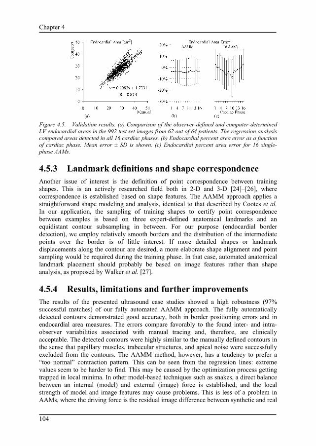
Chapter 4

104

Figure 4.5. Validation results. (a) Comparison of the observer-defined and computer-determined LV endocardial areas in the 992 test set images from 62 out of 64 patients. The regression analysis compared areas detected in all 16 cardiac phases. (b) Endocardial percent area error as a function of cardiac phase. Mean error ± SD is shown. (c) Endocardial percent area error for 16 single-phase AAMs.

4.5.3 Landmark definitions and shape correspondence Another issue of interest is the definition of point correspondence between training shapes. This is an actively researched field both in 2-D and 3-D [24]–[26], where correspondence is established based on shape features. The AAMM approach applies a straightforward shape modeling and analysis, identical to that described by Cootes et al. In our application, the sampling of training shapes to certify point correspondence between examples is based on three expert-defined anatomical landmarks and an equidistant contour subsampling in between. For our purpose (endocardial border detection), we employ relatively smooth borders and the distribution of the intermediate points over the border is of little interest. If more detailed shapes or landmark displacements along the contour are desired, a more elaborate shape alignment and point sampling would be required during the training phase. In that case, automated anatomical landmark placement should probably be based on image features rather than shape analysis, as proposed by Walker et al. [27].

4.5.4 Results, limitations and further improvements The results of the presented ultrasound case studies showed a high robustness (97% successful matches) of our fully automated AAMM approach. The fully automatically detected contours demonstrated good accuracy, both in border positioning errors and in endocardial area measures. The errors compare favorably to the found inter- and intra-observer variabilities associated with manual tracing and, therefore, are clinically acceptable. The detected contours were highly similar to the manually defined contours in the sense that papillary muscles, trabecular structures, and apical noise were successfully excluded from the contours. The AAMM method, however, has a tendency to prefer a “too normal” contraction pattern. This can be seen from the regression lines: extreme values seem to be harder to find. This may be caused by the optimization process getting trapped in local minima. In other model-based techniques such as snakes, a direct balance between an internal (model) and external (image) force is established, and the local strength of model and image features may cause problems. This is less of a problem in AAMs, where the driving force is the residual image difference between synthetic and real

Chapter 4

105

image, the content of which determines the size and direction of the update step in the parameter space. Variations in the gradient descent optimization method, multiple initializations, a multiresolution approach [18], hybrid AAM/ASM approach [19], or modeling other structures like epicardium, right ventricle, and valves may help to surpass local minima. Match results on the training data confirm that model initialization and/or lock-in range are candidates for improvement. Alternatively, if a very localized and precise detection is required, a combination with a local contour optimization (dynamic programming [1], snakes [10]) may be attempted.

For a practical application, we strive toward minimal user interaction to attain maximal automation and limit sources of variability. However, the user should always be allowed to apply additional corrections. AAMs allow a very elegant approach for interactive corrections, as recently described by Cootes and Taylor [28].

The described approach is not free of some limitations. As any AAM approach, its reliability depends on the range of variabilities covered in the training set. In case of clinical images, the patient set should include sufficient cases of expected pathologies. Also, images from different types of equipment or special imaging modes (use of contrast, harmonic imaging, etc.) may influence accuracy and may require training of specialized models. This is a topic of further investigation. Furthermore, the result is clearly limited by the quality and reproducibility of the training image and contour data: accurately validated borders on substantial data sets are required.

The temporal segmentation approach is fully automated for phase-normalized sequences, not requiring any operator interaction. Indicating the ED and ES frames for phase normalization, however, was not done automatically in this study, although ED images can be easily identified automatically using the ECG. It remains to be investigated whether good results can be achieved as well for sequences normalized on the ED frames only.

Segmentation of a 16-phase image sequence is fast with typical processing times of 6 s on an 800-MHz Windows PC. To our knowledge, no other fully automated approach has been reported yielding comparable results in a large clinical evaluation. Still, additional development is needed to include all standard views, all representative pathologies and determine the routine clinical performance in a large scale clinical study validation.

In this study we have shown that AAMMs can automatically detect endocardial contours practically equivalent to those defined by a human expert. We should note that the clinical quality of quantitative information derived from these contours remains to be determined. We expect the AAMM method to be useful for full-cycle LV volume measurements, locating and quantifying wall motion abnormalities, localizing ischemia, etc. Proving its clinical significance for such applications is beyond the scope of this paper and remains the subject of future clinical studies.

4.6 Conclusions An AAM for normalized time sequences (AAMM) has been developed that models time-continuous cardiac motion and image appearance and performs fast, robust, fully automated contour detection on phase-normalized cardiac time sequences in a practically applicable manner. It generates time-continuous segmentation results, which are consistent with cardiac dynamics. The AAMM demonstrated robustness and accuracy in a

Chapter 4

106

large clinical study of LV segmentation using four-chamber transthoracic ultrasound image sequences.

References [1] J. G. Bosch, G. van Burken, F. Nijland, and J. H. C. Reiber, "Overview of automated quantitation

techniques in 2D echocardiography," in What's new in cardiovascular imaging, J. H. C. Reiber and E. E. van der Wall, Eds. Dordrecht, the Netherlands: Kluwer, 1998, pp. 363–376.

[2] D. B. Sher, S. Revankar, and S. Rosenthal, "Computer methods in quantitation of cardiac wall parameters from two dimensional echocardiograms: a survey," Int. J. Card. Imaging, vol. 8, pp. 11–26, 1992.

[3] J. E. Perez, A. D. Waggoner, B. Barzilai, H. E. Melton, J. G. Miller, and B. E. Sobel, "On-line assessment of ventricular function by automatic boundary detection and ultrasonic backscatter imaging," J. Am. Coll. Cardiol., vol. 19, pp. 313–320, 1992.

[4] E. A. Geiser, D. C. Wilson, D. X. Wang, D. A. Conetta, J. D. Murphy, and A. D. Hutson, "Autonomous epicardial and endocardial boundary detection in echocardiographic short-axis images," J. Am. Soc. Echocardiogr., vol. 11, pp. 338–348, 1998.

[5] T. Brotherton, T. Pollard, P. Simpson, and A. DeMaria, "Echocardiogram structure and tissue classification using hierarchical fuzzy neural networks," in Proc. IEEE Conf. Acoustics, Speech and Signal Proc., New York: IEEE Computer Society Press, 1994, pp. 573–576.

[6] J. M. B. Dias and J. M. N. Leitao, "Wall position and thickness estimation from sequences of echocardiographic images," IEEE Trans. Med. Imag., vol. 15, pp. 25–38, 1996.

[7] T. Gustavsson, S. Molander, R. Pascher, Q. Liang, H. Broman, and K. Caidahl, "A model-based procedure for fully automated boundary detection and 3D reconstruction from 2D echocardiograms," in Proc. Computers in Cardiol., A. Murray, Ed. Los Alamitos, CA: IEEE Computer Society Press, 1994, pp. 209–212.

[8] N. Friedland and D. Adam, "Echocardiographic myocardial edge detection using an optimization protocol," in Proc. Computers in Cardiol., K. Ripley, Ed. Los Alamitos, CA: IEEE Computer Society Press, 1989, pp. 379–382.

[9] M. Belohlavek, A. Manduca, T. Behrenbeck, J. Seward, and J. F. Greenleaf, "Image analysis using modified self-organizing maps: automated delineation of the left ventricular cavity in serial echocardiograms," in Proc. Conf. Visualisation in Biomedical Computing '96, K. H. Hoehne and R. Kikinis, Eds. Berlin: Springer, 1996, pp. 247–252.

[10] V. Chalana, D. T. Linker, D. R. Haynor, and Y. Kim, "A multiple active contour model for cardiac boundary detection on echocardiographic sequences," IEEE Trans. Med. Imag., vol. 15, pp. 290–298, 1996.

[11] T. Hozumi, K. Yoshida, H. Yoshioka et al., "Echocardiographic estimation of left ventricular cavity area with a newly developed automated contour tracking method," J. Am. Soc. Echocardiogr., vol. 10, pp. 822–829, 1997.

[12] A. D. Parker, A. Hill, C. J. Taylor, T. F. Cootes, X. Y. Jin, and D. G. Gibson, "Application of point distribution models to the automated analysis of echocardiograms," in Proc. Computers in Cardiol., A. Murray, Ed. Los Alamitos, CA: IEEE Computer Society Press, 1994, pp. 25–28.

[13] T. F. Cootes, A. Hill, C. J. Taylor, and J. Haslam, "Use of active shape models for locating structures in medical images," Image and Vision Computing, vol. 12, pp. 355–366, 1994.

[14] J. Montagnat, H. Delingette, and G. Malandain, "Cylindrical echocardiographic image segmentation based on 3D deformable models," in Medical Image Computing and Computer Aided Intervention (MICCAI'99), C. Taylor and A. Colchester, Eds. LNCS vol. 1679, Springer, Berlin, pp. 168–175, 1999.

[15] E. D. Angelini, A. F. Laine, S. Takuma, J. W. Holmes, and S. Homma, "LV volume quantification via spatiotemporal analysis of real-time 3D echocardiography," IEEE Trans. Med. Imag. vol. 20, pp. 457–469, 2001.

[16] G. Jacob, J. A. Noble, M. Mulet-Parada, and A. Blake, "Evaluating a robust contour tracker on echocardiographic sequences," Medical Image Analysis, vol. 3, pp. 63–75, 1999.

[17] T. F. Cootes, G. J. Edwards, and C. J. Taylor, "Active Appearance Models," IEEE Trans. Pattern Anal. Machine Intell., vol. 23, pp. 681–685, 2001.

[18] T. F. Cootes and C. J. Taylor, "Statistical models of appearance for medical image analysis and computer vision," in Proc. SPIE Medical Imaging 2001, Image Processing, M. Sonka and K. Hanson, Eds. Bellingham, WA: SPIE, 2001, pp. 236–248.

Chapter 4

107

[19] S. C. Mitchell, B. P. F. Lelieveldt, R. J. van der Geest, H. G. Bosch, J. H. C. Reiber, and M. Sonka, "Multistage hybrid Active Appearance Model matching: segmentation of left and right ventricles in cardiac MR images," IEEE Trans. Med. Imag., vol. 20, pp. 415–423, 2001.

[20] H. G. Bosch, S. C. Mitchell, B. P. F. Lelieveldt, M. Sonka, F. Nijland, and J. H. C. Reiber, “Feasibility of fully automated border detection on stress echocardiograms by Active Appearance Models,” abstract, Circulation, vol. 102, p. II-633, 2000.

[21] C. Goodall, "Procrustes methods in the statistical analysis of shape," J. Royal Stat. Soc. B. vol. 53, pp. 285–339, 1991.

[22] E. P. Gordon, I. Schnittger, P. J. Fitzgerald, P. Williams, and R. L. Popp, "Reproducibility of left ventricular volumes by two-dimensional echocardiography," J. Am. Coll. Cardiol., vol. 2, pp. 506–513, 1983.

[23] T. F. Cootes, G. V. Wheeler, K. N. Walker, and C. J. Taylor, "Coupled-View Active Appearance Models," in Proc. British Machine Vision Conf. 2000, vol. 1, pp. 52–61, 2000.

[24] H. D. Tagare, "Shape-based nonrigid correspondence with application to heart motion analysis," IEEE Trans. Med. Imag. vol. 18, pp. 570–579, 1999.

[25] A. F. Frangi, D. Rueckert, J. A. Schnabel, and W. J. Niessen, "Automatic 3D ASM construction via atlas-based landmarking and volumetric elastic registration," in Proc. IPMI 2001, M. F. Insana and R. M. Leahy (Eds.), LNCS vol. 2082, Springer, Berlin, pp. 78–91, 2001.

[26] R. H. Davies, T. F. Cootes, and C. J. Taylor, "A minimum description length approach to statistical shape modelling," in Proc. IPMI 2001, M. F. Insana and R. M. Leahy (Eds.), LNCS vol. 2082, Springer, Berlin, pp. 50–63, 2001.

[27] K. N. Walker, T. F. Cootes, and C. J. Taylor, "Automatically building appearance models from image sequences using salient features," in Proc. British Machine Vision Conf. '99, T. Pridmore (Ed.), pp. 463–472, 1999.

[28] T. F. Cootes and C. J. Taylor, "Constrained Active Appearance Models," in Proc. Int. Conf. Computer Vision 2001. Vol. I. Los Alamitos, CA: IEEE Computer Society Press, 2001, pp. 748–754.

Chapter 4

108

109

Chapter 5

3-D Active Appearance Models: segmentation of cardiac MR and

ultrasound images.

Steven C. Mitchell1, Johan G. Bosch2, Boudewijn P.F. Lelieveldt2, Rob J. van der Geest2,

Johan H.C. Reiber2, Milan Sonka1.

1Department of Electrical and Computer Engineering, University of Iowa, Iowa City, IA, United States of America.

2Division of Image Processing, Department of Radiology,

Leiden University Medical Center, Leiden, The Netherlands.

IEEE Trans Med Imaging 21 (2002): 1167-1178.

Chapter 5

110

Abstract A model-based method for three-dimensional image segmentation was developed and its performance assessed in segmentation of volumetric cardiac magnetic resonance (MR) images and echocardiographic temporal image sequences. Comprehensive design of a three-dimensional (3-D) active appearance model (AAM) is reported for the first time as an involved extension of the AAM framework introduced by Cootes et al. The model’s behavior is learned from manually traced segmentation examples during an automated training stage. Information about shape and image appearance of the cardiac structures is contained in a single model. This ensures a spatially and/or temporally consistent segmentation of three-dimensional cardiac images.

The clinical potential of the 3-D AAM is demonstrated in short-axis cardiac MR images and four-chamber echocardiographic sequences. The method’s performance was assessed by comparison with manually identified independent standards in 56 clinical MR and 64 clinical echo image sequences. The AAM method showed good agreement with the independent standard using quantitative indices of border positioning errors, endo- and epicardial volumes, and left ventricular mass. In MR, the endocardial volumes, epicardial volumes, and left ventricular wall mass correlation coefficients between manual and AAM were R2 = 0.94, 0.97, 0.82 respectively. For echocardiographic analysis, the area correlation was R2 = 0.79. The AAM method shows high promise for successful application to MR and echocardiographic image analysis in a clinical setting.

Chapter 5

111

5.1 Introduction Cardiovascular disease is the number one cause of death in the Western world. Cardiac imaging is an established approach to diagnosing cardiovascular disease and plays an important role in its interventional treatment. Three-dimensional (3-D) imaging of the heart and the cardiovascular system is now possible with X-ray computed tomography, magnetic resonance (MR), positron emission tomography, single photon emission tomography, and ultrasound, to name just the main imaging modalities. While cardiac imaging capabilities are developing rapidly, the images are mostly analyzed visually, and therefore qualitatively. The ability to quantitatively analyze the acquired image data is still not sufficiently available in routine clinical care. Large amounts of acquired data are not fully utilized because of the tedious and time-consuming character of manual analyses. This is even more so when three-dimensional image data need to be processed and analyzed. Image segmentation is a prerequisite to quantitative analysis, and thus developing methods for highly automated three-dimensional cardiac image segmentation is of primary importance.

There are three main reasons why existing methods frequently exhibit lower the success rate in comparison with human expert observers, especially when applied to clinical-quality images: existing methods do not incorporate a sufficient amount of a priori knowledge about the segmentation problem; do not consider three-dimensional or temporal context as an integral part of their functionality; and position the segmentation boundaries at locations of the strongest local image features not considering true anatomical boundary locations.

A number of 3-D medical image analysis approaches have occurred recently, many of them addressing one or more of the above-mentioned shortcomings of available segmentation techniques. A detailed review of existing 3-D cardiac modeling approaches is provided in [1]. In the context of our work and considering the goal of segmenting three-dimensional volumetric and temporal cardiac images and image sequences, statistical modeling of 3-D shape and 3-D image properties is crucial. Vemuri et al. concentrated on a 3-D model that combines deformed superquadric primitives with a local displacement field expressed on an orthonormal wavelet basis [2]. As a result of this orthonormal basis, the shape parameters become physically meaningful, and thus a preferred shape can be imposed based on parameter distributions in a set of training samples. Similarly, Staib et al. developed a three-dimensional balloon model [3].The model is parameterized on an orthonormal Fourier basis such that the statistics of the Fourier coefficients in a training set allow a constrained image search. Model fitting in these two methods is performed by balancing an internal energy term with an external, gradient-derived scalar field.

Cootes and Taylor developed a statistical point distribution model (PDM) and demonstrated its utility for two-dimensional (2-D) image segmentation [4], [5]. One of the primary contributions was an ease of automated learning of the model parameters from sets of corresponding points as well as the PDM’s ability to incorporate shape and boundary gray-level properties and their allowed variations. Applications to segmentation of echocardiographic data [6] and deep neuroanatomical structures from MR images of the brain may serve as examples [7]. Following the point distribution model ideas,

Chapter 5

112

Kelemen et al. built a statistical model of three-dimensional shapes using parametric surface representations [8]. Similar to PDMs, shape and gray-level information in the boundary vicinity was incorporated in the model. The method’s performance was demonstrated on 3-D segmentation of neuroanatomical structures. A multiscale 3-D shape modeling approach called M-reps was developed by Pizer et al. [9]. M-reps support a coarse-to-fine hierarchy and model shape variations via probabilistically described boundary positions with width- and scale-proportional tolerances. Three-dimensional echocardiographic image segmentation using core atoms was reported by Stetten [10]. Davatzikos et al. presented a deformable model in which geometric information is embedded via a set of affine-invariant attribute vectors; these vectors characterize the geometric structure around a model point from a local to a global scale, forming an adaptive focus deformable statistical shape model [11]. The methodology was applied to segmentation of neuroanatomical structures.

In all the above-referenced approaches, the models primarily hold information about shape and its allowed variations. The information about image appearance is only considered in close proximity to the object borders. A powerful, model-driven segmentation technique called active appearance model (AAM) was recently introduced by Cootes et al. [12]–[14]. An AAM describes the image appearance and the shape of an object in a set of examples as a statistical shape-appearance model. AAMs can be applied to image segmentation by minimizing the difference between the model and an image along statistically plausible shape/intensity variations (analysis by synthesis). AAMs have shown to be highly robust in the segmentation of routinely acquired single-phase single-slice cardiac MR [15] and echo images [16], because they exploit prior knowledge about the cardiac shape, image appearance, and observer preference in a generic way. For a detailed background on AAMs and their application to image segmentation, the reader is referred to [13].

Until now, AAMs have only been applied to 2-D images and to normalized (fixed-phase) 2-D time sequences [15]–[17]. Two-dimensional active appearance motion models [16], [17] have demonstrated the ability of time-continuous segmentation by exploiting temporal coherency in the data. However, these 2-D + time AAMs do not represent a true 3-D approach. Their segmentation ability is limited to cases with fixed numbers of preselected frames; they rely on a priori knowledge of image frame correspondences within each cardiac cycle.

The primary contribution of this paper is the development of a fully three-dimensional active appearance model (3-D AAM) that requires no additional interactively supplied information. A demonstration of its segmentation performance in volumetric or temporal image segmentation of cardiac structures is given below. No 3-D AAM has been reported to date that is capable of successful segmentation of cardiac MR and echocardiographic images. The model’s behavior is learned from manually traced segmentation examples during an automated training stage. The shape and image appearance of the cardiac structures are contained in a single model. This ensures a spatially and/or temporally consistent segmentation of three-dimensional cardiac images.

Chapter 5

113

5.2 Methods 5.2.1 Point distribution model concept Point distribution models describe populations of shapes using statistics of sets of corresponding landmarks of the shape instances [4], [5], [18]. By aligning N shape samples (consisting of n landmark points) and applying a principal component analysis (PCA) on the sample distribution, any sample x within the distribution can be expressed as an average shape x with a linear combination of eigenvectors P superimposed

Pbxx += (5.1)

In two-dimensional models, p = min(2n, N-1) eigenvectors P form the principal basis functions, while in a three-dimensional model, p = min(3n, N-1) eigenvectors are formed. (The minimum operator is needed since we frequently have more corresponding shape points than training set samples.) In both cases, the corresponding eigenvalues provide a measure for compactness of the distribution along each axis. By selecting the largest q eigenvalues, the number of eigenvectors can be reduced, where a proportion k of the total variance is described such that

∑∑==

=⋅≥p

ii

q

ii TotalwhereTotalk

11λλ (5.2)

5.2.2 Representing shape of 3-D cardiac ventricles Extending the two-dimensional PDM to three dimensions is a nontrivial task. To create a compact and specific model, point correspondences between shapes are required. Even if landmark points are easily identifiable in both models, specifying uniquely corresponding boundary points in between these landmarks is difficult in 3-D. In a 2-D case [15], boundary points may be identified by evenly sampling points on a boundary from one landmark to the next. In a 3-D case, the problem lies in defining a unique sampling of the object surfaces.

For the purpose of ventricular segmentation, a normalized cylindrical coordinate system is defined with its primary axis aligned with the long axis of the heart and the secondary axis aligned with the posterior junction of the right and left ventricles in the basal slice. The cardiac ventricles resemble a cylindrical or paraboloid shape. First, contours are sampled slice-by-slice at even angle increments. To transform the rings in the normalized cylindrical coordinate system, each point on the ring is connected by a straight line to the next adjacent corresponding point on the rings above and below. Starting from the apex slice to the basal slice, a fixed number of slicing planes are placed evenly along the long axis. New points are interpolated where the planes intersect the lines. This yields a set of corresponding boundary points for each sampled left ventricle across the population of ventricles (Fig. 5.1).

Chapter 5

114

Figure 5.1. A cross-sectional depiction of trans- Figure 5.2. A wireframe representation forming a cardiac MR stack with manually placed of the mean LV shape in the normalized landmarks to a normalized cylindrical coordinate cylindrical coordinate system. system.

5.2.3 Three-dimensional point distribution models Aligning shape samples to a common scale, rotation, and translation is important for a compact model to be generated during the PCA stage. Procrustes analysis [19], [20] is used, whereby an arbitrary shape is selected as the initial average shape estimate. All the other shapes are aligned to this average using a least squares minimization. A new average is computed by a simple mean across the corresponding points, and the algorithm repeats until convergence.

For the 2-D case, aligning one shape to another can be solved analytically by minimizing scale, rotation, and translation terms. Extending to 3-D, the minimization of scaling, translations, and rotation differences along the three axes may lead to singularities known as gimbal lock. Assuming that 3-D translation is represented by a separate translation vector t, a quaternion q representation of scaling and rotation avoids such behavior [21].

A quaternion q is defined as the linear combination of a scalar term q0 ≥ 0 and three right-handed orthonormal vectors (i, j, and k) q = q0 + q1 i + q2 j + q3 k. (5.3) The magnitude of the quaternion is defined as

23

22

21

20 qqqq +++=q (5.4)

and any unit length quaternion can be written as q = cos(ϕ )⋅u + sin(ϕ )⋅u (5.5) where u is a unit vector and ϕ represents a rotational twist along the unit vector. Thus, any scaling and rotation in 3-D can be expressed as a quaternion, where scaling is expressed by the magnitude of the quaternion and the 3-D rotation is expressed by the direction of the unit vector u and rotation ϕ.

Chapter 5

115

The Cartesian rotation matrix is shown in (5.6)

( ) ( )( ) ( )( ) ( ) ⎥

⎥⎥

⎦

⎤

⎢⎢⎢

⎣

⎡

−−++−−−−+++−−−+

=22

21

23

2010322031

103223

21

22

203021

2031302123

22

21

20

222222

qqqqqqqqqqqqqqqqqqqqqqqqqqqqqqqqqqqq

R (5.6)

Together, the position and orientation of a 3-D object can be represented as a seven-element pose vector: ( ) [ ]kji tttqqqq ,,,,,, 3210=tq . The alignment of two 3-D shape instances is accomplished using a well-known procedure given by Besl et al. [22] to optimize for q and t. Aligning all the shapes is a matter of employing the Procrustes analysis using Besl’s procedure to calculate the pose parameters. Once shape alignment is finished, principal component analysis is applied to the 3-D models in a way that is no different from the conventional 2-D application [5].

5.2.4 Modeling volume appearance The first part of creating an appearance model of volume is to warp all the sample volumes to the average shape to eliminate shape variation and bring voxel-wise correspondence across all the training samples, such that the voxel intensities can be represented as a shape-free vector of intensity values. Warping an image I to a new image I’ involves creating a function that maps control points xi to xi’ as well as the intermediate points in between. For the 2-D case, either piecewise affine warping or thin-plate spline warping is adequate. In our models, piecewise warping is preferred because it is significantly faster than thin-plate spline warping.

In 2-D piecewise affine warping, landmark points are used to construct the shape area as a set of triangles. The well-known Delaunay triangulation algorithm is suitable for computing such a triangular mesh and can be found in many computational geometry references. Individual triangular patches are locally warped using barycentric coordinates. Given a triangle with the three corners x1, x2, and x3, we can represent any point x within the triangle as x = αx1 + βx2 + γx3, where γ = 1 – (α + β) or α + β + γ = 1. In order for a point x to fall inside a triangle, 0 ≤ α, β, γ ≤ 1 must be true.

Piecewise affine warping is implemented as follows. For each pixel location x’ in I’:

1. Find the triangle t’ that contains x’ by solving α, β, and γ for each triangle and finding the triangle where 0 ≤ α, β, γ ≤ 1.

2. Find the equivalent pixel location x by computing x = αx1 + βx2 + γx3, where x1, x2, and x3 are the triangle points from the original image.

3. Copy the pixel value in I located by x into the warped image I’ located at x’. Some form of pixel interpolation such as bilinear may be used at this stage.

In our 3-D models, piecewise affine warping is extended to tetrahedrons with four corners x1, x2, x3, and x4. Any point within the tetrahedron is represented as x = αx1 + βx2 + γx3 + δx4. In a general case, creating a tetrahedral representation of volume is solved using a 3-D Delaunay triangulation algorithm. However, due to the cylindrical nature of the left

Chapter 5

116

ventricular (LV) shape, a manually defined volume partitioning in regular tetrahedrons was utilized. Each slice level is constructed of pie-shaped wedges built on four tetrahedrons with exterior profile cubes built with five tetrahedrons. Piecewise affine warping is implemented in a similar fashion as in the 2-D case. Because all volumes are warped to the average volume, barycentric coordinates α, β, γ, δ are precomputed for each fixed voxel point, eliminating the time-consuming process of searching for the enclosing tetrahedron for each voxel point during the matching. Due to the regular geometry of the tetrahedrons in our volume partitioning, the barycentric coordinate computation did not become ill-posed.

After the warping phase, the shape-free intensity vectors are normalized to an average intensity of zero and an average variance of one to remove the effects of brightness and contrast variations across scans. Next, PCA is applied to the shape-free intensity vectors to create an intensity model. In agreement with the AAM principle, shape information and intensity information are combined into a single active appearance model. Lastly, another PCA is applied to the coefficients of the shape and intensity models to form a combined appearance model [23].

In the equations below, the subscript s corresponds to shape parameters and the subscript g represents intensity (gray-level) parameters. To summarize, the 3-D AAM is created as follows.

1) Let xi denote a vector of 3-D landmark points for a given sample i. Compute a 3-D PDM and approximate each shape sample as a linear combination of eigenvectors, where ( )xxPb −= T

ss represents the sample shape parameters. 2) Warp each image to the mean shape using a warping such as piecewise affine

or thin plate spline warping to create shape-free intensity vectors. 3) Normalize each intensity vector, applying a global intensity transform with

parameters hi , to match the average intensity vector g . 4) Perform a PCA on the normalized intensity images. 5) Express each intensity sample as a linear combination of eigenvectors, where

( )ggPb −= Tgg represents the sample shape parameters.

6) Concatenate the shape vectors bs and gray-level intensity vectors bg in the following manner:

( )

( ) ⎟⎟⎠

⎞⎜⎜⎝

⎛

−−

=⎟⎟⎠

⎞⎜⎜⎝

⎛=

ggPxxWP

bWb

b Tg

Ts

g

s (5.7)

where the weighting matrix W is a diagonal matrix relating the different units

of shape and intensity coefficients. 7) Apply a PCA to the sample set of all b vectors, yielding the appearance model

b = Qc. (5.8)

5.2.5 Matching 3-D AAM to image data Matching an appearance model to image data involves minimizing the root mean square (rms) intensity difference between the image data and appearance model instance by

Chapter 5

117

modifying the affine transformation, global intensity parameters, and appearance coefficients. A gradient descent method is used that employs the relation between model coefficient changes and changes in the voxel intensity difference between the target image and synthesized model [23]. This relation is derived during a training stage.

Let t and q represent the translation and quaternion transformation parameters and h the intensity transform parameters. As shown above, shape x is derived in the target image from the appearance coefficient c and the affine transformation vectors t and q. Then, shape intensity vector gs is sampled from the target volume data after warping the space defined by x to the mean shape x . The model intensity vector gm is derived from the appearance coefficients c with the global intensity corrected via h. The error function E is the rms difference of gs - gm.

Gradient descent optimization requires the partial derivatives of the error function defined by the intensity of the target and synthesized model volume. While it is not possible to create such a function analytically, these derivatives may be approximated using fixed matrices computed by randomly perturbing model coefficients for a set of known training images and observing the resulting difference in error images [23]. Using a set of training images, their corresponding modeling parameters c, t, q, and h are randomly displaced, thus creating a difference between gs and gm. From the parameter displacements and the resulting difference intensity vectors, gradient approximating matrices Ac, At, Aq, and Ah can be determined using reduced-rank multivariate linear regression. Alternatively, the gradient matrices may be built one column at a time by averaging the Gaussian weighted differences between the target and synthesized image of each individual model perturbation. The latter method is preferred for 3-D AAM matching due to lower memory requirements, better representation of high order eigenmodes, and faster computation. This iterative refinement technique of precomputed fixed matrices versus brute-force gradient descent optimization was formulated by Cootes [13] as well as by Baker and Matthews [24]. Formally, the gradient matrices are created as follows.

1) Select an object from the training set with known appearance model parameters c0, t0, q0, and h0.

2) For each element in the model parameters, c, t, q, or h, perturb a single element by a fixed δp with the rest of δc, δt, δq, and δh assigned to zero. Typically, c is perturbed within ±1.5 standard deviation, t by 3–5 voxels, and q, h by 10% of their original value.

3) Let c = δc + c0. Compute shape x and texture gm. 4) Apply an affine transformation to x by first transforming x using δt and δq,

then transforming the result by t0 and q0. This cascaded transform is required to maintain linearity.

5) Create the image patch gs warped from the target image to the mean shape using shape x.

6) Apply global intensity scaling to gs by using δh first and then scaling the result by h0.

7) Compute δg = gs - gm. 8) Compute the slope, δs = δg / δp. Weight the slope by a normalized Gaussian

function with the ±3 standard deviation set to the maximum and minimum model perturbation values.

9) Accumulate the slope with previous slopes for that given element.

Chapter 5

118

10) Go to Step 2) and repeat until all elements and perturbations of each element are sufficiently covered. Place the average slope into the appropriate column in the gradient matrices Ac, At, Aq, or Ah.

11) Go to Step 1) and repeat until there is sufficient coverage of displacement vectors.

The corresponding model correction steps are computed as δc = Ac (gs - gm) (5.9) δt = At (gs - gm) (5.10) δq = Aq (gs - gm) (5.11) δh = Ah (gs - gm) (5.12) Matching the AAM to the image data is accomplished as follows.

1) Place the mean appearance model (c, h = 0; t, q defined by the initial model position) roughly on the object of interest and compute the difference image gs - gm.

2) Compute the rms error of the difference image E. 3) Compute the model corrections δc, δt, δq, and δh from the difference image

[(5.9)–(5.12)]. 4) Set k = 1. 5) Compute new model parameters as c := c - kδc, t := t - kδt, q := q - kδq, and

h := h - kδh. 6) Based on these new parameters, recompute gs - gm and find the rms error. 7) If the rms error is less than E go to Step 2). 8) Else try setting k to 1.5, 0.5, 0.25, 0.125, etc., and go to Step 5. Repeat steps 5–

8 until the error cannot be reduced any further.

5.3 Case studies To investigate the clinical potential of the reported 3-D active appearance model under clinically realistic conditions, AAMs were trained and tested in two substantially different medical imaging modalities: multislice short-axis cardiac magnetic resonance and four-chamber echocardiographic image sequences. While the overall approach is identical in the two reported application areas, some modality- as well as application-specific differences exist and are provided as follows.

5.3.1 Cardiac MRI

5.3.1.1 Data Cardiac MR image sequences were collected from 38 normal subjects and 18 patients, yielding a total of 56 short-axis 3-D cardiac MR data sets. Patients were selected who were suffering from different common cardiac pathologies (among others, different types of myocardial infarction, hypertrophic cardiomyopathy, arrhythmia). Images were acquired using standard electrocardiography (ECG) gated fast field echo MR pulse sequences on a Philips Gyroscan NT 15 scanner. Slices were acquired in a per-slice manner, under breathhold in end-expiration. End-diastolic images were used in this study.

Chapter 5

119

Image resolution was 256 × 256 pixels, with a field of view of 400–450 mm and slice thickness of 8–11 mm. Between eight and 14 slices were scanned to at least cover the entire left ventricle, depending on LV dimensions and slice spacing.

5.3.1.2 Independent Standard The left ventricular endocardium and epicardium were manually traced by an expert observer who was blinded to the results of the computer analysis. Following common practice in clinical quantitative cardiac MR analysis, endocardial (ENDO) contours were drawn behind the papillary muscles and trabeculae, and epicardial (EPI) contours were drawn on the inside of the epicardial fat layer. The apical slice was defined as the last slice with both ENDO and EPI contours visible. Apex slices with merely a small visible muscle cap were excluded. In each slice, a reference point was manually placed at the posterior junction of the left and right ventricular walls to define point correspondence between different samples as required during the AAM training.

5.3.1.3 Training using leave-one-out approach To maximize the effective size of the training set, validation was performed using a leave-one-out approach [25]. AAM models were trained on image and contour data from 55 subjects, and the model matching performance was subsequently evaluated on the one left-out data set. The training process was repeated 56 times, always leaving out a different data set, which was then used for validation. The model voxel size varied from one data set to another, but in general with 3 × subsampling, the model occupied approximately 6000 voxels and required about 1 h of training and 2–3 min for matching on a 1-GHz Windows PC.

5.3.1.4 Matching procedure In midventricular short-axis MR images, the left ventricle can usually be identified as an approximately circular object (Fig. 5.3(a)). This fact is used for automated initialization of the 3-D AAM. A previously validated Hough transform-based method determines a 2-D centroid of the LV long axis for each MR image slice [26]. A 3-D centroid of a line segment fitted through the 2-D centroids of individual MR slices defines the initial position of the 3-D AAM.

To make the 3-D segmentation procedure completely independent from any user interaction regarding the rotation and scale of the heart in the short-axis plane, the matching process was repeatedly performed for a range of five orientations and three scales. This multiple initialization is important because AAM matching may be dependent on initial positioning since gradient descent may contain local minima. The matching result yielding the smallest quadratic intensity error was selected as the final match. The matching procedure resulted in a set of endo-and epicardial contours for each volumetric MR image.

5.3.1.5 Quantitative validation To exclude obvious matching errors from further quantitative analyses, matching results were visually evaluated. A matching result was scored as acceptable when the ENDO and EPI contours in the majority of slices showed good agreement with the image data. The number of unacceptable results yielding matching failures is reported. Studies with a

Chapter 5

120

(a) (b) Figure 5.3. Example cardiac MR images used for validation. (a) LV segmentation was performed in volumetric images consisting of 8–12 full-size MR images like the one shown here. (b) Subimages depicting LV detail in all nine images of this volumetric data set. See Fig. 5.4 for the segmentation results. poorly localized apex but with correctly localized mid-ventricular segments were graded as acceptable. In some cases, the 3-D model did not deploy far enough to span over all the slices for which manual contours were available. Then, manual contours were present in extreme apical or basal slices but no automatic contours were identified there. Such segmentations were not excluded, and the numbers of slices missed by the AAM method are reported below.

To quantitatively assess the performance of the 3-D AAM approach, surface positioning errors were determined comparing the automatically detected endo- and epicardial surfaces with the independent standard. The average signed and unsigned surface positioning errors were defined by measuring the distances between points along rays perpendicular to the centerline between the respective manual contours and the computer-determined surfaces; 100 rays were used for each contour. Surface positioning errors are expressed in millimeters as mean ± standard deviation. A negative sign of the signed error value means that the automatically determined surface was inside of the observer-defined surface.

Three clinically important measures were calculated and used for performance assessment: LV cavity volume, LV epicardial volume, and LV myocardial mass. The volumetric indexes were determined using all slices for which both manually traced contours and computer-determined surfaces were available and were expressed in cm3. The LV mass measurements are reported in g. Regression analysis was used to compare the computer measurements with the independent standard.

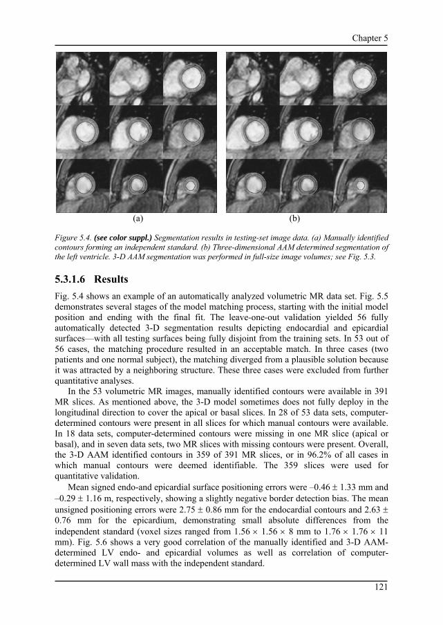
Chapter 5

121

(a) (b) Figure 5.4. (see color suppl.) Segmentation results in testing-set image data. (a) Manually identified contours forming an independent standard. (b) Three-dimensional AAM determined segmentation of the left ventricle. 3-D AAM segmentation was performed in full-size image volumes; see Fig. 5.3.

5.3.1.6 Results Fig. 5.4 shows an example of an automatically analyzed volumetric MR data set. Fig. 5.5 demonstrates several stages of the model matching process, starting with the initial model position and ending with the final fit. The leave-one-out validation yielded 56 fully automatically detected 3-D segmentation results depicting endocardial and epicardial surfaces—with all testing surfaces being fully disjoint from the training sets. In 53 out of 56 cases, the matching procedure resulted in an acceptable match. In three cases (two patients and one normal subject), the matching diverged from a plausible solution because it was attracted by a neighboring structure. These three cases were excluded from further quantitative analyses.

In the 53 volumetric MR images, manually identified contours were available in 391 MR slices. As mentioned above, the 3-D model sometimes does not fully deploy in the longitudinal direction to cover the apical or basal slices. In 28 of 53 data sets, computer-determined contours were present in all slices for which manual contours were available. In 18 data sets, computer-determined contours were missing in one MR slice (apical or basal), and in seven data sets, two MR slices with missing contours were present. Overall, the 3-D AAM identified contours in 359 of 391 MR slices, or in 96.2% of all cases in which manual contours were deemed identifiable. The 359 slices were used for quantitative validation.

Mean signed endo-and epicardial surface positioning errors were –0.46 ± 1.33 mm and –0.29 ± 1.16 m, respectively, showing a slightly negative border detection bias. The mean unsigned positioning errors were 2.75 ± 0.86 mm for the endocardial contours and 2.63 ± 0.76 mm for the epicardium, demonstrating small absolute differences from the independent standard (voxel sizes ranged from 1.56 × 1.56 × 8 mm to 1.76 × 1.76 × 11 mm). Fig. 5.6 shows a very good correlation of the manually identified and 3-D AAM-determined LV endo- and epicardial volumes as well as correlation of computer-determined LV wall mass with the independent standard.

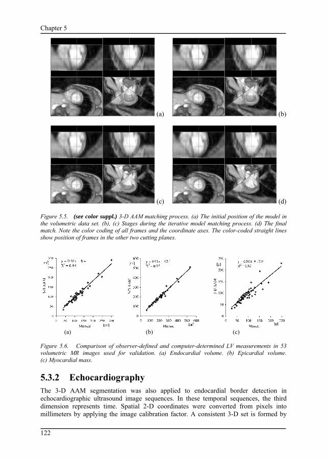
Chapter 5

122

(a) (b)

(c) (d) Figure 5.5. (see color suppl.) 3-D AAM matching process. (a) The initial position of the model in the volumetric data set. (b), (c) Stages during the iterative model matching process. (d) The final match. Note the color coding of all frames and the coordinate axes. The color-coded straight lines show position of frames in the other two cutting planes.

(a) (b) (c) Figure 5.6. Comparison of observer-defined and computer-determined LV measurements in 53 volumetric MR images used for validation. (a) Endocardial volume. (b) Epicardial volume. (c) Myocardial mass.

5.3.2 Echocardiography The 3-D AAM segmentation was also applied to endocardial border detection in echocardiographic ultrasound image sequences. In these temporal sequences, the third dimension represents time. Spatial 2-D coordinates were converted from pixels into millimeters by applying the image calibration factor. A consistent 3-D set is formed by

Chapter 5

123

converting the time dimension (s) into a spatial dimension (mm) using a fixed ratio (“speed” of 40 mm/s). This ratio was chosen to obtain similar sizes of the 3-D object in all three dimensions. A consistent 3-D voxel space is obtained in which the shape and appearance of the heart over a full cardiac cycle can be modeled as a 3-D object. A 3-D AAM for this object was applied to image sequences extending over three cardiac cycles. This approach allows fully automated detection of time-continuous contours in time sequences of arbitrary length without knowledge of end-diastolic (ED) and end-systolic (ES) time points. The model adjusts itself in both time and space and locates a complete cardiac cycle automatically. This is an important difference from the previously reported 2-D + time AAM approach [16].

In a training set, corresponding shape points on the endocardial contour are defined for each frame of one complete cardiac cycle (ED to ED) based on expert-drawn contours. Point correspondence in the third (time) dimension is defined by using the relative cardiac phase of each image. The relative cardiac phase of each image is modeled as a value between zero and two, defined for systolic frames as the frame’s relative position between ED and ES (range 0–1) and for diastolic frames as its relative position between ES and following ED incremented by one (range 1–2). For each training case, 17 time slices with equidistant relative phase (starting and ending with ED) are identified by nearest neighbor interpolation. Of these frames, the 2-D shape point coordinates are extended to 3-D spatial coordinates by multiplying the frame’s time by the speed ratio. The resulting 3-D shape is represented as a surface of 3-D points (Fig. 5.7). The image appearance of the heart is modeled as a vector of voxel intensity values in an image volume patch spanned by the manual contour surface, extended equally in all directions. Partitioning of the image volume into regular tetrahedrons was coded specifically for this shape. The actual image volume was sampled sparsely (factor 5–7) after appropriate Gaussian filtering to limit the dimension of the intensity vector to a practical size of a few thousand voxels. The 3-D AAM provides time-continuous segmentation for one complete cardiac cycle, located automatically in both time and space. An ultrasound-specific initialization procedure was followed, in which the model was allowed to iterate from 25 different initializations (five 3-D size factors ranging between 0.9 and 1.3 compared to the average size and five temporal positions along the time axis). The matching result with the lowest quadratic intensity error was considered the best match.

Data To allow comparison of 3-D AAM results with the 2-D + time AAM approach, the method was tested on the same data set [16]. Sets of transthoracic echocardiographic four-chamber sequences were acquired at 25 frames/s from 129 unselected infarct patients participating in a clinical trial. These were single-beat (end-diastole to end-diastole) sequences with 15–33 image frames per heartbeat artificially extended to three cardiac cycles as described above. Images were digitized at a resolution of 768 × 576 pixels with different calibration factors (0.28 to 0.47 mm/pixel). The total data set was split randomly into a training set of 65 patients and a testing set of 64 patients. The model voxel size varied from one data set to another, but in general with 8 × subsampling the model occupied approximately 7000 voxels, required about 1 h of training and 2–3 min for matching on a 1-GHz Windows PC. The larger subsampling of the echocardiographic model reduced the voxel size and complexity to approximately the same as the MR model, resulting in similar training and matching times.

Chapter 5

124

Figure 5.7. Motion of the left ventricular endocardium in ultrasound four-chamber cross section represented as a 3-D object. Time axis from bottom left to top right.

5.3.2.2 Independent standard In all sequences, an expert observer who was blinded to the computer analysis results manually outlined the contours of the endocardium in all frames of the image sequences. To compare the performance of 3-D AAMs with that of human experts, inter- and intra-observer variabilities of manual contour tracing were determined in a subset of 19 randomly chosen image sequences. Manual contour definition was independently repeated by the same expert observer and by another expert observer.

5.3.2.3 Quantitative validation To compare the automatically detected contours with the observer-identified independent standard, the number of segmentation failures was determined. Failures were identified as segmentations in which the 3-D AAM-defined borders did not agree well with the independent standard (average unsigned spatial distance component >7.5 mm). In the successfully segmented images, unsigned three-dimensional endocardial border positioning errors were defined as unsigned distances between matched model points and image-based 3-D shape points extracted for the testing-set images in a same manner as the training-set shape points. These distances were calculated in 3-D and also split into spatial (x,y) and temporal (z) components, where the temporal component can be expressed in mm or milliseconds by inverting the “speed” conversion specified above. Furthermore, endocardial areas were determined for all time slices; regression analysis was used to compare the computer-determined areas with the independent standard.

5.3.2.4 Results In 57 of the 64 tested echocardiographic image sequences (success rate 89%), the 3-D AAM-defined borders agreed well with the independent standard. An example of the

Chapter 5

125

Figure 5.8. (see color suppl.) Example of the 3-D AAM matching process in an ultrasound time sequence. The position of the model within the 3-D image data is shown in red. The independent standard is shown in green. Top row gives the initial positioning of the 3-D AAM; bottom row provides its final match. The left three panels represent image information along three perpendicular planes cutting through the three-dimensional data set. The leftmost column provides an image within the temporal plane; the two middle columns depict image data along the horizontal and vertical cutting planes. Note the color-coding of all frames and the coordinate axes. The color-coded straight lines show position of this frame in the other two cutting planes. In the rightmost panel, a 3-D rendering of model and independent standard is shown. matching procedure is given in Fig. 5.8. In the successful 57 temporal sequences, three-dimensional absolute endocardial surface positioning errors were 3.90 ± 1.38 mm; the 2-D spatial component was 3.35 ± 1.05 mm, which compares favorably with two-dimensionally determined (within the same image frame) inter-observer variability of 3.82 ± 1.44 mm. The intra-observer variability was 2.32 ± 0.75 mm. The result also compares reasonably well with the previously reported two-dimensional endocardial border positioning errors of 3.35 ± 1.22 mm (success rate 97%) achieved by our less general 2-D + time active appearance motion model implementation [16]. The temporal error of border positioning was 37.0 ± 29.6 ms, less than a single frame duration of 40 ms. Frame-based endocardial area regression over the 57 successful matches is given in Fig. 5.9.

5.4 Discussion A method for three-dimensional segmentation of medical images has been presented and its performance demonstrated in two cardiac image analysis applications. The method allows fully automated segmentation of volumetric or temporal images. Its inherent 3-D character incorporates information context in all three dimensions—a feature frequently not possible with previous approaches. The step leading from existing 2-D active appearance models to a functional 3-D AAM is not an easy one. Mastering the fully 3-D behavior will facilitate the method’s extension to analysis of three-dimensional temporal sequences, one of the ultimate goals of medical image analysis. This discussion will focus on three areas: 1) performance of the current method; 2) its limitations with respect to

Chapter 5

126

Figure 5.9. Comparison of observer-defined and computer-determined LV endocardial areas in all time slices of the 57 echocardiographic four-chamber sequences (969 images) used for validation. design of 3-D AAMs for clinical applications; and 3) future extensions of the methodology to facilitate four-dimensional image analysis.

5.4.1 Performance of the current method The described method is fully automated, with no user interaction. This is a significant strength in comparison to existing semiautomated approaches to cardiac segmentation that require almost undivided attention of the analysis operator. In addition, the value of the matching function after the 3-D AAM’s convergence can identify the situation when the model failed to segment the cardiac structures successfully, thus potentially allowing to incorporate yet another level of automated quality control. Consequently, it should be possible to identify segmentation successes with high confidence and then limit review of the results to a small number of image data sets for which the possibility of imperfect segmentation is indicated.

At present, performance robustness is achieved by multiple initializations; 15 initial positions of the model were used for MR segmentation and 25 different initializations for echocardiographic data. This approach improves the results but also increases computational demands. While the processing times are quite favorable—between 2–3 min for one data set in both applications (this includes the multiple initializations; 1-GHz Windows PC)—the number of model matching processes can be decreased by replacing brute-force multiple initializations with better positioning of the model. For example, information about the ventricular size and orientation is available in MR data from the Hough transform steps. In ultrasound, an estimate of ED and ES frames can be derived from ECG information or image sequence analysis, and there are several methods for estimating the size and position of ventricles automatically. No such information is currently utilized.

The border positioning errors as well as the volume and mass measures revealed a slight but systematic bias toward smaller contours. The presented 3-D AAM assumes the

Chapter 5

127

image data to be truly three-dimensional. However, the MR data sets are acquired over several heartbeats as sequences of 2-D slices, not in a volumetric fashion. Individual slices are frequently acquired during separate breath-holds. Differences in inspiration level and thus heart position lead to variable shifts in the LV position between slices. The effect of these shifts is threefold.

1) During the training of the model, unsystematic shifts are modeled in the shape model, decreasing the sensitivity of the model with respect to real shape variation.

2) During the matching, the match for multiple other adjacent slices is greatly disturbed by a single shifted slice.

3) The border positioning and volumetric errors are affected by the shifted slices. This may well explain a large part of the underestimation of the reported MR volume measures.

For the ultrasound application, results were promising but less convincing than those achieved using our previously reported 2-D + time AAM approach. Area regression (Fig. 5.9) over the 57 successful matches exhibited a systematic area underestimation of 3.8% (y = 0.83x + 3.6, R2 = 0.79). Compared to the 2-D + time AAM (y = 0.91x + 1.73, R2 = 0.76; area underestimation 2.9%), a slightly higher systematic area error and a flatter regression line were observed. In part, this can be attributed to the extra degree of freedom with which the 3-D AAM has to cope. The 2-D + time AAM uses a priori knowledge of the phase/time aspect. However, the non-Gaussian distribution of intensity values in ultrasound is likely an even more important problem. Its indication is that model localization in the time dimension is much more accurate than in the spatial localization. For the 2-D + time AAM approach in ultrasound, intensity distributions were normalized nonlinearly to deal with ultrasound-specific intensity properties [16]. This resulted in a substantially improved accuracy of the border localization. The nonlinear normalization improved both the systematic area underestimation and the slope of the area regression line. The 3-D version of this correction has not yet been developed. After its implementation, further improvements of segmentation accuracy in the echocardiographic images are expected. Another problem observed in the testing case studies is associated with incomplete deployment of the model in the longitudinal (z) direction in the MR studies. In 32 of 391 MR slices, the contours were not determined by the 3-D AAM due to insufficient pulling force in the longitudinal direction, thus not covering one of the apical or basal slices. Currently, such slices were excluded from quantitative assessments. Missing slices may, however, substantially influence volumetric indexes of complete ventricles. Substantial MR slice thickness and consequently lack of detail in the z direction are the main reason. In the analyzed data sets, there is a lack of a clear “end” of the LV at the basal level. Making the 3-D AAM to cover the entire longitudinal length of the cardiac ventricles requires future attention. In addition, the apical part of the ventricle only asserts a small influence in the volumetric matching error function, due to the relatively small volume of the apex. As a result, the matching procedure tends to “sacrifice” apex accuracy for better mid-ventricular accuracy. Currently, improvements in apex boundary localization performance by nonuniformly weighting the three parts of the ventricle (apical, mid-ventricular, basal) are being investigated.

5.4.2 Current limitations Point correspondence between shapes is a critical factor for 3-D AAMs to become a general purpose method for segmentation of volumetric data. Due to the limited

Chapter 5

128

complexity of the left ventricle shape, simple parameterization of the surface was sufficient in this work. However, developing methodologies for creating point correspondence among a population of more complex 3-D shape instances is an actively researched area.

There are several solutions to developing correspondence in volumetric data. One of the simplest, representing a 3-D shape as a stack of 2-D contours, was used in our implementation. Another popular method is projecting landmark points on a spherical coordinate system, but this method is generally limited to single convex objects [27]. Lorenz et al. present a method whereby a 3-D template mesh is created from a shape instance. This template is deformed to other shape instances in the population providing landmark and intermediate points [28]. Duta et al. specify an automatic construction of 2-D shape models by approximating shape instances to polygons of a common number of boundary points. These polygons are aligned using Procrustes analysis, and the corresponding points are extracted from the nearest polygon vertices [29]. Although a 2-D method is reported, it may be extended to 3-D models. A framework for automated landmark identification in 2-D was reported by Hill et al. [30]. The correspondence algorithm that was developed with PDMs in mind locates a matching pair of sparse polygonal approximations by maximizing a landmark similarity cost function using a greedy algorithm. Extension to 3-D is under investigation. Guest et al. describe point correspondence based on sensitivity of the point being matched to movement [31]. The driving idea is that a perturbation of reliable corresponding points shall not result in large displacements. The method was used for 2-D and 3-D registration of pre- and postoperative facial range scans. Kelemen et al. create point correspondence by an area-preserving parameterization followed by object-oriented normalization of its starting point, thus yielding a continuous mapping function between similar objects in 3-D [8]. Lastly, Davis et al. create statistical shape representation based on minimizing the total information required to encode and decode the original shape samples using information theory. This is done by creating corresponding points via a parametric representation of each individual shape and optimizing this function with respect to the compactness of the final shape model [32].

As with 2-D AAMs, another limitation of 3-D AAMs is an uncertainty of adequate covering of all pathologies in training sets. Although the AAM technique demonstrated segmentation reliability, there are always concerns using a model-based method built upon a finite set of training data to correctly handle often grossly abnormal patient data. One solution to this problem is to utilize larger training sets to cover all representative pathologies. User interaction is another solution to the limitations of a finite model. Cootes proposes adding a statistical framework to the AAM matching technique, thereby introducing a prior term to the matching phase. Using this model, a user can interactively provide constraints to landmarks improving the accuracy of the matching [33]. Another possible technique is allowing the user to interactively correct segmentation results and adapt the AAM model to incorporate these corrections. Taking advantage of the inherent linearity of AAM models, it is believed that such modifications may be used to improve the model. Lastly, local deformations are often lost due to the overgeneralizing of PCA given a finite number of samples in the training set. We previously reported the hybrid AAM whereby an edge-based technique such as ASM is employed simultaneously with the region-based AAM. After each iteration, the shape and pose results are combined using a weighted average. This method was originally proposed for fully automated segmentation of 2-D cardiac MR and shown to produce better results than AAM alone [15].

Chapter 5

129

To keep data size, memory requirements, and processing time within acceptable limits, subsampling of image data was applied in generating the intensity models (up to a factor of eight for ultrasound). Although appropriate Gaussian filtering was used, this may compromise the overall accuracy. Improvements in speed and accuracy can be expected when a multiscale approach as described by Cootes is employed [12]. However, memory requirements remain a concern due to the 3-D nature of the processed data.

5.4.3 Extensions to allow 4-D image analysis The heart is a dynamic system, making time-independent segmentation inadequate. Applying 3-D AAM segmentation to the full cardiac cycle would require multiple models for different phases because any temporal knowledge of the interrelationship between frames would be lost. Several existing methods have been developed for 3-D + time cardiac segmentation taking into account the temporal relationship between frames. For example, one technique by Jacob et al. [34] solves temporal coherency between active shape models in echocardiograms through the use of a Kalman filter, creating a motion model to predict the cardiac cycle in addition to a shape model. An alternative method by Montagnat et al. [35] segments cylindrical echocardiographic images using deformable models. Here temporal coherence is accomplished by reinitializing the deformable model using the previous segmentation, while incorporating a 4-D anisotropic diffusion filter that significantly improves the spatial and temporal information between frames.

To extend the 3-D AAM framework to 3-D + time, we propose to incorporate a time element into the model by phase-normalizing objects to a common time correspondence and concatenating shape and texture vectors of individual phases into a single shape and texture vector. Such a technique has been found efficient in 2-D + time AAM and ASM models [16], [17], [36] and is promising as a future extension of 3-D AAMs.

5.5 Conclusion A three-dimensional active appearance model method for analysis of volumetric cardiac images and temporal image sequences was presented and its performance demonstrated in two substantially different cardiac imaging modality case studies. To our knowledge, this is the first report describing a comprehensive design of a well-validated three-dimensional active appearance model-based segmentation. The model’s training from manually traced segmentation examples as well as its segmentation of previously unseen images are fully automated. It carries substantial promise for successful application in a clinical setting.

Acknowledgment Ultrasound data and echocardiographic independent standard were provided by F. Nijland, M.D., and O. Kamp M.D., Ph.D., Free University Hospital, Amsterdam. Data visualization support was provided by J. Schaap and M. Danilouchkine. Their contribution is gratefully acknowledged.

Chapter 5

130

References [1] A. F. Frangi, W. J. Niessen, and M. A. Viergever, “Three-dimensional modeling for functional analysis of

cardiac images: A review,” IEEE Trans. Med. Imag., vol. 20, pp. 2–25, Jan. 2001. [2] B. C. Vemuri and A. Radisavljevic, “Multiresolution stochastic hybrid shape models with fractal priors,”

ACM Trans. Graph., vol. 13, pp. 177–207, Oct. 1994. [3] L. H. Staib and J. S. Duncan, “Model-based deformable surface finding for medical images,” IEEE Trans.

Med. Imag., vol. 15, pp. 720–731, 1996. [4] T. F. Cootes, D. H. Cooper, C. J. Taylor, and J. Graham, “Trainable method of parametric shape

description,” Image Vision Comput., vol. 10, no. 5, 1992. [5] T. F. Cootes, C. J. Taylor, D. H. Cooper, and J. Graham, “Active shape models-their training and

application,” Comput. Vision Image Understand., vol. 61, pp. 38–59, 1995. [6] A. Hill, T. F. Cootes, and C. J. Taylor, “Medical image interpretation: A generic approach using

deformable templates,” Med. Inform., vol. 19, no. 1, pp. 47–59, 1994. [7] N. Duta and M. Sonka, “Segmentation and interpretation of MR brain images: An improved active shape

model,” IEEE Trans. Med. Imag., vol. 17, pp. 1049–1062, Dec. 1998. [8] A. Kelemen, G. Szekely, and G. Gerig, “Elastic model-based segmentation of 3-D neurological data sets,”

IEEE Trans. Med. Imag., vol. 18, pp. 828–839, Oct. 1999. [9] S. M. Pizer, S. Joshi, T. Fletcher, M. Styner, G. Tracton, and J. Z. Chen, “Segmentation of single-figure

objects by deformable M-reps,” in MICCAI 2001, W. Niessen and M. Viergever, Eds., Berlin, 2001, pp. 862–871.

[10] G. D. Stetten and S. M. Pizer, “Medial-node models to identify and measure objects in real-time 3-D echocardiography,” IEEE Trans. Med. Imag., vol. 18, pp. 1025–1034, Oct. 1999.

[11] D. Shen, E. H. Herskovits, and C. Davatzikos, “An adaptive focus statistical shape model for segmentation and shape modeling of 3D brain structures,” IEEE Trans. Med. Imag., vol. 20, pp. 257–270, Apr. 2001.

[12] T. F. Cootes, C. Beeston, G. J. Edwards, and C. J. Taylor, “A unified framework for atlas matching using active appearance models,” in Information Processing in Medical Imaging, A. Kuba and M. Samal, Eds. Berlin, Germany: Springer-Verlag, 1999, Lecture Notes in Computer Science, pp. 322–333.

[13] T. F. Cootes. (1999) Statistical models of appearance for computer vision. [Online]. Available: http://www.isbe.man.ac.uk/~bim/Models/ app_model.ps.gz

[14] G. Edwards, C. Taylor, and T. Cootes, “Interpreting face images using active appearance models,” in Proc. 3rd Int. Conf. Automatic Face and Gesture Recognition 1998, Nara, Japan, 1998, pp. 300–305.

[15] S. C. Mitchell, B. P. F. Lelieveldt, R. J. van der Geest, H. G. Bosch, J. H. C. Reiber, and M. Sonka, “Cardiac segmentation using active appearance models,” IEEE Trans. Med. Imag., vol. 20, pp. 415–423, May 2001.

[16] J. G. Bosch, S. C. Mitchell, B. P. F. Lelieveldt, F. Nijland, O. Kamp, M. Sonka, and J. H. C. Reiber, “Automatic segmentation of echocardiographic sequences by active appearance models,” IEEE Trans. Med. Imag., vol. 21, pp. 1374-1383, 2002.

[17] B. Lelieveldt, S. Mitchell, J. Bosch, R. van der Geest, M. Sonka, and J. Reiber, “Time-continuous segmentation of cardiac image sequences using active appearance motion models,” in Information Processing in Medical Imaging, ser. Lecture Notes in Computer Science. Berlin, Germany: Springer-Verlag, 2001, vol. 2082, pp. 446–452.

[18] M. Sonka, V. Hlavac, and R. Boyle, Image Processing, Analysis, and Machine Vision, 2nd ed. Pacific Grove, CA: PWS, 1998.

[19] C. Goodall, “Procrustes methods in the statistical analysis of shape,” J. Roy. Stat. Soc. B, vol. 53, no. 2, pp. 285–339, 1991.

[20] F. L. Bookstein, Morphometric Tools for Landmark Data. Cambridge, U.K.: Cambridge Univ. Press, 1991.

[21] S. Altmann, Rotations, Quaternions and Double Groups. Oxford, U.K.: Clarendon, 1986. [22] P. J. Besl and N. D. McKay, “A method for registration of 3-D shapes,” IEEE Trans. Pattern Anal.

Machine Intell., vol. 14, pp. 239–256, Feb. 1992. [23] T. F. Cootes, G. J. Edwards, and C. Taylor, “Active appearance models,” IEEE Trans. Pattern Anal.

Machine Intell., vol. 23, pp. 681–685, June 2001. [24] S. Baker and I. Matthews, “Equivalence and efficiency of image alignment algorithms,” in Proc. Comput.

Vision Pattern Recognition Conf., vol. 1, 2001, pp. 1090–1097. [25] K. W. Bowyer, “Validation of medical image analysis techniques,” in Handbook of Medical Imaging, M.

Sonka and J. M. Fitzpatrick, Eds. Bellingham, WA: SPIE, 2000, vol. 2, Medical Image Procesing and Analysis, pp. 567–607.

Chapter 5

131

[26] R. J. van der Geest, V. G. M. Buller, E. Jansen, H. J. Lamb, L. H. B. Baur, E. E. van der Wall, A. de Roos, and J. H. C. Reiber, “Comparison between manual and semiautomated analysis of left ventricular volume parameters from short-axis MR images,” J. Comput. Assist. Tomogr., vol. 21, no. 5, pp. 756–765, 1997.

[27] C. Brechbuhler, G. Gerig, and O. Kubler, “Parameterization of closed surfaces for 3D shape description,” Comput. Vision Image Understand., vol. 62, pp. 154–170, 1995.

[28] C. Lorenz and N. Krahnstover, “3D statistical shape models for medical image segmentation,” in Proc. 2nd Int. Conf. 3-D Digital Imaging and Modeling, 1999, pp. 414–423.

[29] N. Duta, A. K. Jain, and M.-P. Dubuisson-Jolly, “Automatic construction of 2D shape models,” IEEE Trans. Pattern Anal. Machine Intell., vol. 23, pp. 433–446, May 2001.

[30] C. J. Hill, A. Taylor, and A. Brett, “A framework for automatic landmark identification using a new method of nonrigid correspondence,” IEEE Trans. Pattern Anal. Machine Intell., vol. 22, pp. 241–251, Mar. 2000.

[31] E. Guest, E. Berry, R. Baldock, M. Fidrich, and M. Smith, “Robust point correspondence applied to two-and three-dimensional image registration,” IEEE Trans. Pattern Anal. Machine Intell., vol. 23, pp. 165–179, Feb. 2001.

[32] R. Davies, T. F. Cootes, and C. J. Taylor, “A minimum description length approach to statistical shape modeling,” in Proc. 17th Conf. Information Processing in Medical Imaging, 2001, pp. 50–63.

[33] T. F. Cootes and C. J. Taylor, “Constrained active appearance models,” ICCV, vol. 1, pp. 748–754, 2001. [34] G. Jacob, A. Noble, M. Mulet-Parada, and A. Blake, “Evaluating a robust contour tracker on

echocardiographic sequences,” Med. Image Anal., vol. 3, no. 1, pp. 63–75, 1999. [35] J. Montagnat, M. Sermesant, H. Delingette, G. Malandain, and N. Ayache, “Anisotropic filtering for

model based segmentation of 4D cylindrical echocardiographic images,” Pattern Recogn. Lett. (Special Issue on Ultrasonic Image Processing and Analysis), vol. 24, no. 4–5, pp. 815–828, Feb. 2003.

[36] G. Hamarneh and T. Gustavsson, “Deformable spatio-temporal shape models: Extending ASM to 2D + Time,” in Proc. 12th Br. Machine Vision Conf., 2001, pp. 13–22.

Chapter 5

132

133

Chapter 6

Automated classification of wall motion abnormalities by principal component analysis of endocardial shape motion

patterns in echocardiograms

Johan G. Bosch1, Francisca Nijland3, Steven C. Mitchell2, Boudewijn P.F. Lelieveldt1,

Otto Kamp3, Milan Sonka2, Johan H.C. Reiber1.

1Division of Image Processing, Department of Radiology, Leiden University Medical Center, Leiden, The Netherlands.

2Department of Electrical and Computer Engineering, University of Iowa,

Iowa City, IA, United States of America.

3Department of Cardiology, Vrije Universiteit Medical Center, Amsterdam, The Netherlands.

Proceedings of SPIE Vol. 5032 Medical Imaging 2003: Image Processing. Sonka M, Fitzpatrick JM (eds.) SPIE, Bellingham, WA, 2003, p.38-49

published in part as:

Bosch JG, Nijland F, Mitchell SC, Lelieveldt BPF, Kamp O, Reiber JHC, Sonka M. Computer-Aided Diagnosis via Model-Based Shape Analysis: Automated Classification of

Wall Motion Abnormalities in Echocardiograms. Academic Radiology 2005; 12: 358-367.

Chapter 6

134

Abstract Principal Component Analysis of sets of temporal shape sequences renders eigenvariations of shape/motion, including typical normal and pathological endocardial contraction patterns. A previously developed Active Appearance Model for time sequences (AAMM) was employed to derive AAMM shape coefficients (ASCs) and we hypothesized these would allow classification of wall motion abnormalities (WMA). A set of stress echocardiograms (single-beat four-chamber and two-chamber sequences with expert-verified endocardial contours) of 129 infarct patients was split randomly into training (n=65) and testing (n=64) sets. AAMMs were generated from the training set and for all sequences ASCs were extracted and statistically related to regional/global Visual Wall Motion Scoring (VWMS) and clinical infarct severity and volumetric parameters. Linear regression showed clear correlations between ASCs and VWMS. Infarct severity measures correlated poorly to both ASCs and VWMS. Discriminant analysis showed good prediction from low #ASCs of both segmental (85% correctness) and global WMA (90% correctness). Volumetric parameters correlated poorly to regional VWMS. Conclusions:

1) ASCs show promising accuracy for automated WMA classification. 2) VWMS and endocardial border motion are closely related; with accurate

automated border detection, automated WMA classification should be feasible. 3) ASC shape analysis allows contour set evaluation by direct comparison to

clinical parameters.

Chapter 6

135

6.1 Introduction The visual detection of wall motion abnormalities (WMA) in echocardiograms is an important diagnostic issue. Detecting such WMA (abnormal contraction patterns of the myocardium of the left ventricle) forms the basis of stress echocardiography1, a widely applied diagnostic technique. Stress echo is now solely evaluated visually and although the technique is well validated, it is known to be subject to high inter- and intra-observer variability and high inter-institution variability2. For the physician, it also requires a long training process and is cumbersome to perform. Therefore, both the applicability and the reliability of stress echo could benefit from automated analysis and automated classification of WMA. The purpose of this study was to evaluate a new approach for such an automated classification.

6.1.1 Stress echo and visual wall motion scoring Stress Echo is a diagnostic technique for non-invasive assessment of left ventricular (LV) dysfunction and suspected coronary artery disease by studying the LV regional wall motion patterns in echocardiographic images. Comparing these patterns when the patient is at rest with a state of stress (maximum workload for the myocardial muscle, invoked either by physical exercise or by a pharmacological agent such as dobutamine) allows the detection of several types of myocardial tissue conditions, such as ischemia, necrosis (infarct) and hibernation. Deteriorating contractility in one or more segments in stress is a sign of local ischemia and is associated with a stenosis in the corresponding coronary artery. For stress echo, images are acquired in standard cross sections or views, (generally apical four-chamber, apical two-chamber, parasternal long axis and parasternal short axis). These views are acquired at rest and under several levels of stress. Typically one complete heart beat per view is selected. These beats are synchronized and replayed as a loop in a quad screen (Fig. 6.1.A). Wall motion for the different segments of the LV wall is assessed visually. A qualitative score (such as "normal", "hypokinetic", etc) is assigned to each segment; this process is named Visual Wall Motion Scoring (VWMS). Different scoring systems are in use; the data we describe in this study uses a 4-point scoring system (0: normokinesia; 1: hypokinesia; 2: akinesia: 3: dyskinesia) and 13 segments (Fig. 6.1.B,C). The scoring is generally presented graphically (Fig. 6.1.B) by coloring the segments in a schematic drawing of the four views and/or in a so-called bull’s eye plot (Fig. 6.1.C, a projection map of the whole LV wall as seen from the apex). Each scoring level is associated with a numeric value so that semiquantitative results can be calculated, such as the total score of all segments, the score index (average score for the number of available segments) and similar numbers for the groups of segments associated with one of the coronary arteries. Although differences in scores between rest and stress play an important role, the absolute scores have diagnostic value as well. Therefore, we would like to conceive an automatic method for classification of wall motion similar to the visual wall motion scores. We expect that (automatic) detection of the endocardial borders and subsequent analysis of the found endocardial shapes gives the best chance of achieving automated classification.

Chapter 6

136

A B C Figure 6.1. (see color suppl.) Stress Echo in practice. A. Quad-screen of synchronized views. B. Schematic views with scored segments. C. Bull’s eye representation (13 segments, 4 scoring levels as employed in this study).

6.1.2 Analysis of endocardial shapes Provided that endocardial contours have been outlined accurately (either manually or automatically), deriving a measure for regional wall motion from such contours is not straightforward. Many parameters of size, shape and displacement have been suggested for wall motion analysis (regional contribution to ejection fraction and regional displacements with and without global motion correction3, systolic change of log LV volume4, peak systolic velocity5, segmental radial and longitudinal velocity6, etc.), but relation to wall motion scores was mostly of medium to weak strength. Partly this may be attributed to the inherent variabilities in VWMS itself, partly to the limitations of the applied measures (either too global or too local; sensitivity to disturbing factors such as overall heart motion, minor temporal or spatial mispositioning, etc.). Furthermore, we presume that more is involved in VWMS than estimating absolute local displacement - such as wall thickening, endocardial shape itself and specific local and global motion patterns over the full cardiac cycle. Therefore we expect that more descriptive and subtle parameters of shape are required to allow assessment of WMA.

During the development of the Active Appearance Model (AAM) border detection methods (as described below) we noticed that the shape modeling approach employed in AAM might be very useful for shape classification purposes. This shape modeling based on Principal Component Analysis renders mean and eigenvariations of shape/motion over a collection of examples, and thus captures typical motion patterns associated with cardiac contraction. Any such shape can be accurately decomposed into the average shape plus a specific linear combination of eigenvariations. Thus, all shapes can be compactly and completely described by their AAM shape coefficients (ASCs), a small set of numbers (about 60 in our case). Moreover, some eigenvariations of shape/motion seemed to correspond to typical pathological patterns (Fig. 6.3). Therefore, we hypothesized that ASCs could be useful for classification of wall motion abnormalities.

Chapter 6

137

6.1.3 Automated border detection and Active Appearance Models

For automatic detection of the desired endocardial borders in sequences of echocardiograms, we have earlier presented several approaches, including semiautomated techniques based on Dynamic Programming and pattern matching7,8 and fully automated techniques based on Active Appearance Models. AAM is a highly promising segmentation technique that was introduced by Cootes et al. and has been extensively described in many papers9,10. It forms an extension of the widely applied Active Shape Models11 from which it inherited the shape modeling approach. An AAM completely describes both image appearance and object shape over a set of examples as a combined statistical shape-appearance model. AAMs can be applied to image segmentation through analysis-by-synthesis, by minimizing the difference between a model-generated synthetic image patch and a real image using statistically plausible parameter adjustments. AAMs model the complete object appearance, including typical local, position-dependent artifacts. Ultrasound images are generally acquired in standardized cross sections and artifacts typically occur in the same parts of the anatomy (such as lateral wall dropouts). Furthermore, since AAMs are trained from expert-segmented examples, they mimic the expert’s segmentation decisions in cases of typical artifacts. All this makes AAMs highly suitable for ultrasound segmentation. Details of our implementations of Active Appearance Model echocardiographic segmentation are given in Refs. 12-15. As said, the purpose of the study described here was to assess the feasibility of the automated classification of WMA from AAM Shape Coefficients. AAM appearance modeling and border detection play a minor role here.

6.2 Methods 6.2.1 Shape modeling by Point Distribution Models The basis of our shape analysis is a model of the variation in shape over a collection of examples; in this case, expert-drawn left ventricular endocardial contours over a population of patients. For this purpose, we use Point Distribution Models (PDMs). PDMs describe populations of shapes using the statistics of sets of corresponding landmarks of the shape instances9-17.

We start with a collection of C shapes. All shapes are represented as a set of N corresponding landmark points which are consistently definable in each example. Generally such a set consists of a few uniquely definable anatomical landmarks and a fixed number of equally spaced intermediate points to accurately define the contour shape. For the two-dimensional case, each shape in the collection is represented as a 2N-dimensional vector:

( )T

NN ,y,x,,y,x,yx L2211=x . (6.1) All shape samples are aligned by Procrustes Analysis18. Their original pose (translation, scale and rotation) is represented by 4 pose parameters. An average shape x is calculated, and for all N landmarks the C coordinates of the samples form a distribution around this

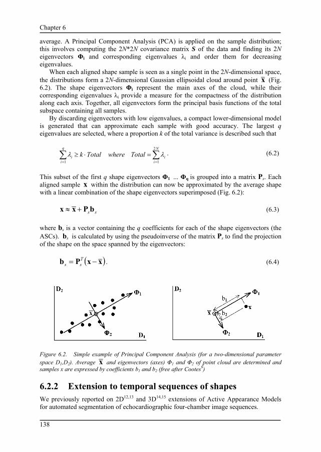
Chapter 6

138

average. A Principal Component Analysis (PCA) is applied on the sample distribution; this involves computing the 2N*2N covariance matrix S of the data and finding its 2N eigenvectors Φi and corresponding eigenvalues λi and order them for decreasing eigenvalues.

When each aligned shape sample is seen as a single point in the 2N-dimensional space, the distributions form a 2N-dimensional Gaussian ellipsoidal cloud around point x (Fig. 6.2). The shape eigenvectors Φi represent the main axes of the cloud, while their corresponding eigenvalues λi provide a measure for the compactness of the distribution along each axis. Together, all eigenvectors form the principal basis functions of the total subspace containing all samples.

By discarding eigenvectors with low eigenvalues, a compact lower-dimensional model is generated that can approximate each sample with good accuracy. The largest q eigenvalues are selected, where a proportion k of the total variance is described such that

∑∑==

=⋅≥N

ii

q

ii TotalwhereTotalk

2

11λλ . (6.2)

This subset of the first q shape eigenvectors Φ1 ... Φq is grouped into a matrix Ps. Each aligned sample x within the distribution can now be approximated by the average shape with a linear combination of the shape eigenvectors superimposed (Fig. 6.2):

ssbPxx +≈ (6.3) where bs is a vector containing the q coefficients for each of the shape eigenvectors (the ASCs). bs is calculated by using the pseudoinverse of the matrix Ps to find the projection of the shape on the space spanned by the eigenvectors:

( )xxPb −= T

ss . (6.4)

Figure 6.2. Simple example of Principal Component Analysis (for a two-dimensional parameter space D1,D2). Average x and eigenvectors (axes) Φ1 and Φ2 of point cloud are determined and samples x are expressed by coefficients b1 and b2 (free after Cootes9)

6.2.2 Extension to temporal sequences of shapes We previously reported on 2D12,13 and 3D14,15 extensions of Active Appearance Models for automated segmentation of echocardiographic four-chamber image sequences.

Chapter 6

139

In the 2D AAM for time sequences (named Active Appearance Motion Model or AAMM), the appearance of the heart is modeled for the entire cardiac cycle by considering the time sequence as a stack of 2D images (time slices). All single-beat sequences are phase-normalized into a fixed number of frames F (16) so that end-diastolic (ED) and end-systolic (ES) frames map to the same frame number (1, 9, and 16 respectively). The other frames are found by nearest neighbor interpolation. In the training set, corresponding shape points on the LV endocardial contour are defined for each time slice based on expert drawn contours. The sequence of contours is considered as a single shape sample (see Fig. 6.3): the shape vectors for all time frames are concatenated in the order of their phase number and further treated just as a single 2D shape vector (2NF-dimensional). Only the 2D coordinates of the points are considered, so, unlike Fig. 6.3 suggests, the third dimension is only implicitly involved.

Principal Component Analysis on the set of training time-sequences renders the mean and eigenvariations of shape of the complete cardiac cycle. In fact it results in an “average heartbeat” and its characteristic motion variations over the complete cycle, as associated to normal/abnormal cardiac contraction. An example is given in Fig. 6.3, where it is shown that a dilation of the apex is typically associated with a reduced displacement at end-systole (hypokinesis).

Figure 6.3. Second eigenvariation of endocardial shape/motion from an AAMM for four-chamber sequences (mean shape (b) plus and minus ((a) and (c)) 3 standard deviations). The objects show contour sequences expressed as a single shape sample. The open ends of the “tube” represent the end-diastolic phases, whereas the constriction in the middle corresponds to end-systole. This eigenvariation is related to typical pathology: apex dilation (panel (a)) is generally associated with reduced apical contraction.

6.3 Experiments 6.3.1 Clinical data Low-dose dobutamine stress echoes were acquired from 129 unselected infarct patients participating in a clinical trial19. For all patients, visual wall motion scoring was performed following the scoring system described in section 6.1 (13 segments, scores from 0 to 3 per segment). Scores per segment and summations (total, per view and per combination of corresponding mid and basal segments) were determined. Several other

Chapter 6

140

clinical parameters associated with wall motion abnormality and severity of myocardial infarction were available:

1. The peak levels of Creatine Kinase (peakCK) and Creatine Kinase - Myocardial Band (peakMB), blood enzyme measures determined from a series of blood samples. PeakCK is a biochemical measure for infarct size, but it may be disturbed by general (non-myocardial) muscle cell damage. PeakMB is a similar measure which is more specific for myocardial damage.

2. The number of pathological Q-waves seen in the ECG within a certain time period (pathQ). This is an indicator for so-called Q-wave infarctions, generally associated with larger infarcted area and more severe LV dysfunction than non-Q-wave infarctions.

3. Standard global LV volume measures: biplane ED and ES volumes and ejection fraction (EDV, ESV, EF), calculated using biplane Simpson’s rule from the manually defined ED/ES contours as specified in section 6.3.2.

4. Sphericity Index for ED and ES, a simple shape measure specifying the ratio of the biplane volume to that of a sphere with the same diameter as the LV’s long axis. A dilated ventricle has an increased Sphericity Index.

6.3.2 Image data and manual border definition From all patients of the set, the transthoracic apical four-chamber and two-chamber image sequences from the baseline stage (non-stress) were available for border detection. Images were digitized from videotape at a resolution of 768*576 pixels with different calibration factors (0.28 to 0.47 mm/pixel). End-diastolic and end-systolic frames were marked by the expert observer. All single-beat sequences were phase-normalized to 16 frames as described in section 6.2.2.

The expert observer manually outlined the contours of the endocardium in ED and ES images of all image sequences. The volumetric measures listed in section 6.3.1 were calculated from these borders. For the remaining images, a semiautomated detection was used based on these ED/ES borders (ECHO-CMS system8). In all cases, the expert applied manual corrections and redetection until completely satisfied with all resulting borders. In total, less than 20% of the contours was manually defined or corrected. Although this contour set can not be considered to be a manually defined set, it is completely expert-validated and therefore a valid independent standard. In total, 4128 ultrasound frames were available with an accompanying expert-validated contour.

6.3.3 Model training and shape analysis The total data set was split randomly into a training set of 65 patients (TRN) and a testing set of 64 patients (TST). Each contour was modeled by 37 landmark points, of which the apex and mitral valve attachments were true anatomic landmarks; the other points were defined by regular subdivision of the manually defined contours. A full-cycle shape representation of all 16 phases thus contained 592 points.

Active Appearance Motion Models for two-chamber and four-chamber were generated from the training set and the ASCs for all training patients were extracted. During shape training, 99.9% of shape variability was kept (Eq. 6.2) to make sure that even the very subtle modes of variation were retained. This resulted in 62 eigenvectors for the two-chamber model and 63 for the four-chamber model and equivalent numbers of ASCs. Also, the four parameters representing the pose of each shape before alignment and its

Chapter 6

141

calibration factor were exported, since it was assumed that at least total size of the shape might be related to pathology. An absolute shape size estimate was calculated from the calibration and two pose parameters and was included in the analysis as well, resulting in 63 and 64 parameters, respectively. Contour sequences of the test patients (TST) were optimally approximated by the AAMM’s shape model by projecting the shapes onto the model (Eq. 6.4) and the corresponding ASCs and pose were extracted. Note that we did not employ AAMM automated border detection, but only its shape modeling. All analyzed contours were from the set described in section 6.3.2.

6.4 Results We used SPSS for Windows version 9.0 (SPSS Inc., Chicago, IL) for statistical analyses on ASCs, VWMS results, and clinical and volumetric parameters. We employed multivariate linear regression and linear discriminant analysis on different combinations of parameters.

6.4.1 Multivariate linear regression with ASCs as independents

Multivariate linear regression was performed for the different sets of ASCs (as independents) against all VWMS results and clinical parameters (as dependents) (Table 6.1). R-square values (the square of the correlation coefficient R) were determined, representing the percentage of the variability in the dependent variable that can be explained by the independent variable(s), the ASCs.

ASCs from the AAMM model appropriate for the dependent variable’s view were employed. So, for VWMS of single or combined two-chamber segments, all 62 ASCs plus the size estimate from the 2-chamber model; for four-chamber segments, all 63 ASCs plus the size estimate from the four-chamber model. For the combined-view results (the apex, the total of all 9 segments from four- and two-chamber, the total of all 13 segments, and all clinical/volumetric parameters), entering all 127 variables resulted in undesired statistical effects like ‘over-training’ (see below). Therefore it was decided to use only the lower 25 ASCs of both views, giving a total of 52 variables. These 25 lower eigenvalues were responsible for about 95% of total shape variabilities (see Eq. 6.2). In the result table, the number of ASCs actually employed in the regression is given.

The regressions were performed both for the collection of all relevant ASCs (giving the best possible prediction, column 4) and for an optimized subset of ASCs (column 5). Here, all ASCs with a low correlation to VWMS were eliminated to get an optimal prediction of VWMS from a minimal number of ASCs (using the ‘backward’ method of independent variable selection in linear regression in SPSS). The resulting R-square value and the remaining number of ASCs are reported. The blood enzyme measures PeakCK and PeakMB are poorly predictable from shape parameters, which is a bit surprising since they are supposed to correlate with infarct size; the ECG parameter PathQ correlates reasonably with ASCs. This is expected, since PathQ is partly associated with infarct severity.

Chapter 6

142

Table 6.1. Multivariate linear regression:

prediction of all clinical and VWMS values by ASCs (independents).

Dependent variable Category View R-square (with all ASCs)

R-sq backward (with #ASCs)

PeakMB All 0.582 (52) 0.356 (8) PeakCK All 0.536 (52) 0.283 (7) PathQ

Clinical

All 0.737 (52) 0.668 (20) Biplane ED Vol. 4C+2C 0.956 (52) 0.949 (19) Biplane ES Vol. 4C+2C 0.944 (52) 0.936 (16) Biplane EF 4C+2C 0.960 (52) 0.952 (28) ED Sphericity 4C+2C 0.915 (52) 0.893 (19) ES Sphericity

Volumes

4C+2C 0.945 (52) 0.930 (17) Total (all 13 segments) All 0.867 (52) 0.838 (24) Total 4C+2C (9 segments) 4C+2C 0.844 (52) 0.781 (15) Total 4C (5 segments) 4C 0.846 (64) 0.786 (19) Total 2C (5 segments) 2C 0.852 (63) 0.798 (21) Septal (2 segments) 4C 0.648 (64) 0.511 (14) Lateral (2 segments) 4C 0.765 (64) 0.668 (22) Anterior (2 segments) 2C 0.757 (63) 0.660 (18) Inferior (2 segments)

VWMS Multiple segments

2C 0.806 (63) 0.701 (15) Apex 4C+2C 0.826 (52) 0.753 (13) Septal basal 4C 0.594 (64) 0.409 (9) Septal mid 4C 0.762 (64) 0.668 (15) Lateral basal 4C 0.627 (64) 0.466 (13) Lateral mid 4C 0.767 (64) 0.675 (24) Anterior basal 2C 0.551 (63) 0.376 (16) Anterior mid 2C 0.757 (63) 0.643 (15) Inferior basal 2C 0.828 (63) 0.744 (20) Inferior mid

VWMS Single segments

2C 0.733 (63) 0.614 (16) Single segment averages ± standard deviation 0.716 ± 0.101 0.595 ± 0.142

(15.7 ± 4.3)

Volume measures (EDV, ESV, EF, ED and ES Sphericity) are very well predicted by

shape (ASCs), which is not surprising at all since these measures are calculated directly from the ED and ES contours, which form a subset of the contours defining the ASCs.

A clear relation was found between ASCs and the different VWMS measures, although sometimes a large number of ASCs (9-24) was needed to get an optimal regression. In the prediction for single segments, most of the basal segments (anterior basal, septal basal and lateral basal) performed relatively bad. The apex performed relatively well, maybe because the combined 4C and 2C parameters were utilized together. From the 2-segment combinations, inferior performed relatively well, probably due to the good performance of the inferior basal segment. These differences between segments may be caused by several factors, either general or specific for this patient set: the distributions of WMA over the segments, the visibility of different segments, or particularities in the VWMS scoring or border tracing. In general, results were relatively better when more segments were combined, which is partly an effect of averaging, partly of the longer total range of results (see Fig. 6.4). Regression plots for the prediction of the total VWMS and for a single segment (Apex) are given in Fig. 6.4.

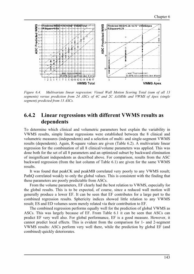
Chapter 6

143

Figure 6.4. Multivariate linear regression: Visual Wall Motion Scoring Total (sum of all 13 segments) versus prediction from 24 ASCs of 4C and 2C AAMMs and VWMS of Apex (single segment) predicted from 13 ASCs.

6.4.2 Linear regressions with different VWMS results as dependents

To determine which clinical and volumetric parameters best explain the variability in VWMS results, simple linear regressions were established between the 8 clinical and volumetric measures (independents) and a selection of multi- and single-segment VWMS results (dependents). Again, R-square values are given (Table 6.2). A multivariate linear regression for the combination of all 8 clinical/volume parameters was applied. This was done both for the set of all 8 parameters and an optimized subset by backward elimination of insignificant independents as described above. For comparison, results from the ASC backward regression (from the last column of Table 6.1) are given for the same VWMS results.

It was found that peakCK and peakMB correlated very poorly to any VWMS result; PathQ correlated weakly to only the global values. This is consistent with the finding that these parameters are poorly predictable from ASCs.

From the volume parameters, EF clearly had the best relation to VWMS, especially for the global results. This is to be expected, of course, since a reduced wall motion will generally produce a lower EF. It can be seen that EF contributes for a large part to the combined regression results. Sphericity indices showed little relation to any VWMS result; ES and ED volumes seem merely related via their contribution to EF.

The combined regression performs equally well for the prediction of global VWMS as ASCs. This was largely because of EF. From Table 6.1 it can be seen that ASCs can predict EF very well also. For global performance, EF is a good measure. However, it cannot predict local effects. This is evident from the comparison for 1- and 2-segment VWMS results: ASCs perform very well there, while the prediction by global EF (and combined) quickly deteriorates.

Chapter 6

144

Table 6.2. Linear regression results of global and segmental VWMS results.

Several clinical measures as independents.

Regression of different VWMS (R-square)

Total Total 4C+2C

Total 4C Lateral Inferior Septal basal

Anterior mid

View: all 4C+2C 4C 4C 2C 4C 2C #segments: Independent:

13 9 5 2 2 1 1

PeakMB 0.133 0.092 0.084 0.063 0.000 0.002 0.047 PeakCK 0.170 0.111 0.106 0.048 0.001 0.004 0.032 PathQ 0.251 0.231 0.256 0.010 0.008 0.004 0.132 EDV 0.224 0.195 0.161 0.119 0.023 0.000 0.019 ESV 0.473 0.446 0.337 0.185 0.045 0.009 0.085 EF 0.786 0.760 0.587 0.214 0.036 0.069 0.156 ED-sphericity 0.052 0.057 0.025 0.037 0.014 0.004 0.002 ES-sphericity 0.149 0.153 0.052 0.120 0.088 0.051 0.001 All 8 combined 0.840

(8) 0.786 (8)

0.656 (8)

0.293 (8)

0.252 (8)

0.181 (8)

0.266 (8)

All 8 backward (with #pars)

0.835 (4)

0.777 (2)

0.649 (6)

0.281 (4)

0.243 (5)

0.141 (4)

0.235 (3)

ASCs backward (with #pars)

0.838 (24)

0.781 (15)

0.786 (19)

0.668 (22)

0.701 (15)

0.409 (9)

0.643 (15)

6.4.3 Linear discriminant analysis Discriminant analysis was performed to find optimal classification of WMA from a minimal number of ASCs. Since VWMS is a visually established, subjective assessment with considerable observer variability, wall motion score values were grouped into only two classes for these classification experiments. For single segments and combinations of 2 segments, a distinction was made between normal and abnormal wall motion, where a score of 0 was considered normal, and all scores >0 abnormal. For combinations of 5 and more segments, where many scores are summed, such a distinction would result in very biased or even empty classes (note that the patient set contained only infarct patients and no normals). Therefore, for these multi-segment combinations a distinction into mild and severe WMA was made. For groups of 5 segments, a summed score >1 was considered severe; for the 9-segment combination of 4C and 2C segments, >3; and for the total score of 13 segments, >5. This resulted in reasonably balanced groups in most cases.

Classification was performed in three different experiments, representing an ‘ideal’ situation, a ‘worst-case’ situation and a mixed case. As described above, the patient set was split in a TRN set (n=65) and a TST set (n=64). The shape model was trained from the TRN set only and thus is capable of modeling the TRN shapes exactly; so the ASCs describe these shapes perfectly. For the TST set, the shapes were projected on the shape model and approximated. However, these ASCs may not perfectly describe the shapes, since the training was performed on a limited set only and may not completely cover all variability in the TST set. The ASCs derived for the TST set may also have slightly different characteristics with respect to WMA than those from the TRN set.

To assess the differences between such situations, three experiments were performed. First of all, the classification was performed on the TRN set (column 5 in Table 6.3), representing ASCs from a ‘perfect’ shape model (corresponding to a shape model trained from a very large and well-balanced patient set). The classifier was trained using a leave-

Chapter 6

145

one-out approach: in turn, each of the training cases was left out, the optimal discriminant function was determined from the other cases, and tested on the one remaining case. This was repeated n-1 times. This approach guarantees independence between training and test cases. Leave-one-out experiments are listed by L-1-O in Table 6.3.

Secondly, a classifier was trained on ASCs from all TRN cases and tested on those of all TST cases (column 6 in Table 6.3). This is a worst-case real-world experiment: both shape model and classifier are trained from a limited training set and tested on completely ‘new’ shapes.

Thirdly, an intermediate real-world situation is simulated using the whole patient set (TRN+TST, n=129): the shape model is trained on TRN only, but the classifier is trained on ASCs from both the TRN set (perfect) and TST set (imperfect), again using a leave-one-out approach (column 4 in Table 6.3). This classifier will be tuned better to the different ASC characteristics of the TST set. The classifier may also perform better because of the larger set. A discriminant function is determined based on a linear combination of the predictor variables that provides the best discrimination between the groups. The independent predictor variables were entered into the analysis in a stepwise fashion. In each step, the variable is entered that minimizes the sum of the unexplained variation between groups. Variables may be entered or removed if the significance level of their F value passes a given entry/removal threshold. The process continues until no more variables can be entered or removed. No prior probabilities were computed from the training group sizes, so all a priori group probabilities were equal.

Linear discriminant analysis results on the prediction of VWMS are listed in Table 6.3. For comparison, the ASC predictions were set against the best predictor from the clinical parameters as listed in Table 6.2: Biplane EF. Note that this parameter should not be considered a gold standard for segmental VWMS prediction since it is associated only with global LV function. Three different experiments were performed as described above (columns 7, 8, 9).

Table 6.3 shows good ASC classification of WMA (78%-95% correctness for TRN+TST set) for both single (on average, 85%) and combined (multiple) segments. The numbers of ASCs employed were generally low (on average, 10 or 8 for single segments) except for a few combined cases where the discriminant seemed to ‘over-train’ itself in order to cover 100% of the variation in the training data. In such cases, it would be possible to limit the number of included ASCs (probably at the cost of a lower performance). In the hardest test (column TST, shape model and classifier training on the TRN set and test on the TST set), still a 74% correctness for single segments was achieved, which certainly is a promising result considering the variabilities in VWMS. The TRN test suggests that with an optimal shape model, a segmental correctness of up to 89% is feasible.

ASCs predict WMA better than EF in most cases, both for combined segments and single segments. As expected, the difference is largest for single segments, where EF predicts not much better than a random choice (50%). In fact it could be seen as a biased guess: a reduced EF can tell that there must be a wall motion abnormality somewhere for a specific case, but it obviously cannot tell you where. For the Total TRN+TST set and the TRN set, ASC performs better in all cases; for the TST set, EF is sometimes slightly better, but this may well be an accidental effect. For all three sets, the ASC single-segment average was significantly higher than the corresponding EF average, according to a single-sided paired t-test at the 1% level.

Chapter 6

146

Table 6.3. Classification correctness of wall motion abnormality

for different segments and combinations. Classification correctness (%) Predicted from AAM Shape

Coefficients (#ASCs employed)

Predicted from Biplane EF

VWMS (criterion)

Category Views (# segments)

TRN+TST (L-1-O)

TRN (L-1-O)

TST TRN+ TST (L-1-O)

TRN (L-1-O)

TST

Total (>5) All (13) 90% (20) 100% (35) 77% (35) 79% 85% 73% Total 4+2 (>3)

4C/2C (9) 89% (14) 89% (11) 70% (11) 79% 75% 83%

Total 4c (>1) 4C (5) 85% (15) 88% (13) 78% (13) 74% 79% 77% Total 2c (>1) 2C (5) 94% (9) 100% (21) 97% (21) 61% 65% 64% Septal (>0) 4C (2) 78% (12) 100% (28) 67% (28) 67% 66% 72% Lateral (>0) 4C (2) 78% (9) 82% (10) 70% (10) 71% 69% 73% Anterior (>0) 2C (2) 86% (14) 94% (11) 73% (11) 67% 68% 69% Inferior (>0)

VWMS Multiple segments

2C (2) 85% (16) 94% (16) 75% (16) 49% 54% 45% Apex 4C/2C 95% (17) 94% (7) 81% (7) 74% 75% 72% Septal basal 4C 78% (7) 87% (10) 70% (10) 64% 74% 58% Septal mid 4C 86% (10) 92% (12) 73% (12) 67% 63% 70% Lateral basal 4C 85% (6) 86% (8) 64% (8) 67% 71% 63% Lateral mid 4C 78% (10) 77% (6) 70% (6) 73% 69% 75% Anterior basal

2C 88% (2) 95% (3) 95% (3) 75% 86% 86%

Anterior mid 2C 88% (14) 94% (11) 75% (11) 69% 68% 70% Inferior basal 2C 84% (12) 85% (5) 72% (5) 57% 55% 58% Inferior mid

VWMS Single segments (criterion: >0)

2C 81% (14) 91% (12) 66% (12) 55% 63% 50% Single segment averages ± standard deviation

84.7±5.6% (10.2±4.7)

88.9±5.9% (8.2±3.2)

74.0±9.4% (8.2±3.2)

66.6 ± 7.1%

69.4 ± 8.8%

66.7 ± 10.8%

Two-chamber results were generally superior to four-chamber; this may be attributed to the distribution of WMA over the segments, where the two-chamber segments saw a wider range of VWMS scores.

Note that the prediction of total VWMS for all 13 segments is at least as good as that of the 9 segments (four- and two-chamber only). This may sound strange, since the extra segments (belonging to the long axis view) are not included in the ASCs at all. However, this may be attributed to the high correlation between the long-axis segments and their neighbors in the four and two chamber views, which are supplied by the same coronary arteries.

6.5 Discussion As the most important result from this study, we can conclude that ASCs are indeed suitable for classification of wall motion abnormalities. It also shows that endocardial contours (by themselves) may be sufficient to allow automated classification/prediction of VWMS, and that our proposed approach of endocardial border detection and subsequent shape analysis is feasible in principle.

Another interesting result is that an ASC shape analysis can assess the quality of sets of contours through direct correlation with clinical parameters. The percentage of variability of the clinical parameter explained by a linear combination of ASCs (R-square)

Chapter 6

147

is a useful measure for this. This also allows comparisons between different sets of contours (e.g. manual vs. automatically detected). Apart from these interesting first results, several issues remain to be treated.

6.5.1 Manually versus automatically detected contours Of course, it remains to be shown that the described approach will also work on automatically determined contours (preferably determined by an AAM). All above experiments were performed on an ‘expert-verified’ contour set (section 6.3.2.). This set was in fact for >80% derived semiautomatically, but the most important contours (ED and ES) were defined manually by the expert and subsequently detected contours were corrected, so that we consider it closer to a manually defined set. We only performed some preliminary experiments on contours that were detected fully automatically by AAMM, but results were clearly less good than for the original set. This may be attributed to several factors, but most likely small errors in the detection tend to obscure the typical patterns seen in the manual contours. As we have seen with earlier studies13,15,17, it seems that AAMs tend to stay a bit too close to the average shape/motion patterns. They generate quite a good overall approximation of the shapes (in terms of distances and area differences), but fail to follow the finer details. Luckily, there are still many possibilities to optimize the border detection, e.g. by a hybrid combination with Active Shape Models and/or Dynamic Programming, as described earlier17. This is a subject of further studies. An alternative may be to adjust for the change in patterns by training another shape model from the automatically detected shapes and correlate its ASCs directly to the visual wall motion scores.

6.5.2 Limitations of VWMS It should be stressed that the strength of the found relations must be seen in the light of the large inherent uncertainties and variabilities associated with VWMS itself. The fact that on average 60% of the total variability in single-segment VWMS can be explained from a limited number (~16) of ASCs is actually a strong result.

VWMS is in fact a qualitative measure made semiquantitative, which makes it less suitable for a linear regression approach as applied here. Single segments can only have a few different scores and due to the small numbers of examples the distributions are quite irregular, so correlations and linear regression may be weak. Furthermore, Visual Wall Motion Scoring is known to be subjective and operator-dependent. Even in highly controlled multi-center studies it has been shown that inter-institution variability can be high. Although such numbers cannot be compared directly, e.g. 73% agreement on normality/abnormality of a complete dobutamine stress test was reported2.

One should realize that automating or imitating VWMS is not the main goal. VWMS is in fact a tool to predict the presence of coronary artery disease, and its virtues for that have been assessed well by comparison to established clinical measures, such as quantitative coronary angiography. It has also been compared to competing techniques like the nuclear imaging thallium stress test, ECG stress testing etc. Therefore, it would be most interesting to relate ASC shape analysis directly to quantitative coronary angiography to determine its sensitivity and specificity for detection of coronary artery disease. It could also be related to other established measures of coronary or myocardial pathology.

Chapter 6

148

6.5.3 Relations with clinical parameters The clinical parameters peakCK, peakMB and pathQ were found to be only weakly related to both VWMS results and ASCs. For all three we can state that these are measures of global pathology/infarct size, with many sources of errors, and not necessarily directly coupled to wall motion in the views involved.

From the volumetric parameters it was found that only EF correlated well to global VWMS. Sphericity indices showed poor relations, and biplane volumes offered no additional value. Predictive power for segmental VWMS was very low, as can be expected.

However, these weak relations stress the fact that VWMS and ASCs are indeed closely related, and that both global and segmental VWMS can be predicted from ASCs. The weak relations also rule out the possibility that by using a large number of ASC variables we could predict almost anything - this obviously is not the case. The found relations are real and not statistical artifacts. Furthermore, the fact that ASCs can predict any of the volumetric parameters is another proof that they cover the properties of shape well.

6.5.4 Alternatives for assessment of wall motion abnormalities

In this study, we have chosen to analyze endocardial borders to detect wall motion abnormalities. As mentioned, alternative approaches exist, such as Tissue Doppler Imaging (TDI) or the derived Strain Rate20 and Strain21 Imaging. Without going into details, we can state that these techniques are limited as well. In particular, we have shown that combining longitudinal velocities from TDI with radial velocities from endocardial border detection may increase success6.

Another possibility is the addition of epicardial contours. In visual wall motion scoring, thickening of the myocardium is an important clue for normal contraction. Assessment of myocardial thickness/thickening would involve both endocardium and epicardium. However, the epicardium is often hard to delineate precisely from echocardiographic data. Although an AAM approach allows for multiple contours to be modeled and detected simultaneously, it remains to be studied whether this will improve WMA classification.

6.5.5 PCA limitations, extensions and alternatives The described PCA-based approach has some limitations. As any training-based approach, its reliability depends on the range of variabilities covered in the training set: it should include normals and sufficient cases of expected pathologies. Furthermore, the result is limited by the quality and reproducibility of the training contour data: accurately validated borders on substantially larger data sets are required.

PCA assumes Gaussian distributions. Provided that the example set is representative of the variability in the population and the distribution can be approximated by a high-dimensional Gaussian ellipsoid, an AAM can generate any statistically plausible intermediates10. If the distribution is disjunct or very skewed, the model may generate implausible intermediates or may fail to cover the full range of variability.

In this study, almost all shape variation (99.9%) from the training set was included in the models and analyses, except for the combined views where 95% was used. Removing

Chapter 6

149

a larger percentage of variation would result in a more generalized and compact model. However, we should probably use larger training sets to achieve good generalization.

In this study, separate shape models for four-chamber and two-chamber images were trained. In fact, AAMs can use coupled models which incorporate the different views of the same object into a single model22. This will automatically include interrelated shape properties in the eigenvariations.

PCA will provide an optimal description of variability over a set, but is not aimed at an optimal classification or localization. This is a reason why relatively many ASCs are involved in single- and multi-segment VWMS prediction or WMA classification. For this purpose, Independent Component Analysis (ICA) may form a good alternative for PCA, allowing to decompose shapes into components that describe very local shape behavior. This is a subject of further study.

PCA shape modeling is an inherent part of AAM methods, and it is therefore attractive to combine AAM border detection with ASC shape analysis. However, the ASC analysis can be applied completely independent of AAMs and can be combined with any type of border detection.

6.5.6 Limitations of the study setup The setup of this study was limited in several aspects. Only infarct patients were included, while for a good unbiased general shape model training and ASC discriminant function determination, other pathologies and normals should be included as well. From the stress echoes, only resting two- and four-chamber images were used. Adding long-axis and short-axis images may improve results. The same approach should be tested on the dobutamine images, and on the assessment of rest/stress differences. A combined shape model for rest and stress images could be trained as well.

For the statistical analyses, only linear regression and linear discriminant classifiers were employed, while VWMS is a very nonlinear measure. Other nonlinear classifiers may achieve better results.

6.6 Conclusions AAM shape coefficients can describe regional wall motion abnormality and can be used for automated classification of such abnormalities with good accuracy: for single segments, on average 89% correctness was achieved against an expert observer in case of a ‘perfect’ shape model. With a suboptimal shape model, 85% correctness was obtained. Considering the inaccuracy and high inter- and intra-observer variability of visual scoring, the achieved results suggest that automated wall motion scoring is feasible.

VWMS and endocardial border shape/motion patterns are shown to be closely related; if accurate automated border detection is available, this opens the way to fully automated classification of wall motion abnormality in echocardiograms.

ASC shape analysis is also a powerful tool for evaluating the relation of shapes with arbitrary clinical parameters or for comparing the quality of different contour sets by direct comparison to clinical measures.

Chapter 6

150

Acknowledgments This research was supported in part by the Ministry of Economic Affairs, the Netherlands, under grant number BTS00123. Data analysis support provided by Gerard van Burken is gratefully acknowledged.

References 1. Th. H. Marwick, Stress echocardiography, Kluwer, Dordrecht, 1994. 2. R. Hoffman, H. Lethen, Th. H. Marwick et al., "Analysis of interinstitutional observer agreement in

interpretation of dobutamine stress echocardiograms", J. Am. Coll. Cardiol. 27, pp. 330-336, 1996. 3 . P. A. Assman, C. J. Slager et al., "Comparison of models for quantitative left ventricular wall motion

analysis from two-dimensional echocardiograms during acute myocardial infarction", Am. J. Cardiol. 71, pp. 1262-1269, 1993.

4. S. J. Fry, P. Hunziker, H. Bosch et al., "Automated echocardiographic confirmation of regional wall motion ab-normalities: quantitation of continuous LV volume", abstract, J. Am. Coll. Cardiol. 31 (suppl. A) p. 56A, 1998.

5 P. Hunziker, D. Yuan, L. Schöb et al., "Objective and quantitative stress echo analysis to diagnose coronary disease using model-based image processing", abstract, J. Am. Coll. Cardiol. 35 (Suppl A) p. 431A, 2000.

6. P. Cain, L. Short, T. Baglin et al, "Development of a fully quantitative approach to the interpretation of stress echo-cardiography using radial and longitudinal myocardial velocities", J. Am. Soc. Echocardiogr. 15, pp.759-767, 2002.

7. J. G. Bosch, L. H. Savalle et al., "Evaluation of a semiautomatic contour detection approach in sequences of short-axis two-dimensional echocardiographic images", J. Am. Soc. Echocardiogr. 8, pp. 810-821, 1995.

8. J. G. Bosch, G. van Burken et al, "Overview of automated quantitation techniques in 2D echocardiography", in What's new in cardiovascular imaging, J. Reiber and E. v.d. Wall, eds., pp. 363-376, Kluwer, Dordrecht, 1998.

9. T. F. Cootes, G. J. Edwards and C. J. Taylor, "Active Appearance Models.", in European Conf. Computer Vision, H. Burkhardt and B. Neumann, eds., pp. 484-498, Springer, Berlin, 1998.

10. T. F. Cootes, C. J. Taylor, "Statistical models of appearance for medical image analysis and computer vision", in Medical Imaging 2001: Image Processing, M. Sonka, K. M. Hanson, eds., Proc. SPIE 4322, pp. 236-248, 2001.

11. T. F. Cootes, A. Hill, C. J. Taylor and J. Haslam, "Use of active shape models for locating structures in medical images", Image and Vision Computing 12, pp. 355-366, 1994.

12. H. G. Bosch, S. C. Mitchell, B. P. F. Lelieveldt et al., "Active Appearance Motion Models for endocardial contour detection in time sequences of echocardiograms", in Medical Imaging 2001: Image Processing, M. Sonka, K. M. Hanson, eds., Proc. SPIE 4322, pp. 257-268, 2001.

13. J. G. Bosch, S. C. Mitchell, B. P. F. Lelieveldt et al., "Automatic segmentation of echocardiographic sequences by Active Appearance Motion Models" IEEE Trans. Med. Imaging 21, pp. 1374-1383, 2002.

14. J. G. Bosch, S. C. Mitchell, B. P. F. Lelieveldt, et al., "Fully automated endocardial contour detection in time sequences of echocardiograms by three-dimensional Active Appearance Models", in Medical Imaging 2002: Image Processing, M. Sonka, J. M. Fitzpatrick, eds., Proc. SPIE 4684, pp. 452-462, 2002.

15. S. C. Mitchell, J. G. Bosch, B. P. F. Lelieveldt, et al., "3-D Active Appearance Models: segmentation of cardiac MR and ultrasound images", IEEE Trans. Med. Imaging 21, pp. 1167-1178, 2002.

16. A. D. Parker, A. Hill, C. J. Taylor et al., "Application of point distribution models to the automated analysis of echocardiograms", in Computers in Cardiol., A. Murray, ed., pp. 25-28, IEEE, Los Alamitos, CA, 1994.

17. S. C. Mitchell, B. P. F. Lelieveldt et al., "Multistage hybrid Active Appearance Model matching: segmentation of left and right ventricles in cardiac MR images", IEEE Trans. Med. Imaging 20, pp. 415-423, 2001.

18. C. Goodall, "Procrustes methods in the statistical analysis of shape," J. Royal Stat. Soc. B., 53, pp. 285-339, 1991.

19. F. Nijland, O. Kamp, P. M. J. Verhorst, W. G. de Voogt, H. G. Bosch, C. A. Visser, "Myocardial viability: impact on left ventricular dilatation after acute myocardial infarction", Heart 87, pp. 17-22, 2002.

Chapter 6

151

20. A. Heimdal, A. Stoylen, H. Torp, T. Skjaerpe, "Real-time strain rate imaging of the left ventricle by ultrasound", J. Am. Soc. Echocardiogr. 11, pp. 1013-1019, 1998.

21. G. Armstrong, A. Pasquet, K. Fukamachi, et al., "Use of peak systolic strain as an index of regional left ventricular function: Comparison with tissue Doppler velocity during dobutamine stress and myocardial ischemia", J. Am. Soc. Echocardiogr. 13, pp. 731-737, 2000.

22. C. R. Oost, B. P. F. Lelieveldt, G. Koning, M. Sonka, J. H. C. Reiber, “Left ventricle contour detection in X-ray angiograms using Multi-View Active Appearance Models”, in Medical Imaging 2003: Image Processing, M. Sonka, J. M. Fitzpatrick, eds., Proc. SPIE 5032, pp. 394-404, 2003.

Chapter 6

152

153

Chapter 7

Clinical and research applications

of developments in automated echocardiographic contour detection.

Johan G. Bosch

Division of Image Processing, Department of Radiology, Leiden University Medical Center, Leiden, The Netherlands.

Chapter 7

154

Chapter 7

155

7.1 Introduction This thesis describes the results of our echocardiographic image analysis research carried out over many years (1987-2004). Over this extended period, the main line of research was the detection and tracking of the endocardial border in echocardiographic images and sequences, but the intended applications and the approaches evolved considerably with time. Meanwhile, other researchers applied our developments in clinical studies. Furthermore, we investigated new application opportunities that often resulted in separate branches of research. Therefore, this chapter presents an overview of our work within its historical context, sketches the connections between the previous chapters and provides a broader view.

In Fig. 7.1, a timeline is presented marking some important general developments in echocardiography and image processing, together with the primary and secondary research projects discussed in this chapter.

Figure 7.1. Timeline of developments: echocardiography, echocardiographic image processing, and primary and secondary developments at LKEB.

Chapter 7

156

First, an overview of the primary developments over the years is given in section 7.2, with a summary of clinical results and applications†. The next part of this chapter (section 7.3) reports on several sidesteps that have spawned significant results. These are discussed topically in more or less chronological order. Finally, in 7.4 we will present conclusions and some visions of the future.

7.2 Overview of the main line of research and its applications

Over the years, several projects were performed that constituted the central line of research. The subjects evolved from straightforward contour detection in single images to more complex and advanced image analysis approaches. This corresponds to the general evolution of image processing from the classical data-driven (bottom-up) approaches, via model driven (top-down) approaches to modern analysis-by-synthesis and knowledge-based methods.

7.2.1 Short-axis single-frame endocardial contour detection

Our earliest work in echocardiographic analysis focused on endocardial detection in single-frame short-axis images from transesophageal echocardiography (TEE). Two-dimensional transesophageal echocardiography was still a relatively new technique, developed to a large extent by Nicolaas Bom PhD and Charles T. Lancée PhD1 at the Department of Experimental Echocardiography of the Thoraxcenter, Erasmus University Rotterdam. Image quality of TEE echo was at that time significantly better than that of transthoracic echo (TTE), due to the lack of obstructions like ribs and lungs, the proximity to the heart (allowing the use of higher ultrasound frequencies) and the absence of subcutaneous fatty tissue in the ultrasound pathway.

The first publications on automated border detection in echocardiograms started to appear in the early 1980’s (e.g.2-4, see ch. 1 for overviews) but methods were still very primitive. Preliminary experiments on automated border detection in TEE images were performed at the Thoraxcenter by Lancée et al.5, based on the work of Grube et al.6. At the same time and place, the Laboratory for Clinical and Experimental Image Processing (LKEB), led by Johan H.C. Reiber, PhD, performed research on automated image analysis for X-ray angiography. This resulted in automatic methods for LV angiographic lumen detection and coronary artery analysis7 that were implemented in the CAAS system (commercialized by Pie Data Medical, Maastricht, the Netherlands).

Around 1986, Peter J. van Leeuwen at the LKEB demonstrated that the dynamic programming (DP) algorithms that were successful in angiography8 could be adapted for use in ultrasound as well. This initiated the project on which the author started working on the subject of echocardiographic image analysis, funded by the Dutch Heart Foundation † In this chapter, many references to other researchers are made. For most cooperators, the scientific titles (PhD, MSc, MD) are given that were applicable at the time of the cooperation. Some titles were omitted if unknown or uncertain. For clarity, all clinical cooperators are indicated at least by the title “MD”, irrespective of their exact scientific title. We apologize to all whose titles are not stated correctly.

Chapter 7

157

(NHS 86.080, “Automatic analysis of transesophageal echocardiograms” 1987 - 1990). The anticipated automated echocardiographic detection technique was primarily intended to support automatic transesophageal monitoring of cardiac parameters like ejection fraction (EF) and cardiac output (CO), for use in anesthesiology during surgery. This was clinically explored in cooperation with Marc E.R.M. van Daele MD and Jos R.T.C. Roelandt MD PhD at the Thoraxcenter9,10. This intended use also necessitated a real-time implementation. Therefore, we started a separate project on the development of special real-time contour detection hardware, which is further described in section 7.3.2.

The technique that was developed in the NHS project11-15 consisted of a DP approach (see ch. 3.2) based on a circular model of the short-axis endocardial contour. The user would indicate a centerpoint with the mouse, a circular model with fixed radius was applied (Fig. 7.2) and the image was resampled with low resolution in a broad ring-shaped strip around this model. The samples were placed in a scan matrix and costs were assigned per node as a linear combination of grey value averages, distances from the model, a first derivative in normal direction to the model and an absolute first derivative in tangential direction. Using DP, a closed contour was found (chapter 3.2.3.2), which was subsequently used as a model itself for resampling over a narrow strip with higher resolution, to reach a better approximation of the true border. A typical result is shown in Fig. 7.3.A. This technique was a quite advanced model-driven approach in comparison to others reported in that period (see ch. 1), that used purely bottom-up (data driven) approaches, such as thresholding16, morphological operations17 or a radial search for a strong edge, followed by edge linking6. Also, we entrusted our approach to be more successful than methods based on simulated annealing18 or on snakes or active contours19, since it lacked the convergence problems and instabilities associated with those iterative approaches, and directly led to an optimal solution.

In the first evaluations, we showed that the inter- and intra-observer variability in the automatic contours (caused by variations in the indicated centerpoint) was below 1.42 mm for ED and ES images of 10 patients11-14. In a further study9,10 in 10 patients, cross-sectional areas of ED and ES frames taken at 4 intervals were analyzed manually and by our DP technique. Areas correlated well between manual and DP contours (r = 0.97) and to thermodilution results; a slightly lower beat-to-beat variation was found for DP (DP 4.5%, manual 5%, thermodilution 9%) for the good-quality images, but in suboptimal images the detection was sensitive to artifacts.

A more elaborate evaluation15,20 was performed on standard-quality TEE images of 12 patients, each with 4 sequences of 5 consecutive beats (480 ED and ES images). Manual and automatic contours were compared by calculating local distances (in mm) between pairs of corresponding contours using a 100-point modified centerline analysis21. Automatic contours with and without corrections were analyzed. Also, inter- and intra-observer variabilities were calculated for all 3 sets (manual, DP, corrected) on 40 images. Distances between manual and automatic contours were 2.8 ± 2.4 mm, indicating that the automatic contours were slightly but systematically smaller; the manual contours still had lower observer variability (1.1mm vs. 2.1mm). The corrected contours were closer to the manual contours (2.0 ± 1.8mm) and had an observer variability of 1.6mm. These results were encouraging, given the challenges, but it was clear that this single-frame DP approach could not yet replace manual drawing.

Chapter 7

158

Figure 7.2. Single-frame short-axis contour detection procedure (from12). A. Original image with manually placed circular model. B. Path search. Left upper: resampled image from strip around model. Left lower: array of

cost values. Right: minimum cost path. C. Detected contour is applied as a model in the second iteration with resampling over a

narrower range. D. Final contour after second iteration.

We experimentally applied this DP approach to several other types of images as well, including short-axis TTE, open-chest epicardial echoes, IVUS22-25 and short-axis MRI (Fig. 7.3.B-D). Some of these experiments, performed with adapted versions of our algorithmic implementations for echo, formed the onset for the development of similar detection approaches in other domains, like the methods for IVUS developed by W. Li (see 7.3.1). Automated detection for MRI based on DP later was investigated categorically at our laboratory by Rob J. van der Geest et al., which resulted in the successful MASS system for semiautomatic analysis of MRI images26.

7.2.2 Contour detection and tracking in echocardiographic sequences

The DP approach was evaluated with promising results, as described above. However, the complexity and ambiguity of the still-frame images formed a serious problem and left a considerable margin of variability and uncertainty. The general image quality of B-mode echocardiograms was (and actually still is) insufficient to allow reliable segmentation of

Chapter 7

159

Figure 7.3. Applications of single-frame DP algorithm to short-axis TEE and other domains. A. Short-axis TEE (from13). B. Intraoperative epicardial short-axis echo. C. IVUS (from24). D. MRI short-axis. single (still-frame) images. Even human observers have great difficulties to reach a consistent, reliable segmentation on single images; in practice, cardiac images are always reviewed in motion before a single image is manually segmented. It is widely known that an echo image in motion (directly acquired, or played back from videotape or in digital cineloop) is much easier to interpret than a single still image. The coherence between consecutive images, the difference in temporal behavior of tissue and artifacts and the information redundancy facilitate in distinguishing subtle anatomical structure and detail from clutter, artifacts, noise etc. Therefore, the logical next step was the development of methods for time sequences of images. Analyzing a sequence allows the integration of such coherence and application of models of both endocardial shape and motion.

These subjects were investigated in a project funded by the Technology Foundation, the Netherlands (STW, project LGN92.1706, 1990-1995; “Development, implementation and evaluation of an automated analysis station for quantitative echocardiography”). Final development into a commercial system was funded by Medis medical imaging systems bv, Leiden, the Netherlands (1995-1996).

Chapter 7

160

7.2.3 Edge-based endocardial border detection for short axis sequences

First, the detection of short-axis sequences was taken up. This work was closely coupled to our efforts to realize real-time detection, as described in 7.3.2. However, for solving the general case we are not restricted by the severe limitations of the real-time monitoring application (extreme robustness, total automation, high and predictable speed, lack of user guidance or correction).

The detection approach that we have developed for short-axis image sequences and its evaluation is described in detail in chapter 2 of this thesis. It uses closed-contour dynamic programming (see 3.2.3.2) with an edge-based cost function and requires only the indication of a center point of the left ventricle, or the manual drawing of a first contour approximation. A feed-forward geometric model prediction (3.2.3.7) is used: the contour detected in one image is smoothed and used as the model for the next and/or previous image. The width of the search range is matched to the expected maximal frame-to-frame wall displacement. This detection was described in several papers27-32 and evaluated on 20 patients with good results: the automated contour areas were shown to correlate very well with manually defined contours29:

Semiautomatic = 1.01 * Manual + 5.58%; r = 0.989, SEE = 11.9%. Furthermore, inter- and intra-observer variability of the automated method were significantly smaller than those of manual delineation. Manual correction was needed in only 18% of images. Total analysis time was reduced by a factor of 5 in comparison to manual analysis.

7.2.4 Edge-based detection for major axis sequences After the realization of the short-axis detection, we turned our attention to the analysis of the other cross sections of clinical interest. In particular the apical four-chamber and two-chamber cross sections allow a much broader range of parameter calculations than the short-axis cross section, especially for volume and wall motion analyses.

In major-axis cross sections (apical four-chamber, apical two-chamber, parasternal long axis), two specific issues make detection of the endocardium more difficult than for short-axis images:

1. The geometric model is more complex: a hemielliptic, open shape, with complex dynamic behavior (e.g. the moving mitral valve plane).

2. The border appearance (intensity patterns) can be very different per region; and the strongest edge is often not the desired one. Edges are obscured by noise, artifacts, dropouts etc. Often, the cardiologist wants to track a structure that is not associated with an edge at all (e.g. because of trabecular structure, imaging artifacts, or foreshortening).

Initially, the technique described above for short-axis detection was extended directly towards major-axis images, addressing only the first issue. Instead of a single center point, three markers were used: an apical marker and two mitral valve points. A hemi-elliptic model was fit through these three points, and an edge-based dynamic programming detection comparable to the method described for short-axis views was applied. The model propagation was also improved: instead of simply using the previous contour as a model, a weighted average between the default model shape and the previous detected contour could be used33. This prevented uncontrolled propagation of local shape

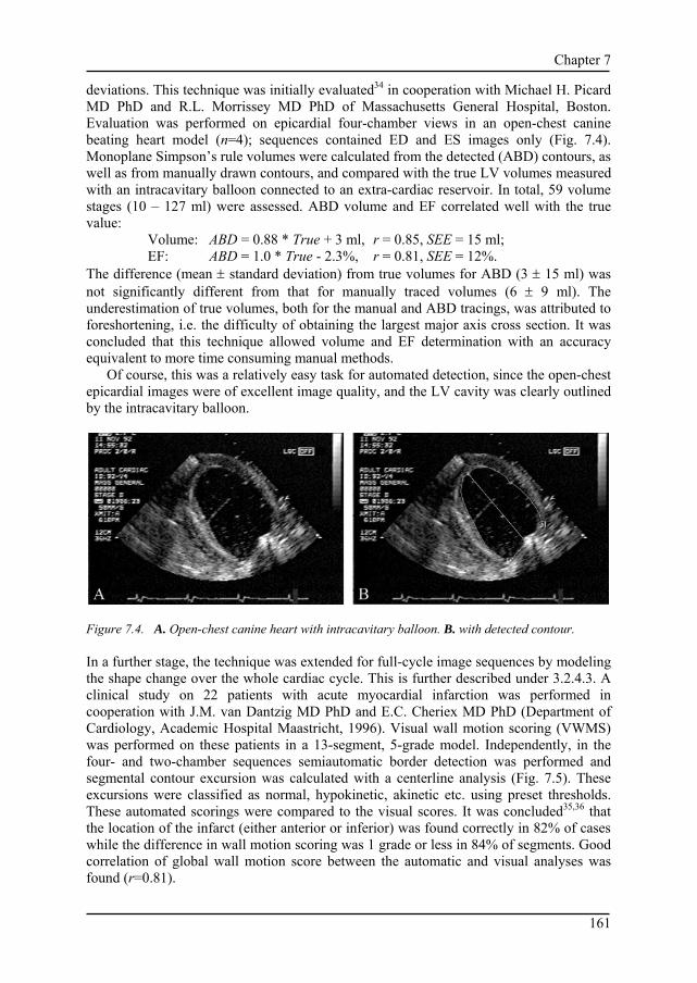
Chapter 7

161

deviations. This technique was initially evaluated34 in cooperation with Michael H. Picard MD PhD and R.L. Morrissey MD PhD of Massachusetts General Hospital, Boston. Evaluation was performed on epicardial four-chamber views in an open-chest canine beating heart model (n=4); sequences contained ED and ES images only (Fig. 7.4). Monoplane Simpson’s rule volumes were calculated from the detected (ABD) contours, as well as from manually drawn contours, and compared with the true LV volumes measured with an intracavitary balloon connected to an extra-cardiac reservoir. In total, 59 volume stages (10 – 127 ml) were assessed. ABD volume and EF correlated well with the true value:

Volume: ABD = 0.88 * True + 3 ml, r = 0.85, SEE = 15 ml; EF: ABD = 1.0 * True - 2.3%, r = 0.81, SEE = 12%.

The difference (mean ± standard deviation) from true volumes for ABD (3 ± 15 ml) was not significantly different from that for manually traced volumes (6 ± 9 ml). The underestimation of true volumes, both for the manual and ABD tracings, was attributed to foreshortening, i.e. the difficulty of obtaining the largest major axis cross section. It was concluded that this technique allowed volume and EF determination with an accuracy equivalent to more time consuming manual methods.

Of course, this was a relatively easy task for automated detection, since the open-chest epicardial images were of excellent image quality, and the LV cavity was clearly outlined by the intracavitary balloon.

Figure 7.4. A. Open-chest canine heart with intracavitary balloon. B. with detected contour. In a further stage, the technique was extended for full-cycle image sequences by modeling the shape change over the whole cardiac cycle. This is further described under 3.2.4.3. A clinical study on 22 patients with acute myocardial infarction was performed in cooperation with J.M. van Dantzig MD PhD and E.C. Cheriex MD PhD (Department of Cardiology, Academic Hospital Maastricht, 1996). Visual wall motion scoring (VWMS) was performed on these patients in a 13-segment, 5-grade model. Independently, in the four- and two-chamber sequences semiautomatic border detection was performed and segmental contour excursion was calculated with a centerline analysis (Fig. 7.5). These excursions were classified as normal, hypokinetic, akinetic etc. using preset thresholds. These automated scorings were compared to the visual scores. It was concluded35,36 that the location of the infarct (either anterior or inferior) was found correctly in 82% of cases while the difference in wall motion scoring was 1 grade or less in 84% of segments. Good correlation of global wall motion score between the automatic and visual analyses was found (r=0.81).

Chapter 7

162

Figure 7.5. (see color suppl.) Typical regional wall motion graphs showing abnormal motion in the basal and mid inferior wall (segments 1-40). Two-chamber view from the Maastricht study. The five segmental wall motion scores were: dyskinetic, akinetic, normal, normal, normal, both for the visual scoring and the score assigned by the automated border detection.

This was the first step towards automatic wall motion scoring and the results were very encouraging, notwithstanding the fact that we used an overly simple approach for translating wall displacement to VWMS: the same absolute displacement threshold for all segments, no corrections for overall motion or heart size, etc. However, the quality of the detection could still be improved; it proved quite hard to reach consistent segmentations with this edge-based detection method. Overall, almost 4 contour corrections were needed per cardiac cycle. In internal evaluations of the performance of the detection, it was found that the contour detection worked well as long as the endocardial border was clearly visible. The main limitations were found in areas of considerable dropout (often the lateral wall) where significant temporal inconsistency in the borders could occur, that necessitated manual correction. It was also found that characteristics of the endocardial borders in the major-axis views were considerably different for each segment of the wall, which complicated a proper choice of settings of the DP algorithm. In the open-chest canine images with intracavitary balloons mentioned above, the edge-based major-axis detection method showed good results. In clinical-quality transthoracic images in humans, detection clearly proved more complicated, mostly because of issue 2 formulated above.

Also, one of the general limitations of echocardiography – the lack of image standardization – poses problems for automated analysis. More than in other imaging modalities, echocardiography depends strongly upon the manual skills of the operator: finding the correct cross sections, adjusting several machine settings to get an optimal image, and dealing with the patient-specific acoustical window limitations, artifacts and anatomic variabilities.

7.2.5 Early pattern matching and tracking approaches Early on (1992), we proposed that a pattern matching approach based on one-dimensional edge patterns might be useful for tracking the motion of contours in sequences of images, as an alternative to edge filters as applied in the DP approach. We assumed that using border characterization features from the images themselves would work better than

Chapter 7

163

Figure 7.6. Pattern matching result on scan matrices of short-axis image pairs (from37). Top row: scan matrix from source image (left) with path and band from which the match patterns are extracted (right). Middle row: scan matrix from target image (left) with detected contour by pattern matching (right). Bottom row: result of matching the patterns with the target image, calculated with SRAD method (left); in this result image, the contour is detected (right) as shown in the middle row, using DP. relying on rather arbitrary assumptions of edge definition, as is the case for specific edge detectors. This was investigated by applying different pattern matching techniques in sequences of short-axis echocardiograms with known edge positions (from semiautomatically detected, manually corrected borders). One-dimensional patterns taken from scanlines around the edge position were matched to scanlines in the subsequent images. Six different match criteria: Sum of Absolute Differences (SAD), Sum of Reciprocal of Absolute Differences (SRAD), Cross Correlation (CRCOR), Normalized Cross Correlation (NCC), Correlation Coefficients (CORCF) and Deterministic Sign Change (DSC) with six different pattern lengths (3-13) were compared over 10 sequences of 16 frames (Fig. 7.6). In the match array, optimal paths were detected by dynamic programming; these were compared to the independent standard. Best results were found for NRCOR, CORCF and SAD with mask lengths 11 and 13. In conclusion, the SAD criterion (sum of absolute differences) was found to be most suitable, combining good performance with low computational demand37,38.

7.2.6 Landmark tracking The robustness of the pattern matching approach led us to investigate the automatic tracking of the 2D motion of the mitral valve attachment points and apex (Fig 7.7) by using 2D block matching with similar match criteria, such as SAD, NCC and DSC39 (Fig. 7.8). While the blockmatching itself proved quite robust, the simple feed-forward approach for tracking the points did not suffice: the mitral valve points were lost too easily, especially at phases in the cycle where the valve deforms significantly and moves fast, such as the rapid filling phase in early diastole. Improvements seemed certainly possible, e.g. by using 3D DP path tracking (see 3.2.3.3) but because the manual adjustment of the marker positions was only a minor issue, in practice this automated tracking was not used.

Chapter 7

164

Figure 7.7. Mitral valve and apex Figure 7.8. Example of blockmatching for tracking of point motion derived from manually mitral valve attachment point (from39). Left: first image indicated points (from39). with indicated mitral valve point and 21*21 mask for matching. Middle: match criterion function values (SAD) for search region in target image. Right: target image with 90*90 search region and detected point (cross).

7.2.7 Acoustic Quantification Around 1992, the Acoustic Quantification (AQ) approach was introduced on Hewlett-Packard ultrasound machines (later Agilent, Philips Medical Systems). AQ was a real-time border detection technique based on integrated backscatter processing of the RF data40; within a user-indicated region of interest, it could supply a continuous curve of the luminal area. It also allowed calculations of Fractional Area Change, LV volume etc. It was initially received with great enthusiasm, but it turned out to be quite susceptible to image artifacts like dropout and clutter, and very dependent on operator-controlled gain settings41. Because it was based on low-level RF signal processing to distinguish blood from tissue, the technique could only be applied in real time and could not easily be combined with geometrical model based approaches. We showed that combining the border output of AQ retrospectively with our DP-based approaches was possible and could overcome some of the problems of AQ42,43 (Fig. 7.9).

At this point, we also extended our developments towards right ventricular (RV) analysis. We investigated the use of AQ and manual analysis of different cross sections for RV volume estimation, comparing it to MRI. This work is further described in section 7.3.4.

A wall motion analysis approach (named Color Kinesis) was derived from AQ. It displays the trajectory of the AQ blood-tissue border within a user-indicated region in consecutive frames as a set of multicolored bands, which visualizes the contraction pattern and allows quantitative postprocessing. It initially received considerable attention in literature for quantification of wall motion abnormalities44 but has not found a wide application, mainly because it suffers from the same limitations as AQ.

The advent of AQ by no means fulfilled the need for good automated border detection; it simply was not reliable enough. Moreover, it partly spoiled the case for other ABD methods. Outsiders got the impression that ABD was solved and simply for sale; insiders, who really started to use the AQ technique, found out that it did not give the answers they expected and often turned away from ABD approaches altogether.

Chapter 7

165

Figure 7.9. Example of DP detection on four consecutive images of RV with AQ contours (from42).

7.2.8 Minimum Cost Contour Tracking At the time of the early pattern matching approaches described in 7.2.5, we still concentrated on short-axis detections and the need for this pattern matching technique was not yet strong. But for major-axis images, the limitations of edge-based detection became apparent, and we postulated that a method based on a combination of pattern matching and better dynamic modeling of the object under investigation should offer better quality of border tracking. This permitted a solution for the limitations of the edge-based detection techniques. This combination of ideas formed the basis for the invention in 1997 of the Minimum Cost Contour Tracking (MCCT) approach35,45-48, the kernel technique in the Echo-CMS semiautomatic analyses. MCCT employs full-cycle geometrical shape models, as well as full-cycle regional edge templates for detection of borders over long, multi-cycle sequences of images. These shape and edge models are derived completely from user-defined borders in a minimal number of images (generally 2).

This technique and its evaluation are described in detail in chapter 3.2.5 and 3.3. It was implemented in the Echo-CMS analysis system described in 7.2.9, which was commercialized and used in a number of studies as described below in 7.3.5, 7.3.7 and 7.3.8.

The MCCT approach, in turn, was later extended into the 3D/4D echocardiographic analysis techniques described in 7.2.12.

7.2.9 Echocardiographic wall motion analysis system: Echo-CMS

The STW project LGN92.1706, as said, aimed at realizing a complete system for echocardiographic wall motion analysis. This was indeed accomplished in the form of the Echocardiographic Analysis System (EAS). This system was further developed into a commercial product: the Echo-CMS system, which was commercialized by Medis medical imaging systems bv, Leiden, the Netherlands. Medis also financed the final product development. Over the years, over 20 systems were distributed to customers or scientific partners. The Echo-CMS system consisted of a high-end PC-based workstation with image acquisition hardware, running Windows and the Echo-CMS analysis software (see Fig. 2.1, ch. 2). The system has been designed for practical use, with the main intent of quantifying endocardial wall motion and lumen volume over sequences of images (frame-to-frame). It included image sequence digitization, import of different digital image file formats, loop review and editing, contour detection, correction and redetection, contour analysis and calculation of various clinically relevant parameters, and reporting.

Chapter 7

166

The system applies different semiautomatic contour detection strategies, which require various amounts of user interaction. We created a system that assists the cardiologist in tracing the borders he selects. In most systems up to then, the user could only automatically detect strong edges. If another position was needed, the only option was to trace or correct manually. We also implemented an effective iterative correction facility, in which an optimal contour set could be achieved with a minimal number of corrections.

Examples of detected contours and typical results are shown in chapter 3 (Fig. 3.2 and 3.7). These techniques and their evaluation are described in ch. 2 and 3 of this thesis. Some of the results are described in 7.3.5, 7.3.7 and 7.3.8. The main evaluation and part of the system’s development was performed in close cooperation with Francisca Nijland MD and Otto Kamp MD PhD from the department of Cardiology, VUMC, Amsterdam. The Echo-CMS system was used in a large study on myocardial viability after acute myocardial infarction. In this study, myocardial viability was assessed via visual scoring (13-segment model, 4-point scale) by two observers with low-dose dobutamine (LDD) echocardiography in 107 patients at 3±1 days after acute myocardial infarction. Viability of infarcted segments was defined as segmental improvement of wall thickening of ≥1 point between rest and LDD. Cross-sectional echocardiography was repeated after 3 months. Left ventricular volumes and ejection fraction were determined with Echo-CMS using biplane Simpson’s rule on apical four-chamber and two-chamber sequences. It was shown that myocardial viability in one or more segments predicted an increase in ejection fraction at 3 months. Viability in ≥2 segments predicted ≥5% increase in EF with a sensitivity of 81% and a specificity of 65%. In a multivariate regression analysis over a number of clinical and echocardiographic parameters, viability was the strongest independent predictor of EF improvement, before non-Q wave infarction and anterior infarction49.

In the same patient population, the relation between myocardial viability and left ventricular dilatation (remodeling) after 3 months was assessed50-52. It was shown that LV dilatation occurred only in patients with large infarcts without viability. In patients with viability (n=60), end diastolic volume index (EDVI) remained stable, while end systolic volume index (ESVI) decreased significantly; in patients without viability, both EDVI and ESVI increased significantly.

The cooperation with Nijland and Kamp regarding this large study supplied a solid, real-world test bed for our improvements on automated border tracking that have significantly boosted the robustness of the MCCT approach.

Furthermore, the large number of patients and variety of images analyzed in this study with great care (full-cycle apical four-chamber and two-chamber at rest, low-dose dobutamine and 3-month follow-up) formed a solid basis for the development of the Active Appearance Model and wall motion classification methodologies described below under 7.2.11 and 7.2.12. Also, the inter- and intra-observer variability of manual drawing and of the automated detections were determined on a subset of 20 randomly chosen patients from this study (see chapter 3.3.3 of this thesis). Stefanie Fry MD, Patrick Hunziker MD and Michael Picard MD PhD (Massachusetts General Hospital, Boston MA) used the Echo-CMS system in a study on the relation between wall motion abnormalities and LV volume change. In 73 patients referred for coronary artery disease, visual wall motion scoring was performed to separate those with resting wall motion abnormalities (WMA(+), n=24) from normals (WMA(-), n=49). Standard apical 2- and 4-chamber views were acquired and analyzed with Echo-CMS.

Chapter 7

167

Figure 7.10. Decrease of log LV volume in systole is significantly different between WMA and non-WMA patients (from53). Full-cycle Simpson’s rule LV volumes were calculated from the semiautomatically detected contours. It was found that the rate of LV emptying in systole was an important and easy to determine parameter. This slope S of the volume decrease was calculated as S=∆log(Volume)/∆t. It was found to be statistically different between the WMA(+) and WMA(-) groups for both four-chamber and two-chamber volumes (Fig. 7.10).

Four-chamber: S(-) = 1.32 ± 0.59 vs. S(+) = 0.87 ± 0.38, p<0.001 Two-chamber: S(-) = 1.27 ± 0.58 vs. S(+) = 0.88 ± 0.40, p<0.001.

This work was presented at ACC 199853 and a full paper was written, which unfortunately remained unpublished54. Nevertheless, this was a clear indication that automatically determined full-cycle contours could characterize wall motion abnormality, at least in a global sense. Patrick Hunziker MD PhD, Lucas Schöb MD et al. (Department of Cardiology, Kantonsspital Basel, Switzerland) performed several studies using Echo-CMS.

In a study in 300 segment stages in dobutamine stress echocardiography, it was shown that systolic wall velocity measured by Echo-CMS was significantly lower in ischemic segments than for non-ischemic segments. Segments perfused by stenosed coronary arteries (>70%) were compared to normal control segments. In the normal segments, peak velocities of 14±6cm/s were reached early at 20-40µg/kg/min dobutamine. In the ischemic segments, peak velocities were reached at peak dobutamine and were limited to 5.9 ± 3.7 cm/s (p<0.0001 compared to normal segments). In addition, a biphasic response was often seen in the ischemic segments at peak stress. The best cutoff value for discrimination between normal and ischemic segments was 10.5cm/s at peak dobutamine. It was concluded that the Echo-CMS ABD allowed diagnosis of myocardial ischemia by objective, quantitative parameters55-57.

In a further study on 105 consecutive patients undergoing Dobutamine-Atropine stress echocardiography, the feasibility of quantitative stress echo analysis with Echo-CMS was investigated. Patients were divided in coronary artery disease (CAD), normals (NL) and

Chapter 7

168

Figure 7.11. A. Segmental systolic velocities for segments perfused by stenosed and non-stenosed coronaries in dobutamine echo (from56,57). B. Discrimination between normals and patients at peak stress by lowest segmental peak velocity (from58). LV hypertrophy and conduction defects (LVH/BBB), based on coronary angiography, echo and Bayesian analysis. Coronaries were classified as stenosed (>50%) or open.

At baseline, peak systolic endocardial velocity was 3.3±1.6cm/s. At peak stress, average peak velocities were 12±3.6 cm/s for NL, 7.0±3.1cm/s for CAD, and 7.6±2.7cm/s in LVH/BBB (both significantly different from NL, p<0.001).

By using the lowest peak velocity in any perfused territory at peak stress for diagnosis of ischemia, patients with CAD could be discriminated from normals (Fig. 7.11) with good sensitivity (93%) and specificity (77%). It was concluded that quantitative analysis of stress echo was feasible with Echo-CMS and automated diagnosis of CAD was possible with good sensitivity and specificity. This reduces the reader dependency and has the potential to improve diagnostic accuracy58,59.

Although we developed our methods for quantification of wall motion, aiming for detection of ischemia or infarct, also other applications emerged that we had not foreseen initially: the evaluation of resynchronization therapy (further described in section 7.3.7) and the combination of transversal wall motion measured by Echo-CMS with longitudinal motion measured with Tissue Doppler (further described in section 7.3.8).

7.2.10 Quantitative analysis of stress echocardiography Above, it was shown that the MCCT methods were very useful for quantification of endocardial wall motion, and that this formed a very good basis for application in stress echocardiography.

Stress echo is an important technique for diagnosis of regional myocardial dysfunction with a good noninvasive prediction of Coronary Artery Disease (CAD)60,61. The diagnosis of myocardial ischemia by stress echocardiography is based on the detection of new or worsening wall motion abnormalities during stress. Stress echo is applied worldwide on a large scale and has many additional prognostic applications such as predicting long-term cardiac events, success of revascularization by determining tissue viability, etc.

In stress echo, several standard echocardiographic cross sections are recorded while the patient is in rest and during different levels of cardiac exercise (stress), mostly induced

Chapter 7

169

Figure 7.12. (see color suppl.) Stress echocardiography. Top: quad screen showing four standard cross sections. Bottom: bull’s eye display showing 13 segments of the cardiac wall for visual scoring (from Stress-CMS prototype, Medis medical imaging systems bv) by physical exercise or by pharmacological means, such as dobutamine (which increases myocardial oxygen demand) or dipyridamole or adenosine (which induce coronary artery vasodilation). By examining the contractility of the different segments of the left ventricular wall both in rest and stress stages (Fig. 7.12), healthy and diseased myocardial segments can be distinguished and CAD can be predicted with good sensitivity and specificity (both around 80%; good overviews of sensitivities and specificities are given in62). However, stress echo relies on visual image interpretation and therefore suffers considerably from inter- and intra-observer errors, as is widely acknowledged63. Also, the visual interpretation is difficult and requires a long training and considerable expertise.

For these reasons, there is a great need for objective, quantitative analysis of stress echo, and automated border detection techniques could provide the desired objectivity64. Stress echo formed our main focus of attention for the following projects. The first project, “Objective and reproducible quantitative assessment of left ventricular function from stress echocardiograms” (STW LGN4349, 1997-2001) aimed at a semiautomatic stress echo analysis with a combination of classical, DP-based techniques, and novel approaches.

The MCCT approach had proven its value for wall motion analysis; however, it required the manual drawing of two contours per sequence, which made it impractical for

Chapter 7

170

stress echo, where multiple sequences over multiple stages of stress need to be analyzed in coherence. There was a definite need for further automation, better modeling of shapes and edge patterns covering the range of inter-patient variations, etc. Similar limitations were felt in other application areas, such as MRI. Classical techniques driven by geometric models were encountering their limits. Therefore, we considered the use of statistical models to capture inter-patient and temporal variability of shape and edge characteristics.

In a concerted action between several research sections in our lab and the group of Milan Sonka PhD of the Department of Electrical and Computer Engineering of the University of Iowa, Iowa City, we considered several of such techniques and decided to focus our attention on a recently emerged high-potential technique: Active Appearance Models (AAM). Our work on Active Appearance Models turned out to be very successful and is further described under 7.2.11 and chapters 4, 5 and 6 of this thesis.

Apart from these AAM developments (general extensions and specific adaptations for ultrasound such as nonlinear intensity normalization, see 7.2.11), during this project research efforts were directed at border detection in contrast images (see 7.3.5), probabilistic mincost (see 3.2.3.5), specific MCCT optimizations (see 3.2.4.3), and cooperations with and support of the different clinical sites with whom we cooperated (see 3.3, 7.2.9, 7.3.7, 7.3.8). The good results of the STW LGN4349 project inspired us to expand this work, especially regarding the AAM results, in a second stress echo project in cooperation with Medis medical imaging systems bv: “Automated quantitative analysis of echo images of the heart in rest and under stress”, sponsored by the Dutch Ministry of Economic Affairs under the BTS program (project BTS00123, 2001-2004). This project was dedicated to fully automated stress echo analysis, based on AAM. Especially the research on 3D AAMs and on automated classification of wall motion was performed in this project, as described below under 7.3.11.3 and 7.3.12. Finally, a coupled-view AAM (Fig. 7.13) for simultaneous detection in the different stress echo cross sections was realized in cooperation with Leo Baur MD PhD, Atrium Hospital Heerlen. This bi-phase AAM (for ED and ES images) was combined with MCCT detection to achieve full-cycle border detection. Unfortunately, evaluation of this method remained incomplete at the end of the project. Furthermore, this project aimed at realizing a complete automated analysis system for stress echo, and considerable effort was spent on more earthly matters such as user interface, database and system design, DICOM compatibility for a number of vendors and integration in a general measurement system for echocardiography, all in close cooperation with Medis medical imaging systems bv.

7.2.11 Active Appearance Models As described above, we started investigating Active Appearance Models in close cooperation with Steven C. Mitchell MSc and Milan Sonka PhD, of the department of Electrical and Computer Engineering, University of Iowa, Iowa City. Most of the core research was performed within exchange programs such as the honorary Boerhaave professorate of Milan Sonka in Leiden in the spring of 1999, and summer periods of Steve Mitchell at the LKEB in 2000 and 2001. During these months, four to six people were devoted completely to the AAM research. During the rest of the year, the AAM work continued both in Leiden and Iowa. Research in Leiden was performed in parallel for echocardiography and MRI, the latter in cooperation with Rob J. van der Geest MSc (MRI

Chapter 7

171

Figure 7.13 (see color suppl.) Coupled-view AAM for stress echo. A. Coupled-view AAM in progress on 4 views simultaneously; ED and ES frames are detected

in parallel. B. Result of AAM on ED frames. C. Result on ES frames. D. Result of DP detection on intermediate frames based on ED/ES AAM results. section) and Boudewijn P.F. Lelieveldt PhD (knowledge-guided image processing section). Conferences and visits were used to discuss and monitor progress, and for fruitful discussions with major researchers in this field, such as Timothy F. Cootes PhD and Mikkel B. Stegmann MSc. The theory and workings of Active Appearance Models are described in chapter 4, 5 and 6 of this thesis.

Besides the primary work described below, this resulted in considerable spin-off, not only in Leiden (e.g.65-68) and Iowa69,70 , but also at other sites71,72.

7.2.11.1 Single-frame AAM The feasibility of an AAM approach on ultrasound and MRI images was investigated with a basic implementation of AAMs on single image frames, closely following the original approach described by Cootes et al.73 It was found that AAMs were very well capable of

Chapter 7

172

Figure 7.14. (see color suppl.) Single-frame AAM matching (from77). A. Original four-chamber ED image, with manual contour in green. B. Appearance Model initial state. The red dots indicate the model’s contour estimate. C. End of pose optimization: rotation, scale and translation of AAM are optimized without

modifying appearance. D. Start of appearance optimization E. End of appearance optimization. Note that the image patch has almost ‘dissolved’ in the

background. F. Original image with both borders shown. performing fully automated segmentation both in short-axis MRI images74 and in apical four-chamber end-diastolic ultrasound images47,75-77 (Fig. 7.14).

For the apical 4-chamber ultrasound images, an AAM model was generated from ED images with manually drawn contours from117 infarct patients. Fully automated matching of this model was performed on the images from the training set (TRN) and on images of 12 patients that were not included in the training set (TST). The resulting borders were compared to manual contours, both in terms of average point distance (APD, in mm.) and monoplane Simpson’s rule volume (VOL, in ml.). The automatically found volumes correlated well with manual volumes both for the TRN and TST set (y=0.99x, r=0.86 for TRN, y=0.99x, r=0.80 for TST). APD was 2.8±1.6mm for TRN and 3.2±1.5mm for TST. No significant differences were found between TRN and TST set results and errors were comparable to inter- and intra-observer variability of the manually drawn contours.

It was also concluded that despite the good global segmentation, locally the contours could still deviate from the best position. To overcome this, a multistage hybrid AAM/ASM approach was developed that significantly improved segmentation in MRI images78. In this approach, an AAM was used to segment an image with medium precision. After convergence of the AAM, the resulting shape is used in an Active Shape Model (ASM) that will result in a locally more precise delineation of the border. The shape found after ASM convergence is projected into the shape space of the AAM, resulting in new AAM shape coefficients. Starting from this new shape estimate, a new AAM convergence is performed. In many cases, a better approximation of the true border is achieved. The process can be repeated and can also be performed with other more localized detections, such as DP. With an AAM/DP hybrid, similar results were found.

Chapter 7

173

7.2.11.2 Active Appearance Motion Models In the single-frame AAM approach, an AAM model was trained for single images from a specific phase of the cardiac cycle. For images of known phase (specifically ED and ES) these models performed well. AAM models trained from images of any cardiac phase were found to perform slightly worse, likely because phase-based variability is mixed with inter-patient variability, so that the model becomes less specific. Also, any coherence of typical phase-related changes is lost in the general model. It was postulated that a model that is aware of these typical phase-related changes and performs a simultaneous match for a number of cardiac phases, could outperform a mixed-phase single-frame model or a set of single-phase models.

This led to the invention of AAMs for time sequences of images, the Active Appearance Motion Models (AAMM)79-82. These were extensively explored both for ultrasound79,83-86 and MRI80,87-89. The AAMM research for ultrasound is described extensively in Chapter 4 of this thesis. We proved86 that the modeling of motion by AAMM indeed outperforms single-phase AAMs. For ultrasound, another important innovation was achieved: a nonlinear gray value normalization, which allows a quasi-Gaussian modeling of ultrasound image appearance. It was shown86 that this nonlinear normalization significantly improves the detection results. This is due to the fact that the pixel intensity distributions of ultrasound images violate the assumption of Gaussian data distributions, required for valid PCA analysis. The proposed nonlinear normalization corrects this.

7.2.11.3 Three-dimensional Active Appearance Model We further extended our research towards a truly three-dimensional Active Appearance Model (3D AAM). Although the principle of point distribution modeling is independent of the dimensionality, a complete implementation of a 3D AAM requires several special efforts, such as 3D point correspondence and alignment, 3D voxel warping and 3D pose handling. A functional 3D AAM had not yet been reported in literature. We succeeded in realizing the first 3D AAM90-94, both for MRI and ultrasound. This is described in Chapter 5 of this thesis. For ultrasound, we performed our research on pseudo-3D data, since at that point we did not possess an adequate set of expert-segmented 3D ultrasound data. Therefore, we constructed voxel sets by stacking time sequences of four-chamber ultrasound images, in which the time dimension was converted to the third spatial dimension in a consistent manner. All further processing was performed in a truly three-dimensional fashion, both the modeling, regression training and matching. In comparison to the AAMM approach, there is an extra degree of freedom; apart from deformation in the spatial dimensions, the model can now also deform, translate and rotate in the temporal dimension. In practical terms, the 3D AAM can locate end-diastolic and end-systolic phase automatically within a sequence, while an AAMM can only be applied to a sequence with known cardiac phase.

7.2.12 Wall motion classification In our Active Appearance Motion Model research, we encountered typical eigenvariations of shape motion that seemed closely related to pathology (see Fig. 6.3 in chapter 6 of this thesis). Therefore, we investigated whether specific combinations of modal shape coefficients were related to certain wall motion abnormalities.

Chapter 7

174

This proved to be the case, as we described in several publications95-101. We demonstrated that principal component analysis of shape motion provides tools for automated classification of wall motion abnormality. Wall motion abnormality could be predicted from specific combinations of modal shape coefficients, both for specific segments and in a global fashion. This is further described in chapter 6 of this thesis.

Similar work was performed for MRI98,102. In turn, it formed the basis for the application of Independent Component Analysis (ICA) as an alternative to PCA. After initial work by Steve Mitchell, this idea was investigated by Mehmet Üzümcü MSc103 and later by Avan Suinesiaputra MSc104 at our lab, in cooperation with Alejandro Frangi PhD, University of Zaragoza. ICA allows to divide the motion pattern distributions into independent components, e.g. components that are related to specific wall segments. In principle, this allows better classification possibilities, but this is subject of further research.

7.2.13 3D / 4D echo LV quantification From an early stage, it was clear that our approaches for automated detection on time sequences of 2D images could be extended to 3D and 4D detection, and that 3D and 4D analysis were in great need of automated tools as well.

Work on 3D echocardiography started in1994 in the form of feasibility studies with freehand 3D analysis in cooperation with Donald King MD PhD, Andrew Keller MD PhD and Aasha Gopal MD PhD (Columbia University, New York) using the Freescan system (K3 systems)105. Due to priorities on 2D analyses, lack of funding and technical incompatibilities, this work was not followed up. In 1998 - 2000, we performed some preliminary studies with Patrick Hunziker MD PhD and adapted the Echo-CMS system to accommodate volume analysis and VRML visualization of omniplane TEE studies.

Later, a full EU Eureka grant proposal was written (in cooperation with TomTec imaging systems GmbH, Unterschleissheim, Germany) to extend our pattern matching approach to 3D images. Unfortunately, no funding was acquired for this project, so it was frozen and the ideas were put into the drawer.

In 2003, a project on 3D/4D LV segmentation was started, funded by IOP-BV (Innovative research on image processing, Senter, Dutch Ministry of Economic Affairs). This project (IBV02003, “Model-based segmentation of the moving left ventricle in 4-dimensional cardiac ultrasound images acquired with the Fast Rotating Ultrasound Transducer”) was performed in cooperation with the laboratory for Experimental Echocardiography of the Thoraxcenter, Erasmus MC in Rotterdam, that was developing a novel transducer for fast 3D image acquisition, the Fast Rotating Ultrasound (FRU) transducer. For the atypical images that are generated by the FRU, a specialized left ventricular border detection needed to be developed. In the first part of this project, a semiautomatic analysis method was devised and evaluated106-112 (Fig. 7.15). The method, developed by Marijn van Stralen MSc under guidance of author, built primarily on the MCCT approach for 2D+T time sequences. Many ideas that were earlier applied in 2D could now be extended to 3D. The system was evaluated on 4D echocardiograms of 10 patients acquired with the FRU transducer and compared to full-cycle LV volumes from MRI sets of the same patients, analyzed manually with the MASS package. Good correlations were found against MRI volumes (r=0.94, y=0.72x + 30.3, difference of 9.6 ± 17.4 ml (Av ± SD)) and a low inter-observer variability for US (r=0.94, y=1.11x - 16.8, difference of 1.4 ± 14.2 ml). On average only 2.8 corrections per patient were needed (in a total of 160 images).

Chapter 7

175

Figure 7.15. Four-dimensional semiautomatic segmentation result of FRU images (from112). Top row: reconstructed volume casts from 8 cardiac phases. Bottom row: for each phase, image taken from a different angle, with detected contour. Only the leftmost contour was manually defined. The realized semiautomatic analysis, which is a successful tool in itself, will also be employed to generate sufficient suitable training data for a fully automated 3D AAM-based approach that is currently under development in the second part of the project.

Recently (April 2005) we have started another project on 4D echocardiographic analysis: “Automated Analysis for Three-Dimensional Stress Echocardiography”, STW project LGT.6666.

This project aims at automated analysis techniques to support 3D stress echocardiography from different acquisition systems (FRU and matrix transducers for real-time 3D ultrasound, like the Philips Sonos 7500 and iE33 systems). Apart from 3D AAM research, we are investigating 3D registration, 4D voxel interpolation113, border refinement approaches, 3D wall motion analysis and motion abnormality classification.

7.3 Overview of secondary developments and spin-offs

This section reports on several sidesteps from the main research line that have spawned significant results.

7.3.1 Intravascular ultrasound One of the earliest spin-offs of the research on automated border detection in echocardiographic images was the application to the newly developed field of intravascular ultrasound (IVUS). While our group was working on the analysis of echocardiographic images, our colleagues next door at the Laboratory for Clinical and Experimental Echocardiography of Nicolaas Bom PhD were developing the first intravascular ultrasound devices: miniature ultrasound transducers mounted on a catheter tip. It was shown that the DP technique we had devised for short-axis echo images was also very applicable for IVUS (Fig. 7.16). Due to the high tissue-to-blood contrast ratio in these in-vitro images, detection was very successful. After a number of preliminary experiments with Nico de Jong MSc, Elma Gussenhoven MD PhD and Nicolaas Bom PhD22-25, a separate line of research was started with Wenguang Li MSc as the primary investigator, in which the author functioned as an advisor. Li modified and extended the techniques we earlier developed for IVUS and implemented some ideas, suggested by the

Chapter 7

176

Figure 7.16. Early IVUS contour detection results (from23). Left: in-vitro IVUS image; Right: with automatically detected contour. author, on template matching for detection of the dark ring of the vessel media. Results were published in114-116 as well as Li’s PhD thesis117,118. Eventually, the developed methods were implemented in the EchoScan IVUS quantitative analysis software commercialized by TomTec Imaging Systems GmbH, Unterschleissheim, Germany. At our lab, work on IVUS analysis was continued also, first by Eric Maurincomme MSc119,120 who worked on snakes (active contour) methods for intravascular ultrasound segmentation. After that, we followed up our DP-based work on IVUS and acquired a STW grant (LGN44.3419, “Objective and reproducible assessment of coronary vessel morphology with automated contour detection techniques in IVUS imaging”). This project was carried out by J. Dijkstra PhD and G. Koning MSc and formed the basis for the development of the QCU-CMS package121 for automated analysis of IVUS, which was commercialized by Medis medical imaging systems bv.

7.3.2 Real-time contour detection hardware In an early stage of research, it was recognized that the methods developed might be useful in a real-time setting, e.g. for combination with an ultrasound machine or as a real-time patient monitoring device. At the time, the most obvious bottleneck for realizing this was the slow access to the image data (grabbed from the video output of an ultrasound machine). The image resided in the frame grabber’s memory, which the analysis program could only access via the PC’s AT-bus, which was notoriously slow. While algorithmic developments were still in progress, it was decided to try and find a solution for this bottleneck, to allow real-time detection applications. This was first investigated as part of STW LGN92.1706 and later in a separate STW project (LGN00.2330 “Verdere ontwikkeling, implementatie, fabricage en evaluatie van een acceleratorkaart voor de realtime (25 beelden/s) contourdetectie van gemodelleerde structuren in gedigitaliseerde videobeelden”) in cooperation with the department of Computer Architecture of the faculty of Electrical Engineering, Delft University of Technology (A.J. van de Goor PhD, Andrey Kostov MSc, Sietze S. Schukking MSc, Rogier Wolff MSc).

Chapter 7

177

C Figure 7.17. Minimum Cost Contour Detector (MCCD) real-time contour detection hardware (from42,43). A. System diagram. B. MCCD block diagram. C. Realized MCCD PCB board.

After a feasibility study in which different architectures and processors were compared122, a wire-wrap prototype board was developed, the Minimum Cost Contour Detector (MCCD). This AT-bus board was used in cooperation with a VFG frame grabber (Imaging Technologies, Bedford, MA) in a PC workstation (Fig. 7.17.A). The MCCD used dual Intel i960CA processors (Fig. 7.17.B) to realize the intended functionality. Images were continuously grabbed into one of two frame buffers of the VFG frame grabber; these images were transferred over the frame grabber’s VisionBus into the MCCD, where a dynamic programming contour detection (programmed in i960 assembly language) was performed. The detected contours were sent to the host PC via the AT-bus. While the next image was being grabbed, the detected contour was overlayed on the current image in the frame grabber’s buffer and displayed in real time. Also, real-time luminal area and regional area in 8 segments were calculated and displayed as graphs on the host PC’s screen. The whole detection process took less than 25 msec, which is more than fast enough for real-time performance (40msec/frame for PAL video). The MCCD

Chapter 7

178

was finally realized as a PCB design in SMD technology (Fig. 7.17.C). This research was performed from 1991 to 1994 and was described in several papers20,42,43,123,124 and a number of reports122,125,126. Technically, the project was a success. However, further development into a routinely producible board was not attempted, because much effort was still needed and the main bottleneck had been solved by hardware progress - in the mean time, real-time image transfer into main PC memory and memory sizes beyond 1MB were no longer a serious technical problem. A more fundamental problem was found to be the real-time control and stability of the detection process. The stability of the detection over long runs of images proved a problem if image quality decreased temporarily or if the cross-sectional plane changed. Also, the edge-based detection was quite susceptible to artifacts, as already described in 7.2.2.2. Promising ideas to improve the detection or apply interactive steering were formulated43, but many ideas for improvement would be impossible within the limitations of the current real-time detection hardware. The costs and efforts of further hardware development prevented us from following up on this. Also, the intended use of the detection had shifted from intraoperative monitoring towards quantification of wall motion abnormalities, which did not require real-time processing.

Therefore, with great pain, this development was eventually abandoned. We took two important lessons from this endeavor: (1) such hardware solutions should be developed extremely fast, not to be simply overtaken by technical progress; (2) developing hardware for algorithms that have not completely crystallized results in a deadly embrace: further algorithmic development is inhibited by the limitations of the hardware, and/or hardware designs must be constantly adjusted to changing demands of the algorithms. Both result in frustration and gross waste of resources.

7.3.3 Arterial wall thickness Around 1990, it was found that the intima-media thickness of the arterial wall could give an indication of progress of atherosclerosis127. This arterial intima-media thickness (IMT) as measured by B-mode ultrasound in the brachial, femoral or carotid artery was shown to be of important diagnostic value for age-related diffuse atherosclerosis. This was investigated with Meindert N. Sosef MD, Alexandr Šrámek MD and F.R. Rosendaal MD PhD. We supported the ultrasonic measurements performed in this research by supplying and adapting software for manual measurements. Since the automated segmentation of such images was already developed in a far stage by other groups128,129, we did not further work on the automated analysis. Sosef130 measured carotid IMT in 121 healthy, relatively young (15-56) volunteers and assessed the association of IMT with the risk factor status of the subjects (e.g. age, sex, cholesterol, smoking etc.) and with plasma coagulation factor VII and fibrinogen plasma level. It was found that age, blood pressure and cholesterol were independent determinants of IMT, while factor VII and fibrinogen levels showed no association with IMT for this population. Šrámek131 investigated the short- and long-term intra-observer reproducibility of IMT measurements at different sites in carotid and femoral arteries for 15 healthy individuals and 18 patients suffering from CAD. Reproducibility was best in the common carotid artery, which therefore offers the best possibilities for IMT measurements. It was shown that IMT measurements in carotid and femoral arteries are a good indicator for coronary and general atherosclerosis. The publications with Rosendaal, Sosef and Šrámek130,131 were well cited and contributed to the popularity of the IMT measurement.

Chapter 7

179

7.3.4 Right ventricular function While our main line of research concentrated on left ventricular function, we also worked on right ventricular function, mainly in the proper modeling of the right ventricular (RV) volume. This work was performed in cooperation with W.A. Helbing MD and C. Maliepaard MSc and funded by the Gisela Thier Foundation, Leiden.

Some initial work on automated detection of right ventricular wall (based on a combination of Acoustic Quantification® (AQ) and dynamic programming) was performed and published in42. Consecutively, two larger studies were executed.

In the first study, comparisons were made between RV volumes in MRI and 2D echo for 16 children with congenital disorders and 17 age-matched healthy children. Manual outlining of the right ventricle in short-axis gradient-echo MRI slices (with the MASS system developed at our lab) was used to determine dimensionally accurate RV ED and ES volumes and ejection fraction (EF). From transthoracic 2D echocardiograms from 3 different views (apical four-chamber, parasternal short-axis, subcostal RV outflow), manual endocardial contours were derived using an early version of the Echo-CMS system. Echocardiographic RV volumes were calculated using 5 different monoplane and biplane area-length and multi-slice formulas. All echocardiographic RV volumes and EFs were correlated to the MR-determined standard. Significant correlations were found, but all echocardiographic methods underestimated ED and ES MRI volumes. None of the geometrical models for the right ventricle described in literature could satisfyingly calculate the RV volume from a limited number of ultrasound cross-sectional images. The systematic difference was larger for ED than for ES. The best predictor for MRI volume was the biplane pyramidal method; however, for EF a simple monoplane area-length ellipsoid model was best, so the theoretical advantage of multislice methods was not confirmed for the complex RV shapes132,133.

In a second study, AQ-determined borders of the right ventricle were compared to manually traced borders. Automated segmentation of right ventricle was attempted with a Hewlett Packard HP-SONOS 2500 ultrasound system featuring AQ®. AQ determined RV luminal areas were compared to MRI areas, to manually drawn echocardiographic borders using an early version of the Echo-CMS system, and to ‘corrected AQ’ borders, in which non-RV cavities within the ROI (atrium, LV etc) were eliminated manually. Best correlation was found between MRI and conventional echo, and it was concluded that manual corrections of online AQ were required for adequate assessment of RV function. No significant differences between manual areas and corrected AQ areas were found134-

136.

7.3.5 Contrast echo In the early days of contrast echocardiography, it was assumed that the use of contrast would make automated border detection a trivial task, and experiments in this direction were performed at an early stage with Nico de Jong MSc and Folkert J. ten Cate MD. Detection was indeed easy when the contrast filled the cavity completely. Unfortunately, this was seldomly the case, due to uneven filling of the lumen (swirling), destruction of contrast bubbles by the ultrasound acoustic pressure, shadowing behind high contrast concentrations and other artifacts. Luckily, newer second-generation contrast agents such as Levovist, Optison and SonoVue are more persistent and provide good lumen opacification. Also, improvements in the detection technique, employing pattern matching rather than edge detection, provided much better results in tracking of the endocardial

Chapter 7

180

Figure 7.18. Automated border detection on Levovist contrast images (from137). Case example of contrast enhancement of endocardial border visualization and automated border detection with Echo-CMS. End-diastolic stop frame images before (A) and after (C) contrast administration, and the automatically detected endocardial contours (B and D). borders. This has been shown in a pilot study on Levovist images (Fig. 7.18) together with Otto Kamp MD PhD and Gertjan Tj. Sieswerda MD137.

Recently the Echo-CMS system has been applied for analysis of Optison contrast images of 50 patients, in a large-scale study on the effect of hyperbaric aqueous oxygen on LV remodeling by Hazem Warda MD and Jeroen J. Bax MD PhD138-142, as part of the AMIHOT trial. Biplane LV volumes were determined at baseline and 1-month follow-up in acute myocardial infarction patients treated with hyperbaric oxygen (n=20), and a control group (n=22). It was shown that hyperbaric oxygen prevented LV remodeling and improved LV ejection fraction at 1-month follow-up.

Chapter 7

181

7.3.6 Knowledge-based image analysis From the early days of ultrasound, it was clear that many problems in echocardiographic image processing would only be solvable through the use of high-level knowledge, either in the form of elaborate geometric models, statistical modeling of normal and pathological variation and/or rule-based expert knowledge. This applies to most medical image modalities, but particularly strong to ultrasound. Therefore, we put considerable effort into this field, firstly by exploring its possibilities (Master’s thesis of Christian Nyqvist and Vincent Buller143) and the development of a blackboard system for medical image analysis (by Pieter MJ van der Zwet MSc); after that, we focused our attention on agent-based image processing and acquired several grants for research projects, executed primarily by Ernst G.P. Bovenkamp PhD and supervised by Jouke Dijkstra PhD and author. Main application was IVUS, but methodology was general and aiming at other modalities such as cardiac echo as well. In the initial project, IOP-BV IBV97008, “Combined contour detection and tissue classification in sequences of ultrasound images based on model and knowledge guided techniques”, the basic idea of an agent-based analysis approach was investigated and implemented. In our multi-agent system, ‘intelligent software agents’ are independent entities that employ high-level rule-based reasoning to locate and segment individual structures. Each agent has its own detection specialty, e.g. we employed specific agents for lumen and vessel contour, plaque, shadowing, side branches etc.). These agents can communicate their findings to other agents and collaborate to resolve conflicts, with the mutual goal of coming to a consistent overall interpretation of image runs (Fig. 7.19). We showed that application of such a multi-agent system for IVUS image analysis was successful; in a comparison to the detection results of separate structures by single agents, the multi-agent system reduced the number of erroneous detections considerably. This was qualitatively estimated in a study of 94 images of 3 patients144,145. In a larger study on 1067 images from 7 patients, vessel and lumen contours were determined fully automatically. A quantitative comparison to a set of expert-corrected semiautomatically detected contours was performed. A good correlation between agents and observer was found, with y=0.80x+1.32mm2, r=0.84 for the lumen cross-sectional areas (CSA) and y=1.01x-0.36mm2, r=0.92 for the vessel CSA. Paired differences were –0.14±1.01mm2 for lumen CSA and 0.13±2.16 mm2 for vessel CSA, which compares very well to inter-observer variability as reported in the literature. In practice, the system turned out to be effective, easily expandable and modifiable146-148. In a follow-up project, IOP-BV IBV00304, “Optimal integration and utilization of the user-interaction as knowledge source in model and knowledge guided segmentation of medical images” the effect of high-level user interaction (via a special agent) was investigated. In the first project we had found that the agent reasoning and inter-agent conflict resolution was sometimes hampered by sensitivity to some parameter settings or low levels of certainty on certain situations. We assumed that those complications could be effectively solved by a limited high-level user interaction. An agent was added to the system that communicates with the user and acts as his representative. The agents can present the user with their most likely interpretation of the situation and ask for confirmation. On the other hand, the user can actively correct, supplement or confirm the results of image-processing agents. The high-level interaction replaces traditional contour redrawing or indicating support points. When tested in the same study of 1067 images

Chapter 7

182

Figure 7.19. (see color suppl.) Multi-agent segmentation of IVUS images (from147). A. Vessel agent proposes vessel contour. B. Lumen and shadow agents propose objects. C. Conflicts are resolved, and sidebranch agent reacts. D. Resulting segmentation after conflict resolution with sidebranch, calcified plaque, lumen

and vessel objects. mentioned above, it was shown that the results improved dramatically with only such high-level corrections. Much better correlations between agents and observer were found, with y=0.97x-0.01mm2, r=0.93 for the lumen cross-sectional areas (CSA) and y=1.01x+0.25mm2, r=0.99 for the vessel CSA. Paired differences were 0.20±0.69mm2 for lumen CSA and -0.37±0.55 mm2 for vessel CSA149.

Recently, this research has broadened into two larger projects: “SAVAGE: Self-Adaptation of Vision Agents through Genetic Evolution” (NWO EW open competition, Computer science, 2004); and “LAISA: Learning agents to bridge the knowledge gap in medical images” (STW LPG.6544). These projects aim at a deeper exploration of the multi-agent concept and especially the use of automated learning and parameter optimiza-tion within such systems. The reaction of an expert user to the multi-agent system’s seg-mentation establish a rich source of expert information that can be employed to augment the knowledge base, automatically fine-tune parameters etc. Results will be applied to IVUS and CTA images. Potentially, these developments may lead to totally new ap-proaches to medical image analysis. The question remains when an automated image analysis system will pass the famous Turing test for machine intelligence: the point at which an observer can no longer determine whether the analysis was produced by a hu-man expert, or by the automated system. However, without the addition of high-level rea-soning as described above, an automated system will never be able to pass the Turing test.

7.3.7 Ventricular Resynchronization Therapy As mentioned, our developments in automated border detection have also been applied for purposes that we did not directly foresee. One of those applications was ventricular resynchronization therapy (VRT) by biventricular pacing. Echo-CMS has been used in

Figure 7.20. (facing page) Differences in wall motion patterns as found by Echo-CMS in normals and VRT patients (adapted from152). A. Apical four-chamber image with endocardial contour. B. LV wall motion for 100 segments determined with the centerline method. C. Septal (dashed line) and lateral (solid line) wall motion averaged for 40 septal and lateral segments and 3 to 7 cardiac cycles and displayed as displacement from ED (mm) over time (s). D-G. Examples of different types of wall motion patterns for controls and type 1, 2, and 3 patients (see text). H-I. Effect of biventricular cardiac resynchronization therapy (BV CRT) on patients of type 2 and 3.

Chapter 7

183

Chapter 7

184

several studies in this field by research groups from Aachen, Magdeburg, Brussels and St. Paul, all involved in the PATH-CHF study group (Pacing Therapies for Congestive Heart Failure) with Guidant Corporation, St. Paul, Minnesota. Echo-CMS was used by Angelo Auricchio MD PhD et al.150 to study mechanical LV contraction patterns in apical four-chamber images of 56 patients of several patient groups: Left Bundle Branch Block (LBBB), Congestive Heart Failure (CHF) and low EF. It was shown that most LBBB patients (67% in this study) exhibit a typical contraction pattern where septal and lateral walls are clearly out of phase150.

Echo-CMS was also applied by Ole A. Breithardt MD et al.151 as part of the PATH-CHF study (Pacing Therapy in Congestive Heart Failure), for the evaluation of the success of biventricular pacing in VRT in heart failure patients. Left ventricular contraction patterns were assessed quantitatively by phase angle difference between septal and lateral motion and time between septal and lateral peak inward motion. For the wall motion phase measurements, a special Fourier analysis extension was developed based on the Echo-CMS output. These measurements were done before and after pacemaker implantation, both with intrinsic conduction and optimized multi-site VDD pacing. It was shown that patients with heart failure and prolonged QRS demonstrate discoordinated wall motion and that optimized VRT improves these patterns with reduced phase angle differences, and is superior to RV pacing151.

In a third study, Breithardt et al. showed that echocardiographic quantification with Echo-CMS of left ventricular asynchrony predicts an acute hemodynamic benefit of cardiac resynchronization therapy152 (Fig. 7.20). In 34 patients, the wall motion phase difference between lateral and septal wall ΦLS was measured before CRT by Echo-CMS wall motion analysis and Fourier analysis of segmental excursion. Three types of phase relationships were identified: type 1, synchronous (n=4), ΦLS =5±6°; type 2, delayed lateral wall motion (n=17) ΦLS=77±33°; and type 3, delayed, triphasic septal wall motion (n=13) ΦLS=-115±33°. A large |ΦLS| predicted a larger hemodynamic improvement by CRT. In 16 patients, the effect of different CRT pacing sites was compared: RV, LV or BV (biventricular). All these acutely reduced |ΦLS|, this effect was significant for LV and BV, as well as hemodynamic improvement.

Therefore, it was concluded that Echo-CMS wall motion analysis could identify patients that were likely to have improved systolic function with CRT152,153.

7.3.8 Combined longitudinal and transversal wall motion We have mainly looked at quantifying segmental cardiac wall motion by determining the inward displacement of the endocardium by ABD. An alternative technique for quantifying myocardial motion is Tissue Doppler or Tissue Velocity Imaging (TDI or TVI), in which the velocity of the moving tissue in the direction of the ultrasound beam is measured with a Doppler shift and displayed with a color overlay. In principle, this allows a direct measurement of myocardial performance, without the need of border detection. However, the technique is limited in several ways. It is only suitable for measuring velocity in the direction of the ultrasound beam, and sensitive to noise, dropout and clutter. This makes it hard to apply for some segments. In apical four-chamber and two-chamber views, motion of the apical segments cannot be reliably determined with TDI. In a study with Peter Cain MD and Thomas H. Marwick MD PhD (University of Queensland, Brisbane, Australia) we attempted to combine the transversal wall velocity information derived from Echo-CMS ABD contours with TDI-derived longitudinal

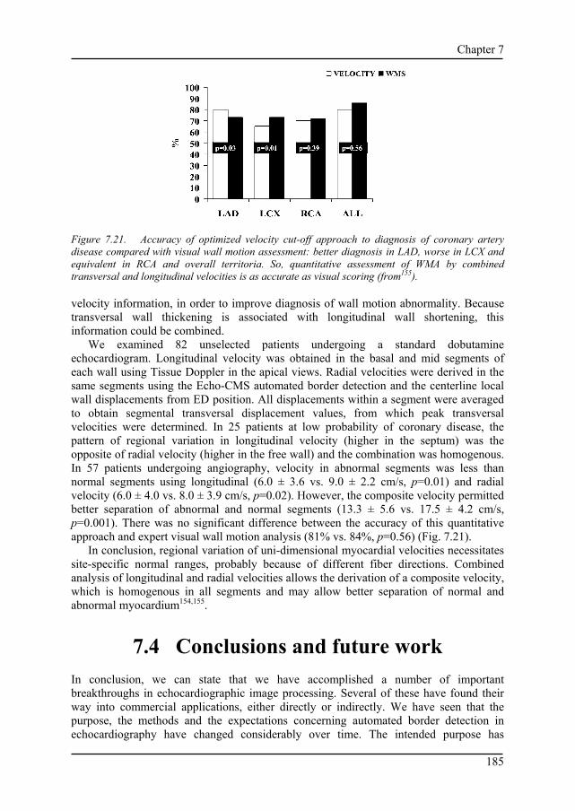
Chapter 7

185

Figure 7.21. Accuracy of optimized velocity cut-off approach to diagnosis of coronary artery disease compared with visual wall motion assessment: better diagnosis in LAD, worse in LCX and equivalent in RCA and overall territoria. So, quantitative assessment of WMA by combined transversal and longitudinal velocities is as accurate as visual scoring (from155). velocity information, in order to improve diagnosis of wall motion abnormality. Because transversal wall thickening is associated with longitudinal wall shortening, this information could be combined.

We examined 82 unselected patients undergoing a standard dobutamine echocardiogram. Longitudinal velocity was obtained in the basal and mid segments of each wall using Tissue Doppler in the apical views. Radial velocities were derived in the same segments using the Echo-CMS automated border detection and the centerline local wall displacements from ED position. All displacements within a segment were averaged to obtain segmental transversal displacement values, from which peak transversal velocities were determined. In 25 patients at low probability of coronary disease, the pattern of regional variation in longitudinal velocity (higher in the septum) was the opposite of radial velocity (higher in the free wall) and the combination was homogenous. In 57 patients undergoing angiography, velocity in abnormal segments was less than normal segments using longitudinal (6.0 ± 3.6 vs. 9.0 ± 2.2 cm/s, p=0.01) and radial velocity (6.0 ± 4.0 vs. 8.0 ± 3.9 cm/s, p=0.02). However, the composite velocity permitted better separation of abnormal and normal segments (13.3 ± 5.6 vs. 17.5 ± 4.2 cm/s, p=0.001). There was no significant difference between the accuracy of this quantitative approach and expert visual wall motion analysis (81% vs. 84%, p=0.56) (Fig. 7.21).

In conclusion, regional variation of uni-dimensional myocardial velocities necessitates site-specific normal ranges, probably because of different fiber directions. Combined analysis of longitudinal and radial velocities allows the derivation of a composite velocity, which is homogenous in all segments and may allow better separation of normal and abnormal myocardium154,155.

7.4 Conclusions and future work In conclusion, we can state that we have accomplished a number of important breakthroughs in echocardiographic image processing. Several of these have found their way into commercial applications, either directly or indirectly. We have seen that the purpose, the methods and the expectations concerning automated border detection in echocardiography have changed considerably over time. The intended purpose has

Chapter 7

186

evolved from automated TEE monitoring of cardiac function, via automatic LV volume measurements towards detection and classification of wall motion abnormalities, and is now shifting to 3D and 4D echocardiography. The applied methods changed from low-level bottom-up edge finding and linking into medium-level pattern matching and sequence tracking approaches (MCCT), further into complex geometrical and statistical models (AAM), and finally are moving into the realm of artificial intelligence (agent-based approaches). The expectations have become more realistic over the years, but at the same time the requirements have increased – from detection of a simple global measure to the classification of abnormal motion patterns over all regions of the LV, and from finding a single contour in a single frame to full-cycle detection of borders in all cardiac cycles and all angles of a 4D image set. We hope to have shown that we have made important contributions to this field of research. Furthermore, our research has spawned a wide array of secondary developments that made it into the literature and/or into commercial applications. Also, many researchers have extended our methods and applied them with success.

7.4.1 Outcome of earlier predictions In the previous chapters, we have made several predictions on the future of ultrasound and echocardiographic image processing. Some of these already have come true:

• With improvement of image quality, real-time 3D ultrasound may become an important substrate for ABD (Ch. 1). The Philips Live3D approach and its on-board semiautomatic detection156 are the first realization of this; other vendors are following rapidly.

• The next-generation ABD technique for ultrasound may well emerge from the family of appearance models (Ch. 1). Several vendors are currently investigating such techniques72,157.

In 1987, our work started, aiming at fully automated border detection in TEE for monitoring of cardiac function. In that year, Charles Lancée, who pioneered some of this work1 formulated the following proposition (‘stelling’) in his Ph.D. thesis:

“Fully automated border detection and the resulting quantitative monitoring of left ventricular geometry is still in its infancy, for the time being.”

We must conclude that this was indeed very true, and that the problem of fully automated echocardiographic border detection suitable for monitoring, after 20 years, is actually still in its childhood, or maybe in its adolescence.

Actually, considering the amount of research that has been spent worldwide on automated analyses for ultrasound images, and the hundreds of methods that have been described in literature, it is surprising how little automatic border detection has penetrated clinical practice. Some systems are available, some ultrasound manufacturers have included methods in their equipment, but grosso modo ultrasound remains a modality that is visually interpreted or manually analyzed.

In our opinion, the conclusion should be that the difficulty of the task was grossly misapprehended. The same applies to similar tasks such as (continuous, speaker-independent) speech recognition, identification of faces (under non-controlled circumstances) etc. Aside from some controlled, special applications, these are still largely unsolved problems, despite decades of intense research. Because we humans perform such

Chapter 7

187

tasks constantly and without effort, it is very hard for us to acknowledge that the mechanisms for doing this are in fact extremely complex. However, slowly we learn more and more about these mechanisms, computers become more powerful and undoubtedly a solution will become available at some point.

7.4.2 General future of echocardiographic imaging and image processing

Currently, we foresee a number of developments in echocardiography and image processing.

7.4.2.1 From 2D to 3D. 3D will become the standard modality in ultrasound imaging. This will be the case for TTE, TEE, intraoperative, intracardiac, and intravascular imaging. This will also happen for non-cardiological ultrasound, e.g. for peripheral or ob/gyn use. With the further evolution of transducers and front-end acquisition hardware, the majority of transducers will be principally real-time 3D, removing most limitations posed by 2D planes. Improved stereoscopic displays may eliminate much of the current visualization limitations. Anatomic B-mode or anyplane images may replace the current 2D functionality, just like (anatomic) M-mode imaging is nowadays a functional subset of B-mode imaging. Combined with integrated probe position sensing, freehand probe manipulation will allow acquisition of large 3D volumes (e.g. trajectories of long vessels) by volume stitching techniques.

7.4.2.2 Combination of diagnostic and therapeutic use of ultrasound. Especially the developments in ultrasound contrast agents will allow ultrasound to be used simultaneously for diagnosis and therapy. The microscopic gas bubbles are strong ultrasound reflectors and are very well visible in the echogram. This allows the use of contrast for blood opacification and myocardial perfusion visualization. Also, specialized contrast agents could be developed for functional imaging of pressure, temperature etc.

Contrast bubbles can also be manipulated or destroyed by high-energy pulses of ultrasound. This allows the creation of ‘smart bubbles’ for drug and gene delivery and targeted imaging; in the shell (or inside) of such bubbles, special ligands, drugs or genes are incorporated that can be released at a specific site by destroying the bubbles with ultrasound. These new applications of contrast agents can potentially have an enormous clinical impact and will require new echocardiographic quantification tools as well as allow new forms of parametric imaging.

7.4.2.3 Integration of image analysis in front-end processing Advances in computing power will allow to make the ultrasound front-end more intelligent. E.g. image acquisition settings may be optimized on-line (e.g. by automatically adjusting depth-gain or lateral gain settings, suppression of near-field artifacts and other anomalies, etc. Furthermore, the signal acquisition may be optimized with knowledge of the image content, derived from a previous analysis or segmentation. (Naturally, this should be applied with care in ambiguous situations; the hypothesis may amplify itself at

Chapter 7

188

the cost of other viable interpretations.) Such developments may improve image quality and benefit image segmentation.

7.4.2.4 Portability and automation. Ultrasound equipment will become more and more miniaturized, and will become available in very portable form (laptops, handhelds). Meanwhile, all functionality of current high-end machines will also be available in small formats and at low cost. More and more, imaging settings will be automatically optimized. This will also allow a more widespread use of ultrasound (by less experienced physicians) and will induce a need for more objective, automated analysis approaches.

7.4.2.5 Better modeling of organs in context We have made significant steps towards better modeling of the left ventricle, resulting in improved analyses; however, much remains to be gained in this terrain. In an ideal model, dynamic and functional aspects of the organ in its neighborhood should be included, as well as natural variation, congenital abnormalities, and pathological changes. Apart from the shape of the organ, its appearance in the ultrasound image and its typical artifacts should be modeled as well. If appearance for multiple modalities (ultrasound, MR, CT, different machines or acquisition protocols) can be modeled in conjunction, this would form the key to intermodality registration.

Such an ideal model will require significant advances in geometric modeling and combinations with statistical shape/appearance modeling, medical knowledge engineering etc. If such a model can be realized, it will not only allow improved segmentation, but also open the way to more advanced computer aided diagnosis: the diagnosis that best predicts (or matches) the currently derived images/segmentation (given all non-image based patient knowledge) would be considered correct.

7.4.2.6 Multimodal integration (MR, CT, X-ray, ultrasound) Especially for interventions, it is often desirable to combine the advantages of different imaging modalities. The detailed, high-quality anatomical 3D information from a preoperative MR or CT can then be combined with real-time, intraoperative ultrasound information. With the use of position sensing, anatomical landmarks or intermodality registration techniques, it should be possible in these different modalities to align coordinate systems, and apply the same anatomical models for segmentation (see previous point). This is a research area of growing interest, not only in fields like neurosurgery, but also in cardiology, e.g. for electrophysiology interventions, ASD/VSD closures etc.

7.4.2.7 Further miniaturization Unlike MR or CT, ultrasound image generation does not require high-energy elements or enclosure of the body; miniaturization is limited mainly by the state of the art in microchip technology, especially micromachining. Therefore, ultrasound can evolve into an extremely ‘miniaturized’ modality, even beyond handheld devices: its functionality can in principle migrate down to a microscale. Ultrasound imaging can reach much higher resolutions (at the cost of limited penetration) by using higher frequencies. Also, latency between image formation and display can be very small, allowing real-time, very high frame-rate imaging. Ultrasound in the future is likely to be used for real-time, direct local

Chapter 7

189

inspection of (dynamic) organs, probably within a larger anatomic framework put up by MR or CT (see above). This makes it very useful for catheter-tip interventional use, especially in combination with position sensing and precise stereotactic catheter steering, and possibly for freely navigating microscale or nanoscale devices.

Acknowledgements We gratefully acknowledge the financial support of the organizations and companies mentioned in this chapter, as well as the efforts of the many researchers and physicians who contributed to the different studies described here.

References 1. Lancée CT. A transesophageal phased array transducer for ultrasonic imaging of the heart. (PhD thesis).

Rotterdam, the Netherlands: Erasmus University Rotterdam; 1987. 2. Jenkins JM, Qian G, Besozzi M, Delp EJ, Buda AJ. Computer processing of echocardiographic images for

automated edge detection of left ventricular boundaries. In: Computers in Cardiology; 1981: IEEE Computer Society Press; p. 391-394.

3. Linker DT, Pearlman AS, Lewellen TK, Huntsman LH, Moritz WE. Automated endocardial definition of 2-D echocardiograms: a comparison of four standard edge detectors and improved thresholding techniques. In: Computers in Cardiology; 1982: IEEE Computer Society Press; p. 395-398.

4. Zwehl W, Levy R, Garcia EV, Haenchen RV, Childs W, Corday SR, Meerbaum S, Corday E. Validation of computerized edge detection algorithm for qualitative 2-D echocardiography. Circulation 1983;68:1127-1135.

5. Lancée CT, Rijsterborgh H, Bom N. Monitoring aspects of an ultrasonic esophageal transducer. Medical Progress through Technology 1988;13:131-138.

6. Grube E, Mathers F, Backs B, Luederitz B. Automatische und halbautomatische Konturfindung des linken Ventrikels im zweidimensionalen Echokardiogramm. In-vitro Untersuchungen an formalinfixierten Schweineherzen. Z Kardiol 1985;74(1):15-22.

7. Reiber JHC, Serruys PW, Kooijman CJ, Wijns W, Slager CJ, Gerbrands JJ, Schuurbiers JCH, den Boer A, Hugenholtz PG. Assessment of short-, medium-, and long-term variations in arterial dimensions from computer-assisted quantitation of coronary cineangiograms. Circulation 1985;71:280-288.

8. van Leeuwen PJ, Reiber JHC. Automated detection of left ventricular boundaries from 35mm contrast cineangiograms. In: Young IT, Biemond J, et al., eds. Signal Processing III: theories and applications, Eusipco-86; 1986; Amsterdam: North-Holland; p. 1409-1412.

9. van Daele M, Bosch HG, Reiber H, Sutherland GR, Roelandt JRTC. Can changes in cardiac output during surgery be monitored by transesophageal echo and computer-assisted analysis? Int J Cardiac Imaging 1989;4(1):70.

10. van Daele M, Bosch HG, Reiber H, Sutherland GR, Roelandt JRTC. Monitoring changes in cardiac output by transesophageal echo and computer-supported analysis: is it feasible? Eur Heart J 1989;10(Suppl):179.

11. Bosch JG, Reiber JHC, van Burken G, Gerbrands JJ, Gussenhoven EJ, Roelandt JRTC. Quantitative esophageal short-axis echocardiography with automatic endocardial contour detection. Eur Heart J 1988;9(Suppl 1):378.

12. Bosch JG, Reiber JHC, van Burken G, Gerbrands JJ, Gussenhoven EJ, Bom N, Roelandt JRTC. Automated endocardial contour detection in short-axis 2-D echocardiograms: methodology and assessment of variability. In: Ripley KL, ed. Computers in Cardiology; 1988; Washington DC: IEEE Computer Society; p. 137-140.

13. Bosch HG, Reiber JHC, van Burken G, Gerbrands JJ, Roelandt JRTC. Automated contour detection on short-axis transesophageal echocardiograms. In: Erbel R, Khanderia BK, et al., editors. Transesophageal Echocardiography A new window to the heart. Berlin: Springer; 1988. p. 253-259.

14. Bosch JG, Reiber JHC, van Burken G, Gerbrands JJ, Gussenhoven WJ, Bom N, Roelandt JRTC. Automated contour detection on short-axis echocardiograms. In: 8th int symp Echocardiology; 1989; Rotterdam; p. 77.

Chapter 7

190

15. Bosch JG, Reiber JHC, van Burken G, Gerbrands JJ, van Daele MERM, Roelandt JRTC. Automated endocardial contour detection on short-axis TEE echocardiograms. In: Abstract book Symposium Slokdarm Echocardiografie, 26 januari 1990, Academisch Medisch Centrum, Amsterdam; 1990. p. 18.

16. Ezekiel A, Garcia EV, Areeda JS, Corday SR. Automatic and intelligent left ventricular contour detection from two-dimensional echocardiograms. In: Ripley K, ed. Computers in Cardiology; 1984; Linkoping, Sweden: IEEE Computer Society Press; p. 261-264.

17. Klingler JW, Vaughan CL, Fraker TD, Andrews LT. Segmentation of echocardiographic images using mathematical morphology. IEEE Trans Biomed Eng 1988;35:925-934.

18. Friedland N, Adam D. Echocardiographic myocardial edge detection using an optimization protocol. In: Ripley K, ed. Computers in Cardiology; 1989; Los Alamitos, CA: IEEE Computer Society Press; p. 379-382.

19. Cohen LD. Note on active contour models and balloons. CVGIP Image Understanding 1991;53:211-218. 20. Bosch JG, Reiber JHC, van Burken G, Gerbrands JJ, Kostov A, van de Goor AJ, van Daele MERM,

Roelandt JRTC. Developments towards real-time frame-to-frame automatic contour detection in echocardiograms. In: Ripley KL, ed. Computers in Cardiol; 1990; Chicago: IEEE Computer Society Press; p. 435-438.

21. von Land CD, Rao SR, Reiber JHC. Implementing the centreline wall motion model with CLAS. In: Murray A, Ripley K, eds. Computers in Cardiology; 1990; Chicago: IEEE Computer Society Press; p. 687-690.

22. Gussenhoven EJ, Essed CE, Lancée CT, Mastik F, Frietman P, van Egmond FC, Reiber JHC, Bosch JG, van Urk H, et al. Arterial wall characteristics determined by intravascular ultrasound imaging: an in vitro study. J Am Coll Cardiol 1989;14(4):947-952.

23. Bom N, ten Hoff H, Lancée CT, Gussenhoven WJ, Bosch JG. Early and recent intraluminal ultrasound devices. Int J Cardiac Imaging 1989;4:79-88.

24. Bom N, Bosch JG, Reiber JHC, Gussenhoven EJ, Slager CJ, Brower RW. Current intra-arterial ultrasound imaging systems and automatic contour detection. In: Reiber JHC, Serruys PW, editors. Quantitative Coronary Arteriography. Dordrecht: Kluwer; 1990. p. 199-210.

25. Bom N, Reiber JHC, Lancée CT, Bosch JG, Roelandt JRTC, Lachmann B. Technik für intraluminales Monitoring von Herz und Blutgefäßen mit Ultraschall. In: Versprille A, editor. Monitoring. Berlin: Springer; 1992. p. 45-54.

26. van der Geest RJ, Jansen E, Buller VGM, Reiber JHC. Automated detection of left ventricular epi- and endocardial contours in short-axis MR images. In: Computers in Cardiology; 1994; Bethesda, MD: IEEE Computer Society Press; p. 33-36.

27. Bot H, Delemarre BJ, Bosch JG, Visser CA. Automation in echocardiography. Neth J Cardiol 1993;3:161-167.

28. Reiber JHC, van der Zwet PMJ, von Land CD, Koning G, Bosch JG, van der Geest RJ. New developments in cardiovascular image processing applications. In: Mortier E, Poelaert J, editors. Update in cardiac surgery, anesthesia and intensive care. Ghent; 1993. p. 113-114.

29. Bosch JG, Savalle LH, van Burken G, Reiber JHC. Evaluation of a semiautomatic contour detection approach in sequences of short-axis two-dimensional echocardiographic images. J Am Soc Echocardiogr 1995;8(6):810-821.

30. Bosch JG, van Burken G, Savalle LH, Reiber JHC. Automated endocardial border detection in sequences of echocardiograms. J Am Soc Echocardiogr 1994;3(part 2 supplement):S39.

31. Bosch JG, Reiber JHC, van Burken G, Savalle LH. Automated endocardial border detection in sequences of echocardiograms. In: 61 Jahrestagung der Deutschen Gesellschaft für Kardiologie - Herz- und Kreislaufforschung; 1995; Mannheim; p. Abstract 184.

32. Reiber JHC, Bosch JG, van Burken G, Savalle LH. Automatic contour detection in two-dimensional echocardiographic sequences. In: Abstract book 11th Symp on Echocardiology; 1995; Rotterdam; p. 176.

33. Blankenburgh R. Contourdetectie in echocardiogrammen. Detectie van de endocardiale contour van het linkerventrikel in series echocardiografische vierkamerdoorsneden. (MSc Thesis). Delft: Delft University of Technology; 1994.

34. Picard MH, Bosch HG, Morrissey RL, Reiber JHC. Automated echocardiographic ventricular volume quantitation - validation of a new border detection method. Circulation 1994;90(4 Suppl):I-608.

35. Reiber JHC, Goedhart B, Bosch HG, van der Geest RJ, Dijkstra J, Koning G, Ramze Rezaee M, Lelieveldt BPF, de Roos A, et al. Quantitative cardiovascular image analysis: current status and what are realistic expectations for the future? In: van der Wall EE, Manger Cats V, et al., editors. Vascular Medicine From Endothelium to Myocardium. Dordrecht: Kluwer; 1997. p. 103-131.

36. van Dantzig JM, Bosch HG, Cheriex EC, Wellens HJ. Automatic left ventricular wall motion scoring by an endocardial contour detection system. In: 69th scientific sessions American Heart Association; 1996; p. (unpublished).

Chapter 7

191

37. Bosch JG, van Burken G, Reiber JHC. Automated frame-to-frame contour detection in echocardiograms using motion estimation. In: Murray A, ed. Computers in Cardiol; 1992; Durham, NC: IEEE Computer Society Press; p. 351-354.

38. Bosch JG, van Burken G, Reiber JHC. Automatic frame-to-frame contour detection in echocardiograms using motion estimation. In: Abstract book 10th Symp on Echocardiology; 1993 June 23-25, 1993; Rotterdam; p. 165.

39. Maliepaard C. Blockmatching in echocardiografische beelden. (MSc Thesis). Delft: Delft University of Technology; 1996.

40. Perez JE, Waggoner AD, Barzilai B, Melton HE, Miller JG, Sobel BE. On-line assessment of ventricular function by automatic boundary detection and ultrasonic backscatter imaging. J Am Coll Cardiol 1992;19(2):313-320.

41. Smith MD, Xie GY, Sapin PM. Factors affecting the determination of left ventricular area by acoustic quantification. J Am Coll Cardiol 1992;19:299A.

42. Bosch JG, Reiber JHC, van Burken G, Savalle LH, Maurincomme E, Helbing WA. Automated contour detection and acoustic quantification. Eur Heart J 1995;16(Suppl J):35-41.

43. Bosch JG, van Burken G, Schukking SS, Wolff R, van de Goor AJ, Reiber JHC. Real-time frame-to-frame automatic contour detection on echocardiograms. In: Murray A, ed. Computers in Cardiol; 1994; Bethesda, MD: IEEE Computer Society Press; p. 29-32.

44. Lang RM, Vignon P, Weinert L, Bednarz J, Korcarz C, Sandelski J, Koch R, Prater D, Mor-Avi V. Echocardiographic quantification of regional left ventricular wall motion with color kinesis. Circulation 1996;93(10):1877-1885.

45. Bosch HG, van Burken G, Nijland F, Reiber JHC. Overview of automated quantitation techniques in 2D echocardiography. In: Reiber JHC, van der Wall EE, editors. What's new in cardiovascular imaging. Dordrecht, the Netherlands: Kluwer; 1998. p. 363-376.

46. Bosch JG, Nijland F, van Burken G, Reiber JHC. Feasibility of model-based automated border detection for quantification of stress echocardiography. In: Abstract book 13th Symp on Echocardiology; 1999; Rotterdam; p. 70.

47. Bosch JG, Mitchell SC, Lelieveldt BPF, Sonka M, Nijland F, Reiber JHC. Model-based automated border detection for quantitative stress echocardiography. Eur Heart J 2000;21(abstract suppl):37.

48. Bosch JG, Reiber JHC. Two-dimensional echocardiographic digital image processing and approaches to endocardial edge detection. In: Otto CM, editor. The practice of clinical echocardiography. Second ed. Orlando, FL: W.B. Saunders; 2002. p. 141-158.

49. Nijland F, Kamp O, Verhorst PMJ, de Voogt WG, Visser CA. Early prediction of improvement in ejection fraction after acute myocardial infarction using low dose dobutamine echocardiography. Heart 2002;88:592-596.

50. Nijland F, Kamp O, Verhorst PMJ, de Voogt WG, Bosch HG, Visser CA. Myocardial viability: impact on left ventricular dilatation after acute myocardial infarction. Cardiologie 1997;4:483.

51. Nijland F, Kamp O, Verhorst PMJ, de Voogt WG, Bosch HG, Visser CA. Impact of myocardial viability on left ventricular dilatation following acute myocardial infarction. J Am Coll Cardiol 1998;31(2 suppl A):408A.

52. Nijland F, Kamp O, Verhorst PMJ, de Voogt WG, Bosch HG, Visser CA. Myocardial viability: impact on left ventricular dilatation after acute myocardial infarction. Heart 2002;87(1):17-22.

53. Fry SJ, Hunziker PR, Bosch HG, Reiber JHC, Picard MH. Automated echocardiographic confirmation of regional wall motion abnormalities: quantitation of continuous LV volume. J Am Coll Cardiol 1998;31(2 suppl. A):56A.

54. Fry SJ, Hunziker PR, Bosch JG, Reiber JHC, Morrissey RL, Picard MH. Temporal characteristics of left ventricular systolic volume in ischemic heart disease: an automated border detection study. unpublished 2000.

55. Schöb L, Hunziker PR, Bosch HG, Füllhaas U, Hess N, Pfisterer M, Buser P. Automatic border detection zur Quantifizierung der Wandmotilität in der Stressechokardiographie. Kardiovaskuläre Medizin 1999;2(Suppl 1):19S.

56. Hunziker PR, Schöb L, Bosch HG, Hess N, Kaiser C, Pfisterer M, Buser P. Quantitative dobutamine stress echocardiography: new insights with automatic border detection. J Am Soc Echocardiogr 1999;12(5):386.

57. Hunziker PR, Schöb L, Lefkovits M, Füllhaas U, Yoon SI, Bosch HG, Cron T, Pfisterer M, Buser P. Automatic border detection in dobutamine stress echo: how do normal and ischaemic segments behave objectively and quantitatively? Eur Heart J 1999;20(abstract suppl):618.

58. Hunziker PR, Yuan D, Schöb L, Bosch HG, Pfisterer M, Buser P. Objective and quantitative stress echo analysis to diagnose coronary disease using model-based image processing. J Am Coll Cardiol 2000;35(2 suppl A):431A.

Chapter 7

192

59. Hunziker PR, Yuan D, Schöb L, Jansen C, Bosch JG, Marsch S, Pfisterer M. Computer vision for objective and quantitative analysis of stress echocardiograms. unpublished 2002.

60. Marwick TH. Stress echocardiography: its role in the diagnosis and evaluation of coronary artery disease. 1st ed. Dordrecht: Kluwer; 1994.

61. Biagini E, Elhendy A, Bax JJ, Schinkel AFL, Poldermans D. The use of stress echocardiography for prognostication in coronary artery disease: an overview. Curr Opin Cardiol 2005;20(5):386-394.

62. Marwick TH. Stress echocardiography with nonexercise techniques. Principles, protocols, interpretation, and clinical applications. In: Otto CM, editor. Clinical echocardiography. 2nd ed. Philadelphia: Saunders; 2002. p. 301-339.

63. Hoffmann R, Lethen H, Marwick TH, Arnese M, Fioretti P, Pingitore A, Picano E, Buck T, Erbel R, et al. Analysis of interinstitutional observer agreement in interpretation of dobutamine stress echocardiograms. J Am Coll Cardiol 1996;27(2):330-336.

64. Marwick TH. Quantitative techniques for stres echocardiography:dream or reality? Eur J Echocardiography 2002;3(3):171-176.

65. Oost CR, Koning G, Sonka M, Reiber JHC, Lelieveldt BPF. Automated segmentation of x-ray left ventricular angiograms using multi-view active appearance models. In: Frangi AF, Radeva PI, et al., eds. Functional Imaging and Modeling of the Heart, Proc 3rd Int Workshop FIMH 2005, LNCS 3504; 2005; Barcelona: Springer; p. 23-32.

66. Üzümcü M, van der Geest RJ, Sonka M, Lamb HJ, Reiber JHC, Lelieveldt BPF. Multiview active appearance models for simultaneous segmentation of cardiac 2- and 4-chamber long-axis magnetic resonance images. Invest Radiol 2005;40(4):195-203.

67. van Assen HC, Danilouchkine MG, Frangi AF, Ordas S, Westenberg JJM, Reiber JHC, Lelieveldt BPF. SPASM: Segmentation of sparse and arbitrarily oriented cardiac MRI data using a 3D ASM. In: Frangi AF, Radeva PI, et al., eds. Functional Imaging and Modeling of the Heart, Proc 3rd Int Workshop FIMH 2005, LNCS 3504; 2005; Barcelona: Springer; p. 33-43.

68. van der Geest RJ, Lelieveldt BPF, Angelié E, Danilouchkine MG, Sonka M, Reiber JHC. Evaluation of a new method for automated detection of left ventricular contours in time series of magnetic resonance images using an active appearance motion model. J Cardiovasc Magn Reson 2004;6(3):609-617.

69. Beichel R, Gotschuli G, Sorantin E, Leberl F, Sonka M. Diaphragm dome surface segmentation in CT data sets: a 3D active appearance model approach. In: Sonka M, Fitzpatrick JM, eds. SPIE Medical Imaging: Image Processing, vol 4684; 2002; San Diego: SPIE; p. 475-484.

70. Beichel R, Mitchell SC, Sorantin E, Leberl F, Goshtasby A, Sonka M. Shape- and appearance-based segmentation of volumetric medical images. In: Proc ICIP 2001; 2001; Los Alamitos, CA: IEEE; p. 589-592.

71. Chatelet G. Étude et réalisation d'une méthode de segmentation adaptée aux échocardiographies. (MSc Thesis). Caen: University of Caen; 2003.

72. Hansegard J, Urheim S, Steen E, Torp H, Olstad B, Malm S, Rabben SI. Detection of the myocardial boundary in the left ventricle from simultaneously acquired triplane ultrasound images using multi view active appearance motion models. In: IEEE Int Ultrasonics Symp; 2005; Rotterdam: IEEE; p. 2267-2270.

73. Cootes TF, Edwards GJ, Taylor CJ. Active Appearance Models. In: Burkhardt H, Neumann B, eds. European Conf Computer Vision; 1998; Berlin: Springer; p. 484-498.

74. Lelieveldt BPF, van der Geest RJ, Mitchell SC, Bosch JG, Sonka M, Reiber JHC. Automated model-based segmentation of the right and left ventricular contours. Eur Heart J 2000;21(abstract suppl):582.

75. Bosch JG, Mitchell SC, Lelieveldt BPF, Sonka M, Nijland F, van Burken G, Reiber JHC. Feasibility of fully automated border detection on stress echocardiograms by Active Appearance Models. Eur Heart J 2000;21(abstract suppl):11.

76. Bosch HG, Mitchell SC, Lelieveldt BPF, Sonka M, Nijland F, Reiber JHC. Feasibility of fully automated border detection on stress echocardiograms by active appearance models. Circulation 2000;102(18 Suppl II):633.

77. Bosch JG, Mitchell SC, Lelieveldt BPF, Sonka M, Nijland F, Kamp O, Reiber JHC. Fully automated border detection for stress echo by Active Appearance Models. Eur J Echocardiography 2000;1(suppl. 2):S34.

78. Mitchell SC, Lelieveldt BPF, van der Geest RJ, Bosch HG, Reiber JHC, Sonka M. Multistage hybrid active appearance model matching: Segmentation of left and right ventricles in cardiac MR images. IEEE Trans Med Imaging 2001;20(5):415-423.

79. Bosch HG, Mitchell SC, Lelieveldt BPF, Nijland F, Kamp O, Sonka M, Reiber JHC. Active Appearance Motion Models for endocardial contour detection in time sequences of echocardiograms. In: Sonka M, Hanson KM, eds. SPIE Medical Imaging: Image Processing, vol 4322; 2001; San Diego: SPIE; p. 257-268.

80. Mitchell SC, Lelieveldt BPF, van der Geest RJ, Bosch HG, Reiber JHC, Sonka M. Time continuous segmentation of cardiac MR image sequences using active appearance motion models. In: Sonka M,

Chapter 7

193

Hanson KM, eds. SPIE Medical Imaging: Image Processing, vol 4322; 2001; San Diego: SPIE; p. 249-256.

81. Sonka M, Lelieveldt BPF, Mitchell SC, Bosch HG, van der Geest RJ, Reiber JHC. Active appearance motion model segmentation. In: 2nd int workshop Digital and Computational Video; 2001; Tampa, FL: IEEE Computer Society; p. 64-68.

82. Lelieveldt BPF, Mitchell SC, Bosch JG, van der Geest RJ, Sonka M, Reiber JHC. Time-continuous segmentation of cardiac image sequences using Active Appearance Motion Models. In: Insana MF, Leahy RM, eds. Information Processing in Medical Imaging (IPMI), LNCS2082; 2001; Davis, CA: Springer; p. 446-452.

83. Bosch HG, Mitchell SC, Lelieveldt BPF, Nijland F, Kamp O, Sonka M, Reiber JHC. Active Appearance-Motion Models for fully automated endocardial contour detection in time sequences of echocardiograms. In: Lemke HU, Vannier MW, et al., eds. Computer Assisted Radiology and Surgery (CARS), ICS1230; 2001; Berlin: Elsevier; p. 896-901.

84. Bosch JG, Mitchell SC, Lelieveldt BPF, Nijland F, Kamp O, Sonka M, Reiber JHC. Fully automated endocardial contour detection in time sequences of echocardiograms by Active Appearance-Motion Models. In: Computers in Cardiology, vol 28; 2001; Rotterdam; p. 93-96.

85. Bosch JG, Mitchell SC, Lelieveldt BPF, Nijland F, Kamp O, Sonka M, Reiber JHC. Fully automated endocardial border detection in sequences of echocardiograms by active appearance-motion models. Circulation 2001;104(17 suppl II):652.

86. Bosch JG, Mitchell SC, Lelieveldt BPF, Nijland F, Kamp O, Sonka M, Reiber JHC. Automatic segmentation of echocardiographic sequences by active appearance motion models. IEEE Trans Med Imaging 2002;21(11):1374-1383.

87. Lelieveldt BPF, Mitchell SC, van der Geest RJ, Bosch HG, Sonka M, Reiber JHC. Time continuous segmentation of cardiac MR images using Active Appearance Motion Models. In: Lemke HU, Vannier MW, et al., eds. Computer Assisted Radiology and Surgery (CARS), ICS1230; 2001; Berlin: Elsevier; p. 917-921.

88. Lelieveldt BPF, Mitchell SC, Bosch JG, Sonka M, Reiber JHC, van der Geest RJ. Time-continuous automated contour detection of the endo- and epicardium in short-axis cardiac MR image sequences. Eur Heart J 2001;22(abstract suppl ESC Stokholm):352.

89. Lelieveldt BPF, van der Geest RJ, Mitchell SC, Bosch JG, Sonka M, Reiber JHC. Fully automated, time-continuous contour delineation of the endo- and epicardium in short-axis cardiac MR image sequences. Proc Int Soc Mag Reson Med 2001;9:600.

90. Bosch JG, Mitchell SC, Lelieveldt BPF, Nijland F, Kamp O, Sonka M, Reiber JHC. Fully automated endocardial contour detection in time sequences of echocardiograms by three-dimensional Active Appearance Models. In: Sonka M, Fitzpatrick JM, eds. SPIE Medical Imaging: Image Processing, vol 4684; 2002; San Diego: SPIE; p. 452-462.

91. Mitchell SC, Lelieveldt BPF, Bosch JG, van der Geest RJ, Reiber JHC, Sonka M. Segmentation of cardiac MR volume data using 3D active appearance models. In: Sonka M, Fitzpatrick JM, eds. SPIE Medical Imaging: Image Processing, vol 4684; 2002; San Diego: SPIE; p. 433-443.

92. Lelieveldt BPF, Mitchell SC, Bosch JG, van der Geest RJ, Sonka M, Reiber JHC. 3D active appearance models: application to cardiac MR and ultrasound image segmentation. In: Lemke HU, Vannier MW, et al., eds. Computer Assisted Radiology and Surgery (CARS); 2002; Paris: Springer; p. 897-901.

93. Mitchell SC, Bosch JG, Lelieveldt BPF, van der Geest RJ, Reiber JHC, Sonka M. 3-D active appearance models: segmentation of cardiac MR and ultrasound images. IEEE Trans Med Imaging 2002;21(9):1167-1178.

94. Lelieveldt BPF, Mitchell SC, Bosch JG, van der Geest RJ, Sonka M, Reiber JHC. Automatic detection of endo- and epicardial contours in short-axis cardiac MR data using 3D active appearance models. JCMR 2002;4(1):106-107.

95. Bosch JG, Nijland F, Mitchell SC, Lelieveldt BPF, Kamp O, Sonka M, Reiber JHC. Automated classification of wall motion abnormalities by Principal Component Analysis of endocardial shape motion patterns in echocardiograms. In: Sonka M, Fitzpatrick JM, eds. SPIE Medical Imaging: Image Processing, vol 5032; 2003; San Diego: SPIE; p. 38-49.

96. Bosch JG, Nijland F, Mitchell SC, Lelieveldt BPF, Kamp O, Sonka M, Reiber JHC. Automated classification of wall motion abnormalities by analysis of left ventricular endocardial motion patterns. In: Abstract book Ned Ver v Cardiologie Scientific Meeting; 2003; Amsterdam; p. 125.

97. Bosch JG, Nijland F, Kamp O, van Burken G, Sonka M, Reiber JHC. Automated classification of wall motion abnormalities by automated border detection and analysis of left ventricular endocardial motion patterns. J Am Soc Echocardiogr 2003;16(5):507.

98. Sonka M, Bosch JG, Lelieveldt BPF, Mitchell SC, Reiber JHC. Computer-aided diagnosis via model-based shape analysis: cardiac MR and echo. In: Lemke HU, Vannier MW, et al., eds. Computer Assisted Radiology and Surgery (CARS), ICS1256; 2003; London: Esevier; p. 1013-1018.

Chapter 7

194

99. Bosch JG, Nijland F, Kamp O, van Burken G, Sonka M, Reiber JHC. Automated classification of wall motion abnormalities by analysis of left-ventricular endocardial motion patterns. Eur Heart J 2003;24(abstract suppl):203.

100. Bosch JG, Nijland F, Mitchell SC, Lelieveldt BPF, Kamp O, Sonka M, Reiber JHC. Automated classification of wall motion abnormalities by analysis of left ventricular endocardial contour motion patterns. Eur J Echocardiography 2003;4(suppl 1):S95.

101. Bosch JG, Nijland F, Mitchell SC, Lelieveldt BPF, Kamp O, Reiber JHC, Sonka M. Computer-aided diagnosis via model-based shape analysis: Automated classification of wall motion abnormalities in echocardiograms. Acad Radiol 2005;12(3):358-367.

102. Mitchell SC, Lelieveldt BPF, Bosch HG, Reiber JHC, Sonka M. Disease characterization of active appearance model coefficients. In: Sonka M, Fitzpatrick JM, eds. SPIE Medical Imaging: Image Processing, vol 5032; 2003; San Diego: SPIE; p. 949-957.

103. Üzümcü M, Frangi AF, Reiber JHC, Lelieveldt BPF. Independent component analysis in statistical shape models. In: SPIE Medical Imaging, Image Processing; 2003; San Diego, CA: SPIE; p. 375-383.

104. Suinesiaputra A, Üzümcü M, Frangi AF, Kaandorp TAM, Reiber JHC, Lelieveldt BPF. Detecting regional abnormal cardiac contraction in short-axis MR images using Independent Component Analysis. In: 7th int MICCAI conf, LNCS 3216; 2004: Springer; p. 737-744.

105. Gopal AS, Schnellbaecher MJ, Shen Z, Akinboboye OO, Sapin PM, King DL. Freehand three-dimensional echocardiography for measurement of left ventricular mass: in vivo anatomic validation using explanted human hearts. J Am Coll Cardiol 1997;30:802-810.

106. van Stralen M, Bosch JG, Voormolen MM, van Burken G, Krenning BJ, Lancée CT, de Jong N, Reiber JHC. A semi-automatic endocardial border detection method for the left ventricle in 4D ultrasound data sets. In: Lemke HU, Vannier MW, et al., eds. Computer Assisted Radiology and Surgery (CARS), ICS1268; 2003; Chicago: Esevier; p. 1078-1083.

107. van Stralen M, Bosch JG, Voormolen MM, van Burken G, Krenning BJ, Lancée CT, de Jong N, Reiber JHC. A semi-automatic endocardial border detection method for 4D ultrasound data. Medical Image Computing and Computer-Assisted Intervention - MICCAI 2004, Pt 1, LNCS3216 2004;LNCS3216:43-50.

108. van Stralen M, Bosch JG, Voormolen MM, van Burken G, Krenning BJ, van Geuns RJM, Lancée CT, de Jong N, Reiber JHC. Semi-automatic left ventricular endocardial border detection method for 4D ultrasound data. Eur J Echocardiography 2004;5(suppl 1):S57.

109. van Stralen M, Bosch JG, Voormolen MM, van Burken G, Krenning BJ, van Geuns RJM, Angelié E, Lancée CT, de Jong N, et al. Semi-automatic border detection method for left ventricular volume estimation in 4D ultrasound data. In: 11th ASCI conf; 2005; Heijen, NL; p. 200-207.

110. van Stralen M, Bosch JG, Voormolen MM, van Burken G, Krenning BJ, Lancée CT, de Jong N, Reiber JHC. Left ventricular volume estimation in cardiac 3D ultrasound: a semi-automatic border detection approach. Acad Radiol 2005;12:1241-1249.

111. van Stralen M, Bosch JG, Voormolen MM, van Burken G, Krenning BJ, van Geuns RJM, Angelie E, van der Geest RJ, Lancée CT, et al. Semi-automatic border detection method for left ventricular volume estimation in 4D ultrasound data. In: Fitzpatrick JM, ed. SPIE Medical Imaging - image processing vol 5747; 2005; San Diego, CA: SPIE, Bellingham, WA; p. 1457-1467.

112. van Stralen M, Voormolen MM, van Burken G, Krenning BJ, van Geuns RJM, Angelié E, van der Geest RJ, Lancée CT, de Jong N, et al. A novel dynamic programming based semi-automatic endocardial border detection method for 4D cardiac ultrasound. In: IEEE int Ultrasonics symp; 2005; Rotterdam; p. 1224-1227.

113. Bosch JG, van Stralen M, Voormolen MM, Krenning BJ, Lancée CT, Reiber JHC, van der Steen AFW, de Jong N. Improved spatiotemporal voxel space interpolation for 3D echocardiography with irregular sampling and multibeat fusion. In: IEEE int Ultrasonics symp; 2005; Rotterdam; p. 1232-1235.

114. Li W, Gussenhoven WJ, Bosch JG, Mastik F, Reiber JHC, Bom N. A computer-aided analysis system for the quantitative assessment of intravascular ultrasound images. In: Ripley KL, ed. Computers in Cardiol; 1990; Chicago: IEEE Computer Society Press; p. 333-336.

115. Li W, Bosch JG, Zhong Y, Gussenhoven WJ, Rijsterborgh H, Reiber JHC, Bom N. Semiautomatic frame-to-frame tracking of the luminal border from intravascular ultrasound. In: Murray A, ed. Computers in Cardiol; 1991; Venice, Italy: IEEE Computer Society Press; p. 353-356.

116. Li W, Bosch JG, Zhong Y, The SHK, Gussenhoven WJ, Mastik F, van Egmond FC, Rijsterborgh H, Reiber JHC, et al. Image segmentation and 3D reconstruction of intravascular ultrasound images. In: Wei Y, Gu B, editors. Acoustical imaging. New York: Plenum Press; 1992. p. 489-496.

117. Li W, The SHK, Wilson RA, Bosch JG, Gussenhoven EJ, Di Mario C, Reiber JHC, Bom N, Verdouw PD, et al. Semi-automatic frame-to-frame tracking of the luminal border from intravascular ultrasound: technical development and clinical applications. In: Li W, editor. Image and signal processing in intravascular ultrasound, PhD Thesis. Rotterdam: Erasmus University Rotterdam; 1997. p. 33-45.

Chapter 7

195

118. Li W, von Birgelen C, Hartlooper A, van der Lugt A, van Egmond FC, Di Mario C, Boersma E, van der Putten N, Bosch JG, et al. Three-dimensional reconstruction and volumetric quantification of intravascular ultrasound. In: Li W, editor. Image and signal processing in intravascular ultrasound, PhD Thesis. Rotterdam: Erasmus University Rotterdam; 1997. p. 47-67.

119. Maurincomme E. Analyse et segmentation d' images echographiques endovasculaires. (PhD Thesis). Lyon: Institut National des Sciences Appliques de Lyon (INSA); 1994.

120. Maurincomme E, Friboulet D, Finet G, Magnin I, Reiber JHC. ADDER: a snake-based segmentation approach for intravascular ultrasound images. In: Fung KK, Ginige A, eds. DICTA-93: Digital Image Computing: Techniques and Applications; 1993; Sydney, Australia: Australian Pattern Recognition Society; p. 422-429.

121. Dijkstra J, Wahle A, Koning G, Reiber JHC, Sonka M. Quantitative coronary ultrasound: state of the art. In: Reiber JHC, van der Wall EE, editors. What's new in Cardiovascular Imaging. Dordrecht: Kluwer Academic Publishers; 1998. p. 79-94.

122. Kostov A. Speeding up minimum cost contour detection. A status report. Delft, the Netherlands: Delft University of Technology; 1990.

123. Reiber JHC, Bosch JG, van Burken G. Automated Contour Detection - motivation and present state of the art. In: Abstract book 10th Symp Echocardiology. Rotterdam: Erasmus University Rotterdam; 1993. p. 115.

124. Reiber JHC, van der Zwet PMJ, Koning G, von Land CD, Bosch JG, Maurincomme E, van der Geest RJ, Gerbrands JJ. Perspectieven in beeldvorming en beeldverwerking. In: Verheugt FWA, Bos KW, editors. De toekomst van de cardiologie: Nederlandse Hartstichting; 1994. p. 63-91.

125. Kostov A. Video real-time minimum-cost contour detection (MSc Thesis). Delft: Delft University of Technology; 1991.

126. Schukking S. The minimum cost contour detector. Design and implementation of a high performance computation platform for real-time contour detection. (MSc Thesis). Delft: Delft University of Technology; 1992.

127. Salonen R, Salonen JT. Progression of carotid atherosclerosis and its determinants: a population based ultrasonography study. Atheroscler 1990;81:33-40.

128. Hoeks AP, Willekes C, Boutouyrie P, Brands PJ, Willigers JM, Reneman RS. Automated detection of local artery wall thickness based on M-line signal processing. Ultrasound Med Biol 1997;23(7):1017-1023.

129. Sonka M, Liang W, Lauer RM. Automated analysis of brachial ultrasound image sequences: Early detection of cardiovascular disease via surrogates of endothelial function. IEEE Trans Med Imaging 2002;21:1271-1279.

130. Sosef MN, Bosch JG, van Oostayen JA, Visser T, Reiber JHC, Rosendaal FR. Relation of plasma coagulation factor VII and fibrinogen to carotid artery intima-media thickness. Thromb Haemost 1994;72(2):250-254.

131. Šrámek A, Bosch JG, Reiber JHC, van Oostayen JA, Rosendaal FR. Ultrasound assessment of atherosclerotic vessel wall changes - Reproducibility of intima-media thickness measurements in carotid and femoral arteries. Invest Radiol 2000;35(12):699-706.

132. Helbing WA, Maliepaard C, Rebergen SA, Bosch HG, Ottenkamp J, de Roos A, Reiber JHC. Right ventricular function: assessment with echocardiography and correlation with magnetic resonance imaging. Cardiology in the Young 1994;4:22.

133. Helbing WA, Bosch HG, Maliepaard C, Rebergen SA, van der Geest RJ, Hansen B, Ottenkamp J, Reiber JHC, de Roos A. Comparison of echocardiographic methods with magnetic resonance imaging for assessment of right ventricular function in children. Am J Cardiol 1995;76(8):589-594.

134. Helbing WA, Maliepaard C, Bosch HG, Ottenkamp J, Reiber JHC. Echocardiographic quantification of right ventricular areas in children by automatic border detection. Eur Heart J 1994;15(abstract suppl):501.

135. Helbing WA, Maliepaard C, Bosch HG, de Roos A, Ottenkamp J, Reiber JHC. Automated border detection in echocardiographic quantification of right ventricular function in children: comparison with magnetic resonance imaging. Circulation 1995;92(8 Suppl I):I-442.

136. Helbing WA, Bosch HG, Maliepaard C, Zwinderman KH, Rebergen SA, Ottenkamp J, de Roos A, Reiber JHC. On-line automated border detection for echocardiographic quantification of right ventricular size and function in children. Pediatr Cardiol 1997;18(4):261-269.

137. Kamp O, Sieswerda GT, Visser CA. State-of-the-art. Stress echocardiography entering the next millennium. In: Reiber JHC, van der Wall EE, editors. What's new in cardiovascular imaging. Dordrecht, the Netherlands: Kluwer Academic Publishers; 1998. p. 351-362.

138. Warda HM, Bosch JG, Atsma DE, Jukema JW, van der Wall EE, Schalij MJ, Oemrawsingh PV. Intracoronary hyperbaric oxygen administered during primary percutaneous coronary intervention prevents one month left ventricular remodeling. Circulation 2004;110(17 suppl S):698.

Chapter 7

196

139. Warda HM, Bosch JG, Bax JJ, Atsma DE, Jukema JW, van der Wall EE, Schalij MJ, Oemrawsingh PV. Intracoronary hyperbaric oxygen administered during primary percutaneous coronary intervention prevents 1-month left ventricular remodeling. Am J Cardiol 2004;94(suppl 6A):89E.

140. Warda HM, Oemrawsingh PV, Atsma DE, Bosch JG, Lindsay BS, van der Wall EE, Schalij MJ. Perfusion recovery after myocardial infarction diagnostic (PYRAMID) score; first angiographic predictor of future left ventricular remodeling after acute myocardial infarction. Am J Cardiol 2004;94(suppl 6A):15E.

141. Warda HM, Bosch JG, Bax JJ, Atsma DE, Jukema JW, van der Wall EE, Schalij MJ, Oemrawsingh PV. Intracoronary hyperbaric oxygen administered during primary percutaneous coronary intervention prevents one month left ventricular remodeling. J Am Coll Cardiol 2005;45(3 suppl 1):242A.

142. Warda HM, Bax JJ, Bosch JG, Atsma DE, Jukema JW, van der Wall EE, van der Laarse A, Schalij MJ, Oemrawsingh PV. Effect of intracoronary aqueous oxygen on left ventricular remodeling after anterior wall ST-elevation acute myocardial infarction. Am J Cardiol 2005;96(1):22-24.

143. Buller VGM, Nyqvist C. The AiLV system: a pilot study in knowledge guided left ventricular angiographic image processing (MSc thesis). Leiden: University of Leiden; 1993.

144. Bovenkamp EGP, Dijkstra J, Bosch JG, Reiber JHC. Collaborative multi-agent IVUS image segmentation. Medical Image Computing and Computer-Assisted Intervention - MICCAI 2001, LNCS2208 2001:1185-1186.

145. Bovenkamp EGP, Dijkstra J, Bosch JG, Reiber JHC. Multi-agent IVUS image segmentation. In: Kröse B, de Rijke M, et al., eds. 13th Belgium-Netherlands Conference on Artificial Intelligence (BNAIC); 2001; Amsterdam: Amsterdam University Press; p. 357-364.

146. Bovenkamp EGP, Dijkstra J, Bosch JG, Reiber JHC. Multi-agent segmentation of IVUS images. Pattern Recognition 2004;37(4):647-663.

147. Bovenkamp EGP, Dijkstra J, Bosch JG, Reiber JHC. Multi-agent IVUS image interpretation. In: Sonka M, Fitzpatrick JM, eds. SPIE Medical Imaging: Image Processing, vol 5032; 2003; San Diego: SPIE; p. 619-630.

148. Bovenkamp EGP, Dijkstra J, Bosch JG, Reiber JHC. Multi-agent segmentation of IVUS images. In: Heskes T, Lucas P, et al., eds. 15th Belgium-Netherlands Conference on Artificial Intelligence (BNAIC); 2003; Nijmegen; p. 395-396.

149. Bovenkamp EGP, Dijkstra J, Bosch JG, Reiber JHC. User-agent cooperation in multi-agent IVUS image segmentation. IEEE Trans Med Imaging 2006:submitted.

150. Auricchio A, Ghanem A, Groethus F, Geller C, Nikutta P, Hartung W, Maarse A, Salo R, Spinelli J. Echocardiographic analysis of left ventricular contraction patterns in left bundle branch block and congestive heart failure. J Cardiac Failure 1999;5(3, suppl. 1):3.

151. Breithardt OA, Kramer AP, Schiffgens B, Franke A, Huvelle E, Auricchio A, Stellbrink C. Characteristics of left ventricular contraction patterns and acute changes with multisite pacing in patients with heart failure as assessed by echocardiographic semiautomatic contour detection. Eur Heart J 2000;21(Abstract suppl.):351.

152. Breithardt OA, Stellbrink C, Kramer AP, Sinha AM, Franke A, Salo R, Schiffgens B, Huvelle E, Auricchio A. Echocardiographic quantification of left ventricular asynchrony predicts an acute hemodynamic benefit of cardiac resynchronization therapy. J Am Coll Cardiol 2002;40(3):536-545.

153. Bax JJ, Ansalone G, Breithardt OA, Derumeaux G, Leclercq C, Schalij MJ, Sogaard P, St. John Sutton M, Nihoyannopoulos P. Echocardiographic evaluation of cardiac resynchronization therapy: ready for routine clinical use? A critical appraisal. J Am Coll Cardiol 2004;44(1):1-9.

154. Cain P, Short L, Marwick TH. Combination of long-axis and radial myocardial velocity offers a new quantitative parameter of regional ventricular function, independent of segment location. Circulation 2000;102(18 Suppl. II):II-382.

155. Cain P, Short L, Baglin T, Case C, Bosch HG, Marwick TH. Development of a fully quantitative approach to the interpretation of stress echocardiography using radial and longitudinal myocardial velocities. J Am Soc Echocardiogr 2002;15(8):759-767.

156. Gérard O, Collet Billon A, Rouet J-M, Jacob M, Fradkin M, Allouche C. Efficient model-based quantification of left ventricular function in 3-D echocardiography. IEEE Trans Med Imaging 2002;21(9):1059-1068.

157. Comaniciu D, Zhou XS, Krishnan S. Robust real-time tracking of myocardial border: an information fusion approach. IEEE Trans Med Imaging 2004;23(7):849-860.

197

Conclusions

Echocardiographic border detection techniques have evolved over the years from crude, data-driven approaches, via simple geometric models into sophisticated tools based on elaborate statistical models. Many of the difficult problems of ultrasonic image analysis have been overcome, and several problems remain.

We have shown that semiautomatic detection based on Dynamic Programming and Pattern Matching provides a useful and reliable way of analyzing 2D echocardiographic sequences of different cross sections.

Main conclusion of our work is that the new detection tools based on statistical models (Active Appearance Models) provide superior possibilities for automated analysis of echocardiographic images, since they are capable of realistically modeling both the typical problems and artifacts of cardiac ultrasound and the variability between patients.

Also, these tools can be extended towards multi-view and multi-stage applications (e.g. stress echo), higher dimensions (3D echo), and simultaneous detection of multiple structures (LV, RV, atria, epicardium, valves). They also offer possibilities for computer-aided diagnosis, such as wall motion abnormality classification (stress echo and Cardiac Resynchronization Therapy). Further development and integration with other border detection and tracking approaches is certainly feasible and will offer a range of new research opportunities. Some of the results of this research have been commercially available, although not sold to the level of the high hopes we cherished sometimes. We are indeed content that many of our ideas have found a lasting place in scientific literature and clinical practice, are followed and improved by others, have spread into other fields of research and have shown up in commercial applications as well. This thesis is based on research, which we carried out over a long period of time - eighteen years, which is extraordinarily long for this type of technical research. The many challenges in this field, the push for commercial application and the pull of new, better methods all contributed to the length of this journey.

And although we have come a fair distance, most of these problems still have not yet been completely solved, neither by us nor by the many other researchers working in this field. But the technical possibilities of ultrasound equipment, computer power and image processing capabilities have improved tremendously over time and will continue to do so. Fully automated, reliable analysis of echocardiographic images will eventually become a definite reality.

Conclusions

198

199

Summary

Echocardiography is the most widely applied diagnostic imaging technique for the heart. It is noninvasive, harmless to the patient and physician, relatively inexpensive, versatile and mobile. However, image acquisition and interpretation can be difficult. Visual interpretations or manual measurements are cumbersome and often reproducibility is poor. Therefore, there is a clear need for standardization and automated analysis of these images. Over an extended period, we have developed several methods for automated analysis of echocardiographic images. This thesis describes these methods and their evaluation and use. Chapter 1 provides a general introduction into digital image processing as applied to echocardiographic images and sketches the most commonly applied approaches for automated border detection (ABD) in echocardiography, including the ones elaborated upon in our research.

It describes digital image processing approaches for image enhancement and image analysis, both in qualitative and quantitative sense. The limitations of manual analysis (border drawing) are explained. The essentials of analog and digital images are treated, as well as digital image storage and communication standards (such as DICOM) and image compression. Simple digital image enhancement techniques such as brightness level changes, histogram stretching, pseudo-coloring and basic filtering are introduced. The subject of image interpretation is treated according to the metaphor of the interpretation pyramid, which represents the concept that interpretation is a complex process with several hierarchical levels, from the low-level image features like gradients and texture up towards structures like regions and edges, up to anatomical objects and their relations (a ‘scene’) and finally towards some significance like a diagnosis. This concept serves as a framework for classification in an overview of automated analysis techniques for echocardiograms as reported in literature. Furthermore, thought is given to the criteria for a well-behaved ABD method (correct, reproducible, user-friendly), the problems and pitfalls of ABD in ultrasound (such as the many artifacts, dropouts, anisotropy, plane variability), and practical considerations for appropriate border detection (optimization of acquisition and image quality, consensus on criteria, choice of detection technique).

In the overview of different ABD methods, several key techniques from different levels are discussed in detail, such as Acoustic Quantification, the arc-filter technique by Geiser, the Echo-CMS system and Active Appearance Models.

The possible impact on ABD of several new instrumental developments is assessed: harmonic imaging, tissue Doppler and strain (rate), 3D/4D ultrasound, contrast, and RF processing. Also, the promises of more elaborate model-based ABD techniques and of artificial intelligence are described.

Summary

200

Chapter 2 is dedicated to the detection of the endocardium in short-axis image sequences, the most classical border detection problem in echocardiography. It describes the short-axis automated border detection technique as originally implemented in the early versions of the Echo-CMS system, and its evaluation. In this ABD technique the user indicates a center point of the left ventricle which defines a circular model, the image is resampled in a strip around this model, gradients along and perpendicular to the scanlines are determined and an optimal contour is found using dynamic programming. The found contour is used as a new model and a more detailed contour is determined; this contour is also transferred to the next image as a model, and the detection is done for all frames in the sequence.

An evaluation study was carried out on 20 short-axis patient studies (10 transesophageal and 10 transthoracic), each covering approximately one cardiac cycle. The LV endocardial contours were analyzed both by manual tracing and semi-automatically by the short-axis ABD. In addition, inter-observer and intra-observer variabilities were determined for both techniques in two patients. Manual editing was required in only 18% of all detected contours. Regression analysis showed excellent correspondence between manual and semiautomatic tracing. Inter-observer and intra-observer variabilities were smaller for semiautomatic than for manual tracing. In conclusion, semiautomatic LV short-axis ABD provided contours that were highly similar to those drawn by an expert; was five to 10 times faster than manual tracing and reduced intra-observer and inter-observer variabilities. Chapter 3 describes the different approaches for semiautomatic border detection in sequences of images of the different cross sections, based on dynamic programming (DP). The concept and mathematical and historic background of DP is described, and its application to contour detection, by transforming a strip of image data into a rectangular array of costs in which the path search is performed. The properties of the DP optimal path with respect to certain transforms of the cost array are discussed, as well as its inherent robustness to common image imperfections. Some variations of DP are described: forcing a path through a node; finding closed paths (connectivity between end and start nodes); finding multidimensional paths; finding a connective plane in a 3-dimensional cube of nodes; choice of cost functions and probability-related cost functions; influencing the smoothness of the path by penalizing sidesteps; and iterative application of DP.

Furthermore, the combination of DP with pattern matching is described. This enhancement is inspired by the limitations of edge-based endocardial border detection, especially in the more demanding segmentation of major-axis cross sections. In this Minimum Cost Contour Tracking technique (MCCT), two manually defined borders are used to derive models of shape, pose and border intensity patterns, which are interpolated over the full heart cycle. From the interpolated shape and pose, a resampling model for each frame is generated and the resampled data is matched with the interpolated edge patterns. DP is applied to the match results and delivers the borders.

The MCCT technique was validated as part of a large clinical study on myocardial viability and dilatation in infarct patients. The study setup and the evaluation procedure are described. The evaluation results showed that the MCCT detection provides a practical and successful tool for analyzing full-cycle contours, which requires only 0.43 additional contour corrections per sequence, much better that the classical edge-based detection that requires 3.95 corrections. Observer variability studies showed that there were no significant differences in inter- and intra-observer variabilities of manual ED/ES contours

Summary

201

and full-cycle (mostly automatic) contours, implying that MCCT generated contours are equivalent to manual drawing. Chapter 4 explains the use of Active Appearance Models for automated detection in echocardiographic sequences. This chapter describes the extension of AAM to time sequences and the adaptation to echocardiographic images. After an introduction on the peculiarities of echocardiographic image segmentation, it explains the basics of Active Appearance Modeling and the properties that make this approach attractive to echocardiographic segmentation. For application in echocardiograms, a specific problem needs to be addressed: the non-Gaussian distribution of pixel intensities. This distribution violates one of the assumptions of Principal Component Analysis (PCA). PCA assumes an N-dimensional Gaussian distribution and finds the N principal axes of this distribution. In case the distribution is very skewed or multimodal, the distribution’s description by a single mean and a range of several standard deviations along each axis is not a very appropriate one. To obtain to a better modeling of grey value distributions within the PCA framework, we devised an ultrasound-specific nonlinear intensity normalization, which is described in this chapter. From the distributions of grey values of all points within the model’s texture patch, we calculate an overall mapping function that transforms these distributions into Gaussian-like distributions.

Furthermore, the extension of the AAM to a time sequence of images is described. The heartbeat is modeled as a fixed number of F images (e.g. 16), each representing one interval of the heart cycle. By concatenating the information of all F shapes and F textures and treating them as one sample, we can use the general AAM approach to model shape, appearance and temporal patterns of these, which gives us an Active Appearance Motion Models (AAMM). In the parameter regression training and the model matching, the root-mean-square error between synthetic model image and real image is calculated for the full sequence. The AAMM approach was trained and evaluated on 16-frame phase-normalized four-chamber sequences of 129 patients. The set was randomly split into a training set of 65 patients and a test set of 64. Borders were compared to expert-verified semi-automatically detected endocardial contours. On the test set, the fully automated AAMM performed well in 97% of cases, with average landmark distance of 3.3 mm, which was comparable to human inter-observer variability. The nonlinear intensity normalization proved to be of great value for the results, and the AAMM approach was shown to be significantly more accurate than an equivalent set of single-phase AAMs. Chapter 5 is devoted to the extension of AAM to three-dimensional images, an improvement that we realized simultaneously for cardiac MR and ultrasound images. It was the first reported working application of a complete 3D-AAM. The 3D-AAMs were tested in clinical short-axis MR sets of 56 patients and temporal four-chamber echocardiographic sets of 64 patients and were compared to manually identified independent standards. For the echocardiographic experiments, we did not have a 3-dimensional segmented data set of sufficient patients available; therefore, we constructed pseudo-3D sets from temporal sequences of apical four-chamber cross sections. The single-beat sequences of variable length (15-33 frames) were repeated 3 times and the third dimension was constructed from time by a fixed conversion factor (‘speed’ of 40 mm/sec). In the 3D-AAM the endocardial shape was modeled as a truly 3-dimensional object, including defining the volume of interest by a division in regular tetrahedrons. In detection, the shape was allowed to scale, translate, rotate and deform in all dimensions. In comparison to the 2D+T AAM, the model has several extra degrees of freedom, since it

Summary

202

can traverse the temporal dimension as well, e.g. it can locate ED and ES frames automatically in any sequence, instead of working only on fixed-length sequences of frames with known phase. In the evaluation, the borders found by 3D-AAM fully automatically agreed well with the manual borders in 89% of cases. In these cases, average 3D border error was 3.9 mm, corresponding to 3.35 mm for the 2D component (which compares well to the 3.3 mm error found for AAMM) and less than 40msec temporal error. Performance of the method, current limitations, possible extensions and improvements are extensively discussed. It is concluded that 3D AAM holds considerable promise for clinical application. Chapter 6 links the border detection work in the previous chapters to stress echocardiography, i.e. the analysis of shapes and classification of wall motion abnormality (WMA). This chapter covers the subject of automated classification of WMAs based on the coefficients of shape employed by AAMs. As described in chapter 4, we noticed that some of the shape/motion eigenvariations found in the AAMM models corresponded directly to certain pathologies. This led us to investigate the relations between WMAs and the AAMM shape coefficients (ASCs) describing each patient’s endocardial shape motion.

Of the patient population described in Chapter 4, expert-verified borders were available in apical four-chamber and two-chamber images, from which two AAMMs were trained. Furthermore, general clinical information and biochemical infarct severity measures were present and global parameters of LV function were calculated from the contours. Finally, regional WMA was assessed by visual wall motion scoring (VWMS) in a 13-segment, 4-level scoring system.

Like in chapter 4, the population was split into a training and test set. AAMMs were generated from the training set and for all sequences ASCs were extracted and statistically related to regional/global VWMS and clinical infarct severity and volumetric parameters. Linear regression showed clear correlations between ASCs and VWMS. Infarct severity measures correlated poorly to both ASCs and VWMS. Discriminant analysis showed good prediction from low #ASCs of both segmental (85% correctness) and global WMA (90% correctness). Volumetric parameters correlated poorly to regional VWMS. In conclusion, we found that: 1) ASCs show promising accuracy for automated WMA classification; 2) VWMS and endocardial border motion are closely related, with accurate automated border detection, automated WMA classification should be feasible; and 3) ASC shape analysis allows direct contour set evaluation by determining a relation to certain clinical parameters. Chapter 7 illustrates the relations between previous chapters and describes the development of our research over the years, both regarding the main line of projects as well as important sidelines and spin-offs. The clinical and research applications of our developments are described and the main results are highlighted.

The description of the main research line commences with our initial short-axis single-frame contour detection developments. Consecutively, the early edge-based detections in sequences of short-axis as well as major-axis images are described; followed by the work on pattern matching approaches, which formed the basis for landmark tracking and for the Minimum Cost Contour Tracking (MCCT), which solved the main limitations of edge-based border detection. This MCCT algorithm was extensively used in the Echo-CMS system. A number of studies that were performed with this system are described. Several of these were directed at quantification of stress echocardiography, and this formed the

Summary

203

next challenge for our research. Because of the need for further automation and some limitations of our geometrical model-based MCCT, we turned our attention to a new class of statistical models: the Active Appearance Models. Our work on single-frame echocardiographic AAMs is described, the extension to time sequences of 2D frames (AAMMs), and to 3D AAMs. We also demonstrated that classification of wall motion abnormalities from the modal shape coefficients was possible. The step into 3D and 4D echocardiography using MCCT and AAM technology concludes the description of the main research line.

The rest of the chapter is devoted to secondary developments, sidelines of our research that have led to significant results: early work on intravascular ultrasound, development of real-time contour detection hardware, detection and modeling of the right ventricular contours, border detection for contrast echocardiography, multi-agent image analysis, use of Echo-CMS in ventricular resynchronization therapy and in the combined measurement of longitudinal (tissue Doppler) and transversal (Echo-CMS) wall motion. This chapter finishes with some conclusions on the totality of these developments, and a view on the future of echocardiographic imaging and image processing is given. Finally, the main Conclusions of this thesis are given. We have made significant contributions in the described field, but echocardiography remains one of the most challenging modalities for medical image analysis. We have shown that our semiautomatic MCCT detection based on Dynamic Programming and Pattern Matching provides a useful and reliable way of analyzing 2D echocardiographic sequences of different cross sections. Furthermore, the new detection tools based on Active Appearance Models provide superior possibilities for automated analysis of echocardiographic images, since they are capable of realistically modeling both the variability between patients and the typical problems and artifacts of cardiac ultrasound. With the improvements in echocardiographic image acquisition and progress in analysis approaches, fully automated, reliable analysis of echocardiographic images will eventually become a reality.

Summary

204

205

Samenvatting

Echocardiografie is de meest toegepaste diagnostische beeldvormende techniek voor het hart. Echocardiografie is niet-invasief, onschadelijk voor patiënt en arts, relatief goedkoop, veelzijdig en mobiel. De beeldacquisitie en –interpretatie kan echter lastig zijn. Visuele interpretatie en handmatige metingen vereisen aanzienlijke inspanning en de reproduceerbaarheid is vaak matig. Er is derhalve een duidelijke behoefte aan standaardisatie en aan automatische analyse van deze beelden. Wij hebben gedurende een aanzienlijke periode verschillende methodieken ontwikkeld voor de automatische analyse van echocardiografische beelden. Dit proefschrift beschrijft deze methoden, de evaluatie en het gebruik ervan. Hoofdstuk 1 geeft een algemene inleiding in de digitale beeldverwerking zoals toegepast in echocardiografische beelden en schetst de meest toegepaste benaderingen voor automatische contourdetectie (ABD) in de echocardiografie, inclusief die welke in ons onderzoek zijn uitgewerkt. Dit hoofdstuk beschrijft digitale beeldverwerkingstechnieken voor beeldverbetering en beeldanalyse, zowel in kwalitatieve als kwantitatieve zin. De beperkingen van handmatige analyse (contourtekenen) worden beschreven. De grondbeginselen van analoge en digitale beelden worden behandeld, evenals de digitale beeldopslag- en communicatiestandaarden (zoals DICOM), en beeldcompressie. Eenvoudige digitale beeldverbeteringen worden geïntroduceerd, zoals aanpassingen van de helderheidsniveaus, oprekken van het histogram, gebruik van pseudo-kleuren en basale filtering. Het onderwerp beeldinterpretatie wordt behandeld aan de hand van de metafoor van de interpretatiepiramide, die verbeeldt dat interpretatie een complex proces is met meerdere hiërarchische niveaus. Op het laagste niveau vinden we basale beeldeigenschappen zoals gradiënten en textuur, daarboven structuren zoals gebieden en randen, daarboven anatomische objecten en hun onderlinge relaties (de ‘scène’) en tenslotte bovenaan een betekenis, zoals een diagnose. Deze metafoor dient als raamwerk voor classificatie in een literatuuroverzicht van automatische analysetechnieken voor echocardiogrammen. Verder wordt aandacht besteed aan de criteria voor een deugdelijke ABD-techniek (accuraat, reproduceerbaar, gebruikersvriendelijk), de problemen en valkuilen van ABD in echobeelden (zoals de vele beeldartefacten, signaaluitval, anisotropie, en onzekerheid in de vlakkeuze), en praktische overwegingen voor correcte contourdetectie (optimalisatie van acquisitie en beeldkwaliteit, consensus over criteria, keuze detectietechniek).

In het overzicht van ABD-methodes wordt een aantal belangrijke technieken van verschillende niveaus in detail besproken, zoals Acoustic Quantification, de boogfiltertechniek van Geiser, het Echo-CMS systeem en Active Appearance Models.

De mogelijke invloed van verschillende nieuwe instrumentele ontwikkelingen op ABD wordt besproken: harmonic imaging, tissue Doppler en strain (rate), 3D/4D echo, contrast

Samenvatting

206

en RF-signaalverwerking. Tevens worden de beloftes van krachtigere modelgebaseerde ABD-technieken en van kunstmatige intelligentie beschreven. Hoofdstuk 2 is gewijd aan de detectie van het endocard in korte-as beeldseries, het meest klassieke contourdetectieprobleem in de echocardiografie. Het beschrijft de ABD-techniek voor korte-asbeelden zoals oorspronkelijk geïmplementeerd in de vroege versies van het Echo-CMS systeem, en de evaluatie daarvan. In deze ABD-techniek geeft de gebruiker het middelpunt van de linkerhartkamer aan. Dit levert een cirkel als contourmodel, waaromheen een strook beeldinformatie wordt herbemonsterd. Langs en loodrecht op de scanlijnen worden gradiënten berekend en een optimale contour wordt gevonden door middel van dynamisch programmeren. De gevonden contour wordt wederom als model gebruikt en er wordt een verfijnde contour bepaald; deze wordt vervolgens als model overgezet naar het volgende beeld, en aldus wordt de detectie uitgevoerd voor alle beelden in de serie.

Een evaluatiestudie werd uitgevoerd op korte-as beeldseries van 20 patiënten (10 transoesofagaal, 10 transthoracaal), elk van ongeveer één hartslag lang. De endocardiale contouren van de linkerhartkamer werden zowel door handmatig tekenen als door de semiautomatische ABD-techniek bepaald. Bovendien werd de inter- en intra-observervariabiliteit van beide methodes bepaald in twee patiënten.

Handmatige correctie was slechts in 18% van alle gedetecteerde contouren nodig. Regressie-analyse leverde een uitstekende overeenkomst tussen de handmatige en semiautomatische analyse. Inter- en intra-observervariabiliteit was kleiner voor de semiautomatische techniek dan voor handmatig tekenen. Conclusie was dat de semiautomatische korte-as ABD-techniek contouren leverde die zeer vergelijkbaar waren met contouren getekend door een expert; vijf tot tien keer sneller was dan handmatig tekenen; en lagere inter- en intra-observervariabiliteit vertoonde. Hoofdstuk 3 beschrijft de diverse benaderingen voor semiautomatische contourdetectie in beeldseries van de verschillende standaarddoorsneden, gebaseerd op dynamisch programmeren (DP). Het principe en de wiskundige en historische achtergrond van DP worden beschreven, evenals de toepassing bij contourdetectie. Daarbij wordt een strook beelddata omgevormd naar een rechthoekige matrix van kostenwaardes, waarin een optimaal pad wordt gezocht. De eigenschappen van het optimale DP-pad met betrekking tot specifieke transformaties van de kostenmatrix worden besproken, evenals de inherente robuustheid van het pad met betrekking tot veel voorkomende onvolkomenheden in de beelden. Enkele variaties van DP worden beschreven: het forceren van een pad door een knooppunt; het vinden van gesloten paden (connectiviteit tussen begin- en eindpunt); multidimensionale paden vinden; het vinden van een connectief vlak in een driedimensionaal blok van knooppunten; keuze van kostenfuncties en kans-gerelateerde kostenfuncties; het beïnvloeden van de onregelmatigheid van een pad door het beboeten van zijstappen; en iteratieve toepassing van DP.

Verder wordt de combinatie van DP met pattern matching (‘patronen vergelijken’) beschreven. Deze verbetering is ingegeven door de beperkingen van endocardiale contourdetectie die is gebaseerd op helderheidsovergangen (‘edges’), vooral voor de lastigere segmentatie van lange-asdoorsneden.

In deze Minimum Cost Contour Tracking-techniek (MCCT) worden twee handgetekende contouren gebruikt om modellen af te leiden voor de vorm, positie en helderheidspatronen van de contour. Deze modellen worden over de gehele hartslag geïnterpoleerd. Uit de geïnterpoleerde vorm en positie wordt een herbemonsteringsmodel

Samenvatting

207

voor elk beeld berekend, en de herbemonsterde beelddata wordt op elk punt vergeleken met de geïnterpoleerde randpatronen. Op de uitkomsten wordt DP uitgevoerd om de contouren te bepalen.

MCCT werd gevalideerd als onderdeel van een grote klinische studie naar ‘myocardial viability’ (levensvatbaarheid van het hartspierweefsel) en dilatatie in infarctpatiënten. Opzet van de studie en de evaluatieprocedure worden beschreven. De evaluatieresultaten laten zien dat de MCCT-detectie een praktische en bruikbare methode voor analyse van contouren over de volledige hartslag vormt. De detectie vereiste slechts 0.43 extra contourcorrecties per beeldserie, aanzienlijk beter dan de klassieke edge-gebaseerde contourdetectie, die 3.95 correcties vereiste. Analyse van de observervariabiliteit liet zien dat er geen significante verschillen waren in inter- en intra-observervariabiliteit tussen de manuele contouren (getekend in de ED- en ES-beelden) en de contouren voor de volledige hartslag, die voornamelijk automatisch gevonden waren. Dit duidt erop dat de MCCT-contouren gelijkwaardig zijn aan de manuele contouren. Hoofdstuk 4 beschrijft de toepassing van Active Appearance Models voor de automatische detectie in echocardiografische beeldseries. Dit hoofdstuk beschrijft de uitbreiding van AAM naar tijdseries en de aanpassing aan echocardiografische beelden. Na een inleiding omtrent de eigenaardigheden van de segmentatie van echocardiografische beelden worden de grondbeginselen van de Active Appearance Modellering uitgelegd, en de eigenschappen die deze techniek aantrekkelijk maken voor echocardiografische beelden. Voor toepassing in echocardiogrammen moet een specifiek probleem worden aangepakt: de niet-Gaussische verdeling van de pixelgrijswaarden. Deze verdeling doet één van de aannames van de Principale Componenten Analyse (PCA) geweld aan. PCA veronderstelt een N-dimensionale Gaussische verdeling en vindt de N hoofdassen van deze verdeling. Als de verdeling erg scheef is of meerdere pieken heeft, dan is de beschrijving met behulp van een enkel gemiddelde en een bereik van een aantal standaarddeviaties langs elke as niet erg adequaat. Om een betere modellering van de grijswaardenverdeling binnen het PCA-raamwerk te verkrijgen, hebben wij een specifieke niet-lineaire grijswaardenormalisatie voor ultrageluidsbeelden ontwikkeld, die in dit hoofdstuk wordt beschreven. Uit de grijswaardeverdelingen voor elk punt van het textuurdeel van het model berekenen we een overkoepelende afbeeldingsfunctie die de verdelingen omzet naar een meer Gaussische verdeling.

Verder wordt de uitbreiding van AAM naar een tijdreeks van beelden beschreven. De hartslag wordt gemodelleerd met een vast aantal van F beelden (bv. 16), die elk een interval van de hartcyclus representeren. Door de informatie van alle F vorm- resp. textuurvectoren te concateneren en als één patroon te behandelen, kunnen we de algemene AAM-aanpak gebruiken om zowel objectvorm en appearance (‘verschijning’) te modelleren, als ook de temporele patronen van beide, hetgeen ons het Active Appearance Motion Model (AAMM) oplevert. In de parameter-regressietraining en de modelmatching wordt de gemiddelde kwadratische fout tussen het synthetische modelbeeld en het echte beeld berekend over de gehele serie. De AAMM-aanpak werd getraind en getest op fase-genormaliseerde beeldseries van 16 frames, van 129 patiënten. De set werd willekeurig gesplitst in een trainingsset van 65 patiënten en een testset van 64. De contouren werden vergeleken met semiautomatische contouren die door experts waren geverifieerd. In de testset behaalde de volautomatische AAMM een goed resultaat in 97% van de gevallen, met een gemiddelde afstand tussen overeenkomstige punten van 3.3 mm, wat vergelijkbaar is met de variabiliteit tussen menselijke waarnemers. De niet-lineaire

Samenvatting

208

grijswaardenormalisatie bleek van groot belang voor de resultaten, en de AAMM-aanpak werkte significant beter dan een equivalente set AAMs voor afzonderlijke fases. Hoofdstuk 5 is gewijd aan de uitbreiding van AAM naar driedimensionale beelden, een verbetering die wij tegelijkertijd voor MRI- en echo-opnames van het hart gerealiseerd hebben. Het betrof de eerste gepubliceerde werkende toepassing van een compleet 3D-AAM. De 3D-AAMs werden getest in klinische korte-as MRI sets van 56 patiënten en in tijdseries van apicale vierkamer-echo-opnames van 64 patiënten en vergeleken met handmatig aangegeven onafhankelijke standaardanalyses. Voor de echocardiografische experimenten waren geen gesegmenteerde 3D datasets van een voldoende aantal patiënten beschikbaar; daarom construeerden we pseudo-3D sets uit tijdseries van apicale vierkamerdoorsneden. De reeksen, die één hartslag omvatten en van wisselende lengte waren (15 tot 33 beelden) werden driemaal herhaald en de derde dimensie werd omgerekend uit de tijdwaarde door middel van een vaste conversiefactor (‘snelheid’ van 40 mm/sec). In de 3D-AAM werd de endocardvorm gemodelleerd als een echt driedimensionaal object, waarbij de ruimte rond het object in reguliere tetraëders verdeeld werd. Bij de detectie kon de vorm zich aanpassen via schaling, translatie, rotatie en vervorming in alle dimensies. In vergelijking met de 2D+T-AAM heeft dit model verschillende extra vrijheidsgraden, omdat het zich ook in de temporele dimensie kan aanpassen. Het kan bv. in een willekeurige beeldreeks automatisch de ED- en ES-beelden vinden, in plaats van te werken op beeldreeksen van een vaste lengte bestaand uit vaste hartfasen. In de evaluatie kwamen de met de 3D-AAM volautomatisch gevonden contouren goed overeen met de handmatige in 89% van de gevallen. Hierbij was het gemiddelde 3D positieverschil 3.9mm, hetgeen overeenkomt met 3.35mm voor de 2D afstand (wat weer goed overeenkomt met de 3.3mm fout voor de AAMM), en minder dan 40msec temporele fout. De prestaties van de methode, de huidige beperkingen, mogelijke uitbreidingen en verbeteringen worden uitgebreid besproken. De conclusie luidt dat 3D AAM een belangrijke belofte inhoudt voor klinische toepassing. Hoofdstuk 6 verbindt het contourdetectie-onderzoek in de vorige hoofdstukken met de inspannings-echocardiografie (stress echo), en wel door de analyse van de contourvorm en de classificatie van wandbewegingsafwijkingen (WMA’s). Dit hoofdstuk behandelt de automatische classificatie van WMA’s op basis van de vormcoëfficiënten zoals die gebruikt worden door AAM’s. Zoals in Hst. 4 beschreven viel het ons op dat sommige eigenvariaties van vorm en beweging die in de AAMM-modellen gevonden werden, direct correspondeerden met bepaalde bekende pathologieën. Naar aanleiding daarvan besloten we de relatie te onderzoeken tussen WMA’s en de vormcoëfficiënten van AAMM’s (de ASC’s), die het endocardiale bewegingspatroon van elke individuele patiënt beschrijven.

Van de patiëntenpopulatie die in hst. 4 werd beschreven waren door experts geverifieerde contouren beschikbaar in apicale vier- en tweekameropnames. Voor beide doorsneden werd een AAMM getraind. Verder waren algemene klinische informatie beschikbaar en biochemische meetwaarden die de ernst van het infarct karakteriseren, evenals globale parameters voor LV-functie die uit de contouren berekend werden. Tenslotte waren regionale WMA’s beschikbaar die door middel van visuele wandbewegingsbeoordeling (VWMS) in een scoringssysteem met 13 segmenten en een vierpuntsschaal door experts bepaald waren.

Evenals in Hst. 4 werd de populatie verdeeld in een trainingsset en een testset. Uit de trainingsset werden AAMM’s gegenereerd en voor alle beeldseries werden ASC’s bepaald en statistisch vergeleken met de regionale en globale VWMS, de klinische infarctmaten en

Samenvatting

209

de volumetrische parameters. Lineaire regressie liet duidelijke verbanden zien tussen ASC’s en VWMS. De infarctmaten correleerden slecht met zowel de ASC’s als VWMS. Discriminantanalyse leverde een goede voorspelling uit een beperkt aantal ASC’s van zowel segmentele (85% correct) als globale WMA (90% correct). De volumetrische parameters correleerden slecht met regionale VWMS. Concluderend hebben wij vastgesteld dat 1) ASC’s een veelbelovende nauwkeurigheid laten zien voor automatische WMA-classificatie; 2) VWMS en wandbewegingsscores inderdaad nauw gerelateerd zijn, en dat met een goede automatische contourdetectie een automatische classificatie van WMA’s haalbaar moet zijn; en 3) ASC vormanalyse directe evaluatie van een contourset mogelijk maakt door het vinden van een relatie met bepaalde klinische parameters. Hoofdstuk 7 illustreert de relaties tussen de voorgaande hoofdstukken en beschrijft de ontwikkeling van ons onderzoek over de jaren, zowel wat betreft de hoofdlijn van projecten als ook de belangrijke zijlijnen en spin-offs. De klinische en onderzoekstoepassingen van onze ontwikkelingen worden beschreven en de belangrijkste resultaten toegelicht.

We beginnen de beschrijving van de hoofdlijn van het onderzoek met onze eerste ontwikkelingen voor contourdetectie in afzonderlijke beelden van de korte-asdoorsnede. Vervolgens worden de vroege op intensiteitsovergangen (edges) gebaseerde detecties op beeldseries van korte-as- en lange-asdoorsnedes beschreven; gevolgd door het onderzoek naar benaderingen die gebruik maken van pattern matching, hetgeen de basis vormde voor het automatisch volgen van herkenningspunten en voor de Minimum Cost Contour Tracking (MCCT), die de belangrijkste beperkingen van de edge-gebaseerde contourdetectie onderving. Het MCCT-algoritme werd uitgebreid toegepast in het Echo-CMS systeem. Een aantal studies die met dit systeem werden uitgevoerd worden beschreven. Verschillende hiervan waren gericht op kwantificatie van stress echo, en dit vormde de volgende uitdaging voor ons onderzoek. Vanwege de noodzaak van verdere automatisering en enkele beperkingen van de op geometrische modellen gestoelde MCCT-aanpak, besloten we onze aandacht te richten op een nieuwe klasse van statistische modellen: de Active Appearance Models. Ons werk op het gebied van AAM’s voor afzonderlijke echobeelden wordt beschreven, en de uitbreiding naar tijdseries van 2D beelden (AAMM’s) en naar 3D AAM’s. We hebben eveneens laten zien dat classificatie van wandbewegingsafwijkingen door middel van de vormcoëfficiënten mogelijk is. De stap naar 3D en 4D echocardiografie met MCCT- en AAM-technologie besluit de beschrijving van de hoofdlijn van ons onderzoek.

De rest van het hoofdstuk is gewijd aan secundaire ontwikkelingen, zijwegen van ons onderzoek die tot significante resultaten geleid hebben: vroeg werk op het gebied van intravasculair ultrageluid, ontwikkeling van real-time contourdetectie-apparatuur, de detectie en modellering van de contouren van de rechterhartkamer, contourdetectie voor contrast-echocardiografie, multi-agent beeldanalyse, het gebruik van Echo-CMS in ventriculaire resynchronisatietherapie en in de gecombineerde meting van longitudinale (tissue Doppler) en transversale (Echo-CMS) wandbeweging. Dit hoofdstuk eindigt met enkele conclusies over de totaliteit van deze ontwikkelingen, en we geven een overzicht over de toekomst van de echocardiografische beeldvorming en beeldanalyse. Tenslotte worden de belangrijkste Conclusies van dit proefschrift gegeven. We hebben significante bijdragen aan het beschreven onderzoeksveld geleverd, maar de echocardiografie blijft een van de meest uitdagende modaliteiten voor medische beeldanalyse. We hebben laten zien dat onze semiautomatische MCCT detectie, gebaseerd

Samenvatting

210

op Dynamic Programming en Pattern Matching, een bruikbare en betrouwbare manier levert om 2D echocardiografische beeldseries te analyseren. Verder leveren de nieuwe contourdetectiemethoden gebaseerd op Active Appearance Models superieure mogelijkheden voor automatische analyses van echocardiografische beelden, omdat ze in staat zijn een realistische modellering te genereren van zowel de variabiliteit tussen patiënten als de typische problemen en artefacten in de echocardiografie.

Met de verbeteringen in de echocardiografische beeldacquisitie en de vooruitgang in analysemethodes zal volautomatische, betrouwbare analyse van echocardiografische beelden uiteindelijk werkelijkheid worden.

211

Acknowledgements

This thesis describes the results of research that was mainly performed at the Division of Image Processing (Laboratorium voor Klinische en Experimentele Beeldverwerking, LKEB; head: Prof.dr.ir. Johan H.C. Reiber) of the Department of Radiology at the Leiden University Medical Center, Leiden, the Netherlands.

This thesis is the culmination of an extraordinarily long period of research and developments. Therefore, many people were involved, to whom I would like to express my sincere gratitude.

First of all, to Gerard van Burken. You faithfully took part in all my projects, worked at my side for all those years, and wrote millions of lines of code to realize our ideas. Your ever-positive attitude in life, even when things seemed to look bad, was a great support.

To Steve Mitchell, for all the common work and discussions on Active Appearance

Models, that generated a breakthrough and many innovations. And for all the fun we had about the American and Dutch cultural peculiarities...

To Milan Sonka, for inspiration and stimulation, for the scientific push that opened new grounds and led to years of fruitful collaborations. Hopefully we can cooperate on new subjects as well!

To all the clinical partners who made important contributions to our developments:

Francisca Nijland, Otto Kamp, Wim Helbing, Tom Marwick, Peter Cain, Leo Baur, Jan Melle van Dantzig, Michael Picard, Patrick Hunziker, Stephanie Fry, Ole Breithardt, Jeroen Bax, Hazem Warda, Meindert Sosef, Alexandr Šrámek, Frits Rosendaal, Lucas Savalle, Jos Roelandt, Folkert ten Cate, Mark van Daele, Gertjan Sieswerda and others. It was a pleasure working with you, and much of our work could not have been done without your efforts. In many cases, this resulted in high-quality publications; however, our hard work was not always appreciated by the reviewers, and some of you were definitely under-rewarded in terms of publications. I hope to have done at least some posthumous justice by pointing out the significance of your work in chapter 7 of this thesis.

To Marijn van Stralen, for being a great pupil and for realizing many of the ideas that

were lingering for a long time. Marijn, you will definitely get there. I’m glad that I can just get my PhD before you get yours...

To Jouke Dijkstra and Gerhard Koning, for fruitful cooperations on many subjects (IVUS, Mincost, frame grabbing, Centerline analysis, etc.) and for being such patient and humorous roommates, in quite uncomfortable circumstances. Together, we made the ‘echoput’ a dreaded place for anyone who dropped in with silly questions (and would get

Acknowledgements

212

a shower of silly answers) and a realm of absurd conversations and experiments (such as the ‘TI-25 Message from Outer Space Project’ and the ‘Bloedbank Solar Calendar’. And Gerhard, I hope you also manage to complete your long-awaited PhD soon!

To Bertie Smit and Fred van Rooijen, always ready to help us out if we needed anything.

To Faiza, Els, Rob, Berend, Boudewijn and Bart, the rest of the ‘semi-staff’ of LKEB – sort of a limbo with multi-tasking responsibilities. Thanks for the shared burdens... and Rob, as the ‘third musketeer’ - get your PhD!

To Maribel, Emmanuelle, Frieke, Joan, Hansa, Ernst, Mike, Luca, Jasper, Patrick, Roald, Henk, Julien, Maarten, Hanso, Elco, Andrei, Jorrit, Avan, Mehmet, Jos and all other colleagues at LKEB, for being such an inspiring team and for all weird and funny things we shared over the years (such as climbing in Fontainebleau and in many indoor gyms, beach parties, the Qualitative Sailing conferences, and other fun), and for the daily absurd lunch conversations. LKEB was and is a great place to work, and a world-unique and fruitful center of productivity that has brought many truly practical image analysis tools into the clinical world (where it really matters). To whom it applies – realizing this, against all odds, is an achievement of absolute world class.

To the colleagues from the Experimental Echocardiography group in Rotterdam: Klaas

Bom, Nico de Jong, Charles Lancée, Elma Gussenhoven, Li Wenguang, Marco Voormolen, Ton van der Steen, for cooperation, stimulation and understanding, and for the great opportunities you have offered me, in the past, present and future...

To all students who contributed to our research: Chris Maliepaard, Tom Goddijn,

Johan Kaptein, Remko Blankenburgh, Christian Nyqvist, Vincent Buller, Arnout van der Kamp, and others. You did important work, and I learned a lot from you as well.

To my former colleagues Pieter van der Zwet, Henri Vrooman, Eric Maurincomme, Michael Egmont-Petersen, and Alex Zijdenbos. It was inspiring to work with you guys and to follow your careers, and I hope you do well!

To our partners at Medis medical imaging systems bv: Erwin Olde Engberink, Bob

Goedhart, Henri van der Wal, Kai Otto, Gert-Jan Brand, Lars Schiemanck, Daniel Garcia Miranda, Douglas Orr, and others - for your collaboration over such a long period, for the financial and material support, and the shared efforts. After all those years of trying to gain a place in the echo analysis business, it was sad that Medis had to withdraw from the ultrasound battlefield, but one day the odds may turn!

To the staff at HeartCore (now Bio-Imaging): Anton van Weert, Ellen Hekking, and others, for our shared efforts in reproducible quantification of those elusive echo images.

To Pauline van den Broeke and Joep Verhagen, thanks for agreeing to be my

‘paranimfen’ and to go through all the hassle of organizing things, handling the formalities, act as well-behaved grown-up individuals etc. I’m really happy to have you as friends for so many years, and after this we will just continue our regular Friday night climbing and drinking...

To all my other friends from the climbing community – over the years, we’ve found that you make up our closest friendships – climbing will remain our ‘way of life’.

To Rietje and Jan, my parents in law. You are always so interested and attentive, and

now you go through such deep sorrows... I wish you good hopes for the future.

Acknowledgements

213

To Janine, Hella, Geert and Teun, my brothers and sisters, with your partners - each of you has encountered some tough sides of life – but we’re all ready to help each other. Thanks for your encouragement and interest, it’s great to be part of such a warm family!

To my mother and father. You taught and showed me many essential values in life,

such as positivity, stability, love, loyalty, independence and self-respect. Thank you for your everlasting support and understanding.

And finally, to Simone, Tom and Bram, for your trust, great support and endless

patience, and for being my main inspiration. After all these days and nights that I was hiding behind my laptop screen, hopefully we get a bit more time to spend together...

Acknowledgements

214

215

About the cover

A few words on the design of the cover of this thesis; the connection to the subject might be somewhat enigmatic to many readers.

The front cover shows The Heart (highlighted in red), a remarkable granite feature on one of the most famous rock faces of the world: El Capitan, Yosemite Valley, California. Although The Heart is an unmistakable landmark once it is pointed out to you, it is not obvious to distinguish at first sight (see back cover and Fig. A.2), nor is it easy to estimate its size. Once outlined (using Echo-CMS, see Fig. A.1), its properties can be quantified. Central axis length is about 200 m; cross-sectional area is measured here as about 0.013 km2. When accounting for the 27 degrees of obliqueness of the photograph, this gives us an estimate of 14,600 m2 (about 3 soccer fields), which probably makes it the largest ‘heart’ on the planet.

El Capitan (among climbers: El Cap) is the origin and world capital of big wall climbing, an alpine sport. A mountain face denoted as a ‘big wall’ is a large, vertical rock face that cannot be climbed by the normal (‘free’) techniques and requires ‘artificial’ or ‘aid’ climbing, in which equipment such as pitons, nuts and friends are used not only for protection, but also for progression. A route is called a ‘big wall climb’ if the climb normally takes several days to complete. Like several of my friends, I’ve spent a few months climbing such routes.

The almost 1000 m high face of El Cap – insurmountable as it may look - is covered with around a hundred of these routes [1], most of which take 5 to 10 days to complete. A few of such routes are shown on the back cover. Routes nr. 2 and 3, The Heart Route and Son of Heart, follow The Heart’s natural features. The Heart is surrounded by some of the most famous climbs in the world, such as Salathé Wall (opened in 1961 by Royal Robbins et al.; nr. 1 on back cover) and The Nose, opened in 1958 by Warren Harding et al. in 45 days of climbing (nr. 4 on back cover).

Figure A.1. El Capitan, The Heart, with contour detected semiautomatically by Echo-CMS (with slight manual corrections), and quantitative results (long axis length, circumference, cross-sectional area). Note on the calibration: 1cm corresponds to 1km in this case.

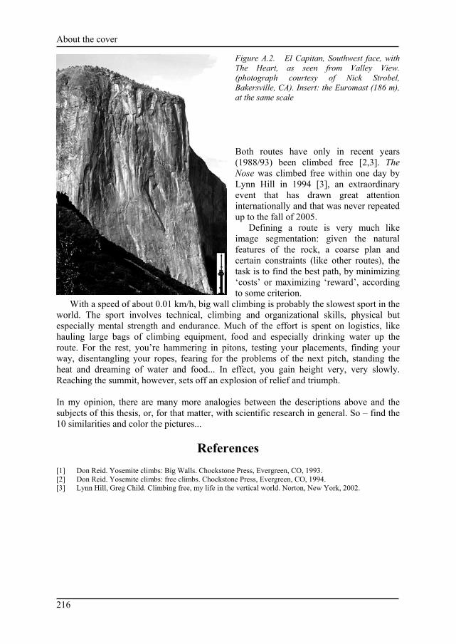
About the cover

216

Figure A.2. El Capitan, Southwest face, with The Heart, as seen from Valley View. (photograph courtesy of Nick Strobel, Bakersville, CA). Insert: the Euromast (186 m), at the same scale

Both routes have only in recent years (1988/93) been climbed free [2,3]. The Nose was climbed free within one day by Lynn Hill in 1994 [3], an extraordinary event that has drawn great attention internationally and that was never repeated up to the fall of 2005.

Defining a route is very much like image segmentation: given the natural features of the rock, a coarse plan and certain constraints (like other routes), the task is to find the best path, by minimizing ‘costs’ or maximizing ‘reward’, according to some criterion.

With a speed of about 0.01 km/h, big wall climbing is probably the slowest sport in the world. The sport involves technical, climbing and organizational skills, physical but especially mental strength and endurance. Much of the effort is spent on logistics, like hauling large bags of climbing equipment, food and especially drinking water up the route. For the rest, you’re hammering in pitons, testing your placements, finding your way, disentangling your ropes, fearing for the problems of the next pitch, standing the heat and dreaming of water and food... In effect, you gain height very, very slowly. Reaching the summit, however, sets off an explosion of relief and triumph. In my opinion, there are many more analogies between the descriptions above and the subjects of this thesis, or, for that matter, with scientific research in general. So – find the 10 similarities and color the pictures...

References [1] Don Reid. Yosemite climbs: Big Walls. Chockstone Press, Evergreen, CO, 1993. [2] Don Reid. Yosemite climbs: free climbs. Chockstone Press, Evergreen, CO, 1994. [3] Lynn Hill, Greg Child. Climbing free, my life in the vertical world. Norton, New York, 2002.

217

Full color supplement

Figure 1.3

Figure 1.4

Figure 3.7 Figure 5.4

Full color supplement

218

(a) (b)

(c) Figure 5.5

Figure 5.8 Figure 6.1

Full color supplement

219

Figure 7.5

Figure 7.12

Figure 7.19

Full color supplement

220

Figure 7.13

Figure 7.14 (Figure 7.19: see previous page)

221

Publications

This section lists publications by the author of this thesis in chronological order, divided in two parts: full papers (journal papers, conference papers, book chapters), and abstracts.

Full papers (journal and conference papers, book chapters) 1. Leliveld WH, Bosch JG, Mathijssen RWM, Ossevoort HJM. The monoselector. An electronic aid for

environmental remote control of electrical appliances for paralyzed persons. Medical Progress through Technology 1988;13:165-170.

2. Bosch JG, Reiber JHC, van Burken G, Gerbrands JJ, Gussenhoven EJ, Bom N, Roelandt JRTC. Automated endocardial contour detection in short-axis 2-D echocardiograms: methodology and assessment of variability. In: Ripley KL, ed. Computers in Cardiology; 1988; Washington DC: IEEE Computer Society Press; p. 137-140.

3. Bosch HG, Reiber JHC, van Burken G, Gerbrands JJ, Roelandt JRTC. Automated contour detection on short-axis transesophageal echocardiograms. In: Erbel R, Khanderia BK, Brennecke R, Meyer J, Seward JB, Tajik AJ, editors. Transesophageal Echocardiography - A new window to the heart. Berlin: Springer; 1988. p. 253-259.

4. Gussenhoven EJ, Essed CE, Lancée CT, Mastik F, Frietman P, van Egmond FC, Reiber JHC, Bosch JG, van Urk H, Roelandt JRTC, Bom N. Arterial wall characteristics determined by intravascular ultrasound imaging: an in vitro study. J Am Coll Cardiol 1989;14(4):947-952.

5. Bom N, ten Hoff H, Lancée CT, Gussenhoven WJ, Bosch JG. Early and recent intraluminal ultrasound devices. Int J Cardiac Imaging 1989;4:79-88.

6. Bom N, Bosch JG, Reiber JHC, Gussenhoven EJ, Slager CJ, Brower RW. Current intra-arterial ultrasound imaging systems and automatic contour detection. In: Reiber JHC, Serruys PW, editors. Quantitative Coronary Arteriography. Dordrecht: Kluwer; 1990. p. 199-210.

7. Li W, Gussenhoven WJ, Bosch JG, Mastik F, Reiber JHC, Bom N. A computer-aided analysis system for the quantitative assessment of intravascular ultrasound images. In: Ripley KL, ed. Computers in Cardiology; 1990; Chicago: IEEE Computer Society Press; p. 333-336.

8. Bosch JG, Reiber JHC, van Burken G, Gerbrands JJ, Kostov A, van de Goor AJ, van Daele MERM, Roelandt JRTC. Developments towards real-time frame-to-frame automatic contour detection in echocardiograms. In: Ripley KL, ed. Computers in Cardiology; 1990; Chicago: IEEE Computer Society Press; p. 435-438.

9. Bom N, Reiber JHC, Lancée CT, Bosch JG, Roelandt JRTC, Lachmann B. Technik für intraluminales Monitoring von Herz und Blutgefäßen mit Ultraschall. In: Versprille A, editor. Monitoring. (Anaesthesiologie und Intensivmedizin; 224). Berlin: Springer; 1992. p. 45-54.

10. Li W, Bosch JG, Zhong Y, Gussenhoven WJ, Rijsterborgh H, Reiber JHC, Bom N. Semiautomatic frame-to-frame tracking of the luminal border from intravascular ultrasound. In: Murray A, ed. Computers in Cardiology; 1991; Venice, Italy: IEEE Computer Society Press; p. 353-356.

11. Bosch JG, van Burken G, Reiber JHC. Automated frame-to-frame contour detection in echocardiograms using motion estimation. In: Murray A, ed. Computers in Cardiology; 1992; Durham, NC: IEEE Computer Society Press; p. 351-354.

12. Bot H,Delemarre BJ,Bosch JG,Visser CA.Automation in echocardiography.Neth J Cardiol1993;3:161-167 13. Li W, Bosch JG, Zhong Y, The SHK, Gussenhoven WJ, Mastik F, van Egmond FC, Rijsterborgh H,

Reiber JHC, Bom N. Image segmentation and 3D reconstruction of intravascular ultrasound images. In: Wei Y, Gu B, editors. Acoustical Imaging vol. 20. New York: Plenum Press; 1992. p. 489-496.

14. Reiber JHC, Koning G, van der Zwet PMJ, Bosch HG, van Meurs B, Schalij MJ, Buis B, Zijlstra F. Assessment of myocardial flow reserve with the DCI. MedicaMundi 1993;38(2):81-88.

15. Reiber JHC, van der Zwet PMJ, von Land CD, Koning G, Bosch JG, van der Geest RJ. New developments in cardiovascular image processing applications. In: Mortier E, Poelaert J, editors. Update in cardiac surgery, anesthesia and intensive care. Ghent; 1993. p. 113-114.

Publications

222

16. Sosef MN, Bosch JG, van Oostayen JA, Visser T, Reiber JHC, Rosendaal FR. Relation of plasma coagulation factor VII and fibrinogen to carotid artery intima-media thickness. Thromb Haemost 1994;72(2):250-254.

17. Reiber JHC, van der Zwet PMJ, Koning G, von Land CD, Bosch JG, Maurincomme E, van der Geest RJ, Gerbrands JJ. Perspectieven in beeldvorming en beeldverwerking. In: Verheugt FWA, Bos KW, editors. De toekomst van de cardiologie: Nederlandse Hartstichting; 1994. p. 63-91.

18. Bosch JG, Reiber JHC, van Burken G, Savalle LH, Maurincomme E, Helbing WA. Automated contour detection and acoustic quantification. Eur Heart J 1995;16(Suppl J):35-41.

19. Bosch JG, van Burken G, Schukking SS, Wolff R, van de Goor AJ, Reiber JHC. Real-time frame-to-frame automatic contour detection on echocardiograms. In: Murray A, ed. Computers in Cardiology; 1994; Bethesda, MD: IEEE Computer Society Press; p. 29-32.

20. Bosch JG, Savalle LH, van Burken G, Reiber JHC. Evaluation of a semiautomatic contour detection approach in sequences of short-axis two-dimensional echocardiographic images. J Am Soc Echocardiogr 1995;8(6):810-821.

21. Helbing WA, Bosch HG, Maliepaard C, Rebergen SA, van der Geest RJ, Hansen B, Ottenkamp J, Reiber JHC, de Roos A. Comparison of echocardiographic methods with magnetic resonance imaging for assessment of right ventricular function in children. Am J Cardiol 1995;76(8):589-594.

22. Helbing WA, Bosch HG, Maliepaard C, Zwinderman KH, Rebergen SA, Ottenkamp J, de Roos A, Reiber JHC. On-line automated border detection for echocardiographic quantification of right ventricular size and function in children. Pediatr Cardiol 1997;18(4):261-269.

23. Li W, The SHK, Wilson RA, Bosch JG, Gussenhoven EJ, Di Mario C, Reiber JHC, Bom N, Verdouw PD, Roelandt JRTC. Semi-automatic frame-to-frame tracking of the luminal border from intravascular ultrasound: technical development and clinical applications. In: Li W, editor. Image and signal processing in intravascular ultrasound (PhD Thesis). Rotterdam: Erasmus University Rotterdam; 1997. p. 33-45.

24. Li W, von Birgelen C, Hartlooper A, van der Lugt A, van Egmond FC, Di Mario C, Boersma E, van der Putten N, Bosch JG, Gussenhoven EJ, Reiber JHC, Bom N, Roelandt JRTC. Three-dimensional reconstruction and volumetric quantification of intravascular ultrasound. In: Li W, editor. Image and signal processing in intravascular ultrasound (PhD Thesis). Rotterdam: Erasmus University Rotterdam; 1997. p. 47-67.

25. Reiber JHC, Goedhart B, Bosch HG, van der Geest RJ, Dijkstra J, Koning G, Ramze Rezaee M, Lelieveldt BPF, de Roos A, van der Wall EE, Bruschke AVG. Quantitative cardiovascular image analysis: current status and what are realistic expectations for the future? In: van der Wall EE, Manger Cats V, Baan J, editors. Vascular Medicine - From Endothelium to Myocardium. Dordrecht: Kluwer; 1997. p. 103-131.

26. Bosch HG, van Burken G, Nijland F, Reiber JHC. Overview of automated quantitation techniques in 2D echocardiography. In: Reiber JHC, van der Wall EE, editors. What's new in cardiovascular imaging. (Developments in cardiovascular medicine). Dordrecht, the Netherlands: Kluwer; 1998. p. 363-376.

27. Šrámek A, Bosch JG, Reiber JHC, van Oostayen JA, Rosendaal FR. Ultrasound assessment of atherosclerotic vessel wall changes - Reproducibility of intima-media thickness measurements in carotid and femoral arteries. Invest Radiol 2000;35(12):699-706.

28. Lelieveldt BPF, van der Geest RJ, Ramze Rezaee M, Bosch JG, Reiber JHC. Anatomical model matching with fuzzy implicit surfaces for segmentation of thoracic volume scans. IEEE Trans Med Imaging 1999;18(3):218-230.

29. van Assen HC, Vrooman HA, Egmont-Petersen M, Bosch HG, Koning G, Van der Linden EL, Goedhart B, Reiber JHC. Automated calibration in vascular X-ray images using the accurate localization of catheter marker bands. Invest Radiol 2000;35(4):219-226.

30. Mitchell SC, Lelieveldt BPF, van der Geest RJ, Bosch HG, Reiber JHC, Sonka M. Multistage hybrid active appearance model matching: Segmentation of left and right ventricles in cardiac MR images. IEEE Trans Med Imaging 2001;20(5):415-423.

31. Lelieveldt BPF, Mitchell SC, Bosch JG, van der Geest RJ, Sonka M, Reiber JHC. Time-continuous segmentation of cardiac image sequences using Active Appearance Motion Models. In: Insana MF, Leahy RM, eds. Information Processing in Medical Imaging (IPMI), LNCS2082; 2001; Davis, CA: Springer; p. 446-452.

32. Bosch JG, Reiber JHC. Two-dimensional echocardiographic digital image processing and approaches to endocardial edge detection. In: Otto CM, editor. The practice of clinical echocardiography. Second ed. Orlando, FL: W.B. Saunders; 2002. p. 141-158.

33. Bosch HG, Mitchell SC, Lelieveldt BPF, Nijland F, Kamp O, Sonka M, Reiber JHC. Active Appearance Motion Models for endocardial contour detection in time sequences of echocardiograms. In: Sonka M, Hanson KM, eds. SPIE Medical Imaging: Image Processing, vol 4322; 2001; San Diego: SPIE; p. 257-268.

Publications

223

34. Mitchell SC, Lelieveldt BPF, van der Geest RJ, Bosch HG, Reiber JHC, Sonka M. Time continuous seg-mentation of cardiac MR image sequences using active appearance motion models. In: Sonka M, Hanson KM, eds. SPIE Medical Imaging: Image Processing, vol 4322; 2001; San Diego: SPIE; p. 249-256.

35. Bosch HG, Mitchell SC, Lelieveldt BPF, Nijland F, Kamp O, Sonka M, Reiber JHC. Active Appearance-Motion Models for fully automated endocardial contour detection in time sequences of echocardiograms. In: Lemke HU, Vannier MW, Inamura K, Farman G, Doi K, eds. Computer Assisted Radiology and Surgery (CARS), ICS1230; 2001; Berlin: Elsevier; p. 896-901.

36. Lelieveldt BPF, Mitchell SC, van der Geest RJ, Bosch HG, Sonka M, Reiber JHC. Time continuous segmentation of cardiac MR images using Active Appearance Motion Models. In: Lemke HU, Vannier MW, Inamura K, Farman G, Doi K, eds. Computer Assisted Radiology and Surgery (CARS), ICS1230; 2001; Berlin: Elsevier; p. 917-921.

37. Sonka M, Lelieveldt BPF, Mitchell SC, Bosch JG, van der Geest RJ, Reiber JHC. Active appearance motion model segmentation. In: 2nd int workshop Digital and Computational Video; 2001; Tampa, FL: IEEE Computer Society Press; p. 64-68.

38. Bosch JG, Mitchell SC, Lelieveldt BPF, Nijland F, Kamp O, Sonka M, Reiber JHC. Fully automated endocardial contour detection in time sequences of echocardiograms by Active Appearance-Motion Models. In: Murray A, ed. Computers in Cardiology 28; 2001; Rotterdam: IEEE Computer Society Press; p. 93-96.

39. Bovenkamp EGP, Dijkstra J, Bosch JG, Reiber JHC. Collaborative multi-agent IVUS image segmentation. Medical Image Computing and Computer-Assisted Intervention - MICCAI 2001, LNCS2208; 2001: 1185-1186.

40. Bovenkamp EGP, Dijkstra J, Bosch JG, Reiber JHC. Multi-agent IVUS image segmentation. In: Kröse B, de Rijke M, Schreiber G, van Someren M, eds. 13th Belgium-Netherlands Conference on Artificial Intelligence (BNAIC); 2001; Amsterdam: Amsterdam University Press; p. 357-364.

41. Bosch JG, Mitchell SC, Lelieveldt BPF, Nijland F, Kamp O, Sonka M, Reiber JHC. Automatic segmentation of echocardiographic sequences by active appearance motion models. IEEE Trans Med Imaging 2002;21(11):1374-1383.

42. Mitchell SC, Bosch JG, Lelieveldt BPF, van der Geest RJ, Reiber JHC, Sonka M. 3-D active appearance models: segmentation of cardiac MR and ultrasound images. IEEE Trans Med Imaging 2002;21(9):1167-1178.

43. Bosch JG, Mitchell SC, Lelieveldt BPF, Nijland F, Kamp O, Sonka M, Reiber JHC. Fully automated endocardial contour detection in time sequences of echocardiograms by three-dimensional Active Appearance Models. In: Sonka M, Fitzpatrick JM, eds. SPIE Medical Imaging: Image Processing, vol 4684; 2002; San Diego: SPIE; p. 452-462.

44. Mitchell SC, Lelieveldt BPF, Bosch JG, van der Geest RJ, Reiber JHC, Sonka M. Segmentation of cardiac MR volume data using 3D active appearance models. In: Sonka M, Fitzpatrick JM, eds. SPIE Medical Imaging: Image Processing, vol 4684; 2002; San Diego: SPIE; p. 433-443.

45. Lelieveldt BPF, Mitchell SC, Bosch JG, van der Geest RJ, Sonka M, Reiber JHC. 3D active appearance models: application to cardiac MR and ultrasound image segmentation. In: Lemke HU, Vannier MW, Inamura K, Farman G, Doi K, Reiber JHC, eds. Computer Assisted Radiology and Surgery (CARS); 2002; Paris: Springer; p. 897-901.

46. Nijland F, Kamp O, Verhorst PMJ, de Voogt WG, Bosch HG, Visser CA. Myocardial viability: impact on left ventricular dilatation after acute myocardial infarction. Heart 2002;87(1):17-22.

47. Cain P, Short L, Baglin T, Case C, Bosch HG, Marwick TH. Development of a fully quantitative approach to the interpretation of stress echocardiography using radial and longitudinal myocardial velocities. J Am Soc Echocardiogr 2002;15(8):759-767.

48. Bovenkamp EGP, Dijkstra J, Bosch JG, Reiber JHC. Multi-agent segmentation of IVUS images. Pattern Recognition 2004;37(4):647-663.

49. Bosch JG, Nijland F, Mitchell SC, Lelieveldt BPF, Kamp O, Sonka M, Reiber JHC. Automated classification of wall motion abnormalities by Principal Component Analysis of endocardial shape motion patterns in echocardiograms. In: Sonka M, Fitzpatrick JM, eds. SPIE Medical Imaging: Image Processing, vol 5032; 2003; San Diego: SPIE; p. 38-49.

50. Mitchell SC, Lelieveldt BPF, Bosch HG, Reiber JHC, Sonka M. Disease characterization of active appearance model coefficients. In: Sonka M, Fitzpatrick JM, eds. SPIE Medical Imaging: Image Processing, vol 5032; 2003; San Diego: SPIE; p. 949-957.

51. Bovenkamp EGP, Dijkstra J, Bosch JG, Reiber JHC. Multi-agent IVUS image interpretation. In: Sonka M, Fitzpatrick JM, eds. SPIE Medical Imaging: Image Processing, vol 5032; 2003; San Diego: SPIE; p. 619-630.

52. Sonka M, Bosch JG, Lelieveldt BPF, Mitchell SC, Reiber JHC. Computer-aided diagnosis via model-based shape analysis: cardiac MR and echo. In: Lemke HU, Vannier MW, Inamura K, Farman G, Doi K,

Publications

224

Reiber JHC, eds. Computer Assisted Radiology and Surgery (CARS), ICS1256; 2003; London: Esevier; p. 1013-1018.

53. Bovenkamp EGP, Dijkstra J, Bosch JG, Reiber JHC. Multi-agent segmentation of IVUS images. In: Heskes T, Lucas P, Vuurpijl L, Wiegerink W, eds. 15th Belgium-Netherlands Conference on Artificial Intelligence (BNAIC); 2003; Nijmegen; p. 395-396.

54. van Stralen M, Bosch JG, Voormolen MM, van Burken G, Krenning BJ, Lancée CT, de Jong N, Reiber JHC. A semi-automatic endocardial border detection method for the left ventricle in 4D ultrasound data sets. In: Lemke HU, Vannier MW, Inamura K, Farman G, Doi K, Reiber JHC, eds. Computer Assisted Radiology and Surgery (CARS), ICS1268; 2003; Chicago: Esevier; p. 1078-1083.

55. van Stralen M, Bosch JG, Voormolen MM, van Burken G, Krenning BJ, Lancée CT, de Jong N, Reiber JHC. A semi-automatic endocardial border detection method for 4D ultrasound data. Medical Image Computing and Computer-Assisted Intervention - MICCAI 2004, Pt 1, LNCS3216; 2004: 43-50.

56. Warda HM, Bax JJ, Bosch JG, Atsma DE, Jukema JW, van der Wall EE, van der Laarse A, Schalij MJ, Oemrawsingh PV. Effect of intracoronary aqueous oxygen on left ventricular remodeling after anterior wall ST-elevation acute myocardial infarction. Am J Cardiol 2005;96(1):22-24.

57. Bosch JG, Nijland F, Mitchell SC, Lelieveldt BPF, Kamp O, Reiber JHC, Sonka M. Computer-aided diagnosis via model-based shape analysis: Automated classification of wall motion abnormalities in echocardiograms. Acad Radiol 2005;12(3):358-367.

58. van Stralen M, Bosch JG, Voormolen MM, van Burken G, Krenning BJ, Lancée CT, de Jong N, Reiber JHC. Left ventricular volume estimation in cardiac 3D ultrasound: a semi-automatic border detection approach. Acad Radiol 2005;12:1241-1249.

59. Janssen JP, Koning G, de Koning PJ, Bosch JG, Tuinenburg JC, Reiber JHC. A new approach to contour detection in x-ray arteriograms: the wavecontour. Invest Radiol 2005;40(8):514-20.

60. van Stralen M, Bosch JG, Voormolen MM, van Burken G, Krenning BJ, van Geuns RJM, Angelie E, van der Geest RJ, Lancée CT, de Jong N, Reiber JHC. Semi-automatic border detection method for left ventricular volume estimation in 4D ultrasound data. In: Fitzpatrick JM, ed. SPIE Medical Imaging: Image Processing, vol 5747; 2005; San Diego: SPIE; p. 1457-1467.

61. Bovenkamp EGP, Dijkstra J, Bosch JG, Reiber JHC. User-agent cooperation in multi-agent IVUS image segmentation. IEEE Trans Med Imaging 2006:submitted.

62. van Stralen M, Bosch JG, Voormolen MM, van Burken G, Krenning BJ, van Geuns RJM, Angelié E, Lancée CT, de Jong N, Reiber JHC. Semi-automatic border detection method for left ventricular volume estimation in 4D ultrasound data. In: 11th ASCI conf; 2005; Heijen, NL; p. 200-207.

63. Bosch JG. Automatic analysis of echocardiographic studies - the final frontier? Int J Cardiovasc Imaging 2005;21:627-628.

64. Bosch JG, van Stralen M, Voormolen MM, Krenning BJ, Lancée CT, Reiber JHC, van der Steen AFW, de Jong N. Improved spatiotemporal voxel space interpolation for 3D echocardiography with irregular sampling and multibeat fusion. In: Proceedings 2005 IEEE International Ultrasonics Symposium, Rotterdam, p. 1232-1235.

65. van Stralen M, Voormolen MM, van Burken G, Krenning BJ, van Geuns RJM, Angelié E, van der Geest RJ, Lancée CT, de Jong N, van der Steen AFW, Reiber JHC, Bosch JG. A novel dynamic programming based semi-automatic endocardial border detection method for 4D cardiac ultrasound. In: Proceedings 2005 IEEE International Ultrasonics Symposium, Rotterdam, p. 1224-1227.

66. Bosch JG, van Stralen M, Voormolen MM, Krenning BJ, Lancée CT, Reiber JHC, van der Steen AFW, de Jong N. Novel spatiotemporal voxel interpolation with multibeat fusion for 3D echocardiography with irregular data distribution. In: Emelianov S, Walker WF, eds. SPIE Medical Imaging: Ultrasonic Imaging & Image Processing, vol 6147; 2006; San Diego: SPIE; paper 61470Q p.1-11.

67. Leung KYE, van Stralen M, Voormolen MM, van Burken G, Nemes A, ten Cate FJ, Geleijnse ML, de Jong N, Reiber JHC, Bosch JG. Registration of 2D cardiac images to real-time 3D ultrasound volumes for 3D stress echocardiography. In: Reinhardt JM, Pluim JP, eds. SPIE Medical Imaging: Image Processing, vol 6144; 2006; San Diego: SPIE; paper 614418 p. 1-12.

68. Nemes A, Geleijnse ML, Bosch JG, Soliman OII, Anwar AM, Krenning BJ, Vletter WB, ten Cate FJ. Current status of real-time three-dimensional stress echocardiography. Submitted March 2006.

Published abstracts 68. Bosch JG, Reiber JHC, van Burken G, Gerbrands JJ, Gussenhoven EJ, Roelandt JRTC. Quantitative

esophageal short-axis echocardiography with automatic endocardial contour detection. Eur Heart J 1988;9(Suppl 1):378.

Publications

225

69. van Daele M, Bosch HG, Reiber H, Sutherland GR, Roelandt JRTC. Can changes in cardiac output during surgery be monitored by transesophageal echo and computer-assisted analysis? Int J Cardiac Imaging 1989;4(1):70.

70. Bosch JG, Reiber JHC, van Burken G, Gerbrands JJ, Gussenhoven WJ, Bom N, Roelandt JRTC. Automated contour detection on short-axis echocardiograms. In: 8th int symp Echocardiology; 1989; Rotterdam; p. 77.

71. van Daele M, Bosch HG, Reiber H, Sutherland GR, Roelandt JRTC. Monitoring changes in cardiac output by transesophageal echo and computer-supported analysis: is it feasible? Eur Heart J 1989;10(Suppl):179.

72. Bosch JG, Reiber JHC, van Burken G, Gerbrands JJ, van Daele MERM, Roelandt JRTC. Automated endocardial contour detection on short-axis TEE echocardiograms. In: Abstract book Symposium Slokdarm Echocardiografie AMC. Amsterdam: Academisch Medisch Centrum; 1990. p. 18.

73. van der Zwet PMJ, Reiber JHC, Koning G, Bosch HG, van Benthem AC, Padmos I, Buis B, van Meurs B. Myocard flow reserve on DCI. In: Abstract book COMETT Training Course Quality Assurance in Digital Angiography; 1991; Kiel; p. 20b.

74. van der Zwet PMJ, Bosch JG, Willems J, Koning G, van Benthem AC, Begeman C, Buis B, van Meurs B, Reiber JHC. On-line myocard flow reserve; basic principles. In: Abstract book 4th International Symposium on Coronary Arteriography; 1991; p. 190.

75. Bosch JG, von Land CD, Reiber JHC. Storage media for cardiac image analysis workstations. In: Workshop Integrating Cardiology Information Systems (INCIS); 1992; Mainz: ESC working group Computers in Cardiology; p. B1.

76. Bosch JG, van Burken G, Reiber JHC. Automatic frame-to-frame contour detection in echocardiograms using motion estimation. In: Abstract book 10th Symp on Echocardiology; 1993; Rotterdam; p. 165.

77. Reiber JHC, Bosch JG, van Burken G. Automated Contour Detection - motivation and present state of the art. In: Abstract book 10th Symp on Echocardiology. Erasmus University Rotterdam; 1993. p. 115.

78. Helbing WA, Maliepaard C, Rebergen SA, Bosch HG, Ottenkamp J, de Roos A, Reiber JHC. Right ventricular function: assessment with echocardiography and correlation with magnetic resonance imaging. Cardiology in the Young 1994;4:22.

79. Bosch JG, van Burken G, Savalle LH, Reiber JHC. Automated endocardial border detection in sequences of echocardiograms. J Am Soc Echocardiogr 1994;3(part 2 supplement):S39.

80. Helbing WA, Maliepaard C, Bosch HG, Ottenkamp J, Reiber JHC. Echocardiographic quantification of right ventricular areas in children by automatic border detection. Eur Heart J 1994;15(abstract suppl):501.

81. Picard MH, Bosch HG, Morrissey RL, Reiber JHC. Automated echocardiographic ventricular volume quantitation - validation of a new border detection method. Circulation 1994;90(4 Suppl):I-608.

82. Bosch JG, Reiber JHC, van Burken G, Savalle LH. Automated endocardial border detection in sequences of echocardiograms. In: 61 Jahrestagung der Deutschen Gesellschaft für Kardiologie - Herz- und Kreislaufforschung; 1995; Mannheim; p. Abstract 184.

83. Reiber JHC, Bosch JG, van Burken G, Savalle LH. Automatic contour detection in two-dimensional echocardiographic sequences. In: Abstract book 11th Symp on Echocardiology; 1995; Rotterdam; p. 176.

84. Helbing WA, Maliepaard C, Bosch HG, de Roos A, Ottenkamp J, Reiber JHC. Automated border detection in echocardiographic quantification of right ventricular function in children: comparison with magnetic resonance imaging. Circulation 1995;92(8 Suppl I):I-442.

85. Nijland F, Kamp O, Verhorst PMJ, de Voogt WG, Bosch HG, Visser CA. Myocardial viability: impact on left ventricular dilatation after acute myocardial infarction. Cardiologie 1997;4:483.

86. Nijland F, Kamp O, Verhorst PMJ, de Voogt WG, Bosch HG, Visser CA. Impact of myocardial viability on left ventricular dilatation following acute myocardial infarction. J Am Coll Cardiol 1998;31(2 suppl A):408A.

87. Fry SJ, Hunziker PR, Bosch HG, Reiber JHC, Picard MH. Automated echocardiographic confirmation of regional wall motion abnormalities: quantitation of continuous LV volume. J Am Coll Cardiol 1998;31(2 suppl. A):56A.

88. Schöb L, Hunziker PR, Bosch HG, Füllhaas U, Hess N, Pfisterer M, Buser P. Automatic border detection zur Quantifizierung der Wandmotilität in der Stressechokardiographie. Kardiovaskuläre Medizin 1999; 2(Suppl 1):19S.

89. Hunziker PR, Schöb L, Bosch HG, Hess N, Kaiser C, Pfisterer M, Buser P. Quantitative dobutamine stress echocardiography: new insights with automatic border detection. J Am Soc Echocardiogr 1999;12(5):386.

90. Hunziker PR, Schöb L, Lefkovits M, Füllhaas U, Yoon SI, Bosch HG, Cron T, Pfisterer M, Buser P. Automatic border detection in dobutamine stress echo: how do normal and ischaemic segments behave objectively and quantitatively? Eur Heart J 1999;20(abstract suppl):618.

91. Bosch JG, Nijland F, van Burken G, Reiber JHC. Feasibility of model-based automated border detection for quantification of stress echocardiography. In: Abstract book 13th Symp on Echocardiology; 1999; Rotterdam; p. 70.

Publications

226

92. Hunziker PR, Yuan D, Schöb L, Bosch HG, Pfisterer M, Buser P. Objective and quantitative stress echo analysis to diagnose coronary disease using model-based image processing. J Am Coll Cardiol 2000;35(2 suppl A):431A.

93. Bosch JG, Mitchell SC, Lelieveldt BPF, Sonka M, Nijland F, van Burken G, Reiber JHC. Feasibility of fully automated border detection on stress echocardiograms by Active Appearance Models. Eur Heart J 2000;21(abstract suppl):11.

94. Bosch JG, Mitchell SC, Lelieveldt BPF, Sonka M, Nijland F, Reiber JHC. Model-based automated border detection for quantitative stress echocardiography. Eur Heart J 2000;21(abstract suppl):37.

95. Lelieveldt BPF, van der Geest RJ, Mitchell SC, Bosch JG, Sonka M, Reiber JHC. Automated model-based segmentation of the right and left ventricular contours. Eur Heart J 2000;21(abstract suppl):582.

96. Bosch HG, Mitchell SC, Lelieveldt BPF, Sonka M, Nijland F, Reiber JHC. Feasibility of fully automated border detection on stress echocardiograms by active appearance models. Circulation 2000;102(18 Suppl II):633.

97. Bosch JG, Mitchell SC, Lelieveldt BPF, Sonka M, Nijland F, Kamp O, Reiber JHC. Fully automated border detection for stress echo by Active Appearance Models. Eur J Echocardiography 2000;1(suppl. 2):S34.

98. Lelieveldt BPF, van der Geest RJ, Mitchell SC, Bosch JG, Sonka M, Reiber JHC. Fully automated, time-continuous contour delineation of the endo- and epicardium in short-axis cardiac MR image sequences. Proc Int Soc Mag Reson Med 2001;9:600.

99. Lelieveldt BPF, Mitchell SC, Bosch JG, Sonka M, Reiber JHC, van der Geest RJ. Time-continuous automated contour detection of the endo- and epicardium in short-axis cardiac MR image sequences. Eur Heart J 2001;22(abstract suppl ESC Stokholm):352.

100. Bosch JG, Mitchell SC, Lelieveldt BPF, Nijland F, Kamp O, Sonka M, Reiber JHC. Fully automated endocardial border detection in sequences of echocardiograms by active appearance-motion models. Circulation 2001;104(17 suppl II):652.

101. Lelieveldt BPF, Mitchell SC, Bosch JG, van der Geest RJ, Sonka M, Reiber JHC. Automatic detection of endo- and epicardial contours in short-axis cardiac MR data using 3D active appearance models. J Cardiovasc Magn Res 2002;4(1):106-107.

102. Bosch JG, Nijland F, Kamp O, van Burken G, Sonka M, Reiber JHC. Automated classification of wall motion abnormalities by automated border detection and analysis of left ventricular endocardial motion patterns. J Am Soc Echocardiogr 2003;16(5):507.

103. Bosch JG, Nijland F, Kamp O, van Burken G, Sonka M, Reiber JHC. Automated classification of wall motion abnormalities by analysis of left-ventricular endocardial motion patterns. Eur Heart J 2003;24(abstract suppl):203.

104. Bosch JG, Nijland F, Mitchell SC, Lelieveldt BPF, Kamp O, Sonka M, Reiber JHC. Automated classification of wall motion abnormalities by analysis of left ventricular endocardial motion patterns. In: Abstract book Ned Ver v Cardiologie Scientific Meeting; 2003; Amsterdam; p. 125.

105. Bosch JG, Nijland F, Mitchell SC, Lelieveldt BPF, Kamp O, Sonka M, Reiber JHC. Automated classification of wall motion abnormalities by analysis of left ventricular endocardial contour motion patterns. Eur J Echocardiography 2003;4(suppl 1):S95.

106. van Stralen M, Bosch JG, Voormolen MM, van Burken G, Krenning BJ, van Geuns RJM, Lancée CT, de Jong N, Reiber JHC. Semi-automatic left ventricular endocardial border detection method for 4D ultrasound data. Eur J Echocardiography 2004;5(suppl 1):S57.

107. Warda HM, Bosch JG, Atsma DE, Jukema JW, van der Wall EE, Schalij MJ, Oemrawsingh PV. Intracoronary hyperbaric oxygen administered during primary percutaneous coronary intervention prevents one month left ventricular remodeling. Circulation 2004;110(17 suppl S):698.

108. Warda HM, Bosch JG, Bax JJ, Atsma DE, Jukema JW, van der Wall EE, Schalij MJ, Oemrawsingh PV. Intracoronary hyperbaric oxygen administered during primary percutaneous coronary intervention prevents 1-month left ventricular remodeling. Am J Cardiol 2004;94(suppl 6A):89E.

109. Warda HM, Oemrawsingh PV, Atsma DE, Bosch JG, Lindsay BS, van der Wall EE, Schalij MJ. Perfusion recovery after myocardial infarction diagnostic (PYRAMID) score; first angiographic predictor of future left ventricular remodeling after acute myocardial infarction. Am J Cardiol 2004;94(suppl 6A):15E.

110. Warda HM, Bosch JG, Bax JJ, Atsma DE, Jukema JW, van der Wall EE, Schalij MJ, Oemrawsingh PV. Intracoronary hyperbaric oxygen administered during primary percutaneous coronary intervention prevents one month left ventricular remodeling. J Am Coll Cardiol 2005;45(3 suppl 1):242A.

111. van Stralen M, Voormolen MM, Angelié E, Krenning BJ, van Geuns RJM, de Jong N, Reiber JHC, Bosch JG. Evaluation of automated full cycle left ventricular volume estimation for real-time 3D echo against MRI. Eur J Echocardiography 2005;6(suppl 1):S131.

227

Curriculum Vitae

Johannes Gijsbertus Bosch was born in Berlicum, Noord-Brabant, the Netherlands on July 1st, 1960. He received his secondary education at Gymnasium Bernrode in Heeswijk-Dinther, from which he obtained the diploma (Gymnasium-β) in June, 1978. In August 1985 he received the Master of Science degree (Ir.) in Electrical Engineering at Eindhoven University of Technology, Eindhoven, the Netherlands. His Master’s thesis was completed at the Division of Medical Electronics and concerned a speech recognition device for severely handicapped persons. As an alternative to military service, he performed 18 months of civil service at the Division of Medical Electronics, where he developed electronic aids for disabled persons, and supervised students.

In February 1987 he joined the Laboratory for Clinical and Experimental Image Processing (Laboratorium voor Klinische en Experimentele Beeldverwerking, LKEB) at the Thoraxcenter of the Erasmus University Rotterdam, and started his research on the automated analysis of echocardiographic images, under supervision of Dr. Ir. J.H.C. Reiber. When the LKEB was transferred to the Department of Radiology of the Leiden University Medical Center in 1990, he moved to Leiden as well. From 1995, he was the head of the section Echocardiography of the LKEB and Assistant Professor and continued the research on this subject, which has resulted in this thesis.

Since March 2005, he is employed as Assistant Professor and staff member at the department of Biomedical Engineering of the Thoraxcenter, Erasmus MC, Rotterdam, specialized in 2D and 3D echocardiographic image analysis.

He and his partner Simone Schellekens are proudly raising their two sons: Tom (2000) and Bram (2002).