End-to-End Defect Detection in Automated Fiber Placement ...
8
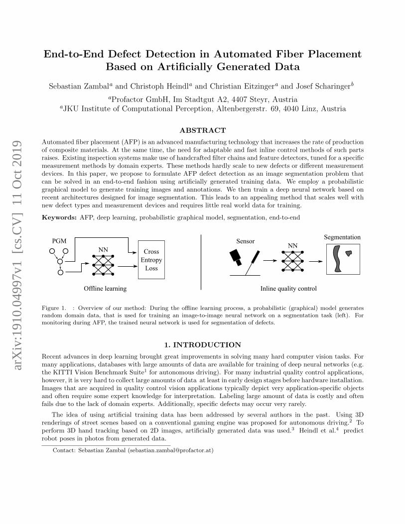
End-to-End Defect Detection in Automated Fiber Placement Based on Artificially Generated Data Sebastian Zambal a and Christoph Heindl a and Christian Eitzinger a and Josef Scharinger b a Profactor GmbH, Im Stadtgut A2, 4407 Steyr, Austria a JKU Institute of Computational Perception, Altenbergerstr. 69, 4040 Linz, Austria ABSTRACT Automated fiber placement (AFP) is an advanced manufacturing technology that increases the rate of production of composite materials. At the same time, the need for adaptable and fast inline control methods of such parts raises. Existing inspection systems make use of handcrafted filter chains and feature detectors, tuned for a specific measurement methods by domain experts. These methods hardly scale to new defects or different measurement devices. In this paper, we propose to formulate AFP defect detection as an image segmentation problem that can be solved in an end-to-end fashion using artificially generated training data. We employ a probabilistic graphical model to generate training images and annotations. We then train a deep neural network based on recent architectures designed for image segmentation. This leads to an appealing method that scales well with new defect types and measurement devices and requires little real world data for training. Keywords: AFP, deep learning, probabilistic graphical model, segmentation, end-to-end Offline learning Inline quality control Sensor NN Segmentation PGM NN Cross Entropy Loss Figure 1. : Overview of our method: During the offline learning process, a probabilistic (graphical) model generates random domain data, that is used for training an image-to-image neural network on a segmentation task (left). For monitoring during AFP, the trained neural network is used for segmentation of defects. 1. INTRODUCTION Recent advances in deep learning brought great improvements in solving many hard computer vision tasks. For many applications, databases with large amounts of data are available for training of deep neural networks (e.g. the KITTI Vision Benchmark Suite 1 for autonomous driving). For many industrial quality control applications, however, it is very hard to collect large amounts of data at least in early design stages before hardware installation. Images that are acquired in quality control vision applications typically depict very application-specific objects and often require some expert knowledge for interpretation. Labeling large amount of data is costly and often fails due to the lack of domain experts. Additionally, specific defects may occur very rarely. The idea of using artificial training data has been addressed by several authors in the past. Using 3D renderings of street scenes based on a conventional gaming engine was proposed for autonomous driving. 2 To perform 3D hand tracking based on 2D images, artificially generated data was used. 3 Heindl et al. 4 predict robot poses in photos from generated data. Contact: Sebastian Zambal ([email protected]) arXiv:1910.04997v1 [cs.CV] 11 Oct 2019
-
Upload
khangminh22 -
Category
Documents
-
view
3 -
download
0
Transcript of End-to-End Defect Detection in Automated Fiber Placement ...
End-to-End Defect Detection in Automated Fiber PlacementBased on Artificially Generated Data
Sebastian Zambala and Christoph Heindla and Christian Eitzingera and Josef Scharingerb
aProfactor GmbH, Im Stadtgut A2, 4407 Steyr, AustriaaJKU Institute of Computational Perception, Altenbergerstr. 69, 4040 Linz, Austria
ABSTRACT
Automated fiber placement (AFP) is an advanced manufacturing technology that increases the rate of productionof composite materials. At the same time, the need for adaptable and fast inline control methods of such partsraises. Existing inspection systems make use of handcrafted filter chains and feature detectors, tuned for a specificmeasurement methods by domain experts. These methods hardly scale to new defects or different measurementdevices. In this paper, we propose to formulate AFP defect detection as an image segmentation problem thatcan be solved in an end-to-end fashion using artificially generated training data. We employ a probabilisticgraphical model to generate training images and annotations. We then train a deep neural network based onrecent architectures designed for image segmentation. This leads to an appealing method that scales well withnew defect types and measurement devices and requires little real world data for training.
Keywords: AFP, deep learning, probabilistic graphical model, segmentation, end-to-end
Offline learning Inline quality control
SensorNN
SegmentationPGM
NN CrossEntropy
Loss
Figure 1. : Overview of our method: During the offline learning process, a probabilistic (graphical) model generatesrandom domain data, that is used for training an image-to-image neural network on a segmentation task (left). Formonitoring during AFP, the trained neural network is used for segmentation of defects.
1. INTRODUCTION
Recent advances in deep learning brought great improvements in solving many hard computer vision tasks. Formany applications, databases with large amounts of data are available for training of deep neural networks (e.g.the KITTI Vision Benchmark Suite1 for autonomous driving). For many industrial quality control applications,however, it is very hard to collect large amounts of data at least in early design stages before hardware installation.Images that are acquired in quality control vision applications typically depict very application-specific objectsand often require some expert knowledge for interpretation. Labeling large amount of data is costly and oftenfails due to the lack of domain experts. Additionally, specific defects may occur very rarely.
The idea of using artificial training data has been addressed by several authors in the past. Using 3Drenderings of street scenes based on a conventional gaming engine was proposed for autonomous driving.2 Toperform 3D hand tracking based on 2D images, artificially generated data was used.3 Heindl et al.4 predictrobot poses in photos from generated data.
Contact: Sebastian Zambal ([email protected])
arX
iv:1
910.
0499
7v1
[cs
.CV
] 1
1 O
ct 2
019
In this paper, we propose a novel structured approach for the use of artificial data to enable the applicationof machine learning methods for a specific quality control vision application: Monitoring of automated fiberplacement (AFP) processes. The vision system involved is a laser triangulation sensor that is mounted on thelay-up machinery. This sensor delivers depth information immediately after placement of carbon fiber tows. Weemploy a probabilistic graphical model to describe the creation of depth maps. Expert knowledge and processparameters can easily be included into the model. Depth maps sampled from the model are used to train adeep neural network to perform the actual task of image segmentation. A real data example is used to assesssegmentation performance of the deep neural network that was exclusively trained on artificial data.
2. RELATED WORK
Data generation The lack of annotated datasets for supervised machine learning has begun to impede theadvance of successful usage of such methods in industrial applications. To cope with this problem, a varietyof methods have been proposed. Active learning methods5,6 better involve domain experts by presenting onlythose data samples of high value to the current training progress. Semi-supervised learning7 transfers annotationsfrom small labeled datasets to larger unlabeled ones by making task-specific smoothness assumptions. Weaklysupervised learning8 attempts to infer precise labels from noisier, more global annotations, which are often easierto obtain. Transfer learning9 limits the amount of required training data by adapting pre-trained models tospecific tasks.
In contrast, methods that make use of artificial data generation utilize a simulation engine that generatesdata along with ground truth labels. Such methods are gaining popularity,2,4, 10 due to the availability of generalpurpose simulation engines. Like in this work, the simulator is driven by samples from a probabilistic modelthat has to be designed specific for the task at hands.
Segmentation Image segmentation is the task of partitioning an image into regions of common character-istics. Early works include image thresholding11 and clustering.12 With the raise of Convolutional Neural Nets(CNNs), image segmentation13,14 is understood as image-to-image conversion. U-Nets,15 which this work buildsupon, consist of contracting and expanding data paths. This assures that global context and local details areboth exploited to calculate the final segmentation result.
In contrast to the present work, quality inspection of automated fiber placement (AFP) is rarely formalizedas segmentation problem that is learned end-to-end. Frequently, pipelines consisting of handcrafted filters andfeature detectors are proposed, which are tuned for specific measurement devices. Cemenska et al.16 proposesautomatic detection of ply boundaries and tow ends based on laser profilometers. Juarez et al.17 studies theusage of thermographic cameras for gap detection based on heat diffusion. Similarly, Denkena et al.18 usethermographic inspection to detect overlaps, gaps, twisted tows and bridges based on thresholding.
3. QUALITY CONTROL FOR AUTOMATED FIBER PLACEMENT
For production of carbon fiber reinforced plastics (CFRP) parts, typically layers of carbon fiber material areplaced one layer after the other on some tooling. In automated fiber placement (AFP) this is done by largemachines that are able to automatically lay-up tows (stripes of carbon fiber material). Typically, these machinesare able to lay-up 8, 16, or even 32 tows in parallel next to each other. In order to assure mechanical stabilityof the final parts, it must be verified that carbon fibers are placed in the right way. There is a set of possibledefects that relate either to incorrect placement of tows or foreign objects.
While our method generalizes to any measurement method, we propose the use of a laser triangulation sensorto perform inline quality control. The type of data acquired by such a system is a sequence of laser line profiles.Our system accumulates multiple such profiles into a depth map where individual pixels describe depth. We arenot so much interested in absolute depth values. Rather, we focus on small depth variations that reveal differentdefects on the surface. The specific surface defects that we address here are:
• Gaps: Irregular larger spacings between neighboring tows.
• Overlaps: Irregular overlaps of tows that should actually be placed next to each other.
SD
G
X
YZ
F
w h t
R
Global parameters
Tow geometry
Plain depth mapand labels
Further randomization
50 0 50 100 150 200 250 300 350
50
0
50
100
150
200
250
L
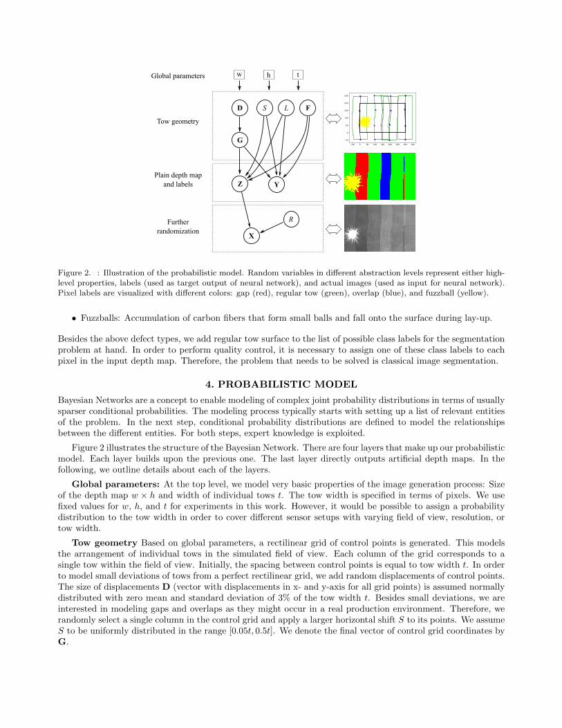
Figure 2. : Illustration of the probabilistic model. Random variables in different abstraction levels represent either high-level properties, labels (used as target output of neural network), and actual images (used as input for neural network).Pixel labels are visualized with different colors: gap (red), regular tow (green), overlap (blue), and fuzzball (yellow).
• Fuzzballs: Accumulation of carbon fibers that form small balls and fall onto the surface during lay-up.
Besides the above defect types, we add regular tow surface to the list of possible class labels for the segmentationproblem at hand. In order to perform quality control, it is necessary to assign one of these class labels to eachpixel in the input depth map. Therefore, the problem that needs to be solved is classical image segmentation.
4. PROBABILISTIC MODEL
Bayesian Networks are a concept to enable modeling of complex joint probability distributions in terms of usuallysparser conditional probabilities. The modeling process typically starts with setting up a list of relevant entitiesof the problem. In the next step, conditional probability distributions are defined to model the relationshipsbetween the different entities. For both steps, expert knowledge is exploited.
Figure 2 illustrates the structure of the Bayesian Network. There are four layers that make up our probabilisticmodel. Each layer builds upon the previous one. The last layer directly outputs artificial depth maps. In thefollowing, we outline details about each of the layers.
Global parameters: At the top level, we model very basic properties of the image generation process: Sizeof the depth map w × h and width of individual tows t. The tow width is specified in terms of pixels. We usefixed values for w, h, and t for experiments in this work. However, it would be possible to assign a probabilitydistribution to the tow width in order to cover different sensor setups with varying field of view, resolution, ortow width.
Tow geometry Based on global parameters, a rectilinear grid of control points is generated. This modelsthe arrangement of individual tows in the simulated field of view. Each column of the grid corresponds to asingle tow within the field of view. Initially, the spacing between control points is equal to tow width t. In orderto model small deviations of tows from a perfect rectilinear grid, we add random displacements of control points.The size of displacements D (vector with displacements in x- and y-axis for all grid points) is assumed normallydistributed with zero mean and standard deviation of 3% of the tow width t. Besides small deviations, we areinterested in modeling gaps and overlaps as they might occur in a real production environment. Therefore, werandomly select a single column in the control grid and apply a larger horizontal shift S to its points. We assumeS to be uniformly distributed in the range [0.05t, 0.5t]. We denote the final vector of control grid coordinates byG.
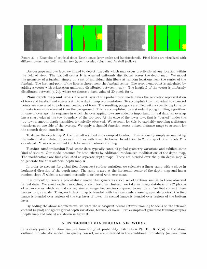
Figure 3. : Examples of artificial data: Depth maps (gray scale) and labels(colored). Pixel labels are visualized withdifferent colors: gap (red), regular tow (green), overlap (blue), and fuzzball (yellow).
Besides gaps and overlaps, we intend to detect fuzzballs which may occur practically at any location withinthe field of view. The fuzzball center F is assumed uniformly distributed across the depth map. We modelthe geometry of a fuzzball simply by a set of individual thin fibers at random locations near the center of thefuzzball. The first end-point of the fiber is chosen near the fuzzball center. The second end-point is calculated byadding a vector with orientation uniformly distributed between [−π, π]. The length L of the vector is uniformlydistributed between [v, 2v], where we choose a fixed value of 30 pixels for v.
Plain depth map and labels The next layer of the probabilistic model takes the geometric representationof tows and fuzzball and converts it into a depth map representation. To accomplish this, individual tow controlpoints are converted to polygonal contours of tows. The resulting polygons are filled with a specific depth valueto make tows more elevated than the background. This is accomplished by a standard polygon filling algorithm.In case of overlaps, the sequence in which the overlapping tows are added is important. In real data, an overlaphas a sharp edge at the tow boundary of the top tow. At the edge of the lower tow, that is ”buried” under thetop tow, a smooth depth transition is typically observed. We account for this by explicitly applying a distancetransform on one side of the overlap. We apply a sigmoid function across a fixed distance range to account forthe smooth depth transition.
To derive the depth map Z, the fuzzball is added at its sampled location. This is done by simply accumulatingthe individual simulated fibers as thin lines with fixed thickness. In addition to Z, a map of pixel labels Y iscalculated. Y serves as ground truth for neural network training.
Further randomization Real sensor data typically contains global geometry variations and exhibits somekind of texture. Our model accounts for both effects by additional randomized modifications of the depth map.The modifications are first calculated as separate depth maps. These are blended over the plain depth map Zto generate the final artificial depth map X.
In order to account for global (low frequency) surface variation, we calculate a linear ramp with a slope inhorizontal direction of the depth map. The ramp is zero at the horizontal center of the depth map and has arandom slope R which is assumed normally distributed with zero mean.
It is difficult to create a probabilistic model that generates a rich set of textures similar to those observedin real data. We avoid explicit modeling of such textures. Instead, we take an image database of 232 photosof urban scenes which we find convey similar image frequencies compared to real data. We first convert theseimages to gray scale. Then, each depth map is blended with two randomly chosen gray-scale photos: the firstimage is blended over regions of the top layer of tows, the second image is blended over regions of the bottomlayer.
By adding the above modifications, we force the subsequent neural network training to focus on the relevantcontent (signal) and ignore global depth variations, texture, or noise. Two examples of generated training samples(depth map and labels) are shown in figure 3.
5. INFERENCE VIA NEURAL NETWORK
It is easily possible to draw samples from the joint probability distribution P(S,F, ...X,Y,Z) of the aboveoutlined probabilistic model. For quality control, we are interested in the conditional probability (or maximum
conv
padding (if required)
upscaling (by factor 2)
padding relu
conv padding relu
De-coding block
vertical input
hori
zont
al in
put
outp
ut
25x37x512
50x75x256 50x75x768
50x75x256
200x300x64
100x150x128
convmax pooling padding relu
conv padding relu
Encoding block
inpu
t
outp
ut
E*200x300x64
200x300x1
E100x150x128
E50x75x256
D
D
100x150x128
conv
200x300x64
200x300x4softmax
E
D50x75x256
25x37x512
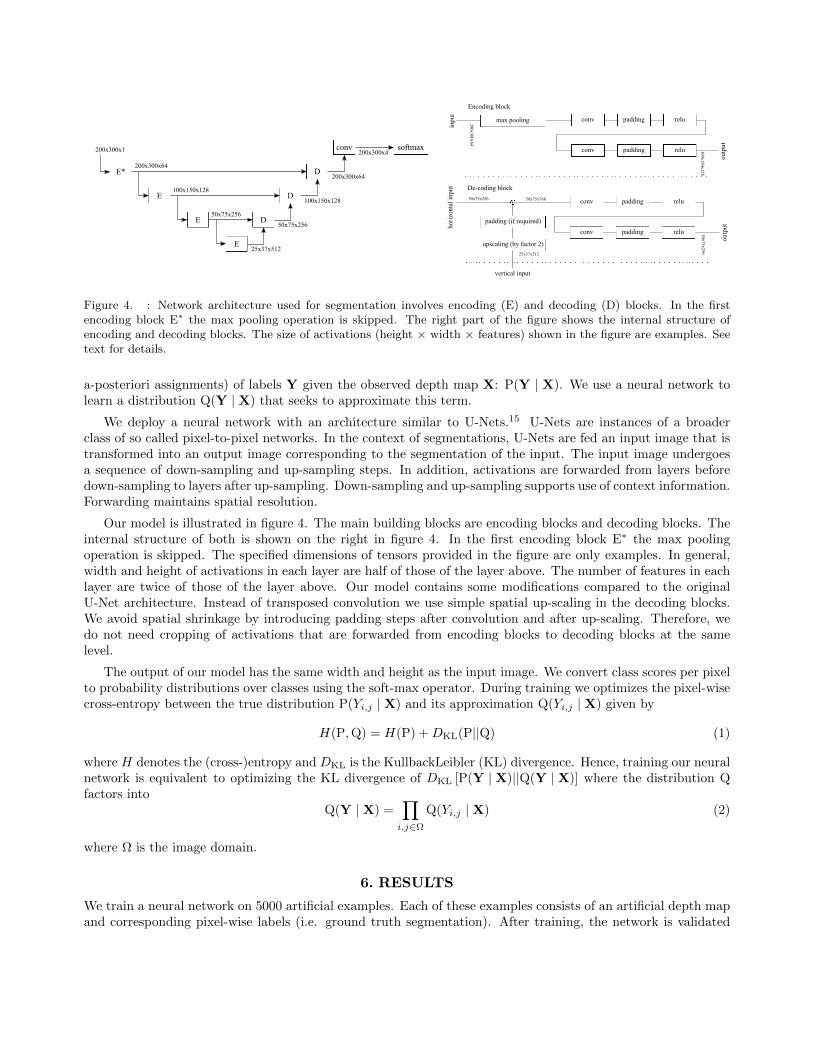
Figure 4. : Network architecture used for segmentation involves encoding (E) and decoding (D) blocks. In the firstencoding block E∗ the max pooling operation is skipped. The right part of the figure shows the internal structure ofencoding and decoding blocks. The size of activations (height × width × features) shown in the figure are examples. Seetext for details.
a-posteriori assignments) of labels Y given the observed depth map X: P(Y | X). We use a neural network tolearn a distribution Q(Y | X) that seeks to approximate this term.
We deploy a neural network with an architecture similar to U-Nets.15 U-Nets are instances of a broaderclass of so called pixel-to-pixel networks. In the context of segmentations, U-Nets are fed an input image that istransformed into an output image corresponding to the segmentation of the input. The input image undergoesa sequence of down-sampling and up-sampling steps. In addition, activations are forwarded from layers beforedown-sampling to layers after up-sampling. Down-sampling and up-sampling supports use of context information.Forwarding maintains spatial resolution.
Our model is illustrated in figure 4. The main building blocks are encoding blocks and decoding blocks. Theinternal structure of both is shown on the right in figure 4. In the first encoding block E∗ the max poolingoperation is skipped. The specified dimensions of tensors provided in the figure are only examples. In general,width and height of activations in each layer are half of those of the layer above. The number of features in eachlayer are twice of those of the layer above. Our model contains some modifications compared to the originalU-Net architecture. Instead of transposed convolution we use simple spatial up-scaling in the decoding blocks.We avoid spatial shrinkage by introducing padding steps after convolution and after up-scaling. Therefore, wedo not need cropping of activations that are forwarded from encoding blocks to decoding blocks at the samelevel.
The output of our model has the same width and height as the input image. We convert class scores per pixelto probability distributions over classes using the soft-max operator. During training we optimizes the pixel-wisecross-entropy between the true distribution P(Yi,j | X) and its approximation Q(Yi,j | X) given by
H(P,Q) = H(P) +DKL(P||Q) (1)
where H denotes the (cross-)entropy and DKL is the KullbackLeibler (KL) divergence. Hence, training our neuralnetwork is equivalent to optimizing the KL divergence of DKL [P(Y | X)||Q(Y | X)] where the distribution Qfactors into
Q(Y | X) =∏
i,j∈Ω
Q(Yi,j | X) (2)
where Ω is the image domain.
6. RESULTS
We train a neural network on 5000 artificial examples. Each of these examples consists of an artificial depth mapand corresponding pixel-wise labels (i.e. ground truth segmentation). After training, the network is validated
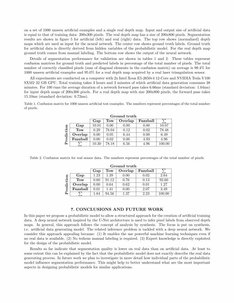
on a set of 1000 unseen artificial examples and a single real depth map. Input and output size of artificial datais equal to that of training data: 200x300 pixels. The real depth map has a size of 200x800 pixels. Segmentationresults are shown in figure 5 for artificial (left) and real (right) data. The top row shows (normalized) depthmaps which are used as input for the neural network. The center row shows ground truth labels. Ground truthfor artificial data is directly derived from hidden variables of the probabilistic model. For the real depth mapground truth comes from manual labeling. The bottom row shows the output of the neural network.
Details of segmentation performance for validation are shown in tables 1 and 2. These tables representconfusion matrices for ground truth and predicted labels in percentage of the total number of pixels. The totalnumber of correctly classified pixels (sum of diagonal elements in the confusion matrix) on average is 99.4% for1000 unseen artificial examples and 95.0% for a real depth map acquired by a real laser triangulation sensor.
All experiments are conducted on a computer with 2x Intel Xeon E5-2650v4 12-Core and NVIDIA Tesla V100SXM2 32 GB GPU. Total training takes 3 hours and 3 minutes of which artificial data generation consumes 38minutes. For 100 runs the average duration of a network forward pass takes 6.66ms (standard deviation: 1.04ms)for input depth maps of 200x300 pixels. For a real depth map with size 200x800 pixels, the forward pass takes15.10ms (standard deviation: 0.72ms).
Table 1. Confusion matrix for 1000 unseen artificial test examples. The numbers represent percentages of the total numberof pixels.
Ground truth
Pre
diction
Gap Tow Overlap Fuzzball∑
Gap 10.01 0.06 0.00 0.00 10.07Tow 0.29 78.04 0.12 0.02 78.48
Overlap 0.00 0.05 6.44 0.00 6.49Fuzzball 0.00 0.02 0.00 4.93 4.96∑
10.30 78.18 6.56 4.96 100.00
Table 2. Confusion matrix for real sensor data. The numbers represent percentages of the total number of pixels.
Ground truth
Pre
diction
Gap Tow Overlap Fuzzball∑
Gap 1.23 1.39 0.00 0.02 2.64Tow 0.60 91.12 0.76 0.13 92.60
Overlap 0.00 0.64 0.62 0.01 1.27Fuzzball 0.01 1.41 0.00 2.07 3.49∑
1.84 94.56 1.37 2.23 100.00
7. CONCLUSIONS AND FUTURE WORK
In this paper we propose a probabilistic model to allow a structured approach for the creation of artificial trainingdata. A deep neural network inspired by the U-Net architecture is used to infer pixel labels from observed depthmaps. In general, this approach follows the concept of analysis by synthesis. The focus is put on synthesis,i.e. artificial data generating model. The related inference problem is tackled with a deep neural network. Weconsider this approach appealing because: (1) It enables the use powerful machine learning techniques even ifno real data is available. (2) No tedious manual labeling is required. (3) Expert knowledge is directly exploitedfor the design of the probabilistic model.
Results so far indicate that segmentation quality is lower on real data than on artificial data. At least tosome extent this can be explained by the fact that the probabilistic model does not exactly describe the real datagenerating process. In future work we plan to investigate in more detail how individual parts of the probabilisticmodel influence segmentation performance. This might help to better understand what are the most importantaspects in designing probabilistic models for similar applications.

Figure 5. : Results of segmentations of unseen artificial data (left) and real data (right). Neural network input (top),ground truth (center), and neural network output (bottom). Pixel labels are visualized with different colors: gap (red),regular tow (green), overlap (blue), and fuzzball (yellow).
ACKNOWLEDGMENTS
Work presented in this paper has received funding from the European Unions Horizon 2020 research and innova-tion programme under grant agreement No 721362 (project ZAero) and by the European Union in cooperationwith the State of Upper Austria within the project Investition in Wachstum und Beschftigung (IWB).
REFERENCES
1. A. Geiger, P. Lenz, and R. Urtasun, “Are we ready for autonomous driving? the KITTI vision benchmarksuite,” in Conference on Computer Vision and Pattern Recognition (CVPR), 2012.
2. M. Johnson-Roberson, C. Barto, R. Mehta, S. N. Sridhar, K. Rosaen, and R. Vasudevan, “Driving in the ma-trix: Can virtual worlds replace human-generated annotations for real world tasks?,” in IEEE InternationalConference on Robotics and Automation (ICRA), pp. 746–753, 2017.
3. F. Mueller, F. Bernard, O. Sotnychenko, D. Mehta, S. Sridhar, D. Casas, and C. Theobalt, “GANeratedhands for real-time 3d hand tracking from monocular RGB,” in IEEE Conference on Computer Vision andPattern Recognition (CVPR), 2018.
4. C. Heindl, S. Zambal, T. Ponitz, A. Pichler, and J. Scharinger, “3d robot pose estimation from 2d images,”The International Conference on Digital Image and Signal Processing , 2019.
5. G. Druck, B. Settles, and A. McCallum, “Active learning by labeling features,” in Conference on EmpiricalMethods in Natural Language Processing: Volume 1, pp. 81–90, Association for Computational Linguistics,2009.
6. B. Settles, “Active learning,” Synthesis Lectures on Artificial Intelligence and Machine Learning 6(1), pp. 1–114, 2012.
7. O. Chapelle, B. Scholkopf, and A. Zien, “Semi-supervised learning (chapelle, o. et al., eds.; 2006)[bookreviews],” IEEE Transactions on Neural Networks 20(3), pp. 542–542, 2009.
8. Z.-H. Zhou, “A brief introduction to weakly supervised learning,” National Science Review 5(1), pp. 44–53,2017.
9. S. J. Pan and Q. Yang, “A survey on transfer learning,” IEEE Transactions on knowledge and data engi-neering 22(10), pp. 1345–1359, 2010.
10. X. Peng, B. Sun, K. Ali, and K. Saenko, “Learning deep object detectors from 3d models,” in IEEEInternational Conference on Computer Vision, pp. 1278–1286, 2015.
11. L. S. Davis, A. Rosenfeld, and J. S. Weszka, “Region extraction by averaging and thresholding,” IEEETransactions on Systems, Man, and Cybernetics (3), pp. 383–388, 1975.
12. A. K. Jain, “Data clustering: 50 years beyond k-means,” Pattern recognition letters 31(8), pp. 651–666,2010.
13. L. Chen, G. Papandreou, I. Kokkinos, K. Murphy, and A. L. Yuille, “Semantic image segmentation withdeep convolutional nets and fully connected CRFs,” in International Conference on Learning Representations(ICLR), 2015.
14. F. Milletari, N. Navab, and S.-A. Ahmadi, “V-net: Fully convolutional neural networks for volumetricmedical image segmentation,” in International Conference on 3D Vision (3DV), pp. 565–571, IEEE, 2016.
15. O. Ronneberger, P. Fischer, and T. Brox, “U-Net: Convolutional networks for biomedical image segmenta-tion,” in International Conference on Medical image computing and computer-assisted intervention, pp. 234–241, Springer, 2015.
16. J. Cemenska, T. Rudberg, and M. Henscheid, “Automated in-process inspection system for afp machines,”SAE International Journal of Aerospace 8(2015-01-2608), pp. 303–309, 2015.
17. P. D. Juarez, K. E. Cramer, and J. P. Seebo, “Advances in in situ inspection of automated fiber placementsystems,” in Thermosense: Thermal Infrared Applications XXXVIII, 9861, p. 986109, International Societyfor Optics and Photonics, 2016.
18. B. Denkena, C. Schmidt, K. Voltzer, and T. Hocke, “Thermographic online monitoring system for automatedfiber placement processes,” Composites Part B: Engineering 97, pp. 239–243, 2016.