INTERNATIONAL INSTITUTE OF TECHNOLOGY & MANAGEMENT, MURTHAL

SONEPAT

E-NOTES

SUBJECT: SURVEYING-2 SUBJECT CODE: -

COURSE- DIPLOMA BRANCH: CIVIL ENGINEERING

SEMESTER 4TH CHAPTER NAME: CONTOUR

(PREPARED BY: Mr. ANKUR CHAUHAN, LECTURER, CE)

1.1 CONTOUR:

An Imaginary line on the ground surface joining the points of equal elevation is

known as contour.

FIG. CONTOUR

1.2 CONTOURING:

The process of tracing contour lines on the surface of the earth is called

Contouring.

1.3 CONTOUR INTERVAL:

The constant vertical distance between two consecutive contours is called the

contour interval.

1.4 HORIZONTAL EQUIVALENT:

The horizontal distance between any two adjacent contours is called as

horizontal equivalent.

FIG. HORIZONTAL EQUIVALENT

1.5 FACTORS AFFECTING CONTOUR

INTERVAL:

Contour interval on a map is decided on the following considerations:

1) Scale of the map

The contour interval is kept inversely proportional to the scale of the map.

Smaller the scale of the map, larger the contour interval. On the other hand, if

the scale of the map is large, the contour interval should be small. If, on a small

scale map, a small contour interval is adopted the horizontal distance between

two consecutive contours i.e. horizontal equivalent, is also small and when

plotted on the scale of the map, the two contours might unite together. It

necessitates to increase the contour interval on small scale maps.

2) Purpose of the map

The contour interval on a map also depends upon the purpose for which the map

is to be utilized. If the map is prepared for setting out a high-way on hills slopes,

a large contour interval might suffice. But, if the map is required for the

construction of an university campus, a small contour interval will be required

for accurate work.

3) Nature of the ground

The contour interval depends upon the general topography of the terrain. In flat

ground, contours at small intervals are surveyed to depict the general slope of

the ground whereas high hills can only be depicted with contours at larger

contour interval. In other words, we may say that the contour interval is

inversely proportional to the flatness of the ground i.e. steeper the terrain, larger

the contour interval.

4) Availability of time and funds

If the time available is less, greater contour interval is adopted to complete the

project in the specified time. On the other hand, if sufficient time is at the

disposal, a smaller contour interval might be decided, keeping in view all the

other factors already described.

1.6 CHARACTERISTICS OF CONTOUR LINES:

Contours show distinct characteristic features of the terrain as follows:

i) All points on a contour line are of the same elevation.

ii) No two contour lines can meet or cross each other except in the rare case of an

overhanging vertical cliff or wall

iii) Closely spaced contour lines indicate steep slope

iv) Widely spaced contour lines indicate gentle slope

v) Equally spaced contour lines indicate uniform slope

vi) Closed contour lines with higher elevation towards the centre indicate hills

vii) Closed contour lines with reducing levels towards the centre indicate pond or

other depression.

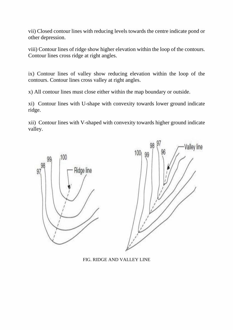
viii) Contour lines of ridge show higher elevation within the loop of the contours.

Contour lines cross ridge at right angles.

ix) Contour lines of valley show reducing elevation within the loop of the

contours. Contour lines cross valley at right angles.

x) All contour lines must close either within the map boundary or outside.

xi) Contour lines with U-shape with convexity towards lower ground indicate

ridge.

xii) Contour lines with V-shaped with convexity towards higher ground indicate

valley.

FIG. RIDGE AND VALLEY LINE

xiii) Contour lines generally do not meet or intersect each other. If contour lines

are meeting in some portion, it shows existence of a vertical cliff.

xiv) Contours of different elevations cannot cross each other. If contour lines

cross each other, it shows existence of overhanging cliffs or a cave.

xv) The steepest slope of terrain at any point on a contour is represented along

the normal of the contour at that point.

xvi) Contours do not pass through permanent structures such as buildings.

1.7 ADVANATAGES OF CONTOUR MAP:

a) For Engineering Works

b) For Military Works.

1.8 METHODS OF CONTOURING

Contouring needs the determination of elevation of various points on the ground

and at the same the horizontal positions of those points should be fixed. To

exercise vertical control levelling work is carried out and simultaneously to

exercise horizontal control chain survey or compass survey or plane table survey

is to be carried out. If the theodolite is used both horizontal and vertical controls

can be achieved from the same instrument. Based on the instruments used one

can classify the contouring in different groups.

However, broadly speaking there are two methods of surveying:

1. Direct methods

2. Indirect methods.

1.8.1 Direct Methods

It consists in finding vertical and horizontal controls of the points which lie on

the selected contour line.

For vertical control levelling instrument is commonly used. A level is set on a

commanding position in the area after taking fly levels from the nearby bench

mark. The plane of collimation/height of instrument is found and the required

staff reading for a contour line is calculated. The instrument man asks staff man

to move up and down in the area till the required staff reading is found. A

surveyor establishes the horizontal control of that point using his instruments.

After that instrument man directs the staff man to another point where the same

staff reading can be found. It is followed by establishing horizontal control.

Thus several points are established on a contour line on one or two contour lines

and suitably noted down. Plane table survey is ideally suited for this work. After

required points are established from the instrument setting, the instrument is

shifted to another point to cover more area. The level and survey instrument

need not be shifted at the same time. It is better if both are nearby so as to

communicate easily. For getting speed in levelling some times hand level and

Abney levels are also used. This method is slow, tedious but accurate. It is

suitable for small areas.

1.8.2 Indirect Methods

In this method, levels are taken at some selected points and their levels are

reduced. Thus in this method horizontal control is established first and then the

levels of those points found. After locating the points on the plan, reduced

levels are marked and contour lines are interpolated between the selected points.

For selecting points anyone of the following methods may be used:

(a) Method of squares,

(b) Method of cross-section, or

(c) Radial line method.

1.8.2.1 Method of Squares: In this method area is divided into a number of

squares and all grid points are marked. Commonly used size of square varies from

5 m × 5 m to 20 m × 20 m. Levels of all grid points are established by levelling.

Then grid square is plotted on the drawing sheet. Reduced levels of grid points

marked and contour lines are drawn by interpolation.

1.8.2.2 Method of Cross-section: In this method cross-sectional points are

taken at regular interval. By levelling the reduced level of all those points are

established. The points are marked on the drawing sheets, their reduced levels

(RL) are marked and contour lines interpolated.

The spacing of cross-section depends upon the nature of the ground, scale of the

map and the contour interval required. It varies from 20 m to 100 m. Closer

intervals are required if ground level varies abruptly. The crosssectional line

need not be always be at right angles to the main line. This method is ideally

suited for road and railway projects.

1.8.2.3 Radial Line Method: Several radial lines are taken from a point in

the area. The of each line is noted. On these lines at selected distances points are

marked and levels determined. This method is ideally suited for hilly areas. In

this survey theodolite with tacheometry facility is commonly used.

1.9 COMPARISION BETWEEN DIRECT AND

INDIRECT METHOD OF CONTOURING:

1.10 Interpolation of contour Interpolation of the contours is the process of spacing the contours

proportionately between the plotted ground points established by indirect

methods. The methods of interpolation are based on the assumption that the slope

of ground between the two points is uniform.

Following are the three methods of interpolation.

• By estimation

• By arithmetic calculation

• By graphical method

By estimation

This method is extremely rough and is used for small scale work only. The

position of contour points between the guide points are located by estimation.

By arithmetic calculation

This method so accurate and is time consuming. The positions of contour points

between the guide points are located by arithmetic calculation e.g. A, B, C and

D be the guide points plotted on the map. Elevations at each point are 607.4,

617.3, 612.5 and 604.3 respectively. Let AB=BD, CD=CA= one inch on plan.

The vertical difference in elevation between A and B is (617.3-607.4) = 9.9 feet.

Hence the distance of the contour points from A will be calculated as follows

i.e., 1/x * y*z

where,

x= Difference in contour elevation between two points

y= The distance between two points

z= The distance between the starting point to contour line

Distance of 610 feet contour point says A1 is calculated by interpolation using

the formula,

The difference in contour elevation between two points is (617.3-607.4) = 9.9

feet.

The distance between the two points = 2.0m

The distance between the starting point to contour line is 610- 607.4 = 2.6 feet

Distance from point ‘A’ is = (1/9.9) x 2.6 x 2 = 0.52 m

1.11 DIFFERENT USES OF CONTOUR MAPS:

• CONTOUR-: An imaginary line on the ground surface joining the equal

elevation is known as contour.

• Contour Map is used in order to select the most economical and suitable

sites.

• It helps to locate the alignments of the canals so that it can follow a ridge

line.

• It helps to mark the alignments of roads and railways so that the quantity

of earthwork both in cutting and filling should be minimum.

• It helps for getting the information about the ground whether it is flat,

undulating or mountainous.

• It helps to find the capacity of reservoir and volume of earthwork especially

in mountainous region.

• It helps us to trace out the given grade of the particular route.

• It helps us to locate the physical features of the ground such as pond

depression, steep or small slopes.

INTERNATIONAL INSTITUTE OF TECHNOLOGY & MANAGEMENT, MURTHAL

SONEPAT

E-NOTES

SUBJECT: SURVEYING-2 SUBJECT CODE: -

COURSE- DIPLOMA BRANCH: CIVIL ENGINEERING

SEMESTER 4TH CHAPTER NAME: THEODOLITE

(PREPARED BY: Mr. ANKUR CHAUHAN, LECTURER, CE)

2.1 THEODOLITE:

Theodolite is a measurement instrument utilized in surveying to determine

horizontal and vertical angles with the tiny low telescope that may move within

the horizontal and vertical planes.

2.1.1 TYPES OF THEODOLITE:

a) TRANSIT THEODOLITE

b) NON- TRANSIT THEODOLITE

• Transit Theodolite: In this type of Theodolite, line of sight can be

reversed by revolving the telescope 180 degrees along the vertical plane.

• Non-Transit Theodolite: In this type of Theodolite, the line of sight

can not be revolved in the vertical plane.

2.1.2 TECHNICAL TERMS OF THEODOLITE:

Vertical axis: It is a line passing through the centre of the horizontal circle and

perpendicular to it. The vertical axis is perpendicular to the line of sight and the

trunnion axis or the horizontal axis. The instrument is rotated about this axis for

sighting different points.

Horizontal axis: It is the axis about which the telescope rotates when rotated

in a vertical plane. This axis is perpendicular to the line of collimation and the

vertical axis.

Telescope axis: It is the line joining the optical centre of the object glass to

the centre of the eyepiece.

Line of collimation: It is the line joining the intersection of the cross hairs to

the optical centre of the object glass and its continuation. This is also called the

line of sight.

Axis of the bubble tube: It is the line tangential to the longitudinal curve of

the bubble tube at its centre.

Centring: Centring the theodolite means setting up the theodolite exactly over

the station mark. At this position the plumb bob attached to the base of the

instrument lies exactly over the station mark.

Transiting: It is the process of rotating the telescope about the horizontal axis

through 180*. The telescope points in the opposite direction after transiting. This

process is also known as plunging or reversing.

Swinging: It is the process of rotating the telescope about the vertical axis for

the purpose of pointing the telescope in different directions. The right swing is a

rotation in the clockwise direction and the left swing is a rotation in the counter-

clockwise direction.

Face-left or normal position: This is the position in which as the sighting

is done, the vertical circle is to the left of the observer.

Face-right or inverted position: This is the position in which as the sighting

is done, the vertical circle is to the right of the observer.

Changing face: It is the operation of changing from face left to face right and

vice versa. This is done by transiting the telescope and swinging it through 180 o

Face-left observation: It is the reading taken when the instrument is in the

normal or face-left position.

Face-right observation: It is the reading taken when the instrument is in the

inverted or face-right position.

2.2 ADJUSTMENT OF A THEODOLITE:

2.2.1. Permanent adjustments:

Plate Levels: The axis of the telescope levels or the altitude level must be parallel

to the line of collimation.

Vertical Circle Index Adjustment: The vertical circle vernier must read zero

when the line of collimation is horizontal.

2.2.2. Temporary Adjustment:

The temporary adjustments are made at each set up of the instrument before we

start taking observations with the instrument. There are three temporary

adjustments of a theodolite:-

i) Centering.

ii) Levelling.

iii) Focussing.

2.3 VERNIER SCALE:

Each theodolite have two scales viz main scale and vernier scale. Main scale is

fixed where as vernier scale is moveable along the edge of main scale.

Vernier scale is a device which is used to observe the fractional part of the

smallest division of the main scale. These vernier one of two types:

(a) Straight vernier scale.

(b) Curved vernier scale.

2.4 MEASUREMENTS OF ANGLES:

1) Horizontal angle measurements

2) Vertical angle measurements

Horizontal angle measurements:

There are three methods of measuring horizontal angles:

1. Ordinary Method. 2. Repetition Method. 3. Reiteration Method.

1. Ordinary Method

To measure horizontal angle AOB:

(i) Set up the theodolite at station-point O and level it accurately.

(ii) Set the vernier A to the zero or 360° of the horizontal circle so do this, loosen

the upper clamp and tum the upper plate until the zero of vernier A nearly

coincides with the zero of the horizontal circle. Tighten the upper clamp and turn

its tangent screw to bring the two zeros into exact coincidence.

(iii) Turn the instrument and direct the telescope approximately to the left hand

object (A) by sighting over the top of the telescope. Tighten the lower clamp and

bisect A exactly by turning the lower tangent screw. Bring the point A into exact

coincidence with the point of intersection of the cross-hairs at diagram by using

the vertical circle clamp and tangent screws.

Alternatively bring the vertical cross-hair exactly on the lowest visible portion of

the arrow or the ranging rod representing the point A in order to minimise the

error due to non- verticality of the object.

(iv) Having sighted the object A, see whether the vernier A still reads zero. This

is done to detect the error caused by turning the wrong tangent screw. Read the

vernier B and record both vernier readings.

(v) Loosen the upper clamp and turn the telescope clockwise until the line of sight

is set nearly on the right hand object (B). Then tighten the upper clamp and by

turning its tangent screw, bisect B exactly. In this operation, the lower clamp and

its tangent screws should not be touched.

(vi) The reading of the vernier A which was initially set at zero gives the value of

the angle AOB directly and that of the other vernier B by deducting 180°. The

mean of the two vernier readings (after deducting 180° from the reading on

vernier B gives the value of the required angle AOB.)

(vii) Change the face of the instrument and repeat the whole process. The mean

of the two vernier readings gives the second value of the angle ABC which should

be approximately or exactly equal to the previous value.

(viii) The mean of the two values of the angle AOB, one with the face left and

the other with the face right, gives the required angle free from all instrumental

errors.

The vernier A is initially set to zero for convenience only. It may be set at any

other reading, and the difference between the initial and the final readings of the

vernier A will give the value of the angle AOB.

2. Repetition Method:

This method is used for very accurate work. In this method; the same angle is

added several times mechanically and the correct value of the angle is obtained

by dividing the accumulated reading by the number of repetitions. The number

of repetitions made usually is six, three with the face left and three with the face

right. In this way, angles can be measured to a finer degree of accuracy than that

obtainable with the least count of the vernier.

However, it cannot be said that any desired degree of accuracy can be obtained

by increasing the number of repetitions considerably because the errors due to

frequent clamping etc. are introduced. There is therefore, no advantage in

increasing the number of observations beyond a certain limit. Three repetitions

with face left and three repetitions with face right are quite sufficient except in

cases of very precise work.

To measure the horizontal angle AOB by repetition:

(i) Set up the theodolite at station -point O and level it accurately. (The face of

the instrument should be left.)

(ii) Set the vernier A to zero or 360° by using the upper clamp and its tangent

screw. Then loosen the lower clamp, direct the telescope to the left hand object

A, and bisect A exactly by using the lower clamp and its tangent screw.

(iii) Check the reading of the vernier A and see whether it still reads zero, and

then read the other vernier B.

(iv) Loosen the upper clamp, turn the telescope clock-wise and bisect the right

hand object (B) exactly by using the upper clamp and its tangent screw.

(v) Read both vernier- The object of reading the vernier is to obtain the

approximate value of the angle. (Suppose the mean reading is 50°4′).

(vi) Loosen the lower clamp and turn the telescope clock-wise until the object (A)

is sighted again. Bisect A accurately using the lower tangent screw. Check the

vernier readings which must be the same as before.

(vii) Loosen the upper clamp, turn the telescope clock-wise and again sight

towards B. Bisect B accurately by using the upper tangent screw.

The vernier will now read twice the value of the angle (It should he approximately

100 °8′).

(viii) Repeat the process until the angle is repeated the required number of times

(usually 3). Read both vernier. The final readings after n repetition should be

approximately n x (50°4′). Divide the sum by the number of repetitions and the

result thus obtained gives the correct value of the angle AOB.

(ix) Change the face of the instrument (now the face will be right). Repeat exactly

in the same manner and find another value of the angle AOB.

(x) The average of the two values of the angle thus obtained gives the required

precise value of the angle (AOB).

The observations are recorded in the tabular form as given in Table.

Errors Eliminated by Measuring the Horizontal Angles by

Repetition:

(i) Errors eliminated by changing face of theodolite:

(a) Error due to the line of collimation not being perpendicular to the horizontal

axis of the telescope.

(b) Error due to the horizontal axis of the telescope not being perpendicular to the

vertical axis.

(c) Error due to the line of collimation not coinciding with the axis of the

telescope.

(ii) Errors eliminated by reading both verniers and averaging the readings:

(a) Error due to the axis of the vernier-plate not coinciding with the axis of the

main scale plate.

(b) Error due to the unequal graduations.

(iii) Error eliminated by measuring the angle on different parts of the

circle:

(a) Error due to unequal graduations.

(iv) The errors in the pointing tend to compensate each other and the remaining

error is minimised by the division.

(v) The error due to dishevelment of the bubble can be minimised by taking

precautions in levelling.

3. Reiteration Method

Reiteration is another precise and comparatively less tedious method of

measuring the horizontal angles. It is generally preferred when several angles are

to be measured at a particular station. This method consists in measuring the

several angles successively, and finally closing the horizon at the starting point.

The final reading of the vernier A should be the same as its initial reading. If not,

the discrepancy is equally distributed among all the measured angles.

Suppose it is required to measure the angles AOB, BOC and COD.

FIG. REITERATION METHOD

Then to measure these angles by reiteration method:

(i) Set up the instrument over station point O and level it accurately.

(ii) Set the vernier A to 0 or 360° by using the upper clamp and its tangent screw.

(iii) Direct the telescope to some well-defined object (P) or say, the station point

A, which is known as the ‘Reference object’. Bisect it accurately by using the

lower clamp and its tangent screw. Check the reading at vernier A which should

still be 0 or 360° and note the reading at vernier B.

(iv) Loosen the upper clamp and turn the telescope clockwise until the point B is

exactly sighted by using the upper tangent screw. Read both verniers. The mean

of the two vernier readings (after deducting 180° from the reading at vernier B)

will give the value of the angle AOB.

(v) Similarly bisect C and D successively, read both verniers at each bisection,

find the values of the angles BOC and COD.

(vi) Finally, close the horizon by sighting towards the reference object (P) or the

station-point A.

(vii) The vernier A should now read 360°. If not, note down the error. This error

occurs due to slip etc.

(viii) If the error is small, it is equally distributed among the several observed

angles. If large, the readings should be discarded and a new set of readings be

taken.

(ix) Change the face of the instrument.

(x) Set the vernier A to a reading other than 0°, say, 60° or 90°. This is done to

avoid errors of graduation.

(xi) Again measure the angles in the same manner by turning the telescope this

time in the counter-clockwise direction to compensate or slip and errors due to

twisting of the instrument.

(xii) Close the horizon and apply the necessary correction to all the angles as

before.

(xiii) The mean of the two results for each angle is taken as its true value.

2.5 MEASUREMENT OF VERTICAL ANGLES:

Vertical Angle: A vertical angle is an angle between the inclined line of sight

and the horizontal. It may be anangle of elevation or depression according as the

object is above or below the horizontal plane.

MEASUREMENT OF VERTICAL ANGLES:

To Measure the Vertical Angle of an object A at a station O:

(i) Set up the theodolite at station point O and level it accurately with reference

to the altitude bubble.

(ii) Set the zero of vertical vernier exactly to the zero of the vertical circle clamp

and tangent screw.

(iii) Bring the bubble of the altitude level in the central position by using clip

screw. The line of sight is thus made horizontal and vernier still reads zero.

(iv) Loosen the vertical circle clamp screw and direct the telescope towards the

object A and sight it exactly by using the vertical circle tangent screw.

(v) Read both vernier on the vertical circle, the mean of the two vernier readings

gives the value of the required angle.

(vi) Change the face of the instrument and repeat the process. The mean of the

two vernier readings gives the second value of the required angle.

(vii) The average of the two values of the angles thus obtained, is the required

value of the angle free from instrumental errors.

For measuring Vertical Angle between two points A &B

i) Sight A as before, and take the mean of the two vernier readings at the vertical

circle. Let it be α.

ii) Similarly, sight B and take the mean of the two vernier readings at the vertical

circle.

iii) The sum or difference of these dings will give the value of the vertical angle

between A and B according as one of the points is above and the other below the

horizontal plane. or both points are on the same side of the horizontal plane

2.6 PROLONGING A STRAIGHT A LINE

There are two methods of prolonging a given line such as AB

(1) Fore sight method, and (2) Back Sight Method

(1) Fore Sight Method: As shown in the fig. below

i) Set up the theodolite at A and level it accurately. Bisect the point b correctly.

Establish a point C in the line beyond B approximately by looking over the top

of the telescope and accurately by sighting through the telescope.

ii) Shift the instrument to B ,take a fore sight on C and establish a point D in line

beyond C.

iii) Repeat the process until the last point Z is reached.

FIG. FORE SIGHT METHOD

(2) Back Sight Method: As shown in the fig. below

i) Set up the instrument at B and level it accurately.

ii) Take a back sight on A.

iii) Tighten the upper and lower clamps, transit the telescope and establish a point

C in the line beyond B.

iv) Shift the theodolite to C, back sight on B transit the telescope and establish a

point D in line beyond C. Repeat the process until the last point (Z) is established.

FIG. BACK SIGHT METHOD

2.7 Finding Height of an Object Using a Theodolite

There may be two cases to find height of an object using a theodolite:

1. When the base of the object is accessible.

2. When the base of the object is inaccessible.

2.7.1. Base of the Object being Accessible:

To find the height of the object above a Bench Mark:

Let H = the height of the object above the B.M.

h = the height of the object above the instrument axis.

hs = height of the instrument axis above the B.M.

α = the vertical angle observed at the instrument-station.

D = the horizontal distance in metres measured from the instrument-station to the

base of the object.

Then, h = D tan α

H = h + hs = D tan α + hs

When the distance D is large, the correction for curvature and refraction,

viz. shall have to be applied.

If the height of the object above the instrument-station is to be found out, then

add the height of the instrument axis to the height of the object above the

instrument axis. The height of the instrument axis may be obtained in two ways.

(i) By measuring the height of centre of the eye-piece above the station point by

a steel tape.

(ii) By readings the staff through the object-glass when held just near the eye-

piece end.

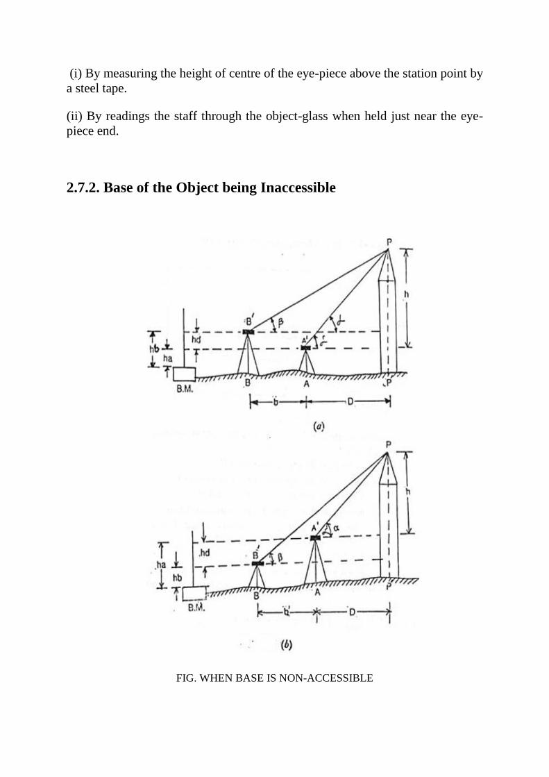
2.7.2. Base of the Object being Inaccessible

FIG. WHEN BASE IS NON-ACCESSIBLE

To find the height of the object above a bench mark (B.M.):

(i) Choose two stations A and B suitable on a fairly level ground so that they lie

in a vertical plane passing through the object in line with the object, and measure

the distance between them accurately.

(ii) Set up the instrument over the station. A and level it accurately.

(iii) With the altitude bubble central and with the vertical vernier reading zero,

take a reading on the staff held on the B.M. or reference point.

(iv) Bisect the object P and read both verniers. Change the face, again sight P and

read both verniers, Take mean of the four readings, which is the correct value of

the vertical angle.

(v) Shift the instrument to B and take similar observations as at A.

Let α = the angle of elevation observed at A.

β = the angle of elevation observed at B.

b = the horizontal distance between the instrument-stations A and B.

D = the distance of the object from the near station.

h = height of the object P above instrument axis at A’.

ha =the staff reading at the B.M. when the instrument is at A.

hb = the staff reading at the B.M. when the instrument is at B.

hd = the level difference between the two positions of the instrument axis.

= ha – hb

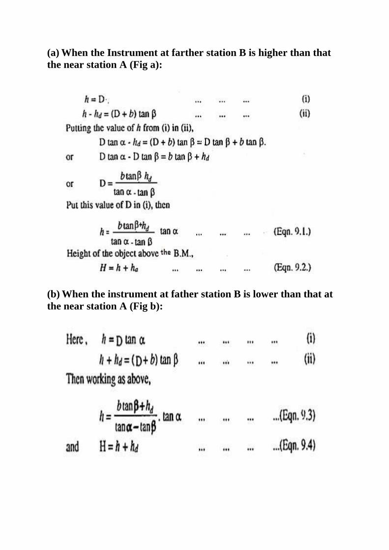
(a) When the Instrument at farther station B is higher than that

the near station A (Fig a):

(b) When the instrument at father station B is lower than that at

the near station A (Fig b):

2.8 Theodolite traverse

A traverse is a series of connected lines whose lengths and directions measures

in the field. In a theodolite traverse, to directions measured with a theodolite. A

theodolite traverse in commonly used for providing a horizontal control system

to determine the relative positions of the various points on the surface of the earth.

It especially uses for providing control for site surveys in urban areas where the

triangulation is not feasible.

The equipment required for conducting a theodolite traverse will include a

theodolite, a steel tape, two ranging poles, stakes, tacks, plumb bobs, chain pins,

tripods, crayons, makers, an ax and a hammer. The traverse may be an open

traverse or a closed traverse. A closed traverse commonly uses in control survey,

construction survey, property survey, and topographic survey.

2.9 Theodolite traversing

In this type of traversing, traverse legs measures by direct chaining on the ground

the traverse angles at every traverse stations measures accurately with a

theodolite.

The basic procedure for theodolite traversing is the same as that in any other

method of traversing. First reconnaissance has to conducted with a sketch drawn

the terrain using the approximate location of traverse station then the important

details are to pick up, the inter visibility of station to check. Theodolite traversing

required station marking tools such as pegs. arrows, etc., a theodolite with its

stand and steel tape.

2.10 ERRORS IN THEODOLITE SURVEYING:

The Errors in theodolite surveying may be grouped into following three, based

on their sources:

i) Instrumental

ii) Natural

iii) Personal

2.10.1 Instrumental Errors:

(i) Non-adjustment of plate levels:

If the plate levels which are not perpendicular to the vertical axis, are centered,

the vertical axis of the instrument is not made truly vertical. As a result, the

horizontal circle is inclined and the angles are measured in an inclined plane

instead of in a horizontal plane.

The errors are introduced in the measurements of both horizontal and vertical

angles. The error is serious when the horizontal angles between points at

considerably different elevations are to be measured.

The error can be minimised by levelling the instrument with reference to the

altitude bubble.

(ii) The line of collimation not being perpendicular to the horizontal axis:

If the line of collimation is not perpendicular to the horizontal axis, it will trace

out the surface of a cone instead of a plane when the telescope is revolved in the

vertical plane. As a result, horizontal angles when measured between points at

widely different elevations will be incorrect.

The error can be eliminated by reading angles on both the faces and taking the

mean of the observed values.

(iii) The horizontal axis not being perpendicular to the vertical axis:

If the horizontal axis is not perpendicular to the vertical axis, the line of

collimation will not revolve in a vertical plane when the telescope is raised or

lowered. This causes an angular error both in horizontal and vertical angles.

The error can be eliminated by reading angles on both the faces and taking the

mean of the two values.

(iv) The line of collimation and the axis of telescope-level not being parallel

to each other:

If the line of collimation and the axis of telescope- level are not parallel to each

other, the zero line of the vertical vernier is not a true line of reference and as a

result, an error is introduced in the measurement of vertical angles.

The error can be eliminated by taking two observations of the angles, one with

the telescope normal and the other with the telescope inverted, and taking the

mean of the two values.

(v) The inner and outer axis i.e. the axes of both the upper and lower plates

not being concentric:

This makes the angles read on cither vernier incorrect.

The error is eliminated by reading both vernier and averaging the two values.

(vi) The graduations being unequal:

The error is minimised by measuring the angles several times on different parts

of the circle and taking the mean of all.

(vii) Vernier being eccentric:

The zeros of the vernier will not be diametrically opposite to each other. An error

will be introduced if only one vernier is read, but it will cancel itself if both

vernier are read and the mean taken.

(viii) The vertical hair not being exactly vertical:

The error is minimised by using the portion of the hair near the horizontal hair

for bisecting the signal.

2.10.2 Observational or Personal Errors:

(i) Inaccurate Centering:

This is very common error and is introduced in all angles measured at a given

station. Its magnitude depends upon the length of the sight. It varies inversely as

the length.

The error is much reduced by carefully centering the instrument over the station-

mark.

(ii) Inaccurate Levelling:

The effect of this error is similar to that of the error due to non-adjustment of plate

levels. The error is serious when horizontal angles between points at considerably

different elevations are to be measured.

The error can be minimised by levelling the instrument carefully with reference

to the altitude level.

(iii) Slip:

The slip may occur if the instrument is not firmly screwed to the tripod-head or

the shifting head is not sufficiently clamped or the lower clamp is not properly

tightened. As a result, the observations will be in error. This can be prevented by

proper care.

(iv) Working wrong tangent screw:

This is a common mistake on the part of a beginner. This can be avoided by proper

care and experience. Always operate the lower tangent screw for a back sight and

the upper tangent screw for a foresight.

(v) Parallax:

This error arises due to imperfect focussing. The parallax can be eliminated by

properly focussing the eye-piece and the object-glass.

(vi) Inaccurate bisection of the point sighted and non-verticality of the

ranging rod:

Care should be taken to bisect the lowest point visible on the ranging rod. In case

of short sights, the point of a pencil or the blub- line may be used instead of a

ranging rod. The error varies inversely with the length of sight.

(vii) Other errors such as:

(a) Mistake in setting the vernier,

(b) Mistake in reading the scales and vernier,

(c) Mistake in reading wrong vernier, and

(d) Mistake while booking the readings can be prevented by habitual checks and

precautions.

2.10.3 Natural Errors:

These errors are due to:

(i) High temperature causing irregular refraction,

(ii) Wind storm causing vibration of the instrument,

(iii) The sun shining on the instrument, etc.

These are negligible for ordinary surveys.

But the precise work is usually performed under the most favourable atmospheric

conditions.

INTERNATIONAL INSTITUTE OF TECHNOLOGY & MANAGEMENT, MURTHAL

SONEPAT

E-NOTES

SUBJECT: SURVEYING-2 SUBJECT CODE: -

COURSE- DIPLOMA BRANCH: CIVIL ENGINEERING

SEMESTER 4TH CHAPTER NAME: TACHEOMETRY

(PREPARED BY: Mr. ANKUR CHAUHAN, LECTURER, CE)

3.1 TACHEOMETRY:

Tacheometric surveying (also called stadia surveying) is a rapid and economical

surveying method by which the horizontal distances and the differences in

elevation are determined indirectly using intercepts on a graduated scale and

angles observed with a transit or the theodolite.

3.2 DIFFERENT INSTRUMENTS USED IN TACHEOMETRY.

The following are the two main instruments:

(a) Tacheometer

(b) Stadia rod.

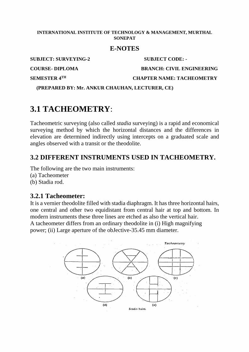
3.2.1 Tacheometer: It is a vernier theodolite filled with stadia diaphragm. It has three horizontal hairs,

one central and other two equidistant from central hair at top and bottom. In

modern instruments these three lines are etched as also the vertical hair.

A tacheometer differs from an ordinary theodolite in (i) High magnifying

power; (ii) Large aperture of the obJective-35.45 mm diameter.

3.2.2 Stadia rod For short distances an ordinary levelling staff with 5 mm graduation can be used.

For long distances, a special large staff called a stadia rod is used. It is usually

3 to 5 m long and in one piece. The width is between 50 to 150 mm. The

graduations are very prominent so that they can be read from long distances.

3.3 DIFFERENT METHODS OF TACHEOMETRY: There are basically three types of tacheometric measurements.

1. Stadia system which again can be divided into-

(i) Fixed hair method,

(ii) Movable hair method.

2. Tangential system.

3. Subtense bar system.

In the fixed hair method, as the name suggests, the hairs are fixed in position.

i.e. the distance between them remains constant, The staff intercepts. i.e. the

readings at which the hairs intersect the staff varies as the distance of the staff

from the instrument station varies.

In the movable hair method. as the 'name suggests. the stadia hairs; i.e. the'

top and bottom hairs are movable and this is done by means of micrometer

screws. The staff intercept ·S·. however. is kept fixed at' a constant spacing of

usually 3 m. While taking readings at different distances micrometer screws are

adjusted such that the top and bottom hairs intersect the fixed targets. As it is

difficult to measure the stadia interval accurately and adjust the stadia hair every

time an observation is to be taken. this method is rarely used. On the other hand,

the fixed hair method is frequently used.

In the tangential systems. the stadia hairs are not essential. However, two

readings are to be taken at the two targets at a fixed distance 'S' apart in the

staff.

In the subtense bar system a special staff with two targets at two ends at a

fixed distance apart known as subtense bar is placed horizontally and the angle

between the targets from the Instrument station is measured. This is shown in

Fig. where plan view of the subtense bar is shown.

3.4 STADIA METHOD: The Stadia is a method of measuring distances rapidly with a telescope (usually

on an engineer's transit or an alidade) and a graduated rod. ... If the line of sight

is inclined, the vertical angle is also measured and can be used to reduce the

results to horizontal and vertical distances.

3.4.1 General Principle of Stadia Tacheometry:

Let O= the optical center of the object – glass

a, b and c= the bottom, top and central hairs at diagram

A, B and C= the points on the staff cut by the three lines

a b = i the interval between stadia lines.

(ab is the length of the image of AB)

AB=S=the staff intercept (the differences of the stadia hair readings)

f= the focal length of object – glass i.e. the distance between the centre (O) to the

principal focus (FG) of the lens.

u – the horizontal distance from the optical centre (O) to the staff.

v = the horizontal distance from the optical centre (O) to the image of the staff, u

and v being called the conjugate focal length of the lens.

d = the horizontal distance form optical centre (O) to the vertical axis of the

tacheometer.

D = the horizontal distance from the vertical axis of the instrument to the staff,

The constant f/i is called the multiple constant and its value is usually 100, while

the constant (f+d) is called the additive constant and its value varies from 30 cm

to 60 cm in case of external focussing telescope, it is very small varying from 10

cm to 20 cm and is therefore ignored.

To make the value of additive constant zero, an additional convex lens, known as

lens, is provided in the telescope between the object – glass and eye piece at a

fixed distance from former. By this arrangement, calculation work is reduced

considerably.

The equation 10.1 is applicable only when the line of sight is horizontal and the

staff is held vertical.

3.4.2 Determination of Stadia Constants of a Tacheometer:

There are two methods available for finding the values of the stadia constant f/i

and f + d of a given instrument.

First method:

In this method, the values of the constants are obtained by the computations

form the field measurements.

Procedure:

(i) Measure accurately a line OA about 300 m long, on a fairly level ground and

fix pegs along it at intervals of say, 30m.

(ii) Set up the instrument at O and obtained the staff intercepts by taking stadis

reading on the staff held vertically at each of the pegs.

On substituting the values of D and S in the Equations 10.1, we get a

number of equations which when solved in pairs, give the several values of

the constants:

their mean value being adopted to the values of the constants. Thus, if D1,D2, D3,

etc.=the distances measured from the instrument, and S1, S2, S3 etc.= the

corresponding staff intercepts.

Then we have:

Second Method:

In this method, the value of the multiplying constant f/i is found by computations

from the field measurements and that of the additive constant (f+) is obtained by

the direct measurements at the telescope.

Procedure:

(i) Sight any far distant – object and focus it.

(ii) Measure accurately the distance along the top of the telescope between the

object -Glass and the plane of the cross -hairs (diagram screw) with a rule, the

measured distance being equal to the focal length (f) of the objective.

(iii) Measure the distance (d) from the object— glass to the vertical axis of the

instrument.

(iv) Measure several lengths D1, D2, D3 etc. along OA from the instrument –

position O and obtained the staff intercepts S1, S2, S3 ate. at each of these lengths.

(v) Add f and d find the values of the additive constant (f+d).

(vi) Knowing (f+d), determined the several values of f/i from the equation 10. 1.

(vii) The mean of the several values gives the required value of the multiple

constant f/i. Calculation work is much simplified, of the instrument is placed at a

distance of (f+d) beyond the beginning O of the line.

Note:

The value of the additive constant in case of an internal focussing telescope

cannot be determined in this way. One has to depend upon the value supplied by

the maker.

3.4.3 Theory of Anallatic Lens:

An additional convex lens, called an anallatic lens, is provided in the external focussing

telescope between the eye — piece and the object — glass at a fixed distance from the

later, to eliminate the additive constant, (f+d), from the distance formula:

in order to simplify the calculation work. The anallatic lens is seldom placed in

the internal focussing telescope since the value of the additive constant is only a

few centimeters and can be neglected. The disadvantage of the anallatic a lens is

the reduction in brilliancy of the image due to increase observation of light.

The value of the additive constant, (δ+d) can be made equal to zero by bringing

the apex (G) of the tacheometric angle AGB (Fig) into exact coincidence with the

centre on\f the instrument.

The theory of anallatic lens is explained ad follows:

In fig.

Let, S = the staff intercept AB.

i = the length b a of the image of AB i.e. the actual stadia interval when the

anallatic lens is interposed.

i = the length ba of the image of AB when no anallatic lens was provided.

O = the optical centre of the object – glass.

O = the optical centre of the anallatic lens

e = the distance between the optical centre of the object glass and the anallatic

lens.

f = to length of object glass.

f’ = focal length of the anallatic lens.

F = Principle focus of the anallatic lens.

G = the centre of the instrument.

d = the distance from the centre of the object — glass top the vertical axis of the

instrument.

D – the distance from the vertical axis of the instrument to the staff.

f1and f2 = the conjugate focal length of the object —glass.

k = the distance from the optical centre of the object glass to the actual image b

a.

(k— e) and (f2 —e) = the conjugate focal length of the anallatic lens.

The ray of light from A and B are refracted by the object — glass to meet at F.

The anallatic lens is so placed that F is its principal focus. Thus ray of light would

become parallel to the axis of the telescope after passing through the anallatic

lens and give actual image b a of the staff intercept AB.

The negative sign is used in (ii) since b ‘a’ and ba are on the same side of the

anallatic lense.

now the conditions that D should be proportional to S requires that the 2nd and

3rd terms in (v) are equal to zero so that

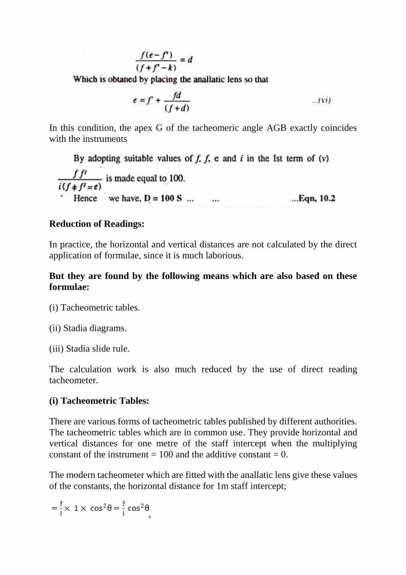
In this condition, the apex G of the tacheomeric angle AGB exactly coincides

with the instruments

Reduction of Readings:

In practice, the horizontal and vertical distances are not calculated by the direct

application of formulae, since it is much laborious.

But they are found by the following means which are also based on these

formulae:

(i) Tacheometric tables.

(ii) Stadia diagrams.

(iii) Stadia slide rule.

The calculation work is also much reduced by the use of direct reading

tacheometer.

(i) Tacheometric Tables:

There are various forms of tacheometric tables published by different authorities.

The tacheometric tables which are in common use. They provide horizontal and

vertical distances for one metre of the staff intercept when the multiplying

constant of the instrument = 100 and the additive constant = 0.

The modern tacheometer which are fitted with the anallatic lens give these values

of the constants, the horizontal distance for 1m staff intercept;

,

and vertical distances for 1m staff intercept

The tables provided these values for different values of varying from 0° to 30°

For example, suppose, the vertical angle is 3° 20^ and the staff intercept is 1.70m.

From the tables, it is seen that horizontal and vertical distance for 1 metre staff in

percept i.e.

Thus for 1.70m staff intercept, the horizontal distance = 1.70 x 99 .67 – 169.439

m and the vertical distance = 1.70 x 5.80 = 9.86 m.

(ii) Stadia Diagrams:

The stadia diagrams show graphically the quantities

The diagram are available in different forms but surveyors often prepare these

diagrams of their own design. The use of stadia diagram is consider faster than

the use of tables but can be used for ordinary distance.

(iii) Stadia Slide Rule:

The horizontal and vertical distances are computed conveniently by stadia slide

rule. Stadia slide rules are available in different patterns but the one in common

use is constructed like the ordinary slide rule, except that on the slide rule are

given values of cos2 and 1/2 sin 2, these qualities being plotted to a log scale. The

stadia slide rule is equally suitable for the field or office work.

3.5 Uses of Stadia The stadia method of surveying is particularly useful for following cases: 1. In differential leveling, the back sight and foresight distances are balanced conveniently if the level is equipped with stadia hairs.

2. In profile leveling and cross sectioning, stadia is a convenient means of finding distances from level to points on which rod readings are taken.

3. In rough trigonometric, or indirect, leveling with the transit, the stadia method is more rapid than any other method.

4. For traverse surveying of low relative accuracy, where only horizontal angles and distances are required, the stadia method is a useful rapid method. 5. On surveys of low relative accuracy - particularly topographic surveys-where both the relative location of points in a horizontal plane and the elevation of these points are desired, stadia is useful. The horizontal angles, vertical angles, and the stadia interval are observed, as each point is sighted; these three observations define the location of the point sighted.

3.6 Errors in Stadia Surveying:

The sources of errors in stadia measurements are as follows:

1. Instrumental Errors.

2. Personal Errors.

3. Natural Errors.

3.6.1. Instrumental Errors:

(i) Imperfect adjustment of the tacheometer:

This error can be eliminated by carefully adjusting the instrument, particularly

the altitude bubble.

(ii) Incorrect divisions on the stadia rod:

In ordinary work, this error is negligible but for precise work, the error can be

minimised by using the standardised rod and applying corrections for incorrect

length to the observed stadia intervals.

(iii) Incorrect value of the multiplying constant (f/t):

This is the most serious source of error. The value of the multiplying constant

should be tested before commencing the work by comparing the stadia distances

with measured distances during the hours which correspond to those of field-

observations.

3.6.2. Personal Errors:

(i) Inaccurate centering and levelling of the instrument.

(ii) Non-vertical by of the staff or rod. It may be eliminated by using a plumb-

line or a small circular spirit level with the staff.

(iii) Inaccurate Focussing.

(iv) Reading with wrong hair.

The personal errors can be eliminated by applying habitual checks.

3.6.3. Natural Errors:

(i) High wind:

The work should be suspended in high wind.

(ii) Unequal refractions:

This error is prominent during bright sunshine and mid-day hours of hot summer

days. The work can be suspended under such circumstances.

(iii) Unequal expansion:

The instrument should be protected by an umbrella during hot sun.

(iv) Bad visibility:

It is caused by glaring of strong light coming from the wrong direction.

Degree of Accuracy:

The error in a single horizontal distance should not exceed 1 in 500, and in a

single vertical distance 0.1 m.

Average error in distance varies from the 1 m 600 to 1 in 850.

Error of closure in elevation varies from 0.08 √km to 0.25 √km where km =

distance in km. error of closure in a stadia traverse should not exceed 0.055 √P

metres, where P = perimeter of the traverse in metres.

INTERNATIONAL INSTITUTE OF TECHNOLOGY & MANAGEMENT, MURTHAL

SONEPAT

E-NOTES

SUBJECT: SURVEYING-2 SUBJECT CODE: -

COURSE- DIPLOMA BRANCH: CIVIL ENGINEERING

SEMESTER 4TH CHAPTER NAME: CURVES

(PREPARED BY: Mr. ANKUR CHAUHAN, LECTURER, CE)

4.1 CURVES:

IT IS GRADUAL CHANGE OF DIRECTION EITHER IN HORIZONTAL OR

VERTICAL PLANE.

The center line of a road consists of series of straight lines interconnected by

curves that are used to change the alignment, direction, or slope of the road.

Those curves that change the alignment or direction are known as horizontal

curves, and those that change the slope are vertical curves.

The initial design is usually based on a series of straight sections whose

positions are defined largely by the topography of the area. The intersections of

pairs of straights are then connected by horizontal curves. Curves can be listed

under three main headings, as follows:

(1) Horizontal curve

(2) Vertical curves

4.1.1 Horizontal Curves When a highway changes horizontal direction, making the point where it

changes direction a point of intersection between two straight lines is not

feasible. The change in direction would be too abrupt for the safety of modem,

high-speed vehicles. It is therefore necessary to interpose a curve between the

straight lines. The straight lines of a road are called tangents because the lines

are tangent to the curves used to change direction.

The smaller the radius of a circular curve, the sharper the curve. For modern,

high-speed highways, the curves must be flat, rather than sharp. The principal

consideration in the design of a curve is the selection of the length of the radius

or the degree of curvature. This selection is based on such considerations as the

design speed of the highway and the sight distance as limited by headlights or

obstructions

4.1.2 Types of Horizontal Curves There are four types of horizontal curves. They are described as follows:

A. Simple. The simple curve is an arc of a circle (view A, fig. 1). The radius of

the circle determines the sharpness or flatness of the curve.

B. Compound. Frequently, the terrain will require the use of the compound

curve. This curve normally consists of two simple curves joined together and

curving in the same direction (view B, fig. 1).

C. Reverse. A reverse curve consists of two simple curves joined together, but

curving in opposite direction. For safety reasons, the use of this curve should be

avoided when possible (view C, fig. 1).

D. Spiral. The spiral is a curve that has a varying radius. It is used on railroads

and most modem highways. Its purpose is to provide a transition from the

tangent to a simple curve or between simple curves in a compound curve.

FIGURE 1

4.1.3 Elements of Horizontal Curves The elements of a circular curve are shown in figure 2. Each element is

designated and explained as follows:

Point of Intersection (PI). The point of intersection is the point where the back

and forward tangents intersect. Sometimes, the point of intersection is

designated as V (vertex).

Deflection Angle. The central angle is the angle formed by two radii drawn

from the center of the circle (O) to the PC and PT. The value of the central

angle is equal to the I angle. Some authorities call both the intersecting angle

and central angle either I or A.

Radius (R). The radius of the circle of which the curve is an arc, or segment.

The radius is always perpendicular to back and forward tangents.

Point of Curvature (PC). The point of curvature is the point on the back

tangent where the circular curve begins. It is sometimes designated as BC

(beginning of curve) or TC (tangent to curve).

Station P.C.= P.I. – T

Point of Tangency (PT), The point of tangency is the point on the forward

tangent where the curve ends. It is sometimes designated as EC (end of curve)

or CT (curve to tangent).

Station P.T. = P.C.+ L

Point of Curve. The point of curve is any point along the curve.

Length of Curve (L). The length of curve is the distance from the PC to the PT,

measured along the curve.

Tangent Distance (T). The tangent distance is the distance along the tangents

from the PI to the PC or the PT. These distances are equal on a simple curve.

Long Cord (C). The long chord is the straight-line distance from the PC to the

PT. Other types of chords are designated as follows:

C The full-chord distance between adjacent stations (full, half, quarter, or one

tenth stations) along a curve.

C1 The sub chord distance between the PC and the first station on the curve.

External Distance (E). The external distance (also called the external secant) is

the distance from the PI to the midpoint of the curve. The external distance

bisects the interior angle at the PI.

Middle Ordinate (M). The middle ordinate is the distance from the midpoint of

the curve to the midpoint of the long chord. The extension of the middle

ordinate bisects the central angle.

Degree of Curve. The degree of curve defines the sharpness or flatness of the

curve.

FIGURE 2

4.2 CIRCULAR CURVES

A simple circular curve shown in Fig, consists of simple arc of a circle of radius

R connecting two straights AI and IB at tangent points T1 called the point of

commencement (P.C.) and T2 called the point of tangency (P.T.), intersecting at

I, called the point of intersection (P.I.), having a deflection angle or angle of

intersection. The distance E of the midpoint of the curve from I is called the

external distance. The arc length from T1 to T2 is the length of curve, and the

chord T1T2 is called the long chord. The distance M between the midpoints of

the curve and the long chord, is called the mid-ordinate. The distance T1I which

is equal to the distance IT2, is called the tangent length. The tangent AI is called

the back tangent and the tangent IB is the forward tangent.

Methods of Setting out of single Circular curve

• Two Methods

• 1) Linear Methods

• 2) Angular Methods.

• 1) Linear Methods

• ‐ (i) By offsets or ordinate from the long chord.

• (ii) By successive bisection of arcs or chords.

• (iii) By offsets from the tangents.

• (iv) By offsets from the chord produced.

4.3 Transition Curves: A non-round bend of fluctuating range presented between a straight and a

roundabout bend to give simple alters of course of a course is known as a progress

or easement bend. It is additionally embedded between two parts of a compound

or switch bend.

Points of interest of giving a progress bend at each finish of a round bend:

(i) The change from the digression to the round bend and from the roundabout

bend to the digression is made progressive.

(ii) It gives acceptable methods for acquiring a continuous increment of super-

rise from zero on the digression to the required full sum on the fundamental

roundabout bend.

(iii) Danger of crash, side sliding or upsetting of vehicles is wiped out.

(iv) Discomfort to travelers is killed.

Conditions to be satisfied by the change bend:

(i) It should meet the digression line just as the roundabout bend extraneously.

(ii) The rate of increment of shape along the change bend ought to be equivalent

to that of increment of super-height.

(iii) The length of the change bend ought to be to such an extent that the full

super-rise is accomplished at the intersection with the round bend.

(iv) Its span at the intersection with the roundabout bend ought to be equivalent

to that of round bend.

There are three kinds of change bends in like manner use:

(1) A cubic parabola,

(2) A cubical winding, and

(3) A lemniscate, the initial two are utilized on railroads and parkways both, while

the third on roadways as it were.

At the point when the progress bends are presented at each finish of the primary

roundabout bend, the blend along these lines got is known as consolidated or

Composite Curve.

4.4 Super-Elevation or Cant:

At the point when a vehicle goes from a straight to a bend, it is followed up on

by an outward power notwithstanding its own weight, both acting through the

focal point of gravity of the vehicle. The diffusive power acts on a level plane and

will in general push the vehicle off the track.

So as to neutralize this impact the external edge of the track is too raised or raised

over the inward one. This raising of the external edge over the internal one is

called super rise or cant. The measure of super-height relies on the speed of the

vehicle and sweep of the bend.

Super elevation

Let:

W = the heaviness of vehicle acting vertically downwards.

F = the divergent power acting on a level plane,

v = the speed of the vehicle in meters/sec.

g = the speeding up because of gravity, 9.81 meters/sec2.

R = the span of the bend in meters,

h = the super-height in meters.

b = the expansiveness of the street or the separation between the focuses of the

rails in meters.

At that point for harmony, the resultant of the weight and the outward power

ought to be equivalent and inverse to the response opposite to the street or rail

surface.

4.4.1 Characteristics of a Transition Curve:

Here two straights AB and BC make a redirection edge ∆, and a roundabout

bend EE' of sweep R, with two change, bends TE and E'T' at the two closures,

has been embedded between the straights.

(I) It is obvious from the assume that so as to fit in the progress bends at the

finishes, around fanciful bend (T1F1T2) of marginally more prominent range

must be moved towards the middle as(E1 EF E E1. The separation through

which the bend is moved is known as move (S) of the bend, and is equivalent to,

where L is the length of each change bend and R is the range of the ideal round

bend (EFE'). The length of the move (T1E1) and the change bend (TE)

commonly separate one another.

INTERNATIONAL INSTITUTE OF TECHNOLOGY & MANAGEMENT, MURTHAL

SONEPAT

E-NOTES

SUBJECT: SURVEYING-2 SUBJECT CODE: -

COURSE- DIPLOMA BRANCH: CIVIL ENGINEERING

SEMESTER 4TH CHAPTER NAME: MODERN INSTRUMENTS

(PREPARED BY: Mr. ANKUR CHAUHAN, LECTURER, CE)

5.1 ELECTRONICS DISTANCE MEASUREMENT (EDM)

EDM is a general term embracing the measurement of distance using electronics

methods. In electro-magnetic method, distances are measured with instruments

that depend on propagation, reflection and subsequent reception of either radio,

visible light or infra-red waves. There are in excess of fifty different EDM

systems available.

5.1.1 TYPES OF EDM INSTRUMENTS

Depending upon the type of carrier wave employed, EDM instruments can be

classified under the following three types:

a) Microwave instruments

b) Visible light instruments

c) Infrared instruments.

MICROWAVE INSTRUMENTS: These instruments come under the category

of long range instruments, where in the carrier frequencies of the range of 3 to

30GHz (1 GHz = 109) enable distance measurements upto 100 km range.

VISIBLE LIGHT INSTRUMENTS: These instruments use visible light as

carrier wave, with a higher frequency, of the order of 5*1014 Hz. Since the

transmitting power of carrier wave of such high frequency falls off rapidly with

the distance, the range of such EDM instruments is lesser than those of microwave

units.

INFRARED INSTRUMENTS: The EDM instruments in this group use near

infrared radiation band of wavelength about 0.9u m as carrier wave which is

easily obtained from gallium arsenide infrared emitting diode. These diodes can

be easily directly amplitude modulated at high frequencies. Thus, modulated

carrier wave is obtained by an inexpensive method. Due to this reason, there is

predominance of infrared instruments in EDM. Wild Distomats fall under this

category of EDM instruments.

5.2 DISTOMAT

Distomats are latest in the series of EDM instruments. These instruments

measure distances by using amplitude modulated infrared waves. Two identical

instruments are used, one at each end of line to be measured. The master unit

sends the signals to the remote unit, which receives and reflects back the signals.

The instrument can automatically send each of the signals and calculates the

phase-shift in each case. The distance is then automatically displayed.

5.3 PLANIMETER:

Planimeter is an instrument used in surveying to compute the area of any given

plan. Planimeter only needs plan drawn on the sheet to calculate area.

5.3.1 Following are the parts of a planimeter:

• Tracing arm

• Tracing point

• Anchor arm

• Weight and needle point

• Clamp

• Hinge

• Tangent screw

• Index

• Wheel

• Dial

• Vernier

FIG. MANUAL PLANIMETER

5.3.2 How to Use Planimeter in Surveying

Planimeter is used to compute the area of given plan of any shape.

In the first step anchor point is to be fixed at one point. If the given plan area is

small, then anchor point is placed outside the plan. Similarly, if the given plan

area is large then it is placed inside the plan.

After placing the anchor point, place the tracing point on the outline of the given

plan using tracing arm. Mark the tracing point and note down the reading on

Vernier as initial reading A.

Now move the tracing needle carefully over the outline of the given plan till the

first point is reached. The movement of tracing needle should be in clockwise

direction. Note down the reading on Vernier after reaching the first point and it

is the final reading B.

Now the area of the plan which boundary is traced by the planimeter is determined

from the below formula.

Area = M (B – A + 10N + C)

Where, A = initial reading

B = final reading

N = no. of completed revolutions of wheel during one complete tracing. N is

positive if dial passes index in clockwise, N is negative if dial rotates in anti-clock

wise direction.

M and C = constants which values are provided on the planimeter. Constant C is

used only when the anchor point is placed inside the plan.

5.3.3 DIGITAL PLANIMETER:

The planimeter is used for finding out areas of irregular figures on sheet there is

a number of formulae available for calculating areas of regular figures, but the

actual problem arises when the figure is irregular.

FIG. DIGITAL PLANIMETER

Planimeter of conventional type like Amsler polar planimeter, rolling planimeter

etc, require a lot of time for the setting of the farcing arm scale etc. to overcome

this, on electronic digital planimeter is used nowadays to obtained the areas of

irregular figures directly, accurately as well as quickly, which saves a lot of time

and labor.

Digital planimeter works on the built-in nickel-cadmium storage battery.

There is a rotary encoder, which has replaced the integrating wheel by mechanical

planimeter. An electronic circuit measures the pulses of rotary encoder and area

is displayed in digital form.

5.4 TOTAL STATION:

A Total station is a combination of an electronic theodolite and an

electronic distance meter (EDM). This combination makes it possible to

determine the coordinates of a reflector by aligning the instruments crosshairs

on the reflector and simultaneously measuring the horizontal and

vertical angles and slope distances. A Total station records, reads and

performs necessary computations with the help of micro-processor in the

instrument. Total stations also generate maps by transferring data to a

computer.

5.4.1 Parts of a Total station: Following are the parts of a total station.

1. Latch button. 2. On board battery 3. Telescope tangent screw

4. Telescopic Clamp screw 5. Plate Vial. 5. Power Supply Switch 6. Clamp

screw 7. Tangent screw 8. Tribrach locking lever 9. Levelling screw

10. Bottom plate 11. Focusing knob 12. Eyepiece lens 13. Plate vial

14. Display panel 15. Keyboard 16. Date out connector 17. External batery

connector 18. Circular vial.

FIG. TOTAL STATION

5.4.2 Functions of Total Stations Total station performs the following functions.

1. Averaging multiple angles and distance measurements.

2. Correcting electronically measured distances for prism constants,

atmospheric pressure and temperature.

3. Making curvature and refraction corrections to elevations determined

by trigonometric levelling.

4. Reducing slope distances to their horizontal and vertical components.

5. Calculating elevations of points from the vertical distance

components.

5.4.3 Adjustments of Total station for taking observations:

For most surveys, prior to observing distances and angles the instrument

must first be carefully set up over a specific point.

The set up process is mostly accomplished with the following steps:

1) Adjust the position of the tripod legs by lifting and moving the

tripod as a whole until the point is roughly centered beneath the tripod

head (by dropping a stone or using a plumb bob).

2) Firmly place the legs of the tripod in the ground.

3) Roughly center the tribrach leveling screws on their posts.

4) Mount the tribrach approximately in the middle of the tripod head

to permit maximum translations in step (9) in any directions.

5) Properly focus the optical plummet on the point,

6) Manipulate the leveling screws to aim the intersection of cross hairs

of the optical plummet telescope at the point below,

7) Center the bull’s eye bubble by adjusting the lengths of the tripod

extension legs,

8) Level the instrument using the plate bubble and leveling screws

9) If necessary, loosen the tribrach screw and translate the instrument

(do not rotate it) to carefully center the plummet cross hair on the point.

10) Repeat step (8) and (9) until precise leveling and centering are

accomplished.

5.5 REMOTE SENSING

Remote sensing is the science and art of obtaining information about an object,

area or phenomenon through analysis of data acquired by a device which is not

in physical contact of it.

5.5.1 NECESSITY

Remote sensing is the ability to capture data, usually imagery, of stuff, without

touching it (i.e. sensing it remotely).

One aspect of remote sensing is photogrammetry, or the measurement

(grammetry) of features in imagery (photo).

Geospatial photogrammetry (the measurement of land and the stuff ON land) has

been around for well over 100 years but in the last 25 years it has evolved to

become “digital photogrammetry” and can achieve many of the tasks that a

surveyor is required to do (except put pegs in the ground).

5.5.2 Advantages of remote sensing technology:

1. Large area coverage: Remote sensing allows coverage of very large areas

which enables regional surveys on a variety of themes and identification of

extremely large features.

2. Remote sensing allows repetitive coverage which comes in handy when

collecting data on dynamic themes such as water, agricultural fields and so

on.

3. Remote sensing allows for easy collection of data over a variety of scales

and resolutions.

4. A single image captured through remote sensing can be analyzed and

interpreted for use in various applications and purposes. There is no

limitation on the extent of information that can be gathered from a single

remotely sensed image.

5. Remotely sensed data can easily be processed and analyzed fast using a

computer and the data utilized for various purposes.

6. Remote sensing is unobstructive especially if the sensor is passively

recording the electromagnetic energy reflected from or emitted by the

phenomena of interest. This means that passive remote sensing does not

disturb the object or the area of interest.

7. Data collected through remote sensing is analyzed at the laboratory which

minimizes the work that needs to be done on the field.

8. Remote sensing allows for map revision at a small to medium scale which

makes it a bit cheaper and faster.

9. Color composite can be obtained or produced from three separate band

images which ensure the details of the area are far much more defined than

when only a single band image or aerial photograph is being reproduced.

10. It is easier to locate floods or forest fire that has spread over a large region

which makes it easier to plan a rescue mission easily and fast.

11. Remote sensing is a relatively cheap and constructive method

reconstructing a base map in the absence of detailed land survey methods.

5.5.3 Disadvantages of remote sensing:

1. Remote sensing is a fairly expensive method of analysis especially when

measuring or analyzing smaller areas.

2. Remote sensing requires a special kind of training to analyze the images.

It is therefore expensive in the long run to use remote sensing technology

since extra training must be accorded to the users of the technology.

3. It is expensive to analyze repetitive photographs if there is need to analyze

different aspects of the photography features.

4. It is humans who select what sensor needs to be used to collect the data,

specify the resolution of the data and calibration of the sensor, select the

platform that will carry the sensor and determine when the data will be

collected. Because of this, it is easier to introduce human error in this kind

of analysis.

5. Powerful active remote sensing systems such as radars that emit their own

electromagnetic radiation can be intrusive and affect the phenomenon

being investigated.

6. The instruments used in remote sensing may sometimes be un-calibrated

which may lead to un-calibrated remote sensing data.

7. Sometimes different phenomena being analyzed may look the same during

measurement which may lead to classification error.

8. The image being analyzed may sometimes be interfered by other

phenomena that are not being measured and this should also be accounted

for during analysis.

9. Remote sensing technology is sometimes oversold to the point where it

feels like it is a panacea that will provide all the solution and information

for conducting physical, biological or scientific research.

10. The information provided by remote sensing data may not be complete and

may be temporary.

11. Sometimes large scale engineering maps cannot be prepared from satellite

data which makes remote sensing data collection incomplete.

5.5.4 PRINCIPLES OF REMOTE SENSING

Detection and discrimination of objects or surface features means detecting

and recording of radiant energy reflected or emitted by objects or surface

material (Fig. 1). Different objects return different amount of energy in different

bands of the electromagnetic spectrum, incident upon it. This depends on

the property of material (structural, chemical, and physical), surface roughness,

angle of incidence, intensity, and wavelength of radiant energy.

The Remote Sensing is basically a multi-disciplinary science which includes

a combination of various disciplines such as optics, spectroscopy, photography,

computer, electronics and telecommunication, satellite launching etc. All these

technologies are integrated to act as one complete system in itself, known as

Remote Sensing System. There are a number of stages in a Remote Sensing

process, and each of them is important for successful operation.

5.5.5 Types of Remote Sensing Systems

1. Visual Remote Sensing System such as human visual system

2. Optical Remote Sensing

3. Infrared Remote Sensing

4. Microwave Remote Sensing

5. Radar Remote Sensing

6. Satellite Remote Sensing

7. Airborne Remote Sensing

8. Acoustic and near-acoustic remote sensing

5.6 What is Geographic Information Systems (GIS)

Geographic Information Systems (GIS) store, analyze and visualize data for

geographic positions on Earth’s surface. GIS is a computer-based tool that

examines spatial relationships, patterns and trends. By connecting geography

with data, GIS better understands data using a geographic context.

5.6.1 Components of Geographic Information Systems

The 3 main components of Geographic Information Systems are:

1. DATA: GIS stores location data as thematic layers. Each data set has an

attribute table that stores information about the feature. The two main types of

GIS data are raster and vector:

2. HARDWARE: Hardware runs GIS software. It could be anything from

powerful servers, mobile phones or a personal GIS workstation. The CPU is your

workhorse and data processing is the name of the game. Dual monitors, extra

storage and crisp graphic processing cards are must-haves too in GIS.

3. SOFTWARE: ArcGIS and QGIS are the leaders in GIS software. GIS

software specialize in spatial analysis by using math in maps. It blends geography

with modern technology to measure, quantify and understand our world.

5.6.2 GIS Uses and Applications

Geographic Information Systems is jam-packed with example use cases. For

example, we’ve found over 1000 GIS uses and applications. Here are some

examples below.

ENVIRONMENT: By far, the heaviest users are for the environment. For

example, conservationists use GIS for climate change, groundwater studies and

impact assessments.

MILITARY AND DEFENSE: Military are heavy users for GIS. They use it for

location intelligence, logistics management and spy satellites.

AGRICULTURE: Farmers use it for precision farming, soil mapping and crop

productivity.

FORESTRY: Foresters manage timber, track deforestation and inventory forest

stands with GIS.

BUSINESS: More on the business side of things, GIS is for site selection,

consumer profiling and customer prospecting.

REAL ESTATE: Examples in real estate include market analysis, home

valuations and zoning.

PUBLIC SAFETY: GIS shows the spread of disease, disaster response and

public health.

5.6.3 OBJECTIVES OF GIS:

Maximize the efficiency of decision making and planning.

Provide efficient means for data distribution and handling.

Elimination of redundant database-minimize duplication.

Capacity to integrate information from many sources.

Complex analysis/queries involving geographical reference data to generate

new information.

Update data quickly and cheaply.

5.7 GPS:

The Global Positioning System (GPS) is a space-based satellite navigation

system that provides location and time information in all weather conditions,

anywhere on or near the Earth where there is an unobstructed line of sight to four

or more GPS satellites. The system provides critical capabilities to military, civil

and commercial users around the world. It is maintained by the United States

government and is freely accessible to anyone with a GPS receiver.

The GPS is a satellite-based navigation system made up of a network of 24

satellites placed into orbit by the U.S. Department of Defense. GPS was originally

intended for military applications, but in the 1980s, the government made the

system available for civilian use. GPS works in any weather conditions, anywhere

in the world, 24 hours a day. There are no subscription fees or setup charges to

use GPS.

5.7.1 How GPS works

GPS satellites circle the Earth twice a day in a precise orbit. Each satellite

transmits a unique signal and orbital parameters that allow GPS devices to decode

and compute the precise location of the satellite. GPS receivers use this

information and trilateration to calculate a user's exact location. Essentially, the

GPS receiver measures the distance to each satellite by the amount of time it takes

to receive a transmitted signal. With distance measurements from a few more

satellites, the receiver can determine a user's position and display it electronically

to measure your running route, map a golf course, find a way home or adventure

anywhere.

To calculate your 2-D position (latitude and longitude) and track movement, a

GPS receiver must be locked on to the signal of at least 3 satellites. With 4 or

more satellites in view, the receiver can determine your 3-D position (latitude,

longitude and altitude).

Generally, a GPS receiver will track 8 or more satellites, but that depends on the

time of day and where you are on the earth. Some devices can do all of that from

your wrist.

Once your position has been determined, the GPS unit can calculate other

information, such as:

• Speed

• Bearing

• Track

• Trip distance

• Distance to destination

• Sunrise and sunset time

• And more

5.7.2 How accurate is GPS

Today's GPS receivers are extremely accurate, thanks to their parallel multi-

channel design. Our receivers are quick to lock onto satellites when first turned

on. They maintain a tracking lock in dense tree-cover or in urban settings with

tall buildings. Certain atmospheric factors and other error sources can affect the

accuracy of GPS receivers. Garmin GPS receivers are typically accurate to within

10 meters. Accuracy is even better on the water.

Some Garmin GPS receiver accuracy is improved with WAAS (Wide Area

Augmentation System). This capability can improve accuracy to better than 3

meters, by providing corrections to the atmosphere. No additional equipment or

fees are required to take advantage of WAAS satellites. Users can also get better

accuracy with Differential GPS (DGPS), which corrects GPS distances to within

an average of 1 to 3 meters. The U.S. Coast Guard operates the most common

DGPS correction service, consisting of a network of towers that receive GPS

signals and transmit a corrected signal by beacon transmitters. In order to get the

corrected signal, users must have a differential beacon receiver and beacon

antenna in addition to their GPS.

5.7.3 GPS Signal Errors Sources

Factors that can affect GPS signal and accuracy include the following:

• Ionosphere and troposphere delays: Satellite signals slow as they pass

through the atmosphere. The GPS system uses a built-in model to partially

correct for this type of error.

• Signal multipath: The GPS signal may reflect off objects such as tall

buildings or large rock surfaces before it reaches the receiver, which will

increase the travel time of the signal and cause errors.

• Receiver clock errors: A receiver's built-in clock may have slight timing

errors because it is less accurate than the atomic clocks on GPS satellites.

• Orbital errors: The satellite's reported location may not be accurate.

• Number of satellites visible: The more satellites a GPS receiver can "see,"

the better the accuracy. When a signal is blocked, you may get position

errors or possibly no position reading at all. GPS units typically will not

work underwater or underground, but new high-sensitivity receivers are

able to track some signals when inside buildings or under tree-cover.

• Satellite geometry/shading: Satellite signals are more effective when

satellites are located at wide angles relative to each other, rather than in a

line or tight grouping.

• Selective availability: The U.S. Department of Defense once applied

Selective Availability (SA) to satellites, making signals less accurate in

order to keep 'enemies' from using highly accurate GPS signals. The

government turned off SA in May of 2000, which improved the accuracy

of civilian GPS receivers.

5.8 ABNEY LEVEL:

An Abney level and clinometer, is an instrument used in surveying which consists

of a fixed sighting tube, a movable spirit level that is connected to a pointing arm,

and a protractor scale. An internal mirror allows the user to see the bubble in the

level while sighting a distant target.

Abney's level is a most commonly used clinometers. It is majorly used for

measuring vertical angles, slopes of ground, tracing a garde contour. It used in

rapid and rough work. It can be used as hand level by setting the vernier to zero

of scale.

FIG. ABNEY LEVEL

It consists of

• A square sight tube with eye piece or small telescope and cross- wire at

opposite end.

• A Mirror at angle of 45° to axis, behind cross-wire and occupy half of width

of tube is placed inside tube.

• A semicircular graduated arc, marked with zero at middle point and

graduation upto 90° at both side.

• A small bubble tube attached to vernier, arm. It can be rotated by worm

wheel and milled-head screw. The vernier can read angles upto 5-10

minutes.

5.9 AUTO LEVEL

The Auto level (traditionally referred to as a dumpy level) is an automatically

leveling high performance optical instrument useful during site surveys and

building construction to gather, transfer or set horizontal levels and grade

applications.

5.9.1 Advantages of Auto Level

• Auto level is very easy to use.

• No adjustment for staff reading is required in auto level as the actual

reading is seen from the eyepiece.

• The bubble can be adjusted from any side and any angle with any 3 screws

available.

• The auto level has an internal compensator mechanism which

automatically adjusts the line of sight.

• The measurement accuracy of the auto level is higher.

• Auto level results are very reliable.

• Ease of use of auto level saves time and money.

• The price of the auto level is low and affordable.

5.9.2 Disadvantages of Auto Level

• Vertical angles cannot be measured.

• Horizontal angle is measured in the auto level is not very accurate.

5.10 PENTAGRAPH

This is an instrument used for reducing or enlarging a plan. It works on the

principle of similar triangles.

A device used in surveying composed of four flat, straight brass rules, two of

which are long and are connected by a double pivot at the end to create a "V"

shape, and two of which are short and joined by a double pivot to create another

"V" shape pointed away from the first, with the other ends of the short rules

connected at the halfway mark of the long rules.

FIG. PENTAGRAPH