NeuroImage 77 (2013) 26–43

Contents lists available at SciVerse ScienceDirect

NeuroImage

j ourna l homepage: www.e lsev ie r .com/ locate /yn img

A multi-atlas based method for automated anatomical Macaca fascicularis brain MRIsegmentation and PET kinetic extraction

Bénédicte Ballanger a,b, Léon Tremblay a,b, Véronique Sgambato-Faure a,b, Maude Beaudoin-Gobert a,b,Franck Lavenne c, Didier Le Bars b,c, Nicolas Costes c,⁎a Centre National de la Recherche Scientifique, Centre de Neurosciences Cognitives, UMR 5229, Bron, Franceb Université Claude Bernard-Lyon 1, Université de Lyon, 69622, Lyon, Francec CERMEP - Imagerie du vivant, Lyon, France

⁎ Corresponding author at: CERMEP, 59 boulevard PinFax: +33 472 68 86 10.

E-mail address: costes@cermep.fr (N. Costes).

1053-8119/$ – see front matter © 2013 Elsevier Inc. Allhttp://dx.doi.org/10.1016/j.neuroimage.2013.03.029

a b s t r a c t

a r t i c l e i n f o

Article history:Accepted 13 March 2013Available online 26 March 2013

Keywords:Macaca fascicularisAtlasTemplateBrainPETMRI

MRI templates and digital atlases are needed for automated and reproducible quantitative analysis of non-humanprimate PET studies. Segmenting brain images via multiple atlases outperforms single-atlas labelling in humans.We present a set of atlases manually delineated on brain MRI scans of the monkey Macaca fascicularis. We usethis multi-atlas dataset to evaluate two automated methods in terms of accuracy, robustness and reliability insegmenting brain structures on MRI and extracting regional PET measures.Methods: Twelve individual Macaca fascicularis high-resolution 3DT1 MR images were acquired. Four individualatlases were created bymanually drawing 42 anatomical structures, including cortical and sub-cortical structures,white matter regions, and ventricles. To create the MRI template, we first chose one MRI to define a referencespace, and then performed a two-step iterative procedure: affine registration of individual MRIs to the referenceMRI, followed by averaging of the twelve resampledMRIs. Automated segmentation in native space was obtainedin two ways: 1) Maximum probability atlases were created by decision fusion of two to four individual atlases inthe reference space, and transformation back into the individual native space (MAXPROB). 2) One to four individ-ual atlases were registered directly to the individual native space, and combined by decision fusion (PROPAG). Ac-curacy was evaluated by computing the Dice similarity index and the volume difference. The robustness andreproducibility of PET regional measurements obtained via automated segmentation was evaluated on fourco-registered MRI/PET datasets, which included test–retest data.Results: Dice indices were always over 0.7 and reached maximal values of 0.9 for PROPAG with all four individualatlases. There was no significant mean volume bias. The standard deviation of the bias decreased significantlywhen increasing the number of individual atlases. MAXPROB performed better when increasing the number ofatlases used. When all four atlases were used for the MAXPROB creation, the accuracy of morphometric segmen-tation approached that of the PROPAG method. PET measures extracted either via automatic methods or via themanually defined regions were strongly correlated, with no significant regional differences between methods.Intra-class correlation coefficients for test–retest data were over 0.87.Conclusions: Compared to single atlas extractions, multi-atlas methods improve the accuracy of region definition.They also perform comparably to manually defined regions for PET quantification. Multiple atlases of Macacafascicularis brains are now available and allow reproducible and simplified analyses.

© 2013 Elsevier Inc. All rights reserved.

Introduction

Functional neuroimaging studies on non-human primates havebecome key tools for studying the pathogenesis and progression ofneurological diseases (Blesa et al., 2012; Neumane et al., 2012). Until re-cently, these studies were analysed mainly as case reports (Black et al.,1997). This approach,while valid, does not take advantage of the power-ful multi-subject methods of averaging brains in a common atlas space.

el, 69677 Bron Cedex, France.

rights reserved.

In the same vein, manual labelling of regions of interest (ROI) (Brownet al., 2012; Nagai et al., 2012), although widely used up to now inthose studies, is expert-dependent, demanding for observers, and timeconsuming. Essentially, manual labelling is not transferable and thus isnot suitable for large datasets. Accordingly, an important step forwardis to extend single-subject reports to multi-subject investigations. Thesecan address the inter-subject variability and generalizability of findingsas they are widely performed in human positron emission tomography(PET) studies (Fox et al., 1985; Friston et al., 1995). Implementing auto-mated methods of delineation that minimise operator dependence ishighly desirable. A strategy of template use with a digital multi-atlas ap-proach for effective automated unseen brain ROI segmentation has been

27B. Ballanger et al. / NeuroImage 77 (2013) 26–43

proposed for the human brain (Hammers et al., 2002, 2003). By comput-ing amaximumprobability atlas in a common space by fusion ofmultipleindividual atlases, the multi-atlas method outperforms single-atlasapproaches. Moreover the multi-atlas method has been significantlyimproved by the propagation–fusion of the multi-atlas dataset in theindividual space of the brain to be segmented (Heckemann et al., 2006).Thesemulti-atlas strategiesmay be applicable to the non-humanprimatebrain. They require a common space, with a normalisation template, anda multi-atlas dataset, and sufficient individuals. Magnetic resonance im-aging (MRI) templates are currently available for such species as baboons(Black et al., 2001b; Greer et al., 2002), pig-tailed macaques (Macacanemestrina) (Black et al., 2001a), rhesus monkeys (Macaca mulatta)(McLaren et al., 2009), chimpanzees (Rilling et al., 2007), Japanese ma-caques (Macaca fuscata) (Quallo et al., 2010), andmore recently, marmo-set monkeys (Hikishima et al., 2011), and cynomolgusmonkeys (Macacafascicularis) (Collantes et al., 2009; Frey et al., 2011). It has beenrecognised that there are differences, although subtle, between thebrain structures of different macaque species (Van Der Gucht et al.,2006). For instance, differences in skull shape are noticeable betweenthe cynomolgus and the rhesus monkeys (Frey et al., 2011; McLarenet al., 2009). These affect the temporal and frontal lobes, which couldbe of importance in the results of some studies using techniques suchas voxel-based-morphometry. To date, no multi-atlas dataset has beenavailable for non-human primates. We chose the Macaca fascicularismodel since this monkey represents the most relevant animal modelof human brain pathology (Worbe et al., 2013), such as the parkinso-nian syndromes induced by MPTP lesion (Neumane et al., 2012).

In this paper we introduce a set of manually created Macacafascicularis brain atlases. With this multi-atlas dataset, we evaluate theaccuracy, robustness and reliability of two automated methods forsegmenting brain structures and extracting regional PETmeasurements.

Material and methods

Animals

Twelve healthy cynomolgus monkeys (M. fascicularis) were stud-ied (six males and six females, three to five years old, weight = 5 ±1 kg). Four of those animals (all males, three to 4.5 years old,weight = 5 ± 1 kg) were used to create the multi-atlas dataset,and underwent dynamical functional PET acquisitions with differentradiotracers.

On the day of the experiment, each animal was pre-treated withAtropine (0.05 mg/kg) and 15 minutes later anaesthetized by an in-tramuscular dose of Zoletil (15 mg/kg). The animal remained underthis anaesthesia for the MRI scan. For the PET scan, a lactated Ringer'ssolution was continuously infused through a saphenous vein catheter.Monkeys were then transported to the Imaging Centre (CERMEP, Lyon,France)where theywere placed inMRI- and PET-compatible stereotax-ic apparatus. The care and treatment of the monkeys were in strict ac-cordance with NIH guidelines (2011) as well as with the EuropeanCommunity Council Directive of 1986 (86/609/EEC) and the recom-mendations of the French National Committee (87/848).

MRI Protocol

For each animal, three high-resolution (0.6 x 0.6 x 0.6 mm3) 3DT1-weighted MRI scans were acquired with a 1.5 T Sonata Siemensscanner, and averaged for noise reduction contrast enhancement. T1weighted axial images were acquired using a MPRAGE sequence withthe following acquisition parameters: TE = 2.89 ms, TR = 2160 ms,IT = 1100 ms,flip angle = 15°, 176 sagittal slices, FoV = 154 mm,ma-trix size = 256x256, slice thickness = 0.6 mm, time of acquisition =13.51 x 3.

PET Protocol

PET scans were performed in three-dimensional (3D) mode using aSiemens CTI HR + tomograph, with an axial field of view of 15.2 cm,yielding 63 planes and a nominal in-plane resolution of 4.1 mm full-width-at-half-maximum (FWHM) according to the NEMA protocol(Brix et al., 1997). Before the tracer injection, a transmission scan (68Gerotating rod sources; 10 min) was acquired to correct for tissular511 keV gamma attenuation. The tracers used were [11C]Raclopridefor studying dopamine D2 receptor binding, 2′-methoxyphenyl-(N-2′-pyridinyl)-p-18F-fluoro-benzamidoethylpiperazine ([18F]MPPF)for 5-HT1A receptor binding, and [11C]N,N-dimethyl-2-(2-amino-4-cyanophenylthio)benzylamine (DASB) for serotonin transporter bind-ing. Dynamic acquisition startedwith the i.v. injection of the radiotracer(133.2 ± 24.8 MBq for [11C]Raclopride, 154.3 ± 16.3 MBq for [11C]DASB, and 107.3 ± 16.6 MBq for [18 F]MPPF). Respiratory frequency,pO2 and heart rate were monitored throughout the experiment. The3D emission data were reconstructed with attenuation and scatter cor-rection by a 3Dfiltered back projection (Hamming filter; cut-off frequen-cy, 0.5 cycles/pixel) algorithm and a zoom factor of three. Reconstructedvolumeswere 128 × 128matrices of 0.32x0.32 mm2pixels in sixty-three2.42 mm spaced planes.

MRI Template creation

An MRI template was constructed from the images of six malesand six females M. fascicularis monkeys (Fig. 1). One of the individualMRI scans (Reference MRI, average of four 3D T1-MRI acquisitions ofthe same animal) was selected as the representative brain, andmanual-ly oriented in the anterior–posterior commissure (AC-PC) transverseplane. The space of this reference MRI would further constitute the ref-erence space. All MRI were skull-stripped using the brain extractionwith bet (FSL; Smith, 2002). 3D affine co-registration on the referenceMRI was performed in two steps: a manual reorientation to the refer-ence scan using identified homologous landmarks, including: the centreof the left and right eyeballs, the anterior commissure (AC), the posteri-or commissure (PC), the posterior apex of the 4th ventricle as seen in amidline sagittal image, and the intersection of the central sulcus withthe longitudinal fissure. This manual registration was followed by anautomated registration with mutual information as a similarity index,and simplex optimization (minctracc, Collins et al., 1994). Tri-linearresliced co-registered MRIs were then averaged (mincaverage) withnormalise intensity.

Individual atlases creation

Individual atlases were created from the MRIs of four animals bymanually labelling 42 brain structures in three dimensions, followinga precise delineation protocol (Table 1 and Appendix A). All delineationswere performed in native space, i.e., before spatial transformation intoreference space. Each ROI was manually drawn on the individual MRIby two operators (BB, MBG) with the help ofM. fascicularis brain atlases(Lanciego and Vázquez, 2011; Martin and Bowden, 1996; Szabo andCowan, 1984).

Maximum probability atlases creation

Individual atlases were transformed in the reference space by ap-plying spatial transformation of individual MRIs from native space toreference space. We interpolated into 0.6 mm square voxels by usingthe nearest neighbour interpolation to preserve label values (Fig. 2A).A maximum probability (MAXPROB) atlas was computed form theresampled atlases in the reference space, obtained by the fusion witha maximum frequency rule at a voxel level as performed by Hammerset al. (2003). Eleven MAXPROB atlases were created based on two (six

Fig. 1. Synopsis of the MRI template creation in four steps: brain extraction, coregistration of the individual brain MRIs on a reference MRI, tri-linear interpolation of the coregisteredindividual brains, and averaging in the reference space to form the MRI template.

28 B. Ballanger et al. / NeuroImage 77 (2013) 26–43

Table 1List of labelled brain structures (n = 42, second column), pooled by region group (first column) with the corresponding areas (last column, see Saleem and Logothetis,2007). L = left side, R = right side.

Region groups Anatomical regions Label numbers Corresponding areas

1 — Basal Ganglia Anterior Caudate Nucleus (R + L) 1, 2Anterior Putamen (R + L) 3, 4Ventral Striatum (R + L) 5, 6External Pallidum (R + L) 7, 8Internal Pallidum (R + L) 9, 10Posterior Caudate Nucleus (R + L) 11, 12Posterior Putamen (R + L) 13, 14Ventral Posterior Putamen (R + L) 15, 16Substantia Nigra (R + L) 17, 18Thalamus (R + L) 19, 20

2 — Cingulate Cortex Anterior Cingulate Cortex (R + L) 33, 34 24, 32Limbic Cingulate Cortex (R + L) 35, 36 25Posterior Cingulate Cortex (R + L) 37, 38 23, 29, 30, 31

3 — Frontal Cortex Dorsolateral Frontal Cortex (R + L) 39, 40 9d, 46dMedial Frontal Cortex (R + L) 69, 70 9 m, 10 m, 14c, 14rOrbitofrontal Cortex (R + L) 31, 32 10o, 11 m, 12o, 13, 14Ventral Frontal Cortex (R + L) 63, 64 12 l, 44, 45, 46v, 8a (FEF)

4 — Occipital Cortex Occipital Cortex (R + L) 49, 50 V1, V2, V3, V45 — Parietal Cortex Inferior Parietal Cortex (R + L) 53, 54

Precuneus (R + L) 55, 56 7 mSuperior Parietal Cortex (R + L) 51, 52 7a/b

6 — Sensorimotor Cortex Premotor Cortex (R + L) 57, 58 F2, F3, F4, F5, F6. F7Primary Motor Cortex (R + L) 59, 60 4 (F1)Primary sensory Cortex (R + L) 61, 62 1, 2, 3a/b, 5

7 — Temporal Cortex Enthorinal Cortex (R + L) 67, 68 28Fusiform Gyrus (R + L) 65, 66Parahippocampal Gyrus (R + L) 41, 42Inferior Temporal Cortex (R + L) 47, 48Medial Temporal Cortex (R + L) 45, 46Superior Temporal Cortex (R + L) 43, 44

8 — Limbic Structures Amygdala (R + L) 23, 24Insula (R + L) 27, 28Hippocampus (R + L) 21, 22

9 — Brain Stem Brain Stem 8410 — Cerebellum Cerebellum (R + L) 29, 30

Vermis 7211 — Cerebellum White Matter Cerebellum White Matter 8812 — White Matter White Matter Top Part (R + L) 80, 81

White Matter Bottom Part (R + L) 82, 8313 — Ventricles Lateral Ventricles (R + L) 85, 86

Third & Fourth Ventricles 8714 — Cerebrospinal Fluid Cerebrospinal Fluid 89

29B. Ballanger et al. / NeuroImage 77 (2013) 26–43

combinations), three (four combinations) or the four (one combination)individual atlases.

Propagated atlas creation

A propagated atlas is the fusion of individual atlases, propagatedby spatial normalisation from their native space to the native spaceof an individual. Accordingly, we were able to create a propagatedatlas for each of four individuals (Fig. 2B), made by the fusion of thefour individual atlases.

Automated segmentation methods

MAXPROB methodAutomated segmentation of an individual MRI with a maximum

probability atlas is achieved by (1) Computing the spatial normalisationof its MRI on the MRI template in the reference space withminctracc,(2) Computing the inverse transform matrix from the reference spaceto the individual space, and (3) Reslicing the maximum probabilityatlas in the native space, by applying the inverse transformwith nearestneighbour interpolation to preserve label values. The MAXPROB meth-od has been tested with the combination of one (MAXPROB_1), two(MAXPROB_2), three (MAXPROB_3) and four (MAXPROB_4) individualatlases.

PROPAG methodAutomated segmentation with a propagated atlas is simply

the extraction of region with the propagated atlas, which is bydefinition in the individual space. The PROPAG method has beentested with a propagated atlas composed of four individual atlases(PROPAG_4).

Atlas evaluation

We evaluated the methodology of using automated atlases for MRIregional brain structure segmentation and for value extraction from aPET image. To do so we used two approaches:

Morphometric evaluationAccuracy of morphometric segmentation was evaluated by compar-

ing the manual delineation of selected brain structures (basal ganglia,brain stem, CSF, cerebellum, cerebellum_white matter, frontal cortex,limbic system, cingulate cortex, motor cortex, occipital cortex, parietalcortex, temporal lobe, and ventricles) with the delineation obtainedusing automated segmentation.

Two morphometric indices were used. The Dice index, as anindex of the overlap of automated brain structure extraction andthe manual structure extraction (Similarity Index (SI); Eq. (1)),and the relative volume difference (Δvol; Eq. (2)) as the bias in

Fig. 2. Synopsis of the maximum probability (MAXPROB) atlases (A), and the propagated atlases (B) creation. In (A), individual MRIs are coregistered to the template MRI. Trans-formations are used to reslice the individual atlases with nearest neighbour interpolation method. Then coregistered atlases are fused with a maximum probability rule to form theMAXPROB atlas. In (B), individual MRIs are directly coregistered to the target MRI. The individual atlas fusion is then performed in the native space of the target MRI to form thepropagated atlas.

30 B. Ballanger et al. / NeuroImage 77 (2013) 26–43

volume of the brain structures extracted by manual and by auto-mated delineation.

SI ¼ 2xNautomated∩manual

Nautomatedþ Nmanual

� �ð1Þ

Δvol ¼ 2xNautomated−NmanualNautomatedþ Nmanual

� �x100 ð2Þ

Morphometric evaluation was tested with the eleven possibilitiesof segmenting an individual with the MAXPROB method (leaving outthe maximum probability atlas containing the individual itself; exceptfor the MAXPROB_4, which necessarily contained the four individualatlases) and one possibility of segmenting with the PROPAG method.

Functional evaluationTo allow comparison between manual and automatic extraction,

the accuracy of regional brain PET binding quantification with varioustracers was evaluated on the four animals for which we had made theindividual atlases. Those animals were scanned before and after MPTPintoxication (Table 2). Individual PET data were registered to individualMRI data by computing the rigid spatial transformation between the

PET summed image and the MRI. PET kinetic extraction was achievedusing (1) the manually drawn ROIs, (2) the automated ROIs generatedby segmentation with the MAXPROB_4 method, and (3) the automatedROIs generated by segmentation with the PROPAG_4 method. The sim-plified tissue reference tissue model (SRTM, Gunn et al., 1997) wasused for tracer quantification, using the cerebellum as reference region.The accuracy of quantification was evaluated on the regional non-displaceable binding potential (BPND). Bias (Eq. (3), that is an index ofthe quantification bias between manual method and automated meth-od) and intra-class coefficients (ICC) of the BPND were computed, aswell as the standard deviation (SD) of the bias which reflected the vari-ability of the reproducibility between methods. The ICC, in the presentstudy, was an index of the reproducibility of values by comparing be-tweenmethod variability towithinmethod variability, andwas comput-ed with the classical formulae (BSMSS – WSMSS)/(BSMSS + WSMSS),where BSMSS is the between method mean sum of square and WSMSSthe within method mean sum of square. Tested regions were a selectionof representative brain structures for each tracer.

Bias ¼ 100xBPmanual−BPautomated

BPmanualð3Þ

Table 2Number of PET scans used in the functional evaluation for each of the four monkeys(MF) scanned when in a MPTP protocol.

Before MPTP Intoxication After MPTP Intoxication

MF1 MF2 MF3 MF4 MF1 MF2 MF3 MF4

[11C]DASB 2 2 4 3[18 F]MPPF 2 1 1 2 2 2[11C]Raclo 2 1 1 1 2 2 2 2

31B. Ballanger et al. / NeuroImage 77 (2013) 26–43

Statistical analysis

All statistical analyses were performed using STATA 8 (StataCorpLP,College Station, TX, USA). The significance threshold was set at P b 0.05with Scheffe adjustment in post-hoc comparisons.

Results

Using the methodology described above, we created a brainMacacafascicularis template and its reference atlas (Fig. 3, column 1 and 2), i.e.themaximumprobability (MAXPROB) atlas obtained from the fusion offour individuals. These data are available for research use from http://www.cermep.fr/download/atlas. This standardM. fascicularisMRI tem-plate that we obtained allows spatial normalisation to a common spaceof individual MRI studies, providing an excellent spatial fit between im-ages with automatic procedures.

Morphometric evaluation

Are regional volumes extracted by automated delineation dependent onthe number of atlases used in the segmentation method?

The one-way ANOVA on regional volumes with number of atlases asthe fixed effect, by region group, showed no difference whatever be-tween the number of atlases except for the brainstem (F(4,35) = 2,73,p = 0.048) but without significant post-hoc comparisons.

Is there a morphometric difference between segmented volumes withmanual delineation compared to automated delineation?

The boxplots of volume difference (%), split by region group andby number of atlases constituting the maximum probability atlases(MAXPROB_1 to MAXPROB_4) and the PROPAG_4 atlases are shownin Fig. 4. No systematic bias in volumemeasurement between manualand automated methods was observed except for an overestimation inthe limbic system (+4.8%, t(1,23) = 2.17, p b 0.04 for the MAXPROB_4method and+4.9%, t(1,23) = 2.26, p b 0.03 for the PROPAG_4method)and the occipital cortex (+4.9%, t(1,7) = 2.54, p b 0.04, for thePROPAG_4 method).

The analysis of the standard deviation (SD) of the volume differenceshowed (Fig. 5) that increasing the number of individual atlas reducedits variability.We performed variance ratio tests that compared the var-iance of the volume difference in the MAXPROB_1 versus PROPAG_4methods, MAXPROB_2 versus PROPAG_4 methods, MAXPROB_3 versusPROPAG_4 methods and MAXPROB_4 versus PROPAG_4 methods. Itshowed that at least two atlaseswith theMAXPROBmethodwere need-ed to reach the SD of the PROPAG method regarding the volume seg-mentation of the cingulate, the limbic, the parietal, temporal, and theventricles region groups. For the motor cortex, at least three atlaseswere needed, while for the basal ganglia and the frontal cortex regionsfour atlases were needed. In other words, the more atlases, the less dis-persion in percent volume differences between automated and manualsegmentation was induced.

Fig. 3. Coronal views of theMRI template (column 1), themaximumprobability (MAXPROB_4)six). Views are taken from the individual atlases resampled in the reference space. Slices are 3

Overlap between automated and manually delineated regionsThe bar plot of the segmentation accuracy performance is shown

in Fig. 6. For an automated segmentation with one atlas, the Diceindex (SI) goes from 0.49 for the ventricles and the cerebellum_whitematter region groups to 0.74 for the brain stem region. Using four in-dividual atlases and the MAXPROB method, SI goes from 0.69 for theventricles and the cerebellum white matter region groups to 0.85 forthe brainstem region. Performances were around 0.8 for the basalganglia, the limbic system, the cerebellum and the white matter regiongroups as well as the frontal, motor and occipital cortices. By increasingthe number of individual atlases from one to four we achieved substan-tially higher SIs (Table 3). This clearly showed that maximum perfor-mances were reached with more than three atlases. With the PROPAGmethod and four individual atlases, results were slightly but not signif-icantly better, except for the frontal cortex (0.79 with PROPAG versus0.80 with the MAXPROB method).

The performance for each ROI is presented in Fig. 7. It shows thatwithin the basal ganglia region group, the small regions such as thesubstantia nigra, the ventral posterior putamen, the ventral striatum,and the internal pallidum are 15–20% inferior to other ROIs of thisgroup. Performances in the limbic structures, the frontal, the motor, theparietal, and the temporal groups are quite homogenous. Some hetero-geneity in region groups reduced the performances, such as the limbicanterior cingulate cortex in the cingulate cortex, and the fusiform, theparahippocampic, and the enthorinal cortices in the temporal lobe.There was no correlation between the Dice indices and the region vol-umes (R2 = 0.00029).

Functional evaluation

The automated methods were evaluated by comparing BPND deter-mined using: (1)manually drawn ROIs of the individual, (2) automatedROIs generated with the MAXPROB_4 method, and (3) automated ROIsgenerated with the PROPAG_4 method.

Regression analysis of BPND for the [11C]DASB, the [18 F]MPPF, andthe [11C]Raclopride studies are shown in Fig. 8. The first raw showsquite a good correlation (R2 = 0.67) for the DASB quantification and asmall underestimation (5%)with theMAXPROB_4, anda good correlation(R2 = 0.89) and a small overestimation (+5%) with the PROPAG_4method. For the [18 F]MPPF, correlation is excellentwith theMAXPROB_4(R2 = 0.95) and the PROPAG_4 method (R2 = 0.97), as well as for [11C]Raclopride and the MAXPROB_4 (R2 = 0.95) or the PROPAG_4 (R2 =0.95) methods. In addition, the estimation errors were less than one per-cent on average whatever themethod and the tracer used. In Table 4, re-gional bias, standard deviations and ICC are given for the control scans ofthe [18 F]MPPF, and the [11C]Raclopride acquisitions. The number of con-trol scans for the [11C]DASB (n = 2) was not sufficient to compute reli-able estimations. For the [18 F]MPPF, with the MAXPROB_4 method, thebias went from −1.5% to 5.8% and the variability did not exceed 20%(maxima 19.2% for the occipital cortex, 16.6% for the anterior cingulatecortex, and 16.5% for the amygdala). With the PROPAG_4 method, thebias went from −3% to 4.5%, the variability did not exceed ten percent,and was approximately divided by two compared to the MAXPROB_4method (p b 0.0001). For the [11C]Raclopride, reproducibility resultswith the MAXPROB_4 and the PROPAG_4 methods were quite similar(p = 0.15), with a mean bias of plus or minus 0.5%, and a variabilityaround ten percent. A comparison of reproducibility performances be-tween MAXPROB_4 and PROPAG_4 showed no significant differencesfor the bias (p = 0.08), and for the SD of the bias (p = 0.46). The ICCgave the reliability of using themanual or automatedmethod for quanti-fication. For the [18 F]MPPF, it was on average 0.77 for the MAXPROB_4method, andwas significantly (p b 0.0007) improved by twenty percent

atlas composed by the four individuals (column 2), the individual atlases (column three tomm apart (one slice out of five).

32 B. Ballanger et al. / NeuroImage 77 (2013) 26–43

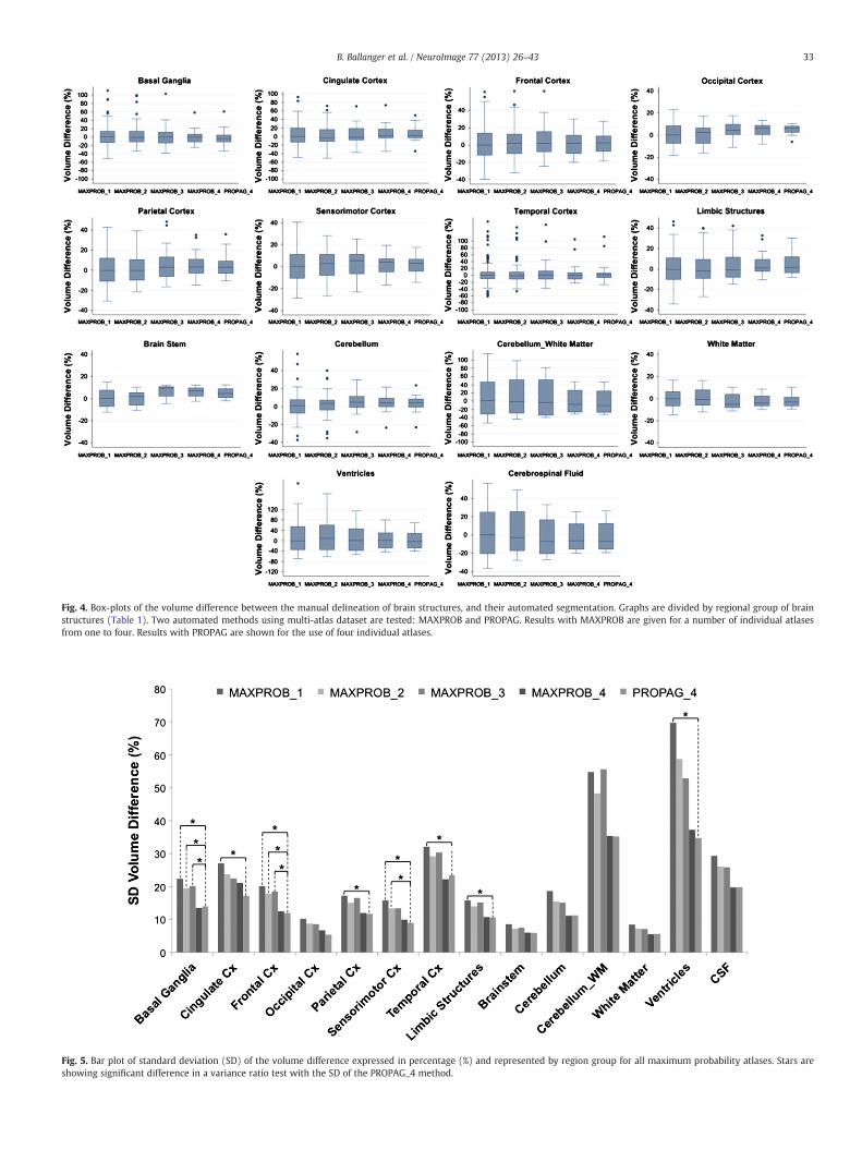
Fig. 4. Box-plots of the volume difference between the manual delineation of brain structures, and their automated segmentation. Graphs are divided by regional group of brainstructures (Table 1). Two automated methods using multi-atlas dataset are tested: MAXPROB and PROPAG. Results with MAXPROB are given for a number of individual atlasesfrom one to four. Results with PROPAG are shown for the use of four individual atlases.

Fig. 5. Bar plot of standard deviation (SD) of the volume difference expressed in percentage (%) and represented by region group for all maximum probability atlases. Stars areshowing significant difference in a variance ratio test with the SD of the PROPAG_4 method.

33B. Ballanger et al. / NeuroImage 77 (2013) 26–43

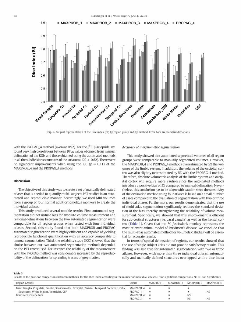
Fig. 6. Bar plot representation of the Dice index (SI) by region group and by method. Error bars are standard deviations.

34 B. Ballanger et al. / NeuroImage 77 (2013) 26–43

with the PROPAG_4 method (average 0.92). For the [11C]Raclopride, wefound very high correlations between BPND values obtained frommanualdelineation of the ROIs and those obtained using the automatedmethodsin all the subdivisions structures of the striatum (ICC > 0.82). Therewereno significant improvements when using the ICC (p = 0.11) of theMAXPROB_4 and the PROPAG_4 methods.

Discussion

The objective of this studywas to create a set ofmanually delineatedatlases that is needed to quantify multi-subjects PET studies in an auto-mated and reproducible manner. Accordingly, we used MRI volumesfrom a group of four normal adult cynomolgus monkeys to create theindividual atlases.

This study produced several notable results. First, automated seg-mentation did not induce bias for absolute volume measurement andregional delineations between the two automated segmentation werecomparable for all region groups when tested with four individualatlases. Second, this study found that both MAXPROB and PROPAGautomated segmentation were highly efficient and capable of yieldingreproducible functional quantification with an accuracy comparable tomanual segmentation. Third, the reliability study (ICC) showed that thechoice between our two automated segmentation methods dependedon the PET tracer used. For instance the reliability of the measurementwith the PROPAG method was considerably increased by the reproduc-ibility of the delineation for spreading tracers of grey matter.

Table 3Results of the post-hoc comparisons between methods, for the Dice index according to the

Region Groups

Basal Ganglia, Cingulate, Frontal, Sensorimotor, Occipital, Parietal, Temporal Cortices, LimStructures, White Matter, Ventricles, CSF

Brainstem, Cerebellum

Accuracy of morphometric segmentation

This study showed that automated segmented volumes of all regiongroups were comparable to manually segmented volumes. However,the MAXPROB_4 and PROPAG_4methods overestimated by 5% the vol-umes of the limbic system. In addition, the volume of the occipital cor-tex was also slightly overestimated by 5% with the PROPAG_4 method.Therefore, absolute volumetric analysis of the limbic system and occip-ital cortex will require more caution since the automated methodsintroduce a positive bias of 5% compared to manual delineation. Never-theless, this conclusion has to be takenwith caution since the sensitivityof the evaluation method using four atlases is based on a small numberof cases compared to the evaluation of segmentation with two or threeindividual atlases. Furthermore, our results demonstrated that the useof multi-atlas segmentation significantly reduces the standard devia-tion of the bias, thereby strengthening the reliability of volume mea-surement. Specifically, we showed that this improvement is efficientfor sub-cortical structures (i.e. basal ganglia) as well as the frontal cor-tex (Table 1). Given that the M. fascicularis monkey represents themost relevant animal model of Parkinson's disease, we conclude thatthemulti-atlas automatedmethod for volumetric studies will be essen-tial for accurate results.

In terms of spatial delineation of regions, our results showed thatthe use of single subject atlas did not provide satisfactory results. Thisfinding was also true for automated segmentation with two or threeatlases. However, with more than three individual atlases, automati-cally and manually defined structures overlapped with a dice index

number of individual atlases. (* for significant comparisons, NS = Non Significant).

versus MAXPROB_1 MAXPROB_2 MAXPROB_3 MAXPROB_4

bic MAXPROB_4 ✷ ✷ ✷

PROPAG_4 ✷ ✷ ✷ NSMAXPROB_4 ✷ ✷ NSPROPAG_4 ✷ ✷ NS NS

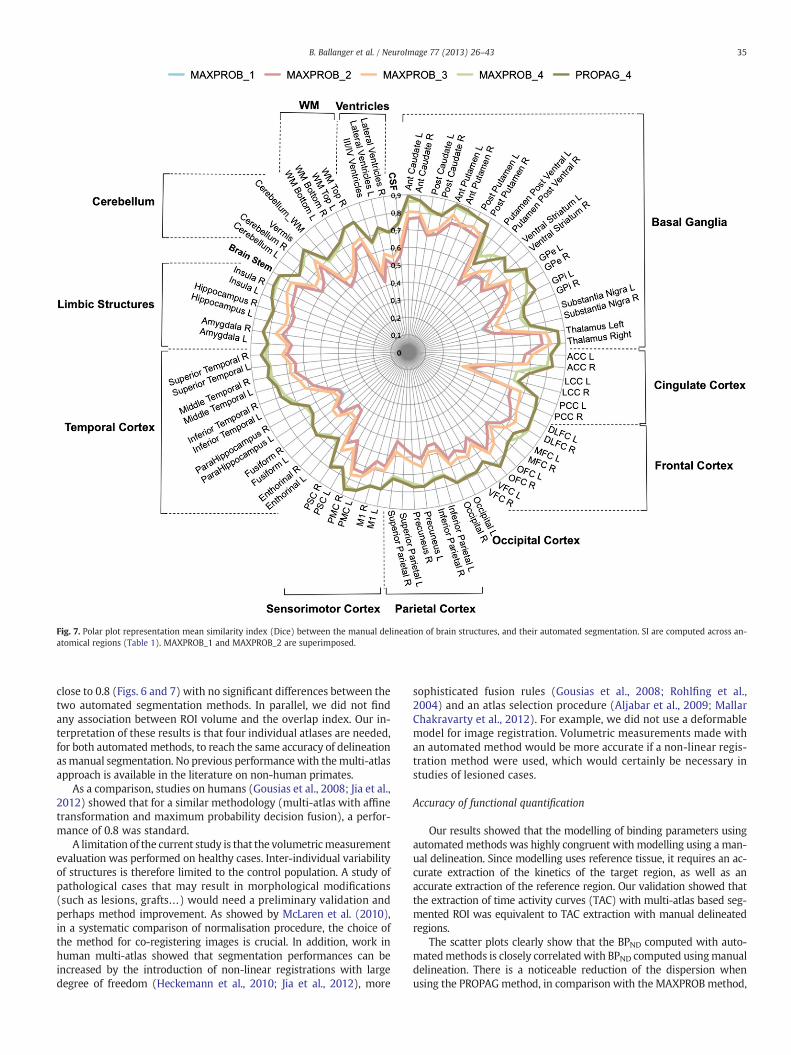
Fig. 7. Polar plot representation mean similarity index (Dice) between the manual delineation of brain structures, and their automated segmentation. SI are computed across an-atomical regions (Table 1). MAXPROB_1 and MAXPROB_2 are superimposed.

35B. Ballanger et al. / NeuroImage 77 (2013) 26–43

close to 0.8 (Figs. 6 and 7) with no significant differences between thetwo automated segmentation methods. In parallel, we did not findany association between ROI volume and the overlap index. Our in-terpretation of these results is that four individual atlases are needed,for both automated methods, to reach the same accuracy of delineationasmanual segmentation. No previous performancewith themulti-atlasapproach is available in the literature on non-human primates.

As a comparison, studies on humans (Gousias et al., 2008; Jia et al.,2012) showed that for a similar methodology (multi-atlas with affinetransformation and maximum probability decision fusion), a perfor-mance of 0.8 was standard.

A limitation of the current study is that the volumetricmeasurementevaluation was performed on healthy cases. Inter-individual variabilityof structures is therefore limited to the control population. A study ofpathological cases that may result in morphological modifications(such as lesions, grafts…) would need a preliminary validation andperhaps method improvement. As showed by McLaren et al. (2010),in a systematic comparison of normalisation procedure, the choice ofthe method for co-registering images is crucial. In addition, work inhuman multi-atlas showed that segmentation performances can beincreased by the introduction of non-linear registrations with largedegree of freedom (Heckemann et al., 2010; Jia et al., 2012), more

sophisticated fusion rules (Gousias et al., 2008; Rohlfing et al.,2004) and an atlas selection procedure (Aljabar et al., 2009; MallarChakravarty et al., 2012). For example, we did not use a deformablemodel for image registration. Volumetric measurements made withan automated method would be more accurate if a non-linear regis-tration method were used, which would certainly be necessary instudies of lesioned cases.

Accuracy of functional quantification

Our results showed that the modelling of binding parameters usingautomated methods was highly congruent with modelling using a man-ual delineation. Since modelling uses reference tissue, it requires an ac-curate extraction of the kinetics of the target region, as well as anaccurate extraction of the reference region. Our validation showed thatthe extraction of time activity curves (TAC) with multi-atlas based seg-mented ROI was equivalent to TAC extraction with manual delineatedregions.

The scatter plots clearly show that the BPND computed with auto-matedmethods is closely correlated with BPND computed usingmanualdelineation. There is a noticeable reduction of the dispersion whenusing the PROPAGmethod, in comparison with the MAXPROBmethod,

Fig. 8. Regression graphs of data from [11C]DASB (N = 11), [18F]MPPF (N = 10), and [11C]Raclopride (N = 13) studies obtained from individual ROIs and from ROIs derived fromMAXPROB_4 atlas (left column) and the PROPAG_4 atlas (right column). Linear regression curve equation and coefficient of correlation are given pooling data from the fourindividuals.

36 B. Ballanger et al. / NeuroImage 77 (2013) 26–43

especially for tracers that bind the cortical structures. This is visible onthe [11C]DASB scatter plots and to a lesser extent for the [18 F]MPPF,which is a little more specific to the limbic system. Study of the [11C]Raclopride, a selective tracer of the basal ganglia D2/D3 receptors, didnot significantly benefit from the PROPAG method compared to theMAXPROB method. Nevertheless, none of the paired t-tests betweenautomated andmanual binding parameter extractions were significant.Altogether, these findings validate the use of multi-atlas segmentationfor regional binding parameter computation.

Reproducibility

In this studywe evaluated the reproducibility of the regional bindingparameter estimation. This included an evaluation of the variability(bias and coefficient of variation), which represents the experimentaland the biological errors of the measurement. Knowledge of measure-ment errors is essential to predict the statistical power of a designstudy, including the computation of the sample size needed to detecta significant variation between two groups or between two conditions

in the same group (Costes et al., 2007). This variability and standarderror highly depends on the methodology used for parameter estima-tion. Our study validates the use of automatedmethods that have the re-producibility of the manual method. Moreover, it shows that multi-atlasbased segmentation reduces the standard error. With the MAXPROB_4method, reproducibility was lower, ranging from 0.58 to 0.91, and withmore variability, ranging from 8.2 to 19.2. The PROPAG_4 method re-duced the spread of measurement. Indeed, the variability of the repro-ducibility was halved with this method, compared to the maximumprobabilitymethod. The secondparameter evaluated in the reproducibil-ity study was the interclass coefficient. This parameter evaluated if thevariability of a test –retest measurement was negligible with regard tointer-individual variability. A high ICC means that the test –retest repro-ducibility and the standard error of themeasurement are negligible com-pared to the biological natural variability of the phenomenon. In ourreproducibility study, we showed that an ICC over 0.6 with theMAXPROB method reached the level of .8 and even 0.97 with thePROPAG method. These latest results, which are close to the maxi-mal value of 1, definitively validate the fact that automated methods

Table 4Non-displaceable binding potentials (BPND) computed with manual, maximum probability (MAXPROB_4) or propagated (PROPAG_4) atlases for the [18 F]MPPF, and for the [11C]Raclopride studies, in “control” conditions. Bias and SD Bias give the bias and the standard deviation of the bias of the BPND computed with the automated extraction versus themanual extraction. Intra-class correlation coefficient (ICC) gives the reproducibility of the BPND between manual and automated methods of extraction. Grey cells indicate the valueswhere the PROPAG_4 method is significantly better that the MAXPROB_4 method.

Manual Maximum probability atlas (MAXPROB_4) Propagated atlas (PROPAG_4)

Ligand

[18F]MPPF

[11C]Raclo

Region

Amygdala

Hippocampus

Enthorinal cortex

Anterior cingulate cortex

Frontal cortex

Occipital cortex

Parietal cortex

Posterior cingulate cortex

Temporal cortex

Whole striatum

Anterior caudate nucleus

Posterior caudate nucleus

Anterior putamen

Posterior putamen

Ventral posterior putamen

Ventral striatum

BPND

(mean ± SD)

1.23 ± 0.25

1.48 ± 0.34

1.12 ± 0.09

1.60 ± 0.36

1.21 ± 0.32

0.41 ± 0.11

1.09 ± 0.25

1.33 ± 0.19

0.81 ± 0.23

2.85 ± 0.88

3.03 ± 0.78

2.86 ± 0.52

3.21 ± 0.46

3.81 ± 0.22

2.31 ± 1.10

1.90 ± 0.45

BPND

(mean ± SD)

1.22 ± 0.20

1.47 ± 0.36

1.15 ± 0.11

1.65 ± 0.29

1.22 ± 0.28

0.39 ± 0.06

1.08 ± 0.20

1.34 ± 0.08

0.79 ± 0.23

2.88 ± 0.94

3.03 ± 0.85

2.89 ± 0.76

3.23 ± 0.56

3.87 ± 0.33

2.27 ± 1.07

1.96 ± 0.58

Bias (%)

1.3

-0.4

2.9

5.8

1.9

-0.2

0.7

2.2

-1.5

0.5

-0.7

-0.3

0.5

1.6

-0.7

2.8

SD Bias (%)

16.5

14.0

8.2

16.6

9.7

19.2

12.7

10.2

12.2

10.4

4.2

13.8

6.5

6.3

16.4

11.8

ICC

0.75

0.74

0.91

0.69

0.88

0.58

0.77

0.81

0.87

0.95

0.99

0.86

0.96

0.98

0.93

0.83

BPND

(mean ± SD)

1.21 ± 0.24

1.43 ± 0.35

1.14 ± 0.10

1.65 ± 0.30

1.19 ± 0.31

0.40 ± 0.09

1.09 ± 0.23

1.33 ± 0.14

0.82 ± 0.23

2.85 ± 0.92

3.04 ± 0.88

2.78 ± 0.67

3.20 ± 0.44

3.83 ± 0.32

2.26 ± 1.10

1.96 ± 0.57

Bias (%)

-0.9

-3.0

1.9

4.5

-1.1

-0.3

1.2

1.0

1.1

-0.5

-0.8

-3.5

-0.1

0.7

-2.3

2.8

SD Bias(%)

8.4

9.0

5.8

8.2

6.7

9.3

7.3

4.8

6.4

9.2

8.4

11.9

4.3

6.5

12.2

10.1

ICC

0.92

0.88

0.95

0.91

0.94

0.88

0.92

0.96

0.97

0.96

0.97

0.88

0.98

0.98

0.96

0.87

37B. Ballanger et al. / NeuroImage 77 (2013) 26–43

provide a reliable way of evaluating regional PET binding parameters.These findings are particularly evident with PET tracers that bind to thecortex such as, here, the [18 F]MPPF. In fact, for tracers of specific sub-cortical structures, such as the [11C]Raclopride, the reliability of the func-tional quantification with the MAXPROB_4 method was high (around10%) and this result was not improved by the PROPAG_4 method.

Rationale for the multi-subject atlas method

In the present study, we introduced, created and validated a multi-atlas based automated segmentation method. With this approach, theatlas does not rely on the anatomy of a single subject, but instead de-pends on nonlinear normalisation of numerous cynomolgus monkeybrains mapped to an average MRI template image that is faithful tothe location of anatomical structures. Combining information frommul-tiple sources can compensate for the potential bias introduced by usinga single atlas. The multi-atlas approach yields greater accuracy (Collinsand Pruessner, 2010). In this study, each atlas consisted of 42 anatomicalROIs, which, together, covered the whole brain, brainstem and cerebel-lum aswell as ventricles, whitematter and cerebrospinal fluid. Althoughthe delineation of the ROIs was operator-dependent and may be subjec-tive, a detailed delineation protocol along the three orthogonal planeswas used to define consistent and precise delineations (see Appendix A).

Both morphometric and functional evaluations showed that per-formances were increased with a multi-subject atlas, and specifically,that maximal performances were reached with four individual atlases.

Use of the MRI template and the maximum probability atlas in a referencespace

We demonstrated the usefulness of aM. fascicularis brain templateand its associated ROIs atlas to spatially normalise and quantify PETstudies in a fully automated way. Indeed, our work allows the spatialnormalisation of a dataset in the same reference space and thus al-lows voxel-by-voxel statistical analysis to be performed, as is widelydone in human PET analysis, using, for instance, statistical parametricmapping (SPM) (Friston et al., 1994). Indeed, our ROIs atlas can beused to align many individual monkeys to carry out voxel-based anal-yses of multi-subject parametric images (Ashburner et al., 1998;Friston et al., 1999). The maximum probability atlas in the referencespace may also be used for anatomical localization of a cluster of

interest issuing from an SPM, for functional connectivity analysis ofinter-regional activations, and for voxel-basedmorphometry analyses

Finally, the multi atlas-segmentation method will allow functionalquantification to give an accurate regional value and/or kinetic extrac-tion, which would take into account the individual neuroanatomicalvariability. In addition, accurate segmentation of the brain and the sur-rounding structures is appropriate for processing partial volume effectcorrection, for example with the GTM method (Rousset et al., 2008).Implementing automated segmentation for morphometric volumetricanalysis might be further extended to pathological cases after introduc-tion of non-linear registration methods, as has already been done inhumans (Heckemann et al., 2011; Keihaninejad et al., 2012).

In conclusion, we obtained and validated a brain M. fascicularis tem-plate and its reference atlas for use as targets of automatic, voxel-basedimage registration methods. These new ROIs atlas address unmet needsfor neuroimaging research in non-human primates. To our knowledge,this is thefirst approach that incorporates a largenumber of ROIs in an au-tomatic anatomical segmentationmethod applicable to theM. fascicularispopulation. We demonstrated the adequacy and practical usefulness ofthe constructed template and the corresponding atlas. We believe theavailability of these references will be helpful for future intra- and inter-individual voxel-based, longitudinal and multi-tracer analyses, and willfacilitate analysis of neuroimaging studies inM. fascicularis.

By considering themulti-atlas set, the preliminary definition of an im-aging protocol will have to consider the degree of accuracy of extractedparameters. Functional imaging studies that do not assess morphologicvariation will not require an individual MRI for a tracer specific to a sub-cortical structure. Indeed, we showed that this economic choice wouldnot affect the performance or the statistical power of the study. However,for a tracer known to bind a cortical structure, an accurate procedure forregional binding parameter extraction will require an individual MRI. Bykeeping this inmind, themethodological approach of the two automatedtechniques differed in one major aspect: automated segmentation withthepropagated atlas needs anMRI of the subject,whereas automated seg-mentation with the maximum probability atlas does not.

Acknowledgements

We gratefully thank the radiochemistry team in the CERMEP,Frédéric Bonnefoi, Marion Malleval-Alvarez, the cyclotron operator,Christian Tourvielle, and the MRI staff, Jean-Christophe Comte and

Labels 9 and 10Internal Pallidum (right, left).

Orientation of slices CoronalAnterior border Start on first slice on which the frontal horn of the lateral

38 B. Ballanger et al. / NeuroImage 77 (2013) 26–43

Fabienne Vey. We thank Vincent Leviel for providing MRI scans. Valu-able help was provided by Alexander Hammers and Rolf Heckemann.This work was supported by the French National Agency of Research(grant number ANR-09-MNPS-018).

ventricle and the third ventricles are joined.Posterior border Last slice where visibleMedial border WMLateral border External pallidumSuperior border Internal capsule (Line drawn by the superior borders of

posterior putamen and external pallidum)Inferior border WM (Horizontal line drawn by inferior borders of posterior

putamen and external pallidum)Number of slices ~8

Appendix A. Delineation protocol

Each region is defined in terms of its defining boundaries in eachdimension according to Martin and Bowden's nomenclature (1996).When this is insufficient, footnotes are used.

Labels 1 and 2Anterior Caudate Nucleus (right, left).

Orientation of slices CoronalAnterior border Start on first slice on which caudate nucleus is visible at the

lateral border of the lateral ventriclePosterior border Last slide on which the anterior commissure is completely

visualisedMedial border Lateral ventricleSuperior border WMLateral border WMInferior border Anterior → Posterior: WM, Ventral Striatum, WMNumber of slices ~15

Labels 3 and 4Anterior Putamen (right, left).

Orientation of slices CoronalAnterior border Most anterior slice where putamen is seenPosterior border Last slide on which the anterior commissure is

completely visualisedMedial border Anterior → Posterior: Internal capsule/Ventral

Striatum, External pallidumLateral border WM (External capsule)Superior border WMInferior border WMNumber of slices ~12

Labels 5 and 6Ventral Striatum (right, left).

Include inferior part of the anterior striatum, accumbens nucleus and substantia innominata.Orientation of slices Coronal; start posteriorlyAnterior border Last slice where ventral striatum can be clearly

differentiated from the anterior caudate nucleus(e.g. inferior part of the anterior caudate visible)

Posterior border First slice after the anterior commissure is fully visibleMedial border Lateral ventricle, WMLateral border WMSuperior border Anterior striatum (Ventral striatum is always inferior

to lateral ventricle)Inferior border Anterior → Posterior: WM, Anterior CommissureNumber of slices ~15

Labels 7 and 8External Pallidum (right, left).

Orientation of slices CoronalAnterior border First slice on which the anterior commissure is completely

visualisedPosterior border Last slice where visibleMedial border Anterior → Posterior: WM, Internal pallidum, WMLateral border PutamenSuperior border Internal capsuleInferior border Anterior → Posterior: WM, Ventral posterior putamen, WMNumber of slices ~13

Labels 11 and 12Posterior Caudate Nucleus (right, left).

Orientation of slices CoronalAnterior border Anterior caudate nucleusPosterior border Last slice where visibleMedial border Lateral ventricleLateral border WMSuperior border WMInferior border Anterior → Posterior: WM, Thalamus, WMNumber of slices ~21

Labels 13 and 14Posterior Putamen (right, left).

Orientation of slices CoronalAnterior border Anterior putamenPosterior border Last slice where visibleMedial border Anterior → Posterior: External pallidum, WMLateral border WM (external capsule)Superior border WMInferior border Anterior → Posterior: WM, ventral posterior putamen, WMNumber of slices ~19

Labels 15 and 16Ventral Posterior Putamen (right, left).

Orientation of slices CoronalAnterior border Start on first slice on which the third ventricle is discontinuedPosterior border Last slice where visibleMedial border WMLateral border WMSuperior border Inferior borders of posterior putamen and external pallidumInferior border WMNumber of slices ~12

Caution: Use sagittal orientation for help with superior, lateral and inferior borders.

Labels 17 and 18Substantia Nigra (right, left).

Orientation of slices CoronalAnterior border Level of the mamillary bodiesPosterior border Last slide where visibleMedial border Brain StemLateral border Brain StemSuperior border Brain StemInferior border Brain StemNumber of slices ~10

Caution: Use transverse orientation initially to aid the delineation of the structurewhere the nigra is clearly visible in its entire anteroposterior extent.

Labels 21 and 22Hippocampus (right, left).

Orientation of slices CoronalAnterior border Start on first slice where the internal pallidum begins

(as previously defined, see Labels 9 and 10).Posterior border Most posterior slice where the body and the temporal

horn of lateral ventricle fuse, before the occipital hornof lateral ventricle begins

Medial border Anterior → Posterior: Enthorinal area, CSF,Parahippocampal gyrus; WM

Lateral border Anterior → Posterior: WM, Lateral VentricleSuperior border Anterior → Posterior: Amygdala, WM, and CSFInferior border Anterior → Posterior: Enthorinal area, WMNumber of slices ~27

Labels 23 and 24Amygdala (right, left).

Include prepyriform and periamygdaloid areas, amygdala, basolateral nuclear group,basal and cortical amygdaloid nuclei.Orientation of slices CoronalAnterior border Start on first slide on which the rhinal sulcus is visiblePosterior border Most posterior slice before thalamus appears

(as previously defined, see Labels 19 and 20)Medial border CSFLateral border Anterior → Posterior: Superior temporal gyrus, WMSuperior border Anterior → Posterior: CSF, WMInferior border Anterior → Posterior: CSF, Middle temporal gyrus,

Enthorinal area, HippocampusNumber of slices ~14

Labels 27 and 28Insula (right, left).

Orientation of slices CoronalAnterior border First slice on which insular sulcus is visualisedPosterior border Last slice on which insular sulcus is visualisedMedial border WM (Lateral edge of the extreme or external capsule)Lateral border CSF within lateral sulcusSuperior border Insular sulcusInferior border Insular sulcusNumber of slices ~26

Caution: Start by estimating anterior–posterior and superior–inferior extent with sagittalslices when the insular sulcus is completely visible.

Labels 19 and 20Thalamus (right, left).

Orientation of slices CoronalAnterior border Start on first slice on which the third ventricle is

discontinuedPosterior border Last slice where visibleMedial border Midline/Third ventricleLateral border WMSuperior border WM then more posteriorly draw an horizontal line

following the inferior borders of lateral ventricleInferior border Anterior → Posterior: WM, Brain Stem, WMNumber of slices ~15

Caution: The use of the mid-sagittal slices facilitated more accurate determination of thedifferent borders. In addition use the transverse orientation for help with lateral borders.

Labels 29 and 30Cerebellum (right, left).

Orientation of slices SagittalAnterior border First slice on which the cerebellar peduncle joins the brainstemPosterior border CSFMedial border Vermis (see structure 72)Lateral border CSFSuperior border CSFInferior border CSFNumber of slices ~34

Labels 31 and 32Orbitofrontal Cortex (right, left).

Include gyrus rectus; medial, lateral, and fronto-orbital gyri.Orientation of slices CoronalAnterior border CSFPosterior border End one slice before insula appears (as previously

defined, see Labels 27 and 28)Medial border MidlineLateral border Anterior → Posterior: CSF, Precentral Gyrus, WMSuperior/lateral border Anterior → Posterior: Inferior frontal gyrus, WM,

Extreme capsuleSuperior/medial border Anterior → Posterior: Superior frontal gyrus, Anterior

cingulate gyrus/Rostral sulcusInferior border CSFNumber of slices ~36

Labels 33 and 34Anterior Cingulate Cortex (right, left).

Orientation of slices Sagittal then coronalSagittal cutsAnterior border Cingulate sulcusPosterior border Draw a vertical line from corpus callosum to cingulate

sulcus at the mid-point of the greatest extension of thecorpus callosum on most medial slice; corpus callosuminferiorly

Medial border MidlineLateral border Last slice on which cingulate sulcus is visible in its full

length (then change to coronal cuts)Superior border Cingulate sulcus

Coronal cutsAnterior border As previously defined on sagittal cutsPosterior border As previously defined on sagittal cutsMedial border As previously defined on sagittal cutsLateral border WMSuperior border As previously defined on sagittal cutsInferior border Anterior → Posterior: Gyrus rectus, Rostral sulcus,

Callosal sulcusNumber of slices ~38

Labels 35 and 36Limbic Cingulate Cortex (right, left).

Orientation of slices CoronalAnterior border First slice when the genu of corpus callosum appearsPosterior border End when insular sulcus is visibleMedial border MidlineLateral border WMSuperior border Corpus CallosumInferior border Anterior → Posterior: Rostral sulcus, Gyrus rectusNumber of slices ~6

Labels 37 and 38Posterior Cingulate Cortex (right, left).

Orientation of slices CoronalAnterior border Anterior cingulate cortexPosterior border Subparietal sulcus (mid-sagittal orientation)Medial border MidlineLateral border WMSuperior border Anterior → Posterior: Cingulate sulcus, Precuneus,

Subparietal sulcusInferior border Anterior → Posterior: Callosal sulcus, CuneusNumber of slices ~34

39B. Ballanger et al. / NeuroImage 77 (2013) 26–43

Labels 39 and 40Dorsolateral frontal Cortex (right, left).

Include superior and middle frontal gyri.Orientation of slices CoronalAnterior border CSFPosterior border Last slice = last slice where the principal sulcus

is visibleMedial border Anterior → Posterior: Superior frontal gyrus

(medial part), Superior ramus of arcuate sulcusLateral border CSFSuperior border CSFInferior border Principal sulcusNumber of slices ~32

Labels 41 and 42Parahippocampal Gyrus (right, left).

Orientation of slices CoronalAnterior border Start on first slice on which rhinal sulcus is no longer

visiblePosterior border Posterior border of the hippocampus as previously

defined (that slice included, see Labels 21 and 22)Medial border CSFLateral/Superior border Anterior → Posterior: Hippocampus, WMLateral/Inferior border Fusiform gyrusSuperior border Anterior → Posterior: Hippocampus, CSFInferior border CSFNumber of slices ~20

Labels 43 and 44Superior Temporal Cortex (right, left).

Orientation of slices CoronalAnterior border CSFPosterior border End when the lateral sulcus is no longer visibleMedial Border Anterior → Posterior: CSF, Rhinal Sulcus, WM, Insular

sulcus, WMLateral border CSFSuperior border Anterior → Posterior: CSF, Lateral sulcusInferior border Anterior → Posterior: CSF, Superior temporal sulcusNumber of slices ~56

Labels 45 and 46Medial Temporal Cortex (right, left).

Orientation of slices CoronalAnterior border Locate the first slice on which the superior temporal

as well as the rhinal sulci are visible. Then draw horizontalline between both.

Posterior border End one slide before inferior occipital sulcus appearsMedial Border Anterior → Posterior: CSF, Inferior temporal gyrus, Anterior

middle temporal sulcus, WMLateral border CSFSuperior border Superior temporal sulcusInferior border Anterior → Posterior: CSF, Inferior temporal gyrusNumber of slices ~45

Labels 47 and 48Inferior Temporal Cortex (right, left).

Orientation of slices CoronalAnterior border Start on the slide where insula appears (as previously

defined, see Labels 27 and 28)Posterior border Posterior border of the medial temporal cortex

(as previously defined, see Labels 45 and 46)Medial border Anterior → Posterior: CSF, rhinal sulcus, Fusiform gyrus,

Occipito-temporal sulcusLateral border Anterior → Posterior: WM, Middle temporal gyrus,

Anterior middle temporal sulcus, Middle temporal gyrusSuperior border Anterior → Posterior: Rhinal sulcus, middle temporal

sulcus, WMInferior border Anterior → Posterior: Middle temporal gyrus, CSFNumber of slices ~43

Labels 49 and 50Occipital Cortex (right, left).

Include inferior occipital gyrus, lingual gyrus, cuneus and occipital gyrusOrientation of slices First sagittal, then transverseSagittal cuts (start medially)

Anterior border Parieto-occipital sulcusPosterior border CSFMedial border MidlineLateral border Last slice on which parieto-occipital sulcus is visible

in its full length (then change to transverse cuts)Superior border Parieto-occipital sulcus/CSFInferior border CSF (Cerebellar tentorium)

Transverse cutsAnterior border Straight line between medial end of anterior

occipital sulcus, and lateral end of parieto-occipitalsulcus

Posterior border As previously defined on sagittal cutsMedial border As previously defined on sagittal cutsLateral border CSFSuperior border Anterior occipital sulcusInferior border As previously defined on sagittal cuts

Number of slices ~39 (coronal)

Labels 51 and 52Superior Parietal Cortex.

Orientation of slices CoronalAnterior border Start when the putamen posterior ventral is no longer

visible (as previously defined, see Labels 15 and 16)Posterior border Last slide where the intraparietal sulcus is visible; CSFMedial border Anterior → Posterior: WM, Midline, Cingulate sulcus,

PrecuneusLateral border Anterior → Posterior: CSF, Intraparietal sulcusSuperior border Anterior → Posterior: Postcentral gyrus, Superior

postcentral sulcus, CSFInferior border Anterior → Posterior: Intraparietal sulcus, Cingulate

sulcus, Simian fossa, WMNumber of slices ~34

Caution: The use of the sagittal and transverse slices facilitates more accurate determinationof the different borders on slices where the intraparietal sulcus is clearly visible.

Labels 53 and 54Inferior Parietal Cortex (right, left).

Include the angular and supramarginal gyri.Orientation of slices CoronalSupramarginal gyrus

Anterior border Start on first slide on which intraparietal sulcus isclearly visible

Medial border WMLateral border CSFSuperior border Intraparietal sulcusInferior border Lateral sulcus

Angular gyrusAnterior border Start on first slide on which inferior occipital sulcus

is visibleMedial border WMLateral border CSFSuperior border Superior temporal sulcusInferior border Inferior occipital sulcus

Then when the lateral sulcus is no longer visible the supramarginal and angulargyri fuse.

Posterior border End when intraparietal and lunate sulci disappear.Medial border Anterior → Posterior: WM, Intraparietal sulcusLateral border CSFSuperior border Anterior → Posterior: Intraparietal sulcus, CSFInferior border Anterior → Posterior: Inferior occipital sulcus,

lunate sulcus, simian fossaNumber of slices ~35

40 B. Ballanger et al. / NeuroImage 77 (2013) 26–43

Labels 55 and 56Precuneus (right, left).

Orientation of slices Coronal then transverseCoronal cuts

Anterior border First slide = Last slide where the splenium ofcorpus callosum is visible

Posterior border Last slide where the intraparietal sulcus is visibleTransverse cuts

Medial border MidlineLateral border WMSup/Ant. border Cingulate sulcusSup/Post. border Superior→ Inferior: Superior parietal cortex, CSF,

Occipital CortexInf./Ant. border Anterior parieto-occipital sulcusInf./Post. border Parieto-occipital sulcusNumber of slices ~24 (coronal)

Labels 57 and 58Premotor Cortex (right, left).

Include superior frontal gyrus (dorsal part) and precentral gyrus (ventral part)Orientation of slices CoronalDorsal premotor cortexAnterior border Start on first slide on which genu of corpus callosum

appearsMedial border MidlineSuperior border CSFInf./Med. border Cingulate sulcusInf./Lat. Border Superior ramus of arcuate sulcus

Ventral premotor cortexAnterior border Start on first slide on which inferior ramus of arcuate

sulcus is visibleMedial border Fronto-orbital gyrusLateral border CSFSuperior border Inferior ramus of arcuate sulcusInferior border Anterior → Posterior: CSF, Lateral sulcus

Then dorsal and ventral premotor parts join when the principal sulcus is no longervisiblePosterior border End one slice before the central sulcus appearsMedial border MidlineLateral border CSFSuperior border CSFInf./Med. border Cingulate sulcusInf./Lat. Border Anterior → Posterior: Insular sulcus, Anterior

subcentral sulcus, Superior arcuate sulcusNumber of slices ~27

Labels 59 and 60Primary Motor Cortex (right, left).

Orientation of slices Transverse then coronalTransverse cuts

Anterior border Posterior border of the premotor cortexPosterior border Central sulcus

Coronal cutsMedial border Anterior → Posterior: WM, MidlineLateral border CSFSuperior border Anterior → Posterior: Superior arcuate sulcus, CSFInf./Lat. border Central sulcusInf./Med. border Cingulate sulcus

Number of slices ~25 (coronal)

Caution: Use transverse orientation to help delineate the posterior border along the centralsulcus.

Labels 61 and 62Primary Sensory Cortex (right, left).

Orientation of slices CoronalStart anteriorly with the lateral part of the structure

Anterior border Same level that putamen posterior (as previouslydefined, see Labels 13 and 14)

Medial border Anterior → Posterior: Insular sulcus, Central sulcusLateral border CSFSuperior border Anterior → Posterior: Anterior subcentral sulcus,

Central sulcus, CSFInferior border Anterior → Posterior: Lateral sulcus, Intraparietal

sulcus, Superior parietal cortexWhen the intraparietal sulcus begins start to draw the medial part of the structure

Medial border MidlineLateral border WMSuperior border Primary motor cortexInferior border Cingulate sulcus

Then when central sulcus is no longer visible the lateral and medial parts of theprimary sensory cortex fusePosterior border End when the superior postcentral sulcus is no

longer visibleNumber of slices ~33

Caution: Use transverse orientation to help delineate the anterior border along thecentral sulcus.

Labels 63 and 64Ventral frontal Cortex (right, left).

Include Inferior and middle frontal gyri.Orientation of slices CoronalAnterior border CSFPosterior border End when the principal sulcus is no longer visibleMedial border WMLateral border CSFSuperior border Principal sulcus/CSFInferior border Anterior → Posterior: Fronto-Orbital gyrus/CSF,

Inferior ramus of arcuate sulcusNumber of slices ~32

Labels 65 and 66Fusiform Gyrus (right, left).

Orientation of slices CoronalAnterior border Start on first slice on which parahippocampal gryus is

visualised (as previously defined, see Labels 41 and 42)Posterior border Last slide where occipito-temporal sulcus is visibleMedial border Anterior → Posterior: Parahippocampal gyrus, Collateral

sulcusLateral border Anterior → Posterior: Inferior temporal gyrus,

Occipito-temporal sulcusSuperior border WMInferior border CSFNumber of slices ~45

Labels 67 and 68Enthorinal Cortex (right, left).

Orientation of slices CoronalAnterior border Start on first slice on which insula begins (as previously

defined, see Labels 27 and 28)Posterior border Anterior border of parahippocampal and fusiform gyri as

previously defined (see Labels 41 and 42 and 65 and 66respectively)

Medial border CSFLateral border Anterior → Posterior: WM, HippocampusSuperior border Anterior → Posterior: Amygdala, HippocampusInferior border Anterior → Posterior: Inferior temporal cortex, CSFNumber of slices ~15

41B. Ballanger et al. / NeuroImage 77 (2013) 26–43

Labels 69 and 70Medial frontal Cortex (right, left).

Orientation of slices CoronalAnterior border CSFPosterior border End one slide before the genu of corpus callosum is visualisedMedial border MidlineLateral border Anterior → Posterior: Dorsolateral frontal cortex, WMSuperior border CSFInferior border Anterior → Posterior: Gyrus rectus, Cingulate sulcusNumber of slices ~23

Label 72Vermis.

Orientation of slices CoronalAnterior border Begin at the cerebellum mid-sagittal slicePosterior border CerebellumMedial border MidlineLateral border CSFSuperior border CSFInferior border CSFNumber of slices ~33

Labels 80 and 81White Matter, top part (right, left).

Include corpus callosum, internal capsule, external capsule, extreme capsuleOrientation of slices TransverseInclude all remaining area above the virtual horizontal line drawnby posterior borders of thalamus, posterior putamen and insula.

Labels 82 and 83White Matter, bottom part (right, left).

The remaining area after drawing the top part

Label 84Brain Stem.

Orientation of slices SagittalAnterior border CSFPosterior border CSFMedial border No medial border, spans the midlineLateral border CSFSuperior border Cut from basal ganglia as soon as pedunculus cerebri

enters them using a tangential line following thecontours of the basal ganglia.

Inferior border Inferior border of the cerebellumNumber of slices ~32

Caution: Start at the mid-sagittal slice and work medial to lateral.

Labels 85 and 86Lateral Ventricles (right, left).

Include frontal, body and occipital horns of the lateral ventricles.Orientation of slices CoronalAnterior border Start on first slice on which frontal horn is visiblePosterior border Last slide where the occipital horn of lateral ventricle

is visibleMedial border Anterior → Posterior: WM, Midline/Third ventricleLateral border Anterior → Posterior: Anterior caudate nucleus,

Ventral striatum, Posterior caudate nucleusSuperior border WMInferior border Anterior → Posterior: WM, Ventral striatum, WM (Anterior

commissure), Third ventricle/WM, Thalamus, WMNumber of slices ~55

Label 87Third and Fourth Ventricles.

Orientation of slices CoronalThird ventricle

Anterior border Lamina terminalis (CSF)Posterior border Pineal glandMedial border None (midline structures)Lateral border Anterior → Posterior: WM, Thalamus, WMSuperior border Fornix (WM)Inferior border Anterior → Posterior: Optic chiasma, WM

Fourth ventricleAnterior border First slice on which the fourth ventricle is seen

between the brain stem and cerebellumPosterior border Last slide where visibleMedial border None (midline structures)Lateral border Brain StemSuperior border Brain StemInferior border Brain Stem

Number of slices ~38

Label 88Cerebellum White Matter.

The remaining area after drawing the cerebellum (grey matter) and the vermisNumber of slices ~23 (coronal)

Label 89Cerebrospinal Fluid.

The remaining area after drawing all the structures defined above

42 B. Ballanger et al. / NeuroImage 77 (2013) 26–43

References

Aljabar, P., Heckemann, R.A., Hammers, A., Hajnal, J.V., Rueckert, D., 2009. Multi-atlas basedsegmentation of brain images: atlas selection and its effect on accuracy. NeuroImage46, 726–738.

Ashburner, J., Hutton, C., Frackowiak, R., Johnsrude, I., Price, C., Friston, K., 1998. Identifyingglobal anatomical differences: deformation-based morphometry. Hum. Brain Mapp. 6,348–357.

Black, K.J., Gado, M.H., Videen, T.O., Perlmutter, J.S., 1997. Baboon Basal Ganglia StereotaxyUsing Internal MRI Landmarks: Validation and Application to PET Imaging. J. Comput.Assist. Tomogr. 21, 881.

Black, K.J., Koller, J.M., Snyder, A.Z., Perlmutter, J.S., 2001a. Template images for nonhumanprimate neuroimaging: 2. Macaque. NeuroImage 14, 744–748.

Black, K.J., Snyder, A.Z., Koller, J.M., Gado, M.H., Perlmutter, J.S., 2001b. Template imagesfor nonhuman primate neuroimaging: 1. Baboon. NeuroImage 14, 736–743.

Blesa, J., Pifl, C., Sánchez-González, M.A., Juri, C., García-Cabezas, M.A., Adánez, R., Iglesias, E.,Collantes, M., Peñuelas, I., Sánchez-Hernández, J.J., Rodriguez-Oroz, M.C., Avendaño, C.,Hornykiewicz, O., Cavada, C., Obeso, J.A., 2012. The nigrostriatal system in thepresymptomatic and symptomatic stages in theMPTPmonkeymodel: A PET, histolog-ical and biochemical study. Neurobiol. Dis. 48, 79–91.

Brix, G., Zaers, J., Adam, L.E., Bellemann, M.E., Ostertag, H., Trojan, H., Haberkorn, U., Doll,J., Oberdorfer, F., Lorenz, W.J., 1997. Performance evaluation of a whole-body PETscanner using the NEMA protocol. National Electrical Manufacturers Association.J. Nucl. Med. 38, 1614–1623.

Brown, C.A., Campbell, M.C., Karimi, M., Tabbal, S.D., Loftin, S.K., Tian, L.L., Moerlein,S.M., Perlmutter, J.S., 2012. Dopamine pathway loss in nucleus accumbens and ven-tral tegmental area predicts apathetic behavior in MPTP-lesioned monkeys. Exp.Neurol. 236, 190–197.

Collantes, M., Prieto, E., Peñuelas, I., Blesa, J., Juri, C., Martí-Climent, J.M., Quincoces, G.,Arbizu, J., Riverol, M., Zubieta, J.L., Rodriguez-Oroz, M.C., Luquin, M.R., Richter, J.A.,Obeso, J.A., 2009. New MRI, 18 F-DOPA and 11C-(+)-alpha-dihydrotetrabenazinetemplates for Macaca fascicularis neuroimaging: advantages to improve PET quan-tification. NeuroImage 47, 533–539.

Collins, D.L., Pruessner, J.C., 2010. Towards accurate, automatic segmentation of thehippocampus and amygdala from MRI by augmenting ANIMAL with a template li-brary and label fusion. NeuroImage 52, 1355–1366.

Collins, D.L., Neelin, P., Peters, T.M., Evans, A.C., 1994. Automatic 3D intersubject registrationof MR volumetric data in standardized Talairach space. J. Comput. Assist. Tomogr. 18,192–205.

Costes, N., Zimmer, L., Reilhac, A., Lavenne, F., Ryvlin, P., Le Bars, D., 2007. Test–retest re-producibility of 18 F-MPPF PET in healthy humans: a reliability study. J. Nucl. Med.48, 1279–1288.

Fox, P.T., Perlmutter, J.S., Raichle, M.E., 1985. A stereotactic method of anatomical locali-zation for positron emission tomography. J. Comput. Assist. Tomogr. 9, 141–153.

Frey, S., Pandya, D.N., Chakravarty, M.M., Bailey, L., Petrides, M., Collins, D.L., 2011. AnMRIbased average macaque monkey stereotaxic atlas and space (MNI monkey space).NeuroImage 55, 1435–1442.

43B. Ballanger et al. / NeuroImage 77 (2013) 26–43

Friston, K.J., Holmes, A.P., Worsley, K.J., Poline, J.P., Frith, C.D., Frackowiak, R.S.J., 1994.Statistical parametric maps in functional imaging: A general linear approach. Hum.Brain Mapp. 2, 189–210.

Friston, K.J., Ashburner, J., Frith, C.D., Poline, J.B., Heather, J.D., Frackowiak, R.S.J., 1995.Spatial registration and normalization of images. Hum. Brain Mapp. 3, 165–189.

Friston, K.J., Holmes, A.P., Price, C.J., Buchel, C., Worsley, K.J., 1999. Multisubject fMRIstudies and conjunction analyses. NeuroImage 10, 385–396.

Gousias, I.S., Rueckert, D., Heckemann, R.A., Dyet, L.E., Boardman, J.P., Edwards, A.D.,Hammers, A., 2008. Automatic segmentation of brain MRIs of 2-year-olds into 83regions of interest. NeuroImage 40, 672–684.

Greer, P.J., Villemagne, V.L., Ruszkiewicz, J., Graves, A.K., Meltzer, C.C., Mathis, C.A.,Price, J.C., 2002. MR atlas of the baboon brain for functional neuroimaging. BrainRes. Bull. 58, 429–438.

Gunn, R.N., Laamerstma, A.A., Hume, S.P., Cunningham, V.J., 1997. Parametric imagingof ligand-receptor binding in PET using a simplified reference region. NeuroImage6, 279–287.

Hammers, A., Koepp, M.J., Free, S.L., Brett, M., Richardson, M.P., Labbé, C., Cunningham,V.J., Brooks, D.J., Duncan, J., 2002. Implementation and application of a brain tem-plate for multiple volumes of interest. Hum. Brain Mapp. 15, 165–174.

Hammers, A., Allom, R., Koepp, M.J., Free, S.L., Myers, R., Lemieux, L., Mitchell, T.N.,Brooks, D.J., Duncan, J.S., 2003. Three-dimensional maximum probability atlasof the human brain, with particular reference to the temporal lobe. Hum. BrainMapp. 19, 224–247.

Heckemann, R.A., Hajnal, J.V., Aljabar, P., Rueckert, D., Hammers, A., 2006. Automaticanatomical brainMRI segmentation combining label propagation and decision fusion.NeuroImage 33, 115–126.

Heckemann, R.A., Keihaninejad, S., Aljabar, P., Rueckert, D., Hajnal, J.V., Hammers, A.,Alzheimer's Disease Neuroimaging Initiative, 2010. Improving intersubject imageregistration using tissue-class information benefits robustness and accuracy of multi-atlas based anatomical segmentation. NeuroImage 51, 221–227.

Heckemann, R.A., Keihaninejad, S., Aljabar, P., Gray, K.R., Nielsen, C., Rueckert, D., Hajnal,J.V., Hammers, A., Alzheimer's Disease Neuroimaging Initiative, 2011. Automaticmorphometry in Alzheimer's disease and mild cognitive impairment. NeuroImage56, 2024–2037.

Hikishima, K., Quallo, M.M., Komaki, Y., Yamada, M., Kawai, K., Momoshima, S., Okano,H.J., Sasaki, E., Tamaoki, N., Lemon, R.N., Iriki, A., Okano, H., 2011. Population-averagedstandard template brain atlas for the common marmoset (Callithrix jacchus).NeuroImage 54, 2741–2749.

Jia, H., Yap, P.-T., Shen, D., 2012. Iterative multi-atlas-based multi-image segmentationwith tree-based registration. NeuroImage 59, 422–430.

Keihaninejad, S., Heckemann, R.A., Gousias, I.S., Hajnal, J.V., Duncan, J.S., Aljabar, P.,Rueckert, D., Hammers, A., 2012. Classification and lateralization of temporal lobeepilepsies with and without hippocampal atrophy based on whole-brain automaticMRI segmentation. PLoS One 7, e33096.

Lanciego, J.L., Vázquez, A., 2011. The basal ganglia and thalamus of the long-tailed ma-caque in stereotaxic coordinates. A template atlas based on coronal, sagittal andhorizontal brain sections. Brain Struct. Funct. 217, 613–666.

Mallar Chakravarty, M., Steadman, P., van Eede, M.C., Calcott, R.D., Gu, V., Shaw, P.,Raznahan, A., Louis Collins, D., Lerch, J.P., 2012. Performing label-fusion-based seg-mentation using multiple automatically generated templates. Hum. Brain Mapp.http://dx.doi.org/10.1002/hbm.22092.

Martin, R.F., Bowden, D.M., 1996. A stereotaxic template atlas of the macaque brain fordigital imaging and quantitative neuroanatomy. NeuroImage 4 (2), 119–150.

McLaren, D.G., Kosmatka, K.J., Oakes, T.R., Kroenke, C.D., Kohama, S.G., Matochik, J.A.,Ingram, D.K., Johnson, S.C., 2009. A population-average MRI-based atlas collectionof the rhesus macaque. NeuroImage 45, 52–59.

McLaren, D.G., Kosmatka, K.J., Kastman, E.K., Bendlin, B.B., Johnson, S.C., 2010. Rhesusmacaque brain morphometry: a methodological comparison of voxel-wise ap-proaches. Methods 50, 157–165.

Nagai, Y., Minamimoto, T., Ando, K., Obayashi, S., Ito, H., Ito, N., Suhara, T., 2012. Corre-lation between decreased motor activity and dopaminergic degeneration in theventrolateral putamen in monkeys receiving repeated MPTP administrations: Apositron emission tomography study. Neurosci. Res. 73, 54–60.

Neumane, S., Mounayar, S., Jan, C., Epinat, J., Ballanger, B., Costes, N., Féger, J., Thobois,S., François, C., Sgambato-Faure, V., Tremblay, L., 2012. Effects of dopamine and sero-tonin antagonist injections into the striatopallidal complex of asymptomatic MPTP-treated monkeys. Neurobiol. Dis. 48, 27–39.

NIH, 2011. Guide for the Care and Use of Laboratory Animals, eighth ed. National re-search Council of the National Academies.

Quallo, M.M., Price, C.J., Ueno, K., Asamizuya, T., Cheng, K., Lemon, R.N., Iriki, A., 2010.Creating a population-averaged standard brain template for Japanese macaques(M. fuscata). NeuroImage 52, 1328–1333.

Rilling, J.K., Barks, S.K., Parr, L.A., Preuss, T.M., Faber, T.L., Pagnoni, G., Bremner, J.D.,Votaw, J.R., 2007. A comparison of resting-state brain activity in humans and chim-panzees. Proc. Natl. Acad. Sci. U. S. A. 104, 17146–17151.

Rohlfing, T., Brandt, R., Menzel, R., Maurer, C.R., 2004. Evaluation of atlas selectionstrategies for atlas-based image segmentation with application to confocal micros-copy images of bee brains. NeuroImage 21, 1428–1442.

Rousset, O.G., Collins, D.L., Rahmim, A., Wong, D.F., 2008. Design and Implementationof an Automated Partial Volume Correction in PET: Application to DopamineReceptor Quantification in the Normal Human Striatum. J. Nucl. Med. 49,1097–1106.

Saleem, K.S., Logothetis, N.K., 2007. A Combined MRI and Histology Atlas of the RhesusMonkey Brain in Stereotaxic Coordinates. Academic, London.

Smith, S.M., 2002. Fast robust automated brain extraction. Hum. Brain Mapp. 17, 143–155.Szabo, J., Cowan, W.M., 1984. A stereotaxic atlas of the brain of the cynomolgus mon-

key (Macaca fascicularis). J. Comp. Neurol. 222, 265–300.Van Der Gucht, E., Youakim, M., Arckens, L., Hof, P.R., Baizer, J.S., 2006. Variations in the

structure of the prelunate gyrus in Old World monkeys. Anat. Rec. A Discov. Mol.Cell. Evol. Biol. 288, 753–775.

Worbe, Y., Sgambato-Faure, V., Epinat, J., Chaigneau, M., Tandé, D., François, C., Féger, J.,Tremblay, L., 2013. Towards a primate model of Gilles de la Tourette syndrome:Anatomo–behavioural correlation of disorders induced by striatal dysfunction.Cortex 49, 1126–1140.